The Scalability of FFT on Parallel Computers

Appears in IEEE Transactions on Parallel and Distributed Systems, Volume 4(8), August 1993.

The Scalability of FFT on Parallel Computers∗

Anshul Gupta and Vipin Kumar

Department of Computer Science,University of Minnesota

Minneapolis, MN - 55455

[email protected] [email protected]

TR 90-53, October 1990, (Revised October 1992)

Abstract

In this paper, we present the scalability analysis of parallel Fast Fourier Transform algorithm on meshand hypercube connected multicomputers using the isoefficiency metric. The isoefficiency function of analgorithm architecture combination is defined as the rate at which the problem size should grow with thenumber of processors to maintain a fixed efficiency. On the hypercube architecture, a commonly usedparallel FFT algorithm can obtain linearly increasing speedup with respect to the number of processorswith only a moderate increase in problem size. But there is a limit on the achievable efficiency and thislimit is determined by the ratio of CPU speed and communication bandwidth of the hypercube channels.Efficiencies higher than this threshold value can be obtained if the problem size is increased very rapidly. Ifthe hardware supports cut-through routing, then this threshold can also be overcome by using an alternate lessscalable parallel formulation. The scalability analysis for the mesh connected multicomputers reveals thatFFT cannot make efficient use of large-scale mesh architectures unless the bandwidth of the communicationchannels is increased as a function of the number of processors. We also show that it is more cost-effective toimplement the FFT algorithm on a hypercube rather than a mesh despite the fact that large scale meshes arecheaper to construct than large hypercubes. Although the scope of this paper is limited to the Cooley-TukeyFFT algorithm on a few classes of architectures, the methodology can be used to study the performance ofvarious FFT algorithms on a variety of architectures such as SIMD hypercube and mesh architectures andshared memory architecture.

∗This work was supported by IST/SDIO through the Army Research Office grant # 28408-MA-SDI to the University of Minnesotaand by the University of Minnesota Army High Performance Computing Research Center under contract # DAAL03-89-C-0038.

1

1 Introduction

Fast Fourier Transform plays an important role in several scientific and technical applications. Some of theapplications of the FFT algorithm include Time Series and Wave Analysis, solving Linear Partial DifferentialEquations, Convolution, Digital Signal Processing and Image Filtering, etc. Hence, there has been a greatinterest in implementing FFT on parallel computers [4, 6, 11, 14, 21, 32, 41, 5]. In this paper we analyze thescalability of the parallel FFT algorithm on mesh and hypercube connected multicomputers. We also presentexperimental performance results on a 1024-processor nCUBE1T M † multicomputer to support our analyticalresults.

The scalability of a parallel algorithm on a parallel architecture is a measure of its capability to effectivelyutilize an increasing number of processors. It is very important to perform scalability analysis as one can reachvery misleading conclusions regarding the performance of a large parallel system if one attempts to simplyextrapolate its performance based on that for a similar smaller system. Many different measures have beendeveloped to study the scalability of parallel algorithms and architectures [27, 26, 17, 48, 23, 49, 12, 44, 33].In this paper, we analyze the scalability of the FFT algorithm on a few important architectures using theisoefficiency metric developed by Kumar and Rao [25, 13]. The isoefficiency function of a combination of aparallel algorithm and a parallel architecture relates the problem size to the number of processors necessaryfor an increase in speedup in proportion to the number of processors. Isoefficiency analysis has been found tobe very useful in characterizing the scalability of a variety of parallel algorithms [25, 16, 15, 19, 27, 28, 30,38, 40, 47, 46, 42, 24]. An important feature of isoefficiency analysis is that it succinctly captures the effectsof characteristics of the parallel algorithm as well as the parallel architecture on which it is implemented, ina single expression. By performing isoefficiency analysis, one can test the performance of a parallel programon a few processors, and then predict its performance on a larger number of processors.

The scalability analysis of FFT on hypercube provides several important insights. On the hypercubearchitecture, a commonly used parallel formulation of the FFT algorithm (which we shall refer to as thebinary-exchange algorithm in the rest of the paper) [3, 4, 6, 11, 21, 32, 41, 36, 31] can obtain linearlyincreasing speedup with respect to the number of processors with only a moderate increase in problem size.This is not surprising in the light of the fact that the FFT computation maps naturally to the hypercubearchitecture [35]. However, there is a limit on the achievable efficiency which is determined by the ratio ofCPU speed and communication bandwidth of the hypercube channels. This limit can be raised by increasingthe bandwidth of the communication channels. On hypercubes with store-and-forward routing, efficiencieshigher than this limit can be obtained only if the problem size is increased very rapidly. If the hardwaresupports cut-through routing, then this threshold can be overcome by using an alternate parallel formulation[5, 31, 41] that involves array transposition (we shall refer to it as the transpose algorithm in the rest of thepaper). The transpose algorithm is more scalable than the binary-exchange algorithm for efficiencies muchhigher than the threshold, but is less scalable for efficiencies below the threshold.

From the scalability analysis, we found that the FFT algorithm cannot make efficient use of large-scalemesh architectures unless the communication bandwidth is increased as a function of the number of processors.If the width of inter-processor links is maintained as O(

√p), where p is the number of processors on the

mesh, then the scalability can be improved considerably. Addition of features such as cut-through-routing(also known as worm-hole routing) [9] to the mesh architecture improve the scalability of several parallelalgorithms; e.g., see [30] . But these features do not improve the overall scalability characteristics of the FFTalgorithm on this architecture. We also show that if the cost of a communication network is proportional tothe total number of communication links, then it is more cost-effective to implement the FFT algorithm on

†nCUBE is a trademark of the Ncube corporation.

2

a hypercube rather than a mesh despite the fact that large scale meshes are cheaper to construct than largehypercubes.

We have used the single dimensional unordered radix-2 FFT algorithm using binary-exchange for a majorpart of the analysis and for obtaining experimental results. This is the simplest form of FFT and not the mostefficient one, but similar analysis can be performed for the other variants of this algorithm. It is shown inAppendix C that the nature of the results does not change for ordered and higher radix FFTs.

The organization of material in this paper is as follows. Section 2 introduces the terminology used inthe rest of the paper. It also gives an overview of the data communication models used in this paper and theconcept of the isoefficiency metric for studying scalability of parallel algorithm-architecture combinations.Section 3 briefly describes the single dimensional unordered radix-2 FFT algorithm and discusses two ofits commonly used parallel formulations for the MIMD machines. In Section 4, the isoefficiency functionsfor the binary-exchange algorithm on various architectures are derived. Section 5 analyzes the scalabilityand performance of the transpose algorithm and compares it with those of the binary-exchange algorithm.In Section 6 we discuss the impact of improving the arithmetic complexity of the serial algorithm on theparallel implementation. In Section 7, we compare the cost-effectiveness of the hypercube and the meshmulticomputers for the FFT computation. Section 8 contains the results of an implementation of the unorderedone dimensional radix-2 FFT on a 1024 node hypercube (nCUBE1). The performance of the algorithm on amesh connected machine with similar hardware constants is projected by using these results. In Section 9, werelate our work to that of other researchers in performance evaluation of FFT on various architectures. Section10 contains concluding remarks.

2 Definitions and Assumptions

A parallel computer consists of an ensemble of p processing units each of which runs at the same speed. Inthe execution of a parallel algorithm, the time spent by processor Pi can be split into t i

e , the time spent in usefulcomputation; and t i

o, the time spent in performing communication, load balancing, idling and other tasks whichwould not have been performed by the optimal or the best known sequential algorithm but is necessitated dueto parallel processing. The Problem Size W is defined to be the total amount of computation done by theoptimal or the best known sequential algorithm and is a function of the input data size n. Clearly, W = 6i t i

e .For computing FFT over n input data elements, the problem size W is 2(n log n). We define To, the totaloverhead, to be 6i t i

o. The execution time on p processors, Tp, satisfies Tp = t ie + t i

o (for any i). Also we haveW + To = pTp.

Speedup S is the ratio WTp

. Efficiency is the speedup divided by p. Therefore,

E =S

p=

W

Tp × p=

W

W + To=

1

1 + To

W

(1)

2.1 The Isoefficiency Function

If a parallel algorithm is used to solve a problem instance of a fixed size (i.e., fixed W ), then the efficiencydecreases as p increases. The reason is that To increases with p. For many parallel algorithms, for a fixed p,if the problem size W is increased, then the efficiency becomes higher (and approaches 1), because To growsslower than W . For these parallel algorithms, the efficiency can be maintained at a desired value (between 0and 1) for increasing p, provided W is also increased. We call such algorithms scalable parallel algorithms.

Note that for a given parallel algorithm, for different parallel architectures, W may have to increase atdifferent rates w.r.t. p in order to maintain a fixed efficiency. The rate at which W is required to grow w.r.t.

3

p to keep the efficiency fixed is what essentially determines the degree of scalability of the parallel algorithmfor a specific architecture. For example, if W is required to grow exponentially w.r.t. p, then the algorithm-architecture combination is poorly scalable. The reason is that in this case it would be difficult to obtaingood speedups on the architecture for a large number of processors, unless the problem size being solved isenormously large. On the other hand, if W needs to grow only linearly w.r.t. p, then the algorithm-architecturecombination is highly scalable and can easily deliver linearly increasing performance with increasing numberof processors for reasonable problem sizes. If W needs to grow as fE (p) to maintain an efficiency E , thenfE (p) is defined to be the isoefficiency function for efficiency E .

Since E = 1/(1 + To

W), in order to maintain a constant efficiency, W should be proportional to To. In other

words, the following equation must be satisfied:

W = K To (2)

Here K = E1−E is a constant depending on the efficiency E to be maintained. Once W and To are known as

functions of n and p, the isoefficiency function can often be determined from Equation (2) by simple algebraicmanipulations.

2.2 Parallel Architectures and the Associated Data Communication Costs

We consider two possible communication models for message-passing parallel computers. The first model cap-tures the cost of communication in multicomputers that use store-and-forward routing (e.g., first generationmulticomputers such as nCUBE1 and Intel IPSC/1). The second model captures the cost of communicationin multicomputers that use cut-through routing (also known as worm-hole routing) [9] (e.g., the secondgeneration multicomputers such as nCUBE2 and Intel IPSC/2). On a machine with store-and-forward routing,each intermediate processor on the data path between the source and the destination of a message receivesand stores the full message and then forwards it to the next processor in the path. The time required forthe complete transfer of a message containing m words between two processors that are x connections away(i.e., there are x − 1 processors in between) is given by ts + (th + twm) × x , where ts is the startup time, th

(per-hop time) is the time delay for a message fragment to hop from one processor to the neighboring one,and tw (per-word transmission time) is equal to y

B where B is the bandwidth of the communication channelbetween the processors in bytes/second and y is the number of bytes per word of the message. On a machinewith cut-through routing, the time required to transfer a message of size m words between two processors thatare x hops away becomes ts + thx + twm because the data bytes are sent in a pipelined fashion through theintermediate processors. A processor on the data path between the sender and the recipient of a message doesnot wait for the complete message to arrive before forwarding it to the next processor on the path. Instead, thedata bytes are forwarded one by one as they are received. Note that if a message has to be passed between twodirectly connected processors, the time taken is the same with both the routing methods. Usually thx is muchsmaller than ts and twm for practical instances, and therefore, we shall ignore th in the rest of the paper. Also,we assume that a processor can send or receive on only one of its ports at a time, although the ports on whichit sends and receives can be different.

3 The FFT Algorithm

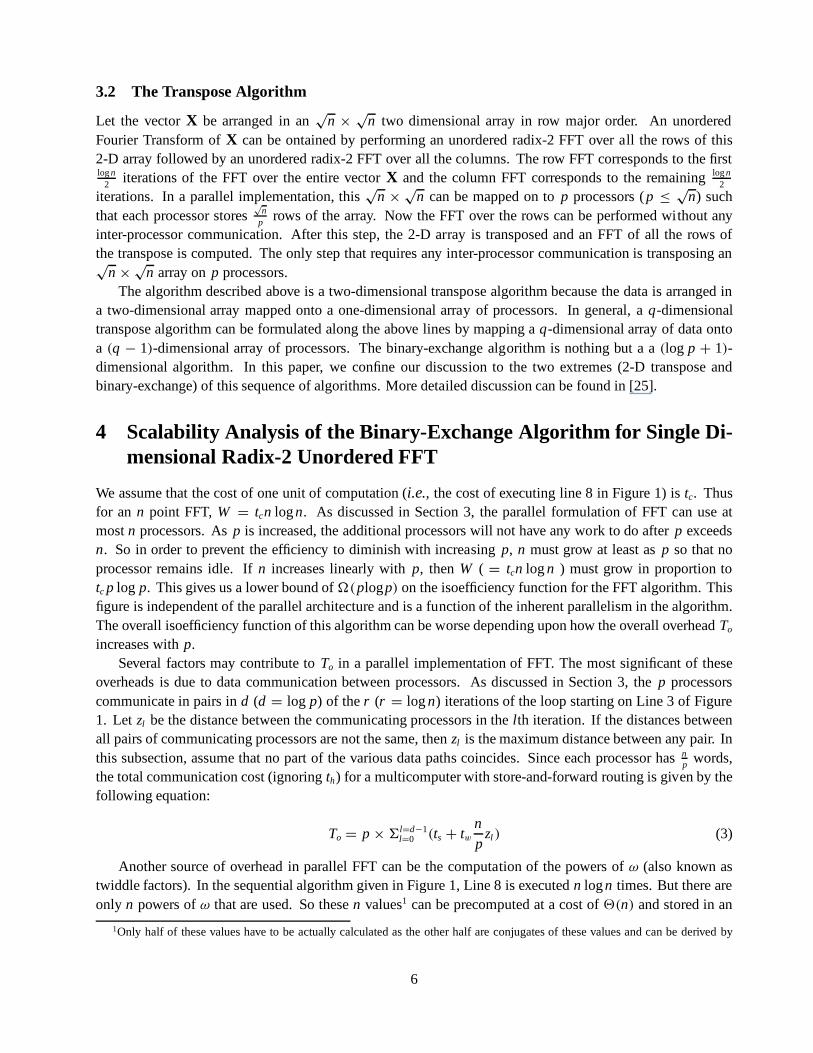
Figure 1 outlines the serial Cooley-Tukey algorithm for an n point single dimensional unordered radix-2 FFTadapted from [2, 36]. X is the input vector of length n (n = 2r for some integer r) and Y is its FourierTransform. ωk denotes the complex number e j 2π

n k, where j =√

−1. More generally, ω is the primitive nth

4

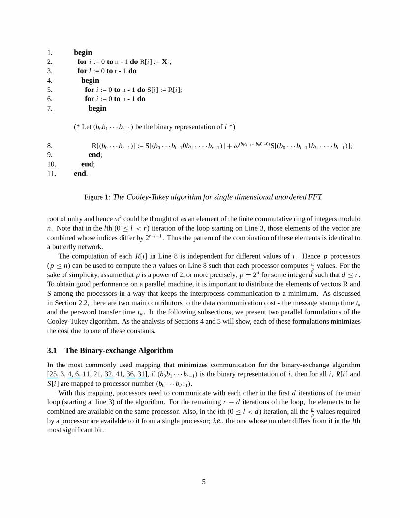
1. begin2. for i := 0 to n - 1 do R[i] := Xi ;3. for l := 0 to r - 1 do4. begin5. for i := 0 to n - 1 do S[i] := R[i];6. for i := 0 to n - 1 do7. begin

(* Let (b0b1 · · ·br−1) be the binary representation of i *)

8. R[(b0 · · ·br−1)] := S[(b0 · · ·bl−10bl+1 · · ·br−1)] + ω(blbl−1···b00···0)S[(b0 · · ·bl−11bl+1 · · ·br−1)];9. end;10. end;11. end.

Figure 1: The Cooley-Tukey algorithm for single dimensional unordered FFT.

root of unity and hence ωk could be thought of as an element of the finite commutative ring of integers modulon. Note that in the lth (0 ≤ l < r) iteration of the loop starting on Line 3, those elements of the vector arecombined whose indices differ by 2r−l−1 . Thus the pattern of the combination of these elements is identical toa butterfly network.

The computation of each R[i] in Line 8 is independent for different values of i. Hence p processors(p ≤ n) can be used to compute the n values on Line 8 such that each processor computes n

pvalues. For the

sake of simplicity, assume that p is a power of 2, or more precisely, p = 2d for some integer d such that d ≤ r .To obtain good performance on a parallel machine, it is important to distribute the elements of vectors R andS among the processors in a way that keeps the interprocess communication to a minimum. As discussedin Section 2.2, there are two main contributors to the data communication cost - the message startup time ts

and the per-word transfer time tw. In the following subsections, we present two parallel formulations of theCooley-Tukey algorithm. As the analysis of Sections 4 and 5 will show, each of these formulations minimizesthe cost due to one of these constants.

3.1 The Binary-exchange Algorithm

In the most commonly used mapping that minimizes communication for the binary-exchange algorithm[25, 3, 4, 6, 11, 21, 32, 41, 36, 31], if (b0b1 · · ·br−1) is the binary representation of i, then for all i, R[i] andS[i] are mapped to processor number (b0 · · ·bd−1).

With this mapping, processors need to communicate with each other in the first d iterations of the mainloop (starting at line 3) of the algorithm. For the remaining r − d iterations of the loop, the elements to becombined are available on the same processor. Also, in the lth (0 ≤ l < d) iteration, all the n

p values requiredby a processor are available to it from a single processor; i.e., the one whose number differs from it in the lthmost significant bit.

5

3.2 The Transpose Algorithm

Let the vector X be arranged in an√

n ×√

n two dimensional array in row major order. An unorderedFourier Transform of X can be ontained by performing an unordered radix-2 FFT over all the rows of this2-D array followed by an unordered radix-2 FFT over all the columns. The row FFT corresponds to the firstlog n

2 iterations of the FFT over the entire vector X and the column FFT corresponds to the remaining log n2

iterations. In a parallel implementation, this√

n ×√

n can be mapped on to p processors ( p ≤√

n) suchthat each processor stores

√n

p rows of the array. Now the FFT over the rows can be performed without anyinter-processor communication. After this step, the 2-D array is transposed and an FFT of all the rows ofthe transpose is computed. The only step that requires any inter-processor communication is transposing an√

n ×√

n array on p processors.The algorithm described above is a two-dimensional transpose algorithm because the data is arranged in

a two-dimensional array mapped onto a one-dimensional array of processors. In general, a q-dimensionaltranspose algorithm can be formulated along the above lines by mapping a q-dimensional array of data ontoa (q − 1)-dimensional array of processors. The binary-exchange algorithm is nothing but a a (log p + 1)-dimensional algorithm. In this paper, we confine our discussion to the two extremes (2-D transpose andbinary-exchange) of this sequence of algorithms. More detailed discussion can be found in [25].

4 Scalability Analysis of the Binary-Exchange Algorithm for Single Di-mensional Radix-2 Unordered FFT

We assume that the cost of one unit of computation (i.e., the cost of executing line 8 in Figure 1) is tc. Thusfor an n point FFT, W = tcn log n. As discussed in Section 3, the parallel formulation of FFT can use atmost n processors. As p is increased, the additional processors will not have any work to do after p exceedsn. So in order to prevent the efficiency to diminish with increasing p, n must grow at least as p so that noprocessor remains idle. If n increases linearly with p, then W ( = tcn log n ) must grow in proportion totc p log p. This gives us a lower bound of �(plogp) on the isoefficiency function for the FFT algorithm. Thisfigure is independent of the parallel architecture and is a function of the inherent parallelism in the algorithm.The overall isoefficiency function of this algorithm can be worse depending upon how the overall overhead To

increases with p.Several factors may contribute to To in a parallel implementation of FFT. The most significant of these

overheads is due to data communication between processors. As discussed in Section 3, the p processorscommunicate in pairs in d (d = log p) of the r (r = log n) iterations of the loop starting on Line 3 of Figure1. Let zl be the distance between the communicating processors in the lth iteration. If the distances betweenall pairs of communicating processors are not the same, then zl is the maximum distance between any pair. Inthis subsection, assume that no part of the various data paths coincides. Since each processor has n

p words,the total communication cost (ignoring th) for a multicomputer with store-and-forward routing is given by thefollowing equation:

To = p × 6l=d−1l=0 (ts + tw

n

pzl ) (3)

Another source of overhead in parallel FFT can be the computation of the powers of ω (also known astwiddle factors). In the sequential algorithm given in Figure 1, Line 8 is executed n log n times. But there areonly n powers of ω that are used. So these n values1 can be precomputed at a cost of 2(n) and stored in an

1Only half of these values have to be actually calculated as the other half are conjugates of these values and can be derived by

6

array before starting the loop at Line 3. As shown in Appendix A, at least some of the processors use a newtwiddle factor in each of the log n iterations. If the FFT of the same size is being computed repeatedly, then thetwiddle factors to be used by each processor can be precomputed and stored. But if that is not the case, thenthe twiddle factor computation is a part of an FFT implementation, and, as shown in Appendix A, an overheadof 2(n + p log p) is incurred due to these extra computations.

4.1 Isoefficiency on a Hypercube

As discussed in Section 3, in the lth iteration of the loop beginning on Line 3 of Figure 1, data messagescontaining n

p words are exchanged between the processors whose binary representations are different in thelth most significant bit position (l < d = log p). Since all these pairs of processors with addresses differingin one bit position are directly connected in a hypercube configuration, Equation (3) becomes:

To = p × 6l=(log p)−1l=0 (ts + tw

n

p)

=> To = ts p log p + twn log p (4)

If p increases, then in order to maintain the efficiency at some value E , W should be equal to K To, whereK = E/(1 − E). Since W = tcn log n, n must grow such that

tcn log n = K (ts p log p + twn log p) (5)

Clearly, the isoefficiency function due to the first term in To, is given by:

W = K ts p log p (6)

The requirement on the growth of W (to maintain a fixed efficiency) due to the second term in To is morecomplicated. If this term requires W to grow at a rate less than 2(p log p), then it can be ignored in favor ofthe first term. On the other hand, if this term requires W to grow at a rate higher than 2(p log p), then the firstterm of To can be ignored.

Balancing W against the second term only yields the following:

ntc log n = K twn log p=> log n = K tw

tclog p

=> n = pK twtc

This leads to the following isoefficiency function (due to the second term of To):

W = K tw × pK twtc × log p (7)

This growth is less than 2(p log p) as long as K twtc

< 1. As soon as this product exceeds 1, the overallisoefficiency function is given by Equation (7). Since the binary-exchange algorithm involves only nearestneighbor communication on a hypercube, the total overhead To, and hence the scalability, cannot be improvedby using cut-through routing.

changing the sign of the imaginary part.

7

4.1.1 Efficiency Threshold

The isoefficiency function given by Equation (7) deteriorates very rapidly with the increase in the value ofK tw

tc. In fact the efficiency corresponding to K tw

tc= 1, (i.e., E = tc

tc+tw) acts somewhat as a threshold value. For

a given hypercube with fixed tc and tw, efficiencies up to this values can be obtained easily. But efficienciesmuch higher than this threshold can be obtained only if the problem size is extremely large. The followingexamples further illustrate the effect of the value of K tw

tcon the isoefficiency function.

Example 1: Consider the computation of an n point FFT on a p-processor hypercube on which tw = tc. Theisoefficiency function of the parallel FFT on this machine is K tw × pK × log p. Now for K < 1 (i.e.E ≤ 0.5) the overall isoefficiency is 2(p log p), but for E > 0.5, the isoefficiency function is muchworse. If E = 0.9, then K = 9 and hence the isoefficiency function becomes 2(p9 log p).

Example 2: Now consider the computation of an n point FFT on a p-processor hypercube on which tw =2tc. Now the threshold efficiency is 0.33. The isoefficiency function for E = 0.5 is 2(p2 log p) and forE = 0.9, it becomes 2(p18 log p).

These examples show how the ratio of tw and tc effects the scalability and how hard it is to obtain efficiencieshigher than the threshold determined by this ratio.

4.2 Isoefficiency on a Mesh

Assume that an n point FFT is being computed on a p-processor simple mesh (√

p rows × √p columns) such

that√

p is a power of 2. For example consider p = 64 such that processor 0,1,2,3,4,5,6,7 form the first row andprocessors 0,8,16,24,32,40,48,56 form the first column. Now during the execution of the algorithm, processor0 will need to communicate with processors 1,2,4,8,16,32. All these communicating processors lie in thesame row or the same column. More precisely, in log

√p of the log p steps that require data communication,

the communicating processors are in the same row, and in the remaining log√

p steps, they are in the samecolumn. The distance between the communicating processors in a row grows from one hop to

√p/2 hops,

doubling in each of the log√

p steps. The communication pattern is similar in case of the columns. The readercan verify that this is true for all the communicating processors in the mesh. Thus, from Equation (3) we get:

To = p × 26l=(log

√p)−1

l=0 (ts + tw np 2l)

=> To = 2p(ts log√

p + tw np (

√p − 1))

To ≈ ts p log p + 2twn√

p (8)

Balancing W against the first term yields the following equation for the isoefficiency function:

W = K ts p log p (9)

Balancing W against the second term yields the following:

tcn log n = 2K tw × n × √p

=> logn = 2K twtc

× √p

=> n = 22K twtc

×√p

8

Since the growth in W required by the third term in To is much higher than that required by the first twoterms (unless p is very small), this is the term that determines the overall isoefficiency function which is givenby the following equation:

W = 2K tw√

p × 22K twtc

√p (10)

From Equation (10), it is obvious that the problem size has to grow exponentially with the number ofprocessors to maintain a constant efficiency; hence the algorithm is not very scalable on a simple mesh. Anydifferent mapping of input vector X on the processors does not reduce the communication overhead. It hasbeen shown [43] that in any mapping, there will be at least one iteration in which the pairs of processors thatneed to communicate will be at least

√p

2hops apart. Hence the expression for To used in the above analysis

cannot be improved by more than a factor of 2.If the mesh is augmented with cut-through routing, the communication term is expected to be smaller than

that for the mesh, but due to the overheads resulting from the contention for communication channels, theoverall To is exactly the same as that given by Equation (8). Hence, as shown in Appendix D, the overallisoefficiency function remains unchanged and the addition of this feature does not offer any performanceimprovement for the FFT algorithm on a mesh.

5 Scalability Analysis of the Transpose Algorithm for Single Dimen-sional Radix-2 Unordered FFT

As discussed earlier in Section 3, the only data communication involved in this algorithm is the transposition ofan

√n ×

√n two dimensional array on p processors. It is easily seen that this involves the communication of

a chunk of unique data of size np2 between every pair of processors. This communication (known as all-to-all

personalized communication) can be performed by executing the following code on each processor:

for i = 1 to p dosend data to processor number (self address ⊕i)

It is shown in [20], that on a hypercube, in each iteration of the above code, each pair of communicatingprocessors have a contention-free communication path. On a hypercube with store-and-forward routing, thiscommunication will take tw

np log p + ts p time. This communication term yields an overhead function which

is identical to the overhead function of the binary exchange algorithm and hence this scheme does not offerany improvement over the binary exchange scheme. However, on a hypercube with cut-through routing, thiscan be done in time tw n

p+ ts p, leading to an overhead function To given by the following equation:

To = twn + ts p2 (11)

The first term of To is independent of p and hence, as p increases, the problem size must increase tobalance the second communication term. For an efficiency E , this yields the following isoefficiency function,where K = E

1−E :

W = K ts p2 (12)

In the transpose algorithm, the mapping of data on the processors requires that√

n ≥ p. Thus, as pincreases, n has to increase as p2, or else some processors will eventually be out of work. This requirementimposes and isoefficiency function of O(p2 log p) due to the limited concurrency of the transpose algorithm.

9

Since the isoefficiency function due to concurrency exceeds the isoefficiency function due to communication,the former (i.e., O(p2 log p)) is also the overall isoefficiency function of the transpose algorithm on a hypercube.

It can be shown that on a mesh architecture, with or without cut-through routing, the transpose algorithmdoes not improve the communication cost over the binary exchange-algorithm.

As mentioned in Section 3, in this paper we have confined our discussion of the transpose algorithm to thetwo-dimensional case. A generalized transpose algorithm and the related performance and scalability analysiscan be found in [25].

5.1 Comparison with Binary-Exchange

As discussed earlier in this paper, an overall isoefficiency function of O(p log p) can be realized by using thebinary exchange algorithm if the efficiency of operation is such that K tw

tc≤ 1. If the desired efficiency is such

that K twtc

= 2, then the overall isoefficiency functions of both the binary-exchange and the transpose schemesare O(p2 log p). When K tw

tc> 2, the transpose algorithm is more scalable than the binary-exchange algorithm

and should be the algorithm of choice provided that n ≥ p2.In the transpose algorithm described in Section 3, the data of size n is arranged in an

√n ×

√n two

dimensional array and is mapped on to a linear array of p processors2 with p =√

nk

, where k is a positiveinteger between 1 and

√n. In a generalization of this method [25, 39], the vector X can be arranged in an

m-dimensional array mapped on to an (m − 1)-dimensional logical array of p processors, where p = nm−1

m

k .The 2-D transpose algorithm discussed in this paper is a special case of this generalization with m = 2 andthe binary-exchange algorithm is a special case for m = (log p + 1). A comparison of Equations (4) and(11) shows that the binary exchange algorithm minimizes the communication overhead due to ts , whereas the2-D transpose algorithm minimizes the overhead due to tw. Also, the binary-exchange algorithm is highlyconcurrent and can use as many as n processors, whereas the concurrency of the 2-D transpose algorithm islimited to

√n processors. By selecting values of m between 2 and (log p+1), it is possible to derive algorithms

whose concurrencies and communication overheads due to ts and tw have intermediate values between thosefor the two algorithms described in this paper [39]. Under certain circumstances, one of these algorithmsmight be the best choice in terms of both concurrency and communication overheads.

6 Impact of Variations of Cooley-Tukey Algorithm on Scalability

Several schemes of computing the DFT have been suggested in literature [34, 45, 37] that involve fewerarithmetic operations on a serial computer than the simple Cooley-Tukey FFT algorithm. Notable among theseare computing the single dimensional FFTs with radix greater than 2 and computing multi-dimensional FFTsby transforming them into a set of one dimensional FFTs using the polynomial transform method. A radix-qFFT is computed by splitting the input sequence of size n into q sequences of size n

q each, computing the qsmaller FFTs and then combining the result. For example, in a radix-4 FFT, each step involves computingfour outputs from four input values and the total number of iterations becomes log4 n instead of log2 n. Theinput length should, of course, be a power of four. It can be shown that despite the reduction in the number ofiterations, the aggregate communication time for a radix-q FFT remains same as that for radix-2. For example,for a radix-4 algorithm on a hypercube, each communication step now involves four processors distributed intwo dimensions rather than two processors in one dimension. On the other hand, the number of multiplicationsin a radix-4 FFT is 25% less than those in a radix-2 FFT [34]. This number can be marginally improvedfurther by going to higher radices. Thus the total useful work is reduced by a constant factor for FFTs with

2It is a logical linear array of processors which are physically connected in a hypercube network.

10

higher radix than 2, but the amount of communication remains the same. Since both To and W remain of thesame order of magnitude, the various isoefficiency functions for a radix-q FFT will be similar to those for theradix-2 FFT with somewhat higher constants.

As described in [34], polynomial transforms can be used to reduce the number of arithmetic operations inmultidimensional FFTs. In particular, the number of multiplications can be reduced by almost 50% on a twodimensional FFT by this method. But the communication overheads in this algorithm are higher and hence,the asymptotic isoefficiency function will not be any better than that for the Cooley-Tukey algorithm.

It will be instructive to see that how much of the gain due to reduction in the number of arithmetic operationscan be carried over to a parallel implementation. Suppose that a parallel algorithm is working at an efficiency E .Now only E ×100% of the total execution time is being spent in performing useful work, while (1− E)×100%time is being spent in communication and other overheads. An r × 100% improvement in the computationalcomplexity of the parent serial algorithm will therefore result in the reduction of the parallel execution timefrom Tp to (1 − E)Tp + (1 − r)ETp - an improvement of Tp−(1−E)Tp−(1−r)ETp

Tp× 100% = r E × 100%. Thus

any improvement in the serial time complexity of an algorithm is dampened by a factor of E in its parallelimplementation if the original parallel algorithm was running at an efficiency E . For example, if the radix-4algorithm reduces the number of arithmetic operations by 25% over the radix-2 algorithm, then on a serialmachine, it will lead to a 33.3% increase in the effective throughput for the FFT computation; i.e., by improvingthe algorithm, an M Mega-FLOPS machine will deliver performance equivalent to that of a 1.33M Mega-FLOPS machine running the unimproved algorithm. On the other hand, a similar improvement will result ina throughput increase of only 14% for a parallel machine with the same aggregate computing power workingat 50% efficiency.

As discussed in Section 4.1.1, for the binary-exchange algorithm it is hard to achieve efficiencies muchhigher than the threshold given by tc

tc+twon a hypercube. But if the threshold is much above 0.5, then substantial

performance improvements can be obtained by improving the parent serial algorithm. If the threshold is muchbelow 0.5, it is better to concentrate on reducing the communication rather than computation cost to attainhigher performance.

7 Cost-Effectiveness of Mesh and Hypercube for FFT Computation

The scalability of a certain algorithm-architecture combination determines its capability to use increasingnumber of processors effectively. Many algorithms may be more scalable on costlier architectures. In suchsituations, one needs to consider whether it is better to have a larger parallel computer of a cost-wise morescalable architecture that is underutilized (because of poor efficiency), or to have a smaller parallel computerof a cost-wise less scalable architecture that is better utilized. For a given amount of resources, the aim isto maximize the overall performance which is proportional to the number of processors and the efficiencyobtained on them. From the scalability analysis of Section 4, it can be predicted that the FFT algorithmwill perform much poorly on a mesh as compared to a hypercube. On the other hand constructing a meshmulticomputer is cheaper than constructing a hypercube with the same number of processors. In this sectionwe show that in spite of this, it might be more cost-effective to implement FFT on a hypercube rather than ona mesh.

Suppose that the cost of building a communication network for a parallel computer is directly proportionalto the number of communication links. If we neglect the effect of the length of the links (i.e., th = 0) andassume that ts = 0, then the efficiency of an n point FFT computation using the binary-exchange scheme isapproximately given by (1 + tw log p

tc log n )−1 on a p processor hypercube and by (1 + 2tw√

ptc log n )−1 on a p processor

mesh. It is assumed here that tw and tc are same for both the computers. Now it is possible to obtain similar

11

performance on both the computers if we make each channel on the mesh w wide (thus effectively reducingthe per-word communication time to tw

w), choosing w such that 2

√p

w= log p. The cost of constructing these

hypercube and mesh networks will be p log p and 4wp respectively, where w = 2√

plog p . Since 8p

√p

log p is greater

than p log p for all p (it is easier to see that 8√

p(log p)2 > 1 for all p), it will be cheaper to obtain the same

performance for FFT computation on a hypercube than on a mesh. If the comparison is based on the transposealgorithm, then the hypercube will turn out to be even more cost effective, as the factor w by which thebandwidth of the mesh channels will have to be increased to match its performance with that of a hypercubewill now be

√p. Thus the relative costs of building a mesh and a hypercube with identical performance for

the FFT computation will be 8p√

p and p log p, respectively.However, if the cost of the network is considered to be a function of the bisection width of the network, as

may be the case in VLSI implementations [10], then the picture improves for the mesh. The bisection widthsof a hypercube and a mesh containing p processors each are p

2 and√

p respectively. In order to match theperformance of the mesh with that of the hypercube for the binary-exchange algorithm, each of its channelshas to made wider by a factor of w = 2

√p

log p. In this case, the bisection width of the mesh network becomes

2 plog p . Thus the costs of the hypercube and mesh networks with p processors each, such that they yield similar

performance on the FFT, will be functions of p2 and 2 p

log p , respectively. Clearly, for p > 256, such a meshnetwork is cheaper to build than a hypercube. However, for the transpose algorithm the relative costs of themesh and the hypercube yielding same throughput will be p

2and 2p, respectively. Hence the hypercube is still

more cost effective by a constant factor.The above analysis shows that the performance of the FFT algorithm on a mesh can be improved con-

siderably by increasing the bandwidth of its communication channels by a factor of√

p

2. But the enhanced

bandwidth can be fully utilized only if there are at least√

p4 data items to be transferred in each communication

step. Thus the input data size n should be at least p√

p4 . This leads to an isoefficiency term of O(p1.5 log p) due

to concurrency, but is still a significant improvement for the mesh from O(√

p22K twtc ) with channels of constant

bandwidth. In fact O(p1.5 log p) is the best possible isoefficiency for FFT on a mesh even if the channel widthis increased arbitrarily with the number of processors. It can be shown that if the channel bandwidth grows asO(px), then the isoefficiency function due to communication will be O(p.5−x22K tw

tcp.5−x

) and the isoefficiencyfunction due to concurrency will be O(p1+x log p). If x < 0.5, then the overall isoefficiency is determinedby communication overheads, and is exponential. If x ≥ 0.5, then the overall isoefficiency is determined byconcurrency. Thus, the best isoefficiency function of O(p1.5 log p) can be obtained at x = .5.

8 Experimental Results

We implemented the binary-exchange algorithm for unordered single dimensional radix-2 FFT on a 1024-nodenCUBE1 hypercube. Experiments were conducted for a range of problem sizes and a range of machine sizes;i.e., number of processors. The length of the input vector was varied between 4 and 65536, and the numberof processors was varied between 1 and 1024. The required twiddle factors were precomputed and stored ateach processor. Speedups and efficiencies were computed w.r.t. the run time of sequential FFT running onone processor of the nCUBE1. A unit FFT computation takes3 approximately 80 microseconds; i.e., tc ≈ 80

3In our actual FFT program written in C a unit of computation took approximately 400 microseconds. Given that each FFTcomputation requires four 32-bit additions/subtractions and four 32 bit multiplications, this corresponds to a Mega-FLOP rating of0.02 which is far lower than those obtained from FFT benchmarks written in Fortran or assembly language. This is perhaps due to ourinefficient C-compiler. Since CPU speed has a tremendous impact on the overall scalability of FFT, we artificially increased the CPUspeed to a more realistic rating of 0.1 Mega-FLOP. This is obtained by replacing the actual complex arithmetic of the inner loop of theFFT computation by a dummy loop that takes 80 microseconds to execute.

12

0

100

200

300

400

500

600

700

800

900

0 200 400 600 800 1000

↑S

p →

n = 1024 3333 3 3 3 3n = 8192 +

++++

+

+

+

n = 65536 2222 2 2 2 2Linear

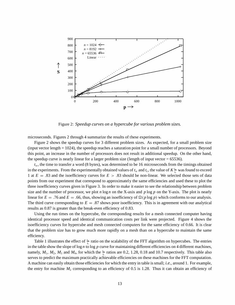
Figure 2: Speedup curves on a hypercube for various problem sizes.

microseconds. Figures 2 through 4 summarize the results of these experiments.Figure 2 shows the speedup curves for 3 different problem sizes. As expected, for a small problem size

(input vector length = 1024), the speedup reaches a saturation point for a small number of processors. Beyondthis point, an increase in the number of processors does not result in additional speedup. On the other hand,the speedup curve is nearly linear for a larger problem size (length of input vector = 65536).

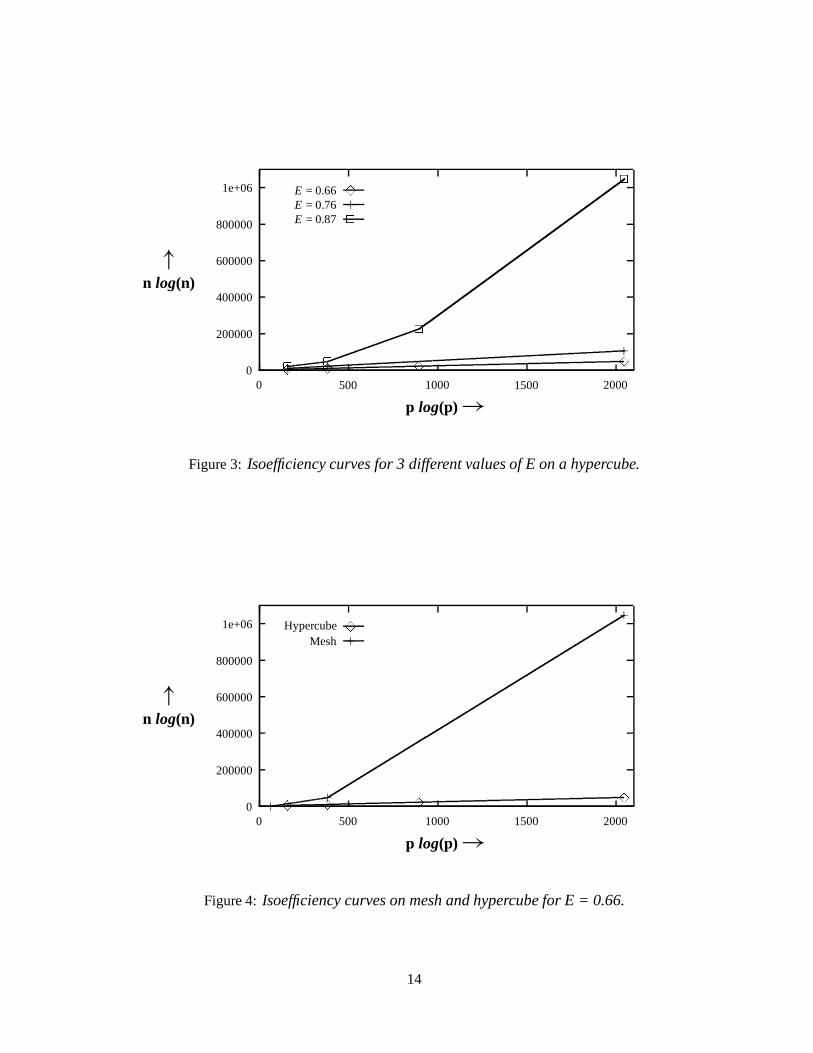
tw, the time to transfer a word (8 bytes), was determined to be 16 microseconds from the timings obtainedin the experiments. From the experimentally obtained values of tw and tc, the value of K tw

tcwas found to exceed

1 at E = .83 and the isoefficiency curves for E > .83 should be non-linear. We selected those sets of datapoints from our experiment that correspond to approximately the same efficiencies and used these to plot thethree isoefficiency curves given in Figure 3. In order to make it easier to see the relationship between problemsize and the number of processor, we plot n log n on the X-axis and p log p on the Y-axis. The plot is nearlylinear for E = .76 and E = .66, thus, showing an isoefficiency of �(p log p) which conforms to our analysis.The third curve corresponding to E = .87 shows poor isoefficiency. This is in agreement with our analyticalresults as 0.87 is greater than the break-even efficiency of 0.83.

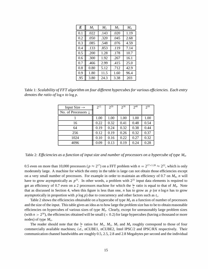
Using the run times on the hypercube, the corresponding results for a mesh connected computer havingidentical processor speed and identical communication costs per link were projected. Figure 4 shows theisoefficiency curves for hypercube and mesh connected computers for the same efficiency of 0.66. It is clearthat the problem size has to grow much more rapidly on a mesh than on a hypercube to maintain the sameefficiency.

Table 1 illustrates the effect of twtc

ratio on the scalability of the FFT algorithm on hypercubes. The entriesin the table show the slope of log n to log p curve for maintaining different efficiencies on 4 different machines,namely, M1, M2, M3 and M4, for which the tw

tcratios are 0.2, 1.28, 0.18 and 10.7 respectively. This table also

serves to predict the maximum practically achievable efficiencies on these machines for the FFT computation.A machine can easily obtain those efficiencies for which the entry in table is small; i.e., around 1. For example,the entry for machine M2 corresponding to an efficiency of 0.5 is 1.28. Thus it can obtain an efficiency of

13

0

200000

400000

600000

800000

1e+06

0 500 1000 1500 2000

↑n log(n)

p log(p) →

E = 0.66 33 3 3 3E = 0.76 +

+ ++

E = 0.87 22 2 2 2Figure 3: Isoefficiency curves for 3 different values of E on a hypercube.

0

200000

400000

600000

800000

1e+06

0 500 1000 1500 2000

↑n log(n)

p log(p) →

Hypercube 33 3 3 3Mesh +

++

+

Figure 4: Isoefficiency curves on mesh and hypercube for E = 0.66.

14

E M1 M2 M3 M4

0.1 .022 .143 .020 1.190.2 .050 .320 .045 2.680.3 .085 .548 .076 4.590.4 .133 .853 .119 7.140.5 .200 1.28 .178 10.70.6 .300 1.92 .267 16.10.7 .466 2.99 .415 25.00.8 0.80 5.12 .712 42.90.9 1.80 11.5 1.60 96.4.95 3.80 24.3 3.38 203

Table 1: Scalability of FFT algorithm on four different hypercubes for various efficiencies. Each entrydenotes the ratio of log n to log p.

Input Size → 212 220 230 240 250

No. of Processors ↓1 1.00 1.00 1.00 1.00 1.0016 0.22 0.32 0.41 0.48 0.5464 0.19 0.24 0.32 0.38 0.44256 0.12 0.19 0.26 0.32 0.37

1024 0.10 0.16 0.22 0.27 0.324096 0.09 0.13 0.19 0.24 0.28

Table 2: Efficiencies as a function of input size and number of processors on a hypercube of type M4.

0.5 even on more than 10,000 processors ( p ≈ 217) on a FFT problem with n = 217×1.28 ≈ 222, which is onlymoderately large. A machine for which the entry in the table is large can not obtain those efficiencies excepton a very small number of processors. For example in order to maintain an efficiency of 0.7 on M4, n willhave to grow asymptotically as p25. In other words, a problem with 225 input data elements is required toget an efficiency of 0.7 even on a 2 processors machine for which the tw

tcratio is equal to that of M4. Note

that as discussed in Section 4, when this figure is less than one, n has to grow as p (or n log n has to growasymptotically in proportion with p log p) due to concurrency and other factors such as ts .

Table 2 shows the efficiencies obtainable on a hypercube of type M4 as a function of number of processorsand the size of the input. This table gives an idea as to how large the problem size has to be to obtain reasonableefficiencies on hypercubes of various sizes of type M4. Clearly, except for unreasonably large problem sizes(with n > 230), the efficiencies obtained will be small (< 0.2) for large hypercubes (having a thousand or morenodes) of type M4.

The reader should note that the twtc

ratios for M1, M2, M3 and M4 roughly correspond to those of fourcommercially available machines; i.e., nCUBE1, nCUBE2, Intel IPSC/2 and IPSC/RX respectively. Theircommunication channel bandwidths are roughly 0.5, 2.5, 2.8 and 2.8 Megabytes per second and the individual

15

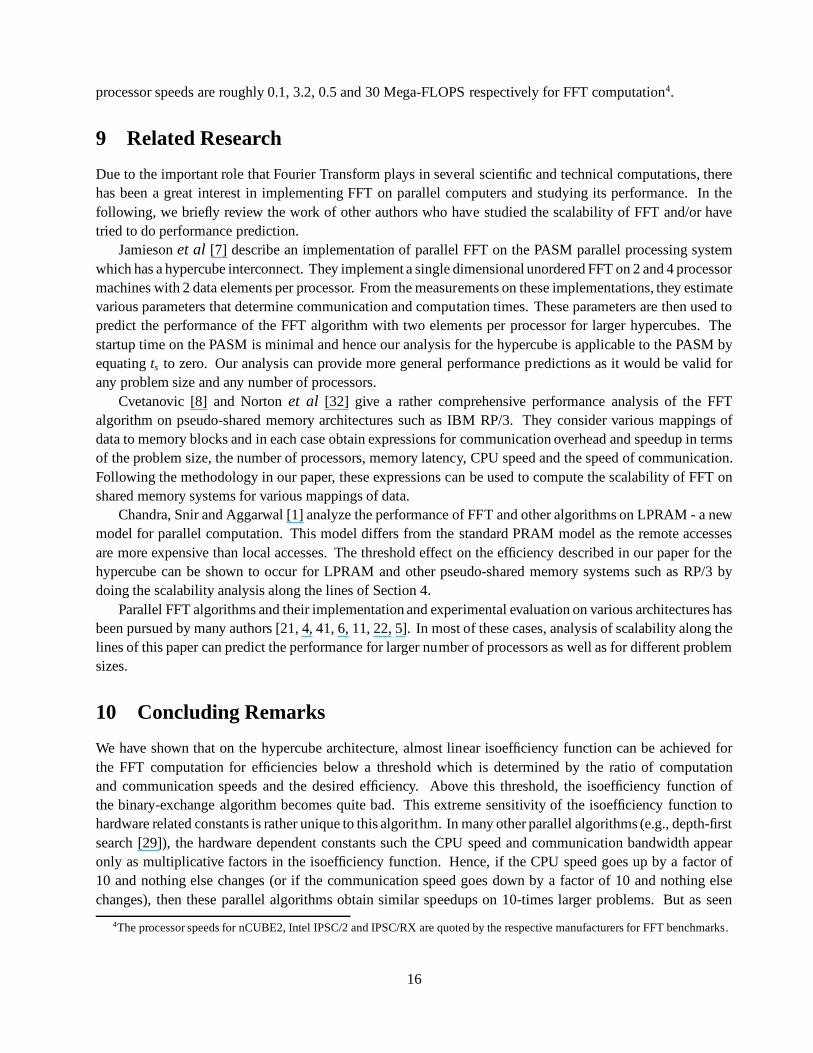
processor speeds are roughly 0.1, 3.2, 0.5 and 30 Mega-FLOPS respectively for FFT computation4.

9 Related Research

Due to the important role that Fourier Transform plays in several scientific and technical computations, therehas been a great interest in implementing FFT on parallel computers and studying its performance. In thefollowing, we briefly review the work of other authors who have studied the scalability of FFT and/or havetried to do performance prediction.

Jamieson et al [7] describe an implementation of parallel FFT on the PASM parallel processing systemwhich has a hypercube interconnect. They implement a single dimensional unordered FFT on 2 and 4 processormachines with 2 data elements per processor. From the measurements on these implementations, they estimatevarious parameters that determine communication and computation times. These parameters are then used topredict the performance of the FFT algorithm with two elements per processor for larger hypercubes. Thestartup time on the PASM is minimal and hence our analysis for the hypercube is applicable to the PASM byequating ts to zero. Our analysis can provide more general performance predictions as it would be valid forany problem size and any number of processors.

Cvetanovic [8] and Norton et al [32] give a rather comprehensive performance analysis of the FFTalgorithm on pseudo-shared memory architectures such as IBM RP/3. They consider various mappings ofdata to memory blocks and in each case obtain expressions for communication overhead and speedup in termsof the problem size, the number of processors, memory latency, CPU speed and the speed of communication.Following the methodology in our paper, these expressions can be used to compute the scalability of FFT onshared memory systems for various mappings of data.

Chandra, Snir and Aggarwal [1] analyze the performance of FFT and other algorithms on LPRAM - a newmodel for parallel computation. This model differs from the standard PRAM model as the remote accessesare more expensive than local accesses. The threshold effect on the efficiency described in our paper for thehypercube can be shown to occur for LPRAM and other pseudo-shared memory systems such as RP/3 bydoing the scalability analysis along the lines of Section 4.

Parallel FFT algorithms and their implementation and experimental evaluation on various architectures hasbeen pursued by many authors [21, 4, 41, 6, 11, 22, 5]. In most of these cases, analysis of scalability along thelines of this paper can predict the performance for larger number of processors as well as for different problemsizes.

10 Concluding Remarks

We have shown that on the hypercube architecture, almost linear isoefficiency function can be achieved forthe FFT computation for efficiencies below a threshold which is determined by the ratio of computationand communication speeds and the desired efficiency. Above this threshold, the isoefficiency function ofthe binary-exchange algorithm becomes quite bad. This extreme sensitivity of the isoefficiency function tohardware related constants is rather unique to this algorithm. In many other parallel algorithms (e.g., depth-firstsearch [29]), the hardware dependent constants such the CPU speed and communication bandwidth appearonly as multiplicative factors in the isoefficiency function. Hence, if the CPU speed goes up by a factor of10 and nothing else changes (or if the communication speed goes down by a factor of 10 and nothing elsechanges), then these parallel algorithms obtain similar speedups on 10-times larger problems. But as seen

4The processor speeds for nCUBE2, Intel IPSC/2 and IPSC/RX are quoted by the respective manufacturers for FFT benchmarks.

16

in Example 2 and Table 2, for parallel FFT, even a factor of 2 change in the ratio of computation speed tocommunication speed causes the scalability to change quite drastically. Similarly, an improvement in theserial algorithm that reduces only the amount of computation will result in a much smaller improvement in theexecution time of the parallel implementation of the algorithm. These effects are more pronounced for a largenumber of processors.

If the hypercube supports cut-through routing, then it is possible to overcome this thresholding effect byusing the transpose algorithm. The overall scalability of the transpose algorithm is O(p2), but it stays stablefor much higher efficiencies than in case of the binary-exchange algorithm. The choice between the twoalgorithms depends upon the communication related parameters (i.e., ts and tw) of the machine in use, the sizeof the problem to be solved and the number of processors available.

The isoefficiency function of parallel FFT on the 2-D mesh architecture is exponential; hence the speedupand efficiency on large-scale mesh connected multicomputers will be poor except on unreasonably largeproblem instances. It is often claimed that adding worm-hole routing feature to multicomputers makes themas powerful as fully connected multicomputers. This is indeed the case if the message start-up time, ts , is largeand if the sharing of data paths among the messages traveling simultaneously is not significant. But for theFFT computation on meshes, it does not offer any improvement in the overall scalability. The scalability ofFFT on a mesh can be improved considerably if the width of inter-processor links is increased as a function ofthe number of processors p. The optimal isoefficiency function for the mesh is O(p1.5 log p) and is achievedwhen the bandwidth of the communication channels is increased as O(

√p). The reader can verify that the

isoefficiency function of FFT on 3-D mesh architecture is also exponential and can be derived by an analysissimilar to the one given for the 2-D mesh in this paper.

Analysis very similar to that in Section 4 can be performed to obtain the isoefficiency functions for the FFTalgorithm on other types of architectures. For example, the isoefficiency analysis for a MIMD hypercube/meshin Section 4 is directly applicable to a SIMD hypercube/mesh if the message startup time is ignored. Similarly,if ts and th are considered zero and tw is considered to be the latency due to non-local memory access, theanalysis for the hypercube is applicable for a shared memory architecture because on the hypercube, eachcommunication occurs between directly connected processors.

Different parallel architectures such as mesh, hypercube, and omega-network-based shared memory ar-chitectures have different scalability from the viewpoint of cost. Our analysis in Section 7 shows that for theFFT computation, hypercube is more cost-effective than a 2-D mesh even if the cost of the communicationnetwork based on the total number of communication channels is taken into account. Similar conclusions canbe drawn for a 3-D mesh as well.

Acknowledgement

The authors wish to thank John Gustafson, David Bailey and Nageshwara Rao Vempaty for making a numberof useful suggestions on an earlier draft of this paper. The authors also thank Sandia National Labs forproviding access to their 1024-processor nCUBE1.

References[1] Alok Aggarwal, Ashok K. Chandra, and Mark Snir. Communication complexity of PRAMs. Technical Report RC 14998 (No.

64644), IBM T. J. Watson Research Center, Yorktown Heights, NY, Yorktown Heights, NY, 1989.

[2] A. V. Aho, John E. Hopcroft, and J. D. Ullman. The Design and Analysis of Computer Algorithms. Addison-Wesley, Reading,MA, 1974.

[3] S. G. Akl. The Design and Analysis of Parallel Algorithms. Prentice-Hall, Englewood Cliffs, NJ, 1989.

17

[4] A. Averbuch, E. Gabber, B. Gordissky, and Y. Medan. A parallel FFT on an MIMD machine. Parallel Computing, 15:61–74,1990.

[5] David H. Bailey. FFTs in external or hierarchical memory. The Journal of Supercomputing, 4:23–35, 1990.

[6] S. Bershader, T. Kraay, and J. Holland. The giant-Fourier-transform. In Proceedings of the Fourth Conference on Hypercubes,Concurrent Computers, and Applications: Volume I, pages 387–389, 1989.

[7] Edward C. Bronson, Thomas L. Casavant, and L. H. Jamieson. Experimental application-driven architecture analysis of anSIMD/MIMD parallel processing system. IEEE Transactions on Parallel and Distributed Systems, 1(2):195–205, 1990.

[8] Z. Cvetanovic. Performance analysis of the FFT algorithm on a shared-memory parallel architecture. IBM Journal of Researchand Development, 31(4):435–451, 1987.

[9] William J. Dally. A VLSI Architecture for Concurrent Data Structures. Kluwer Academic Publishers, Boston, MA, 1987.

[10] William J. Dally. Wire-efficienct VLSI multiprocessor communication network. In Stanford Conference on Advanced Researchin VLSI Networks, pages 391–415, 1987.

[11] Laurent Desbat and Denis Trystram. Implementing the discrete Fourier transform on a hypercube vector-parallel computer. InProceedings of the Fourth Conference on Hypercubes, Concurrent Computers, and Applications: Volume I, pages 407–410,1989.

[12] D. L. Eager, J. Zahorjan, and E. D. Lazowska. Speedup versus efficiency in parallel systems. IEEE Transactions on Computers,38(3):408–423, 1989.

[13] Ananth Grama, Anshul Gupta, and Vipin Kumar. Isoefficiency: Measuring the scalability of parallel algorithms and architectures.IEEE Parallel and Distributed Technology, 1(3):12–21, August, 1993. Also available as Technical Report TR 93-24, Departmentof Computer Science, University of Minnesota, Minneapolis, MN.

[14] Anshul Gupta and Vipin Kumar. On the scalability of FFT on parallel computers. In Proceedings of the Third Symposium onthe Frontiers of Massively Parallel Computation, 1990. Also available as Technical Report TR 90-53, Department of ComputerScience, University of Minnesota, Minneapolis, MN.

[15] Anshul Gupta and Vipin Kumar. The scalability of matrix multiplication algorithms on parallel computers. Technical ReportTR 91-54, Department of Computer Science, University of Minnesota, Minneapolis, MN, 1991. A short version appears inProceedings of 1993 International Conference on Parallel Processing, pages III-115–III-119, 1993.

[16] Anshul Gupta, Vipin Kumar, and A. H. Sameh. Performance and scalability of preconditioned conjugate gradient methods onparallel computers. Technical Report TR 92-64, Department of Computer Science, University of Minnesota, Minneapolis, MN,1992. A short version appears in Proceedings of the Sixth SIAM Conference on Parallel Processing for Scientific Computing,pages 664–674, 1993.

[17] John L. Gustafson. Reevaluating Amdahl’s law. Communications of the ACM, 31(5):532–533, 1988.

[18] John L. Gustafson, Gary R. Montry, and Robert E. Benner. Development of parallel methods for a 1024-processor hypercube.SIAM Journal on Scientific and Statistical Computing, 9(4):609–638, 1988.

[19] Kai Hwang. Advanced Computer Architecture: Parallelism, Scalability, Programmability. McGraw-Hill, New York, NY, 1993.

[20] S. L. Johnsson and C.-T. Ho. Optimum broadcasting and personalized communication in hypercubes. IEEE Transactions onComputers, 38(9):1249–1268, September 1989.

[21] S. L. Johnsson, R. Krawitz, R. Frye, and D. McDonald. A radix-2 FFT on the connection machine. Technical report, ThinkingMachines Corporation, Cambridge, MA, 1989.

[22] Ray A. Kamin and George B. Adams. Fast Fourier transform algorithm design and tradeoffs. Technical Report RIACS TR 88.18,NASA Ames Research Center, Moffet Field, CA, 1988.

[23] Alan H. Karp and Horace P. Flatt. Measuring parallel processor performance. Communications of the ACM, 33(5):539–543,1990.

[24] Kouichi Kimura and Ichiyoshi Nobuyuki. Probabilistic analysis of the efficiency of the dynamic load distribution. In The SixthDistributed Memory Computing Conference Proceedings, 1991.

[25] Vipin Kumar, Ananth Grama, Anshul Gupta, and George Karypis. Introduction to Parallel Computing: Design and Analysis ofAlgorithms. Benjamin/Cummings, Redwood City, CA, 1994.

[26] Vipin Kumar and Anshul Gupta. Analyzing scalability of parallel algorithms and architectures. Technical Report TR 91-18,Department of Computer Science Department, University of Minnesota, Minneapolis, MN, 1991. To appear in Journal ofParallel and Distributed Computing, 1994. A shorter version appears in Proceedings of the 1991 International Conference onSupercomputing, pages 396-405, 1991.

18

[27] Vipin Kumar and V. N. Rao. Parallel depth-first search, part II: Analysis. International Journal of Parallel Programming,16(6):501–519, 1987.

[28] Vipin Kumar and V. N. Rao. Load balancing on the hypercube architecture. In Proceedings of the Fourth Conference onHypercubes, Concurrent Computers, and Applications, pages 603–608, 1989.

[29] Vipin Kumar and V. N. Rao. Scalable parallel formulations of depth-first search. In Vipin Kumar, P. S. Gopalakrishnan, andLaveen N. Kanal, editors, Parallel Algorithms for Machine Intelligence and Vision. Springer-Verlag, New York, NY, 1990.

[30] Vipin Kumar and Vineet Singh. Scalability of parallel algorithms for the all-pairs shortest path problem. Journal of Paralleland Distributed Computing, 13(2):124–138, October 1991. A short version appears in the Proceedings of the InternationalConference on Parallel Processing, 1990.

[31] Charles Van Loan. Computational Frameworks for the Fast Fourier Transform. SIAM, Philadelphia, PA, 1992.

[32] A. Norton and A. J. Silberger. Parallelization and performance analysis of the Cooley-Tukey FFT algorithm for shared memoryarchitectures. IEEE Transactions on Computers, C-36(5):581–591, 1987.

[33] Daniel Nussbaum and Anant Agarwal. Scalability of parallel machines. Communications of the ACM, 34(3):57–61, 1991.

[34] H. J. Nussbaumer. Fast Fourier Transform and Convolution Algorithms. Springer-Verlag, New York, NY, 1982.

[35] M. C. Pease. The indirect binary n-cube microprocessor array. IEEE Transactions on Computers, 26:458–473, 1977.

[36] Michael J. Quinn. Designing Efficient Algorithms for Parallel Computers. McGraw-Hill, New York, NY, 1987.

[37] C. M. Rader and N. M. Brenner. A new principle for Fast fourier transform. IEEE Transactions on Acoustics, Speech and SignalProcessing, 24:264–265, 1976.

[38] S. Ranka and S. Sahni. Hypercube Algorithms for Image Processing and Pattern Recognition. Springer-Verlag, New York, NY,1990.

[39] V. N. Rao. Personal Communication. University of Central Florida, Orlando, FL, 1992.

[40] Vineet Singh, Vipin Kumar, Gul Agha, and Chris Tomlinson. Scalability of parallel sorting on mesh multicomputers. InternationalJournal of Parallel Programming, 20(2), 1991.

[41] P. N. Swarztrauber. Multiprocessor FFTs. Parallel Computing, 5:197–210, 1987.

[42] Zhimin Tang and Guo-Jie Li. Optimal granularity of grid iteration problems. In Proceedingsof the 1990 International Conferenceon Parallel Processing, pages I111–I118, 1990.

[43] Clark D. Thompson. Fourier transforms in VLSI. IBM Journal of Research and Development, C-32(11):1047–1057, 1983.

[44] Fredric A. Van-Catledge. Towards a general model for evaluating the relative performance of computer systems. InternationalJournal of Supercomputer Applications, 3(2):100–108, 1989.

[45] S. Winograd. A new method for computing DFT. In IEEE International Conferenceon Acoustics, Speech and Signal Processing,pages 366–368, 1977.

[46] Jinwoon Woo and Sartaj Sahni. Hypercube computing: Connectedcomponents. Journalof Supercomputing, 1991. Also availableas TR 88-50 from the Department of Computer Science, University of Minnesota, Minneapolis, MN.

[47] Jinwoon Woo and Sartaj Sahni. Computing biconnected components on a hypercube. Journal of Supercomputing, June 1991.Also available as Technical Report TR 89-7 from the Department of Computer Science, University of Minnesota, Minneapolis,MN.

[48] Patrick H. Worley. The effect of time constraints on scaled speedup. SIAM Journal on Scientific and Statistical Computing,11(5):838–858, 1990.

[49] J. R. Zorbas, D. J. Reble, and R. E. VanKooten. Measuring the scalability of parallel computer systems. In Supercomputing ’89Proceedings, pages 832–841, 1989.

19

i→ 0 1 2 3 4 5 6 7l↓0 000 000 000 000 100 100 100 1001 000 000 100 100 010 010 110 1102 000 100 010 110 001 101 011 111

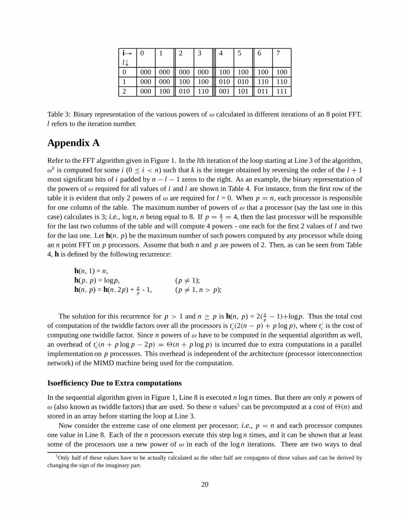
Table 3: Binary representation of the various powers of ω calculated in different iterations of an 8 point FFT.l refers to the iteration number.

Appendix A

Refer to the FFT algorithm given in Figure 1. In the lth iteration of the loop starting at Line 3 of the algorithm,ωk is computed for some i (0 ≤ i < n) such that k is the integer obtained by reversing the order of the l + 1most significant bits of i padded by n − l − 1 zeros to the right. As an example, the binary representation ofthe powers of ω required for all values of i and l are shown in Table 4. For instance, from the first row of thetable it is evident that only 2 powers of ω are required for l = 0. When p = n, each processor is responsiblefor one column of the table. The maximum number of powers of ω that a processor (say the last one in thiscase) calculates is 3; i.e., log n, n being equal to 8. If p = n

2 = 4, then the last processor will be responsiblefor the last two columns of the table and will compute 4 powers - one each for the first 2 values of l and twofor the last one. Let h(n, p) be the maximum number of such powers computed by any processor while doingan n point FFT on p processors. Assume that both n and p are powers of 2. Then, as can be seen from Table4, h is defined by the following recurrence:

h(n, 1) = n,h(p, p) = logp, (p 6= 1);h(n, p) = h(n, 2p) + n

p - 1, (p 6= 1, n > p);

The solution for this recurrence for p > 1 and n ≥ p is h(n, p) = 2( np − 1)+logp. Thus the total cost

of computation of the twiddle factors over all the processors is t ′c(2(n − p) + p log p), where t ′

c is the cost ofcomputing one twiddle factor. Since n powers of ω have to be computed in the sequential algorithm as well,an overhead of t ′

c(n + p log p − 2p) = 2(n + p log p) is incurred due to extra computations in a parallelimplementation on p processors. This overhead is independent of the architecture (processor interconnectionnetwork) of the MIMD machine being used for the computation.

Isoefficiency Due to Extra computations

In the sequential algorithm given in Figure 1, Line 8 is executed n log n times. But there are only n powers ofω (also known as twiddle factors) that are used. So these n values5 can be precomputed at a cost of 2(n) andstored in an array before starting the loop at Line 3.

Now consider the extreme case of one element per processor; i.e., p = n and each processor computesone value in Line 8. Each of the n processors execute this step log n times, and it can be shown that at leastsome of the processors use a new power of ω in each of the log n iterations. There are two ways to deal

5Only half of these values have to be actually calculated as the other half are conjugates of these values and can be derived bychanging the sign of the imaginary part.

20

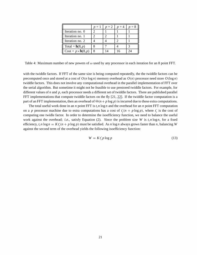
p = 1 p = 2 p = 4 p = 8Iteration no. 0 2 1 1 1Iteration no. 1 2 2 1 1Iteration no. 2 4 4 2 1

Total = h(8,p) 8 7 4 3Cost = p×h(8,p) 8 14 16 24

Table 4: Maximum number of new powers of ω used by any processor in each iteration for an 8 point FFT.

with the twiddle factors. If FFT of the same size is being computed repeatedly, the the twiddle factors can beprecomputed once and stored at a cost of O(n log n) memory overhead as O(n) processor need store O(log n)

twiddle factors. This does not involve any computational overhead in the parallel implementation of FFT overthe serial algorithm. But sometime it might not be feasible to use prestored twiddle factors. For example, fordifferent values of n and p, each processor needs a different set of twiddle factors. There are published parallelFFT implementations that compute twiddle factors on the fly [21, 22]. If the twiddle factor computation is apart of an FFT implementation, then an overhead of 2(n+ p log p) is incurred due to these extra computations.

The total useful work done in an n point FFT is tcn log n and the overhead for an n point FFT computationon a p processor machine due to extra computations has a cost of t ′

c(n + p log p), where t ′c is the cost of

computing one twidle factor. In order to determine the isoefficiency function, we need to balance the usefulwork against the overhead; i.e., satisfy Equation (2). Since the problem size W is tcn log n, for a fixedefficiency, tcn log n = K t ′

c(n + p log p) must be satisfied. As n log n always grows faster than n, balancing Wagainst the second term of the overhead yields the following isoefficiency function:

W = K t ′c p log p (13)

21

Appendix B

Some Other Scalability Metrics

Apart from the isoefficiency function, some other metrics have been proposed to study the scalability of parallelalgorithm architecture combinations. Here we present a brief6 scalability analysis of the 1-D unordered radix-2FFT using these metrics.

Gustafson, Montry and Benner [18, 17] were the first to experimentally demonstrate that by scaling up theproblem size one can obtain near-linear speedup on as many as 1024 processors. Gustafson et. al. introduceda new metric called “scaled speedup” to evaluate the performance on practically feasible architectures. Thismetric is defined as the speedup curve obtained when the problem size is increased linearly with the numberof processors. If the scaled-speedup curve is good (e.g., close to linear), then the algorithm-architecturecombination is considered scalable. The scaled speedup for the FFT when the problem size grows linearlywith p (i.e., tcn log n = p) is approximately tc p

tc+twon a hypercube and tc p

tc+tw√

plog p

on a mesh within double log

terms. It is clear that the algorithm attains near linear speedup on the hypercube, whereas the speedup on themesh is much worse.

Karp and Flatt [23] introduced experimentally determined serial fraction f as a new metric for measuringthe performance of a parallel system on a fix-sized problem. If S is the speedup on a p-processor system,then f is defined as 1/S−1/p

1−1/p . Smaller values of f are considered better. If f increases with the number ofprocessors, then it is considered as an indicator of rising communication overhead, and thus an indicator ofpoor scalability. The values of Karp and Flatt’s serial fraction are tw log p

tc p log n and twtc√

p log n for the hypercube and themesh respectively. Clearly the serial fraction is much lower on a hypercube than on a mesh.

Zorbas et. al. [49] introduce the concept of an overhead function 8(p). A p-processor system scales withoverhead 8(p) if the run time TP on p processors satisfies TP ≤ C(Ws + Wp

p ) × 8(p). The smallest overhead

function that satisfies this equation is called the systems overhead function and is defined by TP

C(Ws +Wp/p). The

values of Zorbas’ overhead function for the two architectures are 1 + tw log ptc log n (hypercube) and 1 + tw

√p

tc log n (mesh)respectively. According to Zorbas’ definition, for a certain rate of growth of the problem size w.r.t. p, if theoverhead function remains constant, then the parallel algorithm architecture is scalable. It can be verified thatforcing these overhead functions to constant values will lead to the same relations between n and p as thosegiven by the isoefficiency function.

Nussbaum and Agarwal [33] defined scalability of an architecture for a given algorithm as the ratio ofthe algorithm’s asymptotic speedup when run on the architecture in question to its corresponding asymptoticspeedup when run on an EREW PRAM. Assuming that O(n) speedup can be obtained on an ideal PRAMarchitecture by using n processors, the scalability of the FFT algorithm according to Nussbaum and Agarwal’sdefinition will be tc

tc+twand tc

tc+tw√

nlog n

on a hypercube and a mesh respectively. Thus, this metric also suggests a

much better scalability for the FFT on the hypercube than on the mesh.

6ts and th have been ignored here.

22

Appendix C

Scalability Analysis of Other FFTs

In the previous section, we presented a detailed scalability analysis of the simple unordered single dimensionalradix-2 FFT algorithm. In this section we briefly describe how the analysis of the previous section can beadapted to study the scalability of various variants of the algorithm described in Section 3. The form of theisoefficiency functions for the two architectures studied here (the mesh and the hypercube) does not changefor these algorithms.

Isoefficiency Functions for Ordered FFT

The algorithm described in Figure 1 is called unordered FFT because the elements of the result vector are storedin bit reversed indices. It can be shown[32] that an ordered transform can be obtained with at most 2d + 1communication steps, where d = log p. Clearly an unordered transform is preferred where applicable. Theoutput vector does not have to be ordered when the transform is used as a part of some bigger computation and assuch remains invisible to the user [41]. Since the unordered FFT computation requires only d communicationsteps, To for ordered FFT will be roughly double of that for unordered FFT. The scalability characteristics ofordered FFT will thus be similar to that of unordered FFT but the threshold of E till which the isoefficiencyfunction remains O(p log p) is lower. For instance, replacing tw by 2tw in Equation (7) yields an isoefficiencyfunction of 2(p2K tw

tc log p) for the ordered FFT on a hypercube. Referring to Example 1, the isoefficiencyfunction for ordered FFT will be 2(p log p) for E ≤ 0.33 only. For E = 0.9, the isoefficiency function is2(p18 log p), which is much worse than that for the ordered case.

Isoefficiency Functions for Multidimensional FFT

One way of computing a q-dimensional FFT over q-dimensional data is to successively compute singledimensional FFT along all the dimensions of the input data array. For example, two dimensional FFT ofsquare grid of data can be computed by calculating the FFT of all the rows of the input array and thencalculating the FFT of all the columns of the resulting array.

The isoefficiency functions of the multidimensional FFT have the same forms as that of the single dimen-sional FFT. A brief isoefficiency analysis of two-dimensional FFT is presented below. The analysis for higherdimensional FFTs is similar.

Two Dimensional FFT on a Hypercube

Assume that we are given a p processor hypercube such that p = 22d . Now it is possible to map a√

p × √p

virtual mesh on to the hypercube such that each row and each column of the mesh maps to a subcube of size2d .

Assume that the input array is√

n ×√

n such that n = 22r , where r ≥ d. Now we map the√

n ×√

n inputarray on to the

√p × √

p processor mesh naturally. The processor in the ith row and the lth column has the

elements from√

n√p (i − 1) to

√n√p i − 1 rows and from

√n√p (l − 1) to

√n√p l − 1 columns of the input array.

In the first phase of the algorithm,√

p processors in each row of the virtual mesh compute one-dimensional

FFT over√

n√

p rows of the data residing in these processors. Thus all the√

p hypercubes (each containing√

p

processors ) perform√

n√p

single dimensional FFT computations (each one over√

n data points). In the secondphase,

√p groups of

√p processors each compute the one dimensional FFT over the columns of the data

matrix.

23

In each phase,√

n FFT computations, each over√

n data elements, are performed. Therefore, the totaluseful work done in each phase is

√n × tc

√n log

√n = tcn log

√n. Hence the sum total of time taken by

all the processors over both the phases is tcn log n, which is same as the W for 1-D FFT computation. If weignore the startup and per-hop times, then To in the first phase is given by tw (per word communication time)×p (total number of processors) ×

√n√p

(number of 1-D FFT computations by each subcube) ×√

n√p

(number of

data elements per processors for each 1-D computation as√

p processors are computing a√

n point 1-D FFT)× log

√p (number of iterations requiring communication), which is equal to twn log

√p. Similarly, To for

the second phase is also given by twn log√

p. Thus, the overall To is given by twn(log√

p + log√

p) whichis equal to twn log p. This expression is same as the corresponding expression for 1-D FFT. The reader canverify that To is the same for both 1-D and 2-D FFT computations even if ts and th are taken into account.

Since both W and To are same, the isoefficiency function for the 2-D FFT on a hypercube is also given byEquation (7).

Another way to perform a 2-D FFT computation on a multicomputer is to distribute data in multiples ofrows (or columns) on the processors, perform the 1-D computation over the rows (or columns), transpose thedata, and perform 1-D computation over the columns (or rows). None of the computation phases require anycommunication as all the communication is performed in the transposition step. This can be done if p ≤

√n.

Since only a maximum of√

n processors can be used, by an argument similar to that in Section 6.1, it canbe shown that

√n needs to grow as fast as p or W needs to grow as fast as tc(p log p)2 in order to keep all

processors busy. Thus the lower bound on the isoefficiency function for this implementation is worse than theprevious one which is more scalable by virtue of its greater concurrency as long as E is below the thresholdvalue.

It can be shown that the results of this section do not change if the input array is not square.

Two Dimensional FFT on a Mesh

In this section we present the isoefficiency analysis for 2-D FFT computation on a mesh for a simple datamapping 7. Let a

√n ×

√n array of data elements be mapped on a

√p × √

p such that each processor gets np

elements (assuming√

n is divisible by√

p). Communication cost in each phase will be ts log√

p+(th+tw np )

√p

and hence To is equal to ts log p + 2(th + tw np )

√p. As shown in the previous sub-section, W is tcn log n. Again

the expressions for both To and W are same for 1-D and 2-D FFT computations on a mesh and hence thecorresponding isoefficiency function are given by Equation (10).

7The constants in the exponents can be improved by more complicated mappings of data to processors, but the form of theisoefficiency function remains the same.

24

Appendix D

Isoefficiency on a Mesh-CT

Before we analyze the scalability of FFT on a mesh with cut-through routing, we study contention of com-munication channels as a source of overhead. It is quite possible that the data paths between two pairs ofcommunicating processors share a common channel. For example, consider a linear array of four processorssuch that the first one wants to communicate with the third one and second with fourth. Now the link betweenthe second and the third processor is a part of both the data paths. However, on a multicomputer without CThardware, this does not present any problem since whole messages hop from one node to the other on their wayto the destination. In this case, in the first step, the message sent by the first processor will go to the secondprocessor and the one sent by the second processor will go the third one. In the second step, both the messagesshall reach their respective destinations. Thus, despite a partially common data path, there was no contentionfor the communication channel because the two messages passed through the common path at different times.On a multicomputer with CT hardware, this situation can lead to contention for the communication channel ifthe message size is large. This will happen if the first byte of the message sent by the first processor reaches thesecond processor before the latter could finish sending out all the bytes of its message to the third processor.

Assuming th to be small, for large messages, the time required to transfer a message of size m at a distanceof l hops on a multicomputer with CT hardware is ts + thl + twmq, where q is the number of messages sharinga common data channel. The reason is that effectively m ×q bytes are being transferred over the same channelat the same time.

The communication cost for FFT on a multicomputer with cut-through routing is given by by the followingequation if zl is the distance between the communicating processors in the lth iteration and each processor hasnp words.

To = p × 26l=(log

√p)−1

l=0 (ts + th2l + tw np )

=> To ≈ 2p(ts log√

p + th√

p + tw np log

√p)

This yields the following equations for the isoefficiency function:

W = K ts p log p (14)

W = 2K th p1.5 (15)

W = K tw × pK twtc × log p (16)

But on a mesh with CT, another term due to contention for communication contributes to the overheads.Consider the example of Section 4.2 ant the iteration of the loop starting on Line 3 in which the processorswhose numbers differ by 4 (i.e., the 2nd bit from the right is different) communicate in pairs. Now in the firstrow, the link between processors 3 and 4 has to carry the data of all the 4 communications in that row; i.e.,between 0 and 4, 1 and 5, 2 and 6 and 3 and 7. In general, for p processors, the communication cost will begiven by the following:

To = p × 26l=(log

√p)−1

l=0 (ts + th2l + tw np 2l)

=> To ≈ 2p(ts log√

p + th√

p + twnp

√p)

25

This is because when the distance between the communicating processors is x hops, then there is at leastone link that carries x messages. This expression is same as that in case of a simple mesh and hence theisoefficiency function will be be same too. Thus addition of the cut-through routing feature does not enhancethe performance of the FFT algorithm on meshes.

Mapping the input vector X on to processors in a different way will not help because for any mappingthere will be at least one iteration in which 2(n) data items will have to cross the vertical line cutting acrossthe middle of the mesh [43]. Since there are only 2(

√p) channels crossing this line, the communication time

for this iteration will be 2( n√p ). As a result, the isoefficiency function would be no better than that given by

Equation (10).

26

Appendix E

FFT With Overlapped Communication

In the implementation of the 1-D FFT described in this paper, each processor in each of the log n iterationsperforms some computation on n

p data elements and performs a communication step (if required in thatparticular iteration) involving n

p data elements. If tw np is greater than tson a machine, then it is beneficial to

break the message into smaller chunks for communication. A fraction of the np

elements can be processedand communicated before the next batch is processed; and thus communication can be overlapped withcomputation. This, however, is possible only on machines that have separate I/O processors to handle messagepassing, such as Ncube/2, Intel IPSC/2, etc. Now consider a simplified case in which ts = 0. In this caseit is beneficial to process and communicate one element at a time. So the effective time to communicate thenp data elements between two directly connected processors becomes (tw − tc)

np + th if tw > tc, or simply th

if tw ≤ tc. In the former case, the isoefficiency function on a hypercube due to communication is given byK (tw − tc)pK (tw−tc)/tc log p and in the latter case it is simply K th p log p. Thus, pipelining does lead to animprovement in the scalability. But as long as tw > tc, the form of the isoefficiency function remains the same.In Example 2, if the isoefficiency function is taken as K (tw − tc)pK (tw−tc)/tc log p, then it will be 2(p log p) forE ≤ 0.67 and 2(p4.5 log p) for E = 0.9.

It can be shown that the isoefficiency function for a mesh with the pipelined implementation of FFT is2K (tw − tc)

√p × 22K (tw−tc)

√p if tw > tc and 2K th p1.5 if tw ≤ tc.

27