The SAMI Galaxy Survey: Early Data Release

Mon. Not. R. Astron. Soc. 000, 000–000 (0000) Printed July 24, 2014 (MN LATEX style file v2.2)

The SAMI Galaxy Survey: Early Data Release

J. T. Allen1,2?, S. M. Croom1,2, I. S. Konstantopoulos3, J. J. Bryant1,2,3, R. Sharp4,G. N. Cecil5, L. M. R. Fogarty1,2, C. Foster3, A. W. Green3, I.-T. Ho6, M. S. Owers3,A. L. Schaefer1,2,3, N. Scott1,2, A. E. Bauer3, I. Baldry7, L. A. Barnes1,J. Bland-Hawthorn1,2, J. V. Bloom1,2, S. Brough3, M. Colless4, L. Cortese8,W. J. Couch3, M. J. Drinkwater9, S. P. Driver10,11, M. Goodwin3,M. L. P. Gunawardhana12, E. J. Hampton4, A. M. Hopkins3, L. J. Kewley4,J. S. Lawrence3, S. G. Leon-Saval13, J. Liske14, A. R. Lopez-Sanchez3,15,N. P. F. Lorente3, A. M. Medling4, J. Mould8, P. Norberg12, Q. A. Parker3,15,16,C. Power10,2, M. B. Pracy1, S. N. Richards1,2,3, A. S. G. Robotham10, S. M. Sweet4,9,E. N. Taylor17, A. D. Thomas9, C. Tonini8, C. J. Walcher181 Sydney Institute for Astronomy (SIfA), School of Physics, The University of Sydney, NSW 2006, Australia2 ARC Centre of Excellence for All-sky Astrophysics (CAASTRO)3 Australian Astronomical Observatory, PO Box 915, North Ryde, NSW 1670, Australia4 Research School of Astronomy & Astrophysics, Australian National University, Mount Stromlo Observatory, Cotter road, Weston Creek, ACT 2611, Australia5 Department of Physics and Astronomy, University of North Carolina, Chapel Hill, NC 27599, USA6 Institute for Astronomy, University of Hawaii, 2680 Woodlawn Drive, Honolulu, HI 96822, USA7 Astrophysics Research Institute, Liverpool John Moores University, IC2, Liverpool Science Park, 146 Brownlow Hill, Liverpool L3 5RF, UK8 Centre for Astrophysics and Supercomputing, Swinburne University of Technology, Hawthorn, VIC 3122, Australia9 School of Mathematics and Physics, University of Queensland, QLD 4072, Australia10 International Centre for Radio Astronomy Research, University of Western Australia, 35 Stirling Highway, Crawley, WA 6009, Australia11 SUPA, School of Physics and Astronomy, University of St Andrews, North Haugh, KY16 9SS, UK12 ICC, Department of Physics, Durham University, South Road, Durham DH1 3LE, UK13 Institute of Photonics and Optical Science (IPOS), School of Physics, The University of Sydney, NSW 2006, Australia14 European Southern Observatory, Karl-Schwarzschild-Str. 2, D-85748 Garching, Germany15 Department of Physics and Astronomy, Macquarie University, NSW 2109, Australia16 Research Centre for Astronomy, Astrophysics and Astrophotonics, Macquarie University, Sydney, NSW 2109 Australia17 School of Physics, The University of Melbourne, VIC 3010, Australia18 Leibniz-Institut fur Astrophysik Potsdam (AIP), An der Sternwarte 16, D-14482 Potsdam, Germany

July 24, 2014

ABSTRACTWe present the Early Data Release of the Sydney–AAO Multi-object Integral field spectro-graph (SAMI) Galaxy Survey. The SAMI Galaxy Survey is an ongoing integral field spectro-scopic survey of ∼3400 low-redshift (z < 0.12) galaxies, covering galaxies in the field andin groups within the Galaxy And Mass Assembly (GAMA) survey regions, and a sample ofgalaxies in clusters.

In the Early Data Release, we publicly release the fully calibrated datacubes for a rep-resentative selection of 107 galaxies drawn from the GAMA regions, along with informationabout these galaxies from the GAMA catalogues. All datacubes for the Early Data Releasegalaxies can be downloaded individually or as a set from the SAMI Galaxy Survey website.

In this paper we also assess the quality of the pipeline used to reduce the SAMI data,giving metrics that quantify its performance at all stages in processing the raw data into cali-brated datacubes. The pipeline gives excellent results throughout, with typical sky subtractionresiduals of 0.9–1.2 per cent, a relative flux calibration uncertainty of 4.1 per cent (systematic)plus 4.3 per cent (statistical), and atmospheric dispersion removed with an accuracy of 0.′′09,less than a fifth of a spaxel.

Key words: galaxies: evolution – galaxies: kinematics and dynamics – galaxies: structure –techniques: imaging spectroscopy

? [email protected]

c© 0000 RAS

arX

iv:1

407.

6068

v1 [

astr

o-ph

.GA

] 2

2 Ju

l 201

4

2 J. T. Allen et al.

1 INTRODUCTION

Spectroscopic surveys of galaxies – e.g. the 2-degree Field GalaxyRedshift Survey (2dFGRS; Colless et al. 2001), 6-degree FieldGalaxy Survey (6dFGS; Jones et al. 2009), Sloan Digital Sky Sur-vey (SDSS; York et al. 2000) and Galaxy And Mass Assembly(GAMA; Driver et al. 2009, 2011) survey – are immensely power-ful tools for investigating galaxy formation and evolution. Opticalspectroscopy provides measurements of properties such as the starformation rate (SFR), stellar ages, metallicity of gas and stars, anddust extinction. Emission from other processes such as active galac-tic nuclei (AGN) and shock-heated gas is also measured. Multi-object spectrographs have allowed us to collate these properties forlarge samples of galaxies and search for correlations that illuminatethe underlying physics of galaxy evolution, as well as find outliersthat can be used to test models under the most extreme conditions.Surveys of this type have shed new light on the role of environmentin star formation (e.g. Lewis et al. 2002; Wijesinghe et al. 2012),the relationship between supermassive black holes and their hostgalaxies (e.g. Shen et al. 2008), the mass–metallicity–SFR relation(e.g. Mannucci et al. 2010; Lara-Lopez et al. 2013) and many otheraspects of extragalactic astrophysics.

Notwithstanding the great achievements of traditional spec-troscopic surveys, the use of a single fibre or slit to observe eachgalaxy limits the available information. A clear example of thislimitation is that an SFR measured from a single spectrum must beaperture corrected to recover the global SFR, introducing an extrauncertainty (Hopkins et al. 2003). In many cases, the exact locationof the fibre or slit within the galaxy is not known, increasing theuncertainty from aperture effects. More critically, single-fibre ob-servations can only provide a single measurement of any propertyfor the entire galaxy, and so are inherently unable to probe spatialvariations in SFR, ionisation state, stellar populations or any otherparameter. Similarly, they cannot provide any information about theinternal kinematics of the galaxy other than an integrated velocitydispersion.

These limitations are addressed by the use of spatially-resolved spectroscopy, based on integral field units (IFUs). Mea-suring the spatially resolved properties of galaxies has opened upa new direction in the study of galaxy evolution: studies of turbu-lent star-forming discs (Genzel et al. 2008), galactic winds fromAGN and star formation (Sharp & Bland-Hawthorn 2010), and theenvironmental dependence of stellar kinematics (Cappellari et al.2011b) and star formation distributions (Brough et al. 2013) pro-vide only a small sample of the contributions of integral field spec-troscopy.

Until now, technical limitations have meant that almost allIFU instruments have been monolithic, viewing a single galaxy ata time. As a result, observing large numbers of galaxies has beendifficult and time-consuming. The largest samples of IFU obser-vations available to date have been the ATLAS-3D survey, with260 galaxies (Cappellari et al. 2011a), and the ongoing Calar AltoLegacy Integral Field Area (CALIFA) survey, with a target of 600galaxies (Sanchez et al. 2012). Surveys of this size are alreadybreaking new ground in our understanding of galaxy evolution, butwith monolithic IFUs they cannot be scaled up much further.

The next step forward for integral field spectroscopic surveysis to use multiplexed IFUs capable of observing multiple galax-ies simultaneously. The first such instrument, the Fibre Large Ar-ray Multi Element Spectrograph (FLAMES; Pasquini et al. 2002)on the 8-m Very Large Telescope (VLT) has 15 deployable IFUswith 20 spaxels (spatial elements) each and 2 × 3′′ fields of view.

Despite the small number of spaxels in each IFU, FLAMES hasdemonstrated the power of multiplexed IFU systems, for exampleshowing the increased kinematic complexity of galaxies at mediumredshift (z ∼ 0.6; Flores et al. 2006; Yang et al. 2008).

For studies at low redshift (z <∼ 0.2), IFUs with largerfields of view are required to probe the full extent of each galaxy.The Sydney–AAO Multi-object Integral field spectrograph (SAMI;Croom et al. 2012) on the 3.9-m Anglo-Australian Telescope(AAT) is the first instrument with this capability, having 13 IFUseach with a field of view of ≈15′′. SAMI makes use of hexabun-dles, bundles of 61 fibres that are fused together and have a high op-tical performance and ∼75 per cent filling factor (Bland-Hawthornet al. 2011; Bryant et al. 2011, 2014a). The fibres feed into theexisting AAOmega spectrograph (Sharp et al. 2006), a double-beamed spectrograph that offers a range of configurations suitablefor galaxy spectroscopy. Since its commissioning in 2012, SAMIobservations have been used for studies of galactic winds (Foga-rty et al. 2012; Ho et al. 2014), the kinematic morphology–densityrelation (Fogarty et al. 2014) and star formation in dwarf galaxies(Richards et al. 2014).

The SAMI Galaxy Survey is an ongoing survey to observe∼3400 galaxies covering a wide range of stellar masses, redshifts,and environmental densities. The science goals of the survey arebroad, with key themes being the dependence of galaxy evolutionon environment, and the build-up of galaxy mass and angular mo-mentum. Observations began in March 2013 and are scheduled tocontinue until mid-2016.

We present here the Early Data Release (EDR) of the SAMIGalaxy Survey, containing fully calibrated datacubes and associ-ated catalogue information for 107 galaxies selected from the fullsample. The EDR sample is described in Section 2, and a briefoverview of the SAMI data reduction process is given in Section 3.We provide instructions for accessing and using the EDR data inSection 4. Section 5 presents a thorough analysis of the results fromthe SAMI data reduction pipeline, including key metrics that quan-tify its current performance. Finally, we summarise our findings inSection 6.

2 EARLY DATA RELEASE SAMPLE

The targets for the SAMI Galaxy Survey are drawn from theGAMA survey G09, G12 and G15 fields, as well as a set of eightgalaxy clusters that extend the survey to higher environmental den-sities. All candidates have known redshifts from GAMA, SDSS ordedicated 2dF observations, allowing us to create a tiered set ofvolume-limited samples. Full details of the target selection are pre-sented in Bryant et al. (2014b).

The 107 galaxies that form the SAMI Galaxy Survey EDRare those contained in nine fields in the GAMA regions that wereobserved in March and April 2013. Each field contains 12 galaxies.One galaxy – GAMA ID 373248 – was observed in two separatefields. For this galaxy the EDR contains only the data from thefield in which the atmospheric seeing at the time of observationwas better (1.′′2 rather than 2.′′2). The full list of galaxies includedin the EDR is given in Table A1 in the Appendix, which containsdetailed information about each galaxy.

We manually selected the fields in the EDR to provide a repre-sentative subsample of the GAMA regions of the full SAMI GalaxySurvey, covering the range of redshifts, stellar masses and galaxymorphologies as completely as possible. The stellar masses (Tayloret al. 2011; Bryant et al. 2014b) and redshifts (Driver et al. 2011)

c© 0000 RAS, MNRAS 000, 000–000

The SAMI Galaxy Survey: Early Data Release 3

0.00 0.02 0.04 0.06 0.08 0.10 0.12

Redshift

7

8

9

10

11

12

log

10(M

∗/M

¯)

Figure 1. Stellar mass and redshift for all galaxies in the field (GAMA)regions of the SAMI Galaxy Survey (black points) and those in the EDRsample (red circles). The blue boundaries indicate the primary selection cri-teria, while the shaded regions indicate lower-priority targets. Large-scalestructure within the GAMA regions is seen in the overdensities of galaxiesat particular redshifts.

of the EDR sample are shown in the context of the full surveyin Fig. 1, which also illustrates the survey’s selection criteria. TheEDR sample does not contain any galaxies from the high-redshiftfiller targets, or from the targets with the lowest mass and red-shift, resulting in slightly reduced ranges relative to the full sample:8.2 < log(M∗/M�) < 11.6 and 0.01 < z < 0.09.

Although no cut was made on the apparent size of the SAMIGalaxy Survey targets, the mass and redshift criteria were chosenwith the field of view and fibre size of the SAMI instrument inmind. Most of the galaxies in both the EDR and the full survey aresmall enough that the field of view reaches at least one effectiveradius (Re), and large enough that SAMI can resolve their lightacross a number of fibres. Fig. 2 shows the distribution of r-bandmajor-axis Re, drawn from the GAMA analysis of SDSS imaging(Kelvin et al. 2012), for the galaxies in the EDR. The median Re is4.′′39, with 17 of the 107 having Re greater than the radius of theSAMI hexabundles (7.′′5). Only two galaxies have Re smaller thanthe fibre diameter (1.′′6), and none have Re smaller than the fibreradius.

Details of the nine fields contained in the EDR are given inTable 1. The table contains the field ID, right ascension and decli-nation of the field centre, date(s) observed, number of exposures,total exposure time, number of galaxies included in the EDR, andfull width at half maximum (FWHM) of the output point spreadfunction (PSF; see Section 5.3.2).

3 DATA REDUCTION

A brief overview of the pipeline used to produce the SAMI GalaxySurvey data products is given below; for a full description, seeSharp et al. (2014). The software itself is publicly released in Allenet al. (2014), in which changeset ID 6c0c801 is the version usedfor the EDR processing.

0 2 4 6 8 10 12 14 16 18

Effective radius, Re (arcseconds)

0

2

4

6

8

10

12

Nu

mb

er

Figure 2. Distribution of effective radii in the r band for the galaxies in theSAMI EDR. Vertical lines mark the SAMI fibre radius (dot-dashed red),fibre diameter (dashed green), and hexabundle radius (dotted black). Onegalaxy, with Re = 33.′′05, is beyond the limits of the plot.

3.1 Extraction of observed spectra

The first steps of the SAMI pipeline, up to the production ofrow-stacked spectra (RSS), were carried out using version 5.62 of2DFDR, the standard data reduction software for fibre-fed spectro-graphs at the Anglo-Australian Telescope (AAT)1. 2DFDR appliesbias and dark subtraction and corrects for pixel-to-pixel sensitivity.Extraction of observed spectra uses an optimal extraction algorithm(Horne 1986; Sharp & Birchall 2010), following fibre tramlinesidentified in separate flat field frames. CuAr arc lamp exposures areused for wavelength calibration. Spectral flat fielding uses a domelamp system, while the throughput of each fibre is calibrated usingthe relative strength of sky emission lines (for long exposures) ortwilight flat fields (for short exposures). The sky spectrum is mea-sured from 26 dedicated sky fibres, and subtracted from all spectra.

3.2 Flux calibration and telluric correction

The RSS data produced by 2DFDR were flux calibrated using acombination of spectrophotometric standard stars and secondarystandards. As an initial step, all data were corrected for the large-scale (in wavelength) extinction by the atmosphere at Siding SpringObservatory at the observed airmass.

The spectrophotometric standards were in most cases ob-served on the same night as the galaxies. The transfer function –ratio of the known stellar spectrum to the observed CCD counts –was derived accounting for light lost between the fibres. Each trans-fer function was smoothed before consecutive observations werecombined. The RSS data for all galaxy observations were multi-plied by the transfer function from the standard observations thatwere closest in time.

For the telluric absorption correction, secondary standardstars, selected from their colours to be F sub-dwarfs, were observedsimultaneously with the galaxies. From their flux-calibrated spec-tra we derived a correction for absorption in the telluric bands at6850–6960 and 7130–7360 A. This correction, which accurately

1 http://www.aao.gov.au/science/software/2dfdr

c© 0000 RAS, MNRAS 000, 000–000

4 J. T. Allen et al.

Table 1. Fields observed as part of the Early Data Release. See text for a description of the columns. Coordinates are given in decimal degrees at J2000 epoch.

Field ID R.A. Dec. Date(s) observed Nexp texp (s) Ngal FWHM (′′)

Y13SAR1 P003 09T006 140.1079 +1.2923 2013 Mar. 7 7 12 600 12 1.8Y13SAR1 P003 15T008 222.6946 −0.3410 2013 Mar. 7 7 12 600 12 2.1Y13SAR1 P005 09T009 131.6677 +2.2979 2013 Mar. 11 7 12 600 12 2.5Y13SAR1 P005 15T018 216.1500 −1.4587 2013 Mar. 11 8 14 400 12 2.4Y13SAR1 P008 09T013 132.5411 −0.0461 2013 Apr. 14, 16 7 12 600 12 1.8Y13SAR1 P009 09T015 139.9145 +0.9335 2013 Mar. 15 7 12 600 11 2.5Y13SAR1 P009 15T013 212.7953 −0.7502 2013 Mar. 15 7 12 600 12 1.9Y13SAR1 P014 12T001 181.0885 +1.7816 2013 Apr. 12, 13 7 12 600 12 2.2Y13SAR1 P014 15T029 214.1435 +0.1883 2013 Apr. 12 7 12 600 12 2.4

describes the atmospheric absorption at the time of observation,was applied to the galaxy spectra in the same exposure to form thefully calibrated RSS frames. The atmospheric dispersion was mea-sured as part of the fit to the secondary standard star, and was thenremoved when producing the datacube for each galaxy.

3.3 Formation of datacubes

Each galaxy field was observed in a set of∼7 exposures, with smalloffsets in the field centres to provide dithering and ensure completecoverage of the field of view. To register each exposure against theothers, the galaxy position within each hexabundle was fit with atwo-dimensional Gaussian and a simple empirical model describ-ing the telescope offset and atmospheric refraction was fit to thecentroids.

Having aligned the individual exposures with each other, wecombined all exposures to produce a datacube with regular 0.′′5square spaxels. The flux in each output spaxel was taken to be themean of the flux in each input fibre, weighted by the fractional spa-tial overlap of that fibre with the spaxel. To regain some of the spa-tial resolution that would otherwise be lost in convolving the 1.′′6fibres with 0.′′5 spaxels, the overlaps were calculated using a fibrefootprint with only 0.′′8 diameter (a drizzle-like process, see Sharpet al. 2014; Fruchter & Hook 2002). The variance information wasfully propagated through the cubing process.

Because each input fibre overlaps with more than one outputspaxel, the flux measurements in the datacubes are covariant withnearby spaxels. This is a generic issue for any data that is resampledthat is resampled onto a grid; for example, Husemann et al. (2013)discuss the problem in the context of the CALIFA survey. A crucialconsequence is that, when spectra from two or more spaxels aresummed, the variance of the summed spectrum is not equal to thesum of the variances of the individual spectra. Similarly, a model fitto the datacube would need to account for the covariance betweenspaxels. The format in which the covariance information is storedis described in Section 4.2 (further details are given in Sharp et al.2014) and its effect is quantified in Section 5.3.5.

The earlier flux calibration step assumed that the atmosphericconditions did not vary between the observations of the galaxiesand the spectrophotometric standard star. Although this is usuallya good approximation, the atmospheric transmission can vary dur-ing the night. These variations were measured by fitting a Moffatprofile to the datacube of the secondary standard star, extractingits full spectrum, then integrating across the SDSS g band to findthe observed flux. All objects in the field were then scaled by theratio of the true flux of the star – from the SDSS or VLT SurveyTelescope (VST) ATLAS (Shanks et al. 2013) imaging catalogues

– to the observed flux, under the assumption that the atmosphericvariation is the same across the entire field.

4 DATA PRODUCTS

Examples of SAMI data are shown in Figs. 3 and 4, illustrating thenature and quality of the available data. For each of two galaxiesfrom the EDR sample we show example spectra from individualspaxels, along with maps of the continuum flux, stellar velocity,Hα flux and Hα velocity.

A visual inspection indicates that SAMI produces high-qualityspectra across the visible extent of each galaxy, with parameterssuch as stellar velocity fields and emission-line maps readily mea-surable in almost all cases. We quantify the performance of the datareduction pipeline and the quality of the data products in Section 5.In the following subsections we describe the details of the dataproducts and how to access them.

4.1 File format

The final product of the data reduction pipeline for each galaxy isa pair of datacubes, covering the wavelength ranges of each armof the AAOmega spectrograph. For the SAMI Galaxy Survey ob-servations, AAOmega is configured to give a spectral resolutionof ∼1700 (∼4500) and wavelength range of 3700–5700 A (6300–7400 A) in the blue (red) arm. Each of the datacubes is provided asa FITS file (Pence et al. 2010) with multiple extensions, namely:

• PRIMARY: Flux datacube• VARIANCE: Variance datacube• WEIGHT: Weight datacube• COVAR: Covariance between related pixels

The flux is in units of 10−16 erg s−1 cm−2 A−1 spaxel−1, and thevariance in the same units squared. The weight datacube describesthe relative exposure of each spaxel; see Sharp et al. (2014) fordetails. Each of the flux, variance and weight datacubes has dimen-sions 50×50×2048, i.e. 50×50 spaxels (each spaxel 0.′′5 square)and 2048 wavelength slices (1.04/0.57 A sampling in the blue/reddatacubes).

4.2 Covariance

The variance array is correctly scaled for analysis of the spectrumin each individual spaxel. However, due to the re-sampling proce-dure by which the datacubes were derived, the increase in signal-to-noise ratio (S/N) from combining adjacent spaxels is lower thana naive propagation of the variance would suggest. The information

c© 0000 RAS, MNRAS 000, 000–000

The SAMI Galaxy Survey: Early Data Release 5

4000 4500 5000 5500 6000 6500 7000

Wavelength (Angstroms)

0.00

0.05

0.10

0.15

0.20

Flu

x (1

0−

16 e

rg s−

1 c

m−

2

−1)

505

5

0

5

505

5

0

5

0.00 0.02 0.04 0.06

Continuum flux

505

5

0

5

100 0 100

Stellar velocity

505

5

0

5

0.0 0.4 0.8 1.2 1.6

Hα flux

505

5

0

5

100 0 100

Ionised gas velocity

Figure 3. Example SAMI data for the galaxy 511867, with z = 0.05523 and M∗ = 1010.68M�. Upper panel: flux for a central spaxel (blue) and one 3.′′75to the North (red). Lower panels, from left to right: SDSS gri image; continuum flux map (10−16 erg s−1 cm−2 A−1); stellar velocity field (km s−1); Hαflux map (10−16 erg s−1 cm−2); Hα velocity field (km s−1). The two velocity fields are each scaled individually. For the stellar velocity map, only spaxelswith per-pixel signal-to-noise ratio >5 in the continuum are included. Each panel is 18′′ square, with North up and East to the left.

4000 4500 5000 5500 6000 6500 7000

Wavelength (Angstroms)

0.000.020.040.060.080.100.120.140.16

Flu

x (1

0−

16 e

rg s−

1 c

m−

2

−1)

505

5

0

5

505

5

0

5

0.00 0.04 0.08

Continuum flux

505

5

0

5

60 0 60

Stellar velocity

505

5

0

5

0.00 0.05 0.10 0.15

Hα flux

505

5

0

5

80 0 80

Ionised gas velocity

Figure 4. As Fig. 3, for the galaxy 599761 with z = 0.05333 and M∗ = 1010.88M�.

c© 0000 RAS, MNRAS 000, 000–000

6 J. T. Allen et al.

required to reconstruct the correct variance of a summed spectrumis encoded in the covariance array, which is recorded in a com-pressed form in the COVAR extension.

The covariance is stored as a 50×50×5×5×N array, whereN is the number of wavelength slices for which the covariance hasbeen calculated and stored. For each wavelength slice m, the valueof COVAR[i, j, k, l,m] records the relative covariance between thespaxel (i, j) and one nearby spaxel. This value should be multi-plied by the variance of the (i, j)th spaxel to recover the true co-variance. The central value in the k and l directions (k = 2, l = 2for 0-indexed arrays) corresponds to the relative covariance of the(i, j)th spaxel with itself, which is always equal to unity. Surround-ing values give the relative covariance of the (i, j)th spaxel with alllocations up to two spaxels away. At separations larger than twospaxels the covariance is negligible.

The positions of the wavelength slices at which the covariancewas calculated were chosen to accurately sample the regions wherethe covariance changes most rapidly, which occurs where the driz-zle locations were recalculated due to atmospheric dispersion. Thenumber of such slices is given by the COVAR N header value in theCOVAR extension, and the location of each is given by the headervalues COVARLOC 1, COVARLOC 2 etc., recorded as pixel values.Relative covariance values at intervening positions can be inferredby copying the values at the nearest wavelength slice provided (thedifference between copying and interpolating is negligible relativeto the covariance values).

4.3 Data access

The datacubes for the 107 galaxies in the EDR sample can be down-loaded from the SAMI Galaxy Survey website2. A table of datafrom previous imaging and spectroscopic observations is also pro-vided; we describe the table contents in the appendix. For eachgalaxy the website also shows the SDSS gri thumbnail images,maps of the flux and velocity for either Hα or the stellar contin-uum, and a ‘starfish diagram’ giving a visual representation of thekey parameters of the galaxy; two examples are shown in Figs. 5and 6.

5 QUALITY METRICS

In this section we present several tests to assess data reduction qual-ity at all stages in the SAMI pipeline. For full details of the process-ing steps we refer the reader to the description of the SAMI datareduction pipeline in Sharp et al. (2014). Our aim here is to allowthe reader to assess the quality of the current SAMI EDR reduc-tions and also to point out any limitations in the current processing.In order to maximise the statistical power of the measurements, re-sults are calculated for all SAMI Galaxy Survey observations up toMay 2014, not just the EDR fields, except where noted.

5.1 Preliminary reductions

First we assess the quality of the steps up to the production ofwavelength-calibrated, sky-subtracted, row-stacked spectra. All ofthe processing up to this stage is carried out using the 2DFDR datareduction pipeline, developed by the Australian Astronomical Ob-servatory (AAO). Each reduction step impacts on the accuracy of

2 http://sami-survey.org/

sky-subtraction (Sharp & Parkinson 2010) and our ability to accu-rately flux calibrate SAMI data. Below we assess the quality of keysteps in the processing in the order they are carried out.

5.1.1 Cross-talk between fibres at the CCD

Here we consider only cross-talk between overlapping PSFs on thedetector, rather than between the fused fibres within the hexabundleitself (which is generally minimal compared to that generated byatmospheric seeing, see Bryant et al. 2011 for a discussion of thiseffect). SAMI has 819 fibres (including 26 sky fibres) which aredistributed across the 4096 spatial pixels of the AAOmega spectro-graph. The typical separation between fibres is ' 4.75 pixels, andthe width of the fibre profiles is ' 2.8 pixels (FWHM), so thereis significant overlap between fibres. A simple window of width4.75 pixels centred on a fibre will typically contain ' 95 per centof the flux from that fibre, and the rest will actually be from adja-cent fibres. With a perfect model of the PSF, the optimal extractiontechnique, which simultaneously fits multiple overlapping profiles,would correct for any overlapping flux.

We examine the ability of the current pipeline to correctfor cross-talk using observations of bright spectrophotometric fluxstandards, and comparing the flux in fibres which are adjacent onthe slit, but not at the IFU (given the circular close packing of theSAMI IFUs, and the linear arrangement of fibres on the slit, therewill always be some fibres which fall into this category). Compar-ing the residual flux in fibres adjacent to bright stars on the slit wefind that typically ∼ 0.5 per cent of the flux is incorrectly assignedto the adjacent fibres. This is largely due to the wings of the PSFbeing broader than the current simple Gaussian model used in ex-traction. Future improvements to the pipeline will introduce moreaccurate model PSFs to reduce the cross-talk.

5.1.2 Flat field accuracy

Fibre flat field frames are used both to trace the fibre locationsacross the detector and to calibrate the fibre-to-fibre relative chro-matic response. Errors in flat fielding eventually propagate to skysubtraction and flux calibration systematics, so careful attention hasto be paid to flat field accuracy.

In order to characterize our flat field accuracy, we apply theflat fields to twilight sky observations and then measure the unifor-mity in colour of these frames. In the test below we will comparethree different cases: i) The default dome flat fields used to calibrateSAMI observations; ii) flat fields using a lamp illuminating the fieldof view from a position on a flap approximately ∼ 1 m in front ofthe prime focus corrector; iii) no flat fields applied. We correct foroverall fibre transmission and median smooth the twilight sky spec-trum (to reduce the impact of shot noise on our measurement). Wethen divide each fibre by the median twilight sky spectrum.

In Fig. 7 we plot the 68th (solid lines) and 95th (dotted lines)percentiles of the fibre-to-fibre scatter as a function of wavelength.The red lines show the native variation in fibre colour responsewithout any flat fielding applied. This is typically ∼ 1–2 per cent(for 68th percentile range) or less in both red and blue arms. Apply-ing the dome flat field (blue lines) improves the colour uniformityto 0.5–1 per cent in the blue arm and 0.3–0.4 per cent in the redarm.

The exception to this is at the far blue end of the blue arm,where applying the dome flat field makes the agreement worse,with 68th-percentile ranges rapidly rising above 10 per cent. The

c© 0000 RAS, MNRAS 000, 000–000

The SAMI Galaxy Survey: Early Data Release 7

Figure 5. Example representation on the SAMI Galaxy Survey website of a galaxy (GAMA ID 79635) with strong Hα emission. From left to right, the panelsare: SDSS gri image of the galaxy; logarithmically-scaled Hα flux map; Hα velocity map; ‘starfish diagram’ placing the galaxy’s properties within the contextof the full sample; the galaxy’s coordinates and direct links to SAMI datacubes and ancillary data. The grey circle in the third panel shows the FWHM of thePSF (see Section 5.3.2). The arms of the starfish show the galaxy’s redshift, surface brightness at the effective radius (mag arcsec−2), effective radius (arcsec),g− i colour, and stellar mass (log solar masses). The galaxy’s value is marked by a red line, while the underlying grey histogram shows the distribution of theproperty for the full sample. For all arms the physical value increases as you move away from the centre of the starfish. The Hα flux and velocity are derivedfrom a single Gaussian profile fit to the Hα emission line.

Figure 6. As Fig. 5, for a galaxy with strong stellar continuum (GAMA ID 91963). In this case the second and third panels show the integrated light withlogarithmic scaling and the stellar velocity field, respectively. The velocity field is extracted using PPXF (Cappellari & Emsellem 2004), and is shown for allspaxels with S/N>5 in the continuum.

reason for this is stray light on the detector at the blue end, whichis a significant fraction of the signal in the far blue for the flats. Thestray light components are not dispersed spectrally so contain sig-nificant red light, although they land on the blue end of the detector.They are only significant for the flat fields, which have much lowercounts in the blue than the red (as is often the case for spectral flatfields, but not for most astronomical targets).

Efforts to empirically model the stray light in the AAOmegaspectrograph are ongoing, but our current proceedure is to fibre flatfield the blue arm data from spectral pixels 500 to 2048, but notapply any fibre flat fielding at pixels less than 500 (4245 A). Thisresults in a maximum error in fibre colour response of ∼ 2 percent at wavelengths below 4000 A. In contrast to the blue arm, flatfielding in the red arm is straightforward.

Although not used in SAMI reductions, for comparison weshow the results of using the ‘flap’ flat field lamp (green lines inFig. 7). This results in poorer colour flat fielding than using no flatfielding at all. The cause of this is the diverging beam of this flatlamp at the SAMI focal plane which over-fills the fibres and causesthe output beam angle of the fibre slit to overfill the spectrographcollimator. This highlights the need to feed calibration sources tothe instrument at an appropriate f-ratio.

5.1.3 Wavelength Calibration

Wavelength calibration is carried out in the usual manner, usingCuAr arc lamps with known spectral features to derive a transfor-mation from pixel coordinates to wavelength coordinates (air wave-lengths). Arc lamps are located at a position in front of the prime

focus corrector, so as for the ‘flap’ flat field above, there is a dif-ference between the input beam coming from the sky and that fromthe arc lamps. This results in small but significant changes in themeasured spectral PSF and can cause an offset between the trueand measured wavelength scale of ' 0.1 pixels.

To quantify and correct this we apply a secondary wavelengthcalibration using the night sky emission lines. The correction is nota simple linear shift, but has a quadratic variation which dependson the position across the CCD. This can be applied successfullyin the red arm, where there are a number of sky lines. In the bluearm, which only contains the 5577-A sky emission line, we cannotsuccesfully apply the correction.

The relative position after correction of the night sky lineswith respect to their expected wavelength is shown in Fig. 8 fora typical 1800s galaxy exposure as a function of fibre number. Itcan be seen that systematic differences for the sky lines in the redarm are negligible (after applying secondary calibration using thesky lines), with typical root mean square (RMS) scatter of' 0.02–0.06 A, corresponding to ' 0.035–0.11 pixels. In the blue arm theRMS is larger (as expected given the lower resolution) and thereis a weak ' 0.05–0.1 pixel systematic offset between the true andexpected position of the 5577-A line due to the distortion discussedabove. The RMS (from zero offset) is ' 0.1 A (or ' 0.1 pixels).

In summary, the wavelength calibration across all SAMI datais currently accurate to ' 0.1 pixels or better (RMS). Further de-velopments to use the full optical model to fit a more accurate androbust wavelength solution [as described in Childress et al. (2014)for the WiFeS instrument], as well as matching directly to the sky

c© 0000 RAS, MNRAS 000, 000–000

8 J. T. Allen et al.

4000 4500 5000 5500Wavelength (Angstroms)

0.90

0.95

1.00

1.05

1.10

Res

idua

lrat

io

No flat fieldDome flat fieldFlap flat field

6400 6600 6800 7000 7200Wavelength (Angstroms)

0.90

0.95

1.00

1.05

1.10

Res

idua

lrat

io

No flat fieldDome flat fieldFlap flat field

Figure 7. Comparison of the scatter in calibrated twilight sky colours for the SAMI blue (left) and red (right) arms. In each plot we show the 68th percentilerange (i.e. 1σ, solid lines) and 95th percentile range (i.e. 2σ, dotted lines) for the scatter between the 819 SAMI fibres as a function of wavelength. Red linesshow the variation present if no flat fielding is applied. The blue lines are applying dome flats and the green lines are applying the flap flats. The vertical dashedline shows the location of the dichroic cut off at 5700 A.

−0.4−0.3−0.2−0.1

0.00.10.20.30.4

λsky=5577

RMS=0.099A

λsky=6300

RMS=0.037A

−0.4−0.3−0.2−0.1

0.00.10.20.30.4

λsky=6364

RMS=0.04A

λsky=6533

RMS=0.052A

−0.4−0.3−0.2−0.1

0.00.10.20.30.4

Tru

e–

mea

sure

dw

avel

engt

h(A

)

λsky=6554

RMS=0.048A

λsky=6923

RMS=0.04A

0 100 200 300 400 500 600 700 800

Fibre

−0.4−0.3−0.2−0.1

0.00.10.20.30.4

λsky=7316

RMS=0.025A

100 200 300 400 500 600 700 800

Fibre

λsky=7341

RMS=0.023A

Figure 8. The difference between true and measured night-sky emission-line wavelength as a function of fibre number for different strong sky lines in theSAMI wavelength range, as measured from a typical 1800s SAMI galaxy exposure. The top left plot is for the 5577-A line, which is the only one in theblue arm. This line shows larger scatter due to the lower instrumental resolution, and a small mean residual offset. The other lines are all in the red arm andshow smaller scatter (per A) due to the higher resolution. The cases where a number of fibres do not show a measurement (e.g. 7341 A) are caused by acombination of bad columns on the CCD or the edge of the detector combined with spectral curvature across the CCD. Occasional outliers are due to cosmicrays influencing the fits on individual line positions.

using twilight sky observations will be implemented in future datareleases.

5.1.4 Fibre throughput calibration

As described above (and discussed in detail in Sharp et al. 2014),the relative normalization of fibre throughputs in SAMI is carried

out based on the integrated flux in the night sky lines. This hasa direct influence on our ability to carry out precise sky subtrac-tion (Sharp et al. 2013). To examine the thoughput estimates wemeasure the RMS scatter in throughput over the typical 7× 1800sexposures taken for each field. Within each set of observations thethroughputs have a typical RMS scatter (median RMS over all fi-bres) of 0.7–0.9 per cent for both red and blue arms. This is consis-

c© 0000 RAS, MNRAS 000, 000–000

The SAMI Galaxy Survey: Early Data Release 9

0 5 10 15 20 25Fibre

0.00

0.01

0.02

0.03

0.04

0.05

fract

ional sk

y r

esi

dual

Blue continuum residual

Blue line residual

Red continuum residual

Red line residual

Figure 9. The median sky subtraction residual for continuum (filled circles)and emission lines (crosses) for the blue and red arms of the SAMI data. Theresiduals are plotted for each of the 26 sky fibres in the SAMI instrument.

tent with the scatter being largely due to the photon counting noiseof the flux in the sky lines. If we look at the throughput acrossobservations of different fields, the RMS increases to between 2and 4 per cent. This is due to small amounts of differential focalratio degradation between the different plate configurations (withIFU bundles being placed at different locations within the field ofview). As we calibrate the fibre throughputs for each field indepen-dently, we can achieve throughput calibration uncertainties that areless than 1 per cent.

5.1.5 Sky subtraction accuracy

Next we examine the accuracy with which we can subtract the nightsky emission from our data. Of particular importance is the sub-traction of sky continuum emission. Errors in continuum subtrac-tion can be particularly serious when binning contiguous regionsof IFU data to achieve good signal-to-noise (S/N) in regions oflow surface brightness (i.e. the outer parts of galaxies). Thereforewe largely focus on continuum sky residuals, noting that becausethe throughput calibration is based on the emission lines, they willby design have small residual flux after sky subtraction (althoughlimitations in resampling and wavelength calibration can continueto cause emission line residuals larger than expected from Poissonstatistics).

To assess the accuracy of the sky subtraction we look at datafrom the 26 sky fibres in the SAMI instrument and quantify thefractional flux remaining in the spectra from these fibres after skysubtraction. For each fibre we then calculate the median fractionalsky subtraction residual over 170 frames (all the data taken inMarch 2013). The results for blue and red CCDs are shown inFig. 9. We first note that the emission line residuals (crosses) areuniformly low for both the blue and red arms. The median and 90thpercentile fractional residual line fluxes are 0.8, 2.0 per cent (bluearm) and 0.9, 2.9 per cent (red arm). The blue arm has lower resid-uals simply due to the fact that only a single emission line (the5577-A line) is used for both throughput and for assessing the skysubtraction residuals, allowing apparently sub-Poisson precision inthe removal of the line.

The continuum residuals (filled circles in Fig. 9) show coher-

ent structure along the SAMI slit (from sky fibre 1 to 26). In partic-ular, the blue arm has regions with up to 5 per cent sky residuals,but overall the median continuum sky subtraction is at the level of1.2 per cent, with a 90th percentile range of 4.6 per cent. Similarfeatures in the continuum sky subtraction residuals are seen in thered arm with a median of 0.9 per cent and 90th percentile of 3.1per cent. We have examined a set of SAMI observations targetingblank fields to examine whether there is any systematic differencebetween sky fibres and IFU fibres, and find that the sky subtractionresiduals are the same for both.

It is worth noting that the continuum residuals (circles) arenot correlated with the emission line residuals. This along with thecoherent variation along the slit suggests that the continuum skysubtraction residual seen here is due to incomplete modelling ofthe large-scale stray light across the detector as well as any non-Gaussian features in the spatial PSF. We aim to correct both of thesein the near future with more accurate empirical models for straylight and the fibre spatial PSF.

5.2 Flux calibration

As described in Section 3, the primary flux calibration of SAMIdata relies on separate observations of spectrophotometric standardstars, typically observed on the same night as the target galax-ies. The nature of the flux calibration procedure allows two formsof quality control metrics to be derived: internal self-consistencychecks between calibrations taken at different times, and compar-isons to external photometric data. Both are described in the fol-lowing subsections (5.2.1 – 5.2.3), before measurements of the ac-curacy of the telluric correction (5.2.4).

5.2.1 Stability of flux calibration

With multiple observations of standard stars over a period of morethan a year, we are able to quantify the stability of the flux calibra-tion over both short and long timescales. Comparing the measuredtransfer function between different observations, we find a moder-ately large scatter of 11.1 per cent in the normalisation, due primar-ily to variations in atmospheric transmission. To quantify the time-variation of the transfer function as a function of wavelength wefirst remove the changes in normalisation, by dividing each trans-fer function by its mean value. Then, we take the standard deviationof normalised values at each wavelength pixel, σf (λ), and divideby the mean normalised value at that wavelength, f(λ).

The resulting fractional scatter is plotted in Fig. 10. The scat-ter is shown both for the combined measurements used to cali-brate the SAMI data, and the individual observations from whichthey were derived. Combining the measurements reduces the scat-ter where it is intrinsically the highest, for wavelengths < 4500 Aand in the telluric feature at ∼ 7200 A. At all wavelengths the finalscatter is below 6 per cent, and below 4 per cent for wavelengthslonger than 4500 A.

The observed scatter is likely a combination of time varia-tion in the end-to-end throughput as a function of wavelength, andlimitations in the extraction procedure for point sources. Whenconsidering individual observing runs – between 4 and 13 nightsof contiguous data – the observed scatter is typically reduced by∼ 30 per cent, indicating that at least some of the variation isdue to small changes in the system throughput (e.g. primary mir-ror re-aluminzation, slit alignment) or atmospheric conditions (e.g.dust/aerosol content).

c© 0000 RAS, MNRAS 000, 000–000

10 J. T. Allen et al.

3500 4000 4500 5000 5500 6000 6500 7000 7500

Wavelength ( )

0.00

0.01

0.02

0.03

0.04

0.05

0.06

0.07

σf(λ

)/f(λ)

Single measurements

Combined measurements

Figure 10. One-sigma fractional scatter in the measured flux calibrationtransfer functions, over all observations to date. The scatter is plotted as afraction of the mean value across the same observations.

5.2.2 Accuracy of colour correction

The accuracy of the flux calibration procedure can be seen by com-paring the inferred colours of the secondary standard stars to thecolours measured from previous imaging surveys, either SDSS orVST-ATLAS. There are two stages at which this can be done: forthe individual flux-calibrated RSS frames, and for the final dat-acubes.

In each case, an extracted spectrum representing the completeflux of the star – i.e. accounting for the spatial sampling – is re-quired. These spectra are produced as part of the pipeline, as partof the telluric correction and zero-point calibration steps.

The SAMI spectra give full coverage of the g band but, dueto the gap at 5700–6300 A between the blue and red arms, onlypartial coverage of r. To complete the coverage of the r band, weinterpolated between the arms using a simple linear fit to the 300pixels at the inside end of each arm. The stars selected as secondarystandards, F sub-dwarfs, do not show significant features in the in-terpolated region.

After extracting the stellar spectra and interpolating betweenthe arms, synthetic g and r magnitudes were derived by integrat-ing across the SDSS filters3 (Hogg et al. 2002). The differencesbetween the derived g − r colours and those from the SDSS/VST-ATLAS catalogues, using the PSF magnitudes for SDSS and aper-ture magnitudes for VST-ATLAS, are shown in Fig. 11.

The individual RSS frames have a mean ∆(g − r) of 0.043with standard deviation 0.040. For the final datacubes, the meanoffset is 0.043 with standard deviation 0.046. In both cases thesense of the mean offset is such that the SAMI data are redder thanthe photometric observations. The median uncertainty in the SDSSmeasurements of g − r colour for the stars observed is 0.024, ac-counting for some of the observed scatter. Converting these valuesto flux units indicates that the random error in the SAMI flux cal-ibration between the g and r bands is only 4.3 per cent, with asystematic offset of 4.1 per cent relative to established photometry.

3 http://www.sdss2.org/dr7/instruments/imager/index.html#filters

0.3 0.2 0.1 0.0 0.1 0.2 0.3

(g−r)SAMI−(g−r)photo

0

20

40

60

80

100

120

140

160

Nu

mb

er

Figure 11. Difference in g−r colours between SAMI data and SDSS/VST-ATLAS photometry. The red histogram shows the differences for the indi-vidual RSS frames, while the blue histogram (scaled to have the same areaas the red) shows the same for the datacubes.

5.2.3 Accuracy of zero point calibration

Because the datacubes in each field were scaled to give the sec-ondary standard star the same flux as measured by previous imag-ing surveys, the zero-point calibration of the standard stars are cor-rect by definition. For the galaxies, a measurement of the accuracyof the calibration is possible for smaller galaxies that fully fit insidethe hexabundle.

Fig. 12 shows the distribution of offsets between the g-bandmagnitudes measured for the SAMI galaxies and those fromSDSS photometry. Only the 93 galaxies in the SDSS fields withpetroR50 r, the radius enclosing 50 per cent of the Petrosianflux, less than 2′′ are included. Galaxies with secondary objectswithin their fields of view, or where the SDSS pipeline had erro-neously attributed some of its flux to a star, were discarded. For theremaining galaxies, the SAMI magnitudes were found by summingall flux within the field of view, while the SDSS Petrosian magni-tudes were used for comparison.

Across the sample there is a mean offset of−0.049 mag (−4.4per cent) and 1-σ scatter of 0.27 mag (28 per cent). The direction ofthe offset is such that the SAMI data on average are brighter thanthe SDSS photometry.

Also plotted in Fig. 12 is the distribution of g-band offsetsprior to scaling via the secondary standard star. In this case themean offset is 0.026 mag (2.4 per cent) with a scatter of 0.44 mag(50 per cent). The significant decrease in the scatter of the distri-bution after applying this scaling indicates that changes in atmo-spheric transmission affecting the entire field have a significant ef-fect on the flux calibration, and confirms the validity of the scaling.

After scaling, the mean scatter within individual fields (includ-ing only those with at least three small galaxies) is only 0.12 mag(12 per cent), indicating that a large part of the observed scatter isdue to uncertainties in the scaling. Much of the remaining scattermay be due to the difficulty of defining magnitudes for extended,irregular sources; for illustration, we note that there is a 1-σ scatterof 0.14 mag between the Petrosian and model magnitudes derivedby SDSS for the galaxies in the sample.

c© 0000 RAS, MNRAS 000, 000–000

The SAMI Galaxy Survey: Early Data Release 11

2.0 1.5 1.0 0.5 0.0 0.5 1.0 1.5 2.0gSAMI−gSDSS

0

5

10

15

20

25

30

35

40

45

Nu

mb

er

Figure 12. Difference in galaxy g magnitudes between SAMI data andSDSS photometry. The blue histogram shows the distribution for the finaldatacubes, while the green histogram shows the results that are seen priorto scaling via the secondary standard star.

5.2.4 Telluric correction

The use of simultaneous observations of secondary standard starsallows for an accurate correction for telluric absorption in thegalaxy data, with the absorption profile tailored to the atmosphericconditions at the time of observation. There are two factors thatlimit the accuracy of this correction: noise in the individual pix-els of the extracted stellar spectrum, and systematic effects such asatmospheric variations across the 1-degree field of view.

The reported per-pixel S/N of the extracted stellar spectra istypically in the range 20–50, with some observations reaching ashigh as 80. As the uncertainty is propagated through the telluriccorrection process, its effect can be quantified by the reduction inS/N of the telluric-corrected galaxy spectra within the telluric re-gions (6850–6960 and 7130–7360 A). Fig. 13 shows the medianper-pixel S/N within these regions, comparing the values before(input) and after (output) telluric correction. Each point representsthe central fibre from a single observation of a single galaxy. Non-central fibres follow the same pattern but typically have lower inputand output S/N than central fibres. As expected, the decrease in S/Nis greatest for those fibres with the highest input S/N – a spectrumwith S/N<10 is not degraded by a telluric correction with S/N>20.At higher input S/N the output S/N approaches that of the telluriccorrection itself. Across all central fibres, the mean decrease in S/Nin the telluric bands due to the correction is 10.4 per cent.

The level at which systematic effects limit the accuracy of thetelluric correction can be measured by comparing the results de-rived from 13 stars observed simultaneously in a calibration field.Fig. 14 shows the 1-σ scatter in the derived transfer function for onesuch field of bright stars, observed on 12 April 2013. The scatter isnormalised by the mean transfer function across the 13 stars. In thesame figure, the red line shows the result that would be expectedfrom the reported S/N of the extracted spectra, i.e. if no systematicerrors were present. We see that, although the reported S/N is>200(scatter <0.005) at all wavelengths, the observed scatter limits thetelluric correction to a S/N of 20–100 (scatter 0.01–0.05). The in-crease in the observed scatter is due to a combination of imperfec-tions in the extraction process, and atmospheric variation across the1-degree field of view. These effects mean that for higher-S/N ob-

0 10 20 30 40 50 60 70 80

Input S/N

0

10

20

30

40

50

60

Ou

tpu

t S

/NFigure 13. Median output S/N within the telluric region as a function ofinput S/N. Each point represents a measurement from the central fibre ofone galaxy in one exposure. The line of equality, representing zero loss inS/N, is plotted as a solid red line.

6800 6900 7000 7100 7200 7300 7400

Wavelength ( )

0.00

0.02

0.04

0.06

0.08

0.10

Norm

ali

sed

sca

tter

Figure 14. One-σ scatter in the measurement of the telluric transfer func-tion, normalised to the mean transfer function, for a high-S/N observation of13 stars. The observed scatter is plotted in blue, while the red line shows theexpected result if the measurement was limited by the noise in individualpixels.

servations the formal uncertainty may underestimate the true errorwithin the telluric regions; however, the systematic error in the tel-luric correction only becomes dominant over other sources of errorin the fibres with the very highest S/N.

5.3 Datacubes

5.3.1 Alignment of input dataframes

We aligned dithered exposures by fitting a four-parameter (x shift,y shift, rotation and scale) empirical model to the positions of the13 objects in each field. The accuracy of the alignment can be mea-sured from the residuals between this model and the directly mea-sured positions. The distribution of RMS residuals, where the RMS

c© 0000 RAS, MNRAS 000, 000–000

12 J. T. Allen et al.

0 10 20 30 40 50

RMS of galaxy positions (µm)

0

20

40

60

80

100

120

Nu

mb

er

Figure 15. Distribution of RMS residuals for the empirical fits to the offsetsbetween dithered exposures.

0 1 2 3 4 5 6

Input FWHM (arcsec)

0

1

2

3

4

5

6

Ou

tpu

t F

WH

M (

arc

sec)

Figure 16. Output vs. input FWHM of the PSF from Moffat function fits tothe secondary standard stars. The input FWHM is a mean across fits to allRSS frames in a particular field, while the output FWHM is measured froma collapsed image of the datacube. Red crosses highlight the fields includedin the EDR. The line of equality is shown in blue.

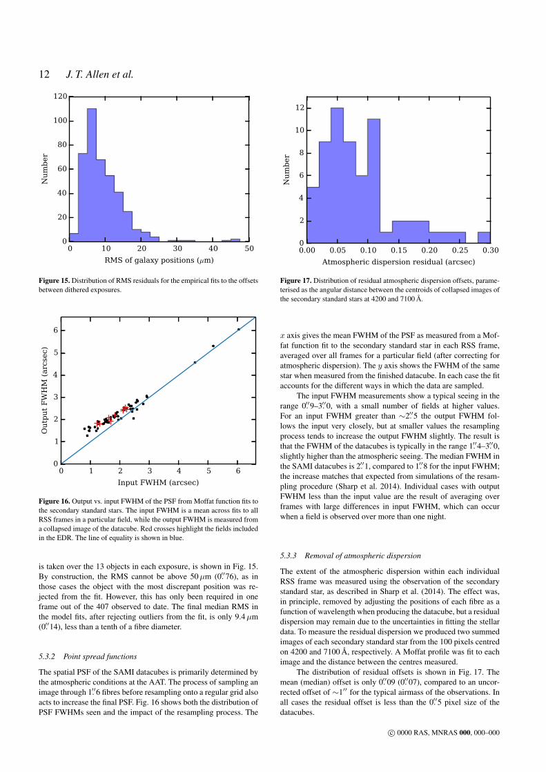
is taken over the 13 objects in each exposure, is shown in Fig. 15.By construction, the RMS cannot be above 50µm (0.′′76), as inthose cases the object with the most discrepant position was re-jected from the fit. However, this has only been required in oneframe out of the 407 observed to date. The final median RMS inthe model fits, after rejecting outliers from the fit, is only 9.4µm(0.′′14), less than a tenth of a fibre diameter.

5.3.2 Point spread functions

The spatial PSF of the SAMI datacubes is primarily determined bythe atmospheric conditions at the AAT. The process of sampling animage through 1.′′6 fibres before resampling onto a regular grid alsoacts to increase the final PSF. Fig. 16 shows both the distribution ofPSF FWHMs seen and the impact of the resampling process. The

0.00 0.05 0.10 0.15 0.20 0.25 0.30

Atmospheric dispersion residual (arcsec)

0

2

4

6

8

10

12

Nu

mb

er

Figure 17. Distribution of residual atmospheric dispersion offsets, parame-terised as the angular distance between the centroids of collapsed images ofthe secondary standard stars at 4200 and 7100 A.

x axis gives the mean FWHM of the PSF as measured from a Mof-fat function fit to the secondary standard star in each RSS frame,averaged over all frames for a particular field (after correcting foratmospheric dispersion). The y axis shows the FWHM of the samestar when measured from the finished datacube. In each case the fitaccounts for the different ways in which the data are sampled.

The input FWHM measurements show a typical seeing in therange 0.′′9–3.′′0, with a small number of fields at higher values.For an input FWHM greater than ∼2.′′5 the output FWHM fol-lows the input very closely, but at smaller values the resamplingprocess tends to increase the output FWHM slightly. The result isthat the FWHM of the datacubes is typically in the range 1.′′4–3.′′0,slightly higher than the atmospheric seeing. The median FWHM inthe SAMI datacubes is 2.′′1, compared to 1.′′8 for the input FWHM;the increase matches that expected from simulations of the resam-pling procedure (Sharp et al. 2014). Individual cases with outputFWHM less than the input value are the result of averaging overframes with large differences in input FWHM, which can occurwhen a field is observed over more than one night.

5.3.3 Removal of atmospheric dispersion

The extent of the atmospheric dispersion within each individualRSS frame was measured using the observation of the secondarystandard star, as described in Sharp et al. (2014). The effect was,in principle, removed by adjusting the positions of each fibre as afunction of wavelength when producing the datacube, but a residualdispersion may remain due to the uncertainties in fitting the stellardata. To measure the residual dispersion we produced two summedimages of each secondary standard star from the 100 pixels centredon 4200 and 7100 A, respectively. A Moffat profile was fit to eachimage and the distance between the centres measured.

The distribution of residual offsets is shown in Fig. 17. Themean (median) offset is only 0.′′09 (0.′′07), compared to an uncor-rected offset of ∼1′′ for the typical airmass of the observations. Inall cases the residual offset is less than the 0.′′5 pixel size of thedatacubes.

c© 0000 RAS, MNRAS 000, 000–000

The SAMI Galaxy Survey: Early Data Release 13

5.3.4 Signal-to-noise ratio

The spaxel size in the SAMI datacubes is a balance between thecompeting requirements of spatial sampling and S/N, as smallerspaxels overlap with fewer fibres and hence have lower S/N. Wehave chosen a relatively small spaxel size in order to conserve asmuch spatial information as possible, with the option to combineadjacent spaxels to increase S/N where necessary.

Fig. 18 shows how the S/N in a SAMI datacube varies as afunction of stellar mass and redshift. In the left panel we plot themean continuum per-pixel S/N across our 0.′′5×0.′′5 spaxels withina circle of 1′′ radius. The S/N in each spaxel is defined as themedian value across the entire wavelength range of the blue arm,where most of the stellar continuum features are found. The medianS/N across these galaxies is 16.5 (10th/90th percentiles: 4.8/33.5).As expected, the S/N is a strong function of stellar mass and red-shift, with high-mass, low-redshift galaxies having the highest S/N.

For IFU observations the amount of spatial information avail-able, after binning if necessary, is often more critical than the peakS/N. The right panel of Fig. 18 illustrates the level of binning thatis required in order to produce spectra with a continuum S/N of atleast 10. We have applied an adaptive binning scheme that com-bines groups of spaxels until it achieves the required S/N (Cappel-lari & Copin 2003). The colour coding shows the number of binsformed in this way for each galaxy, which corresponds to the levelof spatial information that is retained. The median number of binsformed in this way is 93 (10th/90th percentiles: 9/298), indicatingthat for the majority of SAMI galaxies a large amount of spatial in-formation is retained even under strict S/N limits. We note that formost galaxies the number of independent spatial elements is limitedby atmospheric seeing rather than S/N.

The S/N achieved in the emission lines varies enormously de-pending on the emission line flux in each galaxy. Fig. 19 shows theper-spaxel S/N in Hα for the peak Hα flux (left panel), and the frac-tion of spaxels in the field of view for which Hα is detected withS/N>5 (left panel). The Hα flux and S/N were calculated from a si-multaneous Gaussian fit to each strong emission line in each spec-trum, after using a template fit to subtract the stellar continuum(Ho et al. 2014). The median S/N measured in this way is 37.9, butthe distribution ranges from ∼0 to over 500 (10th/90th percentiles:5.8/156.6).

5.3.5 Covariance

As described in Section 3.3, the covariance between nearby spax-els must be taken into account when combining their information.Failure to do so will result in a significant underestimate of the truevariance. To illustrate this point, Fig. 20 shows the effect of covari-ance when summing spectra within a circular aperture of increasingradius. The true uncertainty (square root of variance) is calculatedaccording to:

Varλ =∑i,j

Vari,j,λ + 2∑i,j

∑k<i,l<j

Covi,j,k,l,λ, (1)

where Varλ is the variance of the summed flux as a function ofwavelength, Vari,j,λ is the variance of the (i, j)th spaxel, andCovi,j,k,l,λ is the covariance between the (i, j)th and (k, l)th spax-els. The sum over covariance values runs over all unique pairs ofspaxels.

In contrast, the naive uncertainty, neglecting covariance, is

0 1 2 3 4 5 6 7

Radius (arcsec)

1

2

3

4

5

6

σtr

ue/σ

nai

ve

Figure 20. Ratio of the true uncertainty (including covariance) to the naiveuncertainty (neglecting covariance) when summing all spectra within acircular aperture. Blue and red lines give the ratios for the blue and redAAOmega arms. Solid lines show the median as a function of aperture ra-dius for all galaxy datacubes, while the 10th and 90th percentiles are shownby dashed lines.

found simply from:

Varλ =∑i,j

Vari,j,λ. (2)

Fig. 20 shows how the ratio of the true and naive uncertaintiesvaries as the aperture for summation, and hence number of spaxels,increases. The ratio is plotted as the median across all wavelengthswithin each AAOmega arm and across all galaxies in the sample. Ata radius of 0.′′5 (4 spaxels) the covariance has already increased theuncertainty by a factor of' 1.45. The ratio increases until the aper-ture has a radius of ∼ 2′′ (52 spaxels), at which point it plateaus ata value of' 2.0. At large radii, > 6′′, the ratio increases again dueto the influence of spaxels at the edge of the SAMI field of view.These spaxels have an unusually high covariance because they typ-ically draw their data from only some of the dithered frames, andso have fewer independent input fibres than the spaxels away fromthe edges.

6 CONCLUSIONS

In this paper we have described the contents of the SAMI EarlyData Release (EDR). The EDR consists of a sample of 107 galaxiesselected from the GAMA fields of the full SAMI Galaxy Surveysample. The galaxies in the EDR span a wide range in mass (8.2 <log(M∗/M�) < 11.6) and redshift (0.01 < z < 0.09), and arerepresentative of the GAMA (field and group) regions of the wholesurvey.

Datacubes for each galaxy covering the SAMI field of view(15′′) and the wavelength ranges 3700–5600 and 6300–7400 A,with a 0.′′5 spaxel size, are available for download from the SAMIGalaxy Survey website. As well as the flux cube, the full varianceand covariance information is provided. We emphasise that the co-variance between nearby spaxels should be taken into account inany further analysis, as failure to do so may result in uncertaintiesbeing significantly underestimated.

A quantitative analysis of the SAMI data reduction pipeline

c© 0000 RAS, MNRAS 000, 000–000

14 J. T. Allen et al.

0.00 0.02 0.04 0.06 0.08 0.10

Redshift

7.5

8.0

8.5

9.0

9.5

10.0

10.5

11.0

11.5

12.0

log(M

∗/M

¯)

Continuum S/N2

3

5

10

20

30

50

0.00 0.02 0.04 0.06 0.08 0.10

Redshift

7.5

8.0

8.5

9.0

9.5

10.0

10.5

11.0

11.5

12.0

log(M

∗/M

¯)

Number of bins

1

3

10

30

100

300

Figure 18. Left: Mean continuum S/N within a radius of 1′′ centred on each galaxy, across the stellar mass vs. redshift plane. Right: Number of bins formedby the adaptive binning scheme with a continuum S/N limit of 10, across the same plane.

0.00 0.02 0.04 0.06 0.08 0.10

Redshift

7.5

8.0

8.5

9.0

9.5

10.0

10.5

11.0

11.5

12.0

log(M

∗/M

¯)

S/N at peak flux

3

10

30

100

300

0.00 0.02 0.04 0.06 0.08 0.10

Redshift

7.5

8.0

8.5

9.0

9.5

10.0

10.5

11.0

11.5

12.0

log(M

∗/M

¯)

Fraction of spaxels with S/N>5

10-3

10-2

10-1

100

Figure 19. Left: S/N of Hα emission in the spaxel with the peak Hα flux, across the stellar mass vs. redshift plane. Right: Fraction of spaxels within the fieldof view for which Hα is detected with S/N>5.

has shown it to be performing to a very high standard at all stages.Key quality metrics include:

(i) Cross-talk between adjacent fibres on the CCD is typically∼0.5 per cent.

(ii) Flat-fielding accuracy of 0.5–1 per cent in the blue arm, ris-ing to ∼2 per cent at wavelengths below 4000 A, and 0.3–0.4 percent in the red.

(iii) Residuals in the wavelength calibration at a level of 0.1 pix-els (RMS) or better.

(iv) Uncertainties in the throughput calibration less than1 per cent.

(v) After sky subtraction, median residual sky line fluxes of 0.8per cent (blue arm) and 0.9 per cent (red arm), relative to the un-subtracted flux.

(vi) Continuum residuals are typically 1.2 per cent (blue arm)and 0.9 per cent (red arm) of the sky level, rising to ∼5 per cent insome fibres.

(vii) In terms of the g − r colour, flux calibration that agreeswith existing photometric catalogues to within 4.3 per cent, witha mean offset of 4.1 per cent (with the SAMI observations beingredder).

(viii) An absolute flux calibration with a mean offset of 4.4 percent (with the SAMI observations being brighter) relative to SDSSphotometry, with a scatter of 28 per cent.

(ix) Multiple dithered exposures for each field are aligned witha median accuracy of 9.4µm, less than a tenth of a fibre diameter.

(x) The observed PSF in the final datacubes is primarily deter-mined by the atmospheric conditions, with a median seeing FWHMof 2.′′1.

(xi) The effects of atmospheric dispersion removed from thedatacubes with a mean residual between images at different wave-lengths of 0.′′09.

(xii) A median per-pixel continuum S/N in the central 0.′′5×0.′′5spaxels of 16.5, with 10th/90th percentiles of 4.8/33.5.

c© 0000 RAS, MNRAS 000, 000–000

The SAMI Galaxy Survey: Early Data Release 15

ACKNOWLEDGMENTS

The SAMI Galaxy Survey is based on observations made at theAnglo-Australian Telescope. The Sydney-AAO Multi-object In-tegral field spectrograph (SAMI) was developed jointly by theUniversity of Sydney and the Australian Astronomical Observa-tory. The SAMI input catalogue is based on data taken from theSloan Digital Sky Survey, the GAMA Survey and the VST AT-LAS Survey. The SAMI Galaxy Survey is funded by the Aus-tralian Research Council Centre of Excellence for All-sky Astro-physics (CAASTRO), through project number CE110001020, andother participating institutions. The SAMI Galaxy Survey websiteis http://sami-survey.org/ .

GAMA is a joint European-Australasian project based arounda spectroscopic campaign using the Anglo-Australian Telescope.The GAMA input catalogue is based on data taken from theSloan Digital Sky Survey and the UKIRT Infrared Deep Sky Sur-vey. Complementary imaging of the GAMA regions is being ob-tained by a number of independent survey programs includingGALEX MIS, VST KiDS, VISTA VIKING, WISE, Herschel-ATLAS, GMRT and ASKAP providing UV to radio coverage.GAMA is funded by the STFC (UK), the ARC (Australia), theAAO, and the participating institutions. The GAMA website ishttp://www.gama-survey.org/ .

JTA acknowledges the award of an Australian ResearchCouncil (ARC) Super Science Fellowship (FS110200013). SMCacknowledges the support of an ARC Future Fellowship(FT100100457). MSO acknowledges the funding support from theARC through a Super Science Fellowship (FS110200023). LC ac-knowledges support under the ARC Discovery Projects fundingscheme (DP130100664).

This research made use of Astropy, a community-developedcore Python package for Astronomy (Astropy Collaboration et al.2013).

References

Allen J. T., et al., 2014, Astrophysics Source Code Library, ascl:1407.006Astropy Collaboration et al., 2013, A&A, 558, A33Baldry I. K., et al., 2012, MNRAS, 421, 621Bland-Hawthorn J., et al., 2011, Optics Express, 19, 2649Brough S., et al., 2013, MNRAS, 435, 2903Bryant J. J., O’Byrne J. W., Bland-Hawthorn J., Leon-Saval S. G., 2011,

MNRAS, 415, 2173Bryant J. J., Bland-Hawthorn J., Fogarty L. M. R., Lawrence J. S., Croom

S. M., 2014a, MNRAS, 438, 869Bryant J. J., et al., 2014b, submittedCappellari M., Copin Y., 2003, MNRAS, 342, 345Cappellari M., Emsellem E., 2004, PASP, 116, 138Cappellari M., et al., 2011a, MNRAS, 413, 813Cappellari M., et al., 2011b, MNRAS, 416, 1680Childress M. J., Vogt F. P. A., Nielsen J., Sharp R. G., 2014, Astrophysics

and Space Science, 349, 617Colless M., et al., 2001, MNRAS, 328, 1039Croom S. M., et al., 2012, MNRAS, 421, 872Driver S. P., et al., 2009, Astronomy and Geophysics, 50, 12Driver S. P., et al., 2011, MNRAS, 413, 971Flores H., Hammer F., Puech M., Amram P., Balkowski C., 2006, A&A,

455, 107Fogarty L. M. R., et al., 2012, ApJ, 761, 169Fogarty L. M. R., et al., 2014, MNRAS accepted, arXiv:1406.3899Fruchter A. S., Hook R. N., 2002, PASP, 114, 144Genzel R., et al., 2008, ApJ, 687, 59Hill D. T., et al., 2011, MNRAS, 412, 765

Ho I.-T., et al., 2014, submitted, arXiv:1407.2411Hogg D. W., Baldry I. K., Blanton M. R., Eisenstein D. J., 2002, ArXiv

e-prints, astro-ph/0210394Hopkins A. M., et al., 2003, ApJ, 599, 971Horne K., 1986, PASP, 98, 609Husemann B., et al., 2013, A&A, 549, A87Jones D. H., et al., 2009, MNRAS, 399, 683Kelvin L. S., et al., 2012, MNRAS, 421, 1007Kron R. G., 1980, ApJS, 43, 305Lara-Lopez M. A., et al., 2013, MNRAS, 434, 451Lewis I., et al., 2002, MNRAS, 334, 673Mannucci F., Cresci G., Maiolino R., Marconi A.,Gnerucci A., 2010, MN-

RAS, 408, 2115Pasquini L., et al., 2002, The Messenger, 110, 1Pence W. D., Chiappetti L., Page C. G., Shaw R. A., Stobie E., 2010,

A&A, 524, A42Petrosian V., 1976, ApJ, 209, L1Richards S. N., et al., 2014, submittedSanchez S. F., et al., 2012, A&A, 538, A8Shanks T., et al., 2013, The Messenger, 154, 38Sharp R., Birchall M. N., 2010, PASA, 27, 91Sharp R. G., Bland-Hawthorn J., 2010, ApJ, 711, 818Sharp R., Parkinson H., 2010, MNRAS, 408, 2495Sharp R., et al., 2006, in Society of Photo-Optical Instrumentation Engi-

neers (SPIE) Conference Series Vol. 6269Sharp R., Brough S., Cannon R. D., 2013, MNRAS, 428, 447Sharp R., et al., 2014, submittedShen J., Vanden Berk D. E., Schneider D. P., Hall P. B., 2008, AJ, 135,

928Taylor E. N., et al., 2011, MNRAS, 418, 1587Tonry J. L., Blakeslee J. P., Ajhar E. A., Dressler A., 2000, ApJ, 530, 625Wijesinghe D. B., et al., 2012, MNRAS, 423, 3679Yang Y., et al., 2008, A&A, 477, 789York D. G., et al., 2000, AJ, 120, 1579

APPENDIX A: GALAXIES IN THE SAMI EDR

Table A1 gives information about the galaxies included in theSAMI Galaxy Survey EDR.

c© 0000 RAS, MNRAS 000, 000–000

16 J. T. Allen et al.

Table A1. Galaxies included in the SAMI EDR. For each galaxy we list: the galaxy name; J2000 coordinates (decimal degrees); extinction-corrected r-bandmagnitudes measured using the Petrosian (‘petro’; Petrosian 1976) and Kron (‘auto’; Kron 1980) systems (Hill et al. 2011); redshifts corrected (‘tonry’; Tonryet al. 2000; Baldry et al. 2012) and uncorrected (‘spec’) for large-scale flow; r-band rest-frame absolute magnitude; r-band effective radius (Re) along majoraxis (arcsec; Kelvin et al. 2012); r-band surface brightness (mag arcsec−2) within Re, at Re and at 2Re; ellipticity and position angle (deg), measured in ther band; logarithm of stellar mass (M�; Taylor et al. 2011; Bryant et al. 2014b); g− i colour from Kron magnitudes; Galactic extinction in the g band; GAMAcatalogue ID; SAMI Galaxy Survey priority (8: main sample, 4: high-mass fillers, 3: other fillers); field in which the galaxy was observed; and URLs for theblue and red datacubes. Only the first five entries are printed; the full table is available as Supporting Information with the online version of the paper, or onthe SAMI Galaxy Survey website at http://sami-survey.org/edr/data/SAMI EarlyDataRelease.txt .

Name R.A. Dec. rpetro rauto ztonry zspec Mr Re

J084445.41+021107.8 131.1892 +2.1855 15.781 15.801 0.07548 0.07444 −21.96 4.17J084458.94+020305.9 131.2456 +2.0517 16.167 16.153 0.05193 0.05091 −20.70 1.94J084459.22+022834.8 131.2468 +2.4763 15.981 15.942 0.05064 0.04962 −20.88 6.76J084517.68+021650.0 131.3237 +2.2806 17.036 17.021 0.05106 0.05004 −19.81 2.87J084531.79+022833.1 131.3825 +2.4759 15.311 15.188 0.07756 0.07651 −22.64 6.76

Table A1 – continued

〈µ(Re)〉 µ(Re) µ(2Re) ellip. PA M∗ g − i Ag CATID SURV SAMI Tile no.

22.19 21.40 23.00 0.5116 3.28 10.95 1.30 0.244 386268 8 Y13SAR1 P005 09T00923.04 20.54 22.17 0.2758 93.58 10.26 1.00 0.316 345820 8 Y13SAR1 P005 09T00921.46 22.49 24.06 0.5711 8.36 10.36 1.02 0.154 517164 8 Y13SAR1 P005 09T00920.49 22.58 24.18 0.0120 11.30 10.09 1.22 0.212 417486 8 Y13SAR1 P005 09T00920.13 22.43 24.01 0.2140 160.43 11.24 1.31 0.165 517205 8 Y13SAR1 P005 09T009

Table A1 – continued

Blue cube

http://sami-survey.org/edr/data/386268/386268 blue 7 Y13SAR1 P005 09T009.fits.gzhttp://sami-survey.org/edr/data/345820/345820 blue 7 Y13SAR1 P005 09T009.fits.gzhttp://sami-survey.org/edr/data/517164/517164 blue 7 Y13SAR1 P005 09T009.fits.gzhttp://sami-survey.org/edr/data/417486/417486 blue 7 Y13SAR1 P005 09T009.fits.gzhttp://sami-survey.org/edr/data/517205/517205 blue 7 Y13SAR1 P005 09T009.fits.gz

Table A1 – continued

Red cube

http://sami-survey.org/edr/data/386268/386268 red 7 Y13SAR1 P005 09T009.fits.gzhttp://sami-survey.org/edr/data/345820/345820 red 7 Y13SAR1 P005 09T009.fits.gzhttp://sami-survey.org/edr/data/517164/517164 red 7 Y13SAR1 P005 09T009.fits.gzhttp://sami-survey.org/edr/data/417486/417486 red 7 Y13SAR1 P005 09T009.fits.gzhttp://sami-survey.org/edr/data/517205/517205 red 7 Y13SAR1 P005 09T009.fits.gz

c© 0000 RAS, MNRAS 000, 000–000