Although topology was recognized by Gauss and Maxwell to play a pivotal role in the formulation of electromagnetic boundary value problems, it is a largely unexploited tool for field computation. The development of algebraic topology since Maxwell provides a framework for linking data structures, algorithms, and computation to topological aspects of three-dimensional electromagnetic boundary value problems. This book attempts to expose the link between Maxwell and a modern approach to algorithms. The first chapters lay out the relevant facts about homology and coho- mology, stressing their interpretations in electromagnetism. These topological structures are subsequently tied to variational formulations in electromagnet- ics, the finite element method, algorithms, and certain aspects of numerical linear algebra. A recurring theme is the formulation of and algorithms for the problem of making branch cuts for computing magnetic scalar potentials and eddy currents. An appendix bridges the gap between the material presented and standard expositions of differential forms, Hodge decompositions, and tools for realizing representatives of homology classes as embedded manifolds.

Welcome message from author
This document is posted to help you gain knowledge. Please leave a comment to let me know what you think about it! Share it to your friends and learn new things together.
Transcript

Although topology was recognized by Gauss and Maxwell to play a pivotal rolein the formulation of electromagnetic boundary value problems, it is a largelyunexploited tool for field computation. The development of algebraic topologysince Maxwell provides a framework for linking data structures, algorithms,and computation to topological aspects of three-dimensional electromagneticboundary value problems. This book attempts to expose the link betweenMaxwell and a modern approach to algorithms.
The first chapters lay out the relevant facts about homology and coho-mology, stressing their interpretations in electromagnetism. These topologicalstructures are subsequently tied to variational formulations in electromagnet-ics, the finite element method, algorithms, and certain aspects of numericallinear algebra. A recurring theme is the formulation of and algorithms for theproblem of making branch cuts for computing magnetic scalar potentials andeddy currents. An appendix bridges the gap between the material presentedand standard expositions of differential forms, Hodge decompositions, andtools for realizing representatives of homology classes as embedded manifolds.


Mathematical Sciences Research InstitutePublications
48
Electromagnetic Theory and Computation
A Topological Approach

Mathematical Sciences Research Institute Publications
1 Freed/Uhlenbeck: Instantons and Four-Manifolds, second edition
2 Chern (ed.): Seminar on Nonlinear Partial Differential Equations
3 Lepowsky/Mandelstam/Singer (eds.): Vertex Operators in Mathematics and Physics
4 Kac (ed.): Infinite Dimensional Groups with Applications5 Blackadar: K-Theory for Operator Algebras, second edition
6 Moore (ed.): Group Representations, Ergodic Theory, Operator Algebras, and
Mathematical Physics
7 Chorin/Majda (eds.): Wave Motion: Theory, Modelling, and Computation8 Gersten (ed.): Essays in Group Theory
9 Moore/Schochet: Global Analysis on Foliated Spaces
10–11 Drasin/Earle/Gehring/Kra/Marden (eds.): Holomorphic Functions and Moduli
12–13 Ni/Peletier/Serrin (eds.): Nonlinear Diffusion Equations and Their Equilibrium States14 Goodman/de la Harpe/Jones: Coxeter Graphs and Towers of Algebras
15 Hochster/Huneke/Sally (eds.): Commutative Algebra
16 Ihara/Ribet/Serre (eds.): Galois Groups over Q
17 Concus/Finn/Hoffman (eds.): Geometric Analysis and Computer Graphics
18 Bryant/Chern/Gardner/Goldschmidt/Griffiths: Exterior Differential Systems
19 Alperin (ed.): Arboreal Group Theory
20 Dazord/Weinstein (eds.): Symplectic Geometry, Groupoids, and Integrable Systems21 Moschovakis (ed.): Logic from Computer Science
22 Ratiu (ed.): The Geometry of Hamiltonian Systems
23 Baumslag/Miller (eds.): Algorithms and Classification in Combinatorial Group Theory
24 Montgomery/Small (eds.): Noncommutative Rings25 Akbulut/King: Topology of Real Algebraic Sets
26 Judah/Just/Woodin (eds.): Set Theory of the Continuum
27 Carlsson/Cohen/Hsiang/Jones (eds.): Algebraic Topology and Its Applications28 Clemens/Kollar (eds.): Current Topics in Complex Algebraic Geometry
29 Nowakowski (ed.): Games of No Chance
30 Grove/Petersen (eds.): Comparison Geometry
31 Levy (ed.): Flavors of Geometry32 Cecil/Chern (eds.): Tight and Taut Submanifolds
33 Axler/McCarthy/Sarason (eds.): Holomorphic Spaces
34 Ball/Milman (eds.): Convex Geometric Analysis
35 Levy (ed.): The Eightfold Way36 Gavosto/Krantz/McCallum (eds.): Contemporary Issues in Mathematics Education
37 Schneider/Siu (eds.): Several Complex Variables
38 Billera/Bjorner/Green/Simion/Stanley (eds.): New Perspectives in GeometricCombinatorics
39 Haskell/Pillay/Steinhorn (eds.): Model Theory, Algebra, and Geometry
40 Bleher/Its (eds.): Random Matrix Models and Their Applications
41 Schneps (ed.): Galois Groups and Fundamental Groups42 Nowakowski (ed.): More Games of No Chance
43 Montgomery/Schneider (eds.): New Directions in Hopf Algebras
44 Buhler/Stevenhagen (eds.): Algorithmic Number Theory
45 Jensen/Ledet/Yui: Generic Polynomials: Constructive Aspects of the Inverse GaloisProblem
46 Rockmore/Healy (eds.): Modern Signal Processing
47 Uhlmann (ed.): Inside Out: Inverse Problems and Applications
48 Gross/Kotiuga: Electromagnetic Theory and Computation: A Topological Approach
Volumes 1–4 and 6–27 are published by Springer-Verlag

Electromagnetic Theoryand Computation:
A Topological Approach
Paul W. GrossMSRI and HP/Agilent
P. Robert KotiugaBoston University

Series EditorSilvio LevyMathematical Sciences
Paul Gross Research [email protected] 17 Gauss Way
Berkeley, CA 94720United States
P. Robert KotiugaDepartment of Electrical MSRI Editorial Committeeand Computer Engineering Hugo Rossi (chair)
Boston University Alexandre Chorin8 Saint Mary’s Street Silvio LevyBoston, MA 02215 Jill MesirovUnited States Robert [email protected] Peter Sarnak
The Mathematical Sciences Research Institute wishes to acknowledge support bythe National Science Foundation. This material is based upon work supported by
NSF Grant 9810361.
published by the press syndicate of the university of cambridge
The Pitt Building, Trumpington Street, Cambridge, United Kingdom
cambridge university press
The Edinburgh Building, Cambridge CB2 2RU, UK40 West 20th Street, New York, NY 10011-4211, USA
477 Williamstown Road, Port Melbourne, VIC 3207, AustraliaRuiz de Alarcon 13, 28014 Madrid, Spain
Dock House, The Waterfront, Cape Town 8001, South Africa
http://www.cambridge.org
c© Mathematical Sciences Research Institute 2004
Printed in the United States of America
A catalogue record for this book is available from the British Library.
Library of Congress Cataloging in Publication data available
ISBN 0 521 801605 hardback

Table of Contents
Preface ix
Introduction 1
Chapter 1. From Vector Calculus to Algebraic Topology 71A Chains, Cochains and Integration 71B Integral Laws and Homology 101C Cohomology and Vector Analysis 151D Nineteenth-Century Problems Illustrating the First and Second
Homology Groups 181E Homotopy Versus Homology and Linking Numbers 251F Chain and Cochain Complexes 281G Relative Homology Groups 321H The Long Exact Homology Sequence 371I Relative Cohomology and Vector Analysis 411J A Remark on the Association of Relative Cohomology Groups with
Perfect Conductors 46
Chapter 2. Quasistatic Electromagnetic Fields 492A The Quasistatic Limit Of Maxwell’s Equations 492B Variational Principles For Electroquasistatics 632C Variational Principles For Magnetoquasistatics 702D Steady Current Flow 802E The Electromagnetic Lagrangian and Rayleigh Dissipation Functions 89
Chapter 3. Duality Theorems for Manifolds With Boundary 993A Duality Theorems 993B Examples of Duality Theorems in Electromagnetism 1013C Linking Numbers, Solid Angle, and Cuts 1123D Lack of Torsion for Three-Manifolds with Boundary 117
Chapter 4. The Finite Element Method and Data Structures 1214A The Finite Element Method for Laplace’s Equation 1224B Finite Element Data Structures 1274C The Euler Characteristic and the Long Exact Homology Sequence 138
vii

viii TABLE OF CONTENTS
Chapter 5. Computing Eddy Currents on Thin Conductors with ScalarPotentials 141
5A Introduction 1415B Potentials as a Consequence of Ampere’s Law 1425C Governing Equations as a Consequence of Faraday’s Law 1475D Solution of Governing Equations by Projective Methods 1475E Weak Form and Discretization 150
Chapter 6. An Algorithm to Make Cuts for Magnetic Scalar Potentials 1596A Introduction and Outline 1596B Topological and Variational Context 1616C Variational Formulation of the Cuts Problem 1686D The Connection Between Finite Elements and Cuts 1696E Computation of 1-Cocycle Basis 1726F Summary and Conclusions 180
Chapter 7. A Paradigm Problem 1837A The Paradigm Problem 1837B The Constitutive Relation and Variational Formulation 1857C Gauge Transformations and Conservation Laws 1917D Modified Variational Principles 1977E Tonti Diagrams 207
Mathematical Appendix: Manifolds, Differential Forms, Cohomology,Riemannian Structures 215
MA-A Differentiable Manifolds 216MA-B Tangent Vectors and the Dual Space of One-Forms 217MA-C Higher-Order Differential Forms and Exterior Algebra 220MA-D Behavior of Differential Forms Under Mappings 223MA-E The Exterior Derivative 226MA-F Cohomology with Differential Forms 229MA-G Cochain Maps Induced by Mappings Between Manifolds 231MA-H Stokes’ Theorem, de Rham’s Theorems and Duality Theorems 232MA-I Existence of Cuts Via Eilenberg–MacLane Spaces 240MA-J Riemannian Structures, the Hodge Star Operator and an Inner
Product for Differential Forms 243MA-K The Operator Adjoint to the Exterior Derivative 249MA-L The Hodge Decomposition and Ellipticity 252MA-M Orthogonal Decompositions of p-Forms and Duality Theorems 253
Bibliography 261
Summary of Notation 267
Examples and Tables 273
Index 275

Preface
The authors are long-time fans of MSRI programs and monographs, and arethrilled to be able to contribute to this series. Our relationship with MSRIstarted when Paul Gross was an MSRI/Hewlett-Packard postdoctoral fellowand had the good fortune of being encouraged by Silvio Levy to coauthor amonograph. Silvio was there when we needed him, and it is in no way an under-statement to say that the project would never have been completed without hissupport.
The material of this monograph is easily traced back to our Ph.D. theses,papers we wrote, and courses taught at Boston University over the years. Ourapologies to anyone who feels slighted by a minimally updated bibliography.Reflecting on how the material of this monograph evolved, we would like tothank colleagues who have played a supporting role over the decades. Amongthem are Alain Bossavit, Peter Caines, Roscoe Giles, Robert Hermann, LauriKettunen, Isaak Mayergoyz, Peter Silvester, and Gilbert Strang. The authors arealso indebted to numerous people who read through all or part of the manuscript,produced numerous comments, and provided all sorts of support. In particular,Andre Nicolet, Jonathan Polimeni, and Saku Suuriniemi made an unusuallythorough effort to review the draft.
Paul Gross would like to acknowledge Nick Tufillaro at Hewlett-Packard andAgilent Technologies for mentoring him throughout his post-doc at MSRI. TimDere graciously provided his time and expertise for illustrations. This book couldnot have happened without help and encouragement from Tanya.
Robert Kotiuga is grateful to the students taking his courses at Boston Uni-versity, to Nevine, Michele, Madeleine, Peter and Helen for their support, and toBoston University for granting him a leave while the book was in its final stages.
Paul Gross and Robert KotiugaAugust 2003
ix


We are here led to considerations belonging to the Geometry of Position, asubject which, though its importance was pointed out by Leibnitz andillustrated by Gauss, has been little studied.
James Clerk Maxwell, A Treatise on Electricity and Magnetism, 1891
Introduction
The title of this book makes clear that we are after connections between elec-tromagnetics, computation and topology. However, connections between thesethree fields can mean different things to different people. For a modern engineer,computational electromagnetics is a well-defined term and topology seems to bea novel aspect. To this modern engineer, discretization methods for Maxwell’sequations, finite element methods, numerical linear algebra and data structuresare all part of the modern toolkit for effective design and topology seems to havetaken a back seat. On the other hand, to an engineer from a half-century ago,the connection between electromagnetic theory and topology would be consid-ered “obvious” by considering Kirchhoff’s laws and circuit theory in the lightof Maxwell’s electromagnetic theory. To this older electrical engineer, topologywould be considered part of the engineer’s art with little connection to computa-tion beyond what Maxwell and Kirchhoff would have regarded as computation.A mathematician could snicker at the two engineers and proclaim that all is triv-ial once one gets to the bottom of algebraic topology. Indeed the present bookcan be regarded as a logical consequence for computational electromagnetismof Eilenberg and Steenrod’s Foundations of Algebraic Topology [ES52], Whit-ney’s Geometric Integration Theory [Whi57] and some differential topology. Ofcourse, this would not daunt the older engineer who accomplished his task beforemathematicians and philosophers came in to lay the foundations.
The three points of view described above expose connections between pairsof each of the three fields, so it is natural to ask why it is important to put allthree together in one book. The answer is stated quite simply in the context ofthe three characters mentioned above. In a modern “design automation” envi-ronment, it is necessary to take the art of the old engineer, reduce it to a scienceas much as possible, and then turn that into a numerical computation. For thepurposes of computation, we need to feed a geometric model of a device suchas a motor or circuit board, along with material properties, to a program whichexploits algebraic topology in order to extract a simple circuit model from ahorrifically complicated description in terms of partial differential equations andboundary value problems. Cohomology and Hodge theory on manifolds withboundary are the bridge between Maxwell’s equations and the lumped param-eters of circuit theory, but engineers need software that can reliably make this
1

2 INTRODUCTION
connection in an accurate manner. This book exploits developments in alge-braic topology since the time of Maxwell to provide a framework for linking datastructures, algorithms, and computation to topological aspects of 3-dimensionalelectromagnetic boundary value problems. More simply, we develop the link be-tween Maxwell and a modern topological approach to algorithms for the analysisof electromagnetic devices.
To see why this is a natural evolution, we should review some facts fromrecent history. First, there is Moore’s law, which is not a physical law but theobservation that computer processing power has been doubling every eighteenmonths. In practical terms this means that in the year 2003 the video gameplayed by five-year-old playing had the same floating-point capability as thelargest supercomputer 15 years earlier. Although the current use of the term“computer” did not exist in the English language before 1950, Moore’s law canbe extrapolated back in time to vacuum tube computers, relay computers, andmechanical computing machines of the 1920’s. Moving forward in time, theeconomics of building computers will bring this exponential increase to a haltbefore physics predicts the demise of Moore’s law, but we are confident this trendwill continue for at least another decade. Hence we should consider scientificcomputing and computational electromagnetics in this light.
The second set of facts we need to review concern the evolution of the toolsused to solve elliptic boundary value problems. This story starts with Dirichlet’sprinciple, asserting the existence of a minimizer for a quadratic functional whoseEuler–Lagrange equation is Laplace’s equation. Riemann used it effectively inhis theory of analytic functions, but Weierstrass later put it into disrepute withhis counterexamples. Hilbert rescued it with the concept of a minimizing se-quence, and in the process modern functional analysis took a great step for-ward. From the point of view of finite element analysis, the story really startswith Courant, who in the 1920’s suggested triangulating the underlying domain,using piecewise-polynomial trial functions for Ritz’s method and producing aminimizing sequence by subdividing the triangulation. Courant had a construc-tive proof in mind, but three decades later his idea was the basis of the finiteelement method. Issues of adaptive mesh refinement can be interpreted as anattempt to produce a best approximation for a fixed number of degrees of free-dom, as the number of degrees of freedom increase. In the electrical engineeringof the 1960’s, the finite element method started making an impact in the areaof two-dimensional static problems that could be formulated in terms of a scalarpotential or stream function. With the development of computer graphics in the1970’s, electrical engineers were beginning to turn their attention to the represen-tation of vector fields, three-dimensional problems, and the adaptive generationof finite element meshes. At the same time, it is somewhat unfortunate thatthe essence of electromagnetic theory seen in Faraday and Maxwell’s admirablequalitative spatial reasoning was lost under the vast amounts of numerical datagenerated by computer. In the 1980’s came the realization that differential formmethods could be translated to the discrete setting and that the hard work hadalready been done by Andre Weil and Hassler Whitney in the 1950’s, but this

INTRODUCTION 3
point of view was a little slow to catch on. Technology transfer from mathemat-ics to engineering eventually happened, since all of this mathematics from the1950’s was set in terms of simplicial complexes which fit hand in glove with thedata structures of finite element analysis.
Before outlining the book in detail, there is one more observation to makeabout the process of automating the topological aspects that were once consid-ered to be the engineer’s art. Not only has the exponential increase in computingpower given us the means to tackle larger and higher dimensional problems, butit has fundamentally changed the way we interact with computers. It took lessthan twenty years from “submitting a job” with a stack of punched cards at theuniversity computing center to simulating an electromagnetic field in a personalvirtual reality environment. With the continuing evolution of three-dimensional,real-time video games, we are assured of improved environments for having com-puters deal with the topological aspects of electromagnetic design. The taskat hand is to identify the interactions between electromagnetics and algebraictopology that can have the greatest impact on formalizing the design engineer’sintuition so that computers can be integrated more effectively into the designprocess.
Outline of Book. Chapter 1 develops homology and cohomology in the contextof vector calculus, while suppressing the formalism of exterior algebra and dif-ferential forms. This enables practicing engineers to appreciate the relevanceof the material with minimal effort. Although Gauss, Helmholtz, Kirchhoffand Maxwell recognized that topology plays a pivotal role in the formulationof electromagnetic boundary value problems, it is still a largely unexploited toolin problem formulation and computational methods for electromagnetic fields.Most historians agree that Poincare and Betti wrote the seminal papers on whatis now known as algebraic topology. However, it is also clear that they stoodon the shoulders of Riemann and Listing. A glimpse into the first chapter of[Max91] shows that these same giants were under the feet of Maxwell. Corre-spondence between Maxwell and Tait reveals that Maxwell consciously avoidedboth Grassmann’s exterior algebra and Hamilton’s quaternions as a formalism forelectromagnetism in order to avoid ideological debates. Credit is usually given toOliver Heaviside for fitting Maxwell’s equations into a notation accessible to en-gineers. Hence it is fair to say that the wonderful insights into three-dimensionaltopology found in Maxwell’s treatise have never been exploited effectively by en-gineers. Thus our first chapter is a tunnel from some of the heuristic topologicalinstincts of engineers to the commutative algebraic structures that can be ex-tracted from the data structures found in electromagnetic field analysis software.A mathematician would make this all rigorous by appealing to the formalism ofdifferentiable manifolds and differential forms. We leave the reader the luxuryof seeing how this happens in a Mathematical Appendix.
Chapter 2 underlines the notion of a quasistatic electromagnetic field in thecontext Maxwell’s equations. Quasistatics is an engineer’s ticket to ellipticboundary value problems, variational principles leading to numerical algorithms,and the finite element method. We make certain physical assumptions in order

4 INTRODUCTION
to formulate the quasistatic problem, and the reader gets to see how circuit the-ory in the sense of Kirchhoff arises in the context of quasistatic boundary valueproblems. Besides promoting the boundary value problem point of view, thevariational principles discussed in chapter 2 tie duality theorems for manifoldswith boundary to the lumped parameters of circuit theory.
Having had a intuitive glimpse into the uses of duality theorems for manifoldswith boundary in the first two chapters, Chapter 3 goes on to formalize some ofthe underlying ideas. After presenting the traditional Poincare and Lefschetz du-ality theorems in the context of electromagnetics and circuit theory, we move toAlexander duality and present it in the context of linking numbers and magneticscalar potentials. This approach is closest to Gauss’ understanding of the mat-ter and is completely natural in the context of magnetoquasistatics. Finally, forsubsets of three-dimensional Euclidean space that have a continuous retractioninto their interiors, we show that the absolute and relative (modulo boundary)homology and cohomology groups, as commutative groups, are torsion-free. Thisis significant for two reasons. First, it tells us why coming up with simple ex-amples of torsion phenomena in three dimensions is a bit tricky, and second, itpaves the way to using integer arithmetic in algorithms which would otherwisebe susceptible to rounding error if implemented with floating point operations.With this result we are ready to return to the primary concerns of the engineer.
In Chapter 4 we finally arrive at the finite element method. It is introducedin the context of Laplace’s equation and a simplicial mesh. The simplicial tech-niques used in topology are shown to translate into effective numerical algorithmsthat are naturally phrased in terms of the data structures encountered in finiteelement analysis. Although this opens the door to many relatively recent devel-opments in computational electromagnetics, we focus on how the structures ofhomology and cohomology arise in the context of finite element algorithms forcomputing 3-dimensional electric and magnetic fields. In this way, the effective-ness of algebraic topology can be appreciated in a well-studied computationalsetting. Along the way we also get to see how the Euler characteristic is aneffective tool in the analysis of algorithms.
One of the main strengths of the book comes to center stage in Chapter 5.This chapter addresses the problem of coupling magnetic scalar potentials inmultiply-connected regions to stream functions which describe currents confinedto conducting surfaces. This problem is considered in detail and the topolog-ical aspects are followed from the problem formulation stage through to thematrix equations arising from the finite element discretization. In practice thisproblem arises in non-destructive evaluation of aircraft wings, pipes, and otherplaces. This problem is unique in that it is a three-dimensional magnetoqua-sistatic problem which admits a formulation solely in terms of scalar potentials,yet the topological aspects can be formulated in full generality while the over-all formulation is sufficiently simple that it can be presented concisely. Thischapter builds on all of the concepts developed in previous chapters, and is anideal playground for illustrating how the tools of homological algebra (long ex-act sequences, duality theorems, etc.) are essential from problem formulation tointerpretation of the resulting matrix equations.

INTRODUCTION 5
Chapter 5 is self-contained except that one fundamental issue is acknowledgedbut sidestepped up to this point in the book. That issue is computation of cutsfor magnetic scalar potentials. This is a deep issue since the simplest generaldefinition of a cut is a realization, as an embedded orientable manifold withboundary, of an element of the second homology group of a region modulo itsboundary. Poincare and Maxwell took the existence of cuts for granted, and itwas Pontryagin and Thom who, in different levels of generality, pointed out theneed for an existence proof and gave a general framework for realizing homologyclasses as manifolds in the case that there is such a realization. It is ironicthat historically, this question was avoided until the tools for its resolution weredeveloped. For our purposes, an existence proof is given in the MathematicalAppendix, and the actual algorithm for computing a set of cuts realizing a basisfor the second homology group is given in chapter six.
Chapter 6 bridges the gap between the existence of cuts and their realiza-tion as piecewise-linear manifolds which are sub-complexes of a finite elementmesh (considered as a simplicial complex). Any algorithm to perform this taskis useful only if some stringent complexity requirements are met. Typically, ona given mesh, a magnetic scalar potential requires about an order of magnitudeless work to compute than computing the magnetic field directly. Hence if thecomputation of cuts is not comparable to the computation of a static solution ofa scalar potential subject to linear constitutive laws, the use of scalar potentialsin multiply-connected regions is not feasible for time-varying and/or nonlinearproblems. We present an algorithm that involves the formulation and finiteelement solution of a Poisson-like equation, and additional algorithms that in-volve only integer arithmetic. We then have a favorable expression of the overallcomplexity in terms of a familiar finite element solution and the reordering andsolution of a large sparse integer matrix equation arising for homology compu-tation. This fills in the difficult gap left over from Chapter 5.
Chapter 7, the final chapter, steps back and considers the techniques of ho-mological algebra in the context of the variational principles used in the finiteelement analysis of quasistatic electromagnetic fields. The message of this chap-ter is that the formalism of homology, and cohomology theory via differentialform methods, are essential for revealing the conceptual elegance of variationalmethods in electromagnetism as well as providing a framework for software devel-opment. In order to get this across, a paradigm variational problem is formulatedwhich includes as special cases all of the variational principles considered in ear-lier chapters. All the topological aspects considered in earlier chapters are thenseen in the light of the homology and cohomology groups arising in the analysisof this paradigm problem. Because the paradigm problem is n-dimensional, thischapter no longer emphasizes the more visual and intuitive aspects, but exploitsthe formalism of differential forms in order to make connections to Hodge the-ory on manifolds with boundary, and variational methods for quasilinear ellipticpartial differential equations. The engineer’s topological intuition has now beenobscured, but we gain a paradigm variational problem for which topological as-pects which lead to circuit models are reduced by Whitney form discretizationto computations involving well-understood algorithms.

6 INTRODUCTION
The Mathematical Appendix serves several purposes. First, it contains resultsthat make the book more mathematically self-contained. These results make thealgebraic aspects accessible to the uninitiated, tie differential forms to cohomol-ogy, make clear what aspects of cohomology theory depend on the metric orconstitutive law, and which do not. Second, certain results, such as the proof ofthe existence of cuts, are presented. This existence proof points to an algorithmfor finding cuts, but involves tools from algebraic topology not found in intro-ductory treatments. Having this material in an appendix makes the chapters ofthe book more independent.
Having stated the purpose of the book and outlined its contents, it is usefulto list several problems not treated in this book. They represent future workwhich may be fruitful:
(1) Whitney forms and Whitney form discretizations of helicity functionals, theirfunctional determinants, and applications to impedance tomography. Thereis already a nice exposition on Whitney forms accessible to engineers [Bos98].
(2) Lower central series of the fundamental group and, in three dimensions, theequivalent data given by Massey products in the cohomology ring. Thisalgebraic structure contains more information than homology groups but,unlike the fundamental group, the computation of the lower central series canbe done in polynomial time and gives insight into computational complexityof certain sparse matrix techniques associated with homology calculations.
(3) Additional constraints on cuts. Although we present a robust algorithm forcomputing cuts for magnetic scalar potentials, one may consider whether,topologically speaking, these cuts are the simplest possible. Engineers shouldnot have to care about this, but the problem is very interesting as it relatesto the computation of the Thurston norm on homology. Furthermore, if oneintroduces force constraints into the magnetoquasistatic problems consideredin this book, the problem is related to the physics of “force-free magneticfields” and has applications from practical magnet design to understandingthe solar corona.
(4) Common historical roots between electromagnetism, computation and topol-ogy. Electromagnetic theory developed alongside topology in the works ofGauss, Weber, Mobius and Riemann. These pioneers also had a great in-fluence on each other which is not well documented. In addition, Courant’spaper, which lead to the finite element method, was written when triangula-tions of manifolds were the order of the day, and about the time when simpli-cial techniques in topology were undergoing rapid development in Gottingen.
We hope that the connections made in this book will inspire the reader to takethis material beyond the stated purpose of developing the connection betweenalgebraic structures in topology and methods for 3-dimensional electric and mag-netic field computation.

Any problem which is nonlinear in character. . . or whose structure is initiallydefined in the large, is likely to require considerations of topology and grouptheory in order to arrive at its meaning and its solution.
Marston Morse, The Calculus of Variations in the Large, 1934
1From Vector Calculus to Algebraic Topology
1A. Chains, Cochains and Integration
Homology theory reduces topological problems that arise in the use of theclassical integral theorems of vector analysis to more easily resolved algebraicproblems. Stokes’ theorem on manifolds, which may be considered the funda-mental theorem of multivariable calculus, is the generalization of these classicalintegral theorems. To appreciate how these topological problems arise, the pro-cess of integration must be reinterpreted algebraically.
Given an n-dimensional region Ω, we will consider the set Cp(Ω) of all possiblep-dimensional objects over which a p-fold integration can be performed. Here itis understood that 0 ≤ p ≤ n and that a 0-fold integration is the sum of valuesof a function evaluated on a finite set of points. The elements of Cp(Ω), calledp-chains, start out conceptually as p-dimensional surfaces, but in order to servetheir intended function they must be more than that, for in evaluating integralsit is essential to associate an orientation to a chain. Likewise the idea of anorientation is essential for defining the oriented boundary of a chain (Figure 1.1).
n
S
∂c = b − a
c
b
ac1
c2
c3
c4
∂S = c1 + c2 + c3 + c4
Figure 1.1. Left: a 1-chain. Right: a 2-chain.
7

8 1. FROM VECTOR CALCULUS TO ALGEBRAIC TOPOLOGY
At the very least, then, we wish to ensure that our set of chains Cp(ω) is closedunder orientation reversal: for each c ∈ Cp(Ω) there is also −c ∈ Cp(Ω).
The set of integrands of p-fold integrals is called the set of p-cochains (or p-forms) and is denoted by Cp(Ω). For a chain c ∈ Cp(Ω) and a cochain ω ∈ Cp(Ω),the integral of ω over c is denoted by
∫cω, and integration can be regarded as a
mapping ∫: Cp(Ω)× Cp(Ω)→ R, for 0 ≤ p ≤ n,
where R is the set of real numbers. Integration with respect to p-forms is a linearoperation: given a1, a2 ∈ R, ω1, ω2 ∈ Cp(Ω) and c ∈ Cp(Ω), we have
∫
c
a1ω1 + a2ω2 = a1
∫
c
ω1 + a2
∫
c
ω2.
Thus Cp(Ω) may be regarded as a vector space, which we denote by Cp(Ω,R).Reversing the orientation of a chain means that integrals over that chain acquirethe opposite sign: ∫
−c
ω = −∫
c
ω.
More generally, it is convenient to regard Cp(Ω) as having some algebraicstructure— for example, an abelian group structure, as follows:
Example 1.1 Chains on a transformer. This example is inspired by electri-cal transformers, though understanding of a transformer is not essential for un-derstanding the example. A current-carrying coil with n turns is wound arounda toroidal piece of magnetic core material. The coil can be considered as a 1-chain, and it behaves in some ways as a multiple of another 1-chain c′, a singleloop going around the core once (see Figure 1.2). For instance, the voltage Vc
c
c′
φ
n turns
Figure 1.2. Windings on a solid toroidal transformer core. A 1-chain c inC1(R
3 − core) can be considered as a multiple of the 1-chain c′.
induced in loop c can be calculated in terms of the voltage of loop c′ from theelectric field E as
Vc =
∫
c
E · t dl =
∫
nc′E · t dl = n
∫
c′E · t dl = nVc′ ,
where t is the unit vector tangential to c (or c′). ˜

1A. CHAINS, COCHAINS AND INTEGRATION 9
For this reason it is convenient to regard as a 1-chain any integer multiple ofa 1-chain, or even any linear combination of 1-chains. That is, we insist that ourset of 1-chains be closed under chain addition (we had already made it closedunder inversion or reversal). Moreover we insist that the properties of an abeliangroup (written additively) should be satisfied: for 1-chains c, c′, c′′, we have
c+ (−c) = 0, c+ 0 = c, c+ c′ = c′ + c, c+ (c′ + c′′) = (c+ c′) + c′′.
Given any n-dimensional region Ω, the set of “naive” p-chains Cp(Ω) can beextended to an abelian group by this process, the result being the set of all linearcombinations of elements of Cp(Ω) with coefficients in Z (the integers). Thisgroup is denoted by Cp(Ω,Z) and called the group of p-chains with coefficientsin Z .
If linear combinations of p-chains with coefficients in the field R are used inthe construction above, the set of p-chains can be regarded as a vector space.This vector space, denoted by Cp(Ω,R) and called the p-chains with coefficientsin R, will be used extensively. In this case, for a1, a2 ∈ R, c1, c2 ∈ Cp(Ω,R),ω ∈ Cp(Ω,R), ∫
a1c1+a2c2
ω = a1
∫
c1
ω + a2
∫
c2
ω.
In a similar fashion, taking a ring R and forming linear combinations of p-chains with coefficients in R, we have an R-module Cp(Ω, R), called the p-chainswith coefficients in R. This construction has the previous two as special cases.It is possible to construct analogous groups for p-cochains, but we need not doso at the moment. Knowledge of rings and modules is not crucial at this point;rather the construction of Cp(Ω, R) is intended to illustrate how the notation isdeveloped.
For coefficients in R, the operation of integration can be regarded as a bilinearpairing between p-chains and p-forms. Furthermore, for reasonable p-chains andp-forms this bilinear pairing for integration is nondegenerate. That is,
if
∫
c
ω = 0 for all c ∈ Cp(Ω), then ω = 0
and
if
∫
c
ω = 0 for all ω ∈ Cp(Ω), then c = 0.
Although this statement requires a sophisticated discretization procedure andlimiting argument for its justification [Whi57, dR73], it is plausible and simpleto understand.
In conclusion, it is important to regard Cp(Ω) and Cp(Ω) as vector spaces andto consider integration as a bilinear pairing between them. In order to reinforcethis point of view, the process of integration will be written using the linearspace notation ∫
c
ω = [c, ω];
that is, Cp(Ω) is to be considered the dual space of Cp(Ω).

10 1. FROM VECTOR CALCULUS TO ALGEBRAIC TOPOLOGY
1B. Integral Laws and Homology
Consider the fundamental theorem of calculus,∫
c
∂f
∂xdx = f(b)− f(a), where c = [a, b] ∈ C1(R
1).
Its analogs for two-dimensional surfaces Ω are:∫
c
gradφ · t dl = φ(p2)− φ(p1) and
∫
S
curlF · n dS =
∫
∂S
F · t dl,
where c ∈ C1(Ω), ∂c = p2 − p1, and S ∈ C2(Ω). In three-dimensional vectoranalysis (Ω ⊂ R3) we have
∫
c
gradφ · t dl = φ(p2)− φ(p1),
∫
S
curlF · n dS =
∫
∂S
F · t dl,∫
V
div F dV =
∫
∂V
F · n dS,
where c ∈ C1(Ω), ∂c = p2 − p1, S ∈ C2(Ω), and V ∈ C3(Ω). Note that herewe are regarding p-chains as point sets but retaining information about theirorientation.
These integral theorems, along with four-dimensional versions that arise incovariant formulations of electromagnetics, are special instances of the generalresult called Stokes’ theorem on manifolds. This result, discussed at length inSection MA-H (page 232), takes the form
∫
c
dω =
∫
∂c
ω,
where the linear operators for boundary (∂) and exterior derivative (d) are de-fined in terms of direct sums:
∂ :⊕
pCp(Ω)→⊕pCp−1(Ω), d :
⊕pC
p−1(Ω)→⊕pC
p(Ω).
When p-forms are called p-cochains, d is called the coboundary operator. For ann-dimensional region Ω the following definition is made:
Cp(Ω) = 0 for p < 0, Cp(Ω) = 0 for p > n.
In this way, the boundary operator on p-chains has an intuitive meaning whichcarries over from vector analysis. On the other hand, the exterior derivativemust be regarded as the operator which makes Stokes’ theorem true. When aformal definition of the exterior derivative is given in a later chapter, it will bea simple computation to verify the special cases listed above.
For the time being, let the restriction of the boundary operator to p-chains bedenoted by ∂p and the restriction of the exterior derivative to p-forms be denotedby dp. Thus
∂p : Cp(Ω)→ Cp−1(Ω) and dp : Cp(Ω)→ Cp+1(Ω).
Considering various n-dimensional regions Ω and p-chains for various valuesof p, it is apparent that the boundary of a boundary is zero
(∂p∂p+1)c = 0 for all c ∈ Cp+1(Ω).

1B. INTEGRAL LAWS AND HOMOLOGY 11
An interesting question which arises regards the converse. If the boundary ofa p-chain is zero, then is this chain the boundary of some chain in Cp+1(Ω)?In general this is false, however more formalism is required in order to give adetailed answer to this question and to see its implications for vector analysis.
Rewriting the equation above as
(1–1) im ∂p+1 ⊂ ker ∂p
the question above reduces to asking if the inclusion is an equality. In order toregain the geometric flavor of the question, define
Bp(Ω) = im ∂p+1 and Zp(Ω) = ker ∂p
where elements of Bp(Ω) are called p-boundaries and elements of Zp(Ω) arecalled p-cycles. The inclusion (1–1) can be rewritten as Bp(Ω) ⊂ Zp(Ω), and thequestion at hand is an inquiry into the size of the quotient group
Hp(Ω) = Zp(Ω)/Bp(Ω),
is called the pth (absolute) homology group of Ω. This construction can be madewith any coefficient group, and in the present case Zp(Ω) and Bp(Ω) are vectorspaces and Hp(Ω) is a quotient space.
The following equivalence relation can be used to refer to the cosets of Hp(Ω).Given z1, z2 ∈ Zp(Ω), we write z1 ∼ z2 and say that z1 is homologous to z2 ifz1 − z2 = b for some b ∈ Bp(Ω). Hence z1 is homologous to z2 if z1 and z2 liein the same coset of Hp(Ω). In the present case Hp(Ω) is a vector space and thedimension of the pth homology “group” is called the pth Betti number,
βp(Ω) = dim (Hp(Ω)) .
The following examples are intended to give a geometric sense for the meaningof the cosets of Hp(Ω).
Example 1.2 Concentric spheres: Ω ⊂ R3, β2 6= 0. Consider three concen-tric spheres and let Ω be the three-dimensional spherical shell whose boundaryis formed by the innermost and outermost spheres. Next, let z ∈ Z2(Ω) be thesphere between the innermost and outermost spheres, oriented by the unit out-ward normal. Since z is a closed surface, ∂2z = 0 however z is not the boundaryof any three-dimensional chain in Ω, that is z 6= ∂3c for any c ∈ C3(Ω). Hencez represents a nonzero coset in H2(Ω). In this case β1(Ω) = 1 and H2(Ω) isgenerated by cosets of the form az +B2(Ω), where a ∈ R. ˜
Example 1.3 Curves on a knotted tube: Ω ⊂ R3, β1 6= 0. Suppose Ω ∈ R3
is the region occupied by the knotted solid tube in Figure 1.3. Let z ∈ Z1(Ω)be a closed curve on the surface of the knot while z ′ ∈ Z1(R
3 − Ω) is a closedcurve which links the tube. In the figure, z 6∈ B1(Ω) and β1(Ω) = 1. The cosetsof H1(Ω) can be expressed as az +B1(Ω) where a ∈ R. Dually, z′ ∈ B1(R
3 −Ω)and β1(R
3−Ω) = 1, hence the cosets of H1(R3−Ω) are a′z′ +B1(R
3−Ω) wherea′ ∈ R. ˜
Example 1.4 3-d solid with internal cavities: Ω ⊂ R3, H2(Ω), H0(R3−Ω)
of interest. Suppose Ω is a compact connected subset of R3. In this case we

12 1. FROM VECTOR CALCULUS TO ALGEBRAIC TOPOLOGY
z′
Figure 1.3. A (5,2) torus knot, illustration for Example 1.3.
take a compact set to mean a closed and bounded set. By an abuse of language,we assume Ω ∈ C3(Ω) where, when considered as a chain, ∂Ω has the usualorientation so that Ω is considered as both a chain and set. The boundary∂3Ω = S0∪S1∪S2∪ · · ·∪Sn where Si ∈ Z2(Ω), for 0 ≤ i ≤ n, are the connectedcomponents of ∂3Ω (think of Ω as a piece of Swiss cheese). Furthermore, letS0 be the connected component of ∂3Ω which, when taken with the oppositeorientation, becomes the boundary of the unbounded component of R3 − Ω.Given that Ω is connected, it is possible to find n+ 1 components Ω′
i of R3 −Ωsuch that
∂3Ω′i = −Si for 0 ≤ i ≤ n.
It is obvious that surfaces Si cannot possibly represent independent generatorsof H2(Ω) since their sum (as chains) is homologous to zero, that is,
n∑
i=0
Si = ∂3Ω or
n∑
i=0
Si ∼ 0.
However, H2(Ω) is generated by cosets of the formn∑
i=1
aiSi +B2(Ω).
This can be rigorously shown through duality theorems for manifolds whichare the topic of Chapter 3, but a heuristic justification of the statement is thefollowing. Choose 0-cycles pi (points), 0 ≤ i ≤ n, such that pi ∈ Z0(Ω
′i) and
define 1-chains (curves) ci ∈ C1(R3), 1 ≤ i ≤ n, by the following:
∂ci = pi − p0.
The points pi are n + 1 generators of H0(R3 − Ω) while the ci connect the
components of R3 −Ω. It is apparent that for 1 ≤ i, j ≤ n, the curves ci can be

1B. INTEGRAL LAWS AND HOMOLOGY 13
arranged to intersect Si once and not intersect Sj if i 6= j. If the curves ci areregarded as point sets,
β2
(Ω−
( n⋃
i=1
ci
))= 0
and
β0
((R3 − Ω
)∪( n⋃
i=1
ci
))= 1,
where, in the latter case, multiples of the 0-cycle p0 can be taken to generate thezeroth homology group. This property cannot be achieved by taking fewer thann such ci. That is, for every curve ci which goes through Ω there correspondsone and only one generator of H2(Ω). In summary
β2(Ω) = n = β0(R3 − Ω)− 1
where the n independent cosets of the formn∑
i=1
aiSi +B2(Ω) for ai ∈ R
andn∑
i=0
a′iPi +B0(R3 −Ω) for a′i ∈ R
can be used to generate H2(Ω) and H0(R3 − Ω), respectively. These argumentsare essentially those of Maxwell [Max91, Art. 22]. In Maxwell’s terminology theperiphractic number of a region Ω is β2(Ω). The general case where Ω consists ofa number of connected components is handled by applying the same argument toeach connected component of Ω and choosing the same p0 for every component.In this case it will also be true that
β0(R3 − Ω) = β2(Ω) + 1. ˜
Example 1.5 Curves on an orientable surface: Ω an orientable surface,H1(Ω) of interest. It is a fact that any bounded orientable 2-dimensionalsurface is homeomorphic to a disc with n handles and k holes. For some integersn and k, any orientable 2-dimensional surface with boundary can be mapped ina 1-1 continuous fashion into some surface like the one shown in Figure 1.4 (see[Mas67, Chapter 1] or [Cai61, Chapter 2] for more pictures and explanations).
Let Ω be the surface described above and let β1 = 2n + k − 1. Consider1-cycles zi ∈ Z1(Ω) for 1 ≤ i ≤ β1 where z2j−1 and z2j (1 ≤ j ≤ n) is a pair ofcycles which correspond to the jth handle, while z2n+j , where 1 ≤ j ≤ k − 1,corresponds to the jth hole as shown in Figure 1.5. The kth hole is ignored as faras the zi are concerned. It is clear that for 1 ≤ i ≤ β1, the zi are nonboundingcycles. What is less obvious is that H1(Ω) can be generated by β1 linearlyindependent cosets of the form
β1∑
i=1
aizi +B1(Ω) for ai ∈ R.

14 1. FROM VECTOR CALCULUS TO ALGEBRAIC TOPOLOGY
n handles
k holes
Figure 1.4. Disc with handles and holes.
jth handle
jth holez2j
z2j−1
z2n+j
Figure 1.5. Handle and hole generators.
That is, no linear combination with nonzero coefficients of the zi is homologousto zero and any 1-cycle in Z1(Ω) is homologous to a linear combination of the zi.In order to justify this statement, consider k 0-cycles (points) pj , such that pj ison the boundary of the jth hole, for 1 ≤ j ≤ k. That is, the pj can be regardedas generators of H0(∂1Ω). Next define β1 1-chains ci ∈ C1(Ω) such that
z2j = c2j−1 and z2j−1 = c2j for 1 ≤ j ≤ n,
and
∂c2n+j = pj − pk for 1 ≤ j ≤ k − 1.
Note ci intersects zi once for 1 ≤ i ≤ β1 and does not intersect zl if i 6= l.If the surface is cut along the ci, it would become simply connected while
remaining connected. Furthermore it is not possible to make Ω simply connected

1C. COHOMOLOGY AND VECTOR ANALYSIS 15
with fewer than β1 cuts. Hence, regarding the ci as sets, one can write
H1
(Ω−
( β1⋃
i=1
ci
))= 0
and the ci can be said to act like branch cuts in complex analysis. Removing thecuts along ci successively introduces a new generator for H1(Ω) at each step, sothat
β1(Ω) = 2n+ k − 1
and the zi, are indeed generators of H1(Ω).Throughout this construction the reader may have wondered about the special
status of the kth hole. It should be clear that
0 ∼ ∂2Ω ∼k−1∑
i=1
z2n+i + ∂2(kth hole)
hence associating z2n+k with the kth hole as z2n+j is associated with the jthhole does not introduce an independent new generator to H1(Ω). Finally, if Ω isnot connected, then the above considerations can be applied to each connectedcomponent of Ω. ˜
In examples 1.2, 1.3, 1.4, and 1.5 the ranks ofHp(Ω) were 1, 1, n, and 2n+k−1,respectively. In order to prove this fact, it is necessary to have a way of computinghomology, but from the definition Hp(Ω) = Zp(Ω)/Bp(Ω) involving the quotientof two infinite groups (vector spaces) it is not apparent that the homology groupsshould even have finite rank. In general, compact manifolds have homologygroups of finite rank, but it is not worthwhile to pursue this point since nomethod of computing homology has been introduced yet. Instead the relationbetween homology and vector analysis will now be explored in order to show theimportance of homology theory in the context of electromagnetics.
1C. Cohomology and Vector Analysis
To relate homology groups to vector analysis, consider Stokes’ theorem∫
c
dω =
∫
∂c
ω
rewritten for the case of p-chains on Ω:
[c, dp−1ω] = [∂pc, ω].
Stokes’ theorem shows that dp−1 and ∂p act as adjoint operators. Since ∂p∂p+1 =0, we have
[c, dpdp−1ω] = [∂p+1c, dp−1ω] = [∂p∂p+1c, ω] = 0
for all c ∈ Cp(Ω) and ω ∈ Cp(Ω). This results in the operator equation
dpdp−1 = 0 for all p,

16 1. FROM VECTOR CALCULUS TO ALGEBRAIC TOPOLOGY
when integration is assumed to be a nondegenerate bilinear pairing. Hence,surveying the classical versions of Stokes’ theorem, we immediately see that thevector identities
div curl = 0
andcurl grad = 0
follow as special cases.As in the case of the boundary operator, the identity dpdp−1 = 0 does not
imply that ω = dp−1η for some η ∈ Cp−1(Ω) whenever dpω = 0 and it is useful todefine subgroups of Cp(Ω) as follows. The group of p-cocycles (or closed forms)on Ω is denoted by
Zp(Ω) = ker dp,
and the group of p-coboundaries (or exact forms ) on Ω is denoted by
Bp(Ω) = im dp−1.
The equationdpdp−1 = 0
can thus be rewritten asBp(Ω) ⊂ Zp(Ω)
and, in analogy to the case of homology groups, we can define
Hp(Ω) = Zp(Ω)/Bp(Ω),
the pth cohomology group of Ω. This is a measure of the extent by which theinclusion misses being an equality. The groups Bp(Ω), Zp(Ω) are vector spaces,while Hp(Ω) is a quotient space in the present case since the coefficient groupis R. Cosets of Hp(Ω) come about from the following equivalence relation. Givenz1, z2 ∈ Zp(Ω), z1 ∼ z2 (read z1 is cohomologous to z2) if z1 − z2 ∈ b for someb ∈ Bp(Ω). That is, z1 is cohomologous to z2 if z1 and z2 lie in the same cosetof Hp(Ω).
The topological problems of vector analysis can now be reformulated. Let Ωbe a uniformly n-dimensional region which is a bounded subset of R3. Tech-nically speaking, Ω is a compact 3-dimensional manifold with boundary (seeSection MA-H for the meaning of this term). Consider the following questions:
(1) Given a vector field D such that div D = 0 on Ω, is it possible to find acontinuous vector field C such that D = curlC?
(2) Given a vector field H such that curlH = 0 in Ω, is it possible to find acontinuous single-valued function ψ such that H = gradψ?
(3) Given a scalar function φ such that gradφ = 0 in Ω, is φ = 0 in Ω?
These questions have a common form: “Given ω ∈ Zp(Ω), is ω ∈ Bp(Ω)?”where p takes the values 2, 1, 0, respectively. Equivalently, we can ask: Givenω ∈ Zp(Ω), is ω cohomologous to zero?
Given an n-dimensional Ω, suppose that, for all p, Cp(Ω) and Cp(Ω) are bothfinite-dimensional. In this case, the fact that ∂p and dp−1 are adjoint operatorsgives an instant solution to the above questions since, the identity
Nullifier(im dp−1) = ker ∂p,

1C. COHOMOLOGY AND VECTOR ANALYSIS 17
that is,
Nullifier (Bp(Ω)) = Zp(Ω)
can be rewritten as the following compatibility condition:
(1–2) ω ∈ Bp(Ω) if and only if
∫
z
ω = 0 for all z ∈ Zp(Ω).
Next, suppose ω ∈ Zp(Ω) and consider the integral of ω over the coset
z +Bp(Ω) ∈ Hp(Ω).
Let c′ ∈ Cp+1(Ω) and b = ∂p+1c′ an arbitrary element of Bp(Ω). This gives
∫
z+b
ω =
∫
z
ω +
∫
∂p+1c′ω by linearity
=
∫
z
ω +
∫
c′dpω by Stokes’ theorem
=
∫
z
ω since ω ∈ Zp(Ω).
Hence, when ω ∈ Zp(Ω), the compatibility condition (1–2) depends only on thecoset of z in Hp(Ω). Thus condition (1–2) can be rewritten as
ω ∈ Bp(Ω)⇐⇒ ω ∈ Zp(Ω) and
∫
zi
ω = 0 for 1 ≤ i ≤ βp(Ω),
where Hp(Ω) is generated by cosets of the form
βp(Ω)∑
i=1
aizi +Bp(Ω).
It turns out that when Cp(Ω), Cp(Ω) are finite-dimensional the result of thisinvestigation is true under very general conditions. The result of de Rham whichis stated in the next section amounts to saying that
Hp(Ω) ' Hp(Ω),
where the isomorphism is obtained through integration. Moreover, βp(Ω) =dimHp(Ω), and βp(Ω) = dimHp(Ω) are finite and βp(Ω) = βp(Ω). Hence, foran n-dimensional region Ω, given ω ∈ Zp(Ω), then z ∈ Bp(Ω) provided that
∫
z
ω = 0
over βp(Ω) independent p-cycles whose cosets in Hp(Ω) are capable of generatingHp(Ω). To the uninitiated, this point of view may seem unintuitive and exces-sively algebraic. For this reason the original statement of de Rham’s Theoremand several examples illustrating de Rham’s theorem will be considered next.

18 1. FROM VECTOR CALCULUS TO ALGEBRAIC TOPOLOGY
1D. Nineteenth-Century Problems Illustrating the First and SecondHomology Groups
In order to state the theorems of de Rham in their original form the notion of aperiod is required. Consider a n-dimensional region Ω. The period of ω ∈ Zp(Ω)on z ∈ Zp(Ω) is defined to be the value of the integral
∫
z
ω.
By Stokes’ theorem, the period of ω on z depends only on the coset of z inHp(Ω) and the coset of ω in Hp(Ω). That is,
∫
z+∂p+1c′ω + dp−1ω′ =
∫
z
ω +
∫
∂p+1c′
(ω + dp−1ω′
)+
∫
z
dp−1ω′
=
∫
z
ω +
∫
c′dpω +
∫
∂pz
ω′ by Stokes’ theorem
=
∫
z
ω since ω ∈ Zp(Ω), z ∈ Zp(Ω).
Postponing technicalities pertaining to differentiable manifolds, de Rham’s orig-inal two theorems can be stated as follows. Let zi, 1 ≤ i ≤ βp(Ω) be homologyclasses (cosets in Hp(Ω)) which generate Hp(Ω). Then:
(1) A closed form whose periods on the zi vanish is an exact form. That is,ω ∈ Bp(Ω) if ω ∈ Zp(Ω) and
∫
zi
ω = 0, for 1 ≤ i ≤ βp(Ω).
(2) Given real ai, 1 ≤ i ≤ βp(Ω), there exists a closed form ω such that theperiod of ω on zi is ai, 1 ≤ i ≤ βp(Ω). That is, given ai, 1 ≤ i ≤ βp(Ω),there exists a ω ∈ Zp(Ω) such that
∫
zi
ω = ai for 1 ≤ i ≤ βp(Ω).
The two theorems above are an explicit way of saying that Hp(Ω) and Hp(Ω)are isomorphic. The following examples will illustrate how the de Rham isomor-phism between homology and cohomology groups occurs in vector analysis and,whenever possible, the approach will mimic the nineteenth century reasoning.
Example 1.6 Cohomology: Ω ⊂ R3, H2(Ω) is of interest. Let Ω be athree-dimensional subset of R3 and consider a continuous vector field D suchthat div D = 0 in Ω. When is it possible to find a vector field C such thatD = curlC? We consider three cases.
(1) If Ω has no cavities, that is if R3 − Ω is connected, then no such a vectorfield exists since if H2(Ω) = 0 then H2(Ω) = 0.
(2) In order to illustrate that there may be no vector field C if H2(Ω) 6= 0consider the following situation. Let S be a unit sphere centered at theorigin of R3, S′ a sphere of radius 3 concentric with S, and Ω the sphericalshell with S and S′ as its boundary, ∂Ω = S′ − S. It is clear that a sphere

1D. PROBLEMS ILLUSTRATING DE RHAM HOMOLOGY 19
z of radius 2, centered about the origin and oriented by its unit outwardnormal is not homologous to zero and that β2(Ω) = 1. Let div D = 0 in Ω,and
Q =
∫
z
D · n dS
specifies the period of the field D over the nontrivial homology class. Interms of electromagnetism, one can think of S as supporting a nonzero elec-tric charge Q, S′ as a perfectly conducting sphere, and regard D as theelectric flux density
(3) More generally, the “intuitive” condition for ensuring that such a vector fieldC exists if div D = 0 can be given as follows [Ste54, Max91]. As mentioned inExample 1.4, Maxwell uses the term periphractic region referring toH2(Ω) 6=0 and periphractic number for β2(Ω). [Max91, Article 22]. Consider againthe region Ω of Example 1.4 where the boundary of Ω had n+ 1 connectedcomponents Si, for 0 ≤ i ≤ n, S0 being the boundary of the unboundedcomponent of R3−Ω. In this case H2(Ω) is generated by linear combinationsof the closed surfaces Si, and the conditions for ensuring that D = curlCin Ω if div D = 0 in Ω are
∫
Si
D · n dS = 0 for 1 ≤ i ≤ n = β2(Ω).
This is also the answer to be expected by de Rham’s Theorem. The integralcondition above is satisfied identically on S0 in this case, since
0 =
∫
Ω
div D dV =
∫
∂Ω
D · n dS =
n∑
i=0
∫
Si
D · n dS =
∫
S0
D · n dS;
this reaffirms thatn∑
i=0
Si ∼ 0.
The case where Ω is not connected is easily handled by applying the aboveconsiderations to each connected component of Ω. ˜
Example 1.7 Cohomology: Ω ⊂ R3,H0(Ω) is of interest. Let Ω be a three-dimensional subset of R3 and consider a function φ such that gradφ = 0 in Ω.When is it possible to say that φ ∈ B0(Ω), that is φ = 0? If Ω is connected, thenφ is determined to within a constant since β0(Ω) = 1 if and only if β0(Ω) = 1.
This problem is the usual one in electrostatics and in this context it is possibleto see that φ is not necessarily a constant if β0(Ω) > 1. The physical situationis the following. Suppose that there are n connected parts Ω′
i in R3 − Ω, eacha conducting body supporting an electrical charge Qi, for 1 ≤ i ≤ n. The ncharged bodies are inside a conducting shell Ω′
0 which supports a charge Q0. Let
Ω′ =
n⋃
i=0
Ω′i.

20 1. FROM VECTOR CALCULUS TO ALGEBRAIC TOPOLOGY
The electric field vector E = − gradφ vanishes inside each conducting body.However, depending on the charges Qi and hence on the charge
−n∑
i=0
Qi
somewhere exterior to the problem, it is well-known that constants
φ∣∣Ω′
i
= φi, for 1 ≤ i ≤ n,can be assigned arbitrarily. In general, the scalar potential φ vanishes only if theconstants all vanish; hence
β0(Ω′) = n+ 1.
This example can be used to illustrate an additional point. In electrostaticsit is customary to let
φ∣∣Ω′
0= 0 (datum)
and
Q0 =
n∑
i=1
Qi (conservation of charge).
Let Ω′ = R3−Ω where Ω′i, for 0 ≤ i ≤ n, are the connected parts of Ω′ while Ω′
0
is the unbounded part of Ω′. Using the final equation of Example 1.4, it is clearthat
n = β2(Ω) = β0(R3 − Ω)− 1 = β0(Ω
′)− 1.
Interpreting β2(Ω) as the number of independent charges in the problem andβ0(Ω
′) − 1 as the number of independent potential differences, this equationsays that the number of independent charges equals the number of independentpotential differences . ˜
Example 1.8 Cohomology: Ω a 2-dimensional surface, H1(Ω) is of in-terest. Let Ω be a two-dimensional orientable surface and consider the conjugateversions of the usual integral theorems:∫
c
curlχ · n dl = χ(p2)− χ(p1) for c ∈ C1(Ω) and ∂c = p2 − p1
and∫
c
div K dS =
∫
∂c
K · n dl for c ∈ C2(Ω),
where n is the unit vector normal to the curve c. The operation curlχ is de-fined as n
′ × gradχ, where n′ is the unit normal vector to the two-dimensional
orientable surface [Ned78, p. 582]. In this case, the operator identity
div curl = 0
shows that it is natural to ask the following question. Consider a vector fieldJ on Ω such that div J = 0. When is it possible to write J = curlχ for somesingle-valued stream function χ? If Ω is simply connected, then it is well-known

1D. PROBLEMS ILLUSTRATING DE RHAM HOMOLOGY 21
that K = curlχ, i.e. β1(Ω) = 0 ⇒ β1(Ω) = 0. In order to see that it may notbe possible to find such a χ if Ω is not simply connected, consider the followingsituation where Ω is homeomorphic to an annulus. On Ω let K flow outward in
z
Ω
Figure 1.6. Radial surface current on conducting annulus.
the radial direction, and let z ∈ Z1(Ω) be a 1-cycle which encircles the hole (seeFigure 1.6). The period of K on the cycle z will be called the current per unit ofthickness through z and denoted by I. In this case, relating K to a single-valuedstream function χ leads to a contradiction because
0 6= I =
∫
z
K · n dl =
∫
z
curlχ · n dl =
∫
∂z
χ = 0 since ∂z = 0.
More generally, consider the surface Ω of Example 1.5 where there are gener-ators zi of H1(Ω), and corresponding cuts ci where 1 ≤ i ≤ β1(Ω) = 2n+ k − 1,so that
Ω− = Ω−( β1(Ω)⋃
i=1
ci
)
is connected and simply connected. Since Ω− is simply connected it is possibleto define a stream function χ− on Ω− such that
K = curlχ− on Ω−.
Letting the current flowing through zi be Ii so that∫
zi
K · n dl = Ii,
it is apparent from the integral laws that
Ii =
∫
zi∩Ω−
curlχ− = (jump in χ− across ci).
That is, χ− is in general multivalued and it is single-valued if and only if all theperiods of K on the zi vanish, that is each Ii must vanish. Hence K = curlχon Ω for some single-valued χ if and only if div K = 0 and
∫
zi
K · n dl = 0 for 1 ≤ i ≤ β1(Ω).

22 1. FROM VECTOR CALCULUS TO ALGEBRAIC TOPOLOGY
See Klein [Kle63] for pictures, interpretations and references to the nineteenthcentury literature on similar examples. ˜
Example 1.9 Cohomology: Ω ⊂ R3, H1(Ω) is of interest. Let Ω be a three-dimensional subset of R3 and consider a vector field H such that curlH = 0 inΩ. Is there a single-valued function ψ such that H = gradψ?
If Ω is simply connected, that is, if every closed curve in Ω can be shrunk toa point in a continuous fashion, then it is possible to find such a single-valuedfunction ψ. In order to see that there may be no such function ψ if Ω is not simply
I
Vz′
+
−
z
Figure 1.7.
connected, let Ω be the region exterior to a thick resistive wire connected acrossa battery and Ω′ = R3 − Ω as shown in Figure 1.7. Here, β1(Ω) = β1(Ω
′) = 1,z ∈ Z1(Ω), and z′ ∈ Z1(Ω
′) represent nontrivial homology classes of H1(Ω)and H1(Ω
′) respectively. Let S, S ′ ∈ C2(R3) be a pair of 2-chains which, when
considered as sets, are homeomorphic to discs so that
∂S′ = z′ and ∂S = z.
Under the assumption of magnetostatics,
curlH = 0 in Ω, and curlE = 0 in Ω′.
The periods of H and E,∫
z
H · t dl = I and
∫
z′E · t dl = V,
are nonzero. However, assuming that E and H can be represented as gradientsof single-valued scalar potentials ψ′ and ψ, respectively, leads to contradictionssince
0 6= I =
∫
z
H · t dl =
∫
z
gradψ · t dl =
∫
∂z
ψ = 0

1D. PROBLEMS ILLUSTRATING DE RHAM HOMOLOGY 23
since ∂z = 0 and
0 6= V =
∫
z′E · t dl =
∫
z′gradψ′ · t dl =
∫
∂z′ψ′ = 0
since ∂z′ = 0. In this case, note that
H1(Ω− S′) = 0 and H1(Ω′ − S) = 0
so that the magnetic field can be represented as the gradient of a scalar ψ in Ω−S ′
where the scalar has a jump of value I whenever S ′ is traversed in the directionof its normal. Similarly, the electric field can be represented as the gradient of ascalar ψ′ in Ω′−S where the scalar has a jump of value V whenever S is traversedin the direction of its normal. Note that ψ, ψ′ are continuous and single-valuedon Ω, and Ω′ respectively if and only if I = 0 and V = 0. Thus it is seen thatthe irrotational fields H and E in Ω can be expressed in terms of single-valuedscalar functions once the cuts S and S ′ are introduced.
The general intuitive conditions for representing an irrotational vector fieldH as the gradient of a scalar potential have been studied for a long time. See[Tho69], [Max91, articles 18–20, 421] and [Lam32, articles 47–55, 132–134, and139–141]. In Maxwell’s terminology, acyclic means that Ω is simply connected,cyclosis refers to multiple connectivity, and cyclic constants are periods on gen-erators of H1(Ω). Cyclic constants were usually called “Kelvin’s constants ofcirculation” in the nineteenth century literature.
A formal justification for introducing cuts into a space involves duality the-orems for homology groups of orientable manifolds which will be considered inSection 3A. For the time being, the general procedure for introducing cuts willbe illustrated by trying to generalize the above case involving a battery and awire. Let Ω be a connected subset of R3. The first thing to do is to find 2-chainsS′i ∈ C2(R
3), for 1 ≤ i ≤ n, which, when considered as surfaces, satisfy thefollowing conditions:
(1) H1(R3 − Ω) is generated by cosets of the form
n∑
i=1
a′i∂S′i +B1(R
3 −Ω) for ai ∈ R,
and n is chosen so that n = β1(R3−Ω). Note that ∂S′
i 6∈ B1(R3−Ω), where
1 ≤ i ≤ β1(R3 −Ω).
(2) It turns out that one can also do the reverse, namely find 2-chains Si ∈C2(R
3), for 1 ≤ i ≤ n, that when considered as surfaces satisfy the followingcondition: H1(Ω) is generated by cosets of the form
n∑
i=1
ai∂Si +B1(Ω) for ai ∈ R
and n is chosen such than n = β1(Ω). Note that ∂Si 6= B1(Ω) for 1 ≤ i ≤β1(Ω).
With luck, the ∂Si intersect S′j very few times and likewise for ∂S ′
i andSj . The result
β1(Ω) = β1(R3 −Ω)
24 1. FROM VECTOR CALCULUS TO ALGEBRAIC TOPOLOGY
is apparent at this stage and was known to Maxwell [Max91, Article 18].
If curlH = 0 in Ω then by the above construction, there exists a
ψ ∈ C0
(Ω−
( β1(Ω)⋃
i=1
S′i
))
such that
H = gradψ on Ω−( β1(Ω)⋃
i=1
S′i
).
Furthermore the jump in ψ over the surface S ′i can be deduced from the periods
∫
∂Sl
H · t dl = Il, for 1 ≤ l ≤ β1(Ω)
by solving a set of linear equations which have trivial solutions if and only if allof the periods vanish.
c1 c2
S′
I
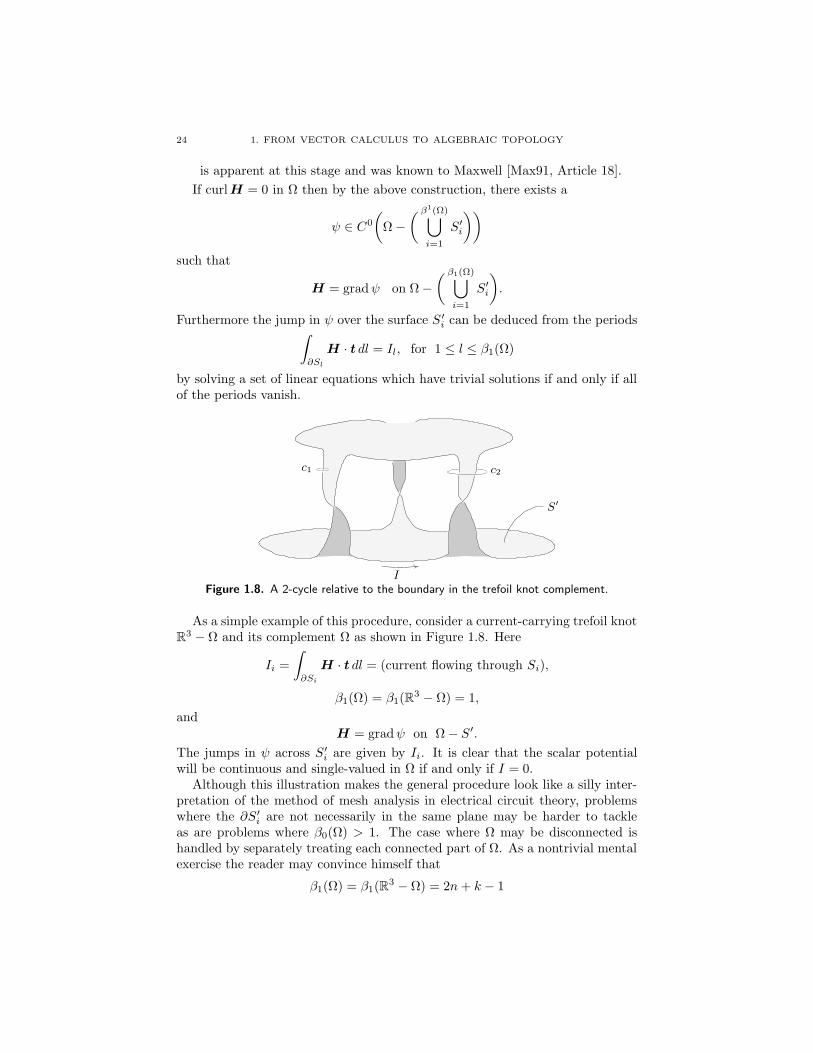
Figure 1.8. A 2-cycle relative to the boundary in the trefoil knot complement.
As a simple example of this procedure, consider a current-carrying trefoil knotR3 −Ω and its complement Ω as shown in Figure 1.8. Here
Ii =
∫
∂Si
H · t dl = (current flowing through Si),
β1(Ω) = β1(R3 − Ω) = 1,
andH = gradψ on Ω− S′.
The jumps in ψ across S′i are given by Ii. It is clear that the scalar potential
will be continuous and single-valued in Ω if and only if I = 0.Although this illustration makes the general procedure look like a silly inter-
pretation of the method of mesh analysis in electrical circuit theory, problemswhere the ∂S′
i are not necessarily in the same plane may be harder to tackleas are problems where β0(Ω) > 1. The case where Ω may be disconnected ishandled by separately treating each connected part of Ω. As a nontrivial mentalexercise the reader may convince himself that
β1(Ω) = β1(R3 −Ω) = 2n+ k − 1

1E. HOMOTOPY VERSUS HOMOLOGY AND LINKING NUMBERS 25
when Ω is the two-dimensional region of example 1.5. This is straightforwardwhen one realizes that generators of H1(Ω) can be taken to be the boundaries ofcuts in R3−Ω and generators of H1(R
3−Ω) can be considered to be boundariesof surfaces which intersect Ω along the cuts ci, where 1 ≤ i ≤ β1(Ω). ˜
1E. Homotopy Versus Homology and Linking Numbers
By some divine justice the homotopy groups of a finite polyhedron or amanifold seem as difficult to compute as they are easy to define.
Raoul Bott [BT82]
While there can be no single-valued scalar potential if the region Ω is notsimply connected, it is not true that the cuts must render the region simplyconnected. One such example has already surfaced in Figure 1.8 where therelative 2-cycle S is a cut for a scalar potential in the scalar potential. Authorsin various fields, including Maxwell [Max91] and others [Str41, Lam32, VB89,AL65, HS85], have assumed that the cut must make the (nonconducting) regionsimply connected. Seeking simple connectivity has led to formulations based onthe notion of homotopy. For two-dimensional problems, the assumption leadsto the right cuts. The relation between homotopy and homology reveals that inthree-dimensional problems such an assumption is not equivalent to the physicalconclusion drawn from Ampere’s law that the problem of making cuts is one oflinking zero current.
While the present objective is to avoid homotopy notions, we briefly considera geometric and algebraic summary of the first homotopy group. The first ho-motopy group π1 of a region V embedded in R3 is an algebraic classificationof all closed loops in V which are topologically different in the sense of contin-uous deformation described below. In order to illustrate homotopy and makethe above description more precise, consider a closed, oriented curve such as thecurrent-carrying trefoil knot shown in Figure 1.9, where V denotes the regioncomplementary to the knot and R3 − V is the knot itself. An arbitrary point pin V is chosen as a base for drawing oriented, closed paths a, b, c, . . . in V . Theset of all closed curves based at p can be partitioned into equivalence classescalled homotopy classes where two closed paths are homotopic if either curvecan be continuously deformed into the other. The path a represents or gener-ates a class [a] which contains all paths homotopic to a. It can be shown thatcomposition of paths induces a product law for homotopy classes, [a][b] = [ab]where we think of ab as traversing a followed by b as shown in Figure 1.9. Theloop a−1 is a with opposite orientation and generates its own homotopy class[a−1] while the constant, or identity, loop e is a path which can be contracted tothe basepoint without encountering the knot. These notions are discussed andextensively illustrated in [Neu79].
It can also be shown that homotopy classes satisfy the following properties:
([a][b])[c] = [a]([b][c]) (associativity),[a][e] = [a] = [e][a] (identity),[a][a−1] = [e] = [a−1][a] (inverse).

26 1. FROM VECTOR CALCULUS TO ALGEBRAIC TOPOLOGY
e
b
bff
c
d
a
Figure 1.9. Closed loops based at p in the region complementary to the cur-rent-carrying knot. Loops a and b are homotopic. So are c and d. Loop e istrivial since it can be contracted to p. Product bf is shown.
Hence, the set of all homotopy classes in V forms a group, written π1, where thegroup law is written as a multiplication. Note that a region is said to be simplyconnected if all loops in the region are homotopic to the identity, in which caseπ1 is trivial. Formally, a multiply connected region is one which is not simplyconnected in this sense.
Particularly significant to π1 are the homotopy classes of the form [xyx−1y−1],called commutators. If π1 is commutative, commutators are equal to the identity,that is xy is deformable to yx so that both represent the same homotopy class,[x][y] = [y][x]. In general π1 is not commutative so that commutators are notequal to the identity and π1 has a commutator subgroup [π1, π1] generated byall possible commutator products.
z1 z3
z2
Figure 1.10.
Example 1.10 Fundamental group of the torus. In reference to Figure 1.10we note that on the torus π1 is generated by z1 and z3, before adding the punctureshown enclosed by z2. In this case the commutator subgroup is trivial so that π1
is commutative. On the other hand, π1 of the punctured torus has a nontrivialcommutator subgroup since the commutator is homotopic to the boundary of

1E. HOMOTOPY VERSUS HOMOLOGY AND LINKING NUMBERS 27
c
I
V
Figure 1.11. c is in the commutator subgroup of π1 for the trefoil knot complementV . c links zero net current and is the boundary of a surface (a disc with a handle)in V .
the hole. Note that in homology, the effect of puncturing the torus becomesapparent only in the second homology group. ˜
The formal relationship between the first homotopy and homology groups isa homomorphism, π1(V ) → H1(V ). The Poincare isomorphism theorem statesthat the kernel of the homomorphism is [π1, π1] so that there is an isomorphism
π1/[π1, π1] ' H1
for any region V . When [π1, π1] is nontrivial, commutators are nontrivial closedloops which, by virtue of the Poincare isomorphism, are zero-homologous. It canbe shown that this is the case [Sti93, GH81], thus commutators are boundariesof surfaces which lie entirely in V . The homology classes of 2-chains bounded byzero-homologous paths can be represented by orientable manifolds in V [Sti93].Hence no current can be linked by a commutator and surfaces bounded by com-mutators are unrelated to surfaces used in Ampere’s law. A proof of the π1-H1
relation can be found in [GH81] and is discussed in the context of Riemann sur-faces and complex analysis in [Spr57]. A discussion of the consequences of theπ1-H1 relation for computational methods can be found in [Cro78].
Figure 1.11 illustrates a commutator element and the surface bounded bythe commutator for the current-carrying trefoil knot where c denotes a class in[π1, π1]. Since c ∈ [π1, π1] and [π1, π1] is the kernel of the Poincare map, c iszero-homologous meaning that a surface S such that c = ∂S exists. By Ampere’sLaw we then have ∫
c
H · dr =
∫
S
J · n ds = 0,
because S lies in V and J = 0 in V . It follows that Link(c, c′) = 0 for c ∈ [π1, π1]and c′ ∈ H1(R
3 − V ).To make the nonconducting region simply connected requires elimination of
all nontrivial closed paths in the region. In problems where [π1, π1] is nontrivial,there exist commutator loops which are zero-homologous, but since commutatorslink zero current, they are unimportant in light of Ampere’s law; and they areirrelevant to finding cuts which make the scalar potential single-valued.

28 1. FROM VECTOR CALCULUS TO ALGEBRAIC TOPOLOGY
The quote at the beginning of this section suggests that there exist other fun-damental problems with a homotopy approach to cuts. While π1 is appealingbecause it “accurately” describes holes in a multiply connected region, practi-cal aspects of its computation continue to be open problems in mathematics[DR91, Sti93]. While π1 is computable for the torus, it is difficult in general toresolve basic decision problems involving noncommutative groups. In homology,groups are abelian and can be expressed as matrices with integer entries. Fur-thermore, for the constructions presented in this book, the matrices associatedwith homology are sparse with O(n) nonzero entries (where n is the number oftetrahedra in the tetrahedralization of a three-dimensional domain) and can becomputed with graph-theoretical techniques. This is made clear in [BS90] and[Rot71] for electrical circuits and is discussed in Chapter 6.
1F. Chain and Cochain Complexes
Chain and cochain complexes are the setting for homology theory. Alge-braically speaking, a chain complex C∗ = Cp, ∂p is a sequence of modules Ciover a ring R and a sequence of homomorphisms
∂p : Cp → Cp−1
such that
∂p−1∂p = 0.
For our purpose, the ring R will be R or Z in which case the modules Cpare vector spaces or abelian groups respectively. A familiar example is the chaincomplex
C∗(Ω; R) = Cp(Ω; R), ∂pconsidered up to now. Similarly, one has the chain complex
C∗(Ω; Z) = Cp(Ω; Z), ∂pwhen the coefficient group is Z.
Cochain complexes are defined in a way similar to chain complexes exceptthat the arrows are reversed. That is, a cochain complex C∗ = Cp, dp is asequence of modules Cp and homomorphisms
dp : Cp → Cp+1
such that
dp+1dp = 0.
An example of a cochain complex is
C∗(Ω; R) = Cp(Ω; R), dpwhich has been considered in the context of integration. When the coefficientgroup is not mentioned, it is understood to be R.
From the definition of chain and cochain complexes, homology and cohomol-ogy are defined as follows. For homology,
Bp = im ∂p+1 and Zp = ker ∂p,

1F. CHAIN AND COCHAIN COMPLEXES 29
so that
Bp ⊂ Zp and Hp = Zp/Bp,
where
βp = RankHp.
For cohomology,
Bp = im dp−1 and Zp = ker dp,
so that
Bp ⊂ Zp and Hp = Zp/Bp,
where
βp = RankHp.
When dealing with chain and cochain complexes, it is often convenient tosuppress the subscript on ∂p and the superscript on dp and let ∂ and d be theboundary and coboundary operators in the complex where their interpretationis clear form context.
The reader should realize that the introduction has thus far aimed to moti-vate the idea of chain and cochain complexes and the resulting homology andcohomology. Explicit methods for setting up complexes and computing homol-ogy from triangulations or cell decompositions can be found in [Mas80, Gib81,Wal57, GH81], while computer programs to compute Betti numbers and othertopological invariants have existed for over four decades [Pin66]. In contrast tothe vast amount of literature on homology theory, there seems to be no systematicexposition on its role in boundary value problems of electromagnetics, thoughearly papers by Bossavit [Bos81, Bos82], Bossavit and Verite [BV82, BV83], Mi-lani and Negro [MN82], Brown [Bro84], Nedelec [Ned78], and Post [Pos78, Pos84]were valuable first steps.
Just as groups, fields and vector spaces are examples of algebraic structures,complexes are a type of algebraic structure and as such it is useful to considermappings between complexes. In the case of a chain complex the useful mappingsto consider are the ones which have nice properties when it comes to homology.Such mappings, called chain homomorphisms, are defined as follows. Given twocomplexes
C∗ = Cp, ∂p and C ′∗ = C ′
p, ∂′p
a chain homomorphism
f∗ : C∗ → C ′∗
is a sequence of homomorphisms fp such that
fp : Cp → C ′p
and
∂′pfp = fp−1∂p.

30 1. FROM VECTOR CALCULUS TO ALGEBRAIC TOPOLOGY
That is, for each p, the diagram
Cp?
fp - C ′p
?
Cp−1
∂p
?fp−1- C ′
p−1
∂′
p
?
? ?
is commutative. In the case of cochain complexes, cochain homomorphisms aredefined analogously.
In order to illustrate chain and cochain homomorphisms, consider a regionΩ and a closed and bounded subset S. Since Cp(S) ⊂ Cp(Ω) for all p and theboundary operator ∂′ in the complex C∗(S) is the restriction of the boundaryoperator ∂ in C∗(Ω) to C∗(S), where C∗(S) is a subcomplex of C∗(Ω). There isa chain homomorphism
i∗ : C∗(S)→ C∗(Ω),
where
ip : Cp(S)→ Cp(Ω)
is an inclusion. Obviously ip−1∂′pc = ∂pipc for all c ∈ Cp(S) as required. Simi-
larly, considering the restriction of a p-form on Ω to one on S for all values of p,there is a cochain homomorphism
r∗ : C∗(Ω)→ C∗(S)
where
rp : Cp(Ω)→ Cp(S).
If the coboundary operator (exterior derivative) in C∗(Ω) is d and the corre-sponding coboundary operator in C∗(S) is d′ then
d′prpω = rp−1dpω for all ω ∈ Cp(Ω)
as required.
Chain Complexes in Electrical Circuit Theory. The notion of a complexis a fundamental idea in electrical circuit theory. Let A be the incidence matrixof branches with vertices, and B the loop matrix of a network. Since ABT = 0there is a chain complex
0→ meshes BT
−→ branches A−→ nodes → 0
in which 2-chains are linear combinations of mesh currents and 1-chains are linearcombinations of branch currents. In addition, the transpose of this complex,results in a cochain complex. Since BAT = 0, there is a cochain complex
0← meshes B←− branches AT
←− nodes ← 0

1F. CHAIN AND COCHAIN COMPLEXES 31
where 0-cochains are linear combinations of potentials at nodes of the network,and 1-cochains are linear combinations of branch voltages [BB69, Sect. 2.2].Furthermore, if the network is planar and A is the reduced incidence matrixobtained by ignoring one node on each connected component of the networkgraph, then the homology of the complex is trivial. Kirchhoff’s laws can beexpressed as
Kirchhoff Voltage Law: v ∈ imAT (or v is a 1-coboundary)
Kirchhoff Current Law: i ∈ kerA (or i is a 1-cycle)
so that if v = AT e for some set of nodal potentials e, then Tellegen’s Theoremis easily deduced:
0 = (e,Ai) = (AT e, i) = (v, i).
Thus Tellegen’s Theorem is an example of orthogonality between cycles andcoboundaries. This view of electrical network theory is usually attributed toWeyl [Wey23] (see also [Sle68, Fla89, Sma72]). Systematic use of homologytheory in electrical network theory can be found in [Chi68] and in the workof Roth [Rot55b, Rot55a, Rot59, Rot71]. Kron [Kro59] generalized electricalnetwork theory by introducing branch relations associated with k-dimensionalones. An explanation of Kron’s method as well as references to additional papersby Kron can be found in [BLG70].
The interplay between continuum and network models through the use ofcomplexes is developed in [Bra66, Ton77, KI59, MIK59]. Examples of cochaincomplexes for differential operators encountered in the work of Tonti and Braninare, for vector analysis in three dimensions where informally, the complex is
0→
scalar
functions
grad−→
field
vectors
curl−→
flux
vectors
div−→
volume
densities
→ 0
with
curl(grad) = 0
div(curl) = 0.
Similarly, in two dimensions,
0→
scalar
functions
grad−→
field
vectors
curl−→ densities → 0.
The two complexes above are special cases of the complex C∗(Ω) considered thusfar; however, when there is no mention of the domain Ω over which functionsare to be defined, it is impossible to say anything about the homology of thecomplex. Hence, unless an explicit dependence on the domain Ω is recognized inthe definition of the complex, it is virtually impossible to say anything concreteabout global aspects of solvability conditions, gauge transformations or comple-mentary variational principles, since these aspects depend on the cohomologygroups of the complex which in turn depend on the topology of the domain Ω.Furthermore, imposing boundary conditions on some subset S ⊂ ∂Ω necessitatesthe consideration of relative cohomology groups to resolve questions of solvabil-ity and gauge ambiguity. Again the situation becomes hopelessly complicated

32 1. FROM VECTOR CALCULUS TO ALGEBRAIC TOPOLOGY
unless a complex which depends explicitly on Ω and S is defined. The cohomol-ogy groups of this complex, which are called the relative cohomology groups ofΩ modulo S are the ones required to describe the global aspects of the givenproblem. Relative homology and cohomology groups are considered in the nextsection.
1G. Relative Homology Groups
Relative chain, cycle, boundary and homology groups of a region Ω modulo asubset S will now be considered. Relative homology groups are the generaliza-tion of ordinary homology groups necessary in order to describe the topologicalaspects of cochains (forms) subject to boundary conditions.
Consider a region Ω and the chain complex C∗(Ω) = Cp(Ω), ∂p associatedwith it. Let S be a compact subset of Ω and C∗(S) = Cp(S), ∂′p be the chaincomplex associated with S. The boundary operator of C∗(S) is the boundaryoperator on C∗(Ω) with a restricted domain. Furthermore,
Cp(S) ⊂ Cp(Ω) for all p.
It is useful to define the quotient group of p-chains on Ω modulo S
Cp(Ω, S) = Cp(Ω)/Cp(S)
when one wants to consider p-chains on Ω while disregarding what happens onsome subset S. In this way, the elements of Cp(Ω, S) are cosets of the form
c+ Cp(S), where c ∈ Cp(Ω).
Although this definition makes sense with any coefficient ring R, in the caseof coefficients in R the definition of Cp(Ω, S) is made intuitive if one definesCp(Ω, S) to be the subset of Cp(Ω) where the support of ω ∈ Cp(Ω, S) lies inΩ − S. In this case it is possible to salvage the idea that integration should bea bilinear pairing between Cp(Ω, S) and Cp(Ω, S). That is,
∫: Cp(Ω, S)× Cp(Ω, S)→ R
should be such that∫
c
ω = 0 for all ω ∈ Cp(Ω, S) implies c ∈ Cp(S)
and ∫
c
ω = 0 for all c ∈ Cp(Ω, S) implies ω = 0.
Note that when S is the empty set, the definitions of relative chain and cochaingroups reduce to those of their absolute counterparts.
Returning to the general case where the chains could be considered withcoefficients in rings such as R or Z, the induced boundary operator
∂′′p : Cp(Ω)/Cp(S)→ Cp−1(Ω)/Cp−1(S)
makes the following definitions appropriate:
Zp(Ω, S) = ker(Cp(Ω, S)
∂′′
p−→ Cp−1(Ω, S))

1G. RELATIVE HOMOLOGY GROUPS 33
is the group of relative p-cycles of Ω modulo S, and
Bp(Ω, S) = im(Cp+1(Ω, S)
∂′′
p+1−→ Cp(Ω, S))
is the group of relative p-boundaries of Ω modulo S. Intuitively, relative cyclesand boundaries can be interpreted as follows. Given z, b ∈ Cp(Ω),
z + Cp(S) ∈ Zp(Ω, S) if ∂pz ∈ ip−1 (Cp−1(S)) ,
b+ Cp(S) ∈ Bp(Ω, S) if ∂p+1c− b ∈ ip (Cp(S)) ,
for some c ∈ Cp+1(Ω). Hence, z is a relative p-cycle if its boundary lies in thesubset S while b is a relative p-boundary if it is homologous to some p-chainon S.
From the definition of ∂ ′′p , it is apparent that
∂′′p ∂′′p+1 = 0.
HenceBp(Ω, S) ⊂ Zp(Ω, S);
the pth relative homology group of Ω modulo S is defined as
Hp(Ω, S) = Zp(Ω, S)/Bp(Ω, S)
and the relative pth Betti number of Ω modulo S as
βp(Ω, S) = RankHp(Ω, S).
By defining Cp(Ω, S) = 0 for p < 0 and p > n, the above definitions make itapparent that
C∗(Ω, S) =Cp(Ω, S), ∂′′p
is a complex. Furthermore, if
jp : Cp(Ω)→ Cp(Ω, S)
is the homomorphism which takes a c ∈ Cp(Ω) into a coset of Cp(Ω, S) accordingto the rule
jp(c) = c+ Cp(S),
then the collection of homomorphisms j∗ = jp is a chain homomorphism
j∗ : C∗(Ω)→ C∗(Ω, S),
since∂′′p jp(c) = jp−1∂p(c) for all c ∈ Cp(Ω).
Though the definitions leading to relative homology groups seem formidable atfirst sight, they are actually quite a bit of fun as the following example shows.
Example 1.11 Two-dimensional example of relative homology. Inthis example the relative homology groups associated with the cross-section ofa coaxial cable are considered. The usefulness of relative homology groups willbecome apparent in later sections once relative cohomology groups have beenintroduced. Consider a piece of coaxial cable of elliptic cross-section, let Ω be the“insulator” as shown in Figure 1.12, and consider 1-chains z, z ′, z′′ and 2-chainsc, c′ as shown in Figure 1.12. From the picture we see that z, z ′, z′′ representnontrivial cosets in Z1(Ω, ∂Ω) but

34 1. FROM VECTOR CALCULUS TO ALGEBRAIC TOPOLOGY
c z
z′′
c′
z′
Figure 1.12. Cycles and relative cycles on elliptical annulus.
j1(z) ∼ 0 in H1(Ω, ∂Ω) since ∂c− z ∈ i1 (C1(∂Ω)) ,
and
j1(z′) ∼ j1(z′′) in H1(Ω, ∂Ω) since ∂c′ − z′ + z′′ ∈ i1 (C1(∂Ω)) .
However, it is apparent that j1(z′) is not homologous to zero in H1(Ω, ∂Ω) and
that β1(Ω, ∂Ω) = 1 so that the cosets of H1(Ω, ∂Ω) are az′+B1(Ω, ∂Ω) for a ∈ R.Next consider the other relative homology groups. Obviously β0(Ω, ∂Ω) = 0,
since any point in Ω can be joined to the boundary by a curve which lies in Ω.Furthermore, considering Ω as a 2-chain in C2(Ω, ∂Ω) it is apparent that
Ω ∈ Z2(Ω, ∂Ω) since ∂2(Ω) ∈ i1 (C1(∂Ω))
hence, since B2(Ω, ∂Ω) = 0, Ω is a nontrivial generator of H2(Ω, ∂Ω) and sincethe region is planar, it is plausible that there are no other independent generatorsof H2(Ω, ∂Ω). Thus β2(Ω, ∂Ω) and the cosets of H2(Ω, ∂Ω) are aΩ for a ∈ R.
In the light of the previous examples the absolute homology groups of theregion Ω are obvious once one notices that β0(Ω) = 1, the 1-cycle z is theonly independent generator of H1(Ω) hence β1(Ω) = 1, and β2(Ω) = 0 sinceZ2(Ω) = 0. Hence, in summary,
β0(Ω) = β2(Ω, ∂Ω) = 1,
β1(Ω) = β1(Ω, ∂Ω) = 1,
β2(Ω) = β0(Ω, ∂Ω) = 0.
In order to exercise the newly acquired concepts, suppose that the capacitanceof the cable was to be determined by a direct variational method. In this caseit is convenient to exploit the inherent symmetry to reduce the problem to one-quarter of the annulus. Consider the diagram shown in Figure 1.13. It is apparentthat for a1, a2 ∈ R, the cosets of H1(Ω
′, S1) and H1(Ω′, S2) look like
a1z1 +B1(Ω′, S1) and a2z2 +B1(Ω
′, S2)
respectively, and that
Z2(Ω′, S1) = 0 = Z2(Ω
′, S2).

1G. RELATIVE HOMOLOGY GROUPS 35
S′′
2
Ω′
z2
S′
1
S′′
1z1
S′
2
Figure 1.13. Cycles and relative cycles of elliptical annulus with respect to symmetryof the full annulus. The boundary ∂Ω′ equals S1 + S2, where S1 = S′
1 + S′′
1 andS2 = S′
2 + S′′
2 .
Henceβ0(Ω
′, S1) = 0 = β2(Ω′, S2),
β1(Ω′, S1) = 1 = β1(Ω
′, S2),
β2(Ω′, S1) = 0 = β0(Ω
′, S2). ˜
Let the pth relative homology group of Ω modulo a subset S with coefficientsin Z, be denoted by
Hp(Ω, S; Z).
This is an abelian group by construction. By the structure theorem for finitelygenerated abelian groups (see [Jac74, Theorem 3.13] or [Gib81, Theorem A.26and Corollary A.27]), this relative homology group is isomorphic to the directsum of a free abelian group F on βp(Ω, S) generators and a torsion group Ton τp(Ω, S) generators, where τp(Ω, S) is called the pth torsion number of Ωmodulo S. When homology is computed with coefficients in R one obtains allthe information associated with the free subgroup F and no information aboutthe torsion subgroup T . It turns out that τp(Ω, S) = 0 if Ω is a subset of R3 andS is the empty set. In other words, for subsets of R3 the torsion subgroups ofthe homology groups
Hp(Ω; Z), for 0 ≤ p ≤ 3,
are trivial (see, for example, [Mas80, Ch. 9, Ex. 6.6] for details). The relationshipbetween Hp(Ω, S; R) and Hp(Ω, S; Z) is important since problems in vector anal-ysis are resolved by knowing the structure of Hp(Ω, S; R) while it is convenientto use integer coefficients in numerical computations and determine Hp(Ω, S; Z).When Hp(Ω, S; Z) is found, the absolute homology groups with coefficients in R
are easily deduced and relative homology groups with coefficients in R are de-duced by throwing away torsion information. The following example illustratesa relative homology group with nontrivial torsion subgroup.
Example 1.12 Torsion phenomena in relative homology. Consider aMobius band which is obtained by identifying the sides of a square I2 as shownin Figure 1.14. Let Ω be the Mobius band and S = za + zb be the 1-chain alongthe edge of the band. Regarding S as a set, the homology groups H1(Ω,Z) and

36 1. FROM VECTOR CALCULUS TO ALGEBRAIC TOPOLOGY
za
z1 I2a
z
z2
z2 I2b z1
zb
z
Figure 1.14. Mobius band. Note that I2 = I2a + I2
b and z = z1 + z2.
H1(Ω, S; Z) will be deduced. The cosets of H1(Ω,Z) are az + B1(Ω,Z) witha ∈ Z so that β1(Ω) = 1.
In contrast, the situation is different when the relative homology group isconsidered. Observe that j1(z) is not homologous to zero in H1(Ω, S; Z), that is∂z ∈ C0(S,Z) but there is no c ∈ C2(Ω,Z) such that ∂c− z ∈ C1(S,Z). However,the square I2 from which Ω was obtained has boundary
∂2(I2) = 2z + zb − za;
hence∂2(I
2)− 2z ∈ i1 (C1(S,Z)) ,
orj1(2z) ∼ 0 in H1(Ω, S; Z).
Thus z is an element of the torsion subgroup of the relative homology groupsince it is not homologous to zero, although a multiple of z is zero-homologous.Similarly j1(z) 6∼ 0 in H1(Ω, S,Z) and j1(2z) ∼ 0 in H1(Ω, S,Z). In order to seethis one may imagine the Mobius band to be made out of paper and is cut alongthe 1-cycle z to yield a surface Ω′. The surface Ω′ is orientable and
∂2(Ω′) = 2z − za − zb
or2z − ∂2(Ω
′) ∈ C1(S,Z).
Hence z and z are nontrivial generators of H1(Ω, S,Z). However z ∼ z since,referring back to the picture, it is apparent that
∂2(I2a) = z1 + z + z2 − za = z + z − za,
∂2(I2b ) = z1 − z + z2 + zb = z − z + zb,
so that
z − (−z)− ∂2(I2a) ∈ C1(S; Z) and z − (z)− ∂2(I
2b ) ∈ C1(S; Z).
That is,j1(z) ∼ j1(z) and j1(z) ∼ −j1(z) in H1(Ω, S,Z).
Thus, it is plausible thatH1(Ω, S; Z) ' Z/2

1H. THE LONG EXACT HOMOLOGY SEQUENCE 37
where Z denotes the integers modulo 2. In summary,
β1(Ω, S) = 0, β1(Ω) = 1, τ1(Ω, S) = 1, τ1(Ω) = 0. ˜
Before considering the role of relative homology groups in resolving topologicalproblems of vector analysis it is useful to consider the long exact homologysequence since it is the key to understanding relative homology.
1H. The Long Exact Homology Sequence
In the context of this book, the long exact homology sequence is a result whichenables one to visualize a full set of generators for the homology of a region Ωmodulo a closed subset S in situations where intuition can be trusted only withthe absolute homology groups of Ω and S. To see how the long exact homologysequence comes about, consider the three complexes
C∗(Ω) = Cp(Ω), ∂p,C∗(S) = Cp(S), ∂′p,
C∗(Ω, S) = Cp(Ω, S), ∂′′p ,and the two chain homomorphisms
i∗ = ip, j∗ = jp,
0→ C∗(S)i∗−→ C∗(Ω)
j∗−→ C∗(Ω, S)→ 0
where the inclusion map ip takes a p-chain on S and sends it to a p-chain whichcoincides with it on S and vanishes elsewhere on Ω−S while jp takes a c ∈ Cp(Ω)and sends it into the coset c+Cp(S) in Cp(Ω, S). It is clear that i∗ is injective,j∗ is surjective and that im i∗ = ker j∗. Such a sequence of three complexesand chain homomorphisms i∗, j∗ is an example of a “short exact sequence ofcomplexes”. When written out in full, the sequence is:
0 - Cp+1(S)?
ip+1- Cp+1(Ω)?
jp+1- Cp+1(Ω, S)?
- 0
0 - Cp(S)
∂′
p+1
?ip- Cp(Ω)
∂p+1
?jp- Cp(Ω, S)
∂′′
p+1
?- 0
0 - Cp−1(S)
∂′
p
?ip−1- Cp−1(Ω)
∂p
?jp−1- Cp−1(Ω, S)
∂′′
p
?- 0
∂′
p−1? ∂p−1
? ∂′′
p−1?
It is a fundamental and purely algebraic result (see [Jac80, Vol. II, Sect. 6.3,Theorem 6.1]) that given such a short exact sequence of complexes, there is a long

38 1. FROM VECTOR CALCULUS TO ALGEBRAIC TOPOLOGY
exact sequence in homology. This means that if ıp and p are the homomorphismswhich ip and jp induce on homology, and δp is a map on homology classes whichtakes z ∈ Zp(Ω, S) into z′ ∈ Zp−1(S) according to the rule
(z′ +Bp−1(S)) = (ip−1)−1∂p(jp)
−1 (z +Bp(Ω, S)) ,
then the diagram
0 - Hn(S)ın - · · · - Hp+1(Ω, S) -
δp+1- Hp(S)ıp- Hp(Ω)
p- Hp(Ω, S) -
δp- Hp−1(S)ıp−1- Hp−1(Ω)
p−1- Hp−1(Ω, S)δp−1 -
· · · 0- H0(Ω, S) - 0
satisfies three conditions:
ker ıp = im δp+1, ker p = im ıp, ker δp = im p.
This result is valid for the coefficient groups Z and R. Here we consider the casewhere homology is computed with coefficients in R so that all of the homologygroups are vector spaces. Let
Hp(Ω, S) '(Hp(Ω, S)
ker δp
)⊕ ker δp.
The two summands can be interpreted using the conditions above. The firstsatisfies
Hp(Ω, S)
ker δp' δ−1
p (im δp) ' δ−1p (ker ıp−1)
by the first condition, and the second satisfies
ker δp = im p ' p(Hp(Ω)
ker p
)' p
(Hp(Ω)
ıp (Hp(S))
)
by the second condition. Thus, Hp(Ω, S) can be rewritten as
(1–3) Hp(Ω, S) ' δ−1p (ker ıp−1)⊕ p
(Hp(Ω)
ıp (Hp(S))
).
By this identity it is usually easy to deduce a set of generators of Hp(Ω, S) ifHp(S), Hp(Ω), Hp−1(S), and Hp−1(Ω) are known. The generators for thesegroups can be found by the following three-step procedure:
(1) Find a basis for the vector space Vp defined by
Hp(Ω) = (im ıp)⊕ Vp.
Hence, p(Vp) gives βp(Ω)− dim im ıp generators of Hp(Ω, S).

1H. THE LONG EXACT HOMOLOGY SEQUENCE 39
(2) Find a basis for ker ıp−1 from the basis for Hp−1(S) so that the
dim ker ıp−1
remaining generators of Hp(Ω, S) can be deduced from
δ−1p (ker ıp−1) .
This is done as follows: Let zi be a basis for ker ıp−1 and find a set of zi, for1 ≤ i ≤ dim ker ıp−1, such that
zi = jp(∂p)−1ip−1zi.
(3) Hp(Ω, S) = (j∗pVp)⊕ δ−1p (ker ıp−1), where a basis results from steps 1 and 2.
Furthermore
βp(Ω, S) = βp(Ω)− dim im ıp + dim ker ıp−1.
Although this procedure is algebraic, it enables one to proceed in a systematicway in complicated problems, as illustrated in the following example.
Example 1.13 Embedded surfaces and relative homology. Recallingthe 2-dimensional surface with n “handles” and k “holes” which was consideredin Example 1.5, we will deduce the relative homology groups H1(Ω, ∂Ω) andH2(R
3,Ω).ForH1(Ω, ∂Ω), consider the long exact homology sequence for the pair (Ω, ∂Ω):
0ı2- H2(Ω)
2- H2(Ω, ∂Ω) -
δ2- H1(∂Ω)ı1- H1(Ω)
1- H1(Ω, ∂Ω) -
δ1- H0(∂Ω)ı0- H0(Ω)
0- H0(Ω, ∂Ω) - 0.
Following the three-step procedure for homology generators H1(Ω, ∂Ω) is ob-tained as follows.
(1) im ı1 and V1 are readily seen to be of the form∑k−1
j=1a2n+jz2n+j + B1(Ω)and
∑2nj=1ajzj +B1(Ω), respectively. That is, j1(z2n+j), with 1 ≤ j ≤ k− 1,
are homologous to zero in H1(Ω, ∂Ω), while j1(zj), for 1 ≤ j ≤ 2n, are nothomologous to zero in H1(Ω, ∂Ω).
(2) The kernel ker ı0 is of the form
k−1∑
j=1
aj(pj − pk) +B0(∂Ω),
while the point pk can be used to generateH0(Ω). Thus the curves j1(C2n+j),for 1 ≤ j ≤ k−1, from Example 1.5 can be used as k−1 additional generatorsin H1(Ω, ∂Ω) since
∂c2n+j = pj − pk for 1 ≤ j ≤ k − 1.

40 1. FROM VECTOR CALCULUS TO ALGEBRAIC TOPOLOGY
(3) Looking at the definitions of the cj , for 1 ≤ j ≤ 2n+ k − 1, it is clear that
2n∑
j=1
ajcj +B1(Ω, ∂Ω) = im 1
and2n+k−1∑
j=2n+1
ajcj +B1(Ω, ∂Ω) = δ−11 (ker ı0) .
Thus, the cosets of H1(Ω, ∂Ω) look like
2n+k+1∑
j=1
ajcj +B1(Ω, ∂Ω);
that is to say, the chains along which cuts were made to obtain a simplyconnected surface yield a set of generators for H1(Ω, ∂Ω), and
β1(Ω) = 2n+ k − 1 = β1(Ω, ∂Ω).
For H2(R3,Ω), consider part of the long exact homology sequence for the pair
(R3,Ω):
· · · ı2−→ H2(R3)
2−→ H2(R3,Ω)
δ2−→ H1(Ω)ı1−→ H1(R
3)1−→ · · ·
Given that
Hp(R3) '
R if p = 0,
0 if p 6= 0,
the part of the long exact sequence displayed above reduces to:
02−→ H2(R
3,Ω)δ2−→ H1(Ω)
ı1−→ 0.
Hence δ2 is an isomorphism since the sequence is exact. It is instructive todeduce H2(R
3,Ω) by the three-step procedure for homology generators:
(1) The first step can be ignored, since H2(R3) ' 0 implies that im 2 = 0.
(2) Since H2(R3,Ω) ' H1(Ω) take generators zi of H1(Ω), for 1 ≤ i ≤ β1(Ω),
and consider δ−12 zi. In other words, relative 2-cycles j2(Si) ∈ Z2(R
3,Ω) mustbe found such that
j2(Si) = j2(∂−12 )i1zi for 1 ≤ i ≤ β1(Ω)
can be used to generate a basis vector of H1(R3,Ω). By individually consid-
ering the “handles” and “holes” of Ω, we easily see that such a set can befound for the jth handle and the jth hole, as illustrated in Figure 1.15.
There is nothing to do at this stage. The cosets of H2(R3,Ω) look like
2n+k−1∑
i=0
aiSi +B2(R3,Ω) for ai ∈ R
and
β2(R3,Ω) = 2n+ k − 1 = β1(Ω).

1I. RELATIVE COHOMOLOGY AND VECTOR ANALYSIS 41
jth handlejth hole
z2j−1
S2j−1
z2jS2j
S2n+j
z2n+j
Figure 1.15. Regions bounded by homology generators of handles on the body inFigure 1.4. For the handle 1 ≤ j ≤ n and for hole 1 ≤ j ≤ k − 1.
It is useful to realize that the same arguments hold if Ω is knotted or has severalconnected components with the exception that representatives of generators ofH2(R
3,Ω) may not be homeomorphic to discs. ˜
Instead of considering more examples of relative homology groups, a heuris-tic argument will now be considered in order to illustrate the use of relativehomology groups in vector analysis.
1I. Relative Cohomology and Vector Analysis
Given a region Ω, one can form a vector space Cpc (Ω) by considering linearcombinations of p-cochains (p-forms) which have compact support in Ω. Sincethe coboundary operator (exterior derivative) applied to a p-cochain of compactsupport yields a p+ 1-cochain of compact support, one can define a complex
C∗c (Ω) = Cpc (Ω), dp
and, by virtue of the fact that one has a complex, the cocycle, coboundary,cohomology groups, and Betti numbers can be defined as usual:
Zpc (Ω) = ker(Cpc (Ω)
dp
−→ Cp+1c (Ω)
),
Bpc (Ω) = im(Cp−1c (Ω)
dp−1
−→ Cpc (Ω)),
Hpc (Ω) = Zpc (Ω)/Bpc (Ω),
βpc (Ω) = Rank (Hpc (Ω)) .
In general, if Ω is a compact region then the cohomology of the complexes C∗c (Ω)
and C∗(Ω) are identical. However, if Ω is an open set then the cohomology ofthe set of complexes will in general be different from C∗
c (Ω) since the cochainswith compact support have restrictions on the boundary of the set.
In order to formulate the idea of relative cohomology, let Ω be a compactregion, S a compact subset, and consider the complexes C∗
c (Ω) = Cpc (Ω), dpand C∗
c (S) = Cpc (S), dp . It is understood that the coboundary operator in thelatter complex is the coboundary operator of the first complex except that thedomain is restricted. In the heuristic motivation for relative homology groups itwas mentioned that in order to regard integration as a bilinear pairing between

42 1. FROM VECTOR CALCULUS TO ALGEBRAIC TOPOLOGY
Cp(Ω, S) and Cp(Ω, S), the definition of Cp(Ω, S) makes sense if Cp(Ω, S) istaken to be the set of linear combinations of p-forms whose support lies in Ω−S.In the present case where Ω and S are assumed to be compact, define the set ofrelative p-cochains to be Cpc (Ω− S). The result is a cochain complex
C∗c (Ω− S) = Cpc (Ω− S), dp ,
where it is understood that the coboundary operator is the restriction of thecoboundary operator in C∗
c (Ω). In analogy with the case of homology, considerthe sequence of complexes
0 −→ C∗c (Ω− S)
e∗−→ C∗c (Ω)
r∗−→ C∗c (S) −→ 0
and the cochain homomorphisms
e∗ = ep , r∗ = rp .Here ep takes a p-cochain on Ω−S and extends it by 0 to the rest of Ω, while rp
takes an p-cochain on Ω and gives its restriction to S. Although this sequence ofcomplexes fails to be exact at C∗
c (Ω), (that is im e∗ 6= ker r∗), a limiting argumentshows that there is still a long exact sequence in cohomology (see [Spi79, p. 589,Theorems 12 and 13]). Furthermore, there exist relative de Rham isomorphisms(see Duff [Duf52] for the basic constructions).
Instead of trying to develop the idea that the coboundary operator in the com-plex C∗
c (Ω − S) is adjoint to the boundary operator in the complex C∗(Ω, S),and trying to justify a relative de Rham isomorphism, familiar examples of therelative isomorphism will be considered. These examples will serve to solidifythe notion of relative homology and cohomology groups and relative de Rhamisomorphism so that an intuitive feel can be developed before a more conciseformalism is given in the next chapter. When considering relative chains onC∗c (Ω − S) there are certain boundary conditions which cochains must satisfy
when S is approached from within Ω− S. Although these conditions are trans-parent in the formalism of differential forms, they will be stated often in thefollowing examples, without proof, since in specific instances they are easily de-duced by using the integral form of Maxwell’s Equations.
In these examples, the relative de Rham isomorphism is understood to mean
Hp(Ω, S) ' Hpc (Ω− S) for all p.
Also, two forms ω1, ω2 ∈ Zpc (Ω− S) are said to be cohomologous in the relativesense if
ω1 − ω2 ∈ Bpc (Ω− S).
As usual, this forms an equivalence relation where the condition above is writtenas
ω1 ∼ ω2.
The notion of a relative period is defined as follows. If ω ∈ Zpc (Ω − S) andz ∈ Zp(Ω, S), the integral
∫zω is called the relative period of ω on z; here,
by Stokes’ theorem, it is easily verified that the period depends only on thecohomology and homology classes of ω and z respectively. Thus the relative

1I. RELATIVE COHOMOLOGY AND VECTOR ANALYSIS 43
de Rham theorem should be interpreted as asserting that integration induces anondegenerate bilinear pairing
∫: Hp(Ω, S)×Hp
c (Ω− S)→ R
where the values of this bilinear pairing can be deduced from evaluating theperiods of basis vectors of Hp
c (Ω−S) on basis vectors of Hp(Ω, S). In most casesthese periods have the interpretation of voltages, currents, charges, or fluxes.
One of the virtues of axiomatic homology theory is that one can show thatonce a method of computing homology for a certain category of spaces, such asmanifolds, has been devised, the resulting homology groups are unique up to anisomorphism. Thus, for example, the de Rham isomorphism can be regardedas a consequence of devising a method of computing cohomology with differen-tial forms and simplicial complexes, and showing that both methods satisfy therequirements of the axiomatic theory in the case of differentiable manifolds.
Example 1.14 Electrostatics: Visualizing H1(Ω, S) in 3 dimensions.Consider a compact subset Ω of R3. On the boundary ∂Ω let ∂Ω be a unionS1∪S2, where S1∩S2 has no area. There is a vector field E in Ω with a constrainton S1 such that:
curlE = 0 in Ω,
n×E = 0 on S1.
No constraint is specified on S2. Elements of C1c (Ω−S1) are associated with vec-
tor fields whose components tangential to S1 vanish, hence E can be associatedwith an element of Z1
c (Ω− S1).Considering the long exact homology sequence for the pair (Ω, S1), one has
H1(Ω, S1) = δ−11 (ker i0)⊕ 1
(H1(Ω)
ı1 (H1(S1))
),
where the relevant portion of the long exact homology sequence is
· · · δ2−→ H1(S1)ı1−→ H1(Ω)
1−→ H1(Ω, S1)δ1−→ H0(S1)
ı0−→ H0(Ω) −→ · · ·Let ci, for 1 ≤ i ≤ β1(Ω, S), be a set of curves which are associated with the
generators of H1(Ω, S1). These curves can be arranged into two groups accordingto the three-step procedure on page 38:
(1) There are dim im j1 generators of H1(Ω, S1) which are homologous in theabsolute sense to generators of H1(Ω). These generators can be associatedwith closed curves ci, for 1 ≤ i ≤ dim im ı1.
Thinking of electromagnetism, the period∫
ci
E · t dl = Vi
is equal to the rate of change of magnetic flux which links ci. Although thereis a static problem in Ω, the periods are associated with magnetic circuitsin R3 − Ω. It is usually wise to set these periods equal to zero if possible.

44 1. FROM VECTOR CALCULUS TO ALGEBRAIC TOPOLOGY
(2) There are dim ker ı0 remaining generators of H1(Ω, S1) which can be asso-ciated with simple open curves whose end points lie in distinct points of S1.In other words, if
c(i+dim im 1) for 1 ≤ i ≤ dimker ı0,
is such a set of curves, they can be defined (assuming Ω is connected) sothat
∂c(i+dim im ) = pi − p0,
where p0 is a datum node lying in some connected component of S1 and eachpi lies in some distinct connected component of S1. That is, there is one piin each connected component of S1.
In this case, the electromagnetic interpretation is that the period∫
ci
E · t dl = Vi
is associated with potential differences between connected components of S1.
Now suppose that the periods of E on generators of the first group vanish.In this case, it is seen from the long exact sequence that the period of E van-ishes on all generators of H1(Ω) since the tangential components of E vanishon S1. Hence, E may be expressed as the gradient of a single-valued scalar φ.Furthermore, the scalar is a constant on each connected component of S1. Thatis, E = gradφ in Ω, where φ = φ(pi) on the ith component of S1.
When E is expressed in this form, the periods of E on the generators ofH1(Ω, S1) which lie in the second group are easy to calculate:
V(i+dim im 1) =
∫
c(i+dim im 1)
gradφ · dl = φ(pi)− φ(p0)
since∂c(dim im 1+1) = pi − p0. ˜
Example 1.15 Magnetostatics: Visualizing H2(Ω, S) in 3 dimensions.As in the previous example, let Ω be a compact subset of R3 such that ∂Ω =S1∪S2 where S1∩S2 has no area. Let B be a vector field in Ω so that div B = 0in Ω and B · n = 0 on S1. There is no constraint on B with respect to S2.Elements of C2
c (Ω − S1) can be identified with vector fields whose componentnormal to S1 vanishes, so B can be associated with an element of Z2
c (Ω − S1).We also let Σi, where 1 ≤ i ≤ β2(Ω, S1), be a set of surfaces associated with abasis of H2(Ω, S1).
The long exact homology sequence for the pair (Ω, S1) is
H2(Ω, S1) = δ−12 (ker ı1)⊕ 2
(H2(Ω)
ı2 (H2(S1))
)
where the relevant portion of the long exact homology sequence is
· · · δ3−→ H2(S1)ı2−→ H2(Ω)
2−→ H2(Ω, S1) −→ δ2−→ H1(S1)ı1−→ H1(Ω)
1−→ · · ·Using the three-step procedure from page 38, surfaces Σi can be arranged intotwo groups:

1I. RELATIVE COHOMOLOGY AND VECTOR ANALYSIS 45
(1) There are dim im 2 generators of H2(Ω, S1) which are homologous in theabsolute sense to generators of H2(Ω). Thus let ∂Σi = 0, for 1 ≤ i ≤dim im 2 and associated to these Σi is a basis of im 2 in H2(Ω, S1).
(2) There are dim ker ı1 remaining generators of H2(Ω, S1) whose image underδ2 form in H1(S1) a basis for ker ı1. Hence let
∂Σdim im 2+i = z1 for 1 ≤ i ≤ dim ker ı1
where the zi are associated with ker i1.
Considering the periods of B on the generators of H2(Ω, S1) in the first group,it is clear that if
B = curlA in Ω
then the periods must vanish because
Φi =
∫
Σi
B · n dS =
∫
∂Σi
A · t dl = 0,
since
∂Σi = 0 for 1 ≤ i ≤ dim im 2.
While this is a restriction, it is still natural to formulate the problem in terms ofa vector potential since the nonzero periods of B on the generators of the firstgroup can only be associated with distributions of magnetic monopoles in R3−Ω.Assuming that the periods of B on the generators of the first group vanish, andB is related to a vector potential A, the periods of B on the generators ofH2(Ω, S1) which lie in the second group can easily be expressed in terms of thevector potential:
Φdim im 2+i =
∫
Σ1+dim im 2
B · n dS =
∫
∂Σdim im 2+i
A · t dl =
∫
zi
A · t dl,
since
∂Σdim im 2+i = zi for 1 ≤ i ≤ dim ker ı1.
It is worthwhile to consider how the tangential components of A are to beprescribed on S1 so that B ·n = 0 and the periods of A can be prescribed. Onecannot impose curlA · n = 0 on S1 by forcing n × A = 0 on S1 because thiswould imply
Φdim im 2+i =
∫
zi
A · t dl = 0,
since
zi ∈ C1c (S1).
Instead, as in the analogous case of electrostatics, one has to let
n×A = n× gradψ = curlψ on S1,
where ψ is a multivalued function of the coordinates on S1. Following the rea-soning in Example 1.5, this function can be made single-valued on
S1 −β1(S1,∂S1)⋃
j=i
di,

46 1. FROM VECTOR CALCULUS TO ALGEBRAIC TOPOLOGY
where the di are a set of curves associated with the generators of H1, (S1, ∂S1)and the periods of the multivalued function ψ are given by specifying the jumpsof ψ on dj , denoted by [ψ]dj
, where 1 ≤ j ≤ β1(S1, ∂S1). To see how this isdone, consider the following portion of the long exact homology sequence for thepair (Ω, S1):
· · · −→ H2(Ω)2−→ H2(Ω, S1)
δ2−→ H1(S1)ı1−→ H1(Ω)
1−→ H1(Ω, S1)δ1−→ · · ·
Using the reasoning of the three-step procedure one has
H1(S1) ' (ı1)−1 (ker 1)⊕ δ2
(H2(Ω, S1)
2 (H2(Ω))
).
Thus the generators of H2(S1) can be arranged into two groups where β1(S2)curves zi, for 1 ≤ i ≤ dim im δ2, can be associated with boundaries of generatorsof H2(Ω, S1). In addition, zi+dim im δ2 curves, for 1 ≤ i ≤ dimker 1, which arehomologous in H1(Ω), are associated to a set of generators of im ı1.
One can define an intersection number matrix I whose ijth entry is the num-ber of oriented intersections of curve zi with curve dj . Then, if pj is the periodof gradψ on zj ,
pi =
∫
zi
A · t dl =
∫
zi
gradψ · t dl
=
β1(S1,∂S1)∑
j=1
Iij [ψ]djfor 1 ≤ i ≤ β1(S1),
where pi = Φi+dim im 2 , for 1 ≤ i ≤ dim im δ2, and the remaining pi are pre-scribed arbitrarily. Assuming, as before, that the matrix with entries mij isnonsingular, the above system of linear equations can be inverted to give thejumps in the scalar ψ in terms of the dim im δ2 periods of the vector potentialand dim ker 1 other arbitrary constants. This technique generalizes and simpli-fies that of [MN82]. The assumption that the matrix with entries mij is squareand nonsingular is a consequence of the Lefschetz duality theorem which will beconsidered in the next chapter. ˜
1J. A Remark on the Association of Relative Cohomology Groupswith Perfect Conductors
The introduction of relative cohomology groups in order to describe the elec-tromagnetic field outside of a good conductor follows logically from two assump-tions:
(1) The normal component of the magnetic flux density vector B and the tan-gential components of the electric field intensity vector E, are continuousacross the interface between two media. One of the two media can be aperfect conductor.
(2) The fields E and B vanish inside a perfect conductor.
In practice, we do not derive the exact conditions under which these assumptionshold on a case-by-case basis, but we do have general criteria for deciding whenthese assumptions are valid. The first assumption follows from the assumption

1J. COHOMOLOGY AND PERFECT CONDUCTORS 47
that the electromagnetic field is finite at every point in space and that the lengthscales of interest are large compared to the size of an atom. Otherwise, thenotion of an interface is open to question. The second assumption pertaining tothe vanishing of fields in a perfect conductor is a little more tricky since a precisejustification depends on the notion of a skin depth, denoted by δ. The generalrule of thumb is that the fields inside a conductor are considered to be negligible ifthe local radius of curvature is much larger than δ. This criterion is simple enoughto understand if we are given δ, but there is a hitch. The skin depth dependson the frequency of the excitation and the material properties of the medium.Hence, the criterion applies to the Fourier transform of the electromagnetic fieldwith respect to time. Specifically, for a nonmagnetic medium of conductivity σand a Fourier component of frequency f , we have in MKS units,
δ =1
2π
√σf
107
.
Although this completes the criteria for deciding whether or not a given conduc-tor behaves like a perfect conductor for some excitation, it is useful to give a fewnumbers by way of example. For copper, σ = 5.6× 10⁷ ohms/meter, so
δ =1
2π√
5.6f.
To relate this to engineering applications involving copper wires, consider thefollowing table, which lists operating frequency and skin depth of several familiarelectromagnetic systems:
Application f δ
Power system 60 Hz 9 mmAM radio 1 MHz 67 µmFM radio / PC motherboard 100 MHz 6.7 µmCellular phone / VLSI circuit 2 GHz 1.5 µm
As a rule, if the conductors are much thicker than the frequency-dependentskin depth, we can assume that the tangential electric fields and the normalmagnetic fields are negligible.
The axiomatic method has many advantages over honest work.Bertrand Russell


May one plow with an ox and an ass together? The like of you may writeeverything and prove everything in quaternions, but in the transition periodthe bilingual method may help to explain the more perfect.
James Clerk Maxwell, in a letter to P. G. Tait.
2Quasistatic Electromagnetic Fields
The purpose of this chapter is to articulate the notion of a quasistatic elec-tromagnetic system, and develop the topological aspects of the boundary valueproblems encountered in the analysis of quasistatic systems. The topological ap-proach gives a new perspective on variational formulations which form the basisof finite element analysis.
2A. The Quasistatic Limit Of Maxwell’s Equations
Maxwell’s Equations. Let S be a surface with boundary, V a volume inR3, and note that ∂ denotes the boundary operator. The integral versions ofMaxwell’s equations are as follows:
∫
∂S
E · dl = − d
dt
∫
S
B · dS (Faraday’s Law)(2–1)
∫
∂V ′
B · dS = 0 (Gauss’ Law for magnetic charge)(2–2)
∫
∂S′
H · dl =d
dt
∫
S′
D · dS +
∫
S′
J · dS (Ampere’s Law)(2–3)
∫
∂V
D · dS =
∫
V
ρ dV (Gauss’ Law)(2–4)
where
E = Electric field intensity vector,
B = Magnetic field flux density vector,
H = Magnetic field intensity vector,
D = Electric field flux density vector,
49

50 2. QUASISTATIC ELECTROMAGNETIC FIELDS
and the current and charge sources are described by
J = Electric current flux density vector,
ρ = Electric charge density.
If we let S′ = ∂V in Ampere’s Law (2–3) and remember that ∂∂ = 0, then thefield vector can be eliminated between Ampere’s and Gauss’ law, (2–3) and (2–4)to reveal a statement of charge conservation:
0 =d
dt
∫
V
ρ dV +
∫
∂V
J · dS.
This shows that conservation of charge is implicit in Maxwell’s equations.When the surfaces and volumes S, S ′, V , V ′ are stationary with respect to the
inertial reference frame of the field vectors, one can use the standard theoremsof vector calculus to rewrite Maxwell’s equations as follows:
curlE = −∂B
∂t,(2–5)
div B = 0,(2–6)
curlH =∂D
∂t+ J ,(2–7)
div D = ρ,(2–8)
div J +∂ρ
∂t= 0.(2–9)
Equations (2–5)–(2–8) are the differential versions of Maxwell’s equations. Equa-tion (2–9) is the differential version of the conservation of charge and can beobtained independently by taking the divergence of Equation (2–7) and substi-tuting in (2–9), remembering that div curl = 0.
The differential versions of Maxwell’s equations are much less general thanthe integral laws for three main reasons:
(1) They need to be modified for use in problems involving noninertial referenceframes. Differential forms are an essential tool for this modification.
(2) The differential laws do not contain “global topological” information whichcan be deduced from the integral laws. The machinery of cohomology groupsis the remedy for this problem.
(3) The differential laws assume differentiability of the field vectors with respectto spatial coordinates and time. However, there can be discontinuities infields across medium interfaces, so it is not possible to deduce the properinterface conditions from the differential laws.
In order to get around the third obstacle, we must go back to the integral lawsand derive so-called interface conditions which give relations for the fields acrossmaterial or media interfaces (Figure 2.1). Here we simply state the interface

2A. THE QUASISTATIC LIMIT OF MAXWELL’S EQUATIONS 51
ab
n
Ea (Ha)
Eb (Hb)
Da (Ba)
Db (Bb)
σs(K)
Figure 2.1.
conditions:
n× (Ea −Eb) = 0,(2–10)
n · (Ba −Bb) = 0,(2–11)
n× (Ha −Hb) = K,(2–12)
n · (Da −Db) = σs,(2–13)
where the superscripts refer to limiting values of the field at on the interface whenthe interface is approached from the side of the indicated medium. The sourcevectors do not really exist in nature but rather represent a way of modelingcurrent distribution in the limit of zero skin depth (that is, when ω = 2πf →∞or σ → 0). This approximation will be discussed soon. From a limiting case ofthe integral laws one has a statement of conservation of surface charge:
n · (Ja − Jb) + divS K +
∂σS∂t
= 0,
where divS is the divergence operator in the interface.In summary, one can say that the integral version of Maxwell’s equations is
equivalent to three distinct pieces of information:
(1) the differential version in regions where constitutive laws are continuous,and the field vectors are continuous and have the appropriate degree ofdifferentiability;
(2) interface conditions where constitutive laws are discontinuous;(3) global topological information which is lost when problems are specified on
subsets of Euclidean space—these are the lumped parameters of circuittheory.
Constitutive Laws. In general, Maxwell’s equations are insufficient for de-termining the electromagnetic field since there are six independent equations intwelve unknowns, namely the components of E, B, D, and H. The first stepto closing this gap is to introduce constitutive laws. For stationary media, these

52 2. QUASISTATIC ELECTROMAGNETIC FIELDS
typically take the form
D = ε0E + P ,
B = µ0(H + M)
and, if J is not fixed, but related to E by Ohm’s law,
J = σ(E + Ei).
The new variables are
ε0 = 8.854× 10⁻¹²farad/meter (permittivity of free space),
µ0 = 4π × 10−7henry/meter (permeability of free space),
σ = conductivity,
P = polarization,
M = magnetization,
Ei = external impressed field due to forces of chemical origin.
Generally the functional relationships
P = P (E, r), M = M(H, r)
are assumed, though sometimes it makes sense to have M = M(B, r).There are several ways to characterize media:
(1) Lossless: ∂Pi/∂Ej = ∂Pj/∂Ei, ∂Mi/∂Hj = ∂Mj/∂Hi when referred toCartesian coordinates.
(2) Homogeneous: P = P (E), M = M(H).(3) Isotropic: P = ε0χe(|E|2, r)E, M = χm(|H|2, r)H where χe and χm are
called the electric and magnetic susceptibilities, respectively.(4) Linear: P is a linear function of E, and M is a linear function of H.
Occasionally the constitutive laws are replaced by linear differential operators:
P = ε0
( 2∑
i=0
χidi
dti
)E.
This leads into the topic of dispersion relations in optics and other interestingphenomena which we will sidestep.
Remark on the concept of energy. The condition for lossless media is equiva-lent to saying that the integrals
∫ E1
E0
D(E) · dE,∫ H1
H0
B(H) · dH
are independent of path connecting initial and final states (at each point inphysical space). Often integration by parts or some monotonicity assumptionthen shows that the values of the integrals
we =
∫ D(E1)
D(E0)
E(D) · dD, wm =
∫ B(H1)
B(H0)
H(B) · dB

2A. THE QUASISTATIC LIMIT OF MAXWELL’S EQUATIONS 53
representing “electric and magnetic energy densities” are defined independent ofhow final states are achieved. When this is so, we define total energies by:
We =
∫
V
we dV, Wm =
∫
V
wm dV
so thatdWe
dt=
∫
V
E · ∂D
∂tdV,
dWm
dt=
∫
V
H · ∂B
∂tdV
Parameters Characterizing Linear Isotropic Media. For linear media theconstitutive relations are simply
D = εE (ε = ε0(1 + χe)),
B = µH (µ = µ0(1 + χm)),
J = σE (Ohm’s Law).
It is often necessary to take a Fourier transform with respect to time in whichcase the frequency parameter ω plays an important role in approximations. Thusthe four parameters, ω, σ, µ, ε describe the behavior of the constitutive relationsat each point in space. From the point of view of wave propagation, it is usuallymore convenient to introduce a different set of parameters:
v =1√µε
(wave speed)
η|σ=0 =
õ
ε(wave impedance in lossless media, i.e. σ = 0)
τe =ε
σ(dielectric relaxation time)
δ =
√2
ωσµ(skin depth)
RS =
√ωµ
2σ(surface resistivity)
(Note that c = 1/√ε0µ0 is the speed of light in vacuum.) Although this set of pa-
rameters is unmotivated at this point, their interpretation and role in simplifyingsolutions will become clear when we consider electromagnetic waves.
The Standard Potentials for Maxwell’s Equations. In this section wepresent the familiar potentials for the electromagnetic field as an efficient way toend up with “fewer equations in fewer unknowns.” Recall Maxwell’s equationsin space-time R3 × R:
curlH = J +∂D
∂t,(2–14)
div D = ρ,(2–15)
curlE = −∂B
∂t,(2–16)
div B = 0.(2–17)

54 2. QUASISTATIC ELECTROMAGNETIC FIELDS
It appears that we have eight scalar equations in twelve unknowns, the twelveunknowns being the components of E,B,D, and H. However, constitutive lawsprovide six more equations so that we should think of the above as eight equationsin six unknowns. The standard potentials enable us to solve equations (2–16)and (2–17) explicitly so that we end up with four equations in four unknowns.
Since Equation (2–17) is valid throughout R3 and the second cohomologygroup of R3 is trivial, we have
(2–18) B = curlA
for some vector potential A. Equations (2–16) and (2–18) can be combined togive
curl
(E +
∂A
∂t
)= 0.
Using the fact that this equation is valid throughout R3, one can conclude thatfor a scalar potential φ
E +∂A
∂t= − gradφ
or
(2–19) E = −∂A
∂t− gradφ.
Equations (2–18) and (2–19) express the six vector components of E and B interms of the four components of A and φ. Note that this is the most generalsolution to Equations (2–16) and (2–17). We have neglected to state conditionson the differentiability of A and φ. However it is straightforward to verify thatthe interface conditions associated with equations (2–16) and (2–17), namely
n× (Ea −Eb) = 0, n · (Ba −B
b) = 0,
are satisfied if A and φ are continuous, and we appeal to energy argumentsto show that A and φ are differentiable if the constitutive laws are smooth inspatial variables. Another way of understanding this is by regarding A and φ tobe solutions to the integral forms associated with (2–16) and (2–17).
The substitution of the potentials (2–18) and (2–19) and constitutive lawsrelating D and H to E and B into Equations (2–14) and (2–15) now yieldsfour scalar equations in four unknowns. It turns out that although Maxwell’sequations and constitutive laws specify E and B uniquely, they do not specifyA and φ uniquely. This ambiguity in the potentials is a result of equations(2–14) and (2–15) being dependent and consistent only if the conservation ofcharge is satisfied. Hence, for a physically meaningful prescription of J and ρ,the potentials are nonunique.
The nonuniqueness of the potentials is summarized by gauge transformationswhich will now be described. Suppose one has two sets of potentials (A, φ) and(A′, φ′) related by the “gauge transformation”
A′ = A + gradχ
φ′ = φ− ∂χ
∂t.
(2–20)

2A. THE QUASISTATIC LIMIT OF MAXWELL’S EQUATIONS 55
It is easy to verify that the gauge transformation leaves the field vectors invariant:
B′ = curlA′ = curlA + curl gradχ = B
since curl grad = 0, and
E′ = −∂A
′
∂t− gradφ′ = −∂A
∂t− ∂
∂t(gradχ)− gradφ+ grad
∂χ
∂t
= −∂A
∂t− gradφ = E.
In this way we see that the substitution of equations (2–18) and (2–19) into(2–14) and (2–15) yields three independent scalar equations for three indepen-dent scalar fields. We expect a solution if and only if the sources J and ρ areprescribed in a way consistent with the conservation of charge. The nonunique-ness of A and φ enables us to add additional constraints which have no physicalsignificance but result in mathematical convenience through a process calledgauge-fixing. Gauge-fixing usually consists of imposing an additional constraintin the form of a linear differential operator acting on A and φ. We consider twoexamples describing the Lorentz and Coulomb gauges.
Example 2.1 The Lorentz gauge. Suppose that
(2–21) div A + µ0ε0∂φ
∂t= 0
is imposed on A and φ as an additional constraint. This places a constraint onthe gauge function χ which can be computed as follows:
0 =(div A
′ + µ0ε0∂φ′
∂t
)−(div A + µ0ε0
∂φ
∂t
)
or
0 = div(A′ −A) + µ0ε0∂
∂t(φ′ − φ).
By Equation (2–20) this becomes
0 = div gradχ− µ0ε0∂2χ
∂t2,
so we see that χ must satisfy a homogeneous wave equation. If suitable boundaryand initial conditions are imposed on div and φ, χ would also be constrainedby homogeneous boundary and initial conditions. Furthermore χ = 0 by theuniqueness of solutions to the wave equation. Hence, the Lorentz condition(2–21) enables A and φ to be specified uniquely. ˜
Example 2.2 The Coulomb gauge. Suppose that
(2–22) div A = 0.
Then, proceeding as before, by (2–20) we have
0 = div A′ − div A = div(A′ −A) = div gradχ.
χ is now constrained to be a harmonic function, and suitable boundary conditionson A force χ to be a constant, and we can once more specify A and φ uniquelyby using the Coulomb gauge (2–22). ˜

56 2. QUASISTATIC ELECTROMAGNETIC FIELDS
Wave Equations and Superposition Integrals. As promised, we will writefour scalar wave equations in the components of A and φ by substituting equa-tions (2–18) and (2–19) into (2–14) and (2–15) and appealing to the constitutiverelations. In order to avoid getting bogged down in modeling of material proper-ties, we will assume the simplest constitutive laws, namely linear, homogeneous,isotropic media. This is accomplished by letting
B = µ0H
and
D = εE (ε ≥ ε0),where ε and µ are constant scalars when the vectors are written in terms ofCartesian coordinates. Hence equations (2–18), (2–19), (2–14), and (2–15) give
(2–23) J = curlH − ∂D
∂t= curl
B
µ− ∂
∂t(εE)
= curl
(1
µcurlA
)+
∂
∂t
(ε∂A
∂t
)+
∂
∂t(ε gradφ)
and
ρ = div D = div(εE) = −div
(ε∂A
∂t
)− div(ε gradφ).
That is,
(2–24) − curl curlA− µε∂2A
∂t2− grad
(µε∂φ
∂t
)= −µJ
and
(2–25) div gradφ+∂
∂t(div A) = −ρ
ε.
Although this is the final product, it is possible to do much better. From thediscussion of gauge invariance we know that we have four equations but, assumingthat J and ρ are prescribed in a manner consistent with the conservation ofcharge, only three equations are independent and one is free to impose a gauge-fixing condition for convenience. In the case at hand, the Lorentz gauge (2–21)uncouples A from φ in Cartesian coordinates. Putting (2–21) into (2–24) and(2–25) results in the following uncoupled equations:
(2–26) grad(div A)− curl(curlA)− µε∂2A
∂t2= −µJ
and
(2–27) div(gradφ)− µε∂2φ
∂t2= −ρ
ε.
It is possible to take one more step by delving into the arcana of Cartesiancoordinates. If some vector field C has the form
C =
3∑
i=1
Ciei

2A. THE QUASISTATIC LIMIT OF MAXWELL’S EQUATIONS 57
in terms of the unit coordinate vectors ei, 1 ≤ i ≤ 3, we have the identity
grad div C − curl curlC =3∑
i=1
(div gradCi)ei.
Applying the vector identity to the vector potential A and substituting into(2–26) gives:
(2–28) div gradAi − µε∂2Ai∂t2
= −µJ i (i = 1, 2, 3).
Thus, φ and the Cartesian components of A all satisfy a wave equation of theform
(2–29) div gradψ − 1
v2
∂2ψ
∂t2= f
where (Section 2A)
v =1√µε
< c =1√µ0ε0
= 3× 10⁸ meters/second.
As a historical note, it was Maxwell who made the fundamental discovery thatadding the displacement current term to Ampere’s Law enables one to show thatelectromagnetic disturbances can propagate and that they do so at the speed oflight. Others had computed the value of (ε0µ0)
−1/2 but attached no physicalsignificance to the number. A further comment is that at this stage, the Lorentzgauge seems to work “like magic.” To demystify it and give a forward pointer tothe use of differential forms, we will simply say that the Lorentz gauge makes thefour-component 1-form (A, φ) a coclosed form on Minkowski space and that theCartesian vector identity is a special case of the Weizenbrock identity relatingthe Laplace–Beltrami operator to the curvature tensor and covariant derivatives.
A more pedestrian view of the Lorentz gauge is that equations (2–27) and(2–28) can now be “solved” by appealing to the fundamental solution of equation(2–29). However, before doing so it is useful to reflect on the possibility ofmisinterpreting these equations by contrasting Equations (2–24) and (2–25) with(2–27) and (2–28). Equations (2–24) and (2–25) have a solution only if theconservation of charge is respected in the prescription of J and ρ. When thisis the case, the potentials are not unique but related by gauge transformation(2–20). On the other hand, Equations (2–27) and (2–28) always have a unique,regardless of how J and ρ are prescribed. To reconcile these statements, it ispossible to derive from equations (2–27) and (2–28) the identity
div grad f − 1
µ0ε0
∂2f
∂t2= div J +
∂ρ
∂t
where
f =1
µ0
(div A + µ0ε0
∂φ
∂t
).
Thus, we see that if the conservation of charge is violated in the modeling ofan electromagnetic device, the potentials cannot satisfy the Lorentz gauge and

58 2. QUASISTATIC ELECTROMAGNETIC FIELDS
so Equations (2–27) and (2–28) are no longer equivalent to (2–24) and (2–25)which describe the electromagnetic field.
Quasistatics and Limitations of Superposition Integrals. It is impor-tant to interpret equations (2–27) and (2–28) in the context of quasistatics. Inparticular, the limits of µ and ε tending to zero give two ways to think of thelimiting case of the speed of light c = 1/
√µε becoming infinite. Electrical engi-
neers call these two limits the electroquasistatic and magnetoquasistatic limits,respectively.
Electroquasistatics (EQS). For the moment let’s ignore interface conditionsand constitutive relations and naively set µ = 0 in Equations (2–21), (2–27),and (2–28). This results in the following equations for the potentials:
div gradφ = −ρε,
div gradAi = 0, for i = 1, 2, 3,
div A = 0.
Thus, since a harmonic function vanishing at infinity is zero, we see that A
vanishes. The electric field is described by the gradient of a scalar potentialwhich can be time-varying. The advantage of the EQS approximation is thatit enables us to work with a scalar potential while ignoring the magnetic field,and then determine the magnetic field as a perturbation by letting µ be a smallparameter.
Magnetoquasistatics (MQS). If we now naively set ε = 0 in equations (2–21),(2–27), and (2–28) we see that the irrotational part of the electric field is unde-fined, and that
div gradAi = −µJi for i = 1, 2, 3,
div A = 0.
Here the Lorentz gauge reduces to the Coulomb gauge, and the magnetic fieldcan be computed from a vector potential. The solenoidal part of the electricfield is also deducible from the vector potential even though the irrotational partis undefined. If one reintroduces a small permittivity ε, and specifies a chargedistribution ρ, the electric field can be modeled quite accurately.
To appreciate the limitations of these two extreme quasistatic limits, considerthe “series RLC circuit” usually encountered in a first course on circuits (Fig-ure 2.2). The second-order linear constant-coefficient differential equation whichresults from applying Kirchhoff’s voltage law is a mathematical model of thecircuit. The model is not valid if the electromagnetic field around the actual cir-cuit is not quasistatic. Note that the converse of this statement is not generallytrue. For the circuit to be quasistatic, we require that the wavelengths of elec-tromagnetic radiation at the Fourier components of v(t) with nontrivial energybe large compared to the overall size of the circuit. Note however that even ifthe circuit can be described by quasistatics, it is neither MQS nor EQS sincethe magnetic field surrounding the inductor is not EQS and the electric field inthe capacitor is not MQS. Furthermore, the circuit model can break down at

2A. THE QUASISTATIC LIMIT OF MAXWELL’S EQUATIONS 59
V
R
L
C
Figure 2.2. RLC circuit.
quasistatic frequencies where “parasitic capacitances” between windings in theinductor come into play.
In general engineering practice the aim is to break a quasistatic system intoEQS and MQS subsystems and a quasistatic field analysis is performed on eachof these subsystems. These subsystems (inductors, capacitors, and so on) arethen given black box models where the terminal variables are related to periodsof closed differential forms. Kirchhoff’s laws then tie the topological informationtogether in order to arrive at circuit equations. In this way electromagnetismand topology become the servants of circuit theory.
There is another perspective on quasistatics and engineering methodology. Ifone does not prescribe the current density J , but rather invokes Ohm’s law, thenin a system which is rigid and can’t do any mechanical work there are only threethings that can happen with the energy in the system. It can be
(1) stored in the electric field,(2) stored in the magnetic field, or(3) dissipated as heat.
Hence, in the analysis of quasistatic systems, one identifies subsystems which areEQS, MQS, or characterized by the laws of steady current conduction. In thecase of linear circuits, we end up with capacitors, inductors, and resistors. Toclarify the process of extracting circuit parameters from EQS, MQS, and ohmicsubsystems from the boundary value problems of computational electromagnet-ics, we devote one section of this chapter to each of these topics. The final sectionof the chapter then combines these three aspects of the electromagnetic field intoa variational picture. However, before leaving the general picture of electromag-netics, we consider the fundamental solution for the scalar wave equation andsee how it provides another framework for quasistatics, one which is not compu-tationally useful but reconciles quasistatics with the theory of electromagneticwaves.
We return to Equation (2–29) as a means to investigating equations (2–27)and (2–28). Since we are trying to avoid issues of boundary values, interfaces,and topology in this section, we consider the wave equations in all of R3, and all

60
2.
QU
ASIS
TAT
ICELEC
TR
OM
AG
NET
ICFIE
LD
S
EQS MQS Steady Currents
(n = 3, p = 1) (n = 3, p = 2) 3-d (n = 3, p = 1) 2-d (n = 2, p = 1)
lumped parameterdefined viarelative period
V =∫cE · dl Φ =
∫S
B · n dS V =∫cE · dl V =
∫zE · dl
relative groups[E · dl] ∈ H1(Ω, ∂Ω) [B · dS] ∈ H2(Ω, ∂Ω) [E · dl] ∈ H1(Ω, S2) [E · dl] ∈ H1(Ω, S2)
[c] ∈ H1(Ω, ∂Ω) [S] ∈ H2(Ω, ∂Ω) [c] ∈ H1(Ω, S2) [z] ∈ H1(Ω, S2)
lumped parameterdefined via dualperiod
Q =∫S
D · n dS I =∫cH · dl I =
∫S
J · n dS I =∫c(K × n
′) · dl
dual
groups[D · dS] ∈ H2(Ω) [H · dl] ∈ H1(Ω) [J · dS] ∈ H2(Ω, S1)
[(K × n′) · dl] ∈
H1(Ω, S1)
[S] ∈ H2(Ω) [c] ∈ H1(Ω) [S] ∈ H2(Ω, S1) [c] ∈ H1(Ω, S1)
quadratic formwhich descends tocohomologyclasses (energy)
∫Ω
E ·D dV =∫∂ΩφD ·dS =
∑i ViQi
=∑
i,j CijViVj
∫Ω
H ·B dV =∫∂Ω
(H ×A) · dS =∑i φiIi =
∑i,j LijIiIj
∫E · JdV =∫
φJ · dS =∑
i ViIi =∑i,j ViRijVj
∫Ω
E ·KdS
topologicalobstructions todual formulations(Lefschetz duality)
D = curlC H = gradψ J = curlH K = n′ × gradχ
Table 2.1. Lumped parameters and cohomology groups

2A. THE QUASISTATIC LIMIT OF MAXWELL’S EQUATIONS 61
time. In this case, the solution to Equation (2–29) takes the form
(2–30) ψ(r, t) = −∫
V ′
f(r0, t− |r−r0|
v )
4π|r − r0| dV ′
so that the solutions to (2–27) and (2–28) are:
A(r, t) = −∫
V ′
µJ(r0, t− |r−r0|
v )
4π|r − r0| dV ′,
Φ(r, t) = −∫
V ′
ρ(r0, t− |r−r0|
v )
4πε|r − r0| dV ′.
(2–31)
These solutions to the wave equations are called the retarded potentials, sincethey look like the solutions to the MQS and EQS problems, respectively, but thetime variable in the sources is delayed by the time it takes for an electromagneticdisturbance to travel from the source to the point of observation. These integralformulae for the solutions also yield the correct insights into precise definitionof quasistatics. Fourier transforms of (2–30) with respect to time look like theMQS and EQS integrals with an extra factor of
expi(2πf/v)|r−r0|
in the integrand (where i =√−1). Hence in order to say that a system is
quasistatic we need to define a highest frequency fmax above which we can agreethat the Fourier components of J and ρ have negligible energy and a maximumdistance lmax which is an upper bound on the distance between any observationpoint of interest and any point where the sources are nonzero. In terms of fmax
and lmax, the engineer’s criterion for a system to be quasistatic is
(2–32) f ≤ fmax v
lmax<
v
|r − r0| .
Here, f is any frequency of interest, and a factor of 10 or greater is usuallyused to interpret the middle inequality. Care must be taken in interpreting v.If ε = εrε0 is evaluated at the frequency of interest, then assuming µ = µ0, wehave (section 2A)
v =1√µ0ε
=1√
εr√µ0ε0
=c√εr.
For example, if a computer circuit board has εr ' 9 when evaluated in the rangeof 108 < f < 109, then we have that v is about one-third the speed of light orv = 108 m/s. Another way to understand the inequalities (2–32) is to rephrasethem in terms of wavelengths. That is, if we define
λ =v
f, λmin =
v
fmax,
then, in terms of wavelength, (2–32) becomes
(2–33) λ ≥ λmin lmax ≥ |r − r0|
This inequality makes clear that there is no clearly defined frequency at which ageneric electromagnetic system stops being quasistatic. Thus, a 60 Hertz powergrid extending across a portion of North America, a 100 MHz circuit board

62 2. QUASISTATIC ELECTROMAGNETIC FIELDS
in a computer, and a package for a 1 GHz microprocessor chip are all similarsituations from the point of view of pushing the limits of quasistatic analysis.Furthermore, it is common to have systems which are not easily categorized.For example, the circuitry in a 1.8 GHz cell phone is designed using quasistaticassumptions while the antenna can’t possibly be designed in this framework.
In summary we can state that Equations (2–31) enable us to articulate thevalidity of quasistatic analysis but do not help us analyze or design quasistaticsystems. There are several reasons why (2–31) play a minor role in quasistatics:
(1) The superposition integrals (2–31) are, in a sense, a fortunate accident result-ing from the ability to exploit the symmetries of Euclidean space in Fourieranalysis. There is no analogous closed form solution in the case of inhomo-geneous media or in the interface conditions associated with generic devicegeometries. This is a practical way of saying that (2–31) are derived undervery restrictive assumptions on constitutive laws.
(2) In typical situations, the “sources” J and ρ are not known a priori but ratherare part of the solution. For instance, in the case of Ohm’s law J is a func-tion of E so that, when restricted to a conducting body, Equations (2–31)become integral equations. The solution to these integral equations is sel-dom attempted when the electromagnetic field in a region of space is to bedetermined (as opposed to a single parameter such as antenna impedanceor a scattering parameter), or when there are volumetric currents. For asurvey of quasistatic applications of integral operators in the context of lowfrequency problems, see [Bos98].
(3) As an elaboration on the above point and as an introduction to this chapteras a whole, we should note that the “excitations” of a quasistatic systemare nonlocal and topological in nature. Specifically, excitations come in theforms of voltages, currents, charges, and fluxes, which are periods of closeddifferential forms. Hence, we seek a formulation and language that brings uscloser to these lumped parameters and associated capacitance, inductance,and resistance matrices (i.e. period matrices). This will be accomplished byidentifying EQS and MQS substructures by focusing on the movement be-tween different forms of energy. We shall see that (2–31) provide a frameworkfor defining quasistatics, but the formalism of analytical mechanics gives usthe power to make “simple” models of quasistatic systems.
(4) Although integral equations have their place in computational electromag-netics, and direct solution of differential equations has the limitation of notbeing useful for unbounded domains, there is no need for ideological debates.Computational electromagnetism has a brutally simple way of resolving thesetypes of debates: once a given computational problem is defined, formula-tions and algorithms have been established, and a computer implementationis chosen, one “merely” looks at the accuracy of the computed solution fora given amount of computation and how this ratio scales with problem size.
As we go along, the above considerations will return to us time and timeagain. We will strive for formulations which are useful for nonlinear constitutivelaws and inhomogeneous media, have a clear link between quasistatic fields and

2B. VARIATIONAL PRINCIPLES FOR ELECTROQUASISTATICS 63
the topological constraints which generate them, propose finite element solutionstrategies, and for the more innovative aspects, we will develop techniques toestimate the amount of computational work for a given task so that there is abasis for comparing different methods.
2B. Variational Principles For Electroquasistatics
The Electroquasistatics Problem. The objective of this section is to un-derstand how the three-step procedure for determining homology generators(page 38) comes into calculations involving the EQS coenergy principle. In par-ticular, we will give a basic statement of the EQS problem and draw connectionsto the groups and the 3-step procedure outlined in Chapter 1. Then we willstate the energy and coenergy functionals for electroquasistatics in the case ofa linear constitutive law and see how these connect to Chapter 1. Finally, forthe case of a linear constitutive law, we evaluate the coenergy functional at theextremum and see how the familiar notion of the capacitance matrix comes outof this process.
Consider a compact region Ω which contains no conducting bodies or freecharges. The boundary ∂Ω = S1 ∪ S2 where S1 ∩ S2 has no area and there areconditions
n×E = 0 on S1,
D · n = 0 on S2.
The boundary condition on S1 is associated with an interface to a conductingbody or to a symmetry plane of the geometry while the boundary condition on S2
can be associated with a symmetry plane. The boundary conditions associatedwith S1 and S2 can also arise on ∂Ω if there exists an interface where thereis a sudden change in permittivity across ∂Ω. Figure 2.3 shows S1 and S2 forthe case of a charged loop after the geometry has been reduced by consideringsymmetries.
S1
S1
S2
S2
——S1
Figure 2.3. Geometry of a charged loop in a box after reduction by problem symmetryto an octant.
At this point it is possible to begin to employ the terminology of Chapter 1.Elements of C1
c (Ω − S1) are associated with vector fields whose components
64 2. QUASISTATIC ELECTROMAGNETIC FIELDS
tangent to S1 vanish. For the electric field intensity E, since
curlE = 0 in Ω,
n×E = 0 on S1,
it is possible to associate E with an element of Z1c (Ω−S1). Similarly (and dually),
elements of C2c (Ω − S2) can be identified with vector fields whose component
normal to S2 vanishes. The electric field flux density D, characterized by
div D = 0 in Ω,
D · n = 0 on S2,
can therefore be identified with an element of Z2c (Ω− S2).
Going to the level of homology, it can be stated that the nondegenerate bilinearpairings
∫: H1(Ω, S1)×H1
c (Ω− S1)→ R,
∫: H2(Ω, S2)×H2
c (Ω− S2)→ R,
induced on homology and cohomology classes by integration, are associated withpotential differences and charges respectively. The fact that there are as manyindependent potential differences as there are independent charges suggests that
β1(Ω, S1) = β2(Ω, S2).
This result is discussed in Chapter 3. For now, by considering a few concretesituations the reader can convince himself that the periods of E on generators ofH1(Ω, S1) are associated with prescribed electromotive forces while the periodsof D on the generators of H2(Ω, S2) correspond to charges.
For variational principles where the electric field E is the independent variableand potential differences are prescribed, the variation of the extremal lies in thespace B1
c (Ω−S1). Dually, for variational principles where the electric flux densityD is the independent variable and charges are prescribed, the variation of theextremal occurs in the space B2
c (Ω− S2).The long exact homology sequence is useful for showing the appropriateness
of the variational principles involving scalar potentials and the limited usefulnessof variational principles involving an electric vector potential. When the electricvector potential is used, the long exact homology sequence indicates how toprescribe the tangential components of the vector potential in terms of a scalarfunction defined on S2. Finally, the vector potential is unique up to an elementof Z1
c (Ω− S2) when its tangential components are prescribed on S2.
Introduction of the Metric. It is useful to illustrate how the various spacesassociated with the cochain complexes C∗
c (Ω − S1) and C∗c (Ω − S2) arise in
variational principles. Assume that there is a tensor constitutive relation
D = D(E, r)

2B. VARIATIONAL PRINCIPLES FOR ELECTROQUASISTATICS 65
and an inverse transformation
E = E(D, r)
such that
D (E(D, r), r) = D.
Furthermore, assuming the matrix
∂Di∂Ej
is symmetric positive definite, then
∂Ei∂Dj
is symmetric positive definite.
The Capacitive Coenergy and Energy Principles. With the metric asdescribed above, the principles of stationary capacitive energy and coenergy canbe stated as follows [Mac70, pp. 332–333]. The stationary capacitive coenergyprinciple is
U(E) = infE∈Z1
c (Ω−S1)
∫
Ω
(∫ E
0
D(ξ, r) · dξ)dV
subject to the constraint that on generators of H1(Ω, S1) periods are prescribedas follows
Vi =
∫
ci
E · dl 1 ≤ i ≤ β1(Ω, S1).
The stationary capacitive energy principle is
U ′(D) = infD∈Z2
c (Ω−S2)
∫
Ω
(∫ D
0
D(ξ, r) · dξ)dV
subject to the constraint that on generators of H2(Ω, S2) periods are prescribedas follows
Qi =
∫
Σi
D · dl 1 ≤ i ≤ β1(Ω, S2).
Note that in both of these variational principles the extremal is a relative co-cycle and when the principal conditions are prescribed on the generators of a(co)homology group the variation of the extremal is constrained to be a relativecoboundary. This is readily seen from the identities
Z1c (Ω− S1) ' H1
c (Ω− S1)⊕B1c (Ω− S1),
Z2c (Ω− S2) ' H2
c (Ω− S2)⊕B2c (Ω− S2).
In the case where the constitutive relations are linear, the coenergy and energyprinciples can be used to obtain upper bounds on capacitance and elastancelumped parameters respectively. This is achieved by expressing the minimum

66 2. QUASISTATIC ELECTROMAGNETIC FIELDS
of the functional as a quadratic form in the prescribed periods and making theidentifications
U(E) =1
2
β1(Ω,S1)∑
i,j=1
ViCijVj , U ′(D) =1
2
β2(Ω,S2)∑
i,j=1
QipijQj .
From the upper bound on elastance, a lower bound on capacitance can be ob-tained in the usual way. The estimation of partial capacitance can be obtainedby leaving certain periods free so that their values can be determined as a byproduct of the minimization.
Not only is the above statement of stationary capacitive energy and coenergyprinciples succinct but it also gives a direct correspondence with the lumpedparameter versions of the same principles. The derivation of the correspondingvariational principles in terms of scalar and vector potentials is instructive sinceinsight is gained into why the coenergy principle is naturally formulated in termsof a scalar potential while the formulation of the energy principle in terms of avector potential requires topological constraints on the model in order for theprinciple to be valid. Let the coenergy principle in terms of a scalar potential beconsidered first.
Capacitance Via Direct Variational Methods with the Stationary Ca-pacitive Coenergy Principle. When E = gradφ the coenergy principle canbe restated as follows:
U(gradφ) = infgradφ∈Z1
c (Ω−S1)
∫
Ω
(∫ φ
0
D (grad η, r) · grad(dη)
)dV,
subject to the constraints
V(i+dim im 1) = φ(pi)− φ(p0), 1 ≤ i ≤ dim ker ı0.
Note that for this functional the space of admissible variations is still B1c (Ω−S1),
that is, φ can be varied by any scalar which vanishes on S1.Although the coenergy principle seems to be more natural when expressed in
terms of a scalar potential, the only difference between the two principles is howthey treat magnetic circuits in R3 − Ω. The situation is quite different whenone tries to express the energy principle in terms of a vector potential since,in general, the energy principle cannot be reformulated in terms of the vectorpotential alone.
We now elaborate on this scalar potential form of the coenergy in order toshow how, when evaluated at the extremum, the capacitance matrix is a naturalresult of the variational principle. To begin, we write the coenergy functional asabove:
(2–34) U(gradφ∗) = infgradφ∈Z′
c(Ω−S1)
∫
Ω
∫ φ
0
D(grad η, r) · grad(dη) dV.
It helps to recall the meaning of gradφ ∈ Z1c (Ω−S1). For this we need the long
exact cohomology sequence
· · · ← H1(Ω)1←− H1(Ω, S1)
δ1←− H0(S1)i0←− H0(Ω)← H0(Ω, S1)← · · ·

2B. VARIATIONAL PRINCIPLES FOR ELECTROQUASISTATICS 67
The connecting homomorphism δ1 describes fields for which E = − gradφ, andgradφ× n = 0 on S1 but φ 6= 0 on S1.
In electrostatics, where ∂B/∂t = 0, the periods of∫
E · dl in H1(Ω) vanishso that 1 is trivial. The nontrivial relative periods are then associated with
(δ1)−1
(H0(S1)
(i0)−1(H0(Ω))
).
Let
S1 =
Rank δ1⋃
i=0
S1i
with S1i connected and disjoint from S1j , for i 6= j. If Ω is connected and φ iszero a single connected component S10 of S1 (i.e., one component is “grounded”),then φ ∈ Z1
c (Ω− S1) means that
φ =
0 on S10,
Vi, for 1 ≤ i ≤ Rank δ1, on S1i,
where the Vi are constants.Differentiating the integral in the space of fields, the variation of this func-
tional becomes
U(grad(φ+ δφ))− U(gradφ) =
∫
Ω
D(gradφ, r) · grad δφ dV +O(‖δφ‖2),
where, since the Vi are constants,
(2–35) δφ = 0 on S1i, 0 ≤ i ≤ Rank δ1.
The first variation δU is integrated by parts as follows. Note from the variationof the functional above that
δU =
∫
Ω
D(gradφ, r) · grad(δφ) dV.
Integrating by parts:
(2–36) δU =
∫
∂Ω
δφ D(gradφ, r) · n dS −∫
Ω
δφ div(D(gradφ, r)) dV.
Since δU must vanish for all admissible variations δφ, Equations (2–35) and(2–36) imply that
div(D(gradφ∗, r)) = 0 in Ω,
D(gradφ∗, r) · n = 0 on ∂Ω− S1,
φ∗ = Vi on S1i, 0 ≤ i ≤ Rank δ1,
(2–37)
where the conditions on φ∗ are global constraints. This is the boundary valueproblem for φ∗.
Next, we would like to evaluate the coenergy functional (2–34) at the ex-tremum using (2–37). Note that the relation
∂Di∂Ej
=∂Dj∂Ei

68 2. QUASISTATIC ELECTROMAGNETIC FIELDS
ensures that the line integral in the functional
U(gradφ∗) =
∫
Ω
(∫ φ∗
0
D(grad η, r) · grad(dη)
)dV
is independent of path. This is how φ goes from the function that vanisheseverywhere to φ∗. Now consider a family of functions φ∗
s(r), parametrized by swhich are solutions to the following boundary value problem which, for 0 ≤ s ≤ 1,is a variant of (2–37) and which interpolates between 0 and φ∗.
div(D(gradφ∗s, r)) = 0 in Ω
D(gradφ∗s, r) · n = 0 on ∂Ω− S1
φ∗s = sVi on S1i, 0 ≤ i ≤ Rank δ1.
(2–38)
Substituting φ∗s into (2–37) gives the following functional:
U(gradφ∗s) =
∫
Ω
(∫ 1
0
D(gradφ∗s, r) · grad
(dφ∗sds
)ds
)dV
Interchanging the order of integration, integrating by parts, and using (2–38)gives
U(gradφ∗s)
=
∫ 1
0
(∫
Ω
D(gradφ∗s, r) · grad
(dφ∗sds
)dV
)ds
=
∫ 1
0
(∫
∂Ω
dφ∗sdsD(gradφ∗
s, r) · n dS −∫
Ω
dφ∗sds
div(D(gradφ∗s, r)) dV
)ds,
where the second term in the last expression is 0 because divD(gradφ∗s , r) van-
ishes in Ω. The remaining term can be split:
U(gradφ∗s) =
∫ 1
0
(∫
S1
dφ∗sdsD(gradφ∗
s, r) · n dS
+
∫
∂Ω−S1
dφ∗sdsD(gradφ∗
s , r) · n dS
)ds,
where the second term vanishes because D(gradφ∗s, r) · n = 0. Then
U(gradφ∗s) =
∫ 1
0
(Rank δ1∑
i=1
∫
S1i
dφ∗sdsD(gradφ∗
s , r) · n dS
)ds.
From (2–38), on S1i
dφ∗sds
=d
ds(sVi) = Vi.
which is a constant, so
U(gradφ∗) =
∫ 1
0
(Rank δ1∑
i=1
Vi
∫
S1i
D(gradφ∗s, r) · n dS
)ds.

2B. VARIATIONAL PRINCIPLES FOR ELECTROQUASISTATICS 69
This can be rewritten as
(2–39) U(gradφ∗) =Rank δ1∑
i=1
Vi
∫ 1
0
Qi(s) ds,
where
Qi(s) =
∫
S1i
D(gradφ∗s, r) · n dS.
Having a relatively neat expression for the stationary value of the functional,we turn to the case of a linear isotropic constitutive law and the notion of acapacitance matrix. In this case, the boundary value problem is linear andQi(s) = sQi so that
∫ 1
0
Qi(s) ds = Qi
∫ 1
0
s ds =Qi2
and Equation (2–39) becomes
(2–40) U(gradφ∗) =1
2
Rank δ1∑
i=1
ViQi.
To develop a basic notion of capacitance matrix, we use the linearity of thepresent case. Let ϕi, 1 ≤ i ≤ Rank δ1 be the unique solutions to the boundaryvalue problem
div(ε(r) gradϕi) = 0 in Ω,
(ε(r) gradϕi) · n = 0 on ∂Ω− S1,
ϕi =
1 on S1i,
0 on S1j if j 6= i.
Using the functions defined above, we can express the solution to this linearisotropic version of (2–37) as
φ∗ =Rank δ1∑
j=1
Vjϕj .
Note that ϕi is dimensionless but φ is not.Furthermore, to evaluate (2–40), we note that
Qi =
∫
S1i
(ε(r) gradϕ∗j ) · n dS =
∫
S1i
Rank δ1∑
j=1
Vj(ε(r) gradϕj) · n dS.
This can be written as
Qi =
Rank δ1∑
j=1
VjCij ,
where the Cij are the entries of the capacitance matrix:
Cij =
∫
S1i
(ε(r) gradϕj) · n dS.

70 2. QUASISTATIC ELECTROMAGNETIC FIELDS
Combining the last two equations with (2–40), we finally have
U(gradφ∗) =1
2
Rank δ1∑
i=1
Rank δ1∑
j=1
CijViVj .
That is, the energy of the linear system is a quadratic form in the voltages, andthe coefficients of the capacitance matrix are as given above. Physically, the Cijrepresent the charge on S1i due to a unit potential on S1j and zero potential onS1k when k 6= j. The capacitance matrix is symmetric and positive definite.
2C. Variational Principles For Magnetoquasistatics
The Magnetoquasistatics Problem. In order to make the connection be-tween the long exact sequence in homology and the definition of lumped param-eters in circuit theory, we will now look at boundary value problems involvingthe magnetic field. Consider a connected compact three-dimensional region Ωwhich contains no infinitely permeable or superconducting material, but whoseboundary may contain an interface with an infinitely permeable or supercon-ducting body. The boundary ∂Ω = S1 ∪ S2 where the two parts comprising theboundary are disjoint, that is S1∩S2 has no area. On each part of the boundarylet there be the following boundary conditions:
B · n = 0 on S1,
n×H = 0 on S2.
The boundary condition on S1 is associated with the boundary of a perfect con-ductor, a superconductor, or a symmetry plane. Alternatively, when Ω containsa very permeable body, part of whose boundary coincides with ∂Ω and it isknown that no flux can escape through that part, the boundary condition forS1 is also appropriate. This latter situation occurs if Ω is an ideal magneticcircuit. The boundary condition on S2 is associated with boundaries of infinitelypermeable bodies or symmetry planes.
Assume that no free currents flow in Ω. Since elements of C2c (Ω − S1) can
be identified with vector fields whose component normal to S1 vanishes, themagnetic flux density B can be associated with an element of Z2
c (Ω−S1) because
div B = 0 in Ω,
B · n = 0 on S1.
Similarly, elements of C1c (Ω − S2) can be associated with vector fields whose
components tangent to S2 vanish. Since it is assumed that no free currentscan flow, the magnetic field intensity H can be associated with an element ofZ1c (Ω− S2) because
curlH = 0 in Ω,
n×H = 0 on S2.
The magnetic flux density B is associated with an element of Z2c (Ω− S1) while
the magnetic field intensity H is associated with an element of Z1c (Ω−S2). The

2C. VARIATIONAL PRINCIPLES FOR MAGNETOQUASISTATICS 71
nondegenerate bilinear pairings∫
: H2(Ω, S1)×H2c (Ω− S1)→ R,
∫: H1(Ω, S2)×H1
c (Ω− S2)→ R,
induced on homology and cohomology classes by integration, are associated withfluxes and magnetomotive forces respectively. In particular, these lumped vari-ables can be associated with the generators of relative homology groups in thefollowing sense. Let
Σi, 1 ≤ i ≤ β2(Ω, S1)
is a set of surfaces associated with a basis of H2(Ω, S1) and
ci, 1 ≤ i ≤ β1(Ω, S2)
is a set of curves associated with a basis of H1(Ω, S2). Then the periods of B
on the Σi,
Φi =
∫
Σi
B · n dS, 1 ≤ i ≤ β2(Ω, S1),
are associated with fluxes, and the periods of H on the ci,
Ii =
∫
ci
H · dl, 1 ≤ i ≤ β1(Ω, S2),
are associated with currents in R3 − Ω.For variational principles involving the magnetic flux density B where fluxes
are prescribed, the variation of the extremal lies in the space B2c (Ω− S1). Typ-
ically it is convenient to reformulate such variational principles in terms of avector potential A. When this is done the tangential components of A are pre-scribed on S1 in order to specify fluxes corresponding to generators of H2
c (Ω−S1)and to ensure that the normal component of B vanishes on S1. In such casesthe vector potential which gives the functional its stationary value is unique towithin an element of Z1
c (Ω− S1).Dually, for variational principles where the magnetic field intensity H is the
independent variable and magnetomotive forces are prescribed, the variation ofthe extremal is in the space B1
c (Ω− S2). Though it is not possible in general toreformulate such principles in terms of a continuous single-valued scalar poten-tial, it is possible to find a scalar potential formulation if one introduces suitablebarriers, called cut surfaces, into Ω, prescribing jumps to the scalar potentialas the surfaces are crossed and fixing the scalar potential to be a different fixedconstant on each connected component of S2.
Whether the variational principles are formulated in terms of vector or scalarpotentials, the long exact homology sequence plays a crucial role in understand-ing the topological implications of the formulations. In addition it sheds lighton prescribing boundary conditions for the vector potential formulation.

72 2. QUASISTATIC ELECTROMAGNETIC FIELDS
Introduction of Metric. In order to illustrate the role of cochain complexesin the statement of variational principles, a constitutive relation must be intro-duced. Let
H = H(B, r)
be a a tensor constitutive relation and let
B = B(H , r)
be the inverse transformation satisfying
B (H(B, r), r) = B.
Furthermore, assume that the matrix with entries
∂Hi∂Bj
is symmetric positive definite. Consequently,
∂Bi∂Hj
is symmetric positive definite.
Stationary Inductive Coenergy and Energy Principles. As stated beforefor electroquasistatics, we now write the inductive energy principles. With themetric as stated, the principles of stationary inductive coenergy and energy arethe following (see also [Mac70, pp. 330–332]) The coenergy principle is
T ′(H) = infH∈Z1
c (Ω−S2)
∫
Ω
∫ H
0
B(ξ, r) · dξ dV,
subject to the constraints that prescribe periods of H on generators ofH1(Ω, S2):
Ii =
∫
ci
H · dl, 1 ≤ i ≤ β1(Ω, S2).
The stationary inductive energy principle is
T (B) = infB∈Z2
c (Ω−S1)
∫
Ω
∫ B
0
H(ξ, r) · dξ dV,
subject to the constraints which prescribe periods of B on generators ofH2(Ω, S1)
Φj =
∫
Σi
B · n dS 1 ≤ i ≤ β2(Ω, S1).
As in the case of electroquasistatics, the extremals in both variational prin-ciples are constrained to be relative cocycles. When principal conditions areprescribed on the generators of a (co)homology group, the variation of the ex-tremal is constrained to be a relative coboundary. This is readily seen from theidentities
Z1c (Ω− S2) ' H1
c (Ω− S2)⊕B1c (Ω− S2),
Z2c (Ω− S1) ' H2
c (Ω− S1)⊕B1c (Ω− S1),

2C. VARIATIONAL PRINCIPLES FOR MAGNETOQUASISTATICS 73
and the fact that the following relative de Rham isomorphisms have been as-sumed:
H1c (Ω− S2) ' H1(Ω, S2) H2
c (Ω− S1) ' H2(Ω, S1).
For linear constitutive relations the coenergy principle gives an upper boundfor inductance while the energy principle gives an upper bound for inverse induc-tance. This is done by expressing the minimum of the functional as a quadraticform in the prescribed periods and making the identifications
T ′(H) =1
2
β1(Ω,S2)∑
i,j=1
IiLijIi, T (B) =1
2
β2(Ω,S1)∑
i,j=1
ΦiΓijΦj .
From the upper bound on inverse inductance a lower bound on inductance canbe found in the usual way. The estimation of partial inductances can be obtainedby leaving some of the periods free in a given variational principle so that theirvalues can be determined by the minimization.
These variational principles are interesting since they provide a direct linkwith lumped parameters and show how the various subspaces of the complexesC∗c (Ω−S1) and C∗
c (Ω−S2) play a role. As in the case of electrostatics it is usefulto further investigate the relative (co)homology groups of concern in order to seehow the above variational principles can be rephrased in terms of vector andscalar potentials and to know the topological restrictions which may arise.
The Inductive Energy Principle with a Vector Potential. While we willbriefly state the stationary inductive energy principle in terms of a vector poten-tial, we will not use it for calculations, preferring to concentrate on calculationswith the coenergy principle and scalar potential. The stationary inductive energyprinciple with B = curlA is
T (curlA) = infA
∫
Ω
∫ A
H(curl ξ, r) · curl(dξ) dV,
subject to the principal boundary condition
n×A = curlψ on S1,
where [ψ]djis prescribed on generators of H1(S1, ∂S1) but ψ is otherwise an
arbitrary single-valued function. Note that in this formulation of the energyprinciple the extremal A is unique to within an element of Z1
c (Ω− S1). Since
Z1c (Ω− S1) = H1
c (Ω− S1)⊕B1c (Ω− S1),
the nonuniqueness can be overcome by specifying the periods of A on the gen-erators of H1(Ω, S1) and, in analogy with the uniqueness considerations of theelectric vector potential, specifying the divergence of A and its normal compo-nent on S2 eliminates the ambiguity in B1
c (Ω− S1). More detailed explorationsof topological aspects of the vector potential in magnetostatics occur in Exam-ples 1.15 and 3.4.

74 2. QUASISTATIC ELECTROMAGNETIC FIELDS
The Inductive Coenergy Principle with a Scalar Potential. As in thecase of the capacitive coenergy principle, the three-step procedure from page 38which came about from the long exact homology sequence plays a role in theinductive coenergy principle. The added twist is that in order to formulatethe principle in terms of a scalar potential, cuts must be introduced in orderto make the scalar potential single-valued. The introduction of cuts requiresa certain amount of additional bookkeeping, but the method is essentially thesame as before. There are questions of what cuts are and how they might becomputed. These matters are treated more fully in later chapters.
In terms of a scalar potential, the inductive coenergy functional is
T ′(gradψ) = infgradψ∈Z1
c (Ω−S2)
∫
Ω−
∫ ψ
0
B(ξ, r) · dξ dV,
where Ω− = Ω−∪Σ′i, 1 ≤ i ≤ dim im 1 denotes the region Ω with cuts removed.
Consider the following portion of the long exact homology sequence associatedwith the pair (Ω, S2):
· · · δ2−→ H1(S2)ı1−→ H1(Ω)
1−→ H1(Ω, S2)δ1−→ H0(S2)
ı0−→ H0(Ω)0−→ · · ·
According to the prescription given by Equation (1–3) (page 38), the generatorsof H1(Ω, S2) can be constructed from the three-step procedure for
H1(Ω, S2) ' δ−11 (ker ı0)⊕ 1
(H1(Ω)
ı1 (H1(S2))
).
Let ci, for 1 ≤ i ≤ β1(Ω, S2), be a set of curves which are associated with thegenerators of H1(Ω, S2). The generators can be classified into two groups whichlend some insight into the periods of H.
The first group consists of dim im 1 generators of H1(Ω, S2) which are ho-mologous in the absolute sense to generators of H1(Ω). These generators can beassociated with closed curves ci, 1 ≤ i ≤ dim im 1. In this case, the period
∫
ci
H · dl = Ii
is equal to the current in R3−Ω which links the generator ofH1(Ω, S2) associatedwith ci.
The second group consists of dim ker ı0 remaining generators of H1(Ω, S2)which are associated with simple open curves whose end points lie in distinctconnected components of S2. That is, in each connected component of Ω, onecan find curves ci+dim im 1 , for 1 ≤ i ≤ dim ker ı0, such that
∂ci+dim im 1 = pi − p0,
where p0 is a datum node lying in some connected component of S2 and each pilies in some other distinct connected component of S2. In this case, the period
∫
cj
H · dl = Ij , dim im 1 < j ≤ β1(Ω, S2)
is associated with a magnetomotive force.

2C. VARIATIONAL PRINCIPLES FOR MAGNETOQUASISTATICS 75
It is often convenient to describe the magnetic field intensity H in terms of ascalar potential ψ since, from a practical point of view, it is much easier to workwith a scalar function than three components of a vector field. However, whenthe periods of H do not vanish on the 1-cycles in the first group, then it is notpossible to make ψ continuous and single-valued since this would imply
Ii =
∫
ci
H · dl =
∫
ci
gradψ · dl = 0
since
∂ci = 0, 1 ≤ i ≤ dim im 1.
In order to overcome this difficulty one can perform an analog of the procedureused to prescribe the tangential components of the vector potential. There existcut surfaces
Σ′i, 1 ≤ i ≤ dim im 1,
such that the Σ′i are associated with subspaces of H2(Ω, S1) of dimension equal
to dim im 1. Let Int (ci,Σ′j) denote the number of oriented intersections of the
1-chain ci with the relative 2-chain Σ′j and let I be the the dim im 1×dim im 1
matrix such that
Iij = Int (ci,Σ′j).
The intersection matrix I is nonsingular as will be apparent when duality theo-rems are considered. It turns out that one can make the scalar potential single-valued on
Ω− = Ω−dim im 1⋃
i=1
Σ′i.
Assuming that the Σ′i have been chosen properly, the periods of H on the
generators of H1(Ω, S2) which lie in the first group of generators are easily ex-pressed in terms of the jumps in ψ as the Σ′
i are traversed. That is, if [ψ]Σ′
iare
these jumps, then for 1 ≤ i ≤ dim im 1 one has
Ii =
∫
ci
H · dl =
∫
ci
gradψ · dl =
dim im 1∑
j=1
Iij [ψ]Σ′
j.
This forms a set of linear equations which can be inverted to yield
[ψ]Σ′
i=
dim im 1∑
j=1
I−1ij Ij .
Thus, once the cuts have been selected, one has an explicit way of prescribingthe first dim im 1 periods of H in terms of the jumps in ψ. In order to specifythe remaining dimker ı1 periods of H in terms of the scalar function ψ, onedefines a dim ker ı0 × dim im 1 intersection matrix I ′ij whose entries are the
number of oriented intersections of curves ci+dim im 1 with surfaces Σ′i. Hence

76 2. QUASISTATIC ELECTROMAGNETIC FIELDS
the periods H on the remaining generators can be expressed as follows:
Ii+dim im 1 =
∫
ci+dim im j1
H · dl =
∫
ci+dim im 1
gradψ · dl
= ψ(pi)− ψ(p0) +
dim im j1∑
j=1
I ′ij [ψ]Σ′
j.
Hence, if ψ(p0) is chosen arbitrarily, we have
ψ(pi) = ψ(p0) + Ii+dim im 1 −dim im 1∑
j=1
I ′ij [ψ]Σ′
j
= ψ(p0) + Ii+dim im 1 −dim im 1∑
l,j=1
I ′ij(Ijl)−1Il,
which is an explicit formula giving the value of ψ(pi) in terms of the remainingperiods to be prescribed.
Note that on the ith connected component of S2
ψ = ψ(pi), 0 ≤ i ≤ dim im δ1
since the tangential components of H vanish on S2.
Inductance Parameters from the Inductive Coenergy Principle. Withthe foregoing discussion in mind, we will show the calculations which lead toinductance parameters. Once cuts have been introduced, the calculations are,in almost every respect, parallel to the ones previously done for capacitanceparameters. We start with the inductive coenergy functional
(2–41) T ′(gradψ) = infgradψ∈Z1
c (Ω−S2)
∫
Ω−
∫ ψ
0
B(ξ, r) · dξ dV,
where
Ω− = Ω−⋃
1≤i≤dim im 1
Σ′i
denotes the region Ω with cuts removed. The functional is subject to the follow-ing constraints:
[ψ]Σ′
i6= 0 on cuts Σ′
i, 1 ≤ i ≤ dim im 1,
n · B(gradψ, r) = 0 on S1,
n× gradψ = 0 on S2,
ψ = ψ(pi) on S2i.
The last constraint specifies a given constant on each connected component ofS2. In particular, for the last constraint let
S2 =
Rank ker ı0−1⋃
i=0
S2i,

2C. VARIATIONAL PRINCIPLES FOR MAGNETOQUASISTATICS 77
with S2i connected and disjoint from S2j when i 6= j. If Ω is connected and ψ iszero on S20 (i.e., one component is grounded), then ψ ∈ Z1
c (Ω− S2) means that
ψ =
0, on S20,
ψ(pi), 1 ≤ i ≤ Rank ker ı0 − 1) on S2i,
where the ψ(pi) are constants.Differentiating functional (2–41) in the space of fields and taking the variation,
the functional becomes(2–42)
T ′(gradψ + δψ)− T ′(gradψ) =
∫
Ω−
B(gradψ, r) · grad(δψ) dV +O(‖δψ‖2).
Since the ψ(pi) are constants, δψ = 0 on S2i.The first variation of the functional is the part of (2–42) which is linear in
δψ. Taking the first variation and integrating by parts,
δT ′ =
∫
∂Ω−
δψ B(gradψ, r) dS −∫
Ω−
δψ divB(gradψ, r) dV.
Since δT ′ must vanish for all admissible variations of T ′, this equation impliesthat the following boundary value problem is satisfied at the extremum ψ∗:
(2–43)
divB(gradψ∗, r) = 0 in Ω−,
B(gradψ∗, r) · n0 on S1,
ψ∗ = ψ(pi) on S2i,
with [ψ∗]Σ′
iprescribed on Σ′
i for 1 ≤ i ≤ dim im 1.
Recall that the constitutive law satisfies the relation
∂Bi∂Hj
=∂Hj∂Bj
,
so that the line integral in the functional
T ′(gradψ∗) =
∫
Ω−
(∫ ψ∗
0
B(grad η, r) · grad(dη)
)dV
is independent of path. We now take a family of functions ψ∗s (r), parametrized
by s, with 0 ≤ s ≤ 1, which are solutions to the boundary value problem whichis a variant of (2–43) and provides a linear interpolation between 0 and ψ∗.Putting ψ∗
s into the preceding,
T ′(gradψ∗s ) =
∫
Ω−
(∫ 1
0
B(gradψ∗s , r) · grad
(dψ∗
s
ds
)ds
)dV.

78 2. QUASISTATIC ELECTROMAGNETIC FIELDS
Now interchange the order of integration and integrate by parts:
T ′(gradψ∗s )
=
∫ 1
0
(∫
Ω−
B(gradψ∗s , r) · grad
(dψ∗s
ds
)dV
)ds
=
∫ 1
0
(∫
∂Ω−
dψ∗s
dsB(gradψ∗
s , r) · n dS −∫
Ω−
dψ∗s
dsdiv(B(gradψ∗
s , r)) dV
)ds
+
∫ 1
0
( dim im 1∑
i=1
∫
Σ′
i
[∂ψ∗
s
∂s
]
Σ′
i
B (gradψ∗s , r) · n dS
)ds.
The second term in the last expression vanishes because div(B(gradψ∗s , r)) = 0
and the first term can be split so that
T ′(gradψ∗s ) =
∫ 1
0
(∫
S2
dψ∗s
dsB(gradψ∗
s , r) · n dS
+
∫
∂Ω−−S2
dψ∗s
dsB(gradψ∗
s , r) · n dS
)ds
+
∫ 1
0
( dim im 1∑
i=1
∫
Σ′
i
[∂ψ∗
s
∂s
]
Σ′
i
B (gradψ∗s , r) · n dS
)ds,
where the second term vanishes because B(gradψ∗s , r) · n = 0 on S2. Then
T ′(gradψ∗s ) =
∫ 1
0
( dim ker ı0−1∑
i=1
∫
S2i
dψ∗s
dsB(gradψ∗
s , r) · n dS)ds
+
∫ 1
0
( dim im 1∑
i=1
∫
Σ′
i
[∂ψ∗
s
∂s
]
Σ′
i
B (gradψ∗s , r) · n dS
)ds.
Note thatdψ∗
s
ds=
d
ds(sIi) = Ii
is a constant on S2i while a similar relation exists on Σ′i. Hence,
T ′(gradψ∗s ) =
∫ 1
0
( dim ker ı0−1∑
i=1
Ii
∫
S2i
B(gradψ∗s , r) · n dS
)ds
+
∫ 1
0
( dim im 1∑
i=1
∫
Σ′
i
[∂ψ∗
s
∂s
]
Σ′
i
B (gradψ∗s , r) · n dS
)ds.
This can be rewritten as
(2–44) T ′(gradψ∗s ) =
dim ker ı0−1∑
i=1
Ii
∫ 1
0
Φi(s) ds
+
dim im 1∑
i=1
[ψ]Σ′
i
∫ 1
0
(∫
Σ′
i
B(gradψ∗s , r) · n dS
)ds,

2C. VARIATIONAL PRINCIPLES FOR MAGNETOQUASISTATICS 79
where
Φi(s) =
∫
S2i
B(gradψ∗s , r) · n dS,
for 1 ≤ i ≤ dim ker ı0 − 1. On the cuts we have
Φdim ker ı0−1+i =
∫
Σ′
i
B(gradψ∗s , r) · n dS
for dim ker ı0 < i ≤ β1(Ω, S2).Finally, we develop the expression for the energy of a linear system of currents
which comes out of the preceding variational process. This expression comesabout by a calculation similar to the one made for electroquasistatics and con-tains the notion of inductance parameters. We take the case of a linear isotropicconstitutive law so that the boundary value problem is linear and Φi(s) = sΦi.Then ∫ 1
0
Φi(s) ds = Φi
∫ 1
0
s ds =Φi2
and (2–44) becomes
(2–45) T ′(gradψ∗) =1
2
dim ker ı0−1∑
i=1
IiΦi +
dim im 1∑
j=1
[ψ∗]Σ′
jΦdim ker ı0−1+j .
Let ψi, 1 ≤ i ≤ dim ker ı0 − 1 be the unique solutions to the boundary valueproblem
[ψi] = 0 on Σ′k for all k,
div(µ(r) gradψi) = 0 in Ω
(µ(r) gradψi) · n = 0 on ∂Ω− S2
ψi =
1 on S2i,
0 on S2j if j 6= i.
Note that ψi is dimensionless but ψ is not. Similarly, for dim im 1 ≤ i ≤β1(Ω, S2), we let
[ψi]Σ′
j=
1 if i = dim ker ı0 + j,
0 otherwise,
div(µ(r) gradψi) = 0 in Ω,
µ(r) gradψi · n = 0 on ∂Ω− S2,
ψi = 0 on S2k for all k.
Using the functions defined above, we can express the solution to this linearisotropic version of (2–43) as
ψ∗ =
dim ker ı0−1∑
j=1
Ijψj +
dim im 1∑
j=1
[ψ]Σ′
jΦdim ker ı0−1+j .

80 2. QUASISTATIC ELECTROMAGNETIC FIELDS
To evaluate (2–45), note that
Φi =
∫
S2i
(µ(r) gradψ∗) · n dS
=
∫
S2i
dim ker ı0−1∑
j=1
Ij(µ(r) gradψj) · n dS
+
∫
S2i
dim im 1∑
j=1
[ψ]Σ′
j(µ(r) gradψdim ker ı0−1+j) · n dS.
In principle this can be written as
Φi =
β1(Ω,S2)∑
j=1
IjLij ,
where the Lij are the entries of the inductance matrix.This step necessarilyinvolves rewriting the [ψ∗]Σ′
jin terms of exterior currents by means of linking
information. Combining the last equation with (2–45), we have
T ′(gradψ∗) =1
2
β1(Ω,S2)∑
i=1
β1(Ω,S2)∑
i=1
LijIiIj .
The energy of the linear system is a quadratic form in the currents, and thecoefficients of the inductance matrix are as given above. Physically, the entriesof the first block of Lij represent the flux linking surface S2i due to a unit currenton S2j and zero current on S2k when k 6= j. The second block on the diagonalof the inductance matrix relates to the currents circulating on the boundaries ofthe cuts. The inductance matrix is symmetric and positive definite.
2D. Steady Current Flow
We will soon see that in the modeling of quasistatic electromagnetic systemswhere no mechanical work is being performed, it is important to track the electricand magnetic energy, as well as the energy dissipated as heat. Having consideredelectrostatics and magnetostatics in the previous two sections, we now turn tosteady current conduction. This sets the stage for our discussion of electroqua-sistatic modeling in the next section.
Example 2.3 Steady Current conduction in three dimensions: n = 3,p = 2. Consider a connected compact region Ω of finite, nonzero conductivityand whose boundary may contain interfaces with nonconducting or perfectlyconducting bodies. Let ∂Ω = S1 ∪ S2, where S1 ∩ S2 has no area, and suppose
div J = 0 in Ω,
J · n = 0 on S1,
curlE = 0 in Ω,
n×E = 0 on S2.

2D. STEADY CURRENT FLOW 81
It is readily seen that the transformation
J → B, E →H,
makes this problem formally equivalent to example 1.15. It is clear that currentdensity J can be associated with an element of Z2
c (Ω − S1). The electric fieldintensity E can be associated with an element of Z1
c (Ω − S2). Note that theboundary condition on S1 can be associated with a symmetry plane or interfacewith a nonconducting body while the boundary condition on S2 can be associatedwith another type of symmetry plane or the interface of a perfectly conductingbody. If
Σi, 1 ≤ i ≤ β2(Ω, S1),
is a set of surfaces associated with a basis of H2(Ω, S1) then the periods of J onthe Σi,
Ii =
∫
Σi
J · n dS, 1 ≤ i ≤ β2(Ω, S1),
are associated with currents. In addition, if
ci, 1 ≤ i ≤ β1(Ω, S2),
is a set of curves associated with a basis of H1(Ω, S2), then the periods of E onthe ci
Vi =
∫
ci
E · dl, 1 ≤ i ≤ β1(Ω, S2),
are associated with voltages, or electromotive forces.To obtain a variational formulation of the problem, consider a constitutive
relation
E = E(J , r)
and an inverse constitutive relation
J = J (E, r)
which satisfies
E (J (E, r), r) = E.
Furthermore, assume that the two matrices with elements
∂Ei∂Jj
,∂Ji∂Ej
are symmetric and positive definite. In this case the principles of stationarycontent and cocontent can be stated as follows (see [Mac70, pp. 329–330]).
Stationary Content Principle.
G(J) = infJ∈Z2
c (Ω−S1)
∫
Ω
(∫ J
0
E(ξ, r) · dξ)dV,
subject to the constraints which prescribe the periods of J on generators ofH2(Ω, S1)
Ii =
∫
Σi
J · n dS, 1 ≤ i ≤ β2(Ω, S1)

82 2. QUASISTATIC ELECTROMAGNETIC FIELDS
Stationary Cocontent Principle.
G′(E) = infE∈Z1
c (Ω−S2)
∫
Ω
(∫ E
0
J (ξ, r) · dξ)dV
subject to the constraints which prescribe the periods of E on generators ofH1(Ω, S2)
Vi =
∫
ci
E · dl, 1 ≤ i ≤ β1(Ω, S2).
As in the previous two examples, the two variational principles stated aboveconstrain the extremal to be a relative cocycle and when additional constraintsare prescribed on the generators of a (co)homology group, the variation of theextremal is constrained to be a relative coboundary.
For linear constitutive relations the content principle gives an upper boundfor resistance while the cocontent principle gives an upper bound on conduc-tance. As usual the upper bounds are obtained by expressing the minimum ofthe functional as a quadratic form in the prescribed periods and making theidentifications
G(J) =
β2(Ω,S1)∑
i,j=1
IiRijIj , G(E) =
β1(Ω,S2)∑
i,j=1
ViGijVj .
From the upper bound on conductance, a lower bound on resistance can be foundin the usual way.
By attempting to express the variational principles in terms of vector andscalar potentials one will find, as in previous examples, many topological sub-tleties. Noticing the mathematical equivalence between this example involvingsteady currents and the previous one involving magnetostatics, one may form atransformation of variables
J → B, E →H, T → A, φ→ ψ,
as soon as one tries to define potentials φ and T such that
J = curlT , E = gradφ.
Summarizing the results of exploiting the mathematical analogy, one can saythe following about the cocontent principle in terms of a vector potential T . Asin the previous example, one can consider the long exact homology sequence forthe pair (Ω, S1) and obtain
H2(Ω, S1) = δ−12 (ker ı1)⊕ 2
(H2(Ω)
ı2 (H2(S1))
)
where the relevant portion of the long exact homology sequence is
· · · δ3−→ H2(S1)ı2−→ H2(Ω)
2−→ H2(Ω, S1)δ2−→ H1(S1)
ı1−→ H1(Ω)1−→ · · ·
As in the case of the vector potential A in Example 1.15, the surfaces Σi, 1 ≤i ≤ β2(Ω, S1) can be split up into two groups where the first group is associated

2D. STEADY CURRENT FLOW 83
with a basis of the second term in the direct sum and the periods vanish on thisfirst group. That is: the set
Σi, 1 ≤ i ≤ dim im 2,
is related to a basis for im 2 and
Ii =
∫
Σi
J · n dS =
∫
∂Σi
T · dl = 0
since
∂Σi = 0, 1 ≤ i ≤ dim im 2.
The second group is associated with a basis for the first term in the directsum. The periods of the current density J is easily expressed in terms of thevector potential in this case. Let
∂Σi+dim im 2 , 1 ≤ i ≤ dim im δ2,
be associated with a basis of im δ2:
Ii+dim im 2 =
∫
Σdim im(2)+i
J · n dS =
∫
∂Σi+dim im 2
T · dl.
The fact that the periods of J vanish on the first dim im 2 generators ofH2(Ω, S1) in order for a vector potential to exist imposes no real constraint onthe problem since these periods represent the rate of change of net charge in someconnected component of R3−Ω. Since the problem is assumed to be static, theseperiods are taken to be zero. The next problem which arises is the prescriptionof the tangential components of the vector potential on S1 so that the normalcomponent of J vanishes there and the periods of J on the δ−1
2 (ker ı1) remaininggenerators of H2(Ω, S1) can be prescribed in terms of the vector potential. Thisproblem can be overcome by using exactly the same technique as in Example 1.15.That is, let
n× T = curlψ on S1
where the jumps
[ψ]dj, 1 ≤ j ≤ β1(S1, ∂S1),
are prescribed on the curves di which are associated with a basis of H1(S1, ∂S1).As in that previous example, selecting a set of curves zi, 1 ≤ i ≤ β1(S1), associ-ated with a basis of H1(S1) where
∂Σi+dim im 2 = zi, 1 ≤ i ≤ dim im δ2,
one can explicitly describe the jumps [ψ]djin terms of the periods
Ii+dim im 2 , 1 ≤ i ≤ dim im δ2.
In this way it is possible to restate the stationary content principle as follows:

84 2. QUASISTATIC ELECTROMAGNETIC FIELDS
Stationary Content Principle (J = curlT ).
G(curlT ) = infT
∫
Ω
∫ T
E(curl ξ, r) · curl(dξ) dV,
subject to the principal boundary condition
n× T = curlψ on S1,
where [ψ]djare prescribed on curves representing generators of H1(S1, ∂S1) and
ψ is otherwise an arbitrary single-valued function.Turning to the other variational principle, and using the mathematical analogy
between this example and the previous example, one sees that the stationarycocontent principle cannot in general be expressed in terms of a continuoussingle-valued scalar potential. To see why this is so, one considers the followingportion of the long exact homology sequence of the pair (Ω, S2):
· · · δ2−→ H1(S2)ı1−→ H1(Ω)
1−→ H1(Ω, S2)δ1−→ H0(S2)
ı0−→ H0(Ω)0−→ · · ·
Letci, 1 ≤ i ≤ dim im 1,
be a set of curves associated with a basis of im 1 in H1(Ω, S2). The periods ofthe electric field intensity E on these curves are in general nonzero, but wouldbe zero if E is the gradient of a continuous single-valued scalar potential. As inExample 1.15, this problem can be overcome by letting
Σ′i, 1 ≤ i ≤ dim im 1
be a set of surfaces associated with generators ofH2(Ω, S1) which act like barrierswhich cause the scalar potential to be single-valued on
Ω− = Ω−dim im J1⋃
i=1
Σ′i.
Furthermore, the periods
Vi =
∫
ci
E · dl, 1 ≤ i ≤ dim im 1,
can be prescribed in terms of the jumps [ψ]Σ′
i, and when this is done the remain-
ing periods
Vi+dim im 1 =
∫
ci+dim im 1
E · dl
can be expressed in terms of the scalar potential, which is constant-valued oneach connected component of S2. That is, if
∂ci+dim im 1 = pi − p0, 1 ≤ i ≤ dim im δ1,
thenφ = φ(pi)
on the ith connected component of S2, and if p0 is some datum node then the lastdim im δ1 periods of E can be prescribed by specifying the potential differences
φ(pi)− φ(p0), 1 ≤ i ≤ dim im δ1.

2D. STEADY CURRENT FLOW 85
When this is done the stationary cocontent principle can be rephrased in termsof a scalar potential as follows.
Stationary Cocontent Principle (E = gradφ).
G′(gradφ) = infφ
∫
Ω
∫ φ
J (grad ξ, r) · grad(dξ) dV
subject to the constraints
[φ]Σi, prescribed on cut surfaces Σ′
i
and
φ = φ(pi), on the ith connected component of S2.
In summary, the problem of calculating steady current distributions in con-ducting bodies and the problem of three-dimensional magnetostatics are equiv-alent under the change of variables
A↔ T , B ↔ J ψ ↔ φ, H ↔ E,
hence the mathematical considerations in using vector or scalar potentials arethe same in both problems. Thus it is necessary to summarize only the physicalinterpretations of the periods and potentials. In this example vector fields J andE were associated with elements of Z2
c (Ω−S1) and Z1c (Ω−S2) respectively and
the nondegenerate bilinear pairings∫
: H2(Ω, S1)×H2c (Ω− S1)→ R,
∫: H1(Ω, S2)×H1
c (Ω− S2)→ R,
induced in homology and cohomology by integration, are associated with currentsand electromotive forces respectively. The formulas
Z2c (Ω− S1) ' H2
c (Ω− S1)⊕B2c (Ω− S1),
Z1c (Ω− S2) ' H1
c (Ω− S2)⊕B1c (Ω− S2),
show that when there is a variational principle where either J or E are inde-pendent variables, conditions fixing the periods of these relative cocycles restrictthe variation of the extremal to be a relative coboundary. Alternatively, whenthe variational principles are formulated in terms of potentials, the potentialsare unique to within an element of
Z1c (Ω− S1) for T ,
Z0c (Ω− S2) for φ,
and techniques of the previous example show how to eliminate this nonuniquenessin the case of the vector potential. ˜
Example 2.4 Currents on conducting surfaces: n = 2, p = 1. Consideragain the two dimensional surface of Example 1.5, which is homeomorphic to asphere with n handles and k holes, and suppose that the component of the mag-netic field normal to the surface is negligible and that the frequency of excitation

86 2. QUASISTATIC ELECTROMAGNETIC FIELDS
is low enough to make displacement currents negligible. Hence let ∂Ω = S1∪S2,where S1 ∩ S2 has no length, and assume
div J = 0 on Ω,
Jn = 0 on S1,
curlE = 0 on Ω,
Et = 0 on S2.
Thus S1 is associated with the edge of the plate which does not touch any otherconducting body and S2 is associated with the interface of a perfect conductor.Alternatively S1 or S2 can be identified with symmetry planes. In this case theelectric field E is associated with an element of Z1
c (Ω− S2).Let n
′ be the vector normal to the sheet. Then n′×J can be associated with
an element of Z1c (Ω− S1). That is,
curl(n′ × J) · n′ = 0 on Ω,
(n′ × J)t = 0 on S1.
Let ci, for 1 ≤ i ≤ β1(Ω, S1), be a set of curves associated with generators ofH1(Ω, S1) and let zj , 1 ≤ j ≤ β1(Ω, S2), be another set of curves associated withgenerators of H1(Ω, S2). Let these sets of curves be arranged in intersecting pairsas in Example 1.5. That is, if Int (ci, zj) is the number of oriented intersectionsof ci with zj , then
Int (ci, zj) = δij (Kronecker delta).
Furthermore let the periods of the two cocycles on these sets of cycles be denotedby
Ii =
∫
ci
(J × n′) · dl, 1 ≤ i ≤ β1(Ω, S1),
Vj =
∫
zj
E · dl, 1 ≤ j ≤ β1(Ω, S2).
If d is the thickness of the plate and σ the conductivity of the material, thestationary content and cocontent principles can be restated as follows (note thatJ has units of current per length in this problem).
Stationary Content Principle.
G(J) = infJ×n′∈Z1
c (Ω−S1)
∫
Ω
|J |2σd
dS,
subject to the constraints prescribing the periods of J × n′ on generators of
H1(Ω, S1):
Ii =
∫
ci
(J × n′) · dl, 1 ≤ i ≤ β1(Ω, S1).

2D. STEADY CURRENT FLOW 87
Stationary Cocontent Principle.
G′(E) = infE∈Z1
c (Ω−S2)
∫
Ω
σd |E|22
dS
subject to the constraint prescribing the periods of E on generators of H1(Ω, S2):
Vj =
∫
zj
E · dl, 1 ≤ j ≤ β1(Ω, S2).
As in Examples 1.14, 1.15 and 2.3, the extremals are constrained to be rela-tive cocycles, and when the periods on generators of relative homology groupsare specified, the space of admissible variations of the extremal is the space ofcoboundaries. This follows from the identities
Z1c (Ω− S1) ' H1
c (Ω− S1)⊕B1c (Ω− S1),
Z1c (Ω− S2) ' H1
c (Ω− S2)⊕B1c (Ω− S2).
The relationship of these variational principles to the lumped parameters ofresistance and conductance is the same as in example 2.3 and hence will notbe discussed here. Instead, it is instructive to reformulate the above variationalprinciples in terms of scalar potentials. By interpreting the ci and the zi as cuts,one can set
J = curlχ on Ω−β1(Ω,S2)⋃
i=1
zi, χ = 0 on S1,
and let [χ]zidenote the jump of χ as zi is traversed. Similarly one can set
E = gradφ on Ω−β1(Ω,S1)⋃
i=1
ci, φ = 0 on S2,
where the jumps of φ on the ci are denoted by [φ]ci.
It is quite natural to associate J with an element of Z1c (Ω−S1) having nonzero
periods. These periods result naturally from a nonzero current being forced bytime varying magnetic fields. On the other hand the assumption that the electricfield is irrotational in the plate seems to preclude the possibility of the electricfield having nonzero periods, but this is not necessarily the case.
The periods of the cocycles in terms of the jumps in the corresponding po-tentials are easily calculated. Here the duality
H1(Ω, S1) ' H1(Ω, S2)
comes in nicely, for if the entries of the intersection matrix satisfy
Iij = Int (ci, zj) = δij ,

88 2. QUASISTATIC ELECTROMAGNETIC FIELDS
then
Ii =
∫
ci
(J × n′) · dl =
∫
ci
((curlχ)× n
′)· dl =
∫
ci
gradχ · dl
=
β1(Ω,S2)∑
i=1
Iij [χ]zj(since ∂ci ∈ C0(S1))
= [χ]zi
for 1 ≤ i ≤ β1(Ω, S1), and similarly
Vj =
∫
zj
E · dl =
∫
zj
gradφ · dl
=
β1(Ω,S1)∑
i=1
Iij [φ]cisince ∂zi ∈ C0(S2)
= [φ]ci.
Thus when the bases of H1(Ω, S1) and H1(Ω, S2) are arranged so that the inter-section matrix is the unit matrix, the stationary content and cocontent principlescan be restated as:
Stationary Content Principle (J = curlχ).
G(curlχ) = infχ
∫
Ω
|curlχ|22σd
dS
subject toχ = 0 on S1
and the constraints prescribing the periods of J×n′ on generators of H1(Ω, S1):
Ii = [χ]zi1 ≤ i ≤ β1(Ω, S1).
Stationary Cocontent Principle (E = gradφ).
G′(gradφ) = infφ
∫
Ω
σd |gradφ|22
dS
subject to φ = 0 on S2 and the constraints prescribing the periods of E ongenerators of H1(Ω, S2):
Vi = [φ]ci.
Thus, by playing down the role implicitly played by the long exact homologysequence, the role of duality theorems in handling topological aspects has becomemore apparent in this example. Duality theorems will be explored in greaterdetail in Chapter 3. ˜
The previous examples show that homology groups arise naturally in bound-ary value problems of electromagnetics. It is beyond the intended scope of theseintroductory chapters to go beyond a heuristic account of axiomatic homologytheory in the context of the boundary value problems being considered becauseadditional mathematical machinery such as categories, functors, and homotopiesare required to explain the axioms which underlie the theory (see [HY61, Section

2E. THE ELECTROMAGNETIC LAGRANGIAN 89
7.7] for an explanation of the axioms). It is sufficient to say that the existence ofa long exact homology sequence is only one of the seven axioms of a homologytheory. The other six axioms of a homology theory, once understood, are “intu-itively obvious” in the present context and have been used implicitly in many ofthe previous examples.
2E. The Electromagnetic Lagrangian and Rayleigh DissipationFunctions
Introduction. In the beginning of this chapter, we defined quasistatics as fol-lows. Given an electromagnetic system with overall dimension l, and highestfrequency of interest fmax, the system is quasistatic if the corresponding wave-length, λmin = c/fmax, is considerably larger than l. Unfortunately this criteriondoes not give us any tools for modeling quasistatic systems. The tools for ex-tracting circuit models from quasistatic systems are based on tracking energyand identifying circuit variables with the periods of the closed differential formswhich are responsible for the low frequency modes of energy storage and powerdissipation. If the system is rigid, there is no possibility of doing mechanicalwork, and energy can only be stored in the electric or magnetic field, or dissi-pated as heat. These three aspects of the electromagnetic field where introducedin sections 2B, 2C, 2D, respectively. If we interpret the magnetic energy as theenergy of moving charges and the electric energy as the energy of stationarycharges, then we can naively view the Lagrangian for the electromagnetic fieldas the difference between magnetic and electric energies. This is indeed the caseand is the 19th century view of the Lagrangian for the electromagnetic field. Inthis section we will add flesh to this bare bones point of view. To do so, we willfirst review the Lagrangian mechanics of dissipative systems and the calculus ofvariations for multiple integral problems. This provides the basis for buildingour electromagnetic Lagrangian and associated Rayleigh dissipation function
Lagrangian Mechanics and Rayleigh Dissipation Function. Lagrangianmechanics [Lan70] is one of the most beautiful chapters in the history of mathe-matical physics. In this section we introduce some key aspects which are neededto develop our picture of electroquasistatics. In order to get started and to avoidan overly detailed treatment, we will focus on three terms which describe thesimplest systems: dissipationless, holonomic, and scleronomic.
Dissipationless systems are systems whose internal energy may change fromon form to another in a reversible way, but is never dissipated as heat. Holo-nomic systems are systems whose energy can be described by a set independentcoordinates. Motorists may recognize that a car with tires constrained to roll onthe pavement without slipping is an example of a nonholonomic system. If theposition and orientation of the car are described by three coordinates (x, y, θ),a car cannot move sideways by using only one of the two variables which canbe changed, namely the position of the steering wheel and the ability to moveforward and backward. Furthermore, the no-slip condition provides a relationbetween the differentials dx, dy, and dθ. However the car cannot be described by

90 2. QUASISTATIC ELECTROMAGNETIC FIELDS
two coordinates alone since, by moving forward, turning wheels, moving back-ward, turning wheels in opposite direction, and repeating these four steps, thecar can be moved sideways as in parallel parking. In effect, one can place andorient the car to coincide with any chosen values of x, y, and θ, but these co-ordinates are dependent and no two coordinates suffice. This characterizes anonholonomic system.
Since the analysis of nonholonomic systems tends to be involved, and thesubject is often avoided in elementary treatments, we will consider just onemore example before moving on:
Example 2.5 A billiard ball on a flat table as a nonholonomic system.Consider Cartesian coordinates (x, y, z) in Euclidean space and a table top whosesurface is given by the equation z = 0. Suppose also that a billiard ball whosesurface described by spherical coordinates θ and φ is lying on the table. Theorientation of the ball is described by three coordinates: θ, φ fix the point ofthe ball touching the table, and ψ describes a rotation about this fixed point.Adding the constraint that the ball must always remain in contact with the table,the five coordinates (x, y, θ, φ, ψ) describe the position of the ball. If the motionis constrained by requiring that the ball roll without slipping, the coordinatesare not independent since the no-slip condition involves the differentials of allcoordinates. The subtlety is that no four coordinates describe the ball com-pletely, since there always exists a way of starting at any given (x0, y0, θ0, φ0, ψ0)and rolling the ball on the table without slipping to end up at another given(x0, y0, θ1, φ1, ψ1). (Try it!) Hence five coordinates subject to a differential rela-tion describe the ball but no four coordinates suffice, and we see that the systemis nonholonomic. ˜
We will not consider detailed examples of nonholonomic systems arising inelectromechanical energy conversion, but rather be satisfied with the terms dis-sipationless and holonomic. For a dissipationless holonomic system, we can con-sider the energy E which depends on some number n of independent coordinatesqini=1, their time derivatives and time. The space (or manifold) describedby these local coordinates is called the configuration space. For nonrelativisticsystems, we write
E = T + V
where V is the potential energy which is a function of the coordinates qini=1
and time, and T is the kinetic energy which is a symmetric positive definitequadratic form in the velocities qini=1, whose coefficients can be functions ofqini=1 and time. Thus at a given time, the energy is a function of 2n variables.
The Lagrangian of a dissipationless holonomic system is defined as the differ-ence between the kinetic and potential energies, L = T −V , and the principle ofleast action states that the system evolves in time such that the functional
∫L(q1, . . . , qn, q1, . . . , qn) dt
is stationary with respect to variations in the functions qi(t)ni=1.

2E. THE ELECTROMAGNETIC LAGRANGIAN 91
The significance of the Lagrangian is appreciated when one solves complicatedproblems in mechanics. We shall soon see that the techniques of the calculus ofvariations show that the above functional is stationary if the functions qi(t)ni=1
satisfy the Euler–Lagrange equations:
d
dt
(∂L
∂qi
)− ∂L
∂qi= 0, 1 ≤ i ≤ n.
For nontrivial systems such as tops, coupled pendulums and spherical pendu-lums, one quickly learns that it is far simpler to form the Lagrangian and trysolve a system of Euler–Lagrange equations than to attempt to write down theequations of motion using Newton’s equations. This is the simplest vindicationof the Lagrangian approach.
Often the Lagrangian of a system does explicitly depend on time. Such sys-tems are called scleronomic systems. This class of systems is of secondary im-portance to us since we want to consider systems which are subject to externalexcitations.
It must be stressed that quasistatic electromagnetic systems may or may notbe dissipationless, holonomic, or scleronomic. Given the elements of Lagrangianmechanics introduced so far and our goal of modeling electromagnetic systems,it is imperative that we consider dissipative systems. Although dissipation is aresult of processes described by huge numbers of molecular degrees of freedom, ona macroscopic scale we are limited to models which use only qi, qi as variables.To see how one attempts to model dissipation, we consider the variation of theEuler–Lagrange equations when external forces are present:
d
dt
(∂L
∂qi
)− ∂L
∂qi= Fi, 1 ≤ i ≤ n.
Here the Fi are external forces which for the moment we will assume modeldissipative processes. The simplest model involves assuming frictional forces sothat each Fi is a linear combination of the velocities qj. The Rayleigh dissipa-tion function arises when one assumes that the heat generated is a well-definedfunction of the velocities. For a linear friction law we then have a quadratic form
F =1
2
n∑
i,j=i
cij qiqj such that Fi =∂F
∂qi.
Thus, a holonomic system whose dissipation is a result of linear friction laws ischaracterized by T , V , and F . The equations of motion are given by
(2–46)d
dt
(∂L
∂qi
)− ∂L
∂qi=∂F
∂qi, 1 ≤ i ≤ n,
where L = T −V . This recipe works for continuum systems but before applyingthe formalism to electroquasistatic systems where T , V , and F correspond tomagnetic energy, electric energy, and Joule dissipation, we need to invest in thetechniques of the calculus of variations.

92 2. QUASISTATIC ELECTROMAGNETIC FIELDS
The Calculus of Variations for Multiple Integral Problems. To extendthe formalism of the Lagrangian mechanics of dissipative systems to electro-magnetic systems, we need the calculus of variations. To get started in themultidimensional case, we need some notation for differential operators. Con-sider an n-dimensional region R, and two vector spaces V1 and V2 of dimensionr1 and r2, respectively. Let V1 and V2 be the spaces of smooth functions fromthe region R to V1 and V2 respectively. A differential operator is a map
D : V1 → V2
of a special form between two such spaces. Concretely, D is represented by anr1×r2 matrix whose entries are variable coefficient differential operators of somespecified degree. We consider a few examples:
(1) dp/dtp is a degree p differential operator. Here R is R and r1 = r2 = 1.(2) grad, div, and curl are first-degree differential operators. Here R is a three-
dimensional subset of R3 and (r1, r2) are (1, 3), (3, 1), and (3, 3) respectively.(3) The Laplacian operators −div grad and curl curl− graddiv are second order
differential operators defined on subsets of R3. Here (r1, r2) are (1, 1) and(3, 3), respectively.
(4) The wave operators
−div grad+1
c2∂2
∂t2
and
− graddiv + curl curl+1
c2∂2
∂t2
are second order differential operators defined on subsets of R4 (space-time).Here again (r1, r2) are (1, 1) and (3, 3) respectively.
In order to talk about the multidimensional version of an Euler–Lagrange equa-tion, we need some acquaintance with the notion of an adjoint operator. To getstarted, suppose V1 and V2 are inner product spaces with inner products 〈 · , · 〉V1
and 〈 · , · 〉V2respectively. More generally we can replace the inner products with
nondegenerate symmetric bilinear forms. We can then define inner products onV1 and V2 by
〈f1, f2〉Vi=
∫
R
〈f1, f2〉VidV.
Formally, we can define a transpose operator DT by the formula
〈Du, v〉V2= 〈u,DT v〉V1
,
where DT : V2 → V1, and if we are not dealing with inner product spaces, weshould define DT as a map between dual spaces. In practice, the operators Dand DT are supplemented by boundary conditions, and given D, DT is found viaintegration by parts. Returning to our examples, we have, ignoring boundaryconditions:
(1) If D = d/dt then DT = −d/dt on R1, r1 = r2 = 1.

2E. THE ELECTROMAGNETIC LAGRANGIAN 93
(2) For R ∈ R3, we have from standard vector identities
D = grad =⇒ DT = −div (r1, r2) = (1, 3),
D = curl =⇒ DT = − curl (r1, r2) = (3, 3),
D = div =⇒ DT = − grad (r1, r2) = (3, 1).
(3) For R ∈ R3 we can iterate the above identities to get
D = −div grad =⇒ DT = D modulo boundary conditions,
D = − grad div + curl curl =⇒ DT = D modulo boundary conditions.
(4) If D is a wave operator as above, then DT = D modulo boundary and initialconditions. This follows from examples 1 and 3 above.
Refusing to slow down for a careful specification of V1 and V2, or to specify theboundary conditions picked up when integrating by parts, then we are ready fora naive introduction to multiple integral problems in the calculus of variations.Suppose now that u is a map from the region R to a vector space V , u : R→ Vwhich is, in some sense, smooth. If V is R, then u is a function and if V is Rn
then we can naively think of u as a vector or tensor field. Next, consider a setof inner product spaces Vimi=1 and spaces of maps
vi = Maps(R,Vi), 1 ≤ i ≤ m.If each Vi is an inner product space with inner product 〈·, ·〉Vi
, then
〈f1, f2〉Vi=
∫
R
〈f1, f2〉VidV
is an inner product on Vi. Suppose further that we have differential operators
Di : V → Viand associated adjoint operators defined via
〈Diu, v〉Vi= 〈u,DT
i v〉Vi.
In this context, consider the following functional defined in terms of an integralover the n-dimensional region R:
(2–47) F [u] =
∫
R
F (u,D1u, . . . ,Dmu) dV,
where F is a smooth function
F : V ⊕ (⊕mi=1Vi) −→ R.
To derive an Euler equation for such a functional, we can compute the variationof the functional, take the linear part if the functional is differentiable, and set itequal to zero. Although this is a tall order, the form of the functional allows usto reduce the problem to finding the Taylor series of a function, and integrationby parts.
Consider a family of functions uε parametrized by ε ∈ [0, 1]:
uε : R× [0, 1] −→ V.

94 2. QUASISTATIC ELECTROMAGNETIC FIELDS
If we assume that uε is analytic in the parameter ε, the F [uε] becomes a functionof ε when uε is given. We call this function f(ε). That is ,
f(ε) = F [uε],
and f ′(ε)|ε=0 is the variation of F in the direction of u′0. Here we can think of uεas a curve in the space of functions and u′0 as the tangent vector to the endpointu0. Using the chain rule we have
f ′(0) =
∫
R
⟨∂F
∂u, u′0
⟩+
m∑
k=1
⟨∂F
∂(Dku),Dku
′0
⟩
Vi
dV.
Here we have taken the liberty of identifying the finite-dimensional vector spaceswith their duals. By the definition of the adjoint operators we have(2–48)⟨
δF
δu, u′0
⟩
V
=
∫
R
⟨∂F
∂u+
m∑
k=1
DTk
( ∂F
∂(Dku)
), u′0
⟩
V
dV + Boundary Terms.
Since we must have the first variation of the functional vanish for all possible“admissible variations” u′0, we conclude that
(2–49)∂F
∂u+
m∑
k=1
DTk
(∂F
∂(Dku)
)= 0 in R
is the Euler equation for the functional (2–47). Boundary conditions and globaltopological aspects emerge when the boundary terms arising from integration byparts are scrutinized.
At this point we see that we have achieved our immediate goal of generalizingthe Euler–Lagrange equation of classical mechanics
∂L
∂qi− d
dt
(∂L
∂(dqi/dt)
)= 0.
Before reconciling quasistatic electromagnetic systems with the Lagrangian me-chanics of dissipative systems, some of the more subtle aspects of the abovedevelopment should be mentioned. They help motivate some ideas which will bedeveloped in later chapters.
(1) The details of how one performs the integrations by parts in order to de-duce the transpose operators and boundary conditions can be a huge chore.Luckily, all of the differential operators encountered in electromagnetism arespecial cases of the exterior derivative. This is because they can all be re-lated to Maxwell’s equations in integral form. As we shall see in the nextchapter, Stokes’ theorem on manifolds will make all of these conditions sim-ple to compute. Furthermore, our investment in cohomology theory will payoff when it comes time to extract lumped parameter information from theboundary integrals.
(2) The argument that the functional is stationary when its first derivative van-ishes requires that the functional be differentiable and that the remainderterm in the functional Taylor series be bounded in some neighborhood of the

2E. THE ELECTROMAGNETIC LAGRANGIAN 95
stationary point. A careful treatment requires defining a space of “admissi-ble variations”. This is a delicate issue which must be handled case by case.In most cases, the physics of the situation dictates a suitable “energy norm”to resolve these issues.
(3) We have considered nonquadratic functionals. We now need to consider howone reduces a minimization problem to something amenable to computersolution. Loosely speaking there are three basic steps involved. Althoughthey are elaborated in the remainder of the book, it is fun to have a sneakpreview:(a) If we restrict ourselves to convex functionals, we are guaranteed a unique
minimum. If the convex functional is nonquadratic, one can use theNewton–Kantorovich method to get a sequence of linear boundary valueproblems which inherit a variational structure. In this way, minimizinga convex, nonquadratic functional is reduced to minimizing a sequenceof quadratic functionals.
(b) The second step in reducing a quasistatic problem to something amenableto computer solution is to consider elliptic problems. Technically speak-ing, elliptic problems are those for which the characteristics of the systemof equations are trivial. This opens the door to elliptic regularity the-ory, that is, tools for proving that the solution is smooth. This in turnguarantees that the solution can be approximated quite well in somefinite-dimensional vector space. In other words, elliptic equations, un-like hyperbolic equations where singularities can propagate, have smoothsolutions and this is a key step in reliably computing solutions. We willelaborate on the notion of ellipticity in the context of quadratic func-tionals below.
(c) Finite element theory provides a way of discretizing the solution space ofan elliptic differential operator and approximating the solution by a func-tion of a finite number of degrees of freedom. In this way, the problem offinding a solution reduces to finding the minimum of a matrix quadraticform. The resulting matrix equation involves a large, sparse, symmetric,positive definite matrix—a great playground for high-performance com-puting. Furthermore, as we shall see in following chapters, our invest-ment in the formalism of chains and cochains points to “Whitney forms”as an interpolation scheme for finite element discretizations of problemsinvolving vector fields. A leisurely but accurate survey of these ideas canbe found in the thesis of Tarhasaari [Tar02].
Before we refocus on modeling quasistatic electromagnetic systems by buildinga continuum analog of Lagrangian mechanics, we consider the special case ofEquations (2–48) and (2–49) where the functional is quadratic. If Di : V → Vi,1 ≤ i ≤ n as before, and
F [u] = 〈u, u〉V +
k∑
i=1
〈Diu,Diu〉Vi+ 〈u, f〉

96 2. QUASISTATIC ELECTROMAGNETIC FIELDS
In this case, the Euler–Lagrange equation has the form
u+
n∑
i=1
DTi Diu = −f in R,
and before we consider a few concrete examples we will elaborate on the notionof ellipticity. Suppose each Di is a first order differential operator. Then theoperator in the equation above is a matrix of second order differential operators.If we replace the partial derivatives by Fourier variables, we obtain the “sym-bol”of the differential operator. The principal symbol, denoted by σp is a r × rmatrix of homogeneous second-order polynomials in the Fourier variables. Theequation is elliptic if
det
(σp
( n∑
i=1
DTi Di
))6= 0
for any choice of Fourier variables restricted to the unit sphere in the Fourierdomain. This can be clarified by means of a few examples.
Example 2.6 Ellipticity of the scalar Laplacian. If
−div grad =∂2
∂x2+
∂2
∂y2+
∂2
∂z2
and ( ∂∂x,∂
∂y,∂
∂z
)→ (iξ, iη, iζ)
in Fourier space, then σp(−∇2) = +(ξ2 + η2 + ζ2) is a matrix and
det(σp(−∇2))∣∣ξ2+η2+ζ2=1
= 1,
so that −∇2 is elliptic. ˜
Example 2.7 Ellipticity of the vector Laplacian. curl curl− graddiv =−I3×3∇2 in Cartesian coordinates. Using the same coordinates as before,
det(σp(−I3×3∇2))|ξ2+η2+ζ2=1 = 1,
so that −I3×3∇2 is elliptic. ˜
Example 2.8 Nonellipticity of the wave equation. If −div grad+1
c2∂2
∂t2is the wave operator and
(∂
∂x,∂
∂y,∂
∂z,∂
∂t
)→ (iξ, iη, iζ, iτ),
then σp = ξ2 + η2 + ζ2 − τ2/c2. Finally,
det(σp)|ξ2+η2+ζ2+τ2=1 = 0
when
ξ2 + η2 + ζ2 =τ2
c2.
Hence, the wave operator is not elliptic and there can be discontinuous solutionson the light cone. ˜

2E. THE ELECTROMAGNETIC LAGRANGIAN 97
Note that in the case of Lagrangian mechanics there is no need to fuss aboutellipticity. This is because any ordinary differential operator whose highest orderderivative has a nonvanishing coefficient is automatically elliptic. However, oncewe know where to be careful, we can return to finding the continuum analogs ofL = T − V and F for an electroquasistatic system.
We now return to the process of reconciling the Lagrangian mechanics of dis-sipative systems, with the analysis of quasistatic electromagnetic systems. Itturns out that the Lagrangian for Maxwell’s equations subject to the constitu-tive laws of free space and prescribed current and charge distributions, is mostsimply expressed in terms of differential forms. Since Maxwell’s equations infour dimensions are considered in Example 7.10 (page 229), and the Hodge staris presented in Section MA-L, we have the basic ingredients of the electromag-netic Lagrangian at our fingertips. However, we will now see that in the analysisof quasistatic systems, there is no need to assemble the Lagrangian. There arepractical reasons for not doing so:
(1) The underlying geometry in space-time is not Riemannian, but Lorentzianand the Hodge star operator is easily modified in order to account for thesignature of the metric. This essential detail, however, has profound conse-quences; the resulting Euler–Lagrange equations are wave equations and notelliptic equations like Poisson’s equation. Hence they are much more difficultto deal with since the regularity results which apply to elliptic equations areno longer applicable.
(2) If the Lagrangian is expressed as L = T − V , where T and V are positivesemi-definite, then T and V can be individually tied to systems of ellipticequations. The data required to ensure uniqueness of solution is specified bythe topological degrees of freedom of circuit theory, as well as boundary andinitial conditions. Hence, in the case of quasistatics, the primary couplingbetween the T and V parts of the Lagrangian, are via degrees of freedomgiven by cohomology groups.
(3) By forming T , V and the Rayleigh dissipation function F , and minimizingeach of these functions subject to boundary and initial data, the time evolu-tion of the system is given by the time evolution of the topological degreesof freedom. That is, a system of ordinary differential equations involving theperiods of closed forms and period matrices. These equations have the samestructure as those of analytical mechanics.
This is the big picture of how ellipticity rules in the realm of quasistatics.It is somewhat vague until we make the identifications of T , V , and F , whichlead to both Table 2.1, and the equations of motion described in Section 2E(Equation (2–46)). First, the kinetic energy, T , is the magnetic energy. De-pending on context, it is given by the functionals presented in sections 2C or3B. The stationary points of these functionals are parametrized by topologicaldegrees of freedom, and are given by the quadratic form involving currents andthe inductance matrix.This is a natural and intuitive identification since mag-netic fields arise from the motion of charges. Next, the potential energy V , is

98 2. QUASISTATIC ELECTROMAGNETIC FIELDS
the electrostatic energy. This functional was considered in Section 2B. The sta-tionary points of this functional are again parametrized by topological degrees offreedom, this time by the quadratic form involving charges and the capacitancematrix. The electromagnetic Lagrangian, L = T −V , is quite remarkable in thatit is both an elegant expression in four dimensions, and intuitive in terms of aclear connection with classical mechanics. The latter interpretation was the one,which made sense to Maxwell in the days before his theory of electromagneticradiation was verified by Hertz.
The final identification is that of the Rayleigh dissipation function F , with theJoule heating of steady currents. This functional was considered in Section 2D.Once again, the stationary points of this functional are parametrized by topo-logical degrees of freedom, this time by the quadratic form involving currentsand a resistance matrix.
Having made the identifications which are crucial to the modeling process,we can step back and see how the remainder of the book is organized aroundsome details of how the engineer’s modeling process works in a computationalsetting. The first chapter introduced homology and cohomology theory as abridge between the languages of circuit theory and electromagnetics. The presentchapter introduced the notion of quasistatic electromagnetic fields and outlinedhow the formalism of circuit theory is tied to quasistatic fields via the formalismof analytical mechanics. The next chapter relates the quadratic forms arising inthis chapter to the bilinear forms underpinning duality theorems in cohomologytheory. This solidifies the intuitions we sought to develop in the first chapter.The bridge to data structures and finite element theory is finally laid down inChapter 4. Chapter 5 applies the modeling strategy developed in this sectionto the problem of modeling eddy currents on sheets. This problem is chosenbecause it is of practical importance in the context of eddy current nondestructivetesting, we can give it a relatively complete treatment, and because of the richnessof the topological aspects. Chapter 6 fills in the main gap left in Chapter 5:the computation of cuts for magnetic scalar potentials in the context of thefinite element method. Finally, all of the variational principles we encounter areput into a common framework in chapter seven. A transition to the formalismof differential forms is required to pull this off, but the benefit of formulatingsuch a paradigm problem yields a recognition that both cohomology theory isthe formalism to articulate all of the topological aspects which relate to circuittheory, and that Whitney form interpolation is precisely the tool that capturesthe topological properties in the discrete setting of finite element analysis.

“The cyclomatic number of a closed surface is twice that of either of theregions it bounds... The space outside the region has the same cyclomaticnumber as the region itself.”
James Clerk Maxwell, A Treatise on Electricity and Magnetism, 1891
3Duality Theorems for Manifolds With Boundary
3A. Duality Theorems
The next topic from homology theory which sheds light on the topological as-pects of boundary value problems is that of duality theorems . Duality theoremsserve three functions, namely to show
(1) a duality between certain sets of lumped electromagnetic parameters whichare conjugate in the sense of the Legendre transformation;
(2) the relationship between the generators of the pth homology group of ann-dimensional manifold and the (n− p)-dimensional barriers which must beinserted into the manifold in order to make the pth homology group of thebase manifold trivial;
(3) a global duality between compatibility conditions on the sources in a bound-ary value problem and the gauge transformation or nonuniqueness of a po-tential.
In order to simplify ideas, the discussion is restricted to manifolds and homol-ogy calculated with coefficients in the field R. The duality theorems of interest tous are formulated for orientable n-dimensional manifolds M and have the form
Hpc (Ω1) ' Hn−p(Ω2),
where Ω1 and Ω2 are manifolds having some geometric relation. In general, thegeometric relationship of interest to us is that of a manifold and its boundary orthe manifold and its complement. A complete development of duality theoremsrequires the calculus of differential forms, but we will merely state the relevantduality theorems without proof and give examples to illustrate their application.These duality theorems are a result of a nondegenerate bilinear pairing in coho-mology classes and integration. The Mathematical Appendix covers details ofthe exterior product which leads to the necessary bilinear pairing, but for now
99

100 3. DUALITY THEOREMS FOR MANIFOLDS WITH BOUNDARY
we note that we note that the exterior product of a p-form and an n − p-formgives an n-form. For orientable manifolds an n-form can be constructed so thatintegration over the manifold behaves like a nondegenerate bilinear pairing:
∫
M
: Cpc (M)× Cn−p(M)→ R.
The pairing induces a nondegenerate bilinear pairing on cohomology
∫
M
: Hpc (M)×Hn−p(M)→ R,
where the product on forms induces a multiplication on homology classes whichis called the cup product . In summary, duality theorems are a consequenceof identifying a nondegenerate bilinear pairing associated with integration justas the de Rham theorem comes about as a result of a nondegenerate bilinearpairing between chains and cochains. See [Mas80, Chapter 9] or [GH81, Part 3]for derivations of the most useful duality theorems which do not depend on theformalism of differential forms.
The oldest of these duality theorems is the Poincare duality theorem, whichsays that for an orientable n-dimensional manifold M without boundary,
Hpc (M) ' Hn−p(M).
For compact closed manifolds, an intuitive geometric sense of the meaning ofthis duality can be gained by writing
Hp(M) ' Hn−p(M)
and verifying the theorem for some 1- and 2-dimensional manifolds.In electromagnetics boundary value problems require duality theorems which
apply to manifolds with boundary. The classical prototype of this type oftheorem is the Lefschetz duality theorem, which states that for a compact n-dimensional region Ω with boundary
Hn−pc (Ω) ' Hp(Ω, ∂Ω).
By de Rham’s Theorem this implies
Hn−p(Ω) ' Hpc (Ω− ∂Ω).
Hence
βn−p(Ω) = βp(Ω, ∂Ω),
and again by de Rham’s Theorem
Hn−p(Ω) ' Hp(Ω, ∂Ω).
To appreciate this duality theorem, intuitively consider the following examples.

3B. EXAMPLES OF DUALITY THEOREMS IN ELECTROMAGNETISM 101
3B. Examples of Duality Theorems in Electromagnetism
The Poincare–Lefschetz duality theorem will turn out to be an immenselyuseful tool in later chapters. In particular, it is worth illustrating in the contextof how it relates H1(R; Z) to H2(R, ∂R; Z) for three-dimensional manifolds. Atfirst, we define spaces so that a special case of Poincare–Lefschetz duality canbe written in terms of vector fields. Later it will be stated generally in terms ofdifferential forms to illustrate that this construction is general. Let F and G bevector fields and set
F =F | curlF = 0 in R such that
∮cF · dl ∈ Z
for a closed path c satisfying ∂c = 0 (nonbounding 1-cycle). Also let
G = G | divG = 0 in R, G · n=0 on ∂R.Given any surface S used to calculate flux linkage, Poincare–Lefschetz dualitysays that there exists an FS ∈ F dual to S such that
(3–1)
∫
R
FS ·G dV =
∫
S
G · n dS
for all G ∈ G. This illustrates the fact that H1(R; Z) and H2(R, ∂R; Z) are dualspaces of the space of vector fields G subject to the equivalence relation
G ∼ G′ if G′ = G+ curlA
for some A where n×A = 0 on ∂R.We digress briefly to review some of the structures defined in sections 1A–1C
and to note the link between Chapter 1 and the theory of differential forms.Here as in Chapter 1, H1(R) has been articulated in terms of vector fields for anintuitive understanding of the structure. However, differential forms as describedin the Mathematical Appendix are needed for proper development. Looselyspeaking, differential forms are the objects appearing under integral signs. Theyare integrands of p-fold integrals in an n-dimensional manifold where 0 ≤ p ≤ n.For an n-dimensional manifold Mn, the set of all p-dimensional regions c overwhich p-fold integrals are evaluated is denoted by Cp(M
n) while the set of allp-forms ω are denoted by Cp(Mn). Since Cp(M
n) and Cp(Mn) are spaces withsome algebraic structure, integration
∫cω can be regarded as a bilinear map
which is a nondegenerate bilinear pairing between the spaces:∫
: Cp(Mn)× Cp(Mn) −→ R.
In this context, the fundamental theorem of calculus, Gauss’ and Stokes’ theo-rems of multivariable calculus, and Green’s theorem in the plane are generalizedby the Stokes theorem on manifolds:
(3–2)
∫
c
dω =
∫
∂c
ω
where ∂c ∈ Cp−1(Mn) is the boundary of c and the exterior derivative operator
d takes p-forms to p+ 1-forms so as to satisfy Stokes’ theorem. Finally, there is

102 3. DUALITY THEOREMS FOR MANIFOLDS WITH BOUNDARY
a bilinear, associative, graded commutative product of forms, called the exteriorproduct, which takes a p-form ω and a q-form η and gives a p+ q-form ω ∧ η.
The introduction to homology groups referred to the fact that ∂p−1∂pc = 0.By a simple calculation, this combines with Stokes’ theorem to show that p-formssatisfy dp+1dpω = 0 and motivates the following definition. A form µ is said to beclosed if dµ = 0. In vector calculus, this amounts to saying that curl gradφ = 0and div curlA = 0. Moreover, the existence of nonbounding cycles and Stokes’theorem also leads to the notion of exact forms: if µ = dω for some ω, µ is saidto be exact. While all exact p-forms are closed, not all closed forms are exact,so Hp is the quotient group of closed p-forms modulo exact p-forms. Formally,the coboundary operator is a map dp : Cp(M)→ Cp+1(M) and
(3–3) Hp(M ; R) = ker dp/ im dp−1.
In general, Poincare–Lefschetz duality says that for a compact, orientablen-dimensional manifold Mn with boundary,
(3–4) Hk(Mn; Z) ' Hn−k(Mn, ∂Mn; Z) for 0 ≤ k ≤ n.
It holds for any abelian coefficient group, but for us it is enough to deal withinteger coefficients. In the case of n = 3, duality establishes a one-to-one cor-respondence between classes in H1(R; Z) and classes in H2(R, ∂R; Z). In thecontext of magnetoquasistatics, these are, respectively, equivalence classes ofmagnetic fields and equivalence classes of surfaces for flux linkage calculations.
Example 3.1 Poincare–Lefschetz dual of a submanifold. The notion ofthe Poincare–Lefschetz dual of a submanifold is needed in order to develop aformal definition of a cut. Given an n-dimensional compact, oriented manifoldMn with boundary, a closed oriented n − k-dimensional submanifold S of M n,and a closed n−k-form ω whose restriction to ∂M is zero, the Poincare–Lefschetzdual of S is a closed k-form ηS such that [BT82]∫
Mn
ω ∧ ηS =
∫
S
ω.
This is a generalized statement of Equation (3–1). When subjected to the(co)homology equivalence relations, the bilinear pairings on both sides of thepreceding equation become nondegenerate bilinear pairings between Hk(Mn)and Hn−k(Mn, ∂Mn) on the left, and Hn−k(M
n, ∂Mn) and Hn−k(M,∂M) onthe right. Thus equation (3–4) arises since Hn−k(Mn, ∂Mn) is the dual spaceto both spaces. In other words, for the homology class [S] ∈ Hn−k(M
n, ∂Mn)associated with a submanifold S ∈ Mn, there is an associated unique coho-mology class [ηS ] ∈ Hk(Mn). As a consequence of Poincare–Lefschetz duality,cutsfor the magnetic scalar potential can be defined as representatives of classesin H2(R, ∂R; Z). ˜
Example 3.2 Lefschetz duality in 3-d electrostatics: n = 3, p = 1.Consider a nonconducting dielectric region Ω whose boundary ∂Ω is an interfaceto conducting bodies. Each connected component of ∂Ω is associated with anequipotential, and the generators of H1(Ω, ∂Ω) can be associated with curvesci, for 1 ≤ i ≤ β1(Ω, ∂Ω). The endpoints of the curves ci are used to specify

3B. EXAMPLES OF DUALITY THEOREMS IN ELECTROMAGNETISM 103
the β1(Ω, ∂Ω) independent potential differences in the problem. Dually, thegenerators of H2(Ω) can be associated with closed surfaces Σj , for 1 ≤ j ≤β2(Ω), which can be used to specify the net electrical flux of each of the β2(Ω)independent charge distributions of the problem. That is, if E denotes theelectric field, D the electric field density, V a potential difference, and Q a netcharge,
∫
ci
E · t dl = Vi, for 1 ≤ j ≤ β1(Ω, ∂Ω)
and∫
Σj
D · n dS = Qj , for 1 ≤ j ≤ β2(Ω).
Furthermore, the fact that there are just as many independent potential differ-ences as there are independent charges or charge distributions in the problem isexpressed in the relationship between the ranks of homology groups which comesfrom Lefschetz duality:
β1(Ω, ∂Ω) = β2(Ω).
Another interpretation of the Lefschetz duality theorem is obtained by con-structing a matrix of intersection numbers I where Iij is the number of orientedintersections of H1 generators ci with H2 generators Σj . The Lefschetz theoremthen asserts that this matrix is nonsingular simply because generators in classescan be paired. Hence the ci can be interpreted as a minimal set of curves which,when considered as barriers make
H2
(Ω−
β1(Ω,∂Ω)⋃
i=1
ci
)' 0.
In Maxwell’s terminology, the ci eliminate the periphraxity of the region Ω. Ifthe ci are replaced by tubular neighborhoods of the ci, then it is always the casethat
D = curlC in Ω−β1(Ω,∂Ω)⋃
i=1
ci
whenever div D = 0 in Ω, regardless of how charge is distributed in the exteriorof the region and on the boundary. ˜
Example 3.3 Lefschetz duality in 3-d magnetostatics: n = 3, p = 2.Consider a nonconducting region Ω whose boundary ∂Ω is an interface to perfectconductors. In this case the generators of H2(Ω, ∂Ω) can be associated with opensurfaces Σi, for 1 ≤ i ≤ β2(Ω, ∂Ω), which can be used to compute the β2(Ω, ∂Ω)independent magnetic fluxes in the problem. Dually, the generators of H1(Ω)are associated with closed curves cj , for 1 ≤ j ≤ β1(Ω), which can be used tospecify the number of independent currents in the problem. The magnetic fluxdensity is denoted by B, magnetic field intensity by H, net magnetic flux by

104 3. DUALITY THEOREMS FOR MANIFOLDS WITH BOUNDARY
φ, the magnetic vector potential by A, and current by I. In these terms, thegenerators of homology are related to periods as follows:
Φi =
∫
Σi
B · n dS =
∫
∂Σi
A · t dl, for 1 ≤ i ≤ β2(Ω, ∂Ω)
and Ampere’s law,
Ij =
∫
cj
H · t dl, for 1 ≤ j ≤ β1(Ω).
As before, the fact that there are as many independent fluxes as there are currentscomes out of the Lefschetz theorem: β2(Ω, ∂Ω) = β1(Ω).
As noted in Example 3.2, another interpretation of the Lefschetz duality the-orem can be obtained by constructing the intersection matrix I, where Iij is thenumber of oriented intersections of Σi with cj . The Lefschetz theorem assertsthat this matrix is nonsingular. Hence the Σi can be interpreted as a set ofbarriers such that
H = grad ζ in Ω−β2(Ω,∂Ω)⋃
i=1
Σi
whenever
curlH = 0 in Ω
regardless of how currents flow in the exterior of the region or on the boundary.˜
Example 3.4 Duality and variational principles for magnetostatics.This example connects variational principles for magnetostatics problems withcurrent sources to duality theorems for orientable manifolds with boundary. Thereader who is in a hurry may wish to return to this example at a later time.Consider a magnetostatics problem in a compact region Ω with ∂Ω = S1 ∪ S2,where S1 ∩ S2 has no 2-dimensional area, and satisfying
div B = 0 in Ω,
B · n = 0 on S1,
curlH = J in Ω,
H × n = 0 on S2.
As before, S1 is the interface to a superconductor or a symmetry plane while S2
is an interface to infinitely permeable bodies. As in Example 1.15, the magneticflux density vector B can be associated with an element of Z2
c (Ω − S1) and ingeneral it is not a relative coboundary. However, considering the long exacthomology sequence for the pair (Ω, S1) one has
H2(Ω, S1) ' δ−12 (ker ı1)⊕ 2
(H2(Ω)
ı2 (H2(S1))
),
where the relevant portion of the long exact sequence is
· · · δ3−→ H2(S1)ı2−→ H2(Ω)
2−→ H2(Ω, S1)δ2−→ H1(S1)
ı1−→ H1(Ω)1−→ · · ·

3B. EXAMPLES OF DUALITY THEOREMS IN ELECTROMAGNETISM 105
Since the periods of B on the basis of im 2 correspond to distributions ofmagnetic poles in R3 − Ω, it is natural to set them to zero. When this is donethe periods of B on the generators of H2(Ω) vanish and B can be written as
B = curlA in Ω.
However, as in Example 1.15, one cannot insist that the components of the vectorpotential tangent to S1 vanish unless the periods of B on the basis of δ−1
2 (ker ı1)vanish. Since this is not true in general, one lets
n×A = curlχ on S1 −β1(S1,∂S1)⋃
i=1
di
as in Example 1.15, where the di, for 1 ≤ i ≤ β1(S1, ∂S1), form a basis forH1(S1, ∂S1). As in Example 1.15, one can express the periods of B on the basisof δ−1
2 (ker ı1) by prescribing the jumps of χ on the di.Assuming the constitutive relation
H = H(B, r)
defined in Example 1.15, one can rewrite the variational formulation for magne-tostatics as follows (see [Kot82], Section 1.21).
Variational Principle (B = curlA).
F (A) = extA
∫
Ω
∫ curl A
H(ξ, r) · dξ −A · J dV,
subject to the principal boundary condition
n×A = curlχ on S1 −β1(S1,∂S1)⋃
i=1
di
where the [χ]di, for 1 ≤ i ≤ β1(S1, ∂S1), are chosen so that the periods of B on
δ−12 (ker ı1) have their desired values, and χ is otherwise arbitrarily chosen.
The above functional has a nonunique extremal whenever an extremal exists.As in the energy formulation of Example 1.15, the nonuniqueness of the extremalcorresponds to an element of Z1
c (Ω − S1). That is, if A and A′ correspond to
two vector potentials which give the functional its stationary value, then
A−A′ ∈ Z1
c (Ω− S1).
As noted in Example 1.15, one can write
Z1c (Ω− S1) ' H1
c (Ω− S1)⊕B1c (Ω− S1)
and the nonuniqueness of A can be eliminated by specifying the periods of A
on generators of H1(Ω, S1) as well as the divergence of A in Ω and the normalcomponent of A on S2. This can be done by either making these conditionsprincipal conditions on the above functional or, as in [Kot82, Chapter 5], byconstructing another variational formulation for which these conditions are aconsequence of extremizing the functional. The question of alternate variationalformulations for this problem is taken up in full generality in Chapter 3.

106 3. DUALITY THEOREMS FOR MANIFOLDS WITH BOUNDARY
At this point one can expose the interplay between the nonuniqueness of A
(the gauge transformation) and the conditions on the solvability of the associatedboundary value problem (the conditions for the functional to have an extremum).As was noted in [Kot82], certain convexity conditions on the constitutive rela-tion are sufficient to ensure that questions of solvability can be answered by a“Fredholm alternative” type of argument which implies that the problem has asolution if and only if
0 = F (A)− F (A′) =
∫
Ω
(A−A′) · J dV for all A−A
′ ∈ Z1c (Ω− S1).
By brute force calculation [Kot82, Chapter 4, Theorem 4.3], the precedingorthogonality condition can be restated entirely in terms of the current densityvector J . In the present case of homogeneous boundary conditions on S2, as-suming that Σi, with 1 ≤ i ≤ β2(Ω, S2), is a set of generators of H2(Ω, S2), theconditions for the solvability of the equations for the extremum of the functionalare as follows. The local conditions on the current density vector J are
div J = 0 in Ω,
J · n continuous across interfaces,
J · n = 0 on S2.
Meanwhile, the global conditions on J are∫
Σi
J · n dS = 0, 1 ≤ i ≤ β2(Ω, S2),
where the global constraints are verified by using the three-step procedure andthe long exact homology sequence for the pair (Ω, S2) in the usual way. Thelocal conditions in this set of solvability conditions merely state that J can beassociated with an element of Z2
c (Ω − S2) while the global conditions ensurethat the projection of this cocycle into H2
c (Ω− S2) is zero. Thus the solvabilityconditions merely state that J can be associated with a relative coboundary inB2c (Ω− S2). But this is exactly what one requires of J in order to write
J = curlH in Ω,
withn×H = 0 on S2.
Returning to the duality theorems, in Example 1.15 the duality betweenlumped variables was expressed by
H2(Ω, S1) ' H3−2(Ω, S2) = H1(Ω, S2).
Here, in contrast, when sources are added the duality
H1(Ω, S1) ' H3−1(Ω, S2) = H2(Ω, S2)
expresses a duality between global degrees of freedom in the gauge transformationand compatibility conditions on the prescription of the current density vector J .
One final remark is in order. The global ambiguity of the gauge of the vectorpotential is associated with unspecified fluxes through “handles” of Ω or unspec-ified time integrals of electromotive forces between connected components of S1,

3B. EXAMPLES OF DUALITY THEOREMS IN ELECTROMAGNETISM 107
while the compatibility conditions on J ensure that Ampere’s law can be usedwithout contradiction. The intersection matrix for the generators of the groupsH1(Ω, S1) and H2(Ω, S2) can be used to help see how a magnetostatics problemis improperly posed by checking to see which degrees of freedom in the gaugetransformation do not leave the value of the functional invariant. ˜
Example 3.5 Lefschetz duality and currents on orientable surfaces:n = 2, p = 1. Consider a conducting sheet Ω which is homeomorphic to asphere with n handles and k holes as in Example 1.5. Suppose that slowly-varying magnetic fields are inducing currents on Ω and that the boundary of Ωdoes not touch any other conducting body. If J denotes the current density onΩ, the physics requires that div J = 0 on Ω and J ·n = 0 on ∂Ω. This problem isdual to the one considered in Example 1.8 in the sense that current flow normalto the boundary of the plate must vanish. Define a surface current density vectorK by the relation
J × n′ = K.
The book’s Mathematical Appendix considers differential forms and phrases thisoperation in terms of the Hodge star operator. Readers familiar with differentialforms will note that the operation n
′× corresponds to the Hodge star operatoron 1-forms in two dimensions. In any case, locally,
J = curlψ = n′ × gradψ,
so that
K = (n′ × gradψ)× n′ = (n′ · n′) gradψ − (n′ · gradψ)n′ = gradψ.
In other words, the surface current can be expressed in terms of a potential ψcalled a stream function. Since the current density J is tangent to the boundary,the vector field K has vanishing tangential components at the boundary and canbe associated with an element of
Z1c (Ω− ∂Ω).
Thus if K can be described by the stream function ψ then ψ is a constant oneach connected component of ∂Ω.
Let ci, for 1 ≤ i ≤ β1(Ω, ∂Ω), be a set of curves which are associated withgenerators of H1(Ω, ∂Ω) and let zi, for 1 ≤ i ≤ β1(Ω), be a set of curves as-sociated with generators of H1(Ω) as in Example 1.8. Dual to the situation inExamples 1.8 and 1.13, the zi act like cuts which enable ψ to be single-valuedon
Ω−β1(Ω)⋃
i=1
zi
while ψ = 0 on ∂Ω. Furthermore, discontinuities [ψ]ziin ψ across the zi are
given by calculating the periods
Ii =
∫
ci
J × n′ · t dl =
∫
ci
K · t dl =
∫
ci
gradψ · t dl =
β1(Ω)∑
j=1
Iij [ψ]zj,

108 3. DUALITY THEOREMS FOR MANIFOLDS WITH BOUNDARY
where Iij = Int (ci, zj) is the number of oriented intersections of ci with zj . I issquare since by the Lefschetz duality theorem
β1(Ω) = β1(Ω, ∂Ω).
This matrix is nonsingular if the ci and zj actually correspond to bases ofH1(Ω, ∂Ω) and H1(Ω) respectively. The matrix can be inverted to yield
[ψ]zj=
β1(Ω,∂Ω)∑
i=1
I−1ij Ii.
Hence the duality between the homology groups is useful in prescribing periodsof vector fields in terms of jumps in the scalar potential on curves associatedwith a dual group. ˜
Example 3.6 Lefschetz duality and stream functions on orientablesurfaces: n = 2, p = 1. When considering the current density vector J on asheet as in Example 1.8 or when prescribing the components of a vector tangentto a surface as in Examples 1.14, 1.15, 2.3, the following situation occurs. Givena two-dimensional surface S, suppose one of the following is true on S:
(curlC) · n′ = 0,
(curlA) · n′ = 0,
or (curlT ) · n′ = 0.
Alternatively, if J is a vector field defined in the surface, suppose div J = 0 onS and no boundary conditions are prescribed on ∂S. In these cases it is usefulto set
n′ ×C
n′ ×A
n′ × T
J
= curlψ locally on S.
Next let zi, for 1 ≤ i ≤ β1(S), be a set of curves associated with a basis ofH1(S), and ci, for 1 ≤ i ≤ β1(S, ∂S), be a set of curves associated with a basisof H1(S, ∂S). In this case
H1
(S −
β1(S,∂S)⋃
i=1
ci
)' 0,
so that the stream function can be made continuous and single-valued when thecurves ci are regarded as cuts. Furthermore the discontinuities [ψ]ci
across cutsci can be used to prescribe the periods
pi =
∫
zi
−C
−A
−T
J × n′
· t dl,

3B. EXAMPLES OF DUALITY THEOREMS IN ELECTROMAGNETISM 109
since
pi =
∫
zi
(curlψ × n′) · t dl =
∫
zi
gradψ · t dl =
β1(S,∂S)∑
j=i
Iij [ψ]ci,
where Iij is the number of oriented intersections of ci with zj . The Lefschetzduality theorem ensures that the above matrix equation is uniquely soluble forthe [ψ]ci
if the ci and zi are actually associated with a full set of generators forH1(S, ∂S) and H1(S) respectively. ˜
Example 3.7 Lefschetz duality theorem and nonorientable surfaces. Ithas been stated without proof that the duality theorems are true for orientablemanifolds. In order to see that the Lefschetz duality theorem is not true in thecase of a nonorientable manifold, we consider the case when Ω is Mobius stripof Example 1.12 and Figure 1.14. Recall that β1(Ω, S) = 0 while β1(Ω) = 1.Clearly the Lefschetz duality theorem does not apply in this case.
Now, let div J = 0 on Ω and J · n = 0 on the Mobius band S. Since S isconnected, one may attempt to set J = curlψ on Ω and ψ equal to a constant onS. However, if the current flowing around the band is nonzero, it is not possibleto set the stream function ψ to a constant on S, even if S is connected. That is,if I is the current which flows around the band and ψ is single-valued, then
I =
∫
z
((curlψ)× n
′)· t dl = ψs − ψs = 0,
where ψs is the value of ψ on S. Furthermore, since β1(Ω, S) = 0, there is noway to take a curve associated with a generator of H1(Ω, S) and use it to specifythe current flowing around the loop. Thus the method of considering curvesassociated with generators of H1(Ω) to specify periods of the vector field andgenerators of H1(Ω, S) as cuts, is critically dependent on the Lefschetz dualitytheorem.
To see how the current flow can be described in terms of a stream function, itis best to look at the problem in terms of H1(Ω, S; Z) where z ∼ z. The readermay convince himself that this generator of the torsion subgroup of H1(Ω, S; Z)can be used as a cut in Ω that enables one to describe the current density J
in terms of a single-valued stream function. Considering the diagram, there aretwo obvious ways of doing this:
(1) Take z as the cut, impose the condition ψ → −ψ across the cut, and set
ψs = ±I2,
where the sign is chosen depending on the sense of the current.(2) Take z as the cut, and note that S− z has two connected components which
shall be called S′ and S′′. In order to describe the current flow in terms ofthe stream function, let ψ → −ψ across the cut and let
ψs′ = −ψs′′ = ±I2,
where the sign is chosen depending on the sense of the current.

110 3. DUALITY THEOREMS FOR MANIFOLDS WITH BOUNDARY
Techniques making implicit use of duality theorems do not necessarily work insituations where the hypotheses underlying the duality theorems are not satisfied.
˜
It is noteworthy that, for an n-dimensional manifold, the interpretation ofthe Lefschetz duality theorem in terms of oriented intersections of p and (n−p)-dimensional submanifolds makes the duality intuitive when n < 4. For a properaccount of this interpretation see [GH81, Chapter 31]. A leisurely but rigorousdevelopment of intersections is in [GP74, Chapters 2 and 3].
The boundary value problems considered in Examples 1.14, 1.15, and 2.3 showthat the Lefschetz duality theorem is inadequate for dealing with complicatedproblems where different boundary conditions are imposed on different connectedcomponents of ∂Ω or when symmetry is used to reduce the size of a given prob-lem as commonly done for efficiency in numerical problems. In other words theLefschetz duality theorem is inadequate for many problems formulated for nu-merical computation. For cases like Examples 1.14, 1.15, and 2.3, the followingduality theorems apply:
Hpc (Ω− S1) ' Hn−p(Ω, S2),
Hpc (Ω− S2) ' Hn−p(Ω, S1),
where ∂Ω = S1 ∪ S2 and S1 ∩ S2 has no (n−1)-dimensional volume. Here itis understood that the connected components of S1 and S2 correspond to in-tersections of planes of symmetry with some original problem or to connectedcomponents of the boundary of the original problem which was reduced by iden-tifying symmetries. This duality was first observed by Conner [Con54] for thecase where S1 and S2 are the union of connected components of ∂Ω. The proofof the theorem in this case is outlined in [Vic94, Section 5.25]. The more generalversion which is assumed in this book can be obtained from the version knownto Conner by the usual method of doubling (see [Duf52] or [Fri55]).
The duality theorem stated above implies that βp(Ω, S1) = βn−p(Ω, S2) andHp(Ω, S1) ' Hn−p(Ω, S2). The isomorphism between these two homology groupscan be interpreted as asserting that there is a nondegenerate bilinear pairingbetween the two groups which can be represented by a square nonsingular ma-trix whose entries count the number of oriented intersections of p and (n−p)-dimensional submanifolds associated with the generators of both groups. Thespecial cases of this theorem for the case n = 3 can be found in Examples 1.14,1.15 and 2.3 (where p = 1, 2, 3 respectively).
Finally, we consider the Alexander duality theorem. Although this theoremmight not be considered as visual or easy as Lefschetz or Poincare dualities,various special cases of this general theorem were known to Maxwell. In its mostgeneral form the Alexander duality theorem states that for an n-dimensionalmanifold M and a closed subset Ω,
Hp(Ω) = Hn−p(M, M − Ω).
There is a question of limits which we are sidestepping here (see Greenbergand Harper [GH81, p. 233] for an exact statement). Skipping over these details

3B. EXAMPLES OF DUALITY THEOREMS IN ELECTROMAGNETISM 111
is justified since one can say that the exceptions are pathological (see [Mas80,Chapter 9, §6] for an example). For most applications, M is taken to be R3 inwhich case the theorem says
Hp(Ω) = Hn−p(R3,R3 − Ω).
There is a classical version of the Alexander duality theorem that can beobtained as a corollary of the one above by the following simplified argument(compare [GH81, §27.9]). Consider the long exact homology sequence for thepair (R3,R3 −Ω):
0 - H3(R3 − Ω)
ı3- H3(R3)
3- H3(R3,R3 − Ω) -
δ3- H2(R3 − Ω)
ı2- H2(R3)
2- H2(R3,R3 − Ω) -
δ2- H1(R3 − Ω)
ı1- H1(R3)
1- H1(R3,R3 − Ω) -
δ1- H0(R3 − Ω)
ı0- H0(R3)
0- H0(R3,R3 − Ω) - 0.
Since
Hp(R3) '
0 if p 6= 0,
R if p = 0,
the long exact sequence tells us that, if Ω is not the empty set,
H3−p(R3,R3 − Ω) ' H2−p(R
3 − Ω) if p 6= 2,
R⊕H3−p(R3,R3 − Ω) ' H2−p(R
3 − Ω) if p = 2.
Combining this with the Alexander duality theorem yields
Hp(Ω) ' H2−p(R3 −Ω) if p 6= 2,
R⊕H2(Ω) ' H0(R3 − Ω),
or again
βp(Ω) = β2−p(R3 −Ω) if p 6= 2,
1 + β2(Ω) = β0(R3 −Ω).
These are the classical versions of the Alexander duality theorem. The case ofp = 1 was known to Maxwell [Max91, Art. 18] in the following form: “The spaceoutside the region has the same cyclomatic number as the region itself.” Andagain: “The cyclomatic number of a closed surface is twice that of either of theregions it bounds.”
The reader may turn back to Example 1.7 to see how the classical version of theAlexander duality theorem was used in the case where p = 2, and Example 1.9 forthe case p = 1. In general, the classical version of the Alexander duality is veryuseful when one wants to consider how global aspects of gauge transformations,solvability conditions, or potential formulations for a problem defined in a regionΩ are a result of sources in R3 − Ω.
In summary, there are three types of duality theorems which are invaluablewhen considering electromagnetic boundary value problems in complicated do-mains. They are:

112 3. DUALITY THEOREMS FOR MANIFOLDS WITH BOUNDARY
(1) Lefschetz duality theorem (Ω n-dimensional):
Hp(Ω) ' Hn−p(Ω, ∂Ω).
(2) When Ω is n-dimensional and ∂Ω = S1 ∪ S2 where S1 and S2 are tworegions whose intersection does not have any (n−1)-dimensional volume andwhich are associated with dual boundary conditions on symmetry planes andinterfaces, then
Hp(Ω, S1) ' Hn−p(Ω, S2).
(3) Alexander duality theorem:
Hp(Ω) ' H2−p(R3 − Ω) for p 6= 2,
R⊕H2(Ω) ' H0(R3 − Ω).
The first two duality theorems can be interpreted in terms of an intersectionmatrix.
Note that in the foregoing discussion of duality theorems, the torsion sub-groups of the integer homology groups are assumed to vanish. Although thisis not the case in general, it is the case for three dimensional manifolds withboundary embedded in R3. Section 3D is devoted to a proof of this fact.
3C. Linking Numbers, Solid Angle, and Cuts
The classical version of Alexander Duality can be interpreted through thenotion of a linking number [Fla89, §6.4]. This is the approach taken in thissection.
Solid Angle. In order to simplify the following discussion on linking numbers,we will think of current flowing on a set of thin wires or curves. Such systems havean infinite amount of energy [PP62], however wires can be regarded as tubularneighborhoods of curves. This does not limit the generality of the arguments.In fact, the results hold for surface and volume distributions of current [Kot88],and for general constitutive laws.
Consider two nonintersecting curves c and c′ as shown in Figure 3.1. Curvec is the boundary of a surface S ′ (c = ∂S′), and a current I flows on curve c′
which transversely intersects S ′. For magnetoquasistatics, displacement current
c′
cS′
Figure 3.1. Current on curve c′ tranversely crossing surface S′. Here Link(c, c′) = 4.

3C. LINKING NUMBERS, SOLID ANGLE, AND CUTS 113
is assumed to be negligible such that Ampere’s Law is
(3–5)
∮
c
H · dr =
∫
S′
J · n ds = I Link(c, c′)
where Link(c, c′) is the oriented linking number of curves c and c′, H is themagnetic field intensity, and J is the conduction current density. The physicaldetails of Ampere’s Law are not so important here. The main point to note isthat the periods of the field H are related with the linking number to the currenton c′. Note that ∫
S′
J · n ds = I if Link(c, c′) = 1.
In a region where J = 0 the vector field H is irrotational (curlH = 0) andH may be expressed as the gradient of a magnetic scalar potential,
H(r) = −∇ψ,so that
(3–6) ψ(p)− ψ(p0) = −p∫
p0
H · dr.
In general, the region in question is multiply connected so that a closed inte-gration path c may link a current I. Hence the scalar potential is multivalued,picking up integral multiples of I depending on c. If c links the current n times,the value of the scalar potential at a point has an added quantity nI aftertraversing c (Figure 3.1).
The magnetic flux B can be expressed in terms of a vector potential A, sothat in linear, isotropic, homogeneous media we have
(3–7) ∇×H = ∇×( 1
µ∇×A
)= J .
However, since we are primarily concerned with topological issues the choice ofconstitutive law is not very important. When the Coulomb gauge (div A = 0) isapplied in the magnetoquasistatic case, and A is expressed in terms of Cartesiancoordinates, the components of A satisfy
∇2Ai = −µJi for i = 1, 2, 3.
For a vanishing vector potential as r →∞ there is a Green’s function solution
(3–8) A(r) =µ
4π
∫
V ′
J(r0)
|r − r′| dV′,
where r0 is a source point and the integral is over the conducting region. Noting
that
(3–9) ∇r ×J(r0)
|r − r0| =
J(r0)× (r − r0)
|r − r0|3 ,

114 3. DUALITY THEOREMS FOR MANIFOLDS WITH BOUNDARY
where the r in ∇r refers to differentiation with respect to unprimed variables,Equations (3–7), (3–8), and (3–9) give
(3–10) H(r) =1
4π
∫
V ′
J(r0)× (r − r0)
|r − r0|3 dV ′.
Now consider c′ contained in a tubular neighborhood as shown in Figure 3.2such that V ′ = c′×D where D is a disc transverse to c′. Assume, for a point r
0
Dc′
Figure 3.2. Tubular neighborhood of c′.
on c′, that r− r0 does not vary significantly on D; then (3–10) can be evaluated
over D to give the total current I times an integral on c′, or
(3–11) H(r) =I
4π
∮
c′
dr0 × (r − r0)
|r − r0|3
which is the Biot–Savart law. Putting (3–11) into (3–6), we get
(3–12) ψ(p)− ψ(p0) = − I
4π
p∫
p0
∮
c′
[(r − r0)× dr0] · dr|r − r
0|3 .
Note also, the related expression for the linking number obtained by puttingEquation (3–11) into (3–5) and canceling I on each side of the resulting equation:
(3–13) Link(c, c′) =1
4π
∮
c
∮
c′
[dr0 × (r − r0)] · dr|r − r
0|3 ,
which is due to Gauss [Gau77]. Equation (3–12) is an exact formula if we startedwith a current-carrying knot and (3–13) always yields an integer if c′ and c donot intersect.
Gauss approached Equation (3–13) through the notion of a solid angle, whichwe discuss here in order to develop a geometric understanding of the linkingnumber. The solid angle Ω is defined as the area on the sphere S2 bounded bythe intersection of S2 and a conical surface with vertex at the center of S2 (seeFigure 3.3). If c′ bounds a surface s, then the solid angle at an observation pointr is easily shown to be [Cou36]
Ω =
∫
s
cos θ
|r − r0|2 ds

3C. LINKING NUMBERS, SOLID ANGLE, AND CUTS 115
where θ is the angle between r − r0 and the normal to s. Thus the equation
above can be written as
(3–14) Ω =
∫
s
(r − r0) · ds
|r − r0|3 .
Suppose the observation point r is moved by an amount dr. This is the sameas moving the circuit by −dr, whereby the shifting circuit sweeps out an area|ds| = |dr× dr0| where dr0 is on c′. So the change in solid angle is, from (3–14),
dΩ =
∮
c′
(r − r0) · (dr × dr0)
|r − r0|3 =
∮
c′
[(r − r0)× dr0] · dr|r − r
0|3
(see [PP62]). If the observation point is moved through a closed path c, the totalchange in Ω is the expression for the linking number given by Equation (3–13)up to a factor of 1/(4π). The expression (3–13) is symmetric so that, up to asign, integration on either c′ or c gives the same result. A further developmentof the linking number can be found in [Spi65].
∆Ω = 4π∆Ω = 0
Figure 3.3. Solid angle on the unit sphere S2, showing ∆Ω for pairs of linked andunlinked closed paths.
Figure 3.3 shows that the solid angle provides some geometric insight into thelinking number via multivalued scalar potentials, by showing that Ω increasesby 4π each time the paths link.
Formal interpretations of the linking number, as discussed in the followingsection, lead to an understanding of cuts and the intuition behind what is neededto formulate an algorithm for computing cuts. Other uses of the linking numberin magnetics can be found in [AK98, Chapter 3] and [KG90].
Linking Numbers and Cuts. We would like to add to the geometric intuitiongained from Figure 3.3. As before, consider two closed, nonintersecting, orientedcurves c and c′ in R3 such as those in Figure 3.1. One of the curves, say c, can

116 3. DUALITY THEOREMS FOR MANIFOLDS WITH BOUNDARY
be expressed as c = ∂S′, where S′ is a two-sided (orientable) surface. Then thelinking number can be found by taking the sum of oriented intersections of S ′
and c′,
Int (S′, c′) =∑
c′∩S′
±1 = Link(c, c′)
where Int ( · , · ) denotes the intersection number.The intersection number Int (S ′, c′) = Int (S, c) where ∂S = c′. In the case of
Figure 3.1, S can be deformed so that it is simply a disc. Figure 1.8 showed S fora current-carrying trefoil knot. For a knot the surface S exists though it is notalways intuitive. In any case, an algorithm for the construction of the surfaceresults from any constructive proof of the fact that such a surface is realizableas a compact, orientable manifold [Kot89a]. It will turn out that S is the cutneeded to make the magnetic scalar potential single-valued.
If R3 is separated into a nonconducting region V and a conducting regionR3−V , the ranks βk of the kth homology groups in each region are related thus:
β1(V ) = β1(R3 − V ),
1 + βp(V ) = β2−p(R3 − V ) for p 6= 1.
This classical form of Alexander duality, known to Maxwell [Max91], is broughtabout by the fact that p-cycles in V are linked with (2 − p)-cycles in R3 − V[ST80], and is the corollary of a more general form which states:
Hp(V ) = H3−p(R3,R3 − V ).
The classical version results when one applies the general statement to the longexact homology sequence.
We can now appreciate the meaning of cuts. Consider a set ci of 1 -cyclesin V , for 1 ≤ i ≤ β1(V ), as illustrated in Figure 3.4 for β1(V ) = 2. These
V
c1
c2
Figure 3.4. The 1 -cycles c1 and c2 are generators of H1(V ; Z) while curves c′1 andc′2 on the knot and loop (not shown) are generators of H1(R
3−V ; Z). So β1(V ) = 2.Cut for the knot is same as that in Figure 1.8. Cut for the loop is an annulus.

3D. LACK OF TORSION FOR THREE-MANIFOLDS WITH BOUNDARY 117
are generators of H1(V ; Z) and comprise the set of interesting curves used toevaluate the left-hand side of Ampere’s law (3–5) since they link current. Theyare boundaries ci = ∂S′
i, of surfaces S′i in R3 − V used to measure current flux.
Now consider the set c′j, 1 ≤ j ≤ β1(R3 − V ), which forms a basis for
H1(R3 − V ), and Link(ci, c
′j), the intersection number of S ′
i with c′j . Alexanderduality guarantees that the β1×β1 intersection matrix which has Link(ci, c
′j) for
its ij th entry is nonsingular.The symmetry of the linking number suggests that c′j are also boundaries,
c′j = ∂Sj , where Sj is a surface in V . The 1 -cycles which link current are gener-
ators of H1(V ; Z) and intersect surfaces Sj which are generators of equivalenceclasses in H2(R
3,R3 − V ; Z). Alexander duality guarantees that the Sj are dualto H1(V ; Z), insuring that H can be expressed as the gradient of a single-valuedscalar potential. If the scalar potential has a discontinuous jump Ij across Sj ,then Sj is the cut surface. Furthermore Sj can also be used as a surface forcalculating magnetic flux. The set Sj of cuts in V allow ψ to be single-valuedon V − ⋃j Sj . Closed curves in V − ⋃j Sj link zero current as illustrated in
Figure 1.8. Note, however, that there is no guarantee that V − ⋃j Sj is sim-ply connected! Section MA-I shows that these cuts are compact, orientable,embedded surfaces.
While Alexander duality provides an intuitive way of defining cuts, it isphrased in terms of the current-carrying region, making it useless for a finiteelements algorithm which must be expressed entirely in terms of V and ∂V ,the nonconducting region and its boundary. To express cuts in terms of a meshwhich represents the current-free region, a limiting process [GH81] takes Alexan-der duality to Lefschetz duality:
Hp(V ) ∼= Hn−p(V, ∂V ),
a duality theorem expressed in terms of the region and its boundary. A construc-tive proof that generators of H2(V, ∂V ) are realizable as compact, orientable,embedded manifolds then gives rise to an algorithm for finding cuts which willbe discussed at length in Chapter 6.
3D. Lack of Torsion for Three-Manifolds with Boundary
Consider Ω a compact 3-dimensional manifold with boundary and hence itis a closed subset of R3 which is “tightly embedded” and has finitely generatedintegral homology groups. Hence Alexander duality is applicable [Mas80]. Wewould like to show that the integral (co)homology groups of Ω have no torsiongroups. To do this, let S3 be the unit sphere in R4 and map Ω into S3 bystereographic projection. Call the image of Ω under this map Ωc. The problemnow reduces to proving that Ωc, as a closed subset of the compact orientable3-dimensional manifold S3, has torsion-free (co)homology groups. This resultcan be demonstrated by using the Alexander duality theorem and the universalcoefficient theorem for cohomology while working with S3− Ωc, the complementof the interior of Ωc (X denotes the interior of X). Since S3 is orientable, the

118 3. DUALITY THEOREMS FOR MANIFOLDS WITH BOUNDARY
Alexander duality theorem applies and states that
H3−q−1(S3 − Ωc; Z) ' Hq(Ωc; Z) for q = 0, 1, 2,
where the tilde indicates that reduced (co)homology groups are used to condensethe statement of the theorem. If we decompose a given (co)homology groupH( · ; Z) into a direct sum of free and torsion subgroups and denote them by F ( · )and T ( · ) respectively, the Alexander duality theorem then says the followingabout torsion subgroups:
(3–15) T 2−q(S3 − Ωc) ' Tq(Ωc), for q = 0, 1, 2.
A corollary of the universal coefficient theorem for cohomology [BT82] assertsthat
(3–16) T p(·) ' Tp−1(·), for p = 0, 1, 2, 3.
By definition, homology groups are trivial in negative dimensions, so that, by(3–16),
T 0(S3 − Ωc) ' 0
and, by (3–15),
(3–17) T2(Ωc) ' 0.
Also, since zeroth homology groups are always torsion-free, the following chainof reasoning reveals that certain higher homology torsion subgroups vanish:
(3–18)T0(S
3 − Ωc) ' 0 =⇒ T 1(S3 − Ωc) ' 0 (by (3–16))
=⇒ T1(Ωc) ' 0 (by (3–15)).
Thus by (3–17) and (3–18) we have
Tq(Ωc) ' 0, for q = 0, 1, 2,
T q(Ωc) ' 0, for q = 0, 1, 2, 3 (by (3–16)).(3–19)
Thus, (3–19) shows that, with the exception of the third homology group,
all of the (co)homology groups of Ωc are torsion-free. The image of Ω under
stereographic projection can be contained in a neighborhood of Ωc of which Ωcis a deformation retract, so one may substitute Ω for Ωc in (3–19), obtaining
(3–20)Tq(Ω) ' 0 for q = 0, 1, 2,
T q(Ω) ' 0 for q = 0, 1, 2, 3.
Now suppose that Ω is a compact manifold with boundary embedded in R3,and let Ω be the union of disjoint connected submanifolds Ωi. On each Ωi thereis a volume form which is inherited from R3. For each i this volume form can bemultiplied by a scalar function which is positive on the interior of Ωi and zeroon ∂Ωi to give a cohomology class in H3(Ωi, ∂Ωi; R). Since Ωi is connected, wehave
H3(Ωi, ∂Ωi; Z) ' Z.

3D. LACK OF TORSION FOR THREE-MANIFOLDS WITH BOUNDARY 119
This ensures the existence of an orientation class in integer homology for eachΩi which means that the Lefschetz duality theorem [Mas80] applies for eachconnected component of Ω and hence for Ω as a whole. Thus:
Hq(Ω,Z) ' H3−q(Ω, ∂Ω; Z) for q = 0, 1, 2, 3,
H3−q(Ω; Z) ' Hq(Ω, ∂Ω; Z) for q = 0, 1, 2, 3.
Breaking these groups into direct sums of free and torsion subgroups, we see thatthe torsion subgroups satisfy
(3–21)T q(Ω) ' T3−q(Ω, ∂Ω) for q = 0, 1, 2, 3,
Tq(Ω) ' T 3−q(Ω, ∂Ω) for q = 0, 1, 2, 3;
hence, since T 0(Ω, ∂Ω) is always zero, (3–21) tells us that
(3–22) T3(Ω) ' 0 ' T 0(Ω, ∂Ω).
Substituting (3–20) into (3–21) gives
Tq(Ω) ' 0 ' T 3−q(Ω, ∂Ω) for q = 0, 1, 2,
T q(Ω) ' 0 ' T 3−q(Ω, ∂Ω) for q = 0, 1, 2, 3,(3–23)
and combining (3–22) and (3–23) we have proved the following lemma:
Lemma. If Ω is a compact three dimensional manifold with boundary, em-bedded in R3, then for q = 0, 1, 2, 3
0 ' T q(Ω) ' Tq(Ω) ' T q(Ω, ∂Ω) ' Tq(Ω, ∂Ω).
Since (co)homology computed with coefficients in R yields vector spaces whosedimension is equal to the rank of the corresponding (co)homology group com-puted with integer coefficients, we have the immediate useful corollary:
Corollary. Let Ω be a compact three dimensional manifold with bound-ary embedded in R3. For q = 0, 1, 2, 3, the groups Hq(Ω), Hq(Ω), Hq(Ω, ∂Ω),Hq(Ω, ∂Ω) with coefficients in Z are free groups whose rank equals the dimensionof the corresponding vector space if the coefficient group is R.
This corollary tells us that there is no loss or gain of information in thetransition to and from integer coefficients.


4The Finite Element Method and Data Structures
This chapter serves two purposes. The first is to point to some applied math-ematics, in particular the finite element method and corresponding numericallinear algebra, which belong in a book oriented towards computation. The sec-ond purpose is to point out the role of topology, namely simplicial homology oftriangulated manifolds, in various aspects of the numerical techniques.
The chapter begins simply enough with an introduction to the finite elementmethod for Laplace’s equation in three dimensions, going from the continuumproblem to the discrete problem, describing the method in its most basic termswith some indication of its practice. This leads naturally to numerical linearalgebra for solving sparse positive-definite matrices which arise from the finiteelement method. The tie to previous chapters is that we would like to computescalar potentials for electro- and magnetostatics. At a deeper level, there is aconnection to a homology theory for the (finite element) discretized domain, sothat useful tools such as exact homology sequences survive the discretization.We will see that in addition to everything discussed in the first chapters, theEuler characteristic and the long exact homology sequence are useful tools foranalyzing algorithms, counting numbers of nonzero entries in the finite elementmatrix, and for constructing the most natural data structures.
The purpose here is to draw out some connections between the finite elementmethod and the relevant homological tools. The reader interested in more onthe finite element method is referred to [SF73]. In addition [SF90] is a goodintroduction to the finite element method in electrical engineering while [Bos98]provides a more current and advanced view on finite elements for magnetostaticsand eddy current problems.
121

122 4. THE FINITE ELEMENT METHOD AND DATA STRUCTURES
4A. The Finite Element Method for Laplace’s Equation
We commence with the continuum problem. The one which is central in thisbook is quite straightforward: the field quantity of interest is described by ascalar potential, say E = gradu, and u satisfies Laplace’s equation, ∇2u = 0, ina bounded three-dimensional domain Ω. The boundary consists of two parts S1
and S2,
∂Ω = S1 ∪ S2,
such that S1 ∩ S2 has no area. There is a prescribed constant potential oneach connected component of S1 (Dirichlet boundary condition), and on S2 thenormal derivative
gradu · n = 0
(Neumann condition). The second boundary condition typically arises whensymmetry in the geometry of the original problem domain can be exploited inorder to reduce to a new domain with reduced geometry. When using cuts tocompute a magnetic scalar potential there are some additional conditions acrosscuts in the interior of the domain, but the essence of the problem is as statedabove. The special conditions related to cuts will be fully treated later.
The Ritz method starts from a minimum principle which requires that thepotential distribution in Ω be such that the energy of the field associated withthe potential be minimized. This minimum principle is the requirement that thefunctional
(4–1) P (u) =1
2
∫
Ω
|gradu|2 dV
be minimized over all functions which satisfy the boundary conditions. It turnsout that the variational problem of minimizing this functional is equivalent toLaplace’s equation.
By assuming that u can be expressed in terms of a set of piecewise polyno-mials over Ω, it is possible to construct an approximate expression for P (u).Minimization of the approximate expression for P (u) determines the coefficientsof the polynomials and will approximate the potential. This is the approachbehind the finite element method and will be described in more detail.
First we begin by arguing that the function u which satisfies Laplace’s equa-tion also minimizes energy. Suppose u satisfies ∇2u = 0 in Ω. Let h be a (once)differentiable function in Ω, h ∈ L2(Ω) which satisfies h = 0 on S1. When P (h) isfinite, the function h is called an admissible function. Let θ ∈ R be a parameter.To u we add θh, so that the energy is
P (u+ θh) = P (u) + 12θ
2
∫
Ω
|gradh|2 dV + θ
∫
Ω
gradu · gradh dV.
The last term can be rewritten using integration by parts, so that
P (u+ θh) = P (u) + θ2P (h) + θ
∫
∂Ω
h gradu · n dS − θ∫
Ω
grad2 u dV.
The third term is always zero since h vanishes on S1 and gradφ · n vanishes onS2. The fourth term is zero since u satisfies Laplace’s equation. The second term

4A. THE FINITE ELEMENT METHOD FOR LAPLACE’S EQUATION 123
is positive, so P (u) is the minimum reached when θ = 0 and h is an admissiblefunction.
The error in the energy depends on θ2. If θ is small, the error in energy can besmall even while the error in the potential is relatively large. This is a practicaladvantage since quantities of interest such as capacitance and inductance whichare related to energy can be accurately estimated even while the estimate forthe potential has considerable error.
The Ritz Method. The continuum problem we have discussed so far is infinite-dimensional (in the space of admissible functions). The Ritz method builds afinite-dimensional discrete problem for the minimum principle. By choosing afinite number of “trial” functions from a narrow class of admissible functions, itis possible to compute an approximation to the potential. This makes the Ritzmethod invaluable for practical computational methods.
Particular instances of trial functions will be briefly addressed in 4A, but firstwe will see how the Ritz method leads to a matrix equation. We begin with aset of trial functions Ti(x1, x2, x3), for 1 ≤ i ≤ n. The approximation is a linearcombination of trial functions
U =
n∑
i=1
UiTi,
where the coefficients Ui must be determined. In the finite element methodthe trial functions will be functions (polynomials) on each element of the mesh.Using (4–1), we can write a new energy functional restricted to n degrees offreedom in the basis functions:
P (U) =1
2
∫
Ω
3∑
j=1
( n∑
i=1
Ui∂Ti∂xj
)2
.
Collecting terms in this quadratic form, the coefficients of UiUj are
(4–2) Kkl =1
2
∫
Ω
3∑
j=1
∂Tk∂xj
∂Tl∂xj
.
This matrix, usually called the element stiffness matrix, is symmetric.The minimization problem has been reduced to finding the minimum with
respect to the parameters Ui of the quadratic form P (U) = 12U
TKU . Theminimum is at KU = 0 when boundary conditions are not prescribed. Whenboundary conditions are given, some of the variables are prescribed, there arefewer equations resulting from the minimization process, and the remaining vari-ables are nontrivial since the linear system of equations has a nonzero right handside.
Basis Functions and the Finite Element Method. Now we put the Ritzmethod to work by choosing trial functions. We will look at what is perhapsthe simplest case: polynomials on triangulations of Ω. However the simple casegoes quite far and has the clearest ties to simplicial homology theory which weaddress in the second half of the chapter.

124 4. THE FINITE ELEMENT METHOD AND DATA STRUCTURES
The chief difference between the Ritz method and the finite element methodhas to do with practical issues in choosing trial functions. A closely relatedquestion is how the trial functions are matched to or imposed on the problemdomain. As a practical matter, the trial functions should be such that the entriesof the stiffness matrix Kij in (4–2) are relatively easy to compute and that Kshould be sparse and well-conditioned.
In summary, the approach is as follows:
(1) Begin with a triangulation of Ω, meaning that the 3-dimensional region isapproximated by a set of tetrahedra (3-simplexes) joined together along facesunder the same requirements imposed for a simplicial complex. In otherwords, we begin with the triangulation of a manifold. We will have more tosay about simplicial complexes and homology in subsequent sections, but willaltogether sidestep computational geometry and the process of triangulation.
(2) Choose a set of trial functions by defining a set of polynomials on each tetra-hedron. The case considered here is the linear form Uk = a+bx1 +cx2 +dx3
on the kth tetrahedron. The potential is approximated element by element ina piecewise linear manner. The main point to note is that the coefficients ofthe polynomial are determined entirely by the values of the potential at thevertices of the tetrahedron, independent of the choice of coordinate system.This will allow us to pick any convenient coordinate system which providesfor other criteria such as sparsity and efficient computation of K. Note alsothat continuity of the potential between the tetrahedra occurs naturally.
(3) Construct a global stiffness matrix K for the entire finite element mesh basedon the preceding steps, and solve the resulting matrix equation for U . Con-struction of the global stiffness matrix involves computing a stiffness matrixfor each element and using the incidence matrix which describes how ele-ments in the mesh are connected to assemble a stiffness matrix for the entiremesh.
Simplexes and Barycentric Coordinates. It is convenient to use coordinatesindependent of mesh orientation, structure, or rotation of coordinate system forthe trial functions. For this, we introduce barycentric coordinates.
Let v0, . . . , vp be an affine independent set of points in Rn with coordinatesvi = (xi1, . . . , x
in). Affine independence means that v1−v0, . . . , vp−v0 are linearly
independent in sense of linear algebra (thus 0 ≤ p ≤ n). Let λ0, . . . , λp be realscalars. A p-simplex with vertices vi, denoted by 〈v0, . . . , vp〉 is defined as thesubset of points of Rn given by
〈v0, . . . , vp〉 = p∑
i=0
λivi
∣∣∣∣p∑
i=0
λi = 1, λi ≥ 0
.
A 0-simplex is a point 〈v0〉, a 1-simplex is a line segment 〈v0, v1〉, a 2-simplexis a triangle 〈v0, v1, v2〉, a 3-simplex is a tetrahedron 〈v0, v1, v2, v3〉, etc. Indeed,the p-simplex is the most elementary convex set, namely the convex set spannedby v0, · · · , vp. If s = 〈v0, . . . , vp〉 is a p-simplex, then every subset 〈vi0 , . . . , viq 〉of s is a q-simplex called a q-face of s. The fact that any q-face can be referredto simply by a subset of vertices of s allows for a very clean way to develop chain

4A. THE FINITE ELEMENT METHOD FOR LAPLACE’S EQUATION 125
and homology groups in the context of complexes where p-simplexes are attachedto each other along (p−1)-faces. We take simplexes to be the elements of thefinite element method. If the elements are not simplexes, their generalization asconvex cells still give analogous tools. In any case, the definition of simplexesgives a geometric footing for our present discussion, and will re-emerge later forthe algebraic and topological discussion.
Under the constraints imposed on the scalars λi, each point in the subsetcan be written uniquely so that (λ0, · · · , λp) are coordinates, called barycentriccoordinates, determined by the vertices. The following is an explicit constructionof barycentric coordinates.
Consider an n-simplex s = 〈v0, . . . , vn〉 in Rn. In practice, barycentric coor-dinates are calculated by recognizing that they are related to the n-dimensionalvolume of s, given by the determinant
(4–3) γ(s) =1
n!
∣∣∣∣∣∣∣∣∣
1 x01 x0
2 · · · x0n
1 x11 x1
2 · · · x1n
...1 xn1 xn2 · · · xnn
∣∣∣∣∣∣∣∣∣.
Consider a point v = (x1, . . . , xn) in s, and regard it as a new vertex so that sis subdivided into n+ 1 new n-simplexes sk = 〈v0, . . . , vk−1, v, vk+1, . . . , vn〉 for0 ≤ k ≤ n. Then
γ(s) =n∑
k=0
γ(sk).
The barycentric coordinates corresponding to v are defined by
λk =γ(sk)
γ(s)
and from the expression above it follows thatn∑
k=0
λk = 1 and
n∑
k=0
gradλk = 0.
Barycentric coordinates can be written somewhat more explicitly as
λi(s) =1
γ(s)
∣∣∣∣∣∣∣∣∣∣∣∣∣∣∣∣
1 x01 x0
2 · · · x0n
...
1 xi−11 xi−1
2 · · · xi−1n
1 x1 x2 · · · xn1 xi+1
1 xi+12 · · · xi+1
n...
1 xn1 xn2 · · · xnn
∣∣∣∣∣∣∣∣∣∣∣∣∣∣∣∣
= ai0 +
n∑
j=1
aijxj ,
where the determinant is expanded about the ith row and real coefficients ajk arecofactors of the determinant. Note that ai0 = n!γ(si) and aij can be interpretedas areas of projections of si onto the coordinate planes. For a 2-simplex λi canbe interpreted, by definition, as the ratio of the height of si to the height of

126 4. THE FINITE ELEMENT METHOD AND DATA STRUCTURES
s. Equipotential surfaces of λi are parallel to the face which si and s have incommon, and ∇λi is normal to that face.
Approximation functions. The basis functions are polynomials, and these aredefined on each tetrahedron of the triangulation. There is a choice betweendescribing each basis function Ti and describing U as a polynomial on eachtetrahedron. The choices are equivalent, but the latter involves less work. How-ever, to make part of the connection between trial functions and finite elementapproximation functions in the simple case of linear interpolation, we begin withtrial functions on tetrahedral elements. Even this is already more than the Ritzmethod since the Ritz method says nothing about the discretization of the prob-lem domain.
The simplest trial functions which can satisfy the boundary conditions arelinear functions between vertices and satisfy
Ti(vj) = δij , 1 ≤ i, j ≤ 4,
where vj is the jth vertex. This has the advantage that when U is written as thelinear combination U =
∑UiTi, the coefficients Ui are simply the values of U
at each vertex. For readers familiar with finite difference methods, the resultingmatrix equation will look like it came from a finite difference equation.
The main point is that the linear combination of these trial functions is alinear function Uk = a0 + a1x1 + a2x2 + a3x3 which must satisfy
U0
U1
U2
U3
=
1 x01 x0
2 x03
1 x11 x1
2 x13
1 x21 x2
2 x23
1 x31 x3
2 x33
a0
a1
a2
a3
.
The role of barycentric coordinates is now beginning to emerge. They permitus to rewrite the linear form as U =
∑λiui. In fact, in some sense, we could
simply regard barycentric coordinates as the trial functions.Uk is determined by its values on the vertices of the kth tetrahedron, but we
have to ensure that U is continuous across element interfaces. Note that threevertices of the tetrahedron are vertices of the interface shared by two simplexes.U is linear on the interface, so it is determined by the values of U at the threevertices. Therefore, U must be the same linear function when the interface isapproached from the neighboring tetrahedron.
There is a great deal to say about interpolation beyond linear functions ontetrahedra. The functions vary according to application and questions of numer-ical analysis. The following examples merely scratch the surface.
Example 4.1 Quadratic interpolation on 2-simplexes. Consider, for a2-dimensional triangulation, a triangle with vertices ((0, 0), (0, 1), (1, 0)) in thexy-plane. For quadratic interpolation, U is cast as
U = a+ bx+ cy + dx2 + exy + fy2.
The trial function associated with the first vertex is
T = (1− x− y)(1− 2x− 2y).

4B. FINITE ELEMENT DATA STRUCTURES 127
Note that this trial function has zeros at the midpoints of the 1-faces of the2-simplex. These zeros are additional “nodes of interpolation” for the function,corresponding to the coefficients in the interpolation function. ˜
Example 4.2 Lagrange polynomials on p-simplexes. Lagrange polynomi-als are also a popular source of interpolation functions. In this case we start witha family of associated Lagrange polynomials Ri of degree i with a parameter nin terms of barycentric coordinates:
R0(n, λ) = 1, Rm(n, λ) =1
m!
m−1∏
j=0
(nλ− j) for m > 0.
Note that Rm has zeroes at λ = 0, 1n , . . . ,
m−1n , and that Rm(n,m/n) = 1. The
interpolation function for a p-simplex is defined by a product of these polynomi-als:
α(λ0, . . . , λp) = Ri0(n, λ0) · · ·Rip(n, λp)
where the order of α is n =∑ij . As in the previous example, these polynomials
provide for interpolation points in addition to the vertices. The locations of theinterpolation nodes are given by the zeroes of the polynomial. In practice, anumbering scheme must be implemented for interpolation node accounting. ˜
These examples point to the possibility of raising accuracy in the solution byincreasing polynomial order, though the computational cost of amount of accu-racy may not be worthwhile. Interpolation on linear functions may be inadequatein most applications, however for topological questions the extra interpolationnodes required for higher-order polynomials somewhat obscure the picture. Inany case, whatever polynomials one uses, once they are defined in terms ofbarycentric coordinates, an analysis can be made for a “standard” simplex, andthe procedure of computing the stiffness matrix can be easily automated.
Assembly of the stiffness matrix. Assembly of the global stiffness matrix isa final unique aspect of the finite element method which merits discussion. Asmentioned previously, assembly refers to the process of computing stiffness ma-trices for each 3-simplex and using the matrix which describes how 3-simplexesare connected to their neighbors (via 0-simplexes) to construct a stiffness matrixfor the entire simplicial mesh which represents the computational domain. Thiswill lead to the quadratic matrix form mentioned earlier which is minimizedat the solution for U . The present purpose is to elaborate on the connectionbetween simplicial complexes, topology, and the data structures of the finite ele-ment mesh. Assembly of the stiffness matrix is discussed at length in Sections 5E(starting on page 153) and 6D.
The procedure can be formulated generally for interpolation in n dimensions,however we will write everything for n = 3 and linear interpolation.
4B. Finite Element Data Structures
In many algorithms for finite element applications there are computationswhich do not depend on the metric of the space. In these cases, once the vertexcoordinates are used to ascribe an orientation (±1) to each element of the mesh

128 4. THE FINITE ELEMENT METHOD AND DATA STRUCTURES
by taking the sign of (4–3), it is only the finite element connection matrix which isleft to play a purely integer combinatorial role in the computation which handlesthe topological business of the algorithm. The connection matrix alone containsa wealth of topological information about the discretized region, realizing itssimplicial or cellular complex [Mun84].
The complex is an old idea in algebraic topology and electrical circuit theory[Kro59], but has not attracted much attention in 3-dimensional finite elementstheory. Moreover, it is intimately connected to homology and cohomology the-ories which are an algebraic expression of how the topology of a region is tiedto fields in the region and is the formalism which links fields in the continuumto lumped circuit parameters [Kot84]. Nevertheless, the profound consequencesof this algebraic structure can be seen in the computation of cuts for magneticscalar potentials [GK01b, Bro84], discretization of the magnetic helicity func-tional [CK96], and Whitney forms for finite elements [Mul78, Dod76, Bos98].More generally, the same data structures are related to presentations of thefundamental group of the triangulated region, sparse matrix techniques for 3-dfinite elements, and, when the metric of the space is introduced, general 3-d finiteelement computations.
We will consider finite element data structures which incarnate the simplicialchain and cochain complexes and point out a duality theorem which is a usefultool in algorithm development. In fact, the data structures are not new – somelikeness of the structures described here is often found in computer graphics[Bri93] – however we are attempting to give the motivation for their existenceand a connection to the relevant physics. Furthermore, while the structures areprimarily described in the context of tetrahedral discretizations, they extendto cellular discretizations (e.g. hexahedral meshes) at slightly higher time andstorage complexity. The discussion here emphasizes only “first-order” elementssince we want to see the underlying connections through the simplest and mostelegant data structure. The entire discussion can be repeated for higher-orderelements.
The Complex Encoded in the Connection Data. This section begins withsome definitions needed for the algebraic framework, leading to the simplicialchain complex. Since there are many good references [Cro78, Mun84, Rot88],we do not elaborate on the technical details. Following the definitions, we showthat bases for the chain groups of the complex can be constructed in a simplehierarchy of data extracted from the finite element connection matrix.
Background and definitions. In section 4A, a p-simplex
σp = 〈v0, . . . , vp〉
was defined as the convex set spanned by vertices v0, . . . , vp. The represen-tation is unique up to a sign which can be assigned to the permutations of thevertex indices. As illustrated in Figure 4.1, a tetrahedron is a 3-simplex, and itsfaces, edges, and nodes are 2-, 1-, and 0-simplexes, respectively.
Formally, a simplex 〈v0, . . . , vq〉 spanned by a proper subset of q + 1 verticesof σp is called a q-face of σp. A formal linear combination of p-simplexes is

4B. FINITE ELEMENT DATA STRUCTURES 129
Figure 4.1.
called a p-chain. A simplex can be assigned an orientation which is induced bythe permutation of vertex order in 〈v0, . . . , vp〉, odd permutation giving negativeorientation and even permutation giving positive orientation. The boundary ofa p-simplex is the (p−1)-chain which is the following alternating sum of (p−1)-faces:
∂pσp = ∂(〈v0, . . . , vp〉) =
p∑
i=0
(−1)i〈v0, . . . , vi−1, vi+1, . . . , vp〉.
Note that 〈v0, . . . , vi−1, vi+1, . . . , vp〉 is the p-face opposite vertex vi. This defi-nition can be used to find the boundary of a p-chain. From the expression aboveand direct calculation one can verify that in general ∂p−1∂p(·) = 0, that is theboundary of the boundary of any chain is zero. The operator ∂p determines amatrix of incidence of (p−1)-simplexes with p-simplexes; we will have more tosay about this when discussing the coboundary operator in section 4B.
A simplicial complex K is a collection of simplexes such that every face ofa simplex of K is in K and the intersection of two simplexes in K is a face ofeach of the simplexes. For each p ≥ 0, the structure formed by taking p-chainswith integer coefficients in a complex K is a finitely generated free abelian groupCp(K; Z) with basis all the p-simplexes in K. This is called the p-chain groupof K.
The connection between Cp(K) and Cp−1(K) is via the boundary map. Defin-ing the boundary map on a basis of Cp(K), the map extends by linearity to amap
(4–4) ∂p : Cp(K)→ Cp−1(K)
so that it is a homomorphism between the chain groups. Thus, on a complex ofdimension n the collection of abelian groups Ci(K; Z) and boundary homomor-phisms give the sequence
(4–5) 0 −→ Cn(K)∂n−→ · · · ∂p−→ Cp−1(K)
∂p−1−→ · · · −→ C1(K)∂1−→ C0(K)→ 0.
Since im ∂p+1 ⊆ ker ∂p (because ∂p∂p+1( · ) = 0), (4–5) defines the chain complexof K, denoted by (C∗(K), ∂) or simply C∗(K).
As described below, the finite element connection matrix contains this basicalgebraic structure. It is of interest because while im ∂p+1 ⊆ ker ∂p, in generalim ∂p+1 6= ker ∂p and the part of ker ∂p not in the inclusion contains usefulinformation formulated concisely via homology groups and the exact homology

130 4. THE FINITE ELEMENT METHOD AND DATA STRUCTURES
sequence. However, the chain complex fits between the data which is readilyavailable from the finite element mesh and “higher” topological structures suchas the homology groups and the fundamental group of K.
From connection data to chain groups. For the immediate purpose, the primeexample of the simplicial complex K is a tetrahedral finite element mesh, a tetra-hedral discretization of a manifold R in R3 with boundary. Below we show thatbases of the chain groups Ci(K) related to a tetrahedral mesh can be computedfrom the connection matrix by “following the boundary homomorphism downthe chain complex”.
Consider an n-dimensional simplicial complex K with mn n-simplexes andm0 vertices or 0-simplexes. There is a total ordering of the vertices on the indexset 0, . . . ,m0−1 called the global vertex ordering. There is a partial orderingof vertices such that vertices of a p-simplex are ordered on the set 0, . . . , n.The connection matrix is the following mn ×m0 matrix defined in terms of theglobal and local orderings:(4–6)
Cin,j,k =
1 if global vertex k is the jth local vertex of the ith n-simplex,0 otherwise.
For a 3-d finite element mesh, C i3,j,k is simply the connection matrix which is
typically the output of a mesh generator. C i3,j,k is an m3 × m0 matrix, andtypically m3 = km0 where k is approximately 5 to 6. Also note that sincea tetrahedron has four vertices, the connection matrix C i
3,j,k has 4m3 nonzeroentries so that the matrix is sparse.
In general, (4–6) also describes the connection for lower-dimensional subcom-plexes or p-skeletons of a mesh where 0 ≤ p ≤ n. Because this matrix is sparse,only the nonzero entries of matrix C ip,j,k are stored in an mp× (p+1) array such
that the ith row of the array gives the (global) indices of the vertices σ0,k whichdefine the ith p-simplex:
Cip,k = σ0,k0 , . . . , σ0,kp,
where 0 ≤ i ≤ mp − 1 and mp is the number of p-simplexes in the mesh. This isan efficient way of storing (4–6), and in this form C ip,j,k also resembles a basis for
the chain group Cp(K) (the notation intentionally takes them to be the same).It must be emphasized that referring to the nonzero entries of the matrix in atable of pointers to the global vertex ordering gives computational efficiency anda direct link to the maps and definitions of Section 4B.
Consider the following map, which extracts the jth p-face of the kth (p+ 1)-simplex:
(4–7) fj(σp+1,k) = 〈σ0,0, . . . , σ0,j , . . . , σ0,p+1〉,where 1 ≤ i ≤ mp, 1 ≤ k ≤ mp+1, 0 ≤ j ≤ p + 1, and σ0,j denotes that vertexσ0,j is omitted. Note that j and k do not uniquely specify the p-simplex since〈σ0,0, . . . , σ0,j , . . . , σ0,p+1〉 may be a p-face in more than one (p+1)-simplex. Therepresentation of the p-simplex by vertex ordering is unique up to orientation,but the orientation induced from the (p + 1)-simplex can always be adopted in

4B. FINITE ELEMENT DATA STRUCTURES 131
order to maintain consistency. In any case, the map gives the p-faces of the(p+1)-simplex when used for 0 ≤ j ≤ p+ 1.
To build Cp, Equation (4–7) can be used p + 2 times on each (p+1)-simplexin Cp+1 (effectively taking the boundary of each (p+1)-simplex in Cp+1). Ineach instance this requires that an algorithm which extracts the p-simplexesdetermine from the existing data for Cp whether the result of applying (4–7) is anew p-simplex or one that has already been extracted. Thus, starting with Cn,it is possible to go down the complex (4–5) and extract all the tables Cp.
Algorithm 4.1. Extraction of Cp from Cp+1
Set Cp to be empty.for each σp+1 ∈ Cp+1
for each p-face of σp+1
if p-face is not in Cp then add p-face to Cp.
The decision at the inner loop requires a search through Cp but if implementedin an efficient data structure such as a linked list, the search is bounded by thenumber of times any vertex of the p-face is a vertex in a p-simplex.
Considerations for cellular meshes. While we focus primarily on simplicialcomplexes, all of the algebraic structure described is consistent for cellular com-plexes (e.g., hexahedral meshes). In practice, the data structures are somewhatmore complicated because the vertices, while ordered on a cell, are not generallypermutable. This affects the definition of (4–7) so that some additional informa-tion about the ordering of vertices may have to be preserved at every step of thealgorithm. This also influences the way in which the algorithms are implemented– in particular, depending on application, it is most efficient to extract the 1- and2-subcomplexes simultaneously, 3-cell by 3-cell, in order to avoid storing extrainformation about vertex ordering.
The Cochain Complex. In de Rham theory, integration on manifolds in Rn
is formulated as an algebraic structure which pairs p-chains with differentialp-forms. The algebras of differential p-forms are related in a (de Rham) com-plex, and the related (co)homology groups are the link between lumped fieldparameters and topological invariants of the manifold in question [Kot84]. Inthe discrete setting (e.g., triangulated manifolds), cochains play a role analogousto differential forms and since simplicial (co)homology satisfies the same axiomsas the de Rham cohomology, the theories are equivalent [ES52]. In this sectionwe define cochains and their algebraic structure. The algebra is dual to thechain complex. Then we see how this structure also comes out of the connectionmatrix.
Simplicial cochain groups and the coboundary operator. Formally, the simpli-cial p-cochain group Cp(X; Z) is the group of homomorphisms from p-chains to(for the present purpose) the integers:
Cp(X; Z) = hom(Cp,Z).
Cp(X; Z) is not a vector space, but one can regard the homomorphisms as func-tionals on chains and denote the operation of a cochain cp ∈ Cp(X; Z) on a chain

132 4. THE FINITE ELEMENT METHOD AND DATA STRUCTURES
cp ∈ Cp(X; Z), by functional notation:
(4–8) cp(cp) = 〈cp, cp〉.The p-coboundary operator dp is the adjoint of theboundary operator. It is
defined by
(4–9) 〈dpcp, cp+1〉 = 〈cp, ∂p+1cp+1〉,so that
dp = (∂p+1)T : Cp(X; Z) −→ Cp+1(X; Z).
From this point the p-coboundary operator is always written explicitly as theadjoint operator ∂Tp+1. Equation (4–9) is simply a discrete rendition of Stokestheorem on manifolds: ∫
Ω
dω =
∫
∂Ω
ω,
where ω is a differential p-form, dω is a (p+1)-form, Ω is a (p+1)-chain, and ∂Ω isits boundary. This “generalized Stokes theorem” can be called the fundamentaltheorem of multivariable calculus. Since ∂2 = 0, ∂Tp+1∂
Tp (·) = 0, and there is a
cochain complex:
0←−Cn(K)∂T
n←− · · · ∂Tp←− Cp−1(K)
∂Tp−1←− · · · ←− C1(K)
∂T1←− C0(K)←− 0.
Coboundary data structures. Since the coboundary operator is the adjointof the boundary operator, it can be formulated in terms of pairs of simplexes(σp, σp−1) and their “incidence numbers”. Consider a p-simplex σp = 〈vo, . . . , vp〉and a (p−1)-face of σp, σp−1 = 〈v0, . . . , vj , . . . , vp〉. Let π be a permutationfunction on 0, . . . , p, then
(signπ)σp = 〈vπ0, . . . , vπp〉 = 〈vj , v0, . . . , vj−1, vj+1, . . . , vp〉,where signπ = ±1 depending on the parity of π. When σp−1,j is a face of σp,i,signπij is a nonzero entry in a p-simplex–(p−1)-simplex incidence matrix.
The coboundary operator ∂Tp can be represented by storing only the nonzero
entries of ∂Tp , nz(∂Tp ), and referencing each (p−1)-simplex to the p-simplexes inwhich the (p−1)-simplex is a face in sets of pairs
(4–10) nz(∂Tp (σp−1,j)) = (σp,i, signπij)|σp ∈ Cp(K),where σp,j need only be referenced by its global number j. Since a p-simplexhas p + 1 (p−1)-faces, every p-simplex is found in p + 1 of the sets describedin (4–10). This is equivalent to saying that there are p + 1 nonzero entries percolumn in ∂Tp .
In general (4–10) can be implemented efficiently in a linked list so that ∂Tpbecomes a list of linked lists. In the codimension 1 case (∂Tn ), an (n−1)-simplex isshared by at most two n-simplexes and there is no need to store signπij explicitlysince the data can be indexed by the incidence number as follows:
(4–11) nz(∂Tn (σn−1,j)) = (σn,i|signπij = 1), (σn,l|signπlj = −1).We will simply denote the data structure which contains (4–10) for all (p−1)-
simplexes as ∂Tp and generate it by the following algorithm:

4B. FINITE ELEMENT DATA STRUCTURES 133
Algorithm 4.2. Construction of ∂Tp
Set ∂Tp to be empty.for each σp−1 ∈ Cp−1 (mp−1 (p−1)-simplexes)
for each σp such that signπij 6= 0augment list for σp−1 with (σp, signπ).
At first sight, the inner loop of algorithm 4.2 seems to require a search throughall of the Cp data structure for each case where σp−1 is a (p−1)-face. In practicethe searching can be avoided by performing the augmentation procedure eachtime the (p−1)-simplex is encountered in the inner loop of algorithm 4.1. Withan efficient data structure implementation, reaching the point where the ∂Tp listis augmented is bounded by the number of times σp is a p-face.
Applications: Simplicial (Co)Homology and Cuts for Scalar Poten-tials. So far we have spelled the simplicial consequences of the finite elementconnection matrix. In this section we look at two applications of simplicial(co)chain complexes and Poincare duality to see how they beneficial in 3-d finiteelement computation.
Simplicial homology and cohomology. The chain complex is readily availablefrom the connection matrix, but for many purposes it is merely the startingpoint. In this section we consider how homology groups follow from the chaincomplex and see how they algebraically expose the lumped parameters of electri-cal engineering (e.g., current, voltage, flux) which come about from integrationon p-chains.
For the boundary homomorphism ∂p in Equation (4–4), we call ker ∂p =Zp(K) the p-cycles in K and im ∂p+1 = Bp(K) the p-boundaries in K. BothZp(K) and Bp(K) are subgroups of Cp(K), and furthermore, Bp(K) ⊆ Zp(K) ⊂Cp(K). This is true since if β ∈ Bp(K) then β = ∂p+1α, for some α ∈ Cp+1(K),but ∂p∂p+1α = 0 says that β ∈ ker ∂p, i.e., β ∈ Bp(K).
In general it is interesting to ask when is a p-cycle not a p-boundary. Thisinformation is summarized in the pth simplicial homology group of K, p ≥ 0,defined as the quotient group
Hp(K) =Zp(K)
Bp(K)=
ker ∂pim ∂p+1
.
This quotient group consists of equivalence classes of cycles c such that ∂c = 0but c is not a boundary. Two p-cycles a and b are in the same equivalence classif they satisfy the equivalence relation
[a] ∼ [b] ⇐⇒ a− b = ∂cp+1,
where c is (p+1)-chain and [a] denotes the homology class of a. The rank ofHp(K) is the number of independent equivalence classes in the group and isknown as the pth Betti number ofK, denoted by βp(K); intuitively, β0(K) countsthe number of connected components of K, and β1(K) counts the “number ofholes in K” [Max91, GK95, GK01b].

134 4. THE FINITE ELEMENT METHOD AND DATA STRUCTURES
Electrostatics Magnetostatics
Parameter voltage, V flux, φ
Rel. cohomology group H1(Ω, ∂Ω) H2(Ω, ∂Ω)
Parameter charge, Q current, I
Abs. cohomology group H2(Ω) H1(Ω)
Entries of an energyquadratic form
normalized to chargesor currents
C−1ij =
V
Q=
∫cj
Ei · dl∮Si
Di · ds[Si] ∈ H2(Ω)
[cj ] ∈ H1(Ω, ∂Ω)
Lij =φ
I=
∫Si
Bj · ds∮cj
Hj · dl[Si] ∈ H2(Ω, ∂Ω)
[cj ] ∈ H1(Ω)
Table 4.1. Summary of relation between lumped parameters and cohomology.
Calling Zp(X; Z) = ker ∂Tp the group of p-cocycles, and Bp(X; Z) = im ∂Tp−1
the group of p-coboundaries, the pth cohomology group is:
Hp(X; Z) =Zp(X; Z)
Bp(X; Z)=
ker ∂Tp+1
im ∂Tp.
To make the connection with lumped parameters, we also need to introducerelative homology groups. Let L be a subcomplex of K, that is a simplicialcomplex contained in K. Then the pth relative simplicial homology group of K“modulo” L is
Hp(K,L; Z) = Hp(C∗(K)/C∗(L); Z),
that is, the homology of the quotient of the two complexes. In particular, ifL = ∂K, two p-cycles from an equivalence class in Hp(K, ∂K) form a p-boundaryin K when taken in combination with a p-chain in ∂K. Relative cochains (withinteger coefficients) are defined by
Cp(K,L; Z) = hom(Cp(K,L),Z),
so that the pth relative cohomology group is
Hp(K,L; Z) =ker ∂Tpim ∂Tp+1
,
where ∂Tp : Cp(K,L; Z)→ Cp+1(K,L; Z).Table 4.1 outlines the relation of these (co)homology groups to “lumped pa-
rameters” in electro- and magnetostatics. For electrostatics, Ω is the charge-freeregion and for magnetostatics, Ω is the region free of conduction currents.
Finally, we note that Poincare–Lefschetz duality on chains “descends” to the(co)homology groups. This happens through the dual complex to K which willbe introduced shortly.

4B. FINITE ELEMENT DATA STRUCTURES 135
Cuts for magnetic scalar potentials. In “magnetoquasistatics”, displacementcurrent is ignored in Ampere’s law, and the magnetic field is described by
curlH = J .
In nonconducting regions J = 0 and one may ask if H = − gradψ where ψ is asingle-valued scalar potential defined in the nonconducting region. In general ψis multivalued since Ampere’s law shows that
I =
∮
ci
gradψ · dl 6= 0
if I 6= 0 and ci is a closed path linking the current I. For reasons of computationalcost and numerical analysis, it is still worthwhile to pursue the scalar potentialin 3-d if one can introduce cut surfaces and impose a discontinuity across thecuts in order to make the potential single-valued. Informally, cuts are orientablesurfaces embedded in the current-free region such that when integrating H · dlaround a closed path which links current, the path must pass through the cuts.Cuts coincide with the flux measurement surfaces Si in the right column ofTable 4.1 [GK01b].
The existence of cuts as compact, embedded, orientable manifolds in R can beformulated via a constructive proof which gives an algorithm for computing themon finite element meshes which are triangulations of the nonconducting region[Kot89a]. There are many facets to the algorithm which are discussed in Chap-ter 6, but here we touch on only one aspect. The first step to computing a set ofcuts for a mesh is to compute a set of topological constraints which represent aset of generators for classes in H2(K, ∂K) [GK01b]. Poincare–Lefschetz dualityprovides for rephrasing this problem in terms of finding a basis for cohomologyclasses of a dual complex of K and reduces to finding a basis of the nullspace of∂T2 , or a set of vectors ζ1, . . . ζβ1
satisfying
∂T2 ζi = 0,
subject to im ∂T0 = 0 [GK01b]. The problem is motivated strictly by topologicalconsiderations based on the dual complex and Poincare duality relation whichwill be considered shortly. In addition the computational formulation requiresthe data structures C3, C2, ∂
T3 , ∂T2 , ∂T1 .
Whitney forms. In recent years, there has been growing interest in so-calledWhitney 1-forms or edge elements for a variety of finite element computations.The general idea comes from Whitney [Whi57, Whi50] and was developed in[Dod76, Mul78] to which we refer for proofs. It starts with a linear Whitneymap that makes piecewise linear differential q-forms from simplicial q-cochains:
(4–12) W : Cq(K)→ L2Λq(X),
X being a compact oriented C∞ Riemannian manifold of dimension n, L2Λq(X)the space of square-integrable de Rham C∞ differential q-forms on X, and K asimplicial triangulation of X. Let λi be barycentric coordinates corresponding to

136 4. THE FINITE ELEMENT METHOD AND DATA STRUCTURES
vertices vi in K. The basic form Wσ ∈ L2Λq(X) on a q-simplex σ, is defined by
Wσ = q!
q∑
k=0
(−1)kλik dλi0 ∧ · · · ∧ dλik ∧ · · · ∧ dλiq if q > 0,
W (vi) = λi if q = 0,
where ∧ denotes the wedge product for differential forms and, as in Section 4B,· denotes that the differential is excluded. Note that the construction of thisq-form corresponds neatly to the process of extracting (q−1)-simplexes from q-simplexes in algorithm 4.1. We mention two properties of the Whitney map:
(1) W∂T c = dWc for c ∈ Cq(K) where ∂T c ∈ Cq+1(K) is the simplicialcoboundary of c. The exterior derivative d : Λq → Λq+1 applied to Wcis well-defined in this case.
(2) Let 〈 · , · 〉 denote the pairing of Cq(K) and Cq(K) as in (4–8). Then∫
cq
Wcq = 〈cq, cq〉
for every cochain cq ∈ Cq and chain cq ∈ Cq(K).
The first property is significant because it implies that the simplicial cohomologygroups of K and the de Rham cohomology group of X are isomorphic.
In addition to the Whitney map (4–12), there is a de Rham map
R : L2Λq(X)→ Cq(K),
which is defined on a basis of chains by∫
cq
ω = 〈cq, cq〉,
and the second property of the Whitney map ensures that
RW = I,
where I is the identity map. The convergence WR→ I as a mesh is refined is aspecial case of both finite element theory and Whitney’s program, but this obvi-ous connection does not seem to exist outside of computational electromagneticsand the work of Dodziuk [Dod74, Dod76] and Muller [Mul78].
For c, c′ ∈ Cq(K), an inner product can be defined:
(c, c′) =
∫
X
Wc ∧ ∗Wc′ = (Wc,Wc′).
This is nondegenerate by the property of the de Rham map. Although there is noobvious metric inherent to the simplicial complex K, this inner product inheritsa metric from X through the Whitney map. As a mesh is refined, the inheritedmetric in the inner product converges to the (Riemannian) metric on X.
Example 4.3 Whitney form interpolation of the helicity functional.For finite element computations of magnetic fields, a Whitney 1-form can beused to discretize the magnetic field intensity. Namely,
ω = H · dr.

4B. FINITE ELEMENT DATA STRUCTURES 137
Then, on a 1-simplex,
hij =
∫ vj
vi
ω
define the variables of a 1-cochain for ω. In this formulation, it is interesting tonote that the contribution of the so-called helicity density ω ∧ dω to the finiteelement stiffness matrix is independent of metric and constitutive laws [Kot89b].In particular, the contribution of the helicity on a tetrahedron to the stiffnessmatrix is
1
2
∫
σ3
ω ∧ dω = 16 (h01h23 − h02h13 + h03h12).
The right-hand side is a quadratic form which remains invariant by the actionof the Lie group SL(4,R) associated with piecewise linear volume-preservingdiffeomorphisms. ˜
The Dual Complex and Discrete Poincare Duality For Chains andCochains. One reason for developing the coboundary data structures is tomake use of a duality relation which relates cochains of the simplicial complexK to chains on the dual complex of K. A thorough development of the dualchain complex of K (as in [Mun84]) usually starts with the first barycentricsubdivision of K and construction of “blocks” in the subdivision which are dualto the p-simplexes of K, where the dual blocks are unions of certain sets of opensimplexes in the subdivision.
Although the definition of the dual complex [Mun84] relies on some geometry,the incidence data for the dual complex can be recovered from the coboundarydata structures of the simplicial complex [Whi37], so we will formally define thedual chain complex DK with the following construction. The dual complex of asimplicial complex K, is a cell complex DK obtained by identifying p-simplexeson K with (n − p)-cells. In general DK is not a simplicial complex, so it isnecessary to use the terminology of cells. However it is possible to formulate acomplex C∗(DK) as previously done for K in (4–5).
In explicit terms, we identify 3-simplexes with 0-cells (vertices of DK), 2-simplexes with 1-cells (edges), 1-simplexes with 2-cells (faces) and 0-simplexeswith 3-cells. Since the coboundary data structures already contain the incidenceof p-simplexes in (p+1)-simplexes, these can be reinterpreted on the dual complexas the boundaries of (n−p)-cells. For example, the entries of (4–11) can beregarded as the 0-cells incident to a 1-cell in DK which passes “through” thebarycenter of σ2,j . Equation (4–10) is interpreted as the boundaries of 2- and3-cells (∂T1 and ∂T2 respectively) in DK associated with (3 − 2)- and (3 − 3)-simplexes, respectively, in K.
A useful form of Poincare duality formalizes the connection between ∂Tp andboundaries of (n − p)-cells in DK seen in the data structures. It establishes aduality between cochains in K and chains in DK. While the complexes Cp(K)and Cp(K) are duals by definition, there exists a nondegenerate bilinear inter-section pairing. Comparison of the chain complexes C∗(K) and C∗(DK) in lightof this duality says that boundary and coboundary operators can be identified:
∂Tp+1 = ∂n−p,

138 4. THE FINITE ELEMENT METHOD AND DATA STRUCTURES
where ∂ denotes the boundary operator on DK. The same identification is seenin the data structures. Hence, for the price of extracting the cochain complexfrom the connection matrix, we have learned everything about the dual chaincomplex.
Once a tetrahedral finite element mesh is identified as the triangulation of a3-manifold with boundary, simplicial complexes give a systematic and generalway for creating and organizing finite element data structures. The simplicialchain and cochain complexes are the bridge between the topology of the man-ifold, vector fields in the region, and structures from algebraic topology whichare useful for finite element computation. The data structures are the most nat-ural for using Whitney elements, in particular Whitney edge elements. Helicityfunctionals and cuts for magnetic scalar potentials are good examples of applica-tions where the metric of the space and the topology can be separated. In thesecontexts, the data structures provide a high degree of computational efficiency.
In Chapter 7 we formulate a paradigm variational problem in terms of differ-ential forms. It has the virtue that it includes all of the variational principlesconsidered so far. Furthermore, its finite element discretization by means ofWhitney forms preserves all of the topological, homological, and circuit theo-retic features emphasized so far in this book. See Bossavit [Bos98] for an engi-neer’s take on the history of the subject, and Hiptmair [Hip02] for some recentdevelopments.
4C. The Euler Characteristic and the Long Exact HomologySequence
The Euler characteristic is best known in the context of the topology of poly-hedra [Arm83] and in electrical circuit theory. In a more general form it is usefulfor analyzing numerical algorithms for finite element matrices [Kot91]. Here wediscuss how the Euler characteristic can be used to count the number of nonzeroentries in the global finite element stiffness matrix. Since the amount of com-putation required for one iteration of the conjugate gradient (CG) algorithmcan be expressed in terms of the number of nonzero entries of the matrix, thetopological counting discussed below leads to good a priori estimates of compu-tational complexity per iteration. A proof and further discussion of the Eulercharacteristic theorem can be found in [Mun84].
Let mi denote the number of i-simplexes in a tetrahedral finite element meshK. The Euler characteristic χ(K) is defined as
χ(K) =
3∑
i=0
(−1)imi.
The Euler characteristic is related to the ranks βi(K) of the homology groups ofthe simplicial complex of K as follows.
Theorem.
χ(K) =
3∑
i=0
(−1)iβi(K).

4C. EULER CHARACTERISTIC 139
The definition and theorem are the same for a cellular complex where mi
denotes the number of i-cells in the complex, and while the statements aboveare given for a 3-complex, the definition and theorem are the same for an n-complex.
We will see how the Euler characteristic can be used in the analysis of al-gorithms. Consider the long exact sequence of the pair (M,∂M) developed inSection 1H. It can be thought of as a complex with trivial homology and hence,by the theorem above, trivial Euler characteristic. Examining the columns ofthe long exact sequence, we see that the terms in the Euler characteristic of thelong exact sequence are just the alternating sum of the Euler characteristics of∂M , M , and the pair (M,∂M). Hence
(4–13) χ(∂M) = χ(M)− χ(M,∂M).
Furthermore, ifM is a compact orientable manifold with boundary, the Lefschetzduality theorem implies that
(4–14) χ(M) = (−1)nχ(M,∂M).
Combining Equations (4–13) and (4–14) we get
χ(∂M) = (1− (−1)n)χ(M) =
2χ(M) if n is odd,0 if n is even.
So, if M is three-dimensional,
(4–15) χ(∂M) = 2χ(M).
Let us now consider how Equation (4–15) is used in the analysis of algorithmsby considering the conjugate gradient iteration used for solving linear systemsof equations.
A CG iteration involves one matrix-vector multiplication, two inner productsand three vector updates. For a given interpolation scheme on a finite elementmesh, the number of floating point operations (FLOPS) per CG iteration is[Kot91]
F = 5D +X,
where D is the number of degrees of freedom and X is the number of nonzeroentries in the stiffness matrix. For the scalar Laplace equation, one can write:
(4–16) F s0 = 5Ds0 +Xs
0 ,
where
(4–17) Ds0 = m0, Xs
0 = m0 + 2m1,
and mi, for 0 ≤ i ≤ 3, is the number of i-simplexes in the mesh. Similarly,let ni be the number of i-simplexes in the boundary of the mesh. For a threedimensional simplicial mesh which is the triangulation of a manifold M , we havethe following two linear equations
4m3 = 2m2 − n2,
3n2 = 2n1.

140 4. THE FINITE ELEMENT METHOD AND DATA STRUCTURES
The Euler characteristic applied to M and ∂M provides two additional linearrelations. Equation (4–15) above enables us to express χ(∂M) in terms of χ(M).So, the four linear relations can be used to express the four variables m1, m2,n1, and n2 in terms of the remaining four: m0, m3, n0, and χ(M). Hence
(4–18)m1 =m0 +m3 + n0 − 3χ(R),
m2 =2m3 + n0 − 2χ(R),
and Equation (4–16) can be rewritten as
(4–19) F s0 = 8m0 + 2m3 + 2n0 − 6χ(R).
For nodal interpolation of three-component vectors,
(4–20) F0 = 5D0 +X0,
where
(4–21) D0 = 3Ds0, X0 = 3(3Xs
0).
Using Equations (4–18) and (4–17), Equation (4–21) can be substituted into(4–20) to yield
(4–22) F0 = 42m0 + 18m3 + 18n0 − 54χ(R).
Similarly [Kot91], for edge interpolation of vectors, we can write
F1 = 5D1 +X1,
where, by [Kot91] D1 = m1 and
(4–23) X1 = m1 + 2(3m2) + 6m3.
Then, via (4–18), we have
(4–24) F1 = 6m0 + 24m3 + 12n0 − 30χ(R).
Assuming that hexahedral meshes have, on average, as many nodes as elements, auseful heuristic is m3 = km0 where k = 5 or 6 (depending on whether hexahedraare divided into 5 or 6 tetrahedra). So, comparing (4–22) and (4–24) to (4–19),one finds that in the limit, as the mesh is refined (m0 →∞),
F0
F s0=
7.5 if k = 6,7.6 if k = 5,
andF1
F s0=
10.7 if k = 6,9.7 if k = 5.
This analysis is used for the comparison presented in Table 6.1. See also [Sai94]for related numerical results.

It could be said if all the text that concerned the application of boundaryconditions in electromagnetic problems, and all the topological arguments,were removed from this book, there would be little left. To some extent bothtopics could be said to be more of an art than a science.
E. R. Laithwaite, Induction Machines for Special Purposes, 1966
5Computing Eddy Currents on Thin Conductors
with Scalar Potentials
5A. Introduction
In this chapter we consider a formulation for computing eddy currents on thinconducting sheets. The problem is unique in that it can be formulated entirely byscalar functions—a magnetic scalar potential in the nonconducting region anda stream function which describes the eddy currents in the conducting sheets —once cuts for the magnetic scalar potential have been made in the nonconductingregion. The goal of the present formulation is an approach via the finite elementsto discretization of the equations which come about from the construction of thescalar potentials. Although a clear understanding of cuts for stream functions onorientable surfaces has been with us for over a century [Kle63] there are severalopen questions which are of interest to numerical analysts:
(1) Can one make cuts for stream functions on nonorientable surfaces?(2) Can one systematically relate the discontinuities in the magnetic scalar po-
tential to discontinuities in stream functions by a suitable choice of cuts?(3) Given a set of cuts for the stream function, can one find a set of cuts for the
magnetic scalar potential whose boundaries are the given cuts?
In preceding chapters we have alluded to the existence of cuts, though we havenot yet dealt with the details of an algorithm for computing cuts. The algo-rithm for cuts will wait for Chapter 6, but it is possible to answer the questionsabove. Section 5B gives affirmative answers to the first two questions by us-ing the existence of cuts for the magnetic scalar potential to show that cuts forstream functions can be chosen to be the boundaries of the cuts for magneticscalar potentials. Although this need not be the case, this approach enables thecomputation of cuts for stream functions to be a by-product of the computation
141

142 5. EDDY CURRENTS
of cuts for magnetic scalar potentials. This is an important point since investi-gations of cuts in three dimensions indicate that the third question cannot beresolved with a polynomial time algorithm.
Problems of eddy current analysis and nondestructive testing do not gener-ally lead to boundary value problems in the usual sense because the excitationsare not prescribed current distributions or boundary values but rather lumpedparameter “total currents”. As noted throughout (as in Example 1.9), jumps inthe magnetic scalar potential across cuts relate to these “total currents” in thecurrent-carrying region. Dually, the same cuts are orientable surfaces used forcalculating time rates of change of flux linkage which correspond to electromotiveforces around closed nonbounding curves in the current-carrying region. Withregard to the duality of lumped parameters it is natural to ask whether the topo-logical formalism enables one to relate lumped-parameter currents to statementsabout voltages and fluxes. This question is considered in section 5B where anintersection matrix (a nondegenerate bilinear pairing between homology groups)is introduced to articulate current constraints and in section 5D where the inter-section matrix relates free currents to dual conditions involving voltages. Section5E considers the discretized finite element problem for computing eddy currentswith cuts. The result of this chapter is an outline of how a computer can solve aneddy current problem given only information about circuit parameters (currentand voltage) and cuts for the magnetic scalar potential.
5B. Potentials as a Consequence of Ampere’s Law
We begin by stating the eddy current problem for thin conductors. ConsiderR, a three-dimensional manifold with boundary which is a subset of R3. S isa conducting surface embedded in R which may have more than one connectedcomponent. Let R be the complement of S relative to R, R = R∩Sc and β1(R)its first Betti number. Then R is the current-free or nonconducting region andin Maxwell’s terminology [Max91], β1(R) is the cyclomatic number.
The current sources are taken to be lumped-parameter currents
Ii, 1 ≤ i ≤ nc ≤ β1(R)
confined to the region Rc, the complement of R relative to R3, where nc is thenumber of prescribed currents. There may also be inhomogeneous boundaryconditions. The driving sources lie in the exterior of R. We assume that theexcitations are such that the resulting magnetic field in R is quasistatic so thatdisplacement currents can be neglected.
If the boundary conditions are homogeneous, there are two types of globaltopological conditions which can be prescribed. The first type of condition is
(5–1)
∮
ci
H · dl = Ii, 1 ≤ i ≤ nc,
where ci are generators of classes in the homology groups H1(R; Z). The secondtype of condition is∫ ∫
Sj
B · dS = −dVjdt
, nc + 1 < j ≤ nc + nv,

5B. POTENTIALS AS A CONSEQUENCE OF AMPERE’S LAW 143
where Sj are generators of classes in the homology groups H2(R, ∂R; Z) and nvis the number of voltages prescribed for the problem. As brought forth in thefirst chapter these conditions can contribute nontrivial solutions of the boundaryvalue problem.
As outlined in Chapter 2, the integral form of Ampere’s law implies that
curlH = 0 in R,(5–2)
n× (Ha −Hb) = K on S,(5–3)
divS K = 0 on S,(5–4)
where n is the normal to surface S and K describes current flowing on S. Thesurface current density vector K is defined as
K = −D n× (n× Jav) on S,
where D is the local sheet thickness or skin depth, J av is an average currentdensity in the effective depth of the current sheet, and divS refers to the diver-gence operator in surface S. Since S may be nonorientable, K is defined locallyon S, and subscripts a and b can only be defined locally on S.
Equations (5–2)–(5–4) give the local consequences of Ampere’s law. Equa-tion (5–2) suggests using a magnetic scalar potential to describe H in R andEquation (5–4) suggests using a stream function to describe K on S. The in-troduction of these potentials has topological consequences which cannot be de-duced from Equations (5–2)–(5–4) but rather from the integral form of Ampere’slaw and the systematic use of (co)homology groups. In order to globally definea single-valued magnetic scalar potential we need the framework established inearlier chapters and summarized below:
(1) the cohomology group H1(R; R): equivalence classes of irrotational vectorfields (with equivalence defined in the sense that the fields in a class differby the gradient of a single-valued function);
(2) the homology group H1(R; Z), associated with equivalence classes of closedcurves in R which “link” current paths;
(3) the relative homology group H2(R, S ∪ ∂R; Z), associated with equivalenceclasses of cuts which enable one to use a single-valued scalar potential.
The relation between each of the two homology groups to the cohomology groupis clear, however for geometric modeling and for the visualization of cuts, it isuseful to introduce an intersection matrix as a way of seeing the relationshipbetween the two homology groups. Assuming for the moment that cuts canbe represented by embedded, orientable submanifolds, let Si be a set of cuts
whose homology classes are a basis of H2(R, S∪∂R; Z) and cj be a set of closedcurves whose homology classes are a basis for H1(R; Z) where 1 ≤ (i, j) ≤ β1.Si and cj intersect at a finite number of points, and the kth intersection pointis denoted by pkij . Furthermore, suppose that at pkij , Si has normal vector n
kij ,
cj has tangent vector tkij , and that Si or cj have been perturbed locally so that
nkij · tkij 6= 0. The intersection matrix I is defined by letting its ijth entry be the

144 5. EDDY CURRENTS
oriented intersection number of Si and cj . That is
(5–5) (I)ij = Int (Si, cj)4=∑
k
sign (nkij · tkij).
It can be shown that this integer-valued matrix I is defined independent of howthe cuts Si and curves cj are chosen to represent their homology classes.Furthermore, since the homology groups involved are torsion-free one can choosethe cuts and curves so that I is unimodular (det I = 1) and this in turn indicatesthat cuts and curves can be chosen so that I is the identity matrix. However, itis not clear that there is an algorithm which can make this choice.
Having defined the curves cj, the cuts Si and the intersection matrix Iwe can proceed to the magnetic scalar potential. First note that
(5–6)
∮
ci
H · dl = Ii,
where the Ii are currents flowing outside R. In the nonconducting regionexclusive of the cuts, the magnetic field can be expressed in terms of a scalarpotential:
(5–7) H = − gradψ in R ∩ ⋂j Scj ,
where ψ is single-valued. This scalar potential has jumps [ψ]Sjacross Sj which
can be determined from the linear system
(5–8) Ii =
β1∑
j=1
[ψ]Sj(I)ji, 1 ≤ i ≤ β1(R).
This matrix equation involving the intersection matrix arises from the applicationof Ampere’s law:
Ii =
∮
ci
H · dl =
∫
ci∩T
jSc
j
H · dl by (5–6)
= −∫
ci∩T
jSc
j
gradψ · dl by (5–7)
= −ψ|∂(ci∩T
jSc
j) by Stokes’ theorem
=
β1∑
j=1
[ψ]Sj
∑
pkij∈Sj∩ci
sign (nkij · tkij) by the definition of pkij and [ψ]Sj
=
β1∑
j=1
[ψ]Sj(I)ji by (5–5).
Having described a potential for the magnetic field H we turn our attention tothe stream function describing the surface current density K. For the purposesof formulating a boundary value problem in R, it is sufficient to assume that thecurrents are confined to S and the boundary of R. That is, the support of K is

5B. POTENTIALS AS A CONSEQUENCE OF AMPERE’S LAW 145
∂R ∪ S. Equation (5–4) ensures the existence (locally) of a stream function χwhich, for flat surfaces, is related to K by
(5–9) K = −n× gradχ.
It is easy to verify that Equation (5–9) is consistent with Equations (5–2)–(5–4)and (5–7). For curved surfaces there are two difficulties with this approach.First, a considerable investment in differential geometry is required in order tohave an expression which is coordinate-free. In the notation of Nedelec [Ned78]this is handled by writing
(5–10) K = − curlχ
where curl is the formal adjoint to the curl operator in the surface. That is,
(5–11)
∫
S
χ · curlF · ndS =
∮
∂S
χF · dl −∫
S
F · curlχdS
for any admissible χ and F . The second problem is that for nonorientablesurfaces the normal vector in (5–9) and the integration by parts formula (5–11)leading to (5–10) are not well-defined. Hence the problem of defining χ on anonorientable surface and the problem of making cuts for χ on orientable andnonorientable surfaces must be resolved.
A systematic way out of these difficulties begins with observing that every-thing that everything developed so far is a consequence of Ampere’s law andnot of Maxwell’s remaining equations nor of metric notions such as constitutiverelations. If the metric-free formalism of differential forms is used, it becomesclear that generalizing Equation (5–9) to the case at hand is tedious and it ismore fruitful to work with Ampere’s law and first principles. The argument issummarized in ordinary vector notation as follows. Let S ′ be that part of theboundary of R and the current sheets which does not touch the boundaries ofthe cuts for the magnetic scalar potential. That is,
S′ = (S ∪ ∂R) ∩( β1⋃
j=1
Sj
)c.
Proposition. There is a single-valued stream function defined on each con-nected component of S′. In particular, each connected component of S ′ is ori-entable.
To see why this is so, consider a connected component S ′c of S′ and a point po ⊂
S′c. In a sufficiently small neighborhood N of po one can define an orientation (a
consistent choice of normal vector). Next, recall from (5–7) that the magnetic
scalar potential is single-valued in R ∩(⋃β1
j=1 Sj)c
. Hence on the set N one candefine a single-valued stream function
(5–12) χ = ψa − ψb = [ψ]S′
c,
where ψa is taken to be zero on ∂R. (∂R is always orientable; see [GH81].)This definition is consistent with Ampere’s law, equations (5–2)–(5–4), and
(5–8), (5–9), and (5–10). The physical interpretation of differences in a single-valued stream function is that of net current flowing across a curve between

146 5. EDDY CURRENTS
two points. Next, note that ψa − ψb is well-defined (single-valued) on all of S ′c.
Furthermore since this result is valid for any solenoidal distribution of currenton S ∪∂R, by Equation (5–12) there is a well-defined χ on all of S ′
c. This provesthe proposition.
So far we have succeeded in breaking S ∪ ∂R into orientable patches whoseunion is the set-theoretic complement of a set of curves which are the boundariesof cuts for the magnetic scalar potential. On each of these patches we have anorientation and a stream function related to the magnetic scalar potential byEquation (5–12). From this we conclude that the cuts for the stream functionare the curves ∂Si whose orientation is induced from Si. This is clear because,as sets,
(5–13) S ∪β1⋃
i=1
∂Si = (S ∪ ∂R) ∩β1⋃
j=1
Sj .
Here S is where⋃β1
j=1 Sj “passes through” S rather than just meeting it, andthe term on the right-hand side is where χ is discontinuous. Note that we canalways cut the Sj along S and perturb them so that there is no loss of generalityin assuming that S consists of isolated points. To find the constraints whichmust be imposed on χ at ∂Sj , consider Sj meeting S or ∂R. Recall that Sj isorientable and call the normal vector nj . This induces an orientation (tangentvector tj) on ∂Sj . Let nck be the normal vector to S ′
ck where S′ck is the kth
connected component of S ′. Locally, on either side of the cut the followingquantity is well-defined:
(5–14) εjk|∂S′
ck∩∂Sj
= sign det(tj ,nj ,nck).
Note that εjn + εjm = 0 if the orientation of S changed when the cut is crossed.Equation (5–14) is defined locally and can do unexpected things as one movesalong ∂Sj (consider a Mobius band where S ′
cn = S′c = S′
cm, εjn + εjm = 0,and where ∂Sj necessarily touches the edge of the band). Given the precedingnotation, by Equations (5–13) and (5–14) we have:
0 = limlength c→0
∮
c
H · dl = εjn[ψ]S′
cn− [ψ]Sj
− εjm[ψ]S′
cm,
so that by (5–12) we have
(5–15) [ψ]Sj= εjnχ|S′
cn− εjmχ|S′
cmalong each ∂Sj , for 1 ≤ j ≤ β1.
Expression (5–15) is the constraint on the stream function at a cut. In conclusion,(5–7) and (5–12) define the potentials while (5–15) gives a topological consistencycondition. External “forcing currents” can be imposed in terms of the magneticscalar potential through use of (5–8) or in terms of the stream function by using(5–15) to eliminate [ψ]Sj
in (5–8).An elegant development of the above can be obtained by working “dually” in
terms of the cohomology and “twisted differential forms”. Since no Poincare-likeduality theorem on S is ever used, this approach is equivalent to the one takenabove because the (co)homology groups of R are torsion-free as discussed in 3D.

5D. SOLUTION OF GOVERNING EQUATIONS BY PROJECTIVE METHODS 147
5C. Governing Equations as a Consequence of Faraday’s Law
In this section we derive the equations satisfied by the potentials. Theseare the equations which we expect would be the Euler–Lagrange equations if avariational principle exists. We introduce constitutive relations
B = µ(|H|2
)H in R(5–16)
and
ES =1
σDK on S.(5–17)
Here ES is the projection of the electric field onto the surface S. For simplicity,the magnetic constitutive relation is assumed to be nonhysteretic, isotropic, andmonotonic. This explicit dependence of µ on H will be assumed in the follow-ing. These constitutive relations and the differential version of Faraday’s lawforstationary media can be used to express the vectors B and ES in terms of ψ andχ as follows. Defining a dummy index 1 ≤ j ≤ β1(R), the equations describingthe magnetoquasistatic field are
(5–18)
div∂
∂t(µ gradψ) = 0 in R ∩
( β1⋃j=1
Sj
)c,
d
dt
(µa∂ψa
∂n− µb ∂ψ
b
∂n
)= 0 on each S′
cn and Sj ,
curl( 1
σDcurlχ
)= −µ ∂
∂t
∂ψ
∂non each S′
cn.
These equations, being in some sense dual to Equations (5–2)–(5–4), are incom-plete since the differential laws lack the information encoded in integral lawsby cohomology considerations. The missing information pertaining to voltagedrops around “closed circuits” is dual to Equations (5–8) and (5–15) and is aconsequence of the integral form of Faraday’s law:
(5–19)
∫
∂Si
1
σDcurlχ · dl = − d
dt
∫
Si
µ∂ψ
∂ndS, 1 ≤ i ≤ β1.
The dual role played by the homology group H2(R, S ∪ ∂R; Z) is made clear inthe preceding expression. Expressions (5–18), (5–19), (5–12), and (5–15) form acomplete set of equations which describe the problem. Note that this “boundaryvalue problem” has no volume sources or prescribed boundary conditions. The“excitations” which give nontrivial solutions are given by prescribing currentsvia (5–8).
5D. Solution of Governing Equations by Projective Methods
For a numerical solution it is best to develop an energy or power dissipationfunctional which can be used in conjunction with Galerkin’s method to solveEquations (5–18) and (5–19). Although there is a variational principle involv-ing complex-valued functionals for linear time-harmonic problems, there is noenergy-based variational principle for the problem at hand since the equationshave first order derivatives in time. We will consider a projective method based

148 5. EDDY CURRENTS
on the magnetoquasistatic version of Poynting’s theorem. Although this ap-proach is not new, we examine it here because global cohomological (lumpedparameter) aspects have never been systematically formulated. The magneto-quasistatic form of the Poynting energy theorem is
0 =
∫
S∪∂R
ES ·KdS +
∫
R
H · ∂B
∂tdV.
The starting point for a projective solution is the equation
(5–20) 0 =
∫
S∪∂R
Es(K) · δK dS +
∫
R
δH · ∂∂t
B(H) dV for all δH, δK,
where H and K are subject to Equations (5–7), (5–8), (5–10), (5–12), and(5–15), while δH and δK are test functions which satisfy analogous equations:
(5–21)δH = − grad δψ in R ∩ (
⋃j Sj)
c,
δK = − curl δχ on S′,
(5–22)
δχ = δψa − δψb on S′,
δψa = 0 on ∂R,
[δψ]Sj= εjnδχ|S′
cn− εjmδχ|S′
cmalong each ∂Sj ,
and
(5–23) δIi =
β1∑
j=1
[δψ]SjIji,
where δIi = 0 if Ii is prescribed. Using the constitutive laws (5–16) and (5–17),Equation (5–20) can be rewritten in terms of potentials:
(5–24) 0 =
∫
S′
1
σDcurlχ · curl δχ dS +
∫
R∩(S
jSj)c
grad δψ · ddt
(µ gradψ) dV
for all δψ and δχ satisfying Equations (5–21) and (5–22). Here ψ and χ satisfyEquations (5–12) and (5–15). Excitations are prescribed through (5–8). Fornumerical computations one minimizes the number of “degrees” of freedom re-quired to describe H and K. This is accomplished by Equations (5–12), (5–15),and (5–22) to eliminate χ and δχ from the above equation to obtain
(5–25) 0 =
∫
S′
1
σDcurl(ψa − ψb) · curl(δψa − δψb) dS
+
∫
R∩(S
jSj)c
grad δψ · ddt
(µ gradψ) dV
for all eligible δψ where ψ and δψ are continuous except on S∪ ⋃j Sj . For each j,
[ψ]Sjis a constant which satisfies (5–8) when current excitations are prescribed
and [δψ]Sjis a constant which satisfies (5–23).
It remains to show that the proposed formulation does indeed yield Faraday’slaw.That is, we must show that Equations (5–18) and (5–19) follow from (5–25).

5D. SOLUTION OF GOVERNING EQUATIONS BY PROJECTIVE METHODS 149
This is most easily accomplished by using (5–11) on S ′ and the divergence the-orem in R ∩ (
⋃j Sj)
c to integrate both terms in (5–24) by parts, so that
(5–26) 0 = −∫
S′
δχ curl( 1
σDcurlχ
)dS +
∮
∂S′
δχ
σDcurlχ · dl
−∫
S′∪(S
j Sj)
(δψb
d
dt
(µb gradψb
)− δψa d
dt(µa gradψa)
)· n dS
−∫
R∩(S
jSc
j)
δψ div
(d
dtµ gradψ
)dV.
Equation (5–22) can be used to eliminate δψb on S′ and δχ on ∂S′ (that is, ∂Sj),so that (5–26) is rewritten
(5–27) 0 =
∫
R∩ (S
jSj)c
δψ
(div
d
dt(µ gradψ)
)dV −
∫
S′∪S
jSj
δψad
dt
(µa∂ψa
∂n− µb ∂ψ
b
∂n
)dS
−∫
S′
δχ
(curl
(1
σDcurlχ
)+
d
dt
(µb∂ψb
∂n
))dS
+
β1∑
j=1
[δψ]Sj
(∫
∂Sj
1
σDcurlχ · dl +
d
dt
∫
Sj
µb∂ψb
∂ndS
).
Ignoring issues of functional analysis, it is clear that Equations (5–18) arerecovered from (5–27) by the projection method. What is less clear is the sensein which Equation (5–19) is recovered. For nontrivial solutions to exist somecurrents must be prescribed via (5–8). Equation (5–23) then shows that theindependent variations are not the [δψ]Sj
but rather the nonzero δIi. Expressing[δψ]Sj
in terms of the δIi we have
[δψ]Sj=
β1∑
l=1
δIl(I−1)lj .
Hence, if Il is not prescribed then δIl is nonzero and from (5–27),
(5–28)
β1∑
j=1
(I−1)lj
(∫
∂Sj
1
σDcurlχ · dl +
d
dt
∫
Sj
µb∂ψb
∂ndS
)= 0.
Equation (5–28) is reinforced by the intuition, from electrical network theory,that Kirchhoff’s voltage law, applied to a loop containing a branch with a currentsource does not yield an independent network equation. A more formal analogycomes from considering the interplay between principal and natural conditionsin the calculus of variations. It is clear that prescribing r total currents via(5–8), 0 ≤ r ≤ β1, is analogous to prescribing “principal conditions”. Equation(5–28) then gives β1 − r “natural conditions”. This makes sense since there is atotal of β1 topological degrees of freedom. Thus we see that a systematic use ofalgebraic topology shows that Equation (5–19) is a consequence of the projectionmethod only in trivial cases and that the correct expression (5–28) necessarilyinvolves the intersection matrix. The results of this formal approach are quite

150 5. EDDY CURRENTS
intuitive only in the case of orientable current carrying surfaces where one canresort to the Poincare duality theorem or methods of Riemann surface theory[Kle63, Spr57].
Finally, in order to have a unique solution for the magnetic field, one mustspecify a periodicity constraint or the magnetic field at an initial time. In eithercase, the topological view remains unchanged.
5E. Weak Form and Discretization
Before proceeding to development of the discretized equations, we review theformulation to this point. For the moment we are assuming that cuts which makethe magnetic scalar potential single-valued in multiply connected regions existand there is an algorithm for computing them. Namely, there is an algorithmto compute a set of compact, orientable surfaces Sj , 1 ≤ j ≤ β1(R) embeddedin R which are a basis for homology classes which generate H2(R, ∂R; Z), thesecond relative homology group of R modulo ∂R. These surfaces comprise asufficient set of cuts for the region R so that H can be expressed in terms of asingle-valued scalar potential ψ,
(5–29) H = − gradψ in R−β1(R)⋃
i=1
Si.
The scalar potential has discontinuities equal to the lumped parameter currentsin Rc,
(5–30) [ψ]Si= Ii,
imposed across each cut Si corresponding to a lumped-parameter current Ii.Thus, ψ is single-valued on that part of R which is complementary to the cuts.
Furthermore, the boundaries of the cuts, ∂Sj , are generators of homology
classes in the group H1(∂R ∪ S) and form a set of (one-dimensional) cuts for asingle-valued stream function
(5–31) χ = ψ+ − ψ− in S′ = (∂R ∪ S) ∩( β1⋃
i=1
Si
)c.
Here ψ+ and ψ− are the boundary values of ψ on the + and − sides of theorientable surface S with respect to a normal defined on S. The stream functionis single-valued on S′ which is that part of the boundary of R and the currentsheet(s) which does not include the boundaries of the cuts for the magnetic scalarpotential. Thus, cuts for this stream function are a byproduct of the choice ofcuts for the magnetic scalar potential and discontinuities in the two functionscan be related in a systematic fashion.
If σ is the conductivity of the surface S and D is the local thickness or skindepth of S, then the surface current in S is related to the electric field ES in theconducting surface by the constitutive law
(5–32) DσES = K = − curlχ on S′,

5E. WEAK FORM AND DISCRETIZATION 151
where, for admissible χ and F, curl is the formal adjoint to the curl operator inthe surface S and is defined by
∫
S
χ curlF · n dS +
∫
S
F · curlχ dS =
∮
∂S
χF · dl.
For the magnetic field, the constitutive law is taken to be
(5–33) B = µ(|H|2)H in R,
and this relation is assumed to be nonhysteretic, isotropic, and monotonic. Forsimplicity of exposition we assume that it suffices to deal with the linear caseand use Newton’s method otherwise. The formulation is general in the sensethat cuts for stream functions can be made on nonorientable surfaces.
Substitution of the above representation of the magnetic fields and currentsinto the magnetoquasistatic form of Poynting’s energy theorem yields a weakGalerkin form which is amenable to direct variational methods. Next we de-velop a finite element discretization of interelement continuity constraints whichincorporates (5–1) and (5–30) and yields a finite element matrix equation whichnaturally partitions into 36 blocks. We discuss the matrix equation and defineeach piece of the equation in terms of the finite element assembly procedure.
Formulation. The equations which describe the problem are given by Faraday’slaw subject to (5–29) and constitutive relations (5–32) and (5–33):
div∂
∂t(µ gradψ) = 0 in R−
β1(R)⋃i=1
Si,
d
dt
(µ+ ∂ψ
+
∂n− µ− ∂ψ
−
∂n
)= 0 on Sj and S,
curl( 1
σDcurlχ
)= −µ ∂
∂t
∂ψ
∂non S.
This is the starting point for construction of the weak Galerkin form and dis-cretization.
For the region R, the weak form based on Poynting’s theorem for magneto-quasistatics describes the magnetic energy in R and power dissipation in theconducting surface S by
(5–34) 0 =
∫
∂R∪S
ES · δK dS +
∫
R
δH · ∂B
∂tdV.
The approach in [Kot89c] is to take variations δH and δK subject to Equa-tions (5–29), (5–31), and (5–30), integrate by parts, and show that the resultingequation satisfies Faraday’s lawwith the given constitutive relations. Discretiza-tion of the problem begins with
(5–35) 0 =δPJδu
+d
dt
δEMδu
,
where PJ is current power dissipation, EM is magnetic energy, and variationsare taken with respect to test functions u for potentials ψ, χ, and currents I.

152 5. EDDY CURRENTS
Discretization and Data Structures. Now we develop the linear equationsdescribing the system above on a finite element mesh K with boundary ∂K whichis a discretization of R. In particular, the finite element connection matrix isdefined as follows. Consider an n-dimensional simplicial finite element meshwith mn n-simplices and m0 vertices. There is a total ordering of the verticeson 1, . . . ,m0 called the global node ordering. The vertices of an n-simplexare locally ordered on 1, . . . , n+ 1. The connection or assembly matrix is thefollowing mn ×m0 matrix, originally defined in Equation (4–6):
Cin,jk =
1 if global node k is the jth local node of the ith n-simplex,0 otherwise.
The definition is also valid for lower dimensional submeshes or p-skeleta (0 ≤p < n) of the n-dimensional mesh and subsets of these. This makes it possible
to use the same terminology to refer to the discretizations of K, S, Si, and ∂Siwhere the “meshes” of the surfaces are embedded in K. In particular, 3-, 2-,and 1-simplices or “tetrahedra”, “triangles”, and “edges”, are used throughout.In practice, the connection matrices of p-dimensional submeshes, p < n, arestored as (p+1)–p-incidence matrices so that all the data is referenced to C3 andinformation of the embedding of the submesh in C3 is not lost.
Since there are discontinuities in ψ and χ across their respective cuts, thestandard finite element connection process must be modified to handle the dis-continuities. This is achieved via global and local variables on vertices or nodesof the mesh as follows:
Definition 1. A nodal variable uc is taken to be a global variable when it isindexed on the global indices 1, . . . ,m0. A local variable ud is a nodal variableon an n-simplex, indexed on the local indices 1 ≤ j ≤ n+ 1 such that
uid,j =
m0∑
k=1
Cip,jkuic,k.
One may say that a local variable is assembled from the connection matrixand corresponding global variable(s) through a relation taking the form of theexpression above.When p = 3, this expression corresponds to the typical finiteelement assembly process for a 3-dimensional mesh, but now the process will bealtered to accommodate cuts and coupling to the stream function.
Discontinuities in ψ and χ due to cuts are handled by writing each localpotential as a sum of the corresponding global potential, contributions fromcuts, and coupling to another potential. For ψd this means discontinuities inψ across cuts from (5–30) and a contribution due to eddy currents on S whichcomes through χ in (5–31):
(5–36) ψd = CEψ ψc + CEχ χc + CEI I,
where I is a vector of lumped parameter currents and each CE denotes, for itscorresponding variable, the connection matrix used for the magnetic energy termof Poynting’s theorem in R. In particular:
CEψ is the connection matrix for K;

5E. WEAK FORM AND DISCRETIZATION 153
CEχ is the connection matrix for conducting surface S, taken as a submesh of K;
CEI is the connection matrix for the cuts, taken as a submesh of K.
The numbers of nonzero entries in CEχ and CEI are on the order of the numberof nodes on the surfaces Sj and S embedded in K, the number of nonzeros inCEψ is 4m3.
The connection matrices are sparse, so they are never stored as defined. Inpractice, only the nonzero entries are stored in arrays of pointers. For CE
ψ , thiscan mean using a 4 × m3 array where the ith row contains the global nodenumbers of 4 vertices of the ith tetrahedron. CEχ and CEI can be stored as 4-
column arrays with rows referenced to rows in CEχ and the jth column entryindicating if the jth face of the ith tetrahedron comprises a face of the surfacein question. By referencing the data to K, the embedding of the surface in K isimplicit.
The assembly of χd takes into account discontinuities in χ across cuts S:
(5–37) χd = CPχ χc + CPI I,
where
CPχ is the connection matrix for surfaces ∂K ∪ S (same as CEχ );
CPI is the connection matrix for the (1-d) cuts for χ on ∂K ∪ S.
The previous description regarding data structures is relevant here as well.
The Finite Element Equations. We will build up the finite element equationsfor the eddy current problem in two stages. In order to tie this section moreclosely to material in Chapter 4 we first look at a formulation which incorporatescuts into the computation for a magnetic scalar potential. This basic techniqueis subsequently used in the approach which uses cuts for the full eddy currentscomputation.
Given cuts, the computation of magnetic scalar potentials in multiply con-nected regions can be viewed as follows. For a real-valued potential ψ there is afunctional
(5–38) F (ψ) =1
2
∫
R
µ gradψ · gradψ dV.
Given that cuts are orientable surfaces [Kot87] and thus have a well-definedsurface normal, let ψ+(ψ−) be the value of the potential on the positive side of acut, denoted by S+
i and the negative side, denoted by S−i , both with respect to a
normal defined on the cut surface. Let ψB denote the potential on the boundaryof the region. Then (5–38) is subject to
(5–39) ψ+ − ψ− = Ii on Si, ψ = ψB given on ∂R.
Here the Si, for 1 ≤ i ≤ β1(R), generate H2(R, ∂R), each Si is built out of facesof tetrahedra which comprise the finite element mesh, and the jumps Ii aredetermined by Ampere’s Law. Using barycentric coordinates λi, 1 ≤ i ≤ 4,

154 5. EDDY CURRENTS
and interpolating ψ linearly on the vertices of the kth tetrahedron,
ψk =
4∑
n=1
λnψkn,
where ψkn represents the discretization of ψ. Then the assembled finite elementproblem is
(5–40) F (ψ) =1
2
m3∑
l=1
4∑
m=1
4∑
n=1
ψlmKlmnψln,
where the element stiffness matrix is now weighted by the element permeabilityµ. Define β1(R) indicator functions Ip, 1 ≤ p ≤ β1(R), as follows:
Ip(m, l) =
1 if mth node of lth tetrahedron ∈ S+
p ,0 otherwise.
Connecting the solution across tetrahedra and allowing for jumps in the scalarpotential across cuts,
(5–41) ψln =
m0∑
i=1
Clniui +
β1(R)∑
p=1
IpIp(n, l).
In (5–41) interelement jumps in the potential occur across cuts. Putting (5–41)into (5–40), we get
(5–42) F (ui, Ik) =
1
2
m3∑
l=1
4∑
m=1
4∑
n=1
( m0∑
i=1
Clmiui +
β1∑
p=1
IpIp(m, l))Klmn
( m0∑
j=1
Clnjuj +
β1∑
q=1
IqIq(n, l)).
Now write the global finite element stiffness matrix as
Kij =
( m3∑
l=1
4∑
m=1
4∑
n=1
ClnjKlmnClmi).
Then separating constant, linear, and quadratic terms in ui, and using the ex-pression for the stiffness matrix, (5–42) is re-expressed as
F (ui, Ik) =1
2
m0∑
i=1
m0∑
j=1
uiujKij +
m0∑
i=1
ui
( β1∑
p=1
Ipfpi
)+ constants,
where
fpi =
m3∑
l=1
4∑
m=1
4∑
n=1
ClmiKlmnIp(n, l).
The discretized Euler–Lagrange equation for the functional (5–38) subject to(5–39) is
Ku = −β1∑
p=1
Ipfp,

5E. WEAK FORM AND DISCRETIZATION 155
where the elements of Kij are now weighted by µ, and fp is the vector withentries fpi.
The preceding formulation outlines how cuts are incorporated into the formu-lation of the finite element equations. We now proceed with the eddy currentproblem and analyze in more detail block partitions of the matrices which comeinto this problem. With expressions (5–36) and (5–37) in hand, we use thePoynting form (5–34) to get the finite element equations. The two terms of thediscretized Poynting form are magnetic energy and eddy current power dissipa-tion:
EM = 12ψ
Td S
Ed ψd,(5–43)
PJ = χTd SPd χd,(5–44)
where SEd and SPd are “unassembled finite element stiffness matrices” (see Chap-
ter 4) for K and ∂K ∪ S, respectively. The magnetic permeability µ for eachelement is included in SEd and SPd includes the element permittivity. Putting theexpressions for ψd and χd into EM and PJ assembles the stiffness matrices, sothat
(5–45) EM = 12 (ψc χc I)T SEc (ψc χc I)
and
(5–46) PJ = (χc I)T SPc (χc I),
where the stiffness matrices are
SEc = (CEψ CEχ CEI )T SEd (CEψ CEχ CEI )
and
SPc = (CPχ CPI )T SPd (CPχ CPI ).
By this formulation, SEc and SPc partition into blocks as follows:
(5–47) SEc =
Eψψ Eψχ EψIEχψ Eχχ EχIEIψ EIχ EII
,
SPc =
(Pχχ PχIPIχ PII
).
The variables ψ, χ, and I are subject to boundary conditions or are prescribed,so that the connected variables partition into free and prescribed components:
(5–48) ψc =
(ψfψp
), χc =
(χfχp
), I =
(IfIp
).

156 5. EDDY CURRENTS
Thus there is a further partition of the stiffness matrices where each block in(5–47) divides into 2× 2 subblocks:
(5–49) SEc =
EψfψfEψfψp
EψfχfEψfχp
Eψf IfEψf Ip
EψpψfEψpψp
EψpχfEψpχp
EψpIfEψpIp
EχfψfEχfψp
EχfχfEχfχp
Eχf IfEχf Ip
EχpψfEχpψp
EχpχfEχpχp
EχpIfEχpIp
EIfψfEIfψp
EIfχfEIfχp
EIf IfEIf Ip
EIpψfEIpψp
EIpχfEIpχp
EIpIfEIpIp
,
(5–50) SPc =
PχfχfPχfχp
PχfIfPχf Ip
PχpχfPχpχp
PχpIfPχpIp
PIfχfPIfχp
PIf IfPIf Ip
PIpχfPIpχp
PIpIfPIpIp
.
Since variations in the connected variables of (5–48) are only in the free por-tions, variations in the prescribed variables are zero, that is, δup = 0. Thediscretized equations for the problem come out of (5–35) which is rewritten be-low in terms of the free variables:
0 =d
dt
(δEMδψf
+δEMδχf
+δEMδIf
)+δPJδχf
+δPJδIf
.
Putting (5–45), (5–46), (5–49), and (5–50) into the equation above, taking vari-ations in the free variables, and separating free and prescribed variables gives amatrix equation of the form
(Eff 2Pff )
(duf/dtuf
)= − (Efp 2Pfp)
(dup/dtup
)
where
ux =
ψxχxIx
.
In particular, the finite element matrix equation isEψfψf
EψfχfEψf If
EχfψfEχfχf
Eχf If
EIfψfEIfχf
EIf If
dψf/dtdχf/dtdIf/dt
+ 2
(Pχfχf
Pχf If
PIfχfPIf If
)(χfIf
)
= −
Eψfψp
EψfχpEψf Ip
EχfψpEχfχp
Eχf Ip
EIfψpEIfχp
EIf Ip
dψp/dtdχp/dtdIp/dt
− 2
(Pχfχp
Pχf Ip
PIfχpPIf Ip
)(χpIp
).
In this form, the equation can be handled by the combination of a time integra-tion algorithm and a matrix equation solver. For nonlinear magnetic constitutiverelations, Newton’s method can be used at each time step of the time integrationalgorithm.
In summary, once cuts are computed a compact, orientable, embedded man-ifolds in the nonconducting region, a magnetic scalar potential is well-defined(single-valued) on the current-free region. Furthermore, the boundaries of the

5E. WEAK FORM AND DISCRETIZATION 157
cuts are a set of cuts for a stream function describing eddy currents on current-carrying sheets or on the boundary of the nonconducting region. Here we haveused these facts and a weak Galerkin form based on Poynting’s theorem to givethe discretized linear equations for computing fields and currents entirely byscalar potentials. The required input data are the finite element connection ma-trices of the mesh of the region with the current-carrying sheet(s), the submeshrepresenting the sheet itself, the submeshes which represent cuts, and coordinatesof mesh nodes. When these are specified as surfaces embedded in the region,the assembly process for the finite element equations is essentially the same asthe assembly for Laplace’s equation on the mesh, subject to the modificationsrequired and described here.


Topology has the peculiarity that questions belonging to its domain mayunder certain circumstances be decidable even though the continua to whichthey are addressed may not be given exactly, but only vaguely, as is alwaysthe case in reality.
H. Weyl, Philosophy of Mathematics and Natural Science, 1949
6An Algorithm to Make Cuts for Magnetic Scalar
Potentials
6A. Introduction and Outline
In this chapter we consider a general finite element-based algorithm to makecuts for magnetic scalar potentials and investigate how the topological complex-ity of the three-dimensional region, which constitutes the domain of computa-tion, affects the computational complexity of the algorithm. The algorithm isbased on standard finite element theory with an added computation required todeal with topological constraints brought on by a scalar potential in a multiplyconnected region. The process of assembling the finite element matrices is alsomodified in the sense described at length in the previous chapter.
Regardless of the topology of the region, an algorithm can be implementedwith O(m3
0) time complexity and O(m20) storage where m0 denotes the number
of vertices in the finite element discretization. However, in practice this is notuseful since for large meshes the cost of finding cuts would become the dominantfactor in the magnetic field computation. In order to make cuts worthwhile forproblems such as nonlinear or time-varying magnetostatics, or in cases of com-plicated topology such as braided, knotted, or linked conductor configurations,an implementation of O(m2
0) time complexity and O(m0) storage is regarded asideal. The obstruction to ideal complexity is related to the structure of the fun-damental group This chapter describes an algorithm that can be implemented
with O(m20) time complexity and O(m
4/30 ) storage complexity given no more
topological data than that contained in the finite element connection matrix.
Electromagnetic Context and Numerical Motivation. The proper con-text for the algorithm of this chapter is in variational principles, the finite element
159

160 6. CUTS ALGORITHM
method, and their connection to the topology of the domain of computation. Be-fore seeing how topology enters the picture when considering a scalar potential,recall that magnetoquasisatics refers to the class of electromagnetics problemswhere the magnetic field is described by the following limiting case of Maxwell’sequations: ∫
∂V
B · dS = 0,
∫
∂S
H · dl =
∫
S
J · n ds,
∫
∂S′
E · dl = − d
dt
∫
S′
B · n ds.
Here ∂V refers to the boundary of a region V and ∂S is the boundary of asurface S. The displacement current ∂D/∂t in Ampere’s law is neglected andthe current density vector J is assumed to be solenoidal. The magnetic fluxdensity vector B is related to the magnetic field intensity H by B = B(H),or for linear isotropic media, B = µH. The current density J in conductorsis related to the electric field intensity vector E by Ohm’s law: J = σE. LetR denote a region which is the intersection of the region where it is desired tocompute the magnetic field and where the current density J is zero. In R,
curlH = 0,
so that in terms of a scalar potential ψ,
(6–1) H = gradψ
in any contractible subset of R but in general ψ is globally multivalued as seenvia Ampere’s Law. This was illustrated in Figure 1.8 for a current-carryingtrefoil knot c with current I and cut S. In that case, if H = gradψ, Ampere’sLaw implies that a scalar potential ψ is multivalued as illustrated with loop c1where
∮c1
H · dl = I implies that ψ is multivalued when there is no cut. On
the other hand,∮c2
H · dl = I − I = 0, even though c2 is not contractible to a
point implying that c2 gives no information about ψ. With the cut in place asshown in the figure and a discontinuity I imposed on ψ from one side of the cutto the other, ψ is made to be single-valued on the cut complement. Note thatAmpere’s law does not require that c2 intersect the cut.
It is common practice to sidestep the multivalued scalar potential by express-ing the magnetic field as H = Hp + grad ψ, where Hp is a particular solutionfor the field obtained, say, from the Biot–Savart Law. However, in this case, ifB = µH and µ→∞, then H → 0 so that Hp = − grad ψ, leading to significantcancellation error for computation in regions where H ' 0 while a “total” scalarpotential as in (6–1) does not suffer from cancellation error. In addition, integra-tion of the Biot–Savart integral destroys the sparsity of any discretization. Theparticular solution, Hp, can be set to zero in a multiply connected region whenthe notion of a cut which makes the scalar potential single-valued is introduce.In practice use of cuts is viable if the software to generate cuts does not require

6B. TOPOLOGICAL AND VARIATIONAL CONTEXT 161
input from the user. These reasons are an incentive to developing an algorithmfor automatic computation of cuts.
Outline. With the preceding motivation in mind, we outline the main sectionsof this chapter. Section 6B introduces the essential pieces of (co)homology theoryand differential forms required for defining the notion of cuts and for findingan algorithm to compute them. Section 6C presents a variational formulationwhich can be used in the context of the finite element method Section 6E fillsin the piece missing from Section 6D, describing an algorithm for finding thetopological constraints on the variational problem, and gives an analysis of thecomputational complexity of finding cuts. The overall process of computing cutsis summarized in algorithm 6.1 and the algorithm of Section 6E is summarizedin algorithm 6.2. Two example problems are considered in order to illustrate theobstruction to O(n) complexity. Section 6F concludes with a summary of themain results, a review of geometric insights used to reduce the complexity of thealgorithm, and suggestions for future work.
6B. Topological and Variational Context
Preceding chapters have generously set the context for the algebraic structuresand duality theorems needed in order to establish a general cuts algorithm.However, the following points regarding the relevance of these tools add furthermotivation to the purpose of this chapter. One advantage of formulating cuts interms of cohomology groups is that when a constructive proof of the existence ofcuts is phrased in terms of the formalism of a certain homology theory, the proofgives way to a variational formulation for a cuts algorithm. The proof is sketchedhere while some more details are given in Section MA-I. Another advantage isthat various homology theories give several ways to view cuts. In particular,when a finite element mesh is viewed as a simplicial complex as in Chapter 4,simplicial homology theory provides a framework for implementing an algorithmto make cuts and determines appropriate data structures. Finally, since thehomology groups can be computed with coefficients in Z an implementation of thealgorithm uses only integer arithmetic, thus avoiding introduction of roundingerrors associated with real arithmetic. This implies that rounding error analysisis required only for the well-understood parts of the algorithm which depend onstandard finite element theory.
Before considering the algorithm, we summarize the relevant groups fromearlier chapters. Let R be the nonconducting region with boundary ∂R. Thecomplement of R relative to R3, denoted by Rc, is the union of the problem“exterior” and the conducting region. Recall that Ampere’s law is a statementabout closed loops in R which link nonzero current. In terms of homology,H1(R; Z) can be viewed as the group of equivalence classes of closed loops in Rwhich link closed paths in Rc which may be current paths. Two closed loopsin R lie in the same equivalence class if together they comprise the boundaryof a surface in R. As noted, the Z in H1(R; Z) expresses the fact that in thiscase there is no loss of information if one builds H1 by taking only integer linearcombinations of closed loops. As discussed in Section 3D, the homology groups

162 6. CUTS ALGORITHM
for R are torsion-free so that integer coefficients are sufficient. The rank ofH1(R), denoted by β1(R), is a characteristic parameter of R, significant becauseit describes the number of independent closed loops in R which link nonzerocurrent. As such it will characterize the number of variational problems to besolved in the cuts algorithm.
The first cohomology group of R, denoted by H1(R; Z) can be regarded as thegroup of curl-free vector fields in R modulo vector fields which are the gradientof some function. As in the case of H1, it is enough to take “forms with integerperiods” meaning that integrating the field about a generator of H1 gives aninteger. The rank of H1(R; Z) is also β1(R). In three dimensions, H1(R) andH1(R) formalize Ampere’s law in the sense that, respectively, they are algebraicstructures describing linking of current and irrotational fields in R due to currentsin Rc.
The second relative homology group H2(R, ∂R; Z), is the group of equiva-lence classes of surfaces in R with boundary in ∂R. Classes in H2(R, ∂R; Z)are surfaces with boundary in ∂R but which are not themselves boundaries of avolume in R. Its rank is the second Betti number, β2(R, ∂R). H2(R, ∂R; Z) isthe quotient space of surfaces which are 2-cycles up to boundary in ∂R modulosurfaces which are boundaries (Figure 6.1). In three dimensions these turn outto be surfaces used for flux linkage calculations. This will be shown precisely,but we need to start with a definition to get to the algorithm.
S
∂S
R
Figure 6.1. S is a surface in R with ∂S ∈ ∂R, but S is not the boundary of avolume in R. Also see Figure 1.8.
The reader should note that an essential requirement for a cut is that itmust be a barrier to every loop which links a current in the sense of Ampere’slaw. For this to occur, the boundaries of the cuts must be on the boundary∂R of the region in question. Thus we expect to have at least β1(R) cuts,one cut corresponding to each independent current. In fact there are β1(R)families of cuts where each family is an equivalence class of cuts associated witheach current. This is a geometric and intuitive way of understanding what cutsare, but does not establish their existence or give a way of computing them.The duality theorems considered in Chapter 3 and the isomorphism describedbelow provide the formalism required for showing existence and constructing analgorithm.
The Isomorphism H1(R; Z) ' [R,S1]. The isomorphism discussed here allowsus to restrict our attention to cuts which are embedded manifolds in R, and atthe same time gives a way of computing these cuts through a variational problem.

6B. TOPOLOGICAL AND VARIATIONAL CONTEXT 163
The isomorphism establishes a relationship between H1(R; Z) and maps from Rto the circle S1, where S1 is regarded as the unit circle in the complex plane.Let [R,S1] denote the space of maps f : R → S1 up to the equivalence relationgiven by homotopy. It is the case that
(6–2) H1(R; Z) ' [R,S1],
which says that the group of cohomology classes of R with integer periods isisomorphic to the group of homotopy classes of maps from R to S1 [Kot87].The reason for introducing (6–2) is twofold: First, there is no guarantee thathomology classes can be represented by manifolds (surfaces). As discussed be-low, Equation (6–2) provides this guarantee. Second, since it associates eachclass in H1 to a class of maps from R to S1, a suitable choice of energy func-tional on [R,S1] will give a variational problem and an algorithm for computingcuts. Hence, this isomorphism and Poincare–Lefschetz duality give way to analgorithm for cuts.
Concretely, choosing µ = dθ/2π, a closed, nonexact 1-form on S1, then f∗(µ)is the “pullback” of µ via f so that one can regard f ∗(µ) as monitoring thechange in θ as one covers a family of cuts in R. Poincare–Lefschetz duality andthe preimage theorem [GP74] say that for a regular point p of f on S1,
(6–3)
∫
R
ω ∧ f∗(dθ
2π
)=
∫
f−1(p)
ω
for any closed 2-form ω. Thus, given f : R→ S1 where f winds around S1, thepullback f∗(µ) is the Poincare–Lefschetz dual to f−1(p) [Kot87].
In terms of vector calculus, given a map f : R → S1, Equation (6–3) can bere-written as
(6–4)1
2πi
∫
R
G · grad(ln f) dV =
∫
f−1(p)
G · n dS
for any G ∈ G. When G = µH and H = 1/(2πi) grad(ln f), each side ofEquation (6–4) can be regarded as an expression for the energy of a system of(unit) currents in R3 − R. In particular, note that the right hand side is theintegral over a cut of the magnetic flux due to a unit current.
Variational Aspects of an Algorithm for Cuts. This section considers avariational formulation for a cuts algorithm, the associated the Euler–Lagrangeequation, and discusses the exact solutions of this variational problem whilehinting at its topological flavor. Though not necessary for continuity to followingsections, we employ the framework described above to find an explicit solutionto the nonconvex variational problem and verify that the resulting function issingle-valued.
The cuts algorithm consists of finding a solution to the variational problemof minimizing
(6–5) F (f) =
∫
V
grad f · grad f dV,

164 6. CUTS ALGORITHM
subject to
(6–6) ff = 1 in V ,
and for 1 ≤ j ≤ β1(V ), the jth cut requires
(6–7)1
2πi
∮
ck
grad(ln f) · dl = δjk
for 1 ≤ k ≤ β1(V ). Here f is a map from V to C, and the cl, for 1 ≤ l ≤ β1(V ),are curves representing a basis for H1(V ; Z). Equation (6–6) shows that thesolution to the above problem defines a map to the unit circle in the complexplane
(6–8) f : V −→ S1.
Taking the inverse image of a regular value on S1 (i.e., a point p on S1 such thatthe gradient of f is nonzero at every point in the preimage), we end up witha surface whose boundary lies in ∂V . This “cut surface” represents a relativehomology class in H2(V, ∂V ; Z) which is dual to the constraint represented by(6–7). This comes about because S1 is an Eilenberg–MacLane space K(Z, 1) asdiscussed in detail in Section MA-I.
Our immediate objective is to make a distinction between how the variationalproblem (6–5)–(6–7) is handled numerically and analytically. First we note thatone can handle the constraint set forth in (6–6) by letting
(6–9) f = e2πiψ
where ψ is a real differentiable function which, by (6–7), must be multivalued.Substituting (6–9) into (6–5) gives
(6–10) F (e2πiψ) = 4π2
∫
V
gradψ · gradψ dV.
The starting point for an algorithm is the observation that the Euler–Lagrangeequation corresponding to (6–10) is just Laplace’s equation. Hence, in principle,an algorithm to find cuts is easily implemented once one can modify existingfinite element code for solving Laplace’s equation. Two subtleties which must beaddressed are, first, interelement continuity conditions must be modified in orderto respect (6–7) and second, from Equation (6–8), the inverse image of f canbe obtained by considering the equipotentials of ψ modulo integers. Addressingthese two subtleties, an algorithm to find cuts in any region can be implementedprovided a “reasonable” finite element mesh exists, that is, a mesh on whichLaplace’s equation can be solved.
For a deeper understanding of situations where a complete set of cuts Si,1 ≤ i ≤ β1(V ), enable one to use a single-valued scalar potential in
V = V −β1(V )⋃
i=1
Si,
but V is not simply connected, we need a better understanding of the solutionof the variational problem (6–5)–(6–7). To this end, we will now handle theconstraint (6–6) by a Lagrange multiplier which can be eliminated to obtain a

6B. TOPOLOGICAL AND VARIATIONAL CONTEXT 165
“harmonic map equation” for f . When confronted with this nonlinear partialdifferential equation we will use what we have established regarding magneticscalar potentials, the Biot–Savart law, and linking numbers, to produce an ex-plicit solution.
If we append to the functional (6–5) a Lagrange multiplier term correspondingto the constraint (6–6), we end up with a variational problem for the functional
(6–11) F (f, λ) =
∫
V
grad f · grad f + λ(ff − 1) dV,
subject to the constraint (6–7). When the first variation of this functional withrespect to f is set to zero we obtain the weak Galerkin form
0 =
∫
V
((grad δf) · (grad f) + (grad δf) · (grad f) + λ(f δf + f δf)
)dV.
If we eliminate the derivatives of the variation of f through integration by parts,we obtain
0 =∫
V
(δf(−div grad f + f)+ δf(−div grad f +λf)
)dV +
∫
∂V
(δf
∂f
∂n+ δf
∂f
∂n
)dS.
Writing f = fr + ifi where fr and fi are real functions that can be varied inde-pendently, one finds that the vanishing of the above expression for all admissibleδf implies
(6–12)div grad f = λf in V ,
∂f
∂n= 0 on ∂V .
When the variation of the functional (6–11) with respect to λ is set to zero,we recover the constraint (6–6). We begin to eliminate the Lagrange multiplierfrom Equation (6–12) by first taking the Laplacian of the constraint (6–6) toobtain
0 = div grad(ff) = (div grad f)f + 2 grad f · grad f + f div grad f
or
(6–13) <(f div grad f) = −| grad f |2,where <(·) denotes the real part of (·). Multiplying Equation (6–12) by f andusing Equations (6–6) and (6–13) we can solve for λ:
−| grad f |2 = <(f div grad f) = λff = λ
, and rephrase (6–12) as
(6–14)div grad f = −| grad f |2f in V ,
∂f
∂n= 0 on ∂V .
Equations (6–14) and (6–7) provide a set of equations for the single-valued func-tion defined in the discussion leading to Equation (6–8). At first sight, the

166 6. CUTS ALGORITHM
solution to these equations in the exterior of current carrying wires is not obvi-ous. If we perform the substitution given by Equation (6–9) then (6–14) reducesto a boundary value problem involving Laplace’s equation and a multivaluedfunction. In the algorithm for computing cuts it was necessary to deal with thismultivaluedness in the context of interelement constraints —appealing to phys-ical intuition would have lead to a circular argument where the magnetic scalarpotential would be needed to define the cuts for the magnetic scalar potential!In the present case we want to develop our intuition about cuts and seek explicitexpressions for the cuts. Hence we are free to use the equipotentials of the mul-tivalued scalar potential tied to any easy-to-use constitutive law as equivalentcuts.
In order to find the function f satisfying (6–6) and (6–14) we first find a set ofinteger-valued currents in the exterior of V which insure that the correspondingscalar potential satisfies (6–7). Suppose this is accomplished by imposing β1(V )integer valued currents ni on β1(V ) closed curves c′i in the exterior of V .The scalar potential is given by the line integral of the magnetic field foundthrough the use of the Biot–Savart Law:
(6–15) ψ(p)− ψ(p0) =1
4π
∫ p
p0
β1(V )∑
i=1
ni
∮
c′i
[(r − r0)× dr] · dr0
|r − r0|3 .
Note that we can modify this ψ so that it satisfies a Neumann boundary conditionon ∂V by adding a single valued harmonic function which vanishes at p0. FromEquation (6–9), the desired f is easily seen to be
(6–16) f(r) = f0 exp
(i
2
∫ p
p0
β1(V )∑
l=1
nl
∮
c′l
((r − r0)× dr
)· dr0
|r − r0|3
),
where the multiplicative factor
(6–17) f0 = e2πi ψ(p0)
is an arbitrary complex number of unit length. If we go from p0 to p0 alonga closed loop c the expression for the linking number (3–13) shows us that theexpression for f changes by
exp
(2πi
β1(V )∑
l=1
nl Link(c, c′l)
),
which is equal to 1. This shows that a concrete understanding of the linkingnumber makes the single-valuedness of f manifest and finally, up to boundaryconditions, Equation (6–16) is indeed the solution to the variational problemdefined by (6–5)–(6–7) and the boundary value problem defined by (6–14) and(6–7). Lefschetz duality and the theory underlying the algorithm ensure thatcuts take care of current linkage, but nowhere has anything been done to makeV −⋃Si simply connected.

6B. TOPOLOGICAL AND VARIATIONAL CONTEXT 167
Node (X0 & F0) Edge (X1 & F1)
X/Xs0 9 7.5
F/F s0 7.5–7.6 9.7–10.7
Table 6.1. Relative number (X) of nonzero entries in the stiffness matrix and numberof floating point operations (F ) per CG iteration for node- and edge-based vectorinterpolation compared to scalar potential (Xs
0 and F s0 ) on large tetrahedral meshes.
Computational Overhead Required for Cuts. In order to evaluate theutility of having cuts, one must also compare computational overhead with theexpected acceleration in solution time. Given a finite element mesh it is possibleto compare the solution time complexities of the associated finite element ma-trix equations for scalar potential and vector methods. Since semidirect matrixsolvers are commonly used for large problems, we argue in terms of a conjugategradient (CG) solver iteration for the finite element matrix equations. Let F s
0
denote the number of floating point operations (FLOPs) per conjugate gradi-ent solver iteration for nodal interpolation of a scalar potential on a tetrahedralmesh. Similarly, let F0 and F1 respectively denote the number of FLOPs perCG iteration for node- and edge-based vector interpolation [Kot91]. Finally, letXs
0 , X0, and X1 denote the number of nonzero entries in the stiffness matrixfor nodal interpolation of a scalar potential, and node- and edge-based vectorinterpolation, respectively. Assuming similar distributions of eigenvalues in thematrices, the convergence of CG for each matrix is the same and the ratio of thecomplexity of the CG iterations is a reflection of the ratio of computer run times.Table 6.1 summarizes how vector formulations compare to a scalar potential for-mulation based on analysis of simplices in a mesh discussed in Section 4C. Thetop line of the table is derived from Equations (4–17), (4–21), and (4–23), thenusing (4–18), forming ratios, and letting m0 →∞ in the ratios.
If a scalar potential can be computed, it provides a substantial speed-up, butthe overhead is that of computing cuts. Hence, cuts may be most useful in thecontext of time-varying or nonlinear problems where cuts are computed onlyonce but iterative solutions are required for the field.
Algorithm design must begin with the choice of an algebraic framework for thecomputation, and for reasons of computability, this is the most critical choice.The often-made assumption that cuts must render the region simply connectedforces one to work with a structure called the first homotopy group for whichbasic questions related to this group are not known to be algorithmically de-cidable. In practical terms, homotopy-based algorithms are limited to problemsreducible to a planar problem. Thus, their success depends on the fact that 2-dsurfaces are completely classified (up to homeomorphism) by their Euler charac-teristic and numbers of connected components and boundary components. The(co)homology arguments presented here lead to a general definition of cuts andan algorithm for computing them by linear algebra techniques, but when usingsparsity of the matrices to make the computation efficient, homotopy emergesas an important and useful tool.

168 6. CUTS ALGORITHM
6C. Variational Formulation of the Cuts Problem
On the basis of the tools introduced above, the computation of cuts can beformulated as a novel use of finite elements subject to two constraints imposedby the topology of R. The idea is to come up with a variational problem forfinding minimum energy maps f from classes in [R,S1]. Hence, a principlefor finding cuts is to compute a collection of maps, fq : R → S1, 1 ≤ q ≤β1(R) which correspond to a basis of the first cohomology group with integercoefficients H1(R; Z) and by duality, to a basis for H2(R, ∂R; Z). Any map inthe homotopy class can be used, but picking harmonic maps reduces the problemto quadratic functionals tractable by the finite element method. Furthermore,the level surfaces of these maps are nicer than in the generic case.
As a variational problem, finding cuts can be rephrased in the following man-ner. “Computing maps” means finding the minima to β1(R) “energy” functionals
(6–18) F (fq) =
∫
R
grad fq · grad fq dR, 1 ≤ q ≤ β1(R),
subject to two constraints:
(6–19) fqfq = 1 in R
and, for the jth cut, 1 ≤ j ≤ β1(R),
(6–20)1
2πi
∮
zk
grad(ln fj) · dl = Pjk,
where zq, 1 ≤ q ≤ β1(R), defines a set of generators of H1(R) and Pjk is theperiod of the jth 1-form on zk is an entry of a nonsingular period matrix P .Intuitively, one might require the period matrix to be the identity matrix, butthis is overly restrictive for a practical implementation of the algorithm. In fact,as discussed in Section 6E, direct computation of a basis for H1(R) is impracticalbut an equivalent criterion can be used to satisfy the constraint imposed byH1(R).
The solution to each map in the variational problem is unique since the “angle”of each fq is a (multivalued) harmonic function which is uniquely specified byEquation (6–20) [GK95]. When the functionals are minimized, a set of cuts iscomputed by the formula
(6–21) Sq = f−1q (pq),
where pq is any regular value of fq, 1 ≤ q ≤ β1(R). Note that Sq is the Poincare–Lefschetz dual to d(ln f/2πi), as seen in equation 6–3 [Kot87].
On any contractible subset of R, constraint (6–19) is satisfied by letting
(6–22) fq = exp(2πiϕ), 1 ≤ q ≤ β1,
where ϕ is some real, locally single-valued, but globally multivalued, differen-tiable function. Choosing fq this way, the Euler–Lagrange equation of (6–18) isLaplace’s equation [GK95].
Equation (6–22) is satisfied on open, contractible subsets Ui and their in-tersections. When the Ui form a cover of R, the global problem is assembledby considering the combinatorics of intersections
⋂Ui as noted in [BT82, §13]

6D. THE CONNECTION BETWEEN FINITE ELEMENTS AND CUTS 169
and also described in [GR65] in the context of the Cousin problem in complexanalysis. For a computer implementation using standard data structures, itis sufficient to take a (tetrahedral) discretization of R and consider what hap-pens across faces of the tetrahedral elements. Using the normalized angle of fq[Kot89a],
(6–23) θq = (ln fq/2πi) mod 1,
on an element and interpolating θq linearly over each element, we must considerthat (6–20) prevents θq from being globally well-defined.
Section 6E addresses how constraints (6–20) are handled without making ex-plicit reference to a set of curves representing a basis for H1(R). However, webegin by considering constraint (6–19) and the finite element-based part of thealgorithm in the next section. Since each of the β1 problems is treated in thesame way, in the next section we drop the subscript denoting the qth variationalproblem in order to simplify notation.
6D. The Connection Between Finite Elements and Cuts
Here we consider the variational problems for (any) one of the β1(R) maps firepresenting a class in H2(R, ∂R) (by duality) and how the variational problemis handled via the finite element method. While the principles behind computingcuts are not dependent on the type of discretization used, this section is set inthe context of first-order nodal variables on a tetrahedral finite element mesh asthe data structures are simple.
The Role of Finite Elements in a Cuts Algorithm. Consider a tetrahedraldiscretization of R, denoted by K, with m3 elements, m0 nodes. The ith tetra-hedron in K is denoted by σ3
i . Recalling Equations (6–22) and (6–23), let θ bediscretized on each element by the set θij , 1 ≤ i ≤ m3, 1 ≤ j ≤ 4 for each one ofthe β1(R) variational problems. Here the subscript refers to the jth node of theith tetrahedron and the θij on individual elements are defined modulo integerssince we seek a map into the circle. Furthermore, constraints (6–20) require thatthere be discontinuities in θij between pairs of adjacent elements. This is not aproblem since the finite element connection process is modified accordingly asdescribed below. To make a bridge to the finite element method, we also let uk,1 ≤ k ≤ m0 denote a potential discretized on nodes of the mesh [Kot89a].
The usual finite element connection matrix is defined as
Cijk =
1 if global node k is the jth local node in σ3
i ,0 otherwise.
The modified connection process is the marriage, via the finite element connec-tion matrix, of variables defined locally on the nodes of individual elements (θij)to variables defined on the global node set of the mesh (uk). Consequently, vari-ables defined element-by-element are said to be on the unassembled mesh whilethose defined on the global nodes are on the assembled mesh.
The global constraints (6–20) are handled via nodal discontinuities on theunassembled mesh, J ij , 1 ≤ i ≤ m3, 1 ≤ j ≤ 4 (Figure 6.2). The jumps are

170 6. CUTS ALGORITHM
ζlij
a a
b b
c
σ3i
σ3j
Figure 6.2. Jump ζlij
k is imposed across face shared by elements i and j and
J ia − J j
a = ζlij .
specified so that for a given global node, J ij is an integer-valued jump relative to
a J kl which is set to zero. From the perspective of a global node, there is a setof J ij associated with the global node (one J ij per element in which the global
node is a local node), and one J ij per set can be set to zero. Then θij , which isdefined on the unassembled mesh, is written
(6–24) θij =
m0∑
k=1
Cijkuk + J ij , 1 ≤ i ≤ m3, 1 ≤ j ≤ 4.
For each of the β1(R) variational problems, there is one set of variables J ij .To finish specifying θij , the relationship between sets J ij and the homology
class of the corresponding cut is needed. Recall that the sets of local nodal jumpsJ ij are defined on the unassembled finite elements problem. Since the disconti-nuity in θ must be consistent across the face of a tetrahedron, we introduce a setof discontinuities across faces, ζ l, 1 ≤ l ≤ m2 where m2 is the number of facesin the mesh. These are illustrated in Figure 6.2. Since there are β1 variationalproblems there is a set ζ l1, . . . , ζ lβ1
, and for the kth cut, given ζ ik, the remaining
J ij can be found by the back substitution
(6–25) J im − J jn = ζlij
k ,
when elements i and j share face lij . The “topological computation” relating facejumps ζk to the relative homology class of the kth cut is discussed in Section 6E.At this point, if one is interested in using a scalar potential, but not in makingthe cuts visible to the user as a diagnostic tool, the set of face jumps ζ1, . . . , ζβ1
is a set of cuts. However, note that these cuts are not embedded manifolds, butnonetheless represent a basis for H2(R, ∂R; Z). We will see in Section 6E thatthe face jumps can be identified with a class in the simplicial homology grouprelated to H2(R, ∂R).
On the basis of the variational problem defined in equations (6–18)–(6–20),“finite element analysis” can be used to solve for each of β1(R) potentials, uk.On each connected component of R, begin by setting one (arbitrary) variable

6D. THE CONNECTION BETWEEN FINITE ELEMENTS AND CUTS 171
in uk to zero. Then define barycentric coordinates λli, 1 ≤ i ≤ 4, on the lthtetrahedron, σ3
l , and build the element stiffness matrix Klmn:
Klmn =
∫
σ3l
gradλlm · gradλln dV.
Discretizing the normalized angle θ (6–23) on σ3l by
(6–26) θl =
4∑
i=1
λliθli
and substituting into the functional (6–18) gives
(6–27) F (θ) = 4π2m3∑
l=1
4∑
m=1
4∑
n=1
θlmθlnKlmn.
Using Equation (6–24) to “assemble the mesh” gives a quadratic form in uk.The minimum of the quadratic form is obtained by differentiating with respectto the uk, resulting in the matrix equation
(6–28)
m0∑
i=1
Kijui = −fj .
Here Kij forms the usual stiffness matrix,
(6–29) Kij =
( m3∑
l=1
4∑
m=1
4∑
n=1
ClnjKlmnClmi),
and, by Equation (6–25), the source term
(6–30) fj =
( m3∑
l=1
4∑
m=1
4∑
n=1
J lnKlmnClmj)
is related to the homology class of a relative cycle inH2(R, ∂R) by means of ζ ij.Thus, with the exception of computing ζ ij and forming source term (6–30), thealgorithm is readily implemented in any finite element analysis program. Thisgives the maps from R to S1. To find the cut, recall Poincare—Lefschetz dualityand Equation (6–21). For each connected component of R,
(6–31) (θ′)ij = Cijk(uk + c) mod 1,
where c is a constant so that θ′ = 0 is a regular value of f . After solvingβ1(R) variational problems, we proceed element by element to find and plotf−1q (θ′ = 0), 1 ≤ q ≤ β1(R), to obtain a set of cuts. This is done in an
unambiguous way if the mesh is fine enough to ensure that, over an element, θijdoes not go more than one third of the way around the circle.
In order to use the cut for a scalar potential computation, the cut must bespecified in terms of internal faces of the mesh, much as sets ζi are defined.For this we define β1 sets Si of faces obtained by perturbing a level set of theharmonic map onto internal faces of the finite element mesh. On a tetrahedralmesh this is done by simply choosing the element face which is on the side of the

172 6. CUTS ALGORITHM
level set indicated by the normal (gradient direction) when the level set passesthrough the element. This is illustrated in Figure 6.3.
level set u = s
Figure 6.3. Level set of harmonic map is perturbed in gradient direction onto a faceof the tetrahedral element. The face is selected merely by virtue of the fact thatthe potentials u(vi ≥ s) where vi is the ith vertex. In other words, the directionof grad u defines a normal to the cut, but it is unnecessary to actually computethe gradient. Cases in which the level set is perturbed onto an edge or vertex ofthe tetrahedron can be ignored since the level set will perturb onto the face of aneighboring tetrahedron.
Besides computing the ζ1, . . . , ζβ1 and incorporating the Sq as subcomplexes
of the mesh, the computation of cuts makes use of standard software found in fi-nite element software packages. Although the sign of a floating point calculationis required at one step, the “topological” part of the code is otherwise imple-mented with integer arithmetic and is therefore immune to rounding errors.
The following “algorithm” shows how cuts software fits into the typical finiteelement analysis process. The second and third steps are not “standard” finiteelement software, but are implemented with integer arithmetic and thus avoidintroducing rounding error.
Algorithm 6.1. Finite elements and cuts
(1) Tetrahedral mesh generation and refinement(2) Extraction of simplicial complex: Employ the data structures from
Chapter 4 and generate the data needed for computing interelement con-straints ζi.
(3) Topological processing: Compute interelement constraints ζ1, . . . , ζβ1
defined in Equation (6–25) and described in section 6E and algorithm 6.2.(4) Finite element solution: Use (6–29) and (6–30) to form (6–28) for each
of β1 variational problems, and solve them by the finite element method.(5) Obtain cuts: Level sets of the harmonic maps computed in the last step are
cuts. When perturbed onto the 2-skeleton of the mesh to define β1 surfacesSi, they are the data needed to do a magnetic scalar potential calculation.
6E. Computation of 1-Cocycle Basis
Now we consider the computation of the interelement constraints which comeabout as a result of constraint (6–20) on the variational problem and were defined

6E. COMPUTATION OF 1-COCYCLE BASIS 173
in Equation (6–25). The computation must be in terms of the finite elementdiscretization K, and as indicated at the beginning of Section 6B, simplicial(co)homology is the algebraic framework. Here we use the results of companionchapter [GK01a] which describes the simplicial complex, and how it generatesthe finite element data structures required for computing cuts when taking theview that K and its simplicial complex are the same thing.
Chapter 4 discusses the duality between the boundary homomorphism on asimplicial complex K and its dual complex DK and shows that the duality ap-pears naturally in the data structures describing K. This duality is a discreteversion of Poincare–Lefschetz duality introduced in Chapter 3, but stated at thelevel of the simplicial chain complex (the algebraic structure which is most suitedto describing finite element meshes). The dual complex is also the most appro-priate structure for describing the computation of the topological constraints forthe variational problem. Below we give the basic definitions needed to formulatethe computation of the topological constraints.
Definitions. For a tetrahedral mesh K, denote the nodes, edges, faces, andtetrahedra as 0-, 1-, 2-, and 3-simplexes, respectively, though in general it is pos-sible to have an n-dimensional simplicial mesh. The total number of p-simplexesin a mesh is denoted by mp. Each set of p-simplexes forms a linear space with(for the present purpose) coefficients in Z, Cp(K; Z), called the p-chain group.There is a boundary homomorphism ∂p : Cp(K; Z) → Cp−1(K; Z) which takesp-simplexes to (p−1)-simplexes such that the composition of two successive trans-formations is zero:
(6–32) ∂i∂i+1 = 0, 1 ≤ i ≤ n.
In other words, im ∂i+1 ⊆ ker ∂i, and the sequences in (6–32) are summarized inthe simplicial chain complex:
(6–33) 0−→Cn(K)∂n−→ · · · ∂p−→ Cp−1(K)
∂p−1−→ · · · −→ C1(K)∂1−→ C0(K) −→ 0.
As in the continuum case, this allows us to define homology (and cohomology)groups.
The adjoint operator of the boundary homomorphism is the coboundary op-erator ∂Tp+1 : Cp(K; Z) → Cp+1(K; Z) where Cp(K; Z) is the simplicial cochaingroup of functionals on p-chains; formally, Cp(K; Z) = hom(Cp(K),Z). Thecochain cp ∈ Cp satisfies the relation
(6–34) 〈cp, ∂p+1cp+1〉 = 〈∂Tp+1cp, cp+1〉
for any cp+1 ∈ Cp+1. This is a discrete version of Stokes’ theorem (compareEquations (3–2) and (3–3)) and serves as a definition of ∂Tp+1. ∂Ti ∂
Ti+1 = 0 so
that there is a cochain complex:
0←−Cn(K)∂T
n←− · · · ∂Tp←− Cp−1(K)
∂Tp−1←− · · · ←− C1(K)
∂T1←− C0(K)←− 0.
Simplicial homology groups are quotient groups Hp(K) = ker ∂p/ im ∂p+1 andthe pth Betti number βp is the rank of Hp; the simplicial cohomology groups are

174 6. CUTS ALGORITHM
defined by Hp(K) = ker ∂Tp+1/ im ∂Tp . An element of Hp(K) is the coset
(6–35) ζ +Bp,
where Bp(K) = im ∂Tp is the p-coboundary subgroup of Cp(K) and ζ ∈ ker ∂Tp+1
is a p-cocycle. The ranks of the homology and cohomology groups are related:Rank(Hp) = Rank(Hp).
By identifying nonboundary p-simplexes in K with (n−p)-cells (so that whenn = 3, 3-simplexes become nodes, 2-simplexes become edges, etc.), a formal dualof K, called the dual complex DK, can be formed directly from the connectionmatrix describing K. (The boundary is excluded since there are no 3-simplexesin ∂K.) The dual DK is not simplicial but cellular, and the number of p-cells ofDK is denoted by mp. DK is a cellular complex in the sense of (6–33). Poincareduality amounts to saying that the coboundary operators of the simplicial com-plex are dual to the boundary homomorphisms of the cellular complex, denoted
by ∂p in the sense that
(6–36) ∂Tp+1 = ∂n−p
[GK01a]. Thus, for a 3-dimensional complex,
(6–37) 0−→C3(DK)∂3=∂
T1−→ C2(DK)
∂2=∂T2−→ C1(DK)
∂1=∂T3−→ C0(DK) −→ 0
and
(6–38) 0←−C3(DK)∂T3←− C2(DK)
∂T2←− C1(DK)
∂T1←− C0(DK)←− 0.
The (co)homology of DK is isomorphic to the (co)homology of K in complemen-tary dimensions. In other words, Poincare duality on the (co)chain level givesus the Poincare duality of Section 6B.
Formulation of a 1-cocycle generator set. The duality between boundary andcoboundary operators as set forth above is useful for formulating the outstand-ing problem of computing ζ1, . . . , ζβ1
introduced in equation (6–25). Thesevariables were introduced in order to handle interelement topological contraints(6–20) of the variational problem, but Equation (6–20) cannot be applied directlysince a set of generators for H1(R) is generally not known beforehand and is hardto compute. On the other hand, (6–20) simply gives the periods of 1-cocyclesintegrated on a homology basis, so that it is enough to know a basis for thenontrivial (i.e. noncoboundary) 1-cocyles. Here, the ζi are described by β1(R)1-cocycles which are generators for classes in H1(DK; Z), and by duality rep-resent sets of faces having nonzero jumps in backsubstitution Equation (6–25).The advantage of formulating the problem in terms of H1(DK; Z) is that it im-mediately yields a matrix equation, and the 1-cocycles form β1(R) source termsfor the right-hand side of Equation (6–28).
In general, equivalence classes in H1(DK; Z), the first cohomology group ofthe dual complex with integer coefficients, can be represented by integer-valued1-forms which are functionals on 1-cells of the dual mesh. However, it is onlypossible (and necessary) to compute, for each equivalence class, a generating1-cocycle defined by two properties described below.

6E. COMPUTATION OF 1-COCYCLE BASIS 175
First, to obtain a basis for noncobounding 1-cocycles a basis for the 1-coboun-dary subgroup B1(DK; Z) must be fixed by constructing the image of a 0-
coboundary map ∂T1 : C0 → C1. This not only fixes how B1(DK; Z) is repre-sented, but allows the computation of 1-cocycles which represent closed, nonex-act 1-forms.
Second, by definition, the 1-cocycle must also satisfy the condition that on
the boundary of each 2-cell in DK, ∂2(2-cell) = ε1e1 + ε2e2 + · · ·+ εnen,
(6–39) 〈ζj , ∂2(2-cell)〉 =n∑
i=1
εiζij(ei) = 0,
where εi = ±1 denotes the orientation of the ith 1-cell on the boundary of the 2-cell (Figure 6.4). The condition must be satisfied on any simply connected subsetof the mesh, but the data readily available from the finite element connectionmatrix relates to 2-cells. Since Poincare duality for complexes K and DK (6–36)
says that ∂2 and ∂T2 are identified, the coboundary operator ∂T2 is the incidencematrix of 2- and 1-cells in DK and contains the data for the 1-cocycle conditionsover all of DK. Equations (6–34) and (6–39) together say that, for any 1-cocycle ζ,
(6–40) ∂T2 ζ = 0
(on DK). Once a basis for the 1-coboundary subgroup has been fixed, a setof nontrivial 1-cocycles is found by computing a basis of the nullspace of theoperator ∂T2 . Equation (6–40) is an exceedingly underdetermined system, but asshown below, fixing a basis for B1 induces a block partition of the matrix, andreduces the computation to a block whose nullspace rank is precisely β1(R).
Figure 6.4. 1-cells on maximal spanning tree (solid) and 2-cells in DK. On the right,the 2-cell cocycle condition has four free variables (those not on the tree) while onthe left, the condition can be satisfied (trivially) in terms of variables on the tree.
In summary there are two conditions which must be satisfied in order to finda set of 1-cocycles which are not coboundaries:
(1) A basis for B1 must be fixed by considering the image of a map
∂T1 : C0 −→ C1.

176 6. CUTS ALGORITHM
(2) The 1-cocycles must independently satisfy the 1-cocycle condition on each2-cell of the mesh.
Structure of the Matrix Equation for Computing the 1-Cocycle Gen-
erators. The strategy outlined above amounts to constructing bases for im ∂T1and ker ∂T2 (subject to im ∂T1 = 0) in the complex (6–38). When im ∂T1 is annihi-
lated, the surviving piece of ker ∂T2 gives a basis for 1-cohomology generators. Inthis section we give a method for constructing the required bases while retainingthe sparsity of ∂T2 and show how the construction yields a natural block partitionof the matrix.
The arguments of this section have the same motivation as techniques ofelectrical circuit analysis. The rank argument of this section is a formalization ofa familiar equation which relates the number of free variables nfree to the numbersof Kirchhoff current law (node) and Kirchhoff voltage law (loop) equations (nKCL
and nKVL):
nKCL + nKVL − β0 = nfree,
where β0 = Rank(H0) is the number of connected components of the mesh orcircuit.
To fix B1(DK), we construct a map ∂T1 satisfying the Stokes Equation (6–34),
which for this case says 〈c0, ∂e〉 = 〈∂T c0, e〉, where e ∈ C1(DK), c0 ∈ C0(DK).Defining c0 on vertices of DK and building a maximal tree on the 1-skeleton of
DK fixes a basis for B1 = im(∂T1 ) up to a constant on a single vertex on eachconnected component ofDK by associating each vertex (functional) with an edge(functional) on the 1-skeleton. There are m0 − β0 1-cells on the maximal tree,
the same as the rank of im ∂T1 . Since the coboundary subgroup is annihilatedin the equivalence relation for cohomology, the variables of ζi corresponding toedges on the maximal tree can be set to zero. Below we see that this reduces thenumber of free variables enough to permit computation of an appropriate set ofindependent nullvectors of ∂T2 .
The reduction of free variables for each 1-cocycle solution ζi obtained by themaximal tree induces the following partition on ∂T2 :
(6–41) ∂T2 ζi =(
T︸︷︷︸m0−β0
| U︸︷︷︸m1−m0+β0
)(0TζU
)= 0,
where columns of block U correspond to 1-cells not on the tree while columnsof block T correspond to 1-cells on the tree. Variables in ζi which correspondto 1-cells on the tree are zero, so that there are m1 − m0 + β0(DK) free vari-ables remaining for any nontrivial 1-cocycle (or nullspace) solution to the matrixequation. The following shows that the dimension of the nullspace of block U isβ1(R).
The rank of ∂T2 can be found by a standard argument which considers theranks of the kernel and image of the boundary homomorphism in the cellular
complex (6–37) and ranks of the corresponding homology groups. Since ∂2 is alinear map,
(6–42) dim im ∂2 = dimC2 − dim ker ∂2 = m2 − dim ker ∂2.

6E. COMPUTATION OF 1-COCYCLE BASIS 177
In terms of the rank of the second homology group,
(6–43) dim ker ∂2 = β2 + dim im ∂3 = β2 + m3 − β3,
where dim ∂3 = m3 − β3 follows from (6–37). In this case, since K is the trian-gulation of a connected 3-manifold with boundary, β3 = 0. In any case, (6–43)and (6–42) give the rank of ∂T2 :
dim im ∂2 = m2 − m3 − β2 + β3.
In terms of cocycle conditions, this result can be interpreted as counting the
number of linearly independent cocycle conditions in rows of ∂2. Consideringthe set of cocycle conditions on a 3-cell, there is one linearly dependent cocyclecondition, giving m3 − β3 extra cocycle conditions in ∂T2 . There is one linearlydependent equation among each set of cocycle conditions describing “cavities”of the region, giving another β2 linearly dependent equations.
Consequently, the dimension of the nullspace of block U , N (U), in the parti-tion of Equation (6–41) is
dimN (U) = (m1 − m0 + β0)− (m2 − m3 − β2 + β3)
= −χ(DK) + β2 + β0 − β3 = β1,
since the Euler characteristic satisfies
χ(DK) =
n∑
i=0
(−1)iβi =
n∑
i=0
(−1)imi.
Accounting for m3 +β2−β3 linearly dependent cocycle conditions, the follow-ing partition of U into blocks of linearly independent (Ui) and linearly dependent(Ud) equations is a useful picture to keep in mind for the rank argument:
U =
Ui
Ud
m2 − m3 − β2 + β3
m3 + β2 − β3
.
In practice, the linear dependence of rows in U can be exploited when finding adiagonalization of U so that the nullspace basis ζ1, . . . , ζβ1
is relatively sparse.Sparsity of ∂T2 and U . Recall that nonboundary 2-simplexes in K are mapped
to 1-cells in DK and nonboundary 1-simplexes in K are mapped to 2-cells inDK. In K, the boundary of every 2-simplex has three 1-simplexes so that in DKeach 1-cell is in at most three 2-cells. The inequality comes about because ∂Kdoes not enter into the contruction of DK; in particular, a 2-simplex with someof its boundary in ∂K corresponds to a 1-cell which is an edge in fewer thanthree 2-cells. Consequently, columns of ∂T2 have at most three nonzero entries,or 3m1 is an upper bound on the number of nonzero entries in ∂T2 .
A lower (upper) bound on the difference between 3m1 and the number ofnonzero entries is given by (b − 2)n1 where n1 is the number of 1-simplexes in∂K and b is an upper (lower) bound on the number of 2-simplexes which meetat a boundary 1-simplex. In the estimate we take two less than b since the twofaces meeting at a boundary edge do not have entries in U .

178 6. CUTS ALGORITHM
Block Partition and Sparsity of the Matrix Equation. At this pointwe are free to choose any method for finding a basis for the nullspace of U .Typical methods for matrices with integer coefficients are the Smith and Hermitenormal form algorithms [Coh93]. Since ∂T2 is an incidence matrix with nonzeroentries ±1, problems such as pivot selection can be avoided, but they also destroythe sparsity of ∂T2 and their time complexity is O(m3
0). This indicates thatthe combinatorial structure of the matrix is more important than its numericalstructure. The literature on computing sparse nullspace bases of real matrices isapplicable here [CEG86, PF90].U can be block partitioned into a form which preserves most of its sparsity.
The partition is based on the observation that a 2-cell Equation (6–39) which
has only one free variable after fixing im ∂T1 is satisfied trivially—variables forsuch 1-cells do not contribute to the 1-cocycles and can be set to zero in ζi.In terms of the maximal tree, this case corresponds to Figure 6.4. In matrix∂T2 , this elimination amounts to forward substitution of variables on the tree,forming a lower triangular block in U and eliminating variables which are notessential to the description of the null basis while avoiding zero fill-in. Whenthe process of forward substitution halts (as it must if the null space basis weseek is nontrivial), the remaining free variables and cocycle conditions contain afull description of the complex on a substantially smaller set of generators andrelations. This results in the following block partition of the matrix equation,where U11 is the lower triangular block resulting from the forward substitution:
∂T2 =
U11 0T
U21 U22
.
Block T corresponds to a maximal tree on the 1-cells of DK and, variables asso-ciated with T are zero in the nullspace basis. Forward substitution of nullspacebasis variables on T gives the lower triangular block U11 so that the nullspacebasis vectors have the form
ζi =
0T0U11
ζU22,i
.
As with ∂T2 , block U22 has at most three nonzero entries per column since nooperations involve zero fill-in. Figure 6.6 shows examples of U22 for two inter-esting cases. The first example is the Borromean rings and the second exampleis the trefoil knot, both shown in Figure 6.5.
At this point it is best to admit that there are two ideas from topology whichhave strong ties to the present construction. One of them is Poincare’s algorithmfor computing the generators and relations of the fundamental group of a complex[Sti93]. This construction is similar with the added constraint of preservingsparsity of the equations and reduction of the Poincare data into block U22 of∂T2 . Another relevant notion is that of the spine of a manifold [Thu97].
Algorithm 6.2. Algorithm for 1-cocycle generator set
(1) Initialize: Set ζ1, . . . , ζβ1 to be zero.

6E. COMPUTATION OF 1-COCYCLE BASIS 179
Figure 6.5. Borromean rings and trefoil knot. The Borromean rings are three ringswhich pairwise have zero linking number but are inseparable.
(2) Maximal Tree: Construct maximal spanning tree T on 1-skeleton of DK.(3) Partition: Set ζi|T = 0 and partition ∂T2 as in (6–41).(4) Forward Substitution: Forward substitute variables ζi|T (for all ζi these
are the same variables) through U iteratively until the process halts.(5) U22 Nullbasis: Compute nullspace basis of U22 by a sparse null basis tech-
nique or by computing the Smith normal form.
The size of U22. The process of partitioning ∂T2 effectively retracts all theinformation about the topology of the mesh onto a 2-subcomplex of the mesh.The tree gives a retraction onto the 2-skeleton of K − ∂K, and the reduction byforward substitution is a retraction onto a 2-subcomplex K represented by U22.In the dual mesh, the retraction, DK, has the same “homotopy type” as DK andhence the same (co)homology groups. For a sufficiently good maximal spanningtree (one that is, in some sense, short and fat), the number of 1-cells in U22 is thenumber of faces (of K) on S ′ a set of cuts plus additional surfaces which makeany noncontractible loop on a cut contractible. Let N be some measure of thenumber of degrees of freedom per unit length in DK so that m0 is O(N3). Notethat m1 is linearly related to m0. Let k be the number of 1-cells in U22, namelythe number of free variables remaining in the reduced matrix. As the mesh isrefined, k is on the order of the area of S ′, that is O(N2) or O(m
2/30 ). The
complexity of an algorithm to compute the nullspace basis is O(m20) +O(k3) in
time and O(m0)+O(k2) in storage, where k is O(m2/30 ), so the time complexity
becomes O(m20) and space complexity is O(m
4/30 ). The overall time requirement
for computing cuts is that of finding ζ1, . . . , ζβ1 for each cut and β1 solutions
of Laplace’s equation to find the nodal potential described in Section 6C.

180 6. CUTS ALGORITHM
a. Borromean Rings b. Trefoil Knot
β0(R) 1 1β1(R) 3 1m0 9665 3933
m3(= m0) 48463 19929m1(= m2 − n2) 93877 38667m2(= m1 − n1) 52029 21479m3(= m0 − n0) 6614 2740
U22 4008× 2888 1393× 1007nz(U22) 8156 2839
0 500 1000 1500 2000 2500
0
500
1000
1500
2000
2500
3000
3500
4000
nz = 8156
a.
0 200 400 600 800 1000
0
200
400
600
800
1000
1200
nz = 2839
b.
Figure 6.6. U22 for two cases of interesting topology: (a) complement of Borromeanrings (three unlinked but inseparable rings) and (b) complement of a trefoil knot.
6F. Summary and Conclusions
While Ampere’s law gives intuition about the role and nature of cuts, it shedsno light on their construction and computation. On the other hand, the algebraicstructures of (co)homology theory are adequate for formulation of an algorithmfor finding cuts on finite element meshes which are orientable, embedded sub-manifolds of the nonconducting region. The algorithm fits naturally into finiteelement theory.

6F. SUMMARY AND CONCLUSIONS 181
Starting with the connection matrix, cuts can always be found in O(m30)
time and O(m20) storage. However, complexity can be improved to O(m2
0) timeand O(m
4/30 ) storage by the algorithm outlined above. Moreover, the algorithm
discussed in Section 6E preserves sparsity in the finite element matrices andthus does not adversely affect complexity in subsequent computation of a scalarpotential with cuts. The speed of the algorithm can be further improved if onestarts with a coarse mesh or information about the fundamental group π1 and itscommutators [Sti93]. It is clear that in the context of adaptive mesh refinement,cuts should be computed on a coarse mesh and then refined with the meshsince even the most coarse mesh contains all the information required for thetopological computation. On the other hand, since the topological computationinvolves only integer arithmetic, computation on a fine mesh does not introducerounding error.
The program itself is the only complete description of what the programwill do.
P. J. Davis


Do you know of Grassman’s Ausdehnungslehre? Spottiswood spoke of it inDublin as something above and beyond quaternions. I have not seen it, butSir William Hamilton of Edinburgh used to say that the greater theextension the smaller the intention.
James Clerk Maxwell, in a letter to P. G. Tait.
7A Paradigm Problem
7A. The Paradigm Problem
The purpose of this chapter is to show how the formalism of differential formsreduces a broad class of problems in computational electromagnetics to a com-mon form. For this class of problems, the differential complexes and orthogonaldecompositions associated with differential forms make questions of existence anduniqueness of solution simple to answer in a complete way which exposes the roleplayed by relative homology groups. When this class of problems is formulatedvariationally, the orthogonal decomposition theorem developed in Section MA-Mgeneralizes certain well known interrelationships between gauge transformationsand conservation laws (see [Ton68]) to include global conditions between dualcohomology groups. The orthogonal decomposition theorem can then be used toconstruct an alternate variational principle whose unique extremal always existsand can be used to obtain a posteriori measures of problem solvability, that isto verify if any conservation law was violated in the statement of the problem.A diagrammatic representation of the problem along the lines of [Ton72b] willbe given and the role of homology groups will be reconsidered in this context.This of course will be of interest to people working in the area complementaryvariational principles.
In addition to the usual literature cited in the bibliography, the work of Tonti[Ton68, Ton69, Ton72b, Ton72a, Ton77], Sibner and Sibner [SS70, SS79, SS81]and [Kot82] have been particularly useful in developing the ideas presented inthis chapter. From the view of computational electromagnetics, the beauty offormulating a paradigm variational problem in terms of differential forms is thatthe finite element method and Whitney form interpolation yield a discretizationwhich faithfully reproduces all the essential features of the continuum problem.Although this point of view was advocated two decades ago [Kot84], general
183

184 7. A PARADIGM PROBLEM
acceptance by the engineering community has come as a result of a lot of hardwork [Bos98]. See Hiptmair [Hip02] for a recent survey of interpolation forelectromagnetic field problems based on differential forms.
The notation used in this chapter is quite distinct from notation used inprevious chapters. Readers not familiar with Hodge theory on manifolds withboundary can consult Section MA-J (page 243) and subsequent ones, where thenotation in developed.
The paradigm problem of this chapter will now be considered. Let M be acompact orientable n-dimensional Riemannian manifold with boundary. In theparadigm problem to be considered, the field is described by two differentialforms
β ∈ Cp(M), η ∈ Cn−p(M),
which are related to another differential form
λ ∈ Cn−p+1(M),
which describes the sources in the problem. These differential forms are requiredto satisfy the following key pair of equations:
∫
∂cp+1
β = 0
∫
∂cn−p+1
η =
∫
cn−p+1
λ
for all cp+1 ∈ Cp+1(M) and cn−p+1 ∈ Cn−p+1(M). If S is a set of n − 1-dimensional interface surfaces where β may be discontinuous, the first integralequation implies that
dβ = 0 on M − S.Also one can define an orientation on S so that there is a plus side and a minusside and
tβ+ = tβ− as S is traversed.
Here t is the pullback i∗ of a differential form by the inclusion map
i : S →M.
The + and − superscripts denote limiting values as the orientable codimension-one surface S is approached from within M .
It is natural to inquire whether there exists a potential
α ∈ Cp−1(M)
such that
β = dα.
In other words, the first integral equation shows that β is a closed form and onewould like to know whether it is exact. The answer, of course, is given by the deRham isomorphism, that is, β is exact if all of its periods vanish on a basis ofthe homology group Hp(M). In addition to the structure above , the paradigm

7B. THE CONSTITUTIVE RELATION AND VARIATIONAL FORMULATION 185
problem to be considered has a constitutive relation relating β and η. Furtherconsideration will not be given to this constitutive relation until the next section.
Although various boundary conditions can be imposed on β and η so that aboundary value problem can be defined, to simplify the presentation it is assumedin accordance with the general philosophy adopted here that
∂M = S1 ∪ S2, tβ = 0 on S1, tη = 0 on S2,
where S1 ∩ S2 is an (n−2)-dimensional manifold whose connected componentsrepresent intersections between symmetry planes and connected components ofthe boundary of an original problem where symmetries were not exploited.
It is important, before going on, to list the specific problems that occur asspecial cases of this general problem. They are:
(1) Electrodynamics in four dimensions.(2) Electrostatics in three dimensions.(3) Magnetostatics in three dimensions.(4) Currents in three-dimensional conducting bodies where displacement cur-
rents are neglected.(5) Low frequency steady or eddy current problems where currents are confined
to surfaces that are modeled as two-dimensional manifolds. In this case,the local sources or “excitation” is the time variation of the magnetic fieldtransverse to the surface.
(6) Magnetostatics problems that are two-dimensional in nature because of ro-tational or translational symmetry in a given three-dimensional problem.
(7) Electrostatics problems that are two-dimensional in nature because of rota-tional or translational symmetry in a given three-dimensional problem.
Note that the last two problems have not been discussed so far because of their“topologically uninteresting” properties. They are included here for complete-ness, and a word of caution is in order. For two-dimensional problems whicharise from axially symmetric three-dimensional problems it is important to re-member that the metric tensor on M is not the one inherited from R3 but ratheris a function of the distance from the axis of symmetry.
Tables 7.1 and 7.2 summarize the correspondence between the paradigm prob-lem defined in terms of differential forms and the various cases listed above. Ta-ble 7.2 lists examples considered so far which are useful for sorting out topologicalor other details.
7B. The Constitutive Relation and Variational Formulation
In order to define a constitutive relation between β and η, consider a mapping
C : Cpc (M)→ Cpc (M)
that, when restricted to a point of M , becomes a transformation mapping onedifferential form into another. In addition, given arbitrary ω, ω1, ω2 ∈ Cpc (M)and a positive definite Riemannian structure on M that induces a positive def-inite inner product 〈 · , · 〉p on Cpc (M), the following two properties are requiredof the mapping C:

186 7. A PARADIGM PROBLEM
Inst. n, p α β η λtβ tη
(= 0 on S1) (= 0 on S2)
1 4, 2 A, φ E, B D, H J , ρ n×E, B ·n n×H, D ·n2 3, 1 φ E D ρ n×E D ·n3 3, 2 A B H J B ·n n×H
4 3, 2 H J E −∂B/∂t J ·n n×E
5 2, 1 ψ n′×J E −(∂B/∂t)·n′ Jn Et
6 2, 1 An n′×B H J ·n′ Bn Ht
7 2, 1 φ E n′×D ρ/length Et Dn
Table 7.1. Instances of the paradigm problem (keyed to the list on page 185). Notethat two-dimensional problems are assumed to be embedded in a three-dimensionalspace, where n
′ is the unit normal to M .
Instance ofRelevant examples
paradigm problem
1 7.102 1.6, 1.7, 1.14, 3.2, 3.6, 7.2, 7.11, 7.133 1.9, 1.15, 3.3, 3.6, 3.4, 7.2, 7.11, 7.134 1.9, 2.3, 3.6, 7.2, 7.11, 7.135 1.5, 1.8, 1.13, 3.5, 3.6, 7.12, 7.146 1.8, 7.12, 7.147 1.8, 7.12, 7.14
Table 7.2. Instances of the paradigm problem cross-referenced to examples in thisbook. Refer to the list of examples (page 273) for page numbers.
(1) Strict monotonicity:
〈C(ω1)− C(ω2), ω1 − ω2〉 ≥ 0,
with equality if and only if ω1 = ω2.(2) Symmetry: defining the linear functional
fω(ω1) = 〈C(ω), ω1〉pand denoting its Gateaux variation by
f ′ω(ω1, ω2) = 〈C ′ω(ω2), ω1〉p,
it is required that this function is a symmetric bilinear function of ω1 andω2. That is,
〈C ′ω(ω1), ω2〉p = 〈C ′
ω(ω2), ω1〉p.The first of these two conditions ensures the invertibility of C. When there isa pseudo-Riemannian structure on the manifold the inner product 〈 · , · 〉p is in-definite as is the case in four-dimensional versions of electromagnetics and the

7B. THE CONSTITUTIVE RELATION AND VARIATIONAL FORMULATION 187
appropriate reformulation of condition 1 is found in [Ton72a] pp. 351–352. Thesecond of the two conditions above will imply that there exists a variational prin-ciple for the problem at hand. See [Vai64] or [Ton69] for a thorough discussion.This being said, let the constitutive relation between β and η be expressed interms of the Hodge star operator
η = ∗C(β).
Defining a potential. The next step in formulating the paradigm problemvariationally, is to relate β ∈ Zpc (M − S1) to a potential α. In all of the specialcases of the paradigm problem shown in Table 7.1, with the exception of the fifthcase involving current flow on sheets, the physics of the problem shows that it isreasonable to assume that
β = dα,
since M ⊂ Rn and the preceding equation is true for Rn. In the fifth caseinvolving currents on sheets, one can use the techniques developed in Example 2.4(page 85) to express the current density vector in terms of a stream functionwhich has jump discontinuities on a set of curves representing generators ofH1(M,S2). The values of these jump discontinuities are related to the time rateof change of magnetic flux through “holes” and “handles” and are prescribed asa principal condition in any variational formulation. Keeping this in mind, it isassumed that
β = dα for some α ∈ Cp−1(M)
in the paradigm problem. The next thing to do in formulating a variationalprinciple, where β ∈ Zpc (M −S1) is imposed as a principal condition, is to figureout a way of imposing the condition
tβ = 0 on S1
in terms of a vector potential α. In general, since the exterior derivative com-mutes with pullbacks, the observation that
tα = 0 =⇒ 0 = dtα = tdα = tβ on S1
does not mean that it is advisable to make the pullback of α to S1 vanish. Tosee why this is so, consider the following portion of the long exact homologysequence for the pair (M,S1):
· · · δp+1- Hp(S1)ıp- Hp(M)
p- Hp(M,S1) -
δp- Hp−1(S1)ıp−1- Hp−1(M)
p−1- Hp−1(M,S1) - · · ·The three-step procedure for finding homology generators introduced in Chap-ter 1 (page 38) gives
Hp(M,S1) ' δ−1p (ker(ıp−1))⊕ p
(Hp(M)
ıp (Hp(S1))
).
The above arguments concerning the existence of a potential α deal with theperiods of β on generators of Hp(M) and hence the generators of Hp(M,S1) cor-responding to im(p). It remains to consider how the periods of β on generators

188 7. A PARADIGM PROBLEM
of Hp(M,S1) corresponding to
δ−1p (ker(ıp−1))
depend on the tangential components of α on S1. Let zp ∈ Zp(M,S1) representa nonzero homology class in
δ−1p (ker(ıp−1)) ,
and consider the calculation of the period of β on this homology class:∫
zp
β =
∫
zp
dα =
∫
∂zp
tα = 0 if tα = 0 on S1.
Hence, unless the periods of β vanish on
δ−1p (ker(ıp−1)) ,
there is no hope of making the tangential components of α vanish on S1. Instead,one must find a way of prescribing tα on S1 such that
dtα = tdα = tβ = 0 on S1
and the periods of β on generators of
δ−1p (ker(ıp−1))
are prescribed. This is simple in the case where p = 1, since a scalar potential orstream function is forced to be a constant on each connected component of S1 ifits exterior derivative vanishes there. For vector potentials (p = 2) the problem istrickier, since the tangential components of the vector potential on S1 are relatedto some scalar function which has jump discontinuities on curves representinggenerators of H1(S2, ∂S2). This situation should present no difficulties since ithas been considered in examples 1.14, 1.15, and 2.3.
A First Variational Formulation. As a prelude to the variational formulationof the paradigm problem, one has
η = ∗C(β) in M, β = dα in M, tα specified on S1.
The last two conditions are used to ensure that β ∈ Zpc (M −S1) and the periodsof β on δ−1
p (ker(ıp−1)) are prescribed in some definite way. One is now requiredto find a variational principle which would have
dη = λ in M, tη = 0 on S2
as the Euler–Lagrange equation and natural boundary condition respectively. Avariational principle for this problem is a functional
F : Cp−1(M)→ R
which is stationary at the p − 1 form α and satisfies the requirements above.To define a variational principle, consider a family of (p−1)-forms parametrizeddifferentiably by s, that is, a curve
γ : [0, 1]→ Cp−1(M),

7B. THE CONSTITUTIVE RELATION AND VARIATIONAL FORMULATION 189
with γ(0) = α0 an initial state and γ(1) = α an extremal; in order to respectthe principal boundary condition on S1, we fix
tγ(s) = tα for all s ∈ [0, 1].
No other constraints are placed on γ, so that
∂γ
∂s
∣∣∣∣s=1
= α,
the variation of the extremal, can be an arbitrary element of the space Cpc (M−S1)
of admissible variations. Next, the symmetry condition that
(7–1) 〈C ′ω(ω1), ω2〉p = 〈C ′
ω(ω2), ω1〉pfor all ω, ω1, ω2 ∈ Cp(M) ensures that the value of the functional F defined by
(7–2) F (α) = F (α0)+
∫ 1
0
(⟨C (dγ(s)) , d
∂γ(s)
∂s
⟩p+(−1)r
⟨∗λ, ∂γ(s)
∂s
⟩p−1
)ds,
where r = (n− p+ 1)(p − 1) + (p− 1), is independent of the path in Cp−1(M)joining α0 and α. That is, the value of the right-hand side of the equation abovedoes not depend on the way in which γ(s) goes from α0 to α as s goes formzero to one (see [Ton72a]). For a general view of this formulation of variationalfunctionals the reader is referred to [Ton69] and [Vai64]. The functional (7–2)follows directly from the equations defining the paradigm problem. In Vainberg’spicture, symmetry condition (7–1) is analogous to the vanishing of the curl infunction space, and this in turn ensures that a variational principle exists.
To verify that the extremal of the functional above has the required properties,recall that an extremal of the functional and the variation of the extremal areassumed to be
γ(1) = α,∂γ(s)
∂s
∣∣∣∣s=1
= α.
This implies that variations of the extremal can be considered by looking atγ(1− ε) for ε sufficiently small, and that the condition for the functional to bestationary at α is:
∂F
∂ε(γ(1− ε))
∣∣∣∣ε=0
= 0.
Using the definition of the inner product, one can rewrite the functional as
F (α) = F (α0) +
∫ 1
0
(∫
M
d∂γ(s)
∂s∧ ∗C(dα) + (−1)p−1
∫
M
∂γ(s)
∂s∧ λ)ds.
Using this expression it is seen that the functional is stationary at α when
0 =∂
∂ε
∫ 1−ε
0
(∫
M
d∂γ(s)
∂s∧ ∗C (dγ(s)) + (−1)p−1
∫
M
∂γ(s)
∂s∧ λ)ds
∣∣∣∣ε=0
= −∫
M
d∂γ(1)
∂s∧ ∗C (dγ(1))− (−1)p−1
∫
M
∂γ(1)
∂s∧ λ
= −∫
M
dα ∧ ∗C(dα)− (−1)p−1
∫
M
α ∧ λ

190 7. A PARADIGM PROBLEM
for all α ∈ Cp−1c (M−S1). The integration by parts formula, which was obtained
as a corollary to Stokes’ theorem, shows that:∫
M
dα ∧ ∗C(dα) =
∫
∂M
tα ∧ t (∗C(dα))− (−1)p−1
∫
M
α ∧ d ∗ C(dα).
Combining these two equations, we see that the functional is stationary at α if
0 = (−1)p−1
∫
M
α ∧ (d ∗ C(dα)− λ)−∫
∂M
tα ∧ t (∗C(dα))
for all α ∈ Cp−1c (M − S1). This of course means that
d ∗ C(dα) = λ in M
is the Euler–Lagrange equation and
t (∗C(dα)) = 0 on ∂M − S1 = S2
the natural boundary condition. Noting that
η = ∗C(β), β = dα
the Euler–Lagrange equation and the natural boundary conditions state that thefunctional is stationary when
dη = λ in M,
tη = 0 on S2.
Thus it is seen that the paradigm problem is amenable to a variational formula-tion.
Interface conditions revisited. Before moving to the questions of existence anduniqueness of extremal, it is useful to mention how the interface conditions as-sociated with the two integral laws of the paradigm problem are handled in thevariational formulation, since this aspect has been ignored in the above calcula-tions. Interface conditions are considered when the function C is discontinuousalong some (n− 1)-dimensional manifold S. In the variational formulation it isassumed that the potential α is continuous everywhere in M and differentiablein M − S. One can define an orientation locally on S and hence a plus side anda minus side. In this case, if superscripts refer to a limiting value of a differentialform from a particular side of S, then
tβ+ = tβ− on S
is the interface condition associated with the integral law∫
∂cp+1
β = 0 for all cp+1 ∈ Cp+1(M).
That this interface condition results as a consequence of the continuity require-ments imposed on α is seen from the following argument. Since α is continuousin M one has
tα+ = tα− on S.

7C. GAUGE TRANSFORMATIONS AND CONSERVATION LAWS 191
Both sides of the above equation are differentiable with respect to the directionstangent to S because α is assumed differentiable inM−S. The exterior derivativein C∗(S) involves only these tangential directions, so
dtα+ = dtα− on S
but
tdα+ = tdα− on S
or
tβ+ = tβ− on S,
since exterior differentiation commutes with pullbacks. Similarly, when λ hasbounded coefficients, the interface condition
tη+ = tη− on S
is associated with the integral law∫
∂cn−p+1
η =
∫
cn−p+1
λ.
To see how this interface condition comes out of the variational formulation,notice that
d∗C(dα)
need not exist on S. Hence, if there are interfaces, then taking the variation ofthe functional one must use the integration by parts formula in M − S. Whenthis is done, one obtains the same answer as before plus the term
−∫
S
tα ∧ t(∗C(dα+)− ∗C(dα−)
).
The arbitrariness of tα on S implies that
t ∗ C(dα+) = t ∗ C(dα−).
With the identifications
η = ∗C(β), β = dα
one has the desired result. This completes the discussion of the constitutiverelation and the variational principle.
7C. Gauge Transformations and Conservation Laws
The objective of this section is to develop a feeling for how nonunique thesolution of the paradigm problem can be and to show how this nonuniquenessis related to the compatibility conditions which must be satisfied in order for asolution to the paradigm problem to exist. The approach taken in this section isbasically due to [Ton68], however, it is more general than Tonti’s in that the roleof homology groups is considered. Every effort is made to avoid using the wordslocal and global because the mathematical usage of the words local and globaldoes not coincide with the meanings attributed to these words by physicistsworking in field theory.

192 7. A PARADIGM PROBLEM
For the paradigm problem being considered, we define a gauge transformationas a transformation on the potential α which leaves the following quantitiesuntouched:
β = dα in M,
tα on S1.
The gauge transformation is assumed to have the form
α→ α+ αG in M,
where αG ∈ Zp−1c (M − S1). It is obvious that αG cannot lie in any bigger space
since, by definition
Zp−1c (M − S1) =
ω∣∣ ω ∈ Cp−1
c (M − S1), dω = 0 in M.
By the orthogonal decomposition discussed in Section MA-M, it is known that
Zp−1c (M − S1) = Bp−1
c (M − S1)⊕Hp−1(M,S1),
where
Hp−1(M,S1) =ω∣∣ ω ∈ Zp−1
c (M − S1), nω = 0 on S2, δω = 0 in M
and
βp−1(M,S1) = dimHp−1(M,S1).
This orthogonal decomposition enables one to characterize the space of the gaugetransformations. In scalar potential problems, that is, cases 2, 5, 6, 7 in Table 7.1,p is equal to 1 and αG ∈ H0(M,S1) since B0
c (M−S1) is the space containing onlythe zero vector. This situation is trivial to interpret since αG is equal to someconstant in each connected component of M which does not contain a subset ofS1. In problems where p = 2, that is, cases 1, 3, 4 in Table 7.1, one has
αG ∈ B1c (M − S1)⊕H1(M,S1).
Thus it is expected that the gauge transformation can be described by a scalarfunction which vanishes on S1 and β1(M,S1) other degrees of freedom. The casewhere n is equal to three is treated explicitly in [Kot82, Section 4.2.2].
Since the gauge transformation is supposed to leave the differential form βinvariant, one would hope that the gauge transformation would also leave thestationary value of the functional invariant. To formalize this intuition, supposeα is an extremal and let
γ : [0, 1]→ Cp−1c (M − S1),
where
γ(s) = α+ sαG
and∂γ(s)
∂s= αG ∈ Zp−1
c (M − S1) for all s ∈ [0, 1].
7C. GAUGE TRANSFORMATIONS AND CONSERVATION LAWS 193
In this case, recalling the definition of the variational functional for the paradigmproblem, one has
F (α+ αG)− F (α)
= F (γ(1))− F (γ(0))
=
∫ 1
0
(∫
M
d
(∂γ(s)
∂s
)∧ ∗C (dγ(s)) + (−1)p−1
∫
M
(∂γ(s)
∂s
)∧ λ)ds
= (−1)p−1
∫ 1
0
(∫
M
αG ∧ λ)ds since d
(∂γ(s)
∂s
)= 0
= (−1)p−1
∫
M
αG ∧ λ.
Thus the gauge transformation leaves the value of the functional invariant if andonly if ∫
M
αG ∧ λ = 0 for all αG ∈ Zp−1c (M − S1).
This condition can be rewritten as
〈αG, ∗λ〉p−1 = 0 for all αG ∈ Zp−1c (M − S1).
However, from the orthogonal decomposition theorem developed in Section MA-M, it is known that
(Zp−1c (M − S1)
)⊥= Bp−1(M,S2) = ∗Bn−p+1
c (M − S2);
hence ∗λ ∈ ∗Bn−p+1c (M−S2) or λ ∈ Bn−p+1
c (M−S2). This condition is preciselythe compatibility condition that ensures that the equations
dη = λ in M,
tη = 0 on S2
are solvable for η. Thus the Euler–Lagrange equation and the natural boundaryconditions can be satisfied only when the stationary value of the functional isinvariant under any gauge transformation.
The compatibility condition on λ is not amenable to direct verification in itspresent form. However, since
Zn−p+1c (M − S2) ' Bn−p+1
c (M − S2)⊕Hn−p+1c (M − S2),
one sees that the compatibility condition can by verified by checking
dλ = 0 in M
tλ = 0 on S2
⇒ λ ∈ Zn−p+1
c (M − S2)
and then verifying that the periods of λ vanish on a set of generators of
Hn−p+1(M,S2).
This, in particular confirms the results given in [Kot82] which were consideredin Example 3.4. This method of verifying the compatibility condition on λ alsoshows that the duality theorem
Hp−1c (M − S1) ' Hn−p+1
c (M − S2)

194 7. A PARADIGM PROBLEM
plays a crucial role in interrelating degrees of freedom in the gauge transformationand degrees of freedom in λ constrained by the compatibility condition. It is
F (Cp−1(M))
(Zp−1(M − S1))⊥
Zp−1(M − S1)Figure 7.1.
worth mentioning that
λ 6∈ Bn−p+1c (M − S2)
implies that the value of the functional is not invariant under every gauge trans-formation and that the Euler–Lagrange equation or the natural boundary con-ditions cannot be satisfied. In this case the functional has no extremum and itis useful to have a geometrical picture of the situation. Consider the diagramgiven in Figure 7.1. The graph of the functional in the “plane” spanned byF (Cp−1(M)) and (Zp−1
c (M −S1))⊥ is upward convex whenever the Riemannian
structure on M is positive definite. This comes about as a result of the strictmonotonicity assumption on the constitutive relation which is a valid assump-tion to make in all of the cases of the paradigm problem listed in Table 7.1with the exception of electromagnetism in four dimensions. For simplicity, inthe remainder of this section the discussion will focus on the case of convexfunctionals.
The Role of Convexity. When the functional is invariant under gauge trans-formations, moving in the direction of Zp−1
c (M − S1) does not change the valueof the functional so that the graph looks like an infinitely long level troughwhich is convex upward in the “plane” F (Cp−1(M))–(Zp−1
c (M − S1))⊥. How-
ever, when the functional is not invariant under gauge transformations, that is,λ 6∈ Bn−p+1
c (M − S2) the trough is tilted and the functional has no stationarypoint. In this case the graph in the F (Cp−1(M))–(Zp−1
c (M − s1))⊥ “plane”
remains the same but the slope in the Zp−1c (M − S1) direction has a nonzero
value depending on the value of the projection∫MαG ∧ λ√
〈αG, αG〉p−1
.
Thus, the interplay between gauge conditions and conservation laws arises fromthe above projection and gives a geometrical picture as to what happens whenconservation laws are violated.

7C. GAUGE TRANSFORMATIONS AND CONSERVATION LAWS 195
It has been seen that the compatibility condition λ ∈ Bn−p+1c (M − S2) is
necessary for the functional to have a minimum. In the case of a linear consti-tutive relation the Euler–Lagrange equation is a linear operator equation, so ifthe spaces in question are chosen so that the range of the operator is closed, thecondition
〈αG, ∗λ〉p−1 = 0 for all αG ∈ Zp−1c (M − S1)
is sufficient to ensure the solvability of the Euler–Lagrange equation [Ton68],since the Fredholm alternative is applicable in this case. In the case of a nonlinearstrictly monotone constitutive relation, the resulting convex functional may failto have an extremum even if the above orthogonality condition holds. The extracondition which is required is
〈C(ω), ω〉p√〈ω, ω〉p
→∞ as 〈ω, ω〉p →∞
for all ω ∈ Cpc (M). The reason why this condition is necessary is best understoodin terms of an example.
Example 7.1 A convex function without a minimum. Let
f(ξ) =√
1 + ξ2 − lξ, l, ξ ∈ R1.
It is readily verified that
f ′(ξ) = ξ(1 + ξ2)−1/2 − l,f ′′(ξ) = (1 + ξ2)−3/2.
Since the second derivative is always positive, the function is convex for all valuesof ξ. At a minimum value we must have
f ′(ξ) = 0 = ξ(1 + ξ2)−1/2 − lor
ξ = l(1 + ξ2)1/2 ⇒ ξ =l√
1− l2.
Thus, the convex function f has no minimum if |l| > 1. To see how this examplerelates to the above condition, make the identifications
f(ξ) =
∫ ξ
0
C(τ) dτ − lξ, (C(τ), τ) = τC(τ),
so that
C(ξ) = f ′(ξ) + l =ξ√
1 + ξ2;
in this case
lim|ξ|→∞
C(ξ)ξ
|ξ| =ξ2√
1 + ξ2|ξ|=
|ξ|√1 + ξ2
= 1 <∞,
so that the extra condition imposed on the constitutive relation is violated. ˜
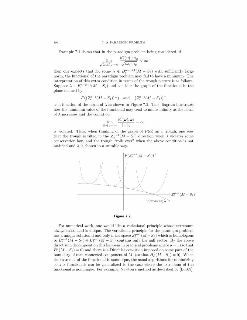
196 7. A PARADIGM PROBLEM
Example 7.1 shows that in the paradigm problem being considered, if
lim√〈ω,ω〉p→∞
〈C(ω), ω〉p√〈ω, ω〉p
<∞
then one expects that for some λ ∈ Bn−p+1c (M − S2) with sufficiently large
norm, the functional of the paradigm problem may fail to have a minimum. Theinterpretation of this extra condition in terms of the trough picture is as follows.Suppose λ ∈ Bn−p+1
c (M − S2) and consider the graph of the functional in theplane defined by
F((Zp−1
c (M − S1))⊥)
and(Zp−1c (M − S1)
)⊥
as a function of the norm of λ as shown in Figure 7.2. This diagram illustrateshow the minimum value of the functional may tend to minus infinity as the normof λ increases and the condition
lim‖ω‖p→∞
〈C(ω), ω〉‖ω‖p
=∞
is violated. Thus, when thinking of the graph of F (α) as a trough, one seesthat the trough is tilted in the Zp−1
c (M − S1) direction when λ violates someconservation law, and the trough “rolls over” when the above condition is notsatisfied and λ is chosen in a suitable way.
F (Zp−1c (M − S1))
⊥
Zp−1c (M − S1)
increasing λ
Figure 7.2.
For numerical work, one would like a variational principle whose extremumalways exists and is unique. The variational principle for the paradigm problemhas a unique solution if and only if the space Zp−1
c (M−S1) which is homologousto Bp−1
c (M − S1)⊕Hp−1c (M − S1) contains only the null vector. By the above
direct sum decomposition this happens in practical problems where p = 1 (so thatB0c (M −S1) = 0) and there is a Dirichlet condition imposed on some part of the
boundary of each connected component of M , (so that H0c (M −S1) = 0). When
the extremal of the functional is nonunique, the usual algorithms for minimizingconvex functionals can be generalized to the case where the extremum of thefunctional is nonunique. For example, Newton’s method as described by [Lue69],

7D. MODIFIED VARIATIONAL PRINCIPLES 197
Section 10.4 can be generalized as in [Alt55]. However, in such cases it is usuallyeasier to reformulate the variational principle for the paradigm problem in sucha way that there always exist a unique solution. There are two basic approachesto this problem which will be considered next.
7D. Modified Variational Principles
The purpose of this section is to formulate variational principles for the par-adigm problem for which the potential α is unique. Such variational principleswill have interesting consequences for conservation laws since a unique solutionfor the potential α implies that there is no gauge transformation which in turnimplies that there is no conservation law which is naturally associated with thefunctional.
The first approach to the problem is to note that once the principal boundaryconditions have been imposed on S1 the space of admissible variations of theextremal is Cp−1
c (M −S1) and the space of gauge transformations is Zp−1c (M −
S1). Hence, if the space of admissible variations of the functional and the domainof the functional is restricted to
(Zp−1c (M − S1)
)⊥ ∩ Cp−1c (M − S1),
the functional’s previous minimum can still be attained but the solution is nowunique. By the orthogonal decomposition developed in Section MA-M, one has
(Zp−1c (M − S1))
⊥ = Bp−1(M,S2)
hence the space of admissible variations becomes
Bp−1(M,S2) ∩ Cp−1c (M − S1) =
α∣∣ tα = 0 on S1, α = δpω in M for some ω ∈ Cpc (M) with nω = 0 on S2
.
This procedure raises an interesting question. By the observations of [Ton68]one knows that the number of degrees of freedom in the gauge transformation isequal to the number of degrees of freedom by which the source, described by λ,is constrained by a conservation law. Hence in this case where the domain of thefunctional is constrained, so that the extremal is unique, one expects that thevariational principle is completely insensitive to violations of the conservation lawλ ∈ Bn−p+1
c (M − S2). To see why this is so, consider the unique decomposition
λ = λcons + λnonc,
where
λ ∈ Cn−p+1c (M), λcons ∈ Bn−p+1
c (M − S2), λnonc ∈ (Bn−p+1c (M − S2))
⊥.
What is required is to show that the extremal of the functional is independent ofthe way in which λnonc is prescribed. Considering the functional of the paradigm

198 7. A PARADIGM PROBLEM
problem as a function of λ, when α is restricted as above, one has
Fλ(α)− Fλcons(α) = (−1)p−1
∫
M
α ∧ λnonc
= (−1)(p−1)−(n−p+1)(p−1)
∫
M
λnonc ∧ α
= (−1)(p−1)
∫
M
λnonc ∧ ∗∗α = (−1)(p−1) 〈λnonc, ∗α〉n−p+1 .
However, while
∗α ∈ ∗((Zp−1
c (M − S1))⊥)
= ∗Bp−1(M,S2) = Bn−p+1c (M − S2),
we also have
λnonc ∈(Bn−p+1c (M − S2)
)⊥,
and combining these two results, we get
〈λnonc, ∗α〉n−p+1 = 0,
so that
Fλ(α) = Fλcons(α).
Thus, by restricting the class of admissible variations of the functional’s extremal,one obtains a variational formulation whose unique extremal is insensitive toviolations of the compatibility condition λ ∈ Bn−p+1(M − S1). This approachto the problem is useful in the context of direct variational methods such as theRitz method or the finite element method only when it is possible to find basisfunctions which ensure that
α ∈(Zp−1c (M − S1)
)⊥= Bp−1(M,S2).
The second method for obtaining a variational formulation of the paradigmproblem in which the extremal is unique is inspired by [Kot82] chapter 5. Inthis method, which at first sight resembles the “penalty function method” (see[Lue69], sect. 10.11), the domain of the functional before principal boundaryconditions are imposed is Cp−1
c (M). The method involves finding a functionalF⊥(α) whose graph looks like a trough perpendicular to the trough of F (α):
In this scheme the functional
G(α) = F (α) + F⊥(α)
has a unique minimum which lies above the (Zp−1c (M − S1))
⊥ “axis” wheneverthe trough associated with F (α) is not tilted. That is if F⊥(α) is designed sothat its minimum is the (Zp−1
c (M − S1))⊥ “axis” then the minimum of G(α)
should lie above the (Zp−1c (M − S1))
⊥ “axis” whenever λ ∈ Bn−p+1c (M − S2).
It is also desired that the contrapositives of these statements are also true inthe following sense. If λ 6∈ Bn−p+1
c (M − S2) so that the trough associated withF (α) is “tilted” then the distance of the extremum of the functional G(α) tothe G(α) − (Zp−1
c (M − S1))⊥ plane measures, in some sense, the value of the
projection
‖αG‖−1p−1 max
αG∈Zp−1c (M−S1)
∫
M
αG ∧ λ.

7D. MODIFIED VARIATIONAL PRINCIPLES 199
Value of functional
`Zp−1
c (M − S1)´⊥
Zp−1c (M − S1)
Figure 7.3. The troughs associated with F (α) (on the Zp−1c (M − S1) axis) and
F⊥(α).
Having this picture in mind, the first thing to do is construct a functionalwith the properties desired of F⊥(α). To find a functional which is definite onZp−1c (M − S1) and level on (Zp−1
c (M − S1))⊥, one notes that the orthogonal
decomposition of Section MA-M gives(Zp−1c (M − S1)
)⊥= Bp−1(M,S2), Zp−1
c (M − S1) =(Bp−1(M,S2)
)⊥.
Hence, one actually wants a functional F⊥(α) which is level on Bp−1(M,S2) and
convex on (Bp−1(M,S2))⊥.
As a prelude to the construction of F⊥(α), let K be a map
K : Cp−2(M)→ Cp−2(M)
satisfying the same conditions associated with the constitutive mapping. Thatis, for ω, ω1, ω2 ∈ Cp−2(M) the following three properties are assumed to hold.
(1) Strict monotonicity:
〈K(ω1)−K(ω2), ω1 − ω2〉p−2 ≥ 0,
with equality if and only if ω1 = ω2.(2) Symmetry: defining the functional
fω(ω1) = 〈K(ω), ω1〉p−2
and denoting the Gateaux variation of this functional by
f ′ω(ω1, ω2) = 〈K ′ω(ω2), ω1〉p−2 ,
it is required that this function is a symmetric bilinear function of ω1 andω2. That is
〈K ′ω(ω1), ω2〉p−2 = 〈K ′
ω(ω2), ω1〉p−2 .
(3) Asymptotic property:
lim‖ω‖p−2→∞
〈K(ω), ω〉p−2
‖ω‖p−2=∞.

200 7. A PARADIGM PROBLEM
In addition to these usual properties the mapping K will also be assumed tosatisfy the condition K(0) = 0, where 0 is the differential form whose coefficientsvanish relative to any basis.
Given a mapping K which satisfies the above four conditions, consider the
functional F0 : Cp−1(M,S2)→ R defined by
F0 (γ(1)) = F0 (γ(0)) +
∫ 1
0
⟨K (δγ(s)) ,
d
ds(δγ(s))
⟩
p−2
ds
for any γ : [0, 1] → Cp−1(M,S2). By construction, this functional is convex inthe subspace (
Zp−1(M,S2))⊥ ∩ Cp−1(M,S2)
and “level” in the subspace Zp−1(M,S2). Furthermore, F0(α) ≥ F0(0) with
equality if and only if α ∈ Zp−1(M,S2).At this stage, the construction of F⊥(α) is actually simple. Considering the
orthogonal decomposition of Section MA-M, the following diagrams are readilyseen to be true:
(7–3)
Bp−1c (M − S1) ⊂ Zp−1
c (M − S1) = Bp−1c (M − S1) ⊕Hp−1(M,S1)
‖ ‖ ‖ ‖(Zp−1(M,S2)
)⊥⊂(Bp−1(M,S2)
)⊥=(Zp−1(M,S2)
)⊥⊕Hp−1(M,S1)
and(7–4)
Bp−1(M,S2) ⊂ Zp−1(M,S2) = Bp−1(M,S2) ⊕Hp−1(M,S1)
‖ ‖ ‖ ‖(Zp−1c (M − S1)
)⊥⊂(Bp−1c (M − S1)
)⊥=(Zp−1c (M − S1)
)⊥⊕Hp−1(M,S1)
where
∗Hn−p+1(M,S2) = Hp−1(M,S1) = Zp−1c (M − S1) ∩ Zp−1(M,S2).
Looking at these diagrams, we see that in (7–3) F⊥ is supposed to be convexon the spaces listed in the second column while F0 is convex in the spaces listedin the first column. Similarly, in (7–4), F⊥ is invariant with respect to varia-tions in the spaces listed in the first column while F0 is invariant with respectto variations in the spaces listed in the second column. Thus, observing thedirect sum decompositions in the third column of (7–3) and (7–4) it is obviousthat the functional F0 meets all of the specifications of F⊥ except on the spaceHp−1(M,S1). More specifically, the functional F⊥ is required to constrain theperiods of a p − 1 form in Hp−1(M,S1) while the functional F0 does not. Tofix this discrepancy, let zi, with 1 ≤ i ≤ βn−p+1(M,S2), be a set of generatorsof Hn−p+1(M,S2), and let ki, with 1 ≤ i ≤ βn−p+1(M,S2), be a set of positiveconstants. For a curve
γ : [0, 1]→ Cp−1c (M),

7D. MODIFIED VARIATIONAL PRINCIPLES 201
the functionalsFi : Cp−1
c (M)→ R, 1 ≤ i ≤ β1(M,S1),
defined by
Fi
(γ(1)
)= Fi
(γ(0)
)+ ki
∫ 1
0
(∫
zi
∗γ(s))(∫
zi
∗∂γ(s)∂s
)ds
= Fi
(γ(0)
)+ki2
((∫
zi
∗γ(1)
)2
−(∫
zi
∗γ(0)
)2)
have the propertyFi(α) ≥ Fi(0),
with equality if and only if the integral of ∗α over zi vanishes. Next, considerthe “candidate” functional
F⊥cand(α) =
βn−p+1(M,S2)∑
i=0
Fi(α).
Immediately, from the definitions of the Fi, one has
F⊥cand(α)− F⊥
cand(0) =
βn−p+1(M,S2)∑
i=0
(Fi(α)− Fi(0)) ≥ 0,
with equality if and only if
Fi(α) = Fi(0), 0 ≤ i ≤ βn−p+1(M,S2).
This last condition is equivalent to
α ∈ Zp−1(M,S2) and
∫
zi
∗α = 0 for 1 ≤ i ≤ βn−p+1(M,S2),
or
∗α∈∗Zp−1(M,S2)=Zn−p+1c (M−S2),
∫
zi
∗α=0 for 1≤ i≤βn−p+1(M,S2).
By the relative de Rham isomorphism, this is equivalent to
∗α ∈ Bn−p+1c (M − S2)
which in turn is equivalent to
α ∈ ∗Bn−p+1c (M − S2) = Bp−1(M,S2) =
(Zp−1c (M − S1)
)⊥.
Hence, in summary,F⊥
cand(α)− F⊥cand(0) ≥ 0,
with equality if and only if
α ∈(Zp−1c (M − S1)
)⊥.
Furthermore, by construction, F⊥cand is convex when its domain is restricted to
the space Zp−1c (M − S1). Thus interpreting F⊥
cand as a trough, it is seen that itsatisfies the requirements of F⊥ and hence can be used to define F⊥. Hence, fora curve
γ : [0, 1]→ Cp−1(M,S2),

202 7. A PARADIGM PROBLEM
one can define the functional
F⊥ : Cp−1(M,S2)→ R
as follows:
F⊥ (γ(1))− F⊥ (γ(0)) = F⊥cand (γ(1))− F⊥
cand (γ(0))
=
βn−p+1(M,S2)∑
i=0
(Fi (γ(1))− Fi (γ(0)))
=
∫ 1
0
⟨K (δγ(s)) , δ
(∂γ(s)
∂s
)⟩
p−2
ds
+
βn−p+1(M,S2)∑
i=1
ki
∫ 1
0
(∫
zi
∗γ(s))(∫
zi
∗∂γ(s)∂s
)ds.
Finally one can complete the quest for a variational formulation of the paradigmproblem in which the extremal of the functional is unique by letting
G(α)−G(0) = (F (α)− F (0)) +(F⊥(α)− F⊥(0)
),
while respecting the principal boundary conditions
tα prescribed on S1, nα = 0 on S2.
Explicit Variation of the Modified Variational Principle. To define G(α)more explicitly, consider a continuous differentiable curve
γ : [0, 1]→ Cp−1(M,S2)
with
γ(0) = α0 an initial state,
γ(1) = α1 an extremal;
and, in order to respect the principal boundary conditions,
tα0 = tα = tγ(s) on S1,
nα0 = nα = nγ(s) = 0 on S2,
for all s ∈ [0, 1]. No other constraints are placed on γ, so that
∂γ
∂s∈ Cp−1(M,S2) ∩ Cp−1
c (M − S1) for all s ∈ [0, 1]
and the variation of the extremal
∂γ
∂s
∣∣∣∣s=1
= α
can be chosen to be any admissible variation where the space of admissible
variations is Cp−1(M,S2)∩Cp−1c (M−S1). Thus writing out the functional G(α)
7D. MODIFIED VARIATIONAL PRINCIPLES 203
explicitly one has
G(α)−G(α0) = G(γ(1))−G(γ(0))
=
∫ 1
0
(⟨C(dγ(s)),
∂
∂sdγ(s)
⟩p
+ (−1)r⟨∗λ, ∂γ(s)
∂s
⟩p−1
+⟨K(δγ(s)),
∂
∂s(δγ(s))
⟩p−2
)ds
+
βn−p+1(M,S2)∑
i=1
ki
∫ 1
0
(∫
zi
∗γ(s))(∫
zi
∗∂γ(s)∂s
)ds,
where r = (n− p+1)(p− 1) + (p− 1). To investigate the stationary point of thefunctional one recalls that
α = γ(1) ∈ Cp−1c (M − S1), α =
∂γ
∂s
∣∣∣∣s=1
∈ Cp−1c (M − S1) ∩ Cp−1(M,S2),
and insists that∂
∂εG (γ(1− ε))
∣∣∣∣ε=0
= 0
for all admissible α. Doing this shows that the following identity must be truefor all α:
(7–5) 0 =⟨C(dα), dα
⟩p
+ (−1)r⟨∗λ, α
⟩p−1
+⟨K(δα), δα
⟩p−2
+
βn−p+1(M,S2)∑
i=1
(∫
zi
∗α)(∫
zi
∗α).
It is in general not possible to integrate by parts to obtain an Euler–Lagrangeequation in the usual sense because of the integral terms which constrain theintegrals of ∗α on a set of generators of Hn−p+1(M,S2). Furthermore, in thepresent case it is not necessary to derive an Euler–Lagrange equation since thefunctional is designed to be extremized by direct variational methods. What isnecessary to verify is the geometric picture developed when thinking about thetroughs associated with the graphs of the functionals F (α) and F⊥(α). That is,it must be verified that when λ obeys the conservation law
λ ∈ Bn−p+1c (M − S2)
the extremal of G(α) provides a physically meaningful solution to the paradigmproblem and the projection of the extremal into Zp−1
c (M − S1) vanishes. Alter-natively, when the conservation law is violated one hopes that the extremal ofG(α) can be interpreted as providing a “least squares” solution to the nearestphysically meaningful problem where the conservation law is not violated andthat the projection of the extremal into Zp−1
c (M − S1) measures in some sensethe extent by which the conservation law is violated. Hence let λ be prescribedin some way which does not necessarily respect a conservation law and considerthe orthogonal decomposition
λ = λcons + λnonc,

204 7. A PARADIGM PROBLEM
where
λcons ∈ Bn−p+1c (M − S2)
λnonc ∈(Bn−p+1c (M − S2)
)⊥= Zn−p+1(M,S1).
From this orthogonal decomposition, it follows immediately that
∗λ = ∗λcons + ∗λnonc,
where
∗λcons = ∗Bn−p+1c (M − S2) = Bp−1(M,S2),
∗λnonc = ∗Zn−p+1(M,S1) = Zp−1c (M,S1).
Similarly, for α ∈ Cp−1(M,S2) one has the orthogonal decomposition
Cp−1(M,S2) = Bp−1(M,S2)⊕(Zp−1c (M − S1) ∩ Cp−1 (M,S2)
),
and α can be expressed as
α = α0 + αG,
where
α0 ∈ Bp−1(M,S2),
αG ∈ Zp−1c (M − S1) ∩ Cp−1(M,S2).
Finally, for α ∈ Cp−1(M,S2) ∩Cp−1c (M − S1) one has the orthogonal decompo-
sition
Cp−1(M,S2) ∩ Cp−1c (M − S1)
=(Bp−1(M,S2) ∩ Cp−1
c (M − S1))⊕(Zp−1c (M − S1) ∩ Cp−1(M,S2)
),
and α can be expressed as
α = α0 + αG,
where
α0 ∈ Bp−1(M,S2) ∩ Cp−1c (M − S1),
αG ∈ Zp−1c (M − S1) ∩ Cp−1(M,S2).
Before returning to the condition that ensures that the functional G is stationaryat α, note that expressing α0 and α0 as
α0 = δθ, α0 = δθ
it becomes apparent that∫
zi
∗α0 =
∫
zi
∗δθ = (−1)p∫
zi
d ∗ θ = 0, 1 ≤ i ≤ βn−p+1(M − S2),
∫
zi
∗α0 =
∫
zi
∗δθ = (−1)p∫
zi
d ∗ θ = 0, 1 ≤ i ≤ βn−p+1(M − S2),

7D. MODIFIED VARIATIONAL PRINCIPLES 205
since the integral of a coboundary on a cycle vanishes. Next recall the identity
(7–5) which must be satisfied for all α ∈ Cp−1c (M − S1) ∩ Cp−1(M,S2) in order
for the functional G to be stationary at α:
0 = 〈C(dα), dα〉p + 〈K(δα), δα〉p−2 + (−1)r 〈∗λ, α〉p−1
+
βn−p+1(M,S2)∑
i=1
ki
(∫
zi
∗α)(∫
zi
∗α).
Substituting the earlier orthogonal decompositions into this identity and recallingthe definitions of the spaces involved gives
0 = 〈C(dα0), dα0〉p +⟨K(δαG), δαG
⟩p−2
+ (−1)r⟨∗λcons + ∗λnonc, α0 + αG
⟩p−1
+
βn−p+1(M,S2)∑
i=1
ki
(∫
zi
∗αG)(∫
zi
∗αG).
Keeping in mind that the spaces Zp−1c (M − S1) and Bp−1(M,S2) are mutually
orthogonal, the inner product involving the source term and the variation of theextremal can be simplified to yield
0 =⟨C(dα0), dα0
⟩p
+ (−1)r⟨∗λcons, α0
⟩p−1
+⟨K(δαG), δαG
⟩p−2
+ (−1)r⟨∗λnonc, αG
⟩p−1
+
βn−p+1(M,S2)∑
i=1
ki
(∫
zi
∗αG)(∫
zi
∗αG).
It is obvious by the independence of α0 and and αG that the above condition isequivalent to the following two conditions:
(7–6) 0 = 〈C(dα0), dα0〉p + (−1)r 〈∗λcons, α0〉p−1 ,
for all α0 ∈ Bp−1(M,S2) ∩ Cp−1c (M − S1), and
(7–7) 0 = 〈K(δαG), δαG〉p−2 + (−1)r 〈∗λnonc, αG〉p−1
+
βn−p+1(M,S2)∑
i=1
(∫
zi
αG
)(∫
zi
αG
),
for all α ∈ Zp−1c (M−S1)∩Cp−1(M,S2). To deduce the properties of the extremal
α = α0 +αG of the functional G, one can look at the consequences of the abovetwo identities. This can be done in two steps as follows.
Consequences of condition (7–6). Condition (7–6) is precisely the criterion forthe original functional F to be stationary at α0 ∈ (Zp−1
c (M − S1))⊥ and where
the source is λcons. Previous calculations show that the above identity implies
d ∗ C(dα0) = λcons in M,
t ∗ C(dα0) = 0 in S2,

206 7. A PARADIGM PROBLEM
so that the potential that makes G(α) stationary gives a solution to the paradigmproblem where λ is replaced by λcons. By the definition of λcons it follows that
minξ∈Bn−p+1
c (M−S2)‖ λ− ξ ‖n−p+1=‖ λ− λcons ‖n−p+1 .
Hence one can say that the extremal of G provides a solution to the nearestphysically meaningful paradigm problem.
Consequences of condition (7–7). Noticing that αG and αG both belong to
the space Zp−1c (M −S1)∩ Cp−1(M,S2) and that αG is arbitrary, one can let αG
be equal to αG, so that the identity (7–7) becomes
−(−1)r 〈∗λnonc, αG〉p−1 = 〈K(δαG), δαG〉p−2 +
βn−p+1(M,S2)∑
i=1
ki
(∫
zi
∗αG)2
≥ 0,
with equality if and only if αG ∈ Bp−1(M,S2). Since αG is an element ofZp−1c (M − S1) it is seen that the expression becomes an equality if and only if
αG = 0. Thus it is apparent that
∗λnonc = 0 implies αG = 0
and that
αG 6= 0 implies ∗λnonc 6= 0.
To prove the converses of these statements it is necessary to show that it ispossible to find a αG such that if λnonc 6= 0 then
〈∗λnonc, αG〉p−1 6= 0
and that αG is such an αG. Unfortunately,
∗λnonc ∈ Zp−1c (M − S1)
and
αG ∈ Zp−1c (M − S1) ∩ Cp−1(M,S2);
hence αG can be selected to reflect the projection of λnonc in Zp−1c (M − S1) ∩
Cp−1(M,S2) and nothing more. Note, however, that if one imposes with com-plete certainty tλ = 0 on S2, then λ ∈ Cn−p+1
c (M − S2) and hence
∗λnonc ∈ ∗Zn−p+1(M,S1) ∩ ∗Cn−p+1c (M − S2) = Zp−1
c (M − S1) ∩ Cp−1(M,S2).
In this case αG, αG and ∗λnonc all belong to the space
Zp−1c (M − S1) ∩ Cp−1(M,S2)
and it is always possible to find an αG such that ∗λnonc 6= 0 implies
〈∗λnonc, αG〉p−1 6= 0.
However, by Equation (7–7) this implies that αG 6= 0 and since Equation (7–7)is valid for all possible αG, one can set αG equal to αG to obtain
−(−1)r〈∗λnonc, αG〉p−1 = 〈K(δαG), δαG〉p−2 +
βn−p+1(M,S2)∑
i=1
ki
(∫
zi
∗αG)2
> 0.
7E. TONTI DIAGRAMS 207
Hence λnonc 6= 0 implies αG 6= 0, or αG = 0 implies λnonc = 0, and it is provedthat
αG = 0 if and only if ∗λnonc = 0.
It is seen that the identities (7–6) and (7–7) adequately describe what happens
in a neighborhood of the extremal α in Cp−1(M,S2) when one thinks in termsof tilted troughs.
Two final points are in order. The first point is that the value of the func-tional F⊥ evaluated at the extremal of G provides an a posteriori estimate ofhow large λnonc is. This is apparent from the trough picture. The second pointis that when there is a pseudo-Riemannian structure on the manifold M , theexpression 〈·, ·〉k is no longer positive definite, hence the functionals consideredare no longer convex and the trough picture is no longer valid. Although theorthogonal decomposition of Section MA-M is still a legitimate direct sum de-composition and when βn−p+1(M,S2) = 0 the functional G still provides aneffective way of imposing the Lorentz gauge δα = 0 whenever the conservationof charge (dλ = 0) is respected, it is not clear what the exact properties of G are.From the point of view of computational electromagnetics, there is little motiva-tion for pursuing this question and so the case of pseudo-Riemannian structuresis ignored.
7E. Tonti Diagrams
In this final section, Tonti diagrams and the associated framework for com-plementary variational principles will be considered. This work is well known topeople in the field of computational electromagnetics and an overview of the liter-ature in this context is given in the paper by Penmann and Fraser [PF84]. In thisconnection the author also found the seminar paper by [Cam83] most useful. Thebasis of the following discussion are the papers of Enzo Tonti [Ton72b, Ton72a]where certain short exact sequences associated with differential operators appear-ing in field equations are recognized as being a basic ingredient in formulatinga common structure for a large class of physical theories. This work of Tontifits hand in glove with the work of J. J. Kohn [Koh72] on differential complexes.The point of view taken here is that for the practical problems described bythe paradigm problem being considered in this chapter, the interrelationship be-tween the work of Tonti and Kohn is easily seen by considering the complexesassociated with the exterior derivative and its adjoint on a Riemannian man-ifold with boundary. The idea of introducing complexes and various conceptsfrom algebraic topology into Tonti diagrams is not new and is developed in thecompanion papers [Bra77] and [Ton77].
The main conclusion to be drawn from the present approach is that the dif-ferential complexes associated with the exterior derivative give, when applica-ble, a deeper insight into Tonti diagrams than is usually possible since the deRham isomorphism enables one to give concrete and intuitive answers to ques-tions involving the (co)homology of the differential complexes. More precisely,the usual development of Tonti diagrams involves differential complexes wherethe symbol sequence of the differential operators involved is exact while what

208 7. A PARADIGM PROBLEM
is actually desired is that the (co)homology of the complex be trivial. Thatis, if the (co)homology of the differential complex is nontrivial, then reasoningwith the exactness of the symbol sequence alone may lead to false conclusionsconcerning the existence and uniqueness of solutions to equations. To the bestof the author’s knowledge, the only differential complexes of practical use forwhich something concrete can be said about (co)homology, are the differentialcomplexes associated with the exterior derivative since in this case the de Rhamisomorphism applies.
To formulate a Tonti diagram for the paradigm problem, consider first theparadigm problem and suppose that Hp−1
c (M − S1) is trivial. In this case,
Zp−1c (M − S1) = Bp−1
c (M − S1)
and
α→ α+ dχ, χ ∈ Cp−2c (M − S1)
is a gauge transformation describing the nonuniqueness in the potential α. Next,when dealing with complementary variational principles, we must find an
ηpart ∈ Cn−pc (M − S2) = ∗Cp(M,S2)
such that
dηpart = λ
and
η − ηpart ∈ Bn−pc (M − S2) = ∗Bp(M,S2).
In this case the forms β and η are determined by reducing the problem to aboundary value problem for
ν ∈ Cn−p−1c (M − S2) = ∗Cp+1(M,S2),
where ν is defined by
dν = η − ηpart.
This boundary value problem for ν is deduced from the equations
dβ = 0 in M
tβ = 0 on S1
dν + ηpart = ∗C(β) in M .
From these equations the boundary value problem is seen to be
d(C−1
((−1)p(n−p) ∗
(ηpart + dν
)))= 0 in M
t(C−1
((−1)p(n−p) ∗
(ηpart + dν
)))= 0 on S1
tν = 0 on S2.
The variational formulation for this problem is obtained by considering a curve
γ : [0, 1]→ Cn−p−1c (M − S2)

7E. TONTI DIAGRAMS 209
and defining the functional for the complementary problem as follows:
J(γ(1))− J(γ(0))
= −(−1)p(n−p)∫ 1
0
⟨C−1
((−1)p(n−p) ∗ (ηpart + dγ(s))
), ∗(ηpart + d
∂γ(s)
∂s
)⟩
p
ds
= −∫ 1
0
∫
M
(C−1
((−1)p(n−p) ∗(ηpart + dγ(s))
))∧(ηpart + d
∂γ(s)
∂s
)ds.
To verify that this is indeed the correct functional let
γ(1) = ν,∂γ(s)
∂s
∣∣∣∣s=1
= ν
be the extremal and any variation of the extremal of the functional where the
space of admissible variations is Cn−p−1c (M − S2) = ∗Cp+1(M,S2). The func-
tional is stationary when
∂J
∂εγ(1− ε)
∣∣∣∣ε=0
= 0
for all admissible variations of the extremal. This condition amounts to
0 =
∫
M
C−1((−1)p(n−p) ∗ (ηpart + dγ(1))
)∧ d(∂γ(s)
∂s
∣∣∣∣s=1
)
or
0 =
∫
M
C−1((−1)p(n−p) ∗ (ηpart + dν)
)∧ dν
for all admissible ν. Integrating this expression by parts and using the fact that
tν = 0 on S2,
one obtains
0 =
∫
M
d(C−1
((−1)p(n−p) ∗ (ηpart + dν)
))∧ ν
−∫
S1
t(C−1
((−1)p(n−p) ∗ (ηpart + dν)
))∧ tν,
from which it is apparent that the functional is the desired one since ν canbe taken to be any admissible variation. In this formulation, the extremal ofthe functional J is unique up an to an element of Zn−p−1
c (M − S2) and thenonuniqueness can be described by a gauge transformation
ν → ν + νG, where νG ∈ Zn−p−1c (M − S2).
Hence whenever there is a Riemannian structure on M which induces the innerproduct 〈 · , · 〉k on k-forms, the functional J is convex on
(Zn−p−1c (M − S2))
⊥ = Bn−p−1(M,S1) = ∗Bp+1c (M − S1)
and level on the space
Zn−p−1c (M − S2) = ∗Zp+1(M,S2).
210 7. A PARADIGM PROBLEM
Just as the construction of a functional F⊥ enabled one to modify the functionalF in order to construct a variational formulation involving a functional
G(α) = F (α) + F⊥(α)
for which the resulting extremal is unique, one can construct a functional J⊥(ν)such that
I(ν) = J(ν) + J⊥(ν)
is a functional whose unique extremal is also an extremal of the functional J .This, of course, happens when the functional J⊥ is constructed so that it isconvex on the space
Zn−p−1c (M − S2) = ∗Zp+1(M,S2)
and level on
(Zn−p−1c (M − S2))
⊥ = Bn−p−1(M,S1) = ∗Bp+1c (M − S1).
Thus, again, one is led to a situation involving two troughs as shown in Figure 7.3.With this picture in mind, the functional J⊥ can be constructed in analogy withthe construction of F⊥. Consider first a mapping
K ′ : Cn−p−2(M)→ Cn−p−2(M)
which satisfies the same symmetry, monotonicity, and asymptotic properties re-quired of the function K used in the construction of F⊥. Define a functional J⊥
as follows. Given
γ : [0, 1]→ Cn−p−1(M,S1),
let
J⊥ (γ(1))− J⊥ (γ(0)) = −∫ 1
0
⟨K ′−1 (δγ(s)) , δ
∂γ(s)
∂s
⟩
n−p−2
−βp+1(M,S1)∑
i=0
li
∫ 1
0
(∫
zi
∗γ(s))(∫
zi
∗∂γ(s)∂s
)ds,
where the zi are associated with generators of the homology group Hp+1(M,S1)and the li are positive constants. The functional J⊥ thus defined is convex onthe space
Zn−p−1c (M − S2) =
(Bn−p−1(M,S1)
)⊥
and level on the space(Zn−p−1c (M − S2)
)⊥= Bn−p−1(M,S1).
This is easily seen, since the situations involving F⊥ and J⊥ become identical ifone interchanges the symbols
J⊥ ↔ F⊥,
S1 ↔ S2,
K ′ ↔ K,
n− p↔ p.

7E. TONTI DIAGRAMS 211
Hence the functional I defined as
I(ν) = J(ν) + J⊥(ν),
with domain Cn−p−1(M,S1) ∩ Cn−p−1c (M − S2), has a unique extremum.
Finally, in order to finish this prelude to the Tonti diagram, note that if
βn−p−1(M,S2) = 0
the nonuniqueness in the complementary potential ν, when the variational for-mulation involving the functional J is used, can be described by a gauge trans-formation
ν → ν + dθ,
where
θ ∈ Cn−p−2c (M − S2) = ∗Cp+2(M,S2).
Furthermore, when considering the Tonti diagram it is convenient to assume thatβ may be related to some type of source ρ through the equation
dβ = ρ,
where in the present case ρ = 0. Hence, in terms of the notation introducedso far, the above formulation of the complementary variational principle for theparadigm problem is summarized by the Tonti type diagram in Figure 7.4 andused extensively in [PF84]. For the present purpose, the diagram in Figure 7.4presents a simplistic view of the paradigm problem since boundary conditions
ξ
dp−3
?dλ
dn−p+2
6
α
dp−2
? primal - λ
dn−p+16
β
dp−1
?∗C - η
dn−p6
ρ
dp
? dual
ν
dn−p−16
dρ
dp+1
?θ
dn−p−26
dp+2
?
dn−p−36
Figure 7.4. Typical Tonti diagram.

212 7. A PARADIGM PROBLEM
and domains of definition of operators have been ignored. Thus it is impossi-ble to get a clear understanding of how homology groups come into play. Toremedy this situation, one must realize that when boundary conditions are im-posed, the left hand side of the above diagram is associated with the complexC∗c (M − S1) while the right hand side of the diagram is associated with the
complex C∗c (M − S2) = ∗C∗(M,S2). Thus to be more explicit, the above dia-
gram should be rewritten as shown in Figure 7.5. Once this structure has been
Cp−2c (M − S1)
dp−3
?Cn−p+2c (M − S2)
dn−p+26
'Cp−2(M,S2)
δp−2
6
Cp−1c (M − S1)
dp−2
?Cn−p+1c (M − S2)
dn−p+16
'Cp−1(M,S2)
δp−16
Cpc (M − S1)
dp−1
?∗C- Cn−pc (M − S2)
dn−p6
' Cp(M,S2)
δp
6
Cp+1c (M − S1)
dp
?Cn−p−1c (M − S2)
dn−p−16
'Cp+1(M,S2)
δp+16
Cp+2c (M − S1)
dp+1
?Cn−p−2c (M − S2)
dn−p−26
'Cp+2(M,S2)
δp+26
dp+2
?
dn−p−36δp+3
6
Figure 7.5. Fortified Tonti diagram.
identified, it is apparent from the previous sections of this chapter that questionsof existence and uniqueness of potentials and questions of existence and unique-ness of solutions to boundary value problems are easily handled by using theorthogonal decomposition developed in Section MA-M. Though these questionshave been considered in detail in the case of the potential α and the results forthe complementary potential ν follow analogously, it is useful to outline the roleplayed by various cohomology groups. Specifically, the role of the following pairsof groups and isomorphisms will be summarized:
Hp−1c (M − S1) ' Hn−p+1
c (M − S2)(7–8)
Hpc (M − S1) ' Hn−p
c (M − S2)(7–9)
Hp+1c (M − S1) ' Hn−p−1
c (M − S2)(7–10)
Consequences of (7–8). Once tα is prescribed on S1, the group Hp−1c (M−S1)
was seen to describe the nonuniqueness of α in the paradigm problem which

7E. TONTI DIAGRAMS 213
cannot be described by a gauge transformation of the form
α→ α+ dχ, χ ∈ Cp−2c (M − S1).
In other words, the nonuniqueness of α is described by Zp−1c (M − S1) while
the above gauge transformation involves Bp−1c (M − S1), hence the difference is
described by Hp−1c (M − S1) since by definition
Hp−1c (M − S1) = Zp−1
c (M − S1)/Bp−1c (M − S1).
Dually, Hn−p+1c (M − S2) was seen to be associated with the global conditions
ensuring that λ ∈ Bn−p+1c (M − S2) once it is known that λ ∈ Zn−p+1
c (M − S2).Finally, the isomorphism
Hp−1c (M − S1) ' Hn−p+1
c (M − S2)
expresses the duality between the global degrees of freedom in the nonuniqueness(gauge transformation) of α and the solvability condition (conservation law)involving λ. This isomorphism is exploited in the construction of the functionalF⊥ and its interpretation is best appreciated by using the de Rham isomorphismto reduce the above isomorphism to
Hp−1(M,S1) ' Hn−p+1(M,S2)
and to interpret this isomorphism in terms of the intersection numbers of thegenerators of these two homology groups as in Chapter 1.
Consequences of (7–9). The group Hpc (M − S1) is associated with global
conditions which ensure that β ∈ Bpc (M − S1) once it is determined that β ∈
Zpc (M − S1). Furthermore, it gives insight into the conditions which α mustsatisfy on S1 if β = dα. Dually the groupHn−p
c (M−S2) is associated with globalconditions which ηpart must satisfy in order for there to be a ν ∈ Cn−p−1
c (M−S2)such that
dηpart = λ in M ,
dν = η − ηpart in M .
Thus the cohomology group Hpc (M − S1) is used in formulating a primal vari-
ational principle, while the cohomology group Hn−pc (M − S2) is used in formu-
lating a dual variational principle and the isomorphism
Hpc (M − S1) ' Hn−p
c (M − S2)
then expresses the fact that the number of global conditions is the same in boththe original and complementary formulations. Note that for most problems, theperiods of closed forms on the generators of
Hp(M,S1), Hn−p(M,S2)
have the interpretation of a lumped parameter current, potential difference, orflux as was seen in Examples 1.14, 1.15, 2.3, and 2.4. Thus in these examplesthe isomorphism in homology has a direct interpretation.

214 7. A PARADIGM PROBLEM
Consequences of (7–10). Had β not been a closed form but rather tied to anequation of the form
dβ = ρ,
then if ρ ∈ Zp+1c (M − S1) the group Hp+1
c (M − S1) is associated with theconditions which ensure that ρ ∈ Bp+1
c (M−S1). Thus the groupHp+1c (M−S1) is
associated with the global conditions which ensure the solvability of the equationsfor the extremal ν of the complementary variational principle. Dually, the groupHn−p−1c (M − S2) describes the nonuniqueness in ν which cannot be described
by a gauge transformation of the form
ν → ν + dθ, θ ∈ Cn−p−2c (M − S2).
In other words, the nonuniqueness of ν is described by Zn−p−1c (M − S2) while
the above gauge transformation involves Bn−p−1c (M − S2) and the difference is
characterized by Hn−p−1c (M − S2). Finally the isomorphism
Hp+1c (M − S1) ' Hn−p−1
c (M − S2)
expresses the duality between the global degrees of freedom in the nonunique-ness (gauge transformation) of ν and the solvability condition (conservation law)ρ ∈ Bp+1
c (M−S1). Thus the above isomorphism plays the same role in the com-plementary variational formulation as the isomorphism in (7–8) played in theprimal variational formulation. This shows how the above isomorphism playeda role in the construction of the functional J⊥.
Summary. We have considered the role of homology and cohomology groups inthe context of the Tonti diagram for the paradigm problem. The Tonti diagramfor the paradigm problem includes as special cases electrostatics, magnetostaticsand electromagnetics hence it unifies all of the cases considered in [PF84] andmakes explicit the role of homology groups in this context. As mentioned inthe introductory paragraph, the main virtue of the paradigm problem is thatthe Whitney form interpolation, introduced by Weil [Wei52], reproduces all ofthe features of the paradigm problem in a discrete setting. Specifically, Whitneyforms provide a “chain homotopy” between the relative de Rham complex and itssimplicial counterpart. By its algebraic structure, this chain homotopy preservesall considerations of homology and cohomology, that is, all circuit-theoretic in-formation. Furthermore, the structure of the orthogonal decompositions is pre-served in the discrete setting. Given the framework for quasistatic modelingdeveloped in Section 2E, we see that the practical implications are far reaching.This chapter attempted to give a sketch of the mathematical coherence of theunderlying ideas.
The paradox is now fully established that the utmost abstractions are thetrue weapons with which to control our thought of concrete fact.
A. N. Whitehead, Science and the modern world, 1925

In the year 1844 two remarkable events occurred, the publication byHamilton of his discovery of quaternions, and the publication by Grassmannof his “Ausdehnungslehre”. . . . [I]t is regrettable but not surprising, thatquaternions were hailed as a great discovery while Grassmann had to wait 23years before his work received any recognition at all from professionalmathematicians.
F. J. Dyson, [Dys72]
Mathematical Appendix:
Manifolds, Differential Forms, Cohomology,
Riemannian Structures
The systematic use of differential forms in electromagnetic theory started withthe truly remarkable paper of Hargraves [Har08] in which the space-time co-variant form of Maxwell’s equations was deduced. Despite the efforts of greatengineers such as Gabriel Kron (see [BLG70] for a bibliography) the use of dif-ferential forms in electrical engineering is, unfortunately, still quite rare. Thereader is referred to the paper by Deschamps [Des81] for an introductory viewof the subject. The purpose of this appendix is to summarize the properties ofdifferential forms which are necessary for the development of cohomology theoryin the context of manifolds without getting into the aspects which depend onmetric notions. We also develop the aspects of the theory that both depend onthe metric and are required for Chapter 7. Reference [Tei01] presents most of thetopics in this chapter from the point of view of the numerical analyst interestedin network models for Maxwell’s equations.
There are several books which the authors found particularly invaluable.These are [War71, Chapters 4 and 6] for a proof of Stokes’ theorem and theHodge decomposition for a manifold without boundary, [Spi79, Chapters 8 and11] for integration theory and cohomology theory in terms of differential forms,[BT82] for a quick route into cohomology and [Yan70] for results concerningmanifolds with boundary. Finally, the papers by Duff, Spencer, Conner, andFriedrichs (see bibliography) are for basic intuitions about orthogonal decompo-sitions on manifolds with boundary.
What remains to be developed is a systematic way of manipulating differentialforms which involves only basic linear algebra and partial differentiation. Oncethe basic operations on differential forms have been defined, all of the propertiesof cohomology groups appear as in the first chapter.
215

216 MATHEMATICAL APPENDIX
MA-A. Differentiable Manifolds
In order to talk about differential forms, it is important first to have anacquaintance with the notion of a differentiable manifold. Roughly speaking, adifferentiable manifold of dimension n can be described locally by n coordinates,that is, given any point p in an n-dimensional differentiable manifold M , onecan find a neighborhood U of p which is homeomorphic to a subset of Rn. Moreaccurately, the one-to-one continuous mapping ϕ which takes U into a subset ofRn is differentiable a specified number of times. The reason why one is requiredto work in terms of open sets and not the whole manifold is because the simplestof n-dimensional manifolds are not homeomorphic to any subset of Rn. Thetwo-dimensional sphere S2, for example, requires at least two such open sets fora cover.
More formally, an atlas is used in order to describe an “n-dimensional differ-entiable manifold M of class Ck”. An atlas A is a collection of pairs (Ui, ϕi)called charts where Ui is an open set of M and ϕi is a one-to-one bijective map,differentiable of class Ck, mapping Ui into an open set of Rn. In addition thecharts in the atlas are assumed to satisfy:
(1) ϕi ϕ−1j : ϕj(Ui ∩ Uj)→ ϕi(Ui ∩ Uj) is a differentiable function of class Ck
whenever (Ui, ϕi), (Uj , ϕj) ∈ A (see Figure MA-1). The functions ϕi ϕ−1j
are called transition functions.(2)
⋃Ui = M.
M Ui Uj
ϕi ϕj
ϕi ϕ−1
j
Figure MA-1.
Thus, referring back to the sphere we see that it is a 2-dimensional differen-tiable manifold of class C∞ which can be described by an atlas which containstwo charts. The actual definition of a differentiable manifold involves not onlyan atlas but an equivalence class of atlases where if A and B are atlases for amanifold M , then A ∪ B is also an atlas. That is, if
(Ui, ϕi) ∈ A and (Wj , ψj) ∈ B,then
ϕi ψ−1j : ψj(Ui ∩Wj)→ ϕi(Ui ∩Wj)

MA-B. TANGENT VECTORS AND THE DUAL SPACE OF ONE-FORMS 217
is a continuous map which is just as smooth as ϕi or ψj . Thus a set M togetherwith an equivalence class of atlases is called a differentiable manifold.
The local nature of the definition of a manifold is essential if one is not toconstrain the global topology of the manifold. A fundamental property of differ-entiable manifolds is paracompactness, which enables one to construct partitionsof unity [War71, pages 5–10]. The existence of a partition of unity is requiredto smoothly specify a geometrical object such as a vector field, differential formor Riemannian structure globally on a differentiable manifold by specifying thegeometrical object locally in terms of the coordinate charts. Throughout thischapter it will be assumed that such geometrical objects are defined globally andmost computations will be performed in local coordinate charts without regardto how the charts fit together globally. Another almost immediate consequence ofthe definition of a manifold is that once a notion of distance (Riemannian struc-ture) is defined, the cohomology of the manifold is easily computed in terms ofdifferential forms [BT82, §5]. Holding off on the questions of homology and coho-mology the exposition will concentrate on the algebraic properties of differentialforms.
MA-B. Tangent Vectors and the Dual Space of One-Forms
Suppose that in a neighborhood of a point p in an n-dimensional manifold Mthere are local coordinates
xi, 1 ≤ i ≤ nThe tangent space Mp at the point p ∈ M is defined to be the linear span ofall linear first-order differential operators. That is, if X ∈ Mp then X can berepresented as
X =n∑
i=1
Xi(p)∂
∂xi.
It is obvious that∂
∂xi, 1 ≤ i ≤ n,
form a basis for Mp. The interpretation of the tangent space is obtained byconsidering
X(f)
∣∣∣∣p
=n∑
i=1
Xi(p)∂f
∂xi
∣∣∣∣p
.
The tangent vectors can be interpreted as giving directional derivatives of func-tions. The collection of all tangent spaces to a manifold is called the tangentbundle and is denoted by T (M). Thus
T (M) =⋃
p∈M
Mp.
A vector field on M is defined to be a smooth section of the tangent bundle, thatis, if one writes a vector field X in terms of local coordinates in a neighborhood

218 MATHEMATICAL APPENDIX
of p then
X =n∑
i=1
Xi ∂
∂xi,
where the X i are smooth functions of the local coordinates.Since a vector space has been defined it is natural to inquire about its dual
space. An element of the dual space to Mp is a first-order differential form (or1-form) evaluated at p, which is expressed as
ω =
n∑
i=1
ai(p) dxi.
The dual space to the tangent space M will be denoted by M ∗p . In this scheme
one identifies
dxi, 1 ≤ i ≤ n,as a basis for M∗
p and the dual basis to
∂
∂xi, 1 ≤ i ≤ n.
Thus
dxi∂
∂xj= δij
and
ω(X)
∣∣∣∣p
=
n∑
i=1
ai(p) dxi
( n∑
j=1
Xj(p)∂
∂xj
)
=n∑
i=1
n∑
j=1
ai(p)Xj(p) dxi
∂
∂xj=
n∑
i=1
ai(p)Xi(p).
Having defined the dual space to vectors as differential forms, one can also definethe cotangent bundle to the manifold M as
T ∗(M) =⋃
p∈M
M∗p .
In order to verify that ω(X) is really an invariant quantity, it is essentialto know how ω and X behave under coordinate transformations. Suppose ϕis a mapping between an m-dimensional manifold M ′ and an n-dimensionalmanifold M :
ϕ : M ′ →M.
We now choose points p′ ∈ M ′, p ∈ M such that ϕ(p′) = p, and look at theactions induced by ϕ on 1-forms and vector fields:
ϕ# : T ∗(M)→ T ∗(M ′),
ϕ# : T (M ′)→ T (M).
These actions have the property that if ω ∈ T ∗(M) and X ∈ T (M ′), then
(ϕ#ω)(X)∣∣p′
= ω(ϕ#X)∣∣p.

MA-B. TANGENT VECTORS AND THE DUAL SPACE OF ONE-FORMS 219
The form ϕ#ω is called the pullback of ω under ϕ. Let (y1, . . . , ym) and(x1, . . . , xn) be local coordinates around p′ ∈ M ′ and p ∈ M respectively. Interms of these local coordinates there is a functional relationship
xi = xi(y1, . . . , yn), 1 ≤ i ≤ n,
and the induced transformations ϕ#, ϕ# transform basis vectors according tothe rules
dxj =
m∑
i=1
∂xj
∂yidyi,
∂
∂yj=
n∑
i=1
∂xi
∂yj∂
∂xi.
Hence, if
ω =
n∑
i=1
ai(p) dxi,
X =
m∑
j=1
Xj (ϕ(p′))∂
∂yj,
then
ϕ#(ω) =
m∑
j=1
( n∑
i=1
ai (ϕ(p′))∂xi
∂yj
)dyj ,
ϕ#(X) =
n∑
i=1
( m∑
i=1
Xj(p)∂xi
∂yj
)∂
∂xi
and
(ϕ#ω)(X)∣∣p′
=
n∑
i=1
m∑
j=1
ai (ϕ(p′))∂xi
∂yjXj (ϕ(p′))
=n∑
i=1
m∑
j=1
ai(p)∂xi
∂yjXj(p) = ω (ϕ#X)
∣∣p,
which is the desired transformation. The transformation rule for the basis vectorsdxi (1 ≤ i ≤ n) and ∂/∂yj (1 ≤ j ≤ m) is intuitive if these basis vectors areregarded as infinitesimals and partial derivatives and the usual rules of calculusare used. However the reader should avoid making any interpretation of thesymbol d until the exterior derivative is defined. That is,
d(something)
should not be interpreted as an infinitesimal.One more remark is in order. Suppose M ′′ is another manifold and there is a
transformation ψ : M ′′ →M ′. There is a composite transformation ϕ ψ which

220 MATHEMATICAL APPENDIX
makes the following diagram commutative
M ′′ ψ - M ′
M
ϕ
?
ϕψ
-
The chain rule for partial derivatives shows that the induced transformations onvector fields and 1-forms make the following diagrams commutative
T (M ′′)ψ#- T (M ′) T ∗(M ′′) ψ
#
T ∗(M ′)
T (M)
ϕ#
?
(ϕψ)# -
T ∗(M)
ϕ#
6
(ϕψ) #
Hence(ϕψ)# = ϕ#ψ#,
(ϕψ)# = ψ#ϕ#.
Thus vector fields transform covariantly while 1-forms transform contravariantlyand the whole scheme is invariant under transformations.
MA-C. Higher-Order Differential Forms and Exterior Algebra
The identification of 1-forms at a point p as elements of the dual space of Mp
enables one to regard a differential 1-form at a point p as a linear functional onthe tangent space Mp. Higher-order k-forms are a generalization of this idea.At a point p ∈ M , a differential k-form is defined to be an alternating k-linearfunctional on the tangent space Mp. That is, if ω is a k-form then
ω∣∣p
: Mp ×Mp × · · · ×Mp︸ ︷︷ ︸k times
→ R,
which is linear in each argument and satisfies the following. If
X1,X2, . . . ,Xk ∈Mp
then for any permutation π of k integers (1, . . . , k) we have
ω(Xπ(1),Xπ(2), . . . ,Xπ(k)
)= sgn(π)ω(X1,X2, . . . ,Xk),
where
sgn(π) =
1 if π is an even permutation,
−1 if π is an odd permutation.
The set of k-forms at a point p form a vector space denoted by
Λk(M∗p ).

MA-C. HIGHER-ORDER DIFFERENTIAL FORMS AND EXTERIOR ALGEBRA 221
In addition, the following definitions are made:
Λk(M∗p ) = 0, k < 0,
Λ1(M∗p ) = M∗
p ,
Λ0(M∗p ) = values of functions evaluated at p.
When thinking of alternating multilinear mappings, it is useful to remember thealternation mapping which sends any multilinear mapping into an alternatingone:
Alt (T (X1, . . . ,Xk)) =∑
π∈Sk
sgn(π)
k!T(Xπ(1),Xπ(2), . . . ,Xπ(k)
)
where Sk is the group of permutations of k objects. The alternation mappinghas the same properties as the determinant function and from this fact one candeduce that
Λk(M∗p ) = 0 if k > n.
The exterior algebra of M ∗p is defined as
Λ(M∗p ) =
n⊕
k=0
Λk(M∗p ).
By forming
Λ∗k(M) =
⋃
p∈M
Λk(M∗p )
and considering the k-forms whose coefficients are differentiable functions ofcoordinates, one has the exterior k-bundle of the manifold M . The set of alldifferential forms on a manifold M form the exterior algebra bundle of M whichis defined as
Λ∗(M) =⋃
p∈M
Λ(M∗p ) =
n⊕
k=0
Λ∗k(M).
The term exterior algebra has been used several times without any mentionof what this algebra is. There is a product
∧ : Λ∗(M)× Λ∗(M)→ Λ∗(M),
called the exterior product (or wedge product, or Grassmann product) that takesa k-form and an l-form and gives a (k+l)-form according to the following rule.If ω ∈ Λ∗
k(M), η ∈ Λ∗l (M), and (X1,X2, . . . ,Xk+l) ∈ T (M), then
(ω ∧ η)(X1,X2, . . . ,Xk+l)
=1
(k + l)!
∑
π∈Sk+l
sgn(π)ω(Xπ(1), . . . ,Xπ(k)
)η(Xπ(k+l), . . . ,Xπ(k+l)
).
This definition of wedge multiplication is not very useful for explicit calculations,being rather like the formal definition of a matrix determinant. For practicalcomputations it is important to remember that wedge multiplication is:

222 MATHEMATICAL APPENDIX
(1) bilinear:
ω ∧ (a1η1 + a2η2) = a1(ω ∧ η1) + a2(ω ∧ η2),(a1η1 + a2η2) ∧ ω = a1(η1 ∧ ω) + a2(η2 ∧ ω)for a1, a2 ∈ R;
(2) associative:
(λ ∧ µ) ∧ η = λ ∧ (µ ∧ η);(3) graded commutative:
ω ∧ η = (−1)klη ∧ ω for ω ∈ Λ∗k(M), η ∈ Λ∗
l (M).
Before considering some examples of wedge multiplication it is worth consideringwhat differential forms look like at a point p ∈M where (x1, x2, . . . , xn) are localcoordinates. Let
dxi, 1 ≤ i ≤ nbe a basis for M∗
p . By taking repeated wedge products in all possible ways,Λk(M
∗p ) is seen to be spanned by expressions of the form
dxi1 ∧ dxi2 ∧ · · · ∧ dxik .Furthermore for π ∈ Sk one has
dxi1 ∧ dxi2 ∧ · · · ∧ dxik = sgn(π)dxiπ(1) ∧ · · · ∧ dxiπ(k)
and since dxi, 1 ≤ i ≤ n span Λ1(M∗p ), one sees that Λk(M
∗p ) has a basis of the
form
dxi1 ∧ dxi2 ∧ · · · ∧ dxik , 1 ≤ i1 < · · · < ik ≤ n.Therefore, for k > 0, ω ∈ Λk(M
∗p ) looks like:
ω =∑
i1<i2<···<ik
ai1,i2,...ik(p) dxi1 ∧ dxi2 ∧ · · · ∧ dxik
and
dim Λk(M∗p ) =
n!
(n− k)!k! =
(n
k
).
By the binomial theorem it is trivial to calculate the dimension of the exterioralgebra of M∗
p
dim(Λ(M∗
p ))
=
n∑
k=0
dim(Λk(M
∗p ))
=
n∑
k=0
(n
k
)
= (1 + 1)n = 2n.
At this point it is useful to consider an example.
Example 7.2 Wedge multiplication in three dimensions. Consider thecotangent bundle to a three-dimensional manifold embedded in Rm for somem ≥ 3. Let p ∈M and dx1, dx2, dx3 be a basis of Λ1(M
∗p ) = M∗
p . If
ω1, ω2, ω3 ∈ Λ1(M∗p ) and η ∈ Λ2(M
∗p ),

MA-D. BEHAVIOR OF DIFFERENTIAL FORMS UNDER MAPPINGS 223
where
ω1 = A1 dx1 +A2 dx
2 +A3 dx3,
ω2 = B1 dx1 +B2 dx
2 +B3 dx3,
ω3 = C1 dx1 + C2 dx
2 + C3 dx3,
η = P1 dx2 ∧ dx3 + P2 dx
3 ∧ dx1 + P3 dx1 ∧ dx2,
one obtains, using the rules for wedge multiplication,
η∧ω3 = (P1 dx2∧dx3+P2 dx
3∧dx1+P3 dx1∧dx2)∧(C1 dx
1+C2 dx2+C3 dx
3)
= (P1C1+P2C2+P3C3) dx1∧dx2∧dx3,
ω1∧ω2 = (A1 dx1∧A2 dx
2∧A3 dx3)∧(B1 dx
1+B2 dx2+B3 dx
3)
= (A2B3−A3B2) dx2∧dx3+(A3B1−A1B3)dx3∧dx1
+(A1B2−A2B1) dx1∧dx2.
Identifying ω1 ∧ ω2 with η, these two formulas give
ω1 ∧ ω2 ∧ ω3
=((A2B3−A3B2)C1 +(A3B1−A1B3)C2 +(A1B2−A2B1)C3
)dx1 ∧ dx2 ∧ dx3.
Hence, the scalar product, vector product and scalar triple product of vectorcalculus arise in the wedge multiplication of forms of various degrees on a three-dimensional manifold. ˜
MA-D. Behavior of Differential Forms Under Mappings
In the previous section many of the properties of differential forms were seento be properties of alternating multilinear functionals over a vector space. Thefollowing fact is also a consequence of the definition of alternating multilinearfunctionals. Suppose there is a linear transformation on Mp then there is aninduced exterior algebra homomorphism. That is, suppose there is a homomor-phism
f# : M ′p →Mp
that induces
f# : Λ(M∗p )→ Λ(M ′∗
p ).
If
ω → f#ω, η → f#η, ω ∧ η → f#(ω ∧ η),then
f#(ω ∧ η) = (f#ω) ∧ (f#η).
Earlier, when discussing covariance and contravariance, we considered thepullback ϕ# on 1-forms induced by a mapping ϕ, along with the induced trans-formation ϕ# on vector fields. The preceding equation enables one to define apullback on all differential forms:

224 MATHEMATICAL APPENDIX
Theorem. Given ϕ : M ′ →M , there is an induced homomorphism
ϕ# : Λ∗(M)→ Λ∗(M ′)
such that
ϕ#(ω ∧ η) = (ϕ#ω) ∧ (ϕ#η)
for all ω, η ∈ Λ∗(M).
The significance of this result is best appreciated in local coordinates, sinceit dictates a “change of variables” formula for differential forms. Considerp ∈ M with local coordinates (x1, . . . , xn) and p′ ∈ M ′ with local coordinates(y1, . . . , ym) along with
ϕ : M ′ →M
such that ϕ(p′) = p. This transformation induces (via ϕ#) a linear transforma-tion on Λ∗
1(M), where
dxi =m∑
j=1
∂xi
∂yjdyj .
The exterior algebra homomorphism says that given a k-form ω ∈ Λ∗k(M), where
ω =n∑
i1<i2<···<ik
ai1i2...ik(p)dxi1 ∧ dxi2 ∧ · · · ∧ dxik ,
we have
ϕ#ω =n∑
i1<···<ik
ai1i2...ik (ϕ(p′))
( m∑
j1=1
∂xi1
∂yj1dyj1
)∧ · · · ∧
( n∑
jk=1
∂xik
∂yjkdyjk
).
This transformation is precisely the one required to leave
(ϕ#ω)(X1, . . . ,Xk) = ω(ϕ#X1, . . . , ϕ#Xk).
Furthermore, the change of variables formula for multiple integrals takes on thefollowing form ∫
R′
ϕ#ω =
∫
ϕ(R′)
ω.
This change of variable formula is most easily understood by means of a fewexamples.
Example 7.3 Change of variables formula in two dimensions. SupposeR′ ⊂ M ′ has local coordinates u, v, while ϕ(R′) ⊂ M has local coordinates s, t.Let
I =
∫
ϕ(R′)
f(s, t) ds ∧ dt
and consider the change of variables
s = s(u, v), t = t(u, v).
Since
ds =∂s
∂udu+
∂s
∂vdv, dt =
∂t
∂udu+
∂t
∂vdv,

MA-D. BEHAVIOR OF DIFFERENTIAL FORMS UNDER MAPPINGS 225
and
ds ∧ dt =
(∂s
∂udu+
∂s
∂vdv
)∧(∂t
∂udu+
∂t
∂vdv
)
=
(∂s
∂u
∂t
∂v− ∂s
∂v
∂t
∂u
)du ∧ dv =
∂(s, t)
∂(u, v)du ∧ dv,
one has
I =
∫
R′
f (s(u, v), t(u, v))∂(s, t)
∂(u, v)du ∧ dv. ˜
Example 7.4 Change of variables formula for surface integrals in threedimensions. Suppose R′ ⊂ M ′ has local coordinates u, v, while ϕ(R′) ⊂ Mhas local coordinates x, y, z. Let
J =
∫
ϕ(R′)
Bz dx ∧ dy +By dz ∧ dx+Bx dy ∧ dz
where Bx, By, Bz, are functions of x, y, z. Consider a change of variables
x = x(u, v), y = y(u, v), z = z(u, v).
By the same type of calculation as in the previous example,
dx ∧ dy =∂(x, y)
∂(u, v)du ∧ dv,
dz ∧ dx = . . .
one has
J =
∫
R′
(Bz
∂(x, y)
∂(u, v)+By
∂(z, x)
∂(u, v)+Bx
∂(y, z)
∂(u, v)
)du ∧ dv.
This is a generalization of the usual change of variables formula. ˜
Example 7.5 Change of variables formula in three dimensions. SupposeR′ ⊂M ′ has coordinates u, v, w while ϕ(R′) ⊂M has coordinates x, y, z. Let
I =
∫
ϕ(R′)
p dx ∧ dy ∧ dz.
Transforming coordinates,
x = x(u, v, w), y = y(u, v, w), z = z(u, v, w),
taking differentials, and using the triple product of Example 7.2 gives
I =
∫
R′
p∂(x, y, z)
∂(u, v, w)du ∧ dv ∧ dw. ˜
It is now time to consider the formal definition of the exterior derivative,which will enable us to define a complex associated with the exterior algebrabundle and the corresponding cohomology in terms of differential forms.

226 MATHEMATICAL APPENDIX
MA-E. The Exterior Derivative
The exterior derivative will now be introduced in a formal way and illustratedin specific instances. As a preliminary to its definition it is useful to introducecertain vocabulary.
Definition 2. An endomorphism l of the exterior algebra bundle Λ∗(M) is
(1) a derivation if for ω, η ∈ Λ∗(M)
l(ω ∧ η) = l(ω) ∧ η + ω ∧ l(η);(2) an antiderivation if for ω ∈ Λ∗
k(M), η ∈ Λ∗(M)
l(ω ∧ η) = l(ω) ∧ η + (−1)kω ∧ l(η);(3) of degree k if l : Λ∗
j (M)→ Λ∗j+k(M) for all j.
The following theorem characterizes the exterior derivative as a unique map-ping which satisfies certain properties.
Theorem. There exists a unique antiderivation d : Λ∗(M) → Λ∗(M) ofdegree +1 such that
(1) d d = 0, and(2) for f ∈ Λ∗
0(M), df(X) = X(f), that is, df is the differential of f .
For a globally valid construction of the exterior derivative, the reader is re-ferred to [War71]. Next it is advantageous to see what the exterior derivativedoes when a local coordinate system is introduced. To this end, an obviouscorollary of the above theorem is considered in order to strip the discussion ofalgebraic terminology.
Corollary. Consider a chart about a point p ∈ M where there is a localcoordinate system with coordinates (x1, . . . , xn). In this chart there exist aunique mapping
d : Λ∗i (M)→ Λ∗
i+1(M)
satisfying
(1) d(dω) = 0 for ω ∈ Λ∗(M),(2) df =
∑ni=1(∂f/∂x
i) dxi for f ∈ Λ∗0(M),
(3) d(ω ∧ η) = dω ∧ η + (−1)kω ∧ dη, where ω ∈ Λ∗k(M) and η ∈ Λ∗(M).
From this corollary, it is easily verified that for a k-form
ω =
n∑
i1<i2<···<ik
ai1i2...ik(xj) dxi1 ∧ dxi2 ∧ · · · ∧ dxik
the exterior derivative is given by
dω =
n∑
i1<···<ik
( n∑
j=1
∂ai1...ik∂xj
(xk) dxj)∧ dxi1 ∧ dxi2 ∧ · · · ∧ dxik .

MA-E. THE EXTERIOR DERIVATIVE 227
Hence when local coordinates are introduced, the exterior derivative can be com-puted in a straightforward way. The properties which the exterior derivativesatisfies according to the above corollary will now be examined. The property
d(dω) = 0 for ω ∈ Λ∗(M)
should hold if Stokes’ theorem is to hold and the exterior derivative is to beconsidered an operator adjoint to the boundary operator (recall Chapter 1).The property
df =
n∑
i=1
∂f
∂xidxi
is what is required to make bases of the dual space to the tangent space transformin a contravariant way. Finally the last condition of the corollary is what isrequired to make the following theorem true:
Theorem. Given ϕ : M ′ →M and ω ∈ Λ∗(M)
ϕ#dω = d(ϕ#ω).
For a proof of this theorem and the previous one, see [War71], pages 65-68.The next sensible thing to do is consider a series of examples which serve the dualpurpose of illustrating exterior differentiation and introducing Stokes’ Theorem.
Example 7.6 Exterior differentiation in one dimension. Consider aone-dimensional manifold with local coordinate t and a 0-form.
ω = f(t) implies dω =∂f(t)
∂tdt.
The fundamental theorem of calculus states that∫ b
a
∂f(t)
∂tdt = f
∣∣ba,
or, rewritten in terms of differential forms,∫
[a,b]
dω =
∫
∂[a,b]
ω. ˜
Example 7.7 Complex variables. Let f be a function of a complex variable.That is,
f(z) = f(x+ iy) = U(x, y) + iV (x, y).
Considerω = f(z) dz =
(U(x, y) + iV (x, y)
)(dx+ i dy)
hence
dω =
(∂U
∂xdx+
∂U
∂ydy + i
∂V
∂xdx+ i
∂V
∂ydy
)∧ (dx+ i dy)
=
(−(∂U
∂y+∂V
∂x
)+ i
(∂U
∂x− ∂V
∂y
))dx ∧ dy.
In this case, “Green’s theorem in the plane” states that∫
∂R
ω =
∫
R
dω

228 MATHEMATICAL APPENDIX
and the Cauchy–Riemann equations
∂U
∂y= −∂V
∂x,
∂V
∂y=∂U
∂xin R
are equivalent to the statement
dω = 0 in R.
Hence, if the Cauchy–Riemann equations hold in the region R∫
∂R
f(z) dz = 0 =
∫
∂R
ω.
This is the Cauchy integral theorem. Furthermore, if one considers the aboveequation for arbitrary 1-cycles, partitions these cycles into homology classes anduses de Rham’s theorem, then one obtains the residue formula of complex analy-sis. Also, by partitioning the above expressions into real and imaginary parts oneobtains the integral formulas associated with irrotational and solenoidal flows intwo dimensions. ˜
Example 7.8 The classical version of Stokes’ theorem. Let u, v, w be localcoordinates in a three-dimensional manifold and R a region in a two-dimensionalsubmanifold. Consider the 1-form:
ω = Au(u, v, w) du+Av(u, v, w) dv +Aw(u, v, w) dw.
Using the rules for wedge multiplication and exterior differentiation one has
dω = dAu ∧ du+ dAv ∧ dv + dAw ∧ dw
=(∂Av∂u− ∂Au
∂v
)du∧dv+
(∂Aw∂v− ∂Av∂w
)dv∧dw+
(∂Au∂w− ∂Aw
∂u
)dw∧du,
and the classical version of Stokes’ theorem becomes∫
∂R
ω =
∫
R
dω. ˜
Example 7.9 The divergence theorem in three dimensions. Next con-sider a 2-form on a three-dimensional manifold with local coordinates u, v, w.Let
ω = Du(u, v, w) dv ∧ dw +Dv(u, v, w) dw ∧ du+Dw(u, v, w)du ∧ dv.Then, using the rules,
dω = dDu ∧ dv ∧ dw + dDv ∧ dw ∧ du+ dDw ∧ du ∧ dv
=
(∂Du
∂u+∂Dv
∂v+∂Dw
∂w
)du ∧ dv ∧ dw.
In this case, Ostrogradskii’s formula becomes∫
∂R
ω =
∫
R
dω. ˜

MA-F. COHOMOLOGY WITH DIFFERENTIAL FORMS 229
Example 7.10 Electrodynamics. Consider the four-dimensional space-timecontinuum with local coordinates x, y, z, t. Let
α = Ax dx+Ay dy +Az dz − φdtβ = (Ex dx+ Ey dy + Ez dz) ∧ dt+ (Bx dy ∧ dz +By dz ∧ dx+Bz dx ∧ dy)η = (Hx dx+Hy dy +Hz dz) ∧ dt− (Dx dy ∧ dz +Dy dz ∧ dx+Dz dx ∧ dy)λ = (Jx dy ∧ dz + Jy dz ∧ dx+ Jz dx ∧ dy) ∧ dt− ρ dx ∧ dy ∧ dz.
By a straightforward calculation it is easy to verify that Maxwell’s equations canbe written as
dβ = 0, dη = λ.
If ϕ is a transformation of coordinates, the identity
ϕ#d = dϕ#
is an expression of the principle of general covariance. Also, putting aside con-siderations of homology theory, the identity d d = 0 enables one to write thefield in terms of potentials
β = dα.
The general covariance of Maxwell’s equations is nicely expressed in [Bat10]and makes the study of electrodynamics in noninertial reference frames tractable.Following [Har08] one can rewrite Maxwell’s equations in integral form by usingStokes’ theorem:∫
b2=∂c′3
β =
∫
c′3
dβ = 0,
∫
∂c3
η =
∫
c3
dη =
∫
c3
λ,
where b2 is any 2-boundary and c3, c′3 are any 3-chains. Hence, putting aside
considerations of homology, we have∫
z2
β = 0,
∫
∂c3
η =
∫
c3
λ,
where z2 is any 2-cycle. For modern uses of these equations see [Pos78, Pos84].˜
MA-F. Cohomology with Differential Forms
It is now possible to restate the ideas of Chapter 1 in a more formal way.Rewrite
d : Λ∗(M)→ Λ∗(M)
asd :⊕
p
Λ∗p(M)→
⊕
p
Λ∗p(M),
and define the restriction of the exterior derivative to p-forms by
dp : Λ∗p(M)→ Λ∗
p+1(M).
As usual, one can define the set of p-cocycles (or in the language of differentialforms, the space of closed p-forms) as
Zp(M) = ker(Λ∗p(M)
dp
−→ Λ∗p+1(M)
)

230 MATHEMATICAL APPENDIX
and the set of p-coboundaries (or in the language of differential forms, the spaceof exact p-forms) as
Bp(M) = im(Λ∗p−1(M)
dp−1
−−−→ Λ∗p(M)
).
The equationdp+1 dp = 0
shows that Λ∗(M) is a cochain complex and that
Bp(M) ⊂ Zp(M).
Thus one definesHP
deR(M) = Zp(M)/Bp(M)
to be the de Rham cohomology of the manifold. In order to relate the notationof this and the first chapter, define
C∗(M) = Λ∗(M),
whereCp(M) = Λ∗
p(M).
One can define many other cohomology theories if the definition of cohomologyis written out explicitly, with
Hp(M) = (Zp(M) ∩ Cp(M)) /((dp−1Cp−1(M)
)∩ Cp(M)
).
Thus if Cp(M) consisted of all p-forms of compact support, or all p-forms withsquare integrable coefficients, one would obtain “cohomology with compact sup-port” or “L2 cohomology”. Although these cohomology theories tend to agreeon compact manifolds, they do not agree in general. The precise definition ofcompactly supported cohomology involves a limiting procedure which is ignoredhere (see [GH81, Chapter 26]). Thus for example
H3deR(R3) ' 0 6' R ' H3
c (R3).
Although this result has not been proven here, it is easily deduced from [Spi79],p. 371. The regions of interest are bounded subsets of Rn and in this casecohomology with compact support is easily interpreted in terms of boundaryconditions, an interpretation which will soon be given. As in the first chapter,the complex associated with differential forms with compact support in a regionΩ will be denoted by
C∗c (Ω)
and the associated cocycle, coboundary, and cohomology spaces will be distin-guished by the subscript c.
The de Rham cohomology vector spaces play a central role for the presentpurpose as does the cohomology with compact support in the context of relativecohomology. The L2 cohomology spaces, although important in the context offinite energy constraints on variational functionals, will not be considered. Thereare two reasons for this. First, the properties of L2 cohomology are harder toarticulate mathematically and secondly, for bounded regions of R3 the de Rhamcohomology and cohomology with compact support give the required insight intoL2 cohomology while unbounded domains in R3 can be handled by attaching a

MA-G. COCHAIN MAPS INDUCED BY MAPPINGS BETWEEN MANIFOLDS 231
point at infinity and mapping R3 onto the unit sphere S3 in R4 (this procedureis analogous to stereographic projections in complex variables).
MA-G. Cochain Maps Induced by Mappings Between Manifolds
Having defined the cochain complexes associated with de Rham cohomologyand cohomology with compact support, we now consider how mappings betweenmanifolds induce cochain maps between cochain complexes. Given a map
ϕ : M ′ →M,
there are covariant and contravariant transformations
ϕ# : T (M ′)→ T (M),
ϕ# : Λ∗(M)→ Λ∗(M ′)
on vector fields and differential forms respectively. For a given k and
ω ∈ Λ∗k(M) and Xi ∈ T (M ′), 1 ≤ i ≤ k,
one has
ω (ϕ#(X1), ϕ#(X2), . . . , ϕ#(Xk)) = (ϕ#ω)(X1,X2, . . . ,Xk)
which express the invariance of the whole scheme. Having defined
C∗(M) = Λ∗(M),
C∗(M ′) = Λ∗(M ′),
the formula
ϕ#dM = dM ′ϕ#,
where the d on the right is the coboundary operator (exterior derivative) inthe complex C∗(M ′) while the d on the left is the exterior derivative in thecomplex C∗(M), shows that ϕ# is a cochain homomorphism. That is, if ϕp isthe restriction of ϕ# to p-forms, the following diagram commutes for all k:
......
Ck(M)
dk−1M
?ϕk
- Ck(M ′)
dk−1
M′
?
Ck+1(M)
dkM
?ϕk
- Ck+1(M ′)
dkM′
?
...
dk+1M
?...
dk+1
M′
?

232 MATHEMATICAL APPENDIX
A very important special case of this construction occurs when M ′ is a subman-ifold of M and ϕ is the injection mapping. That is, if S is a submanifold of Mand i : S →M is the injection map, the pullback
i# : C∗(M)→ C∗(S)
is a cochain homomorphism. When this happens, it is possible to construct along exact cohomology sequence in several ways (see [Spi79, pp. 571–591] or[BT82, pp. 78–79]). This topic, however, will not be pursued here since once thede Rham theorem is established, it is easier to think in terms of cycles and thelong exact homology sequence.
MA-H. Stokes’ Theorem, de Rham’s Theorems and DualityTheorems
As a prelude to Stokes’ Theorem, the concepts of an orientation and regulardomain are required. Since Λn(M
∗p ) is one-dimensional, it follows that Λn(M
∗p )−
0 has two connected components. An orientation ofM ∗p is a choice of connected
component of Λn(M∗p )−0. An n-dimensional manifold is said to be orientable if
it is possible to make an unambiguous choice of orientation forM ∗p at each p ∈M .
If M is not connected, M is orientable if each of its connected componentsis orientable. The following proposition clears up the intuitive picture aboutorientation:
Proposition. If M is a differentiable manifold of dimension n, the followingare equivalent:
(1) M is orientable;(2) there is an atlas A = (Ui, ϕi) such that
(∂(x1, . . . , xn)
∂(y1, . . . , yn)
)> 0 on Ui ∩ Uj
whenever(Ui, (x
1, . . . , xn)),(Uj , (y
1, . . . , yn))∈ A;
(3) there is a nowhere vanishing n-form on M .
The proof of this proposition can be found in [War71, pages 138–140]. Anexample of a nonorientable surface is the Mobius band of Example 1.12.
The notion of a regular domain is defined thus:
Definition 3. A subset D of a manifold M is called a regular domain if foreach p ∈M one of the following holds:
(1) There is an open neighborhood of p which is contained in M −D.(2) There is an open neighborhood of p which is contained in D.(3) Given Rn with Cartesian coordinates (r1, . . . , rn) there is a centered coordi-
nate system (U,ϕ) about p such that ϕ(U ∩D) = ϕ(U) ∩Hn, where Hn isthe half-space of Rn defined by rn ≥ 0.
Thus if we trained a powerful microscope onto any point of D, we would seeone of the cases in Figure MA-2.
A regular domain D in a manifold M inherits from M a structure of submani-fold with boundary ; points p ∈ D satisfying condition (2) above form the interior

MA-H. STOKES’ THEOREM, DE RHAM’S THEOREMS AND DUALITY THEOREMS 233
of D, and points satisfying condition (3) form the boundary of D, denoted by∂D. The boundary of a regular domain is itself a manifold (without boundary).
In cases where this definition is too restrictive, for example if D is a square,one can use the notion of an almost regular domain (see [LS68, pp. 424–427]).
M − D D
M − D
D
Figure MA-2.
The main result of this section is the following version of Stokes’ Theorem.
Theorem. Let D be a regular domain in an oriented n-dimensional manifoldM and let ω be a smooth (n− 1)-form of compact support. Then
∫
D
dω =
∫
∂D
i#ω,
where i : ∂D →M induces the pullback
i# : C∗(M)→ C∗(∂D).
For a nice, simple proof of this theorem, see [War71, pages 140–148].At this point it is worthwhile interpreting integration as a bilinear pairing
between differential forms and chains so that the de Rham isomorphism is easyto understand. It has been assumed all along that integration is a bilinear pairingbetween chains and cochains (forms). In the heuristic development of Chapter 1this was emphasized by writing
∫: Cp(M)× Cp(M)→ R.
Furthermore, the reader was lead to believe that differential forms were linearfunctionals on differentiable chains. This was emphasized notationally by writing
∫
c
ω = [c, ω].
Stokes’ Theorem was then written as
[∂pc, ω] = [c, dp−1ω] for all p,
and hence was interpreted as saying that the exterior derivative (coboundary)operator and the boundary operator were adjoint operators. This is the settingfor de Rham’s theorem, for if the domain of the bilinear pairing is restricted tococycles (closed forms) and cycles, that is,
∫: Zp(M)× Zp(M)→ R,

234 MATHEMATICAL APPENDIX
then it is easy to show that the value of this bilinear pairing depends only onthe homology class of the cycle and the cohomology class of the closed form(cocycle). This is easily verified by the following calculation. Take zp ∈ Zp(M)where cp−1 ∈ Cp−1(M) and zp ∈ Zp(M) where cp+1 ∈ Cp+1(M). Then[zp + ∂p+1cp+1, z
p + dp−1cp−1]
= [zp, zp] +
[zp, d
p−1cp−1]+[∂p+1cp+1, z
p + dp−1cp−1]
(linearity)
= [zp, zp] +
[∂pzp, c
p−1]+[cp+1, d
pzp + dp dp−1cp−1]
(Stokes’ Theorem)
= [zp, zp] +
[0, cp−1
]+ [cp+1, 0] (by definition)
= [zp, zp] .
Hence, when the domain of the bilinear pairing is restricted to chains andcochains, one obtains a bilinear pairing between homology and cohomology. Thetheorems of de Rham assert that this induced bilinear pairing is nondegenerateand hence there is an isomorphism
Hp(M) ' HpdeR(M).
As noted in Chapter 1, this is not meant to be the place to prove that such anisomorphism exists since no formal way of computing homology is considered.The reader will find down-to-earth proofs of the de Rham isomorphism in deRham [dR31] or Hodge [Hod52, Chapter 2]. A sophisticated modern proof canbe found in [War71, Chapter 5], while less formal proofs can be found in theappendices of [Gol82] and [Mas80].
For the present exposition de Rham type of isomorphism is required for rel-ative homology and cohomology groups. Though this type of isomorphism isnot readily found in books (if at all) there are two methods of obtaining suchan isomorphism once the usual de Rham isomorphism is established. The firstapproach is in Duff [Duf52]. The second approach is to reduce the problem toa purely algebraic one and use the so called five lemma. Though this secondapproach is straightforward, it does not appear to be in the literature.
Consider, for example, a manifold M with compact boundary ∂M . In thiscase there is the following long exact cohomology sequence [Spi79, Theorem 13,p. 589]:
· · · → Hkc (M)→ Hk(∂M)→ Hk+1
c (M−∂M)→ Hk+1c (M)→ Hk+1(∂M)→ · · ·
Also there is a long exact homology sequence (see [GH81, Chapter 14] for exam-ple)
· · · ← Hk(M)← Hk(∂M)← Hk+1(M,∂M)← Hk+1(M)← Hk+1(∂M)← · · ·and the following de Rham isomorphisms are known to exist for all k:
Hk(M) ' Hkc (M) (M compact)
Hk(∂M) ' Hk(∂M).
The above isomorphisms are induced by integration and there is also a bilin-ear pairing between Hk+1
c (M − ∂M) and Hk+1(M,∂M) which is induced by

MA-H. STOKES’ THEOREM, DE RHAM’S THEOREMS AND DUALITY THEOREMS 235
integration. In this case the following diagram is commutative:
Hk+1(∂M) - Hk+1(M) - Hk+1(M,∂M) - Hk(∂M) - Hk(M)
Hk+1(∂M)
'
?
6
Hk+1c (M)
'
?
6
Hk+1c (M − ∂M)
?
6
Hk(∂M)
'
?
6
Hkc (M).
'
?
6
What is required is to show that the middle vertical arrow in this picture (andhence every third arrow in the long sequence of commutative squares) is an iso-
morphism. To do this one first considers the dual spaces(Hk(∂M)
)∗,(Hkc (M)
)∗,
and(Hkc (M − ∂M)
)∗and notices that, by definition there is a commutative di-
agram
Hk+1(∂M) Hk+1c (M) Hk+1
c (M − ∂M) Hk(∂M) Hkc (M)
(Hk+1(∂M)
)∗
'
?
6
- Hk+1c (M)∗
'
?
6
- Hk+1c (M − ∂M)∗
'
?
6
- Hk(∂M)∗
'
?
6
- Hkc (M)∗
'
?
6
where the vertical arrows are all isomorphisms, the two rows are exact sequencesand the mappings on the bottom row are the adjoints of the mappings directlyabove them. Combining the above two commutative diagrams one has the fol-lowing commutative diagram:
Hk+1(∂M) - Hk+1(M) - Hk+1(M,∂M) - Hk(∂M) - Hk(M)
Hk+1(∂M)∗
'
?
6
- Hk+1c (M)∗
'
?
6
- Hk+1c (M − ∂M)∗
'
?
6
- Hk(∂M)∗
'
?
6
- Hkc (M)∗
'
?
6
where the rows are exact sequences and one wants to know whether the middlehomomorphism is an isomorphism. To see that the answer is yes consider thefollowing lemma (see Greenberg and Harper [GH81, p. 77–78]).
Five Lemma. Given a diagram of R-modules and homomorphisms with allrectangles commutative
A1a1 - A2
a2 - A3a3 - A4
a4 - A5
B1
α
?b1 - B2
β
?b2 - B3
γ
?b3 - B4
δ
?b4 - B5
ε
?
such that the rows are exact (at joints 2, 3, 4) and the four outer homomorphismsα, β, δ, ε are isomorphisms, then γ is an isomorphism.

236 MATHEMATICAL APPENDIX
It is obvious that the five lemma applies in the above situation (since a vectorspace over R is an instance of an R-module) and hence
Hk+1(M,∂M) ' Hk+1c (M − ∂M)∗.
Thus
Hk+1(M,∂M) ' Hk+1c (M − ∂M)
and the relative de Rham isomorphism is proven. It is also obvious that theisomorphism would be true if ∂M were replaced by a collection of connectedcomponents of ∂M or parts of ∂M which arise from symmetry planes as inChapter 1 all that is required is the existence of long exact (co)homology se-quences and the usual de Rham isomorphism.
Having seen how the de Rham isomorphism can be understood with the helpof Stokes’ Theorem, a simple corollary of Stokes’ Theorem will now be used togive a heuristic understanding of duality theorems. Suppose M is an orientedn-dimensional manifold, D is a regular domain in M and λ ∈ Ck
c (M), µ ∈Cn−k−1(M). Since λ has compact support,
ω ∈ Cn−1c (M) if ω = λ ∧ µ.
Furthermore
dω = d(λ ∧ µ) = (dλ) ∧ µ+ (−1)kλ ∧ dµ,and if i is the injection of ∂D into M then, as usual, the pullback i# satisfies
i#(ω) = i#(λ ∧ µ) = i#(λ) ∧ i#(µ).
Substituting this expression for ω into Stokes’ Theorem one obtains an importantcorollary:
Corollary (Integration by parts). If D is a regular domain in an orientedn-dimensional manifold M and
λ ∈ Ckc (M), µ ∈ Cn−k−1(M)
then
(−1)k∫
D
λ ∧ dµ =
∫
∂D
(i#λ) ∧ (i#µ)−∫
D
dλ ∧ µ
where
i : ∂D →M
induces
i# : C∗(M)→ C∗(∂D).
Just as Stokes’ Theorem is often called the fundamental theorem of multivari-able calculus since it generalizes the usual fundamental theorem of integral cal-culus, the above corollary is the multivariable version of “integration by parts”.This integration by parts formula is of fundamental importance in the calculus ofvariations and in obtaining an interpretation of duality theorems on manifolds.These duality theorems will be considered next.

MA-H. STOKES’ THEOREM, DE RHAM’S THEOREMS AND DUALITY THEOREMS 237
Consider first the situation of a manifold without boundary M and the Poin-care duality theorem. In this case the integration by parts formula reduces to
(−1)k∫
M
λ ∧ dµ = −∫
M
(dλ) ∧ µ
whenever λ ∈ Ckc (M) and µ ∈ Cn−k−1(M). Also there is a bilinear pairing∫
M
: Cpc (M)× Cn−p(M)→ R,
where a p-form of compact support is wedge multiplied with an (n−p)-form toyield an n-form of compact support which is then integrated over the entire man-ifold. The heart of the proof of the Poincare duality theorem involves restrictingthe domain of this bilinear pairing from chains to cycles and noticing that onehas a bilinear pairing on dual (p and n − p) cohomology groups. Though thePoincare duality theorem is not proved here, it is useful to see how this bilinearpairing on cohomology comes about. Consider
∫
M
: Zpc (M)× Zn−p(M)→ R,
where for
zp ∈ Zpc (M), zn−p ∈ Zn−p(M)
one computes ∫
M
zp ∧ zn−p.
To see that the value of this integral depends only on the cohomology classes ofzp and zn−p one lets
cp−1 ∈ Cp−1c (M), cn−p−1 ∈ Cn−p−1(M)
and computes∫
M
(zp + dp−1cp−1) ∧ (zn−p + dn−p−1cn−p−1)
=
∫
M
zp∧zn−p+
∫
M
(dp−1cp−1)∧zn−p+
∫
M
(zp+dp−1cp−1)∧dn−p−1cn−p−1
=
∫
M
zp ∧ zn−p + (−1)p∫
M
cp−1 ∧ dn−pzn−p
−(−1)p∫
M
(dpzp + dp dp−1cp−1) ∧ cn−p−1 (integrating by parts)
=
∫
M
zp ∧ zn−p (using the definition of cocycle).
Thus restricting the domain of the bilinear form from cochains to cocycles inducesthe following bilinear pairing on cohomology:
∫
M
: Hpc (M)×Hn−p
deR (M)→ R.
238 MATHEMATICAL APPENDIX
The Poincare duality theorem asserts that this bilinear pairing is nondegenerate.Thus
Hpc (M) ' Hn−p
deR (M) for all p,
or, if M is compact,
HpdeR(M) ' Hn−p
deR (M).
This statement of the Poincare duality theorem is not the most general version(see [BT82, pp. 44–47] for a proof and explanation of the subtleties encounteredin generalizing the above). The implicit assumption in the above argument isthe finite dimensionality of the cohomology vector spaces. A nice discussionof this aspect is given in [Spi79, p. 600 and preceding pages]. As mentionedin Chapter 3, [Mas80, Chapter 9] and [GH81, Chapter 26] have proofs of thePoincare duality theorem which do not appeal to the formalism of differentialforms.
When the manifold M is not compact, the Poincare duality theorem may beused to show the difference between de Rham cohomology and cohomology withcompact support. Take for example Rn, where, by Poincare duality and thearguments of the last chapter, one has
Hn−pc (Rn) ' Hp
deR(Rn) '
R if p = 0,
0 if p 6= 0.
Hence, in the case of R3,
H3c (R
3) ' R 6' 0 ' H3deR(R3),
H0deR(R3) ' R 6' 0 ' H0
c (R3).
As stated in the previous chapter, the Poincare duality theorem does not havemany direct applications in boundary value problems of electromagnetics. Forthe present purpose, attention will be paid to compact manifolds with boundaryand for these there is a variety of duality theorems. In this case, it is useful toget certain ideas established once and for all. First, if we take i : ∂M →M , i# :C∗(M) → C∗(∂M), then c ∈ C∗
c (M − ∂M) if i#c = 0. Thus zp ∈ Zpc (M−∂M)if dzp = 0, i∗zp = 0, and bp ∈ Bpc (M−∂M) if bp = dcp−1 for some cp−1 ∈Cp−1c (M − ∂M).In this case, it is customary to denote the symbol i# by t, and avoid referring to
the injection i. Thus tω denotes the pullback of ω to ∂M and is the “tangential”part of ω. In this notation the integration by parts formula takes the form:
(−1)k∫
M
λ ∧ dµ =
∫
∂M
(tλ) ∧ (tµ)−∫
M
(dλ) ∧ µ
where λ is a k-form, and µ is a (n−k−1)-form.To see how the Lefschetz Duality Theorem comes about, consider an orientable
compact n-dimensional manifold with boundary and the bilinear pairing∫
M
: Cpc (M − ∂M)× Cn−p(M)→ R.
Note that if the boundary of the manifold is empty then the situation is identicalto that of the Poincare duality theorem. Restricting the domain of this bilinear

MA-H. STOKES’ THEOREM, DE RHAM’S THEOREMS AND DUALITY THEOREMS 239
pairing to cocycles (closed forms) one can easily show that there is an inducedbilinear pairing on two cohomology groups. That is, considering∫
M
: Zpc (M − ∂M)× Zn−p(M)→ R,
the integration by parts formula shows that the integral∫Mzp ∧ zn−p depends
only on the cohomology classes of zp and zn−p, whenever zp ∈ ZpC(M − ∂M)and zn−p ∈ Zn−p(M). Hence there is a bilinear pairing
∫
M
: Hpc (M − ∂M)×Hn−p
deR (M)→ R
induced by integration. The Lefschetz Duality Theorem asserts that this bilinearpairing is nondegenerate. Hence
Hpc (M − ∂M) ' Hn−p
deR (M).
Again one can find the proof of this type of theorem in [Mas80, §9.7], orGreenberg and Harper [GH81, Ch. 28]. Conner [Con54] has shown that there isa generalization of the Lefschetz duality theorem. To see what this generalizationis, write
∂M =
m⋃
i=1
Ci,
where each ci is a connected manifold without boundary, and set
S1 =
r⋃
i=1
Ci, S2 =
m⋃
i=r+1
Ci
where M is a compact, orientable n-dimensional manifold with boundary. Inthis case the result of Conner states that
Hpc (M − S1) ' Hn−p
c (M − S2).
This result can be interpreted, as before, by saying that the bilinear pairing∫
M
: Cpc (M − S1)× Cn−pc (M − S2)
descends into a nondegenerate bilinear pairing on cohomology when the domainis restricted to cocycles. This is verified by using the integration by parts for-mula to show that the restricted bilinear pairing does indeed depend only oncohomology classes.
In electromagnetism the situation is slightly more general in that S1 and S2
are not necessarily disjoint but at the intersection S1 ∩ S2 a symmetry planeand a component of the boundary of some original problem meet at right angles.From the usual proofs of the Lefschetz duality theorem (which construct thedouble of a manifold) it is apparent that the duality theorem
Hpc (M − S1) ' Hn−p
c (M − S2)
is still true. It is useful to note that the interpretation of the above dualitytheorems is in some sense dual to the approach taken in Chapter 3 in that thehomology point of view stresses intersection numbers while the cohomology point

240 MATHEMATICAL APPENDIX
of view stresses the bilinear pairing induced by integration. It is important tokeep this interplay in mind since topological problems in electromagnetics in-volve the bilinear pairing in cohomology and these problems can be resolvedvery conveniently by thinking in terms of intersection numbers. In the case ofthe Alexander duality theorem there is no nice intersection number or integralinterpretation. This is apparent from the proof of the Alexander Duality Theo-rem (see [Mas80, §9.6] or [GH81, Chapter 27]). For a different but down-to-earthexposition of intersection numbers from the point of view of differential formsand many other topics treated so far in this chapter the reader is referred to[Her77, Chapter 34, part 5].
MA-I. Existence of Cuts Via Eilenberg–MacLane Spaces
In this section we will demonstrate the existence of cuts corresponding to gen-erators of H1(Ω,Z) by showing that generators of H2(Ω, ∂Ω,Z) can be realizedby orientable embedded submanifolds with boundary which are inverse imagesof regular points of maps from Ω into the circle. To see why this is the rightthing to do, let K(Z, n) be the Eilenberg–MacLane space [BT82, p. 240] [Spa66,Chapter 8, §1] corresponding to the additive group Z and the integer n. TheEilenberg–MacLane space K(Z, n) is uniquely characterized, up to homotopy, bythe property that its ith homotopy group is trivial except in dimension n whereit is isomorphic to Z. For example, we have
(MA-1) K(Z, 1) = S1,
where S1 is the circle. Eilenberg–MacLane spaces are of interest to us becauseof the isomorphism
(MA-2) Hp(A; Z) ' [A,K(Z, p)].
This means that given a space A, the kth cohomology group of A with coefficientsin Z is isomorphic to the homotopy classes of maps from A into K(Z, k). Inparticular, if A is taken to be the region Ω where irrotational magnetic fieldsexist then, by (MA-1) and (MA-2), this isomorphism becomes
(MA-3) H1(Ω; Z) ' [Ω, S1].
That is, cohomology classes of magnetic fields H with integral periods are inone to one correspondence with some homotopy class of maps from Ω to S1.Furthermore, since S1 can be thought of as the unit circle in the complex plane,a map from Ω to S1 can be thought of as an assignment of an angle θ ∈ R1 foreach point of Ω such that eiθ varies smoothly. Note that this prescription stillallows for θ to jump by 2πn on some “cutting surface”.
It is important to have an acquaintance with how the isomorphism (MA-2)comes about in general, and a clear understanding of how it works in the case ofinterest (MA-3). From the definition of K(Z, n) and the Hurewicz isomorphism[BT82, p. 225], it follows that:
(MA-4) Hp(K(Z, p); Z) ' Z.

MA-I. EXISTENCE OF CUTS VIA EILENBERG–MACLANE SPACES 241
In general the isomorphism (MA-2) comes about as follows. Let [µ] be thegenerator of the cohomology group in (MA-4) and consider a map f : A →K(Z, p). The isomorphism (MA-2) is then given by the cohomology class [f ∗µ]which is obtained by pulling back [µ] via f . To see this in the case of interest(MA-3) let µ = dθ/2π, where, by the usual abuse of notation, dθ, the element ofarc length on S1 is a closed 1-form which is not exact and hence not cohomologousto zero. Also, µ ∈ H1(S1,Z) since its integral over S1 is equal to one. Theisomorphism (MA-3) then says that given and closed 1-form ω on Ω which hasintegral periods, there is a map f : Ω → S1 such that [ω] is cohomologous to[f∗(dθ/2π)].
We can now talk about cuts. Consider, by means of the isomorphism (MA-3),
a map f : Ω → S1 which corresponds to a given integral cohomology class. If[f∗µ] is not cohomologous to zero, then f is onto S1. To see this concretely,
suppose f missed a point p on S1 then f misses an open neighborhood X of p.Since it is possible to construct a form µ′ cohomologous to µ but with supportin X, we have
[f∗µ] ' [f∗µ′] ' 0.
Hence we have a contradiction which shows that f is onto if [f∗µ] is nonzero.
Now f can always be approximated by a smooth map f . By the Morse–Sardtheorem [Hir76], the set of critical values of f : Ω→ S1 has measure zero. Thusif f represents a nontrivial cohomology class, the set of regular values, that isthe set of points in S1 such that the derivative of f is nonzero, is dense in S1.Thus it is always possible to pick a point p ∈ S1 and an open neighborhood(p− ε, p+ ε) such that every point in this neighborhood is a regular value of f .
Claim 1. f−1(p) is an orientable 2-dimensional compact manifold with bound-ary embedded in Ω representing a nonzero element in H2(Ω, ∂Ω; Z) which is thePoincare-Lefschetz dual to [f∗µ].
In order to prove this claim, consider f−1(p) the inverse image of a regu-lar point. By a generalization of the implicit function theorem for manifoldswith boundary [Hir76, Chap. 1, §4], f−1(p) a neatly embedded 2-dimensionalsubmanifold. That is f−1(p) is an embedded 2-dimensional submanifold of Ωsuch that ∂f−1(p) = f−1(p)
⋂∂Ω and f−1(p) is not tangent to ∂Ω at any point
p ∈ ∂f−1(p). Also, since f is a map between compact spaces, it is a proper mapand hence f−1(p) is a compact embedded submanifold.
It remains to be seen why f−1(p) is orientable and why it has f ∗(µ′) as aPoincare-Lefschetz dual. Take (p−ε, p+ε) to be an open interval which containsonly regular points of f . We see that f maps U−f−1(p) into (p−ε, p+ε)−p andthat the latter set has two connected components. Since f is continuous we seethat for each connected component of f−1(p) there are at least two connectedcomponents of U − f−1(p). Hence f−1(p − ε, p) and f−1(p, p + ε) lie on twoglobally defined “sides” of f−1(p) and so f−1(p) is orientable.

242 MATHEMATICAL APPENDIX
Finally, we want to verify that f ∗µ is the Poincare-Lefschetz dual f−1(p)[BT82, pp. 50–53]. This involves checking that
(MA-5)
∫
Ω
f∗µ′ ∧ γ =
∫
f−1(p)
γ
for any closed two-form γ. To do this we notice that we can construct µ′ so thatits support lies inside of (p− ε′, p+ ε′) with ε > ε′ > 0. In this case, the functionh defined by
(MA-6) h(θ) =
∫ θ
p−ε′µ′ satisfies h(p− ε′) = 0, h(p+ ε′) = 1.
Thus Equation (MA-5) is verified by the following computation:
∫
Ω
f∗µ′ ∧ γ =
∫
U
f∗µ′ ∧ γ (since Supp(f∗µ′) ⊂ U)
=
∫
U
f∗(dh) ∧ γ =
∫
U
d(f∗h) ∧ γ (since f∗ commutes with d)
=
∫
U
d(f∗h ∧ γ) (since dγ = 0)
=
∫
∂U
f∗h ∧ γ = −∫
f−1(p−ε′)
f∗h ∧ γ +
∫
f−1(p+ε′)
f∗h ∧ γ
(by Stokes’ theorem and the definition of U)
= −0 +
∫
f−1(p+ε′)
γ (by definition of h, i.e. Equation (MA-6))
=
∫
f−1(p)
γ (since f−1(p) and f−1(p+ ε′) are homologous).
Hence the claim is proved. Summarizing the results of this section we haveproven the following theorem.
Theorem. Given Ω ⊂ R3, a compact submanifold with boundary and anonzero cohomology class [ω] ∈ H1(Ω; Z), there exists a map f : Ω → S1
and a regular value p ∈ S1 such that f−1(p) is a compact neatly embedded 2-dimensional submanifold of Ω and [ω] is the Poincare-Lefschetz dual to [f−1(p)] ∈H2(Ω, ∂Ω; Z).
Given the set of generators for H1(Ω,Z), this theorem, with the previouslemma yields:
Corollary. There are cuts Si, 1 ≤ i ≤ dimH1(Ω,R), which ensure that anyirrotational vector field can be written as the gradient of some continuous singlevalued scalar function on Ω − ⋃Si. The Si are compact orientable embeddedsubmanifolds and the “jump” in the scalar function across these surfaces dependsonly on the cohomology class of the vector field.

MA-J. RIEMANNIAN STRUCTURES AND THE HODGE STAR 243
The assemblage of points on a surface is a twofold manifoldness; theassemblage of points in a tri-dimensional space is a threefold manifoldness;the values of a continuous function of n arguments is an n-fold manifoldness.
G. Chrystal, Encyclopædia Britannica, 1892.
MA-J. Riemannian Structures, the Hodge Star Operator and anInner Product for Differential Forms
So far, we have considered those aspects of differential forms that are indepen-dent of the notion of distance in the manifold: the complex structure associatedwith the exterior algebra bundle of the manifold, the change of variable formu-las for integrals, Stokes’ theorem, de Rham’s theorems, and duality theorems inhomology and cohomology. We now turn to constructions that depend on thechoice of a local inner product between vectors in the manifold’s tangent bun-dle. Such a local inner product defines not only a metric, or distance, betweenpoints in the manifold, but also an inner product between differential forms onthe manifold. It is therefore an important idea, worthy of a formal definition:
Definition 4. A Riemannian structure on a differentiable manifold M is asmooth choice of a positive definite inner product ( · , · ) on each tangent spaceMp (recall that Mp is the tangent space to M at p).
Here smooth means that if the functions in the charts of an atlas for M aredifferentiable of order Ck and if X,Y ∈ T (M) have components which are Ck
differentiable, then the function (X,Y ) is a Ck differentiable function of thecoordinates of M . It is a basic fact in Riemannian geometry that any manifoldadmits a Riemannian structure (see for example [War71], p. 52 or [BT82], p.42–43). A Riemannian manifold is, by definition, a differentiable manifold witha Riemannian structure, hence any differentiable manifold can be made into aRiemannian manifold.
In terms of local coordinates (x1, . . . , xn) about a point p ∈M, if X,Y ∈Mp
and
X =
n∑
i=1
Xi ∂
∂xi, Y =
n∑
i=1
Y i∂
∂xi,
then there is a symmetric positive definite matrix (called the metric tensor) withentries
gij =
(∂
∂xi,∂
∂xj
)
p
so that
(X,Y )p =
n∑
i=1
n∑
j=1
XigijYj .
Since 1-forms were defined to be elements of M ∗p (the dual space to Mp), the
above inner product induces one on the dual space. That is, if ω, η ∈M ∗p , where

244 MATHEMATICAL APPENDIX
in terms of local coordinates
ω =
n∑
i=1
ai dxi, η =
n∑
j=1
bj dxj ,
then
(ω, η) =n∑
i=1
n∑
j=1
aigijbj
where
gijgjk = δik (Kronecker delta).
A Riemannian structure on a differentiable manifold induces an inner producton k-forms and the immediate objective at this point is to see how this comesabout. Given a Riemannian structure on the tangent bundle of a manifold itis always possible to do local computations in terms of an orthonormal basisobtained by the Gram–Schmidt procedure and patching together the resultswith a partition of unity. Hence, in order to define a pointwise inner producton k-forms it suffices to work in terms of local coordinates. Having made theseobservations, let ωi, for 1 ≤ i ≤ n, be an orthonormal basis for M ∗
p (that is,Λ1(M
∗p ) in some coordinate chart). This means that
(ωi, ωj) = δij (Kronecker delta).
By taking all possible exterior products of these basis forms we see that Λk(M∗p )
is spanned by(nk
)k-forms that look like
ωi1 ∧ ωi2 ∧ · · · ∧ ωik , 1 ≤ i1 < i2 < · · · < ik ≤ n,and in particular that Λn(M
∗p ) is spanned by the one element
ω1 ∧ ω2 ∧ · · · ∧ ωn.This n-form is called the volume form. Next, by the symmetry of binomialcoefficients,
dim Λk(M∗p ) =
(n
k
)=
(n
n−k
)= dimΛn−k(M
∗p ).
Hence the two spaces are isomorphic. Consider an isomorphism (called the Hodgestar operator)
∗ : Λk(M∗p )→ Λn−k(M
∗p )
acting on the basis vectors above in the following way. Let π be a permutationof n integers and let
ωπ(1) ∧ ωπ(2) ∧ · · · ∧ ωπ(k)
be a basis vector in Λk(M∗p ), so that
ωπ(k+1) ∧ ωπ(k+2) ∧ · · · ∧ ωπ(n)
becomes a basis vector in Λn−k(M∗p ). Define
∗(ωπ(1) ∧π(2) ∧ · · ·ωπ(k)
)= sgn(π)(ωπ(k+1) ∧ · · · ∧ ωπ(n)).

MA-J. RIEMANNIAN STRUCTURES AND THE HODGE STAR 245
Since the linear transformation is defined on the basis vectors of Λk(M∗p ), the
linear transformation is completely defined. Alternatively, one can define theoperation of ∗ on basis vectors of Λk(M
∗p ) as follows:
(ωπ(1) ∧ ωπ(2) ∧ · · · ∧ ωπ(k)
)∧ ∗(ωπ(1) ∧ · · · ∧ ωπ(k)
)= ω1 ∧ ω2 ∧ · · · ∧ ωn.
Using the usual abuse of notation, one defines the volume form
dV = ω1 ∧ ω2 ∧ · · · ∧ ωn,where it is understood that dV is not necessarily the exterior derivative of any(n−1)-form. If
ω = ωπ(1) ∧ · · · ∧ ωπ(k),
the rules for wedge multiplication and the definition of the star operator showthat
dV = ω ∧ (∗ω) = (−1)k(n−k)(∗ω) ∧ ωand
dV = (∗ω) ∧ (∗(∗ω)) ;
hence
∗∗ω = (−1)k(n−k)ω, 1 = ∗(dV ).
By linearity, this is true for all k-forms. Furthermore if ω, η ∈ Λk(M∗p ) then
∗(ω ∧ ∗η) = ∗(η ∧ ∗ω)
is a symmetric positive definite function (an inner product) on Λ∗(M∗p ) (see
Flanders [Fla89, Ch. 2] for a discussion of this result). This completes the con-struction of a pointwise inner product on differential forms. At this point severalremarks are in order:
(1) Given an orientation on Λn(M∗p ), the definition of the Hodge star operator
is independent of the orthonormal basis chosen. That is, if the Hodge staroperator is defined in terms of an orthonormal basis then the definition ofthe star operator is satisfied on any other orthonormal basis related to thefirst by an orthogonal matrix with positive determinant.
(2) On an orientable manifold, it is possible to choose an orientation consistentlyover the whole manifold and hence the star operator can be defined smoothlyas a mapping
∗ : Λ∗k(M)→ Λ∗
n−k(M),
or, equivalently,
∗ : Ck(M)→ Cn−k(M).
(3) When there is a pseudo-Riemannian structure on the manifold, that is, aRiemannian structure which is nondegenerate but not positive definite thenit is still possible to define a star operator, but it does not give rise to apositive definite bilinear pairing on k-forms. Such a star operator dependson the “signature” of the metric and occurs in four-dimensional formulationsof electrodynamics (see [Fla89, §2.6–2.7] and [BLG70, §3.5]).
The following examples show how the operations (d,∧, ∗) are related to theoperators of vector analysis.

246 MATHEMATICAL APPENDIX
Example 7.11 Vector analysis in 3-d orthogonal curvilinear coordi-nates. Suppose x1, x2, x3 are orthogonal curvilinear coordinates in a subset ofR3, that is,
gij =
h2i , if i = j
0 if i 6= j,
so that ωi = hi dxi, 1 ≤ i ≤ 3, is an orthonormal basis for 1-forms. In this case,
if π is the permutation of three integers sending 1, 2, 3 into i, j, k, then
∗1 = ω1 ∧ ω2 ∧ ω3, ∗(ω1 ∧ ω2 ∧ ω3) = 1,
∗ωk = sgn(π)ωi ∧ ωj , ∗(ωj ∧ ωk) = sgn(π)ωi;
hence
∗1 = h1h2h3 dx1 ∧ dx2 ∧ dx3,
∗(dxk) = sgn(π)
(hihjhk
)dxi ∧ dxj ,
∗(dxj ∧ dxk) = sgn(π)
(hihjhk
)dxi,
∗(dxi ∧ dxj ∧ dxk) =1
h1h2h3sgn(π).
Furthermore, if ω=∑3
i=1 Fiωi =∑3i=1 Fihi dx
i, η=∑3
i=1Giωi =∑3
i=1Gihi dxi,
and f is a function, it is a straightforward computation to show that
df =
3∑
i=1
(1
hi
∂f
∂xi
)ωi,
∗dω =
∣∣∣∣∣∣∣∣∣∣
ω1
h2h3
ω2
h1h3
ω3
h1h2
∂
∂x1
∂
∂x2
∂
∂x3
h1F1 h2F2 h3F3
∣∣∣∣∣∣∣∣∣∣
,
∗d ∗ ω =1
h1h2h3
(∂
∂x1(h2h3F1) +
∂
∂x2(h1h3F2) +
∂
∂x3(h1h2F3)
),
∗(ω ∧ η) =
∣∣∣∣∣∣∣∣
ω1
h2h3
ω2
h1h3
ω3
h1h2
F1 F2 F3
G1 G2 G3
∣∣∣∣∣∣∣∣,
∗(ω ∧ ∗η) = F1G1 + F2G2 + F3G3.
Thus the operations grad, curl,div,× and · from vector analysis are easily con-structed from operations on differential forms and the correspondence is made

MA-J. RIEMANNIAN STRUCTURES AND THE HODGE STAR 247
clear by making the following identifications:
d0f ↔ grad f,
∗d1ω ↔ curlF ,
∗d1 ∗ ω ↔ div F ,
∗(ω ∧ η)↔ F ×G,
∗(ω ∧ ∗η)↔ F ·G.
In vector analysis it is customary to identify flux vector fields (arising from2-forms) with vector fields arising from 1-forms by means of the Hodge staroperator. Furthermore, one has
∗d(df) = ∗(dd)f = 0 (that is, curl grad f = 0)
, ∗d ∗(∗dω) = ∗d(∗∗) dω = ∗(dd)ω = 0 (that is, div curlF = 0),
as well as the following identities, used when integrating by parts:
∗d ∗ (fω) = ∗ (d(f ∗ ω)) = ∗(df ∧ ∗ω) + f ∗ d ∗ ω,∗d(fω) = ∗(df ∧ ω) + f ∗ dω,
∗d ∗ (∗(ω ∧ η)) = ∗ (d ∗∗(ω ∧ η)) = ∗ (d(ω ∧ η)) = ∗ ((dω) ∧ η)− ∗(ω ∧ dη)= ∗ (∗(∗dω) ∧ η)− ∗ (ω ∧ ∗(∗dη)) ,
which translate respectively into
div(fF ) = (grad f) · F + f div F ,
curl(fF ) = (grad f)× F + f curlF ,
div(F ×G) = (curlF ) ·G− F · (curlG).
Thus, once the algebraic rules for manipulating differential forms are under-stood, commonly used vector identities can be derived systematically. ˜
Example 7.12 Vector analysis in 2-d orthogonal curvilinear coordi-nates. Suppose x1, x2 are orthogonal curvilinear coordinates in a 2-dimensionalmanifold, that is
gij =
h2i i = j,
0 i 6= j,
so that ωi = hi dxi, 1 ≤ i ≤ 2, is an orthonormal basis for 1-forms. In this case
∗1 = ω1 ∧ ω2, ∗ω1 = ω2, ∗ω2 = −ω1, ∗(ω1 ∧ ω2) = 1.
Hence
∗(dx1 ∧ dx2) =1
h1h2, ∗1 = h1h2 dx
1 ∧ dx2,
∗(dx1) =h2
h1dx2, ∗dx2 = −h1
h2dx1.

248 MATHEMATICAL APPENDIX
Furthermore, if ω =∑2i=1 Fiωi, η =
∑2i=1Giωi, and f is any function, it is a
straightforward computation to show that
df =1
h1
∂f
∂x1ω1 +
1
h2
∂f
∂x2ω2,
∗df = − 1
h2
∂f
∂x2ω1 +
1
h1
∂f
∂x1ω2,
∗dω =1
h1h2
( ∂
∂x1(h2F2)−
∂
∂x2(h1F1)
),
∗d ∗ω =1
h1h2
( ∂
∂x1(h2F1) +
∂
∂x2(h1F2)
),
∗(ω ∧ ∗η) = F1G1 + F2G2.
Thus the operators grad, curl, curl,div and · are easily constructed from opera-tions on differential forms and the correspondence is made explicit by makingthe identifications
d0f ↔ grad f,
∗d0f ↔ curl f,
∗d1ω ↔ curlF ,
∗d1 ∗ ω ↔ div F ,
∗(ω ∧ ∗η)↔ F ·G.In addition one sees that
∗d(df) = ∗(ddf) = 0 (that is, curl grad f = 0),
∗d ∗(∗df) = ∗d(∗∗) df = − ∗ ddf = 0 (that is, div curl f = 0),
∗d ∗(df) = ∗d(∗df) (that is, div grad f = −4 f = curl curl f),
and the following identities, commonly used when integrating by parts:
∗d ∗ (fω) = ∗d(f ∗ ω) = ∗(df ∧ ∗ω) + f ∗ d ∗ ω,∗d(fω) = ∗ (d(fω)) = ∗(df ∧ ω) + f ∗ dω
= − ∗((∗(∗df)) ∧ ω
)+ f ∗ dω,
which translate into
div(fF ) = (grad f) · F + f div F ,
curl(fω) = −(curl f
)· F + f curlF .
These are the formulas used in [Ned78]. Once again with the use of the formalismof differential forms commonly used vector identities can be derived systemati-cally. ˜
Hopefully the reader has realized that the formalism of differential forms en-compasses the types of computations encountered in vector analysis and moregeneral computations in n-dimensional manifolds. For simple calculations in-volving Maxwell’s equations in four dimensions, see Flanders [Fla89, §2.7, §4.6]

MA-K. THE OPERATOR ADJOINT TO THE EXTERIOR DERIVATIVE 249
and [BLG70, Chapter 4]. Returning to the topic of inner products, recall thatfor an orientable Riemannian manifold, the expression
∗(ω ∧ ∗η), with ω, η ∈ Ck(M),
can be used to define a smooth symmetric positive definite bilinear form onΛk(M
∗p ) for all p ∈M . Hence let
〈ω, η〉k =
∫
M
(∗(ω ∧ ∗η)
)dV
be an inner product on Ck(M). This inner product will be of fundamentalimportance in deriving orthogonal decompositions. Before moving on, we recallthree fundamental properties of the star operator:
∗∗ω = (−1)k(n−k)ω with ω ∈ Ck(M),
ω ∧ ∗η = η ∧ ∗ω with η, ω ∈ Ck(M),
∗dV = 1 with dV the volume n-form.
These expressions enable one to express the inner product above in four differentways. Note that
(∗(ω ∧ ∗η)
)dV = ∗∗
((∗(ω ∧ ∗η)) dV
)= ∗(∗(ω ∧ ∗η)
)= (ω ∧ ∗η).
This expression and the symmetry of the inner product give
〈ω, η〉k =
∫
M
(∗(ω ∧ ∗η)
)dV =
∫
M
ω ∧ ∗η
=
∫
M
(∗(η ∧ ∗ω)
)dV =
∫
M
η ∧ ∗ω.
For simplicity, assume that M is compact. The above inner product makesCk(M) into a Hilbert space. This is the first step toward obtaining useful or-thogonal decompositions.
MA-K. The Operator Adjoint to the Exterior Derivative
Having an inner product on the exterior k-bundle of an orientable Riemannianmanifold M (which will henceforth be assumed compact) and an operator
dp : Cp(M)→ Cp+1(M),
one wants to know the form of the Hilbert space adjoint
δp+1 : Cp+1(M)→ Cp(M)
satisfying
〈dpω, η〉p+1 = 〈ω, δp+1η〉p + boundary terms for ω ∈ Cp(M), η ∈ Cp+1(M).
This type of formula will now be deduced from the integration by parts formulawhich was developed as a corollary to Stokes’ Theorem. Let
ω ∈ Cp(M), µ ∈ Cn−p−1(M).
Then ∫
M
dω ∧ µ =
∫
∂M
tω ∧ tµ− (−1)p∫
M
ω ∧ dµ.

250 MATHEMATICAL APPENDIX
Next let µ = ∗η for some η ∈ Cp+1(M), so that
〈dω, η〉p+1 =
∫
M
dω ∧ ∗η =
∫
∂M
tω ∧ t(∗η)− (−1)p∫
M
ω ∧ d(∗η).
However, using that (−1)p(n−p) ∗∗γ = γ for γ ∈ Cp(M) and that
−(−1)p(−1)p(n−p) = (−1)np+1+p(1−p) = (−1)np+1,
one has
〈dω, η〉p+1 = −(−1)p∫
M
ω ∧ d(∗η) +
∫
∂M
tω ∧ t(∗η)
= −(−1)p(−1)p(n−p)∫
M
ω ∧ ∗(∗d ∗ η) +
∫
∂M
tω ∧ t(∗η)
=
∫
M
ω ∧ ∗((−1)np+1 ∗ d ∗ η
)+
∫
∂M
tω ∧ t(∗η).
Hence
〈dpω, η〉p+1 = 〈ω, δp+1η〉p +
∫
∂M
tω ∧ t(∗η),
where
δp+1 = (−1)np+1 ∗ dn−p−1 ∗ on (p+ 1)−forms.
To gain an intuitive understanding of what is happening on the boundary, werework the boundary term. Up to now the operator t which gives the tangentialcomponents of a differential form was considered to be the pullback on differentialforms induced by the map
i : ∂M →M.
That is, t = i#. Given a Riemannian metric on M and if ∂M is smooth thengiven a point p ∈ ∂M one can find a set of orthogonal curvilinear coordinates suchthat p has coordinates (0, . . . ,0), ∂M has local coordinates (u1, . . . ,un−2,un−1,0),and (u1, u2, . . . , un), un ≤ 0, are a set of local coordinates in M . In terms ofthese local coordinates a k-form looks like
ω =∑
1≤i1<i2<···<ik≤n
ai1i2...ik dui1 ∧ dui2 ∧ · · · ∧ duik .
On ∂M , the component of this form tangent to ∂M is given by replacing oneinequality in the summation by a strict inequality:
tω =∑
1≤i1<i2<···<ik<n
ai1i2...ik dui1 ∧ dui2 ∧ · · · ∧ duik ,
while the normal component is given by
nω = ω − tω.Clearly, each term in nω involves dxn. This definition of the normal componentof a differential form seems to be due to Duff [Duf52] and is heavily used insubsequent literature (see for instance the papers by Duff, Spencer, Morrey, andConner in the bibliography). By considering the k-form ω written as
ω = tω + nω

MA-K. THE OPERATOR ADJOINT TO THE EXTERIOR DERIVATIVE 251
in the orthogonal coordinate system above, it is apparent that ∗ω can be decom-posed in two ways:
∗(ω) = ∗(tω) + ∗(nω), (∗ω) = t(∗ω) + n(∗ω).
Thus subtracting the above two equations, one deduces that
∗tω − n ∗ ω = ∗nω − t ∗ ω.
Noticing that each term in the right-hand side of this equation involves dxn andthat no term in the left-hand side involves dxn, we deduce that
t ∗ ω = ∗nω, n ∗ ω = ∗tω.
Furthermore, since exterior differentiation commutes with pullbacks, one has
dtω = tdω dt ∗ ω = t d ∗ ω.
Starring this last formula and using the earlier formulas relating normal andtangential components, we conclude successfully that
∗dt ∗ω = ∗t d∗ω,∗d∗nω = n ∗d∗ωδnω = nδω.
Thus, in summary,
nω = ω − tω,n ∗ ω = ∗tω,∗nω = t ∗ ω,dtω = tdω,
δnω = nδω.
Finally, these identities can be used to rewrite the integration by parts for-mula. From the identities involving the normal components of a differential form,one has
〈d∗ω, η〉 = 〈ω, δk+1η〉+∫
∂M
tω ∧ ∗nη.
Next, suppose ∂M = S1 ∪ S2, where S1 ∩ S2 is (n−2)-dimensional and whereS1 and S2 are collections of connected components of ∂M or parts of M wheresymmetry planes exist. In this latter case S1 and S2 may not be disconnectedbut meet at right angles. The above integration by parts formula can then bereworked into the following form, which will be essential in the derivation oforthogonal decompositions:
〈dkω, η〉k+1 −∫
S1
tω ∧ ∗nη = 〈ω, δk+1η〉k +
∫
S2
tω ∧ ∗nη.

252 MATHEMATICAL APPENDIX
MA-L. The Hodge Decomposition and Ellipticity
On a compact orientable Riemannian manifold, an inner product structure onC∗(M) and an operator adjoint to the exterior derivative enables one to definethe Laplace–Beltrami operator
4p = dp−1δp + δp+1 dp
(an elliptic operator on p-forms) and harmonic forms (solutions of the equa-tion 4ω = 0). Furthermore, when the manifold has no boundary, one has theHodge decomposition theorem which generalizes the Helmholtz Theorem of vec-tor analysis. For compact orientable manifolds without boundary, the Hodgedecomposition theorem asserts that
Cp(M) = im(dp−1)⊕ im(δp+1)⊕Hp(M),
where Hp(M) is the space of harmonic p-forms. Using the tools of elliptic oper-ator theory and the de Rham isomorphism, one can show that
dimHp(M) = βp(M) <∞and that the basis vectors for the de Rham cohomology vector spaces may berepresented by harmonic forms. A self contained proof of the Hodge decompo-sition as well as an explanation of the relevant machinery from elliptic operatortheory can be found in [War71, Chapter 6]. Alternatively, a short and sweetaccount of the Hodge decomposition theorem along the lines of this appendixis given in Flanders [Fla89, §6.4] while a succinct proof of the theorem in thecase of 2-dimensional surfaces is usually given in any decent book on Riemannsurfaces (see for example Springer [Spr57] or [SS54]).
For orthogonal decompositions of p-forms on orientable Riemannian manifoldswith boundary, the tools of elliptic operator theory are less successful in obtaininga nice orthogonal decomposition which relates harmonic forms to the relativecohomology groups of the manifold. The history of this problem starts with thepapers of Kodaira [Kod49], Duff and Spencer [DS52] and ends with the work ofFriedrichs [Fri55], Morrey [Mor66], and Conner [Con56]. A general reference forthis problem is [Mor66, Chapter 7]. The basic problem encountered in the caseof a manifold with boundary is that the space of harmonic p-forms is generallyinfinite-dimensional and the questions of regularity at the boundary are quitethorny. An excellent recent reference to the theory and applications of Hodgetheory on manifolds with boundary is Schwarz [Sch95]. There is a way of gettingan orthogonal decomposition for p-forms on manifolds with boundary whichcompletely avoids elliptic operator theory by defining harmonic p-fields (p-formswhich satisfy dpω = 0, δpω = 0). Such a decomposition is called a Kodairadecomposition after [Kod49] introduced the notion of a harmonic field and theassociated decompositions of p-forms. It turns out that for compact orientableRiemannian manifolds without boundary the proof of the Hodge decompositiontheorem shows that harmonic fields and harmonic forms are equivalent concepts.In some sense the setting of the Kodaira decomposition generalizes that of theHodge decomposition, but the conclusions are much weaker.

MA-M. ORTHOGONAL DECOMPOSITIONS AND DUALITY THEOREMS 253
MA-M. Orthogonal Decompositions of p-Forms and DualityTheorems
The immediate objective is to show that the structure of a complex with aninner product enables one to derive useful orthogonal decompositions of p-forms.As usual, let M be a compact orientable n-dimensional Riemannian manifoldwith boundary, where
∂M = S1 ∪ S2
and S1 ∩ S2 is an (n−2)-dimensional manifold where a symmetry plane meetsthe boundary of some original problem at right angles. Consider the cochaincomplexes C∗(M), C∗
c (M − S1) and recall that
Cpc (M − S1) =ω∣∣ ω ∈ Cp(M), tω = 0 on S1
,
Zpc (M − S1) =ω∣∣ ω ∈ Cpc (M − S1), dω = 0
,
Bpc (M − S1) =ω∣∣ ω = dν, ν ∈ Cp−1
c (M − S1),
Hpc (M − S1) = Zpc (M − S1)/B
pc (M − S1).
Next define the complex C∗(M,S2), where
C∗(M,S2) =ω∣∣ ω ∈ Cp(M), nω = 0 on S2
and the “boundary operator” in this complex is the Hilbert space formal adjoint
δ of the exterior derivative d. Note that C∗(M,S2) is actually a complex, sinceif η is a (p+1)-form in this complex the condition nη = 0 on S2 implies
δp+1nη = n(δp+1η) = 0 on S2
and
(−1)nδpδp+1η = ∗dn−p ∗∗dn−p−1 ∗ η = (−1)p(n−p) ∗ dn−p dn−p−1 ∗ η = 0.
Hence define
Zp(M,S2) =η∣∣ η ∈ Cp(M,S2), δpη = 0
,
Bp(M,S2) =η∣∣ η = δp+1γ, γ ∈ Cp+1(M,S2)
,
Hp(M,S2) = Z(M,S2)/Bp(M,S2).
The “cycles” of this complex are called coclosed differential forms while the“boundaries” are called coexact differential forms. The first step in deriving anorthogonal decomposition of p-forms on Cp(M) is to recall the inner productversion of the integration by parts formula:
〈dkω, η〉k+1 −∫
S1
tω ∧ ∗nη = 〈ω, δk+1η〉k +
∫
S2
tω ∧ ∗nη.
If k = p and ω ∈ Zpc (M−S1), the left side of this formula vanishes and we see that
closed p-forms are orthogonal to coexact p-forms in C∗(M,S2). Alternatively, if
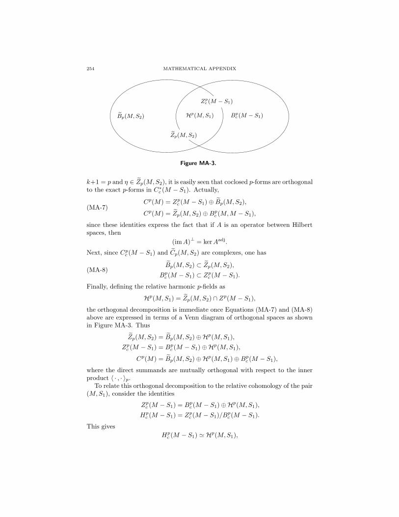
254 MATHEMATICAL APPENDIX
eBp(M, S2)
Zpc (M − S1)
Hp(M, S1) Bpc (M − S1)
eZp(M, S2)
Figure MA-3.
k+1 = p and η ∈ Zp(M,S2), it is easily seen that coclosed p-forms are orthogonalto the exact p-forms in C∗
c (M − S1). Actually,
Cp(M) = Zpc (M − S1)⊕ Bp(M,S2),
Cp(M) = Zp(M,S2)⊕Bpc (M,M − S1),(MA-7)
since these identities express the fact that if A is an operator between Hilbertspaces, then
(imA)⊥
= kerAadj.
Next, since Cpc (M − S1) and Cp(M,S2) are complexes, one has
Bp(M,S2) ⊂ Zp(M,S2),
Bpc (M − S1) ⊂ Zpc (M − S1).(MA-8)
Finally, defining the relative harmonic p-fields as
Hp(M,S1) = Zp(M,S2) ∩ Zp(M − S1),
the orthogonal decomposition is immediate once Equations (MA-7) and (MA-8)above are expressed in terms of a Venn diagram of orthogonal spaces as shownin Figure MA-3. Thus
Zp(M,S2) = Bp(M,S2)⊕Hp(M,S1),
Zpc (M − S1) = Bpc (M − S1)⊕Hp(M,S1),
Cp(M) = Bp(M,S2)⊕Hp(M,S1)⊕Bpc (M − S1),
where the direct summands are mutually orthogonal with respect to the innerproduct 〈 · , · 〉p.
To relate this orthogonal decomposition to the relative cohomology of the pair(M,S1), consider the identities
Zpc (M − S1) = Bpc (M − S1)⊕Hp(M,S1),
Hpc (M − S1) = Zpc (M − S1)/B
pc (M − S1).
This gives
Hpc (M − S1) ' Hp(M,S1),

MA-M. ORTHOGONAL DECOMPOSITIONS AND DUALITY THEOREMS 255
that is, in each de Rham cohomology class there is exactly one harmonic field. Amore concrete way of seeing this is to write the above orthogonal decompositionexplicitly in terms of differential forms and use the de Rham isomorphism. Thatis, any ω ∈ Cp(M) can be decomposed into three unique, mutually orthogonalfactors, say
ω = dν + δγ + χ,
where ν ∈ Cp−1c (M − S1), γ ∈ Cp+1(M,S2), and χ ∈ Hp(M,S2). Furthermore,
ω ∈ Zpc (M − S1) =⇒ ω = dν + χ,
ω ∈ Zp(M,S1) =⇒ ω = δγ + χ.
Thus if ω ∈ Zpc (M − S1) and zp ∈ Zp(M,S1), then∫
zp
ω =
∫
zp
dν +
∫
zp
χ =
∫
zp
χ, since
∫
zp
dν = 0.
Hence there is at least one harmonic field in each de Rham cohomology class.However it is easy to show that there cannot be more than one distinct harmonicfield in each de Rham cohomology class. Suppose that
ω1 − ω2 = dβ,
with β ∈ Cp−1c (M − S1), ω1 = dν1 + h1, and ω2 = dν2 + h2. Then
h1 − h2 = d(β − ν1 + ν2) ∈ Bpc (M − S1);
but by the orthogonal decomposition we have
h1 − h2 ∈ Hp(M,S1), Hp(M,S1) ⊥ Bpc (M − S1),
so h1 = h2 and there is necessarily exactly one harmonic field in each de Rhamcohomology class. Thus, explicitly, it has been shown that
Hpc (M − S1) ' Hp(M,S1);
hence
∞ > βp(M,S1) = βpc (M − S1) = dimHp(M,S1),
where the first equality results from the de Rham theorem. The preceding iso-morphism shows that the projection of ω on Hp(M,S1) is deduced from theperiods of ω on a basis of Hp(M,S1).
At this point we summarize the preceding discussion with a theorem.
Theorem (Orthogonal Decomposition of p-forms). Given M,S1, S2 as usualand
Hp(M,S1) = Zpc (M − S1) ∩ Zp(M,S2),
one has
(1) direct sum decompositions
Cp(M) = Bpc (M − S1)⊕Hp(M,S1)⊕ Bp(M,S2),
Zpc (M − S1) = Bpc (M − S1)⊕Hp(M,S1),
Zp(M,S2) = Bp(M,S2)⊕Hp(M,S1),

256 MATHEMATICAL APPENDIX
where the direct summands are mutually orthogonal with respect to theinner product 〈 · , · 〉p ; and
(2) a unique harmonic field in each de Rham cohomology class, that is, anisomorphism
Hp(M,S1) ' Hpc (M − S1),
so that
∞ > βp(M,S1) = βpc (M − S1) = dimHp(M,S1).
Having established the orthogonal decomposition theorem, it is useful to seehow duality theorems come about as a result of the Hodge star operator. As apreliminary, several formulas must be derived. Recall that if ω ∈ Cp(M) then
∗∗ω = (−1)p(n−p)ω, δpω = (−1)n(p+1)+1 ∗ d ∗ ω.Thus
∗δp = (−1)n(p+1)+1 ∗∗dn−p∗= (−1)n(p+1)+1+(p+1)(n−p−1) dn−p∗ ,∗dn−p = (−1)p(n−p) ∗dn−p ∗∗ = (−1)p(n−p)+n(p+1)+1δp∗ .
Cleaning up the exponents with modulo 2 arithmetic gives
∗δp = (−1)pdn−p∗ , ∗dn−p = −(−1)n−pδp∗ ,and hence
∗δn−p = (−1)n−p dp∗ , ∗dp = −(−1)pδn−p∗ .Next recall the identities
∗t = n∗, ∗n = t∗ .These six formulas will now be used to make some useful observations. Letλ ∈ Ck(M) and µ ∈ Cn−k(M), where ∗λ = µ. In this case
δkλ = 0 ⇐⇒ 0 = ∗δkλ = (−1)kdn−k ∗ λ = (−1)kdn−kµ,
dkλ = 0 ⇐⇒ 0 = ∗dkλ = −(−1)kδn−k ∗ λ = −(−1)kδn−pµ,
tλ = 0 ⇐⇒ 0 = ∗tλ = n ∗ λ = nµ,
nλ = 0 ⇐⇒ 0 = ∗nλ = t ∗ λ = tµ.
In other words, if λ, µ ∈ C∗(M) and ∗λ = µ, we have the equivalences
δλ = 0 ⇐⇒ dµ = 0,
tλ = 0 ⇐⇒ nµ = 0,
dλ = 0 ⇐⇒ δµ = 0,
nλ = 0 ⇐⇒ tµ = 0.
With a little reflection, the above four equivalences show that the Hodge staroperator induces the following isomorphisms, where 1 ≤ i ≤ 2, 1 ≤ k ≤ n:
Cp(M) ' Cn−p(M),
Ck(M,Si) ' Cn−kc (M − Si),Zk(M,Si) ' Zn−kc (M − Si),Bk(M,Si) ' Bn−kc (M − Si),Hk(M,Si) ' Hn−k
c (M − Si).

MA-M. ORTHOGONAL DECOMPOSITIONS AND DUALITY THEOREMS 257
What is particularly interesting is the following computation, where 1 ≤ i, j ≤ 2,i 6= j, 1 ≤ l ≤ n:
∗Hl(M,Si) = ∗(Zlc(M − Si) ∩ Zl(M,Sj)
)
= ∗(Zlc(M − Si)
)∩ ∗(Zl(M,Sj)
)
=(Zn−l(M,Si)
)∩(Zn−lc (M − Sj)
)
= Hn−l(M,Sj).
To interpret this result, notice that the derivation of the orthogonal decomposi-tion is still valid if S1 and S2 are interchanged everywhere. Hence, juxtaposingthe two orthogonal decompositions
Cp(M) = Bpc (M − S1)⊕Hp(M,S1)⊕ Bp(M,S2),
Cn−p(M) = Bn−p(M,S1)⊕Hn−p(M,S2)⊕Bn−pc (M − S2),
one sees that each term in these decompositions is related to the one directlyabove or below it by the Hodge star operator. Also, the star operation performedtwice maps Hp(M,S1) and Hn−p(M,S2) isomorphically back onto themselves,since in this case
(−1)p(n−p) ∗∗ = Identity.
HenceHp(M,S1) ' Hn−p(M,S2).
At this point it is useful to summarize the isomorphisms in (co)homologyderived in this chapter where coefficients are taken in R (of course) and M is anorientable, compact, n-dimensional Riemannian manifold with boundary where∂M = S1 ∪ S2 in the usual way.
Theorem.
Hk(M,S1) ' Hkc (M − S1) ' Hk(M,S1)
Hn−k(M,S2)
'
?
6
'Hn−kc (M − S2)'Hn−k(M,S2)
This theorem expresses the relative de Rham isomorphism (on the right),the representability of relative de Rham cohomology classes by harmonic fields(in the center), and the duality isomorphism induced on harmonic fields by theHodge star (on the left). For the inspiration behind this theorem see [Con54].
In order to let the orthogonal decomposition sink in, it is useful to rewrite itin terms of differential forms and then consider several concrete examples. Thusconsider the following theorem, which restates the orthogonal decompositiontheorem in a more palatable way:
Theorem. If M,S1, and S2 have their usual meaning and ω ∈ Cp(M), thenω has the unique representation
ω = dν + δγ + χ,

258 MATHEMATICAL APPENDIX
where
tν = 0, tχ = 0 on S1,
nγ = 0, nχ = 0 on S2,
dχ = 0, δχ = 0 in M and on ∂M .
Furthermore:
(1) The three factors are mutually orthogonal with respect to the inner product〈 · , · 〉p.
(2) If dω = 0 in M and tω = 0 on S1 one can take γ = 0.(3) If δω = 0 in M and nω = 0 on S2 then one can take ν = 0.
We illustrate the theorem with a couple of examples.
Example 7.13 The Hodge decomposition and 3-d vector analysis:n = 3, p = 1. In vector analysis it is customary to identify flux vector fields(arising from 2-forms) with vector fields arising from 1-forms by means of theHodge star operator. Keeping this in mind, the identifications established inExample 7.11 show that in the case of n = 3, p = 1 the theorem above canbe rewritten as follows. If M is an orientable, compact three-dimensional man-ifold with boundary embedded in R3, then any vector field V can be uniquelyexpressed as
V = gradϕ+ curlF + G,
where
ϕ = 0, n×G = 0 on S1,
F · n = 0, n ·G = 0 on S2,
curlG = 0, div G = 0 in M and on ∂M .
Furthermore:
(1) The three factors are mutually orthogonal with respect to the inner product
〈U ,V 〉1 =
∫
M
U · V dV.
(2) If curlV = 0 in M and n× V = 0 on S1, we may set F to zero;(3) If div V = 0 in M and V · n = 0 on S2, we may set ϕ to zero.
In practical problems it is customary to describe G through a (possibly mul-tivalued) scalar potential. The dimension of the space of harmonic vector fieldsthat satisfy the conditions imposed on G is β1(M − S1) = β2(M − S2). ˜
Example 7.14 The Hodge decomposition and 2-d vector analysis:n = 2, p = 1. Let M be an orientable compact 2-dimensional Riemannianmanifold with boundary where ∂M = S1 ∪ S2 in the usual way. Using theidentifications established in Example 7.12 one can rephrase the orthogonal de-composition theorem as follows. Any vector field V on M can be written as
V = gradφ+ curlψ + G,

MA-M. ORTHOGONAL DECOMPOSITIONS AND DUALITY THEOREMS 259
where
φ = 0, n×G = 0 on S1,
ψ = 0, G · n = 0 on S2,
curlG = 0, div G = 0 in M and on ∂M .
Furthermore:
(1) The three factors are mutually orthogonal with respect to the inner productgiven by the metric tensor in the usual way:
〈U ,V 〉1 =
∫
M
U · V dV.
(2) if curlV = 0 in M and n× V = 0 on S1 we may set ψ to zero.(3) if div V = 0 in M and V · n = 0 on S2 we may set φ to zero.
In practical problems G is invariably described in terms of a (possibly mul-tivalued) scalar potential or stream function. The dimension of the space ofharmonic vector fields which satisfy the conditions imposed on G is β1(−S1) =β1(M − S2). ˜
One final remark is appropriate. In the case of electrodynamics there is nopositive definite inner product on p-forms since the metric tensor is not positivedefinite. One can, however, define all of the spaces found in the orthogonaldecomposition and obtain a direct sum decomposition of Cp(M) even thoughthere is no positive definite inner product.
The committee which was set up in Rome for the unification of vectornotation did not have the slightest success, which was only to have beenexpected.
F. Klein, Elementary Mathematics from an Advanced Standpoint, 1925.


Bibliography
[AK98] V. I. Arnold and B. A. Khesin, Topological methods in hydrodynamics, Springer-
Verlag, New York, 1998.
[AL65] Holt Ashley and Marten Landahl, Aerodynamics of wings and bodies, Addison-
Wesley, Reading, MA, 1965, Section 2-7.[Alt55] M. Altman, A generalization of Newton’s method, Bulletin de l’academie Polonaise
des sciences III (1955), no. 4, 189–193, Cl.III.
[Arm83] M.A. Armstrong, Basic topology, Springer-Verlag, New York, 1983.
[Bat10] H. Bateman, The transformation of the electrodynamical equations, Proc. Lond.Math. Soc., II, vol. 8, 1910, pp. 223–264.
[BB69] N. Balabanian and T.A. Bickart, Electrical network theory, John Wiley, New York,
1969.
[BLG70] N. N. Balasubramanian, J. W. Lynn, and D. P. Sen Gupta, Differential forms onelectromagnetic networks, Butterworths, London, 1970.
[Bos81] A. Bossavit, On the numerical analysis of eddy-current problems, Computer Methods
in Applied Mechanics and Engineering 27 (1981), 303–318.[Bos82] A. Bossavit, On finite elements for the electricity equation, The Mathematics of Fi-
nite Elements and Applications IV (MAFELAP 81) (J.R. Whiteman, ed.), Academic
Press, 1982, pp. 85–91.
[Bos98] , Computational electromagnetism: Variational formulations, complementar-ity, edge elements, Academic Press, San Diego, 1998.
[Bra66] F.H. Branin, The algebraic-topological basis for network analogies and the vector cal-
culus, Proc. Symp. Generalised Networks, Microwave Research, Institute Symposium
Series, vol. 16, Polytechnic Institute of Brooklyn, April 1966, pp. 453–491.[Bra77] , The network concept as a unifying principle in engineering and physical
sciences, Problem Analysis in Science and Engineering (K. Husseyin F.H. Branin Jr.,
ed.), Academic Press, New York, 1977.[Bri93] Erik Brisson, Representing geometric structures in d dimensions: Topology and or-
der, Discrete and Computational Geometry 9 (1993), 387–426.
[Bro84] M. L. Brown, Scalar potentials in multiply connected regions, Int. J. Numer. Meth.
Eng. 20 (1984), 665–680.[BS90] Paul Bamberg and Shlomo Sternberg, A course in mathematics for students of
physics: 2, Cambridge U. Press, NY, 1990, Ch. 12.
[BT82] Raoul Bott and Loring W. Tu, Differential forms in algebraic topology, Springer-
Verlag, New York, 1982, pp. 40–42, 51, 234, 258, 240.[BV82] A. Bossavit and J.C. Verite, A mixed FEM-BIEM method to solve 3-d eddy-current
problems, IEEE Trans. Mag. MAG-18 (1982), no. 2, 431–435.
[BV83] , The ”TRIFOU” code: Solving the 3-d eddy-currents problem by using H as
state variable, IEEE Trans. Mag. MAG-19 (1983), no. 6, 2465–2470.[Cai61] S.S. Cairns, Introductory topology, The Ronald Press Company, 1961.
[Cam83] G. Cambrell, Upper and lower bounds, standard and complementary variational prin-
ciples of primal and dual kind, tonti diagrams for linear self-adjoint problems: Partsi and ii, Tech. report, Dept. of Elec. Eng. CADLab Seminars, McGill University, 1983.
261

262 BIBLIOGRAPHY
[CEG86] Thomas F. Coleman, Anders Edenbrandt, and John R. Gilbert, Predicting fill for
sparse orthogonal factorization, Journal of the Association for Computing Machinery
33 (1986), 517–532.[Chi68] G.E Ching, Topological concepts in networks; an application of homology theory to
network analysis, Proc. 11th. Midwest Conference on Circuit Theory, University of
Notre Dame, 1968, pp. 165–175.
[CK96] Paula Chammas and P. R. Kotiuga, Sparsity vis a vis Lanczos methods for discretehelicity functionals, Proceedings of the Third International Workshop on Electric
and Magnetic Fields (A. Nicolet and R. Belmans, eds.), 1996.
[Coh93] Henri Cohen, A course in computational algebraic number theory, Springer-Verlag,New York, 1993.
[Con54] P. E. Conner, The Green’s and Neumann’s problems for differential forms on Rie-
mannian manifolds, Proc. Nat. Acad. Sci. U.S.A. 40 (1954), 1151–1155.
[Con56] , The Neumann’s problem for differential forms on Riemannian manifolds,Mem. Amer. Math. Soc. 1956 (1956), no. 20, 56.
[Cou36] R. Courant, Differential and integral calculus, vol. II, Wiley-Interscience, New York,
1936.
[Cro78] F. H. Croom, Basic concepts of algebraic topology, Springer-Verlag, New York, 1978,Chaps. 2, 7.3, 4.5.
[Des81] Georges A. Deschamps, Electromagnetics and differential forms, IEEE Proc. 69
(1981), no. 6, 676–696.[Dod74] Jozef Dodziuk, Combinatorial and continuous Hodge theories, Bull. Amer. Math.
Soc. 80 (1974), no. 5, 1014–1016.
[Dod76] , Finite-difference approach to the Hodge theory of harmonic forms, Amer.
J. Math. 98 (1976), no. 1, 79–104.[dR31] Georges de Rham, Sur l’Analysis situs des varietes a n dimensions, Journ. de Math.
X (1931), no. II, 115–200.
[dR73] , Varietes differentiables. Formes, courants, formes harmoniques, troisieme
edition revue et augmentee, publications de l’institut de mathematique de l’universitede nancago, iii, actualites scientifiques et industrielles, no. 1222b ed., Hermann, Paris,
1973, First edition 1955. English edition published by Springer, 1984, is translation
of 1973 French edition.[DR91] E. Domınguez and J. Rubio, Computers in algebraic topology, The Mathematical
Heritage of C.F. Gauss (George M. Rassias, ed.), World Scientific Publ. Co., Singa-
pore, 1991, pp. 179–194.
[DS52] G. F. D. Duff and D. C. Spencer, Harmonic tensors on Riemannian manifolds withboundary, Ann. of Math. (2) 56 (1952), 128–156.
[Duf52] G. F. D. Duff, Differential forms in manifolds with boundary, Ann. of Math. (2) 56
(1952), 115–127.
[Dys72] F.J. Dyson, Missed opportunities, Bull. Amer. Math. Soc. 78 (1972), no. 5, 635–652.[ES52] Samuel Eilenberg and Norman Steenrod, Foundations of algebraic topology, Prince-
ton University Press, Princeton, New Jersey, 1952.
[Fla89] H. Flanders, Differential forms with applications to the physical sciences, Dover,
New York, 1989, pp. 79–81.[Fri55] K. O. Friedrichs, Differential forms on Riemannian manifolds, Comm. Pure Appl.
Math. 8 (1955), 551–590.
[Gau77] C. F. Gauss, Zur mathematischen Theorie der electodynamischen Wirkungen, WerkeV, Teubner, 1877, p. 605.
[GH81] Marvin J. Greenberg and John R. Harper, Algebraic topology, Benjamin/Cummings,
Reading, MA, 1981, P. 235, 63–66.
[Gib81] P.J. Giblin, Graphs, surfaces and homology: An introduction to algebraic topology,second ed., Chapman and Hall, London, 1981.
[GK95] P. W. Gross and P. R. Kotiuga, A challenge for magnetic scalar potential formula-
tions of 3-d eddy current problems: Multiply connected cuts in multiply connected
regions which necessarily leave the cut complement multiply connected, Electric and
BIBLIOGRAPHY 263
Magnetic Fields: From Numerical Models to Industrial Applications (New York)
(A. Nicolet and R. Belmans, eds.), Plenum, 1995, Proceedings of the Second Inter-
national Workshop on Electric and Magnetic Fields, pp. 1–20.[GK01a] , Data structures for geometric and topological aspects of finite element al-
gorithms, Progress In Electromagnetics Research (F. L. Teixeira, ed.), vol. PIER 32,
EMW Publishing, 2001, pp. 151–169.
[GK01b] , Topological constraints and computational complexity of finite element-basedalgorithms to make cuts for magnetic scalar potentials, Progress In Electromagnetics
Research (F. L. Teixeira, ed.), vol. PIER 32, EMW Publishing, 2001, pp. 207–245.
[Gol82] S.I. Goldberg, Curvature and homology, Dover Publications, New York, 1982.[GP74] Victor Guillemin and Alan Pollack, Differential topology, Prentice-Hall, Englewood
Cliffs, New Jersey, 1974, Page 21.
[GR65] Robert C. Gunning and Hugo Rossi, Analytic functions of several complex variables,
Prentice-Hall, Englewood Cliffs, N.J., 1965.[Har08] R. Hargraves, Integral forms and their connection with physical equations, Transac-
tions of the Cambridge Philosophical Society XXI (1908), 107–122.
[Her77] R. Hermann, Differential geometry and the calculus of variations, 2nd ed., Math.
Sci. Press, Brookline Mass., 1977.[Hip02] R. Hiptmair, Finite elements in computational electromagnetism, Acta Numerica
(2002), 237–339.
[Hir76] Morris Hirsch, Differential topology, GTM #33, Springer-Verlag, New York, 1976.[Hod52] W. V. D. Hodge, The theory and applications of harmonic integrals, 2d ed ed.,
Cambridge, at the University Press, 1952, The first edition, published in 1941 and
reissued in 1989, is subject to the criticism raised in [Wey43]. The second edition
benefited from the existence of a rigourous proof of the Hodge theorem.[HS85] C. S. Harrold and J. Simkin, Cutting multiply connected domains, IEEE Trans. Mag.
21 (1985), no. 6, 2495–2498.
[HY61] J.G. Hocking and G.S. Young, Topology, Addison-Wesley, 1961.
[Jac74] N. Jacobson, Basic Algebra I, W.H. Freeman and Company, San Francisco, 1974.[Jac80] , Basic Algebra II, W.H. Freeman and Company, San Francisco, 1980.
[KG90] P. R. Kotiuga and R. Giles, A topological invariant for the accessibility problem of
micromagnetics, J. Appl. Phys. 67 (1990), no. 9, 5347–5349.[KI59] K. Kondo and M. Iri, On the theory of trees, cotrees, multitrees, and multicotrees,
RAAG Memoirs 2 (1959), 220–261.
[Kle63] F. Klein, On Riemann’s theory of algebraic functions and their integrals, Dover, New
York, 1963.[Kod49] K. Kodaira, Harmonic fields in Riemannian manifolds (generalised potential theory),
Annals of Mathematics 50 (1949), 587–665.
[Koh72] J. J. Kohn, Differential complexes, Les Presses de l’Universite Montreal, 1972.
[Kot82] P. R. Kotiuga, Well-posed three dimensional magnetostatics formulations, Master’sthesis, McGill University, Montreal, August 1982.
[Kot84] , Hodge decompositions and computational electromagnetics, Ph.D. thesis,
McGill University, Montreal, 1984.
[Kot87] , On making cuts for magnetic scalar potentials in multiply connected regions,J. Appl. Phys. 61 (1987), no. 8, 3916–3918.
[Kot88] , Toward an algorithm to make cuts for magnetic scalar potentials in finite
element meshes, J. Appl. Phys. 64 (1988), no. 8, 3357–3359, Erratum: 64, (8), 4257,(1988).
[Kot89a] , An algorithm to make cuts for scalar potentials in tetrahedral meshes based
on the finite element method, IEEE Trans. Mag. 25 (1989), no. 5, 4129–4131.
[Kot89b] , Helicity functionals and metric invariance in three dimensions, IEEE Trans.Mag. 25 (1989), no. 4, 2813–2815.
[Kot89c] , Topological considerations in coupling scalar potentials to stream functions
describing surface currents, IEEE Trans. Mag. 25 (1989), no. 4, 2925–2927.

264 BIBLIOGRAPHY
[Kot91] , Essential arithmetic for evaluating three dimensional vector finite element
interpolation schemes, IEEE Trans. Mag. MAG-27 (1991), no. 6, 5208–5210.
[Kro59] G. Kron, Basic concepts of multidimensional space filters, AIEE Transactions 78(1959), no. Part I, 554–561.
[Lam32] Sir Horace Lamb, Hydrodynamics, Dover, New York, 1932, (1879).
[Lan70] Cornelius Lanczos, The variational principles of mechanics, University of Toronto
Press, Toronto, 1970.[LS68] L.H. Loomis and S. Sternberg, Advanced calculus, Addison-Wesley, Reading, Mas-
sachusetts, 1968.
[Lue69] D. G. Luenberger, Optimization by vector space methods, John Wiley, 1969.[Mac70] A.G.J. MacFarlane, Dynamical system models, George Harrap, London, 1970.
[Mas67] W. S. Massey, Algebraic topology: An introduction, GTM, vol. 56, Springer Verlag,
1967.
[Mas80] , Singular homology theory, GTM #70, Springer-Verlag, New York, 1980.[Max91] James Clerk Maxwell, A treatise on electricity and magnetism, third ed., Oxford
University Press, Clarendon, England, 1891, Republished Dover Publications, Inc.,
New York, 1954.
[MIK59] Y. Mizoo, M. Iri, and K. Kondo, On the torsion characteristics and the duality ofelectric, magnetic, and dielectric networks, RAAG Memoirs 2 (1959), 262–295.
[MN82] A. Milani and A. Negro, On the quasi-stationary Maxwell equations with monotone
characteristics in a multiply connected domain, Journal of Mathematical Analysisand Applications 88 (1982), 216–230.
[Mor66] C.B. Morrey, Multiple integrals in the calculus of variations, Springer-Verlag, Berlin,
1966.
[Mul78] Werner Muller, Analytic torsion and R-torsion of Riemannian manifolds, Advancesin Mathematics 28 (1978), 233–305.
[Mun84] James R. Munkres, Elements of algebraic topology, Addison-Wesley, Reading, MA,
1984, p. 377–380.
[Ned78] J. C. Nedelec, Computation of eddy currents on a surface in R3 by finite elementmethods, SIAM J. Numer. Anal. 15 (1978), no. 3, 580–594.
[Neu79] Lee Neuwirth, The theory of knots, Sci. Am. 240 (1979), no. 6, 110–124.
[PF84] J. Penman and J.R. Fraser, Unified approach to problems in electromagnetism, IEEProc. A 131 (1984), no. 1, 55–61.
[PF90] Alex Pothen and Chin-Ju Fan, Computing the block triangular form of a sparse
matrix, ACM Transactions on Mathematical Software 16 (1990), 303–324.
[Pin66] Tad Pinkerton, An algorithm for the automatic computation of integral homologygroups., Math. Algorithms 1 (1966), 27–44.
[Pos78] E. J. Post, The gaussian interpretation of ampere’s law, Journal of Mathematical
Physics 19 (1978), no. 1, 347.
[Pos84] , The metric dependence of four-dimensional formulations of electromag-netism, J. Math. Phys. 25 (1984), no. 3, 612–613.
[PP62] W. K. H. Panofsky and M. Phillips, Classical electricity and magnetism, Addison-
Wesley, Reading, MA, 1962, pp. 8–10, 20–23, 125–127.
[Rot55a] J. P. Roth, An application of algebraic topology to numerical analysis: On the exis-tence of a solution to the network problem, Proc. Nat. Acad. Sci. U. S. A. 41 (1955),
518–521.
[Rot55b] , The validity of Kron’s method of tearing, Proc. Nat. Acad. Sci. U. S. A. 41(1955), 599–600.
[Rot59] , An application of algebraic topology: Kron’s method of tearing, Quart. App.
Math. XVII (1959), no. 1, 1–24.
[Rot71] , Existence and uniqueness of solutions to electrical network problems viahomology sequences, Mathematical Aspects of Electrical Network Theory, SIAM-
AMS Proceedings III, 1971, pp. 113–118.
[Rot88] Joseph J. Rotman, An introduction to algebraic topology, Springer-Verlag, NY, 1988.

BIBLIOGRAPHY 265
[Sai94] I. Saitoh, Perturbed H-method without the Lagrange multiplier for three dimensional
nonlinear magnetostatic problems, IEEE Trans. Mag. 30 (1994), no. 6, 4302–4304.
[Sch95] G. Schwarz, Hodge decomposition: A method for solving boundary value problems,Lecture Notes in Mathematics, 1607, Springer-Verlag, 1995.
[SF73] Gilbert Strang and George Fix, An analysis of the finite element method, Wellesley-
Cambridge Press, Wellesley, MA, 1973.
[SF90] P.P. Silvester and R.L. Ferrari, Finite elements for electrical engineers, CambridgeU. Press, NY, 1990, 2nd Ed.
[Sle68] P. Slepian, Mathematical foundations of network analysis, Springer-Verlag, Berlin,
1968.[Sma72] S. Smale, On the mathematical foundations of electrical network theory, J. Differen-
tial Geom. 7 (1972), 193–210.
[Spa66] E. Spanier, Algebraic topology, Springer-Verlag, New York, 1966.
[Spi65] Michael Spivak, Calculus on manifolds. A modern approach to classical theorems ofadvanced calculus, W. A. Benjamin, Inc., New York-Amsterdam, 1965.
[Spi79] , A comprehensive introduction to differential geometry. Vol. I, second ed.,
Publish or Perish Inc., Wilmington, Del., 1979.
[Spr57] George Springer, Introduction to Riemann surfaces, Addison-Wesley, Reading, MA,1957, Section 5-8.
[SS54] Menahem Schiffer and Donald C. Spencer, Functionals of finite Riemann surfaces,
Princeton University Press, Princeton, N. J., 1954. MR 16,461g[SS70] L. M. Sibner and R. J. Sibner, A non-linear Hodge-de-Rham theorem, Acta Math.
125 (1970), 57–73.
[SS79] , Nonlinear Hodge theory: Applications, Adv. in Math. 31 (1979), no. 1, 1–15.
[SS81] , A sub-elliptic estimate for a class of invariantly defined elliptic systems,Pacific J. Math. 94 (1981), no. 2, 417–421.
[ST80] H. Seifert and W. Threlfall, A textbook on topology, Academic Press, 1980, Translated
by W. Heil from original 1934 German edition.
[Ste54] A. F. Stevenson, Note on the existence and determination of a vector potential,Quart. Appl. Math. 12 (1954), 194–198. MR 16,36a
[Sti93] John Stillwell, Classical topology and combinatorial group theory, second edition,
Springer-Verlag, NY, 1993, Ch. 3,4.[Str41] J. A. Stratton, Electromagnetic theory, McGraw-Hill, New York, 1941, pp. 227–228.
[Tar02] Timo Tarhasaari, Mathematical structures and computational electromagnetics,
Ph.D. thesis, Tampere University of Technology, Tampere, Finland, 2002.
[Tei01] F. L. Teixeira (ed.), Geometric methods for computational electromagnetics, ProgressIn Electromagnetis Research, no. 32, Cambridge, MA, EMW Publishing, 2001.
[Tho69] W. Thompson, On vortex motion, Transactions of the Royal Society of Edinburgh
XXV (1869), 217–280.
[Thu97] William P. Thurston, Three-dimensional geometry and topology, Princeton Univer-sity Press, Princeton, New Jersey, 1997.
[Ton68] Enzo Tonti, Gauge transformations and conservation laws, Atti Accad. Naz. Lincei
Rend. Cl. Sci. Fis. Mat. Natur. (8) XLV (1968), 293–300.
[Ton69] , Variational formulation of nonlinear differential equations. II, Acad. Roy.Belg. Bull. Cl. Sci. (5) 55 (1969), 262–278.
[Ton72a] , A mathematical model for physical theories. I, II, Atti Accad. Naz. Lincei
Rend. Cl. Sci. Fis. Mat. Natur. (8) 52 (1972), 175–181; ibid. (8) 52 (1972), 350–356.
[Ton72b] , On the mathematical structure of a large class of physical theories, Atti
Accad. Naz. Lincei Rend. Cl. Sci. Fis. Mat. Natur. (8) 52 (1972), 48–56.
[Ton77] , The reason of the analogies in physics, Problem Analysis in Science andEngineering (F. H. Branin Jr. and K. Husseyin, eds.), Academic Press, New York,
1977.
[Vai64] M. M. Vainberg, Variational methods for the study of nonlinear operators, Holden-
Day, San Francisco, 1964.

266 BIBLIOGRAPHY
[VB89] A. Vourdas and K. J. Binns, Magnetostatics with scalar potentials in multiply con-
nected regions, IEE Proc. A 136 (1989), no. 2, 49–54.
[Vic94] James W. Vick, Homology theory, second ed., Springer-Verlag, New York, 1994.[Wal57] A.H. Wallace, An introduction to algebraic topology, vol. 1, Pergamon Press, New
York, 1957.
[War71] F.W. Warner, Foundations of differentiable manifolds and lie groups, Scott, Fores-
man and Company, Glenview, Illinois, 1971.[Wei52] Andre Weil, Sur les theoremes de de Rham, Comment. Math. Helv. 26 (1952), 119–
145.
[Wey23] Hermann Weyl, Reparticion de corriente en una red conductora, Rev. Mat. Hisp.Amer. 5 (1923), 153–164.
[Wey43] , On Hodge’s theory of harmonic integrals, Ann. of Math. 44 (1943), 1–6.
[Whi37] Hassler Whitney, On matrices of integers and combinatorial topology, Duke Math.
Jnl. 3 (1937), no. 1, 35–45.[Whi50] , r-Dimensional integration in n-space, Proceedings of the International Con-
gress of Mathematicians, vol. 1, 1950.
[Whi57] , Geometric integration theory, Princeton University Press, Princeton, New
Jersey, 1957.[Yan70] Kentaro Yano, Integral formulas in Riemannian geometry, Marcel Dekker Inc., New
York, 1970, Pure and Applied Mathematics, No. 1.

Symbols in the list are sometimes also used temporarily for otherpurposes. . .
G. H. Hardy and E. M. Wright, An Introduction to the Theory of Numbers,5th ed.
Summary of Notation
Because the material in the book draws on a variety of fields, there are someresulting conflicts or ambiguities in the notation. In general, these ambiguitiescan be cleared up by context, and the authors have attempted to avoid situationswhere like notation overlaps in the same context. Some examples are:
(1) The symbol [ · , · ] can have three meanings: bilinear form, commutator, andhomotopy classes of maps.
(2) χ can have three meanings: Euler characteristic, stream function for a surfacecurrent, or a gauge function.
(3) π can be a permutation map or the ratio of circumference to diameter of acircle. In addition, πk signifies the kth homotopy group, while πk1 signifiesthe kth term in the lower central series of the fundamental group.
(4) R can be a resistance matrix, the de Rham map, or a region in R3.(5) Pullbacks and pushforwards of many varieties can be induced from a single
map. For example, an inclusion map i can induce maps denoted by i∗, i∗,i#, i[, ı, etc.
(6) The symbols ξ, λ, α, β, η, ρ, ν, and θ have meanings particular to Chapter 7(see Figure 7.4, page 211).
Other multiple uses of notation are noted below.
βp(R) pth Betti number = Rank Hp(R)δij Kronecker delta; 1 if i = j, 0 otherwiseδ Inner product space adjoint to the exterior derivativeδ Connecting homomorphism in a long exact sequence∂ Boundary operator∂T Coboundary operator.
∂ Boundary operator on dual mesh (related to ∂T )ε Dielectric permittivityζij jth 1-cocycle on dual mesh, indexed on 1-cells of DK: 1 ≤ i ≤
m1
267

268 SUMMARY OF NOTATION
η Wave impedanceθ Normalized angle of f : R −→ S1
θij θ discretized on nodes of unassembled meshλ Wavelengthλi Barycentric coordinates, 1 ≤ i ≤ 4µ Magnetic permeabilityπ Ratio of circumference to diameter of a circleπ Permutation mapπi ith homotopy group (but π0 distinguishes path components and
is not a group)ρ Volume electrical charge densityσ Electrical conductivityσs Surface electrical charge densityσp,i ith p-simplex in a triangulation of Rτe Dielectric relaxation time, τe = ε/σΦi ith magnetic fluxφ Electric scalar potentialχ Euler characteristicχ Stream function for surface current distributionχ Gauge functionχe, χm Electric and magnetic susceptibilitiesψ Magnetic scalar potentialψ+ (ψ−) Value of ψ on plus (minus) side of a cutω Radian frequencyΩ Subset of Rn
A Magnetic vector potentialB Magnetic flux density vectorBp(K;R) p-coboundary group of K with coefficients in module RBp(K;R) p-boundary group or K with coefficients in module RBp(K,S;R) Relative p-coboundary group of K (relative to S)Bp(K,S;R) Relative p-boundary group of K (relative to S)Bpc (M − S) Relative exact form defined via compact supports; S ⊂ ∂MBp(M,S1) Coexact p-forms in Cp(M,S1)c Speed of light in a vacuum, (ε0µ0)
−1/2
c Curve (or contour of integration)cp p-chaincp p-cochaincurl Curl operator
curl Adjoint to the curl operator in two dimensionsC Capacitance matrixC Constitutive law (see Figure 7.4)

SUMMARY OF NOTATION 269
Cijk Connection matrix, 1 ≤ i ≤ m3, 1 ≤ j ≤ 4, 1 ≤ k ≤ m0
Cip,jk Connection matrix of p-dimensional mesh
Cp(K;R) p-cochain group of K with coefficients in module RCp(K;R) p-chain group or K with coefficients in module RCp(K,S;R) Relative p-cochain group of K (relative to S)Cp(K,S;R) Relative p-chain group or K (relative to S)Cpc (M − S) Differential forms with compact support on M − S; S ⊂ ∂MCp(M,S1) p-forms in the complex defined by δ, the formal adjoint of d in
C∗c (M − S2)
d Coboundary operator; exterior derivatived Thickness of current-carrying sheetdiv Divergence operatordivS Divergence operator on a surfaceD Differential operatorD, δ Skin depthD Electric displacement fieldDK Dual cell complex of simplicial complex KE Electric field intensityEM Magnetic energyfp “Forcing function” associated with the pth cut (a vector with
entries fpi)f Frequencyf Generic functionf∗(µ) Pullback of µ by fF Rayleigh dissipation functionFp Free subgroup of pth homology groupF p Free subgroup of pth cohomology groupF Primary functionalF⊥ Secondary functional needed for convexityF s0 Number of FLOPs per CG iteration for node-based interpolation
of scalar Laplace equationF0 Number of FLOPs per CG iteration for node-based vector in-
terpolationF1 Number of FLOPs per CG iteration for edge-based vector inter-
polationF , G Spaces of vector fields with elements F and G, respectivelygrad Gradient operatorG Convex functionalH Magnetic field intensityHp(R; Z) pth cohomology group of R with coefficients in Z
Hp(R; Z) pth homology group of R, coefficients in Z

270 SUMMARY OF NOTATION
Hp(R, ∂R; Z) pth cohomology group of R relative to ∂R, coefficients in Z
Hp(R, ∂R; Z) pth homology group of R relative to ∂R, coefficients in Z
Hpc (M − S) Zpc (M − S)/Bpc (M − S); harmonic forms
Hp(M,S1) Zpc (M,S2) ∩ Zp(M − S1); harmonic fieldsi inclusion mapim Image of mapI Electrical currentIi ith currentIf ,Ip Free and prescribed lumped-parameter currentsInt ( · , · ) Oriented intersection numberI Intersection number matrixIp(m, l) Indicator function, 1 ≤ p ≤ β1(R), 1 ≤ m ≤ 4, 1 ≤ l ≤ m3
j Map inducing a third map in a long exact sequenceJ (Volumetric) current density vectorJav Average current density in effective depth of current sheetJ ij ∈ Z Nodal jumps on each element, 1 ≤ i ≤ m3, 1 ≤ j ≤ 4ker Kernel of mapK Surface current density vectorK Simplicial complexKkmn Stiffness matrix for kth element in meshK Global finite element stiffness matrixlmax “Characteristic length” of electromagnetic systemL Inductance matrixL LagrangianL2Λq(X) Space of square-integrable differential q-forms on manifold XLink( · , · ) Linking number of two curvesmp Number of p-simplexes in a triangulation of Rmp Number of p-cells in dual complexM MagnetizationM Manifoldnc, nv Number of prescribed currents and number of prescribed volt-
agesnp Number of p-simplexes in a triangulation of ∂Rn Normal vector to a codimension 1 surfacen
′ Normal to a two-dimensional manifold with boundary embeddedin R3
nz(A) Number of nonzero entries of a matrix AO(nα) Order nα
P Polarization densityP Poynting vectorP Period matrix

SUMMARY OF NOTATION 271
PJ Eddy current power dissipationQi ith chargeR Resistance matrixR de Rham map, R : L2Λq(X) → Cq(K) (K a triangulation of
X)R Region in R3, free of conduction currents
R Three-dimensional manifold with boundary, subset of R3
RS Surface resistivityS SurfaceS′, S′
ck Current-carrying surface after cuts for stream function havebeen removed, and the kth connected component of S ′
Sq qth cutS1 Unit circle, S1 = p ∈ C | |p| = 1T Kinetic energyT Vector potential for volumetric current distributionsTp Torsion subgroup of pth homology groupT p Torsion subgroup of pth cohomology groupT ∗ Cotangent spaceuk Nodal potential, 1 ≤ k ≤ m0
v vertexV VoltageVj Prescribed voltage, 1 ≤ i ≤ nvV Potential energywe Electric field energy densitywm Magnetic field energy densityW Whitney map W : Cq(K)→ L2Λq(X)We Electric field energyWm Magnetic field energyX Riemannian manifoldXs
0 # nonzero entries in stiffness matrix for node-based scalar in-terpolation
X0 # nonzero entries in stiffness matrix for node-based vector in-terpolation
X1 # nonzero entries in stiffness matrix for edge-based vector in-terpolation
z Complex conjugate of zzp p-cocyclezp p-cycleZp(K;R) p-cocycle group of K with coefficients in module RZp(K;R) p-cycle group or K with coefficients in module RZp(K,S;R) Relative p-cocycle group of K (relative to S)

272 SUMMARY OF NOTATION
Zp(K,S;R) Relative p-cycle group or K (relative to S)Zpc (M − S) Relative closed form defined via compact supports; S ⊂ ∂MZp(M,S1) Coclosed p-forms in Cp(M,S1)S+(−) Positive (negative) side of an orientable surface with respect to
a normal defined on the surfaceAc Set-theoretic complement of A[A,B] Homotopy classes of maps f : A→ B, i.e. π0(Map(A,B))[ · , · ] Homotopy classes of maps[ · , · ] Commutator[ · , · ] Bilinear pairing[ · ] Equivalence class of element ·∧ Exterior multiplication∗ Hodge star∩ Set-theoretic intersection∪ Set-theoretic union∪ Cup product

Examples and Tables
Example 1.1 Chains on a transformer 8
Example 1.2 Concentric spheres: Ω ⊂ R3, β2 6= 0 11
Example 1.3 Curves on a knotted tube: Ω ⊂ R3, β2 6= 0 11
Example 1.4 3-d solid with internal cavities: Ω ⊂ R3, H2(Ω) andH0(R
3 − Ω) of interest 11
Example 1.5 Curves on an orientable surface: Ω an orientable surface,H1(Ω) of interest 13
Example 1.6 Cohomology: Ω ⊂ R3 H2(Ω) is of interest 18
Example 1.7 Cohomology: Ω ⊂ R3,H0(Ω) is of interest 19
Example 1.8 Cohomology: Ω a 2-dimensional surface, H1(Ω) is of interest 20
Example 1.9 Cohomology: Ω ⊂ R3, H1(Ω) is of interest 22
Example 1.10 Fundamental group of the torus 26
Example 1.11 2-dimensional example of relative homology 33
Example 1.12 Torsion phenomena in relative homology 35
Example 1.13 Embedded surfaces and relative homology 39
Example 1.14 Electrostatics: Visualizing H1(Ω, S) in 3 dimensions 43
Example 1.15 Magnetostatics: Visualizing H2(Ω, S) in 3 dimensions 44
Example 2.1 The Lorentz gauge 55
Example 2.2 The Coulomb gauge 55
Table 2.1 Lumped parameters and cohomology groups 60
Example 2.3 Steady Current conduction in three dimensions: n = 3, p = 2 80
Example 2.4 Currents on conducting surfaces: n = 2, p = 1 85
Example 2.5 A billiard ball on a flat table as a nonholonomic system 90
Example 2.6 Ellipticity of the scalar Laplacian 96
Example 2.7 Ellipticity of the vector Laplacian 96
Example 2.8 Nonellipticity of the wave equation 96
273

274 EXAMPLES AND TABLES
Example 3.1 Poincare–Lefschetz dual of a submanifold 102
Example 3.2 Lefschetz duality in 3-d electrostatics: n = 3, p = 1 102
Example 3.3 Lefschetz duality in 3-d magnetostatics: n = 3, p = 2 103
Example 3.4 Duality and variational principles for magnetostatics 104
Example 3.5 Lefschetz duality and currents on orientable surfaces: n = 2,p = 1 107
Example 3.6 Lefschetz duality and stream functions on orientable surfaces:n = 2, p = 1 108
Example 3.7 Lefschetz duality and nonorientable surfaces 109
Example 4.1 Quadratic interpolation on 2-simplexes 126
Example 4.2 Lagrange polynomials on p-simplexes 127
Table 4.1 More on lumped parameters and cohomology 134
Example 4.3 Whitney form interpolation of the helicity functional 136
Table 6.1 Comparison of stiffness matrices in node- and edge-based finiteelement formulations 167
Table 7.1 Instances of the paradigm problem 186
Table 7.2 Cross-reference of paradigm problem instances to examples 186
Example 7.1 A convex function without a minimum 195
Example 7.2 Wedge multiplication in three dimensions 222
Example 7.3 Change of variables formula in two dimensions 224
Example 7.4 Change of variables formula for surface integrals in threedimensions 225
Example 7.5 Change of variables formula in three dimensions 225
Example 7.6 Exterior differentiation in one dimension 227
Example 7.7 Complex variables 227
Example 7.8 The classical version of Stokes’ theorem 228
Example 7.9 The divergence theorem in three dimensions 228
Example 7.10 Electrodynamics 229
Example 7.11 Vector analysis in 3-d orthogonal curvilinear coordinates 246
Example 7.12 Vector analysis in 2-d orthogonal curvilinear coordinates 247
Example 7.13 The Hodge decomposition and 3-d vector analysis: n = 3,p = 1 258
Example 7.14 The Hodge decomposition and 2-d vector analysis: n = 2,p = 1 258

Index
adjoint operator, 15, 16, 92, 93
admissible function, 122
admissible variation, 94, 189
Alexander duality theorem, 110–112, 118,
240
Ampere’s law, 25–27, 49, 104, 107, 113,117, 143, 160–161
approximation function, 126
atlas, 216
barrier, see also cut
barycentric coordinates, 124–126, 153, 171
Betti number, 11
for relative homology group, 33
Biot–Savart law, 114, 160, 165
black box model, 59
Bott, Raoul, 25
boundary, 11
operator, 10, 16, 30, 32, 42, 49, 132, 227
relative, 33
boundary value problem, 29, 99
branch cut, 15
branch voltage, 31
calculus
fundamental theorem, see also Stokes’
theorem on manifolds, 101, 227
multivariable, 7
variational, 149
cancellation error, 160
capacitance
and energy principles, 66
matrix, 66, 69, 70
capacitive
coenergy principle, 65
Cauchy–Riemann equations, 228
chain, 7
group with coefficients in R, 9
group with coefficients in Z, 9
group with coefficients in R, 9
homomorphism, 29
charge conservation, 20, 50
charge distribution, 103
chart, 216
Chrystal, G., 243
circuit parameters, 59, 128, 142
coboundary, 16
data structure, 137
operator, 10, 29, 30, 41, 42, 102, 129
cochain, 8, 41
group, 32
homomorphism, 30, 42, 231
maps, 231
cocycle
group, 16
coefficient group, 11, 16, 28, 38
coenergy principle, 63
cohomologous
absolute, 16
relative, 42
cohomology
de Rham, 131
relative, 41
cohomology group
absolute, 16
commutator, 26
subgroup, 26
compact support, 41
compatibility condition, 17, 99, 106, 191,
193
complex
cellular, 128, 131, 139, 174
chain, 28–30, 32
cochain, 28–31, 42, 132
extraction of, 131
simplicial, 43, 124, 127
simplicial data structure, 128
275

276 INDEX
conducting surface, 85
conjugate gradient method, 138, 167
constitutive law, 113
constitutive laws, 51
and energy principles, 73
cotangent bundle, 218
Coulomb gauge, 113
Cousin problem, 169
cup product, 100
curl, 20, 109
current, 103
on conducting surface, 85
steady conduction, 80
current power dissipation, 151, 155
current-carrying knot, 25, 114
cut, 14, 21, 25, 27, 108, 109, 112, 115, 117
cuts, 102, 159, 241
cuts algorithm, 161, 163
cycle, 11
relative, 33
cyclomatic number, 99, 111, 142
Davis, P. J., 181
de Rham isomorphism, 18, 73, 184, 201,233
relative, 42
differentiable manifold, 18, 43
disc with handles, 13
displacement current, 57, 112, 142, 160,185
dissipationless system, 89
divergence theorem, 228
duality theorem, 12, 99, 111
Alexander, see also Alexander duality
in electromagnetism, 101
Lefschetz, see also Lefschetz duality
Poincare, see also Poincare duality
Dyson, F.J., 215
eddy currents, 141, 142, 152
Eilenberg–MacLane space, 164, 240
electric
field, 46, 49, 160
flux density, 49, 64
vector potential, 64
electrical circuit theory, 24, 30, 128, 138
electrical flux, 103
electrical network, 31, 149
electromagnetic radiation, 58, 98
electromagnetic wave, 53, 59
electroquasistatics, 58–62
electrostatics, 19, 20, 43, 45, 67, 185, 214
elliptic equation, 96
elliptic operator, 252
embedded submanifold, 240, 241
energy principle
capacitive, 65
inductive, 72
equivalence class, 25, 117, 143, 216
equivalence relation, 11, 16, 42, 101
Euler characteristic, 138, 167, 177
Euler–Lagrange equation, 91, 94, 96, 147,154, 163, 168, 188
exterior algebra, 221, 222
exterior derivative, 10, 41, 226
exterior product, 100, 221
extraction, 172
Faraday’s law, 49, 147, 148, 151
finite element mesh, 124, 152
finite element method, 121, 122, 172, 183
flux density
electric, 19
magnetic, 46
force
electromotive, 64, 85, 106, 142
magnetomotive, 71, 74
form, 41
closed, 16, 18, 184
coclosed, 253
differential, 42, 43, 101, 131, 215, 217,218, 221, 227, 233
exact, 16
Fourier transform
and constitutive laws, 53
and retarded potentials, 61
fundamental group, see also homotopy
group, 128, 130, 178
fundamental theorem of calculus, 10
Galerkin form, 151, 165
gauge
Coulomb, 55, 58
function, 55
Lorentz, 55–58, 207
Gauss, 114
Gauss theorem, 101
Gauss’ law, 49, 50
Grassmann, 215
product, 221
Green’s function, 113
Green’s theorem, 101, 227
Hamilton, Sir William R., 183, 215
Hardy, G. H., 267
harmonic form, 252
harmonic function, 58, 166, 168
harmonic map equation, 165
hexahedral mesh, 128, 131
Hodge decomposition, 252

INDEX 277
Hodge star, 187, 244, 256
Hodge theory, 184
holonomic system, 89
homogeneous wave equation, 55
homologous, 11
homology
class, 18, 19, 22, 27, 38, 42, 163
generators, 39–41
homology group
absolute, 11, 34, 35, 37
relative, 33, 134, 143, 183
homotopy
class, 25–26, 163, 240
group, 25, 26
incidence matrix, 30, 31, 124, 132, 175, 178
inclusion map, 37
inductance
and energy principles, 72
matrix, 80, 97
inductive
coenergy principle, 74
energy principle, 72, 73
inhomogeneous boundary condition, 142
inner product, 93, 243, 244
integer coefficient group, 35
integral law, 21, 50, 51
interface condition, 190
interface conditions, 50, 51, 54, 190
intersection, 110
intersection matrix, 46, 75, 87, 103, 104,
107, 112, 117, 142, 143, 149
intersection pairing, 137
irrotational field, 23
isotropic media, 53, 56, 160
Kirchhoff current law, 31
Kirchhoff voltage law, 31, 58, 149
Klein, Felix, 259
Kron, Gabriel, 31, 215
Lagrange polynomial, 127
Laithwaite, E. R., 141
Laplace’s equation, 121, 122, 168
Laplace–Beltrami operator, 57, 252
Lefschetz duality theorem, 46, 60, 100,103, 104, 109, 110, 112, 117, 119, 139,
166, 238
and currents, 107
and nonorientable surfaces, 109
and stream functions, 108
in electrostatics, 102
in magnetostatics, 103
linear algebra, 124
linking number, 112, 114
long exact sequence
in cohomology, 42
in homology, 37
lumped parameter, 99
and cohomology, 60
magnetic
field, 49
flux density, 49, 70, 103, 104, 160
scalar potential, 113, 122, 128, 138, 141,143, 159, 172
magnetic flux, 103
magnetic scalar potential, 116
magnetoquasistatics, 58–62, 135
magnetostatics, 185, 214
manifold
differentiable, 216, 243
orientable, 100
Riemannian, 135, 243
Maxwell’s equations, 49–51, 160, 229
Maxwell, James Clerk, 49, 99, 111, 183
metric tensor, 185, 243
Mobius band, 232
Mobius band, 146
Morse, Marston, 7
Morse–Sard theorem, 241
multiply connected, 26, 28
multiply connected region, 160
multivalued function, 45, 46
nondegenerate bilinear pairing, 9, 43, 100
on cohomology, 100
nonorientable surface, 141, 145, 232
normalized angle, 169, 171
numerical analysis, 126, 135
Ohm’s law, 52, 59, 62, 160
orthogonal decomposition, 183, 192, 251,253
paradigm variational problem, 138, 183
perfect conductor, 103
period, 18
and circuit parameters, 59
relative, 42
periodicity constraint, 150
periphractic number, 13, 103
periphraxity, see also periphractic number
permittivity, 52
Poincare algorithm, 178
Poincare duality, 174
Poincare duality theorem, 100, 133
Poincare isomorphism, 27
Poincare map, 27
Poincare–Lefschetz dual of a submanifold,
102

278 INDEX
Poincare–Lefschetz duality theorem, 102,
134, 163
in magnetoquasistatics, 102Poincare-Lefschetz dual, 241
potential difference, 20, 103
potentials
for Maxwell’s equations, 53retarded, 61
Poynting theorem, 148, 151, 152
pullback, 163, 184, 219
quadratic interpolation, 126
quasistatics, 58
quotient group, 11, 32
Rayleigh dissipation function, 89, 91Riemann surface, 27
Riemannian structure, 185, 217, 243, 245
Ritz method, 122, 123
Russell, Bertrand, 47
scalar wave equation, 56, 59
scleronomic system, 91
simplex, 125, 128simply connected, 26
single-valued scalar potential, 22, 25, 71,
84, 117
skin depth, 47, 51, 53, 143solenoidal field, 58, 160, 228
solid angle, 112, 114
stereographic projection, 117, 118, 231
stiffness matrix, 123assembly, 127
Stokes’ theorem, 10, 15, 101, 102, 227, 228
stream function, 20, 21, 107, 109, 141, 143,
187
subcomplex, 30, 130, 131, 134, 172
symbol, 96
Tait, P. G., 49, 183
tangent vector, 217
tetrahedral mesh, 128, 130, 167
three-step procedure (homology genera-
tors), 38–40, 43, 44, 63, 74, 106, 187
time-varying, 58
Tonti diagram, 207, 211, 212
torsion subgroup, 35, 36, 112, 118, 119
transverse intersection, 112
trefoil knot, 24, 25, 27, 116, 160, 178
trial function, 123, 124, 126
tubular neighborhood, 112, 114
unassembled mesh, 169
universal coefficient theorem, 117, 118
variational principles
and cochain complex, 64, 72
electroquasistatics, 63
magnetoquasistatics, 70
vector
analysis, 7
vector analysis, 10–11, 15–18, 41, 246
wedge product, 221
Weizenbrock identity, 57
Weyl, Hermann, 159
Whitehead, A. N., 214
Wright, E. M., 267
Related Documents