The Role of Statistical Analysis in Groundwater … · The Role of Statistical Analysis in Groundwater Monitoring: A Florida Case Study James T. McClave, Sanford V. Berg and Cynthia

The Role of Statistical Analysis in Groundwater Monitoring;

A Florida Case Study

James T. McClave, Sanford V. Berg and Cynthia C. Hewitt

ABSTRACT

Most water quality monitoring programs ingnore, or at best paylip-service to, the fact that the water quality measurements are randomvariables, requiring probabilistic interpretation and statisticalestimation. We present a probabilistic definition of 'exceedance of aregulatory standard that recognizes the stochastic nature of waterquality monitoring. Interval estimates, rather than tests of hypotheses,are used to make inferences about the probability of exceedance. Theinterval estimates not only provide information about Type I and Type IIerror probabilities, but also measure the total amount of information inthe monitoring experiment. A Florida case study is utilized forillustration. -~.-

Keywords: water quality monitoring, exceedance probability, statisticalcompliance definitions, Type I and Type II errors, interval estimation.

The Role of Statistical Analysis in Groundwater Monitoring:A Florida Case Study

James T. McClave, Sanford V. Berg and Cynthia C. Hewitt l

Info Tech, Inc.Gainesville, Florida

'1.0 Introduction

Federal law mandates compliance of public drinking water systems with

primary standards, i.e., standards designed to protect public health. Examples

include limits on known carcinogens, such as asbestos, and toxic substances,

such as mercury. The Federal Safe Drinking Water Act also delineates secondary

standards adopted by the Environmental Protection Agency (EPA):

The.e secondary levels represent reasonable goals for drinking waterquality, but are not federally enforceable. Rather, they areintended as guidelines for the States. The States may establishhigher or lower levels as appropriate to their particularcircumstances dependent upon local conditions such as unavailabilityof alternate raw water resources or other compelling factors,provided that public health and welfare are adequately protected.(44 Fed. Reg. 42195.)

Health effects are generally not at issue at the levels specified by the

secondary standards; rather, they are intended primarily to protect the

aesthetic characteristics of drinking water. Twelve 'Pa-rameters, including-

color, corrosivity, and odor, are included. A complete list of the parameters

and the maximum levels for each are given in Table 1.

Florida has adopted the EPA secondary standards for community public

drinking water systems, as have seventeen other states. In adopting the

IDrs. McClave and Berg are Associate Professors in the Departments ofDecision and Information Sciences and in Economics, respectively, at theUniversity of Florida. Ms. Hewitt is a Senior Statistical Consultant at InfoTech, Inc. The support of the Florida Electric Coordinating Group isgratefully acknowledged. The views expressed herein are those of the authors,and do not necessarily represent those 'of affiliated or sponsoringorganizations.

1

TABLE 1

Florida Secondary Parameters and Standards

Parameter

ChlorideColorCopperCorrosivity

Foaming AgentsIronManganeseOdorpHSulfateTotal Dissolved Solids

Zinc

2

Standard (Maximum)

250mb/l15 color units1 mg/l-0.2 to +0.2(Langelier Index)0.5 mg/l0.3 mg/l0.05 mg/l3 (threshold odor number)6.5 (minimum allowable-no maximum)250 mg/l500 (may be greater if no other

standard is exceeded)5 mg/l

secondary standards for public drinking water on January 1, 1983, the Florida

Environmental Regulation Commission (ERC) also considered their applicability

to groundwater discharges, recognizing that they could ultimately impact upon

drinking water supplied by public authorities via individual wells. However,

the ERe decided that the application of secondary standards to groundwater

discharges might not always be appropriate. It chose to temporarily exempt

existing facilities discharging to gro~ndwater to enable further studies to be

undertaken; the Commission subsequently required existing dischargers to

-commence quarterly groundwater monitoring

... for the purpose of evaluating the environmental, social andeconomic benefits and costs, including but not necessarily limited tothose associated with the public health and aesthetic impacts on theenvironment, associated with requiring existing installations to meetsecondary standards.

Florida Administrative Code Rule 17-4.245(8)(b)

The ERe recognized an important difference in the application of secondary

standards to groundwater vis a vis drinking water: The Commission allowed for

adjustments due to natural background level of the secondary standards'

parameters when determining compliance of groundwater discharges with the

standards. Typically, facilities have three types of monitoring wells that are

- util ized to determine compl ianc:e with both primary and secondary standards :----

background wells are "upstream" from the groundwater discharge area,

intermediate wells are in the discharge area, and monitoring wells are

"downstream" from the discharge and on or close to the property line of the

facility. Of couI;se, the determination of what constitutes true "upstream" and

"downstream" locations is not an exact science, since in many cases the

direction of groundwater flow in the area of discharge is difficult to define

precisely. Nevertheless, the secondary parameters are compared to both the

standard and the background levels in determining compliance. Functionally,

3

noncompliance with secondary standards is declared only if both the standard

and naturally occurring background levels are exceeded.

The issue of clarifying an exceedance does not arise for standards

associated with non-naturally occurring substances. However, for secondary

standards, the underlying geological and hydrological features of the

particular geographic region can result in low quality groundwater. For

example, for much of Florida's groundwater salinity intrusion can result in

background levels of chloride that exceed EPA goals for drinking water.

A number of questions arise regarding the determination of noncompliance

by a discharging facility. Many questions are statistical in nature: How many.

samples are collected from each of the wells, and with what frequency? How

does one determine compliance ("nonexceedance") by comparing the monitoring

wells to both a fixed standard and a variable background? How does one control

the occurrence of "false positives" (declaring noncompliance when the facility

is in compliance) and "false negatives" (declaring compliance when the facility

is in noncompliance)? The EPA has recognized some of these issues in a

proposed groundwater monitoring rule 2 that explicitly addresses the statistical

issues arising in the analysis of groundwater data.

In the case of Florida, the ERC requirement that existing facilities

collect quarterly data on secondary parameters over at least a one year period

provides an unusual opportunity to address these issues. Florida, with its

combination of rapid growth and dependence on aesthetics to attract tourists,

provides a particularly relevant setting for such an analysis. The Florida

Electric Power Coordinating Group (FCG), an organization of 37 electric

utilities in Florida, commissioned an independent analysis of the data

2"Statistical Methods for Evaluating Ground-Water Monitoring Data FromHazardous Waste Facilities," Federal Register, Vol. 52, August 24, 1987.

4

collected by their members during this evaluation period. The final report 3 on

that analysis addresses the engineering, statistical, and economic issues of

applying secondary standards to Florida dischargers.

This study focuses on the statistical issues of groundwater monitoring.

Although the Florida analysis is utilized for illustration and to provide

specific examples, most of the issues apply not only to other groundwater

monitoring analyses, but to any determination of law in which a facility is

required to demonstrate that its discharge meets some fixed (or variable)

standard.

2.0 Exceedance Definition: Strict Liability vs. Probabilistic

The issue of defining noncompliance appears trivial: noncompliance occurs

when the level of a parameter exceeds the established standard. The EPA has

even coined the word "exceedance" to describe this event. However, the use of

exceedance and noncompliance synonymously is statistically problematic, since

it implies that the observed values of the parameter must never exceed the

(fixed) standard in order for a facility to be in compliance. Put in

probabilistic terms, if a facility is to be in compliance, then the probability

that the parameter exceeds the standard must equal zero. In recognition of the--

rigidity of such a standard, most regulatory personnel who must actually

enforce the standards look at one or more measurements that exceed the standard

in the context of other recent monitoring experience. The result is a

subjective, inconsistent (from regulator to regula~or) definition of

noncompliance.

3"Evaluation of the Impacts of Current Florida Secondary GroundwaterStandards on Electric Utilities;" Ch2M Hill, Info Tech, Inc., and Dr. SanfordBerg; February, 1987.

5

Because the parameter values observed at the wells are random variables

and the secondary standards are constants, the appropriate definition of an

"exceedance" is not obvious. For example, if an exceedance is said to occur

any time the obs~rved parameter value at a compliance well exceeds the

standard, or the background concentration, whichever is greater, then

exceedances of secondary standards are sure to occur with at least some non-

zero probability due to natural variations in groundwater characteristics.

Definitions which specify that any sample result exceeding the standard

constitutes a violation fall under the general heading of "strict liability"4

(Herricks 1985). Herricks et al. succinctly present the inherent scientific

principles that are violated by the strict liability definition:

. . where the results of the statistical analysis . .. bring intoques~ion the actual results of compliance monitoring (to say nothingof the initial process of standard setting), the very foundation ofstrict liability is threatened. Consider the following: If thestandard or permit limit is 1.0 mg/L, is an analytical result whichindicates a concentration of 1.01 mg/L a violation? Would aconcentration of 1.1 mg/L or 1.5 mg/L constitute a violation? Ifstrict liability is to be viable, the answer in each instance must beyes, even though prosecutorial discretion may dictate that no actualenforcement be taken. However, if there is a statistical probabilitythat even 1.5 mg/L is not a true violation, the doctrine of strictliability is meaningless. Strict liability can only function whenclearly defined limits are scientifically supported. The world mustbe black and white. Where statistical methods dem~nstrate that the·limitation, the standard, or the analytical result is not clearlydefined, the use of the strict liability doctrine would seemdoubtful.

Variability is intrinsic to measurement. A violation is asmuch--or more--a matter of statistics as it is of law. (p. 110)

Clearly, the doctrine of strict liability is not scientifically defen-

sible. A scientifically sound definition of exceedance must explicitly

recognize that the parameters are subject to random variation,attributable to

4As in Herricks et al., we define "strict liability" as follows: "Anysample result that exceeds an absolute numerical permit limitation or streamquality standard constitutes a violation." This should not be confused withthe term "strict liability" as it may be used in a legal sense.

6

a wide variety of sources. Berthouex (1974) recognizes three sources of

variability in reported water quality data: Process, Laboratory Analysis, and

Sampling. Although the extent of variability attributed to various sources is

debatable, the existence of variability is not. Regulations that are based on

scientifically valid definitions of exceedance can only acknowledge this

reality by specifying the probability with which the parameter must comply with

the standard, a probability that should be based on both sound scientific and

sound statistical research.

The use of statistical methods that recognize the stochastic (random)

nature of water ,quality monitoring and the probabilistic basis for the

resulting exceedance and water quality standards' definitions are receiving

increased attention in both the research literature and the regulatory

environment. Ward et ale (1985) address the stochastic nature of water quality

measurements and the need to interpret water quality standards in a

probabilistic context. Loftis et ale (1981, 1985) develop estimates and

confidence intervals for exceedance probabilities akin to those developed

herein. The EPA officially recognizes the importance of statistical sampling

methodology and the probabilistic assessment of exceedance (Federal Register,

August 1987) in the regulatory process.

For standards developed to protect aesthetic rather than health-related

values, a sensible definition of exceedance involves the central tendency of

the probability distribution of the parameter, rather than the upper extremes

of the distribution. If the mean or median of the parameter's distribution is

less than the standard, then we know that the standard will be met with a

probability of (approximately) .5. A standard set so that the probability of

compliance is .95 or .99 would be established at the 95th or 99th percentile of

the distribution and would assure that the standard would only be exceeded

7

about 5% or 1% of the time. While this might be desirable in some regulatory

frameworks, such requirements seem excessive (and often unattainable even in

the background) for secondary standards.

A probabilistic definition of secondary standard exceedance entails the

probabilities of three events:

1.

2.

3.

PCB > S)

P(C > S)

P(C >oB)

Probability that a Background measurement exceeds the

Standard

Probability that a Compliance measurement exceeds the

Standard

Probability that a Compliance measurement exceeds a

Background measurement

Exceedance of secondary standards might be defined in terms of these

probabilities! as follows:

1. If PCB > S) < .5, then an exceedance occurs if P(C > S) > .5. That is, if

the background median is less than the standard, then an exceedance occurs

if the compliance median exceeds the standard.

2. If PCB > S) ~ .5, then an exceedance o~curs if P(C > B) > .5. That is, if

the background median does exceed the standard, then an exceedance occurs

if the compliance median exceeds the background median.

The median rather than the mean is selected as the measure of central

tendency to identify an exceedance, because most of the secondary standard

water quality parameters have probability distributions that are significantly

skewed to the right. The lognormal distribution provides a credible model for

most of the parameters, and the geometric mean of a lognormal distribution is

5"Exceedance" for the secondary parameters pH and corrosivity involves alower standard (corrosivity has both a lower and upper standard). Determiningexceedance of a lower standard reverses the inequalities. That is, PCB < S),P(C < S), and P(C < B) are the relevant probabilities.

8

equal to the median. Thus, the above definition will utilize the geometric

rather than the arithmetic mean when the data are lognormal. For those

parameters that are analyzed under the assumption of normality (e.g., pH), the

median and the mean are equal. Thus, the use of the median offers robustness

(i.e., a degree of insensitiv~ty to the distribution of the data) to the

definition of exceedance. The two-part definition of exceedance is graphically

illustrated in Figure 1.

3.0 False Positives and False Negatives: Type I and Type II Errors

Adopting a probabilistic definition of exceedance does not solve all

problems connected with the determination of an exceedance. If the probability

distributions of the parameters could be estimated without error (as illus­

trated in Figure 1), then the determination of an exceedance could be

accomplished without further statistical analysis. However, the probability

distributions have to be estimated from sample data, which implies that the

medians, geometric means, arithmetic means and exceedance probabilities of the

background and compliance distributions will be estimated with uncertainty,

rather than with absolute precision.

In developing a statistical definition of exceedance that explicitly

acknowledges the uncertainty associated with the estimation of the probability

distributions of the parameters, two potential errors must be recognized: a

Type I error, or "false positive," is committed when an exceedance is declared,

but in fact no exceedance exists. A Type II error, or "false negative," occurs

when no exceedance is declared, but in fact one exists, where in each case the

"existence" of an exceedance is defined (precisely) according to the

probabilities given above. The objective, of course, is to minimize the

probabilities of making either Type I or Type II errors. However, some trade-

9

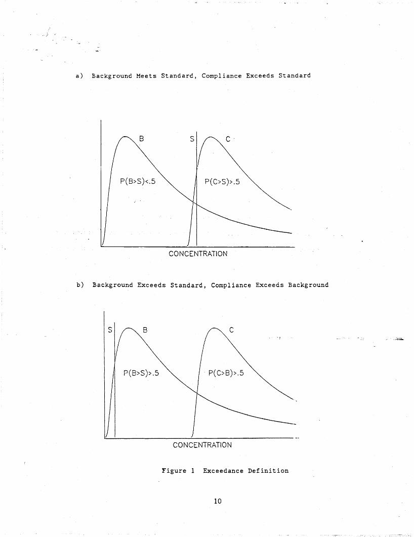
a) Background Meets Standard, Compliance Exceeds Standard

B

P(B>S)<.5

CONCENTRATION

b) Background Exceeds Standard, Compliance Exceeds Background

B

P(B>S».5

CONCENTRATION

Figure 1 Exceedance Definition

10

off will occur as long as we are working with sample information: for a given

sample size, the smaller the Type I error probability, the larger the Type II

error probability, and conversely.

Current groundwater monitoring data analysis places heavy reliance on

statistical tests of hypotheses, as evidenced by the EPA proposed methodology

(Federal Register, August 1987'). Although statistical tests permit the analyst

to specify, and therefore control, the Type I error probability, the value of

the Type II error probability generally remains unspecified, uncontrolled, and

often unmentioned in these analyses. The reason for this is rooted in the

methodology: the probability of a false negative result depends on the extent

of the exceedance, i.e., the amount by which the true median (if the median is

adopted as the relevant measure) exceeds the standard. The implication is that

the Type II error probability is not a single value, but instead a continuum of

values that decrease monotonically as the distance between the compliance

median and the standard increases.

Statistical tests are appealing because of their simplicity. The analyst

specifies the significance level of the test (the Type I error probability),

calculates the test statistic, and either concludes compliance or noncompliance

based on the result. The simplicity has a cost, however, since the result does.

not reflect anything about the potential Type II error, or about the

"information content" of the sample. Thus, tests depending on four

measurements look just like. those depending on four hundred measurements, and

those tests involving parameters whose standard errors are one order of

magnitude look just like those whose standard errors are ten orders of

magnitude.

Interval estimates for the probability of exceedance better reflect the

amount of information in the sample, without sacrificing the ability to make a

11

decision regarding noncompliance. For example, consider two 95% confidence

intervals for the probability 6 that a compliance measurement exceeds a fixed

standard: (.55, .65) and (.51, .91). Both would result in a conclusion that

the median exceeds the standard, since the lower confidence limit (LCL) exceeds

.5. Both conclusions would be made at the 5% (two-tailed) level of

significance, that is, the Type I error probability is .05 in each case.

However, the intervals provide something more: the first interval reflects

considerably more sample information than the second, so that inferences based

on the first interval reflect less uncertainty regarding the estimation of the

exceedance probability. Most analysts will therefore be more comfortable with

concluding that an exceedance has occurred based on the first, regardless of

the facts that the Type I error probabilities are identical and that both

intervals' lower bounds exceed .5. Consider a second pair of intervals, both

of which would result in a noncompliance conclusion: (.45, .55) and (.49,

.89). Clearly, the potential for a false negative in the second sample exceeds

that for the first. That is, although the intervals do not reveal the level of

Type II error probability, the need for more information in the second case is

evident.

As a further measure of the sample information, interval estimates can be ..

obtained for the. three exceedance probabilities using several different

confidence levels. For example, confidence levels of 68%, 95%, and 99.7%

correspond to Type I error probabilities of .32, .05, and .003,

6The interval could be constructed for the mean, median or any otherpercentile rather than for the exceedance probability with comparable results.The advantage of discussing the interval for exceedance probabilities is thatthe result is independent of both the parameter units and the specification ofthe percentile that constitutes exceedance.

12

respectively.' Thus, using the 68% confidence level, we are more likely to

declare an exceedance when in fact none exists (Type I error) than we are using

99.7% confidence. Conversely, we are more likely to miss an exceedance

(therefore incurring a Type II error) using the 99.7% confidence intervals than

we are using 68% confidence.

Recall that a secondary standard exceedance involves both a fixed standard

and a comparison of the compliance and background levels. Denoting the lower

confidence limit by LCL and the upper confidence limit by UCL, at any specified

confidence level, a secondary standard exceedance can be statistically defined

as follows:

1. If the UCL for PCB > S) is less than .5, an exceedance occurs if the LCL

for P(C > S) is greater than .5. That is, if at the specified confidence

level the background does not exceed the standard but the compliance does,

then an exceedance is said to have occurred.

2. If the LCL for PCB > S) is greater than .5, an exceedance occurs if the

LCL for P(C > B) is greater than .5. That is, if at the specified

confidence level the background exceeds the standard, then an exceedance

is said to have occurred only if the compliance exceeds the background.

3. If the LCL for PCB > S) is less than .5 and UCL is greater than .5 (a

"straddle"), then an exceedance occurs if either the LCL for P(C > S) or

the LCL for P(C > B) is greater than .5. That is, if at the specified

confidence level we are uncertain whether the background exceeds the

standard, then an exceedance is said to have occurred if the compliance

exceeds either the standard or the background.

'These (two-tailed) Type I error probabilities refer to the probabilitythat the confidence interval will not include the true probability. Becausethe definition of exceedance involves several of the probabilities, the Type Ierror probabilities do not equal the probability that an exceedance is declaredincorrectly. However, the two probabilities are proportional.

13

The three cases are illustrated in Figure 2. Although the statistical

definition requires some effort to understand and to implement, it is

imperative that the uncertainty with which the water quality parameter

distributions are estimated be recognized and utilized in defining an

exceedance. While probabilities of exceedance other than .5 could be used in

the definition, any definition should recognize the sampling variability

inherent in measurement of the water quality parameters. The presentation of

68%, 95%, and 99.7% confidence levels reveals the extent of uncertainty: the

width of the intervals reflects the information content of the sample, and the

degree of agreement regarding compliance is an indication of the sensitivity of

the result to the relative levels of Type I and Type II error probabilities.

4.0 Statistical Methodology

Once the probabilistic definition of noncompliance is adopted, the

statistical analysis of the water quality data should be conducted with the

primary objective of obtaining reliable confidence interval estimates of the

three exceedance probabilities discussed in the previous sections. Each of

the water quality parameters can be related to the factors of the experiment

using an analysis of variance model. The form of the model utilized in our

analysis of the Florida data is given by the following generic equation: 8

8The equation is shown without the multiplicative coefficients, orweights, for each of the factors on the right-hand-side of the equation. Thedegrees of freedom associated with each effect varies from parameter toparameter, making a generic version more efficient. The intent here is todisplay the factors themselves; estimates of the appropriate number ofcoefficients will, of course, be obtained from the data and will be utilized inthe estimation of geometric means and exceedance probabilities.

14

a) Background Less Than Standard; Compliance Exceeds Standard:UCL < .5 for PCB> S)) LCL > .5 for PCC ) S)

UCL!rOR a:

M~DIAN •

CONCENTR-"TION

b) Background and Compliance Exceed Standard:LCL > .5 for PCB > S») LCL > .5 for P(C > B)

Lf.~.f.Q~J~~'::.I?.l.~E;P'~~_? 0

CONCENTRATION

c) Background" Straddles" Standard;. Compl iance E~ceeds Either Backgroundor Standard:LCL < .5 < UCL for PCB > S)) LCL > .5 for PCC > S) or P(C > B)

!UCL:FOR BIMEDIAN

CONCENTRATION

Figure 2 Statistical Definition of Exceedance

15

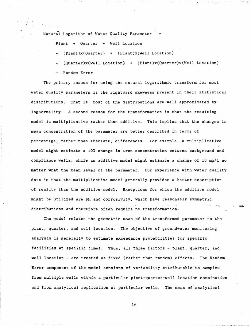
Natural Logarithm of Water Quality Parameter

Plant + Quarter + Well Location

+ (Plant)x(Quarter) + (Plant)x(Well Location)

+ (Quarter)x(Well Location) + (Plant)x(Quarter)x(Well Location)

+ Random Error

The primary reason for using the natural logarithmic transform for most

water quality parameters is the rightward skewness present in their statistical

distributions. That is, most of the distributions are well approximated by

lognormality. A second reason for the transformation is that the resulting

model is multiplicative rather than additive. This implies that the changes in

mean concentration of the parameter are better described in terms of

percentage, rather than absolute, differences. For example, a multiplicative

model might estimate a 10% change in iron concentration between background and

compliance wells, while an additive model might estimate a change of 10 mg/l no

matter what the mean level of the parameter. Our experience with water quality

data is that the multiplicative model generally provides a better description

of reality than the additive model. Exceptions for which the additive model

might be utilized are pH and corrosivity, which have reasonably symmetric

distributions and therefore often require no transformation.

The model relates the geometric mean of the transformed parameter to the

plant, quarter, and well location. The objective of groundwater monitoring

analysis is generally to estimate exceedance probabilities for specific

facilities at specific times. Thus, all three factors - plant, quarter, and

well location - are treated as fixed (rather than random) effects. The Random

Error component of the model consists of variability attributable to samples

from multiple wells within a particular plant-quarter-well location combination

and from analytical replication at particular wells. The mean of analytical

16

replicates was utilized for the analysis, so that well-to-well variation is the

primary source of error variability. Analytical replication was rare; the

model could have been expanded to recognize explicitly multiple sources of

variability had the replication been pervasive.

All terms in the model can be tested to determine whether model

simplification is possible. Of particular interest are the terms involving

Quarter, since they relate to the seasonality of the parameter. If no evidence

of seasonality is found, these terms can be dropped, and the determination of

exceedance made without regard to season. If the seasonal factor is important,

then exceedance determinations may also be seasonal, that is, plants may be

more likely to be noncompliant in specific quarters.

Several assumptions are necessary to assure the validity of the inferences

drawn from the analysis of variance models. The most relevant of these to

water quality analyses are that the (transformed) parameter is normally

distributed, and that the variance of the (transformed) parameter is constant

across the plant-quarter-well location combinations. Research and simulations

have shown that the validity of the model inferences is relatively insensitive

to departures from these assumptions (Electric Power Research Institute 1985).

Nevertheless, the distribution and variance of the (transformed) parameter

values should be analyzed to determine the degree of conformity with the

assumptions.

Another assumption that is necessary to the validity of inferences based

on the ANOVA model is the independence of the residuals. The assumption of

independence is most often violated when the data are time series, i.e., when

the data are observed at regular time intervals. Spatial correlation is

sometimes a concern, especially for sampling networks that are established at

fixed points. For the water quality data in the Florida study, both a spatial

17

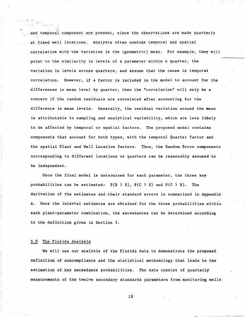
-and temporal component are present, since the observations are made quarterly

at fixed well locations. Analysts often confus~ temporal and spatial

correlation with the variation in the (geometric) mean. For example, they will

point to the similarity in levels of a parameter within a quarter, the

variation in levels across quarters, and assume that the cause is temporal

correlation. However, if a factor is included in the model to account for the

differences in mean level by quarter, then the "correlation" will only be a

concern if the random residuals are correlated after accounting for the

difference in mean levels. Generally, the residual variation around the mean

is attributable to sampling and analytical variability, which are less likely

to be affected by temporal or spatial factors. The proposed model contains

components that account for both types, with the temporal Quarter factor and

the spatial Plant and Well Location factors. Thus, the Random Error components

corresponding to different locations or quarters can be reasonably assumed to

be independent.

Once the final model is determined for each parameter, the three key

probabilities can be estimated: P(B > S), P(C > S) and P(C > B). The

derivation of the estimates and,their standard errors is summarized in Appendix

A. Once the interval estimates are obtained for the three probabilities withi~

each plant-parameter combination, the exceedances can be determined according

to the definition given in Section 3.

5.0 The Florida Analysis

We will use our analysis of the Florida data to demonstrate the proposed

definition of noncompliance and the statistical methodology that leads to the

estimation of key exceedance probabilities. The data consist of quarterly

measurements of the twelve secondary standards parameters from monitoring wells

18

"at twenty-eight power plant sites in Florida. The number of wells varies

considerably from plant to plant, and the onset of monitoring also differs.

The result is severe imbalance in the design, as shown in Table 2. Clearly,

many of the inferences will be based on extremely small sample sizes, and it is

important to utilize a statistical methodology that reflects this fact. Note

that some plants did not have designated compliance wells; in these cases the

intermediate wells were utilized to make inferences about compliance.

5.1 An Analysis of Iron

We will present the analysis for iron in some detail, and then su~arize

the results for the remainder of the parameters. The full analysis of variance

model for iron (log transform) is given in Table 3(a). Note that the levels of

statistical significance indicate that no term involving the Quarter effect is

significant, even at the .10 level. Most of the parameters failed to exhibit

significant seasonal variation in (geometric) mean level. Only Plant and

Location (of well) appear significant, and the (Plant)x(Location) interaction

is significant at the .0001 level. This indicates that statistically

significant differences exist between the geometric mean levels of iron among

the three well locations (background, intermediate, and compliance), but the

extent of the difference depends on the plant. In other words, any comparison

of background and compliance levels of iron should be conducted on a plant­

specific basis.

The final model for iron, involving only Plant and Location factors, is

given in Table 3(b). Note that the estimate of the model's standard deviation

(ROOT MSE) is 1.32. The implication in a logarithmic transform model is that

the random variability in iron measurements after accounting for plant and well

location is estimated by:

19

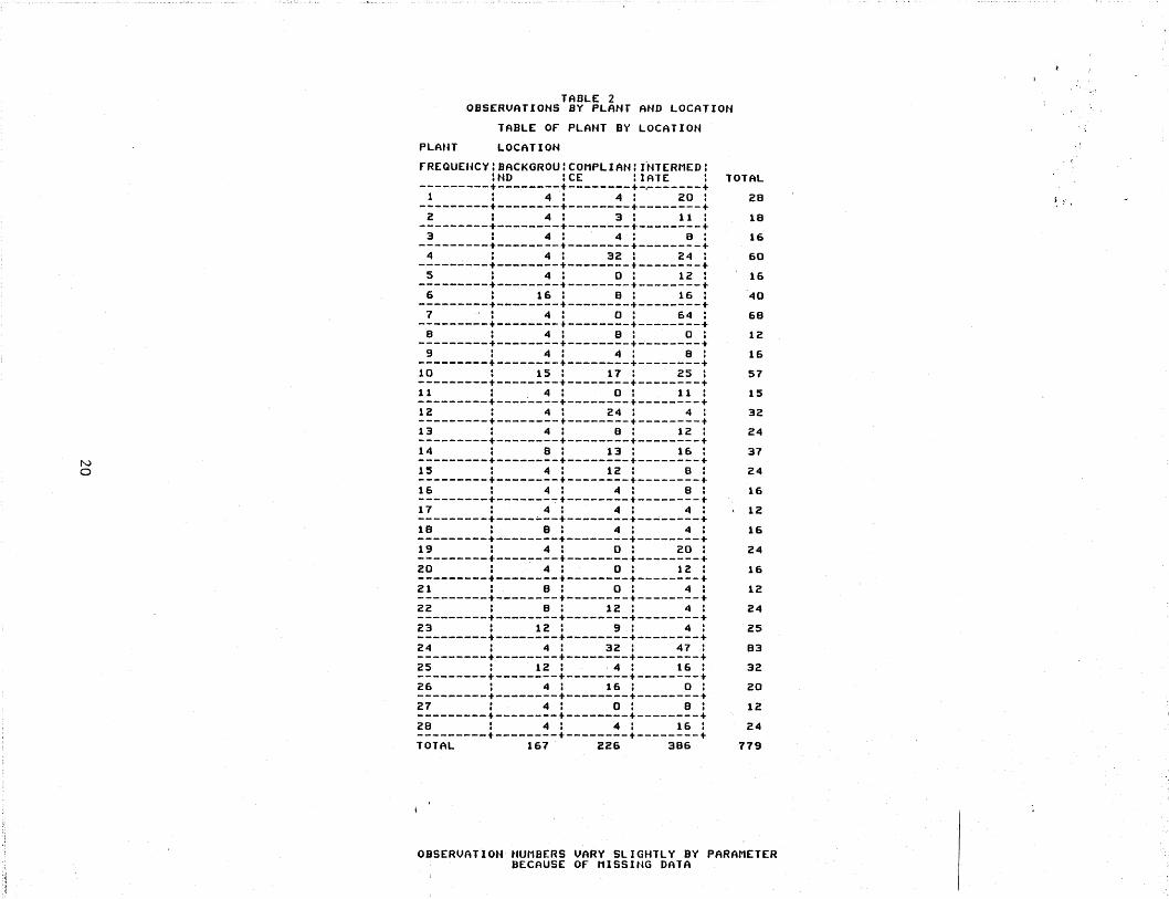
No

TABLE 2OBSERVATIONS BY PLANT AND LOCATION

TABLE Or PLANT BY LOCATION

PLAUT LOCATION

rREQUEUCY:BACKGROU:COMPLIAN:r'NTERMED:am : CE : lATE : TOTAL

---------t--------t--------t-~------t1 : 4 .: 4 : 20 : 28---------t--------t--------t--------t2 : 4 : 3 : 11: 18---------t--------t--------t--------t3 : 4 : 4 : 8 : 16---------t--------t--------t--------t4 : 4 : 32 : 24 : 60

-----~---t--------t--------t--------t5 : 4 : 0 : 12 : 16---------t--------t--------t--------t6 : 16 : 8 : 16 : 40---------t--------t--------t--------t1 : 4 : 0 : 64 : 68---------t--------+--------t--------t8 : 4 : 8 : 0 : 12---------t--------t--------t--------t9 : 4 : 4 : 8 : 16---------t--------t--------t--------t

10 : 15 : 11 : 25 : 57---------t--------*--------t--------t11 : 4 : 0 : 11: 15---------t----~---t--------t--------t12 : 4 : 24 : 4: 32---------t--------+--------t--------t13 : 4 : 8 : 12 : 24---------t--------t--------t--------t14 : 8 : 13 : 16 : 37---------t--------t--------t--------t15 : 4 : 12 : 8 : 24---------*--------t--------t-------_t16 : 4 : 4 : B : 16---------t--------t--------t--------t17 : 4 : 4 : 4 : 12---------t--------t--------t--------t18 : 8 : 4 : 4 : 16---------t--------t--------t--------t19 : 4 : 0 : 20 : 24---------t--------+--------t--------t20 : 4 : 0 : 12 : 16---------t--------t--------t--------t21 : B : 0 : 4 : 12---------t--------t--------t--------t22 : B : 12 : 4 : 24---------*--------t--------t--------t23 : 12 : 9 : 4 : 25---------*--------t--------t--------t24 : 4 : 32 : 47 : 83---------*--------t--------+--------t25 : 12 : ·4 : 16 : 32---------t--------t--------t--------t26 : 4 : 16 : 0 : 20---------t--------t--------t--------t27 : 4 : 0 : B : 12---------.--------t--------+--------t28 : 4 : 4 : 16 : 24---------t--------*--------t--------tTOTAL 161 226 386 119

OBSERVATIOH tlUMBERS VARY SLIGHTLY BY PARAMETERBECAUSE Or MISSING DATA

'.:- t

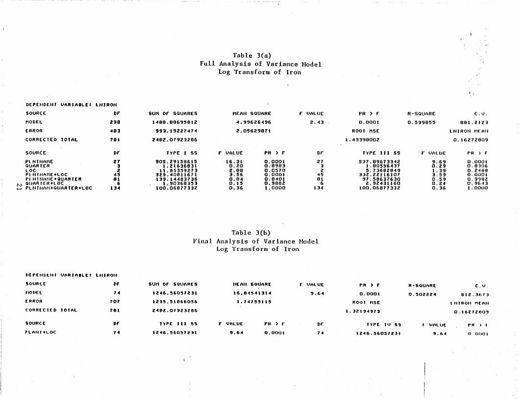
Table 3(a)Full Analysis of Variance Hodel

Log Transform of Iron

DEF>£ttDEtH VARIABL[I unROll

SOURCE Dr SUfi or SQUARES MEAH SQUARE r VALUE

MODEL 299 1.0499.88695812 4.99626496 2.43

ERROR 483 993.19227474 2.05629871

CORRECTED TOTAL 791 2492.07923286

SOURCE Dr TYPE I 55 r VALUE PR ) r DrPl.HTUAME 27 905.29158615 16.31 0.0001 27QUARTER 3 1.21636831 0.20 0.8983 3lOC 2 11.85359273 2.88 0.0570 2PlurUAHE+LOC 45 329.40811671 3.56 0.0001 45Pl U' tlMIE .QUARTER 91 139.14483736 0.84 0.8401 81

N QlJAIHER *L OC 6 1.90368353 0.15 0.9882 6...... PlffT'fnr,+QUARTER.LOC 134 100.06877332 0.36 1.0000 134

Table 3(b)Final Analysis of Variance Hodel

Log Transform of Iron

PR ) r0.0001

ROOT riSE

1.43398002

TYPE III 55

537.896733421.805964375.73682849

332.2211610797.58637630

2.92431160100.06877332

R-SQUARE

0.599855

r vnLUE

9.690.291. 393.590.590.240.36

, :

~ ;. ,

C.V.

881.2123

UU ROU tl£: AU

0.16272809

PR ) r

0.00010.83060.24880.00010.99820.96-131 • DOOO

1'[P£.tHJ£.tf, VARIABLEI LUIROll

SOURtE Itr SUM or SQUARES UEAII SQUnRE r VALUE PR ) r R-SQUARE C.V.tlOI'[L 74 12"'6.'6051231 16.8454'314 9.64 0.0001 0.502224 812.3673[RROR 701 1235.'1866056 1.7415'115 ROf) , MSE I teiROt. M[AU(ORREC 1[D 10tAL 781 24B2.01923286 1.3Z19491, 0.I621Z80'3

SOURCE Dr l'rPE III SS r VALUE: PH ) ,. Dr TYPE I'} SS r VALUE: f'R ) f

FLAtH .lOC 74 1246.56057231 9~64 0.0001 74 1246.56051231 9.6" 0,0001

a~til og ( ± 1 . 32) .27 to 3.74

The implication of this is that the random variability associated with these

measurements is such that one standard deviation stretches from 27% to 374% of

the geometric mean value at any given plant-well location. Most of the

parameters' model standard deviations are near 1.0, which (antilog) implies one

standard deviation variability from 37% to 272% of the geometric mean.

Sampling variability of an order of magnitude or more appears to be commonplace

among these parameters. This degree of variability emphasizes the need for a

statistical approach, and provides hard evidence against the utilization of

strict liability for noncompliance decision-making.

The residual analysis for the iron model is best summarized by a series of

graphics. Figure 3 shows a frequency distribution plot for all the residuals;

note that the distribution appears to be relatively symmetric, implying that

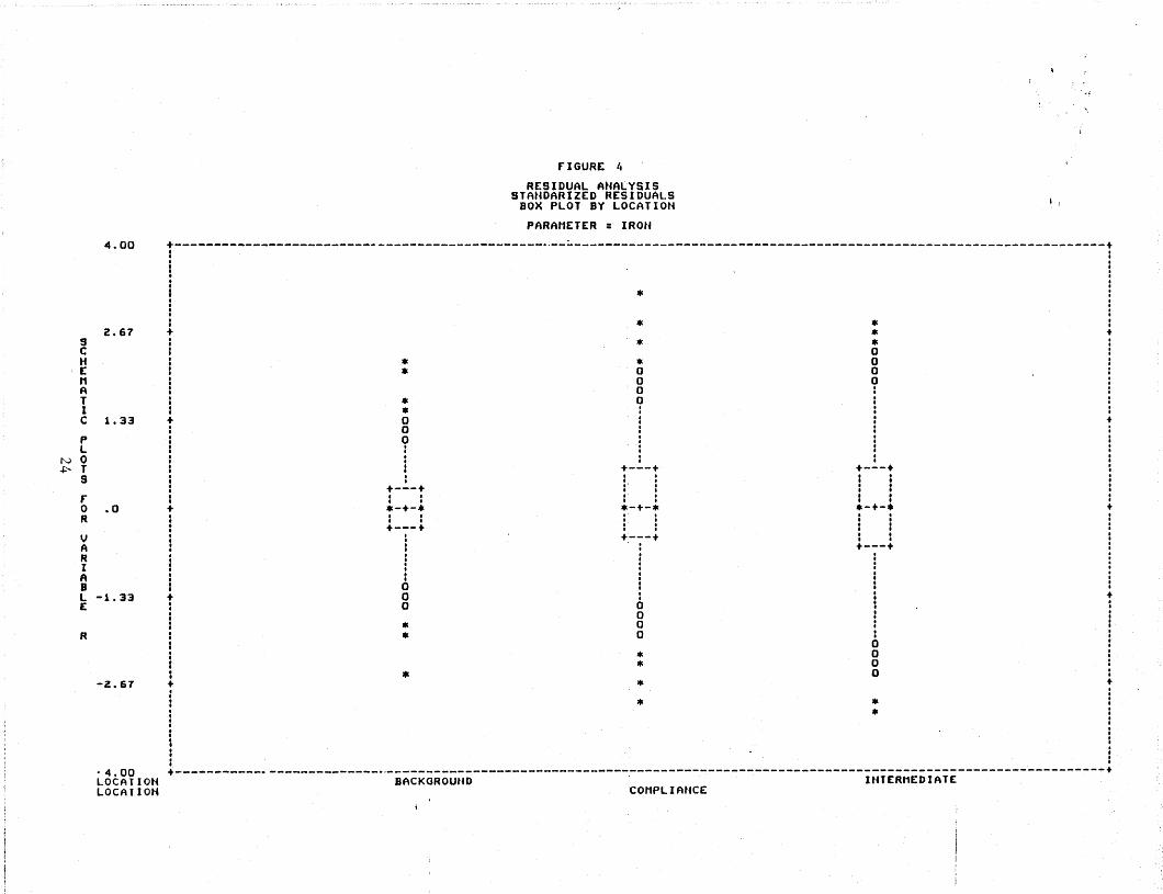
the log-normality assumption is reasonable. Figure 4 is a "box plot" of the

residuals by well location. Box plots are useful for examining variability,

since the two narrow ends of the box (rectangle) represent the 25th and 75th

percentiles of the distribution. Extreme observations are denoted by the

symbol '*' on the plot. Although the box plots indicate differences in sample

variability among well locations, no extreme differences are noted. The most

extreme difference occurs between background and intermediate wells, where the

ratio of variance is approximately 3 to 1. The EPRI study [1985] on robustness

indicated a 6 to 1 ratio in variances could be tolerated before statistical

inferences are significantly affected. Box plots of residuals by plant also

reveal relative homogeneity.

Finally, the residual variances for the 28 plants were calculated, and

their log transforms were regressed on plant characteristics, like setting,

type of fuel used, salinity, etc. The result is shown in Table 4. Note that

22

fIGURE 3

RESIDUAL AUALYSISSTANPARIZED RESID~ALS

fREQUENCY DISTRIBUTION

PARAMETER: IRON

PERCENTAGE BAR CHARTPERCENTAGE

+

+

+

+···I·I

+II·!+···l

+····I·

···!+

+·I···I+···l

.*********•••**••• *•••••*•••***.**.*****••****.****•• **••*.*.*****.***••****••*....... * .****••••• *"''''.*•••*. *"'*.'"••**'" .****••*** .**.*•••• '" ••••*•••*. •.... *.

•••** ••*** ********** .**** .********* *.*** ********"'. .***. ****.*.*.. *•••* ***.****** *.*** .**.****.* .**.. .**.***••* •••** **••**••** ••••* **.**.*•• * •••** .*••****.* ••**. *****.**** ••*** .*.** .****••••• • •• ** .**.* .**•••••** ••*** **••* *•••*••••* **.** ****. ******••*. ***.. • •• ** *.*.*

***** ***.* ••••* ••*.. *.*.**••** **••* .*••* **... ****•

••••* **••* .*... **.** **.** **••*••••* ••••• **.** ••••* ***** *.*.*••••• ••••• ** ••* .**.. • ••** *••**••••• *••** .*••* ***** .*... *•••*••••• ..*.* •••** ••*.. *.*.* ••••*••••• *.*** *.*.. • ••** *.*** **.** *****

+ *.*** **••* ***** .**** ***** .*.** **•••: •••** .•**** *.*** ***** **.** ***** .*.**: ••*** **••* ***** ••*** *.*** *.*** *****: ***** ***** ***** .**** ••*.. ***.* ***** *••** **.**+ ••*.* *••*. ..**. ***** .**** ***** *.*** **.** *.***: ••*** ••*** *.... **.** **.** ***** ****. **••* .****: ***** ***** ••••* *.*** ***.* *.*** ***** ** ••* .**** ***.* *.*.*: ***** ••••* •••** **.*. ****. .**** ***** ****. *.*** ••*** ****. ***** *.*.*--------------------------------_.----~--_.-------------------------------------------------------------------------------------3.0 -2.5 -2.0 -1.5 -1.0 -O.~ 0.0 O.S 1.0 1.~ 2.0 2.~ 3.0

RESIDUAL MIDPOINT

26

24

22

20

N 18W

16

14

12

10

8

6

4

2

',;"

r IGUR£ 4

RESIDUAL ANALYSISSTANDARIZED RESIDUALS

BOX PLOT BY LOCATION

PARAMETER = IRON" '

.0

1. 33

COMPLIANCE

+··:·,:,··,·I..**

oooo

**

••*

+----------------------------------------------_.,--~--------------------------------------------------------------------+! :: :: !! * :: :· :: * * :t *: ~I 0:: * * 0 ",': * 0 0

! g? 1: * 0 : :: * : : :+ 0 :,' : ..: 0 :,: 9 : : :,': . : :• • I • •

: : +-~-+ +-~-+ :• I • • •: +-~-+ :' : :: : : : . : : :+ *-+-. *-+-. .-+-. ..· . . . . .· . . . : .: +-:--+ : : :• , +---+ I I: : : +- -+, , ,J : :: : .i a i+,0:100

: 0I * 0, * 0i,:·:+,:·,•···I·I··: .+----------_.-------------_.._-------------------------------------------------------------------------------------------+BACKGROUND INTERMEDIATE

·4.00LOCATIOULOCATIOU

R

4.00

l.67

-Z.67

9CH[MAT1C

PL

N 0.f;-- T

S

roR

VARIABL -1. 33[

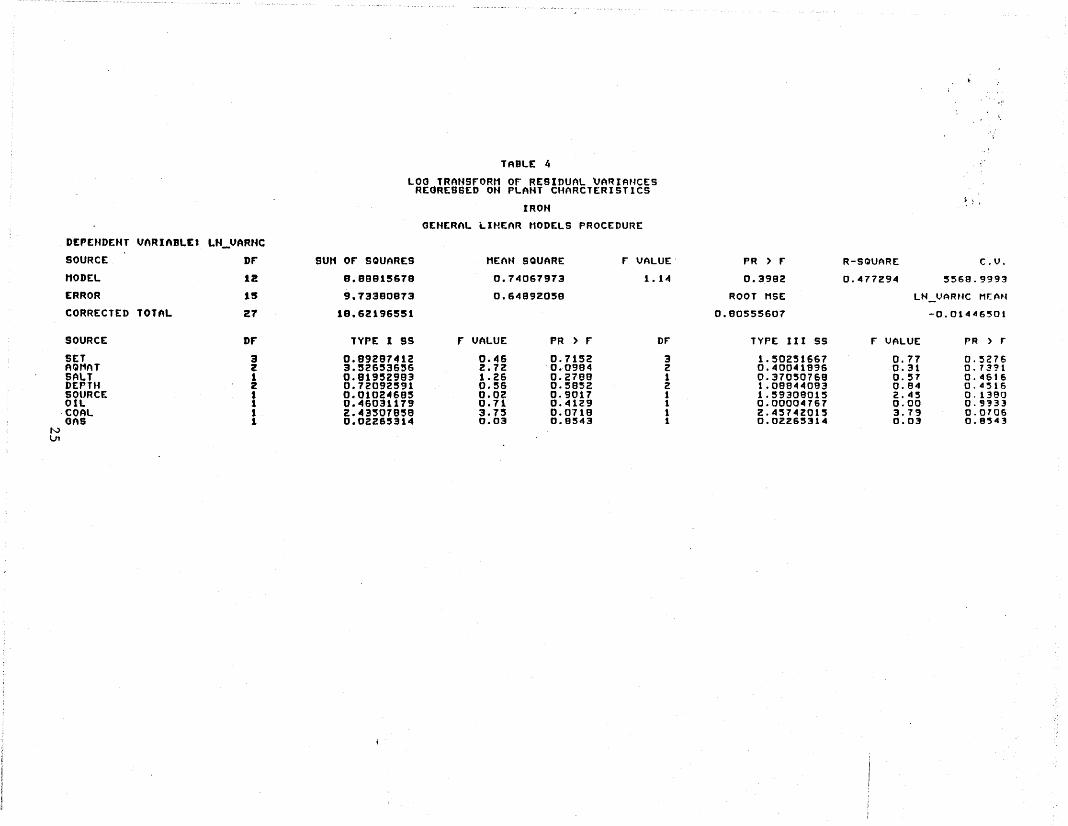
TABLE 4

LOG TRANsrORM or RE8IOUAL UARIANCESREGRESSED ON PLAHT CHARCTERISTICS

IROH

GENERAL LIHEAR MODELS PROCEDURE

r VALUE PR ) r

0.77 0.52760.31 O.73·H0.57 0.46160.B4 0.45162.45 0.13800.00 0.93333.79 0.07060.03 0.8543

DEPENDENT VARIABLE' LH_VARHC

SOURCE DF" SUN OF" SQUARES MEAN SQUARE

MODEL 12 9.99815&78 0.740&7973

ERROR 15 9.13380973 0.&4892058

CORRECTED TOTAL 21 19.62196551

SOURCE DF" TYPE I SS F" VALUE fR ) r

SET 3 0.99297412 0.46 0.7152AQt1AT 2 3.~2653656 2.72 0.0994SALT 1 0.91952993 1.26 0.2789DEPTH 2 0.72092591 0.56 0.5952SOUF~CE t 0.0102<4685 0.02 0.9017OIL 1 0.46031179 0.71 0.4129COAL t 2.43507959 3.75 0.0719GAS 1 0.02265314 0.03 0.9:543

NV1

r VALUE'

1.14

Dr32121111

PR ) r0.3992

ROOT MSE

0.90555607

TYPE III 5S

1.502516670.400419960.370507681.089440831.593090150.000047672.457420150.02265314

R-SQUARE

0.477294

C.V.

5569.9993

U~_VAR"C MtAN

-0.01446501

the overall"significance of the model is .2455, indicating no statistically

significant correlation between residual variance and plant characteristics.

This result lends further support to the assumption that the random component

of the model has constant variance across plants and well locations.

Satisfied that the model adequately describes the relationship between

iron concentration and the plant-well location, and that the assumptions neces-

sary to make inferences from the model are reasonable, the model is used to

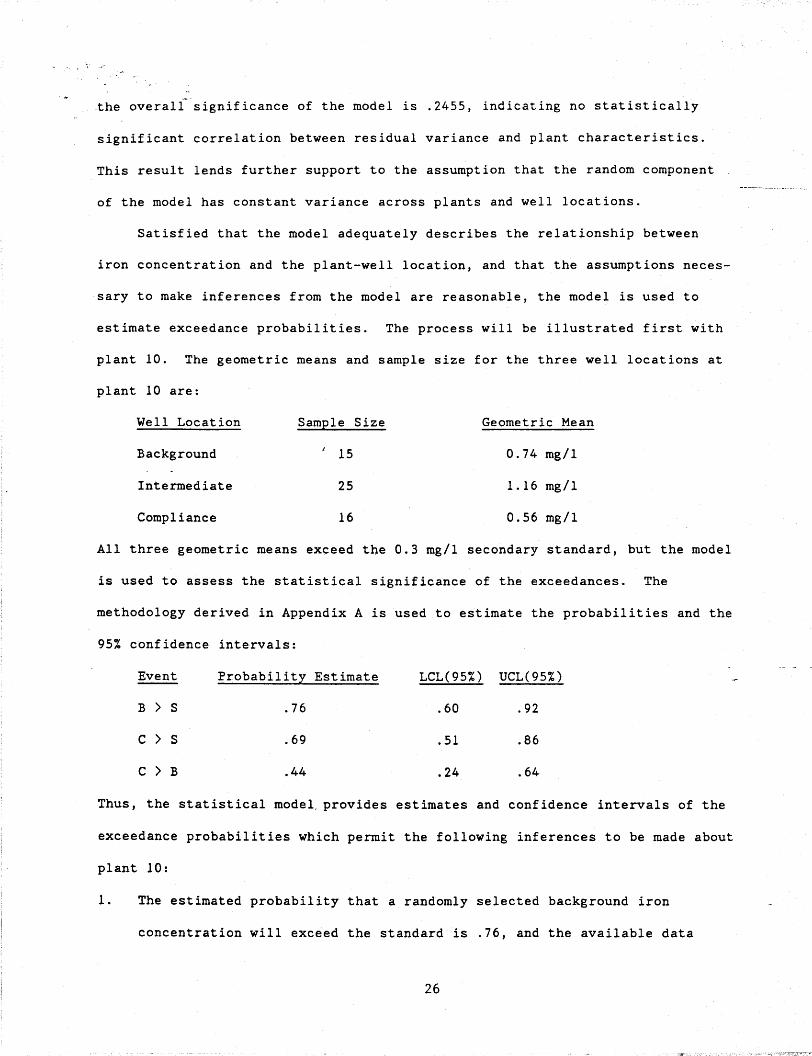
estimate exceedance probabilities. The process will be illustrated first with

plant 10. The geometric means and sample size for the three well locations at

plant 10 are:

Well Location

Background

Intermediate

Compliance

Sample Size

I 15

25

16

Geometric Mean

0.74 mg/l

1.16 mg/l

0.56 mg/l

All three geometric means exceed the 0.3 mg/l secondary standard, but the model

is used to assess the statistical significance of the exceedances. The

methodology derived in Appendix A is used to estimate the probabilities and the

95% confidence intervals:

Event

B > S

C > S

C > B

Probability Estimate

.76

.69

.44

LCL(95%) UCL(95%)

.60 .92

.51 .86

.24 .64

Thus, the statistical model, provides estimates and confidence intervals of the

exceedance probabilities which permit the following inferences to be made about

plant 10:

1. The estimated probability that a randomly selected background iron

concentration will exceed the standard is .76, and the available data

26

-indicate that we can be 95% confident that the true probability is between

.60 and .92.

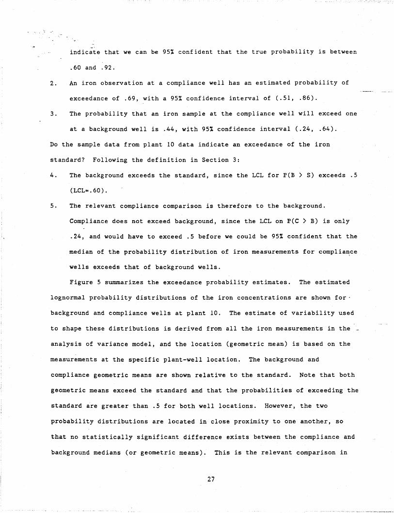
2. An iron observation at a compliance well has an estimated probability of

exceedance of .69, with a 95% confidence interval of (.51, .86).

3. The probability that an iron sample at the compliance well will exceed one

at a background well is .44, with 95% confidence interval (.24, .64).

Do the sample data from plant 10 data indicate an exceedance of the iron

standard? Following the definition in Section 3:

4. The background exceeds the standard, since the LCL for P(B > S) exceeds .5

(LCL=.60).

5. The relevant compliance comparison is therefore to the background.

Compliance does not exceed background, since the LCL on P(C > B) is only

.24, and would have to exceed .5 before we could be 95% confident that the

median of the probability distribution of iron measurements for complia~ce

wells exceeds that of background wells.

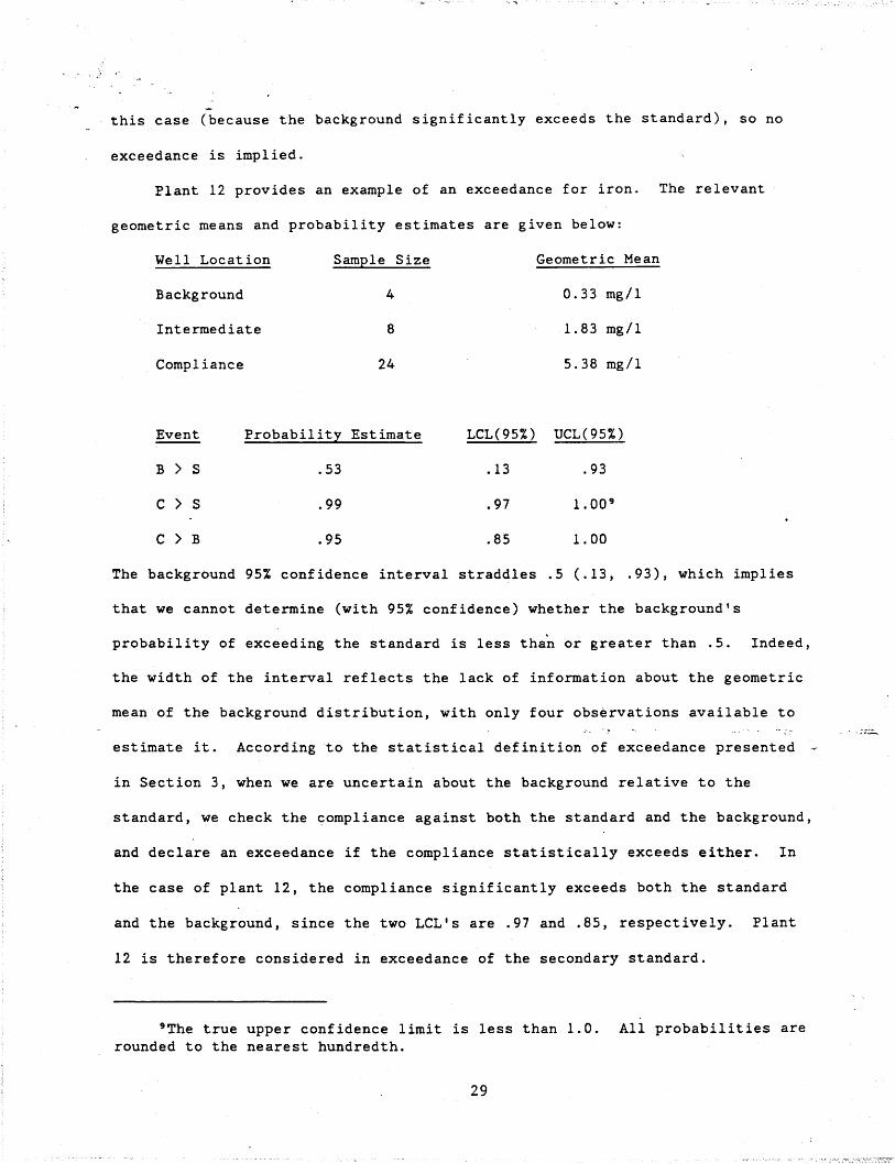
Figure 5 summarizes the exceedance probability estimates. The estimated

lognormal probability distributions of the iron concentrations are shown for'

background and compliance wells at plant 10. The estimate of variability used

to shape these distributions is derived from all the iron measurements in the ._

analysis of variance model, and the location (geometric mean) is based on the

measurements at the specific plant-well location. The background and

compliance geometric means are shown relative to the standard. Note that both

geometric means exceed the standard and that the probabilities of exceeding the

standard are greater than .5 for both well locations. However, the two

probability distributions are located in close proximity to one another, so

that no statistically significant difference exists between the compliance and

background medians (or geometric means). This is the relevant comparison in

27

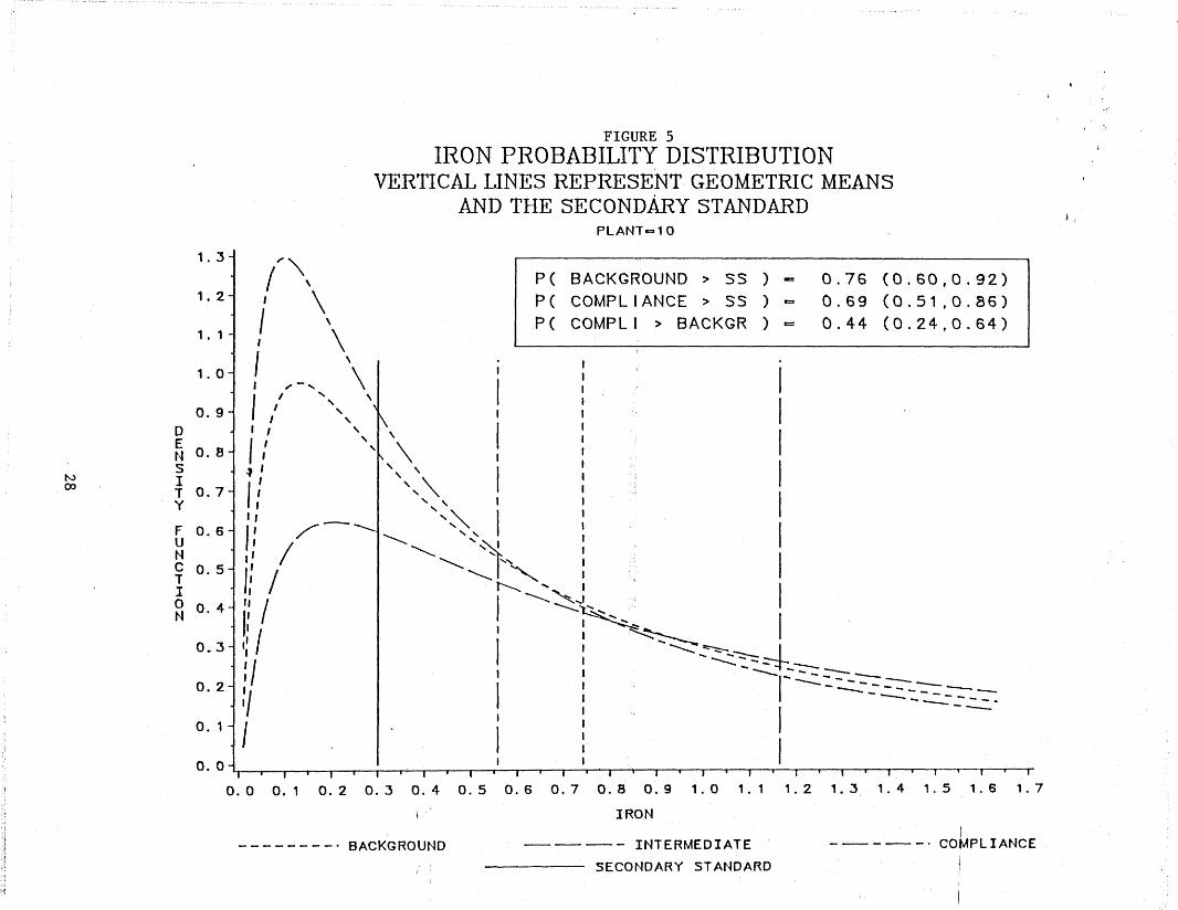
FIGURE 5IRON PROBABILITY DISTRIBUTION

VERTICAL LINES REPRESENT GEOMETRIC MEANSAND THE SECONDARy STANDARD

PLANTe:s10, i

0.76 (0.60,0.92)0.69 (0.51,0.86)0.44 (0.24,0.64)

P( BACKGROUND > 55 ) ­P( COMPLIANCE> 55 ) ~

P( COMPLI > BACKGR ) ~

1 . 3 ''\I \1.2 , \1 . 1

I \, \1. a I \

I ,- ..... \

I "

I \

0.9

D I ,

E0.8 I :N

SoJ 'N I

I!coT 0.7Y

I,/-F 0.6 J:U

/N"C 0.5

Ii /TI0 0.4 I, /N

0.3 I0.2 I

IO. 1 I

O. a 0.1 0.2 0.3 0.4 0.5 0.6 0.7 0.8 0.9 1.0 1. 1 1. 2 1. J 1.4 1.5 1. 61. 7

IRON

- - - - - - - -. BACKGROUND ---- INTERMEDIATE

------------ SECONDARY STANDARD

!- - - -- -. COMPL lANCE

this case (because the background significantly exceeds the standard), so no

exceedance is implied.

Plant 12 provides an example of an exceedance for iron. The relevant

geometric means and probability estimates are given below:

Well Location

Background

Intermediate

Compliance

Sample Size

4

8

24

Geometric Mean

0.33 mg/l

1.83 mg/l

5.38 mg/l

Event Probability Estimate LCL(95%) UCL(95%)---B > S .53 .13 .93

C > S .99 .97 1.00'

C > B .95 .85 1.00

The background 95% confidence interval straddles .5 ( . 13, .93), which implies

that we cannot determine (with 95% confidence) whether the background's

probability of exceeding the standard is less than or greater than .5. Indeed,

the width of the interval reflects the lack of information about the geometric

mean of the background distribution, with only four observations available to

estimate it. According to the statistical definition of exceedance presented

in Section 3, when we are uncertain about the background relative to the

standard, we check the compliance against both the standard and the background,

and declare an exceedance if the compliance statistically exceeds either. In

the case of plant 12, the compliance significantly exceeds both the standard

and the background, since the two LCL's are .97 and .85, respectively. Plant

12 is therefore considered in exceedance of the secondary standard.

'The true upper confidence limit is less than 1.0. All probabilities arerounded to the nearest hundredth.

29

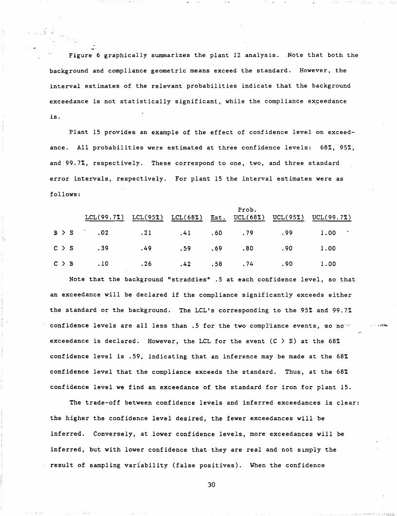
Figure 6 graphically summarizes the plant 12 analysis. Note that both the

background and compliance geometric means exceed the standard. However, the

interval estimates of the relevant probabilities indicate that the background

exceedance is not statistically significant, while the compliance ex~eedance

is.

Plant 15 provides an example of the effect of confidence level on exceed-

ance. All probabilities were estimated at three confidence levels: 68%, 95%,

and 99.7%, respectively. These correspond to one, two, and three standard

error intervals, respectively. For plant 15 the interval estimates were as

follows:

ProbeLCL(99.7%) LCL(95%) LCL(68%) Est. UCL(68%) UCL(95%) UCL(99.7%)

B > S .02 .21 .41 .60 .79 .99 1.00

C > S .39 .49 .59 .69 .80 .90 1.00

C > B .10 .26 .42 .58 .74 .90 1.00

Note that the .background "straddles" .5 at each confidence level, so that

an exceedance will be declared if the compliance significantly exceeds either

the standard or the background. The LCL's corresponding to the 95% and 99.7%

confidence levels are all less than .5 for the two compl'iance events ,'SO 'ncf<~' ","-

exceedance is declared. However, the LCL for the event (C > S) at the 68%

confidence level is .59, indicating that an inference may be made at the 68%

confidence level that the compliance exceeds the standard. Thus, at the 68%

confidence level we find an exceedance of the standard for iron for plant 15.

The trade-off between confidence levels and inferred exceedances is clear:

the higher the confidence level desired, the fewer exceedances will be

inferred. Conversely, at lower confidence levels, more exceedances will be

inferred, but with lower confidence that they are real and not s1mply the

result of sampling variability (false positives). When the confidence

30

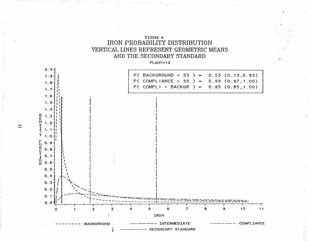
FIGURE 6IRON PROBABILITY DISTRIBUTION

VERTICAL LINES REPRESENT GEOMETRIC MEANSAND TIlE SECONDARY STANDARD

PLANT-12~, : ,

1 1

0.53 (0.13,0.93)0.99 (0.97,1.00)0.95 (0.85,1.00)

PC BACKGROUND> 5S ) ­PC COMPLIANCE> SS ) ­PC COMPLI > BACKGR ) ~

0.5-

2.0-

1. 9- ,La

,II'

1.7 I'I',1. 6- I,1. 5- ,

I1. 4- I

I1. 3- I

I1. 2- ,,1. 1 -

,1.0-

0.9-

oENsITY

FU

~ O. a - ~T ,I 0.7- ,

o O. 6 - ,N ,\\\

0.4- ,r--,'

0.3- I ,\"~:~ I "~_\~'::-:~~~~_=~~ _

[/ l- __ _ .

o 0 ~ I - - ... - - - - - - - - - - - - -1- - - - - - - - - - - =-=-_-::-::. =-=---=-=' =-=--~=-:-.. I I I; 'I I 'I

o 1 2 :f 4 5 & 7 a 9 10

w.....

i' IRON

- - - - - - - -. BACKG ROUND '.

ji- - - - INTERMEDIATE

SECONDARY STANDARD

-----. COMPLIANCE

-intervals are as wide as those for Plant 15 and the conclusion regarding

exceedance is sensitive to the confidence level, the need for additional

information is apparent.

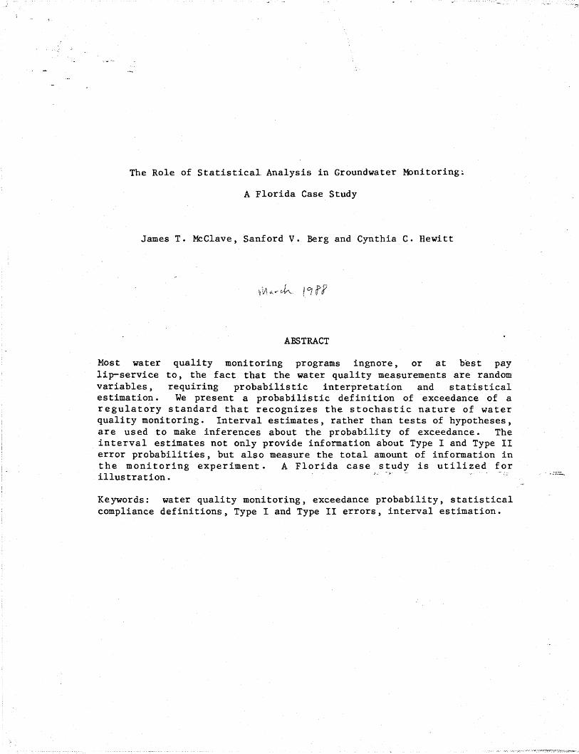
5.2 Evaluation of Parameter Exceedances

Similar analyses were conducted for the other eleven secondary standard

parameters. The chart in Figure 7 shows the number of exceedances for each

parameter at the 95% confidence level. Note that the data reveal no

exceedances for copper, zinc, or foaming agents at any of the confidence

levels. At the 95% confidence level, approximately 10-20% of the facilities

are in exceedance for: chloride, corrosivity, iron, manganese, odor, pH, and

sulfate. About 40% of the plants are in exceedance for color and total

dissolved solids at the 95% confidence level. A comparison of the geometric

means and the declared exceedances reveals that the statistical definition of

exceedance appears to be reasonable. Note that the use of a "one-time

exceedance" or "strict liability" definition would have no associated

statistical confidence level, and the declaredexceedances would bear little

relationship to the geometric means. In contrast, exceedances declared using

the 95% confidence level require significant differences between the compliance-­

geometric mean and the standard (or the compliance and background geometric

means) before an exceedance is declared.

Also shown on Figure 7 is the percentage of facilities that would be

declared in exceedance applying a strict liability definition. A total of 231

exceedances are declared, with virtually every plant in noncompliance for at

least half of the parameters. Strict liability bears little relationship to

the probability distributions from which these parameters are observed, and

therefore has little scientific or statistical validity.

32

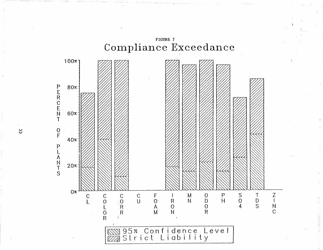
FIGURE 7

COlnpliance Exceedance

P 80~

ERCEN 60~-

T

w awF

40~

pLAN

20~TS

o~I M T ZC C C C F a p s

L a a u a R N D H a D IL R A a a 4 s Na ,R M N R CR

~95% Confidence Level~Strict Liabi I ity

These data can also be used to evaluate how background groundwater

measurements compare to the secondary standards for each parameter. The

background data provide information about the quality of groundwater,

presumably before the plant has any impact. Thus, the comparison of statewide

background to standard provides information about the groundwater quality, as

well as the reasonableness of the standard. Figure 8 shows the percentage of

plants for which the background was found in exceedance of the fixed standard

for each parameter. The parameters which significantly exceed the standard in

background concentrations are color, corrosivity, iron, and pH, with

approximately 50% of the facilities in exceedance for corrosivity and iron, and

about 40% for color and pH. Both odor and total dissolved solids have

geometric means close to-the standard, and are declared in exceedance in about

20% of the plants. The implication is that many of the secondary standard

parameters are present in the groundwater at levels above the standard. Many

of the plants are coastal, which may explain the frequency of background

exceedances for corrosivity and pH.

Causal inferences based on statistical analyses are possible only when the

experiment can be performed in a controlled environment, with the factors

affecting the response under the control of, and varied by, the experimenter.

Since this is rarely the case in monitoring experiments, causal inferences

based on statistical results alone are unjustified. Thus, the conclusion that

the declared exceedances in this analysis are caused by the influence of the

plant cannot be based on the statistical significance of the results.

Inappropriate well locations, natural pockets of high concentration, and

differences between background and compliance flows are just a few potential

causal influences other than the plant that might ~e responsible for

exceedances. Indeed, the intermediate wells often had significantly lower

34

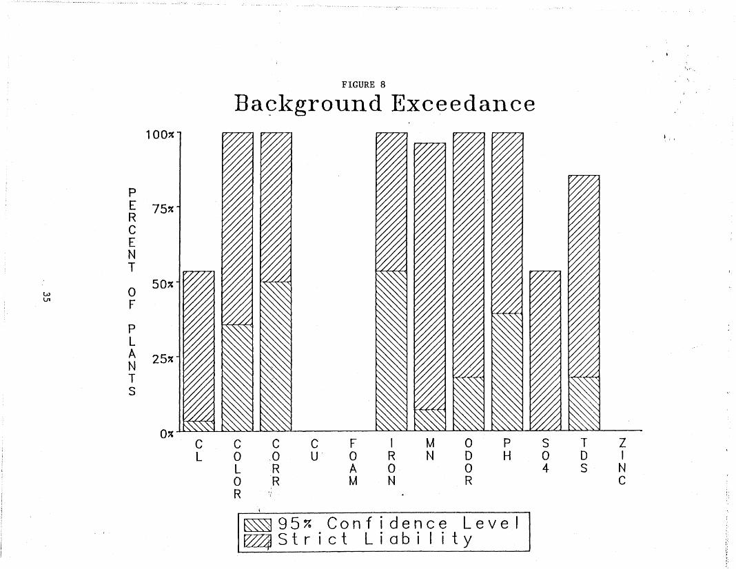
FIGURE 8

Ba9kground Exceedance1OO~

PE 75"RCENT

0 50"wV1

F

pLA 25"NTS

0"I M 0 P T ZC C C C F S

L 0 0 U 0 R N D H 0 0 IL R A 0 0 4 S N0 R M N R CR

1

~95% Confidence Level~Strict Liabi Ii ty

I; ,

· .concentrations than the compliance wells when exceedances were found in the

Floridadata. 1o Since the intermediate wells are located closer to the source,

they would be expected to have levels at least as high as the compliance wells

if the plant were the cause of the exceedance.

The status of secondary standards in Florida remains in question. In

December 1987 the Florida Environmental Regulatory Commission adopted the

standards for new facilities while grandfathering existing facilities, unless

the Department of Environmental Regulation analyses of monitoring data reveals

a significant problem, in which case standards can be imposed on existing

facilities as well. In their presentation to the ERe, DER acknowledged the

need for more rigorous statistical methodology, but correctly pointed out that

these methods need to be developed for primary standards as well. They

furthermore concurred with the FCG report (1987) on the high cost of treatment

for groundwater to c.omply with secondary drinking water standards. The

benefits associated with such investment are extremely difficult to identify,

much less to quantify.

6.0 Conclusion

The definition of noncompliance in groundwater monitoring affects the

scientific validity of groundwater regulations. Probabilistic definitions

offer an objective criteria by which to assess a facility's compliance. In

addition, the probabilistic definition forces regulators to address two

important issues: (1) groundwater parameters are random variables and (2)

policymakers need to specify the percentile of the parameter's distribution

lOTDS is a good example of this phenomena. Plants 3, 4, 12, and 28 wereall declared in exceedance at the 95% confidence level, but in each case thegeometric mean of the intermediate wells was less than that of the compliancewells.

36

-"that constitutes noncompliance, as well as maximum tolerable Type I and Type II

error probabilities. The latter specification enables a sensible

differentiation between health-related and aesthetic standards, where none now

exists, except perhaps in the subjective application of the standards. That

is, a Type I error -- finding an exceedance where none exists -- can result in

mandatory outlays for control technologies, with zero benefit. For aesthetic

standards, analysts would emphasize avoidance of Type I errors. On the other

hand, missing an exceedance of a health-related standard can result in

substantial damages. To limit such damages, avoidance of Type II errors would

be emphasized for health-related parameters.

Although federal and state regulatory agencies are paying increased

attention to the statistical issues of groundwater monitoring, most still focus

(at best) on testing hypotheses about the means of parameter distributions.

The statistical analysis of groundwater monitoring data should focus on the

estimation of exceedance probabilities that define noncompliance. The

lognormal distribution often proves useful for modeling the probability

distribution. The statistical model presented here can be utilized to generate

confidence intervals for the relevant exceedance probabilities. These

intervals better reflect the information in the experiment than tests of

hypotheses. Calculation of intervals for several confidence levels provides

data relevant to the comparison of Type I and Type II error probabilities, and

their effect on the decision regarding noncompliance.

The scientific community appears to be paying increased attention to

statistical issues in environmental monitoring in general and groundwater

monitoring in particular. The recent EPA proposed rule (Federal Register,

August 1987) is certainly a step in the right direction, but still fails to

address directly the issues of noncompliance definition and interval estimation

37

.-as an alternative to hypothesis testing. Also, the EPA proposal skirts the

design issue of the sampling experiment, as has this article. So often the

statistician is confronted with "after the fact" data, the sampling experiment

having been designed and performed by others, usually engineers. Millard

(1987) asserts, "Qualified statisticians simply are not consulted in the

design, analysis, or policy-making phase of environmental-monitoring programs,

or else they are ignored." We would modify this to "almost never" in the

design and policy-making phases, and seldom in the analysis phase. We believe

that the Florida case study provides an example of how involvement in the

analysis phase can be utilized to affect the policy-making phase, and to lay

the groundwork for future involvement in the design phase.

"38

BIBLIOGRAPHY

Berthouex, P. M., (1974). "Some Historical Statistics Related to Future

Standards," J. Environ. Eng. Div., Am. Soc. Civ. Eng., 100.

del Pino, M. P. (1986). "Chemicals and Allied Products," Journal of Water

Pollution Control Federation, 58, 589-594.

Electric Power Research Institute, "Robustness of the ANOVA Model in

Environmental Monitoring Applications," April 1985.

Federal Register, Vol. 51, p. 29812, August 20, 1986.

Federal Register, Vol. 52, p. 31948, August 24, 1987.

Herricks, E. E., Schaeffer, D. J., and Kapsner, J. C. (1985). "Complying with

NPDES permit limits: When is a violation a violation?" Journal of Water

Pollution Control Fed., 57, 109-115.

Landwehr, J. M. (1978). "Some Properties of the Geometric Mean and Its Use in

Water Quality Standards," Water Resources Research, .!i, 467-473.

Loftis, J. C., and Ward, R. C. (1980). "Sampling Frequency Selection for

Regulatory Water Quality Monitoring," Water Resources Bulletin, ~, 501­

507.

Loftis, J. C., Ward, R. C., and Smillie, G. M. (1983). "Statistical models for­

water quality regulation," Journal of Water Pollution Control Federation,

55, 1098-1104.

Mar, B. W., Horner, R. R., Richey, J. S., Palmer, R. N., and Littenmaier, D. P.

(1986). "Data Acquisition Cost-effectiv~ Methods for Obtaining Data on

Water Quality," Environ~ Sci. Technol., 20, 545-551.

Millard, S. P. (1987). "Environmental monitoring, statistics, and the law:

room for improvement," The American Statistician, 41, 249-253.

39

Ward, R. C., and Loftis, J. D. (1983). "Incorporating the Stochastic Nature of

Water Quality into Management," Journal of Water Pollution Control

Federation, ~, 408-414.

Ward,R. C., Loftis, J. C., and McBride, G. B. (1986). "The Data-rich but

Information-poor Syndrome in Water Quality Monitoring," Environmental

Management, lQ, 291-297.

40

APPENDIX A

DERIVATION OF EXCEEDANCE PROBABILITY ESTIMATESAND STANDARD ERRORS

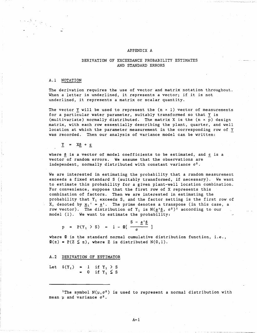
A.1 NOTATION

The derivation requires the use of vector and matrix notation throughout.When a letter is underlined, it represents a vector; if it is notunderlined, it represents a matrix or scalar quantity.

The vector! will be used to represent the (n x 1) vector of measurementsfor a particular water parameter, suitably transformed so that Y is(multivariate) normally distributed. The matrix X is the (n x p) designmatrix, with each row essentially describing the plant, quarter, and welllocation at which the parameter measurement in the corresponding row of Ywas recorded. Then our analysis of variance model can be written:

Y X~ + £:

where ~ is a vector of model coefficients to be estimated, and ~ is avector of random errors. We assume that the observations areindependent, normally distributed with constant variance 0 2 .

We are interested in estimating the probability that a random measurementexceeds a fixed standard S (suitably transformed, if necessary). We wantto estimate this probability for a given plant-well location combination.For convenience, suppose that the first row of X represents thiscombination of factors. Then we are interested in estimating theprobability that Yl exceedsS, and the factor setting is the first row ofX, denoted by Xl' = a'. The prime denotes a transpose (in this case, arow vector). The di;tribution of Yl is N(!'~,02)1 according to 'ourmodel (1). We want to estimate the probability:

S - !'~

p P(Y I > S) 1 - m[o

where m is the standard normal cumulative distribution function, i.e.,m(z) = P(Z ~ z), where Z is distributed N(O,l).

A.2 DERIVATION OF ESTIMATOR

1 if Y1 > So if Y l ~ S

IThe symbol N(~,02) is used to represent a normal distribution withmean ~ and variance 0 2 •

A-I

Then 6(Y 1 ) is an unbiased estimator of the probability of exceedance p,since

P(Y 1 > S) = p

Then according to a corollary to the Rao-Blackwell Theorem (Hogg andCraig, 1978), the minimum variance unbiased estimator (MVUE) for p is theconditional expectation of 6(Y 1 ) given the sufficient statistic for ~.

The sufficient statistic for ~ is the least squares estimator:

The joint probability distribution of Y1 and B is:

where the variance-covariance matrix his:

[(X'X)-l~], .J

(X'X)-l

The conditional distribution of Y1 given ~

normal, withb is (Morrison, 1967)

and

Var[Y 1 I B

~'~ + ~'(X'X)-l(X'X)[~ - ~]a'b

0 2 [1 - a'(X'X)-l(X'X)(X'X)-l a ]0 2 [1 - ~'(X'X)-l~] -

We are now equipped to find the MVUE for p, i.e., the conditionalexpectation of 6(Y 1 ):

B

r 6(y)_CD

1 exp [_[(2n)(1 - ~'(XIX)-1~)].5 0

A-2

Transform using:

y - ~'E

z

Then

r_CD

S - alb <I>(z)dz

S - alb1 - ~[

where we have used <I> to represent the standard normal probability densityfunction,- i. e. ,

<I>(z)1 Z2

-- exp(--2-)I (2n)

Thus, the m~n~mum variance unbiased estimator of p is a standard normalcumulative probability evaluated at the standard S, using an estimatedmean of ~'E, which is just the mean estimated by the model, and anadjusted standard deviation of 0/[1-~'(X'X) I~]. We will denote thisestimator by p.

A.3 DERIVATION OF STANDARD ERROR

We use the Cramer-Rao inequality (Hogg and Craig, 1978) to find an"approximate standard error of the MVUE p. The inequality implies that:

"Var(p)

) aoo

1

where f is the probability density function for Y. Using matrixdifferentiation, we find:

S - ~'~

Const. --2

.50 (! - X~)'(! - X~)

aln{f(!,~)} ,

a~

-2o [X'! - (X'X)~]

A-3

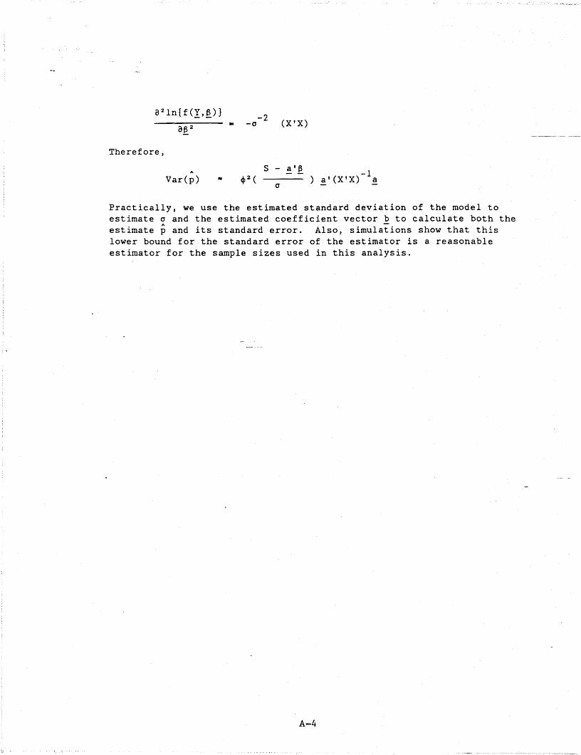
a2ln{f(!,~)J-2

a~2-0 (X'X)

Therefore,

AS - !'~ -1

Var(p) .. ep2( ) !'(X'X) !0

Practically, we use the estimated standard deviation of the model toestimate 0 and the estimated coefficient vector b to calculate both theestimate p and its standard error. Also, simulations show that thislower bound for the standard error of the estimator is a reasonableestimator for the sample sizes used in this analysis.

A-4

Appendix A

BIBLIOGRAPHY

Hogg, R. V., and Craig, A. T. (1978). Introduction to MathematicalStatistics, 4th Edition, Macmillan.

Morrison, D. F. (1967). Multivariate Statistical Methods, McGraw Hill.(p. 88).

A-5