The role of perceptions in pedestrian quality of service

Universidad de los Andes

The role of perceptions in pedestrian quality of service Dissertation

Jose Agustin Vallejo Borda 2-10-2019

i

Evaluator: Prof. Fernando Ramirez, PhD

Evaluator: Prof. Victor Cantillo, PhD

Evaluator: Prof. J. de D. Ortúzar, PhD

Evaluator: Prof. Daniel A. Rodriguez, PhD

Advisor: Prof. Alvaro Rodriguez-Valencia, PhD

Defense date: October 2nd, 2019

Advisor Signature:

ii

Acknowledgements

I would like to thank my family for their constant support during the development of this

doctorate. Special thanks to my fiancée who supported me through difficult times and who

shares the good times with me. I would also like to thank my parents for their constant help

and patience assisting me on the road that I decided to take.

I also thank the team of Grupo de Estudios en Sostenibilidad Urbana y Regional (SUR)

from Universidad de los Andes for their accompaniment in this process. Especially Daniel

Rosas, Hernan Ortiz, and German Barrero, who have been a great support in the

development of this doctorate.

Special thanks to my advisor Alvaro Rodriguez for always being ready to listen and help at

any time. Thank you to Alvaro for being the voice of reason during bad times and for the

constant support offered. I would also like to thank my evaluators, who have accompanied

me throughout this process. I am grateful to professor Fernando Ramirez, who has guided

my academic process with his advice and counsel since the beginning of my

undergraduate studies. To professor Victor Cantillo, who has kindly mentored the

development of this process since its inception. To professor Juan de Dios Ortúzar, who

has always supported me and who generously accepted me into his university to assist my

doctoral process. To professor Daniel Rodriguez, who advised me at the beginning of my

doctoral research and who was essential in the construction of a strong base on which this

study has developed.

I would also like to thank professors Juan Antonio Carrasco and Ricardo Hurtubia, whose

advice led to the development of a successful research. Similarly, thanks to professors

Hernando Vargas, Mauricio Sanchez, Felipe Muñoz, and Juan Enrique Coeymans, who

guided and supported me effectively in the most difficult stages of my doctoral process.

I also would like to thank Colciencias, the Vice-presidency of Research and Creation and

the Faculty of Engineering at Universidad de los Andes, for financing my doctoral

research.

iii

Executive summary

There are many types of pedestrian performance or service indicators (PPSI) that have

been applied worldwide to evaluate the service provided to pedestrians by urban

sidewalks, such as the pedestrian level of service (PLOS) or the quality of service (QoS).

Different inputs have also been used to explain the PPSI considering three groups of

attributes: objective attributes, expert judgement, and the flow-capacity relation. In this

thesis, it was identified variety of predictors (environmental, sociodemographic, physical,

and perceptual) that can potentially be used to explain PPSI.

However, the literature suggests that the methodologies tend to be site dependent (Hasan,

Siddique, Hadiuzzaman, & Musabbir, 2015) and there are not many studies that compare

their forecasting potential. Similarly, when considering predictors (environmental,

sociodemographic, physical, and perceptual), there are not many studies that quantify the

pure and joint effects of each group on the variance explanation of the perceived QoS. In

addition, to explain the way that pedestrians perceive the PPSI considering the

interactions they have when walking, a structural equation model (SEM) was developed by

Geetha Rajendran Bivina & Parida (2019), where some latent variables positive effects on

the PLOS are explained.

For this reason, the aims of this thesis were: firstly, to test the forecasting performance of

some methodologies identified to calculate the PPSI considering the categories of different

inputs (flow-capacity relation, objective data, and perceptual information). Secondly, to

analyze their applicability to Bogotá’s local context. Thirdly, to analyze the individual and

joint effect of the different groups of predictors (environmental, sociodemographic,

physical, and perceptual) on the perceived QoS. Fourthly, to develop a cognitive map that

describes how pedestrians perceive their QoS considering the positive and negative

effects over them when walking. Fifthly, to propose a model to forecast sidewalk QoS

(SQoS) using objective (e.g., physical) and subjective (e.g., perceptions) attributes.

To fulfill the objectives of this research, 1056 pedestrian responses were gathered,

considering their perceptions when walking, including their perception of the SQoS. In

addition, data related to objective on-site attributes, was collected for 30 different

sidewalks in the city of Bogotá. Then, to calculate the methodologies’ performance in

iv

Bogotá, the PPSI values were calculated using 28 different methodologies and compared

with the pedestrian perception of the SQoS. Performance was evaluated through a match

score calculation (the number of matches between the predicted value and the pedestrian

perception of their QoS), by the difference between the predicted value and the

pedestrian’s QoS perception, and by a 𝜒2 test (which compares the forecasted value

distribution and the SQoS data distribution). To analyze pure and joint effects of the

different groups of predictors on the perceived QoS, 15 different models were developed

that considered the groups individually, in pairs, and as groups of three and four. Then, for

each of these models, the partial coefficient of determination (R2) was used to identify the

boundaries of the variance explanation for each group of attributes. Similarly, to quantify

the proportion of the variance that is explained for each model adjusting for the number of

explanatory terms and to test if all coefficients were significant, an adjusted R2 and an F-

test were used respectively. In addition, a SEM approach, using the data on pedestrian’s

perceptions, was used to propose a cognitive map that explains the way in which the QoS

is perceived by pedestrians. Finally, in order to find the best model to forecast the SQoS,

the dataset was divided into two parts: 70% to estimate the various forecasting models

and 30% to validate them. The forecasting models were estimated using four different

approaches: ordinary least squares (OLS), ordered probit, continuous multiple indicators

and multiple causes (MIMIC), and ordered probit MIMIC. Then, the different models were

validated and compared in terms of three measures mentioned above.

The methodologies that better represent Bogotá’s local conditions in terms of match score

were those based on expert judgment (mean = 32.78%). Of these methodologies, one

proposed by Jaskiewicz (1999) was able to predict the SQoS of 15 out of 30 sidewalks in

Bogotá. The second-most effective methodologies, based on match score, were those that

use on-site objective attributes (mean = 22.14%). Of these, one proposed by Talavera-

Garcia & Soria-Lara (2015) was able to predict the SQoS of 14 out of 30 sidewalks.

Finally, the methodologies based on the flow-capacity relationship, had the lowest

capability to evaluate Bogotá’s local conditions (mean = 8.75%). Of these methodologies,

one proposed by the Alcaldia Mayor de Bogota D.C. (2005) was able to predict the SQoS

of eight out of 30 of the city’s sidewalks. This is a version of the method proposed by the

Transportation Research Board (2000) calibrated for the city of Bogotá; interestingly, when

directly applied to Bogotá, it was able to predict only one out of 30 sidewalks (implying an

increase of 23.33 percentual points when the methodology is calibrated to the city).

v

When the individual and joint effects of the different groups of predictors were considered,

it was found that the perception attributes explained the majority of the total variance of the

perceived QoS (between 0.372 and 0.579). The physical attributes explained between

0.021 and 0.225 of the total variance of the perceived QoS, the sociodemographic

attributes explained only between 0.007 and 0.024, and the environmental attributes even

less (between 0.003 and 0.010). Using the cognitive map to understand how pedestrians

perceived the QoS, four latent variables were found that positively influenced pedestrians’

perceptions (sidewalk characteristics, surroundings, protection, and amenities). On the

other hand, three latent variables were found that negatively influenced the QoS

perception by pedestrians (externalities, discomfort, and bike hassles). Finding these

latent variables shows how cognitive maps can be used to understand how pedestrians

perceived the QoS.

An analysis of the forecasting models revealed that the best performance indicators were

obtained when using an ordered probit model to forecast the SQoS (match score =

96.67%, IQR = 0.705, 𝜒2 = 1.167). The OLS model received the second-best performance

indicators (match score = 96.67%, IQR = 0.740, 𝜒2 = 1.543). However, to apply these

models we require both objective (sidewalk and user attributes) and subjective (pedestrian

perceptions) information. Of the models that only need user and sidewalk objective

attributes to both explain the subjective attributes and forecast the SQoS, the ordered

probit MIMIC was the best option (match score = 86.67%, IQR = 0.990, 𝜒2 = 1.281) and

the continuous MIMIC received the worst results (match score = 83.33%, IQR = 1.343, 𝜒2

= 3.848).

We found that a direct application of methodologies to calculate the PPSI proposed in the

literature would not provide a good representation of Bogotá’s local context.

Notwithstanding, we found that those based on expert judgment (subjective attributes)

provided the better results (for calculating the PPSI) when they were directly applied in the

city. In addition, we also found that calibrating the methodologies for the local context

improves their performance. For this reason, to improve the performance of the forecasting

of pedestrian perceived QoS, it is essential to understand the role and impact of subjective

attributes on the perceived QoS and to create methodologies that consider the local

context. Furthermore, the explanatory power of different groups of predictors were

quantified and it was found that perceptual attributes have the highest boundaries of QoS

proportion of the variance explained. However, to forecast the QoS or SQoS, it is

vi

recommended that all groups of attributes are used, considering that all contribute to the

QoS variance explanation. Moreover, a cognitive map is presented that can potentially be

used to describe the effects of the perception of on-site objective attributes on the latent

variables found here, and in the pedestrian perception of the QoS. Finally, using the

ordered probit MIMIC to forecast the SQoS with both objective and subjective attributes, it

is possible to design pedestrian infrastructure that improves the walking experience and

counteracts the negative effects experienced by pedestrians when walking. Additionally,

this model can be used for practitioners, who can apply it to forecast the SQoS using only

objective attributes from the users and the sidewalk.

On this study there are presented many evidences about the role of perceptions to explain

or forecast the pedestrian QoS when walking. Using these evidences, it is possible to

going deeper to continue with the expansion of knowledge in this area. First, it is

recommended to explore other terms referring to the service that an infrastructure is

rendering to its users like comfort, pleasure, stress, experience, or satisfaction. Second,

the use of an ordered probit MIMIC approach to forecast the perceived QoS for urban

sidewalks can be used as a base to propose other forecasting models considering the

perceptual differences between the people of different cities. In addition, the MIMIC

approach can be also proposed to develop a model to forecast the pedestrian perception

of their QoS rather than the complete urban SQoS. Finally, this study can be used also a

base to understand how different is perceived the SQoS considering the differences

between pedestrians (e.g., sex, marital status, etc.).

vii

Resumen ejecutivo

A nivel mundial se han desarrollado diversos indicadores para evaluar el desempeño o

servicio de infraestructura peatonal (PPSI) en aceras urbanas, tales como el nivel de

servicio peatonal (PLOS) o la calidad de servicio (QoS). Para el desarrollo de estas

metodologías se han utilizado diferentes aproximaciones donde se consideran

principalmente tres tipos de atributos para explicar los PPSI (relación flujo-capacidad,

atributos objetivos y juicio de expertos). De estos grupos se han identificado una variedad

de predictores (ambientales, sociodemográficos, físicos y de percepción) que tienen

potencial de ser utilizados para explicar la percepción de QoS.

Sin embargo, a partir de la literatura se puede sugerir que el desempeño de las diversas

metodologías dependen del sitio en el cual son aplicadas (Hasan et al., 2015).

Adicionalmente, no existen muchos estudios que comparen los resultados de las

predicciones de las metodologías considerando la aproximación de cada una de ellas.

Cuando se consideran los predictores tampoco hay muchos estudios que cuantifiquen el

efecto individual y en conjunto de los diferentes grupos de predictores en términos de la

explicación de la varianza de la QoS percibida. Adicionalmente, cuando se busca explicar

la manera en la cual los peatones perciben los PPSI considerando sus interacciones al

caminar, Geetha Rajendran Bivina & Parida (2019) desarrollaron un modelo de

ecuaciones estructurales (SEM) donde de explican únicamente los efectos positivos sobre

el PLOS generados por las percepciones de los peatones al caminar.

Por esta razón, esta investigación tiene como propósitos primero probar el desempeño de

las diferentes metodologías para calcular los PPSI considerando las diferentes

aproximaciones de estas. A partir de este desempeño también se busca analizar la

aplicación de estas metodologías en la ciudad de Bogotá. De igual manera, se busca

analizar el efecto individual y en conjunto de los diferentes grupos de predictores

(ambientales, sociodemográficos, físicos y de percepción) sobre la QoS percibida.

Posteriormente, se busca desarrollar un mapa cognitivo que describa la forma en la cual

los peatones perciben su QoS a partir de los efectos positivos y negativos resultantes de

las interacciones de los peatones al caminar. Finalmente, se busca proponer un modelo

para pronosticar la QoS de las aceras utilizando atributos objetivos y subjetivos.

viii

Para cumplir los objetivos de esta investigación inicialmente se recolectaron 1056

respuestas de peatones referentes a sus percepciones al caminar incluyendo su

percepción sobre la QoS de la acera al igual que datos objetivos en el sitio en 30 aceras

diferentes de la ciudad de Bogotá. Para calcular el desempeño de las diferentes

metodologías en la ciudad de Bogotá se compararon los valores de PPSI resultantes de la

aplicación de cada metodología con las percepciones peatonales sobre su QoS.

Posteriormente, el desempeño se evaluó a partir a partir del cálculo del puntaje de

emparejamiento (número de veces en la cual el valor de la metodología coincide con la

percepción peatonal sobre su QoS) y la variabilidad del error (diferencia entre el valor de

la metodología y la percepción peatonal sobre su QoS).

Para analizar el efecto individual y en conjunto de los diferentes grupos de predictores

sobre la QoS percibida se desarrollaron quince modelos diferentes considerando los

grupos de manera individual, en parejas, tríos y cuartetos. Posteriormente, se calculó el

coeficiente de determinación (r-cuadrado) parcial de cada uno de los modelos

mencionados anteriormente para encontrar los limites superior e inferior de la varianza

explicada por cada uno de los grupos. De forma similar, se utilizó el r-cuadrado ajustado y

la prueba F para cuantificar la explicación de la varianza de cada modelo ajustando por el

número de variables independientes y para conocer la significancia de los coeficientes de

los modelos respectivamente. A continuación, con el fin de proponer un mapa cognitivo

que pudiera explicar la forma en la cual la QoS es percibida por los peatones se utilizó un

SEM a partir de las percepciones peatonales.

Finalmente, para proponer un modelo que permita pronosticar la QoS en aceras

inicialmente se dividió el conjunto de datos en dos: 70% para desarrollar los modelos de

pronóstico y 30% para validarlos. Los modelos de pronóstico se desarrollaron a partir de

cuatro aproximaciones diferentes: mínimos cuadrados ordinarios (MCO), probit

ordenados, múltiples indicadores y múltiples causas (MIMIC) continuo y MIMIC probit

ordenados. Posteriormente, los diferentes modelos fueron validados y comparados

utilizando el puntaje de emparejamiento, la variabilidad del error y la prueba de 𝜒2

(comparación entre la distribución de los valores pronosticados de la QoS y la distribución

de los datos observados de QoS).

Las metodologías que mejor representan las condiciones de Bogotá considerando el

puntaje de emparejamiento son aquellas basadas en juicio de expertos (media = 32.78%).

ix

De estas metodologías se encontró que la propuesta por Jaskiewicz (1999) puede

pronosticar la QoS percibida en 15 de cada 30 aceras en Bogotá. En segunda posición

considerando el puntaje de emparejamiento se encuentran las metodologías basadas en

atributos objetivos (media = 22.14%). De estas metodologías se encontró que la

propuesta por Talavera-Garcia & Soria-Lara (2015) puedes pronosticar la QoS percibida

en 14 de cada 30 aceras en Bogotá. Finalmente, las metodologías basadas en la relación

flujo-capacidad son las que tienen menor capacidad de evaluar las condiciones locales de

Bogotá en términos de pronóstico de QoS (media = 8.75%). De estas metodologías se

encontró que la propuesta por la Alcaldia Mayor de Bogota D.C. (2005) puede pronosticar

la QoS percibida en 8 de cada 30 aceras en Bogotá. La metodología propuesta por la

Alcaldia Mayor de Bogota D.C. (2005) es una versión calibrada para la ciudad de Bogotá

de la metodología propuesta por el Transportation Research Board (2000) la cual al ser

aplicada directamente puede pronosticar 1 de cada 30 aceras en Bogotá. Esto quiere

decir que la calibración desarrollada permitió un incremento de 23.33 puntos porcentuales

probando los beneficios sobre la capacidad de las metodologías que se pueden generar a

partir de calibraciones considerando el contexto local.

Cuando se consideran los efectos individuales y en conjunto de los diferentes grupos de

predictores, se encontró que los atributos de percepción son los que mayor variabilidad

explican de la QoS percibida (entre 0.372 y 0.579). En segundo lugar, los atributos físicos

son los que siguen en cantidad de explicación de la variabilidad total de la QoS percibida

(entre 0.021 y 0.225). Posteriormente, los atributos sociodemográficos son unos de los

que menos explican la variabilidad total de la QoS percibida (entre 0.007 y 0.024).

Finalmente, los atributos ambientales son los que menos explican la variabilidad total de

la QoS percibida (entre 0.003 y 0.010). Considerando el desarrollo del mapa cognitivo

para entender como los peatones perciben su QoS se encontraron cuatro variables

latentes que influencian positivamente la QoS que perciben los peatones (características

de la acera, alrededores, protección y servicios e instalaciones). Por otro lado, se

encontraron tres variables latentes que influencian negativamente la QoS percibida por los

peatones (externalidades, incomodidad y molestias con bicicletas). A partir de las

variables latentes descubiertas se propone el mapa cognitivo que se puede utilizar para

entender como los peatones perciben su QoS.

Considerando los modelos de pronóstico, cuando se busca pronosticar la QoS de la acera

a partir del modelo probit ordenado se obtienen los mejores indicadores de desempeño al

x

ser validado (puntaje de emparejamiento = 96.67%, RQ = 0.705, 𝜒2=1.167). En términos

de indicadores de desempeño, el modelo MCO se localiza en segunda posición (puntaje

de emparejamiento = 96.67%, RQ = 0.740, 𝜒2=1.543). Sin embargo, para aplicar estos

modelos se necesita obtener información tanto objetiva como subjetiva. Al considerar

modelos que solo necesiten como variables de entrada datos objetivos de los usuarios y

las aceras para pronosticar la QoS, el modelo MIMIC probit ordenado se localiza en

primera posición (puntaje de emparejamiento = 86.67%, RQ = 0.990, 𝜒2=1.281).

Finalmente, el modelo MIMIC continuo se localiza en última posición (puntaje de

emparejamiento = 83.33%, RQ = 1.343, 𝜒2=3.848).

A partir de esta investigación se encontró que al aplicar en Bogotá directamente las

diversas metodologías propuestas en la literatura para calcular los PPSI no se obtiene

una buena representación del contexto local de la ciudad. Sin embargo, se encontró que

de las metodologías existentes aquellas que se basan en juicio de expertos (atributos

subjetivos) son las que proveen mejores resultados al calcular el PPSI directamente en

Bogotá. Adicionalmente, se encontró que el calibrar las metodologías al contexto local

mejora el desempeño de las metodologías. Por estas razones, se encontró que el

entender el rol e impacto de los atributos subjetivos sobre la calidad de servicio percibida

y generar metodologías considerando el contexto local mejorará el desempeño del cálculo

de la QoS percibida por los peatones. Adicionalmente, se cuantificó el poder explicativo

de diferentes grupos de predictores donde los atributos de percepción son aquellos que

tienen los limites inferiores y superiores de mayor magnitud al explicar la variabilidad de la

QoS percibida. A pesar de esto, para pronosticar la QoS percibida en las aceras se

recomienda la utilización de todos los grupos de atributos debido a que todos ellos

aportan a la explicación de la variabilidad de la QoS percibida. Adicionalmente, se

presenta un mapa cognitivo con potencial de ser utilizado para describir los efectos de las

percepciones peatonales sobre atributos objetivos y la QoS a partir de las variables

latentes encontradas. Finalmente, es posible desarrollar infraestructura peatonal que

mejore la experiencia de caminata de los peatones y que mitigue los efectos negativos

que se pueden generar sobre los peatones al caminar, a partir del modelo propuesto para

pronosticar la QoS en aceras. Adicionalmente, se propone un modelo para la utilización

por parte de profesionales que puede ser aplicado para predecir la QoS de las aceras a

partir de variables objetivas de los usuarios y aceras donde ya se han involucrado las

percepciones de los peatones (MIMIC probit ordenado).

xi

En este estudio se presentan evidencias sobre el rol que tienen las percepciones para

explicar y pronosticar la QoS de los peatones al caminar. Por medio de estas evidencias,

es posible profundizar en la investigación para continuar con la expansión del

conocimiento en esta área. Primero, se recomienda explorar otros términos que se

refieren al servicio que una infraestructura peatonal le provee a sus usuarios como lo son

el confort, placer, estrés, experiencia o satisfacción. Segundo, el uso de un modelo MIMIC

probit ordenado para pronosticar como los peatones perciben la QoS de una acera urbana

se puede utilizar como base para proponer otros modelos de pronóstico considerando las

diferencias de percepción existentes entre las personas de diferentes ciudades.

Adicionalmente, los modelos MIMIC también pueden ser utilizados como base para

proponer modelos de pronóstico enfocados en el individuo mas que en la acera completa.

Finalmente, este estudio puede ser utilizado como base para entender las diferencias que

pueden existir sobre la percepción de la QoS de la acera basados en las diferencias que

se pueden presentar entre los peatones (e.g., sexo, estado civil, etc.).

xii

Publications

Through the development of this doctoral research we prepared publications for journals

and conferences. There are nine journal publications proposed of which five are under

review and four are papers in process to be submitted. We also attended five conferences

already and there is one other conference in process to be attended.

Journal papers

• Vallejo-Borda, J.A., Rosas-Satizabal, D. & Rodriguez-Valencia, A. (2019). Do

attitudes and perceptions help to explain bicycle infrastructure quality of service?

Transportation Research Part D: Transport and Environment (under review)

• Vallejo-Borda, J. A., Ortiz-Ramirez, H.A., Rodriguez-Valencia, A., Hurtubia, R. &

Ortúzar, J. de D. (2019). Forecasting the quality of service of Bogota’s sidewalks:

an ordered probit MIMIC approach. Transportation Research Record (in-Press)

• Rodriguez-Valencia, A., Barrero, G.A., Ortiz-Ramirez, H.A. & Vallejo-Borda, J.A.

(2019). The power of users’ perceptions in pedestrian quality of service.

Transportation Research Record (under review).

• Vallejo-Borda, J.A., Cantillo, V. & Rodriguez-Valencia, A. (2019). A perception

based cognitive map of the pedestrian perceived quality of service on urban

sidewalks. Transportation Research Part F: Traffic Psychology and Behaviour

(under review).

• Vallejo-Borda, J.A., Ortiz-Ramirez, H.A., Rodriguez-Valencia, A., Cantillo, V. &

Ortuzar, J. de D. (2019). Perception based methodological approaches to forecast

the pedestrian quality of service on urban sidewalks. Transportation Research Part

B: Methodological (working paper).

xiii

• Ortiz-Ramirez, H.A., Vallejo-Borda, J.A. & Rodriguez-Valencia, A. (2019). Testing

the Mehrabian-Russell model in pedestrian approach-avoidance behavior when

walking on urban sidewalks. Journal of Environmental Psychology (working paper).


(2019). The power of users’ perceptions: pedestrian and bicycle level of service

and quality of service revisited. International Journal of Sustainable Transportation

(working paper).

• Vallejo-Borda, J.A., Cantillo, V., Rodriguez-Valencia, A., Eboli, L., Forciniti, C. &

Mazzulla, G. (2019). Effects of perceptions in pedestrian quality of service: a

literature review. Transport Reviews (working paper).

Conferences

• Vallejo-Borda, J.A., Ortiz-Ramirez, H.A., Rodriguez-Valencia, A., Hurtubia, R. &

Ortúzar, J. de D. (2019). Forecasting the quality of service of Bogota’s sidewalks:

an ordered probit MIMIC approach. 2020 TRB Annual Meeting. Washington, D.C.,

USA (to be attended).


(2019). The power of users’ perceptions in pedestrian quality of service. 2020 TRB

Annual Meeting. Washington, D.C., USA (to be attended).

• Vallejo-Borda, J.A. & Rodriguez-Valencia, A. (2019). Mapa cognitivo peatonal

sobre la calidad de servicio percibida en aceras urbanas. XIII Congreso

Colombiano de Transporte y Tránsito. Cartagena, Colombia.

• Vallejo-Borda, J.A., Rosas-Satizabal, D. & Rodriguez-Valencia, A. (2019). Calidad

de servicio de infraestructura para bicicletas: una aproximación desde las

percepciones de los ciclistas. XIII Congreso Colombiano de Transporte y Tránsito.

Cartagena, Colombia.

xiv

• Vallejo-Borda, J.A., Rosas-Satizabal, D. & Rodriguez-Valencia, A. (2019).

Cyclists’ perceived infrastructure service quality and enjoyment: a SEM approach.

2019 TRB Annual Meeting. Washington, D.C., USA.

• Vallejo-Borda, J.A. & Rodriguez-Valencia, A. (2018). Siguiendo el rastro de las

percepciones en el cálculo del nivel de servicio peatonal (P-LOS) en andenes

urbanos. XX Congreso Panamericano de Ingeniería de Tránsito, Transporte y

Logística. Medellín, Colombia.

• Rodriguez-Valencia, A., Paris, D. & Vallejo-Borda, J.A. (2017). Uso de

percepciones para determinar el nivel de servicio peatonal: caso carrera séptima,

Bogotá, Colombia. 18° Congreso Chileno de Ingeniería de Transporte. La Serena,

Chile.

• Rodriguez-Valencia, A., Paris, D. & Vallejo-Borda, J.A. (2017). Relación entre

percepción y nivel de servicio peatonal: caso carrera 7ma Bogotá, Colombia. XII

Congreso Colombiano de Transporte y Tránsito. Bogotá, Colombia.

xv

Contents

Abbreviations .................................................................................................................................... xvi

Tables content .................................................................................................................................. xvii

Figures content.................................................................................................................................. xix

1. Introduction ................................................................................................................................ 1

2. Literature review ......................................................................................................................... 4

3. Methodology ............................................................................................................................. 14

3.1 Literature review process .................................................................................................. 14

3.2 Data collection................................................................................................................... 15

3.3 Modelling approach .......................................................................................................... 22

3.3.1. Ordinary least squares (OLS) models ........................................................................ 22

3.3.2. Ordered probit models .............................................................................................. 23

3.3.3. Structural equation modeling (SEM) ......................................................................... 24

3.3.4. Multiple indicator multiple cause (MIMIC) models .................................................. 25

3.3.5. Multi-attribute utility theory (MAUT) ....................................................................... 26

3.4 Performance indicators ..................................................................................................... 26

3.5 Methodological performance evaluation process ............................................................ 27

3.6 Determining how and to what extent perceptions influence the perceived QoS ............ 28

3.7 Forecasting the perceived QoS ......................................................................................... 29

3.8 Study limitations................................................................................................................ 29

4. Performance of the PPSI methodologies in Bogotá’s urban context ........................................ 30

5. The influence of perceptions on the QoS .................................................................................. 43

6. Application of pedestrian perceptions for QoS forecasting ...................................................... 57

7. Discussion and analysis ............................................................................................................. 71

8. Conclusions, recommendations, and further research ............................................................. 79

8.1 Conclusions ....................................................................................................................... 79

8.2 Recommendations and further research .......................................................................... 80

9. References ................................................................................................................................. 82

10. Appendix A – Sidewalk sample .............................................................................................. 88

11. Appendix B – Methodological review ................................................................................. 103

xvi

Abbreviations

A: Average pedestrian age

BP: Bicyclist presence

BW: Buffer width

DP: Driveway length

HGV: Heavy goods vehicles

HP: Potholes presence

LOS: Level of service

MAUT: Multi-Attribute Utility Theory

MIMIC: Multiple Indicators and Multiple Causes

MSP: Median street presence

OLS: Ordinary least squares

PLOS: Pedestrian level of service

PPSI: Pedestrian performance or service indicators

QoS: Quality of service

R2: Coefficient of determination

SEM: Structural equation modelling

SQoS: Sidewalk quality of service

SW: Sidewalk width

xvii

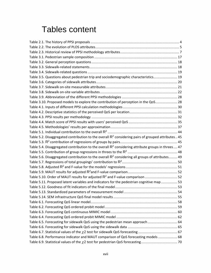
Tables content

Table 2.1. The history of PPSI proposals ............................................................................................. 4

Table 2.2. The evolution of PLOS attributes ........................................................................................ 5

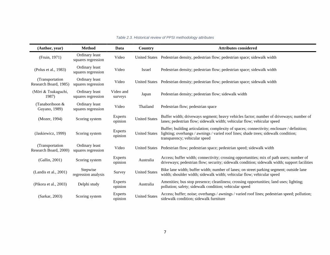
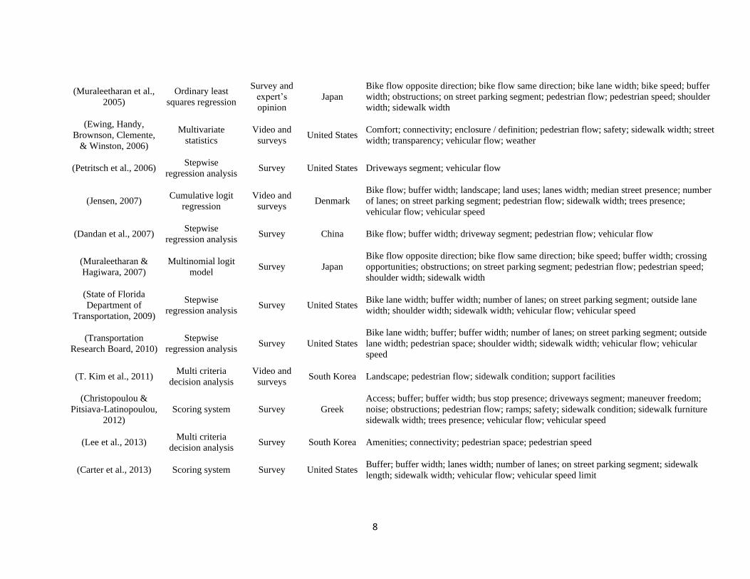
Table 2.3. Historical review of PPSI methodology attributes .............................................................. 7

Table 3.1. Pedestrian sample composition ....................................................................................... 17

Table 3.2. General perception questions .......................................................................................... 18

Table 3.3. Sidewalk-related statements ............................................................................................ 18

Table 3.4. Sidewalk-related questions .............................................................................................. 19

Table 3.5. Questions about pedestrian trip and sociodemographic characteristics......................... 19

Table 3.6. Categories of sidewalk attributes ..................................................................................... 20

Table 3.7. Sidewalk on-site measurable attributes ........................................................................... 21

Table 3.8. Sidewalk on-site variable attributes ................................................................................. 22

Table 3.9. Abbreviation of the different PPSI methodologies .......................................................... 28

Table 3.10. Proposed models to explore the contribution of perception in the QoS....................... 28

Table 4.1. Inputs of different PPSI calculation methodologies ......................................................... 30

Table 4.2. Descriptive statistics of the perceived QoS per location .................................................. 31

Table 4.3. PPSI results per methodology .......................................................................................... 32

Table 4.4. Match score of PPSI results with users’ perceived QoS ................................................... 35

Table 4.5. Methodologies’ results per approximation ...................................................................... 37

Table 5.1. Individual contribution to the overall R2 ......................................................................... 44

Table 5.2. Disaggregated contribution to the overall R2 considering pairs of grouped attributes .. 45

Table 5.3. R2 contribution of regressions of groups by pairs............................................................ 45

Table 5.4. Disaggregated contribution to the overall R2 considering attribute groups in threes .... 47

Table 5.5. Contribution of group regressions in threes to the R2 .................................................... 48

Table 5.6. Disaggregated contribution to the overall R2 considering all groups of attributes ......... 49

Table 5.7. Regressions of total groupings’ contribution to R2 .......................................................... 50

Table 5.8. Adjusted R2 and F-value for the models’ regressions ...................................................... 51

Table 5.9. MAUT results for adjusted R2and F-value comparison .................................................... 52

Table 5.10. Order of MAUT results for adjusted R2 and F-value comparison .................................. 52

Table 5.11. Proposed latent variables and indicators for the pedestrian cognitive map ................. 53

Table 5.12. Goodness of fit indicators of the final model ................................................................. 53

Table 5.13. Standardized parameters of measurement model ........................................................ 54

Table 5.14. SEM infrastructure QoS final model results ................................................................... 55

Table 6.1. Forecasting QoS linear model........................................................................................... 58

Table 6.2. Forecasting QoS ordered probit model ............................................................................ 59

Table 6.3. Forecasting QoS continuous MIMIC model ...................................................................... 60

Table 6.4. Forecasting QoS ordered probit MIMIC model ................................................................ 62

Table 6.5. Forecasting for sidewalk QoS using the pedestrian mean approach ............................... 64

Table 6.6. Forecasting for sidewalk QoS using the sidewalk data .................................................... 65

Table 6.7. Statistical values of the 𝜒2 test for sidewalk QoS forecasting ......................................... 67

Table 6.8. Performance indicator and MAUT comparison of QoS forecasting models .................... 68

Table 6.9. Statistical values of the 𝜒2 test for pedestrian QoS forecasting ...................................... 70

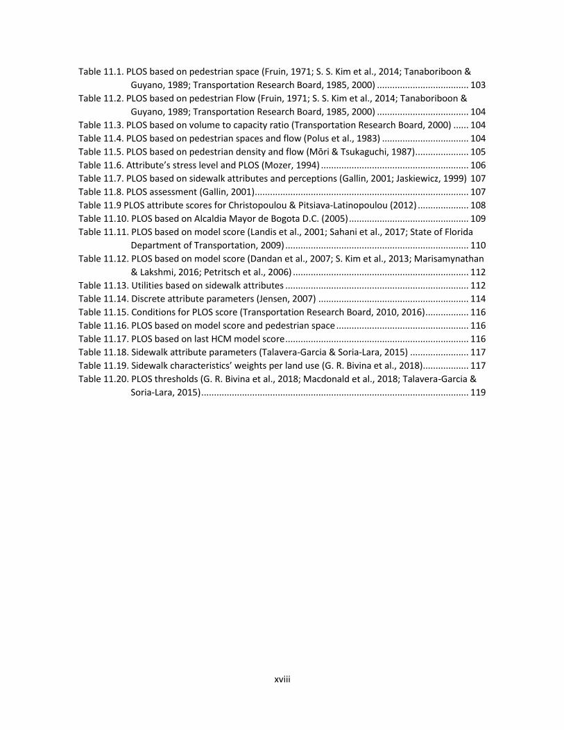
xviii

Table 11.1. PLOS based on pedestrian space (Fruin, 1971; S. S. Kim et al., 2014; Tanaboriboon &

Guyano, 1989; Transportation Research Board, 1985, 2000) .................................... 103

Table 11.2. PLOS based on pedestrian Flow (Fruin, 1971; S. S. Kim et al., 2014; Tanaboriboon &

Guyano, 1989; Transportation Research Board, 1985, 2000) .................................... 104

Table 11.3. PLOS based on volume to capacity ratio (Transportation Research Board, 2000) ...... 104

Table 11.4. PLOS based on pedestrian spaces and flow (Polus et al., 1983) .................................. 104

Table 11.5. PLOS based on pedestrian density and flow (Mōri & Tsukaguchi, 1987) ..................... 105

Table 11.6. Attribute’s stress level and PLOS (Mozer, 1994) .......................................................... 106

Table 11.7. PLOS based on sidewalk attributes and perceptions (Gallin, 2001; Jaskiewicz, 1999) 107

Table 11.8. PLOS assessment (Gallin, 2001) .................................................................................... 107

Table 11.9 PLOS attribute scores for Christopoulou & Pitsiava-Latinopoulou (2012) .................... 108

Table 11.10. PLOS based on Alcaldia Mayor de Bogota D.C. (2005) ............................................... 109

Table 11.11. PLOS based on model score (Landis et al., 2001; Sahani et al., 2017; State of Florida

Department of Transportation, 2009) ........................................................................ 110

Table 11.12. PLOS based on model score (Dandan et al., 2007; S. Kim et al., 2013; Marisamynathan

& Lakshmi, 2016; Petritsch et al., 2006) ..................................................................... 112

Table 11.13. Utilities based on sidewalk attributes ........................................................................ 112

Table 11.14. Discrete attribute parameters (Jensen, 2007) ........................................................... 114

Table 11.15. Conditions for PLOS score (Transportation Research Board, 2010, 2016) ................. 116

Table 11.16. PLOS based on model score and pedestrian space .................................................... 116

Table 11.17. PLOS based on last HCM model score ........................................................................ 116

Table 11.18. Sidewalk attribute parameters (Talavera-Garcia & Soria-Lara, 2015) ....................... 117

Table 11.19. Sidewalk characteristics’ weights per land use (G. R. Bivina et al., 2018).................. 117

Table 11.20. PLOS thresholds (G. R. Bivina et al., 2018; Macdonald et al., 2018; Talavera-Garcia &

Soria-Lara, 2015) ......................................................................................................... 119

xix

Figures content

Figure 2.1. Proposed structure of pedestrians’ perceived QoS ........................................................ 12

Figure 3.1. Literature Review Process ............................................................................................... 15

Figure 3.2. Survey points ................................................................................................................... 16

Figure 3.3. SEM generic model structure .......................................................................................... 24

Figure 3.4. Continuous, ordered, and discrete MIMIC general models ............................................ 25

Figure 4.1. Methodologies’ errors boxplot ....................................................................................... 36

Figure 4.2. Performance of flow-capacity based methodologies ..................................................... 37

Figure 4.3. Flow-capacity relation methodologies errors boxplot .................................................... 38

Figure 4.4. Performance of objective attributes-based methodologies ........................................... 39

Figure 4.5. Objective attributes methodologies errors boxplot ....................................................... 40

Figure 4.6. Performance of expert judgement-based methodologies .............................................. 41

Figure 4.7. Expert judgement-based methodologies errors boxplot ................................................ 41

Figure 5.1. Proportion of the total variance explained by individual group regressions .................. 43

Figure 5.2. Proportion of the total variance explained by group regressions in pairs ...................... 44

Figure 5.3. Proportion of the total variance explained by regressions of the groups of three ........ 46

Figure 5.4. Proportion of the total variance explained by regressions of total groups .................... 49

Figure 5.5. SEM infrastructure QoS final model ................................................................................ 56

Figure 6.1. Performance of proposed forecasting models vs existing methodologies ..................... 57

Figure 6.2. Match of the forecasting models with reported sidewalk QoS confidence interval ...... 66

Figure 6.3. Sidewalks forecasting models’ errors boxplot ................................................................ 67

Figure 6.4. Pedestrians forecasting models’ errors boxplot ............................................................. 69

1

1. Introduction

In recent years, there has been progress toward the better measurement or evaluation of the service, quality or performance of pedestrian infrastructure. Several pedestrian performance or service indicators (PPSI) have been developed, such as the pedestrian level of service (PLOS), which in transportation planning is the most traditional PPSI that seeks to explain how pedestrians are served by the infrastructure. This PPSI is based on the traditional level of service (LOS) which is a qualitative stratification of performance measures that represents the quality of a transport infrastructure. This methodology allows researchers to determine the quality that an infrastructure renders over a certain time on a six-point ordinal scale (Roess & Prassas, 2014; Transportation Research Board, 2000, 2010, 2016). LOS is frequently used for motorized traffic on highways, urban roads, intersections, roundabouts, etc. The main principle behind LOS for motorized vehicles is the demand-capacity relationship (i.e., the level of congestion). Therefore, traffic flow variables like speed, density, and flow are frequently used to calculate the LOS.

The first methodologies for the calculation of PLOS only considered the flow-capacity relationship (Fruin, 1971). In the 2000s, research on PLOS found other factors beyond the demand-capacity analysis that explain pedestrian satisfaction from a walker’s experience of a certain place. The Transportation Research Board (2010) defines eight quantitative criteria that may affect PLOS based on capacity. However, pedestrians usually interact with other transportation modes, sharing more than capacity criteria with the other modes, affecting the perception of PLOS. These interactions are evident in research that identifies the different criteria affecting PLOS. For example, B. Landis, Vattikuti, Ottenberg, McLeod, & Guttenplan, (2001) use vehicle flow variables (flow and speed) and lateral separation to calculate PLOS. Additionally, Pikora, Giles-Corti, Bull, Jamrozik, & Donovan (2003) use criteria like signaling, tree planting, and rest furniture to measure PLOS. Similarly, Jaskiewicz (1999) uses pedestrian interaction with facades and architecture to measure PLOS. Additionally, other authors have shown that criteria like traffic pollution, road safety, and personal security are perceived as variables that affect PLOS (Rodriguez-Valencia, Paris, & Vallejo-Borda, 2017).

Most methods used to calculate the PPSI are usually based on measurable physical features. Furthermore, even the more sophisticated PPSI methods available might still be site-dependent. Hasan, Siddique, Hadiuzzaman, & Musabbir (2015) found that methodologies to calculate PPSI developed in a different place from where they were applied represented at most 72% of the new local conditions; they also found that most of the US-based methodologies represented less than 50% of the local conditions in Dhaka City. However, there are not many studies that identify how current state-of-the-practice methods to evaluate PPSI are able to represent the local conditions of cities in Colombia or other Latin-American countries. Also, it is not possible to be confident in the results of the PPSI methods applied in Bogotá, because these methods do not represent the city’s context and characteristics (Á. Rodríguez & Unda, 2015).

In addition, walking implies a sensorial experience within the surrounding environment that affects the perceived quality of service (QoS), but it is not clear how much of the pedestrian perception of the QoS is explained by their perceptions of the interactions they have when walking. Similarly, it is not clear how pedestrians interact with the sidewalk to later evaluate the QoS from their perceptions.

2

Pedestrian perceptions are not considered much in the literature for the evaluation of the QoS perceived by pedestrians. However, QoS is not what is offered, but what the user receives (Drucker, 2006). Additionally, it can be hypothesized that the perceived QoS is affected by more than objective attributes, and the sensorial experience of pedestrians when walking must be considered. Fernández-Heredia, Jara-Díaz, & Monzón (2016) mentioned that including perceptions in choice models enhanced the model’s goodness of fit and its performance. In addition, an improvement in the understanding of pedestrian perceptions when considering subjective attributes to explain the perceived QoS can create an opportunity for the benefit of pedestrians.

The main objective of this study is to evince the role and effect of pedestrian perceptions on their QoS and on the QoS forecasting on urban sidewalks. For this reason, on this study initially it is going to be tested if PPSI methodologies are in fact site-dependent, by forecasting the PPSI in Bogotá using 28 methodologies proposed worldwide, and comparing them with the pedestrian perceptions of QoS when walking. Then, to explore the power of perceptions that explain the QoS as perceived by pedestrians, different models to explain perceived QoS will be developed by combining different attributes as independent variables in groups (environmental, sociodemographic, physical and perceptual), and calculating goodness-of-fit (i.e. partial R2, adjusted R2, and F statistics). Then, to find out if there are latent variables behind the perceived QoS and the relationships between them, a pedestrian cognitive map will be proposed, explaining the perceived QoS by means of structural equation models (SEM) and using the perceptions recorded. Finally, to develop a sidewalk QoS (SQoS) forecasting model that considers both objective and subjective attributes, four different approaches will be used: OLS (Fruin, 1971; S. Kim, Choi, & Kim, 2013; S. S. Kim, Choi, Kim, & Tay, 2014; Mōri & Tsukaguchi, 1987; Muraleetharan, Adachi, Hagiwara, & Kagaya, 2005; Polus, Schofer, & Ushpiz, 1983; Tanaboriboon & Guyano, 1989; Transportation Research Board, 1985, 2000), ordered probit (Choi, Kim, Min, Lee, & Kim, 2016; Jensen, 2007; Kang & Fricker, 2016; Kang, Xiong, & Mannering, 2013; Muraleetharan & Hagiwara, 2007), and continuous and ordered probit multiple indicator multiple causes (MIMIC) (Geetha Rajendran Bivina & Parida, 2019).

This research also aims to explore the role of users’ perceptions as input variables in the explanation of the quality of service of a sidewalk. The study comprises the following questions: How have users and their perceptions been considered as predictors for service or performance in the past? To what extent can pedestrian perceptions explain the sidewalk QoS? And finally, how can perceptions be applied and what methods are better to forecast QoS? To achieve the main research objective and to answer the questions, the following specific objectives have been established:

• To analyze the role of perceptions and physical attributes in the PPSI calculation.

• To analyze the evolution of the main PPSI methodologies and to evaluate their applicability for Bogotá’s local context.

• To quantify the contribution of perception attributes in the explanation of QoS.

• To propose a perceived QoS cognitive map from pedestrian perceptions.

• To forecast the QoS and SQoS for pedestrians in the city of Bogotá.

This document includes a complete literature review that describes the evolution of PPSI and the interaction between perception and the PPSI. Then, the methodology section explains how the doctoral project was developed. After, the performance results for the 28 PPSI methodologies applied in Bogotá are presented. Subsequently, the contribution of

3

perceptions to the explanation of QoS are quantified and a cognitive map to understand how pedestrians perceive the QoS is proposed. Then, two forecasting models for the SQoS that can be applied on the different sidewalks of Bogotá and one forecasting model to predict the users’ QoS are proposed. Next, the different results of the previous steps are discussed and analyzed. Finally, the conclusions of the study are presented with reference to the research question, the main objective, the specific objectives, the results, and the discussion and analysis sections.

4

2. Literature review Many PPSI have been proposed over the years to evaluate pedestrian performance or

service indicators. PLOS was initially proposed in the 1970s by Fruin (1971) and was

based on the level of service (LOS) methodology developed for motor vehicles by the

Bureau of Public Roads (1950). Then, in the 1980s, PPSI options were expanded by the

addition of quality of service (QoS) as a definition for LOS (Transportation Research

Board, 1985) and pedestrian comfort (Mōri & Tsukaguchi, 1987). In the 1990s, the PPSI

spectrum increased again through the addition of other terms such as stress (Mozer,

1994) and experience (Jaskiewicz, 1999). Finally, in the twenty-first century, the PPSI

spectrum was completed with the addition of the term satisfaction (Jensen, 2007). These

PPSI are usually measured by asking users for their perspective on the overall PPSI

provided by the infrastructure. In addition, the PPSI terms are usually used

interchangeably in the literature to refer to the same output (service) related to pedestrians

(see Table 2.1).

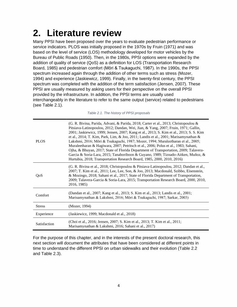
Table 2.1. The history of PPSI proposals

PLOS

(G. R. Bivina, Parida, Advani, & Parida, 2018; Carter et al., 2013; Christopoulou &

Pitsiava-Latinopoulou, 2012; Dandan, Wei, Jian, & Yang, 2007; Fruin, 1971; Gallin,

2001; Jaskiewicz, 1999; Jensen, 2007; Kang et al., 2013; S. Kim et al., 2013; S. S. Kim

et al., 2014; T. Kim, Park, Lim, & Joo, 2011; Landis et al., 2001; Marisamynathan &

Lakshmi, 2016; Mōri & Tsukaguchi, 1987; Mozer, 1994; Muraleetharan et al., 2005;

Muraleetharan & Hagiwara, 2007; Petritsch et al., 2006; Polus et al., 1983; Sahani,

Ojha, & Bhuyan, 2017; State of Florida Department of Transportation, 2009; Talavera-

Garcia & Soria-Lara, 2015; Tanaboriboon & Guyano, 1989; Tiznado-Aitken, Muñoz, &

Hurtubia, 2018; Transportation Research Board, 1985, 2000, 2010, 2016)

QoS

(G. R. Bivina et al., 2018; Christopoulou & Pitsiava-Latinopoulou, 2012; Dandan et al.,

2007; T. Kim et al., 2011; Lee, Lee, Son, & Joo, 2013; Macdonald, Szibbo, Eisenstein,

& Mozingo, 2018; Sahani et al., 2017; State of Florida Department of Transportation,

2009; Talavera-Garcia & Soria-Lara, 2015; Transportation Research Board, 2000, 2010,

2016, 1985)

Comfort (Dandan et al., 2007; Kang et al., 2013; S. Kim et al., 2013; Landis et al., 2001;

Marisamynathan & Lakshmi, 2016; Mōri & Tsukaguchi, 1987; Sarkar, 2003)

Stress (Mozer, 1994)

Experience (Jaskiewicz, 1999; Macdonald et al., 2018)

Satisfaction (Choi et al., 2016; Jensen, 2007; S. Kim et al., 2013; T. Kim et al., 2011;

Marisamynathan & Lakshmi, 2016; Sahani et al., 2017)

For the purpose of this chapter, and in the interests of the present doctoral research, this

next section will document the attributes that have been considered at different points in

time to understand the different PPSI on urban sidewalks and their evolution (Table 2.2

and Table 2.3).

5

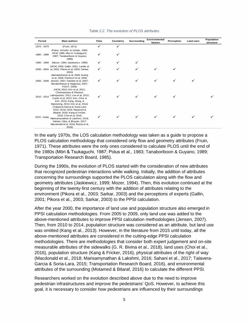
Table 2.2. The evolution of PLOS attributes

Period Main authors Flow Geometry SurroundingEnvironmental

factorsPerception Land uses

Population

structure

1970 - 1979 (Fruin, 1971) ✓ ✓

1980 - 1989

(Polus, Schofer, & Ushpiz, 1983;

HCM, 1985; Mori & Tsukaguchi,

1987; Tanaboriboon & Guyano,

1989)

✓ ✓

1990 - 1999 (Mozer, 1994; Jaskiewicz, 1999) ✓ ✓ ✓

2000 - 2004

(HCM, 2000; Gallin, 2001; Landis et

al, 2001; Pikora et al, 2003; Sarkar,

2003)✓ ✓ ✓ ✓ ✓

2005 - 2009

(Muraleetharan et al, 2005; Ewing

et al, 2006; Petritsch et al, 2006;

Jensen, 2007; Dandan et al, 2007;

Muraleetharan & Hagiwara, 2007;

FDOT, 2009)

✓ ✓ ✓ ✓ ✓ ✓

2010 - 2014

(HCM, 2010; Kim et al, 2011;

Christopoulou & Pitsiava-

Latinopoulou, 2012; Lee et al, 2013;

Carter et al, 2013; Kim, Choi, &

Kim, 2013; Kang, Xiong, &

Mannering, 2013; Kim et al, 2014)

✓ ✓ ✓ ✓ ✓ ✓

2015 - today

(Talavera-Garcia & Soria-Lara,

2015; HCM, 2016; Motamed &

Bitaraf, 2016; Kang & Fricker,

2016; Choi et al, 2016;

Marisamynathan & Lakshmi, 2016;

Sahani, Ojha, & Bhuyan, 2017;

Macdonald et al, 2018; Bivina et al,

2018)

✓ ✓ ✓ ✓ ✓ ✓ ✓

In the early 1970s, the LOS calculation methodology was taken as a guide to propose a

PLOS calculation methodology that considered only flow and geometry attributes (Fruin,

1971). These attributes were the only ones considered to calculate PLOS until the end of

the 1980s (Mōri & Tsukaguchi, 1987; Polus et al., 1983; Tanaboriboon & Guyano, 1989;

Transportation Research Board, 1985).

During the 1990s, the evolution of PLOS started with the consideration of new attributes

that recognized pedestrian interactions while walking. Initially, the addition of attributes

concerning the surroundings supported the PLOS calculation along with the flow and

geometry attributes (Jaskiewicz, 1999; Mozer, 1994). Then, this evolution continued at the

beginning of the twenty-first century with the addition of attributes relating to the

environment (Pikora et al., 2003; Sarkar, 2003) and the perceptions of experts (Gallin,

2001; Pikora et al., 2003; Sarkar, 2003) to the PPSI calculation.

After the year 2000, the importance of land use and population structure also emerged in

PPSI calculation methodologies. From 2005 to 2009, only land use was added to the

above-mentioned attributes to improve PPSI calculation methodologies (Jensen, 2007).

Then, from 2010 to 2014, population structure was considered as an attribute, but land use

was omitted (Kang et al., 2013). However, in the literature from 2015 until today, all the

above-mentioned attributes are considered in the cutting-edge PPSI calculation

methodologies. There are methodologies that consider both expert judgement and on-site

measurable attributes of the sidewalks (G. R. Bivina et al., 2018), land uses (Choi et al.,

2016), population structure (Kang & Fricker, 2016), physical attributes of the right of way

(Macdonald et al., 2018; Marisamynathan & Lakshmi, 2016; Sahani et al., 2017; Talavera-

Garcia & Soria-Lara, 2015; Transportation Research Board, 2016), and environmental

attributes of the surrounding (Motamed & Bitaraf, 2016) to calculate the different PPSI.

Researchers worked on the evolution described above due to the need to improve

pedestrian infrastructures and improve the pedestrians’ QoS. However, to achieve this

goal, it is necessary to consider how pedestrians are influenced by their surroundings

6

when walking (G. R. Bivina et al., 2018; Christopoulou & Pitsiava-Latinopoulou, 2012;

Gallin, 2001; Jaskiewicz, 1999; Pikora et al., 2003; Sarkar, 2003). Nonetheless, it is not

only necessary to consider these influences, but it is also important to revise how

researchers introduced them into the different PPSI methodologies. For this reason, Table

2.3 chronicles the attributes that have been considered to determine the PPSI over time.

7

Table 2.3. Historical review of PPSI methodology attributes

(Author, year) Method Data Country Attributes considered

(Fruin, 1971) Ordinary least

squares regression Video United States Pedestrian density, pedestrian flow; pedestrian space; sidewalk width

(Polus et al., 1983) Ordinary least

squares regression Video Israel Pedestrian density; pedestrian flow; pedestrian space; sidewalk width

(Transportation

Research Board, 1985)

Ordinary least

squares regression Video United States Pedestrian density; pedestrian flow; pedestrian space; sidewalk width

(Mōri & Tsukaguchi,

1987)

Ordinary least

squares regression

Video and

surveys Japan Pedestrian density; pedestrian flow; sidewalk width

(Tanaboriboon &

Guyano, 1989)

Ordinary least

squares regression Video Thailand Pedestrian flow; pedestrian space

(Mozer, 1994) Scoring system Experts

opinion United States

Buffer width; driveways segment; heavy vehicles factor; number of driveways; number of

lanes; pedestrian flow; sidewalk width; vehicular flow; vehicular speed

(Jaskiewicz, 1999) Scoring system Experts


Buffer; building articulation; complexity of spaces; connectivity; enclosure / definition;

lighting; overhangs / awnings / varied roof lines; shade trees; sidewalk condition;

transparency; vehicular speed

(Transportation


Ordinary least

squares regression Video United States Pedestrian flow; pedestrian space; pedestrian speed; sidewalk width

(Gallin, 2001) Scoring system Experts

opinion Australia

Access; buffer width; connectivity; crossing opportunities; mix of path users; number of

driveways; pedestrian flow; security; sidewalk condition; sidewalk width; support facilities

(Landis et al., 2001) Stepwise

regression analysis Survey United States

Bike lane width; buffer width; number of lanes; on street parking segment; outside lane

width; shoulder width; sidewalk width; vehicular flow; vehicular speed

(Pikora et al., 2003) Delphi study Experts

opinion Australia

Amenities; bus stop presence; cleanliness; crossing opportunities; land uses; lighting;

pollution; safety; sidewalk condition; vehicular speed

(Sarkar, 2003) Scoring system Experts


Access; buffer; noise; overhangs / awnings / varied roof lines; pedestrian speed; pollution;

sidewalk condition; sidewalk furniture

8

(Muraleetharan et al.,

2005)

Ordinary least

squares regression

Survey and

expert’s

opinion

Japan

Bike flow opposite direction; bike flow same direction; bike lane width; bike speed; buffer

width; obstructions; on street parking segment; pedestrian flow; pedestrian speed; shoulder

width; sidewalk width

(Ewing, Handy,

Brownson, Clemente,

& Winston, 2006)

Multivariate

statistics

Video and

surveys United States

Comfort; connectivity; enclosure / definition; pedestrian flow; safety; sidewalk width; street

width; transparency; vehicular flow; weather

(Petritsch et al., 2006) Stepwise

regression analysis Survey United States Driveways segment; vehicular flow

(Jensen, 2007) Cumulative logit

regression

Video and

surveys Denmark

Bike flow; buffer width; landscape; land uses; lanes width; median street presence; number

of lanes; on street parking segment; pedestrian flow; sidewalk width; trees presence;

vehicular flow; vehicular speed

(Dandan et al., 2007) Stepwise

regression analysis Survey China Bike flow; buffer width; driveway segment; pedestrian flow; vehicular flow

(Muraleetharan &

Hagiwara, 2007)

Multinomial logit

model Survey Japan

Bike flow opposite direction; bike flow same direction; bike speed; buffer width; crossing

opportunities; obstructions; on street parking segment; pedestrian flow; pedestrian speed;

shoulder width; sidewalk width

(State of Florida

Department of

Transportation, 2009)

Stepwise


Bike lane width; buffer width; number of lanes; on street parking segment; outside lane

width; shoulder width; sidewalk width; vehicular flow; vehicular speed

(Transportation


Stepwise


Bike lane width; buffer; buffer width; number of lanes; on street parking segment; outside

lane width; pedestrian space; shoulder width; sidewalk width; vehicular flow; vehicular

speed

(T. Kim et al., 2011) Multi criteria

decision analysis

Video and

surveys South Korea Landscape; pedestrian flow; sidewalk condition; support facilities

(Christopoulou &

Pitsiava-Latinopoulou,

2012)

Scoring system Survey Greek

Access; buffer; buffer width; bus stop presence; driveways segment; maneuver freedom;

noise; obstructions; pedestrian flow; ramps; safety; sidewalk condition; sidewalk furniture

sidewalk width; trees presence; vehicular flow; vehicular speed

(Lee et al., 2013) Multi criteria

decision analysis Survey South Korea Amenities; connectivity; pedestrian space; pedestrian speed

(Carter et al., 2013) Scoring system Survey United States Buffer; buffer width; lanes width; number of lanes; on street parking segment; sidewalk

length; sidewalk width; vehicular flow; vehicular speed limit

9

(S. Kim et al., 2013) Ordinary least

squares regression Survey South Korea Buffer width; lanes width; sidewalk width; vehicular flow; vehicular speed

(Kang et al., 2013) Ordered

probability model Survey China

Age; amenities; bike flow; bike flow opposite direction; bike flow same direction; bike

speed; buffer; lighting; on street parking segment; pedestrian flow; sidewalk width; weather

(S. S. Kim et al.,

2014)

Ordinary least

squares regression

Video and

surveys South Korea Pedestrian density; pedestrian flow; pedestrian space; pedestrian speed; sidewalk width

(Talavera-Garcia &

Soria-Lara, 2015) Scoring system Survey Spain Amenities; connectivity; sidewalk width; trees presence; vehicular speed

(Transportation


Stepwise


Bike lane width; buffer; buffer width; number of lanes; on street parking segment; outside

lane width; pedestrian space shoulder width; sidewalk width; vehicular flow; vehicular

speed

(Motamed & Bitaraf,

2016) Scoring system

Experts

opinion Iran

Access; amenities; buffer; building articulation; cleanliness; complexity of spaces; crossing

opportunities; driveway segment; land uses; landscape; lighting; noise; number of lanes; on

street parking segment; pollution; public toilet presence; security; sidewalk condition;

sidewalk furniture; sidewalk width; trees presence; vehicular flow; vehicular speed

(Kang & Fricker,

2016)

Ordered

probability model

Video and

surveys China

Age; bike flow; bike speed; buffer; genre; household size; marital status; number of lanes;

pedestrian flow; pedestrian speed; sidewalk width; trees presence; weather

(Choi et al., 2016) Ordered

probability model Survey South Korea

Bike lane presence; bus stop presence; crossing opportunities; driveways segment; land

uses; median street presence; number of lanes; pedestrian flow; sidewalk width; trees

presence

(Marisamynathan &

Lakshmi, 2016)

Stepwise

regression analysis

Video and

surveys India Buffer; sidewalk condition; sidewalk width; vehicular flow

(Sahani et al., 2017) Stepwise

regression analysis Survey India

Bike flow; bike lane width; buffer width; obstructions; on street parking segment; peddlers’

segment; sidewalk width; vehicular flow; vehicular speed

(Macdonald et al.,

2018) Scoring system

Experts


Access; buffer; building articulation; crossing opportunities; enclosure; number of lanes;

shade trees; sidewalk width; transparency

(G. R. Bivina et al.,

2018) Scoring system Survey India

Access; buffer; cleanliness; comfort; crossing opportunities; obstructions; security;

sidewalk condition; sidewalk width

(Geetha Rajendran

Bivina & Parida,

2019)

Structural Equation

Modelling Survey India

Access, amenities, bus stop presence cleanliness, lighting, obstructions, pedestrian flow,

security, sidewalk condition, sidewalk continuity, sidewalk width, vehicular flow, vehicular

speed

10

The attributes considered for the first attempt at PLOS calculation were pedestrian density

and space, these being very similar to the attributes considered to calculate motor

vehicles’ LOS. The idea behind the use of these attributes considered that there would be

a positive correlation between the pedestrian’s space and the PLOS. This means that if

there were more space for a pedestrian to use, the PLOS of that sidewalk also improved.

Similarly, the correlation between the PLOS and pedestrian density was considered

negative. This is because with high densities, the crowd that formed would impact the

PLOS in a negative way (Fruin, 1971; Mōri & Tsukaguchi, 1987; Polus et al., 1983;

Tanaboriboon & Guyano, 1989; Transportation Research Board, 1985).

Over the following years, some researchers started to include other attributes to calculate

the PPSI besides those already considered. For example, the inclusion of pedestrian

speed was considered as an important attribute for PPSI calculation because of the idea of

these times about the pedestrians’ need to complete their trips quickly (Muraleetharan et

al., 2005; Muraleetharan & Hagiwara, 2007; Transportation Research Board, 2000).

Similarly, attributes that consider the interaction with other modes that might affect the

pedestrians’ trips like the buffer width, vehicular flow, vehicular speed, number of vehicular

lanes, driveways, and the heavy goods vehicle (HGV) factor were also considered (Mozer,

1994).

However, during the same period, a theory also emerged that considered pedestrian

interaction with the surroundings when walking in three different aspects: architectural,

amenities, and road safety. The architectural aspect considered the provision of good

spaces for pedestrians on the sidewalk in terms of space definition, connectivity, and

friendly facades (non-continuous) to generate a positive PPSI. Similarly, for the amenities

aspects, the literature considered that providing shade from trees, facades with

transparent areas, and good sidewalk conditions were important to provide a good PPSI.

Finally, this theory also considered road safety in the generation of a good PPSI with the

inclusion of the buffer and vehicular speed attributes (Jaskiewicz, 1999).

The advancing methodologies included new attributes that allowed for an understanding of

pedestrian needs and feelings with more accuracy using environmental attributes and

expert judgement. In general, the attributes did not change, instead, the way of

understanding these attributes was modified by the consideration of pedestrians and

expert perceptions of each of them (Gallin, 2001; Landis et al., 2001; Pikora et al., 2003).

Nonetheless, with the consideration of environmental attributes, new attributes that might

influence the PPSI like pollution, noise, and lighting were considered (Pikora et al., 2003;

Sarkar, 2003). However, these attributes stopped being considered in the literature related

with pedestrian service indicators for around ten years until they were reintroduced in the

2010s (Christopoulou & Pitsiava-Latinopoulou, 2012; Kang et al., 2013; Motamed &

Bitaraf, 2016).

Some studies started to consider pedestrian interaction with other transport modes where

authors focused on the interaction that pedestrians may have with bicycles on the sidewalk

and how these interactions may negatively impact the PPSI (Dandan et al., 2007; Jensen,

2007; Muraleetharan et al., 2005; Muraleetharan & Hagiwara, 2007; State of Florida

Department of Transportation, 2009). In addition, the interaction between pedestrians and

other transportation modes using the adjacent transportation infrastructure was also

considered to negatively impact walking activity (D. A. Rodríguez, Aytur, Forsyth, Oakes, &

11

Clifton, 2008) and the PPSI (Dandan et al., 2007; Ewing et al., 2006; Jensen, 2007;

Muraleetharan & Hagiwara, 2007; Petritsch et al., 2006; State of Florida Department of

Transportation, 2009). However, one of the most relevant aspects in understanding the

PPSI was the inclusion of the term “comfort” to the attributes mentioned above (Ewing et

al., 2006; Landis et al., 2001; Mōri & Tsukaguchi, 1987).

In the vanguard literature there are few changes to PPSI calculation methodologies.

Chiefly, the main attributes considered over time are also considered in the most recent

period (G. R. Bivina et al., 2018; Carter et al., 2013; Choi et al., 2016; S. Kim et al., 2013;

S. S. Kim et al., 2014; T. Kim et al., 2011; Lee et al., 2013; Macdonald et al., 2018;

Marisamynathan & Lakshmi, 2016; Sahani et al., 2017; Talavera-Garcia & Soria-Lara,

2015; Transportation Research Board, 2010, 2016). Additionally, nowadays, the use of the

term “comfort” is also considered (G. R. Bivina et al., 2018; Dandan et al., 2007; Kang et

al., 2013; Marisamynathan & Lakshmi, 2016). One of the most notable inclusions was the

use of population structure data (i.e., age, sex, marital status, and household size) to

characterize pedestrians and the way that these pedestrian groups perceive the PPSI

(Kang & Fricker, 2016; Kang et al., 2013). In other studies, a new line of research was also

developed where an understanding of how the design of walkable areas contributes to the

perception of QoS using stated preferences from image-based experiments (Adkins, Dill,

Luhr, & Neal, 2012; Borst, Miedema, de Vries, Graham, & van Dongen, 2008; Ewing &

Handy, 2009; Hurtubia, Guevara, & Donoso, 2015).

Up to this point in the chapter, the literature has been presented from the researcher’s

perspective, concentrating on the evolution of the PPSI. This due to the fact that there is

not much information about how pedestrians perceive and understand the PPSI. Geetha

Rajendran Bivina & Parida (2019) proposed a structural equation modelling (SEM)

approach to explain the influence that the built environment has on the perceived PLOS in

India. This approach was based on pedestrian perceptions and found four latent variables

(safety, security, mobility, and infrastructure, and comfort and convenience) that positively

impacted the perceived PLOS (Geetha Rajendran Bivina & Parida, 2019). However, there

are not many studies that consider pedestrian perception of the QoS and the negative

impacts that can be generated on this QoS from subjective attributes (e.g., perceptions).

For this reason, it is necessary to expand on the knowledge of this topic by considering the

sidewalk users’ point of view. This consideration has been taken into account in other

transportation areas, where the inclusion of users’ perceptions improves the models’

performance (Fernández-Heredia et al., 2016). For this reason, based on the literature and

the satisfaction theories contained within, a structure of how pedestrians perceive and

understand the PPSI will be hypothesized.

It has been established in the literature on satisfaction theories that there are direct and

positive effects generated on the user’s satisfaction from their perceived QoS. In addition,

it has also been proven that users’ perceptions of the different elements with which they

interact positively or negatively impacts their walking activity (Schwartz, Aytur, Evenson, &

Rodríguez, 2009) and their perception of the QoS (Aliman, Hashim, Wahid, & Harudin,

2016; Badara et al., 2013; Nilplub, Khang, & Krairit, 2016; Subramanian, Gunasekaran,

Yu, Cheng, & Ning, 2014). These interactions can result in positive or negative effects on

the perceived QoS and user’s satisfaction. Considering these effects and the

12

methodologies previously described, a structure of how pedestrians perceive their PPSI is

proposed in Figure 2.1.

Figure 2.1. Proposed structure of pedestrians’ perceived QoS

As Figure 2.1 sets out, an understanding of the perceived QoS is the base on which later

understanding other effects on PPSIs is built. Pedestrian QoS can be influenced positively

and negatively depending on the interaction between the pedestrian and the sidewalk. For

example, there is much evidence supporting the fact that the sidewalk characteristics

positively impact the pedestrians’ PPSIs (e.g., sidewalk width, sidewalk condition,

furniture, trees, public transport access, and signage) (Asadi-Shekari, Moeinaddini, & Zaly

Shah, 2013; Banerjee, Maurya, & Lämmel, 2018). In addition, there are also surroundings

characteristics like the weather (Ewing et al., 2006; Kang & Fricker, 2016; Kang et al.,

2013), lighting (Jaskiewicz, 1999; Kang et al., 2013; Motamed & Bitaraf, 2016; Pikora et

al., 2003), cleanliness (G. R. Bivina et al., 2018; Motamed & Bitaraf, 2016; Pikora et al.,

2003), and landscape (T. Kim et al., 2011; Motamed & Bitaraf, 2016) that positively impact

the pedestrians’ QoS perceptions. Also, the protection that pedestrians perceive in terms

of safety (Christopoulou & Pitsiava-Latinopoulou, 2012; Pikora et al., 2003) and security

(G. R. Bivina et al., 2018; Gallin, 2001; Motamed & Bitaraf, 2016; Villaveces Dr. et al.,

2012) positively impacts the PPSI and how pedestrians perceive the QoS. Finally, it has

also been found that providing good amenities for pedestrians like public restrooms

(Motamed & Bitaraf, 2016), shops (Jensen, 2007; Motamed & Bitaraf, 2016; Pikora et al.,

2003), and shade (Jaskiewicz, 1999; Macdonald et al., 2018) also positively impacts their

perception of QoS.

On the other hand, there are also some sidewalk attributes related to pedestrian

interactions that negatively impact the different PPSIs. For example, the discomfort that

pedestrians feel when they interact with other pedestrians negatively impacts the

pedestrian perception of QoS (G. R. Bivina et al., 2018; Christopoulou & Pitsiava-

Latinopoulou, 2012; Muraleetharan et al., 2005; Muraleetharan & Hagiwara, 2007; Sahani

et al., 2017). Similarly, the effects that produce on pedestrians the motor vehicles

(externalities) like the HGV flow (Mozer, 1994), vehicular speed (Christopoulou & Pitsiava-

Latinopoulou, 2012; Jaskiewicz, 1999; Jensen, 2007; S. Kim et al., 2013; Landis et al.,

2001; Motamed & Bitaraf, 2016; Mozer, 1994; Pikora et al., 2003; Sahani et al., 2017;

State of Florida Department of Transportation, 2009; Talavera-Garcia & Soria-Lara, 2015;

Transportation Research Board, 2010, 2016), noise (Christopoulou & Pitsiava-

Latinopoulou, 2012; Motamed & Bitaraf, 2016; Sarkar, 2003), pollution (Motamed &

Bitaraf, 2016; Pikora et al., 2003; Sarkar, 2003), and some characteristics of the vehicular

transportation infrastructure like road width (Carter et al., 2013; Jensen, 2007; S. Kim et

al., 2013) and the number of vehicular lanes (Carter et al., 2013; Choi et al., 2016; Jensen,

13

2007; Kang & Fricker, 2016; Macdonald et al., 2018; Motamed & Bitaraf, 2016; Mozer,

1994; State of Florida Department of Transportation, 2009; Transportation Research

Board, 2010, 2016) also negatively impact the PPSI and the pedestrians’ perception of the

QoS. Finally, the interaction of pedestrians with bicyclists in terms of bicycle flow (Dandan

et al., 2007; Jensen, 2007; Kang & Fricker, 2016; Kang et al., 2013; Muraleetharan et al.,

2005; Muraleetharan & Hagiwara, 2007; Sahani et al., 2017) and speed (Kang & Fricker,

2016; Kang et al., 2013; Muraleetharan et al., 2005; Muraleetharan & Hagiwara, 2007)

also negatively impacts their perception of QoS.

The different attributes affecting pedestrians’ perceived PPSI have been identified from the

literature review. It has been common practice to use objective and subjective attributes

independently of each other to understand and calculate the different PPSI. However,

there is no clear quantification of how much the users’ perceptions impact the perceived

QoS. In addition, there are few studies that consider pedestrian perceptions of their

sensorial experience when walking to explain the pedestrian’s perceived QoS. Geetha

Rajendran Bivina & Parida (2019) found that there are four latent variables that positively

affect the PLOS. However, latent variables that negatively impact the pedestrian

perception of the QoS were not found in the literature. In addition, there are no

methodologies that consider the interaction of pedestrian and the infrastructure to provide

a PPSI calculation. These gaps will be addressed in this study by expanding on existing

knowledge about the role of perceptions in the explanation and calculation of quality of

service.

14

3. Methodology

The aim of this study is to examine how and to what extent the pedestrian sensorial walking experience on urban sidewalks explains pedestrian perceptions of the QoS. To fulfill it, a literature review was conducted to identify the main attributes and methodologies related to PPSI calculation and pedestrian QoS. Then, based on the literature review, 1056 interception surveys were applied in Bogotá, asking pedestrians about their perceptions of sidewalk attributes. To quantify the contribution of the perception of sidewalk attributes to the explanation of the perceived QoS, initially, OLS models were estimated by combining groups of independent variables (environmental, sociodemographic, physical, and perceptual). Then, to understand how pedestrians perceived the QoS, a QoS pedestrian cognitive map using a SEM approach was proposed. Finally, to predict the perceived QoS and sidewalk QoS (SQoS) using pedestrians’ perceptions, four different approaches were used (OLS, ordered probit, continuous MIMIC, and ordered probit MIMIC), and the best one for each case was

selected by considering the match score, error variability, and 𝜒2 values. This chapter outlines the methodology that was followed to carry out each of these processes.

3.1 Literature review process

To identify attributes that affect pedestrian QoS when walking, as well as the methodologies available for the prediction of different PPSI, a four-step literature review was developed (Figure 3.1). In step 1, four databases (Web of Science ®, SCOPUS ®, ASCE ® and EBSCOhost ®) in which relevant articles would be searched for were selected. Step 2 identified the most relevant keywords related to pedestrians and the QoS rating (pedestrian, sidewalk, level of service, quality of service, comfort, satisfaction, pleasure, and stress). These terms were combined using as a base terms “pedestrian” and “sidewalk” and adding the terms “level of service”, “quality of service”, “comfort”, “satisfaction”, “pleasure”, and “stress”. In step 3 the search was limited in terms of time period from 1950 to 2019 and by topic where only relevant articles related to urban sidewalks were considered. Finally, step 4 identified the different attributes and main methodologies related to PPSI and its calculation. In some cases, relevant literature was also identified within the references of each of the studied papers as well as by considering advisors’ and evaluators’ recommendations.

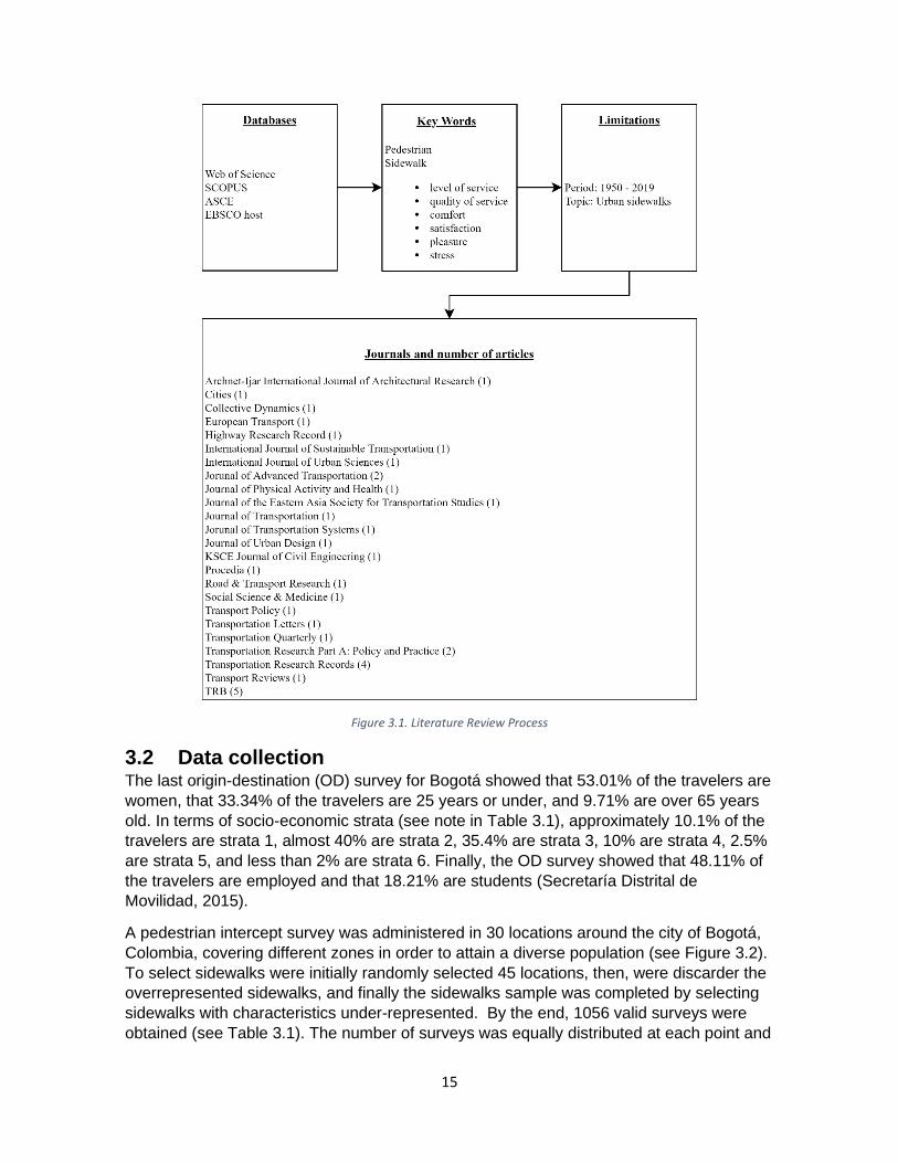
15

Figure 3.1. Literature Review Process

3.2 Data collection The last origin-destination (OD) survey for Bogotá showed that 53.01% of the travelers are

women, that 33.34% of the travelers are 25 years or under, and 9.71% are over 65 years

old. In terms of socio-economic strata (see note in Table 3.1), approximately 10.1% of the

travelers are strata 1, almost 40% are strata 2, 35.4% are strata 3, 10% are strata 4, 2.5%

are strata 5, and less than 2% are strata 6. Finally, the OD survey showed that 48.11% of

the travelers are employed and that 18.21% are students (Secretaría Distrital de

Movilidad, 2015).

A pedestrian intercept survey was administered in 30 locations around the city of Bogotá,

Colombia, covering different zones in order to attain a diverse population (see Figure 3.2).

To select sidewalks were initially randomly selected 45 locations, then, were discarder the

overrepresented sidewalks, and finally the sidewalks sample was completed by selecting

sidewalks with characteristics under-represented. By the end, 1056 valid surveys were

obtained (see Table 3.1). The number of surveys was equally distributed at each point and

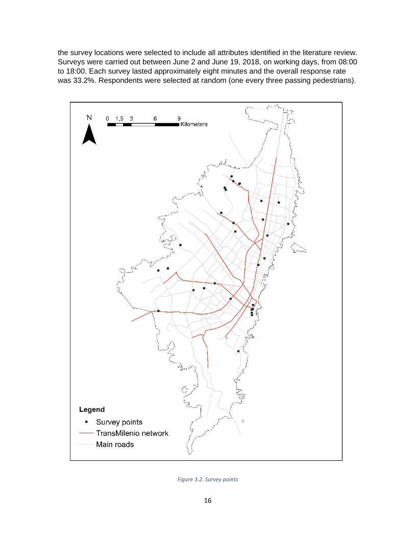
16

the survey locations were selected to include all attributes identified in the literature review.

Surveys were carried out between June 2 and June 19, 2018, on working days, from 08:00

to 18:00. Each survey lasted approximately eight minutes and the overall response rate

was 33.2%. Respondents were selected at random (one every three passing pedestrians).

Figure 3.2. Survey points

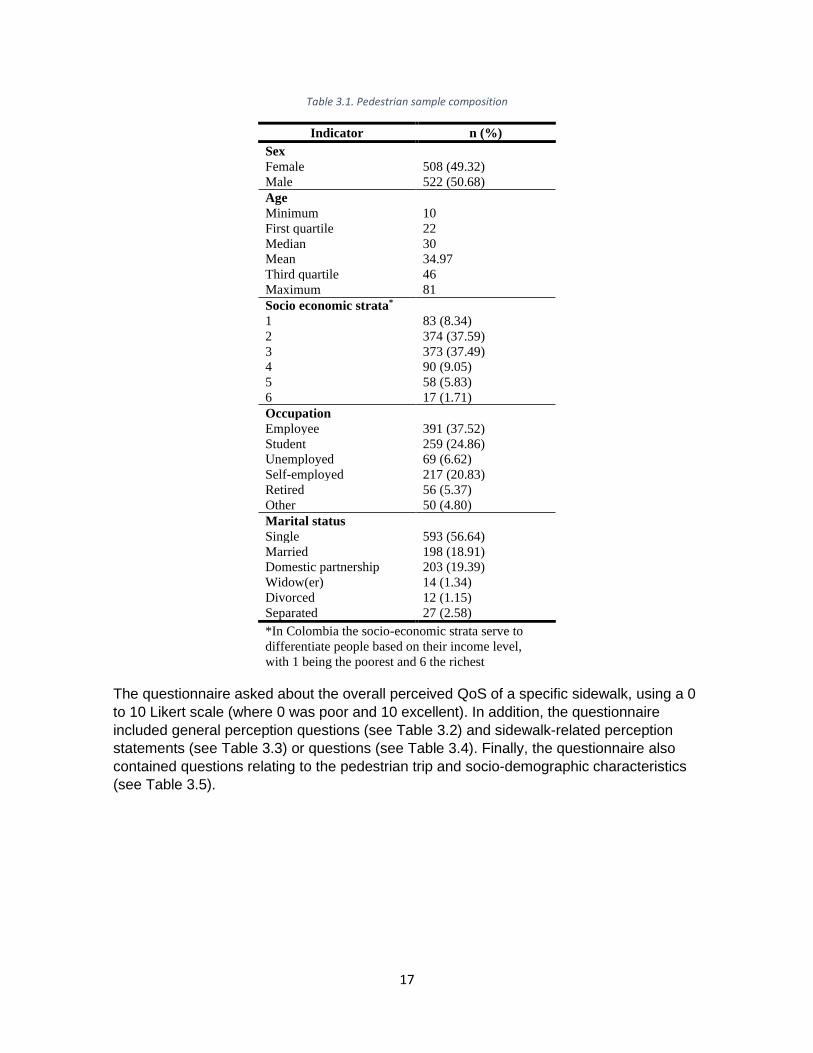
17

Table 3.1. Pedestrian sample composition

Indicator n (%)

Sex

Female 508 (49.32)

Male 522 (50.68)

Age

Minimum 10

First quartile 22

Median 30

Mean 34.97

Third quartile 46

Maximum 81

Socio economic strata*

1 83 (8.34)

2 374 (37.59)

3 373 (37.49)

4 90 (9.05)

5 58 (5.83)

6 17 (1.71)

Occupation

Employee 391 (37.52)

Student 259 (24.86)

Unemployed 69 (6.62)

Self-employed 217 (20.83)

Retired 56 (5.37)

Other 50 (4.80)

Marital status

Single 593 (56.64)

Married 198 (18.91)

Domestic partnership 203 (19.39)

Widow(er) 14 (1.34)

Divorced 12 (1.15)

Separated 27 (2.58)

*In Colombia the socio-economic strata serve to

differentiate people based on their income level,

with 1 being the poorest and 6 the richest

The questionnaire asked about the overall perceived QoS of a specific sidewalk, using a 0

to 10 Likert scale (where 0 was poor and 10 excellent). In addition, the questionnaire

included general perception questions (see Table 3.2) and sidewalk-related perception

statements (see Table 3.3) or questions (see Table 3.4). Finally, the questionnaire also

contained questions relating to the pedestrian trip and socio-demographic characteristics

(see Table 3.5).

18

Table 3.2. General perception questions

Variable Statement/Question Range

Pedestrians

Rate, from 0 to 10, how comfortable would you find the general

presence of the following when walking:

0 – 10

Restrooms

Shops

Shade

Street vendors

Bike flow

Rate, from 0 to 10, how bothering would you find the presence

of the following when walking on the sidewalk:

Bike speed

Opposite direction flow

Same direction flow

Obstructions

Table 3.3. Sidewalk-related statements


Where 0 is totally disagree and 10 totally agree, rate from 0 to 10 the following statements:

Pedestrians far

away from me

When walking on this sidewalk, I prefer other pedestrians to be

far away from me

0 – 10

Stress Walking on this sidewalk is stressful

Too many

pedestrians

On this sidewalk, the number of pedestrians does not let me

walk freely

Vehicular flow

too close On this sidewalk the motor vehicle flow is too close to me

I prefer not to

walk here I would rather not walk on this sidewalk

Crossing the

street is easy On this sidewalk it is easy to cross to the other side

Accessibility On this sidewalk it is easy to walk with a stroller or wheelchair

Connectivity To take today’s walk I could use another route

Order This sidewalk is orderly

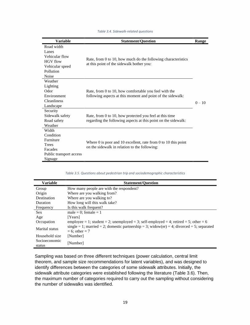
19

Table 3.4. Sidewalk-related questions


Road width

Rate, from 0 to 10, how much do the following characteristics

at this point of the sidewalk bother you:

0 – 10

Lanes

Vehicular flow

HGV flow

Vehicular speed

Pollution

Noise

Weather

Rate, from 0 to 10, how comfortable you feel with the

following aspects at this moment and point of the sidewalk:

Lighting

Odor

Environment

Cleanliness

Landscape

Security

Rate, from 0 to 10, how protected you feel at this time

regarding the following aspects at this point on the sidewalk:

Sidewalk safety

Road safety

Weather

Width

Where 0 is poor and 10 excellent, rate from 0 to 10 this point

on the sidewalk in relation to the following:

Condition

Furniture

Trees

Facades

Public transport access

Signage

Table 3.5. Questions about pedestrian trip and sociodemographic characteristics

Variable Statement/Question

Group How many people are with the respondent?

Origin Where are you walking from?

Destination Where are you walking to?

Duration How long will this walk take?

Frequency Is this walk frequent?

Sex male = 0; female = 1

Age [Years]

Occupation employee = 1; student = 2; unemployed = 3; self-employed = 4; retired = 5; other = 6

Marital status single = 1; married = 2; domestic partnership = 3; widow(er) = 4; divorced = 5; separated

= 6; other = 7

Household size [Number]

Socioeconomic

status [Number]

Sampling was based on three different techniques (power calculation, central limit

theorem, and sample size recommendations for latent variables), and was designed to

identify differences between the categories of some sidewalk attributes. Initially, the

sidewalk attribute categories were established following the literature (Table 3.6). Then,

the maximum number of categories required to carry out the sampling without considering

the number of sidewalks was identified.

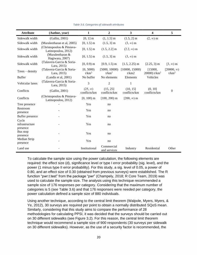
20

Table 3.6. Categories of sidewalk attributes

Attribute (Author, year) 1 2 3 4 5

Sidewalk width (Gallin, 2001) [0, 1] m (1, 1.5] m (1.5, 2] m (2, ∞) m

Sidewalk width (Muraleetharan et al, 2005) [0, 1.5] m (1.5, 3] m (3, ∞) m

Sidewalk width (Christopoulou & Pitsiava-

Latinopoulou, 2012) [0, 1.5] m (1.5, 2.2] m (2.2, ∞) m

Sidewalk width (Muraleetharan &

Hagiwara, 2007) [0, 1.5] m (1.5, 3] m (3, ∞) m

Sidewalk width (Talavera-Garcia & Soria-

Lara, 2015) [0, 0.9) m [0.9, 1.5) m [1.5, 2.25) m [2.25, 3) m [3, ∞) m

Trees – density (Talavera-Garcia & Soria-

Lara, 2015)

[0, 5000)

t/km2

[5000, 10000)

t/km2

[10000, 15000)

t/km2

[15000,

20000) t/km2

[20000, ∞)

t/km2

Buffer (Landis et al, 2001) No buffer No elements Elements Vehicles

Vehicular lanes (Talavera-Garcia & Soria-

Lara, 2015) 3 2 1

Conflicts (Gallin, 2001) (25, ∞)

conflicts/km

(15, 25]

conflicts/km

(10, 15]

conflicts/km

(0, 10]

conflicts/km 0

Conflicts (Christopoulou & Pitsiava-

Latinopoulou, 2012) [0, 100) m [100, 200) m [200, ∞) m

Tree presence - Yes no

Restroom

presence - Yes no

Buffer presence - Yes no

Cycle

infrastructure

presence

- Yes no

Bus stop

presence - Yes no

Median Strip

presence - Yes no

Land use - Institutional Commercial

and services Industry Residential Other

To calculate the sample size using the power calculation, the following elements are

required: the effect size (d), significance level or type I error probability (sig. level), and the

power (1 minus type II error probability). For this study, a sig. level of 0.05, a power of

0.80, and an effect size of 0.30 (obtained from previous surveys) were established. The R

function “pwr.t.test” from the package “pwr” (Champely, 2018; R Core Team, 2019) was

used to calculate the sample size. The analysis using this technique recommended a

sample size of 176 responses per category. Considering that the maximum number of

categories is 5 (see Table 3.6) and that 176 responses were needed per category, the

power calculation defined a sample size of 880 individuals.

Using another technique, according to the central limit theorem (Walpole, Myers, Myers, &

Ye, 2012), 30 surveys are required per point to obtain a normally distributed SQoS mean.

Similarly, considering that this study aims to compare the performance of 28

methodologies for calculating PPSI, it was decided that the surveys should be carried out

on 30 different sidewalks (see Figure 3.2). For this reason, the central limit theorem

technique would recommend a sample size of 900 respondents (30 surveys per sidewalk

on 30 different sidewalks). However, as the use of a security factor is recommended, the

21

decision was made to administer five additional surveys on each sidewalk, generating a

sample size of 1050 surveys.

Finally, using the sample size recommendations for studies that use latent variables in a

conservative way, the decision was made to use a sample size of 20 times the number of

variables (Mundfrom, Shaw, & Ke, 2005). As there are 43 independent variables in the

questionnaire (see Table 3.2, Table 3.3, and Table 3.4) a sample size of 860 was

calculated. In spite that the three techniques previously mentioned are used to meet

different needs (e.g., power analysis to have enough power to detect associations, central

limit theorem to have enough power to make inferences about the population mean), a

sample size of 1050 respondents was chosen, using the result of the central limit theorem

technique as it produced the largest sample size.

Sidewalk selection made sure to cover all previously identified categories (see Table 3.6).

Initially, 45 random locations in Bogotá were selected. Then, each one was visited and

sidewalk information was collected about the objective on-site attributes identified in the

pedestrian QoS literature (see Table 3.7). From this data collection process, sidewalks

comprising a variety of attributes were selected and sidewalk that overrepresent the

characteristics were discarded. Then, sidewalks with characteristics that were not present

in the initially selected sidewalks were chosen to complete the sample of 30 sidewalks.

The different characteristics and a sample image of each sidewalk can be seen in

Appendix A – Sidewalk sample.

Table 3.7. Sidewalk on-site measurable attributes

Attribute Units Attribute Units

Sidewalk width [m] Lanes width [m]

Sidewalk length [m] Road width [m]

Trees [Number] Shoulder width [m]

Lanes [Number] Bicycle infrastructure width [m]

Conflicts [Number] Driveway length [m]

Restrooms [Number] Transparent panel length [m]

Median strip [yes=1; no=0] Roof length [m]

Buffer width [m] Sidewalk entrances [Number]

Buffer presence [yes=1; no=0] Driveways [Number]

Land use [see Table 3.6] Ramps [Number]

Speed limit [km/h] Facade separation [m]

Exterior lane width [m]

Once the 30 sidewalks were selected, a team visited them to collect all the data needed.

The team was composed of four surveyors and one technician who worked eight hours per

day during working days. On each sidewalk, specific assignments were assigned to each

member of the team to collect the data required by the survey (see Table 3.2, Table 3.3,

Table 3.4, and Table 3.5) and also the objective on-site variable attributes (see Table 3.8).

22

Table 3.8. Sidewalk on-site variable attributes

Attribute Period/Units Attribute Period/Units

Bicycle flow on road [5 min] Other flow on sidewalk [5 min]

Motorcycle flow [5 min] Vehicular speed [km/h]

Vehicular flow [5 min] Noise [dB]

Bus flow [5 min] Temperature [°C]

HGV flow [5 min] Lighting [lux]

Pedestrian flow [5 min] Humidity [% Hr]

Bicycle flow on sidewalk [5 min] On-street parking [Number]

3.3 Modelling approach Five different models were considered in the specification searches of this study. OLS and

ordered probit models are a common choice to study the influence of independent

variables on a specific dependent variable (which for this study is the perceived QoS).

Structural equation models (SEM) and multiple indicator and multiple cause (MIMIC)

models are commonly used to test the existence of latent variables from perception

attributes that, in the case of MIMIC models, can be forecasted or explained by objective

attributes. Finally, the multi-attribute utility theory (MAUT) is normally used to define a

ranking by comparing the results of certain characteristics of different options.

3.3.1. Ordinary least squares (OLS) models The OLS model presented in Equation (1) is used to quantify the contribution of perception

attributes to the explanation of perceived QoS. In addition, this model is one of the options

for the proposition of a forecasting model of the perceived SQoS and QoS. It is commonly

used for its simplicity in estimating a linear equation to explain a dependent variable (y) on

the basis of a set of independent variables (xi). OLS models assume independence between

the independent variables and homoscedasticity (Ortúzar & Willumsen, 2011, Section

4.2.1).

𝑦 = 𝛽0 +∑𝛽𝑖 ∗ 𝑥𝑖

𝑛

𝑖=1

+ 𝜀 (1)

The OLS models can quantify the proportion of variation in the data explained by the

model. In fact, the coefficient of determination (R2) is defined as the ratio between the

explained variation and the total variation (Ortúzar & Willumsen, 2011, page 150), and can

be calculated using Equation (2):

𝑅2 =∑ (𝑌�̂� − �̅�)

2𝑛𝑖=1

∑ (𝑌𝑖 − �̅�)2𝑛

𝑖=1

(2)

The R2 value increases with the inclusion of more independent variables. For this reason,

the adjusted R2 was developed to correct for this problem. The adjusted R2 can be

calculated using Equation (3):

23

𝑎𝑑𝑗 𝑅2 = (𝑅2 −𝑘

𝑛 − 1) ∗ (

𝑛 − 1

𝑛 − 𝑘 − 1) (3)

where n is the sample size and k the number of independent variables.

In addition, to test if all coefficients of the OLS models are significantly different from zero,

an F-test was calculated for the complete model. Using this test, the null hypothesis (H0)

poses that all coefficients are equal to 0 (𝐻0: (𝛽0, 𝛽𝑖) = 0). In this case, H0 is accepted if the

F-test value is less than or equal to the F critical value (Ortúzar & Willumsen, 2011, page

151).

3.3.2. Ordered probit models

Ordered probit models are an appropriate approach for choice modeling with discrete and

ordered nature data (Harvey & Amemiya, 2006; Washington, Karlaftis, & Mannering,

2010). To use this model, an unobserved variable z is defined usually as a linear function

of each observation: (see Equation (4))

𝑧 = 𝛽𝑋 + 𝜀 (4)

where X is a vector of variables determining the observations’ order, 𝛽 a vector of

parameters, and 𝜀 a random disturbance. This model assumes that all parameters 𝛽 are

the same for the different ordered categories. Using Equation (4), the observed ordered

data (y) for each observation is defined by taking Equation (5) into consideration

(Washington et al., 2010).

𝑦 = 1 𝑖𝑓 𝑧 ≤ 𝜇0

𝑦 = 2 𝑖𝑓 𝜇0 < 𝑧 ≤ 𝜇1

𝑦 = 3 𝑖𝑓 𝜇1 < 𝑧 ≤ 𝜇2

𝑦 = ⋯

𝑦 = 𝐼 𝑖𝑓 𝑧 ≥ 𝜇𝐼−1

(5)

where 𝜇𝑖 are estimated thresholds that define y, and “I” is the highest integer ordered

response. If the random disturbance is assumed to be independent and normally

distributed with mean 0 and variance 1, the probabilities for the ordered probit model can

be calculated using Equation (6):

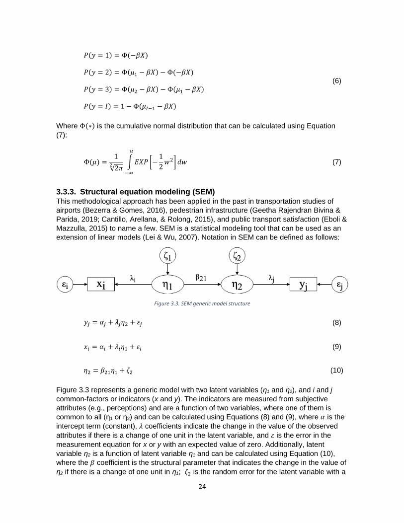
24

𝑃(𝑦 = 1) = Φ(−𝛽𝑋)

𝑃(𝑦 = 2) = Φ(𝜇1 − 𝛽𝑋) − Φ(−𝛽𝑋)

𝑃(𝑦 = 3) = Φ(𝜇2 − 𝛽𝑋) − Φ(𝜇1 − 𝛽𝑋)

𝑃(𝑦 = 𝐼) = 1 −Φ(𝜇𝐼−1 − 𝛽𝑋)

(6)

Where Φ(∗) is the cumulative normal distribution that can be calculated using Equation

(7):

Φ(𝜇) =1

√2𝜋2 ∫𝐸𝑋𝑃 [−

1

2𝑤2] 𝑑𝑤

𝑢

−∞

(7)

3.3.3. Structural equation modeling (SEM) This methodological approach has been applied in the past in transportation studies of

airports (Bezerra & Gomes, 2016), pedestrian infrastructure (Geetha Rajendran Bivina &

Parida, 2019; Cantillo, Arellana, & Rolong, 2015), and public transport satisfaction (Eboli &

Mazzulla, 2015) to name a few. SEM is a statistical modeling tool that can be used as an

extension of linear models (Lei & Wu, 2007). Notation in SEM can be defined as follows:

Figure 3.3. SEM generic model structure

𝑦𝑗 = 𝛼𝑗 + 𝜆𝑗𝜂2 + 𝜀𝑗 (8)

𝑥𝑖 = 𝛼𝑖 + 𝜆𝑖𝜂1 + 𝜀𝑖 (9)

𝜂2 = 𝛽21𝜂1 + 𝜁2 (10)

Figure 3.3 represents a generic model with two latent variables (η1 and η2), and i and j

common-factors or indicators (x and y). The indicators are measured from subjective

attributes (e.g., perceptions) and are a function of two variables, where one of them is

common to all (η1 or η2) and can be calculated using Equations (8) and (9), where 𝛼 is the

intercept term (constant), 𝜆 coefficients indicate the change in the value of the observed

attributes if there is a change of one unit in the latent variable, and 𝜀 is the error in the

measurement equation for x or y with an expected value of zero. Additionally, latent

variable η2 is a function of latent variable η1 and can be calculated using Equation (10),

where the 𝛽 coefficient is the structural parameter that indicates the change in the value of

η2 if there is a change of one unit in η1; 𝜁2 is the random error for the latent variable with a

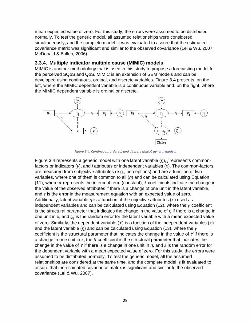
25

mean expected value of zero. For this study, the errors were assumed to be distributed

normally. To test the generic model, all assumed relationships were considered

simultaneously, and the complete model fit was evaluated to assure that the estimated

covariance matrix was significant and similar to the observed covariance (Lei & Wu, 2007;

McDonald & Bollen, 2006).

3.3.4. Multiple indicator multiple cause (MIMIC) models MIMIC is another methodology that is used in this study to propose a forecasting model for

the perceived SQoS and QoS. MIMIC is an extension of SEM models and can be

developed using continuous, ordinal, and discrete variables. Figure 3.4 presents, on the

left, where the MIMIC dependent variable is a continuous variable and, on the right, where

the MIMIC dependent variable is ordinal or discrete.

Figure 3.4. Continuous, ordered, and discrete MIMIC general models

Figure 3.4 represents a generic model with one latent variable (η), j represents common-

factors or indicators (y), and i attributes or independent variables (x). The common-factors

are measured from subjective attributes (e.g., perceptions) and are a function of two

variables, where one of them is common to all (η) and can be calculated using Equation

(11), where 𝛼 represents the intercept term (constant), 𝜆 coefficients indicate the change in

the value of the observed attributes if there is a change of one unit in the latent variable,

and 𝜀 is the error in the measurement equation with an expected value of zero.

Additionally, latent variable η is a function of the objective attributes (xi) used as

independent variables and can be calculated using Equation (12), where the 𝛾 coefficient

is the structural parameter that indicates the change in the value of η if there is a change in

one unit in x, and 𝜁𝜂 is the random error for the latent variable with a mean expected value

of zero. Similarly, the dependent variable (Y) is a function of the independent variables (xi)

and the latent variable (η) and can be calculated using Equation (13), where the 𝛾

coefficient is the structural parameter that indicates the change in the value of Y if there is

a change in one unit in x, the 𝛽 coefficient is the structural parameter that indicates the

change in the value of Y if there is a change in one unit in η, and 𝜀 is the random error for

the dependent variable with a mean expected value of zero. For this study, the errors were

assumed to be distributed normally. To test the generic model, all the assumed

relationships are considered at the same time, and the complete model is fit evaluated to

assure that the estimated covariance matrix is significant and similar to the observed

covariance (Lei & Wu, 2007).

26

𝑦𝑗 = 𝛼𝑗 + 𝜆𝑗𝜂 + 𝜀𝑗 (11)

𝜂 = 𝛾𝑖𝑥𝑖 + 𝜁𝜂 (12)

𝑌 = 𝛾𝑖𝑥𝑖 + 𝛽𝜂 + 𝜀 (13)

Forecasting using MIMIC requires estimating a complete model composed by the

measurement model and the structural model (attributes and indicators). For this reason,

to build a forecasting model the following steps were carried out:

1. The development of the best fit SEM model using only perception attributes

(measurement and structural model)

2. The prediction of the dependent variable (service quality) and all latent variables of

the best fit model using on-site measurables attributes

3. The inclusion of the on-site measurable attributes with a p-value lower than 0.10

using a forward iteration approach (introducing the attributes with a lower p-value

and greater t-statistic first)

3.3.5. Multi-attribute utility theory (MAUT) The multi-attribute utility theory is a methodology developed for selecting the best option

(for this study the best model) by considering diverse objectives simultaneously (adj R2

and F value). This methodology is highly recommended for use with quantitative data

(Hernández, 2006) and can be applied using Equation (14):

𝑢𝑖(𝑥) =𝑥 − 𝑤𝑜𝑟𝑠𝑡 𝑣𝑎𝑙𝑢𝑒

𝑏𝑒𝑠𝑡 𝑣𝑎𝑙𝑢𝑒 − 𝑤𝑜𝑟𝑠𝑒 𝑣𝑎𝑙𝑢𝑒 (14)

where u is the utility defined for each attribute value x.

3.4 Performance indicators The match score was defined as one of the performance indicators for testing the

methodologies’ and models’ performance. To decide whether there is a match or not, the

boundaries (upper and lower limit) of the expected value are calculated first. Then, a score

of 1 is assigned to the cases where the obtained value is within the boundaries. In

addition, the error variability is considered using the differences between the obtained

value and the expected value for each case. Using the differences, the minimum and

maximum value, and the first, second, and third quartile are calculated to visualize the

error variability. These differences are shown in box plots that consider the interquartile

range of differences. With the different box plots it is possible to easily identify outliers, as

well as the first, second, and third quartiles. The box plots were developed using the

function “boxplot” of R (R Core Team, 2019).

Similarly, the 𝜒2 test is used to determine if the observed data distribution and the

predicted data distribution are not significantly different (null hypothesis). This test

compares the expected (E) and observed (O) totals for each defined category (Ortúzar &

27

Willumsen, 2011, page 287). This comparison is done through the calculation of the 𝜒2 statistic using Equation (15):

𝜒2 =∑(𝑂𝑖 − 𝐸𝑖)

2

𝐸𝑖

𝑚

𝑖=1

(15)

where m is the number of categories, and 𝜒2 must be compared with the critical value

𝜒20.95 with m-1 degrees of freedom. If 𝜒2 < 𝜒20.95;𝑚−1 the null hypothesis is consistent and

accepted (Ortúzar & Willumsen, 2011).

3.5 Methodological performance evaluation process

The methodological performance process was developed to quantify the local

representation of different PPSI calculation methodologies in Bogotá. The first step was to

identify the different PPSI calculation methodologies proposed in the literature where was

identified 28 different methodologies. Then, a summary of each methodology was

elaborated (see Appendix B – Methodological review) to compare the results of the

methodologies with the SQoS perceived by pedestrians.

The 28 methodologies were initially coded to facilitate the presentation of results, as

shown in Table 3.9. The methodologies were compared considering the match score and

the error variability. A score of 1 was assigned to the methodologies that matched the

users’ perceived SQoS of each sidewalk. For the cases that methodologies rated the

service provided for a sidewalk assigning a letter, the boundaries were estimated dividing

the likert scale used for the surveys (0 to 10) in the number of categories (letters)

proposed for the methodology. For the cases that methodologies rated this service in a

numerical scale, the boundaries were estimated using a 95% confidence interval of the

SQoS. The results of the match score are presented as a percentage value, representing

the number of sidewalks that each methodology predicted correctly out of the 30

sidewalks. In addition, the errors were computed as the difference between the forecasted

PPSI value (by each methodology) and the pedestrians’ QoS perception (see 3.4

Performance indicators). The error dispersion is shown in box plots that consider the

interquartile range of differences.

28

Table 3.9. Abbreviation of the different PPSI methodologies

Abbr. Authors Abbr. Authors

Me 01 (Fruin, 1971) Me 15 (Dandan et al., 2007)

Me 02 (Polus et al., 1983) Me 16 (Muraleetharan & Hagiwara, 2007)

Me 03 (Transportation Research Board, 1985) Me 17 (State of Florida Department of Transportation, 2009)

Me 04 (Mōri & Tsukaguchi, 1987) Me 18 (Transportation Research Board, 2010)

Me 05 (Tanaboriboon & Guyano, 1989) Me 19 (Christopoulou & Pitsiava-Latinopoulou, 2012)

Me 06 (Mozer, 1994) Me 20 (S. Kim et al., 2013)

Me 07 (Jaskiewicz, 1999) Me 21 (S. S. Kim et al., 2014)

Me 08 (Transportation Research Board, 2000) Me 22 (Talavera-Garcia & Soria-Lara, 2015)

Me 09 (Gallin, 2001) Me 23 (Transportation Research Board, 2016)

Me 10 (Landis et al., 2001) Me 24 (Choi et al., 2016)

Me 11 (Alcaldia Mayor de Bogota D.C., 2005) Me 25 (Marisamynathan & Lakshmi, 2016)

Me 12 (Muraleetharan et al., 2005) Me 26 (Sahani et al., 2017)

Me 13 (Petritsch et al., 2006) Me 27 (Macdonald et al., 2018)

Me 14 (Jensen, 2007) Me 28 (G. R. Bivina et al., 2018)

3.6 Determining how and to what extent perceptions influence

the perceived QoS To quantify the influence of pedestrian’s perceptions on the explanation of the perceived

QoS, 15 different models were created that include four categories of independent

variables (environmental, sociodemographic, physical, and perceptual). The 15 different

models combined the different categories of independent variables into groups that

contained 1, 2, 3, and all 4 categories in each model (see Table 3.10).

Table 3.10. Proposed models to explore the contribution of perception in the QoS

Model Environment Sociodemographic Physical Perception

M1 ✓

M2 ✓

M3 ✓

M4 ✓

M5 ✓ ✓

M6 ✓ ✓

M7 ✓ ✓

M8 ✓ ✓

M9 ✓ ✓

M10 ✓ ✓

M11 ✓ ✓ ✓

M12 ✓ ✓ ✓

M13 ✓ ✓ ✓

M14 ✓ ✓ ✓

M15 ✓ ✓ ✓ ✓

Once the 15 different models were developed, an OLS modeling approach was estimated

to quantify three different goodness of fit indicators (partial R2, adjusted R2, and F-value of

the regression, see 3.3.1 Ordinary least squares (OLS) models above). For the partial R2,

a combination of each model was developed to quantify the explanation boundaries of the

perceived QoS of each considered category using the R function “eta_sq” of the “sjstats”

package (Lüdecke, 2019; R Core Team, 2019). This combination is needed because the

order in which categories are added into the model affects the contribution to the variance

29

explained by each category. In the other cases, the adjusted R2 and the F-value of the

regression were calculated for each model using the R function “lm” (R Core Team, 2019),

and were compared using the multi-attribute utility theory (MAUT) (see 3.3.5 Multi-attribute

utility theory (MAUT) above).

In addition, a cognitive map was proposed and constructed from pedestrian perceptions

(Table 3.2, Table 3.3, and Table 3.4) using a structural equation modelling (SEM)

approach (see 3.3.3 Structural equation modeling (SEM) above) to explain the way that

QoS is perceived by pedestrians. This process was developed using the R function “sem”

of the “lavaan” package (R Core Team, 2019; Rosseel, 2012).

3.7 Forecasting the perceived QoS

To propose a forecasting model, four different approaches were used: 1) OLS (see 3.3.1

Ordinary least squares (OLS) models above), 2) ordered probit (see 3.3.2 Ordered probit

models above), 3) continuous MIMIC (see 3.3.4 Multiple indicator multiple cause (MIMIC)

models above), and 4) ordered probit MIMIC (see 3.3.4 Multiple indicator multiple cause

(MIMIC) models above). Initially, the dataset was divided into two parts: 70% to estimate

the models, and 30% to validate them (Ortúzar & Willumsen, 2011, section 8.4.1.6). Then,

once the different forecasting models were estimated, their performance was compared

using the match score, error variability, and an 𝜒2 test (see 3.4 Performance indicators

above). In this case, the boundaries needed to apply the match score were estimated

using a 95% confidence interval of the SQoS. Through these comparisons, different

forecasting models were proposed for the calculation of the SQoS and the QoS to be

applied in Bogotá. The OLS model was estimated using the R function “lm” (R Core Team,

2019), the ordered probit model using the R function “polr”, both included in the package

“MASS” (R Core Team, 2019; Venables & Ripley, 2002), and the MIMIC models using the

R function “sem” of the package “lavaan” (R Core Team, 2019; Rosseel, 2012).

3.8 Study limitations

This study is not going to consider some topics due to time constraints. Initially, this study

is not going to deep on the impacts that can be generated because of the use of different

terms to evaluate the PPSI (e.g., satisfaction, comfort). In addition, this study is going to

present different methodologies to be used on the city of Bogota, however this study is not

going to propose a calibration method that can be applied to use the methodologies in a

different place. Finally, this study is not going to consider heterogeneous effects, and

pedestrians are going to be understand as a transportation mode without considering the

differences between them (e.g., sex, occupation).

30

4. Performance of the PPSI

methodologies in Bogotá’s urban

context Different groups of inputs (see Table 4.1) were taken from methods used to forecast the

pedestrian performance or service indicators (PPSI) worldwide (see Appendix B –

Methodological review). We found that the methodologies based on expert judgement best

represented Bogotá’s local conditions. Following these, the methodologies based on on-

site objective attributes provide a fairly good representation. Finally, the methodologies

based on the flow-capacity relationship had the lowest capability to evaluate Bogotá’s local

conditions.

Table 4.1. Inputs of different PPSI calculation methodologies

Input Authors

Flow-capacity (Alcaldia Mayor de Bogota D.C., 2005; Fruin, 1971; S. S. Kim et al., 2014; Mōri

& Tsukaguchi, 1987; Polus et al., 1983; Tanaboriboon & Guyano, 1989;

Transportation Research Board, 1985, 2000)

Objective attributes (Choi et al., 2016; Dandan et al., 2007; Jensen, 2007; S. Kim et al., 2013; Landis et

al., 2001; Mozer, 1994; Muraleetharan et al., 2005; Muraleetharan & Hagiwara,

2007; Petritsch et al., 2006; Sahani et al., 2017; State of Florida Department of

Transportation, 2009; Talavera-Garcia & Soria-Lara, 2015; Transportation

Research Board, 2010, 2016)

Subjective attributes (G. R. Bivina et al., 2018; Christopoulou & Pitsiava-Latinopoulou, 2012; Gallin,

2001; Jaskiewicz, 1999; Macdonald et al., 2018; Marisamynathan & Lakshmi,

2016)

In Table 4.2, we present the results obtained for the perceived QoS in the 30 different

sidewalks.

31

Table 4.2. Descriptive statistics of the perceived QoS per location

Segment Perceived

QoS mean

Perceived

QoS SD

Perceived

QoS median

Perceived

QoS min.

Perceived

QoS max.

1 7.171 2.455 8 2 10

2 6.629 2.777 8 0 10

3 7.314 2.541 8 0 10

4 6.771 2.237 7 2 10

5 4.800 2.194 5 0 10

6 5.378 3.616 6 0 10

7 6.686 2.153 7 2 10

8 7.486 1.931 8 4 10

9 7.286 1.949 8 2 10

10 3.361 2.685 3 0 10

11 6.200 2.805 6 0 10

12 7.371 2.365 8 0 10

13 7.694 1.939 8 3 10

14 8.056 2.254 9 2 10

15 5.571 2.913 5 0 10

16 6.714 2.444 7 0 10

17 4.714 2.793 5 0 10

18 5.543 2.214 5 0 10

19 6.171 2.770 6 0 10

20 4.000 1.940 4 0 8

21 7.000 2.288 6 2 10

22 8.229 2.197 9 2 10

23 6.914 2.466 7 2 10

24 7.457 1.615 7 3 10

25 7.000 2.262 7 0 10

26 5.743 2.201 6 0 10

27 6.771 2.636 8 0 10

28 4.914 2.822 4 0 10

29 8.429 1.929 9 3 10

30 5.389 2.780 5 0 10

Table 4.3 presents the evaluation of the 28 different PPSI methodologies for the 30

locations. In general, most of the sidewalks obtained a good sidewalk QoS (SQoS) score

from the users and only two of them scored below or equal to 4.0 (locations 10 and 20).

The scales of each methodology can be seen in Appendix B – Methodological review.

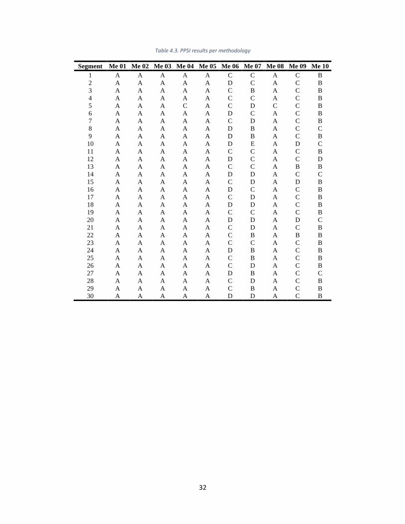
32

Table 4.3. PPSI results per methodology

Segment Me 01 Me 02 Me 03 Me 04 Me 05 Me 06 Me 07 Me 08 Me 09 Me 10

1 A A A A A C C A C B

2 A A A A A D C A C B

3 A A A A A C B A C B


5 A A A C A C D C C B


7 A A A A A C D A C B

8 A A A A A D B A C C

9 A A A A A D B A C B

10 A A A A A D E A D C


12 A A A A A D C A C D

13 A A A A A C C A B B

14 A A A A A D D A C C

15 A A A A A C D A D B



18 A A A A A D D A C B


20 A A A A A D D A D C


22 A A A A A C B A B B


24 A A A A A D B A C B



27 A A A A A D B A C C



30 A A A A A D D A C B

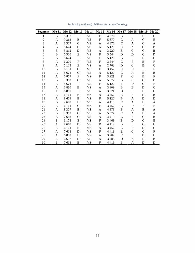
33

Table 4.3 (continued). PPSI results per methodology

Segment Me 11 Me 12 Me 13 Me 14 Me 15 Me 16 Me 17 Me 18 Me 19 Me 20

1 B 8.307 F VS F 4.876 B B B D

2 A 9.363 B VS F 5.577 C A C E

3 A 8.307 C VS A 4.876 C A C A

4 B 8.674 D VS A 5.120 C A C B

5 B 5.812 D VS A 3.220 B C C B

6 B 6.300 E VS F 3.544 D D C D

7 B 8.674 E VS C 5.120 B B B D

8 A 6.300 F VS F 3.544 C F B F

9 A 5.122 E VS A 2.763 D C B C

10 B 6.161 C MS F 3.452 C D E F

11 A 8.674 C VS A 5.120 C A B B

12 A 6.867 F VS F 3.921 F C B F

13 B 9.363 C VS A 5.577 B C C D

14 A 8.674 F VS F 5.120 F D C F

15 A 6.850 B VS A 3.909 B B D C

16 A 6.867 E VS A 3.921 D B B C

17 A 6.161 B MS A 3.452 B B D B

18 A 8.674 B VS F 5.120 B A D D

19 B 7.618 B VS A 4.419 C A B A

20 B 6.161 C MS F 3.452 C D E F

21 A 8.307 B VS A 4.876 B A B A

22 B 9.363 C VS A 5.577 C A B A

23 B 7.618 C VS A 4.419 C B C B

24 B 6.178 E VS F 3.463 B D C E

25 A 7.618 D VS D 4.419 B B C C

26 A 6.161 B MS A 3.452 C B D C

27 A 7.618 D VS F 4.419 E C C F

28 A 6.850 B VS A 3.909 C B D C

29 A 6.667 D VS A 3.788 D A B B

30 B 7.618 B VS F 4.419 B A D D

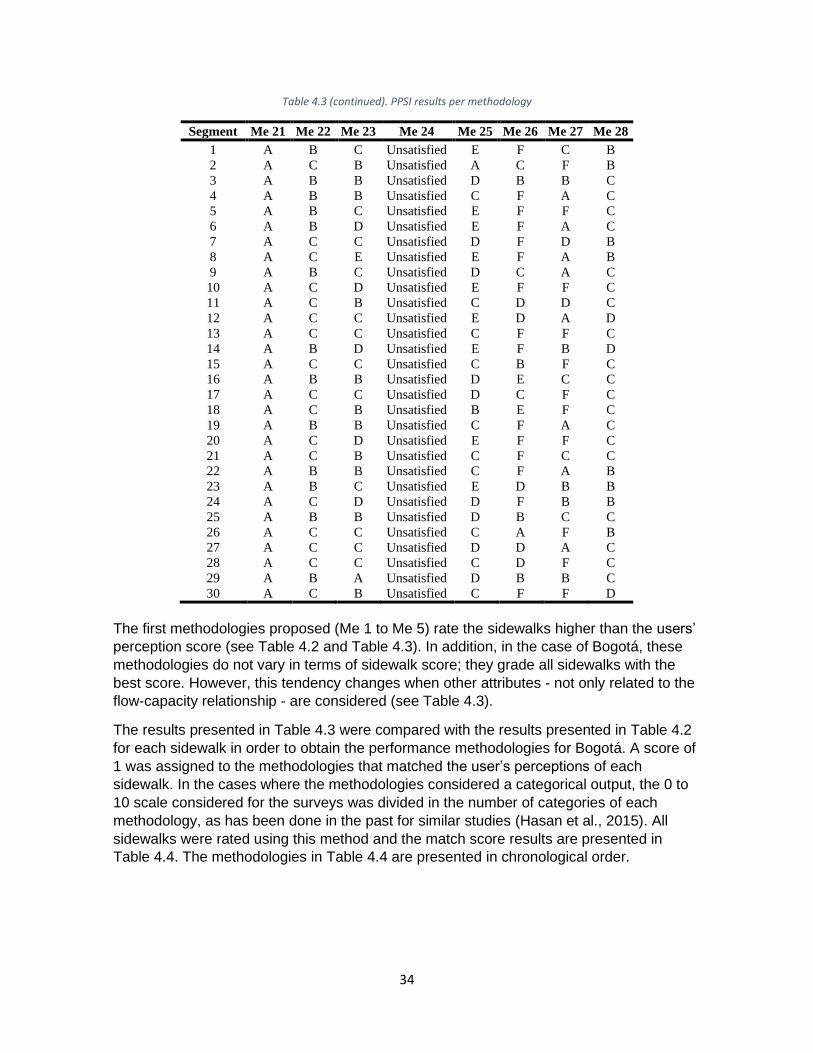
34

Table 4.3 (continued). PPSI results per methodology

Segment Me 21 Me 22 Me 23 Me 24 Me 25 Me 26 Me 27 Me 28

1 A B C Unsatisfied E F C B

2 A C B Unsatisfied A C F B

3 A B B Unsatisfied D B B C

4 A B B Unsatisfied C F A C

5 A B C Unsatisfied E F F C

6 A B D Unsatisfied E F A C

7 A C C Unsatisfied D F D B

8 A C E Unsatisfied E F A B

9 A B C Unsatisfied D C A C

10 A C D Unsatisfied E F F C

11 A C B Unsatisfied C D D C

12 A C C Unsatisfied E D A D

13 A C C Unsatisfied C F F C

14 A B D Unsatisfied E F B D

15 A C C Unsatisfied C B F C

16 A B B Unsatisfied D E C C

17 A C C Unsatisfied D C F C

18 A C B Unsatisfied B E F C

19 A B B Unsatisfied C F A C

20 A C D Unsatisfied E F F C

21 A C B Unsatisfied C F C C

22 A B B Unsatisfied C F A B

23 A B C Unsatisfied E D B B

24 A C D Unsatisfied D F B B

25 A B B Unsatisfied D B C C

26 A C C Unsatisfied C A F B

27 A C C Unsatisfied D D A C

28 A C C Unsatisfied C D F C

29 A B A Unsatisfied D B B C

30 A C B Unsatisfied C F F D

The first methodologies proposed (Me 1 to Me 5) rate the sidewalks higher than the users’

perception score (see Table 4.2 and Table 4.3). In addition, in the case of Bogotá, these

methodologies do not vary in terms of sidewalk score; they grade all sidewalks with the

best score. However, this tendency changes when other attributes - not only related to the

flow-capacity relationship - are considered (see Table 4.3).

The results presented in Table 4.3 were compared with the results presented in Table 4.2

for each sidewalk in order to obtain the performance methodologies for Bogotá. A score of

1 was assigned to the methodologies that matched the user’s perceptions of each

sidewalk. In the cases where the methodologies considered a categorical output, the 0 to

10 scale considered for the surveys was divided in the number of categories of each

methodology, as has been done in the past for similar studies (Hasan et al., 2015). All

sidewalks were rated using this method and the match score results are presented in

Table 4.4. The methodologies in Table 4.4 are presented in chronological order.

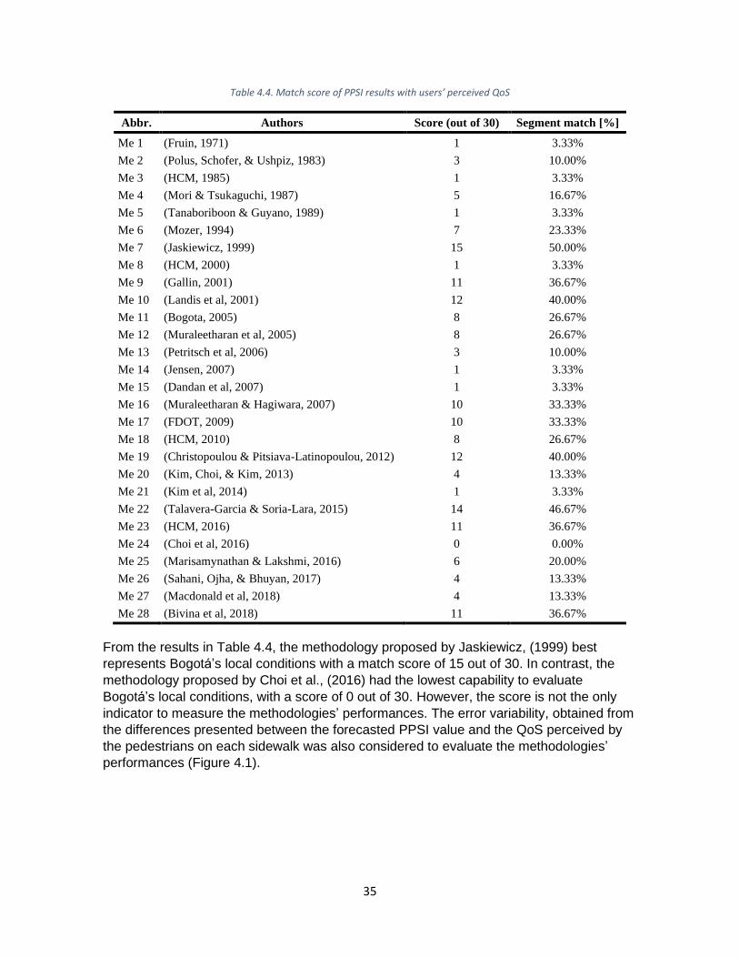
35

Table 4.4. Match score of PPSI results with users’ perceived QoS

Abbr. Authors Score (out of 30) Segment match [%]

Me 1 (Fruin, 1971) 1 3.33%

Me 2 (Polus, Schofer, & Ushpiz, 1983) 3 10.00%

Me 3 (HCM, 1985) 1 3.33%

Me 4 (Mori & Tsukaguchi, 1987) 5 16.67%

Me 5 (Tanaboriboon & Guyano, 1989) 1 3.33%

Me 6 (Mozer, 1994) 7 23.33%

Me 7 (Jaskiewicz, 1999) 15 50.00%

Me 8 (HCM, 2000) 1 3.33%

Me 9 (Gallin, 2001) 11 36.67%

Me 10 (Landis et al, 2001) 12 40.00%

Me 11 (Bogota, 2005) 8 26.67%

Me 12 (Muraleetharan et al, 2005) 8 26.67%

Me 13 (Petritsch et al, 2006) 3 10.00%

Me 14 (Jensen, 2007) 1 3.33%

Me 15 (Dandan et al, 2007) 1 3.33%

Me 16 (Muraleetharan & Hagiwara, 2007) 10 33.33%

Me 17 (FDOT, 2009) 10 33.33%

Me 18 (HCM, 2010) 8 26.67%

Me 19 (Christopoulou & Pitsiava-Latinopoulou, 2012) 12 40.00%

Me 20 (Kim, Choi, & Kim, 2013) 4 13.33%

Me 21 (Kim et al, 2014) 1 3.33%

Me 22 (Talavera-Garcia & Soria-Lara, 2015) 14 46.67%

Me 23 (HCM, 2016) 11 36.67%

Me 24 (Choi et al, 2016) 0 0.00%

Me 25 (Marisamynathan & Lakshmi, 2016) 6 20.00%

Me 26 (Sahani, Ojha, & Bhuyan, 2017) 4 13.33%

Me 27 (Macdonald et al, 2018) 4 13.33%

Me 28 (Bivina et al, 2018) 11 36.67%

From the results in Table 4.4, the methodology proposed by Jaskiewicz, (1999) best

represents Bogotá’s local conditions with a match score of 15 out of 30. In contrast, the

methodology proposed by Choi et al., (2016) had the lowest capability to evaluate

Bogotá’s local conditions, with a score of 0 out of 30. However, the score is not the only

indicator to measure the methodologies’ performances. The error variability, obtained from

the differences presented between the forecasted PPSI value and the QoS perceived by

the pedestrians on each sidewalk was also considered to evaluate the methodologies’

performances (Figure 4.1).

36

Figure 4.1. Methodologies’ errors boxplot

Concerning these error measure, most methodologies proposed in the 20th century predict

the PPSI to have a higher value than the QoS of the sidewalks. On the other hand,

methodologies proposed after 2016 predict the PPSI more conservatively. However, the

methodologies proposed between the years 2000 and 2016 perform better in terms of

error variability, with variations around an error of 0%. Of these, the methods proposed by

the State of Florida Department of Transportation (2009) and by the Transportation

Research Board (2010, 2016), perform better in terms of error variability for Bogotá (with a

median of 0% and variability around this median).

However, the previously mentioned methodologies use different inputs (flow-capacity

relation, objective attributes, and expert judgement) to calculate their PPSI. For this

reason, the performance results for the methodologies that consider the previously-

mentioned inputs, one by one, will be presented later. Table 4.5 shows the results for

different inputs in terms of mean and maximum performance rendered by the methods in

each group. The mean performance was calculated by averaging the match score for the

different methodologies considering each group of inputs. In addition, complete

performance results for each group of inputs can be seen in Figure 4.2, Figure 4.4, and

Figure 4.6.

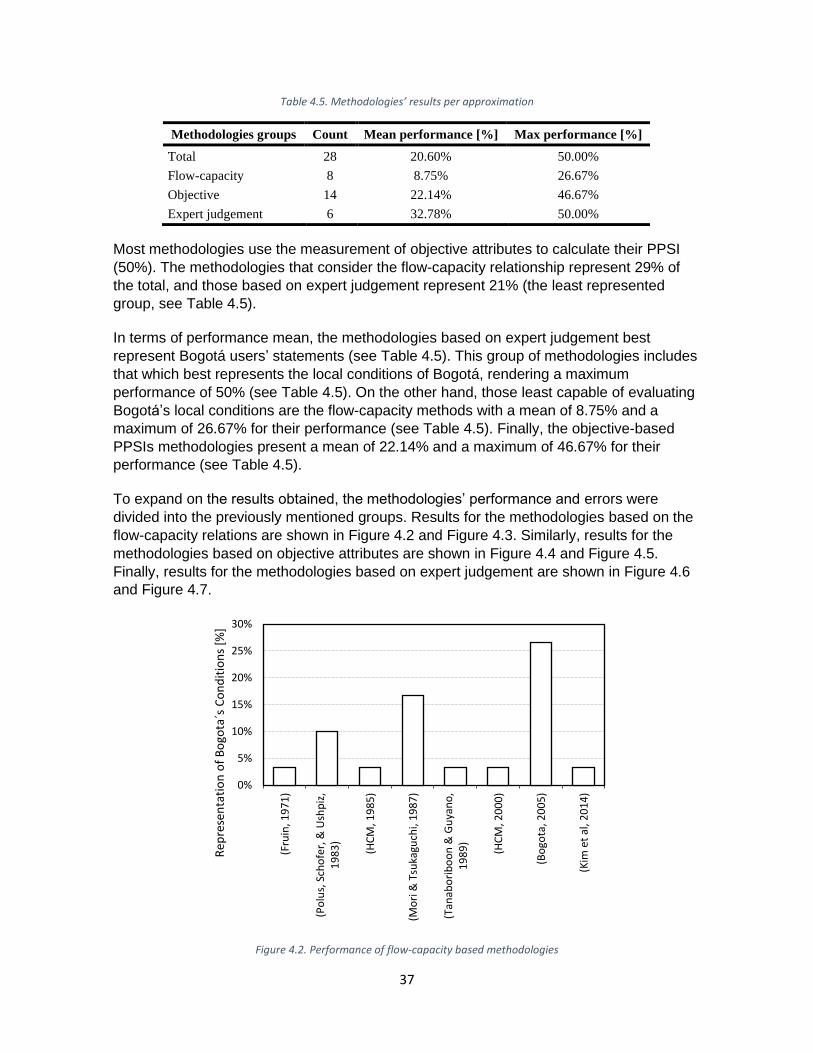
37

Table 4.5. Methodologies’ results per approximation

Most methodologies use the measurement of objective attributes to calculate their PPSI

(50%). The methodologies that consider the flow-capacity relationship represent 29% of

the total, and those based on expert judgement represent 21% (the least represented

group, see Table 4.5).

In terms of performance mean, the methodologies based on expert judgement best

represent Bogotá users’ statements (see Table 4.5). This group of methodologies includes

that which best represents the local conditions of Bogotá, rendering a maximum

performance of 50% (see Table 4.5). On the other hand, those least capable of evaluating

Bogotá’s local conditions are the flow-capacity methods with a mean of 8.75% and a

maximum of 26.67% for their performance (see Table 4.5). Finally, the objective-based

PPSIs methodologies present a mean of 22.14% and a maximum of 46.67% for their

performance (see Table 4.5).

To expand on the results obtained, the methodologies’ performance and errors were

divided into the previously mentioned groups. Results for the methodologies based on the

flow-capacity relations are shown in Figure 4.2 and Figure 4.3. Similarly, results for the

methodologies based on objective attributes are shown in Figure 4.4 and Figure 4.5.

Finally, results for the methodologies based on expert judgement are shown in Figure 4.6

and Figure 4.7.

Figure 4.2. Performance of flow-capacity based methodologies

0%

5%

10%

15%

20%

25%

30%

(Fru

in, 1

97

1)

(Po

lus,

Sch

ofe

r, &

Ush

piz

,1

98

3)

(HC

M, 1

98

5)

(Mo

ri &

Tsu

kagu

chi,

19

87

)

(Tan

abo

rib

oo

n &

Gu

yan

o,

19

89

)

(HC

M, 2

00

0)

(Bo

gota

, 20

05

)

(Kim

et

al, 2

01

4)

Rep

rese

nta

tio

n o

f B

ogo

ta´s

Co

nd

itio

ns

[%]

Methodologies groups Count Mean performance [%] Max performance [%]

Total 28 20.60% 50.00%

Flow-capacity 8 8.75% 26.67%

Objective 14 22.14% 46.67%

Expert judgement 6 32.78% 50.00%

38

In this group, the first PPSI method proposed is that developed by Fruin (1971), with a

performance below 5% (see Figure 4.2 and Table 4.4). Methodologies that consider the

flow-capacity relationship were the most commonly proposed methodologies for the

calculation of PPSI before the year 2000. Their performance did not improve because they

evolved, but because the PPSI’s possible results groups were reduced (see Appendix B –

Methodological review). However, it was found that the methodology proposed by Alcaldia

Mayor de Bogota D.C. (2005), which is a calibrated version for Bogotá of that proposed by

the Transportation Research Board (2000), has a performance of 26.67% (see Table 4.4),

which is the best one for this group of methodologies (see Figure 4.2).

Figure 4.3. Flow-capacity relation methodologies errors boxplot

Concerning errors, the proposed methodologies using a flow-capacity relationship, predict

the PPSI to be higher than the SQoS of the sidewalks. Similarly, there are no variations

between the errors obtained from almost all methodologies in this category. However,

there are two that are different. The methodology proposed by Mōri & Tsukaguchi (1987)

does not present much variation when it is applied to different sidewalks, with a positively

located interquartile range of error variability with value 0. On the other hand, the

methodology proposed by Alcaldia Mayor de Bogota D.C. (2005), has the largest

interquartile range in comparison with the other methods, reaching an error value of 0 for

the first quartile (see Figure 4.3).

39

Figure 4.4. Performance of objective attributes-based methodologies

The first methodology to consider objective attributes was proposed by Mozer (1994), with

a performance of 23.33% for Bogotá (see Figure 4.4 and Table 4.4). The next

methodology for this group was proposed by B. Landis et al. (2001) and has a

performance of 40%, representing an improvement in comparison with the previous ones

(see Figure 4.4 and Table 4.4). However, this improvement was not constant and the

performance of the four methodologies that followed — Dandan et al. (2007), Jensen

(2007), Muraleetharan et al. (2005), and Petritsch et al. (2006) — decreased when applied

to the case of Bogotá, reaching values of 3.33% (see Figure 4.4 and Table 4.4). This

tendency was repeated in the case of the four following methodologies (S. Kim et al.,

2013; Muraleetharan & Hagiwara, 2007; State of Florida Department of Transportation,

2009; Transportation Research Board, 2010), with an initial performance of 33.33% for

Muraleetharan & Hagiwara (2007) and a decrease in performance reaching values of

13.33% (see Figure 4.4 and Table 4.4). After this last stage, another methodology was

proposed by Talavera-Garcia & Soria-Lara (2015), which had a performance of 46.67%,

that is, the best performance rendered by the methodologies based on objective attributes.

However, subsequent methodologies did not improve in performance, but conversely,

decreased in performance, reaching values of 0%. In general, the improvement of the

performance for these methodologies varies over the years from 0% (Choi et al., 2016) to

46.67% (Talavera-Garcia & Soria-Lara, 2015).

0%

5%

10%

15%

20%

25%

30%

35%

40%

45%

50%

(Mo

zer,

19

94

)

(Lan

dis

et

al, 2

00

1)

(Mu

rale

eth

aran

et

al, 2

00

5)

(Pet

rits

ch e

t al

, 20

06

)

(Jen

sen

, 20

07

)

(Dan

dan

et

al, 2

00

7)

(Mu

rale

eth

aran

& H

agiw

ara,

20

07

)

(FD

OT,

20

09

)

(HC

M, 2

01

0)

(Kim

, Ch

oi,

& K

im, 2

01

3)

(Tal

ave

ra-G

arci

a &

So

ria-

Lara

, 20

15

)

(HC

M, 2

01

6)

(Ch

oi e

t al

, 20

16

)

(Sah

ani,

Ojh

a, &

Bh

uya

n, 2

01

7)

Rep

rese

nta

tio

n o

f B

ogo

ta´s

Co

nd

itio

ns

[%]

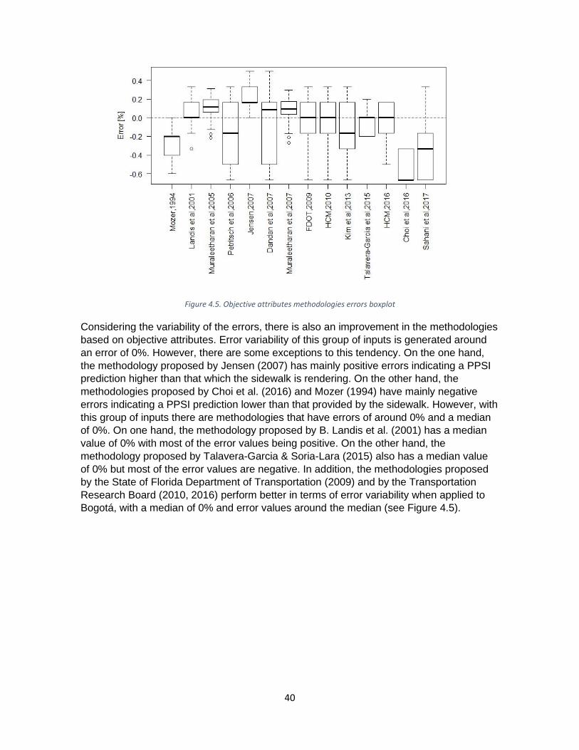
40

Figure 4.5. Objective attributes methodologies errors boxplot

Considering the variability of the errors, there is also an improvement in the methodologies

based on objective attributes. Error variability of this group of inputs is generated around

an error of 0%. However, there are some exceptions to this tendency. On the one hand,

the methodology proposed by Jensen (2007) has mainly positive errors indicating a PPSI

prediction higher than that which the sidewalk is rendering. On the other hand, the

methodologies proposed by Choi et al. (2016) and Mozer (1994) have mainly negative

errors indicating a PPSI prediction lower than that provided by the sidewalk. However, with

this group of inputs there are methodologies that have errors of around 0% and a median

of 0%. On one hand, the methodology proposed by B. Landis et al. (2001) has a median

value of 0% with most of the error values being positive. On the other hand, the

methodology proposed by Talavera-Garcia & Soria-Lara (2015) also has a median value

of 0% but most of the error values are negative. In addition, the methodologies proposed

by the State of Florida Department of Transportation (2009) and by the Transportation

Research Board (2010, 2016) perform better in terms of error variability when applied to

Bogotá, with a median of 0% and error values around the median (see Figure 4.5).

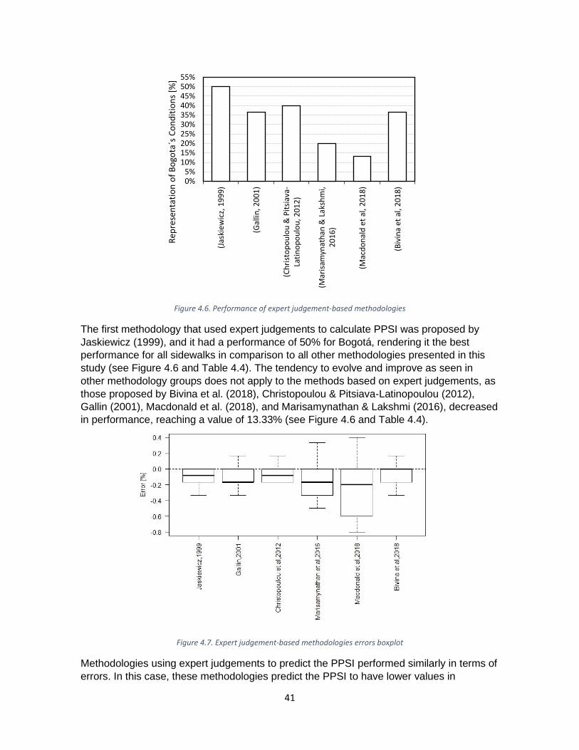
41

Figure 4.6. Performance of expert judgement-based methodologies

The first methodology that used expert judgements to calculate PPSI was proposed by

Jaskiewicz (1999), and it had a performance of 50% for Bogotá, rendering it the best

performance for all sidewalks in comparison to all other methodologies presented in this

study (see Figure 4.6 and Table 4.4). The tendency to evolve and improve as seen in

other methodology groups does not apply to the methods based on expert judgements, as

those proposed by Bivina et al. (2018), Christopoulou & Pitsiava-Latinopoulou (2012),

Gallin (2001), Macdonald et al. (2018), and Marisamynathan & Lakshmi (2016), decreased

in performance, reaching a value of 13.33% (see Figure 4.6 and Table 4.4).

Figure 4.7. Expert judgement-based methodologies errors boxplot

Methodologies using expert judgements to predict the PPSI performed similarly in terms of

errors. In this case, these methodologies predict the PPSI to have lower values in

0%5%

10%15%20%25%30%35%40%45%50%55%

(Jas

kie

wic

z, 1

99

9)

(Gal

lin, 2

00

1)

(Ch

rist

op

ou

lou

& P

itsi

ava-

Lati

no

po

ulo

u, 2

01

2)

(Mar

isam

ynat

han

& L

aksh

mi,

20

16

)

(Mac

do

nal

d e

t al

, 20

18

)

(Biv

ina

et a

l, 2

01

8)

Rep

rese

nta

tio

n o

f B

ogo

ta´s

Co

nd

itio

ns

[%]

42

comparison to the SQoS rendered by the sidewalks. However, the methodology proposed

by Bivina et al. (2018) has a median and third quartile equal to 0%, and is one of the

methodologies of this group with a lower error variability. Similarly, the methodologies

proposed by Christopoulou & Pitsiava-Latinopoulou (2012) and Jaskiewicz (1999) have

the lowest error variability not only for the expert judgement-based methodologies, but also

for all the methodologies presented in this study (see Figure 4.7).

The methodologies based on flow-capacity relation were the first, historically, proposed to

calculate PPSI, but are clearly not the best in terms of performance. Those based on

objective attributes have results with an error variability of around 0%, but with higher

variability in comparison to the expert judgement-based methodologies. In addition, the

expert judgement-based methodologies have the best mean and total performance.

Similarly, the expert judgement-based methodologies have the lowest error variation, in

spite of the small number of studies of this type found in the literature (see Table 4.5).

43

5. The influence of perceptions on the

QoS By uncovering the effects of perceptions on the perceived QoS, the previous results that

found that methodologies that calculate PPSI based on expert perceptions perform better

than others, can be taken advantage of. These effects will be uncovered by analyzing the

individual and joint effects of different groups of attributes (environmental,

sociodemographic, physical, and perceptual) on the perceived QoS. First, models will be

generated by considering the groups individually as independent variables. Then, the

groups in pairs and groups of threes and fours will be treated as independent variables. In

addition, a cognitive map describing how pedestrians perceive the QoS from their

perceptions of different sidewalk attributes will be developed.

The first step is to distinguish the overall contribution of the four different groups of

attributes from the overall QoS explanation (see Table 3.10). To start, a regression

analysis was done considering QoS to be the dependent variable, without combining the

different groups of attributes. From this regression, the coefficient of determination (R2)

was used to quantify how much of the total variance for the dependent variable was

explained by the different groups of attributes independent of each other.

We found that a model using only the environmental attributes explained the total variance

of the dependent variable least (R2 = 0.010). In addition, a model using sociodemographic

attributes only also explains little of the total variance (R2 = 0.026). Similarly, a model using

only physical attributes as independent variables explains much more of the total variance

in the dependent variable (R2 = 0.229). Finally, a model using only perception attributes

explains best the total variance of the perceived QoS (R2 = 0.574, see Figure 5.1 and

Table 5.1).

Figure 5.1. Proportion of the total variance explained by individual group regressions

0.0 0.1 0.2 0.3 0.4 0.5 0.6

M1 - E

M2 - S

M3 - Ph

M4 - Pe

R2

Environment (E)

Sociodemographic (S)

Physic (Ph)

Perception (Pe)

44

Table 5.1. Individual contribution to the overall R2

Model Environment (E) Sociodemographic (S) Physic (Ph) Perceptual (Pe)

M1 - E 0.009

M2 - S 0.026

M3 - Ph 0.229

M4 - Pe 0.574

The same analysis was carried out again, but this time, the different attribute groups were

considered as independent variables in pairs. This analysis was carried out twice for each

pair, and each time the order in which a group was included in the model was changed, to

quantify the upper and lower bounds of the contribution of each group of attributes. The

models that contained perception attributes explained more of the total variance of the

perceived QoS. On the other hand, the models containing environmental and

sociodemographic attributes explained the total variance of the dependent variable least

(see Figure 5.2).

Figure 5.2. Proportion of the total variance explained by group regressions in pairs

A model using physical and perception attributes explained the total variance of the

perceived QoS most (R2 = 0.597). However, there is a difference in how much each group

of variables contributes to the R2 depending on the order that this group is entered into the

model (see Table 5.3). When the environmental attributes are considered as an

independent variable, the lowest contribution of this group to the R2 is 0.002 and the

greatest is 0.010. Considering the sociodemographic attributes as the independent

variable, the lowest contribution of this group to the R2 is 0.011 and the greatest is 0.026.

The physical attributes as independent variable contribute 0.022 to the R2 at the lowest

and 0.229 at the greatest, values that overlap with the contribution of the R2 generated by

the sociodemographic attributes. Finally, the perception attributes as independent

variables contribute 0.372 to the R2 at the lowest and 0.578 at the greatest (see Table 5.2).

0.0 0.1 0.2 0.3 0.4 0.5 0.6 0.7

M5 - E/S

M5 - S/E

M6 - E/Ph

M6 - Ph/E

M7 - E/Pe

M7 - Pe/E

M8 - S/Ph

M8 - Ph/S

M9 - S/Pe

M9 - Pe/S

M10 - Ph/Pe

M10 - Pe/Ph

R2

Environment (E)


Physic (Ph)

Perception (Pe)

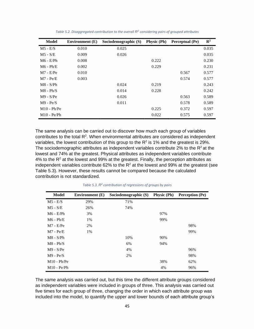
45

Table 5.2. Disaggregated contribution to the overall R2 considering pairs of grouped attributes

Model Environment (E) Sociodemographic (S) Physic (Ph) Perceptual (Pe) R2

M5 - E/S 0.010 0.025 0.035

M5 - S/E 0.009 0.026 0.035

M6 - E/Ph 0.008 0.222 0.230

M6 - Ph/E 0.002 0.229 0.231

M7 - E/Pe 0.010 0.567 0.577

M7 - Pe/E 0.003 0.574 0.577

M8 - S/Ph 0.024 0.219 0.243

M8 - Ph/S 0.014 0.228 0.242

M9 - S/Pe 0.026 0.563 0.589

M9 - Pe/S 0.011 0.578 0.589

M10 - Ph/Pe 0.225 0.372 0.597

M10 - Pe/Ph 0.022 0.575 0.597

The same analysis can be carried out to discover how much each group of variables

contributes to the total R2. When environmental attributes are considered as independent

variables, the lowest contribution of this group to the R2 is 1% and the greatest is 29%.

The sociodemographic attributes as independent variables contribute 2% to the R2 at the

lowest and 74% at the greatest. Physical attributes as independent variables contribute

4% to the R2 at the lowest and 99% at the greatest. Finally, the perception attributes as

independent variables contribute 62% to the R2 at the lowest and 99% at the greatest (see

Table 5.3). However, these results cannot be compared because the calculated

contribution is not standardized.

Table 5.3. R2 contribution of regressions of groups by pairs

Model Environment (E) Sociodemographic (S) Physic (Ph) Perception (Pe)

M5 - E/S 29% 71%

M5 - S/E 26% 74%

M6 - E/Ph 3% 97%

M6 - Ph/E 1% 99%

M7 - E/Pe 2% 98%

M7 - Pe/E 1% 99%

M8 - S/Ph 10% 90%

M8 - Ph/S 6% 94%

M9 - S/Pe 4% 96%

M9 - Pe/S 2% 98%

M10 - Ph/Pe 38% 62%

M10 - Pe/Ph 4% 96%

The same analysis was carried out, but this time the different attribute groups considered

as independent variables were included in groups of three. This analysis was carried out

five times for each group of three, changing the order in which each attribute group was

included into the model, to quantify the upper and lower bounds of each attribute group’s

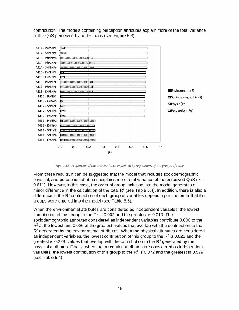
46

contribution. The models containing perception attributes explain more of the total variance

of the QoS perceived by pedestrians (see Figure 5.3).

Figure 5.3. Proportion of the total variance explained by regressions of the groups of three

From these results, it can be suggested that the model that includes sociodemographic,

physical, and perception attributes explains more total variance of the perceived QoS (r2 =

0.611). However, in this case, the order of group inclusion into the model generates a

minor difference in the calculation of the total R2 (see Table 5.4). In addition, there is also a

difference in the R2 contribution of each group of variables depending on the order that the

groups were entered into the model (see Table 5.5).

When the environmental attributes are considered as independent variables, the lowest

contribution of this group to the R2 is 0.002 and the greatest is 0.010. The

sociodemographic attributes considered as independent variables contribute 0.006 to the

R2 at the lowest and 0.026 at the greatest, values that overlap with the contribution to the

R2 generated by the environmental attributes. When the physical attributes are considered

as independent variables, the lowest contribution of this group to the R2 is 0.021 and the

greatest is 0.228, values that overlap with the contribution to the R2 generated by the

physical attributes. Finally, when the perception attributes are considered as independent

variables, the lowest contribution of this group to the R2 is 0.372 and the greatest is 0.579

(see Table 5.4).

0.0 0.1 0.2 0.3 0.4 0.5 0.6 0.7

M11 - E/S/Ph

M11 - S/E/Ph

M11 - S/Ph/E

M11 - E/Ph/S

M11 - Ph/E/S

M12 - E/S/Pe

M12 - S/E/Pe

M12 - S/Pe/E

M12 - E/Pe/S

M12 - Pe/E/S

M13 - E/Ph/Pe

M13 - Ph/E/Pe

M13 - Ph/Pe/E

M13 - E/Pe/Ph

M13 - Pe/E/Ph

M14 - S/Ph/Pe

M14 - Ph/S/Pe

M14 - Ph/Pe/S

M14 - S/Pe/Ph

M14 - Pe/S/Ph

R2

Environment (E)


Physic (Ph)

Perception (Pe)

47

Table 5.4. Disaggregated contribution to the overall R2 considering attribute groups in threes

Model Environment (E) Sociodemographic (S) Physic (Ph) Perception (Pe) R2

M11 - E/S/Ph 0.009 0.023 0.213 0.245

M11 - S/E/Ph 0.009 0.024 0.213 0.246

M11 - S/Ph/E 0.003 0.024 0.219 0.246

M11 - E/Ph/S 0.009 0.014 0.221 0.244

M11 - Ph/E/S 0.003 0.014 0.228 0.245

M12 - E/S/Pe 0.010 0.026 0.557 0.593

M12 - S/E/Pe 0.010 0.026 0.557 0.593

M12 - S/Pe/E 0.004 0.026 0.563 0.593

M12 - E/Pe/S 0.010 0.011 0.572 0.593

M12 - Pe/E/S 0.004 0.011 0.578 0.593

M13 - E/Ph/Pe 0.009 0.218 0.372 0.599

M13 - Ph/E/Pe 0.002 0.225 0.372 0.599

M13 - Ph/Pe/E 0.002 0.225 0.372 0.599

M13 - E/Pe/Ph 0.009 0.022 0.569 0.600

M13 - Pe/E/Ph 0.003 0.022 0.575 0.600

M14 - S/Ph/Pe 0.024 0.214 0.372 0.610

M14 - Ph/S/Pe 0.014 0.225 0.372 0.611

M14 - Ph/Pe/S 0.006 0.225 0.379 0.610

M14 - S/Pe/Ph 0.024 0.021 0.565 0.610

M14 - Pe/S/Ph 0.010 0.021 0.579 0.610

When the environmental attributes are considered as independent variables, the lowest

contribution of this group to the R2 is almost 0% and the greatest is 4%. In the case where

the sociodemographic attributes are considered as independent variables, the lowest

contribution of this group to the R2 is 1% and the greatest is 10%. In the case where the

physical attributes are considered as independent variables, the lowest contribution of this

group to the R2 is 3% and the greatest is 93%. Finally, in the case of the perception

attributes considered as independent variables, the lowest contribution of this group to the

R2 is 61% and the greatest is 97% (see Table 5.4). In this case the results presented

cannot be compared because the calculated contribution is not standardized.

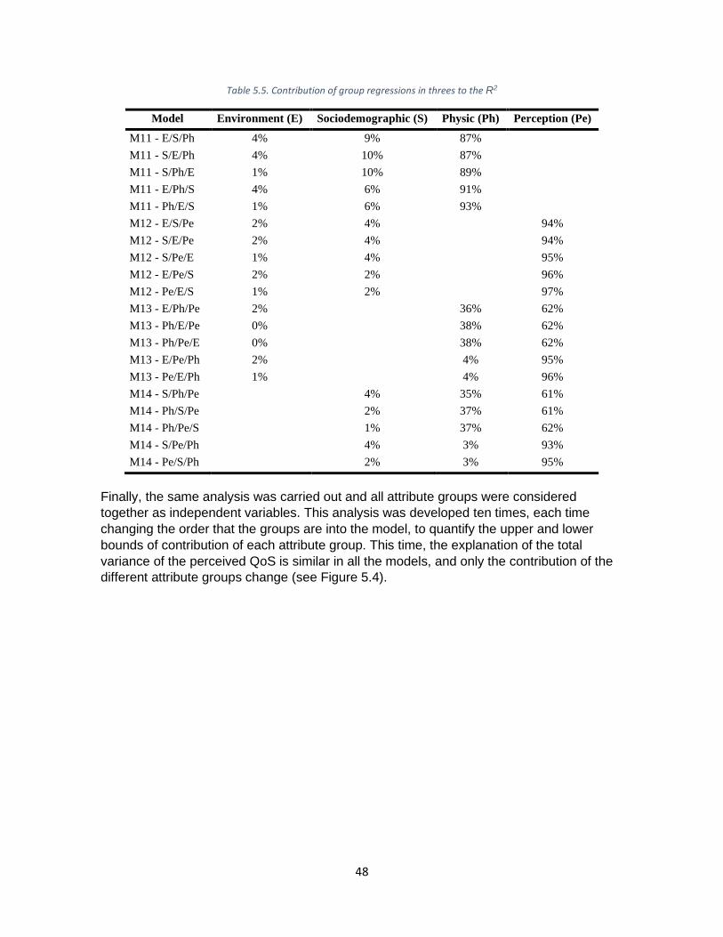
48

Table 5.5. Contribution of group regressions in threes to the R2


M11 - E/S/Ph 4% 9% 87%

M11 - S/E/Ph 4% 10% 87%

M11 - S/Ph/E 1% 10% 89%

M11 - E/Ph/S 4% 6% 91%

M11 - Ph/E/S 1% 6% 93%

M12 - E/S/Pe 2% 4% 94%

M12 - S/E/Pe 2% 4% 94%

M12 - S/Pe/E 1% 4% 95%

M12 - E/Pe/S 2% 2% 96%

M12 - Pe/E/S 1% 2% 97%

M13 - E/Ph/Pe 2% 36% 62%

M13 - Ph/E/Pe 0% 38% 62%

M13 - Ph/Pe/E 0% 38% 62%

M13 - E/Pe/Ph 2% 4% 95%

M13 - Pe/E/Ph 1% 4% 96%

M14 - S/Ph/Pe 4% 35% 61%

M14 - Ph/S/Pe 2% 37% 61%

M14 - Ph/Pe/S 1% 37% 62%

M14 - S/Pe/Ph 4% 3% 93%

M14 - Pe/S/Ph 2% 3% 95%

Finally, the same analysis was carried out and all attribute groups were considered

together as independent variables. This analysis was developed ten times, each time

changing the order that the groups are into the model, to quantify the upper and lower

bounds of contribution of each attribute group. This time, the explanation of the total

variance of the perceived QoS is similar in all the models, and only the contribution of the

different attribute groups change (see Figure 5.4).

49

Figure 5.4. Proportion of the total variance explained by regressions of total groups

The model that explains the most total variance of the perceived QoS does not depend on

the order of groups into the model, generating an R2 of 0.614 (see Table 5.6). When the

environmental attributes are considered as independent variables, the lowest contribution

of this group to the R2 is 0.003 and the greatest is 0.010. Where the sociodemographic

attributes are considered as independent variables, the lowest contribution of this group to

the R2 is 0.007 and the greatest is 0.024, values that overlap with the contribution to the R2

generated by the environmental attributes. Where the physical attributes are considered as

independent variables, the lowest contribution of this group to the R2 is 0.021 and the

greatest is 0.225, values that overlap with the contribution to the R2 generated by the

physical attributes. Finally, where the perception attributes are considered as independent

variables, the lowest contribution of this group to the R2 is 0.372 and the greatest is 0.579,

which does not overlap with any of the other figures obtained (see Table 5.6).

Table 5.6. Disaggregated contribution to the overall R2 considering all groups of attributes

Model Environment (E) Sociodemographic (S) Physic (Ph) Perception (Pe) R2

M15 - E/S/Ph/Pe 0.010 0.024 0.208 0.372 0.614

M15 - S/E/Ph/Pe 0.009 0.024 0.208 0.372 0.613

M15 - S/Ph/E/Pe 0.003 0.024 0.214 0.372 0.613

M15 - S/Ph/Pe/E 0.003 0.024 0.214 0.372 0.613

M15 - E/Ph/S/Pe 0.010 0.007 0.218 0.379 0.614

M15 - E/Ph/Pe/S 0.010 0.007 0.218 0.379 0.614

M15 - Ph/E/S/Pe 0.003 0.014 0.225 0.372 0.614

M15 - E/S/Pe/Ph 0.010 0.024 0.021 0.559 0.614

M15 - Pe/E/S/Ph 0.003 0.010 0.021 0.579 0.613

M15 - E/Pe/S/Ph 0.010 0.010 0.021 0.572 0.613

There is also a difference in the R2 contribution of each group of variables depending on

the order in which the groups are entered into the model when considering the contribution

0.0 0.1 0.2 0.3 0.4 0.5 0.6 0.7

M15 - E/S/Ph/Pe

M15 - S/E/Ph/Pe

M15 - S/Ph/E/Pe

M15 - S/Ph/Pe/E

M15 - E/Ph/S/Pe

M15 - E/Ph/Pe/S

M15 - Ph/E/S/Pe

M15 - E/S/Pe/Ph

M15 - Pe/E/S/Ph

M15 - E/Pe/S/Ph

R2

Environment (E)


Physic (Ph)

Perception (Pe)

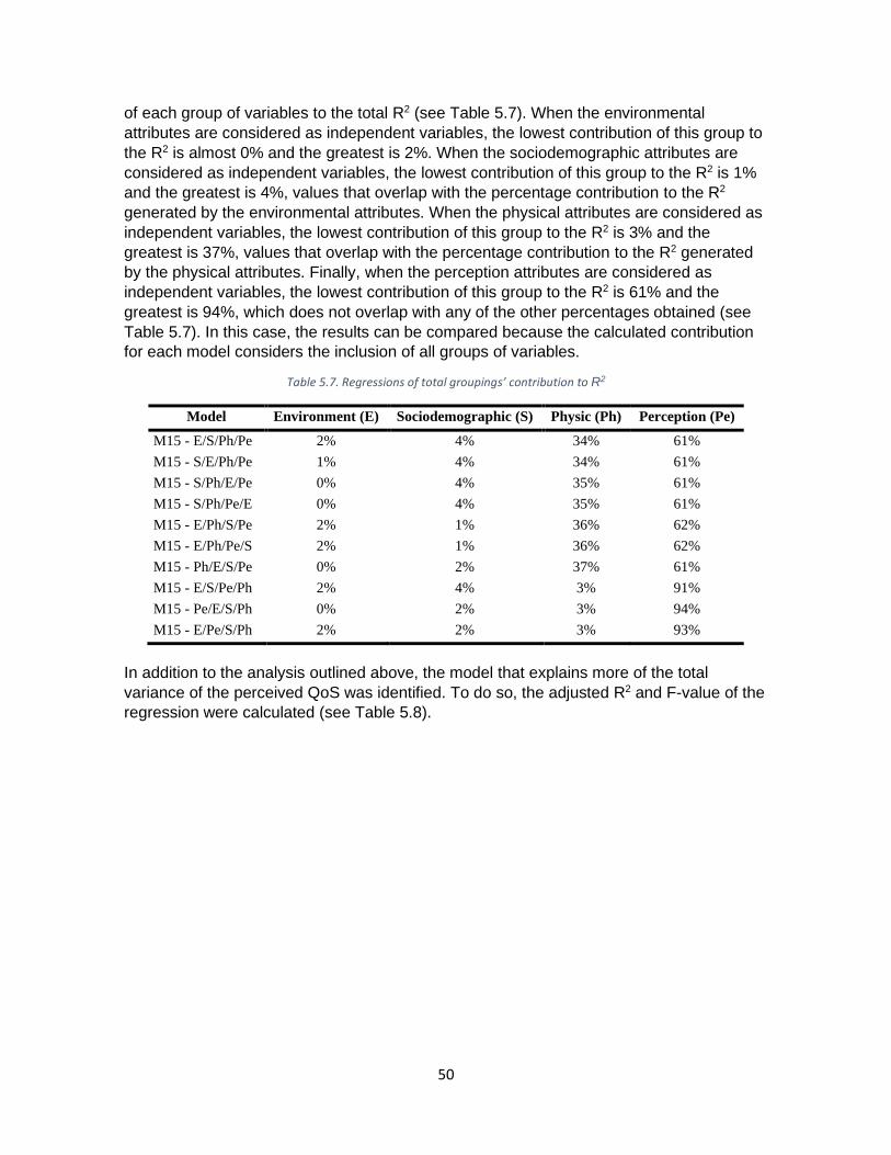
50

of each group of variables to the total R2 (see Table 5.7). When the environmental

attributes are considered as independent variables, the lowest contribution of this group to

the R2 is almost 0% and the greatest is 2%. When the sociodemographic attributes are

considered as independent variables, the lowest contribution of this group to the R2 is 1%

and the greatest is 4%, values that overlap with the percentage contribution to the R2

generated by the environmental attributes. When the physical attributes are considered as

independent variables, the lowest contribution of this group to the R2 is 3% and the

greatest is 37%, values that overlap with the percentage contribution to the R2 generated

by the physical attributes. Finally, when the perception attributes are considered as

independent variables, the lowest contribution of this group to the R2 is 61% and the

greatest is 94%, which does not overlap with any of the other percentages obtained (see

Table 5.7). In this case, the results can be compared because the calculated contribution

for each model considers the inclusion of all groups of variables.

Table 5.7. Regressions of total groupings’ contribution to R2


M15 - E/S/Ph/Pe 2% 4% 34% 61%

M15 - S/E/Ph/Pe 1% 4% 34% 61%

M15 - S/Ph/E/Pe 0% 4% 35% 61%

M15 - S/Ph/Pe/E 0% 4% 35% 61%

M15 - E/Ph/S/Pe 2% 1% 36% 62%

M15 - E/Ph/Pe/S 2% 1% 36% 62%

M15 - Ph/E/S/Pe 0% 2% 37% 61%

M15 - E/S/Pe/Ph 2% 4% 3% 91%

M15 - Pe/E/S/Ph 0% 2% 3% 94%

M15 - E/Pe/S/Ph 2% 2% 3% 93%

In addition to the analysis outlined above, the model that explains more of the total

variance of the perceived QoS was identified. To do so, the adjusted R2 and F-value of the

regression were calculated (see Table 5.8).

51

Table 5.8. Adjusted R2 and F-value for the models’ regressions

Model Adjusted R2 F-value (regression)

M1 0.005 2.341

M2 0.024 2.442

M3 0.190 5.945

M4 0.564 27.138

M5 0.027 2.351

M6 0.189 5.526

M7 0.565 25.236

M8 0.198 4.595

M9 0.564 19.024

M10 0.563 13.492

M11 0.197 4.359

M12 0.565 18.063

M13 0.564 13.040

M14 0.559 10.821

M15 0.560 10.507

Two models (M7 and M12) can be selected as having the best fit using the adjusted R2 as

the goodness of fit indicator. Both models use the perception and environmental attributes

as independent variables. Using the F-value of the regression as the indicator for choosing

the best model, one model (M4) appears to be the best. This model was developed using

the perception attributes as independent variables. There are three different options to

identify which attributes, used as independent variables, generate the best model in terms

of goodness of fit. Nonetheless, the three models all use the perception group as

independent variables to explain the perceived QoS variance. To identify the best model

considering both adjusted R2 and F-value, a MAUT analysis was carried out by weighting

each of the goodness of fit indicators. Through this analysis, a value between 0 and 1 was

obtained for each model; where this value is higher it is suggested that the model is better

in terms of goodness of fit. The results obtained for each model are presented in Table 5.9

and the comparison positions of different models are presented in Table 5.10.

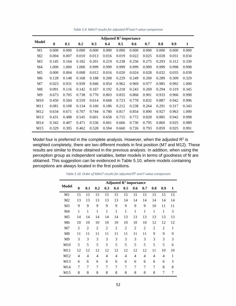
52

Table 5.9. MAUT results for adjusted R2and F-value comparison

Model Adjusted R2 importance

0 0.1 0.2 0.3 0.4 0.5 0.6 0.7 0.8 0.9 1

M1 0.000 0.000 0.000 0.000 0.000 0.000 0.000 0.000 0.000 0.000 0.000

M2 0.004 0.007 0.010 0.013 0.016 0.019 0.022 0.025 0.028 0.031 0.034

M3 0.145 0.164 0.182 0.201 0.219 0.238 0.256 0.275 0.293 0.312 0.330

M4 1.000 1.000 1.000 0.999 0.999 0.999 0.999 0.999 0.999 0.998 0.998

M5 0.000 0.004 0.008 0.012 0.016 0.020 0.024 0.028 0.032 0.035 0.039

M6 0.128 0.148 0.168 0.188 0.208 0.229 0.249 0.269 0.289 0.309 0.329

M7 0.923 0.931 0.939 0.946 0.954 0.962 0.969 0.977 0.985 0.992 1.000

M8 0.091 0.116 0.142 0.167 0.192 0.218 0.243 0.269 0.294 0.319 0.345

M9 0.673 0.705 0.738 0.770 0.803 0.835 0.868 0.901 0.933 0.966 0.998

M10 0.450 0.504 0.559 0.614 0.668 0.723 0.778 0.832 0.887 0.942 0.996

M11 0.081 0.108 0.134 0.160 0.186 0.212 0.238 0.264 0.291 0.317 0.343

M12 0.634 0.671 0.707 0.744 0.780 0.817 0.854 0.890 0.927 0.963 1.000

M13 0.431 0.488 0.545 0.601 0.658 0.715 0.772 0.828 0.885 0.942 0.998

M14 0.342 0.407 0.471 0.536 0.601 0.666 0.730 0.795 0.860 0.925 0.989

M15 0.329 0.395 0.462 0.528 0.594 0.660 0.726 0.793 0.859 0.925 0.991

Model four is preferred in the complete analysis. However, when the adjusted R2 is

weighted completely, there are two different models in first position (M7 and M12). These

results are similar to those obtained in the previous analysis. In addition, when using the

perception group as independent variables, better models in terms of goodness of fit are

obtained. This suggestion can be evidenced in Table 5.10, where models containing

perceptions are always located in the first positions.

Table 5.10. Order of MAUT results for adjusted R2 and F-value comparison

Model Adjusted R2 importance

0 0.1 0.2 0.3 0.4 0.5 0.6 0.7 0.8 0.9 1

M1 15 15 15 15 15 15 15 15 15 15 15

M2 13 13 13 13 13 14 14 14 14 14 14

M3 9 9 9 9 9 9 9 9 10 11 11

M4 1 1 1 1 1 1 1 1 1 1 3

M5 14 14 14 14 14 13 13 13 13 13 13

M6 10 10 10 10 10 10 10 10 12 12 12

M7 2 2 2 2 2 2 2 2 2 2 1

M8 11 11 11 11 11 11 11 11 9 9 9

M9 3 3 3 3 3 3 3 3 3 3 3

M10 5 5 5 5 5 5 5 5 5 5 6

M11 12 12 12 12 12 12 12 12 11 10 10

M12 4 4 4 4 4 4 4 4 4 4 1

M13 6 6 6 6 6 6 6 6 6 6 3

M14 7 7 7 7 7 7 7 7 7 8 8

M15 8 8 8 8 8 8 8 8 8 7 7

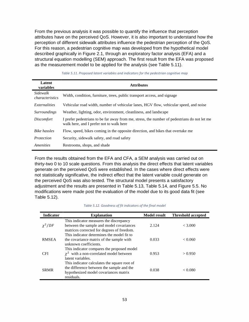
53

From the previous analysis it was possible to quantify the influence that perception

attributes have on the perceived QoS. However, it is also important to understand how the

perception of different sidewalk attributes influence the pedestrian perception of the QoS.

For this reason, a pedestrian cognitive map was developed from the hypothetical model

described graphically in Figure 2.1, through an exploratory factor analysis (EFA) and a

structural equation modelling (SEM) approach. The first result from the EFA was proposed

as the measurement model to be applied for the analysis (see Table 5.11).

Table 5.11. Proposed latent variables and indicators for the pedestrian cognitive map

Latent

variables Attributes

Sidewalk

characteristics Width, condition, furniture, trees, public transport access, and signage

Externalities Vehicular road width, number of vehicular lanes, HGV flow, vehicular speed, and noise

Surroundings Weather, lighting, odor, environment, cleanliness, and landscape

Discomfort I prefer pedestrians to be far away from me, stress, the number of pedestrians do not let me

walk here, and I prefer not to walk here

Bike hassles Flow, speed, bikes coming in the opposite direction, and bikes that overtake me

Protection Security, sidewalk safety, and road safety

Amenities Restrooms, shops, and shade

From the results obtained from the EFA and CFA, a SEM analysis was carried out on

thirty-two 0 to 10 scale questions. From this analysis the direct effects that latent variables

generate on the perceived QoS were established. In the cases where direct effects were

not statistically significative, the indirect effect that the latent variable could generate on

the perceived QoS was also tested. The structural model presents a satisfactory

adjustment and the results are presented in Table 5.13, Table 5.14, and Figure 5.5. No

modifications were made post the evaluation of the model due to its good data fit (see

Table 5.12).

Table 5.12. Goodness of fit indicators of the final model

Indicator Explanation Model result Threshold accepted

𝜒2 𝐷𝐹⁄

This indicator measures the discrepancy

between the sample and model covariances

matrices corrected for degrees of freedom.

2.124 < 3.000

RMSEA

This indicator determines the model fit to

the covariance matrix of the sample with

unknown coefficients.

0.033 < 0.060

CFI

This indicator compares the proposed model

𝜒2 with a non-correlated model between

latent variables.

0.953 > 0.950

SRMR

This indicator calculates the square root of

the difference between the sample and the

hypothesized model covariances matrix

residuals.

0.038 < 0.080

54

The measurement model was proposed in Table 5.11, and it was tested by obtaining

statistically significative results (see Table 5.13). From the measurement model, the

existence of seven latent variables were statistically proven from thirty-one attributes of

pedestrians’ perceptions when walking on urban sidewalks. The most robust latent

variables are the sidewalk characteristics and surroundings, with six indicators in each of

these. The externalities contain five indicators, and the discomfort and bike hassles are

composed of four indicators each. Finally, protection and amenities contain three

indicators each.

Table 5.13. Standardized parameters of measurement model

Attribute Latent variable 𝜶 𝝀 t-statistic

Service quality - 2.383 - 39.068

Width

Sidewalk

characteristics

1.771 0.708 35.702

Condition 1.550 0.731 33.871

Furniture 1.473 0.640 28.736

Trees 1.225 0.586 24.424

Public transit access 1.650 0.422 14.636

Signage 1.363 0.625 28.392

Road width

Externalities

1.016 0.619 21.854

Lanes 1.034 0.621 21.677

HGV flow 1.315 0.636 21.593

Vehicular speed 1.428 0.629 21.480

Noise 2.489 0.381 11.631

Weather

Surroundings

2.671 0.373 12.448

Lighting 3.451 0.418 14.042

Odor 1.971 0.665 25.665

Environment 2.568 0.778 41.976

Cleanliness 1.711 0.713 35.363

Landscape 2.184 0.679 31.912

Pedestrians far from me

Discomfort

1.137 0.462 15.880

Stress 1.033 0.750 35.082

Too many pedestrians 1.071 0.704 31.410

I prefer not to walk here 0.942 0.631 25.918

Bike flow

Bike hassles

2.289 0.753 41.244

Bike speed 3.737 0.851 53.889

Opposite direction flow 2.690 0.627 27.970

Same direction flow 2.868 0.647 29.798

Security

Protection

1.039 0.653 28.704

Sidewalk safety 1.325 0.824 42.785

Road safety 1.401 0.726 34.565

Restrooms

Amenities

1.530 0.433 10.305

Shops 2.887 0.589 12.451

Shade 3.148 0.471 10.947

Additionally, the structural model was tested by obtaining statistically significative results

(see Table 5.14 and Figure 5.5). From the structural model, it was statistically proven that

the QoS perception is directly explained by the perception of sidewalk characteristics and

surroundings. In addition, how the sidewalk characteristics is perceived, is affected by the

perception of surroundings, externalities, discomfort, and protection. Similarly, the

perception of surroundings is affected by how pedestrians perceive externalities,

discomfort, and protection. In turn, the perception of externalities affects the way

pedestrians perceive discomfort and protection. Similarly, the perception of discomfort

55

affects protection. Finally, the way pedestrians perceive bike hassles and amenities affect

the perception of externalities and protection. Indeed, the cognitive map in Figure 5 shows

a complex web of interactions among variables.

Table 5.14. SEM infrastructure QoS final model results

MODEL

𝜷 𝒂𝒏𝒅 𝝀

Sidewalk

characteristics Surrounding Externalities Discomfort Protection

Bike

hassles Amenities

Direct

Service

quality 0.689 0.149

(t-statistic) (29.040) (5.114)

Sidewalk

characteristics 0.176 -0.363 -0.088 0.185

(t-statistic) (4.229) (-7.621) (-1.952) (4.838)

Surrounding -0.196 -0.170 0.350

(t-statistic) (-3.940) (-3.690) (9.973)

Externalities 0.156 -0.304

(t-statistic) (3.890) (-6.068)

Discomfort 0.527

(t-statistic) (14.590)

Protection -0.186 -0.100 -0.117 0.088

(t-statistic) (-3.217) (-1.972) (-3.088) (1.707)

Indirect

Service

quality 0.121 -0.412 -0.128 0.222 -0.091 0.145

(t-statistic) (4.153) (-14.736) (-3.659) (8.375) (-4.839) (6.021)

Sidewalk

characteristics -0.155 -0.055 0.062 -0.110 0.179

(t-statistic) (-5.696) (-3.237) (3.868) (-4.784) (6.067)

Surrounding -0.173 -0.035 -0.099 0.143

(t-statistic) (-5.776) (-1.933) (-4.912) (5.433)

Externalities

(t-statistic)

Discomfort 0.083 -0.160

(t-statistic) (3.747) (-5.561)

Protection -0.053 -0.037 0.072

(t-statistic) (-1.972) (-3.126) (3.992)

Total

Service

quality 0.689 0.270 -0.412 -0.128 0.222 -0.091 0.145

(t-statistic) (29.040) (7.747) (-14.736) (-3.659) (8.375) (-4.839) (6.021)

Sidewalk

characteristics 0.176 -0.519 -0.142 0.247 -0.110 0.179

(t-statistic) (4.229) (-15.009) (-3.035) (7.009) (-4.784) (6.067)

Surrounding -0.369 -0.205 0.350 -0.099 0.143

(t-statistic) (-9.482) (-4.256) (9.973) (-4.912) (5.433)

Externalities 0.156 -0.304

(t-statistic) (3.890) (-6.068)

Discomfort 0.527 0.083 -0.160

(t-statistic) (14.590) (3.747) (5.561)

Protection -0.238 -0.100 -0.155 0.161

(t-statistic) (-5.224) (-1.972) (-4.119) (3.348)

56

Figure 5.5. SEM infrastructure QoS final model

Perceived QoS is directly affected by two latent variables: sidewalk characteristics and

surroundings; and indirectly affected by six latent variables: surrounding, externalities,

discomfort, protection, bike hassles, and amenities. In the case of direct effects, the

perception of QoS is directly and positively affected by the perception of sidewalk

characteristics (𝜆 = 0.689). Similarly, the perception of surroundings is directly and

positively related to the perceived QoS (𝜆 = 0.149). Additionally, when indirect effects are

considered, the perception of QoS is also positively affected by the perception of the

surroundings using the sidewalk characteristics as a mediator (𝑤 = 0.121). Similarly, the

perceived QoS is also affected in a positive and indirect way by how pedestrians perceive

their protection (𝑤 = 0.222) and amenities (𝑤 = 0.145), using as final mediators the

perception of surroundings and sidewalk characteristics. On the other hand, the perception

of externalities also indirectly affects the QoS perception, but in a negative way, with the

final mediation of the perception of surroundings and sidewalk characteristics (𝑤 =

−0.412). Similarly, the perceived QoS is also affected in a negative and indirect way by

how pedestrians perceive discomfort (𝑤 = −0.128) and bike hassles (𝑤 = −0.091), using

as final mediators the perceptions of surroundings and sidewalk characteristics.

57

6. Application of pedestrian

perceptions for QoS forecasting We considered the ordered probit model to be the best approach for forecasting the SQoS,

because it produced the best performance indicators when validated. However, applying

this model requires both objective (sidewalk and users attributes) and subjective

(pedestrian perceptions) information. On the other hand, of the models that only need user

and sidewalk objective attributes to explain the subjective attributes and to forecast SQoS,

the ordered probit MIMIC model would be the first choice. In both cases, the proposed

forecasting models represent Bogotá’s local context well in comparison with the previously

analyzed methodologies (see Figure 6.1). The forecasting models were based on the

complete description of the effects and roles that perceptions have on and in the

pedestrian QoS explanation.

Figure 6.1. Performance of proposed forecasting models vs existing methodologies

Initially, a linear model was proposed between the pedestrian perception of QoS and the

independent variables. This analysis was done using a forward approach and the final

model selection was based on the lower AIC estimator value. The obtained linear model is

presented in Table 6.1.

50.00%

26.67%

46.67%

96.67%

86.67%

0%

10%

20%

30%

40%

50%

60%

70%

80%

90%

100%

(Jaskiewicz, 1999) (Bogota, 2005) (Talavera-Garcia &Soria-Lara, 2015)

Ordered probit Ordered probitMIMIC

Rep

rese

nta

tio

n o

f B

ogo

ta´s

Co

nd

itio

ns

[%]

58

Table 6.1. Forecasting QoS linear model

Infrastructure service (QoS) forecasting by linear model

Adjusted R2 0.569

F-statistic 54.590

Estimate Std. Error t statistic p-value Sig

(Intercept) 0.896 0.381 2.353 0.019 *

Sidewalk surface condition1 0.216 0.032 6.830 0.000 ***

Building articulation1 0.243 0.031 7.918 0.000 ***

Sidewalk width1 0.156 0.030 5.189 0.000 ***

Horizontal marking1 0.091 0.026 3.533 0.000 ***

Road safety1 0.050 0.023 2.182 0.030 *

Sidewalk furniture1 0.067 0.029 2.292 0.022 *

Heavy vehicles1 -0.043 0.021 -2.077 0.038 *

Lighting1 0.073 0.032 2.284 0.023 *

Organized space1 0.050 0.024 2.116 0.035 *

Tree presence1 0.046 0.027 1.743 0.082 .

Facade distance [m] -0.019 0.007 -2.793 0.005 **

Trees [#] 0.019 0.012 1.597 0.111

Age [years] 0.011 0.005 2.227 0.026 *

Vehicular flow is close to me1 -0.035 0.021 -1.678 0.094 .

Bike infrastructure width [m] -0.130 0.081 -1.604 0.109

Significance codes: *** p < 0.001, ** p < 0.010, * p < 0.050, · p < 0.100

1. Pedestrian perception responses in situ from 0 to 10

The QoS forecasting linear model presents an adjusted R2 of 0.569 and has 15

independent variables. There are 11 perceptual variables and four objective variables. Out

of the perceptual variables, nine improve the QoS perceived by pedestrians, where the

perceived articulation of the different building facades and the perceived condition of the

sidewalk surface are the variables that most improve the perceived QoS. On the other

hand, the perceived heavy goods vehicle (HGV) flow and the perceived distance from the

vehicular flow are variables that decrease the pedestrian perception of the QoS. From the

objective variables, the analysis identified that the older the respondent and higher the

number of trees on the sidewalk, the higher was the perceived QoS. On the other hand,

the model also implied that the greater the distance from the sidewalk to the facade and

the bicycle infrastructure width, the lower the perceived QoS (see Table 6.1).

An ordered probit model was also proposed when a non-linear relationship between the

perceived QoS and the independent variables was considered. This analysis was carried

out using a forward approach and the final model selection was based on the lower AIC

estimator value. The obtained linear model is presented in Table 6.2.

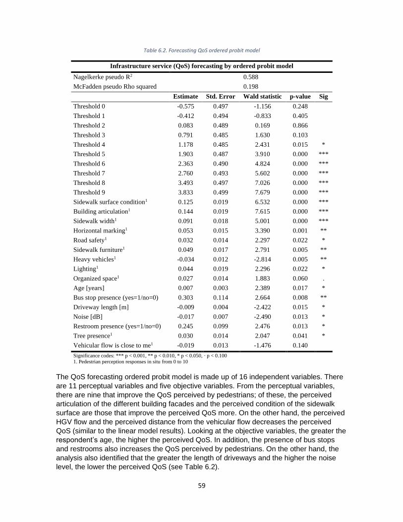
59

Table 6.2. Forecasting QoS ordered probit model

Infrastructure service (QoS) forecasting by ordered probit model

Nagelkerke pseudo R2 0.588

McFadden pseudo Rho squared 0.198

Estimate Std. Error Wald statistic p-value Sig

Threshold 0 -0.575 0.497 -1.156 0.248

Threshold 1 -0.412 0.494 -0.833 0.405

Threshold 2 0.083 0.489 0.169 0.866

Threshold 3 0.791 0.485 1.630 0.103

Threshold 4 1.178 0.485 2.431 0.015 *

Threshold 5 1.903 0.487 3.910 0.000 ***

Threshold 6 2.363 0.490 4.824 0.000 ***

Threshold 7 2.760 0.493 5.602 0.000 ***

Threshold 8 3.493 0.497 7.026 0.000 ***

Threshold 9 3.833 0.499 7.679 0.000 ***

Sidewalk surface condition1 0.125 0.019 6.532 0.000 ***

Building articulation1 0.144 0.019 7.615 0.000 ***

Sidewalk width1 0.091 0.018 5.001 0.000 ***

Horizontal marking1 0.053 0.015 3.390 0.001 **

Road safety1 0.032 0.014 2.297 0.022 *

Sidewalk furniture1 0.049 0.017 2.791 0.005 **

Heavy vehicles1 -0.034 0.012 -2.814 0.005 **

Lighting1 0.044 0.019 2.296 0.022 *

Organized space1 0.027 0.014 1.883 0.060 .

Age [years] 0.007 0.003 2.389 0.017 *

Bus stop presence (yes=1/no=0) 0.303 0.114 2.664 0.008 **

Driveway length [m] -0.009 0.004 -2.422 0.015 *

Noise [dB] -0.017 0.007 -2.490 0.013 *

Restroom presence (yes=1/no=0) 0.245 0.099 2.476 0.013 *

Tree presence1 0.030 0.014 2.047 0.041 *

Vehicular flow is close to me1 -0.019 0.013 -1.476 0.140

Significance codes: *** p < 0.001, ** p < 0.010, * p < 0.050, · p < 0.100 1. Pedestrian perception responses in situ from 0 to 10

The QoS forecasting ordered probit model is made up of 16 independent variables. There

are 11 perceptual variables and five objective variables. From the perceptual variables,

there are nine that improve the QoS perceived by pedestrians; of these, the perceived

articulation of the different building facades and the perceived condition of the sidewalk

surface are those that improve the perceived QoS more. On the other hand, the perceived

HGV flow and the perceived distance from the vehicular flow decreases the perceived

QoS (similar to the linear model results). Looking at the objective variables, the greater the

respondent’s age, the higher the perceived QoS. In addition, the presence of bus stops

and restrooms also increases the QoS perceived by pedestrians. On the other hand, the

analysis also identified that the greater the length of driveways and the higher the noise

level, the lower the perceived QoS (see Table 6.2).

60

In a third stage, a continuous MIMIC model was proposed to handle the case when the

perception attributes could be considered as indicators explained by four different latent

variables (sidewalk characteristics, surroundings, discomfort, and externalities). In this

scenario, the perceived QoS is predicted using both the inferred latent variables and

objective indicators which were introduced using a forward approach (see Table 6.3).

Table 6.3. Forecasting QoS continuous MIMIC model

Infrastructure service (QoS) forecasting by continuous MIMIC

𝜒2 𝐷𝐹⁄ 3 1.960

CFI3 0.951

RMSEA3 0.036

SRMR3 0.035

Infrastructure service1 Estimate Std. Error t statistic p-value Sig

(Intercept) 5.506 0.706 7.798 0.000 ***

Sidewalk characteristics2 0.852 0.062 13.806 0.000 **

Surroundings2 0.340 0.061 5.540 0.000 ***

Noise [dB] -0.022 0.010 -2.200 0.028 *

Sidewalk characteristics2 Estimate Std. Error t statistic p-value Sig

Surroundings2 0.273 0.061 4.505 0.000 ***

Externalities2 -0.144 0.031 -4.685 0.000 ***

Discomfort2 -0.198 0.071 -2.775 0.006 **

Age [years] 0.017 0.004 3.932 0.000 ***

Potholes? (yes=1/no=0) -0.847 0.164 -5.162 0.000 ***

Sidewalk width [m] 0.739 0.081 9.073 0.000 ***

Surroundings2 Estimate Std. Error t statistic p-value Sig

Externalities2 -0.156 0.031 -4.958 0.000 ***

Discomfort2 -0.271 0.074 -3.670 0.000 ***

Age [years] 0.013 0.004 2.960 0.003 **

Bike infrastructure width [m] -0.244 0.109 -2.238 0.025 *

Driveway length [m] -0.033 0.006 -5.330 0.000 ***

Bikes? (yes=1/no=0) -0.580 0.177 -3.277 0.001 **

Pedestrian flow [5 min] -0.006 0.002 -3.770 0.000 ***

Buffer width [m] 0.343 0.083 4.151 0.000 ***

Discomfort2 Estimate Std. Error t statistic p-value Sig

Externalities2 0.189 0.030 6.253 0.000 ***

Pedestrian density [ped/m2] 4.164 0.950 4.385 0.000 ***

Sidewalk width [m] -0.144 0.058 -2.480 0.013 *

Buffer width [m] -0.116 0.050 -2.329 0.020 *

Externalities2 Estimate Std. Error t statistic p-value Sig

Median strip presence (yes=1/no=0) -0.585 0.257 -2.280 0.023 *

Buffer width [m] -0.191 0.095 -2.013 0.044 *


2. Inferred latent variable

3. Explanation of each goodness of fit indicator can be found on Table 5.12

61

The QoS forecasting continuous MIMIC model presents a satisfactory adjustment

(𝜒2 𝐷𝐹⁄ = 1.960; CFI = 0.951; RMSEA = 0.036; SRMR = 0.035) and is made up of 15

independent variables and 14 indicators of the latent variables. The independent variables

consist of four latent variables and 11 objective attributes. The perceived QoS is positively

influenced by two latent variables (sidewalk characteristics and surroundings) and is

negatively affected by noise. The sidewalk characteristics is improved by the effect that

surroundings generates on it, by the age of the pedestrians using the sidewalk, and by

increasing the sidewalk width. On the other hand, the sidewalk characteristics value

decreases with the presence of potholes in the sidewalk and with the effect of two latent

variables (externalities and discomfort). The surroundings improves with increasing the

buffer width and with the age of the pedestrians using the sidewalk. On the other hand, the

surroundings decreases when both the bicycle infrastructure width, driveway length,

bicycle presence, and pedestrian flow, increase and also with the effect of two latent

variables (externalities and discomfort). The discomfort is one of the latent variables that

decreases the perceived QoS and its effects can be mitigated by increasing the sidewalk

and buffer width. However, the effects of the discomfort on the perceived QoS can be

aggravated by an increase in the pedestrian density and by the effect of the externalities.

Lastly, externalities also decreases the perceived QoS and its effects can be mitigated by

increasing the buffer width and the median strip presence (see Table 6.3).

Finally, an ordered probit MIMIC model is proposed where the perception attributes are

considered as ordinal indicators explained by the existence of the same four latent

variables (sidewalk characteristics, surroundings, discomfort, and externalities). In this

case, the perceived QoS was estimated considering an ordinal scale, through the inferred

latent variables and objective indicators using a forward approach (see Table 6.4).

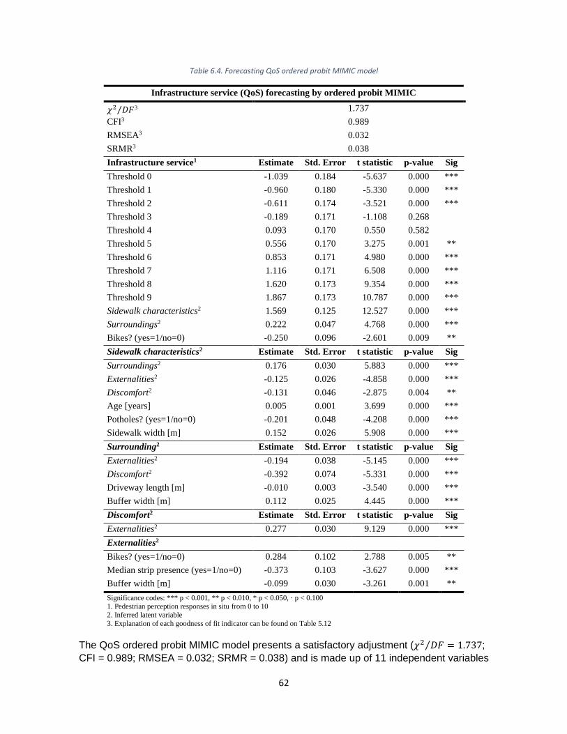
62

Table 6.4. Forecasting QoS ordered probit MIMIC model

Infrastructure service (QoS) forecasting by ordered probit MIMIC

𝜒2 𝐷𝐹⁄ 3 1.737

CFI3 0.989

RMSEA3 0.032

SRMR3 0.038

Infrastructure service1 Estimate Std. Error t statistic p-value Sig

Threshold 0 -1.039 0.184 -5.637 0.000 ***

Threshold 1 -0.960 0.180 -5.330 0.000 ***

Threshold 2 -0.611 0.174 -3.521 0.000 ***

Threshold 3 -0.189 0.171 -1.108 0.268

Threshold 4 0.093 0.170 0.550 0.582

Threshold 5 0.556 0.170 3.275 0.001 **

Threshold 6 0.853 0.171 4.980 0.000 ***

Threshold 7 1.116 0.171 6.508 0.000 ***

Threshold 8 1.620 0.173 9.354 0.000 ***

Threshold 9 1.867 0.173 10.787 0.000 ***

Sidewalk characteristics2 1.569 0.125 12.527 0.000 ***

Surroundings2 0.222 0.047 4.768 0.000 ***

Bikes? (yes=1/no=0) -0.250 0.096 -2.601 0.009 **

Sidewalk characteristics2 Estimate Std. Error t statistic p-value Sig

Surroundings2 0.176 0.030 5.883 0.000 ***

Externalities2 -0.125 0.026 -4.858 0.000 ***

Discomfort2 -0.131 0.046 -2.875 0.004 **

Age [years] 0.005 0.001 3.699 0.000 ***

Potholes? (yes=1/no=0) -0.201 0.048 -4.208 0.000 ***

Sidewalk width [m] 0.152 0.026 5.908 0.000 ***

Surrounding2 Estimate Std. Error t statistic p-value Sig

Externalities2 -0.194 0.038 -5.145 0.000 ***

Discomfort2 -0.392 0.074 -5.331 0.000 ***

Driveway length [m] -0.010 0.003 -3.540 0.000 ***

Buffer width [m] 0.112 0.025 4.445 0.000 ***

Discomfort2 Estimate Std. Error t statistic p-value Sig

Externalities2 0.277 0.030 9.129 0.000 ***

Externalities2

Bikes? (yes=1/no=0) 0.284 0.102 2.788 0.005 **

Median strip presence (yes=1/no=0) -0.373 0.103 -3.627 0.000 ***

Buffer width [m] -0.099 0.030 -3.261 0.001 **


2. Inferred latent variable

3. Explanation of each goodness of fit indicator can be found on Table 5.12

The QoS ordered probit MIMIC model presents a satisfactory adjustment (𝜒2 𝐷𝐹⁄ = 1.737;

CFI = 0.989; RMSEA = 0.032; SRMR = 0.038) and is made up of 11 independent variables

63

and 14 indicators of the latent variables. From the independent variables there are four

latent variables and seven objective attributes. The perceived QoS is positively influenced

by two latent variables (sidewalk characteristics and surroundings) and is negatively

affected by the presence of bicycles. The sidewalk characteristics is improved by the effect

of the surrounding, by the age of the pedestrians using the sidewalk, and by increasing the

sidewalk width. On the other hand, the sidewalk characteristics value decreases with the

presence of potholes in the sidewalk and with the effect of two latent variables

(externalities and discomfort). The surroundings is improved only by increasing the buffer

width. On the other hand, the surroundings decreases by increasing driveway length and

by the effect of two latent variables (externalities and discomfort). Discomfort is one of the

latent variables that decreases the perceived QoS and its effects are aggravated by the

influence of the externalities. Finally, externalities decreases the perceived QoS and its

effects can be mitigated by increasing the buffer width and by the presence of a median

strip. However, its effects can be aggravated by the presence of bicycles on the sidewalk

(see Table 6.4).

Two different approaches were followed to develop the forecasting process for each

sidewalk. The first was to calculate the perceived SQoS for each sidewalk by predicting

the QoS for different users of each sidewalk. Once this was done, the mean of these

values was calculated and was defined as the SQoS. The second approach was to

calculate the perceived SQoS using the mean of the different independent variables of

each sidewalk.

For the first approach, the perceived QoS for each pedestrian from a group of pedestrians

using each one of the sidewalks was calculated first. This calculation was done by

applying the four previously described models and was defined as QoSij for each

pedestrian i using sidewalk j. Then, from the QoSij, and using Equation (16), the mean of

the different pedestrians’ predictions for each sidewalk was calculated to obtain the SQoS

(𝑆𝑄𝑜𝑆𝑚𝑝𝑗).

𝑆𝑄𝑜𝑆𝑚𝑝𝑗=∑ 𝑄𝑜𝑆𝑖𝑗𝑛𝑖=1

𝑛 (16)

The results obtained from the first approach using the four different models described

previously can be found in Table 6.5.

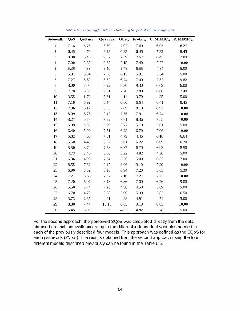
64

Table 6.5. Forecasting for sidewalk QoS using the pedestrian mean approach

Sidewalk QoS QoS min QoS max OLSm Probitm C. MIMICm P. MIMICm

1 7.18 5.76 8.60 7.02 7.60 6.03 6.27

2 6.45 4.78 8.13 6.33 6.45 7.32 8.45

3 8.00 6.43 9.57 7.39 7.67 6.45 7.89

4 7.00 5.65 8.35 7.15 7.40 7.77 10.00

5 5.36 4.33 6.40 5.78 6.55 4.84 5.00

6 5.91 3.84 7.98 6.13 5.91 5.54 5.00

7 7.27 5.82 8.72 6.74 7.00 7.52 9.82

8 8.00 7.08 8.92 8.30 9.30 6.09 6.00

9 7.70 6.39 9.01 7.20 7.80 6.60 7.40

10 3.55 1.79 5.31 4.14 3.70 4.35 5.00

11 7.18 5.92 8.44 6.80 6.64 6.41 8.45

12 7.36 6.17 8.55 7.09 8.18 8.93 10.00

13 8.09 6.76 9.42 7.55 7.91 6.74 10.00

14 8.27 6.73 9.82 7.81 8.36 7.55 10.00

15 5.09 3.39 6.79 5.27 5.18 5.61 5.00

16 6.40 5.09 7.71 6.28 6.70 7.06 10.00

17 5.82 4.03 7.61 4.79 4.45 6.18 6.64

18 5.50 4.48 6.52 5.61 6.22 6.09 6.20

19 5.50 3.72 7.28 6.37 6.70 6.93 8.50

20 4.73 3.46 6.00 5.22 4.82 4.30 5.00

21 6.36 4.98 7.74 5.26 5.00 6.32 7.00

22 8.55 7.62 9.47 8.06 9.10 7.29 10.00

23 6.90 5.52 8.28 6.94 7.20 5.65 5.30

24 7.27 6.68 7.87 7.16 7.27 7.22 10.00

25 7.20 5.97 8.43 6.86 7.00 6.76 9.00

26 5.50 3.74 7.26 4.86 4.50 5.69 5.00

27 6.70 4.72 8.68 5.96 5.90 5.82 6.50

28 3.73 2.85 4.61 4.88 4.91 4.74 5.00

29 8.80 7.44 10.16 8.65 9.10 8.65 10.00

30 5.45 3.95 6.96 4.53 4.82 5.78 5.00

For the second approach, the perceived SQoS was calculated directly from the data

obtained on each sidewalk according to the different independent variables needed in

each of the previously described four models. This approach was defined as the SQoS for

each j sidewalk (𝑆𝑄𝑜𝑆𝑗). The results obtained from the second approach using the four

different models described previously can be found in the Table 6.6.

65

Table 6.6. Forecasting for sidewalk QoS using the sidewalk data

Sidewalk QoS QoS min QoS max OLS Probit C. MIMIC P. MIMIC

1 7.18 5.76 8.60 7.03 7.03 6.03 5.93

2 6.45 4.78 8.13 6.33 6.61 7.32 6.61

3 8.00 6.43 9.57 7.35 7.40 6.45 6.47

4 7.00 5.65 8.35 7.32 7.62 7.77 8.15

5 5.36 4.33 6.40 5.78 6.11 4.84 5.35

6 5.91 3.84 7.98 6.13 5.83 5.54 5.36

7 7.27 5.82 8.72 6.74 6.88 7.52 7.52

8 8.00 7.08 8.92 8.30 8.81 6.09 5.85

9 7.70 6.39 9.01 7.20 7.40 6.60 6.34

10 3.55 1.79 5.31 4.03 3.90 4.36 4.46

11 7.18 5.92 8.44 6.80 6.77 6.41 6.56

12 7.36 6.17 8.55 7.09 7.68 8.93 8.33

13 8.09 6.76 9.42 7.55 7.86 6.74 6.98

14 8.27 6.73 9.82 7.81 8.15 7.55 7.59

15 5.09 3.39 6.79 5.27 5.23 5.61 5.16

16 6.40 5.09 7.71 6.28 6.47 7.06 6.99

17 5.82 4.03 7.61 4.79 4.85 6.18 6.15

18 5.50 4.48 6.52 5.54 6.22 6.09 5.99

19 5.50 3.72 7.28 6.37 6.09 6.93 6.75

20 4.73 3.46 6.00 5.22 5.03 4.30 4.46

21 6.36 4.98 7.74 5.26 5.01 6.32 6.14

22 8.55 7.62 9.47 7.93 8.42 7.29 7.54

23 6.90 5.52 8.28 6.94 6.97 5.65 5.75

24 7.27 6.68 7.87 7.16 7.14 7.22 7.07

25 7.20 5.97 8.43 6.86 6.71 6.76 6.82

26 5.50 3.74 7.26 5.21 5.24 5.70 5.45

27 6.70 4.72 8.68 5.96 5.60 5.82 5.99

28 3.73 2.85 4.61 4.88 4.95 4.74 4.68

29 8.80 7.44 10.16 8.65 8.99 8.65 8.16

30 5.45 3.95 6.96 4.53 4.81 5.78 5.64

Once the two different approaches were computed, a 95% confidence interval of the SQoS

was calculated from the pedestrian survey answers to compare with the forecasting

approaches (see Table 6.5 and Table 6.6). For the cases where the forecasting values

were within the calculated confidence interval for each sidewalk, a score of 1 was

assigned. Otherwise, a score of 0 was assigned. All the sidewalks were predicted and

rated using this procedure and the results are presented in Figure 6.2.

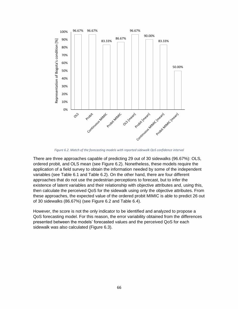
66

Figure 6.2. Match of the forecasting models with reported sidewalk QoS confidence interval

There are three approaches capable of predicting 29 out of 30 sidewalks (96.67%): OLS,

ordered probit, and OLS mean (see Figure 6.2). Nonetheless, these models require the

application of a field survey to obtain the information needed by some of the independent

variables (see Table 6.1 and Table 6.2). On the other hand, there are four different

approaches that do not use the pedestrian perceptions to forecast, but to infer the

existence of latent variables and their relationship with objective attributes and, using this,

then calculate the perceived QoS for the sidewalk using only the objective attributes. From

these approaches, the expected value of the ordered probit MIMIC is able to predict 26 out

of 30 sidewalks (86.67%) (see Figure 6.2 and Table 6.4).

However, the score is not the only indicator to be identified and analyzed to propose a

QoS forecasting model. For this reason, the error variability obtained from the differences

presented between the models’ forecasted values and the perceived QoS for each

sidewalk was also calculated (Figure 6.3).

96.67% 96.67%

83.33%86.67%

96.67%

90.00%

83.33%

50.00%

0%

10%

20%

30%

40%

50%

60%

70%

80%

90%

100%

Rep

rese

nta

tio

n o

f B

ogo

ta's

co

nd

itio

n [

%]

67

Figure 6.3. Sidewalks forecasting models’ errors boxplot

Concerning errors, almost all the proposed models present an error variability of around

0% with a median close to 0. However, there are three approaches with a smaller less

error variability and without outliers: OLS, Probit, and OLS mean. Nonetheless, these

models require the application of a field survey to obtain the information needed by some

of the independent variables (see Table 6.1 and Table 6.2). Of the approaches that do not

need a survey applied, the expected value of the ordered probit MIMIC approach has the

lowest interquartile range which means less variation in the errors (see Figure 6.3).

Finally, a 𝜒2 test was also proposed to verify if the distribution of the frequencies obtained

using the different models were statistically similar to the distribution of the observed data

frequency. The 𝜒2 test presents problems when the frequencies of the categories are less

than 5. For this reason, to carry out this analysis four different categories were created for

the SQoS (5 or less, 6, 7, 8 or more). The calculated test statistic must be compared with

the critical value of 𝜒2 for a significance level of 0.05 and three degrees of freedom (𝜒2 =

7.815). The results for each approach are presented in Table 6.7.

Table 6.7. Statistical values of the 𝜒2 test for sidewalk QoS forecasting

Model approach 𝝌𝟐 statistical value

OLS 1.543

Probit 1.167

Continuous MIMIC 3.848

Probit MIMIC 1.281

OLS [mean] 1.543

Probit [mean] 4.944

Continuous MIMIC [mean] 3.848

Probit MIMIC [mean] 19.083

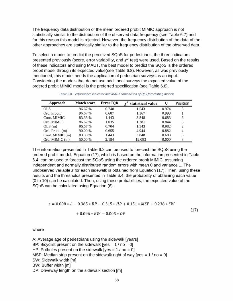
68

The frequency data distribution of the mean ordered probit MIMIC approach is not

statistically similar to the distribution of the observed data frequency (see Table 6.7) and

for this reason this model is rejected. However, the frequency distribution of the data of the

other approaches are statistically similar to the frequency distribution of the observed data.

To select a model to predict the perceived SQoS for pedestrians, the three indicators

presented previously (score, error variability, and 𝜒2 test) were used. Based on the results

of these indicators and using MAUT, the best model to predict the SQoS is the ordered

probit model through its expected value(see Table 6.8). However, as was previously

mentioned, this model needs the application of pedestrian surveys as an input.

Considering the models that do not use additional surveys the expected value of the

ordered probit MIMIC model is the preferred specification (see Table 6.8).

Table 6.8. Performance indicator and MAUT comparison of QoS forecasting models

Approach Match score Error IQR 𝝌𝟐 statistical value U Position

OLS 96.67 % 0.740 1.543 0.974 3

Ord. Probit 96.67 % 0.687 1.167 0.993 1

Cont. MIMIC 83.33 % 1.443 3.848 0.683 6

Ord. MIMIC 86.67 % 1.035 1.281 0.844 5

OLS (m) 96.67 % 0.704 1.543 0.982 2

Ord. Probit (m) 90.00 % 0.655 4.944 0.882 4

Cont. MIMIC (m) 83.33 % 1.443 3.848 0.683 6

Ord. MIMIC (m) 50.00 % 2.184 19.083 0.000 8

The information presented in Table 6.2 can be used to forecast the SQoS using the

ordered probit model. Equation (17), which is based on the information presented in Table

6.4, can be used to forecast the SQoS using the ordered probit MIMIC, assuming

independent and normally distributed random errors with mean 0 and variance 1. The

unobserved variable z for each sidewalk is obtained from Equation (17). Then, using these

results and the thresholds presented in Table 6.4, the probability of obtaining each value

(0 to 10) can be calculated. Then, using these probabilities, the expected value of the

SQoS can be calculated using Equation (6).

𝑧 = 0.008 ∗ 𝐴 − 0.365 ∗ 𝐵𝑃 − 0.315 ∗ 𝐻𝑃 + 0.151 ∗ 𝑀𝑆𝑃 + 0.238 ∗ 𝑆𝑊

+ 0.096 ∗ 𝐵𝑊 − 0.005 ∗ 𝐷𝑃 (17)

where

A: Average age of pedestrians using the sidewalk [years]

BP: Bicyclist present on the sidewalk [yes = 1 / no = 0]

HP: Potholes present on the sidewalk [yes = 1 / no = 0]

MSP: Median strip present on the sidewalk right of way [yes = 1 / no = 0]

SW: Sidewalk width [m]

BW: Buffer width [m]

DP: Driveway length on the sidewalk section [m]

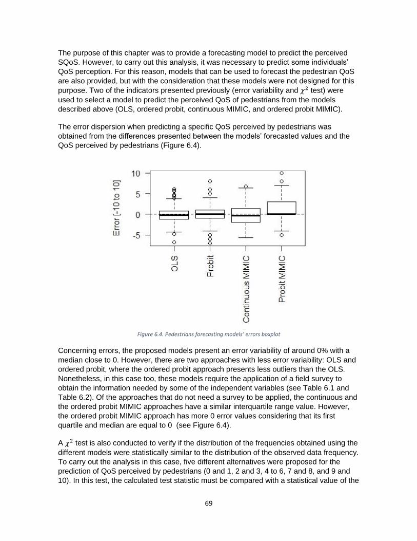
69

The purpose of this chapter was to provide a forecasting model to predict the perceived

SQoS. However, to carry out this analysis, it was necessary to predict some individuals’

QoS perception. For this reason, models that can be used to forecast the pedestrian QoS

are also provided, but with the consideration that these models were not designed for this

purpose. Two of the indicators presented previously (error variability and 𝜒2 test) were

used to select a model to predict the perceived QoS of pedestrians from the models

described above (OLS, ordered probit, continuous MIMIC, and ordered probit MIMIC).

The error dispersion when predicting a specific QoS perceived by pedestrians was

obtained from the differences presented between the models’ forecasted values and the

QoS perceived by pedestrians (Figure 6.4).

Figure 6.4. Pedestrians forecasting models’ errors boxplot

Concerning errors, the proposed models present an error variability of around 0% with a

median close to 0. However, there are two approaches with less error variability: OLS and

ordered probit, where the ordered probit approach presents less outliers than the OLS.

Nonetheless, in this case too, these models require the application of a field survey to

obtain the information needed by some of the independent variables (see Table 6.1 and

Table 6.2). Of the approaches that do not need a survey to be applied, the continuous and

the ordered probit MIMIC approaches have a similar interquartile range value. However,

the ordered probit MIMIC approach has more 0 error values considering that its first

quartile and median are equal to 0 (see Figure 6.4).

A 𝜒2 test is also conducted to verify if the distribution of the frequencies obtained using the

different models were statistically similar to the distribution of the observed data frequency.

To carry out the analysis in this case, five different alternatives were proposed for the

prediction of QoS perceived by pedestrians (0 and 1, 2 and 3, 4 to 6, 7 and 8, and 9 and

10). In this test, the calculated test statistic must be compared with a statistical value of the

70

𝜒2 with a significance level of 0.05 and four degrees of freedom (𝜒2 = 9.488), to accept or

reject the null hypothesis. The results of the test statistic for each approach are presented

in Table 6.9.

Table 6.9. Statistical values of the 𝜒2 test for pedestrian QoS forecasting

Model approach 𝝌𝟐 statistical value

OLS 136.649

Probit 3.136

Continuous MIMIC 388.839

Probit MIMIC 116.743

Only the ordered probit approach can be considered to have a frequency distribution of the

expected data that is statistically similar to the frequency distribution of the observed data

(see Table 6.9). In addition, for the reason previously presented all the other models have

to be rejected. The only accepted approach requires the application of a field survey to

obtain the information needed by some of the independent variables (see Table 6.2). In

addition, to ask about the perceived QoS for an individual pedestrian using the ordered

probit, needs to consider a regrouped scale (0 and 1, 2 and 3, 4 to 6, 7 and 8, and 9 and

10) to be answered for the surveyed.

71

7. Discussion and analysis The oldest, most widely accepted, and most popular service indicator is the LOS. Initially,

LOS methods (developed for motorized traffic) considered only attributes related to the

flow-capacity relationship (Roess & Prassas, 2014; Transportation Research Board, 1965).

The first methodologies developed to calculate PPSI were based on the LOS indicator that

considered only on-site measurable attributes related to the flow-capacity relationship. In

the following years, it evolved into a new manner that considered other on-site measurable

attributes, creating methodologies with better PPSI predictive power. Then, the most-

recently proposed evolution is that which considers the perceptions of experts to calculate

the perceived PPSI (see Table 4.5). However, expert judgement-based methodologies

appear least in the literature, despite having the best PPSI predictive power (see Table

4.5). For this reason, considering the users’ (pedestrians’) perceptions for methodologies

that try to explain or predict the QoS can result in better transportation infrastructures for

pedestrians.

The results strongly suggest that PPSI methodologies are site-specific. The poor

performance in explaining the perceived QoS (maximum 50% of the locations) suggest

that methods need to be calibrated for the specific town or city. In fact, the official PLOS

method for Bogota (Alcaldia Mayor de Bogota D.C., 2005) which is a calibrated version of

the method used by the Transportation Research Board (2000) increases its performance

by 23.34 percentage points because of this calibration (see Table 4.4). All the

methodologies used for this study were developed to evaluate the PPSI on the sidewalk

link without considering their intersections. Out of the 28 methodologies evaluated in the

30 locations in Bogotá, 22 of them use objective measurable variables. Out of these 22,

36% use attributes related to the flow-capacity relationship and so data can be gathered

from a short visit to where the different tallies have to be made. The remaining 64% use

objective attributes of the sidewalk and their surroundings, where most of the information

needed can be gathered from on-site measurements. There are six methodologies that

need the evaluation of experts or subjective information about the sidewalks to be applied.

The user perception inputs are one of the least studied in terms of its capacity to explain

the QoS perception by pedestrians, despite the fact that perception variables contribute

most to the variance explanation of the perceived QoS (see Figure 5.1, Figure 5.2, Figure

5.3, and Figure 5.4). This result matches that outlined by Fernández-Heredia et al. (2016)

in terms of improving the chosen model’s performance by considering perceptions. In this

study, it can be suggested that when perceptual variables are not considered, the models’

performance in terms of variance explanation decreases sharply in comparison with the

models containing user-perception variables (see Figure 5.1, Figure 5.2, Figure 5.3, and

Figure 5.4). In addition, the results suggest that perceptual variables explain more

variance in the perceived QoS, regardless of the grouping decision or the order of addition

of perceptions to the models, as they variance explanation never overlap the other

variables’ variance explanation (see Table 5.3, Table 5.5, and Table 5.7).

The other groups of variables used to explain the perceived QoS, namely environmental,

sociodemographic, and physical variables, have a lower contribution to the variance

explanation of the perceived QoS in comparison with the perceptual group of variables. In

addition, in terms of perceived QoS variance explanation, there are no differences

72

between these group of variables. Initially, the variance explanation of the perceived QoS

of the physical and sociodemographic variables overlap when they are used as

independent variables (see Table 5.6 and Table 5.7). However, the maximum variance

explanation value generated by the use of the physical variables is greater than that

generated by the sociodemographic variables (see Table 5.6), which supports the idea

that comparing these two groups of variables the methodologies for the calculation of PPSI

based on physical sidewalk attributes are better (see Table 4.5). In addition, the

overlapping of the variance explanation can be also seen when the sociodemographic and

environmental attributes’ values are compared (see Table 5.6 and Table 5.7). In this case,

the maximum variance explanation value generated by the use of sociodemographic

attributes is greater than that generated by the environmental attributes (see Table 5.6).

However, this overlapping is significantly different from the physical and perceptual

attributes’ values, which means that sociodemographic and environmental groups of

variables can be considered to contribute less to the variance explanation of the perceived

QoS when the other group of inputs play a part in the explanation (see Table 5.7).

Considering the power of users’ perceptions to explain the perceived QoS, much more

information can be extracted and analyzed from perceptions to better understand QoS. To

uncover latent variables from users’ perceptions is an approach that identifies the

intangible variables’ influence on the perceptions (Ortúzar & Willumsen, 2011). The first

step in proposing the existence of latent variables is to develop an exploratory factor

analysis (EFA). The advantage of using EFA is the possibility of determining which

perception attributes share common variance-covariance characteristics. Then, using a

confirmatory factor analysis (CFA) the hypothesis developed from the EFA can be tested

to confirm the existence of a latent variable and its perception indicators (Schumacker &

Lomax, 2004). For this study, it is possible to specify the number of latent variables and

indicators from the CFA results to identify a theoretical model that can be used or applied

in different contexts. A very recent paper by Geetha Rajendran Bivina & Parida (2019)

provided a latent variable approach based on user perceptions that identified four latent

variables that positively influence the PLOS. The results of the present research also

identified the positive effects discovered by Geetha Rajendran Bivina & Parida (2019), but

in addition, identified three latent variables that negatively influence the perceived QoS.

There are two latent variables that are initially perceived by pedestrians when walking that

affects their perception of the QoS: bike hassles and amenities (see Figure 5.5). The bike

hassles explains the pedestrians’ perception of bike speed and flow in both directions (see

Table 5.11). In the literature it can be found that the interaction of pedestrians with bicycles

on their infrastructure decreases the QoS that an infrastructure renders (Muraleetharan et

al., 2005; Muraleetharan & Hagiwara, 2007; Sahani et al., 2017). However, the negative

impact generated by the bike hassles on the perceived QoS is not direct, and needs the

mediation of other latent variables (see Figure 5.5). On the other hand, the amenities

explains the pedestrian’s perception of the presence of restrooms, shops, and shade on

the sidewalk, positively impacting the perceived QoS through the mediation of other latent

variables. This result is supported in the literature, where it is established that the

presence and good quality of public restrooms on sidewalks positively impacts the

amenities, generating a better QoS for a sidewalk (Motamed & Bitaraf, 2016). In addition,

the presence of shops on the infrastructure or close to the infrastructure provide a safe

and secure sidewalk (Motamed & Bitaraf, 2016) where people are more likely to walk

73

(Choi et al., 2016; Pikora et al., 2003). Finally, the presence of shade on the sidewalks

also contributes to an increase in pedestrian comfort when walking (Jaskiewicz, 1999) and

improves the visual quality of the environment (Macdonald et al., 2018).

Externalities helps to mediate the effect of bike hassles and amenities on the perceived

QoS. This latent variable explains the pedestrian’s perception of the road width, number of

vehicular lanes, HGV flow, vehicular speed, and noise, negatively impacting the perceived

QoS through the mediation of other latent variables (see Table 5.11 and Figure 5.5). This

result is supported in the literature, where it is explained that the interaction of pedestrians

with traffic attributes like heavy goods vehicle (HGV) flow generate an increase in stress

levels, decreasing the pedestrian LOS (Mozer, 1994). In addition, when pedestrians

interact with high vehicular speeds, an increase in stress levels is also evidenced which

affects their experience (Mozer, 1994), decreasing the perceived pedestrian safety

(Jaskiewicz, 1999; Landis et al., 2001; Motamed & Bitaraf, 2016; State of Florida

Department of Transportation, 2009; Talavera-Garcia & Soria-Lara, 2015), PLOS (S. Kim

et al., 2013; Landis et al., 2001; Mozer, 1994; Sahani et al., 2017; State of Florida

Department of Transportation, 2009), level of comfort (Pikora et al., 2003), and satisfaction

(Jensen, 2007). The literature also mentions that vehicle infrastructure characteristics like

wide roads and a high number of lanes increase pedestrian stress levels (Macdonald et

al., 2018; Mozer, 1994), and decrease pedestrian satisfaction (Choi et al., 2016; Jensen,

2007). However, these interactions do not take place only between pedestrians and

geometric and traffic variables, there is also an interaction with noise levels on the

sidewalk that decreases perceived pedestrian pleasure (Motamed & Bitaraf, 2016), the

QoS for pedestrians (Sarkar, 2003) and the PLOS (Christopoulou & Pitsiava-Latinopoulou,

2012) when the noise level increases.

One of the latent variables that helps to mediate the negative effect of externalities on the

perceived QoS is the discomfort. This latent variable explains the pedestrian’s perception

of interaction with other pedestrians and the perceived stress on the infrastructure,

negatively impacting the perceived QoS through the mediation of other latent variables

(see Table 5.11 and Figure 5.5). This result is supported by the literature, which states

that, over time, pedestrian interaction with other pedestrians decreases their PLOS (Asadi-

Shekari et al., 2013; Banerjee et al., 2018). In addition, stress levels are understood to

move in the opposite direction to the PLOS. In other words, when stress levels go up, the

PLOS goes down (Mozer, 1994).

Another latent variable that helps to mediate the effect of discomfort, externalities, bike

hassles, and amenities on the perceived QoS is protection. This latent variable explains

the pedestrian’s perception of protection in terms of safety and security on a sidewalk, and

it positively impacts the perceived QoS through the mediation of other latent variables (see

Table 5.11 and Figure 5.5). This result is supported in the literature, where it was found

that increasing the level of safety (Christopoulou & Pitsiava-Latinopoulou, 2012; Ewing et

al., 2006; Pikora et al., 2003) and security (G. R. Bivina et al., 2018; Gallin, 2001;

Motamed & Bitaraf, 2016) also increased pedestrian QoS.

Similarly, the surroundings also helps to mediate the effect of protection, discomfort, and

externalities on the perceived QoS. This latent variable explains the pedestrian’s

perception of the weather, lighting, odor, environment, cleanliness, and landscape present

on a sidewalk, and positively impacts the perceived QoS both directly and through the

74

mediation of the sidewalk characteristics (see Table 5.11 and Figure 5.5). This result is

supported in the literature, where it is initially explained that bad weather conditions like

rain can cause pedestrians to express negative attitudes (Kang & Fricker, 2016). In

addition, the improvement of built environment characteristics like a good sidewalk

environment and landscape increases the perceived pedestrian comfort (T. Kim et al.,

2011) and satisfaction (Jensen, 2007). The literature also mentions that there are some

characteristics of the sidewalk surroundings like good lighting that also increases the

perceived sidewalk PLOS (Kang et al., 2013). In addition, having a clean sidewalk with a

pleasant odor can also increase the quality of the sidewalk (Motamed & Bitaraf, 2016;

Pikora et al., 2003) and improve the pleasure experienced by pedestrians (G. R. Bivina et

al., 2018).

Finally, the sidewalk characteristics also helps to mediate the effect of surroundings,

protection, discomfort, and externalities on the perceived QoS. This latent variable

explains the pedestrian’s perception of the sidewalk width, condition, furniture, trees,

signage, and the public transport access, directly and positively impacting the perceived

QoS (see Table 5.11 and Figure 5.5). These results are supported in the literature, which

state that, over time, an increase in the width of a sidewalk increases PLOS (Asadi-

Shekari et al., 2013; Banerjee et al., 2018). However, this geometry attribute is not the only

one to consider when trying to understand the sidewalk QoS by considering the sidewalk

characteristics. The interaction of pedestrians with elements of the sidewalk like the

presence of good furniture improve pedestrian comfort (Sarkar, 2003) and pleasure

(Motamed & Bitaraf, 2016) when walking. In addition, the presence of trees on the

sidewalk increases pedestrian satisfaction (Jensen, 2007), PLOS (Christopoulou &

Pitsiava-Latinopoulou, 2012; Talavera-Garcia & Soria-Lara, 2015), and generate a more

attractive infrastructure for walking (Choi et al., 2016; Motamed & Bitaraf, 2016). Also, the

presence of good pedestrian signaling and support facilities that aid pedestrians increase

the PLOS (Gallin, 2001) and sidewalk QoS (T. Kim et al., 2011). However, the fact that

sidewalks have the previously mentioned elements is not enough, they, and the sidewalk,

must also be in good condition to provide a better infrastructure for pedestrians (G. R.

Bivina et al., 2018; Christopoulou & Pitsiava-Latinopoulou, 2012; Gallin, 2001; Jaskiewicz,

1999; T. Kim et al., 2011; Marisamynathan & Lakshmi, 2016; Motamed & Bitaraf, 2016;

Pikora et al., 2003; Sarkar, 2003). Lastly, the access to public transport on a sidewalk also

increases the sidewalk PLOS (Christopoulou & Pitsiava-Latinopoulou, 2012) and

satisfaction (Choi et al., 2016), providing a more attractive sidewalk to walk on (Pikora et

al., 2003).

All the previously mentioned effects, both direct and mediated, affect the pedestrian

perception of the QoS when walking. There are four different latent variables that generate

a positive effect on the perceived QoS: sidewalk characteristics, surroundings, protection,

and amenities. Of these latent variables, the one that generates the greatest positive effect

on the perceived QoS is sidewalk characteristics. This effect is direct only and is

understandable because this latent variable relates to the direct interaction of the

pedestrian with the infrastructure. However, in order to increase the perception of the QoS

is not enough to provide a sidewalk with good characteristics. It is also necessary to build

a sidewalk where pedestrians can perceive good surroundings, protection against crime

and accidents, and the presence of places to interact with. On the other hand, there are

three different latent variables that negatively impact the perceived QoS: discomfort,

75

externalities, and bike hassles. In general, these three latent variables express the way

that pedestrians interact with other transportation modes including other pedestrians. The

externalities, which considers the interaction of pedestrians with non-active modes,

generates the greatest negative effect on the perceived QoS. Then, discomfort, which

considers the interaction of pedestrians with other pedestrians, generates the second

greatest negative effect on the perceived QoS. Finally, bike hassles which considers the

interaction of pedestrians with cyclists, generates the lowest negative effect on the

perceived QoS (see Table 5.14).

The previous paragraphs explain the ways in which pedestrians perceive the QoS when

walking on an urban sidewalk by considering their perceptions. This knowledge can

contribute to understanding why and how pedestrians quantify the QoS. However, it is also

useful for knowing which user and sidewalk attributes have effects on the perceived

sidewalk QoS (SQoS). To select a forecasting model for the perceived SQoS and QoS,

three different performance indicators were used: match score, error variability, and the 𝜒2

test. As was mentioned in the previous chapter, the model selected was the expected

value of the ordered probit to predict the perceived SQoS and QoS (Table 6.2). However,

because of the difficulties applying this model to real-life conditions due to the need to

carry out surveys, the expected value of the ordered probit MIMIC model was also

selected to calculate only the perceived SQoS (Table 6.4). In addition, the choice of the

ordered models like the ones selected is also supported in the literature where the use of

this approximation is suggested for trying to understand the QoS (Eboli & Mazzulla, 2010).

In both cases, for sidewalk forecasting, the expected value of each model was selected

because the SQoS is considered to be a continuous value. In the case of the perceived

QoS forecasting the ordered probit model is used to select the most probable value as the

perceived QoS.

Considering the forecasting ordered probit model, 16 independent variables were identified

that contribute to the prediction of the SQoS and the perceived QoS. From these

independent variables, 11 are users’ perceptions and only five are characteristics of the

users and sidewalks. This finding is not surprising because the literature manifests that the

models’ performance improves when users’ perceptions are included in them (Fernández-

Heredia et al., 2016). Some of the perception independent variables improve the perceived

SQoS and QoS that consider how positively pedestrians perceive sidewalk elements

(sidewalk surface condition, horizontal marking, sidewalk furniture, organized spaces, and

tree presence), the sidewalk surroundings (building articulation, road safety, and lighting),

and geometry aspects of the sidewalk (sidewalk width). On the other hand, there are also

perceptual independent variables that decrease the perceived SQoS and QoS that

considers the pedestrians’ irritation caused by other transportation modes (heavy good

vehicles and vehicular flow close to pedestrians). Considering the independent variables

consisting of characteristics of the sidewalk, this model suggests that providing bus stops

and restrooms on sidewalks increases the perceived SQoS and QoS. On the other hand,

on sidewalks where the length of driveways and noise increase, the perception of the

SQoS and QoS decrease. Finally, considering user characteristics as independent

variables, this model suggests that the older the user, the better the perception of the

SQoS and QoS (see Table 6.2).

76

From the ordered probit model the contribution of objective and subjective independent

variables to the QoS forecasting can be compared. The absolute effect of the subjective

independent variables on the unobserved value z represents 65% of the total effect and

the remaining 35% of the effect it is attributed to the objective independent variables. This

effect is similar to that found when comparing the variability explanation of the perceived

QoS using perceptions. Additionally, the necessity of including perceptions to increase

understanding of pedestrian perception of the QoS when walking is reinforced.

Turning to the forecasting ordered probit MIMIC model, 11 independent variables that

contribute to the prediction of the SQoS were identified. Of these independent variables, 7

are user and sidewalk characteristics. In addition, 4 are latent variables that were

previously discussed and analyzed (sidewalk characteristics, surroundings, discomfort,

and externalities). The use of latent variables in these kinds of models allows this

phenomenon to be approached with the consideration of both the objective and subjective

variables (Eboli & Mazzulla, 2015). In this case, using the sidewalk and user

characteristics each latent variable and subsequently the perceived SQoS are explained

(see Table 6.4).

The externalities is the first to be perceived by pedestrians when walking, negatively

impacting the perceived SQoS with the mediation of the other latent variables (discomfort,

surroundings, and sidewalk characteristics). To predict the value of this latent variable, the

ordered probit MIMIC model suggests that sidewalks with the presence of bicyclists

increases the latent variable value, decreasing the perceived SQoS. This suggestion is

supported in the literature, where it is established that the presence of bicycles on

sidewalks negatively impact the perceived PLOS (Dandan et al., 2007; Kang et al., 2013).

In addition, this model also suggests that sidewalks located along rights of way and that

have a median strip which increases the separation between pedestrians and motor

vehicles can counteract the effects of the externalities on the perceived SQoS. These

results are supported in the literature where it is established that the presence of a median

strip along the right of way improves the satisfaction of pedestrians because of the

controlling effect of this element on the motor vehicles (Jensen, 2007). In addition, an

increase in the separation between pedestrians and motor vehicles has been identified

over time to have an effect that improves the PLOS (Asadi-Shekari et al., 2013; Banerjee

et al., 2018).

The second latent variable that the ordered probit MIMIC model suggests that pedestrians

perceive when walking is discomfort. This latent variable also negatively impacts the

perceived SQoS with the mediation of other latent variables (surroundings and sidewalk

characteristics). This latent variable is impacted by the externalities, which means that the

sidewalk characteristics affecting the externalities also indirectly affect the discomfort.

However, the present study was not able to find which sidewalk or user characteristics can

directly impact the value of this latent variable.

The third latent variable that the ordered probit MIMIC model suggests that pedestrians

perceive when walking is surroundings. This latent variable positively and directly impacts

the perceived SQoS and with the mediation of the sidewalk characteristics. In addition, this

latent variable is negatively impacted by the externalities and discomfort, which means that

bike presence, median strip presence, and buffer width indirectly impact this latent

variable. However, the ordered probit MIMIC model suggests that not only the buffer width

77

indirectly impacts this latent variable, but also an increase of the separation between

pedestrians and motor vehicles directly impacts this latent variable and improves its value.

In addition, the ordered probit MIMIC model also suggests that increasing the length of

driveways along the sidewalk decreases the perception of the surroundings for

pedestrians, negatively impacting the perceived SQoS. This result is supported by the

literature, where it is established that the presence of driveway segments increases

conflicts for pedestrians (Gallin, 2001; Petritsch et al., 2006), creates potential dangers for

them (Mozer, 1994), and reduces their satisfaction (Choi et al., 2016), comfort, and safety

(Dandan et al., 2007).

The fourth and last latent variable that the ordered probit MIMIC model suggests that

pedestrians perceive when walking is the sidewalk characteristics. This latent variable also

positively impacts the perceived SQoS and it does so only in a direct way. In addition, this

latent variable is impacted by the other latent variables (surroundings, discomfort, and

externalities). This means that the attributes buffer width, driveway length, median strip

presence, and bike presence indirectly impact this latent variable. In addition, the ordered

probit MIMIC model suggests that some characteristics of the sidewalk like the presence

of potholes can decrease the latent variable value, negatively impacting the perceived

SQoS. This finding can be supported in the literature that states that a sidewalk in bad

condition represented by the presence of potholes decreases the infrastructure quality (G.

R. Bivina et al., 2018; Christopoulou & Pitsiava-Latinopoulou, 2012; Gallin, 2001;

Jaskiewicz, 1999; T. Kim et al., 2011; Marisamynathan & Lakshmi, 2016; Motamed &

Bitaraf, 2016; Pikora et al., 2003; Sarkar, 2003). In addition, this model also suggests that

increasing other sidewalk characteristics like sidewalk width improve the latent variable

value and the perceived SQoS, which is consistent with what has been developed in the

literature over time (Asadi-Shekari et al., 2013; Banerjee et al., 2018). In addition, this

model also suggests that a user characteristic like user age also impacts the latent

variable value in a positive way, which means that the older the user the better the value

for the latent variable and the perceived SQoS.

All the previously mentioned latent variables (sidewalk characteristics, surroundings,

discomfort, and externalities) affect the perceived SQoS both directly and indirectly. This

means that the attribute user age and the sidewalk attributes pothole presence, sidewalk

width, buffer width, driveway length, median strip presence, and bike presence indirectly

affect the perceived SQoS. However, the ordered probit MIMIC model suggests that the

bicyclist presence not only indirectly impacts the perceived SQoS, but also the presence of

bicyclists on the sidewalk directly and negatively impacts the perceived SQoS. In addition,

improving the perception of the sidewalk characteristics and surroundings generates a

positive impact on the perceived SQoS. In addition, removing the nuisances that

pedestrians perceive from discomfort and externalities, also improves the perceived

SQoS. These improvements and neutralizations can be developed by considering and

improving the different sidewalk attributes identified previously (see Table 6.4).

From the results of this study, the performance of different methodologies to calculate

PPSI found in the literature were tested. From this analysis, it was possible to establish

that methodologies using expert judgment to calculate the PPSI better represent the local

conditions of the city of Bogotá (see Table 4.5). However, without proper calibration, the

different methodologies do not perform well when directly applied to the city of Bogotá (see

78

Table 6.5). Nonetheless, the results on the use of perceptions from experts could be used

as a base to continue the research and explore this direction more. The first step was to

establish the role and impact of users’ perceptions when attempting to calculate the

perceived QoS. From this step, it can be suggested that for pedestrians’ QoS the most

important attributes to consider are their perceptions (see Table 5.7). The second step was

to understand how pedestrians perceive their QoS through the development of a perceived

QoS cognitive map (see Table 5.14 and Figure 5.5). Once this cognitive map was

developed it could be used as a tool to understand which of the attributes present when

pedestrians walk on urban sidewalks impact their perception of the QoS. In addition, this

cognitive map also serves as a tool to make choices about what characteristics should be

improved, and how to intervene to improve the perceived QoS. Finally, considering the

importance of users’ perceptions, two models were developed in this study to forecast the

perceived SQoS and QoS (see Table 6.2 and Table 6.4). These models can be used to

define the perceived SQoS of the different sidewalks for the city of Bogotá, with the

consideration of basic entry data about each sidewalk, their users, and their rights of way.

79

8. Conclusions, recommendations,

and further research 8.1 Conclusions Despite the steady and continuous evolution of indicators and methods to evaluate the

service or performance of pedestrian infrastructure, over recent decades, methods have

not been developed into new concepts that improve explanatory and forecasting results.

The fact that expert-judgement methods were proved to produce the best outcomes in

Bogotá, together with the poor performance of the majority of existing methodologies, gave

an insight into the discovery that person-oriented models are quite convenient.

When the PPSI on urban sidewalks must be evaluated using existing methodologies, it is

highly recommended that the methodologies be calibrated for the specific place or context.

This suggestion is based on the results of this study where the Alcaldia Mayor de Bogota

D.C. (2005) methodology was calibrated before its application, generating an increase on

the forecasting ability in comparison with the methodology on which it was based

(Transportation Research Board, 2000) (see Table 4.4).

This dissertation provides solid evidence for the relevance of user input when assessing the service or the performance of a segment (linear) pedestrian infrastructure, which can be added to the models as independent variables (through the development of OLS or ordered models) or as latent variables indicators (through the development of SEM or MIMIC models). Perceptions, which are subjective responses based on different peoples’ answers for the same attribute, substantially increase the explanation of the QoS assigned by pedestrians to an urban sidewalk. Unlike a highway, where drivers care about flow-capacity attributes (speed and delays) that allow them to complete their trip as fast as possible, walkers interact with the open environment, with the city, and with other modes, making the framework for PPSI more complex than for other modes.

A major conclusion of this research is the identification of the sources of QoS on urban

sidewalks. These sources were mapped on a cognitive map that can be used to identify

them clearly. From this cognitive map, four latent variables were found to impact the

perceived QoS in a positive way. It was also established that the pedestrian’s perception

of sidewalk characteristics (latent variable) improves the perceived QoS the most. For this

reason, increasing the quality of the sidewalk characteristics (width, condition, furniture,

trees, public transport access and signage) must be a priority in the improvement of urban

sidewalks. In addition, it is not recommended that the positive effect of other latent

variables be omitted, as these also positively impact the perceived QoS. This means that

to improve the pedestrian infrastructure, perceptions of the surroundings (weather, lighting,

odor, environment, cleanliness, and landscape), protection (security, sidewalk safety and

road safety), and amenities (restrooms, shops, and shade) need also be improved.

On the other hand, three latent variables related to the interaction between pedestrians

and other transportation modes negatively impact the perceived QoS. The first,

externalities, represents the interaction between pedestrians and non-active modes and

has the greatest negative impact on the perceived QoS. Counteracting the negative effect

of externalities on pedestrians should result in an improvement of the perceived QoS. This

counterbalance can be generated in two different ways: (i) by improving the pedestrian’s

80

perception of the amenities (restrooms, shops, and shade), and (ii) by decreasing the

negative effect of this latent variable with the design of rights of way with less space for

non-active vehicles (narrower vehicular roads with less lanes), and regulating the heavy

goods vehicle (HGV) flow, vehicular speed, and noise. However, it is highly recommended

that both counteracting actions are applied simultaneously. In addition, it is also

recommended that the negative impact of the other latent variables related to the

interaction of pedestrians with bicyclists (bike hassles) and with other pedestrians

(discomfort) be also considered. To decrease the negative impact caused by bicyclists, it

is recommended that their flow and speed close to pedestrians be regulated, to improve

the pedestrian’s perceptions of this hassle. In addition, to decrease the negative impact

caused by the interaction between pedestrians themselves (discomfort) the

recommendation is to design and develop more spaces that can be used for walking,

reducing pedestrian density and the potential for conflict between them.

Once the importance of perceptions in the explanation of the perceived QoS was

identified, the next step was to develop a methodology to predict the SQoS for urban

sidewalks in Bogotá. To accomplish this objective, four different approximations (OLS,

ordered probit, continuous MIMIC, and ordered probit MIMIC) were used. The results

recommend the use of ordered models considering that they have better goodness of fit

indicators and reproduce the observed data distribution better. In addition, in the literature,

the ordered models are recommended most highly for service quality investigations.

The resulting forecasting models restate the importance of perceptions in the explanation

of the perceived SQoS and QoS. This affirmation can be supported by fact that the

perceptual independent variables explain the SQoS and QoS variance in the models

better. In addition, the role and impacts of some sidewalk characteristics are suggested by

the forecasting models (see Table 6.2 and Table 6.4). Initially, these models suggested

that the presence of bicyclists on the sidewalk directly impacts the perceived SQoS and

increased the negative effect of externalities in the perceived SQoS. In addition, increasing

the separation between pedestrians and the road directly counteracts the negative effect

of externalities and improves the perception of surroundings. Also, designing rights of way

that include median strips counteracts the negative effect of the externalities on the

perceived SQoS and QoS. Similarly, building sidewalks with reduced driveway length will

impact positively on the perception of surroundings. Also, sidewalks without potholes and

increased width, impact positively on the pedestrian perception of sidewalk characteristics.

In conclusion, it is possible to change on-site attributes and perceptions to generate better

pedestrian infrastructure and to improve the local representation of an SQoS and QoS

model.

8.2 Recommendations and further research Considering that this study was limited, this section will outline some of the

recommendations for developing further research on this topic. Initially, to understand the

complete panorama of the different PPSI and their effects on pedestrians’ impressions, a

study that considers the different ways in which pedestrians perceive the PPSI (comfort,

pleasure, stress, experience, and satisfaction) should be developed. In this research, it is

highly recommended to understand the differences between each element stated by

pedestrians when they are asked to rate each of these terms. For this, a cognitive map

81

explaining how pedestrians understand each term could be also useful for improving

knowledge about pedestrians and how to build better urban sidewalks for them.

In this study two SQoS forecasting methodologies were proposed, however, these

methodologies were designed for Bogotá only. Considering the structure of the ordered

probit MIMIC it is possible to develop a methodology to calibrate this model for its use in a

different context. The first approach for developing this calibration methodology may

consist of understanding the way that the measurement model (users’ perceptions) is

generated in the new context. Then, by considering the differences between the proposed

measurement model and the one in the new context, a calibration method can be

proposed. Also, there are potential in the use of artificial intelligence to obtain the needed

information from images to objectively apply the forecasting methodology.

In addition, the methodology that the present study proposed for the calculation of the

perceived QoS requires pedestrian interception surveys and so this methodology was not

part of the scope of this research. For this reason, it is highly recommended to develop a

latent variable methodology that can be applied using only on-site measurable attributes to

forecast the pedestrian QoS. Once this methodology is proposed, it has to be tested in

terms of goodness of fit indicators and data generation distribution. The purpose of

creating a methodology that can be applied only with on-site measurable attributes is to

speed up the process for practitioners.

Finally, this study makes one of the first attempts to understand pedestrians’ perceptions

and this topic is still nascent. It only provides information about pedestrians considered as

a transportation mode. For this reason, it is recommended that more studies be developed

that contemplate the heterogeneous effects of pedestrians by consider their differences

(e.g., sex, occupation, etc.) and the interactions with their surroundings that can exist

because of these differences.

82

9. References Adkins, A., Dill, J., Luhr, G., & Neal, M. (2012). Unpacking Walkability: Testing the Influence of

Urban Design Features on Perceptions of Walking Environment Attractiveness. Journal of Urban Design, 17(4), 499–510. https://doi.org/10.1080/13574809.2012.706365

Alcaldia Mayor de Bogota D.C. (2005). Manual de Planeacion y Diseño para la Administracion del Transito y el Transporte. Bogota, DC.

Aliman, N. K., Hashim, S. M., Wahid, S. D. M., & Harudin, S. (2016). Tourists’ Satisfaction with a Destination: An Investigation on Visitors to Langkawi Island. International Journal of Marketing Studies. https://doi.org/10.5539/ijms.v8n3p173

Asadi-Shekari, Z., Moeinaddini, M., & Zaly Shah, M. (2013). Non-motorised Level of Service: Addressing Challenges in Pedestrian and Bicycle Level of Service. Transport Reviews, 33(2), 166–194. https://doi.org/10.1080/01441647.2013.775613

Badara, M. S., Kamariah Nik Mat, N., Muhd Mujtaba, A., Nayef Al-Refai, A., Musa Badara, A., & Abubakar, F. M. (2013). Direct Effect of Service Quality Dimensions on Customer Satisfaction and Customer Loyalty in Nigerian Islamic Bank. Management. https://doi.org/10.5923/j.mm.20130301.02

Banerjee, A., Maurya, A. K., & Lämmel, G. (2018). Pedestrian flow characteristics and level of service on dissimilar facilities: A critical review. Collective Dynamics, 3, A17. https://doi.org/10.17815/CD.2018.17

Bezerra, G. C. L., & Gomes, C. F. (2016). Measuring airport service quality: A multidimensional approach. Journal of Air Transport Management. https://doi.org/10.1016/j.jairtraman.2016.02.001

Bivina, G. R., Parida, P., Advani, M., & Parida, M. (2018). Pedestrian level of service model for evaluating and improving sidewalks from various land uses. European Transport - Trasporti Europei, (67), 1–19.

Bivina, Geetha Rajendran, & Parida, M. (2019). Modelling perceived pedestrian level of service of sidewalks: A structural equation approach. Transport, 34(3), 339–350. https://doi.org/10.3846/transport.2019.9819

Borst, H. C., Miedema, H. M. E., de Vries, S. I., Graham, J. M. A., & van Dongen, J. E. F. (2008). Relationships between street characteristics and perceived attractiveness for walking reported by elderly people. Journal of Environmental Psychology. https://doi.org/10.1016/j.jenvp.2008.02.010

Bureau of Public Roads. (1950). Highway Capacity Manual. Washington DC.

Cantillo, V., Arellana, J., & Rolong, M. (2015). Modelling pedestrian crossing behaviour in urban roads: A latent variable approach. Transportation Research Part F: Traffic Psychology and Behaviour, 32, 56–67. https://doi.org/10.1016/j.trf.2015.04.008

Carter, P., Martin, F., Núñez, M., Peters, S., Raykin, L., Salinas, J., & Milam, R. (2013). Complete Enough for Complete Streets? Transportation Research Record: Journal of the Transportation Research Board, 2395, 31–40. https://doi.org/10.3141/2395-04

83

Champely, S. (2018). pwr: Basic Functions for Power Analysis. Retrieved from https://cran.r-project.org/package=pwr

Choi, J., Kim, S., Min, D., Lee, D., & Kim, S. (2016). Human-centered designs, characteristics of urban streets, and pedestrian perceptions. Journal of Advanced Transportation, 50(1), 120–137. https://doi.org/10.1002/atr.1323

Christopoulou, P., & Pitsiava-Latinopoulou, M. (2012). Development of a Model for the Estimation of Pedestrian Level of Service in Greek Urban Areas. Procedia - Social and Behavioral Sciences, 48, 1691–1701. https://doi.org/10.1016/j.sbspro.2012.06.1144

Dandan, T., Wei, W., Jian, L., & Yang, B. (2007). Research on methods of assessing pedestrian level of service for sidewalk. Journal of Transportation Systems. Retrieved from http://www.sciencedirect.com/science/article/pii/S1570667207600415

Drucker, P. (2006). Innovation and Enterpreneurship: Practice and Principles (3rd ed.).

Eboli, L., & Mazzulla, G. (2010). How to capture the passengers’ point of view on a transit service through rating and choice options. Transport Reviews. https://doi.org/10.1080/01441640903068441

Eboli, L., & Mazzulla, G. (2015). Service Quality Attributes Affecting Customer Satisfaction for Bus Transit. Journal of Public Transportation. https://doi.org/10.5038/2375-0901.10.3.2

Ewing, R., & Handy, S. (2009). Measuring the unmeasurable: Urban design qualities related to walkability. Journal of Urban Design, 14(1), 65–84. https://doi.org/10.1080/13574800802451155

Ewing, R., Handy, S., Brownson, R. C., Clemente, O., & Winston, E. (2006). Identifying and Measuring Urban Design Qualities Related to Walkability. Journal of Physical Activity and Health, 3(Suppl 1), 223–240. https://doi.org/10.13072/midss.126

Fernández-Heredia, Á., Jara-Díaz, S., & Monzón, A. (2016). Modelling bicycle use intention: the role of perceptions. Transportation. https://doi.org/10.1007/s11116-014-9559-9

Fruin, J. J. (1971). Designing for pedestrians: a level-of-service concept. Highway Research Record, 355, 1–15. Retrieved from http://onlinepubs.trb.org/Onlinepubs/hrr/1971/355/355-001.pdf

Gallin, N. (2001). Quantifying pedestrian friendliness--guidelines for assessing pedestrian level of service. Road & Transport Research. Retrieved from http://search.proquest.com/openview/2f72a13adb584db1388baf8fa3cfb6f7/1?pq-origsite=gscholar

Harvey, A. C., & Amemiya, T. (2006). Advanced Econometrics. Economica. https://doi.org/10.2307/2554459

Hasan, T., Siddique, A., Hadiuzzaman, M., & Musabbir, S. R. (2015). Determining the Most Suitable Pedestrian Level of Service Method for Dhaka City, Bangladesh, Through a Synthesis of Measurements. Transportation Research Record: Journal of the Transportation Research Board, 2519, 104–115. https://doi.org/10.3141/2519-12

Hernández, M. J. C. (2006). Toma de decisiones en las empresas: entre el arte y la técnica : metodologías, modelos y herramientas. Universidad de los Andes, Facultad de Administración, Comité de Publicaciones, Facultad de Ingeniería, Departamento de Ingeniería

84

Industrial. Retrieved from https://books.google.com.co/books?id=K_j9NAAACAAJ

Hurtubia, R., Guevara, A., & Donoso, P. (2015). Using images to measure qualitative attributes of public spaces through SP surveys. In Transportation Research Procedia. https://doi.org/10.1016/j.trpro.2015.12.038

Jaskiewicz, F. (1999). Pedestrian Level of Service Based on Trip Quality. Urban Street Symposium, TRB Circul(E-C019), 1–14.

Jensen, S. (2007). Pedestrian and Bicyclist Level of Service on Roadway Segments. Transportation Research Record: Journal of the Transportation Research Board, 2031, 43–51. https://doi.org/10.3141/2031-06

Kang, L., & Fricker, J. D. (2016). Sharing urban sidewalks with bicyclists? An exploratory analysis of pedestrian perceptions and attitudes. Transport Policy, 49, 216–225. https://doi.org/10.1016/j.tranpol.2016.04.013

Kang, L., Xiong, Y., & Mannering, F. L. (2013). Statistical analysis of pedestrian perceptions of sidewalk level of service in the presence of bicycles. Transportation Research Part A: Policy and Practice, 53, 10–21. https://doi.org/10.1016/j.tra.2013.05.002

Kim, S., Choi, J., & Kim, S. (2013). Roadside walking environments and major factors affecting pedestrian level of service. International Journal of Urban Sciences, 17(3), 304–315. https://doi.org/10.1080/12265934.2013.825422

Kim, S. S., Choi, J., Kim, S. S., & Tay, R. (2014). Personal space, evasive movement and pedestrian level of service. Journal of Advanced Transportation, 48(6), 673–684. https://doi.org/10.1002/atr.1223

Kim, T., Park, J., Lim, J., & Joo, Y. (2011). a Development of Integrated Evaluation Criteria for Quality of Service on Pedestrian Networks By Using Multi- Criteria Decision Analysis, 603–608.

Landis, B., Vattikuti, V., Ottenberg, R., McLeod, D., & Guttenplan, M. (2001). Modeling the Roadside Walking Environment: Pedestrian Level of Service. Transportation Research Record: Journal of the Transportation Research Board, 1773, 82–88. https://doi.org/10.3141/1773-10

Lee, S., Lee, S., Son, H., & Joo, Y. (2013). A New Approach for the Evaluation of the Walking Environment. International Journal of Sustainable Transportation, 7(3), 238–260. https://doi.org/10.1080/15568318.2013.710146

Lei, P., & Wu, Q. (2007). Introduction to Structural Equation Modeling: Issues and Practical Considerations. Educational Measurement: Issues and Practice, 26(3), 33–43. https://doi.org/10.1111/j.1745-3992.2007.00099.x

Lüdecke, D. (2019). sjstats: Statistical Functions for Regression Models (Version 0.17.4). https://doi.org/10.5281/zenodo.1284472

Macdonald, E., Szibbo, N., Eisenstein, W., & Mozingo, L. (2018). Quality-of-service: toward a standardized rating tool for pedestrian quality of urban streets. Journal of Urban Design, 23(1), 71–93. https://doi.org/10.1080/13574809.2017.1340092

Marisamynathan, S., & Lakshmi, S. (2016). Method to determine pedestrian level of service for sidewalks in Indian context. Transportation Letters, 7867(November), 1–8.

85

https://doi.org/10.1080/19427867.2016.1264668

McDonald, R. P., & Bollen, K. A. (2006). Structural Equations with Latent Variables. Journal of the American Statistical Association. https://doi.org/10.2307/2289630

Mōri, M., & Tsukaguchi, H. (1987). A new method for evaluation of level of service in pedestrian facilities. Transportation Research Part A: General. Retrieved from http://www.sciencedirect.com/science/article/pii/0191260787900161

Motamed, B., & Bitaraf, A. (2016). An Empirical Assessment of the Walking Environment in a Megacity: Case Study of Valiasr street, Tehran. Archnet-Ijar International Journal of Architectural Research, 10(3), 76–99.

Mozer, D. (1994). Calculating Multi-Mode Levels-Of-Service. Seattle, WA: International Bicycle Fund. Retrieved from www.ibike.org

Mundfrom, D. J., Shaw, D. G., & Ke, T. L. (2005). Minimum Sample Size Recommendations for Conducting Factor Analyses. International Journal of Testing. https://doi.org/10.1207/s15327574ijt0502_4

Muraleetharan, T., Adachi, T., Hagiwara, T., & Kagaya, S. (2005). Method to determine pedestrian level-of-service for crosswalks at urban intersections. Journal of the Eastern Asia Society for Transportation Studies, 6, 127–136. https://doi.org/10.11175/EASTS.6.127

Muraleetharan, T., & Hagiwara, T. (2007). Overall Level of Service of Urban Walking Environment and Its Influence on Pedestrian Route Choice Behavior: Analysis of Pedestrian Travel in Sapporo, Japan. Transportation Research Record: Journal of the Transportation Research Board, 2002, 7–17. https://doi.org/10.3141/2002-02

Nilplub, C., Khang, D. B., & Krairit, D. (2016). Determinants of Destination Loyalty and the Mediating Role of Tourist Satisfaction. Tourism Analysis. https://doi.org/10.3727/108354216x14559233984818

Ortúzar, J. de D., & Willumsen, L. G. (2011). Modelling Transport. Chichester: John Wiley & Sons. https://doi.org/10.1002/9781119993308

Petritsch, T. A., Landis, B. W., McLeod, P. S., Huang, H. F., Challa, S., Skaggs, C. L., … Vattikuti, V. (2006). Pedestrian level-of-service model for urban arterial facilities with sidewalks. Transportation Research Record, 1982, 84–89. Retrieved from http://trrjournalonline.trb.org/doi/abs/10.3141/1982-12

Pikora, T., Giles-Corti, B., Bull, F., Jamrozik, K., & Donovan, R. (2003). Developing a framework for assessment of the environmental determinants of walking and cycling. Social Science & Medicine, 56(8), 1693–1703. https://doi.org/10.1016/S0277-9536(02)00163-6

Polus, A., Schofer, J., & Ushpiz, A. (1983). Pedestrian flow and level of service. Journal of Transportation. Retrieved from http://ascelibrary.org/doi/abs/10.1061/(ASCE)0733-947X(1983)109:1(46)

R Core Team. (2019). R: A Language and Environment for Statistical Computing. Vienna, Austria. Retrieved from https://www.r-project.org/

Rodriguez-Valencia, A., Paris, D., & Vallejo-Borda, J. A. (2017). Relationship Between Perception and Pedestrian Level of Service. Carrera Septima Case, Bogota, Colombia. In XII Congreso

86

Colombiano de Transporte y Transito. Bogota, DC.

Rodríguez, Á., & Unda, R. (2015). Nivel de Servicio de peatones y bicicletas en Bogotá. Bogota, DC.

Rodríguez, D. A., Aytur, S., Forsyth, A., Oakes, J. M., & Clifton, K. J. (2008). Relation of modifiable neighborhood attributes to walking. Preventive Medicine, 47(3), 260–264. https://doi.org/10.1016/j.ypmed.2008.02.028

Roess, R. P., & Prassas, E. S. (2014). The Highway Capacity Manual: A Conceptual and Research History (Vol. 5). https://doi.org/10.1007/978-3-319-05786-6

Rosseel, Y. (2012). {lavaan}: An {R} Package for Structural Equation Modeling. Journal of Statistical Software, 48(2), 1–36. Retrieved from http://www.jstatsoft.org/v48/i02/

Sahani, R., Ojha, A., & Bhuyan, P. K. (2017). Service levels of sidewalks for pedestrians under mixed traffic environment using Genetic Programming clustering. KSCE Journal of Civil Engineering, 21(7), 2879–2887. https://doi.org/10.1007/s12205-017-0042-y

Sarkar, S. (2003). Qualitative Evaluation of Comfort Needs in Urban Walkways in Major Activity Centers. Transportation Quarterly, 57(4), 39–59. https://doi.org/10.1007/s11116-006-9109-1

Schumacker, R. E., & Lomax, R. G. (2004). A Beginner’s Guide to Structural Equation Modeling Third Edition. Routledge Taylor & Francis Group. https://doi.org/10.1080/10705510802154356

Schwartz, M. A., Aytur, S. A., Evenson, K. R., & Rodríguez, D. A. (2009). Are perceptions about worksite neighborhoods and policies associated with walking? American Journal of Health Promotion, 24(2), 146–151. https://doi.org/10.4278/ajhp.071217134

Secretaría Distrital de Movilidad. (2015). Encuesta de Movilidad 2015. Bogotá D. C.

State of Florida Department of Transportation. (2009). Quality / Level of Service Handbook. Tallahassee: Florida Department of Transportation. Retrieved from http://www.dot.state.fl.us/planning/systems/sm/los/default.shtm%0A2009

Subramanian, N., Gunasekaran, A., Yu, J., Cheng, J., & Ning, K. (2014). Customer satisfaction and competitiveness in the Chinese E-retailing: Structural equation modeling (SEM) approach to identify the role of quality factors. Expert Systems with Applications. https://doi.org/10.1016/j.eswa.2013.07.012

Talavera-Garcia, R., & Soria-Lara, J. A. (2015). Q-PLOS, developing an alternative walking index. A method based on urban design quality. Cities, 45, 7–17. https://doi.org/10.1016/j.cities.2015.03.003

Tanaboriboon, B., & Guyano, J. A. (1989). Level-Of-Service Standards for Pedestrian Facilities in Bangkok: A Case Study. ITE Journal (Institute of Transportation Engineers), November(1989), 39–41.

Tiznado-Aitken, I., Muñoz, J. C., & Hurtubia, R. (2018). The role of accessibility to public transport and quality ofwalking environment on urban equity: The case of santiago de Chile. Transportation Research Record. https://doi.org/10.1177/0361198118782036

Transportation Research Board. (1965). Highway Capacity Manual, special report 87. Washington DC.

87

Transportation Research Board. (1985). Highway Capacity Manual. Washington DC.

Transportation Research Board. (2000). Highway Capacity Manual. Washington DC.

Transportation Research Board. (2010). Highway Capacity Manual 2010.

Transportation Research Board. (2016). Highway Capacity Manual: A Guide for Multimodal Mobility Analysis. Transportation Research Board. Retrieved from https://books.google.com.co/books?id=j4nAuwEACAAJ

Venables, W. N., & Ripley, B. D. (2002). Modern Applied Statistics with S (Fourth). New York: Springer. Retrieved from http://www.stats.ox.ac.uk/pub/MASS4

Villaveces Dr., A., Nieto, L. A., Ortega, D., Ríos, J. F., Medina, J. J., Gutiérrez, M. I., & Rodríguez, D. (2012). Pedestrians’ perceptions of walkability and safety in relation to the built environment in Cali, Colombia, 2009-10. Injury Prevention, 18(5), 291–297. https://doi.org/10.1136/injuryprev-2011-040223

Walpole, R. E., Myers, R., Myers, S. L., & Ye, K. (2012). Probabilidad y estadística para ingeniería y ciencias. (G. Lopez Ballesteros & F. Hernández Carrasco, Eds.) (novena). Naucalpan de Juarez: Pearson educación.

Washington, S. P., Karlaftis, M. G., & Mannering, F. (2010). Statistical and Econometric Methods for Transportation Data Analysis. CRC Press. Retrieved from https://books.google.com.co/books?id=OZrMBQAAQBAJ

88

10. Appendix A – Sidewalk sample Sidewalk # 1 (Carrera 9 between Calle 72 and 73)

• Facade separation distance: 7.77 m

• Sidewalk length: 121.2 m

• Discontinuities length: 78.50 m

• Driveways length: 14.7 m

• Transparencies length: 121.20 m

• Roof length: 0.00 m

• Sidewalk width: 2.73 m

• Bicycle infrastructure width: 0.00 m

• Exterior lane width: 4.10 m

• Lanes width: 11.70 m

• Road width: 11.70 m

• Shoulder width: 0.00 m

• Buffer width: 2.26 m

• Buffer: on-street parking

• Speed limit: 30 km/h

• Trees number: 3

• Lanes number: 3

• Conflicts number: 3

• Restrooms number: 2

• Bus stop number: 0

• Ramps number:2

• Bicycle infrastructure presence: no

• Median street presence: no

• Potholes presence: yes

• Interferences: medium

Sidewalk # 2 (Calle 9 between Carrera 3 east and 1)














• Buffer: no buffer


• Trees number: 0

• Lanes number: 1




• Ramps number: 1



• Potholes presence: no

• Interferences: low

89

Sidewalk # 3 (Carrera 104 between diagonal 16 and 16B)














• Buffer: elements


• Trees number: 4

• Lanes number: 2




• Ramps number: 0

• Bicycle infrastructure presence: yes




Sidewalk # 4 (Calle 19 between Carrera 4 and 5)
















• Trees number: 14

• Lanes number: 3




• Ramps number: 1


• Median street presence: yes


• Interferences: high

90

Sidewalk # 5 (Carrera 13 between calle 63 and 62)
















• Trees number: 3

• Lanes number: 3




• Ramps number: 2





Sidewalk # 6 (Av. Suba between Carrera 99B and 101)
















• Trees number: 9

• Lanes number: 2




• Ramps number: 1





91

Sidewalk # 7 (Tv. 94 between calle 80D and 81A)
















• Trees number: 0

• Lanes number: 2




• Ramps number: 1





Sidewalk # 8 (Calle 80 between Carrera 76 and 73A)

















• Lanes number: 3




• Ramps number: 2





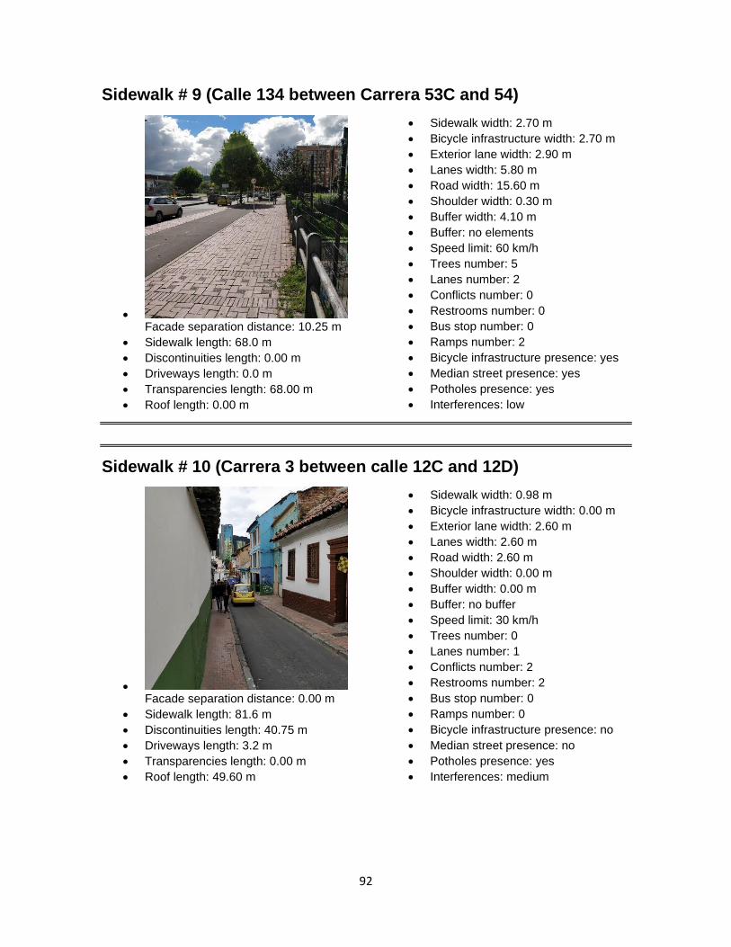
92

Sidewalk # 9 (Calle 134 between Carrera 53C and 54)














• Buffer: no elements


• Trees number: 5

• Lanes number: 2




• Ramps number: 2





Sidewalk # 10 (Carrera 3 between calle 12C and 12D)
















• Trees number: 0

• Lanes number: 1




• Ramps number: 0





93

Sidewalk # 11 (Carrera 70 between calle 74C and 73A)
















• Trees number: 0

• Lanes number: 2




• Ramps number: 0





Sidewalk # 12 (Av. Americas between Carrera 58 and 56)
















• Trees number: 5

• Lanes number: 5




• Ramps number: 2




• Interferences: no

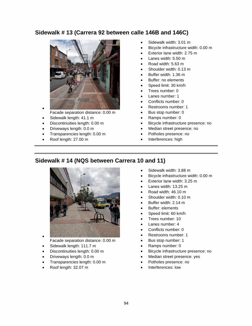
94

Sidewalk # 13 (Carrera 92 between calle 146B and 146C)
















• Trees number: 0

• Lanes number: 1




• Ramps number: 0





Sidewalk # 14 (NQS between Carrera 10 and 11)

















• Lanes number: 4




• Ramps number: 0





95

Sidewalk # 15 (Carrera 13 with calle 136)
















• Trees number: 0

• Lanes number: 2




• Ramps number: 0





Sidewalk # 16 (Av. cali between calle 131 and 130D bis)
















• Trees number: 3

• Lanes number: 3




• Ramps number: 1





96

Sidewalk # 17 (Calle 146C between Carrera 91 and 92)
















• Trees number: 0

• Lanes number: 1




• Ramps number: 0





Sidewalk # 18 (Carrera 106 between calle 131B and 132)
















• Trees number: 0

• Lanes number: 2




• Ramps number: 1





97

Sidewalk # 19 (Calle 26 south between Carrera 90A and 91C)

















• Lanes number: 2




• Ramps number: 3





Sidewalk # 20 (Carrera 4 between calle 12B and 12C)
















• Trees number: 0

• Lanes number: 1




• Ramps number: 1





98

Sidewalk # 21 (Calle 42F south between Carrera 95 and 94A)
















• Trees number: 0

• Lanes number: 2




• Ramps number: 2





Sidewalk # 22 (Carrera 71D between calle 3 south and 3)

















• Lanes number: 3




• Ramps number: 0





99

Sidewalk # 23 (Calle 150A between Carrera 103B and 104)

















• Lanes number: 2




• Ramps number: 1





Sidewalk # 24 (Aut. Sur on south transportation terminal)
















• Trees number: 0

• Lanes number: 2




• Ramps number: 0





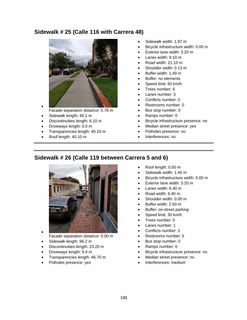
100

Sidewalk # 25 (Calle 116 with Carrera 48)
















• Trees number: 6

• Lanes number: 3




• Ramps number: 0





Sidewalk # 26 (Calle 119 between Carrera 5 and 6)
















• Trees number: 0

• Lanes number: 1




• Ramps number: 0



• Potholes presence: yes • Interferences: medium

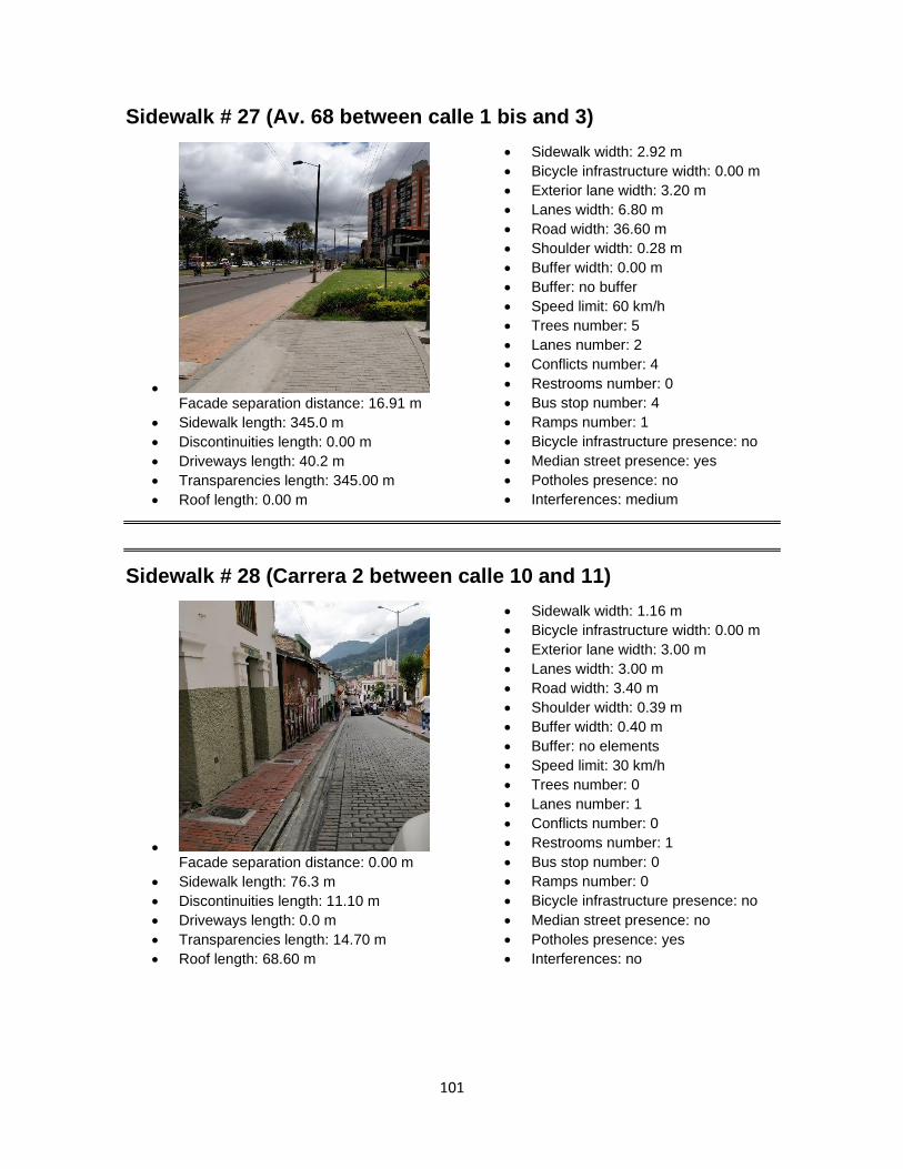
101

Sidewalk # 27 (Av. 68 between calle 1 bis and 3)
















• Trees number: 5

• Lanes number: 2




• Ramps number: 1





Sidewalk # 28 (Carrera 2 between calle 10 and 11)
















• Trees number: 0

• Lanes number: 1




• Ramps number: 0





102

Sidewalk # 29 (NQS between Carrera 19 and connector)
















• Trees number: 7

• Lanes number: 4




• Ramps number: 0





Sidewalk # 30 (Carrera 9 between calle 36 south and Carrera 11)
















• Trees number: 0

• Lanes number: 2




• Ramps number: 0



• Potholes presence: yes • Interferences: high

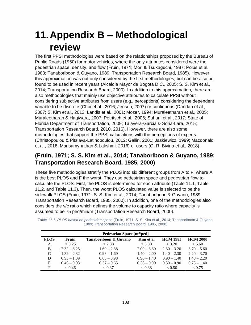
103

11. Appendix B – Methodological

review The first PPSI methodologies were based on the relationships proposed by the Bureau of

Public Roads (1950) for motor vehicles, where the only attributes considered were the

pedestrian space, density, and flow (Fruin, 1971; Mōri & Tsukaguchi, 1987; Polus et al.,

1983; Tanaboriboon & Guyano, 1989; Transportation Research Board, 1985). However,

this approximation was not only considered by the first methodologies, but can be also be

found to be used in recent years (Alcaldia Mayor de Bogota D.C., 2005; S. S. Kim et al.,

2014; Transportation Research Board, 2000). In addition to this approximation, there are

also methodologies that mainly use objective attributes to calculate PPSI without

considering subjective attributes from users (e.g., perceptions) considering the dependent

variable to be discrete (Choi et al., 2016; Jensen, 2007) or continuous (Dandan et al.,

2007; S. Kim et al., 2013; Landis et al., 2001; Mozer, 1994; Muraleetharan et al., 2005;

Muraleetharan & Hagiwara, 2007; Petritsch et al., 2006; Sahani et al., 2017; State of

Florida Department of Transportation, 2009; Talavera-Garcia & Soria-Lara, 2015;

Transportation Research Board, 2010, 2016). However, there are also some

methodologies that support the PPSI calculations with the perceptions of experts

(Christopoulou & Pitsiava-Latinopoulou, 2012; Gallin, 2001; Jaskiewicz, 1999; Macdonald

et al., 2018; Marisamynathan & Lakshmi, 2016) or users (G. R. Bivina et al., 2018).

(Fruin, 1971; S. S. Kim et al., 2014; Tanaboriboon & Guyano, 1989;

Transportation Research Board, 1985, 2000)

These five methodologies stratify the PLOS into six different groups from A to F, where A

is the best PLOS and F the worst. They use pedestrian space and pedestrian flow to

calculate the PLOS. First, the PLOS is determined for each attribute (Table 11.1, Table

11.2, and Table 11.3). Then, the worst PLOS calculated value is selected to be the

sidewalk PLOS (Fruin, 1971; S. S. Kim et al., 2014; Tanaboriboon & Guyano, 1989;

Transportation Research Board, 1985, 2000). In addition, one of the methodologies also

considers the v/c ratio which defines the volume to capacity ratio where capacity is

assumed to be 75 ped/min/m (Transportation Research Board, 2000).

Table 11.1. PLOS based on pedestrian space (Fruin, 1971; S. S. Kim et al., 2014; Tanaboriboon & Guyano, 1989; Transportation Research Board, 1985, 2000)

Pedestrian Space [m2/ped]

PLOS Fruin Tanaboriboon & Guyano Kim et al HCM 1985 HCM 2000

A > 3.25 > 2.38 > 3.30 > 3.20 > 5.60

B 2.32 – 3.25 1.60 – 2.38 2.00 – 3.30 2.30 – 3.20 3.70 – 5.60

C 1.39 – 2.32 0.98 – 1.60 1.40 – 2.00 1.40 – 2.30 2.20 – 3.70

D 0.93 – 1.39 0.65 – 0.98 0.90 – 1.40 0.90 – 1.40 1.40 – 2.20

E 0.46 – 0.93 0.37 – 0.65 0.38 – 0.90 0.50 – 0.90 0.75 – 1.40

F < 0.46 < 0.37 < 0.38 < 0.50 < 0.75

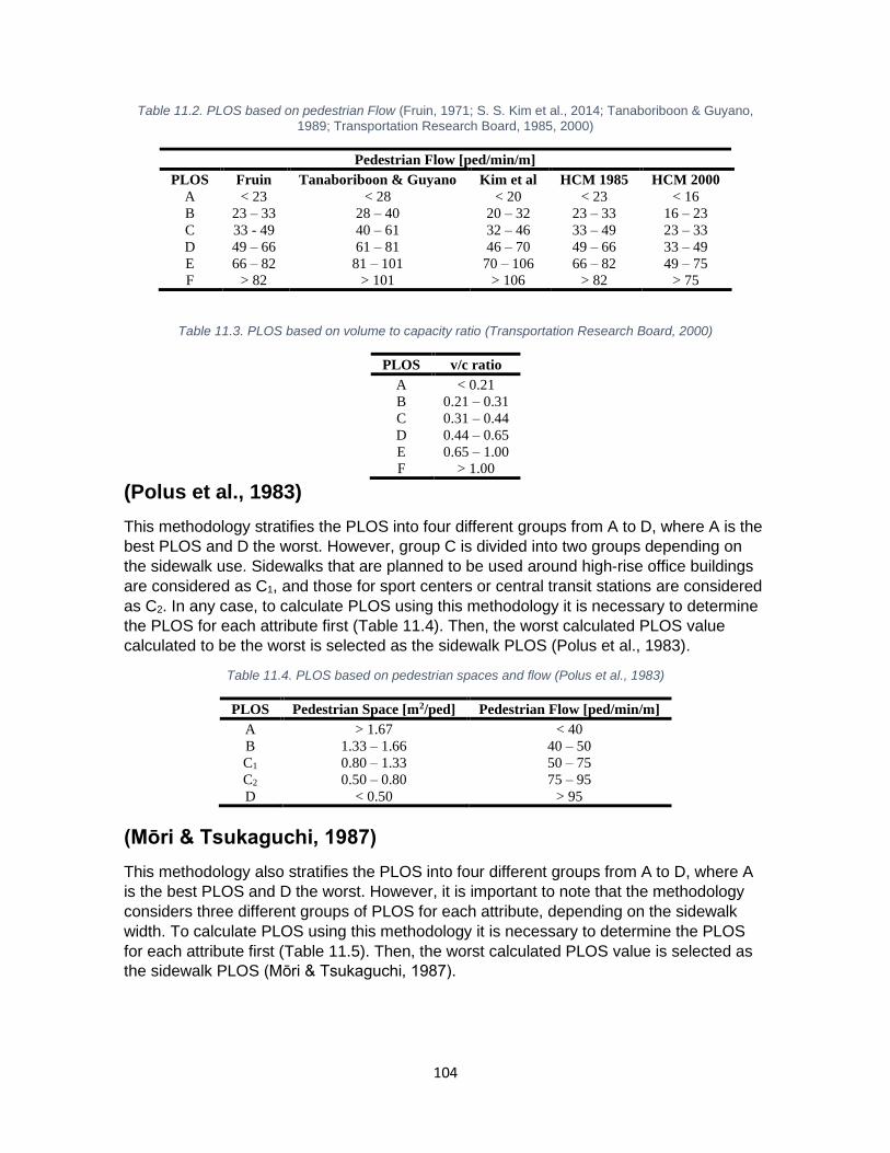
104

Table 11.2. PLOS based on pedestrian Flow (Fruin, 1971; S. S. Kim et al., 2014; Tanaboriboon & Guyano,

1989; Transportation Research Board, 1985, 2000)

Pedestrian Flow [ped/min/m]

PLOS Fruin Tanaboriboon & Guyano Kim et al HCM 1985 HCM 2000

A < 23 < 28 < 20 < 23 < 16

B 23 – 33 28 – 40 20 – 32 23 – 33 16 – 23

C 33 - 49 40 – 61 32 – 46 33 – 49 23 – 33

D 49 – 66 61 – 81 46 – 70 49 – 66 33 – 49

E 66 – 82 81 – 101 70 – 106 66 – 82 49 – 75

F > 82 > 101 > 106 > 82 > 75

Table 11.3. PLOS based on volume to capacity ratio (Transportation Research Board, 2000)

PLOS v/c ratio

A < 0.21

B 0.21 – 0.31

C 0.31 – 0.44

D 0.44 – 0.65

E 0.65 – 1.00

F > 1.00

(Polus et al., 1983)

This methodology stratifies the PLOS into four different groups from A to D, where A is the

best PLOS and D the worst. However, group C is divided into two groups depending on

the sidewalk use. Sidewalks that are planned to be used around high-rise office buildings

are considered as C1, and those for sport centers or central transit stations are considered

as C2. In any case, to calculate PLOS using this methodology it is necessary to determine

the PLOS for each attribute first (Table 11.4). Then, the worst calculated PLOS value

calculated to be the worst is selected as the sidewalk PLOS (Polus et al., 1983).

Table 11.4. PLOS based on pedestrian spaces and flow (Polus et al., 1983)

PLOS Pedestrian Space [m2/ped] Pedestrian Flow [ped/min/m]

A > 1.67 < 40

B 1.33 – 1.66 40 – 50

C1 0.80 – 1.33 50 – 75

C2 0.50 – 0.80 75 – 95

D < 0.50 > 95

(Mōri & Tsukaguchi, 1987)

This methodology also stratifies the PLOS into four different groups from A to D, where A

is the best PLOS and D the worst. However, it is important to note that the methodology

considers three different groups of PLOS for each attribute, depending on the sidewalk

width. To calculate PLOS using this methodology it is necessary to determine the PLOS

for each attribute first (Table 11.5). Then, the worst calculated PLOS value is selected as

the sidewalk PLOS (Mōri & Tsukaguchi, 1987).

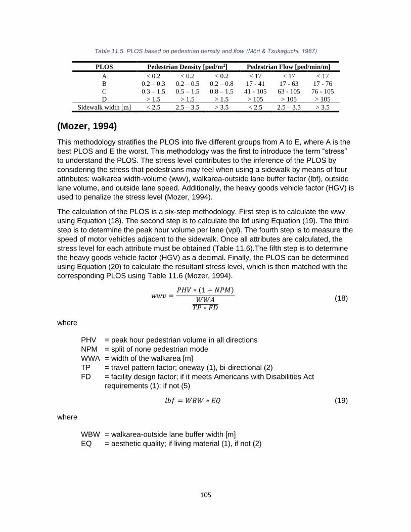
105

Table 11.5. PLOS based on pedestrian density and flow (Mōri & Tsukaguchi, 1987)

PLOS Pedestrian Density [ped/m2] Pedestrian Flow [ped/min/m]

A < 0.2 < 0.2 < 0.2 < 17 < 17 < 17

B 0.2 – 0.3 0.2 – 0.5 0.2 – 0.8 17 - 41 17 - 63 17 - 76

C 0.3 – 1.5 0.5 – 1.5 0.8 – 1.5 41 - 105 63 - 105 76 - 105

D > 1.5 > 1.5 > 1.5 > 105 > 105 > 105

Sidewalk width [m] < 2.5 2.5 – 3.5 > 3.5 < 2.5 2.5 – 3.5 > 3.5

(Mozer, 1994)

This methodology stratifies the PLOS into five different groups from A to E, where A is the

best PLOS and E the worst. This methodology was the first to introduce the term “stress”

to understand the PLOS. The stress level contributes to the inference of the PLOS by

considering the stress that pedestrians may feel when using a sidewalk by means of four

attributes: walkarea width-volume (wwv), walkarea-outside lane buffer factor (lbf), outside

lane volume, and outside lane speed. Additionally, the heavy goods vehicle factor (HGV) is

used to penalize the stress level (Mozer, 1994).

The calculation of the PLOS is a six-step methodology. First step is to calculate the wwv

using Equation (18). The second step is to calculate the lbf using Equation (19). The third

step is to determine the peak hour volume per lane (vpl). The fourth step is to measure the

speed of motor vehicles adjacent to the sidewalk. Once all attributes are calculated, the

stress level for each attribute must be obtained (Table 11.6).The fifth step is to determine

the heavy goods vehicle factor (HGV) as a decimal. Finally, the PLOS can be determined

using Equation (20) to calculate the resultant stress level, which is then matched with the

corresponding PLOS using Table 11.6 (Mozer, 1994).

𝑤𝑤𝑣 =𝑃𝐻𝑉 ∗ (1 + 𝑁𝑃𝑀)

𝑊𝑊𝐴𝑇𝑃 ∗ 𝐹𝐷

(18)

where

PHV = peak hour pedestrian volume in all directions

NPM = split of none pedestrian mode

WWA = width of the walkarea [m]

TP = travel pattern factor; oneway (1), bi-directional (2)

FD = facility design factor; if it meets Americans with Disabilities Act

requirements (1); if not (5)

𝑙𝑏𝑓 = 𝑊𝐵𝑊 ∗ 𝐸𝑄 (19)

where

WBW = walkarea-outside lane buffer width [m]

EQ = aesthetic quality; if living material (1), if not (2)

106

Table 11.6. Attribute’s stress level and PLOS (Mozer, 1994)

Stress Level wwv lbf [m] vpl [veh/h/lane] Speed [km/h] PLOS

1 100 1.7 < 50 16 A

2 200 1.3 150 32 B

3 300 1.0 300 48 C

4 400 0.6 500 64 D

5 500 0.3 > 750 80 E

𝑠𝑡𝑟𝑒𝑠𝑠 𝑙𝑒𝑣𝑒𝑙 =(2 ∗ 𝑠𝑤𝑤𝑣) + 𝑠𝑙𝑏𝑓 + 𝑠𝑣𝑝𝑙 + 𝑠𝑠𝑝𝑒𝑒𝑑

5+ 𝐻𝐺𝑉 (20)

where

wwv = stress level from walk area width-volume

lbf = stress level from walk area-outside lane buffer width

vpl = stress level from peak hour volume per lane

speed = stress level from motor vehicle speed

HGV = heavy vehicle factor as a decimal

(Christopoulou & Pitsiava-Latinopoulou, 2012; Gallin, 2001;

Jaskiewicz, 1999)

These methodologies stratify the PLOS into six different groups from A to F, where A is the

best PLOS and F the worst. These methodologies introduced the use of expert

perceptions of sidewalk attributes as a tool to determine the PLOS. To calculate the PLOS

using Jaskiewicz's (1999) methodology, it is necessary to evaluate nine different attributes

on the sidewalk (enclosure, complexity of spaces, building articulation, overhangs, path

network’s complexity, buffer, shade trees, transparencies, and physical condition) from 1

to 5 (5 = excellent, 4 = good, 3 = average, 2 = poor, 1 = very poor). Then, the scores

obtained must be aggregated and averaged to calculate the overall sidewalk evaluation

and using Table 11.7 the PLOS can be obtained. Similarly, for the methodology developed

by Gallin (2001) it is necessary to evaluate eleven different weighted attributes (access =

5, path width = 4, surface quality = 5, crossing opportunities = 4, support facilities = 2,

connectivity = 4, path environment = 2, potential for vehicle conflict = 3, path user volume

= 3, mix of path users = 4, and personal security = 4) from 0 to 4 as is outlined in Table

11.8. Then, the weight of each attribute is multiplied by the evaluation obtained from 0 to 4.

Finally, the weighted scores obtained for each attribute must be aggregated and using

Table 11.6 the PLOS can be obtained. To calculate PLOS using (Christopoulou & Pitsiava-

Latinopoulou's (2012) methodology it is necessary to evaluate eighteen different weighted

attributes (buffer width = 1.8, traffic speed = 1.2, buffer type elements = 1.5, traffic noise =

0.3, traffic volume = 0.9, discontinuities = 0.6, sidewalk width = 2.4, sidewalk width without

obstacles = 1.2, guides for the blind = 0.8, pavement condition = 2, ramps = 1.6, trees and

plants = 0.4, pedestrian volume = 1.8, safety sense = 0.3, maneuvers to avoid obstacles =

1.5, maneuvers to avoid vertical obstacles = 1.2, queue formation = 0.9, multimodal

transport presence = 0.6) from 0 to 2 as laid out in Table 11.9. Then, the weight of each

attribute is multiplied by the evaluation obtained from 0 to 2. Finally, the weighted scores

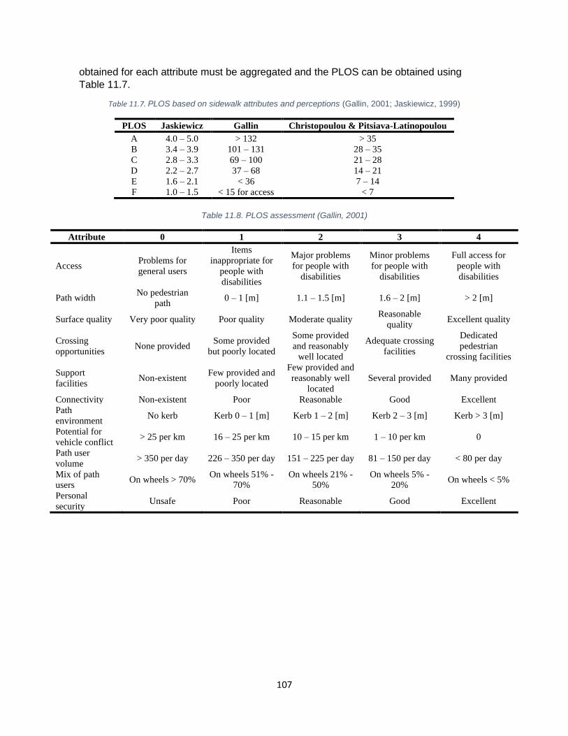
107

obtained for each attribute must be aggregated and the PLOS can be obtained using

Table 11.7.

Table 11.7. PLOS based on sidewalk attributes and perceptions (Gallin, 2001; Jaskiewicz, 1999)

PLOS Jaskiewicz Gallin Christopoulou & Pitsiava-Latinopoulou

A 4.0 – 5.0 > 132 > 35

B 3.4 – 3.9 101 – 131 28 – 35

C 2.8 – 3.3 69 – 100 21 – 28

D 2.2 – 2.7 37 – 68 14 – 21

E 1.6 – 2.1 < 36 7 – 14

F 1.0 – 1.5 < 15 for access < 7

Table 11.8. PLOS assessment (Gallin, 2001)

Attribute 0 1 2 3 4

Access Problems for

general users

Items

inappropriate for

people with

disabilities

Major problems

for people with

disabilities

Minor problems

for people with

disabilities

Full access for

people with

disabilities

Path width No pedestrian

path 0 – 1 [m] 1.1 – 1.5 [m] 1.6 – 2 [m] > 2 [m]

Surface quality Very poor quality Poor quality Moderate quality Reasonable

quality Excellent quality

Crossing

opportunities None provided

Some provided

but poorly located

Some provided

and reasonably

well located

Adequate crossing

facilities

Dedicated

pedestrian

crossing facilities

Support

facilities Non-existent

Few provided and

poorly located

Few provided and

reasonably well

located

Several provided Many provided

Connectivity Non-existent Poor Reasonable Good Excellent

Path

environment No kerb Kerb 0 – 1 [m] Kerb 1 – 2 [m] Kerb 2 – 3 [m] Kerb > 3 [m]

Potential for

vehicle conflict > 25 per km 16 – 25 per km 10 – 15 per km 1 – 10 per km 0

Path user

volume > 350 per day 226 – 350 per day 151 – 225 per day 81 – 150 per day < 80 per day

Mix of path

users On wheels > 70%

On wheels 51% -

70%

On wheels 21% -

50%

On wheels 5% -

20% On wheels < 5%

Personal

security Unsafe Poor Reasonable Good Excellent

108

Table 11.9 PLOS attribute scores for Christopoulou & Pitsiava-Latinopoulou (2012)

Attributes Score

0 1 2

Buffer width Confined to shoulder < width of an

automobile

> width of an

automobile

Traffic speed > 60 km/h 30 – 60 km/h < 30 km/h

Buffer type elements none Linear with cross Linear without crossing

opportunities

Traffic noise loud tolerable imperceptible

Traffic volume congestion Continuous flow Easy change of lane

Discontinuities > 1/100 m 1/100 m – 1/200 m < 1/200 m

Sidewalk width < 1.5 m 1.5 – 2.20 m > 2.20 m

Sidewalk width without

obstacles < 1.8 m 1.8 – 2.20 m > 2.20 m

Blind’s guides Does not exist Exists with variations

from specifications

Exists according to

specifications

Pavement condition Bad condition Medium condition Good condition

Ramps Do not exist Exists with variations

from specifications

Exists according to

specifications

Trees and plants Do not exist Existence decreasing

free width below 1.5m

Existence and does not

cause problems

Pedestrian volume heavy moderate Easy movements

Safety sense inadequate Lighting with frequent

dark spots Adequate lighting

Maneuvers to avoid

obstacles frequent moderate Rare

Maneuvers to avoid

vertical obstacles frequent moderate Rare

Queue formation frequent moderate Rare

Multimodal transport

presence

Infrastructure does not

exist Limited infrastructure Important infrastructure

(Alcaldia Mayor de Bogota D.C., 2005)

This methodology was developed to update a methodology from 1998 and was mainly

based on the 2000 version of the Highway Capacity Manual methodology. The most

relevant concepts from the Highway Capacity Manual were considered and adapted to the

city of Bogotá. This methodology stratifies the PLOS into six different groups from A to F,

where A is the best PLOS and F the worst. It uses pedestrian space, flow, and the flow-

capacity ratio, considering the capacity to be 75 ped/min/m. A two-step process calculates

the PLOS. First, the PLOS is determined for each attribute (Table 11.10). Then, the worst

calculated PLOS value is selected as the sidewalk PLOS.

109

Table 11.10. PLOS based on Alcaldia Mayor de Bogota D.C. (2005)

PLOS Space [m2/ped] Flow [ped/m/min] V/C

A > 7.00 < 14 < 0.049

B 1.00 – 7.00 15 – 91 0.050 – 0.317

C 0.77 – 0.99 92 – 115 0.318 – 0.401

D 0.40 – 0.76 116 – 194 0.402 – 0.676

E 0.17 – 0.39 195 – 287 0.677 – 1.000

F < 0.17 > 287 > 1.000

(Landis et al., 2001; Sahani et al., 2017; State of Florida

Department of Transportation, 2009)


best PLOS and F the worst. One of these methodologies was the first to propose a model

obtained from users’ perceptions but that used only sidewalk attributes to calculate the

PLOS (Landis et al., 2001). Additionally, this methodology inspired others to use the same

concept to develop a PLOS calculation model (Sahani et al., 2017; State of Florida

Department of Transportation, 2009). The calculation of PLOS using the above-mentioned

methodologies is a 2-step procedure. The first step is to calculate the model score using

Equation (21) for Landis et al. (2001), Equation (21) for State of Florida Department of

Transportation (2009), and Equations (23) to (25) for Sahani et al. (2017). Then, the PLOS

can be obtained using Table 11.11 and the previously-calculated model score.

𝑃𝐿𝑂𝑆 𝑠𝑐𝑜𝑟𝑒 = −1.2021 ln(𝑊𝑜𝑙 +𝑊𝑙 + 𝑓𝑝 ∗ %𝑂𝑆𝑃 + 𝑓𝑏 ∗ 𝑊𝑏 + 𝑓𝑠𝑤 ∗𝑊𝑠)

+ 0.253 ln (𝑉𝑜𝑙15𝐿

) + 0.0005 ∗ 𝑆𝑃𝐷2 + 5.3876 (21)

𝑃𝐿𝑂𝑆 𝑠𝑐𝑜𝑟𝑒 = −1.2276 ln(𝑊𝑜𝑙 +𝑊𝑙 + 𝑓𝑝 ∗ %𝑂𝑆𝑃 + 𝑓𝑏 ∗ 𝑊𝑏 + 𝑓𝑠𝑤 ∗𝑊𝑠)

+ 0.0091(𝑉𝑜𝑙15𝐿

)+0.004 ∗ 𝑆𝑃𝐷2 + 6.0468 (22)

where

Wol = width of outside lane [ft]

Wl = width of shoulder or bike lane [ft]

fp = on-street parking effect coefficient (0.20)

%OSP = percentage of segment with on-street parking

fb = buffer area barrier coefficient (5.37 for trees)

Wb = buffer width [ft]

fsw = sidewalk presence coefficient (6 – 0.3Ws)

Ws = sidewalk width [ft]

Vol15 = average traffic during a 15 minute period

L = total number of road lanes

SPD = motor vehicle’s average running speed [mph]

𝑃𝐿𝑂𝑆 𝑠𝑐𝑜𝑟𝑒 = 0.808 − 1.25 ln 𝐹𝑤𝑠 + 0.267 ln𝐹𝑚𝑣 + 0.0059𝐹𝑛𝑚𝑣 + 0.035𝐹𝑝𝑒𝑑+ 0.384𝑒0.401𝐹𝑜𝑏 + 0.033𝑆𝑝

(23)

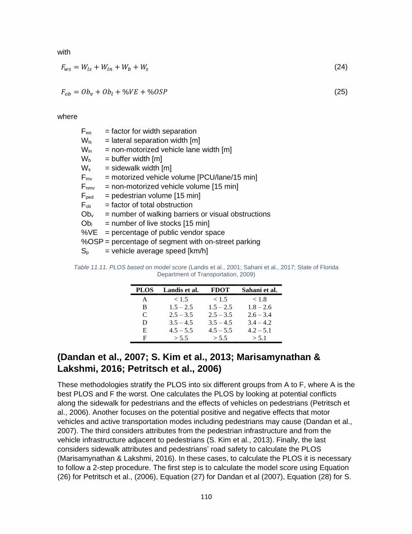
110

with

𝐹𝑤𝑠 = 𝑊𝑙𝑠 +𝑊𝑙𝑛 +𝑊𝑏 +𝑊𝑠 (24)

𝐹𝑜𝑏 = 𝑂𝑏𝑣 + 𝑂𝑏𝑙 +%𝑉𝐸 +%𝑂𝑆𝑃 (25)

where

Fws = factor for width separation

Wls = lateral separation width [m]

Wln = non-motorized vehicle lane width [m]

Wb = buffer width [m]

Ws = sidewalk width [m]

Fmv = motorized vehicle volume [PCU/lane/15 min]

Fnmv = non-motorized vehicle volume [15 min]

Fped = pedestrian volume [15 min]

Fob = factor of total obstruction

Obv = number of walking barriers or visual obstructions

Obl = number of live stocks [15 min]

%VE = percentage of public vendor space

%OSP = percentage of segment with on-street parking

Sp = vehicle average speed [km/h]

Table 11.11. PLOS based on model score (Landis et al., 2001; Sahani et al., 2017; State of Florida Department of Transportation, 2009)

PLOS Landis et al. FDOT Sahani et al.

A < 1.5 < 1.5 < 1.8

B 1.5 – 2.5 1.5 – 2.5 1.8 – 2.6

C 2.5 – 3.5 2.5 – 3.5 2.6 – 3.4

D 3.5 – 4.5 3.5 – 4.5 3.4 – 4.2

E 4.5 – 5.5 4.5 – 5.5 4.2 – 5.1

F > 5.5 > 5.5 > 5.1

(Dandan et al., 2007; S. Kim et al., 2013; Marisamynathan &

Lakshmi, 2016; Petritsch et al., 2006)


best PLOS and F the worst. One calculates the PLOS by looking at potential conflicts

along the sidewalk for pedestrians and the effects of vehicles on pedestrians (Petritsch et

al., 2006). Another focuses on the potential positive and negative effects that motor

vehicles and active transportation modes including pedestrians may cause (Dandan et al.,

2007). The third considers attributes from the pedestrian infrastructure and from the

vehicle infrastructure adjacent to pedestrians (S. Kim et al., 2013). Finally, the last

considers sidewalk attributes and pedestrians’ road safety to calculate the PLOS

(Marisamynathan & Lakshmi, 2016). In these cases, to calculate the PLOS it is necessary

to follow a 2-step procedure. The first step is to calculate the model score using Equation

(26) for Petritsch et al., (2006), Equation (27) for Dandan et al (2007), Equation (28) for S.

111

Kim et al. (2013), and Equation (29) for Marisamynathan & Lakshmi (2016). Then, the

PLOS can be obtained using Table 11.12 and the previously-calculated model score.

𝑃𝐿𝑂𝑆 𝑠𝑐𝑜𝑟𝑒 = 0.001 ∗ (𝑋𝑖𝑛𝑔 𝑤𝑖𝑑𝑡ℎ

𝑚𝑖𝑙𝑒) + 0.008 ∗ (𝑉𝑜𝑙15) + 1.43 (26)

where

Xing width/mile = total width of crossings at conflict locations per mile [ft]

Vol15 = average 15-min volume on adjacent roadway

𝑃𝐿𝑂𝑆 𝑠𝑐𝑜𝑟𝑒 = −1.43 + 0.006𝑄𝐵 − 0.003𝑄𝑃 + 0.056(𝑄𝑉𝑊𝑟) + 11.24(𝑃 − 1.17𝑃3) (27)

where

QB = bicycle traffic during a five-minute period

QP = pedestrian traffic during a five-minute period

QV = vehicle traffic during a five-minute period [pcu]

P = driveway access quantity per meter

Wr = distance between sidewalk and vehicle lane [m]

𝑃𝑆 = 2.485 + 3.001 ln𝑊𝑡 − 1.438 ln𝑊𝑏 − 0.544 ln𝑊𝑠 + 0.045𝑆𝑃𝐷 + 0.017𝑉𝑂𝐿5 (28)

where

PS = LOS perceived by pedestrians

Wt = traffic lane width [m]

Wb = buffer width [m]

Ws = sidewalk width [m]

SPD = vehicle speed [km/h]

VOL5 = vehicle volume [5 min]

𝑃𝐿𝑂𝑆 = 3.404 ln(𝑆𝑆𝐶 + 𝐺𝑠𝑤 + 𝐵𝑠𝑤) + 15.215 ln(𝑉𝑜𝑙15) − 17.639 ln(𝑊𝑠𝑤) − 20.770 (29)

where

SSC = sidewalk surface condition (1: very good, 2: good, 3: average, 4: poor, 5:

very poor)

Gsw = guard rail presence (0: absence, 1: presence)

Bsw = barrier presence (0: absence, 1: presence of trees/pole/boxes/drainage, 2:

combination)

Vol15 = traffic volume [15 min]

Wsw = sidewalk width [m]

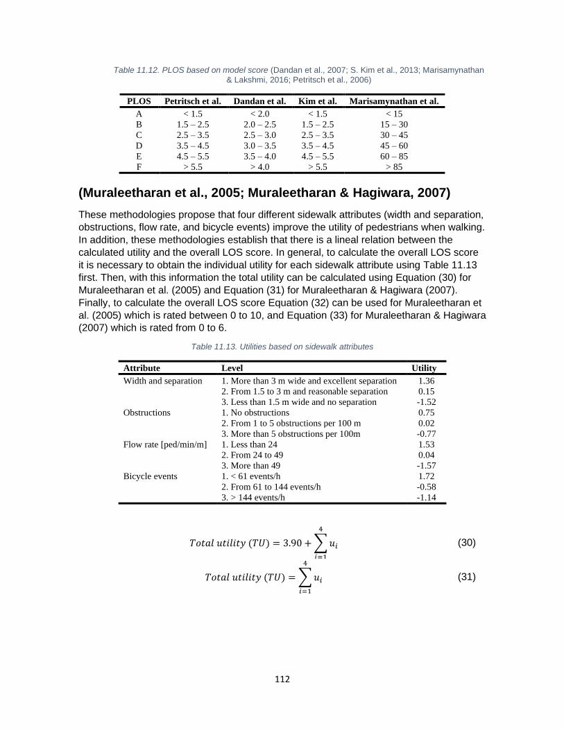
112

Table 11.12. PLOS based on model score (Dandan et al., 2007; S. Kim et al., 2013; Marisamynathan

& Lakshmi, 2016; Petritsch et al., 2006)

PLOS Petritsch et al. Dandan et al. Kim et al. Marisamynathan et al.

A < 1.5 < 2.0 < 1.5 < 15

B 1.5 – 2.5 2.0 – 2.5 1.5 – 2.5 15 – 30

C 2.5 – 3.5 2.5 – 3.0 2.5 – 3.5 30 – 45

D 3.5 – 4.5 3.0 – 3.5 3.5 – 4.5 45 – 60

E 4.5 – 5.5 3.5 – 4.0 4.5 – 5.5 60 – 85

F > 5.5 > 4.0 > 5.5 > 85

(Muraleetharan et al., 2005; Muraleetharan & Hagiwara, 2007)

These methodologies propose that four different sidewalk attributes (width and separation,

obstructions, flow rate, and bicycle events) improve the utility of pedestrians when walking.

In addition, these methodologies establish that there is a lineal relation between the

calculated utility and the overall LOS score. In general, to calculate the overall LOS score

it is necessary to obtain the individual utility for each sidewalk attribute using Table 11.13

first. Then, with this information the total utility can be calculated using Equation (30) for

Muraleetharan et al. (2005) and Equation (31) for Muraleetharan & Hagiwara (2007).

Finally, to calculate the overall LOS score Equation (32) can be used for Muraleetharan et

al. (2005) which is rated between 0 to 10, and Equation (33) for Muraleetharan & Hagiwara

(2007) which is rated from 0 to 6.

Table 11.13. Utilities based on sidewalk attributes

Attribute Level Utility

Width and separation 1. More than 3 m wide and excellent separation 1.36

2. From 1.5 to 3 m and reasonable separation 0.15

3. Less than 1.5 m wide and no separation -1.52

Obstructions 1. No obstructions 0.75

2. From 1 to 5 obstructions per 100 m 0.02

3. More than 5 obstructions per 100m -0.77

Flow rate [ped/min/m] 1. Less than 24 1.53

2. From 24 to 49 0.04

3. More than 49 -1.57

Bicycle events 1. < 61 events/h 1.72

2. From 61 to 144 events/h -0.58

3. > 144 events/h -1.14

𝑇𝑜𝑡𝑎𝑙 𝑢𝑡𝑖𝑙𝑖𝑡𝑦 (𝑇𝑈) = 3.90 +∑𝑢𝑖

4

𝑖=1

(30)

𝑇𝑜𝑡𝑎𝑙 𝑢𝑡𝑖𝑙𝑖𝑡𝑦 (𝑇𝑈) =∑𝑢𝑖

4

𝑖=1

(31)

113

𝑂𝑣𝑒𝑟𝑎𝑙𝑙 𝐿𝑂𝑆 𝑠𝑐𝑜𝑟𝑒 =

{

𝑇𝑈 < 3.53 5 ∗ (

𝑇𝑈 + 1.1

4.63)

𝑇𝑈 > 3.53 5 + (5 ∗ (𝑇𝑈 − 3.53

5.73))

(32)

𝑂𝑣𝑒𝑟𝑎𝑙𝑙 𝐿𝑂𝑆 𝑠𝑐𝑜𝑟𝑒 = 6 ∗ (𝑇𝑈 + 5

10.36) (33)

(Choi et al., 2016; Jensen, 2007)

These methodologies proposed a discrete Likert scale for satisfaction to predict PLOS.

Jensen (2007) was one of the first authors to propose a discrete scale with six different

categories (very satisfied (VS), moderately satisfied (MS), a little satisfied (LS), a little

dissatisfied (LD), moderately dissatisfied (MD), and very dissatisfied (VD)) to calculate

PLOS. Almost ten years later, Choi et al. (2016) also propose a discrete scale to predict

PLOS using satisfaction, but only considering three different categories (satisfied, average,

and unsatisfied). A logit model was proposed to predict the PLOS in both cases where a

utility is calculated to predict the probability to be selected for each of the satisfaction

categories considering some attributes of the sidewalk.

Jensen (2007) states that to calculate the PLOS it is necessary to obtain the cumulative

utility for each category considering some sidewalk attributes using Equation (34). To use

Equation (34), the discrete attribute parameters can be obtained using Table 11.14. Once

the utility cumulative is calculated, the probability for each satisfaction category can be

obtained using Equations (35) to (40). The satisfaction category with the highest

probability will be selected as the PLOS for the sidewalk.

𝑙𝑜𝑔𝑖𝑡(𝑝) = 𝛼 +𝑊𝐴 + 𝐴𝑅𝐸𝐴 − 0.002476 ∗ 𝑀𝑂𝑇 + 0.0000003364 ∗ 𝑀𝑂𝑇2

− 0.0303 ∗ 𝑆𝑃𝐸𝐸𝐷 + 0.00002211 ∗ 𝑆𝑃𝐸𝐸𝐷 ∗𝑀𝑂𝑇 − 0.005432∗ 𝑃𝐸𝐷 + 0.000005062 ∗ 𝑃𝐸𝐷2 − 0.003772 ∗ 𝐵𝐼𝐾𝐸 + 0.000003111∗ 𝐵𝐼𝐾𝐸2 + 0.4408 ∗ 𝐵𝑈𝐹 − 0.0365 ∗ 𝐵𝑈𝐹2 − 0.05286 ∗ 𝑃𝐴𝑅𝐾+ 1.0180 ∗ 𝑀𝐸𝐷 + 0.2938 ∗ 𝑆𝐵 + 0.6277 ∗ 𝐵𝐿 + 0.7380 ∗ 𝐿𝐴𝑁𝐸+ 0.3311 ∗ 𝑇𝑅𝐸𝐸

(34)

where

logit(p) = utility function cumulative logit model

α = parameter of the response level of satisfaction (Table 11.14)

WA = type of walking area (Table 11.14)

AREA = type of roadside development or landscape (Table 11.14)

MOT = motor vehicles per hour

SPEED = average motor vehicle speed [km/h]

PED = number of pedestrians per hour

BIKE = number of bicycles and mopeds per hour

BUF = width of buffer area [m]

PARK = parked motor vehicle on road per 100 m

MED = 1 if median present, 0 otherwise

SB = sidewalk width [m]

BL = sidewalk and nearest drive lane width [m]

114

LANE = 1 if there are four or more drive lanes, 0 otherwise

TREE = 1 if there is one tree or more per 50 m, 0 otherwise

Table 11.14. Discrete attribute parameters (Jensen, 2007)

α WA AREA

Very satisfied -2.8526 Sidewalk concrete 3.5486 Residential 0.4871

Moderately satisfied -1.2477 Sidewalk asphalt 1.9149 Shopping 0.5385

A little satisfied -0.0646 Bicycle track 1.0124 Mixed -1.6349

A little dissatisfied 0.8758 Bike lane -2.8293 Rural fields 1.2380

Moderately dissatisfied 2.2543 Driving lane -3.6464 Rural forest 0.5122

𝑉𝑆 = 1 −1

1 + exp(𝑙𝑜𝑔𝑖𝑡(𝑝)𝑉𝑆) (35)

𝑀𝑆 = 1 − 𝑉𝑆 −1

1 + exp(𝑙𝑜𝑔𝑖𝑡(𝑝)𝑀𝑆) (36)

𝐿𝑆 = 1 − 𝑉𝑆 −𝑀𝑆 −1

1 + exp(𝑙𝑜𝑔𝑖𝑡(𝑝)𝐿𝑆) (37)

𝐿𝐷 = 1 − 𝑉𝑆 −𝑀𝑆 − 𝐿𝑆 −1

1 + exp(𝑙𝑜𝑔𝑖𝑡(𝑝)𝐿𝐷) (38)

𝑀𝐷 = 1 − 𝑉𝑆 −𝑀𝑆 − 𝐿𝑆 − 𝐿𝐷 −1

1 + exp(𝑙𝑜𝑔𝑖𝑡(𝑝)𝑀𝐷) (39)

𝑉𝐷 = 1 − 𝑉𝑆 −𝑀𝑆 − 𝐿𝑆 − 𝐿𝐷 −𝑀𝐷 (40)

Similarly, for the methodology proposed by Choi et al. (2016) it is necessary to obtain the

cumulative utility for each category including some sidewalk attributes using Equation (41).

Once the utility cumulative is calculated, the probability for each satisfaction category can

be obtained using Equations (42) to (44). The satisfaction category with the highest

probability is selected as the PLOS for the sidewalk.

𝑙𝑜𝑔𝑖𝑡(𝑝) = 𝛽 − 0.216𝑋1 − 0.093𝑋2 − 0.260𝑋3 + 0.027𝑋4 + 0.061𝑋5 − 0.293𝑋6− 0.332𝑋7 − 0.137𝑋8 + 0.317𝑋9 + 0.060𝑋10

(41)

where

logit(p) = utility function cumulative logit model

β = satisfaction parameter (satisfied = -0.574, average = 3.184)

X1 = pedestrian volume per day

X2 = crosswalk presence (1 = yes, 0 = no)

X3 = number of lanes per direction

X4 = median presence (1 = yes, 0 = no)

X5 = bike lane presence (1 = yes, 0 = no)

X6 = driveway presence (1 = yes, 0 = no)

X7 = planting strip presence (1 = yes, 0 = no)

X8 = bus stop presence (1 = yes, 0 = no)

X9 = commercial land use (1 = yes, 0 = no)

X10 = business land use (1 = yes, 0 = no)

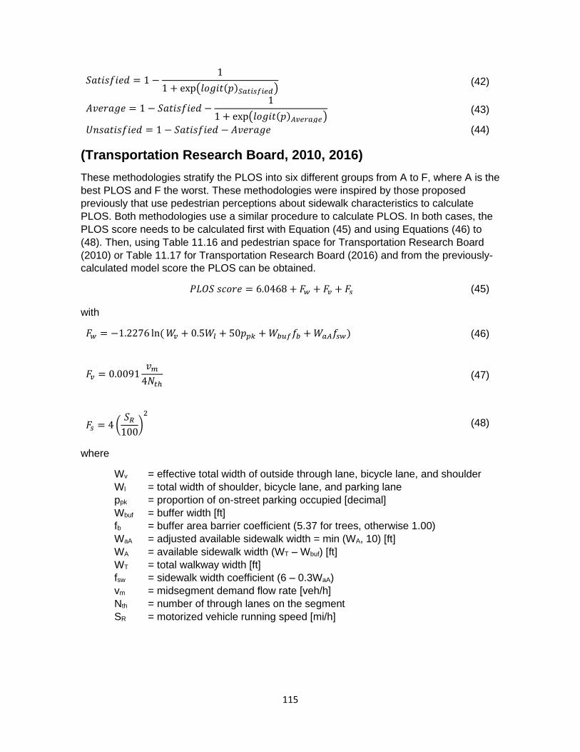
115

𝑆𝑎𝑡𝑖𝑠𝑓𝑖𝑒𝑑 = 1 −1

1 + exp(𝑙𝑜𝑔𝑖𝑡(𝑝)𝑆𝑎𝑡𝑖𝑠𝑓𝑖𝑒𝑑) (42)

𝐴𝑣𝑒𝑟𝑎𝑔𝑒 = 1 − 𝑆𝑎𝑡𝑖𝑠𝑓𝑖𝑒𝑑 −1

1 + exp(𝑙𝑜𝑔𝑖𝑡(𝑝)𝐴𝑣𝑒𝑟𝑎𝑔𝑒) (43)

𝑈𝑛𝑠𝑎𝑡𝑖𝑠𝑓𝑖𝑒𝑑 = 1 − 𝑆𝑎𝑡𝑖𝑠𝑓𝑖𝑒𝑑 − 𝐴𝑣𝑒𝑟𝑎𝑔𝑒 (44)

(Transportation Research Board, 2010, 2016)


best PLOS and F the worst. These methodologies were inspired by those proposed

previously that use pedestrian perceptions about sidewalk characteristics to calculate

PLOS. Both methodologies use a similar procedure to calculate PLOS. In both cases, the

PLOS score needs to be calculated first with Equation (45) and using Equations (46) to

(48). Then, using Table 11.16 and pedestrian space for Transportation Research Board

(2010) or Table 11.17 for Transportation Research Board (2016) and from the previously-

calculated model score the PLOS can be obtained.

𝑃𝐿𝑂𝑆 𝑠𝑐𝑜𝑟𝑒 = 6.0468 + 𝐹𝑤 + 𝐹𝑣 + 𝐹𝑠 (45)

with

𝐹𝑤 = −1.2276 ln(𝑊𝑣 + 0.5𝑊𝑙 + 50𝑝𝑝𝑘 +𝑊𝑏𝑢𝑓𝑓𝑏 +𝑊𝑎𝐴𝑓𝑠𝑤) (46)

𝐹𝑣 = 0.0091𝑣𝑚4𝑁𝑡ℎ

(47)

𝐹𝑠 = 4(𝑆𝑅100

)2

(48)

where

Wv = effective total width of outside through lane, bicycle lane, and shoulder

Wl = total width of shoulder, bicycle lane, and parking lane

ppk = proportion of on-street parking occupied [decimal]

Wbuf = buffer width [ft]

fb = buffer area barrier coefficient (5.37 for trees, otherwise 1.00)

WaA = adjusted available sidewalk width = min (WA, 10) [ft]

WA = available sidewalk width (WT – Wbuf) [ft]

WT = total walkway width [ft]

fsw = sidewalk width coefficient (6 – 0.3WaA)

vm = midsegment demand flow rate [veh/h]

Nth = number of through lanes on the segment

SR = motorized vehicle running speed [mi/h]

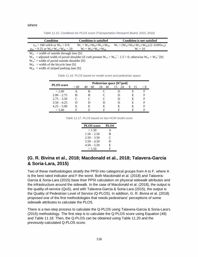
116

where

Table 11.15. Conditions for PLOS score (Transportation Research Board, 2010, 2016)

Condition Condition is satisfied Condition is not satisfied

vm > 160 veh/h or WA > 0 ft Wv = Wol+Wbl+Wos+Wpk Wv = (Wol+Wbl+Wos+Wpk) (2–0.005vm)

ppk > 0.25 or Wbl+Wos+Wpk < 10 Wl = Wbl+Wos+Wpk Wl = 10

Wol = width of outside through lane [ft]

Wos = adjusted width of paved shoulder (if curb present Wos = Wos* - 1.5 > 0, otherwise Wos = Wos

* [ft]

Wos* = width of paved outside shoulder [ft]

Wbl = width of the bicycle lane [ft]

Wpk = width of striped parking lane [ft]

Table 11.16. PLOS based on model score and pedestrian space

PLOS score Pedestrian space [ft2/ped]

> 60 40 – 60 24 – 40 15 – 24 8 – 15 < 8

< 2.00 A B C D E F

2.00 – 2.75 B B C D E F

2.75 – 3.50 C C C D E F

3.50 – 4.25 D D D D E F

4.25 – 5.00 E E E E E F

> 5.00 F F F F F F

Table 11.17. PLOS based on last HCM model score

PLOS score PLOS

< 1.50 A

1.50 – 2.50 B

2.50 – 3.50 C

3.50 – 4.50 D

4.50 – 5.50 E

> 5.50 F

(G. R. Bivina et al., 2018; Macdonald et al., 2018; Talavera-Garcia

& Soria-Lara, 2015)

Two of these methodologies stratify the PPSI into categorical groups from A to F, where A

is the best rated indicator and F the worst. Both Macdonald et al. (2018) and Talavera-

Garcia & Soria-Lara (2015) base their PPSI calculation on physical sidewalk attributes and

the infrastructure around the sidewalk. In the case of Macdonald et al. (2018), the output is

the quality-of-service (QoS), and with Talavera-Garcia & Soria-Lara (2015), the output is

the Quality of Pedestrian Level of Service (Q-PLOS). In addition, G. R. Bivina et al. (2018)

proposed one of the first methodologies that needs pedestrians’ perceptions of some

sidewalk attributes to calculate the PLOS.

There is a two-step process to calculate the Q-PLOS using Talavera-Garcia & Soria-Lara's

(2015) methodology. The first step is to calculate the Q-PLOS score using Equation (49)

and Table 11.18. Then, the Q-PLOS can be obtained using Table 11.20 and the

previously-calculated Q-PLOS score.

117

𝑄𝑃𝐿𝑂𝑆 =0.76 ∗ 𝐶 + 0.95 ∗ 𝑊 + 0.91 ∗ 𝑆 + 0.98 ∗ 𝑇𝐷 + 0.87 ∗ 𝐶𝐷

4.47 (49)

where

Table 11.18. Sidewalk attribute parameters (Talavera-Garcia & Soria-Lara, 2015)

QL Connectivity (C) Width [m] (W) Speed [km/h]

and lanes (S)

Trees density

[tree/km2] (TD)

Commercial density

[shops/km2] (CD)

1

According to city’s

values

> 3 > 20000

According to city’s

values

2 2.25 – 3 20 – 30 15000 – 20000

3 1.5 – 2.25 50 (1 lane) 10000 – 15000

4 0.9 – 1.5 50 (2 lanes) 5000 – 10000

5 < 0.9 50 (3 lanes) < 5000

Similarly, a two-step process is necessary for that proposed by G. R. Bivina et al. (2018).

The first step is to calculate the PLOS score using Equation (50) and Table 11.19. Then,

the PLOS can be obtained by using Table 11.20 and the previously-calculated PLOS

score.

𝑃𝐿𝑂𝑆 =∑𝐴𝑖 ∗ 𝐵𝑖

10

𝑖=1

(50)

where

Ai = relative importance weight of each sidewalk characteristic ()

Bi = Perceived satisfaction score for each sidewalk characteristic (from 1 to 5)

Table 11.19. Sidewalk characteristics’ weights per land use (G. R. Bivina et al., 2018)

Sidewalk

characteristics

Land Uses

Residential Commercial Institutional Terminal Recreational

Surface 3.14 3.17 3.35 2.36 2.40

Width 2.63 3.53 3.28 1.98 3.04

Obstructions 2.39 3.30 3.47 1.77 3.31

Vehicle conflict 2.71 3.04 3.51 2.15 3.30

Continuity 2.22 2.51 2.71 1.71 2.90

Encroachment 2.46 3.08 3.08 1.55 2.71

Crossing facilities 2.71 3.23 3.35 1.97 3.33

Security 2.31 2.72 2.98 1.94 2.78

Comfort 1.96 2.87 2.34 1.52 3.34

Environment 2.20 2.97 3.09 1.67 2.92

Finally, for the methodology proposed by Macdonald et al. (2018), a four-step process is

applied. The first step is to calculate the block segment score according to eight different

sidewalk characteristics. When each core complies with the sidewalk infrastructure, one

point is added to the score. A maximum of eight points can be obtained from this step.

- Core 1: Sidewalk width (+1 if accomplish at least one)

o Arterial street, 4 lanes or fewer: 12 feet

118

o Arterial street, 5 lanes or more: 15 feet

o Urban core commercial street, 4 lanes, up to 10 story buildings: 12 feet

o Urban core commercial street, 4 lanes, 10 + story buildings: 15 feet

o Collector street, 2 lanes: 8 feet

o Neighborhood commercial, 2 lanes: 10 feet

- Core 2: Lanes and speed (+1 if accomplish)

o Five or fewer traffic lanes

o Vehicle speeds no more than 35 mph

- Core 3: Buffer (+1 if accomplish at least three)

o On-street parking

o Delineated bike lane

o Planting strip with kerb present

o Line of street trees planted no more than 30 ft apart

o Line of permanent street furniture

- Core 4: Trees (+1 if accomplish)

o Tree canopy presence

- Core 5: Visual (+1 if accomplish at least three)

o Transparent building materials

o Varying storefronts or facades

o Activated sidewalk elements presence

o Adjacent open spaces

o Public art

o Buildings of architectural interest

- Core 6: Enclosure (+1 if accomplish at least one)

o Streets wider than two lanes, building height at least half the ROW width

o Streets up to two lanes, building of any height

o If there are open spaces, presence of features giving a sense of enclosure

- Core 7: Protected crossing (+1 if accomplish at least two)

o Painted crosswalk

o Pedestrian walk signals

o Medians presence

o Stop signs

o Traffic circles

- Core 8: Accessibility (+1 if accomplish at least three)

o Kerb ramps

o Tactile warning strips

o Audible walk signals

o Level pavement

The second step is to bonify the block segment according to ten different assets that may

be found on the sidewalk, that generate a positive effect on pedestrians (Macdonald et al.,

2018). For each asset observed on the sidewalk, 0.5 is added to the segment’s score. A

maximum of five points can be obtained from this step.

- Attractive views of hills, mountains, water, major buildings, urban skylines or other

natural or architectural landmark

- High-quality signage or other wayfinding aids such as maps and kiosks

- Connection to off-street multi-use pathways or regional trail network

119

- Location within a cultural or historic district, safe-routes-to-school route or other

pedestrian-friendly designation

- Presence of high-quality landscape architecture within or adjacent to the right-of-

way, including storm water management features

- Presence of raised crosswalks, special pavements, pedestrian scrambles or other

pedestrian-friendly intersection treatments at either end of block segment

- Location on a direct path to nearby transit stop or major civic destination such as

school, museum, stadium or concert hall

- Design mitigation to address adverse environmental conditions, such as excessive

wind, rain, and sun exposure

- Extra traffic calming devices, such as chicanes or speed bumps

- On boulevards, walking paths along the medians

The third step is to detract points from the block segment according to nine different

characteristics that potentially generate nuisances for pedestrians (Macdonald et al.,

2018). For each of these features observed on the sidewalk, 0.5 is added to the segment’s

demerits. A maximum of 4.5 points can be obtained in this step.

- Inadequate municipal services and maintenance (at least two)

o Lack of streetlights for the whole block length

o Lack of at least one trash/recycling receptacle on each side of the street

o Non-level, broken or poorly maintained pavement

o Excessive graffiti, broken windows or other evidence of vandalism

o Poor drainage or localized flooding

- Excessive street-level building vacancies (three or more)

- Excessively steep grade

- Poorly controlled interactions between pedestrians, bicycles, and skateboards

- Excessive noise from at least one permanent source

- Excessive visual clutter from overhead utility lines or other permanent features

- Three or more driveways

- Presence of major barriers to pedestrians

- Very poor or no design mitigations to address adverse environmental conditions

Finally, last step is to calculate the resulting final score using Equation (51) and the PLOS

using Table 11.20.

𝐹𝑖𝑛𝑎𝑙 𝑠𝑐𝑜𝑟𝑒 = 𝑏𝑙𝑜𝑐𝑘 𝑠𝑒𝑔𝑚𝑒𝑛𝑡 𝑠𝑐𝑜𝑟𝑒 + 𝑏𝑜𝑛𝑢𝑠 − 𝑑𝑒𝑚𝑒𝑟𝑖𝑡𝑠 (51)

Table 11.20. PLOS thresholds (G. R. Bivina et al., 2018; Macdonald et al., 2018; Talavera-Garcia & Soria-Lara, 2015)

PLOS/Q-PLOS/SQ Talavera-Garcia & Soria-Lara Macdonald et al Bivina et al

A < 1.5 > 6.0 > 125

B 1.5 – 2.5 5.0 or 5.5 100 – 125

C 2.5 – 3.5 4.0 or 4.5 75 – 100

D 3.5 – 4.5 3.0 or 3.5 49 – 75

E > 4.5 25 – 50

F < 3.0 > 25

The role of perceptions in pedestrian quality of service

Documents