The role of multi-method linear solvers in PDE-based simulations

The Role of Multi-Method Linear Solvers in

PDE-Based Simulations?

S. Bhowmick1, L. McInnes2, B. Norris2, and P. Raghavan1

1 Department of Computer Science and Engineering, The Pennsylvania StateUniversity, 220 Pond Lab, University Park, PA 16802-6106. E-mail

fbhowmick,[email protected] Mathematics and Computer Sciences Division, Argonne National Laboratory, 9700South Cass Ave., Argonne IL 60439-4844. E-mail fmcinnes,[email protected].

Abstract. The solution of large-scale, nonlinear PDE-based simulationstypically depends on the performance of sparse linear solvers, which maybe invoked at each nonlinear iteration. We present a framework for us-ing multi-method solvers in such simulations to potentially improve theexecution time and reliability of linear system solution. We consider com-

posite solvers, which provide reliable linear solution by using a sequenceof preconditioned iterative methods on a given system until convergenceis achieved. We also consider adaptive solvers, where the solution methodis selected dynamically to match the attributes of linear systems as theychange during the course of the nonlinear iterations. We demonstrate howsuch multi-method composite and adaptive solvers can be developed us-ing advanced software architectures such as PETSc, and we report ontheir performance in a computational uid dynamics application.

1 Introduction

Many areas of computational modeling, for example, turbulent uid ow, astro-physics, and fusion, require the numerical solution of nonlinear partial di�eren-tial equations with di�erent spatial and temporal scales [13, 18]. The governingequations are typically discretized to produce a nonlinear system of the formf(u) = 0, where f : Rn ! Rn. When such systems are solved using semi-implicit or implicit methods, the computationally intensive part often involvesthe solution of large, sparse linear systems.

A variety of competing algorithms are available for sparse linear solution, in-cluding both direct and iterative methods. Direct methods rely on sparse matrixfactorization and will successfully compute the solution if one exists. However,sparse factorization causes zeroes in the coe�cient matrix to become nonzeroes

? This work was supported in part by the Maria Goeppert Mayer Award from theU. S. Department of Energy and Argonne National Laboratory, by the Mathemat-ical, Information, and Computational Sciences Division subprogram of the O�ceof Computational Technology Research, U. S. Department of Energy under Con-tract W-31-109-Eng-38, and by the National Science Foundation through grantsACI-0102537, DMR-0205232, and ECS-0102345.

2

in the factor, thus increasing memory demands. Hence, the method could failfor lack of memory. Additionally, even when su�cient memory is available, thecomputational cost might be quite high, especially when the sparse coe�cientmatrix changes at each nonlinear iteration and must therefore be refactored.Krylov subspace iterative methods require little additional memory, but theyare not robust; convergence can be slow or fail altogether. Various precondi-tioners can be combined with Krylov methods to produce solvers with vastlydi�ering computational costs and convergence behaviors. It is typically neitherpossible nor practical to predict a priori which sparse linear solver algorithmworks best for a given class of problems. Furthermore, the numerical propertiesof the linear systems can change during the course of the nonlinear iterations.Consequently, the most e�ective linear solution method need not be the sameat di�erent stages of the simulation. This situation has motivated us (and otherresearchers) to explore the potential bene�ts of multi-method solver schemes forimproving the performance of PDE-based simulations [5, 8, 11].

Ern et al have investigated the performance of several preconditioned Kryloviterations and stationary methods in nonlinear elliptic PDEs [11]; their workis towards a polyalgorithmic approach. Polyalgorithms have been studied formultiprocessor implementations by Barrett et al in a formulation where di�er-ent types of Krylov methods are applied in parallel to the same problem [5].Our work on multi-method solvers for PDE-based applications focuses on for-mulating general-purpose metrics that can be used in di�erent ways to increasereliability and reduce execution times. We also consider the instantiation of suchmulti-method schemes using advanced object-oriented software systems, such asPETSc [3, 4], with well-de�ned abstract interfaces and dynamic method selec-tion.

The �rst type of multi-method solver we consider is a composite, which com-prises several underlying (base) methods; each base method is applied in turn tothe same linear system until convergence is achieved. A composite solver couldfail in the event that all underlying methods fail on the problem, but in prac-tice this is rare even with as few as three or four methods. The composite isthus more reliable than any of its constituent methods. However, the order inwhich base methods are applied can signi�cantly a�ect total execution time. Wehave developed a combinatorial scheme for constructing an optimal compositein terms of simple observable metrics such as execution time and mean failurerates [6, 7]. The second type of multi-method scheme is an adaptive solver; sucha solver once again comprises several base methods, but only one base methodis applied to a given linear system. The numerical properties of the linear sys-tems can change during the course of nonlinear iterations [15], and our adaptivesolver attempts to select a base method for each linear system that best matchesits numerical attributes. Once again, our focus is on automated method selec-tion using metrics such as normalized time per iteration and both linear andnonlinear convergence rates.

In this paper, we provide overviews of our composite and adaptive solvertechniques and demonstrate their e�ectiveness in a computational uid dynam-

3

ics application. In Section 2, we describe a PDE-based simulation of driven cavity ow and our solution approach using inexact Newton methods. In Section 3 weillustrate how an optimal composite solver can be constructed using a combi-natorial scheme to yield ideal reliability for linear solution and an overall fastersimulation. In Section 4, we describe our method for constructing an adaptivesolver and report on observed reductions in simulation times. Section 5 containsconcluding remarks.

2 Problem Description and Solution Methods

We consider a driven cavity ow simulation to illustrate the bene�ts of multi-method solvers in the context of nonlinear PDEs. This simulation incorporatesnumerical features that are common in many large-scale scienti�c applications,yet is su�ciently simple to enable succinct description. We introduce the modelproblem in Section 2.1 and discuss our solution schemes using inexact Newtonmethods in Section 2.2.

2.1 Simulation of Driven Cavity Flow

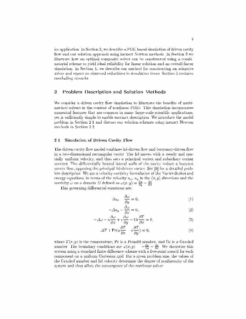
The driven cavity ow model combines lid-driven ow and buoyancy-driven owin a two-dimensional rectangular cavity. The lid moves with a steady and spa-tially uniform velocity, and thus sets a principal vortex and subsidiary cornervortices. The di�erentially heated lateral walls of the cavity induce a buoyantvortex ow, opposing the principal lid-driven vortex. See [9] for a detailed prob-lem description. We use a velocity-vorticity formulation of the Navier-Stokes andenergy equations, in terms of the velocity ux, uy in the (x; y) directions and thevorticity ! on a domain de�ned as !(x; y) = @u

@y+ @v

@x.

This governing di�erential equations are:

��ux +@!

@y= 0; (1)

��uy +@!

@x= 0; (2)

��! + u@!

@x+ v

@!

@y�Gr

@T

@x= 0; (3)

��T + Pr(u@T

@x+ v

@T

@y) = 0; (4)

where T (x; y) is the temperature, Pr is a Prandtl number, and Gr is a Grashofnumber. The boundary conditions are !(x; y) = �@u

@y+ @v

@x. We discretize this

system using a standard �nite di�erence scheme with a �ve-point stencil for eachcomponent on a uniform Cartesian grid. For a given problem size, the values ofthe Grashof number and lid velocity determine the degree of nonlinearity of thesystem and thus a�ect the convergence of the nonlinear solver.

4

2.2 Inexact Newton Methods

We use inexact Newton methods (see, e.g., [16]) to simultaneously solve theequations (1) through (4), which have the combined form

f(u) = 0: (5)

We use a Krylov iterative method to (approximately) solve the Newton correc-tion equation

f 0(u`�1) �u` = �f(u`�1); (6)

in the sense that the linear residual norm jjf 0(u`�1) �u`+f(u`�1)jj is su�cientlysmall. We then update the iterate via u` = u`�1 + � � �u`; where � is a scalardetermined by a line search technique such that 0 < � � 1. We terminate theNewton iterates when the relative reduction in the residual norm falls below aspeci�ed tolerance, i.e., when jjf(u`)jj < �jjf(u0)jj, where 0 < � < 1. We precon-dition the Newton-Krylov methods, whereby we increase the linear convergencerate at each nonlinear iteration by transforming the linear system (6) into theequivalent form B�1f 0(u`�1) �u` = �B�1f(u`�1); through the action of a pre-conditioner, B, whose inverse action approximates that of the Jacobian, but atsmaller cost.

At higher values of the driven cavity model's nonlinearity parameters, New-ton's method often struggles unless some form of continuation is employed.Hence, for some of our experiments we incorporate pseudo-transient continua-tion ([9, 14]), a globalization technique that solves a sequence of problems derivedfrom the model @u

@t= �f(u), namely

g`(u) �1

� `(u� u`�1) + f(u) = 0; ` = 1; 2; : : : ; (7)

where � ` is a pseudo time step. At each iteration in time, we apply Newton'smethod to equation (7). As discussed by Kelley and Keyes [14], during the ini-tial phase of pseudo-transient algorithms, � ` remains relatively small, and theJacobians associated with equation (7) are well conditioned. During the secondphase, the pseudo time step � ` advances to moderate values, and in the �nalphase � ` transitions toward in�nity, so that the iterate u` approaches the rootof equation (5).

Our implementation uses the Portable, Extensible Toolkit for Scienti�c Com-putation (PETSc) [3, 4], a suite of data structures and routines for the scalablesolution of scienti�c applications modeled by PDEs. The software integrates ahierarchy of libraries that range from low-level distributed data structures formeshes, vectors, and matrices through high-level linear, nonlinear, and timestep-ping solvers.

3 Composite Solvers

Sparse linear solution techniques can be broadly classi�ed as being direct, itera-tive, or multilevel. Methods from the latter two classes can often fail to converge

5

and are hence not reliable across problem domains. A composite solver uses asequence of such inherently unreliable base linear solution methods to providean overall robust solution. Assume that a sample set of systems is available andthat it adequately represents a larger problem domain of interest. Consider aset of base linear solution methods B1; B2; � � � ; Bn; these methods can be testedon sample problems to obtain two metrics of performance. For method Bi, tirepresents the normalized execution time, and fi represents the failure rate. Thelatter is the number of failures as a fraction of the total number of linear systemsolutions; the reliability or success rate is ri = 1 � fi. A composite executesbase methods in a speci�ed sequence, and the failure of a method causes thenext method in the sequence to be invoked. If failures of the base methods occurindependently, then the reliability of the composite is 1 � � i=n

i=1 fi, that is, itsfailure rate is much smaller than the failure rate of any component method. Inthis model, all composites are equally reliable, but, the exact sequence in whichbase methods are selected can a�ect the total execution time.

A composite is thus speci�ed by a permutation of methods 1; � � � ; n. Althoughall permutations yield the same reliability of the composite, there exists somepermutation that will yield the minimal worst-case average time. Computingthis speci�c permutation will result in the development of an optimal composite.Let � be a permutation of 1; � � � ; n and let �(j) denote its j�th element 0 <

j � n; B�(j) is the j-th method in the corresponding composite C�. The worstcase time required by C� is given by T� = t�(1) + f�(1)t�(2) + f�(1)f�(2)t�(3) +� � � ;+f�(1)f�(2) � � � f�(n�1)t�(n). The optimal composite corresponds to one withminimal time over all possible permutations of 1; � � � ; n. As shown in our earlierpaper [6], the optimal composite is one in which the base methods are ordered inincreasing order of the utility ratio, ui =

ti1�fi

(the proof is rather complicated).This composite can be easily constructed by simply sorting the base methodsin increasing order of ui. It is indeed interesting that composites which orderbase methods in increasing order of time and decreasing order of failure are notoptimal.

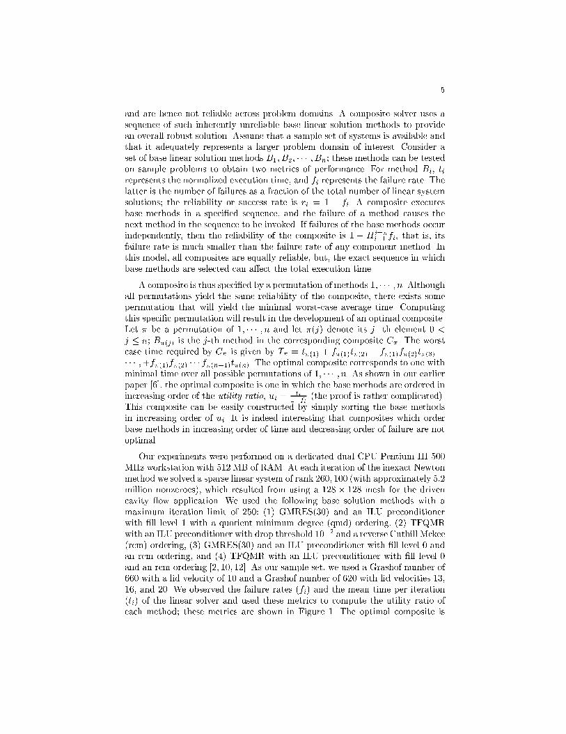
Our experiments were performed on a dedicated dual-CPU Pentium III 500MHz workstation with 512 MB of RAM. At each iteration of the inexact Newtonmethod we solved a sparse linear system of rank 260; 100 (with approximately 5:2million nonzeroes), which resulted from using a 128� 128 mesh for the drivencavity ow application. We used the following base solution methods with amaximum iteration limit of 250: (1) GMRES(30) and an ILU preconditionerwith �ll level 1 with a quotient minimum degree (qmd) ordering, (2) TFQMRwith an ILU preconditioner with drop threshold 10�2 and a reverse Cuthill Mckee(rcm) ordering, (3) GMRES(30) and an ILU preconditioner with �ll level 0 andan rcm ordering, and (4) TFQMR with an ILU preconditioner with �ll level 0and an rcm ordering [2, 10, 12]. As our sample set, we used a Grashof number of660 with a lid velocity of 10 and a Grashof number of 620 with lid velocities 13,16, and 20. We observed the failure rates (fi) and the mean time per iteration(ti) of the linear solver and used these metrics to compute the utility ratio ofeach method; these metrics are shown in Figure 1. The optimal composite is

6

denoted as CU and corresponds to base methods in the sequence: 2, 3, 1, 4. Wealso formed three other composites using arbitrarily selected sequences: C1: 3,1, 2, 4; C2: 4, 3, 2, 1; and C3: 2, 1, 3, 4.

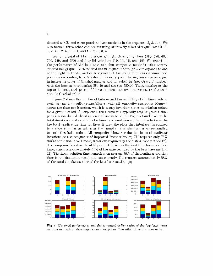
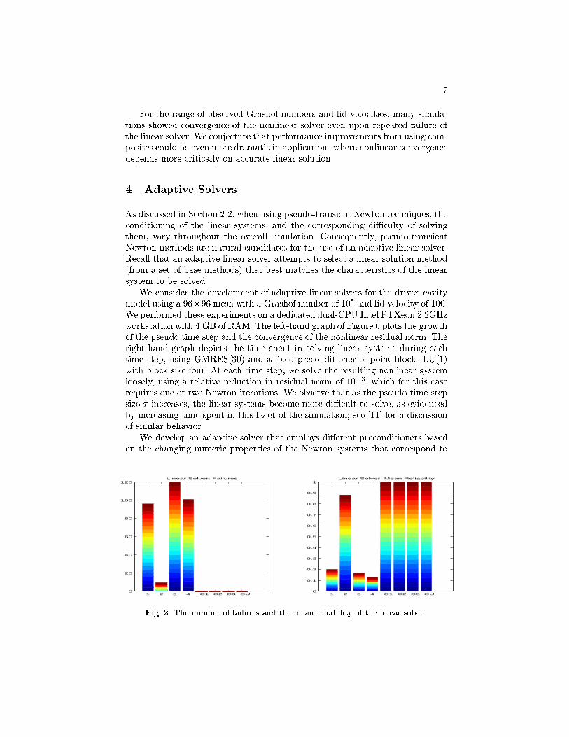
We ran a total of 24 simulations with six Grashof numbers (580, 620, 660,700, 740, and 780) and four lid velocities (10, 13, 16, and 20). We report onthe performance of the four base and four composite methods using severalstacked bar graphs. Each stacked bar in Figures 2 through 5 corresponds to oneof the eight methods, and each segment of the stack represents a simulationpoint corresponding to a Grashof:lid velocity pair; the segments are arrangedin increasing order of Grashof number and lid velocities (per Grashof number)with the bottom representing 580:10 and the top 780:20. Thus, starting at thetop or bottom, each patch of four contiguous segments represents results for aspeci�c Grashof value.

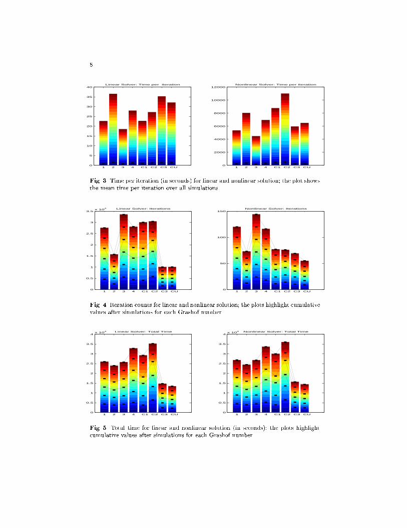
Figure 2 shows the number of failures and the reliability of the linear solver;each base methods su�ers some failures, while all composites are robust. Figure 3shows the time per iteration, which is nearly invariant across simulation pointsfor a given method. As expected, the composites typically require greater timeper iteration than the least expensive base method (3). Figures 4 and 5 show thetotal iteration counts and time for linear and nonlinear solution; the latter is thethe total application time. In these �gures, the plots that interlace the stackedbars show cumulative values at the completion of simulations correspondingto each Grashof number. All composites show a reduction in total nonlineariterations as a consequence of improved linear solution; CU requires only 75%(63%) of the nonlinear (linear) iterations required by the fastest base method (2).The composite based on the utility ratio, CU, incurs the least total linear solutiontime, which is approximately 56% of the time required by the best base method(2). The linear solution time comprises on average 96% of the nonlinear solutiontime (total simulation time) and consequently, CU requires approximately 58%of the total simulation time of the best base method (2).

1 2 3 40

5

10

15

20Number of Failures

1 2 3 40

1

2

3

4Reliability

1 2 3 40

1000

2000

3000

4000

5000

6000Iterations

1 2 3 40

1000

2000

3000

4000

5000

6000Total Time

1 2 3 40

1

2

3

4

5

6

7Time per iteration

1 2 3 40

5

10

15

20

25Utility Ratios

Fig. 1. Observed performance and the computed utility ratios of the four base linearsolution methods at the sample simulation points. Execution times are in seconds.

7

For the range of observed Grashof numbers and lid velocities, many simula-tions showed convergence of the nonlinear solver even upon repeated failure ofthe linear solver. We conjecture that performance improvements from using com-posites could be even more dramatic in applications where nonlinear convergencedepends more critically on accurate linear solution.

4 Adaptive Solvers

As discussed in Section 2.2, when using pseudo-transient Newton techniques, theconditioning of the linear systems, and the corresponding di�culty of solvingthem, vary throughout the overall simulation. Consequently, pseudo-transientNewton methods are natural candidates for the use of an adaptive linear solver.Recall that an adaptive linear solver attempts to select a linear solution method(from a set of base methods) that best matches the characteristics of the linearsystem to be solved.

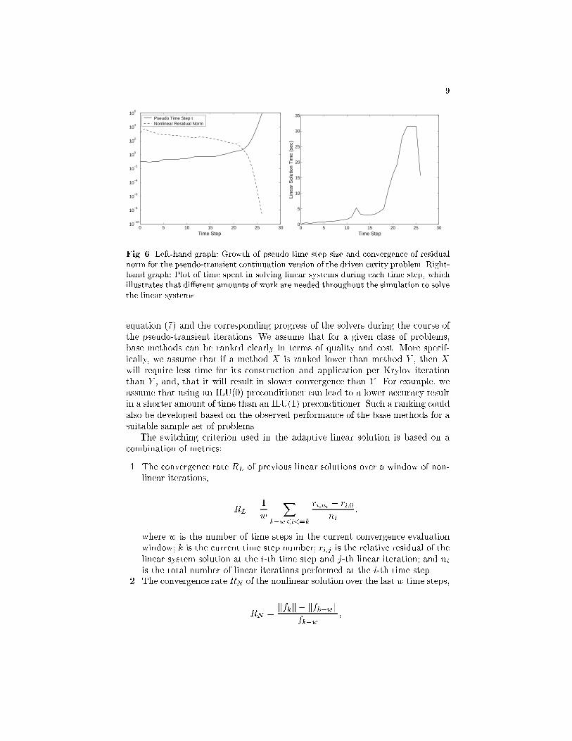
We consider the development of adaptive linear solvers for the driven cavitymodel using a 96�96 mesh with a Grashof number of 105 and lid velocity of 100.We performed these experiments on a dedicated dual-CPU Intel P4 Xeon 2.2GHzworkstation with 4 GB of RAM. The left-hand graph of Figure 6 plots the growthof the pseudo time step and the convergence of the nonlinear residual norm. Theright-hand graph depicts the time spent in solving linear systems during eachtime step, using GMRES(30) and a �xed preconditioner of point-block ILU(1)with block size four. At each time step, we solve the resulting nonlinear systemloosely, using a relative reduction in residual norm of 10�3, which for this caserequires one or two Newton iterations. We observe that as the pseudo time stepsize � increases, the linear systems become more di�cult to solve, as evidencedby increasing time spent in this facet of the simulation; see [11] for a discussionof similar behavior.

We develop an adaptive solver that employs di�erent preconditioners basedon the changing numeric properties of the Newton systems that correspond to

1 2 3 4 C1 C2 C3 CU0

20

40

60

80

100

120Linear Solver: Failures

1 2 3 4 C1 C2 C3 CU0

0.1

0.2

0.3

0.4

0.5

0.6

0.7

0.8

0.9

1Linear Solver: Mean Reliability

Fig. 2. The number of failures and the mean reliability of the linear solver.

8

1 2 3 4 C1 C2 C3 CU0

5

10

15

20

25

30

35

40Linear Solver: Time per iteration

1 2 3 4 C1 C2 C3 CU0

2000

4000

6000

8000

10000

12000Nonlinear Solver: Time per iteration

Fig. 3. Time per iteration (in seconds) for linear and nonlinear solution; the plot showsthe mean time per iteration over all simulations.

1 2 3 4 C1 C2 C3 CU0

0.5

1

1.5

2

2.5

3

3.5x 10

4 Linear Solver: Iterations

1 2 3 4 C1 C2 C3 CU0

50

100

150Nonlinear Solver: Iterations

Fig. 4. Iteration counts for linear and nonlinear solution; the plots highlight cumulativevalues after simulations for each Grashof number.

1 2 3 4 C1 C2 C3 CU0

0.5

1

1.5

2

2.5

3

3.5

4x 10

4 Linear Solver: Total Time

1 2 3 4 C1 C2 C3 CU0

0.5

1

1.5

2

2.5

3

3.5

4x 10

4 Nonlinear Solver: Total Time

Fig. 5. Total time for linear and nonlinear solution (in seconds); the plots highlightcumulative values after simulations for each Grashof number.

9

0 5 10 15 20 25 3010

−10

10−8

10−6

10−4

10−2

100

102

104

106

Time Step

Pseudo Time Step τNonlinear Residual Norm

0 5 10 15 20 25 300

5

10

15

20

25

30

35

Time Step

Line

ar S

olut

ion

Tim

e (s

ec)

Fig. 6. Left-hand graph: Growth of pseudo time step size and convergence of residualnorm for the pseudo-transient continuation version of the driven cavity problem. Right-hand graph: Plot of time spent in solving linear systems during each time step, whichillustrates that di�erent amounts of work are needed throughout the simulation to solvethe linear systems.

equation (7) and the corresponding progress of the solvers during the course ofthe pseudo-transient iterations. We assume that for a given class of problems,base methods can be ranked clearly in terms of quality and cost. More specif-ically, we assume that if a method X is ranked lower than method Y , then X

will require less time for its construction and application per Krylov iterationthan Y , and, that it will result in slower convergence than Y . For example, weassume that using an ILU(0) preconditioner can lead to a lower-accuracy resultin a shorter amount of time than an ILU(1) preconditioner. Such a ranking couldalso be developed based on the observed performance of the base methods for asuitable sample set of problems.

The switching criterion used in the adaptive linear solution is based on acombination of metrics:

1. The convergence rate RL of previous linear solutions over a window of non-linear iterations,

RL =1

w

X

k�w<i<=k

ri;ni� ri;0

ni;

where w is the number of time steps in the current convergence evaluationwindow; k is the current time step number; ri;j is the relative residual of thelinear system solution at the i-th time step and j-th linear iteration; and niis the total number of linear iterations performed at the i-th time step.

2. The convergence rate RN of the nonlinear solution over the last w time steps,

RN =kfkk � kfk�wk

kfk�wk;

10

0 5 10 15 20 25 3010

−10

10−8

10−6

10−4

10−2

100

102

104

Comparison of Base and Adaptive Linear Solvers

Time Step

Log(

10)

of N

onlin

ear

Res

idua

l Nor

m

Adaptive−ILU(k)ILU(0)ILU(1)ILU(2)ILU(3)

ILU(2)

ILU(0) ILU(3)

0 50 100 150 200 250 300 35010

−10

10−8

10−6

10−4

10−2

100

102

104

Comparison of Base and Adaptive Linear Solvers

CumulativeTime (sec)

Log(

10)

of N

onlin

ear

Res

idua

l Nor

m

Adaptive−ILU(k)ILU(0)ILU(1)ILU(2)ILU(3)

ILU(2)

ILU(0)

ILU(3)

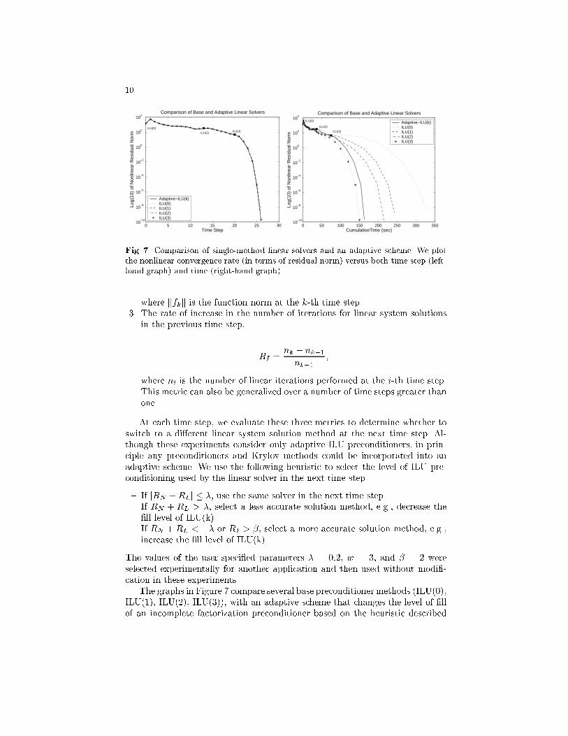
Fig. 7. Comparison of single-method linear solvers and an adaptive scheme. We plotthe nonlinear convergence rate (in terms of residual norm) versus both time step (left-hand graph) and time (right-hand graph).

where kfkk is the function norm at the k-th time step.3. The rate of increase in the number of iterations for linear system solutions

in the previous time step,

RI =nk � nk�1

nk�1;

where ni is the number of linear iterations performed at the i-th time step.This metric can also be generalized over a number of time steps greater thanone.

At each time step, we evaluate these three metrics to determine whether toswitch to a di�erent linear system solution method at the next time step. Al-though these experiments consider only adaptive ILU preconditioners, in prin-ciple any preconditioners and Krylov methods could be incorporated into anadaptive scheme. We use the following heuristic to select the level of ILU pre-conditioning used by the linear solver in the next time step.

{ If jRN +RLj � �, use the same solver in the next time step.{ If RN + RL > �, select a less accurate solution method, e.g., decrease the�ll level of ILU(k).

{ If RN + RL < �� or RI > �, select a more accurate solution method, e.g.,increase the �ll level of ILU(k).

The values of the user-speci�ed parameters � = 0:2, w = 3, and � = 2 wereselected experimentally for another application and then used without modi�-cation in these experiments.

The graphs in Figure 7 compare several base preconditioner methods (ILU(0),ILU(1), ILU(2), ILU(3)), with an adaptive scheme that changes the level of �llof an incomplete factorization preconditioner based on the heuristic described

11

above; all cases used GMRES(30). We plot convergence rate (in terms of residualnorm) versus both time step number (left-hand graph) and time (right-handgraph). The switching points for the adaptive scheme are marked on these graphsand indicate that the algorithm began using ILU(0), switched to ILU(2) at thethirteenth time step, and �nally switched to ILU(3) at the twentieth time step.We see that the overall time to solution for the adaptive solver is within 10% ofthe best base method, ILU(3), and the adaptive solver signi�cantly outperformsthe other base methods, being twice as fast as the slowest, ILU(0). Perhaps moreimportantly, the adaptive solver enables the simulation to begin with a methodthat is relatively fast yet not so robust, and then to switch automatically tomore powerful preconditioners when needed to maintain a balance in the linearand nonlinear convergence rates.

5 Conclusions and Future Work

Our preliminary results demonstrate the potential of multi-method compositeand adaptive linear solvers for improving the performance of PDE-based simula-tions. We continue to develop and evaluate multi-method solvers for large-scaleapplications from several problem-domains. Additionally, multi-method schemescan also be constructed for several other computational problems in large-scalesimulations, for example, discretization and Jacobian evaluation. We are alsoconsidering the e�ective instantiation of such schemes through advanced soft-ware frameworks that allow dynamic composition of software components [1,17].

Acknowledgments

We gratefully acknowledge Barry Smith, who enhanced PETSc functionalityto facilitate our work and participated in several discussions on the role anddevelopment of multi-method solvers.

References

1. R. Armstrong, D. Gannon, A. Geist, K. Keahey, S. Kohn, L. C. McInnes, S.Parker, and B. Smolinski, Toward a Common Component Architecture for High-Performance Scienti�c Computing, Proceedings of High Performance DistributedComputing (1999) pp. 115-124, (see www.cca-forum.org).

2. O. Axelsson, A survey of preconditioned iterative methods for linear systems ofequations, BIT, 25 (1987) pp. 166{187.

3. S. Balay, K. Buschelman, W. Gropp, D. Kaushik, M. Knepley, L.C. McInnes, B.Smith, and H. Zhang, PETSc users manual, Tech. Rep. ANL-95/11 - Revision2.1.3, Argonne National Laboratory, 2002 (see www.mcs.anl.gov/petsc).

4. S. Balay, W. Gropp, L.C. McInnes, and B. Smith, E�cient management of paral-lelism in object oriented numerical software libraries, In Modern Software Tools in

Scienti�c Computing (1997), E. Arge, A. M. Bruaset, and H. P. Langtangen, Eds.,Birkhauser Press, pp. 163{202.

12

5. R. Barrett, M. Berry, J. Dongarra, V. Eijkhout, and C. Romine, Algorithmic Bom-bardment for the Iterative Solution of Linear Systems: A PolyIterative Approach.Journal of Computational and applied Mathematics, 74, (1996) pp. 91-110.

6. S. Bhowmick, P. Raghavan, and K. Teranishi, A Combinatorial Scheme for De-veloping E�cient Composite Solvers, Lecture Notes in Computer Science, Eds. P.M. A. Sloot, C.J. K. Tan, J. J. Dongarra, A. G. Hoekstra, 2330, Springer Verlag,Computational Science- ICCS 2002, (2002) pp. 325-334.

7. S. Bhowmick, P. Raghavan , L. McInnes, and B. Norris, Faster PDE-based simula-tions using robust composite linear solvers. Argonne National Laboratory preprintANL/MCS-P993-0902, 2002. Also under review, Future Generation Computer Sys-tems,

8. R. Bramley, D. Gannon, T. Stuckey, J. Villacis, J. Balasubramanian, E. Akman,F. Berg, S. Diwan, and M. Govindaraju, The Linear System Analyzer, EnablingTechnologies for Computational Science, Kluwer, (2000).

9. T. S. Co�ey, C. T. Kelley, and D. E. Keyes, Pseudo-Transient Continuation andDi�erential-Algebraic Equations, submitted to the open literature, 2002.

10. I. S. Du�, A. M. Erisman, and J. K. Reid, Direct Methods for Sparse Matrices,Clarendon Press, Oxford, 1986.

11. A. Ern, V. Giovangigli, D. E. Keyes, and M. D. Smooke, Towards PolyalgorithmicLinear System Solvers For Nonlinear Elliptic Problems, SIAM J. Sci. Comput.,Vol. 15, No. 3, pp. 681-703.

12. R. Freund, G. H. Golub, and N. Nachtigal, Iterative Solution of Linear Systems,Acta Numerica, Cambridge University Press, (1992) pp. 57{100.

13. B. Fryxell, K. Olson, P. Ricker, F. Timmes, M. Zingale, D. Lamb, P. MacNeice,R. Rosner, J. Truran, and H. Tufo, FLASH: an Adaptive-Mesh HydrodynamicsCode for Modeling Astrophysical Thermonuclear Flashes, Astrophysical JournalSupplement, 131 (2000) pp. 273{334, (see www.asci.uchicago.edu).

14. C. T. Kelley and D. E. Keyes, Convergence analysis of pseudo-transient continua-tion. SIAM Journal on Numerical Analysis 1998; 35:508{523.

15. L. McInnes, B. Norris, S. Bhowmick, and P. Raghavan, Adaptive Sparse LinearSolvers for Implicit CFD Using Newton-Krylov Algorithms, To appear in the Pro-ceedings of the Second MIT Conference on Computational Fluid and Solid Me-chanics, Massachusetts Institute of Technology, Boston, USA, June 17-20, 2003.

16. J. Nocedal and S. J. Wright, Numerical Optimization, Springer-Verlag, New York,1999.

17. B. Norris, S. Balay, S. Benson, L. Freitag, P. Hovland, L. McInnes, and B. F. Smith,Parallel Components for PDEs and Optimization: Some Issues and Experiences,Parallel Computing, 28 (12) (2002), pp. 1811-1831.

18. X. Z. Tang, G. Y. Fu, S. C. Jardin, L. L. Lowe, W. Park, and H. R. Strauss, Resis-tive Magnetohydrodynamics Simulation of Fusion Plasmas, PPPL-3532, PrincetonPlasma Physics Laboratory, 2001.