The Role of Long-Term Contracting in Business Lending

The Role of Long-Term Contracting in Business

Lending*

Xiaoye (Phoebe) Tian†

April 21, 2021

Abstract

This paper studies inefficiencies arising from a lack of long-term contracting for small

business lending in less developed credit markets. Drawing a unique data from a Chinese

bank’s department that serves small and medium-sized firms, I find most firms repeatedly

take short-term loan contracts each year, and the main concern for the bank is default risk.

How, and to what degree can default risk be reduced by extending contracting horizon to

allow more flexible contractual arrangements? To analyze firm’s default incentives and de-

termination of contract terms, I develop a dynamic model where bank and firm repeatedly

interact through short-term lending contracts under uncertainty and learning. Learning

drives the dynamics of contract terms, which can explain observed features in the pane

data. Estimates of the structural model imply that over seventy percent of observed defaults

can be attributed to agency friction, i.e., willful borrower’s default. In my counterfactual

analysis, bank can design long-term contracts with state contingent terms. Optimal long-

term contracts improves efficiency through two channels: First, the intertemporal transfer

can alleviate agency frictions and reduce default incentives by front-loading prices. Sec-

ond, the intratemporal structure specifies price discount for firms with poor performance,

providing contingent insurance against risks from uncertainty. I find that long-term con-

tracting could reduce cumulative default rates by 17.15% and expand total outputs during

the sample period by 2.63%. The majority of the welfare improvement comes from the in-

tertemporal channel.

*I am indebted to Jean-François Houde and Ken Hendricks for their guidance and continuous support through-out the research process. I am also very grateful to Dean Corbae for his helpful comments and suggestions. Iwould also like to thank Lorenzo Magnolfi, Alan Sorensen, Ikuo Takei, Mark Rempel, Jason Choi, Anson Zhou,Andrey Zubanov, and participants at IO lunch workshop, IO seminar, IO-Finance Reading Group, and Finance-Macro-International Workshop at UW-Madison.

†Email: [email protected]. Department of Economics, University of Wisconsin-Madison.

1

1 Introduction

Small businesses play a central role in driving economic growth. The growth and development

of these firms, however, is sluggish in underdeveloped economies (Hsieh and Klenow, 2009,

2014). Since poor countries are also characterized by under-developed financial market, a vast

literature is devoted to the issue involving financial frictions and firm growth1. It is generally

recognized that financial restrictions can hinder firms’ ability to use inputs efficiently and affect

firm growth.2

Financial markets with relatively low levels of development often feature limited access to for-

mal financial services.3 One particular aspect largely overlooked by the literature is the lack of

long-term contracting in these markets.4 For example, while long-term financing agreements

like line of credits are common in US and other developed countries, they are rarely seen in

the lending market for small and medium-sized businesses in China.5 Short-term loans with

one year or less is the predominant type of loan product offered by commercial banks to small

businesses. As a result, small firms in China have to repeatedly negotiate short-term loans with

banks, which lead to excessive default risks and interest risks. The goal of this paper is to exam-

ine and quantify the benefits of long-term contracting on firm’s financing and development, in

the context of small and young firms in China.

Compared to short-term contracts which only specify lending terms for the current time pe-

riod, long-term contracts involve a predetermined schedule of future contract terms (which

can vary with time and borrower’s financial status). I focus on two benefits of such schedules

in long-term contracting. First, it alleviates the agency friction through its intertemporal struc-

ture. Business lending is characterized by the agency friction arising from borrower’s willful ex

post default, which poses a risk for the lender and distort the flow of capital. A long-term con-

tract can frontload prices and improve contract terms over time, thus lessening firm’s default

incentives and boosting access to credit. Second, a long-term contract accommodates rate re-

1See Buera et al. (2015) for an excellent review of the literature.2Cooley and Quadrini (2001), Huynh and Petrunia (2010), Buera et al. (2011), Arellano et al. (2012), Midrigan

and Xu (2014), among others.3For example, less access to savings accounts or bank loans, and lower levels of overall financial depth (King

and Levine, 1993).4The key difference between short-term contract and long-term contract is the presence of lender commit-

ments. In repeated short-term financing, the lender has the unilateral option of calling in the loan or raising inter-est rates at the beginning of each period. In long-term financing contracts, the bank commits to the preestablishedcontracts (Sharpe, 1991).

5There are many reasons behind the observed scarcity of long-term financing arrangement for small businesslending in China. One important reason is that traditional commercial banks, which are the major lenders inthis market, lack financial innovation. By contrast, newly emerging FinTech companies are starting to offer smallbusiness credit lines with longer contract maturity.

2

duction following realization of bad states, thus (at least partially) insure firms against negative

shocks.

This paper draws on a proprietary dataset from a Chinese bank, which keeps track of all loan

contracts with each of its small and medium-sized corporate customers. I can identify the be-

ginning of each firm’s lending relationship with the bank, and construct a complete panel of

loan contracts over a period of eight years. Several features of the data stand out. First, all con-

tracts are short-term, ranging from six month to one year (the majority is one-year). Second,

the ability of the bank to recover loans is a main concern, despite almost all loans are collater-

alized. This can be seen from the fact that 33.4% firms default during the sample period, and

that average coverage rate on defaulted loan is around half. Third, contract terms respond to

new information about firm performance: interest rates go up and loan size go down follow-

ing a poor performance. Furthermore, such responses become weakened over time, which is

consistent with Bayesian learning in an environment with incomplete information.

How much of the observed default is due to agency friction and how can it be reduced by longer

contracting horizon and more flexible contractual arrangements? To answer these questions,

I develop a dynamic structural model of firms (borrowers) and banks (lenders), in an environ-

ment featuring limited commitment and symmetric learning. In the model, firms are hetero-

geneous in their probability of getting negative productivity shocks, i.e., quality type. A firm’s

quality type is unknown to all banks and to the firm itself, but the distribution of quality type

conditional on observed firm characteristics is common knowledge. Banks compete at the be-

ginning of each period by offering single-period contracts, which consists of interest rates, loan

size, and collateral coverage. Firms make default decisions at the end of the period after pro-

ductivity and liquidity shock is realized. If default, the firm exits the market with a salvage value;

otherwise, it enters the next period with the updated belief based on this period’s productivity

performance.

The over-time variations in observed contract terms and firms’ performances, as well as their

comovements, are important in identifying the level of uncertainty and learning process, namely

type distribution and each type’s probability of negative shocks. The observed collateral cov-

erage, default rates and its comovements with shifts in funding costs, are critical in identify-

ing parameters related with the level of agency friction, namely transaction cost associated

with collateral, salvage value, and variance of liquidity shocks. A larger variance of liquidity

shock means higher liquidity risk that is innate to the business operation, which implies that

a larger fraction of observed defaults are due to intrinsic risks of the liquidity situation rather

than agency friction.

3

The model is estimated using generalized method of moments. Estimation results show several

important findings. First, while observed firm characteristics like industry account for most

dispersion in initial contract terms, conditional on firm observables, firms with low unobserved

type is five times as likely to perform poorly. Second, uncertainty about firm’s unobserved qual-

ity types lead to mispricing of default risks and misallocation of capital. Mispricing induces

three percent more defaults of high-type firms, and capital misallocation results in four percent

less capital taken by high-type firms. Learning over the seven-year period reduces mispricing

and misallocation by less than half. Third, collateral, as a tool to disincentivize default, is costly:

the transaction costs associated with collateral is around three percent of total collateral value.

Last but not least, I find that liquidity shock has a relatively large variance, although agency fric-

tion is still the more important source of inefficiency, accounting for more than seventy percent

of observed defaults. In absence of agency friction, total firm output would be fourteen percent

higher.

If counterfactually banks are able to make and commit to long-term contracts, how and to what

degree do firms benefit? Using estimates of the baseline model, I conduct a counterfactual exer-

cise where banks compete by offering long-term contingent contracts to firms. The long-term

contingent contract is essentially a schedule of contract terms as a function of future states,

where states encode information about the number of years into the contract, and firm’s perfor-

mances in each year of the contract. Such contract can be seen as an approximation of real-life

loan commitments. For example, in US, it is well expected that credit limit increases over the

time and good performances on a line of credit. And a large percentage of loans in US includes

performance-pricing provisions, which explicitly makes the interest as a function of the bor-

rowers financial condition (Asquith et al., 2005; Manso et al., 2010; Berg et al., 2016). Such state

contingent terms is the key component of long-term contracts in my counterfactual model.

I find that optimal long-term contracts improve efficiencies through two channels. First, the in-

tertemporal structure of the contract is such that lending terms become increasingly favorable

to firms over time, with declining prices and growing capital flow. Firms entering such con-

tracts are incentivized to stick to it and reap the benefits from good terms at the later periods.

Thus defaults incentives are reduced since default triggers a severance from the contract. Sec-

ond, under uncertainty about firm’s future profitability prospect, the long-term pricing scheme

specifies a price discount when firm’s financial situation deteriorates. This intratemporal struc-

ture serves like an insurance against adverse realizations, which not only enhances the overall

value of the contract to risk-averse firms, but also decrease default incentives of firms with poor

performance. In other words, it is a cross-subsidization from good-performing firms to others.

Ex ante, such cross-subsidization is favored by firms.

4

The two channels combined reduces cumulative default rates by 17.15%, increases firm size in

the last period by 1.23%, and expand total outputs during the seven-year period by 2.63%.6 It

recovers 31.46% of total welfare loss from agency friction and incomplete information. To fur-

ther see how the insurance channel contributes to the welfare improvement compared with the

intertemporal channel, I look at another counterfactual scenario where insurance is removed

from long-term contracts. I find that the reduction in defaults, increase in eventual firm size,

and expansion of total outputs are only slightly higher than the previous case, suggesting that

the intratemporal structure is less important than the intertemporal structure in term of curb-

ing default rates, promoting firm growth, and boosting overall firm outputs.

Related Literature This paper touches on three different fields, relating to the finance litera-

ture on optimal long-term financing contract, the IO literature on limited long-term commit-

ment, and the macroeconomic literature on the relationship between financial friction and firm

dynamics/growth. To my best knowledge this is the first study to look at the role of limited long-

term commitment in the dynamic financing contracts, and the consequences for firm growth.

In terms of methodology, my model is novel in that it examines corporate lending transactions

with rich specifications for firm heterogeneity, which makes it suitable for micro-level data.

There has been a long discussion in finance about the optimal long-term financing contracts

in which credit constraints emerge endogenously as a feature of the optimal contract design

(Gertler, 1992; Thomas and Worrall, 1994; Albuquerque and Hopenhayn, 2004; Quadrini, 2004;

Clementi and Hopenhayn, 2006; DeMarzo and Sannikov, 2006; DeMarzo and Fishman, 2007;

Biais et al., 2010; Boualam, 2018). In particular, Boualam (2018) apply model of optimal long-

term financing contracts to the US commercial loan market, where he argues long-term con-

tracts are available at a relatively low cost. My paper instead looks at countries where long-term

contracting is not easily accessible, and quantify the value of having long-term financing con-

tracts.

The discussion of limited long-term commitment in IO has been studied in the context of life or

health insurance (Cochrane, 1995; Hendel and Lizzeri, 2003; Atal, 2019). In Hendel and Lizzeri

(2003), the supply side (i.e., insurance companies) is able to commit but the consumers can-

not (i.e., they can switch), which leads to front-loading premiums in long-term contracts. This

paper finds that, when the supply side (i.e., banks) can commit, optimal long-term contracts

are also front-loaded. But the reason behind front-loading is completely different from Hendel

and Lizzeri (2003): Here front-loading is employed to alleviate agency friction arising from the

6Here I measure firm size by outputs, which is increasing in loan size. Cumulative default rates refers to thefraction of firms ever defaulted in the sample period.

5

borrower’s incentive to avoid repayment, while in Hendel and Lizzeri (2003) front-loading is a

result of a lack of consumer commitment. This paper thus complements the discussion of the

effect of a lack of long-term economic arrangements by examining a market characterized by

agency frictions.

This paper pertains to empirical studies of credit markets with agency frictions, such as Adams,

Einav, and Levin (2009), Einav et al. (2012), Crawford, Pavanini, and Schivardi (2018), Xin (2020).

In particular, Adams, Einav, and Levin (2009) and Crawford, Pavanini, and Schivardi (2018) in-

terpret a positive correlation of default and loan liability (conditional on observables) as moral

hazard in credit market. The agency friction in my paper fits into this (broad) definition of

moral hazard. It is akin to the type of “moral hazard” in Einav et al. (2012), i.e., willful default

after income/revenue is realized, as apposed to the kind of ex ante moral hazard in Xin (2020).

Compared to Einav et al. (2012) and Crawford et al. (2018), my model is different in that it is

in the setting of repeated lending transactions and estimated using a panel data on lending

transactions, while Einav et al. (2012) and Crawford et al. (2018) focus on one-time loan trans-

actions.7

This paper is also related to structural estimation of learning models (Ackerberg, 2003; Crawford

and Shum, 2005; Pastorino, 2019). Ackerberg (2003) and Crawford and Shum (2005) assume

the “signals” through which learning takes place is unobserved, while Pastorino (2019) treats

observed panel data on performance as a direct evidence of signals. My approach is similar to

Pastorino (2019) in that I also utilize observed measures of performance to pin down the belief

updating process. These papers are in the context of either single-agent dynamic problem or

dynamic problem with no agency frictions, I contribute to this slew of studies by estimating the

learning process in an environment with agency friction.

Finally, there is a vast literature on the relationship between financial frictions and entrepreneur-

ship (Cooley and Quadrini, 2001; Huynh and Petrunia, 2010; Buera et al., 2011; Arellano et al.,

2012; Midrigan and Xu, 2014; Buera et al., 2015), and this paper contributes by providing micro-

level evidence of how the friction in writing long-term contracts can affect the growth of small

firms through inefficient default choice and inefficient use of inputs.

The rest of the paper is organized as follows. Section 2 provides institutional backgrounds, and

describes key features and patterns in the data. Section 3 describes the model, Section 4 dis-

cuss identification concerns, specifies the empirical model, and estimates the model primitives.

7This is not saying that previous literature in this realm do not use dynamic models. Einav et al. (2012) and manypapers on residential mortgage loans analyze subsequent repayment behavior as dynamic programming problem.But the loan transaction between a lender and a borrower is one-time, which is where my paper differs.

6

Section 5 conducts the counterfactual analysis. Section 6 concludes.

2 Data and Institutional Background

2.1 China’s Banking Industry

The banking sector in China originated from a centralized system in 1949 when the People’s

Bank of China (PBC), as China’s central bank, governed both commercial bank businesses (e.g.,

deposits, lending, and foreign exchange) and central bank functions. Along with economic

opening policies being instituted by Deng Xiaoping in 1978, the banking system entered a pe-

riod of reform. In 1983, the PBC began to focus on national macroeconomic policy, monetary

stability, and economic development. At the same time, the big four commercial banks (i.e.,

the ICBC, ABC, BOC and, CCB) started to take over commercial bank businesses, and each was

specialized in a specific area. The Bank of Communications’ experience in reform and develop-

ment has paved the way for the development of shareholding commercial banks in China and

exemplified banking reforms in China (Gao et al., 2019a).

Between 1988 and 2005, twelve joint equity banks were established, mostly as SOEs or institu-

tions transformed from local financial companies. Although joint equity banks are also national

banks, unlike big five commercial banks, they usually focus on local business and operate on

a much smaller scale. By the end of the year 2013, as reported by China Banking Regulatory

Commission (CBRC)’s annual reports, the big five commercial banks dominate the market and

control for approximately 43.3% of the market share. On the other hand, joint equity banks

are much smaller and control for about 17.8% of the market share. The rest of the financial

institutions belong to the third tier such as municipal commercial banks.

2.2 Deregulation of Credit Controls and Interest Rates

The first step in deregulation of credit control is taken was 1998. Until then, the central bank

had controlled the lending of Chinese banks through binding credit quotas. This binding credit

plan system was formally abolished in 1998, replaced with an indicative non-binding credit

target. In other words, commercial banks in China are no longer required to provide loans

in compliance with state directives or policy targets. Instead, they are encouraged to allocate

funds “on the basis of proper credit assessments" and lend based on economic and commercial

considerations. This change in policy has been hailed by Chinese monetary authorities as an

7

important initial step in transforming the credit culture of Chinese banks (Xu et al., 2016).8

Lending rates in China have been substantially more liberalized than deposit rates through-

out the path of interest rate deregulation, starting with the interbank offered rate in the capital

market to be fully market-priced in 1996. From 1998 onward, the People’s Bank of China (PBC)

started to widen the floating band on banks’ interest rates. In 2004, the deposit rate floor and the

lending rate ceiling were eliminated for the major banks. The remaining lending rate floor was

gradually widened and eventually completely removed.9 In practice, the lending rate floor was

largely non-binding even before it was removed (Xu et al., 2016). Deposit ceiling was binding

(He and Wang, 2012), and it was not removed until October 23, 2015.

The day following October 23, 2015 marked the last change of benchmark lending rates until

this day. The benchmark lending rate refers to the official reference for lending rate published

by PBC. It served as a non-binding “guidance” on lending rates in the market, and had been

an active policy instruments. Prior to October 2015, changes in the benchmark lending rates

had been made by PBC10 at random dates, typically seven or eight times a year. After October

24, 2015, however, it seems that the benchmark lending rate has ceased to function as an ac-

tive policy instrument since no adjustment has been made so far; instead, the focus of PBC is

increasing on short-term money market rates, namely the 7-day interbank pledged repo rate

(DR007).11 This move is generally seen as part of interest rate liberalization that allowed PBC to

improve its policy framework (McMahon et al., 2018).

2.3 Data Description

This paper utilizes three sources of data from a Chinese bank: (1) loan contract and loan out-

come data, (2) (anonymized) corporate borrower data, and (3) internal rating data. The loan

contract data contains detailed information on loan contracts with corporate borrowers, in-

cluding a loan identifier, a firm identifier, date of origination, contract interest rates, loan size,

loan maturity, repayment frequency, types of collateral, value of each type of collateral, branch

8There are still signs of quantitative controls on bank credit, as the central bank employs an array of quantitativeinstruments aimed at controlling credit growth, such as yearly aggregate target levels for new loans and the use ofso-called window guidance which can be described as a form of moral persuasion aimed at controlling the sectoraldirection of lending (Okazaki, 2007).

9The lending rate floor was reduced to 0.9 times the benchmark official lending rate in October 2004, 0.8 timesthe benchmark lending rate in June 2012, 0.7 times in July 2012, followed by a complete removal in July 2013.

10These changes need to be approved by the State Council (China’s equivalent to a government cabinet) as well(McMahon et al., 2018).

11In the 2016, third-quarter Monetary Policy Executive Report, the PBC stated that “DR007 moves around theopen market operation 7-day reverse repo rate. The DR007 can better reflect the liquidity condition in the bankingsystem and has an active role to cultivate the market base rate”.

8

and sub-branch identifier. Loan outcome is an indicator of whether the loan is classified as a

nonperforming asset (NPA) as of June 2018. NPAs are listed on the balance sheet of the bank

after a prolonged period of non-payment and evidence of extremely low repayment probability.

They are typically viewed as loans that are in default.

The corporate borrower data used in this paper include the the borrowing firm’s industry code,

location (up to district level), size category, ownership type, date of incorporation, initial cap-

ital, and an initial assessment. The initial assessment is conducted by the bank when the firm

borrows for the first time. It is a categorical variable that summarizes all soft and hard informa-

tion that bank knows about the perceived quality of the firm at the beginning.

I also draw on data on bank’s internal ratings for loans. For each loan, banks in China are re-

quired to report a rating to CBRC on a monthly bases until the loan is off the bank’s balance

sheet. These ratings are assigned according to a five-category loan classification system, in

which there are five levels: 1 is the highest rating for the “normal” loans, 2 is for the “special

mentioned”, 3 is for the “substandard”, 4 is for the “doubtful” and 5 is for the “loss”. In this pa-

per, internal rating is defined as a dummy variable for whether the loan rating is normal or poor

(i.e., ratings from 2 to 5), as in Gao et al. (2019b). This method of classification is mainly based

on borrowers’ repayment ability, that is, their actual ability to repay principal and interests. As-

sessing this ability entails, for example, monitoring and analyzing the borrower’s changes in

revenue and profits, cash flow, financial position, management efficiency, etc. One bank can

request records of a borrowing firm’s past rating history from CBRC at low monetary costs. Al-

though banks report ratings every month until a loan is paid off, I can only observe one snap-

shot of the monthly ratings taken at the month of December in that corresponding year. I refer

to this as the internal rating on that loan.

The loan data is merged with firm data, which is then merged with the internal rating data with

loan identifier. The data includes the date of the first loan of each firm, thus enabling me to

identify the true beginning of the lending relationship. The end of my sample period is the end

of 2017.12

Sample Restriction For the purpose of this paper I restrict the sample to only small and medium-

sized young firms that first borrow from the bank only after the beginning of the sample period,

Jan 2, 2010. Specifically, the firm-level data has a categorical variable indicating firm size—

12I can observe data on contract terms up to the middle of 2018, but the outcomes on loans originated in 2018has not been recorded. So my final sample does not include those loans.

9

large, medium, small, which is defined according to a national criteria13. I define young firm

is firms whose age is less or equal to five at the first time of borrowing. In total, there are 6358

such firms in my sample.

Feature 1: Loan contract terms are negotiated annually. This is based on three observations

of the loan-level data. First, all of the loans are short-term loans: 80.63% of loan terms are one-

year, and the rest is between six-month to one-year. Second, on average 78.6% of firms borrow

only once in a given year, and among those who borrow more than once, the interest rates on

multiple loans originated in the same year are similar, in contrast with the relatively large year-

to-year variations on lending rates within a firm.14 Lastly, nearly all of the loans has one-time

repayment due at the end of the loan maturity.

Based on this feature, I aggregate the loan-level data to firm-year level. Specifically, for each

firm, I take the average interest rates and value of collateral, the sum of loan size, and the out-

come of the last loans within each year, and get a firm-level annual panel data on loans. In

total, there are 17518 observations on firm-year level. Summary Statistics of year one to seven

is shown in Table 14.

Feature 2: Repeated lending is common. To find out the longitudinal properties of the panel

data, I define the duration of the relationship as the difference between the last time it borrows

from the bank and the first time. Figure 2 shows the distribution of relationship duration. Three

quarters of firms borrow more than once, and the median duration is three years. For firms

who repay their last year’s loan, 70.09% of them come back and take a new loan. Firms who

default exit the sample.Among the firms who never default, 90.6% has been borrowing annually

without a gap, and 7.45% has had only one gap year in their borrowing history, with only 1.95%

firms have a two-year gap or longer.15

Feature 3: Default is a prominent source of risk despite common usage of collateral. There

are three types of collateral: securities, fixed-assets, and third-party guarantee, which are or-

dered in the perceived recoverability. In the sample, all of the loans are secured by at least

one type of collateral: 35.5% of loans only have third-party guarantee, 28.4% only pledge fixed-

assets, 23.97% pledge both fixed-assets and third-party guarantee, and the remaining 12% uses

13See the administrative rule at http://www.gov.cn/zwgk/2011-07/04/content_1898747.htm. This classi-fication rule defines the range of number of employees and annual revenues to qualify for a small-sized company,which varies by industry. For example, in the retail industry, a company with employment 5 to 20 and annualrevenue 10 to 50 million RMB (1.4 to 7.2 million USD) is classified as a small-sized company.

14On average the coefficient of variation of interest rates on multiple loans within the same year for the samefirm is 0.07.

15I cannot identify reasons of leaving for a firm who has not defaulted previously due to limitations of the data.

10

securities as collateral. In spite of ubiquitous collateral usage, the bank still faces significant

losses in the event of default. This is seen from the set of recovery rates on each type of col-

lateral, which is used by the bank to project risks. The recovery rate on third-party guarantee

is around 0.16, which can vary with the credibility of the guarantor. The recovery rate on fixed

assets is around half, varying with the specific type of assets. Securities has the highest recovery

rate due to its high liquidability, around eighty to ninety percent. I calculate the recoverable

value of collateral using the set of recovery rates provided by the bank and calculate the collat-

eral coverage ratio as the ratio between recoverable value of collateral and the loan amount. The

collateral coverage ratio is on average around 55%, which means that the bank’s expected loss

from default is around fifty cents per dollar of the loan. There is also considerable default risks:

around 33% of firms in my sample ends up with default over the period from 2010 to 2017.

Feature 4: For firms with good rating history, contract terms improve over the course of the

relationship. I define firms with good rating history as firms who do not have a single poor

rating in their entire rating history. In my sample, 76% of all firms have a good rating history.

Among those firms, I first regress contract terms (lending spread, loan size, collateral coverage)

on observed firm characteristics (industry code, location, size category, ownership type, date of

incorporation, initial capital, and an initial assessment), cohort fixed effects (i.e., fixed effects

of the first year of borrowing), monthly time fixed effects, and branch fixed effects, in order to

get the residuals.16 I then plot the residualized contract terms ( lending spread, loan size, collat-

eral coverage) over year in relationship, as shown in Figure 3. Overall, the residualized lending

spread and collateral coverage decreases with the year in relationship, while the residualized

loan size increases with the year in relationship. Alternatively, we can check the intertemporal

trend of contract terms within each firm. Utilizing the panel structure of the data, I run a re-

gression of contract terms (yi t = lending spread, loan size, collateral coverage) on the year in

relationship t controlling for firm fixed effects (αi ) and time fixed effects (ξt ):

yi t =β0 +β1t +αi +ξt +ei t (1)

Results are reported in the column (1) to (3) of Table 1 (where t stands for year in relationship).

On average, as relationship proceeds, lending spread drops by 2.83 bps per year, loan size in-

creases by 162,000 CNY (≈ 24 thousand dollars) per year, and collateral coverage ratio drops by

0.35 % per year. This suggest that contract terms in general become more favorable to firms

over the course of the relationship, in cases where the firm is never rated poorly.

16Lending spread is the difference between interest rates and deposit rate.

11

Table 1: Regression of Contract Terms on Past Performance and Year of Relationship

Firms w. good rating history Firms w. poor rating history

(1)LendingSpread

(2)LoanSize

(3)CollateralCoverage

(4)LendingSpread

(5)LoanSize

(6)CollateralCoverage

t -0.0282 0.162 -0.00350 -0.0120 0.0387 0.00836(-3.72) (8.81) (-1.99) (-1.53) (0.84) (1.07)

Poor Rati ng t−1 0.0399 -0.144 0.0162(3.15) (-2.38) (1.68)

t ×Poor Rati ng t−1 -0.00655 0.0267 -0.00797(-2.53) (2.51) (-2.17)

Observations 8328 8328 8328 2344 2344 2344

t statistics in parentheses. Other controls: firm fixed-effects, quarterly time fixed-effects.

Feature 5: A poor rating is associated with an adverse change in contract terms next period,

and such change attenuates over the course of the relationship. Let period t denote the year

in relationship. Suppose in period t a firm is rated poorly for the first time, then how will con-

tract terms respond in the next period? And how will such responses change with t? To see

this, I regress contract terms (yi t = lending spread, loan size, collateral coverage) on a dummy

variable indicating whether last period’s rating is poor (Poor Rati ng t−1), year in relationship t ,

and their interaction term t ×Poor Rati ng t−1, while controlling for firm fixed effects (αi ) and

time fixed effects (ξt ). The regression is run on firms who have at least one poor rating in their

history, and for each firm i , I keep observation t <= t∗i + 1 where t∗i is the first time firm i is

rated poorly.

yi t =β0 +β1t +β2Poor Rati ngi ,t−1 +β3t ×Poor Rati ngi ,t−1 +αi +ξt +ei t (2)

Results of the regressions are shown in column (4) to (6) of Table 1. For a firm who is rated poorly

in the first period, then on average its contract terms next period became tougher: lending

spread increases by around three bps, loan size go down by around one hundred and twenty

thousand CNY, collateral coverage ratio increases by around one percent. However, if a firm’s

first poor rating happens only in period t > 1, then the adverse changes on its contract terms

in the following period are not as large in magnitude as the previous case. In other words, new

information about the firm’s performance that arrives later in the relationship worsens contract

terms to a lesser degree.

In sum, Feature 1 suggests that observed loan contracts are short-term with annual negotia-

12

tions. Feature 2 suggests that there can be meaningful dynamics in the repeated lending con-

tracts. Feature 3 suggests that default risks are important considerations in this environment,

since default rates are relatively high and collateral is commonly used, which is typically seen as

an disincentive to defaults. Feature 4 and 5 together is consistent with a Bayesian learning pro-

cess, where poor ratings lead to more pessimistic beliefs about the firm’s profitability and higher

expected default risks, and it is reflected in tougher contract terms. A feature of Bayesian learn-

ing process is that new information happens later in the process updates beliefs less, which can

explain why contractual responses to poor ratings attenuate over time.

3 Model

Inspired by the patterns in the data, I develop a dynamic structural model of firms (borrowers)

and banks (lenders), in an environment featuring limited commitment and symmetric learning.

Limited commitment means the firm cannot pre-commit to repay; instead, it has the option

to choose to repay or default after observing revenue realizations. Symmetric learning means

banks and the firm are equally uninformed about the unobserved firm type, and they share

the same initial prior beliefs. In subsequent periods, they all update beliefs based on publicly

observed firm performances, so they share the same belief at any point in time.

The assumption about symmetric learning is admittedly a strong assumption, but perhaps

more justifiable in my case of young firms. These firms, or entrepreneurs, are just starting

out themselves, and do not necessarily accumulate too much private information to hide from

banks. On the other hand, banks have funded similar projects in the past and do not necessar-

ily know less about the future prospect than the firm. This assumption helps keep the model

tractable while allowing us to see how informational frictions arising from incomplete informa-

tion can affect the dynamics of contract terms as well as firm outcomes.

I solve for equilibrium short-term contracts, assuming banks do not have access to long-term

contracting because of high contractual costs. This assumption about the lack of long-term

contracting is based on the institutional settings in my observed market. Firms and banks do

not have formal binding long-term agreements that would commit the firm to future borrowing

or hold the bank accountable for its promises on future contract terms. They negotiate contract

terms on a yearly basis, and the observed contracts are mostly one-year term loans.

13

3.1 Model Setup

Time is discrete with infinite horizon. There are two types of infinitely lived agents: firms , and

banks. Agents share the same discount factor β ∈ (0,1).

Firms

Banks are risk neutral. Firms, or entrepreneurs, on the other hand, are risk averse. They operate

their firms in order to maximize their expected utility from consumption within each period,

where consumption is total output net any payment. Firms are assumed to be hand-to-mouth

without access to a storage technology, although this model can be easily generalized to allow

accumulation of capital.The flow utility u : R→ R satisfies standard regularity conditions: u′ >0, u′′ < 0, limx→0 u′(x) = ∞, and limx→∞ u′(x) = 0. Although many papers on dynamic debt

contracting assumes risk neutrality (with exceptions like Thomas and Worrall (1994), Boualam

(2018)), this paper adopts risk aversion to better represent young or distressed firms who lack

ability to diversify firm-specific risk.

Each firm has access to a production technology, but it is cashless initially and has to seek out

external financing in order to start production. When funded with capital k, a firm of quality

type θ ∈Θ and characteristics s ∈S can generate output

y = a f (k), a ∼G(·|θ, s)

where the function f is differentiable, strictly increasing and strictly concave, and satisfies

f ′(k) > 0, f ′′(k) < 0, f (0) = 0, limk→0 fk (k) = +∞, and limk→∞ fk (k) = 0.17 Productivity a of

a firm with type θ and characteristics s in each period t is a random draw from the probabil-

ity distribution G(·|θ, s), with the associated probability density function (or probability mass

function) denoted as g (·|θ, s).

Both quality type and firm characteristics s are related with the distribution of a firm’s produc-

tivity.18 Specifically, conditional on the same s, a higher value of θ means higher productivity in

the first-order stochastic dominance sense. Formally, if θ′ > θ, then G(a|θ′, s) ≥G(a|θ, s),∀a. In

other words, higher θ indicating higher quality.

17The production function abstracts from labor and can be viewed as a profit function that already accounts forthe optional choice of labor input and associated wages.

18In empirical specification, I let quality type θ and characteristics s play different roles in productivity distri-bution G . Conditional on the same θ, I assume s only moves the distribution G horizontally without changing itsshape.(Formally, that means for s′ 6= s, there exists a scalar b such that G(a;θ, s′) =G(a +b;θ, s′),∀a). On the otherhand, θ can change the shape of distribution G conditional on the same s. High θ means a more right-skeweddistribution G and thus higher expectation of productivity.

14

Firms have a choice of whether to repay the bank loan in each period. Following production,

an i.i.d utility shock ε associated with repaying the bank loan is realized. Realization of the

repayment shock ε is observed by the firm, based on which the repayment decision is made.

Repayment shocks ε are assumed to be independent of quality θ. The mean of ε is zero, and

the variance of ε is denoted σ. Repayment shocks ε can be interpreted, for example, as liquidity

shocks that makes loan repayment harder for the borrowing firm.

Note that this setup nests the standard optimal long-term debt contract model with endoge-

nous borrowing constraints (Albuquerque and Hopenhayn, 2004; Boualam, 2018) by setting σ

to zero. In this case there is no randomness in default behavior and it is possible to completely

prevent defaults by designing the contract subject to default-free constraint. In general, a pos-

itive σ introduces some randomness in firm’s default behavior, which allows positive default

rates in equilibrium.

Loan Supply and Information Structure

There are two banks in a competitive bank loan market.19 Each bank acts as an intermediary

channeling funds from depositors to firms at a funding cost c, and the funding cost is the same

for every bank. Abstraction from bank heterogeneity allows me to focus on how agency friction

and learning shapes the dynamics of contract terms. Funding cost c ∈ C follows a stochastic

process with transition probability Γc :C×C→ [0,1].

Information is symmetric among agents in this model. In the beginning, all agents, including

bank and the firm itself, do not know the firm’s quality type θ, but can observe firm character-

istics s. Their initial prior belief is given by the distribution of θ conditional on firm character-

istics s, i.e., agents have rational expectations. In subsequent periods, the realizations of firm’s

outputs, or productivity, are commonly observed, based on which they update their belief via

Bayes rule.

Formally, denote pt (θ) the belief that a given firm is of type θ at the beginning of period t (before

production takes place in this period). Suppose Λ(θ|s) is the true distribution of quality types

conditional on firm characteristics s. Then the initial prior p1 :Θ→ [0,1] is:

p1(θ) =Λ(θ|s).

Given period t belief pt , and this period’s productivity realization, at , we can find the updated

beliefs in t +1, pt+1 :Θ→ [0,1], by Bayes rule:

19We can think of the two banks as my bank (the bank in my data) and the competing bank.

15

pt+1(θ) = g (at |θ, s)pt (θ)∫θ′ g (at |θ′, s)pt (θ′)dθ′

(3)

This learning process where all agents share the same belief at any point in time is also known as

symmetric learning. Such deviation from the asymmetric information literature is partly driven

by my focus on young firms, where the entrepreneur does not have extensive experiences of

running this business and thus has fewer private information to hide from the bank. The bank,

as argued in (Manove et al., 2001), has funded many similar projects in the industry, and does

not necessarily have fewer knowledge about the prospect than the entrepreneur. Extensive

initial screening and close monitoring are also in place to garner comprehensive information

about her ability to produce profits in the process of running a firm.

Timing

Figure 1 describes the timeline of the model, which consists of two stages. Period 0 is the orig-

ination stage where banks compete by offering short-term contracts, and the firm chooses one

bank. The the firm-bank pair proceeds to the dynamic contracting stage (period t ≥ 1). In each

period, the order of events are as follows: First, capital is advanced and production takes place.

Then productivity is observed and used to update belief. Then repayment shock realize, after

which the firm makes repayment decision. The contract continues only when the firm repays;

otherwise the contract ends.

Lending Contracts

Contract offers are built from standard single-period lending contracts. A single-period lending

contract in period t consists of interest rate (plus one) rt ∈ R+, loan size kt ∈ R+, and collateral

coverage zt ∈ [0,1]. It stipulates the firm put up an asset worth zk as collateral when taking

out the loan. At the end of the period, either the firm repays r k to the bank, or, in the event of

default, the firm loses possession of this collateral to the bank.20

The use of collateral generally involves a variety of costs, which might include necessary legal

documentation, monitoring and/or insurance for the asset to maintain the collateral’s value at

the agreed level, as well as implicit costs for the borrower in being forced to relinquish discre-

20Here we think of collateral as coming from the firm’s illiquid assets, which is different from working capital. Ido not consider constraints on the total pledgeable assets that a firm might face, or how past bank loans might leadto accumulation of total pledgeable assets. These are interesting theory extensions, but extra data on firm’s assetsis needed to identify related parameters.

16

Period t

Banks offer single-period contracts

Firm chooses one bank

Capital isadvanced

Productivitya realizes

Firm drawsε shock

Nextperiod

Contract ends

Repay

Default

Figure 1: Timing

tionary use of the asset (Chan and Kanatas, 1985). Regardless of their origin, these costs can

be assumed to be a strictly increasing function of the value of the collateral. Without loss of

generality, I assume the costs is a fraction γ of the total value of collateral zk. Furthermore, I

assume the firms pay transaction cost.21 Note that transaction costs accrue when firms take out

the loan at the beginning of each period, regardless of whether they ended up defaulting or not.

What then happens to a defaulting firm depends on the larger economic institutional systems

in place, and here I summarize the various costs related with defaults in a reduced-form way

by assuming that a firm would lose a fraction 1−δ of firm value. Put it differently, a defaulted

firm has salvage value that equals δ times the future firm value if the firm has not defaulted. An

extreme case of δ= 1 is where default event does not make any dent on the a firm’s future value

and it can continue accessing the credit market seamlessly. And the case of δ= 0 is the opposite

situation where defaulting firms are excluded from credit market forever and completely cease

to produce.

In general an environment with higher δ gives the firms higher incentive to default since the

salvage value is higher. (Or equivalently, the costs of defaults are lower.) Thus, the parameter δ

determines the level of agency friction in place.22

21According to Chan and Kanatas (1985), in a competitive credit market with costly use of collateral, if lender andborrower can negotiate how to divide the transaction costs of collateral between them, the optimal solution is theborrower pays all transaction costs. Therefore I use this as an assumption to simplify the model.

22Parameterδ, γ, andσ can be different for firms with different characteristics s, as in the estimated specification.

17

3.2 Equilibrium Short-Term Contract

I consider an environment where long-term contracting is unaccessible. Alternatively, we can

think of this case as lacking long-term commitments, i.e., a firms can unilaterally leave the long-

term contract after period-t loan is resolved and borrow from the spot market instead,23 and a

bank might renege its previous promise on this period’s contract terms. In other words, banks

cannot make credible promises on future contract terms (i.e., promises on future terms cannot

be enforced in this institutional environment24), and firms cannot make credible promises on

future borrowing. They only choose contract terms for the current period.

An equilibrium short-term contract is a single-period contract that maximize the firm’s value

while subject to zero expected bank profits. This is a direct result from bank competition on

three dimensions: price (i.e., interest rates), loan size, and collateral coverage. To see this,

first consider the case where a contract brings positive expected profits to a bank (and to all

banks since banks are homogeneous). Another bank can undercut by lowering prices by a small

amount and win all the firms (which is the standard Bertrand competition logic), so it cannot

be the equilibrium contract. The contract cannot bring negative expected bank profit either, by

the bank rationality requirement. So the equilibrium contract must bring zero expected bank

profit. There can be many contracts that satisfy zero-profit constraint, and it turns out only the

one that maximize the firm value can be the equilibrium contract. If a bank offers a zero-profit

contract that does not bring the highest possible firm value, then another bank could optimize

the contract structure and achiever higher firm value while still earning infinitesimal positive

profit per contract, which attracts all firms. Thus, the equilibrium contract must bring the high-

est possible firm value while subject the zero expected bank profit.

Let W (pt ,ct ) and Π(pt ,ct ) denote the expected firm value and expected bank profits when the

belief of the firm’s unobserved type is pt and fund cost is ct in period t . To express bank profits

and firm value, we can first find the firm’s value of choosing to repay and default, as well as

the associated repayment probability (or, equivalently, the firm’s default probability) on a given

short-term contract (rt ,kt , zt ).

Given period t ’s realization of productivity at and repayment shock, εt , the value of choosing to

repay for a firm with characteristics s is

u(yt −γzt kt − rt kt

)−εt +βEt W (pt+1,ct+1)

23Walking away before resolving this period’s loan is just defaulting, which would lead to loss of collateral.24It is worth noting that the lack of enforcement is on future transactions, as well as default behaviors. But

conditional on default, the transfer of collateral can be enforced.

18

where Et W (pt+1,ct+1) is short for Ect+1

[W (pt+1,ct+1)|pt ,ct , at

]with next period’s belief pt+1

completely determined by pt and at through Equation (3). And γzt kt is the transaction cost

associated with collateral, which accrues to the firm at the beginning of this period.

If the firm chooses to default, it looses the value of collateral zt kt , so the firm’s value of choosing

to default is

u(yt − (1+γ)zt kt

)+βδEt W (pt+1,ct+1)

where δEt W (pt+1,ct+1) is the salvage value for a defaulted firm.

Thus, the probability that a firm repays the loan viewed at the beginning of period t can be

expressed as:

Φt (at ) ≡ Pr(εt ≤ u

(yt −γzt kz − rt kt

)−u(yt − (1+γ)zt kt

)+β(1−δ)Et W (pt+1,ct+1)∣∣∣at

)(4)

Note that the repayment probability is contingent on realized at , since default decision is made

after productivity realizations. Specifically it determines the next period’s belief pt+1.

Using this notation of repayment probability, we can express the bank’s expected profits at the

beginning of period t as:

Π(pt ,ct ) =−ct kt +Eat

[Φt (at )rt kt + (1−Φt (at )) zt kt

∣∣pt]

(5)

Finally, we can define the equilibrium firm value as W (·) that satisfies:

W (pt ,ct ) = maxr,k,z

Eat ,εt

[max

{u

(yt −γzt kt − rt kt

)−εt +βEt W (pt+1,ct+1),

u(yt − (1+γ)zt kt

)+βδEt W (pt+1,ct+1)}∣∣∣pt

](6)

s.t. 0 =Π(pt ,ct ) (7)

and the associated policy function r (pt ,ct ),k(pt ,ct ), z(pt ,ct ) constitutes the equilibrium con-

tract terms. Note that the expectation is over at and εt , both of which realize after the loan

origination. Productivity realization at determines next period’s belief pt+1. εt determines the

repayment/default choice (which are inside of the maximization operator).

19

4 Empirical Analysis

We now move to the empirical aspects of the model, stating with a more detailed discussion of

assumptions maintained in estimation, identification of the model, and the estimated specifi-

cation. Since I only observe firms borrowing from the sample bank, from now on, I denote by

t = 1 the first year that a firm borrows from the bank. Thus, t denotes the year of the firm-bank

lending relationship.

4.1 Preliminaries

I assume there are two quality types: High type (θH ) and Low type (θL).25 This means that the

belief can be summarized by only one scalar p, which is the perceived probability that a firm

is of, say, high type. It greatly simplifies the model while still maintain the essence of learning.

The true fraction of high type conditional on s is given by λs , which also constitutes the initial

prior belief for firms with characteristic s by assuming rational expectation.

The distribution of productivity conditional on s and θ is assumed to be a two-point distribu-

tion: a ∈ {as , as} with as strictly larger than as . Note that the support of a does not change with

the unobserved type θ. Otherwise, agents would immediately infer the firm’s type just after one

period. The event of realizing as given s is called a poor performance; and the event of realiz-

ing as given s is called a good performance. Firms’ performance outcomes are observed by the

econometrician.

Conditional on the same s, firms with different quality type θ have different probability of realiz-

ing as (and thus as). Specifically, the high type θH has a strictly lower probability of poor perfor-

mance (i.e., realizing as): g (as |θH , s) < g (as |θL , s).26(Or equivalently, g (as |θH , s) > g (as |θL , s).)

I allow firm characteristics s, which are known to banks and firms, to be unobserved by the

econometrician. It is, however, correlated with a set of firm-level variables X that is observed by

the econometrician. Specifically, I assume that firm characteristics falls into S discrete groups:

s = 1,2, ...,S (where S is known), and the distribution of s conditional on X is given by a known

function H(X ;η). So η is the set of parameters that determines the distribution of s.

In addition, the firm-level production function f (k) is assumed to be of Cob-Douglas form

f (k) = kα with decreasing returns to scale parameter α. And the period utility of entrepreneurs

is CRRA with coefficient of relative risk aversion ρ. I fix risk aversion parameter and discount

25The binary assumptions on unobserved types is also seen in Pastorino (2019), Xin (2020).26This is implied by the first-order stochastic dominance assumption (mentioned in the model section) in the

context of binary type and two-point distribution.

20

factor, so the remaining structural parameters in the econometric model includes:

1. the parameters of conditional distribution of θ types, {λs}Ss=1, and the parameters of the

marginal distribution of characteristic groups s: η;

2. the parameters of productivity distribution conditional on s groups and θ types,{as , as , g (as |θH , s), g (as |θL , s)

}Ss=1;

3. the parameters of variance of repayment shocks {σs}Ss=1, the parameter of the default costs

δ, and the parameter of transaction costs associated with collateral: γ;

4. the parameters of returns to scale α;

4.2 Identification

I start the discussion by considering how the structural parameters are identified conditional

on s. Then I discuss how the distribution of s is identified conditional on variables X that are

observed in data. Here I mostly provide heuristic identification arguments.

1. The observed response of contract terms to past performances helps determine how different

the high and low types are in terms of performances; or, more specifically, the ratio of g (a|θL) to

g (a|θH ).27 Consider an extreme case where high type will never realize a poor performance and

low type always realize poor performance (i.e., the ratio g (a|θL)/g (a|θH ) approaches ∞), then

types are completely learned after the first loan, which means that we would see contract terms

change from period one to two, but stay constant afterwards (conditional on funding costs).

As the other extreme case, the high type has almost the same probability of realizing a poor

performance as the low type (i.e., the ratio is near 1), then each observation of performance

does not update beliefs very much, and learning takes place slowly and over a long period of

time.28 This means that in the data, we would see contract terms’ responses to performances

have very slow rate of change over time.

The rate of change of contractual responses to performances is captured in the coefficient for

the interaction term, β3, of regression (2). Consider a group of firms who has at least on poor

27s is omitted here since we are conditional on the same s throughout this part. The ratio g (a|θL)/g (a|θH ) lies in(1,∞) by definition.

28This can be seen mathematically from the Bayesian rule:

pt = pt−1

pt−1 + (1−pt−1)g (a|θL)/g (a|θH )

When g (a|θL)/g (a|θH ) →∞, belief shrinks to 0 immediately; when g (a|θL)/g (a|θH ) → 1, belief hardly updates.

21

rating in their history, with some firms’ poor performance happens in the early years, and others

happened at the later periods of their relationships. If learning is fast, beliefs in later periods can

be hardly changed by any news, then this new performance information that arrived in the later

periods has way smaller effects on contract terms than if it arrived in the earlier periods, which

means the sign of β3 is opposite from β2 and the magnitude of β3 is large compared to that

of β2. On the contrary, when learning is slow, new information arrived in later periods can be

almost as important as in early periods, so we would expect β3 to be small in magnitude (but

still has the opposite sign than β2 as long as learning exits). From Table 1, we find that β3 does

have the opposite sign thanβ2 in all of the three regressions, suggesting that learning does seem

to take place. The magnitudes of β3 are relatively small compared to that of β2, indicating that

learning is still happening at the later half the relationship.

2. Once the ratio of g (a|θL) to g (a|θH ) is determined, the separate values of g (a|θH ) and

g (a|θL), as well as the parameter of θ-type distribution, λ, can then be identified from the first

two period’s performance data. Intuitively, this is because when there is only one type, the aver-

age firm performance in period-two should be similar to period-one, assuming sample attrition

for reasons other than defaults are exogenous. When the type distribution is, say, half high and

half low, since low types are more likely to perform poorly, and default probability conditional

on poor performance are higher, more low types drop out from the cohort than high types,

resulting in a positive selection. As a consequence, the second-period’s average firm perfor-

mance is better than the first-period, and the magnitude of improvement is informative of type

distribution. In addition, the levels of average firm performance helps pin down performance

distributions for each type.

We can also see this in a more formal way. Note that the mean of poor performance in period-

one is (conditional on s):

E [Poor Per fi 1] =λg (a|θH )+ (1−λ)g (a|θL) (8)

Suppose D1 is the fraction of defaulted firms at the end of the first period, which can be ob-

served from the data. Then the proportion of low types within these defaulted firms is given

by

η1 =(1−λ)g (a|θL)d 1

λg (a|θH )d 1 + (1−λ)g (a|θL)d 1

(9)

where d 1 is the probability of default conditional on poor performance (or low realization of

a) in the first period. Importantly, this probability is only determined by the belief held by the

22

firm after its first performance, not by the true type of the firm, since we assume the firm do

not observe its true type. In other words, if a high-type firm and low-type firm both realize a

poor performance in the first period, they will have the same belief when they make default

decision on the first loan, and thus they have the same default probability (conditional on s).

Thus the same period-one default probability conditional on poor performance appears on

both the numerator and denominator of Equation (9), so it can be canceled out, leaving η1 a

function of only g (a|θH ), g (a|θL),λ.

Given η1 and D1, we can find the proportion of low type at the beginning of period-two, 1−λ−D1η1, and the proportion of high typeλ+D1η1. So the mean of poor performance in period-two

is (conditional on s):

E [Poor Per fi 2] = (λ+D1η1)g (a|θH )+ (1−λ−D1η1)g (a|θL) (10)

Given data on firm performances, we can measure the right-hand side of Equation (8) and (10)

using data, and the left-hand side of the two equations can be re-written in terms of g (a|θL)/g (a|θH ),

g (a|θH ), and λ, in which only the later two objects are unknown. So they can be jointly deter-

mined by the two equations.

3. The parameter of default costs δ and the variance of repayment shock σ can be pinned down

by the levels of default rates and the response of default rates to funding costs. Intuitively, both

parameters can control the observed level of default rates, but σ also determines how “exoge-

nous” the default events are.

Consider an extreme case of σ close to infinity, then defaults becomes almost irrelevant with

the comparison of firms values associated with repayment and default, i.e., it is close to a ran-

dom event that happens exogenously to firms. On the other extreme, when σ is close to zero,

then default is almost deterministic, and it almost surely will not happen if the firm’s value of

repaying is strictly larger than the value of defaults. It follows that σ should determine how sen-

sitive defaults are with respect to exogenous variations in firm’s value of repay, say, variations in

funding costs which affect interest rates and repayment. Thus, co-movements of default rates

and funding costs can identifyσ. Onceσ is pinned down, the observed level of default rates can

then pin down the parameter of default cost δ since it controls the default incentive of firms.

4. The parameter of collateral costs can be identified by the observed usage of collateral after

pinning down δ and σ. The role of collateral in this model is to provide a disincentive for the

firm to default. Once the levels of default incentives are pinned down by δ and σ, the most

23

important factor affecting the usage of collateral is the associated transaction cost, which is

indicated by γ.

5. The returns to scale parameter α can be identified from the joint distribution of initial loan

size and funding costs. This is because conditional on initial beliefs (which is given by the true

distribution of types), higher α means higher sensitivity of loan size with respect to funding

costs.

6. The high and low realizations of productivity {a, a} can be identified from the joint distribu-

tion of loan sizes and performance history at the end of their relationships. Once we identified

the learning parameters, we can pin down the difference in beliefs for firms with different per-

formance histories at the end of the sample period, and how the difference in beliefs translates

into difference in loan sizes depend largely on the levels of productivity {a, a}, and returns to

scale parameter α. Once α is identified from the previous step, we can then identify {a, a}.

So far, the identification argument is conditional on firm’s characteristic group s. The (para-

metric) distribution of group s conditional on observed firm variables X can be pinned down

by the distribution of initial contract terms conditional on firms’ X , since initial contract terms

are completely determined by a firm’s s group. In other words, the pattern of how firms with

certain value of X tend to share similar initial contract terms helps identify the link between s

group and firm variables X , which is summarized in the set of parameter η.

4.3 Functional Forms

Repayment Shocks I assume the repayment shock εt has a normal distribution with mean

zero and variance σs .29

Firm Characteristics In estimation, I let the number of firm characteristic groups S = 3, which

means that a firm belongs to one of the three characteristic groups s = 1,2,3. I use ordered pro-

bit model to model the distribution of s conditional on X . Specifically, s = j ⇔ ηcj ≤ X ′η f + e ≤

ηcj+1, for j = 1,2,3. Here e is a standard normal random variable, η f is a set of linear coeffi-

cients associated with X , and {ηcj }4

j=1 is the set of cut points with ηc1 = −∞ and ηc

4 = +∞. In

other words, the distribution of characteristic groups conditional on X in given by P (s = j |X ) =Φ(ηc

j+1 −X ′η f )−Φ(ηcj −X ′η f ), whereΦ(·) is the standard normal distribution function.

To construct X , I consider the following six firm-level attributes: industry, firm size, region,

29The normal distribution assumption aids calculation of the term E [ε|r epay], which is a truncated mean. Sincethe expectation of truncated normal distribution has a simple analytical form, normal distribution is assumed forε.

24

registered capital, cohort, initial assessment. All variables except for the registered capital are

categorical, and registered capital is continuous. Thus I generate dummy variables for each

categorical variables, which add up to 20 dummy variables. In total, I have 20+1 variables for X .

Distribution of Productivity Conditional on Firm Type. Conditional on the same θ, firms

with different characteristics s have different supports of productivity distribution. I make two

simplifying assumptions with regard to how s affects the productivity distribution: First, firms

of the same quality type all share the same probability of success, regardless of their character-

istics s. In other words, g (as |θ, s) is the same across s, and thus I will drop s from the parenthesis

and denote it as g (as |θ). Second, I assume the difference between as and as does not vary with

s, and I define this difference as ∆a ≡ as − as . In other words, fixing θ, characteristics s only

horizontally shifts the distribution of productivity without changing its shape.

Measurement of Firm Performances The outcome of performances (whether good or poor)

drives the learning process. Formally, I define a variable Poor Per f to reflect this binary out-

come for a given firm i in a given period t : Poor Per fi t = 1{ai t = a}.

I use the internal ratings to measure firm performances. As mentioned in Section 2.3, banks

in China are required to compile monthly internal ratings on every loan that stands out on the

bank’s balance sheet. These dynamic internal ratings, by definition, directly reflect bank’s as-

sessments about the firm’s repayment ability. They are different from the actual loan outcomes:

banks often downgrade a firm’s internal rating before actual delinquency happens as a result of

close monitoring (Gao et al., 2019b).

Data used in this paper contains one snapshot of the monthly internal ratings on every loan.

Specifically, that snapshot is taken in December, which means that for loans that are due in,

say, next March, this rating is recorded three months ahead of the due date. I use observations

whose due date is at least three months ahead of December, in order to ensure that the internal

rating does not merely reflect the loan outcome; it contains valuable information that shapes

the bank’s belief about the firm’s quality. This way we have an internal rating on each firm i in

each period t . A questionable internal rating on a firm at period t is taken as an observation of

an Poor Per fi t = 1.

Lending Cost I use the benchmark one-year deposit rates as the empirical counterpart of c.

Using data on the deposit rates from 2009 to 2018, I discretize the data into four bins: 1.75%

,2.25%, 2.75%, 3.25%, and estimate the transition matrix, which is then transformed to the tran-

sition matrix for yearly frequency.

25

4.4 Estimation

The estimation is based on simulated method of moments. The set of parameters to be esti-

mated is listed in Table 2, which is collected in vector Ξ. Following Boualam (2018), discount

factor β is set to 0.9542, and the relative risk-aversion is set to 0.6.

Table 2: List of Parameters

Parameters to be Estimated Definition

{as}3s=1 High productivity realization for each characteristic group s

∆a Difference between high and low productivity realization

{λs}3s=1 Fraction of high type within each characteristic group s

η f ,ηc2,ηc

3 Coefficients and cut points in determining s

g (a|θh) Prob. of high type realize high productivity

g (a|θl ) Prob. of low type realize high productivity

{δs}3s=1 Default costs as a fraction of firm value for each s

{γs}3s=1 Transaction cost of collateral for firms in each s

{σ}3s=1 Variance of liquidity shock for firms in each s

α Returns to scale parameter

mc Bank’s marginal cost of lending (in addition to funding cost)

Given a vector of primitives Ξ, for each s ∈ {1,2,3}, I solve for the value function W s(p,c), asso-

ciated policy functions r s(p,c), k s(p,c), zs(p,c), as well as repayment probabilities conditional

on each performance outcomes.

Then for each firm i = 1 to N = 6358,

1. I draw its quality type θi , based on which I draw a panel of performance outcomes {per fi t }

for t = 1 to T = 7.

2. Based on the initial state of funding cost ci 1, I simulate a path of funding cost for T period

ahead: {ci t } for t = 1, ...,T .

3. I also draw the characteristic s that it belongs to based on its X . The s characteristics deter-

mines the initial prior belief pi 1, which, combined with the panel of performance outcomes,

completely determines the path of beliefs {pi t }.

4. Now we have funding costs and belief (pi t ,ci t ) for t = 1, ...,T , so we can apply policy func-

tions r s(p,c), k s(p,c), zs(p,c) to find the contract terms {ri t ,ki t , zi t } in each period.

26

5. The default probabilities can also be found using both (pt ,ct ) and the simulated firm perfor-

mance outcomes, based on which the default outcomes {di t } are drawn. Defaulted firms are

then removed from the simulated data following its default.

I estimate the primitive using method of moments estimator by minimizing the differences be-

tween model prediction and the data counterpart of the following moments conditional on

exogenous firm variables X : (1) contract terms and defaults oi t = {ri t ,ki t , zi t ,di t }; (2) firm

performance outcomes per fi t ; (3) covariance between firm performance and contract terms

and default per fi t × oi t ; (4) covariance between funding costs and contract terms and de-

fault ci ×oi t . Formally, let mi t (Ξ) = {oi t , per fi t , per fi t ×oi t ,ci ×oi t

}, and its data counterpart

m = {oi t , ˆper f i t , ˆper f i t × oi t , ci t × oi t

}, then the moment restrictions used in the estimation

are (detailed lists are in Table 15):

g t (Ξ) = E{i } [mi t (Ξ)−mi t |Xi ] ,∀t = 1, ...,T (11)

I implement two-step generalized method of moments where I estimate the model using iden-

tity weighting matrix and obtain an estimator Ξ1. Using the estimator, I obtain the optimal

weighting matrix, Γ, and solve for Ξ by

Ξ= argminΞ

g (Ξ)Γg (Ξ)

where g (Ξ) = {g t (Ξ)}Tt=1. In total, I have 21 covariate vectors and 21× (28+7+28+28) = 1911

moment restrictions to estimate 35 parameters.

5 Estimation Results

In this section, I first discuss my parameter estimates. I then provide several pieces of evidence

to evaluate the model fit. I report the parameter estimates in Table 3. Panel A of Table 3 shows

estimates for parameters that vary across characteristic group s, which includes the high real-

ization of productivity as , the fraction of firm value that can be salvaged after a firm defaults,

δs , the fraction of high type firms conditional on s, λs , and the variance of liquidity shock σs . It

implies that there is considerable firm heterogeneity. The relatively large range in as translate

into large range in initial loan sizes: ranging from 2.43 to 8.93 (in millions RMB). The equilib-

rium default probabilities also have a wide range (1.3% to 12.03%), largely due to the relatively

large variations in δs and σs across s.

Panel B of Table 3 shows estimates for parameters that do not vary across characteristic group

27

Table 3: Parameter Estimates

Panel A: Parameters varying across characteristics s

as δs λs σs

s = 1 2.679 0.920 0.399 3.055s = 2 3.261 0.937 0.486 4.062s = 3 4.187 0.945 0.471 2.210

Panel B: Parameters that do not vary with s

∆a g (θh) g (θl ) α γ mc

0.702 0.974 0.867 0.607 0.032 0.015

s, which includes the difference between high and low realizations of productivity δa, the high-

quality-type’s probability of realizing high productivity, g (θh), and the low-type’s probability of

realizing high productivity, g (θl ), the return-to-scale parameter, α, the transaction cost asso-

ciated with collateral, γ, and the constant marginal cost of lending mc. Reading from g (θh)

and g (θl ), the high-type has a 2.6% change of poor performance, while it is 13.3% for the low-

type. The transaction cot associated with collateral is around 3% of the collateral value, which

is close to what credit guarantee companies charge on an annual basis.30 The marginal cost of

lending is estimated to be 1.5%, which is lower than the estimated “profit rate” 2.2% in Porter

et al. (2009) since Porter et al. (2009) does not take into account expected default costs.

5.1 Model Fit

The model predicts five observed variables (interest rates, loan sizes, collateral requirement,

firm performances, and default) over a period of seven years. I first check how do these variables

track the ones observed in the data over the seven years across all firms, and then break down

by different firm characteristics. The results are shown in Table.

Another important aspect of the model of the co-movement of firm performance and contract

terms. Specifically, how contract terms respond to new information of firms performance, and

how these responses change over time, speak directly to the speed of learning process. To sum-

marize this information succinctly, I use firm fixed effect model to regress contract terms on

years of relationship t , indicator of poor performance in the previous period, Poor Rati ng t−1,

and the interaction term t ×Poor Rati ng t−1, as in Equation (2). I conduct this regression for

firms who never had a single poor performance in their history (in which case the variable

30See Li and Lin (2017) for details on credit guarantee companies in China.

28

Table 4: Model Fit: Contract Terms, Performance, and Loan Outcomes

tr k z Performance Default

Data Model Data Model Data Model Data Model Data Model

1 7.043 7.236 4.482 4.822 0.573 0.556 0.081 0.085 0.040 0.0562 7.051 6.986 5.009 4.902 0.573 0.554 0.085 0.088 0.066 0.0603 6.826 6.728 5.371 4.991 0.570 0.551 0.084 0.089 0.081 0.0634 6.577 6.511 5.839 5.085 0.568 0.548 0.082 0.082 0.051 0.0515 6.420 6.366 6.485 5.165 0.565 0.546 0.089 0.085 0.079 0.0476 6.165 6.246 7.120 5.237 0.560 0.544 0.083 0.087 0.050 0.0517 6.004 6.136 7.572 5.314 0.535 0.542 0.089 0.087 0.080 0.049

Average 6.863 6.643 5.195 5.055 0.567 0.553 0.085 0.086 0.058 0.054

Table 5: Regressions of Contract Terms on Past Performance: Using Simulated Data

Firms w. good rating history Firms w. poor rating history

(1)LendingSpread

(2)LoanSize

(3)CollateralCoverage

(4)LendingSpread

(5)LoanSize

(6)CollateralCoverage

t -0.00531 0.0119 -0.000192 -0.00508 0.0126 -0.000201(-64.31) (64.30) (-114.01) (-20.10) (29.28) (-19.46)

Poor Rati ng t−1 0.0677 -0.120 0.00198(27.92) (-28.94) (20.01)

t ×Poor Rati ng t−1 -0.000220 -0.00621 0.000156(-0.45) (-7.42) (7.77)

Observations 18195 18195 18195 7613 7613 7613

t statistics in parentheses. Other controls: firm fixed-effects, funding costs fixed-effects.

Poor Per ft−1 and its interaction term with t will be omitted, and we will only compare the rate

of change of contract terms over time), and for firms who have at least one poor performance in

their history (again for these firms I keep observation t <= t∗i +1 where t∗i is the first time firm

i is rated poorly). Results are shown in Table 5.

The signs of coefficients in the regression using the simulated data are in line with empirical

results in Table 1, where we see a decline of lending spreads and collateral coverage, as well as

a gradual growth of loan size over the course of relationship for the firms who has never had a

poor rating (which are overwhelmingly high type). As for firms who performed poorly in period

t , the interest rate and collateral coverage next period is likely to go up, and loan size is likely to

go down in the next period.

29

5.2 Inefficiencies from Agency Friction and Incomplete Information

In the estimated model, there are two sources of inefficiency: incomplete information and

agency friction (or limited commitment). Incomplete information (or uncertainty) refers to the

fact that banks and the firm do not know the true θ type of the firm, which leads to a mismatch

of contract terms and firms: firms are assigned contract terms that are not optimal for their

true types. Although learning could reduce uncertainty and alleviate the implications from in-

complete information in subsequent period, the reduction might not be complete. To see the

inefficiencies cause by incomplete information, I consider the counterfactual case with full in-

formation, where firm types are fully known to both the bank and the firm from the beginning.

In this case, the firm’s value function is type-specific, and dynamics in contract terms are not

driven by learning.

Agency friction comes from the fact that firms cannot commit to repay; instead, firms have a

choice of whether to repay or default based on realized revenue and liquidity shocks. This can

also be viewed as a form of ex post moral hazard (Xin, 2020). To see how contract terms and de-

fault rates are different if there was no agency friction, I consider the planner’s problem, where

the repayment behavior can be enforced by the contract. This means that, in the planer’s con-

tracting problem, choice variables not only include (r,k, z), but also repayment policy (repay

or default). For example, in the case with full information and no agency friction, the contract

would be given be solution to the following problem of maximizing the joint value between firm

and bank subject the the bank earning zero profit:

Vθ = maxr,k,z

E max{

u(y −γzk − r k

)+ r k +βVθ︸ ︷︷ ︸vrepay

−ε,u(y − (1+γ)zk

)+ zk +βδVθ︸ ︷︷ ︸vdefault

}− ck

s.t. 0 =−ck + r k −D(r − z)k

where default probability D ≡ 1−Φ(

vrepay−vdefault

σ

).

I calculate the (counterfactual) short-term contracts in four scenarios: (1) no agency friction

and full information; (2) no agency friction and incomplete information; (3) with agency fric-

tion and full information; (4) with agency friction and incomplete information (the estimated

baseline model). For each firm, I find the associated cumulative default probability over the

seven-year period, total amount of capital and output taken over the seven-year period, the

firm size measured by output in the last period, and the initial firm value in the four equilib-

rium. Summary of these statistics by firm quality type is show in Table 6.

Comparing column (3) with column (4), we can see that incomplete information leads to misal-

30

Table 6: Comparisons Across Baseline Model, Models with One or Neither Source of Inefficiency

ScenarioBenchmarks Baseline

(1) (2) (3) (4)No AF No AF AF AF

Full Info. Inc. Info. Full Info. Inc. Info.

High-Type Firms

Cumulative Default Prob. .0877069 .0968651 .3237055 .3325114Total Capital 37.72948 36.20978 32.05138 30.71789Total Output 65.62923 63.9358 56.94183 55.4055Final Size 5.571345 5.380186 5.261407 5.071709Firm Value 88.68119 87.42284 87.55135 86.39585

Low-Type Firms

Cumulative Default Prob. .0934925 .0863882 .316283 .3117363Total Capital 33.13112 34.22402 28.31473 29.27848Total Output 58.12727 59.32193 50.78448 51.87864Final Size 4.898396 5.039846 4.612279 4.751198Firm Value 84.28747 85.30146 83.33981 84.25609

All Firms

Cumulative Default Prob. .0909091 .0910664 .3195974 .3210129Total Capital 35.1844 35.11071 29.98323 29.92121Total Output 61.47708 61.38213 53.53389 53.45347Final Size 5.198884 5.191816 4.90213 4.894314Firm Value 86.24937 86.24871 85.22037 85.21154

31

location of capital: high-types in baseline case are assigned lower capital than the full informa-

tion case as in column (3), whereas low types in baseline case are assigned higher capital than

the full information case. This mismatch of capital and firm productivity leads to lower over-

all outputs. In addition, there is an issue of mispricing due to incomplete information, where

high-types in baseline case are charged with higher interest rates than the full information case,

and low-types are charged with lower interest rates than the full information case. Such mis-

pricing of default risks and misallocation of capital leads to negative impacts on outcomes of

high-type firms, as shown in Figure 4. Learning, however, can reduced the negative impacts

over the course of the relationship to some degree. But at the end of the period, we still see

around half mispricing and misallocation compared to the initial period, as shown in Figure 5

and Figure 6.31

Comparing column (2) with column (4), we can see that in the benchmark scenario with no

agency friction (i.e., in the planner’s problem), default would be extremely rare, and capital flow

would be significantly enhanced. Specifically, the number of defaulted firms would be 71.63%

fewer than the baseline case, and total output would be 14.83% higher. In other words, the bor-

rowing constrains in the baseline case is largely due to agency friction. In total, agency friction

accounts for the vast majority of total welfare loss from both agency friction and incomplete

information.

6 Long-Term Financing Contracts

In this section, I consider the counterfactual scenario where long-term contracting is available,

and banks compete by offer long-term contracts. I start from a model with two-period con-

tingent contracts to show features of the optimal long-term contracts and explain my solution

method. Then I describe the multi-period contingent contracts and the results from my coun-

terfactual simulation exercises, like how firm outcomes are different under long-term contracts

compared to the short-term contracts.

6.1 Two-Period Contingent Contracts

To better illustrate the how long-term contracts work, I begin with the simplest case of long-

term contingent contract — two-period contract. Suppose banks offer two-period contingent

31Here I measure mispricing by (r C Ii /ri − 1)× 100% where r C I is interest rate in the counterfactual scenario of

complete information andr is interest rate in the baseline model. I measure misallocation of capital by (kC Ii /ki −

1)×100%, where kC I is loan size in the counterfactual scenario of complete information, and k is loan size in thebaseline model. Mispricing in the initial period is ≈ 1.7%, and misallocation of capital in the beginning is ≈ 4.8%.

32

contracts to new firms at the beginning of period one, and such contracts stipulate lending

terms in the first period, as well as the state-contingent lending terms of the second period. Af-

ter the two-period contract ends, a firm enters the infinite-horizon short-term lending market,

where competition takes place as described in the previous section. In other words, the thought

experiment I engage here is about providing long-term contracts at the beginning of a firm’s life,

and see how it affects the firm outcomes compared to the baseline model where firms are born

into a short-term lending market.

In this model, the banks compete at the beginning of period one by offering a two-period con-

tingent contract. Let lt denote the lending terms in period t , i.e., lt = (rt ,kt , zt ). Then the two-

period contract can be written as{l1, l2(p2,c2)

}where the second-period terms l2 is a function

of state variable (p2,c2).

I consider two-period contracts that are are binding conditional on repayment, meaning that

as long as the first-period loan is repaid by the borrower, then second-period borrowing activity

must take place according to the lending terms pre-determined in the contract. Specifically,

it implies that the lender cannot renege on the second-period terms and the borrower cannot

switch, if the first-period loan is repaid. If the borrower defaults on the first-period loan, then

the contractual relationship breaks and the firm receives scrap value that equals to a fraction δ

of its equilibrium firm value in the short-term lending market.

By the same logic as before, Bertrand equilibrium in this model results in maximization of firm’s

value subject to the zero profit condition. However, zero profit condition in this case means that

a bank expects the overall profit over the course of the long-term contract is zero, as apposed to

zero profit expected within each period. In other words, it is possible that the first-period ex-

pected profits are positive (negative), and the ex-ante second-period profits are negative (posi-

tive). This is because the binding long-term contract implies that there is no competition from

outside banks at the beginning of the second period, thus the second-period expected profit in

each possible state is no longer constrained to zero.

To succinctly state the problem solving for the equilibrium long-term contract, I first define a

few objects. Let U (lt ; at ) and U F (lt ; at ) denote the firm’s flow utility in period t for repayment

and default, respectively. They are functions of this period’s lending terms lt as well as the

realization of productivity at which determines the level of outputs.

U (lt ; at ) = u(yt (at )−γzt kt − rt kt

)U F (lt ; at ) = u

(yt (at )− (1+γ)zt kt

)

33

Using U (lt ; at ) and U F (lt ; at ), we can express the firm’s utility at the beginning of t = 2 as a

function of the second-period lending terms l2 and state variables p2, c2:

w2(l2, p2,c2) = Ea2,ε2

[max

{U (l2; a2)−ε2 +βE

[W (p3,c3)|a2

],

U F (l2; a2)+βδE[W (p3,c3)|a2

]}∣∣∣p2,c2

](12)

where W (·, ·) is firm’s value function in the short-term lending equilibrium. Here we maintain

the same assumption as the baseline model with regards to defaults: defaulting firms receive

scrap value that equals to a fraction δ of the firm value W .

It follows that default probability in the second period conditional on realization of a2 can be

written as

Φ2(l2, p2,c2; a2) = Pr(ε2 ≤U (l2, a2)−U F (l2, a2)+β (1−δ)E

[W (p3,c3)|a2, p2,c2

])(13)

Using the default probability function, we can find the expected bank profit for the second-

period:

π2(l2, p2,c2) =−(c2 − z2)k2 +Ea2

[Φ2(l2, a2, p2,c2) (r2 − z2)k2

∣∣p2]

(14)

At the beginning of the first period, for any given lending policy in period 1 and period 2, (l1, l2),

we can express firm’s expected utility as a function of l1, l2 as well as state variables (p1,c1):

w1(l1, l2, p1,c1

)= Ea1,ε1

[max

{U (l1; a1)−ε1 +βE

[w2

(l2, p2,c2

) |a1]

,

U F (l1; a1)+βδE[W (p2,c2)|a1

]}∣∣∣p1,c1

](15)

The difference in future values for the choice of repayment and default comes from the assump-

tion that defaults break the long-term contract and leave firm with a scrap value that equals to a

fraction δ of the firm value W . This leads to the following expression for the default probability

in the first period conditional on a1:

Φ1(l1, l2, p1,c1; a1) ≡ Pr(ε1 ≤U (l1, a1)−U F (l1, a1)+βE

[w2

(l2, p2,c2

)−δW (p2,c2)|a1, p1,c1])(16)

34

Thus the bank’s expected profit over the two periods is

π1(l1, l2, p1,c1) =−(c1 − z1)k1 +Ea1

[Φ1(l1, l2, p1,c1; a1) (r1 − z1)k1 +βE

[π2(l2, p2,c2)|a1

]∣∣p1,c1]

(17)

6.1.1 Original Problem

The original problem that a bank solves to obtain lending terms of the two-period contract in

the equilibrium is the following:

maxl1,l2(p2,c2)

w1(l1, l2(p2,c2), p1,c1

)s.t. 0 =π1

(l1, l2(p2,c2), p1,c1

)(18)

In other words, the bank chooses lending terms of the first period, l1, as well as second-period

terms contingent on state (p2,c2), that maximizes firm’s utility subject to zero expected profits

over the course of the two periods.

In the case where productivity at has a two-point distribution, then conditional on p1, next

period’s belief p2 has two possible values, p2(p1|a1 = a

), and p2

(p1|a1 = a

). Continuing the as-

sumption that ct takes four values, then there are 2×4 = 8 states for the second period. Since

lending terms l include three variables, r,k, z, in total there will be 3+8×3 = 27 choice variables

in this problem. And if we later extend the two-period contracts to multiple periods, the num-

ber of choice variables will explode. Thus, in this paper I consider an alternative approach to

solve for equilibrium long-term contracts.

6.1.2 Transformed Problem

Inspired by Albuquerque and Hopenhayn (2004), I transform the problem into one where the

lender chooses a summary statistics for future contract instead of fully spelling out each lending

term. This also helps forming a recursive representation of the original problem (18).

Note that given each state in period two, (p2,c2), for a certain level of expected bank profits π,

there is a unique solution to the constrained maximization problem of firm value subject to the

bank’s expected profit equal to π, and the maximum firm value is defined as W2(π, p2,c2):

W2(π, p2,c2) ≡ maxl2

w2(l2, p2,c2) s.t. π=π2(l2, p2,c2) (19)

35

Using π as an “index” for second-period contract contract contingent on the state (p,c), I re-

write the period-one objects (15)-(17) using π instead of l2: (I suppressed the parenthesis of π

in (15’) and (16’))

w1(l1, π, p1,c1) = E[

max{U (l1; a1)−ε1 +βE

[W2

(π(p2), p2,c2

) |a1]

,

U F (l1; a1)+βδE[W (p2,c2)|a1

]}∣∣∣p1,c1

](15’)

Φ1(l1, π, p1,c1; a1

)= Pr(ε1 ≤U (l1, a1)−U F (l1, a1)+βE

[W2

(π, p2,c2

)−δW (p2,c2)|a1, p1,c1])

(16’)

π1(l1, π, p1,c1) =−(c1 − z1)k1 +Ea1

[Φ1

(l1, π, p1,c1; a1

)(r1 − z1)k1 +βE

[π(p2,c2)|a1

]∣∣p1,c1](17’)

Thus, at the beginning of period one when banks make contract, instead of choosing three

lending terms for each state of period two, they choose an index π for each state of period two:

maxl1,π(p2,c2)

w1(l1, π(p2,c2), p1,c1

)s.t. 0 =π1

(l1, π(p2,c2), p1,c1

)(20)

The optimal choice of π corresponds to a set of lending terms in the second period as described

in (19). In this problem, the number of choice variable is reduced to 3+2×4 = 11, which is less

than half of that in the original problem (18).

Still, this is not a small number of choice variables by any measure, so to further simplify the

problem, I restrict myself to the case where the choice of π is a function of only p2, not c2. This

is not to say next period’s interest rates do not vary with next period’s funding costs; rather, this

is akin to keeping bank’s markups same across next period’s funding costs. To put it another

way, second-period interest rates still vary with cost realizations, but in a way that is not about

insuring firms against those shocks, but merely to treat costs as an anchor. By doing so, I fo-

cus on whether and how contract terms insure against individual firm risks, not aggregate cost

shocks. In the end, the version of the problem I solve in the two-period setting is the following:

maxl1,π(p2)

w1(l1, π(p2), p1,c1

)s.t. 0 =π1

(l1, π(p2), p1,c1

)(21)

The number of choice variables in this problem is 3+2 = 5, making extension to multiple peri-

36

ods computationally feasible. In the numerical exercise, I first solve the second-period problem

(19) under each combination of π, p and c, where π, p are discretized on a grid and c takes four

discrete values.32 I interpolate in between grids of π to obtain the function W2(·, p,c) for each

combination of p and c.33 In the first period, for any p1 on the grid of p and for each of the

four values of c1, I find the two possible next period belief p2 conditional on a high and low

realization of a1, denoted as p H2 = p2

(p1|a1 = a

)and pL

2 = p2(p1|a1 = a

). Then I plug functions

W2(·, p H2 ,c2) and W2(·, pL

2 ,c2) for each of the four values of c2 into the first-period problem (21),

which is solved to obtain the optimal first period lending terms l1, as well as indices π follow-

ing a high and low realizations: π(p H2 ) and π(pL

2 ). Finally, using the chosen indices π(p H2 ) and

π(pL2 ), I can back out the associated optimal second period lending terms under each values of

c2, i.e., l2(p H2 ,c2) and l2(pL

2 ,c2). Thus, for each initial state (p1,c1), I obtain period-one terms

l1(p1,c1) and state-contingent period-two terms l2(p2(p1|a1),c2

)for eight possible states, and

I also derive equilibrium default probabilities in each period as a function of (p1,c1).

6.1.3 Numerical Results

Case 1: with complete type information. To begin with, I abstract from the learning dynamics

and consider the case with complete information about type. In other words, my analysis first

focuses on the case with p1 = 0 (low type) and p1 = 1 (high type). For each type (high/low), each

characteristic group s and each c1, I calculate the first-period lending terms (interest rates, loan

size, and collateral coverage), and expected second-period lending terms.34 Table (7) shows

results for lending terms by each characteristic group compared with the short-term model,

where the first period funding cost is fixed at c1 = 1.03. Interest rates are shown in terms of

Annualized Percentage Rate, i.e., it equals (r −1)×100%.

The intertemporal pattern of interest rate is similar cross all characteristics group and produc-

tivity type: interest rates are higher than the short-term rates in the first period, but lower than

the short-term rates in the second period. Note that the short-term rates have a slight decrease

from the first to the second period because of transition of funding costs. But this decrease

is more dramatic for the model with the short-term contracts, which is almost a fifty percent

decrease from period one to period two. Meanwhile loan size increase and collateral coverage

decrease from the first to the second period. And the period-two collateral coverage in the long-

term contracts is always lower than in the short-term contracts. This pattern translates into a

32The grid of p is the same as in baseline estimation, from 0 to 1 with step length 0.01. The grid of π is -1 to 1 withstep length 0.01, and this grid is large enough in the sense that chosen values of π in the equilibrium do not hit thebounds of the grid.

33I use cubic spline interpolation to ensure smoothness and facilitate the first-period maximization problem.34The expectation is taken over c2 conditional on c1.

37

negative expected bank profit for the second period.35 For the high type, the average second-

period expected bank profit across s group is -0.0988; for low type it is -0.0874.

To compare firm outcomes, I find the associated default probabilities over the two periods, from

which I calculate the cumulative default probability, defined as the probability that a firm de-

faults in either of the first two periods.36 Lastly I obtain the expected firm value in the begin-

ning of the first period. I average the cumulative default probability and firm value across c1

and s using empirical distribution obtained from the estimation, and compare those statistics

with the short-term model. Results are shown in Table (8). Cumulative default probabilities

decrease for both types, but magnitude is small. For the high type, the cumulative default prob-

ability with two-period long-term contract is 10.665%, which is a 0.244 percent decrease from

the short-term contract model, and the expected firm value at the beginning increases by 0.024

percent. For the low type, the cumulative default probability with two-period long-term con-

tract is 11.402%, which is a 0.018 percent decrease from the short-term contract model, and the

expected firm value at the beginning increases by 0.002 percent. Overall, the high type benefit

more from the long-term contracts than the low type.

Case 2: with incomplete type information. Now I examine the case where initial prior belief

p1 ∈ (0,1). For each s, I fix p1 at the estimated value of λs , which is the proportion of high type

in the population conditional on s. And c1 is fixed at 1.03 as in the previous case. I find the

first-period lending terms, as well as expected second-period lending terms following a high

and low realization of a1. (As in the previous case, I take expectation over c2 using transition

matrix of c). Results are shown in Table 9. First, the intertemporal pricing pattern is still a front-

loading one, where prices in the first period is much higher than the second period. This echoes

the findings in the complete information case. Second, by comparing the second-period terms

across different states (i.e., in the good state where the first period productive realization is high

(a1 = a) and belief is updated in a favorable way (p2 = p H2 ), and in the bleak state where the first

period productive realization is low (a1 = a) and belief is updated in an adverse way(p2 = pL2 )),

we find that interest rates are lower in the bleak state than in the good state, so do collateral

requirements. For loan size though, it is smaller in the bleak state than the good state. This is

because the firm’s expected productivity is tuned down according to the updated belief, which

translate into a smaller loan size. Still, the loan size for bleak state under long-term contracts

is slightly larger than that in the short-term contracts, so conditional on a bad realization of a1,

firms are strictly better off under long-term contracts than short-term contracts. This speaks to

the insurance role of the long-term contract.

35Note that in the complete information case π is no longer contingent on realization of a1.36That is to say, one minus cumulative default probability is the probability of surviving the first two periods.

38

Table 7: Lending Terms in Model with Two-Period Long-Term Contracts vs. Short-Term Con-tracts

Type PeriodInterest Rate (%) Loan Size Collateral Coverage

LT ST LT ST LT ST

Characteristic Group s = 1

High1 9.1419 7.258 2.7016 2.7019 0.86738 0.857832 5.1543 7.1211 2.7115 2.7109 0.81941 0.85697

Low1 9.2978 7.5127 2.3948 2.3992 0.87777 0.866632 5.57 7.3753 2.4115 2.4072 0.83137 0.86577

Characteristic Group s = 2

High1 12.8213 9.8274 4.2589 4.2516 1 0.981522 6.4374 9.6849 4.2601 4.2659 0.92143 0.98053

Low1 13.0551 10.169 3.8861 3.8856 0.99913 0.978162 6.8497 10.0259 3.8997 3.8987 0.91933 0.97717

Characteristic Group s = 3

High1 6.7322 5.2464 8.8922 8.8923 0.74596 0.747192 3.5596 5.1143 8.9213 8.9218 0.72034 0.74634

Low1 6.7078 5.2677 8.3683 8.372 0.76982 0.767982 3.6624 5.1355 8.4019 8.3997 0.74261 0.7671

a LT stands for model with two-period long-term contracts; SL stands for model with short-term contracts.b Column Interest Rate is transformed from the variable r via (r −1)×100%.c The results are calculated under first period funding cost c1 = 1.03.

Another angle to look at this is through π(p2), which is bank’s expected profits in the second

period when updated belief is p2. For each group s, I tabulate π(p2) for p2 = p H2 and for p2 = pL

2

in the last two rows of Table 10. I also find the expected profit for the first-period only, which

is shown in the first row of Table 10. The weighted sum of the three items in each column

should be zero, where the weight for second-period profits include discount factor β, proba-

bility of each realization of a1, and the probability of repaying the first loan conditional on a1.

Results show a clear pattern of front-loading, where banks expect to earn positive profits on the

first-period loan and “give back” to firms in the second period in the form of low interest rates.

Furthermore, banks give back more in when firms are hit by negative cost shock and thus hold

a more pessimistic outlook for future prospect. This echoes the insurance role of long-term

contracts shown in Table 9, which benefits risk-averse firms.

39

Table 8: Firm Outcomes in Model with Two-Period Long-Term Contracts vs. Short-Term Con-tracts

High Type Low Type

LT ST ∆×100% LT ST ∆×100%

Cum. Def. Prob. (%) 10.6647 10.6791 -0.24454 11.4016 11.4028 -0.018184Firm Value 86.4002 86.3805 0.023763 84.2922 84.2905 0.0020495

a LT stands for model with two-period long-term contracts; SL stands for model with short-term con-tracts; ∆×100% is (LT −ST )/ST ×100%.b Cum. Def. Prob. stands for cumulative default probability, calculated as the probability of default ineither period one or period two. It is represented in terms of percent.c Items in this table is averaged across c1 and s using empirical distributions.

6.2 Multi-period Contingent Contracts

The model with two-period contracts can be naturally extended to multiple periods using the

transformation approach introduced in Section 6.1.2. Suppose the duration of the long-term

contingent contract is T period, T ≥ 2. Note that the horizon of the model, though, is still

infinite as with the short-term model, which makes firms outcomes comparable between the

long-term and short-term model. Specifically, new born firms take T -period contingent con-

tracts, and after T periods they enter the infinite-horizon short-term lending market. Again we

are looking at the effects of long-term contracts at the beginning of a firm’s life.

Assumptions on defaults are same as in Section 6.1, where default triggers the severance of the

lending relationship between the firm and the current lending bank, with defaulted firm’s sal-

vage value equal a fraction δ ∈ [0,1] of the equilibrium firm value in the spot market. Another

way to interpret this is that defaulted firms only regain access to the spot market with a con-

stant probability δ ∈ [0,1]. The spot market is filled with short-term contracts only, which are

equivalent to the contracts in the no-commitment case, so the firm value in this market is given

by W (p,c), where W is defined in Equation (6).

Following notations introduced in Section 6.1.2, I start with the last period’s problem. As in (19),

I define the last period’s firm value as a function of index π, pT and cT

WT (π, pT ,cT ) ≡ maxlT

wT (lT , pT ,cT ) s.t. π=πT (lT , pT ,cT ) (22)

40

Table 9: Lending Terms in Model with Two-Period Long-Term Contracts vs. Short-Term Con-tracts with Incomplete Type Information

Period ContingencyInterest Rate (%) Loan Size Collateral Coverage

LT ST LT ST LT ST

Characteristic Group s = 1

1 9.2046 7.4128 2.5057 2.5092 0.87225 0.86272

2a1 = a 5.5453 7.268 2.5296 2.5264 0.82875 0.8616a1 = a 2.9986 7.3481 2.4479 2.4389 0.78225 0.865

Characteristic Group s = 2

1 12.9132 10.004 4.0586 4.0553 0.99983 0.9795

2a1 = a 6.8118 9.8511 4.0785 4.0799 0.9233 0.97862a1 = a 4.6683 9.9744 3.9526 3.9524 0.88098 0.97758

Characteristic Group s = 3

1 12.9132 10.004 4.0586 4.0553 0.99983 0.9795

2a1 = a 6.8118 9.8511 4.0785 4.0799 0.9233 0.97862a1 = a 4.6683 9.9744 3.9526 3.9524 0.88098 0.97758

a LT stands for model with two-period long-term contracts; SL stands for model with short-termcontracts.b Column Interest Rate is transformed from the variable r via (r −1)×100%.c The results are calculated under first period funding cost c1 = 1.03.d The initial prior belief p1 for s = 1,2,3 is set at 0.399, 0.486, and 0.471, respectively. (From Table 3)

where wT is firm’s utility as a function of lending terms lT and states (pT ,cT ):

wT (lT , pT ,cT ) = EaT ,εT

[max

{U (lT ; aT )−εT +βE

[W (pT+1,cT+1)|aT

],

U F (lT ; aT )+βδE[W (pT+1,cT+1)|aT

]}∣∣∣pT ,cT

](23)

It follows that default probability in the second period conditional on realization of aT can be

written as

ΦT (lT , pT ,cT ; aT ) = Pr(εT ≤U (lT , aT )−U F (lT , aT )+β (1−δ)E

[W (pT+1,cT+1)|aT , pT ,cT

])(24)

Using the default probability function, we can find the expected bank profit in period T :

πT (lT , pT ,cT ) =−(cT − zT )k2 +EaT

[Φ2(lT , aT , pT ,cT ) (rT − zT )k2

∣∣pT]

(25)

The only difference between the multi-period case and the two-period case is the addition of

41

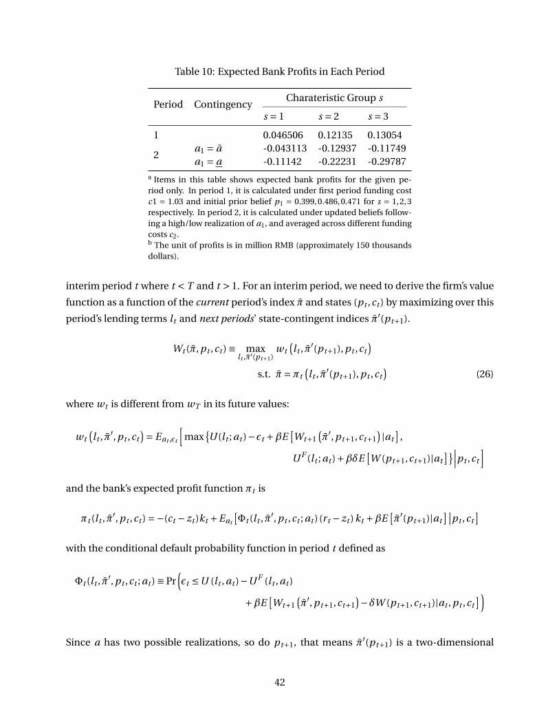
Table 10: Expected Bank Profits in Each Period

Period ContingencyCharateristic Group s

s = 1 s = 2 s = 3

1 0.046506 0.12135 0.13054

2a1 = a -0.043113 -0.12937 -0.11749a1 = a -0.11142 -0.22231 -0.29787

a Items in this table shows expected bank profits for the given pe-riod only. In period 1, it is calculated under first period funding costc1 = 1.03 and initial prior belief p1 = 0.399,0.486,0.471 for s = 1,2,3respectively. In period 2, it is calculated under updated beliefs follow-ing a high/low realization of a1, and averaged across different fundingcosts c2.b The unit of profits is in million RMB (approximately 150 thousandsdollars).

interim period t where t < T and t > 1. For an interim period, we need to derive the firm’s value

function as a function of the current period’s index π and states (pt ,ct ) by maximizing over this

period’s lending terms lt and next periods’ state-contingent indices π′(pt+1).

Wt (π, pt ,ct ) ≡ maxlt ,π′(pt+1)

wt(lt , π′(pt+1), pt ,ct

)s.t. π=πt

(lt , π′(pt+1), pt ,ct

)(26)

where wt is different from wT in its future values:

wt(lt , π′, pt ,ct

)= Eat ,εt

[max

{U (lt ; at )−εt +βE

[Wt+1

(π′, pt+1,ct+1

) |at]

,

U F (lt ; at )+βδE[W (pt+1,ct+1)|at

]}∣∣∣pt ,ct

]and the bank’s expected profit function πt is

πt (lt , π′, pt ,ct ) =−(ct − zt )kt +Eat

[Φt (lt , π′, pt ,ct ; at ) (rt − zt )kt +βE

[π′(pt+1)|at

]∣∣pt ,ct]

with the conditional default probability function in period t defined as

Φt (lt , π′, pt ,ct ; at ) ≡ Pr(εt ≤U (lt , at )−U F (lt , at )

+βE[Wt+1

(π′, pt+1,ct+1

)−δW (pt+1,ct+1)|at , pt ,ct])

Since a has two possible realizations, so do pt+1, that means π′(pt+1) is a two-dimensional

42

vector. In total there are five choice variables in this constrained optimization problem.

The first period’s problem is the same as in (21). In terms of solution method, I use backward

induction, starting from the last period. Using estimated parameters and firm’s value function

in the short-term model, I first calculate WT (·, ·, ·) from (22) under each combination of π, p

and c, where π, p are discretized on a grid and c takes four discrete values.37 I interpolate in

between grids of π to obtain the function WT (·, p,c) for each combination of p and c.38

For any t = T − 1, ...,1, given the function Wt+1(·, p,c), for any πt on the grid of π, any pt on

the grid of p and each of the four values of ct , I find the two possible next period belief pt+1

conditional on a high and low realization of at , denoted as p Ht+1 = pt+1

(pt |at = a

)and pL

t+1 =pt+1

(pt |at = a

). Then I plug functions Wt+1(·, p H

t+1,ct+1) and Wt+1(·, pLt+1,ct+1) into the period

t problem (26) where πt serves in the constraint. By solving this problem I obtain the optimal

first period lending terms lt , as well as indices π following a high and low realizations: π(p Ht+1)

and π(pLt+1). And I interpolate in between grids of π to obtain the function Wt (·, p,c).

I repeat the process above until I reach the first period. The only difference between t = 1 an

t > 1 is that I do not need to solve the first-period problem under various values of π1; instead,

the equilibrium condition imposes π1 = 0, i.e., the bank’s expected profit at the beginning of the

first period should be zero.

After getting the firm’s value function Wt (·, p,c) and the policy functions lt (·, ·, ·) and π′(·), I sim-

ulated a panel of lending terms, state variables, productivity realizations, and default outcomes,

for each firm in the observed data, where parameters are based on estimates of the baseline

model. The results shown in the next section are under T = 20. (But only the first seven year’s

statistics are shown because the baseline model is only seven period).

6.3 Simulation Results

Optimal Long-Term Contract

Optimal long-term contracts specify a schedule of future contract terms based on both the

length of the contractual relationship and performances in each year of the relationship. I later

refer to it as a relationship and performance-based schedule. It shows different dynamics than

the repeated short-term contracts. As a first pass, we can look at Table 11 which shows mean r ,

37The grid of p is the same as in baseline estimation, from 0 to 1 with step length 0.01. The grid of π is -1 to 1 withstep length 0.01, and this grid is large enough in the sense that chosen values of π in the equilibrium do not hit thebounds of the grid.

38I use cubic spline interpolation to ensure smoothness and facilitate the first-period maximization problem.

43

k, z and default rates from the baseline model and counterfactual model in each period, by dif-

ferent firm characteristic groups. Initial interest rates in the counterfactual long-term contract

are much higher than in the short-term contract, but later on interest rates in the long-term

contract drastically decline, and in most cases even lower than interest rates than the short-

term contract in the last several periods. This front-loading pricing scheme locks firms in by

charging high initial prices, and gradually let price go down (even lower than the spot-market

price) in later periods.

Why this front-loading pricing structure is optimal? This is because the promise of lower prices

in the future can incentivize firms to hold on and not default, which can alleviate agency friction

to some degree. The reduced agency friction also means less constrained capital input, i.e., loan

size in later periods of the long-term contracts are larger than the short-term contracts. Another

consequence of reduced agency friction is the less collateral coverage in long-term contracts,

which is beneficial to firms because it saves transaction costs associated with collateral. Overall

we see default rates in each single period go down, and lower defaults means more firms can

survive.

Long-term contracts also differ from repeated short-term contracts in the contractual response

to firm performances. Recall that in Table 5, the short-term contracts in the baseline model fea-

tures a jump in interest rates for firms whose performance is poor in the last period. Does the

optimal long-term contract still have this feature of raising prices following poor performance?

It turns out it is the opposite: the long-term contract actually specify a lower price if the firm

is hit by a negative productivity shock. We can see this from running the same regression as

in Equation (2), where I use firm fixed effect model to regress contract terms on years of re-

lationship t , indicator of poor performance in the previous period, Poor Rati ng t−1, and the

interaction term t ×Poor Rati ng t−1. I conduct this regression for firms who never had a single

poor performance in their history (in which case the variable Poor Per ft−1 and its interaction

term with t will be omitted, and we will only compare the rate of change of contract terms over

time), and for firms who have at least one poor performance in their history (again for these

firms I keep observation t <= t∗i +1 where t∗i is the first time firm i is rated poorly). Results are

shown in Table 12.

Comparing column (1) to (3) of Table 12 with column (1) to (3) of Table 5, we find that signs of

coefficients in the two tables are same, but the magnitudes of coefficients in the counterfactual

long-term contracts are much bigger, meaning that long-term contract has a more significant

time trend of declining lending spread and collateral coverage, and growing loan size. Focusing

on column (4), we find that coefficients of Poor Rati ng and the interaction term in the coun-

44

Table 11: Comparison of Long-Term Counterfactual Model vs. Short-Term Baseline Model byFirm Characteristics

Interest Rate Loan Size Collateral Coverage Default

Baseline C.F. Baseline C.F. Baseline C.F. Baseline C.F.

Characteristic Group s = 1

1 7.276 20.891 2.518 2.485 0.546 0.561 0.053 0.0432 7.105 18.885 2.529 2.511 0.545 0.421 0.053 0.0413 6.906 16.788 2.542 2.536 0.544 0.287 0.063 0.0484 6.775 14.483 2.550 2.558 0.544 0.160 0.055 0.0405 6.677 12.390 2.557 2.578 0.544 0.056 0.049 0.0376 6.622 9.997 2.561 2.611 0.543 0.000 0.061 0.0467 6.567 7.764 2.564 2.655 0.543 0.000 0.054 0.033

Characteristic Group s = 2

1 9.830 23.422 4.072 4.094 0.619 0.633 0.110 0.0882 9.647 19.872 4.090 4.157 0.618 0.548 0.136 0.1173 9.469 16.669 4.106 4.190 0.618 0.432 0.134 0.1024 9.325 13.605 4.120 4.216 0.617 0.332 0.111 0.0955 9.254 10.574 4.128 4.235 0.617 0.248 0.114 0.0866 9.188 6.782 4.134 4.248 0.617 0.179 0.101 0.0737 9.105 3.889 4.144 4.261 0.617 0.142 0.119 0.097

Characteristic Group s = 3

1 5.088 15.366 8.644 8.631 0.480 0.418 0.017 0.0132 4.882 12.650 8.688 8.677 0.479 0.299 0.013 0.0123 4.746 9.603 8.718 8.712 0.479 0.201 0.017 0.0154 4.602 6.358 8.748 8.746 0.478 0.133 0.012 0.0125 4.535 3.454 8.763 8.766 0.478 0.097 0.012 0.0116 4.482 3.270 8.774 8.777 0.478 0.096 0.018 0.0197 4.433 3.223 8.785 8.788 0.477 0.096 0.013 0.013

45

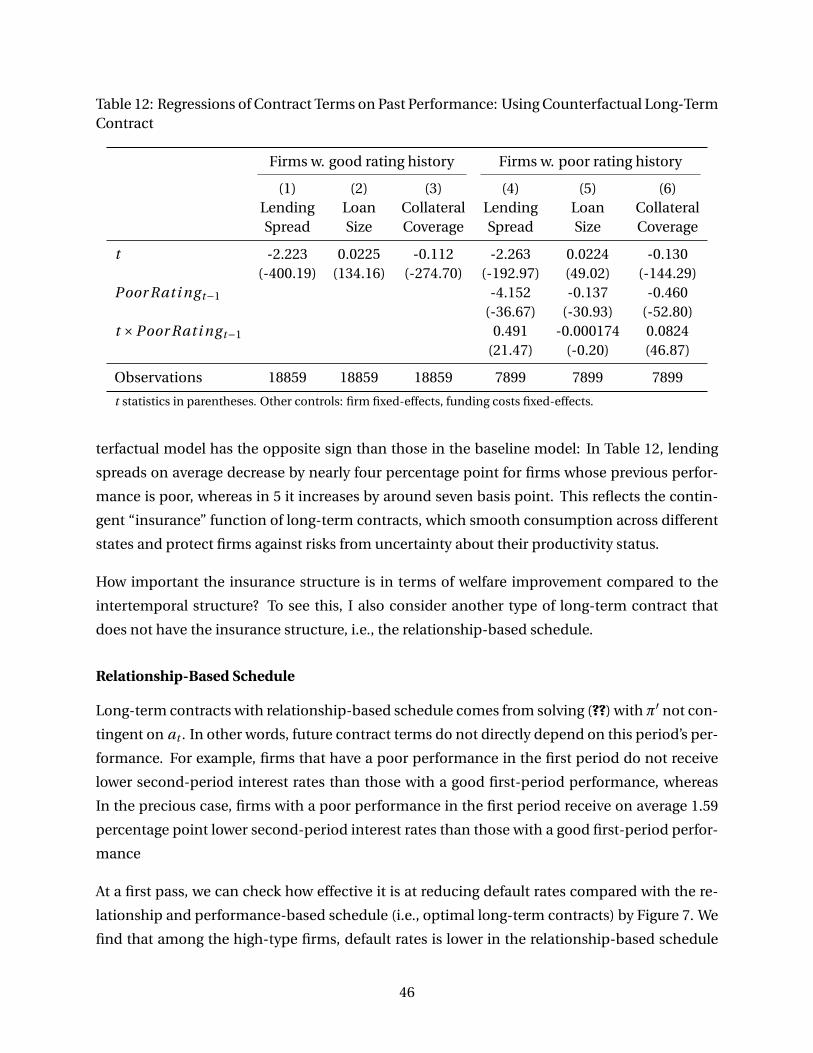
Table 12: Regressions of Contract Terms on Past Performance: Using Counterfactual Long-TermContract

Firms w. good rating history Firms w. poor rating history

(1)LendingSpread

(2)LoanSize

(3)CollateralCoverage

(4)LendingSpread

(5)LoanSize

(6)CollateralCoverage

t -2.223 0.0225 -0.112 -2.263 0.0224 -0.130(-400.19) (134.16) (-274.70) (-192.97) (49.02) (-144.29)

Poor Rati ng t−1 -4.152 -0.137 -0.460(-36.67) (-30.93) (-52.80)

t ×Poor Rati ng t−1 0.491 -0.000174 0.0824(21.47) (-0.20) (46.87)

Observations 18859 18859 18859 7899 7899 7899

t statistics in parentheses. Other controls: firm fixed-effects, funding costs fixed-effects.

terfactual model has the opposite sign than those in the baseline model: In Table 12, lending

spreads on average decrease by nearly four percentage point for firms whose previous perfor-

mance is poor, whereas in 5 it increases by around seven basis point. This reflects the contin-

gent “insurance” function of long-term contracts, which smooth consumption across different

states and protect firms against risks from uncertainty about their productivity status.

How important the insurance structure is in terms of welfare improvement compared to the

intertemporal structure? To see this, I also consider another type of long-term contract that

does not have the insurance structure, i.e., the relationship-based schedule.

Relationship-Based Schedule

Long-term contracts with relationship-based schedule comes from solving (??) with π′ not con-

tingent on at . In other words, future contract terms do not directly depend on this period’s per-

formance. For example, firms that have a poor performance in the first period do not receive

lower second-period interest rates than those with a good first-period performance, whereas

In the precious case, firms with a poor performance in the first period receive on average 1.59

percentage point lower second-period interest rates than those with a good first-period perfor-

mance

At a first pass, we can check how effective it is at reducing default rates compared with the re-

lationship and performance-based schedule (i.e., optimal long-term contracts) by Figure 7. We

find that among the high-type firms, default rates is lower in the relationship-based schedule

46

than in the relationship and performance-based schedule, whereas for low-type firms, default

rates is lower in the relationship and performance-based schedule than in the relationship-

based schedule. This is because the relationship and performance-based schedule provides

price discounts for firms with poor performance, which are more likely to be the low-type

firms, and such price discounts lead to lower default rates. Essentially the relationship and

performance-based schedule is employing a transfer from high-type to low-type.

To see the overall welfare implications of the two schedules, I calculate the associated cumu-

lative default probability over the seven-year period, total amount of capital and output taken

over the seven-year period, the firm size measured by output in the last period, and the initial

firm value in the baseline model with short-term contract, counterfactual model with relationship-

based long-term contract, and counterfactual model with relationship and performance-based

long-term contract. Summary of these statistics by firm quality type is show in Table 13.

Comparing column (3) with column (1), we find that with long-term contracts with fully flexi-

ble schedule, cumulative default probability over the seven-year period drops by 17.15%, with

high-type firm’s cumulative default probability drops by 16.86% and low-type 17.41%. Total

firm outputs over the seven-year period increases by 2.63%, where high-type firm’s total output

increases by 2.84% (due to a 2.88% increase in total capital input), and low-type firm’s total out-

puts increase by 2.45% (due to a 2.58% increase in total capital input). Comparing column (2)

with column (3), we find that the relationship-based schedule does a good job of capturing the

vast majority of the efficiency improvement without using complex contingency contracting.

47

Table 13: Comparison Across Different Contracts

Scenario

Baseline Counterfactual Long-Term Contracts

(1) (2) (3)

Short-Term Relationship-BasedRelationship and

Performance-Based

High-Type Firms

Cumulative Default Prob. .3325114 .2736879 .2765058

Total Capital 30.71789 31.64557 31.62901

Total Output 55.4055 57.00239 56.97651

Final Size 5.071709 5.130478 5.128197

Firm Value 86.39585 86.72219 86.7231

Low-Type Firms

Cumulative Default Prob. .3117363 .2585962 .2574595

Total Capital 29.27848 30.05414 30.03602

Total Output 51.87864 53.19209 53.15497

Final Size 4.751198 4.806808 4.809732

Firm Value 84.25609 84.58102 84.58202

All Firms

Cumulative Default Prob. .3210129 .265335 .2659641

Total Capital 29.92121 30.76476 30.74733

Total Output 53.45347 54.89348 54.86138

Final Size 4.894314 4.951335 4.951934

Firm Value 85.21154 85.5371 85.53806

I compare firm welfare in model with long-term contract with fully flexible schedules with the

efficient benchmark (with no agency friction and full information, as in column (1) of Table 6),

and I find that long-term contracts recover 31.46% of total welfare loss from both sources of

inefficiency (i.e., agency friction and incomplete information). And the average Compensating

Variation (CV) across firms is around $92,106.

48

7 Conclusion

Studies that focus on US commercial loan market highlight the long-term contractual rela-

tionships between firms and banks. However, in developing countries with relatively under-

developed financial market, long-term contracting can be too costly to implement. So how

much do firms in those markets miss out because of a lack of long-term contracting? This is the

question that this paper aims to answer.

This paper utilizes data from a Chinese bank where long-term contracting is hard to access, and

document several stylized facts in this novel dataset. I find that observed contracts are short-

term, with banks and firms negotiating contract terms on a annual basis. I find evidence of

learning by examining the dynamics of contract terms, the contractual response to measures of

firm performance, and how these responses change over time.

This paper provides a framework to analyze welfare impacts of contract structure. I develop a

dynamic model of lending markets to analysis bank’s choice of contract terms and firm’s choice

of repay or default. Inspired by features in the data, I assume that banks are unable to commit

to long-term financing contracts and can only offer short-term contracts, and that firms are

heterogeneous in unobserved types, with types unknown to banks and firms in the beginning

but can be learned over time. I estimate the model using the panel data, and identification

comes mainly from the over-time variations of contract terms and the its correlation with firm

performance and funding costs.

In the model there are two sources of inefficiency: agency friction (i.e., repayment behavior

cannot be enforced by contracts) and incomplete information (i.e., firm’s quality is unknown

in the beginning). Estimates show that agency friction is the more important source of ineffi-

ciency in this market. By conducting counterfactual analysis of enabling banks to commit to

long-term contracts, I find that long-term contracting can effectively alleviate agency friction

through its use of both intertemporal structure and intratemporal structure. The intertempo-

ral structure front-loads prices, which allows contract terms become increasingly favorable to

firms over time and thus disincentivize firm defaults. The intratemporal structure is like an in-

surance, protecting firms against risks of negative productivity shocks. I find that the majority

of welfare improvement comes from the intertemporal structure of long-term contracts, and

a long-term contract with only relationship-based schedule is almost as effective as the more

complex schedule that are contingent on performance history.

The main contribution of this paper is two fold. First, this paper provides an empirical frame-

work for the corporate lending market that incorporate both observed and unobserved firm

49

heterogeneity. Compared to previous models in macro-finance literature, my model can ac-

commodate assumptions on different contract structures, and utilize collateral information,

firm performance and loan outcome data to form a more accurate estimate on the level of

agency frictions in place. Second, this paper quantifies the value of long-term contracting for

small and medium-sized young firms in China. There has long been discussion about long-

term financing support for small and medium-sized firms in China, and this paper can provide

a measure of potential benefits that long-term financing arrangement can bring about.

The model can also be used for various policy experiments. For example, we can calculate how

does a reduction in bank’s funding costs translate into changes in interest rates, loan size, and

collateral coverage, and the associated default rates. As another example, we can simulate how

does a loan guarantee program (like Small Business Administration in US) change interest rates,

loan size and the associated default rates. We can further compare the effectiveness of different

policy interventions in terms of default prevention and enhancement in capital flow.

The model can be extended in the following aspects: (1) Learning by doing. We can allow

firms to “learn” through past production, i.e., more capital taken in the past can lead to higher

productivity on average. Then part of the observed growth in capital could be attributed to

learning-by-doing (In fact, observed capital growth is larger than the predicted capital growth

from the current model, and the unexplained part can be accounted for by a learning-by-doing

process). This can still be identified because we do see the firm performance history, which pins

down the belief updating process. So capital growth that cannot be explained by the belief up-

dating process will identify the learning-by-doing process. This is similar to the identification

argument in Pastorino (2019). (2) Aggregate productivity shocks. In the current model firm’s

productivity shocks are i.i.d. However it is possible that macro-economic conditions can cause

firm’s productivity realizations to be correlated (say firms within the same industry have cor-

relations in their productivity). It is possible to allow correlation structures among firms with

similar observed characteristics.

The model is better suited to study young firms, since I abstract away from asymmetric infor-

mation, which could be a more severe issue in establish firms. Another limitation is that model

does not take into account ex ante model hazard problem, where firms choose “effort” levels

in the beginning of each period that are unobserved by banks but could affect payoffs. In this

case the insurance-like structure of the long-term contract with relationship and performance-

based schedule might be problematic, but the relationship-based schedule can still use in-

tertemporal pricing structure as an incentive devise.

50

References

D. A. Ackerberg. Advertising, learning, and consumer choice in experience good markets: an

empirical examination. International Economic Review, 44(3):1007–1040, 2003.

W. Adams, L. Einav, and J. Levin. Liquidity constraints and imperfect information in subprime

lending. American Economic Review, 99(1):49–84, 2009.

R. Albuquerque and H. A. Hopenhayn. Optimal lending contracts and firm dynamics. The

Review of Economic Studies, 71(2):285–315, 2004.

C. Arellano, Y. Bai, and J. Zhang. Firm dynamics and financial development. Journal of Monetary

Economics, 59(6):533–549, 2012.

P. Asquith, A. Beatty, and J. Weber. Performance pricing in bank debt contracts. Journal of

Accounting and Economics, 40(1-3):101–128, 2005.

J. P. Atal. Lock-in in dynamic health insurance contracts: Evidence from chile. PIER Working

Paper No. 5694, 2019.

T. Berg, A. Saunders, and S. Steffen. The total cost of corporate borrowing in the loan market:

Don’t ignore the fees. The Journal of Finance, 71(3):1357–1392, 2016.

B. Biais, T. Mariotti, J.-C. Rochet, and S. Villeneuve. Large risks, limited liability, and dynamic

moral hazard. Econometrica, 78(1):73–118, 2010.

Y. Boualam. Credit markets and relationship capital. Working paper, University of North Car-

olina, 2018.

F. J. Buera, J. P. Kaboski, and Y. Shin. Finance and development: A tale of two sectors. American

Economic Review, 101(5):1964–2002, 2011.

F. J. Buera, J. P. Kaboski, and Y. Shin. Entrepreneurship and financial frictions: A macrodevelop-

ment perspective. Annual Review of Economics, 7(1):409–436, 2015.

Y.-S. Chan and G. Kanatas. Asymmetric valuations and the role of collateral in loan agreements.

Journal of money, credit and banking, 17(1):84–95, 1985.

G. L. Clementi and H. A. Hopenhayn. A theory of financing constraints and firm dynamics. The

Quarterly Journal of Economics, 121(1):229–265, 2006.

J. H. Cochrane. Time-consistent health insurance. Journal of Political Economy, 103(3):445–473,

51

1995.

T. F. Cooley and V. Quadrini. Financial markets and firm dynamics. American economic review,

91(5):1286–1310, 2001.

B. G. S. Crawford, N. Pavanini, and F. Schivardi. Asymmetric Information and Imperfect Com-

petition in Lending Markets. 108(7):1659–1701, 2018.

G. S. Crawford and M. Shum. Uncertainty and learning in pharmaceutical demand. economet-

rica, 73(4):1137–1173, 2005.

P. M. DeMarzo and M. J. Fishman. Optimal long-term financial contracting. The Review of

Financial Studies, 20(6):2079–2128, 2007.

P. M. DeMarzo and Y. Sannikov. Optimal security design and dynamic capital structure in a

continuous-time agency model. The Journal of Finance, 61(6):2681–2724, 2006.

L. Einav, M. Jenkins, and J. Levin. Contract pricing in consumer credit markets. Econometrica,

80(4):1387–1432, 2012.

H. Gao, H. Ru, R. M. Townsend, and X. Yang. Rise of bank competition: Evidence from banking

deregulation in china. NBER working paper, (w25795), 2019a.

H. Gao, H. Ru, and X. Yang. What do a billion observations say about distance and relationship

lending? Available at SSRN 3195616, 2019b.

M. Gertler. Financial capacity and output fluctuations in an economy with multi-period finan-

cial relationships. The Review of Economic Studies, 59(3):455–472, 1992.

D. He and H. Wang. Dual-track interest rates and the conduct of monetary policy in china.

China Economic Review, 23(4):928–947, 2012.

I. Hendel and A. Lizzeri. The role of commitment in dynamic contracts: Evidence from life

insurance. The Quarterly Journal of Economics, 118(1):299–328, 2003.

C.-T. Hsieh and P. J. Klenow. Misallocation and manufacturing tfp in china and india. The

Quarterly journal of economics, 124(4):1403–1448, 2009.

C.-T. Hsieh and P. J. Klenow. The life cycle of plants in india and mexico. The Quarterly Journal

of Economics, 129(3):1035–1084, 2014.

K. P. Huynh and R. J. Petrunia. Age effects, leverage and firm growth. Journal of Economic

52

Dynamics and Control, 34(5):1003–1013, 2010.

R. G. King and R. Levine. Finance, entrepreneurship and growth. Journal of Monetary eco-

nomics, 32(3):513–542, 1993.

J. Li and X. Lin. Assessing credit guarantee companies in china: Applying a new framework.

China Economic Review, 44:98–111, 2017.

M. Manove, A. J. Padilla, and M. Pagano. Collateral versus project screening: A model of lazy

banks. Rand journal of economics, pages 726–744, 2001.

G. Manso, B. Strulovici, and A. Tchistyi. Performance-sensitive debt. The Review of Financial

Studies, 23(5):1819–1854, 2010.

M. McMahon, M. A. Schipke, and X. Li. China’s monetary policy communication: Frameworks,

impact, and recommendations. International Monetary Fund, 2018.

V. Midrigan and D. Y. Xu. Finance and misallocation: Evidence from plant-level data. American

economic review, 104(2):422–58, 2014.

K. Okazaki. Banking system reform in china: The challenges of moving toward a market-

oriented economy. Technical report, Rand Corp Arlington Va National Security Research Div,

2007.

E. Pastorino. Careers in firms: the role of learning and human capital. Technical report, Tech-

nical report, mimeo, 2019.

N. Porter, E. Takáts, and T. Feyzioglu. Interest rate liberalization in china. IMF Working Papers,

pages 1–28, 2009.

V. Quadrini. Investment and liquidation in renegotiation-proof contracts with moral hazard.

Journal of Monetary Economics, 51(4):713–751, 2004.

S. A. Sharpe. Credit rationing, concessionary lending, and debt maturity. Journal of Banking &

Finance, 15(3):581–604, 1991.

J. Thomas and T. Worrall. Foreign direct investment and the risk of expropriation. The Review

of Economic Studies, 61(1):81–108, 1994.

Y. Xin. Asymmetric information, reputation, and welfare in online credit markets. Available at

SSRN 3580468, 2020.

53

B. Xu, A. van Rixtel, and M. Van Leuvensteijn. Measuring bank competition under binding in-

terest rate regulation: the case of china. Applied Economics, 48(49):4699–4718, 2016.

54

8 Additional Tables

Table 14: Summary Statistics

Year in

Relationship t

Interest

Rate r

Loan Size

k

Collateral

Coverage zPoorRating Default

1 7.043 4.482 0.573 0.081 0.040

2 7.051 5.009 0.573 0.085 0.066

3 6.826 5.371 0.570 0.084 0.081

4 6.577 5.839 0.568 0.082 0.051

5 6.420 6.485 0.565 0.089 0.079

6 6.165 7.120 0.560 0.083 0.050

7 6.004 7.572 0.535 0.089 0.080

Average 6.863 5.195 0.567 0.085 0.058

Table 15: Moment Restrictions

Meaning Moment Restrictions Dimension

Decisions on contract term and default E{i }[Oi −Oi |Xi

]21×28

Firm performances E{i }[Pi − Pi |Xi

]21×7

Covariance between firm performance and decisions E{i }[Pi Oi − Pi Oi |Xi

]21×28

Covariance between cost of fund and decisions E{i }[Ci Oi − Ci Oi |Xi

]21×28

55

9 Additional Graphs

Figure 2: Distribution of Relationship Duration

56

(a) Residualized Lending Spread

(b) Residualized Loan Size

(c) Residualized Collateral Coverage

Figure 3: Time Profile of Residualized Contract Terms

57

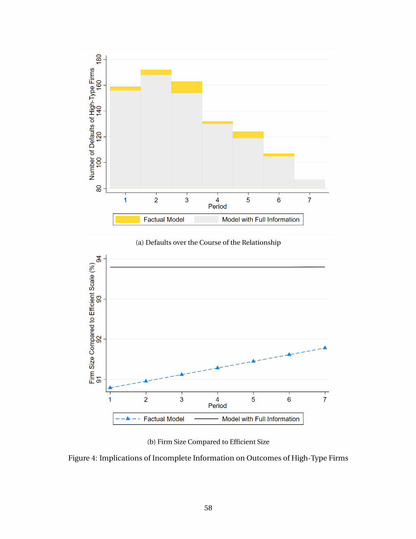
(a) Defaults over the Course of the Relationship

(b) Firm Size Compared to Efficient Size

Figure 4: Implications of Incomplete Information on Outcomes of High-Type Firms

58

(a) Mispricing in the First Period (b) Mispricing in the Last Period

Figure 5: Mispricing over the Course of the Relationship

(a) Misallocation of Capital in the First Period (b) Misallocation of Capital in the Last Period

Figure 6: Misallocation of Capital over the Course of the Relationship

59

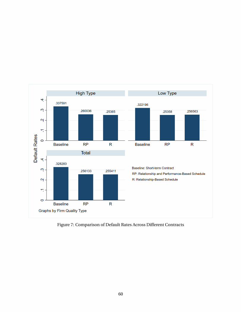
Figure 7: Comparison of Default Rates Across Different Contracts

60