1 The role of instability waves in predicting jet noise M.E. Goldstein National Aeronautics and Space Administration Glenn Research Center Cleveland, Ohio 44135 S.J. Leib Ohio Aerospace Institute Brook Park, Ohio 44142 There has been an ongoing debate about the role of linear instability waves in the prediction of jet noise. Parallel mean flow models, such as the one proposed by Lilley, usually neglect these waves because they cause the solution to become infinite. The resulting solution is then non-causal and can, therefore, be quite different from the true causal solution for the chaotic flows being considered here. The present paper solves the relevant acoustic equations for a non-parallel mean flow by using a vector Green’s function approach and assuming the mean flow to be weakly non-parallel, i.e., assuming the spread rate to be small. It demonstrates that linear instability waves must be accounted for in order to construct a proper causal solution to the jet noise problem. . Recent experimental results (e.g., see Tam, Golebiowski, and Seiner,1996) show that the small angle spectra radiated by supersonic jets are quite different from those radiated at larger angles (say, at 90 o ) and even exhibit dissimilar frequency scalings (i.e., they scale with Helmholtz number as opposed to Strouhal number). The present solution is (among other things )able to explain this rather puzzling experimental result. _____________________________________________________________________________________________ 1. Introduction Lighthill (1952, 1954) provided a systematic basis for predicting jet noise when he rearranged the Navier- Stokes equations into the form of a linear wave equation for a medium at rest with a quadrupole-type source term (which includes a pressure/density contribution that Lilley (1974) showed to be more appropriately described by a dipole-type source.) The crucial step in this so-called acoustic analogy approach amounts to assuming that the https://ntrs.nasa.gov/search.jsp?R=20050198898 2018-06-20T03:28:34+00:00Z

Welcome message from author
This document is posted to help you gain knowledge. Please leave a comment to let me know what you think about it! Share it to your friends and learn new things together.
Transcript
1
The role of instability waves in predicting jet noise
M.E. Goldstein
National Aeronautics and Space Administration
Glenn Research Center
Cleveland, Ohio 44135
S.J. Leib
Ohio Aerospace Institute
Brook Park, Ohio 44142
There has been an ongoing debate about the role of linear instability waves in the prediction of jet noise.
Parallel mean flow models, such as the one proposed by Lilley, usually neglect these waves because they cause the
solution to become infinite. The resulting solution is then non-causal and can, therefore, be quite different from the
true causal solution for the chaotic flows being considered here. The present paper solves the relevant acoustic
equations for a non-parallel mean flow by using a vector Green’s function approach and assuming the mean flow to
be weakly non-parallel, i.e., assuming the spread rate to be small. It demonstrates that linear instability waves must
be accounted for in order to construct a proper causal solution to the jet noise problem. . Recent experimental results
(e.g., see Tam, Golebiowski, and Seiner,1996) show that the small angle spectra radiated by supersonic jets are quite
different from those radiated at larger angles (say, at 90o) and even exhibit dissimilar frequency scalings (i.e., they
scale with Helmholtz number as opposed to Strouhal number). The present solution is (among other things )able to
explain this rather puzzling experimental result.
_____________________________________________________________________________________________
1. Introduction
Lighthill (1952, 1954) provided a systematic basis for predicting jet noise when he rearranged the Navier-
Stokes equations into the form of a linear wave equation for a medium at rest with a quadrupole-type source term
(which includes a pressure/density contribution that Lilley (1974) showed to be more appropriately described by a
dipole-type source.) The crucial step in this so-called acoustic analogy approach amounts to assuming that the
https://ntrs.nasa.gov/search.jsp?R=20050198898 2018-06-20T03:28:34+00:00Z
2
source term is in some sense known or that it can at least be modeled in an approximate fashion. Early efforts to
improve the Lighthill approach focused on accounting for mean flow interaction effects. Phillips (1960), Lilley
(1974), and many others, sought to accomplish this by rearranging the Navier-Stokes equations into the form of an
inhomogeneous convective, or moving medium, wave equation rather than the inhomogeneous stationary medium
wave equation originally proposed by Lighthill. Current industrial noise prediction methods, such as GE’s MGB
approach (Balsa et al. 1978), are based on a form of the convective wave equation proposed by Lilley (1974) in
which the wave operator is appropriate to sound propagation on a parallel mean flow and therefore possesses
homogeneous solutions corresponding to spatially growing instability waves on that flow (Betchov and Criminale,
1967).
The complete solution to this equation consists of a particular solution plus these homogeneous contributions,
but the result cannot be used to calculate the far-field noise because the instability waves become unbounded
(infinite) far downstream in the flow . The usual resolution to this dilemma is to completely neglect the contribution
of the instability waves. Unfortunately, the resulting solution turns out to be non-causal, which may be particularly
serious in flows that support instabilities (i.e., chaotic flows) because small changes in initial (and/or boundary)
conditions can produce large (i.e., O(1)) changes in the steady state solution. Arguments against imposing a
causality requirement (Mani, 1976; Dowling, et. al. 1978 ) usually amount to asserting that it is unnecessary
because it is not possible to identify an initial time before which the fluctuations (about the base flow) have been
“switched on’ in an acoustic analogy approach and that a boundedness requirement can, therefore, be imposed on
the solution.
A better approach might be to begin with an equation appropriate to sound propagation on a non-parallel flow,
say the actual mean flow in the jet. The most important difference between this approach and Lilley’s parallel flow
result is that the homogeneous solutions to the acoustic equations correspond to instability waves that grow and then
decay on the diverging, non-parallel base flow and therefore always remain bounded—which eliminates the
dilemma alluded to above. But since the homogeneous solutions are now bounded, this leaves the mathematical
problem incompletely specified (i.e., ill posed) and the imposition of causality appears to be the most reasonable
way of making the solution unique in this case. Our view is that the causality amounts to more than just imposing
appropriate initial conditions and that it serves ( as demonstrated at the end of section 4) to insure the appropriate
3
cause- effect relation between the sound and its turbulent source when it is imposed on the Green’s function, as is
done below.
The present paper develops a causal solution to the relevant acoustic equations by using a vector Green’s
function approach and assuming that the mean flow spread rate, say ε, is small. This implies that all streamwise
changes in that flow occur on the slow streamwise length scale εx1, where x1 is the (suitably normalized) coordinate
in the flow direction. The appropriate casual Green’s function consists of a component that decays to zero when the
unscaled streamwise coordinate x1 – x1′ becomes large (where x1′ corresponds to the source location) plus a
component that becomes unbounded when the unscaled streamwise coordinate becomes large but decays to zero on
the long (slow) streamwise length scale ε (x1 – x1′). The former component can be calculated by treating the slow
variable εx1 as a parameter and using the locally parallel flow approximation to simplify the results.
This approximation cannot, however, be used to determine the latter component (which corresponds to a
superposition of linear instability waves; Briggs, 1964; Bers, 1975), since the resulting local solution would become
unbounded and would not remain valid over the long streamwise length scale ε (x1 – x1′) on which this component
evolves. The appropriate result is obtained by retaining O(ε) terms in the Green’s function equations and using the
method of multiple scales, the WKBJ method and matched asymptotic expansions to render the solution uniformly
valid.
Both components of the Green’s function act on the same source term and each is capable of producing acoustic
radiation—even at subsonic Mach numbers. The first corresponds to the usual Lilley equation solution, but with
slowly varying coefficients and with slightly modified source terms. The second is associated with linear instability
waves, but is very different from conventional instability models since these waves are now continuously
“generated” along the length of the jet and do not constitute separate sound sources. Their only role is to produce the
appropriate Green’s function, and they may not even correspond to actual physical flow structures. Mani’s (1976)
assertion that the instability waves generate the turbulence and should, therefore, be excluded is irrelevant here
because their inclusion in the Green’s function only serves to produce the appropriate cause-effect relation between
the sound and its turbulent source and, therefore, corresponds to a different aspect of their behavior.
Each component of this function can be thought of as a filter that only allows certain elements of the source
spectrum to reach the far field. The resulting acoustic spectrum is expected to exhibit a bi-model structure because
the second Green’s function component only responds to frequencies in the range where the instabilities exhibit
4
spatial growth, which is somewhat lower than the frequency range selected by the first term. Preliminary
calculations for a two dimensional mixing layer (Goldstein & Handler, 2003 ) suggest that the contribution of the
second Green’s function component will be fairly small at subsonic Mach numbers, but that it should be quite large
at supersonic speeds and dominate the first term at small angles to the downstream jet axis. Recent experimental
results (e.g., see Tam, Golebiowski, and Seiner,1996) show that the small angle spectra radiated by supersonic jets
are quite different from those radiated at larger angles (say, at 90o) and even exhibit dissimilar frequency scalings
(i.e., they scale with Helmholtz number as opposed to Strouhal number). Until now this curious behavior seems to
have defied explanation, but our model calculations show that it can be attributed to the fact that each of these
Green’s function components is the dominant carrier of the acoustic radiation at different angles to the jet axis. As
noted above, the large differences between the present result and the usual non-causal Lilley’s equation solutions are
directly related to the chaotic nature of the flow.
The fundamental acoustic equations, which we refer to as the LNS equations, are introduced in section 2 and the
Lilley’s equation as well as the equations for a steady but nonparallel base flow (i.e., the actual time- average flow)
are obtained as special cases in section 3. A formal vector Green’s function solution to the general LNS equations is
given in section 4 and a local causal, small- ε asymptotic approximation to this solution is constructed in section 5.
The corresponding uniformly valid solution is obtained in section 6, and its far field expansion is worked out in
section 7. This result is then used to derive an expression for the far field acoustic spectrum in section 8. The
general formulas are applied to a round jet in section 9 and some simplifying approximations are introduced in
section 10. Section 11 contains some qualitative comparisons between the numerical computations based on this
simplified model and the available experimental data.
2. The Fundamental Equations
Goldstein (2002, hereafter referred to as I) showed that the Navier-Stokes equations,
0,jjt xν ν
∂ ∂Λ + Γ =
∂ ∂ (2.1)
where the summation convention is being used, but with the Greek indices ranging from 1 to 5 (to represent the five
first order equations), while the Latin indices i, j are restricted to the range 1,2,3, { } { }, ,i ov h pνΛ = ρ ρ − ρ ,
{ } { }, ,j i j ij ij j o j i ij jv v p v h q v vνΓ = ρ + δ − σ ρ + − σ ρ ,
5
212oh h v≡ + (2.2)
denotes the stagnation enthalpy, h denotes the enthalpy, t denotes the time, x ≡ {x1,x2,x3} are Cartesian coordinates,
p denotes the pressure, ρ denotes the density, v = {v1,v2,v3} is the fluid velocity, σij is the viscous stress tensor, qi is
the heat flux vector, { }, ,i ov h pρ ρ − ρ is shorthand for { }1 2 3, , , ,ov v v h pρ ρ ρ ρ − ρ etc., and the dependent variables are
assumed to satisfy the ideal gas law:
, ,pp RT h c T=ρ = (2.3)
with R = cp − cv being the gas constant, cp and cv are the specific heats at constant pressure and volume, respectively,
and T the absolute temperature, can be recast into the form of the linearized Navier-Stokes equations by dividing the
dependent variables
, , , ,i i ip p p h h h v v v′ ′ ′ ′ρ = ρ + ρ = + = + = +% % (2.4)
as well as the viscous stressσij and heat flux qi, into their ‘base flow’ components , , , , , and ,i ij ip h v qρ σ% % and into
their ‘residual’ components , , , , , and ,i ij ip h v q′ ′ ′ ′ ′ ′ρ σ and requiring that the former satisfy the inhomogeneous
Navier−Stokes equations
0,jjt xν ν
∂ ∂Λ + Γ =
∂ ∂% % (2.5)
along with an ideal gas law equation of state,
,pp
c ph c TR
= =ρ
% % (2.6)
6
where{ } { }, ,i o ov h p HνΛ = ρ ρ − − ρ%% %% ,{ } { }, ,j i j ij ij ij j o j i ij j j o jv v p T v h q v H v H vνΓ = ρ + δ − σ − ρ + − σ − − ρ%% % %% % % % % % %
21
2oh h v≡ +% % % (2.7)
is the base flow stagnation enthalpy, and the ‘sources strengths’ , , and ij o jT H H% % % , which are assumed to be localized,
can otherwise be specified arbitrarily.
The residual variables are governed by the Linearized Navier-Stokes (LNS) equations
,v vL u sµ µ= (2.8)
where
{ } { }, ,v i ou u p′ ′ ′≡ ρ ρ , (2.9)
with
i iu v′ ′ρ ≡ ρ (2.10)
and
( ) 2112o op p v H⎛ ⎞′ ′ ′≡ + γ − ρ +⎜ ⎟
⎝ ⎠% , (2.11)
is a five dimensional (non-linear) dependent variable vector,
( )24 4 5 ,v v o v v vL D c Kµ µ µ µ µ µ≡ δ + δ ∂ + ∂ δ + δ + (2.12)
with
( )5 4 41 11 ,j j vj
v v v vj j j
vK v
x x xµ
µ µ µ
⎛ ⎞∂τ ∂ ∂τ≡ ∂ − δ + γ − δ − δ⎜ ⎟⎜ ⎟ρ ∂ ∂ ρ ∂⎝ ⎠
% % %% (2.13)
7
,ij ij ij ijp Tτ ≡ δ − − σ%% (2.14)
, 1,2,3
ii
xµ∂
∂ ≡ = µ =∂
, (2.15)
oD denotes the linear operator
o jj
D vt x
∂ ∂≡ +
∂ ∂% , (2.16)
.
and µ∂ , vµ% , µjτ% all equal to zero when µ > 3, is the 5-dimensional linear Euler operator. The 5-dimensional source
vector sµ is given by
( )4 1 ,ij ij
j j
vs e e
x xµ µ µ∂∂ ′ ′≡ + δ γ −
∂ ∂% (2.17)
where γ ≡ cp/cv is the specific heat ratio, the source strengths ie ν′ are given by
( )2
1 ,2i i i i o ive v v T Hν ν ν ν ν
⎛ ⎞′ρ′ ′ ′ ′≡ −ρ − + δ γ − + + σ⎜ ⎟⎜ ⎟⎝ ⎠
% % (2.18)
for 1,2.., 4ν = and zero otherwise and we have put
( ) ( )12 2 24 2
112
v h v c vγ−⎛ ⎞ ′′ ′ ′ ′≡ γ − + = +⎜ ⎟⎝ ⎠
(2.19)
( )( )4 1i i ij jT H T v= γ − −% % % % (2.20)
and
( )( )4 1 .j j jl lq v′ ′ ′σ = − γ − − σ (2.21)
8
Equations (2.9) are easily converted into the usual convective form of the LNS equations by using the 5th component
of the base flow equation (2.5) to show that
o jj
D f v ft x
⎛ ⎞∂ ∂ρ = ρ +⎜ ⎟⎜ ⎟∂ ∂⎝ ⎠
% . (2.22)
They are written out in the more familiar, but less compact, vector form in I.
3. Lilley’s Equation and the Non-Parallel Mean Flow Result
The base flow equations (2.5) reduce to the usual Euler equations when the arbitrary source strengths
, , and ij j oT H H% % % , and the mean viscous stress and heat fluxij iqσ are set equal to zero. A general class of solutions
to these equations, which quite conveniently provides a good approximation to the actual mean flow field in a jet, is
the unidirectional transversely sheared mean flow
( ) ( )1 2 3 2 3, , constant, , .i iv U x x p x x= δ = ρ = ρ% (3.1)
The 5th component of the LNS equation then decouples from the remaining four components, which now
become the inhomogeneous compressible Rayleigh equations (Betchov and Criminale 1967)
1o i o
i j ijj i j
D u pUu eDt x x x
⎛ ⎞′ ′∂∂ ∂′ ′ρ + δ + =⎜ ⎟⎜ ⎟∂ ∂ ∂⎝ ⎠ (3.2)
( )411j jo o
jj j j
u eD p Up eDt x x x
′ ′∂ ∂′ ∂′+ γ = + γ −∂ ∂ ∂
(3.3)
where Do/Dt reduces to the usual convective derivative
1
oDU
Dt t x∂ ∂
= +∂ ∂
. (3.4)
9
It is now well known (see chapter 1 of Goldstein 1976), that the velocity-like variable ′ui can be eliminated between
these equations (by taking the divergence of the first equation and the convective derivative of the second,
subtracting the results and then using the first equation to eliminate the velocity fluctuation on the left-hand side) to
obtain the inhomogeneous Pridmore−Brown (1958 ) equation
( )2 2
42 212
12 1ij ij jo o
o ji j i j j j
e e eD DU ULp c c eDt x x x x x x xDt
′ ′ ′⎛ ⎞ ⎡ ⎤∂ ∂ ∂∂ ∂ ∂′ ′= − − + γ −⎜ ⎟ ⎢ ⎥⎜ ⎟∂ ∂ ∂ ∂ ∂ ∂ ∂⎢ ⎥⎝ ⎠ ⎣ ⎦ (3.5)
where
2
2 22
12o o
i i j j
D D UL c cDt x x x x xDt
⎛ ⎞∂ ∂ ∂ ∂ ∂≡ − −⎜ ⎟⎜ ⎟∂ ∂ ∂ ∂ ∂⎝ ⎠
(3.6)
is the variable-density Pridmore−Brown (1958) operator, and
( )2
2 3,c p x x= γ ρ (3.7)
is the square of the mean flow sound speed.
This is a form of Lilley’s equation that was derived in I. As noted in the Introduction, it possesses homogeneous
solutions corresponding to spatially growing instability waves on the base flow (3.1) (Betchov and Criminale, 1967).
It also possesses homogeneous solutions corresponding to the continuous spectrum. The complete solution to this
equation consists of a particular solution plus these homogeneous contributions, but the result is meaningless
because the instability waves become unbounded (infinite) far downstream in the flow. The usual resolution to this
dilemma is to completely neglect the instability wave contribution. Unfortunately, this causes the solution to be non-
causal which, as noted in the introduction, can lead to erroneous results.
A better resolution is obtained by choosing the base flow in (2.8) to be the actual mean flow of the jet. The over
bars on the dependent base flow variables then denote the time average
( )1lim ,2
T
TT
t dtT→∞
−
• ≡ •∫ x (3.8)
10
where the dot is a place holder for ρ, vi, p, and h, and
( )• ≡ ρ • ρ% (3.9)
denotes a Favre (1969) averaged quantity for all variables except ~ho , which is defined by (2.7). Notice that (2.6) is
completely consistent with the overall ideal gas law (2.3) when the tilde is defined in this fashion.
The time derivatives drop out of the base flow equations (2.5) and the source strengths are given by
i iT v vν ν′ ′= −ρ% (3.10)
1 .2o iiH T=% % (3.11)
The base flow equations are now the ordinary Reynolds-averaged Navier-Stokes (RANS) equations, which do
not, of course, form a closed system. They are usually closed by assuming some sort of model relating the source
terms to the mean flow variables , , ,iv p and hρ %% and their derivatives, such as a Boussinesq model (Speziale 1991;
Speziale and So 1998) for the Reynolds stresses and a similar model for jH% .
The most important difference between these results and the parallel flow result is that the homogeneous
solutions to the LNS equations, which now correspond to instability waves growing and then decaying on the
diverging non-parallel base flow, will always remain bounded. This eliminates the paradox alluded to above and the
corresponding LNS equations can be used to calculate the radiated sound. The exact solution for a jet emanating
from a nozzle consists of a particular solution that is driven by the sources (i.e., it satisfies causality and therefore
the appropriate initial and far-field boundary conditions) and a homogeneous solution that is determined by the
details of the nozzle geometry. The latter solution, which would be expected to vary considerably with experimental
conditions and, therefore, be of only limited value as a predictive tool, is also somewhat inconsistent in that the
instability waves must eventually become nonlinear in the actual flow while being forced to remain linear in the
acoustic analogy framework. This solution has already been considered by Tam and Morris (1980), Tam and Burton
11
(1984) and others and only appears to be important at the high supersonic Mach numbers and/ or for jets at high
temperature ratios (Mani, 1976; Tam 1995 ) where Mach wave radiation becomes dominant. We therefore restrict
our attention to relatively low Mach number supersonic flows ( say, 1 5M .≤ ) and consider the former solution,
which can be written in terms of the causal vector Green’s function for these equations. The general result for an
arbitrary base flow is given in the next section.
4. Formal Green’s Function Solution for the LNS Equations
The particular solution can, as noted above, be expressed in terms of the vector Green’s function (Morse and
Feshbach 1953, pp. 878–886) ( ), ,vg t tσ ′ ′x x , which satisfies
( ) ( )v vL g t tµ σ µσ ′ ′= δ δ − δ −x x , (4.1)
together with the causality condition
( ), , 0vg t t for t tσ ′ ′ ′= <x x , (4.2)
and leads to the following formula for the dependent variable vector uν
( ) ( ) ( ), , , ,v vV
u t g t t s t d dt∞
µ µ−∞′ ′ ′ ′ ′ ′= ∫ ∫x x x x x , (4.3)
where the symbol V denotes integration over all space.
The derivatives acting on the source strengths je µ′ in (2.17) can be transferred to the Green’s function to obtain
( ),v vj jV
u t e d dt∞
µ µ−∞′ ′ ′= − γ∫ ∫x x% , (4.4)
where
12
( ) ( ) 4, , 1vjj j
vt t g g
x xµ
µ νµ ν∂∂′ ′γ ≡ − γ −
′ ′∂ ∂x x
%% . (4.5)
From the acoustics perspective, the primary interest is in the 4th (i.e., the pressure-like) component of (4.3),
which, in view of (2.14),(2.18) to (2.21), (3.10) and(3.11) can be written as
( ) ( ), , ,o j jV
p t t t d dt∞
µ µ−∞′ ′ ′ ′ ′ ′ ′= γ τ∫ ∫ x x x x (4.6)
where
( )44 44
1 112 2
l lj j j
j l j l
vg vg g
x x x xµ
µ µ µ µ
⎛ ⎞∂∂ ∂∂ γ − γ −γ ≡ − + δ + γ − − δ⎜ ⎟⎜ ⎟′ ′ ′ ′∂ ∂ ∂ ∂⎝ ⎠
% % (4.7)
and
( )j j j jv v v vµ µ µ µ′ ′ ′ ′ ′τ ≡ − ρ − ρ + σ (4.8)
when the bulk viscosity is zero and the base flow is taken to be the actual mean flow in the jet. So in the inviscid
limit, which is of primary interest here, jµτ is just a generalized four-dimensional fluctuating Reynolds stress and
equation (4.6) therefore provides a direct linear relation between this quantity and the far -field pressure fluctuation
(recall that op′ reduces to the latter in the far field). Notice that the causality condition (4.2), which requires that the
Green’s function vanish when t is less than the emission time t′ and does not depend on there being some initial time
before all the fluctuations are “switched on”, merely serves to insure that all of the sound is generated by jµτ and
that none of it comes from extraneous sources.
13
5. The Local Green’s Function Solution for a slowly Diverging Mean Flow
The exact solution to (2.8) would require extensive numerical computation. But it is reasonable to seek an
(approximate) asymptotic solution in the limit of small jet spread rate, say ε, since most jet flows are nearly
parallel—especially those of technological interest (see figure 1). In this section, we obtain an appropriate local
approximation for this result. To this end, we suppose that all lengths have been normalized by some characteristic
cross flow dimension of the jet (say its diameter, in the case of a round jet) and all velocities by some appropriate
characteristic streamwise velocity with similar obvious normalization for the density, pressure and temperature.
Then the mean flow velocities should expand like
( ) ( ) ( )11 , ,v U X U X⊥ ⊥= + ε +x x% K (5.1)
( ) ( ) ( )12, ,X X⊥ ⊥ ⊥= ε + ε +v V x V x% K (5.2)
where
1X x≡ ε (5.3)
denotes the slow streamwise variable and
{ } { }2, 3 2 3, ,x x v v⊥ ⊥= =x v% % % (5.4)
denote cross flow variables. The expansions for the remaining mean flow variables are given in Appendix A, where
it is shown that the mean flow is determined ( at lowest order ) by (A..7) to (A..12) in the inviscid limit
where 0ij jqσ = = -which is clearly appropriate here, because the mean Reynolds stresses are much larger than the
viscous stresses in most cases.
. These results imply that the vector Green’s function gvσ and the linear operator Lµv in (4.1) must expand like
( ) ( ) ( )0 1X, X ,v v vg t t g gσ σ σ′ ′ ′ = + ε +x, x , K (5.5)
and
( ) ( )0 1 .v v vL L Lµ µ µ= + ε +K (5.6)
14
Substituting (5.5) and (5.6), along with the mean flow variable expansions, into (4.1) shows that ( )0vg σ is determined
by
( ) ( ) ( ) ( ) ( ) ( ) ( )0 0 0 0014 ,o
iv v i i j ii j
D UL g g g g t tDt x xσ σ σ σσ
∂ ∂ ′ ′≡ + + δ = δ δ − δ −∂ ∂
x x (5.7a)
( ) ( ) ( ) ( )( ) ( ) ( )0 0 00 20 44 4 ,o
v jvj
DL g g c g t t
Dt xσ σ σσ∂ ′ ′≡ + = δ δ − δ −
∂x x (5.7b)
( ) ( ) ( ) ( )0 0 005 5 0,o
v jvj
DL g g g
Dt xσ σσ∂
≡ + =∂
(5.7d)
for σ = 1, …4, where 20
Pc R= , with P and R defined in (A.1) and (A.2) , and Do/Dt is now given by equation
(3.4). The first order perturbations are given in appendix B.
We begin by constructing a local solution that is valid in the vicinity of 1 1x x′= , but, as indicated in the
introduction, does not remain valid on the long streamwise length scale X – X′ = X – 1x′ε and can therefore not be
used in (4.6) to calculate the distant sound field. This solution is corrected in the next subsection to obtain a
uniformly valid result that overcomes this difficulty.
The left sides of equations (5.7a,b) are essentially the same as those of the parallel flow equations (3.2) and
(3.3) and the velocity-like variables can again be eliminated to obtain the following single equation for ( )04g σ
( ) ( ) ( )
( ) ( ) ( ) ( ) ( )
0 204
220 42
12 1 ,
oi
i
oi
i
DLg c t t
Dt x
DU c t t t tx x Dt
σσ
σ σ
∂ ′ ′= δ δ − δ −∂
∂ ∂ ′ ′ ′ ′− δ δ − δ − − γ − δ δ − δ −∂ ∂
x x
x x x x (5.8)
where L is given by equation (3.6), but with 2c replaced by 20c .
15
Since the coefficients in these equations are independent of time and only depend on x1 through the slow
variable X, a local (causal) solution can be obtained in the usual way by taking the double Fourier-Laplace transform
( ) ( ) ( ) ( ) ( )1 1 , ; for 0,1ic
i k x x t tn nv v
ic
g e G k X dk d n+∞ ∞
′ ′− −ω −⎡ ⎤⎣ ⎦σ σ ⊥ ⊥
−∞ −∞
′= ω, ω =∫ ∫ x x , (5.9)
where causality is enforced by requiring that the ω integration be over the Bromowitz contour, i.e. the contour
(shown in figure 2) that lies above all the singularities of ( )0Gνσ . Appendix E shows that the 4th component Fourrier-
Laplace transform, ( )04G σ ,can be expressed in terms of a single symmetric function
( ) ( ), , ; , , ;o oG k X G k X⊥ ⊥ ⊥ ⊥′ ′ω = ωx x x x that satisfies
( )
( )22⊥ ⊥′δ −
=π
k oGx x
L (5.10)
where kL denotes the Rayleigh operator
( ) ( )
2 2 20 0
2 21 , 2,3 .kj j
c k cj
x xkU kU
∂ ∂≡ + − =
∂ ∂− ω − ωL (5.11)
It, therefore, follows from (E.3) that the 4th component of the lowest order Green’s function becomes
( ) ( )( )
( ) ( ) ( )1 1
20 0
04 2
ici k x x t t
ic
cg D e G dk d
kU
+∞ ∞′ ′− −ω −⎡ ⎤⊥ ⎣ ⎦
σ ⊥ ⊥σ−∞ −∞ ⊥
′′ ′= − ω
′ − ω⎡ ⎤⎣ ⎦∫ ∫
xx x
x , (5.12)
where
16
( )( )
( )2 10
, for 1, 2,3
1for 4
jj
xD
i Uxc
σ
⊥
⊥
∂⎧ σ = =⎪ ′∂⎪′ ≡ ⎨− γ − ⎡ ⎤∂⎪ ′ω + σ =⎢ ⎥⎪ ′∂′ ⎣ ⎦⎩x
x
. . (5.13)
Steady state solutions can only exist if the Laplace inversion contour can be continuously deformed onto the real
axis (otherwise ( ) ( )1 1 04
ike G dk∞
′−σ
−∞∫ x x would possess singularities in the upper half ω-plane, which would cause ( )0
4g σ to
grow without bound as t → ∞ with x fixed). But jet flows are usually inviscidly unstable which means that 0G must
possess (usually simple) poles in the upper half k-plane that cross the real k-axis during this deformation. The k-
integration contour ck must obviously be deformed to lie below these poles (as shown in figure 3) in order to obtain
a continuous result in the ω-plane (Briggs, 1964; Bers, 1975).
The poles correspond to the infinitely many discrete eigenvalues, say k = κn (ω,X) of the two-dimensional
Rayleigh operator (5.11), but only a finite number of them cross into the lower half-plane (since there are only a
finite number of unstable modes; Wundrow, 1996) when the cross section of the jet is finite. The integral over ck can
then be decomposed into an integral over the real k-axis plus a finite number of contour integrals which can be
evaluated as the sum of the residues of the poles that have crossed the real axis.
Assuming simple poles, oG must behave like
( ), ,
~ , as no n
n
XG k
k⊥ ⊥′ ′Γ ω
→ κ− κ
x x (5.14)
where Γn is bounded at k = κn. Substituting this into (5.10), multiplying by an arbitrary function f(x⊥) and integrating
over all x⊥ shows that
( ) ( )( )
( )2 0, as 2n
nn n
kf d f k⊥ κ ⊥ ⊥
− κ′Γ = → → κ
π∫ x x xL . (5.15)
17
But since f is arbitrary, this implies that 0κ Γ =n nL and therefore that ( ) ( ), ,n n nX⊥ ⊥′ ′Γ = Γ ω ϕx x , where ϕn is an
eigenfunction corresponding to the eigenvalue κn. The corresponding spectrum may be degenerate with more than
one eigenfunction corresponding to any given κn. It then follows from the symmetry property of oG that nΓ must be
of the form
( ) ( )
( ) ( ), no sum on ,
lj nl njn
n
an
X⊥ ⊥′ϕ ϕ
Γ =′ ′∆ ω
x x (5.16)
where n′∆ and alj = ajl are only determined when equation (5.10) is solved for oG .
The causal Green’s function (5.12) can therefore be written as
( ) ( )( )
( ) ( ) ( )
( ) ( )( )
( )( ) ( ) ( )
1 1
1 1
20
04 2
2,
22 n
i k x x t to
i X x x t to lj nlnj
n n n
cg D e G d dk
kU
c ai D e d
U
∞ ∞′ ′− −ω −⎡ ⎤⊥ ⎣ ⎦
σ ⊥ ⊥σ−∞ −∞ ⊥
∞′ ′κ ω − −ω −⎡ ⎤⊥ ⊥ ⎣ ⎦
σ ⊥−∞ ⊥
′′ ′= − ω
′ − ω⎡ ⎤⎣ ⎦
′ ϕ′ ′− π ϕ ω
′ ′κ − ω ∆⎡ ⎤⎣ ⎦
∫ ∫
∑ ∫
xx x
x
x xx
x
, (5.17)
where the sum is over the finite set of eigenvalues (which may be empty, i.e. the sum may be zero) that cross the
real k−axis as the Laplace inversion contour approaches the real ω-axis.
6. The Uniformly Valid Green’s Function
The solution (5.17) consists of the sum of two terms, the first of which remains bounded, is a uniformly valid
approximation to the true, non-parallel, result (or, at least, partially so, see end of section), and corresponds to the
usual Lilley’s equation solutions that appear in the literature. But the second term grows without bound as x1 – 1x′
becomes large (since Im κn < 0) and therefore becomes invalid on the long streamwise length scale X – X′. In this
section more or less standard perturbation methods are used in seriatim to render this term and, therefore, the entire
Green’s function (5.17) uniformly valid everywhere in the flow.
It can be made uniformly valid in the region ( )0 1⊥ ⊥′− =x x , X – X′ = 0(1) occupied by the jet by using the
method of multiple scales ( see, for example, Crighton & Gaster, 1976) to obtain
18
2nd term in (5.17) →( ) ( ) ( )
( ) ( )
( ) ( )( )
12 ,
22,
X
nX
i X dX t to nl nl lj
njn n n
c A X X ai D e d
U X′
⎡ ⎤∞ ′κ ω −ω −⎢ ⎥⊥ ⊥ ε⎣ ⎦σ ⊥
−∞ ⊥
′ ′ ∫ϕ′ ′− π ϕ ω
′ ′ ′κ − ω ∆ ω⎡ ⎤⎣ ⎦∑ ∫
x xx
x, (6.1)
where all quantities are evaluated at X′, except where indicated and the amplitude function Anl satisfies the initial
condition
( ) 1 as nlA X X X X′ ′→ → (6.2)
and is otherwise determined by imposing a solvability requirement on the first order solution ( )1vg σ which, as shown
in appendix C, implies that
( ) ( ) ( )0 1 0, no sum on ,nlnlnl nl
Ah h A n l
X∂
+ =∂
, (6.3)
where ( )0nlh and ( )1
nlh are given by equations (C.9) to (C.14). The solution to equation (6.3) that satisfies (6.2) is
( )
X
nlX
h X dX
nlA e ′
− ∫= (6.4)
where
( ) ( )1 0nl nl nlh h h≡ . (6.5)
While (6.1) provides a uniformly valid approximation to the second ( )04g σ term within the jet, the result is still
not valid at large transverse distances because the solution ( )1nlϕ of (C.3), which is a generalization of the second-
order mode shape equation in the linear instability wave problem considered by Tam and Burton (1984b), decays
19
more slowly with ⊥x as ⊥ → ∞x than the first order solution 4nlϕ (see also Tam and Morris, 1980). Tam and
Burton consider only a round jet, but the large ⊥x asymptotic behavior of the present, more general, result is the
same and their demonstration applies to the current situation as well. They also obtain an appropriate outer solution
that remains valid at large transverse distances by using a Fourier transform approach but in the present paper, we
adopt a somewhat different approach, based on the WKBJ solution, to the reduced wave equation in order to deal
with the more general (non-axisymmetric) flow being considered herein.
To this end we need only consider the factor
( )( )
( ),
X
nX
i X dX
I nl nlJ A X X e ′
κ ωε
⊥∫
′≡ ϕ x (6.6)
in (6.1). Once its far field expansion is known, the result can be substituted back into this formula to obtain the
appropriate far field behavior of the corresponding component of the Green’s function (5.17). Since
22
2 2 as ,kc
k rc
∞⊥ ⊥ ⊥
∞
⎡ ⎤⎛ ⎞ω⎛ ⎞ ⎢ ⎥→ ∇ + − ≡ → ∞⎜ ⎟⎜ ⎟ω ⎢ ⎥⎝ ⎠ ⎝ ⎠⎣ ⎦xL (6.7)
where
2
22 2
1 1rr r r r⊥ ⊥⊥ ⊥ ⊥ ⊥
∂ ∂ ∂∇ ≡ +
∂ ∂ ∂ϕ, (6.8)
ϕ is the azimuthal coordinate and c∞ is the free stream sound speed, it follows that ϕnl must behave like
( ) ( )221 , as n c rnl nl e r
r∞ ⊥− κ − ω
⊥⊥
ϕ → Φ ϕ ω → ∞ , (6.9)
which means that
20
( ) ( )( )
221
1 as
X
X
i X dX i rc
IJ A X X e rr
⊥′ ∞
⎡ ⎤⎛ ⎞ω⎢ ⎥κ + κ −⎜ ⎟⎢ ⎥ε ⎝ ⎠⎣ ⎦⊥
⊥
∫′→ Φ ϕ → ∞ , (6.10)
where we have, for simplicity, dropped the subscripts n and l.
Since ϕnl arises from the continuous deformation and uniform extension of the original Green’s function
formula (5.9), the branch cuts for the square root in (6.10) must be consistent with that result (see equation (7.2)
below), which means that ( )22k c∞− ω must be positive when k2 > (ω/c∞)2 and negative imaginary when k2 <
(ω/c∞)2. This only occurs when the portion of the branch cut emanating from k = ω/c∞ extends to infinity in the 1st
quadrant and the portion emanating from k = -ω/c∞ extends to infinity in the 3rd quadrant. Their detailed shapes are
arbitrary at this stage of the analysis.
The result may not remain bounded as r⊥ → ∞ when Im κ (X) > 0 (i.e., when the instability wave is damped, see
Tam and Burton, 1984) but, as shown in section 7, it still produces an outgoing wave in the far field with this choice
of branch. The only requirements are that the inner and outer solutions match and that the boundary condition at
∞ be satisfied. The outer solution eventually converts the unbounded inner solution into a propagating or damped
disturbance.
The outer solution, say Jo, that is valid in the region
( )2 2 0 1X R⊥+ = , (6.11)
where
R r⊥ ⊥≡ ε , (6.12)
and matches on to this result when R⊥ → 0 with X > 0 must satisfy the reduced wave equation
21
22
2 22 2
1 0o oJ JcR ∞⊥
⎛ ⎞ ⎛ ⎞∂ ωε ∇ + + =⎜ ⎟ ⎜ ⎟⎜ ⎟∂ϕ ⎝ ⎠⎝ ⎠
, (6.13)
where
2
22
1 ,RR R R X⊥
⊥ ⊥ ⊥
∂ ∂ ∂∇ ≡ +
∂ ∂ ∂ (6.14)
and must be of WKBJ form
( )
( ) ( ),
,i X R
o oJ e A X RR
⊥Θε
⊥⊥
ε= Φ ϕ +K . (6.15)
Substituting this into (6.13) and equating like powers of ε shows that
( )22 2 0X R c⊥ ∞Θ + Θ − ω = (6.16 )
and
22 0o oR X
A AR X R R⊥
⊥ ⊥ ⊥
⎛ ⎞∂ ∂Θ + Θ + ∇ Θ =⎜ ⎟∂ ∂⎝ ⎠
, (6.17)
where the subscripts denote partial derivatives with respect to the indicated variables.
The solution to the Eikenal equation (6.16) that matches with (6.10) is
( ) ( )( )
2
22,
oX
X
c RZ dZ
i c
∞ ⊥
′ ∞
ωΘ = κ +
κ − ω∫ (6.18)
22
where
( ) ( ), oX R X⊥κ ≡ κ , (6.19)
oX X R⊥≡ − α (6.20)
and
( )( )22
oXi c∞
κα ≡ α ≡
κ − ω , (6.21)
which can be verified by differentiating (6.18) to (6.21) to obtain
XΘ = κ (6.22)
and
( )22R i c
⊥ ∞Θ = κ − ω . (6.23)
Expanding (6.18) in a Taylor series shows that
( ) ( ) ( ) ( )22 20 as 0X
X
X dX i X c R R R∞ ⊥ ⊥ ⊥′
Θ = κ + κ − ω + →∫ , (6.24)
which, in turn, shows that (6.18) matches with the phase factor in (6.10) as R⊥ → 0.
It is worth noting that α satisfies the (in general complex) inviscid Burger’s equation (Burgers, 1948; Pierce,
1981, pp. 588–591)
23
0R X⊥
∂α ∂α+ α =
∂ ∂, (6.25)
subject to the (initial) boundary condition
( ) ( ),0 for 0X X Xα = α > . (6.26)
The branch of the square root in (6.18) must agree with the choice of branch in (6.9) and (6.10) and must otherwise
represent a continuous function of X and R⊥ to the maximum possible extent. The Burger’s equation solution, which
always develops a singularity when its dependent variable is real (Pierce, 1981, pp. 588–591), may also develop a
singularity for complex α when the mean flow Mach number is sufficiently large—corresponding to the sonic point
singularity, c∞κ = ω , in (6.19). The resulting solution would then be discontinuous across a line connecting this
point to infinity, which can be made to coincide with the branch cut for the square root in (6.21) and thereby
minimize the discontinuities in α . These discontinuities correspond to the caustics that arise in the geometric (i.e.,
high frequency) acoustics (Avila and Keller, 1963; Pierce, 1981, pp. 381–384) and signify a local breakdown in the
WKBJ solution (6.15), which can be eliminated by constructing a local inner solution to the reduced wave equation
(6.13), but we do not pursue this issue further.
The amplitude equation (6.17) can be written more simply as
2 2 0o oA AR R X X⊥ ⊥
∂ ∂Θ ∂ ∂Θ+ =
∂ ∂ ∂ ∂. (6.27)
Inserting (6.22) and (6.23) and using (6.21) to rearrange the result shows that
2 2 0o oA AX R⊥
∂ ∂α + =
∂ ∂. (6.28)
But differentiating (6.21) with respect to X shows that
24
( )( )1
o
o
XX X R⊥
′α∂α=
′∂ + α, (6.29)
where the prime denotes differentiation with respect to the entire argument Xo. It is now easy to verify that the
solution to (6.28) (and therefore (6.27)) that matches with the amplitude of (6.10) as R⊥ → 0 is
( ) ( )( )
22 ,
1o
oo
A X XA X R
X R⊥⊥
′=
′⎡ ⎤+ α⎣ ⎦. (6.30)
A uniformly valid composite expansion, say JI,o for J that reduces to (6.6) in the inner region and (6.15) in the outer
region (6.11) is (Van Dyke, 1975)
( )
( )( )
( ),
,1
ni X Rnl o
I o nln o
A X XJ e
X R⊥Θ
ε⊥
⊥
′= ϕ
′+ αx (6.31)
where
( ) ( )22n n i X c R∞ ⊥Θ ≡ Θ − κ − ω . (6.32)
Substituting this into (6.1), and using the result to replace the second term in (5.17), yields the following expression
for the Green’s function
( ) ( ) ( ) ( )0 04 4 ;i t tg e G d
∞′− ω −
σ σ−∞
′= ω ω∫ x x (6.33)
where
25
( ) ( ) ( )( )
( ) ( )
( ) ( ) ( )( ) ( )
( ) ( )
1 1
20
4 2
2,
2
; , , ,
2 ,1
n
ik x xoo
o nl o lj nl i X Rnj
n n n n o
cG k X X D e G dk
kU
c A X X ai D e
U X R⊥
∞′−⊥
⊥ ⊥ σ ⊥ ⊥σ−∞ ⊥
⊥ ⊥ Θ εσ ⊥
⊥ ⊥
′′ ′ ′ ′ω = −
′ − ω⎡ ⎤⎣ ⎦
′ ′ ϕ′ ′− π ϕ
′ ′ ′κ − ω ∆ + α⎡ ⎤⎣ ⎦
∫
∑
xx x x x
x
x xx
x
(6.34)
the sum is over the finite number (which may be zero) of unstable eigenvalues at X′ and frequency ω, ,o nG ′∆ , and
alj are determined by solving (5.10), ϕnl and κn are obtained by solving the eigenvalue problem for the Rayleigh
operator (5.11) and nΘ , Xo, and α are given by (6.18) through (6.21), and (6.32).
Unfortunately, (6.34) is still not uniformly valid in X for all ω .This is because the pole at κn of the nth
instability mode coalesces with its complex conjugate n∗κ on the real k-axis when the slow stream-wise coordinate
X′ of the source point x′ is equal to the neutral stability point XNn, which causes the integrand in the first term of this
result to become infinite there. The integral itself remains finite—but the local contribution from n∗κ can be of the
same order as the second term in (6.34) and must therefore be treated more carefully. To this end, we first separate
out this contribution by noting that the original integral is the same as the integral over a contour that passes just
above n∗κ plus its residue
( ) ( ) ( )
( ) ( )( )1 1
2
2
, ,2 n
o lj nl n nj n i x x
n n n
c a Di e
U
∗∗ ∗
⊥ ⊥ σ ⊥ ′κ −
∗ ∗⊥
′ ′ ′ϕ κ ϕ κ− π
⎡ ⎤′ ′κ − ω ∆ κ⎣ ⎦
x x x
x (6.35)
at this point and that this latter quantity produces the dominant portion of the localized contribution.
The numerical results show that n′∆ (κn) and ( )n n∗′∆ κ remain finite at this point and that ( ) ( )n n n n
∗′ ′∆ κ = −∆ κ
there. The term (6.35)-which is itself a homogeneous solution to the governing equations-will therefore cancel the
nth term of the second member of (5.17) at the neutral frequency point when x1 is also at this point. But this result is
non-uniformly valid in X and does not cancel the appropriate member of the second term of (6.34) when X ≠ XNn
even when r⊥ = 0(1) (i.e., within the jet). It is however, possible to construct a uniformly valid result that completely
26
cancels the appropriate member of the second term in (6.34) when X ≠ XNn ( NnX X′ = ) by first constructing a
homogeneous solution to the non-parallel Rayleigh’s equation that is uniformly valid within the jet (i.e., when r⊥ =
0(1)) and coincides with the local homogeneous solution (6.35) when X is near any of the neutral points XNn.
This can be done by replacing the factor ( ) ( )1 1, ni x xnl n D e
∗ ′κ −∗⊥ σ′ϕ κx in (6.35) by
( ) ( )( ) ( ), ,
*, ,
X XNn
n nX X Nn
i X dX X dX
nl n nl nA X X D e∗
′
⎡ ⎤κ ω + κ ω⎢ ⎥
ε ⎢ ⎥∗ ⎣ ⎦⊥ σ
∫ ∫′ ′κ ϕ κx
The result will be exponentially small compared to the second term in (6.34) when r⊥ = 0(1) and X′ < XNn and will
cancel the appropriate member of that term when X′ = XNn. It can easily be extended to the exterior of the jet by
replacing ( ),
X
nX Nn
i X dXe
κ ωε ∫
by ( )
( )
,
1
n Nni X R
n o
eX R
⊥Θ ε
⊥+ α.
The resulting uniformly valid homogeneous solution to the non-parallel Rayleigh’s equation can be added to the
uniformly valid result (5.34) to obtain a solution that remains valid even when X′ = XNn, i.e. for all values of ω .It is
important to note that the difference between this result and the original solution (6.34) will be exponentially small
(i.e., asymptotically negligible) unless X′ is close to the neutral point XNn.
7. Far Field Green’s Function
The primary interest is in calculating the jet noise at large distances from the flow where the far field region
where
.r Rε ≡ → ∞ (7.1)
and the uniformly valid reduced Green’s function (6.34) takes on a much simpler form. The appropriate result is
derived in this section. To this end, we note that, since oG behaves like
( )
( )22
, , as ∞ ⊥− − ω
⊥ ⊥⊥
′→ ϕ ω → ∞k c r
o oeG k r
rxG , (7.2)

27
where the choice of branch has already been discussed in conjunction with (6.9) and (6.10), the integral in the first
term of (6.3) can be readily evaluated by the method of stationary phase (Carrier, Crook, and Pearson, 1966, p. 274)
with the stationary phase point occurring at
( )22cos sin 0k i k c∞⎡ ⎤θ − θ − ω =⎢ ⎥⎣ ⎦
(7.3)
or
coskc∞
ω= θ (7.4)
where θ is the polar angle
1
tanr Rx X⊥ ⊥θ = = (7.5)
measured relative to the downstream jet axis, and
2 2 2R X R⊥≡ + (7.6)
is the radial coordinate.
The far-field expansion of the second term of (6.34) is evaluated in Appendix D. The results, along with (6.9) and
those of this section can now be inserted into (6.34) to show that
( ) ( ) ( ) ( )04 ˆ ˆsin
i r cn
B In
eG G Gr c
∞ω
σ σσ∞
⎡ ⎤ω ′ ′→ − θ +⎢ ⎥⎣ ⎦
∑x x x x , (7.7)
28
where
( )
( )1
2 2
cos2
2, cos , ,
cos 1
o i x cB o
i cG D e
cM∞
⊥ ′− ω θσ σ ⊥
∞⊥
⎡ ⎤′π ω ⎛ ⎞⎢ ⎥ ω⎣ ⎦ ′ ′≡ ϕ θ ω⎜ ⎟′ ⎝ ⎠θ −⎡ ⎤⎣ ⎦
xx
xG (7.8)
( ) ( ) ( ) ( )( ) ( )
( ) ( )2
, ,2
2n
o nl o n lj nln i XnjI
n n n on
c A X aiG D eU
∞⊥ ′Θ θ εσ ⊥σ
⊥
′ ′α Φ ϕπ ′ ′≡ ϕε ′ ′ ′κ − ω ∆ κ α⎡ ⎤⎣ ⎦
xx
x, (7.9)
( )ˆ ˆ ,= θ ϕx x denotes the unit vector in the x-direction,
( ) ( ), coso
n n onX
X Z dZc
α∞
∞′
ω′Θ θ ≡ κ − α θ∫ (7.10)
onα is determined implicitly by (D.2), (D.3), and (D.7) once the local growth rate n (X, ) κ ω is determined from the
eigenvalue problem (C.8), and
( ) ( )M U c⊥ ⊥ ∞′ ′≡x x (7.11)
is the acoustic Mach number. Appendix D also shows that (6.15) exhibits the desired outgoing wave behavior at
infinity.
8. The Acoustic Spectra
Jet noise theory is primarily concerned with predicting acoustic spectra, which correspond to the Fourier
transform of mean square pressure correlation
29
( ) ( )2 1 , ,2
T
o o oT
p p t p t t dtT
−
′ ′≡ +∫ x x (8.1)
in the far field where r → ∞ and op′ , which is defined by (2.11), reduces to the pressure fluctuation. Here, T denotes
a large time interval. A relatively simple formula for this entity will be obtained in this section.
Inserting (4.6) into (8.1) and changing the integration variables to t1 ≡ t – t″ and τ ≡ t″ – t′, yields
( ) ( ) ( ) ( )
( ) ( ) ( )
2
1 1 1
1 , , , ,2
, , - ,
T
i o j i jT V
i o j i jV
p t t t t t t t d d dt dt dtT
t t t d d dt d
∞
σ µ σ µ− −∞
∞
σ µ σ µ−∞
′ ′ ′′ ′′ ′ ′ ′′ ′′ ′ ′′ ′ ′′= γ + − γ − τ τ
′ ′′ ′ ′′ ′ ′ ′′= γ + + τ γ τ τ τ
∫ ∫∫ ∫∫
∫∫ ∫∫
x x x x x x x x
x x x x x , x x , x x
(8.2)
where
( ) ( ) ( )1; , , ,2
T
i j i jT
x x t t dtTσ µ σ µ
−
′ ′′ ′ ′ ′ ′′ ′ ′τ − τ ≡ τ τ + τ∫x x x (8.3)
is the density weighted 4th order two point time delayed turbulent velocity/total enthalpy correlation. Inserting (4.8),
with 0jµ′σ = ,into this result shows that
( ) ( ) ( ); - ; ,0 ; ,0i j i j i jσ µ σ µ σ µ′ ′ ′′ ′ ′ ′ ′ ′′τ = τ τ − τ τx x x , x x0 0 , (8.4)
where
( ) ( ) ( ) ( ) ( ) ( ) ( )1; - , , , , , ,2
T
i j i jT
t t v t v t v t v t dtTσ µ σ µ
−
′ ′ ′′ ′ ′ ′ ′′ ′ ′ ′ ′ ′ ′ ′ ′ ′′ ′ ′ ′′ ′ ′τ τ ≡ ρ ρ + τ + τ + τ∫x x x , x x x x x x (8.5)
and
30
( ) ( ) ( ) ( )1; - , , ,2
T
i iT
t v t v t dtTσ σ
−
′ ′ ′′ ′ ′ ′ ′ ′ ′ ′ ′′ ′ ′τ τ ≡ ρ + τ∫x x x , x x x (8.6)
are the 4th and 2nd order correlations of the fluctuating (i.e., turbulence) velocities or total enthalpy. Notice that
( ) ( ), ,0 .j jTσ σ′ ′ ′= −τ 0x x% (8.7)
Equation (8.2) can be written more compactly as
( ) ( ) ( )2 , , , ; ,o j l o j lV
p t t d d d∞
σµ σµ−∞
′ ′ ′= γ + τ τ τ τ∫ ∫∫x x x xη x η η , (8.8)
where
( ) ( )1 1 1, ,j l j o lt t t dt∞
σ µ σ µ−∞
′ ′γ ≡ γ + + τ γ∫ x x x x + η , (8.9)
which can be expressed in terms of the Green’s function, accounts for the acoustic propagation and mean flow
interaction effects. These results provide a direct linear relation between the mean square acoustic pressure and the
4th order correlation of the turbulent fluctuations in the jet. Unfortunately, determining this latter quantity, either
experimentally or numerically, is a very difficult task and it is, therefore, highly desirable to make the acoustic
predictions as insensitive to its details as possible. In fact, this is one of the main reasons for using the moving media
acoustic analogies rather than the simpler Lighthill formulation. This desensitization would certainly be enhanced if
the variation of j lσ µτ with η was much more rapid than that of the propagation factor j lσµγ , because the latter
could then be treated as a constant relative to the η -integration and the result would then depend only on the
integral of j lσ µτ over the separation variable η , which, in turn, depends only on the decay time τ at any given
31
source point ′x . This may be the case at lower Mach numbers, but the 1η -decay rate is expected to be much slower
at the higher Mach numbers of technological interest. However, Lighthill (1952, 1954) pointed out that the
streamwise decay rate should be much more rapid in a reference frame moving with the convection velocity, Uc, of
the turbulence and Ffowcs Williams (1963) showed that this idea can best be implemented by introducing a moving
frame correlation, say
( ) ( ), , , ,Mj l j lσ µ σ µ′ ′τ τ ≡ τ τx xξ η (8.10)
where
ˆci U≡ − τξ η , (8.11)
before integrating the turbulence correlation over the separation vector. Introducing this into (8.8) and changing the
integration variable to ξ (not to be confused with the ξ introduced in Appendix D) yields
( ) ( ) ( )2 ˆ, , , ; ,Mo j l c o j l
V
p t i U t d d d∞
σ µ σ µ−∞
′ ′ ′= γ + τ + τ τ τ τ∫ ∫∫x x x x xξ ξ ξ . (8.12)
This is a generalization of the result obtained by Ffowcs Williams (1963) in the Lighthill context. It turns out to be
much simpler in frequency space when the observation point r is in the far field.
To obtain the appropriate result, we introduce the far field acoustic spectrum
( ) ( )21 ,2
oi to oI e p t dt
∞ω
ω−∞
≡π ∫x x , (8.13)
32
note that the Fourier transform of a correlation, say ( ) ( )f t g d∞
−∞
+ τ τ τ∫ is just 2πF(ω)G*(ω) (where capital letters
denote Fourier transforms of the corresponding lower case letters, and the asterisk denotes complex conjugates), and
take the Fourier transform to (8.12) to obtain
( ) ( ) ( ) ( )ˆ2 ; ; , ,i Mj l c j l
V
I U e d d∞
∗ − ωτω σ µ σ µ
−∞
′ ′ ′ ′= π Γ ω Γ + + τ ω τ τ τ∫ ∫x x x x x x i xξ ξ ξ , (8.14)
where the left hand side is defined by
( ) ( )V
I I dω ω ′ ′= ∫x x x x (8.15)
and therefore denotes the acoustic spectrum at x due to a unit volume of turbulence at x′.
Now it is clear from (4.7), (6.33), and (7.7) to (7.9) that
( ) ( ) ( )ˆ ˆsini r c
nj Bj Ij
n
er c
∞ω
σ σ σ∞
⎡ ⎤ω ′ ′Γ = − θ Γ + Γ⎢ ⎥⎣ ⎦
∑x x x x , (8.16)
where
( ) ( )1 cos
ˆ ˆx
cBj Bj j Be D G∞
ω ′− θ
σ σ ⊥ σµ µ′ ′Γ = Γ =x x x x%% , (8.17)
( ) ( ) ( ) ( ) ( ) ( ),
ˆ ˆni xn n n
jIj Ij Ie D G∞ ′Θ θ
ε⊥ σµσ σ µ′ ′Γ = Γ =x x x x%% (8.18)
and (for the small spread rate being considered here)
33
( )
1 41
22j j
j j
UDx x xσµ σµ σ µ σ
µ
⎛ ⎞γ −∂ ∂ ∂≡ −δ + δ δ + δ⎜ ⎟⎜ ⎟′ ′ ′∂ ∂ ∂⎝ ⎠
% . (8.19)
provided θ and M are sufficiently large. The result that is uniformly valid when the source point is in the vicinity of
a neutral stability point is obtained by replacing ( ) ( )
( ) ( ),2
1 ,ni Xnj n
n n n
D eU
∞ ′Θ θ εσ ⊥
⊥
′ ′ϕ κ′ ′κ − ω ∆ κ⎡ ⎤⎣ ⎦
xx
by
( ) ( )( ) ( )
( ) ( )( ) ( )
( ),
,, ,,
2 21 1, ,
X N n
n n N nXn
i X dX Xi X
nj n nj nn n n n n n
D e D eU U
∗ ∞
∞′
⎡ ⎤κ ω +Θ θ⎢ ⎥
ε′Θ θ ε ⎢ ⎥ ∗⎣ ⎦σ ⊥ σ ⊥
∗ ∗⊥ ⊥
∫′ ′ ′ ′ϕ κ + ϕ κ
′ ′κ − ω ∆ κ⎡ ⎤ ⎡ ⎤′ ′κ − ω ∆ κ⎣ ⎦ ⎣ ⎦
x xx x
.
in (7.9).
Since Θ∞ varies on the slow streamwise length scale X′, which is much larger than the correlation length of the
turbulence, we can account for its variation over the range of integration in (8.14) by expanding it in a Taylor series
and using(6.22) to show that
( )( ) ( ) ( )( )1 1, ,c cX U X X U∞ ∞′ ′ ′Θ θ + ε ξ + τ = Θ θ − εκ ξ + τ +K (8.20)
with more than enough accuracy to evaluate (8.14). It therefore follows from (8.17) and (8.18) that
( ) ( ) cosˆˆ ˆ ci MBj c Bji U e− ω θτ
σ σ′ ′Γ + + τ = Γ +x x x xξ ξ (8.21)
( ) ( ) ( ) ( ) ( )ˆˆ ˆ n cn n i X UcIj Iji U e ′− κ τ
σ σ′ ′Γ + + τ = Γ +x x x xξ ξ (8.22)
where Mc = Uc/c∞ denotes the convective Mach number.
For simplicity, we only consider the case where a single mode is excited at x′ and ω. Other modes will, of
course, be excited at lower frequencies and will have to be accounted for in order to predict the true acoustic
spectrum. Then inserting these into (8.14) via (8.16) shows that
34
( ) ( ) ( ) ( ) ( )( )
( ) ( )( )
22 ˆ ˆ ˆsin ; , 1 cos
ˆ ; , , for 1 ,
Bj Ij Bl j l cV
Il j l c
I H Mr c
H U X d r
∗ ∗ω σ σ µ σ µ
∞
∗ ∗ ∗µ σ µ
π ω⎛ ⎞ ⎡⎡ ⎤′ ′ ′ ′ ′= θ Γ + Γ Γ + ω − θ +⎜ ⎟ ⎣ ⎦ ⎣⎝ ⎠
⎤′ ′ ′Γ + ω − κ ω >>⎦
∫x x x x x x x x x
x x x ξ
ξ ξ
ξ ξ
(8.23)
where
( ) ( )1; , ; ,2
i Mj l j lH e d
∞ωτ
σ µ σ µ−∞
′ ′ω ≡ τ τ τπ ∫x xξ ξ (8.24)
denotes the two point fourth- order turbulence spectrum relative to the moving frame and the second terms in the
square brackets (i.e., the IjσΓ terms ), which are identically zero when ω is greater than the neutral frequency
(where Im κ(x′,ω) = 0), can be modified in the obvious way to obtain an equation that is uniformly valid at the
neutral points X′ = XNn.
This result is, aside from the easily relaxed constraint of single mode excitation, nearly exact. The only
significant approximation is that the mean flow spread, ε, is small. But Hσjul is expected to vary much more rapidly
with ξ than Γlµ and (8.23) can therefore be approximated by
( ) ( ) ( ) ( ) ( )( )
( ) ( )( )
22 ˆ ˆ ˆsin ; 1 cos
ˆ ; ,
Bj Ij Bl j l c
Il j l c
I Mr c
U X
∗ ∗ω σ σ µ σ µ
∞
∗ ∗ ∗µ σ µ
π ω⎛ ⎞ ⎡⎡ ⎤′ ′ ′ ′ ′= θ Γ + Γ Γ Φ ω − θ⎜ ⎟ ⎣ ⎦ ⎣⎝ ⎠
⎤′ ′ ′+ Γ Φ ω − κ ω ⎦
x x x x x x x x x
x x x (8.25)
where
( ) ( ); ; ,j l j lV
H dσ µ σ µ′ ′Φ ω ≡ ω∫x x ξ ξ (8.26)
is the single point 4th order turbulence spectrum at x′ and the second terms in the square brackets must again be
modified to make the result uniformly valid at the neutral point X′ = XNn.
35
This approximation is also invalid when Mc cosθ = 1 because the first spectral function in (8.25) does not go to
zero as ω → ∞ in this case, which causes the integral of (8.25) with respect to ω and therefore the mean square
pressure to become infinite. Ffowcs Williams (1963) showed that this difficulty could be overcome within the
Lighthill (1952) context by replacing the Doppler factor (1 – Mc cosθ) by ( ) ( )2 21 cosc cM a M− θ + where a is a
relatively small constant. This result does not remain valid in the present more general context, but our interest here
is in the case where 1cM <
9. A Specific Example
To make these results more concrete, we consider the case of an axisymmetric mean flow, i.e., a round jet,
where
( ) ( )2 2, , ,o oU U r X c c r X⊥ ⊥= = (9.1)
and V is purely radial with magnitude V(r⊥,X). Then the mean flow equations (A.7), (A.8), and (A.10) decouple
from (A.9), i.e. they reduce to the usual boundary –layer equations, but with Do/Dt now given by
1oDU r V
Dt X r r ⊥⊥ ⊥
∂ ∂= +
∂ ∂ (9.2)
in place of (A.11) and S given by
( )( ) ( )0 111 1
1rS T P rT
X r r∂ ∂
= − +∂ ∂
(9.3)
in place of (A.12). The radial pressure equation (A.6) reduces to
( )( ) ( ) ( )0 00rr rr
P T T Tr r
θθ
⊥ ⊥
∂ − −=
∂ , (9.4)
36
which can be used to eliminate P in (9.3), and the Reynolds stress components are defined in the obvious way.
However, the ( )( )011T P
X∂
−∂
term is fairly small and is usually considered to be negligible (Pope, 2000, p. 114).
This does not cause any in consistency in the asymptotic results and we shall suppose this approximation to be valid.
The Rayleigh operator (5.11) now becomes
( ) ( )
2 2 22
2 2 2 21 1 1o o
kr c c
kr r r rkU kU
⊥
⊥ ⊥ ⊥ ⊥
⎛ ⎞∂ ∂ ∂= − − +⎜ ⎟⎜ ⎟∂ ∂ ∂ϕ− ω − ω ⎝ ⎠
L . (9.5)
and oG must therefore be of the form
( ) ( ) ( )in no
nG e G r r
∞′ϕ−ϕ
⊥ ⊥=−∞
′= ∑ , (9.6)
where
( ) ( )( )22
⊥ ⊥
⊥
′δ −=
πn
nk
r rG
rL (9.7)
and
( ) ( )
2 2 22
2 2 21 1⊥
⊥ ⊥ ⊥ ⊥
⎡ ⎤⎛ ⎞⎢ ⎥≡ + − +⎜ ⎟⎜ ⎟⎢ ⎥− ω − ω ⎝ ⎠⎣ ⎦
o onk
r c cd d nkr dr dr rkU kU
L . (9.8)
It follows that
( )( ) ( ) ( ) ( )
( ) ( )1 2, ,
no sum on n n n
n
w r k w r kG n
k⊥ ⊥′=
∆ (9.9)
37
for r r⊥ ⊥′> ( and a similar equation with r⊥ and r⊥′ interchanged when r r⊥ ′< ), where
( ) ( ), 0 for 1, 2⊥ = =lnk nw r k lL (9.10)
( ) ( )22
1 1~ as k c
nrw e r
r∞ ⊥
ω− −
⊥⊥
→ ∞ (9.11)
( )2 as 0nnw r r⊥⊥→ → (9.12)
and
( ) ( )2 222n o nr c W kU⊥∆ ≡ − π − ω , (9.13)
where
( ) ( ) ( ) ( )1 2 2 1n n n n n
d dW w w w wdr dr⊥ ⊥
≡ − (9.14)
is the Wronskian of ( ) ( )1 2 and n nw w , is independent of r⊥.
Since κn depends on n2, the eigenvalue problem for kL is doubly degenerate for each n2 (corresponding to ± n)
( ) ( )2 innl n n nw r e± ϕ
± ⊥ϕ → ϕ ≡ κ , (9.15)
and alj is equal to 1 for l ≠ j and zero otherwise. The constant n′∆ that appears in (5.17), (6.1), (6.34), and (7.9) is
now the derivative of (9.13) with respect to k,
( )
limn
nn k
d kdk→κ
∆′∆ = (9.16)
38
evaluated at κn and it follows from (7.2), (9.6), (9.9), and (9.11) that Φnj and the function oG in (7.2) are given by
innj e ϕΦ = (9.17)
and
( )
( ) ( )2′ϕ−ϕ∞
⊥=−∞
′=∆∑
in
o nnn
e w rG . (9.18)
All other quantities in (7.8) and (7.9) can be calculated from the preceding equations once the eigenvalue and
boundary value problems for the operators nkL have been solved.
10. Some Approximate Results
Equation (8.25) is very general and relatively exact but requires a great deal of modeling and/or computation is
required to evaluate all of its terms. It is therefore worthwhile to introduce some approximations that can be used to
gain insight into the importance of the various physical effects described by this result, which will be done in this
section.
Considerable simplification can be achieved by assuming that
( ) ( )j l j l oσ µ σ µΦ ω δ δ Φ ω (10.1)
which implies, among other things, that 0 0h′ . It follows from (7.8), (7.9), (8.17), (8.18), and (8.19) that
39
( )( )
1
1
2 2 cos
2
cos
5 3 2 , cos2 cos 1
5 3 2 , cos2
i xo c
Bjj oj j
i xc
o
c xi e
x x cM
iec
∞
∞
ω ′− θ⊥
⊥∞⊥
ω ′− θ
⊥∞
′ ω ⎛ ⎞− γ ∂ ∂ ω ′Γ = − π ϕ θ⎜ ⎟′ ′∂ ∂′ ⎝ ⎠θ −⎡ ⎤⎣ ⎦
⎛ ⎞− γ ω ′= π ϕ θ⎜ ⎟⎝ ⎠
xx
x
G
G
(10.2)
and, again assuming only a single excited mode,
( ) ( )
( )( ) ( ),2 5 3
2o i X
Ijjo
A Xi e∞ ′Θ θ ε
⊥
′α Φ ϕπ − γ ′Γ = ϕε ′ ′∆ κ α
x (10.3)
when ω is less than the neutral frequency at X′ ( Im ( , ) = 0Xκ ω ) and equal to zero otherwise. Then, using (10.1) and
neglecting the cross coupling terms in (8.25) yields
( ) ( )( )
( ) ( ) ( )( )
( )( )( )
22
2
5 3 sin 2 1 cos2
2,
o o c
io
o co
I Mr c
A e U X∞ ∞∗
ω∞
Θ −Θε⊥ ∗ ∗
⎡− γ ω⎡ ⎤ ⎢′ θ π Φ ω − θ⎢ ⎥ ⎢⎣ ⎦ ⎢⎣
⎤′πϕ Φ ϕ α ⎥′+ Φ ω − κ ω ⎥ε′ ′∆ κ α ⎥⎦
x x
x
G
(10.4)
where the factor ( )
( )( )
( )( )2
,,
i
o ce U X
∞ ∞∗Θ −Θε⊥ ∗ ∗′ϕ κ
′Φ ω − κ ω′∆ κ εx
,which is equal to zero when ω is greater than the
neutral frequency, must be replaced by
( )( )
( ) ( )( )
( ) ( ) ( )( )
( )( )( )
( )( )
( ) ( )( )( )
, ,, ,
, ,
,, ,,
,,
X N
NX
X N
NX
ii iX dX XX Xo c
i X dX X
o c
e e e U X
e U X
∗ ∞∞ ∞∗
′
∞∗
′
⎡ ⎤∗ ∗κ ω +Θ θ⎢ ⎥′ ′Θ θ − Θ θ⊥ ε⊥ ⊥ ∗⎢ ⎥⎣ ⎦ε ε∗∗
⎡ ⎤∗ ∗ − κ ω +Θ θ⎢ ⎥⊥ ε ⎢ ⎥⎣ ⎦∗ ∗
⎧ ⎫′ϕ κ ⎧∫′ ′ϕ κ ϕ κ⎪ ⎪⎪ ′+ Φ ω − κ ω +⎨ ⎬⎨′∆ κ ′∆ κ′∆ κ⎪ ⎪⎪⎩⎩ ⎭⎫′ϕ κ ∫ ⎪′Φ ω − κ ω ⎬
′∆ κ ⎪⎭
xx x
x
40
to make this result uniformly valid in the vicinity of the neutral point X′ = XN.
11. Some Numerical Results
In this section, we carry out some numerical computations based on (10.4). Low Reynolds number direct
numerical simulations (Freund, 2002) suggest that Φo can be fairly well represented by a Gaussian distribution, say
( )223 2
2
4ss s s s
os
l a ue− ω ω⎛ ⎞ρ
Φ = ⎜ ⎟⎜ ⎟ω π⎝ ⎠, (11.1)
where sρ is a constant representing a characteristic density, sω is a frequency (inverse time) scale of the turbulence,
sl X ′∝ is a characteristic length scale, 1su X∝ ′ is a characteristic turbulent velocity, and as is an empirically
determined scale function.
The experiments show that the mean velocity is reasonably well represented by (Tam and Burton, 1984)
( ) ( )cl clU U U U X ′= η , (11.2)
with
r X⊥ ′η ≡ . (11.3)
over much of the jet.
Pope (2000, p. 116) shows that this type of solution is consistent with the mean flow equations (A.7) - (A.10),
for the axisymmetric case being considered here. Solutions to the Rayleigh stability equation for this type of profile
depend on the frequency and the local streamwise coordinate only as the product X ′ω ≡ ω .
We expect clU to be nearly constant up to the end of the potential core (see figs. 5 and 6 of Tam and Burton,
1984) and take U to be of the form
41
( ) ( )1 1 tanh2 cU ⎡ ⎤η = − η − η⎣ ⎦ (11.4)
in this region. cη = constant is the centerline o f the shear layer and the hyperbolic tangent changes rapidly enough
to ensure that ( )0U is reasonably close to unity. The mean sound speed profile is taken to be uniform and equal to
its ambient value. While the present formulation is intended to minimize the dependence of the results on the details
of the turbulence, they are expected to remain strongly source dependent and the numerical computations based on
this simple flow model should only provide a qualitative indication of the expected experimental results.
The imaginary part of the phase factor ∞Θ in the second term in (10.4) arises from the WKBJ solution and
accounts for the initial transverse decay of the instability before it turns into a propagating disturbance. This term
will be negligibly small (compared to the first) when Im Θ∞ is O(1) and greater than zero, and very large (i.e., it will
be dominant) when Im Θ∞ is O(1) and less than zero, since the spread rate ε is very small (of the order of 0.1).
Figure 4 is a plot of Im Θ∞ as a function of θ for various values of the Mach number M and source frequency ω for
the first three azimuthal instability modes. It shows that Im Θ∞ is always positive at θ = 90° but can cross the axis
and become negative when θ is sufficiently small and M is sufficiently large. The results suggest that the
n=1azimuthal mode will make the largest contribution to the instability wave component of the Green’s function,
and that its magnitude will be greater at lower frequencies.
The curves are truncated at certain relatively small values of θ, because α does not exhibit the asymptotic
behavior (D.1) and (D.2) beyond these points and the second term becomes non-radiating ( i.e., evanescent) there.
The 90° spectral shape is therefore produced by the first term in (10.4), which as noted above, corresponds to the
usual Lilley equation solutions that appear in the literature and is primarily determined by the factor
( )( ) ( )4 4
1 coso c oMc c∞ ∞
⎛ ⎞ ⎛ ⎞ω ωΦ ω − θ = Φ ω⎜ ⎟ ⎜ ⎟
⎝ ⎠ ⎝ ⎠ at that angle. It has a similar shape at all other angles but its
magnitude increases and its frequency scale is stretched when θ < 90°—implying that the spectral peak moves to
higher frequencies as θ → 0, which is not consistent with experimental observations (e.g., Tam et al., 1996; also see
fig. 7(a) of Freund, 2002).
42
Some typical measurements are shown in figure 5 taken from Norum (1994). The jet Mach number is
approximately 1.5 and the jet is fully expanded- which means that there is very little shock-associated noise in this
case. Notice that the peak of the small angle spectrum is at a much lower frequency than that at 90°. When Lilley’s
equation was first introduced (Lilley,1974) the expectation was that this behavior would be produced by the
refraction effects that are included in the conventional bounded solution (which corresponds to the first term in
(10.4))- the argument being that they would cut off the high-frequency part of the spectrum at small angles to the
downstream axis and thereby cause an apparent shift to lower frequencies. But our numerical results (as well as
those of Khavaran and Bridges, 2004) show that all the relevant frequencies are equally reduced by refraction at the
higher Mach numbers being considered here and the net result is an increase in the peak frequency of this
spectrum—which is just the opposite of what is shown in figure 5. But figure 4 shows that the second term can
become dominant at these angles when M is sufficiently large. Its spectral shape is relatively independent of angle
and has a much narrower width than Φo(ω) due to the relatively narrow band of unstable frequencies at X′.
The argument, ( ),cU X ′ω − κ ω , of Φo tends to be close to zero over most of this range (where the second term
is dominant) —which means that the resulting acoustic spectrum only depends on the low-frequency component of
the turbulence and is therefore relatively independent of its spectral shape. This is in contrast to the spectral shape
produced by the first term which is primarily determined by the turbulence spectrum Φo. The second term is
expected to underpredict the low frequency component of the spectrum where the appropriate Green’s function
would involve more than a single instability wave mode.
Figure 6 is a plot of the spectral shapes computed from (10.4) for M = 1.5 with individual contributions from
the n=0 and n = 1 azimuthal instability modes (but neglecting the cross coupling terms) at the polar angles
corresponding to the experimental data in figure 5. We have taken Mc = 0.65M, 4cη = ,and 0.3sω = in all of these
calculations. The spread rate is calculated from ε = (0.165 – 0.045 M2)/ π (Lau, Morris, and Fisher, 1976).
The computed results, which are for a ring source at 2.5′η = , are seen to exhibit the general characteristics of
the data shown in figure 4: namely the spectral peak at θ = 30° is about a factor of ten larger, and occurs at about
half the frequency of that at θ = 90°. Each of the two terms in (10.4) produce a distinct lobe in the small angle
spectrum, with the low frequency lobe resulting from the second of these. The abrupt change in slope can probably
be attributed to our neglect of the interaction terms. The long-dashed curve is our estimate of the effect of retaining
43
those terms in the spectral calculations. Of course, the actual acoustic spectrum produced by the jet is a sum over
these individual point contributions and will probably not exhibit distinct lobes—even when the interaction terms
are neglected. The summation should also produce a smoother spectrum.
The M = 1.5 spectral shapes shown in figure 6 are plotted at a number of additional polar angles in figure7. The
instability wave contribution (i.e., the second term contribution) to the acoustic spectrum maintains the same shape
but increases in magnitude as the polar angle decreases. This contribution disappears rather abruptly when
θ becomes larger than about 50°.Figure 8 shows the spectral shapes for M = 1.3.
A major paradox that seems to have eluded explanation is that, while the 90° spectral peaks scale very well with
Strouhal number (Gaeta & Ahuja 2003) as predicted by Lighthill's theory, the small angle spectral peaks observed
in high subsonic and low supersonic Mach number experiments scale much better with Helmholtz number (Ahuja,
1973 ; Tam et. al.,1996) . Figure 9 shows that the 90° spectral peak is unchanged while the small angle spectral peak
shifts to lower frequencies as the Mach number increases, which means that the 90° spectrum scales with Strouhal
number but that the small angle spectrum does not. The latter is replotted against the Helmholtz number in figure 10,
which shows that the predicted scaling of the spectral peaks is now consistent with experiment.
12. Concluding Remarks
The Navier-Stokes equations, rewritten in the form of the linearized Navier-Stokes (LNS) equations with
externally applied stress and energy flux sources, which we argue are the natural generalization of the Lighthill
(1952) zero mean flow acoustic analogy, were solved by using a vector Green’s function approach and assuming
that the spread rate ε of the mean flow about which the equations are linearized is a small parameter. The relevant
solution satisfies causality and the resulting Green’s function consists of two components one of which involves
spatially growing instability waves. The solution is therefore very different from the parallel flow results even
though ε is very small. Numerical results were obtained for a simplified model of a round jet. They show that the
small angle spectrum is narrower and has a lower peak frequency than the 90° spectrum which is consistent with
experimental observations. They also show that while the 90° spectrum scales with Strouhal number as predicted by
the Lighthill theory, the small angle spectrum exhibits the experimentally observed Helmholtz number scaling.
44
Differences in spectral shapes at small and large angles to the jet axis are attributed to the fact that the first
component of the Green’s function is dominant at θ = 90° while the second component is dominant at small θ and
not to refraction and the spectral broading resulting from a Doppler frequency shift.
The authors would like to thank Dr. Lennart Hultgren for the use of his Rayleigh equation code and Dr. Louis
Handler for providing a subroutine used in the spectral computations and Dr. Milo Dahl for his comments on the
manuscript.
Appendix A
As in (5.1) and (5.2), the mean pressure, density, and Reynolds stresses expand as
( ) ( ) ( ) ( ) ( )1 22, , ,p P X P X P X⊥ ⊥ ⊥= + ε + ε +x x x K (A1)
( ) ( ) ( )1, ,R X R X⊥ ⊥ρ = + ε +x x K (A.2)
and
( ) ( ) ( )0 1 22 ,j j j jT T T Tµ µ µ µ= + ε + ε +% K (A.3)
with similar expansions for , , andj oh H H% % % implied by equations (2.6), and (3.11). Substituting these into the mean
flow equations (2.5) with 0ij jqσ = = , and assuming that the Reynolds stresses vanish in the free stream, shows that
the result will only balance if
( ) ( ) ( )0 0 01 1 4 0 for 2,3j j jT T T j= = = = (A.4)
( )( ) ( )0 0 (no sum on 2,3)jj jlj l
P T T j lx x∂ ∂
− = ≠ =∂ ∂
(A.5)
45
and
( ) ( )( ) ( )1 11 (no sum on 2,3)jj jlj l
P T T j lx x∂ ∂
− = ≠ =∂ ∂
. (A.6)
The lowest order mean flow equations become
0oDR
Dt= (A.7)
oD RUS
Dt= (A.8)
( )
( )( )22
11 , for , 2,3,o j jl
jj l
TD RV P T j lDt x X x
∂∂ ∂+ = + =
∂ ∂ ∂ (A.9)
and
( ) ( ) ( ) ( )( )( ) ( ) ( ) ( ) ( )( )
0 0 0 0241 11 11
1 1 0 0 04 1 11
1 11 2 2
1 for , 2,3,2
oll
l jj j jl llj
DP RU T UT U T T
Dt X
T UT V T V T T j lx
⎛ ⎞γ ∂ ⎡ ⎤+ = + + +⎜ ⎟ ⎢ ⎥γ − ∂ ⎣ ⎦⎝ ⎠∂ ⎡ ⎤+ + + + + =⎢ ⎥∂ ⎣ ⎦
(A.10)
where the operator Do/Dt is now given by
for 2,3oj
j
DU V j
Dt X x∂ ∂
= + =∂ ∂
(A.11)
and we have put
46
( )( ) ( )0 111 1 , for 2,3j
jS T P T j
X x∂ ∂
≡ − + =∂ ∂
. (A.12)
Equations (2.22), (A.1) and (A.3) imply that
( )( ) ( ) ( )( ) ( )0 11 20ij ij ij ijP P T Tτ = δ + ε − + ε + ε% (A.13)
and it therefore follows from (A.5) and (A.6) that
( )21 0iji
jS
x∂τ
= −εδ + ε∂
%. (A.14)
Appendix B
The first order perturbation is determined by
( ) ( ) ( ) ( )0 1 1 0v v v vL g L gµ σ µ σ= − (B1)
where the right hand sides are explicitly given by
( ) ( ) ( ) ( ) ( )
( )( ) ( ) ( ) ( )
1 0 00 11 4
1
10 0 0 0
1 1 51
iv v j i ij
ii j j i
j j
L g U U V g gX x x X
VU U Sg g g gRx X x
σ σ σ
σ σ σσ
⎛ ⎞∂ ∂ ∂ ∂= + + + δ⎜ ⎟⎜ ⎟∂ ∂ ∂ ∂⎝ ⎠
⎛ ⎞ ∂∂ ∂+δ + + + δ⎜ ⎟⎜ ⎟∂ ∂ ∂⎝ ⎠
(B.2)
47
( ) ( ) ( ) ( ) ( ) ( )
( ) ( ) ( ) ( )
1 0 0 00 1 2 214 4 1
1
0 04 11 1
v j j ovj j
i
j
L g U U V g c g c gX x x x X
VU Sg gX x R
σ σσ σ
σ σ
⎛ ⎞∂ ∂ ∂ ∂ ∂= + + + +⎜ ⎟⎜ ⎟∂ ∂ ∂ ∂ ∂⎝ ⎠
⎛ ⎞∂∂+ γ − + + γ −⎜ ⎟⎜ ⎟∂ ∂⎝ ⎠
(B3)
and S is given by (A12).
Appendix C
Eliminating the velocity-like variable from (B.1) to (B.3)( as was done for the 0th order solution) to obtain
( ) ( ) ( ) ( ) ( ) ( ) ( ) ( )2
1 1 1 10 0 02 20 04 42
12 1o o
iv v jv v vvi j
D DULg c L g c L g L gDt x x x Dtσ σ σσ
∂ ∂ ∂= − + + γ −
∂ ∂ ∂. (C.1)
This result, together with (5.16), shows that ( )14g σ must have a two term decomposition similar to that of (5.21). The
first term remains uniformly small compared to the corresponding term in the zeroth order solution and need not be
considered further. The second must be of the form
( ) ( ) ( )( ) ( )
( )( )
112422
,
X
nX
i dX t to lj nl
njn n n
c ai D e d
U X′
⎡ ⎤∞ ′κ −ω −⎢ ⎥⊥ ⊥ ε⎣ ⎦σ ⊥
−∞ ⊥
′ ∫ϕ′ ′− π ϕ ω
′ ′ ′κ − ω ∆ ω⎡ ⎤⎣ ⎦∑ ∫
x xx
x, (C.2)
where ( ) ( )14nl ⊥ϕ x is determined from
( )
( )( )
( )( ) ( ) ( ) ( )
2 21 1 1 1
1 44 2 2
1no sum on ,κ
γ −κ∂ϕ = − ϕ − ϕ + ϕ
∂ κ − ωκ − ω κ − ωn
o n ojv nl vnl nl vnl nl vnlv vnl
j nn n
ic i cL A L A L A n l
x UU UL (C.3)
and we have assumed, for simplicity, that the higher order terms in the expansions for the empirically determined
stresses vjT% have been chosen so that ( )1 21 0U c= = in order to make ( )1
vL µ independent of both x1 and t. We have set
48
4 .nl nlϕ ≡ ϕ (C.4)
and comparing (C.1) to (C.4) with (B2), (B3), and (5.7) shows that
( )
( )1
2,3nljnl
n j
ij
U xγ − ∂ϕ
ϕ = =κ − ω ∂
(C.5)
( )( )
( )( )
1 2
1 1n nlnl nl
n j jn
UU x xU
γ − κ γ − ∂ϕ∂ϕ = − ϕ −
κ − ω ∂ ∂κ − ω (C.6)
and
( ) ( ) ( )
( ) ( )
( )( )
2
5 1 2 2
2
22
11
1 1
jnl n nl nnl nl nl
n j n j jn n
nl onl
j jno
iU x U x xU U
cx xUc
⎡ ⎤⎛ ⎞∂ϕ κ ∂ϕ κ∂⎢ ⎥⎜ ⎟ϕ = − ϕ = − γ − − ϕ⎜ ⎟κ − ω ∂ κ − ω ∂ ∂⎢ ⎥κ − ω κ − ω⎝ ⎠⎣ ⎦
⎡ ⎤γ − ∂ϕ ∂⎢ ⎥= ϕ +∂ ∂⎢ ⎥κ − ω⎣ ⎦
(C.7)
with j = 2,3 and no sum on n.
Since kL is self adjoint and
0κ ϕ =n nlL (C.8)
by definition, multiplying (C.3) by ϕnl, integrating over x⊥ and using the results in appendix A shows that the left
side of this result must vanish and it follows that Anl must satisfy (6.3) with
49
( ) ( )
( )
( ) ( ) ( )
( )( )
20
12
2 22
1
22
3
1
111
2 1
o nljnl n nl nlnl
jn
n o onl nl nl
n n
o nl nln nl
j jn
c Uh i d
xU
c ci U d
U U
ci U d
x xU
⊥
⊥
⊥
⎛ ⎞∂ϕγ − = ϕ − κ ϕ ϕ⎜ ⎟⎜ ⎟∂κ − ω ⎝ ⎠
⎡ ⎤⎛ ⎞κ⎢ ⎥⎜ ⎟+ γ − − ϕ + ϕ ϕ⎜ ⎟κ − ω κ − ω γ −⎢ ⎥⎝ ⎠⎣ ⎦
⎛ ⎞∂ϕ ∂ϕ= γ − + ωκ ϕ⎜ ⎟⎜ ⎟∂ ∂κ − ω ⎝ ⎠
∫
∫
∫
x
x
x
(C.9)
where we have used (C.8) and integrated by parts to obtain this result and
( ) ( )
( )( ) ( ) ( ) ( )
( )2
1 1 1 11 421 1o nl nl
jv vnl n nl vnl vnlv vnlj nn
ch L i L d i L d
x UU⊥ ⊥
⎛ ⎞∂ϕ ϕγ − = ϕ − κ ϕ ϕ + γ − ϕ⎜ ⎟⎜ ⎟∂ κ − ωκ − ω ⎝ ⎠
∫ ∫x x (C.10)
with j = 2,3 and no sum on n,l..
Equations (B.2) and (B.3) show that (C.10) can be written as
( )( ) ( )
2
1 421 o nl nl
j nl nlj nn
nlc
h d d dx UU
d ⊥
⎡ ⎤⎛ ⎞∂ϕ ϕ⎢ ⎥+ κ ϕ +⎜ ⎟⎜ ⎟∂ κ − ω⎢ ⎥κ − ω ⎝ ⎠⎣ ⎦= ∫ x (C.11)
where
1 1 52ˆ ˆo
nl nl nlo
D U SdDt X X c
∂ ∂⎛ ⎞≡ + ϕ − ϕ − ϕ⎜ ⎟∂ ∂⎝ ⎠ ρ , (C.12)
( ) ( )
1 1jo nl nlj
n j r n r
VDd
Dt U x x U x∂∂ϕ ∂ϕ
≡ +κ − ω ∂ ∂ κ − ω ∂
(C.13)
and
50
( ) ( )24 1 1ˆ ˆ1 1jo
nl o nl nl nlj
VD V Sd cDt X X x
⎛ ⎞∂∂ ∂= ϕ − ϕ + γ − + ϕ − γ − ϕ⎜ ⎟⎜ ⎟∂ ∂ ∂ ρ⎝ ⎠
, (C.14)
where Do/Dt is now given by (A.11), and ( ) ( )21 1 5 5ˆ ˆ1 and 1nl nl nl o nlcϕ ≡ −ϕ γ − ϕ ≡ ϕ γ − can be obtained from (C.5)
and (C.6).
Appendix D
To evaluate the second term, note that α must expand like
( ) ( ) 21 as o R R R⊥ ⊥ ⊥α = ξ − α ξ − α ξ + → ∞K (D.1)
where
( )0 1X R⊥ξ = = (D.2)
when θ and the Mach number M are sufficiently large. Inserting this into (6.19) and (6.20) and expanding the results
shows that
( ) ( ) ( )1 1o o oR R⊥ ⊥′κ = κ α + α + = κ α + κ α α +K K . (D.3)
Then inserting this together with (D.1) into (6.21) and expanding that result shows that
( ) ( )( ) ( ) ( ) ( )
( ) ( )( ) ( ) ( ) ( )
( ) ( )
122
1
21
1 2222
2
1 1
o oo
o o o
o oo o
oo
RR
i R c
Rci c
⊥
⊥⊥ ∞
⊥∞∞
′κ α + κ α α +αξ − =′κ α + α κ α κ α − ω +
⎡ ⎤⎛ ⎞′κ α κ α α⎢ ⎥⎜ ⎟′= κ α + κ α α − +⎜ ⎟⎢ ⎥κ α − ωκ α − ω ⎝ ⎠⎣ ⎦
K
K
K
(D.4)
51
This means that
( )
( ) ( )22
o
oi c∞
κ αξ =
κ α − ω (D.5)
with the choice of branch discussed in connection with (6.10) and
( ) ( )
( ) ( )
21
32 22
oo
o
c
i c
∞
∞
′ω κ α αα =
⎡ ⎤κ α − ω⎣ ⎦
(D.6)
which can be inverted to show that
( )21
o c∞
⎛ ⎞ω ξκ α = ⎜ ⎟
⎝ ⎠ + ξ, (D.7)
(see (7.4), (7.5), and (D.2)) and
( )( )
1 32 21
o
oc∞
⎛ ⎞ αωα = −⎜ ⎟
⎝ ⎠ ′κ α + ξ (D.8)
Inserting these into (D.3) shows that κ behaves like
( )
32 2 2as
1 1
o Rc R
⊥∞
⊥
⎡ ⎤⎢ ⎥αω ξ
κ = + + → ∞⎢ ⎥+ ξ⎢ ⎥+ ξ⎣ ⎦
K , (D.9)
and inserting this into (6.18) shows that when θ and M are sufficiently large
52
( ), , as R X Rc
∞⊥
∞
ω ′Θ → + Θ θ + → ∞K (D.10)
. were R is the radial coordinate defined in (7.6) and ( ), X∞ ′Θ θ is defined by (7.10).
Equations (6.21), (D.1), and (D.7) imply that
2 3
31 as sin
d Rd c
c∞∞
⎛ ⎞α ω α⎛ ⎞= → → ∞⎜ ⎟ ⎜ ⎟ ωκ κ⎝ ⎠ θ⎝ ⎠ . (D.11)
It follows that
( ) ( ) ( )( ) 3sin
oo o
dX Xd c∞
′κ αα′ ′α = κ →κ ω θ
(D.12)
and therefore that the amplitude factor in (6.30) behaves like
( )
( )
12 sin1 as
1 o
cR
R R∞
⊥
ω θ→ → ∞
′+ α ′κ α. (D.13)
Differentiating (7.10) and using (6.19) to (6.21), (D.2), (D.3), and (D.12) shows that
( )XX
∞∂Θ ′= −κ′∂
, (D.14)
which means that
53
11
i i ie D e i ex
∞ ∞ ∞Θ ε Θ ε Θ ε∂ ′= = − κ′∂
. (D.15)
Appendix E
Taking the Laplace-Fourier transform of (5.8) yields
( ) ( ) ( ) ( )
( ) ( )( ) ( ) ( )
( )
2 2 20 0
1 44 2 2 22 2 20 0 0
12 2
kkU kU c kU
G i kkUc c c
⊥ ⊥ ⊥ ⊥σ σ σσ
⎡ ⎤ ⎡ ⎤′ ′− ω − ω δ − − ω δ −⎢ ⎥ ⎢ ⎥= ∂ + δ − γ − δ⎢ ⎥ ⎢ ⎥− ω π π⎣ ⎦⎣ ⎦
x x x xL , (E.1)
where ∂σ is defined by equation (2.15) and kL denotes the Rayleigh operator (5.11). Transferring the derivatives of
the δ–function to the source variable x′ yields
( ) ( ) ( )( ) ( )
( )( )
( )( )
( ) ( )( )
22 20 0
4 2 22 20 0
14 22
0
21
1 2
⊥⊥ ⊥ ⊥σσ
⊥ ⊥
⊥ ⊥σσ
′ − ω⎡ ⎤′ ′− ω δ −⎣ ⎦′= − ∂π′ ′γ − − ω⎡ ⎤⎣ ⎦
⎡ ⎤ ′− ω δ −δ⎢ ⎥+ − δγ −⎢ ⎥ π⎣ ⎦
kkUkU c
GkUc c
kUki
c
xx x x
x x
x x
L
(E.2)
where σ′∂ is given by equation (2.15) but with xi replaced by ix′ and the dependence on the slow variable X has
been suppressed, since it enters only parametrically. It is now clear that the solutions to these equations can all be
expressed in terms of the solution ( ), , ;oG k X ⊥ ⊥′ω x x of (5.10) by
( ) ( )( )
( )2
0 041 2 o
ik cG G
kU⊥
⊥ ⊥
⊥
′′=
′ − ω⎡ ⎤⎣ ⎦
xx x
x (E.3a)
( ) ( )( )
( )2
0 04 2 for 2,3oj
j
cG G j
xkU⊥
⊥ ⊥
⊥
′ ∂ ′= − =′∂′ − ω⎡ ⎤⎣ ⎦
xx x
x (E.3b)
54
( ) ( )( ) ( )0
441
oi
G GkU ⊥ ⊥
⊥
γ −′= −
′ − ωx x
x. (E.3c)
References
Ahuja, K. K. (1973) Correlation and Prediction of Jet Noise. Journal of Sound and Vibration, vol 29, no. 2, pp. 155-168.
Avila, G.S.S and Keller, J.B. (1963) Communications on Pure Applied Mathematics XVI, 363–381. The High
Frequency Asymptotic Field of a Point Source in an Inhomogeneous Medium.
Balsa, T.F., Gliebe, P.R., Kantola, R.A., Mani, R., Strings, E.J., and Wong, J.C.F., II (1978) High velocity jet noise
source location and reduction, FAA Report No. FAA-RD-76-79.
Bers, A. (1975) Linear Waves and Instabilities. In Plasma Physics (C. DeWitt and J. Perraud, eds.), pp. 113–2166
Gordon & Beach.
Betchov, R. and Criminale, W.O. (1967) Stability of Parallel Flows, Academic Press.
Briggs, R. J. (1964) Electron Stream Interaction with Plasmas. Massachusetts Institute of Technology Press.
Burgers, J.M. (1948) A Mathematical Model Illustrating the Theory of Turbulence in Advances in Applied
Mechanics (R. von Mises and T. von Kármán, eds.) Academic Press, New York, pp. 171–199.
Crighton, D. G., and Gaster, M., Stability of slowly diverging jet flow,J. Fluid Mech., 77, pp. 397-413.
Carrier, G.F., Krook, M., and Pearson, C.E. (1966) Functions of a Complex Variable, McGraw-Hill.
Dowling, A.P., Ffowcs Williams, J.E., and Goldstein, M.E. (1978) Sound propagation in a moving stream, Phil.
Trans. Roy. Soc. Lond., A, vol. 288, no. 1353, pp. 321−349.
Favre, A. (1969) Statical Equations of Turbulent Gases. In Problems of Hydrodynamics and Continuum Mechanics,
Society of Industrial and Applied Mathematics, Philadelphia.
Freund, J.B. (2002) Turbulent Jet Noise: Shear Noise, Self-Noise, and Other Contributions, AIAA paper 2002–2423.
Ffowcs Williams, J.E. (1963) The Noise From Turbulence Converted at High Speed, Phil. Trans. Roy. Soc., A225,
pp. 469–503.
Goldstein, M.E. (1976) Aeroacoustics, McGraw−Hill, In Jet Noise Modeling, Program of the 38th AIAA Aerospace
Sciences Meeting and Exhibit, Reno, Nevada.
Goldstein, M.E. (2002),denoted by I, A Unified Approach to Some Recent Developments in Jet Noise Theory,
International Journal of Aeroacoustics, vol. 1, no. 1, pp. 1−16.
55
Gaeta, R. J. & Ahuja, K. K. (2003) Subtle Differences in Jet-Noise Scaling with Narrowband Spectra Compared to 1/3 Octave Band. AIAA paper # 2003-3124.
Khavaran ,A. and Bridges ,J. (2004),Modelling of Turbulence Generated Noise in Jets,AIAA paper 04-2983.
Lau, J.C., Morris, P.J., and Fisher, M.J. (1976) Turbulence Measurements in Subsonic and Supersonic Jets Using a
Laser Velocimeter, AIAA paper 76–348.
Lighthill, M.J. (1952) On Sound Generated Aerodynamically: I. General Theory, Proc. R. Soc. Lond., A211,
pp. 564−587.
Lighthill, M.J. (1954) On sound Generated Aerodynamically: II. Turbulence as a source of sound, Proc. R. Soc.
Lond., A222, pp. 1−32.
Lilley, G.M. (1974) On the Noise From Jets, Noise Mechanism, AGARD–CP–131, pp. 13.1−13.12.
Mani, R.,1976, Influence of jet flow on jet noise, J. Fluid Mech., vol73, pp.753-793
Morse, P.M. and Feshbach, H. (1953) Methods of Theoretical Physics, McGraw-Hill.
Norum, T. (1994) NASA-Langley Jet Noise Lab Generic Nozzle Narrow Band Spectra, vol. 1, (unpublished,
available electronically).
Phillips, O.M. (1960) On the Generation of Sound by Supersonic Turbulent Shear Layers, J. Fluid Mech., vol. 9,
pp. 1−28.
Pierce, A.D. (1981) Acoustics: An Introduction to its Physical Principles and Applications, McGraw-Hill.
Pope, S.B. (2000) Turbulent Flows, Cambridge University Press.
Pridmore-Brown, D.C. (1958) Sound Propagation in a Fluid Flowing Through an Attenuating Duct, J. Fluid Mech.,
vol. 4, pp. 393−406.
Speziale, C.G. (1991) Analytical Methods for the Development of Reynolds-Stress Closure in Turbulence, Ann. Rev.
Fluid Mech., vol. 23, pp. 107−157.
Speziale, C.G. and So, M.C. (1998) Turbulence Modeling a Simulation in the Handbook of Fluid Dynamics, Richard
Johnson, ed., CRC Press.
Tam, C. K. W. (1995) Supersonic Jet Noise. Annual Review of Fluid Mechanics, vol. 27, pp. 17-44.
56
Tam, C.K.W. and Morris, P.J.(1980) The Radiation of Sound by Instability Waves of a Compressible Plane
Turbulent Mixing Layer, J. of Fluid Mech., 98, pp. 349–381.
Tam, C.K.W. and Burton, D.E. (1984) Sound Generated by Instability Waves of Supersonic Flows, Parts 1 and 2, J.
Fluid Mech., vol. 138, pp. 249–295.
Tam, C.K.W., Golebiowski, M., and Seiner, J.M. (1996) On the Two Components of Turbulent Mixing Noise From
Supersonic Jets, AIAA Paper No. 96–1716.
Van Dyke, M. (1975) Perturbation Methods in Fluid Mechanics, The Parabolic Press.
Wundrow, D.W. (1996) Linear Instability of a Uni-Directional Transversely Sheared Mean Flow, NASA
CR–1985
57
Figure Captions Figure 1 - Turbulent Jet Flowfield Figure 2 - Laplace inversion contour. Figure 3 - Fourier inversion contour. Figure 4 - Plot of m vs. . M =1.1 (solid), M =1.3 (dashed), M = 1.5 (dot-dash); ( a ) n=0 , ( b ) n = 1 , ( c ) n = 2. Figure 5 - Measurements of the far-field acoustic spectra at 900 and 300
from Norum (1994). Figure 6 - Far-field acoustic spectrum computed from equation (9.4). M = 1.5 ; 300 (solid) , 900 (small dashed), expected effect of cross coupling (large dashed). Figure 7 - Far-field acoustic spectrum. M = 1.5 ; 300 (solid), 400 (dashed), 600 (dash-dot), 750 (dotted), $ 900 (dash-dot-dot). Figure 8 - Far-field acoustic spectrum. M = 1.3 ; 300 (solid), 500 (dashed), 600 (dash-dot), 750 (dotted), $ 900 (dash-dot-dot). Figure 9 - Far – field acoustic spectrum vs. Strouhal number, M = 1.5 (solid), M = 1.3 (dash), M = 1.1 (dash-dot) ; ( a ) 300 , ( b ) 900 . Figure 10 - Far – field acoustic spectrum vs. Helmholtz number, 300 ; M = 1.5 (solid), M = 1.3 (dash) , M = 1.1 (dash-dot).
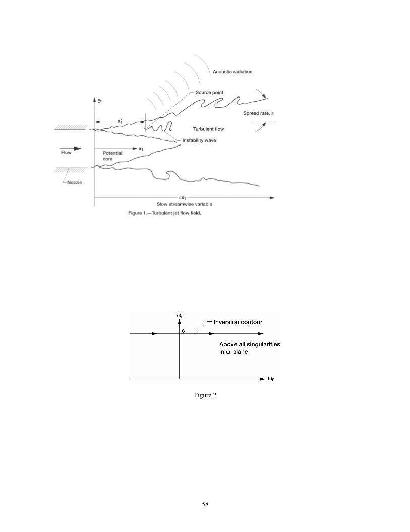
58
Figure 2
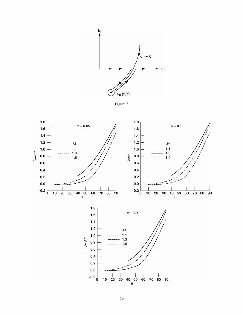
59
Figure 3
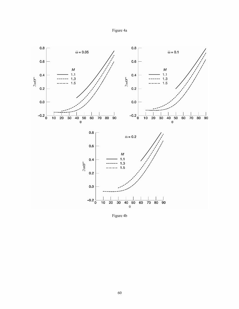
60
Figure 4a
Figure 4b
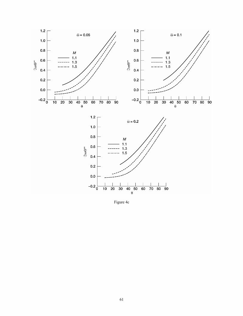
61
Figure 4c
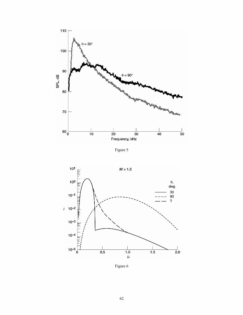
62
Figure 5
Figure 6
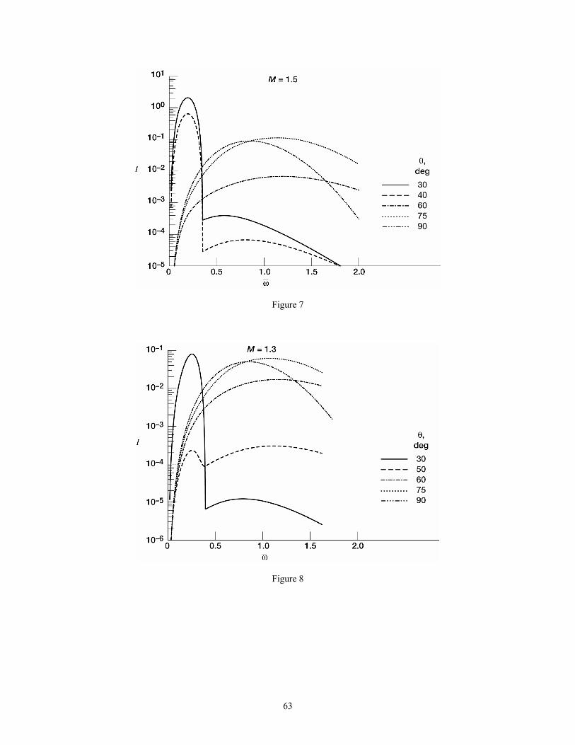
63
Figure 7
Figure 8
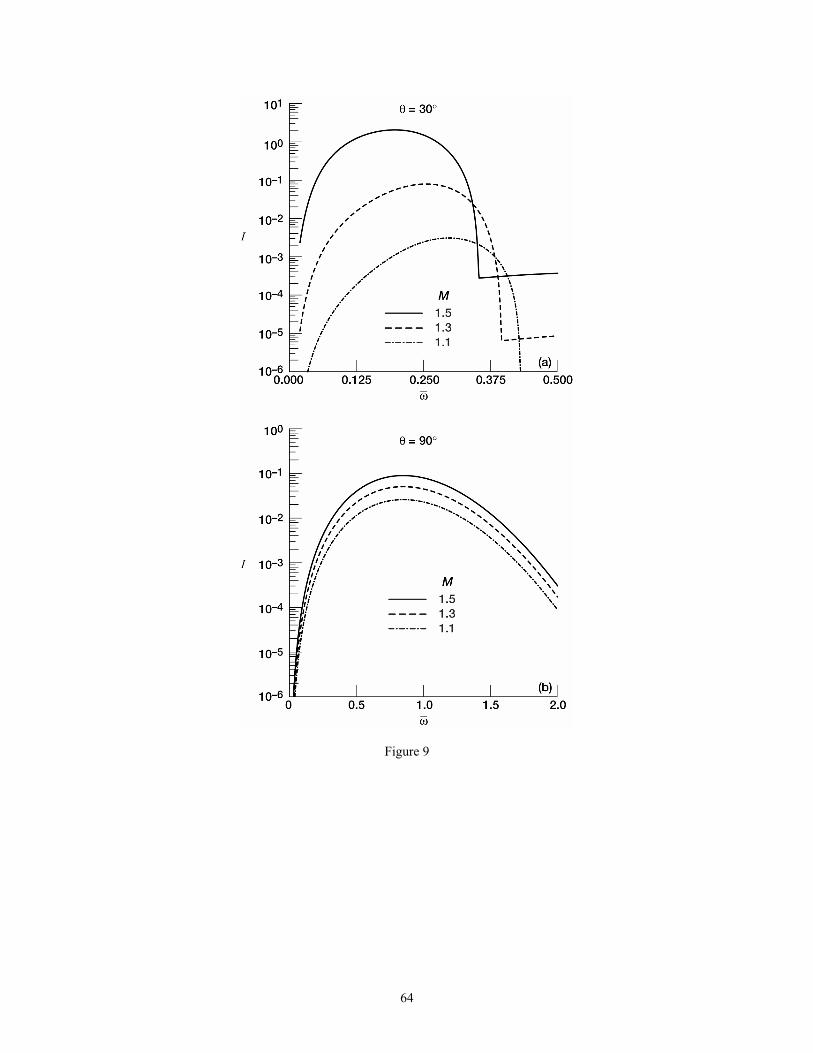
64
Figure 9
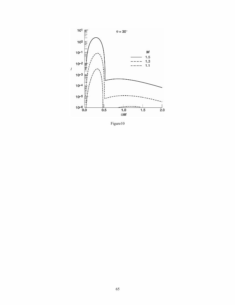
65
Figure10
Related Documents