The Role of Illiquidity Risk Factor In Asset Pricing ...journalarticle.ukm.my/8075/1/834-1591-1-SM.pdf · Jurnal Pengurusan 26(2007) 67-97 The Role of Illiquidity Risk Factor In Asset

Jurnal Pengurusan 26(2007) 67-97

The Role of Illiquidity Risk Factor In Asset Pricing Models: Malaysian Evidence

Ruzita Abdul Rahim Abu Hassau Shaari Mohd_ Nor

ABSTRACT

'fhis paper examines the role of illiquidity risk factor in asset Prlczng through two variants of liquidity-based three-factor models, referred as SiLiq and DiLiq, which are developed in the context of Fama-French model. The sample comprises 230 to 480 firms which stocks are listed on Bursa Malaysia over the period of January 1987 to December 2004. To proxy for liquidity, this study tests six alternative measures based on trading volume variables, namely dollar volume (DVOL), share turnover (TURN), Illiquidity (ILLlQ), and the coefficient of variations of each of these variables (CV

DVOL"

cVrURN" and cV1UJoY. The preliminary results indicate that the illiquidity risk

factors (i.Mil) that are formed from TURN consistently outperform the other alternatives as they explain as high as 36 percent variations in stock returns. The results of multiple time series regressions lend strong support for the

hypothesis that illiquidity risk are priced, particularly when is LMH incorporated in DiLiq.

ABSTRAK

Kertas ini meguji peranan risiko ketakcairan dalam penetapan harga aset melalut dua varian model tiga-factor berasaskan kecairan, dirujuk sebagai SiLiq dan DiLiq, yang dibentuk dalam konteks model Fama-French. Sampel kajian merangkumi 230 hingga 480 syarikat yang sahamnya disenaraikan di Bursa Malaysia bagi tempoh Januari 1987 hingga Disember 2004. Untuk menentukan proksi bagi kecairan, kajian ini menguji enam ukuran alternati! berasaskan valum dagangan iaitu nitai valum dagangan (DVDL), pusingganti saham (TURN), ketakcairan (IUIQ), dan kaefisyen variasi bagi setiap satu ukuran tersebut ((CVDVOL" CVTURN" and cV,w,)' Hasil preliminari kajian

menunjukkanfaktor-faktor risiko ketakcairan (LMH! yang dibentuk daripada TURN secara konsisten mengatasi ukuran alternatif lain setelah didapati ia menjelaskan 36 peratus variasi dalam pUlangan saham. Hasil daripada regresi siri masa berganda memberikan sakangan kuat terhadap hipatesis

bahawa risiko ketakcairan diganjari, khususnya apabila LMH diambilkira dalam DiLiq.

68 Jurnal Pengurusan 26

INTRODUCTION

The empirical frustration over the capital asset pricing model (CAPM) of Sharpe (1964), Lintner (1965), and Black (1972) has always been identified as the main motivation for the development of multifactor models such as Intertemporal CAPM (ICAPM) (Merton 1973) and Arbitrage Pricing Theory (APT) (Ross 1976). Despite the theoretical appeal, these conventional multifactor models suffer the same problem of empirical testability as CAPM.

While the CAPM is rigid in claiming that market risk alone is sufficient to explain asset prices, the ICAPM and APT are silent regarding what and how many factors are priced (Fama 1998). The empirical failures of conventional models led to the development of another variant of asset pricing model termed empirical multifactor models (Hodrick & Zhang 2001). The simplicity in developing these models undoubtedly explains the attention, but its widespread acceptance owes as much to the success story of a three-factor model introduced by Fama and French (1993). The Fama-French model specifies that expected excess returns on stock i (E(R,!-RF) is,

(1)

where E(.) is the expected operator, RM - RF is the market risk premium, 5MB is the premium on risks related to size, HML is the premium on risks related to distress, and b., s., and d. are the coefficients or sensitivity of R. to the premiums on thd r~spectiv~ risk factors. Even though lacking i~ underlying theories, the model has been successful in explaining most major anomalies of the conventional models (Fama & French 1996a).

The evidence that Fama-French model is superior to the CAPM or the market model is indisputably convincing. However, as more studies are devoted to examine the effectiveness andlor application of Fama-French model, contradicting evidence also accumulates (cf. Bartboldy & Peare 2005; Daniel & Titman 1997; Hodrick & Zhang 2001; Jaganathan & Wang 1996). The mixed results, reinforced by Fama and French's (1996a) own conclusion that there is weakness in their model, imply the needs for continuing the search for other more effective empirical multifactor models. Of main interest to the present study are those that focus on the role of liquidity factor in extending the standard CAPM or Fama-French model (Bali & Cakici 2004; Chan & Faff 2005; Chollete 2004; La & Wang 2001; Liu 2004; Miralles & Miralles 2005). Particularly because Fama-French model is an implication of ICAPM (Fama & French 1993, 1996a), there is a great potential that liquidity is the omitted factor in the model (Hodrick & Zhang 2001) because it is a state variable in the ICAPM sense (Chollete 2004). This conjecture is also consistent with the role that liquidity plays as one of the determinant of returns on fixed income securities. In short, had it not for the

The Role of Illiquidity Risk Factor 69

difficulty to find the right measurement for liquidity (Keown et al. 1996), the factor must have been considered as one determinant of stock returns much sooner. For the present study, liquidity is of utmost relevant because the sample market, Bursa Malaysia, is an ideal setting to examine its role in asset pricing. As Rouwenhorst (1999), Bekaert et al. (2005) and Dey (2005) asserted, liquidity is one firm characteristic that is of particular concern to investors in emerging market.

To examine the role of liquidity in asset pricing models, this study uses data on a sample of 230 to 480 companies listed on Bursa Malaysia over the period of 18-year from January 1987 to December 2004to. For robustness, six alternative measures of liquidity based on trading volume variables are tested, namely dollar volume, share turnover, illiquidity, and the coefficient variations of each of the variables. Used alone, the liquidity measure proves to capture significant fractions of variations in stock returns. Of more interest to this study is the role of liquidity in multifactor model. This is examined by developing two variants of Fama-French model which incorporate the illiquidity risk factor. The results obtained through multiple time series regressions in general confirm the prediction that illiquidity risks are priced for stocks traded in Bursa Malaysia. The remainder of the article is organized as follows. Section 2 presents the background studies. Section 3 describes the data and methodology. Section 4 reports the empirical results while and section 5 concludes.

BACKGROUND STUDIES

Liquidity is generally defined as the ability to trade quickly at low cost with little price impact. The theoretical role of liquidity in asset pricing has long been documented in your finance textbooks (cf., Brigham, Gapenski & Ehrhardt 1999; Keown, Scott, & Martin 1996) whereby liquidity is normally described as one other type of risk premium that helps to determine interest rate on fixed income assets. Therefore, it is just natural that liquidity quickly captures financial economies' attention after Fama and French (1996a) concluded that there is still loophole in their model. Specifically, Chollete (2004; I) asserted that "". liquidity is a natural choice as an asset pricing factor since it is a state variable in the ICAPM sense". This statement is consistent with Hodrick and Zhang's (2001) suggestion regarding the possibility of liquidity factor to be the omitted variable in the existing asset pricing models.

Despite the theoretical support, only recently has the role of liquidity in asset pricing models been tested empirically. One possible explanation to the delay is the difficulty to find the measurement for liquidity (Keown et al. 1996). Liquidity is an elusive concept which involves multiple dimensions-

70 Jurnal PenJ?urusan 26

trading quantity, trading speed, trading costs and price impact. So far, none of the suggested proxies has been successful to capture all of these dimensions. Despite being recognized as the more direct, first class measure of liquidity (Lesmond 2005), the bid-ask spread of Amihud and Mendelson (1986) only concentrates on the trading costs. The difficulty to find sufficient data on bid-ask and other direct measures of liquidity further delays the incorporation of liquidity in asset pricing studies.

The need for more accessible alternative measures lead a number of researchers to resort to trading volume variables, the second class liquidity measure (Lesmond 2005). For the purpose of this study, the discussion concentrates on three basic variables, namely share turnover (TURN), dollar volume (DVOL), and illiquidity (ILLIQ). In proposing illiquidity, Amihud (2002) argued that trading activity is a good proxy of liquidity because liquidity is the impact of order flows on price resulting from adverse selection and inventory costs. The viability of volume-based variables as measure of liquidity has also been empirically supported by findings of several studies (cf. Bekaert, Harvey, & Lundblad 2005; Lesmond 2005; Liu 2004) which found that volume-based liquidity measures are highly correlated with the bid-ask spread. In addition, the notion that volume-based liquidity determine asset pricing almost naturally fits into the mindset given the long history of relationship that trading volume has with stock returns (Karpoff 1987). To the Wall Street professionals volume is the fuel that drives stock prices (Hameed & Ting 2000; Moosa & AI-Loughani 1995; Stickel & Verrechia 1994).

An important advantage of volume-based liquidity is in terms of available data. However, like bid-ask spread these volume-trading measures also fail to capture all of the dimensions of liquidity. Turnover (Datar, Naik & Radcliffe 1998) captures only the trading quantity dimension whereas the illiquidity (Amihud 2002; Pastor & Stambaugh 2003) focus only on the price impact. The search for alternative measure of liquidity is beyond the scope of this study which immediate interest is on the role of volume-based liquidity in explaining variations in portfolio returns.

The relationships between various volume-based measures of liquidity and stock returns are sufficiently represented by the results of 20 related studies summarized in Table 1. In short, if volume-based variables are sufficient representation of liquidity, then the results in Table I lend a strong support for the theoretical prediction regarding the role of liquidity as an important driver of expected stock returns. Specifically, three studies that employed DVOL (Brennan, Chordia, & Subrahmanyam 1998; Chordia, Subrahmanyam, & Anshuman 200 I; Spiegel & Wang 2005) indicated that its relationship with stock returns is significant and most of the times negative. Of nine studies that used TURN all including Rouwenhorst (1999) supported the role of liquidity in explaining stock returns. Given the

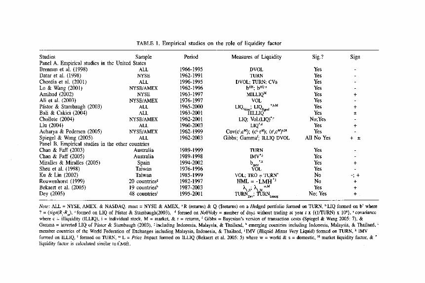
TABLE 1. Empirical studies on the role of liquidity factor

Studies Sample Period Measures of Liquidity Panel A. Empirical studies in the United States Brennan et a!. (1998) ALL 1966-1995 DVOL Datar et al. (1998) NYSE 1962-1991 TURN Chordia et a!. (2001) ALL 1996-1995 DVOL; TURN; CVs Lo & Wang (2001) NYSE/AMEX 1962-1996 bHR; bHQ a

Amihud (2002) NYSE 1963-1997 MILLIQM Ali et a!. (2003) NYSE/AMEX 1976-1997 VOL Pastor & Stambaugh (2003) ALL 1965-2000 LIQval ... ; LIQ~"al ",b,M

Bali & Cakici (2004) ALL 1963-2001 HILLIQ Chollete (2004) NYSEIAMEX 1962-2001 LIQ; Vo1.(LIQ)'·o Liu (2004) ALL 1960-2003 LIQ*,d Acharya & Pedersen (2005) NYSE/AMEX 1962-1999 Cov(d,cM); (d'rAl); (ri,cM)e,M Spiegel & Wang (2005) ALL 1962-2003 Gibbs; Gammaf ; ILLlQ DVOL Panel B. Empirical studies in the other countries Chan & Faff (2003) Australia 1989-1999 TURN Chan & Faff (2005) Australia 1989-1998 IMV'j Miralles & Miralles (2005) Spain 1994-2002 blMV '.' Sheu et a!. (1998) Taiwan 1976-1996 VOL Ku & Lin (2002) Taiwan 1985-1999 VOL; lRO = TURN' Rouwenhorst (1999) 20 countriesg 1982-1997 HML= -LMH" Bekaert et a!. (2005) 19 countriesh 1987-2003 ).. . \. m.M

LS' W Dey (2005) 48 countriesi 1995-2001 TURN~v; TURNEmerg

Sig.?

Yes Yes Yes Yes Yes Yes Yes Yes

No;Yes Yes Yes

All No Yes

Yes Yes Yes Yes No No Yes

No; Yes

Sign

+

+ ±

+

+ ±

+

-; + + + +

Note: ALL = NYSE, AMEX, & NASDAQ, most = NYSE & AMEX,"R (returns) & Q ($retums) on a Hedged portfolio formed on TURN, bLIQ fonned on b! where ? = (sign(R,-R

M), 'fanned on LIQ of Pastor & Stambaugh(2003), d formed on NoOVoly = number of days without trading at year t x {(lfTURN) x 106}, <covariance

where c = illiquidity (ILLIQ), i = individual stock, M = market, & r = returns, f Gibbs = Bayesian's version of transaction costs (Spiegel & Wang 2005: 7), & Gamma = inverted LIQ of Pastor & Stambaugh (2003), g including Indonesia, Malaysia, & Thailand, h emerging countries including Indonesia, Malaysia, & Thailand, i

member countries of the World Federation of Exchanges including Malaysia, Indonesia, & Thailand, j IMV (ntiquid Minus Very Liquid) formed on TURN, k IMV formed on ILLIQ, I formed· on TURN, m L = Price Impact formed on ILLIQ (Bekaert et al. 2005: 5) where w = world & s = domestic, M market liquidity factor, & • liquidity factor is calculated similar to LMH.


insignificant premium on liquidity risk factor, Rouwenhorst (1999) concluded that the role of liquidity factor is trivial. However, such inference seems to be preliminary because other studies (Drew & Veeraraghavan 2003; Chan & Faff 2005; Miralles & Miralles 2005) had shown that premium does not necessarily deduce to insignificant role the respective factor plays in asset pricing model. In the mean time, except for Spiegel and Wang (2005), five other studies that used ILLIQ also suggested that liquidity has an important driver of stock returns.

In the meantime, there are eight studies marked with asterisks in Table 1 that examined liquidity in the context of Fama-Fama model. Using various basic volume-based variables, these studies presented liquidity factor in relative form to focus on the premium expected for assuming greater illiquidity risks. Five of them (Bali & Cakici 2004; Chan & Faff 2005; Chollete 2004, Liu 2004, Miralles & Miralles 2005) are particularly relevant to the present study because they also examined the role of illiquidity risk in time series regression proposed by Black, Jensen, and Scholes (1972), the same manner in which the Fama-French model was developed. Except for Chollete (2004), these studies produced results that are lenient toward supporting that illiquidity risks are priced. Overall, all of these studies are unanimously in favor of the asset pricing models that incorporate a liquidity factor over those that do not.

DATA AND METHODOLOGY

The present study uses data for 230 to 480 companies that are listed in the Main Board of Bursa Malaysia for the period of l8-year from January 1987 to December 2004. Two sets of data are used; (i) monthly data on stock closing prices, rate of returns on three-month Treasury Bills (T-Bills), and price index of Exchange Main Board All Shares (EMAS), and (ii) year-end data on number of shares outstanding (NOSH), trading volume (VOL), market value of equity (ME), and book-to-market ratio (BIM). The data is sourced from Thompson's DataStream and Investors' Digest. The selection criteria for the sample firms are mainly based on the availability of data.

THE DEPENDENT VARIABLES

The dependent variables to be explained in this study are the excess realized returns on the test portfolios. These are monthly value weighted-average rate of returns on test portfolios net of the risk-free rate of returns (R(R

F). To

construct the test portfolio, at the end of December of each year 1-1 the sample stocks will be sorted into: (i) three ME categories i.e., 30 percent smallest (S), 40 percent medium (M), and 30 percent biggest (B); (ii) three BI M categories i.e., 30 percent highest (H), 40 percent medium (M), and 30

The Role oj Illiquidity Risk Factor 73

percent lowest (L); and (iii) three TURN categories i.e., 30 percent lowest (L),

40 percent medium (M'), and 30 percent highest (Ii). The intersections of the three ME and BIM categories generate the first group of 9 MElBM test portfolios, the intersections of the three ME and TURN categories generate the second group of 9 MEIfURN test portfolios and three B/M and TURN categories generate the last group of 9 BMIfURN test portfolios. The same procedure of reconstructing the portfolios and calculating their value-weighted returns will be repeated at the end of each of the 18-year study period.

THE BASIC RISK FACTORS

The basic explanatory factors in this study are the market risk premium (RM

- Rp) and the premiums on risks related to size (SMB) and distress (HML)

proposed by Fama and French (1993). This study chooses EMAS over the Kuala Lumpur Composite Index (KLCI) to proxy for market portfolio for the reason that the former is more representative of the sample popUlation, i.e., companies listed on Main Board. Unlike KLCI which is based on 100 component stocks, EMAS is composed of all stocks listed in the Main Board. This explanation conforms to the construction of market portfolio which includes all stocks listed on NYSE, NASDAQ and AMEX in previous studies (cf. Fama & French 1992, 1993, 1996a; Davis, Fama, & French. 2000; Chollete 2004) despite the existing broad-based indexes that are readily available. The proxy for the risk-free rate of return (Rp) is the monthlyadjusted-rate of return on Malaysian 3-month Treasury Bills.

To construct 5MB and HML, zero-investment portfolios that mimic risk related to size (as proxied by ME) and distress (as proxied by B/M) are constructed using the same procedure to form the test portfolios (except for ME categories that are only divided into Sand B categories). Specifically, in the manner similar to Fama and French (1993), 5MB and HML are expressed as,

(2)

(3)

where R is the value-weighted rate of returns on the ME/BM test portfolios. The procedures in Equations (3) and (4) ensure that the premium on size (distress) risk is relatively free from the influence of distress risk because the Small and Big (High and Low) portfolios have about the same weightedaverage BIM (ME).


THE ILLIQUIDITY RISK FAcroR

For robustness, this study identifies several liquidity measures based on volume data that are frequently used in previous studies (Acharya & Pedersen 2005; Amihud 2002; Bali & Cakici 2004; Brennan et aI. 1998; Chan & Faff 2003,2005; Chordia & Swaminathan 2000; Chordia et al.2001; Datar et al. 1998; Ku & Lin 2002; Miralles & Miralles 2005; Rouwenhorst 1999). The selected variables are as follows;

DVOL j,t = Pj,/xVOL j,t.

VOLj,1 TURN j.' - NOSH. '

;.<

a UQ CV = __ J_.' uQj,1 II '

rUQj,1

(4)

(5)

(6)

(7)

where VOL. is volume of shares j, NOSH. is number of shares j outstanding, J J

P is the price per share j, DVOL. is dollar volume of share j, TURN. is the J J J

turnover of share j, ILLlQj

is illiquidity of share j, IR i,1 is the absolute return

on share j, cv is the coefficient of variation of the liquidity measure, LlQ = DVOL, TURN, or ILLIQ, S is the standard deviation for the time series LlQ, and m is the average of the time series uQ at the end of year t. Next, in a similar manner that 5MB and HML are formed, the premium on risks related to

liquidity, denoted as LMH is calculated as;

£Mit _(RS!L +RB!L )_(RSIH +RBIH ) MEILlQ - 2 2' and (8)

(9)

where the definitions are as in Equations (3) to (7). The construction of

LMH is consistent with the liquidity theory which posits that stocks with low levels of trading volume are less liquid and therefore command higher

returns. In other words, the premium on liquidity risk (LMH) essentially

The Role oj Illiquidity Risk Factor 75

reflects the premium that investors would require for holding less liquid stocks as they anticipate higher trading costs when reselling the stocks in the future (Datar et al. 1998; Dey 2005). Equation (8) produces 6 alternative LMH measures, i.e. from the intersections between ME and each of the alternative liquidity (LIQ) measures in Equations (4) to (7). Similarly, Equation (9) produces another set of 6 alternative LMH measures from the intersections between BIM and each of the 6 alternative LIQ measures.

THE DEVELOPMENT OF THE LIQUIDITY-BASED MODELS

In the spirit of earlier studies (Bali & Cakici 2004; Chollete 2004; Chan & Faff 2005; Miralles & Miralles 2005), the present study assigns to liquidity a role of stock's common risk factor in the context of Farna-French model. The Fama-French model was developed based on time series regression proposed by Black et al. (1972). This approach proposes that the average risk premium on a common factor in stock returns is the average value of the explanatory factor. The premium per unit of market risk (RM-R

F) is

defined as the difference between the return on market portfolio (RJ and the average returns on risk-free securities (R

F). Farna and French (1993) adopted

this principle to define the additional risk factors (SMB and HML) in their model. Unlike previous studies (Bali & Cakici 2004; Chollete 2004; Chan & Faff 2005; Miralles & Miralles 2005) which incorporate liquidity as an additional risk factor in the standard Farna-French model, the present study deviates slightly in the sense that it incorporates liquidity as an alternative factor to Farna-French factors to develop two variants of the three-factor model. In that respect, not only this study examines the role of liquidity in asset pricing model, it simultaneously tests Fama and French's (1996a) proposition that three-factor models suffice to explain stock returns.

We next proceed with the development of two variants of the three-

factor model that incorporate the role of liquidity as proxied by LMH. To show how these models differ from the Farna-French model, we first rewrite the Fama-French model time-series regression equation,

where R; is the realized returns on portfolio i, i = 1, . ,.,27, Q; is the intercept, h" s" and d, are the estimated factor loadings for portfolio i, RM is the realized rate of returns on the market portfolio as proxied by the EMAS

index, RF is the rate of return on the risk-free security as proxied by the TBill, 5MB

FF and HMLFF are respectively the premium on size and distress

factors formed from the intersections of MEIBM portfolios, and e, is the disturbance term at the end of month t.


In line with the development of other extended Fama-French models (Bali & Cakici 2004; Chan & Faff 2005; Miralles & Miralles 2005), the market risk premium (RM-R

F) remains the main risk factor in the liquidity

based models. The first variant of the model combines market risk premium

(RM-RF

) with "Size" (SMB) and replace HML with uQuidity (LMH) to form "SiLiq" model,

The second variant of the liquidity-based model drops 5MB to form "DiLiq" as a combination of market risk premium (RM-R

F), "DIstress" (HML) and

"LIQuidity" (LMH),

where definitions of a;, hp s;, d;, R;, RM, RF' and e; remain as in Equation (l0),

I; is the slope on LMH, 5MB UQ.' is the size risk factor formed from the intersection of ME/TURN portfolios, HML

UQ" is the distress risk factor fanned

from the intersection of BMiTURN portfolios, and LMH. in Equations (4) and J'

(5) are the proxy for illiquidity risk factors formed from the intersection of MEfTIJRN and BMrruRN portfolios at the end of month t, respectively.

THE STATISTICAL TESTS

Following Fama and French (1993, 1996a), multiple time series regressions of Black et aI. (1972) are used to estimate monthly excess returns on test portfolios using the alternative three-factor models as specified in Equations (10) to (II). Fama and French (1993) explained that the slopes and R' in time series regressions are direct tests on the role of a particular risk factor in an asset pricing model. The T-statistics on the slope (?) is calculated as,

Pi

-f3jO) T s- (13)

Pi

where Pi is the loading (slope) of explanatory factor j, j = RM-RF

, 5MB, HML,

s~ _ s .J n -1 is the standard error of f3 jo Sy/,is the estimated

x

standard deviation in time series y and y given x, and n is number of time series data. In the context of an asset pricing model, a risk factor is priced if the null hypothesis of' Ho: f3 = O' is rejected, i.e., when ITI " tN_2. l~'


The role of a particular factor in an estimated model can be tested with the T-statistics, but of more importance to an asset pricing model is the contribution of the factor in generating the most efficient model to explain the returns of test assets. Previous studies (c.f. Davis et aI. 2000; Fama & French 1996a) employed R2, a quantitative measure of goodness-of-fit, to evaluate the efficiency of a k-factor model in explaining returns of stocks or portfolios of stocks, which is defined as,

N

L(Y' _f)2 R' = RSS = -'~~' __ _

TSS N

L(y,-f)' (14)

,-I

where RSS is the total variations that can be explained with the regression model and TSS is the total actual variations in Y. Because R' tends to increases with the number of explanatory variables, it is adjusted to,

Ad'R' R-2 1 ( 2)",-1 ~- c= . = - I-R. -I I r ni-k, (15)

where R,' is the R2 from model i, i = Fama-French, SiLiq, or DiLiq models,

n; is the number of observations in the time series data in model i, and ki

is the number of parameters in model i.

In addition to an R2 value of 1.0, an efficient asset pricing model requires zero regression intercept (Daniel & Titman 1997; Davis et aJ. 2000; Drew & Veeraraghavan 2002, 2003; Faroa & French 1993, 1994, 1995, 1996a, 1998; Leledakis & Davidson 2001). The null hypothesis Ho: a, = 0 is tested using the T-statistics on the intercept (a),

" (0)

T = U i -at apabila a~O) = 0.0, Sai

(16)

where a, is the intercept for regression of Equation i,i = Equation (10), (11),

I X' , or (12). Sa; =Syll ~+ (n-l)S; is the standard error for ai, Sy/x is the

estimated standard deviation in time series data y and y given x, X' is the average value of x squared, n is the number of time series data, and S} is the estimated variance for time series data x. The null hypothesis Ho: a

i = 0.0


is rejected if ITI " t".2. J.a12' In short, if the results of the regression of the kfactor model generates R2 = 1.0 and a = 0.0, the model is said to be an efficient model because it explains all variations in expected returns.

EMPIRICAL RESULTS

PRELIMINARY RESULTS

Table 2 presents the descriptive statistics of the time series data of each of 27 test portfolios and 7 explanatory factors. In Panel A, notwithstanding the fact that the highest monthly excess return (and standard deviation) is reported by portfolio SL, the average monthly excess returns in general tend to decline monotonically from the riskiest (SH) to the least risky (BL) portfolios. Also, consistent with Drew and Veeraraghavan (2002), the monthly excess returns for the S's portfolios are significant, indicating existence of size premium in Malaysian stock market. The monthly excess returns on MEl

TURN portfolios reported in Panel B also exhibit similar monotonically declining trend, only smaller and somewhat less consistently. Specifically, in each size category returns on portfolio L' (low turnover) are consistently higher than returns on portfolio H' (high turnover). The same patterns are observed on monthly excess returns in Panel C. Such contradiction to riskreturn trade-off theory fortunately is nothing new to studies in emerging markets (Pastor & Starobaugh 2003; Rouwenhorst 1999). The monthly excess returns in Panel C are smaller than those in other Panels and the patterns are also less definite.

Table 3 reports the descriptive statistics of and correlation coefficients between the explanatory factors. Panel A shows that only premiums on risks related to size (SMB's) are significantly greater than zero. The premiums on risks related to distress (HML'S) are positive but insignificant. Interestingly, the premiums on market risks and illiquidity risks are negative. Although insignificant, these results contradict the risk-return trade-off which posits that riskier assets must be compensated with higher returns (premiums). However, these findings could serve as support for our earlier proposition that existence of premiums do not necessarily deduce to the insignificant role the factors in asset pricing model (Drew & Veeraraghavan 2003; Chan & Faff 2005; Miralles & Miralles 2005; Rouwenhorst 1999). Panels B and C report the correlations aroong explanatory factors of the alternative three- factor models.

The correlations in Panel B highlight the advantage of Fama-French model for having formed by relatively independent explanatory factors (Fama & French 1966a). The correlations among the explanatory factors of Faroa-French model, which are within the range of 0.244 to 0.356, are lower than those of SiLiq (-0.575 to 0.382) and DiLiq (-0.606 to 0.489).

TABLE 2. Descriptive statistics of time series data, 1986:01 - 2004:12

Panel A. Monthly Excess Returns on Nine ME/BM Test Portfolios Statistics SH SM SL MH MM ML BH BM BL Mean 0.026 0.023 0.030 0.016 0.010 0.009 0.011 0.009 0.004 T-stats 2.434* 2.368* 2.685** 1.827* 1.238 1.110 1.156 1.311 0.621 Std. Dev 0.159 0.145 0.162 0.131 0.117 0.122 0.145 0.099 0.084 Skewness 1.734 1.756 1.639 1.356 1.466 1.381 2.592 1.091 0.143 Kurtosis 9.050 9.646 7.986 7.880 8.443 8.227 18.384 9.463 4.662 J-B Stats 437.7** 508.6** 320.5** 280.6** 344.0** 314.6** 2371.9** 418.8** 25.58** ADF Stats -4.04** -4.39** -4.44** -3.84** -3.92** -4.33** -4.18** -3.89** -3.71** Panel B: Monthly Excess Returns on Nine MEITURN Test Portfolios Statistics sL SM SH ML MM MH BL BM BH Mean 0.019 0.029 0.026 0.007 0.013 0.016 0.007 0.004 0.009 T-stats 2.209* 2.761** 2.492* 1.057 1.530 1.623 1.151 0.724 1.217 Std. Dev 0.126 0.154 0.155 0.101 0.123 0.143 0.084 0.089 0.109 Skewness 1.212 1.644 1.270 1.444 1.198 1.396 1.024 0.269 0.155 Kurtosis 6.887 8.471 5.952 9.076 6.875 7.881 7.643 6.045 4.483 J-B Stats 188.9** 366.6** 136.5** 407.3** 186.8** 284.6** 231.7** 86.05** 20.67** ADF Stats -3.94** -4.67** -4.41 ** -4.08** -3.87** -4.09** -4.05** -3.70** -3.83** Panel C. Monthly E~cess Returns on Nine BMlTURN Test P,:rtfolios

MH LL L11 Statistics HL HM HH ML MM LM Mean 0.011 0.015 0.D18 0.007 0.011 0.014 0.006 0.003 0.009 T-stats 1.455 1.573 1.687 1.056 1.500 1.612 0.948 0.444 1.262 Std. Dev 0.109 0.137 0.158 0.094 0.106 0.126 0.086 0.085 0.110 Skewness 1.356 2.190 1.867 1.470 1.122 1.080 1.716 0.086 0.198 Kurtosis 8.011 15.303 11.621 10.151 8.978 7.170 13.123 4.894 3.980 J-B Stats 292.3** 1534.9** 794.4** 538.1 ** 366.9** 198.53** 1028.2** 32.54** 10.05** ADF Stats -3.84** -3.95** -4.25** -3.75** -3.93** -4.02** -4.77** -3.56** -3.67**

Note: (1) N = 216 monthly observations. Lag length for the Augmented Dickey-Fuller (ADF) test is 12, (2) Asterisks ** and * denote significance at 1 percent and 5 percent levels.

TABLE 3. Descriptive statistics of and correlation coefficients between explanator factors

Panel A. Monthly Excess Returns on Seven Explanatory Factors Statistics R,.-R, 5MBA' 5MBMT HML" HMLBT LMHMT Mean -0.003 0.012 0.012 0.004 0.009 -0.005 t-stats -0.480 2.896** 2.681 ** 0.993 1.637 -1.424 Std. Dev 0.088 0.061 0.068 0.060 0.078 0.051 Skewness 0.148 1.795 1.655 1.803 3.166 -0.303 Kurtosis 5.507 9.892 10.440 17.755 27.801 5.645 J-B Stats 57.33** 543.48** 596.72** 2076.46** 5896.53** 66.28** ADF Stats -3.744** -4.295** -4.051 ** -4.026** -3.839** -4.112** Panel B. Correlation Coefficients between Explanatory Factors in Fama-French Model Factors RM-R, 5MB" HMLA' RM-Rp 1.000

5MB" 0.345**· 1.000

HML" 0.356** 0.244** 1.000 Panel C. Correlation Coefficients between Explanatory Factors in Liquidity-Based Multifactor Model Factors R,.-R, 5MBMT LMHMT Factors R,.-R, HMLBT RM-Rp 1.000 RM-Rp 1.000 5MBMT 0.382** 1.000 HML'T 0.489*' 1.000 LMHMT -0.575** -0.425** 1.000 LMHBT -0.606** -0.496**

Note: (I) N = 216 monthly observations. Lag length for the Augmented Dickey-Fuller (ADF) test is 12. (2) Subscripts FF = Fama-French, MT = intersections between ME and TURN and BT = intersections between BM and TURN. (3) Asterisks "'* and'" denote significance at 1 percent and 5 percent levels.

LMHBT -0.006 -1.553 0.057 -0.385 5.393

56.86** -4.361 **

LMHBT

1.000


The remaining details in Tables 2 and 3 are pertaining to the appropriateness of the time series analysis used. Specifically, statistics of first moments indicate that all return series except the LMH's are positively skewed, with fat tails. The resulting Jarque-Bera (J-B) statistics suggest that the null hypothesis of normal distribution is consistently rejected at I percent significant level, a finding which is normal when involves stock return series (Bali & Cakici 2004). Of more importance to time series analysis is the stationarity of the series, which are confirmed by the Augmented Dickey-Fuller (ADF) statistics. That is, the null hypothesis of unit root is consistently rejected at I percent level of significance.

For the purpose of developing the liquidity-based models, this study selects only one from each of two groups of alternative measures following the approach suggested in Madalla (2001) and Bartholdy and Peare (2005).

The approach posits that where exist several alternative LMH measures for a variable, select one that generates the highest R2 from a univariate regression. Table 4 only reports the selective details to conserve space. The

results show that LMH that are formed from TURN (and ME or BIM

intersections) consistently generate the highest adjusted R'. Accordingly, these measures are selected as proxy for illiquidity risk factor for the development of the liquidity-based three-factor models in this study. In the

remainder of this article, LMH always refers to these measures only. It is also important to note that the results in Table 4 are crucial initial evidence supporting the role of liquidity factor in asset pricing models given that used

alone, LMiI explain 30 to 36 percent of variations in stock returns.

TESTS ON CAPITAL ASSET PRICING MODEL

It is a standard practice in studies on asset pricing to begin with tests on the CAPM. The results displayed in Table 5 indicate that consistent with previous studies (e.g., Bali & Cakici 2004; Fama & French 1993, 1996a), the market risk premium captures most of the variations in expected returns. Consistent with Clare, Priestley, and Thomas (1998) and Farna and French's (l996b) assertion that beta is still alive, the slopes on market risk are always positive and greater than 17 standard errors from zero (average?t?29.1). It also provides strong justification for the role market risk has as the main risk factor in multifactor models. However, the resulting R2 which average 76.7% suggests that market risk leaves plenty of variations in stock returns to be explained by other factors. Only in one portfolio under each category of test portfolios do the adjusted R' of CAPM is greater than 90%. Also, the highly significant role of market risk in explaining stock returns supports earlier conjecture that existence of premium associated to a risk factor is no

TABLE 4. Summary of results of time series univariate regressions, 1987:01 - 2004:12

Panel A: LMH from MEJLIQ; intersections Panel B: LMH from BM/LIQ; intersections Average (.) I t(l) Adj-R' Average (.) L t(l) Adj-R'

LMHMElDVOL -0.937 -5.144 (9/9) 0.1082 LMHBMfDVOL -0.463 -3.032 (5/9) 0.0548

LMHMElC'V(DVOL) -1.079 -6.745 (9/9) 0.1763 LMHBM/CV(DVOL) -0.630 -4.126 (7/9) 0.0848

LMHME/CV(TURN) -0.995 -5.316 (9/9) 0.1199 LMHBM/CV(TURN) -0.687 -3.958 (7/9) 0.0793

LMHMEllLLlQ 0.525 2.138 (8/9) 0.0293 LMHBMIlLLlQ 0.337 1.614 (719) 0.0350

LMHMElCV(ILLlQ) 0.596 3.875 (9/9) 0.0628 LMHBM/CV(ILLlQ) 0.519 3.013 (8/9) 0.0391

LMHMffiURN LMHBMrrURN

SH -1.808 -10.281** 0.3275 SH -1.712 -11.475** 0.3780 SM -1.702 -10.806** 0.3500 SM -1.562 -11.499** 0.3790 SL -1.717 -9.360** 0.2872 SL -1.771 -11.871*' 0.3942 MH -1.514 -10.555*' 0.3393 MH -1.540 -13.375'* 0.4528 MM -1.341 -10.468*' 0.3355 MM -1.364 -13.230'* 0.4473 ML -1.389 -10.389" 0.3322 ML -1.280 -11.108*' 0.3628 BH -1.436 -8.505** 0.2491 BH -1.488 -10.702** 0.3456 BM -0.964 -8.338** 0.2417 BM -0.911 -9.152** 0.2780 BL -0.764 -7.596** 0.2087 BL -0.673 -7.576** 0.2078 Average (.) -1.404 -9.589 (9/9) 0.2968 Average (.) -1.367 -11.11 (9/9) 0.3606

Note: (1) Asterisks ** and * denote significance at 1 percent and 5 percent levels. (2) Subscripts i in column heading refer to the alternative liquidity (LIQ) measures in Equations (4) to (7), i.e., DVOL, TURN, ILLIQ, or their coefficient of variations (CV DVOL' CV TURN' and CV ILLIQ)'

(3) Figure in parentheses indicate the number of portfolios with significant t(l).


indication of its role in asset pricing model. Furthermore, the magnitude of the regression intercepts (a), which are almost always significantly greater than zero, indicates that there are ontitted factors in the CAPM and accordingly a valid justification for multifactor models,

THE ROLE OF LIQUIDITY FACTOR IN MULTIFACTOR MODELS

Tables 6 to 8 present the results of regressing the alternative three-factor models-Fama-French model, SiLiq and DiLiq-to explain the excess returns on the three categories of ME/BM, MEITURN, and BMrrURN test portfolios. To set the stage, Table 6 shows that regardless of which multifactor models, the slopes on market risk premium (RM,R

F) are always positive and

highly significant (average 1 t 1 32.6) as they are when used alone in CAPM

(Table 5). Such finding implies that adding two risk factors in the model does not reduce the role of market risk and accordingly justifies market risk as the main concern in asset pricing. The results in Panel A of Table 6 show that HML and particularly 5MB have significant role in explaining stock returns. In absolute terms, the slopes on 5MB are always 2.8 standard errors from zero (average 1 t 110.7) whereas the slopes on HML are 3.6 standard errors from zero except for portfolio ML where the slope is only 0.8 (average?t?8.0). The role of 5MB is even stronger in SiLiq (Panel B). Its slopes score an average of 11.1 standard errors from zero in absolute tenn. In contrast, HML does not show a particular change in its role when incorporated in DiLiq (average 1 t I 7.5).

The main focus of this study is the role of illiquidity risk factor (LMH) Compared to the role of both 5MB and HML, (LMH) does not seem to capture

much variations in stock returns. This is particularly obvious for [MH in

SiLiq. Specifically, the slopes on LMH are only significantly different from zero in 1 portfolio. More encouraging results are observed in Panel C where

LMH is incorporated in DiLiq. Although smaller compared to 5MB and HML, the slopes on are significantly greater than zero in 6 of 9 portfolios with an average 1 t 1 of 2.8. Consistent with the different performance of the explanatory factors, the resulting average adjusted R2 of Fama-French model is 89.4%, slightly higher than that of SiLiq (86.2%) which in tum is slightly higher than that of DiLiq (84.7%). On a different ground that Fama and French (1993) initially used to evaluate the efficiency of their model, FamaFrench model generates adjusted R2 greater than 90% in 4 portfolios whereas SiLiq and DiLiq report 5 portfolios with adjusted R' greater than 90%. Comparisons at the individual portfolio level suggest that FamaFrench model has highest adjusted R2 in 5 portfolios while Siliq and DiLiq each has I and 3 highest adjusted R', respectively.

TABLE 5. Regression Results of the One-Factor Model (CAPM), 1987:01 - 2004:12

a B t(a) t(b) Adj-R' S.B. D-W Stat, Panel A: ME/BM Test Portfolios SH 0.0475 1.4727 7.1542** 21.8888** 0.6898 0.0898 1.5552 SM 0.0381 1.3054 5.9053** 19.9847** 0.6495 0.0872 1.7736 SL 0.0461 1.3551 5.8739** 17.0436** 0.5738 0.1062 1.9344 MH 0.0313 1.3144 7.2843** 30.1816** 0.8089 0.0582 1.9287 MM 0.0204 1.1978 5.8317** 33.8631 ** 0.8420 0.0472 1.9037 ML 0.0207 1.2246 5.2565** 30.6488** 0.8136 0.0534 1.9948 BH 0.0295 1.3947 5.4261 ** 25.3318** 0.7487 0.0735 1.8442 BM 0.0139 1.0561 6.1493** 46.2509** 0.9086 0.0305 1.7485 BL 0.0022 0.8899 0.9279 37.0366** 0.8644 0.0321 1.9067 Panel B: ME/TURN Test Portfolios sL 0.0286 1.1759 5.5591 ** 22.5445** 0.8896 0.0370 1.9089 SM 0.0476 1.4132 7.4127** 21.6982** 0.9329 0.0237 1.8296 SH 0.0457 1.4286 6.9949** 21.5552** 0.7501 0.0435 1.9786 ML 0.0113 1.0315 3.6491 ** 32.7570** 0.8202 0.0611 1.8318 MM 0.0260 1.2695 7.4697** 35.9221 ** 0.8571 0.0472 1.7440 MH 0.0354 1.4344 7.8304** 31.3323** 0.8329 0.0420 2.1064 BL 0.0028 0.8277 0.8804 25.4266** 0.6832 0.0885 1.7119 BM 0.0061 0.9686 3.4618** 54.6856** 0.6860 0.0870 1.6772 BH 0.0179 1.1542 6.5293** 41.6411** 0.7023 0.0696 1.8831

(Continued next page)

TABLE 5. (Continue)

Panel C: BMfTURN Test Portfolios HL 0.0177 1.1037 4.9537** 30.4690** 0.8118 0.0484 HM 0.0314 1.3595 6.7521 ** 28.8605*' 0.7946 0.0629 HH 0.0422 1.5505 7.6424** 27.6979** 0.7809 0.0747 ML 0.0079 0.9555 2.6222* 31.2045** 0.8190 0.0409 MM 0.0189 1.1344 7.9555** 47.1428** 0.9118 0.0321 MH 0.0267 1.2610 6.5460*' 30.5010** 0.8121 0.0552 LL 0.0007 0.7621 -0.1709 18.0844** 0.6026 0.0563 LM 0.0018 0.9037 0.7646 38.9302** 0.8757 0.0310 LH 0.0172 1.1260 5.1002** 32.9593** 0.8347 0.0456

Note: (1) The first (second) alphabet attached to the test portfolio refers to first (second) category stated in the Panel title. (2) Figure in parentheses indicate the number of portfolios with significant t(l). (3) Asterisks ** and * denote significance at 1 percent and 5 percent levels

2.0552 1.7776 1.8632 2.0036 1.7545 1.7927 1.9794 1.9997 1.8170

86 Jumal Pengurusan 26

To ensure that the results are not influenced by the test portfolios used to form the explanatory factors of a particular model, similar regression analyses are repeated on ME/TURN and BM/TURN test portfolios. The results in Table 7 indicate no sign of reducing role of 5MB, either in Fama-French model or SiLiq. The slopes on 5MB remain consistently significantly different from zero (average?t?IO.8 in Panel A and 13.7 in Panel B) except in two cases (BH in Panel A and BL in Panel B). The role of HML in Fama-French model declines slightly (average I t I 6.0) but it increases slightly in DiLiq

(average I t I 9.1). With regard to LMH, the number of significant slopes increases from I (Table 6) to 5 portfolios in SiLiq model (Panel B) with an average absolute t-statistics of 5.8 while remain with 6 portfolios in DiLiq (Panel C) with an average absolute t-statistics of 5.2. Consistent with the

improving performance of LMH, the resulting average adjusted R' of SiLiq is higher (91.3%) relative to that of Fama-French model (89.3%) or Diliq (87.6%). Judging based on adjusted R' greater than 90%, SiLiq again seems to outperform Fama-French model (4 portfolios) and DiLiq (5 portfolios) as it reports 7 portfolios. Comparisons at individual portfolio level suggest that both Fama-French model and SiLiq generate highest adjusted R' in 3 portfolios while DiLiq has highest adjusted R' in 4 portfolios.

The final tests are conducted on portfolios formed from the intersections between BM and TURN categories. The results on 5MB and HML, as reported in Table 8, in general are in line with the results from the earlier tests, except that here it is HML which seems to be more important. The slopes on HML

are consistently significant in Fama-French model (average I t I 8.5) and even so in DiLiq (average I t I 12.6). Unlike the results in earlier tests, the slopes on 5MB are significant in 7 portfolios in Fama-French model (average I t I 3.9). In SiLiq, its slopes are consistently significant with an average absolute t-statistics of 6.7. Similar to the results in Table 7, the slopes on

LMH as reported in Table 8 are significant in 6 portfolios in SiLiq (average I t I 4.5) while in 8 portfolios in DiLiq (average I t I 6.9). However, considered together with the other risk factors in a model, DiLiq produces an average adjusted R' of 90.3%, higher than that of Fama-French model (86.4%) and SiLiq (85.9%). The advantage of DiLiq is even more obvious when judged based on the number of portfolios with highest adjusted R' relative to those of the other models. Specifically, DiLiq consistently generates the highest adjusted R' in all 9 test portfolios. On the counts of portfolios with adjusted R' greater than 90%, Fama-French reports such cases in 4 portfolios, SiLiq in only I portfolio while DiLiq in 6 portfolios.

An important observation from results in Tables 6 to 8 but has not been

discussed so far is the negative coefficients of LMH. While contradict

theoretical prediction, this result implies that I unit increase in LMH (illiquidity risks) reduces the excess returns on the test portfolios. This result

TABLE 6. Regression results of the alternative three-factor models to explain ME/BM test portfolios, 1987:01 - 2004:12

Panel A: Fama-French Model (RM-R" 5MB, and HML) Portfolios a b S h I(a) I(b) 1(,) I(h) Adj-R' S.B. D-W Stals SH 0.0202 1.1069 0.8428 0.7699 4.4691 ** 23.2497** 12.31l7** 10.8892* 0.8741 0.0572 1.4203 SM 0.0100 0.9701 1.1408 0.3508 2.5226* 23.1757** 18.9538** 5.6427* 0.8833 0.0503 1.9822 SL 0.0172 1.0766 1.0849 0.4770 3.9987*' 17.9694** 13.8455** -3.6421* 0.8892 0.0523 1.5621 MH -0.0012 0.8606 0.3626 0.3897 5.071O*' 39.8754** 13.3734** 15.8382* 0.9310 0.0270 2.0516 MM 0.01l1 1.0756 0.5066 0.3508 2.6441* 36.8ll0** 11.3141** 7.5658* 0.9468 0.0288 1.7256 ML 0.0176 1.2050 0.6074 0.4072 2.5379* 31.4760** 11.6332** 0.7774 0.9146 0.0421 1.9339 BH 0.0082 0.8944 -0.1998 -0.0960 3.4314'* 25.0306'* 2.8196** 11.6642* 0.7718 0.0415 1.9844 BM 0.0099 1.0141 -0.1585 -0.0440 6.7440'* 45.7332** -4.9065'* 5.8291 * 0.9439 0.0216 1.7429 BL 0.0186 1.1704 0.0252 -0.0946 5.3732** 50.3240'* -6.9962** -9.9632* 0.8909 0.0368 1.9062

Panel B. SiLiq (RM-RF

, 5MB, and LMfl) Portfolios a b S tea) t(b) 1(,) tm Adj-" S.B. D-W Stats SH 0.0246 1.1889 0.9393 -0.0854 4.5397** 19.3273** 12.3859** -0.7535 0.8277 0.0670 1.4186 SM 0.0101 0.9615 1.1615 -0.0831 2.7097** 22.7058** 22.2489** -1.0645 0.9021 0.0461 2.0782 SL 0.0239 1.0712 0.8501 -0.1640 3.2554** 12.8553** 8.2753'* -1.0674 0.6889 0.0907 2.0736 MH 0.0159 1.1293 0.6748 -0.0013 4.9165** 30.8177** 14.9362** -0.0194 0.9101 0.0399 1.9788 MM 0.0090 1.0620 0.5037 0.0067 3.1419** 32.8009** 12.6187** 0.1l18 0.9120 0.0352 2.0025 ML 0.0081 1.0726 0.5502 -0.0045 2.4507* 28.6677** 11.9285*' -0.0652 0.8914 0.0407 2.0360 BH 0.0189 1.2902 0.6168 0.2061 3.6678** 22.0673*' 8.5563** 1.9125 0.8117 0.0636 1.9300 BM 0.0164 1.1008 -0.0166 0.1286 6.7517** 39.8444** -0.4863 2.5249* 0.91l1 0.0301 1.6992 BL 0.0095 0.9847 -0.2666 0.0699 4.3779** 40.0111** -8.7871 *' 1.5409 0.9055 0.0268 1.6586


TABLE 6. (Continue)

Panel C. SiLiq (RM-RF' HML, and LMH ) Portfolios a b h tea) t(b) t(h) tel) Adj-R2 S.B. D-W Stats SH 0.0259 1.1061 0.7175 -0.1998 4.3710" 15.7764" 9.4107" -1.7764 0.7952 0.0730 1.4900 SM 0.0189 0.9755 0.5504 -0.2839 3.0581" 13.3892" 6.9464" -2.4294" 0.7348 0.0759 1.7461 SL 0.0251 0.9852 0.3318 -0.6310 3.1588" 10.4838" 3.2473" -4.1865" 0.6381 0.0978 2.0425 MH 0.0114 0.9761 0.6569 -0.1900 4.3658" 31.5777" 19.5417" -3.8327" 0.9415 0.0322 2.0150 MM 0.0064 0.9590 0.4041 -0.1997 2.2585' 28.4730" 11.0327" -3.6961" 0.9129 0.0351 2.1662 ML 0.0116 1.0695 0.3136 -0.0735 2.9402" 22.9788" 6.1965" -0.9852 0.8462 0.0485 1.9747 BH 0.0106 1.0820 0.8514 0.0918 2.8220" 24.3569" 17.6227" 1.2890 0.9005 0.0463 1.6956 BM 0.0135 1.0557 0.1738 0.1891 5.9332" 39.3361" 5.9544" 4.3928" 0.9233 0.0279 1.7870 BL 0.0116 1.0497 -0.2948 0.1068 6.1265" 47.0914" -12.162" 2.9882" 0.9291 0.0232 1.7236

Note: (1) The test portfolios are constructed from the intersections of ME (first alphabet) and B/M (second alphabet) categories. (2) Durbin-Watson (0-W) statistics of about 2.0 indicate to autocorrelations in regression residuals. (3) Asterisks ** and * indicates significance at 1 % and 5%, respectively

TABLE 7. Regression results of the alternative three-factor models to explain MErruRN test portfolios, 1987:01 - 2004:12

Panel A: Fama-French Model (RM-R" 5MB, and HML) Portfolios a b s h t(a) t(b) t(s) t(h) Adj-R' S.E. D-W Stats si 0.0089 0.9277 0.7152 0.3844 2.2802* 22.5341" 12.0818" 6.2879" 0.8496 0.0495 1.9312 SM 0.0199 1.0855 1.1522 0.3071 5.0187*' 25.9235" 19.1366" 4.9379** 0.8948 0.0503 1.9800 sil 0.0172 1.0766 1.0849 0.4770 4.1720" 24.7302" 17.3304" 7.3779** 0.8892 0.0523 1.5621 Mi -0.0012 0.8606 0.3626 0.3897 -0.5517 38.2844" 11.2154" 11.6722** 0.9310 0.0270 2.0516 MM 0.0111 1.0756 0.5066 0.3508 4.8774" 44.9097" 14.7090" 9.8624** 0.9468 0.0288 1.7256 Mil 0.0176 1.2050 0.6074 0.4072 5.2959** 34.3858" 12.0533" 7.8236** 0.9146 0.0421 1.9339 Bi 0.0082 0.8944 -0.1998 -0.0960 2.5008* 25.8884*' -4.0209" -1.8711 0.7718 0.0415 1.9844 BM 0.0099 1.0141 -0.1585 -0.0440 5.8023" 56.4001" -6.1294*' -1.6479 0.9439 0.0216 1.7429 Bil 0.0186 1.1704 0.0252 -0.0946 6.3996** 38.2410" 0.5730 -2.0820' 0.8909 0.0368 1.9062

Panel B. SiLiq (RM-R" 5MB, and iMin Portfolios a b s t(a) t(b) t(s) t(0 Adj_R2 S.E. D-W Stats sL 0.0168 1.0977 0.9382 0.5714 5.2002** 29.8153*' 20.6688** 8.4199** 0.9014 0.0401 1.9935 SM 0.0233 1.1330 1.1350 0.0976 5.6269" 24.0327** 19.5275" 1.1229 0.8907 0.0513 1.8837 sil 0.0120 0.9573 1.0259 -0.6097 3.2410** 22.8313** 19.8454*' -7.8891 ** 0.9157 0.0456 1.5080 ML 0.0037 0.9708 0.5457 0.2836 1.7338 40.3848" 18.4144** 6.3996** 0.9353 0.0262 2.1755 MM 0.0133 1.1183 0.5623 0.0086 5.2426*' 38.6768** 15.7742" 0.1611 0.9364 0.0315 1.6147 Mil 0.0164 1.1792 0.6377 -0.2583 4.8180** 30.4523" 13.3578*' -3.6192** 0.9145 0.0422 2.0236 Bi 0.0145 1.0325 -0.0761 0.5888 5.2039** 32.5021 ** -1.9430 10.0551" 0.8419 0.0346 1.7914 BM 0.0085 0.9847 -0.1909 -0.1156 5.0535** 51.7851" -8.1422" -3.2986** 0.9486 0.0207 1.6664 Bil 0.0132 1.0393 -0.1966 -0.5400 5.5456** 38.4095" -5.8943** -10.826** 0.9301 0.0295 1.8355


TABLE 7. (Continue)

Panel C. SiLiq (RM-R" HML, and LMH) Portfolios a b h tea) t(b) t(h) t(l) Adj-R' S.E. D·W Stats sL 0.0147 0.9440 0.5711 0.0018 3.\333'* 16.9900" 9.4512" 0.0197 0.7947 0.0578 1.8\02 SM 0.0290 1.0951 0.6076 -0.1897 4.7726** 15.2735** 7.7923'* -1.6495 0.7687 0.0746 1.6363 SH 0.0216 1.0095 0.5933 -0.4770 3.6854" 14.6051'* 7.8927" -4.3024'* 0.7905 0.0720 1.6508 ML 0.0011 0.8636 0.4984 0.0943 0.5317 34.6\01'* 18.3649" 2.3561' 0.9362 0.0260 2.0641 MM 0.0122 1.0333 0.4433 -0.1496 4.4559'* 31.9535'* 12.6069" -2.8844" 0.9273 0.0337 1.9890 MH 0.0134 1.0538 0.5243 -0.4492 4.1831'* 27.7651 *' 12.7027" -7.3791 '* 0.9249 0.0395 1.8474 BL 0.0153 1.0554 0.0094 0.6222 5.7482'* 33.5800'* 0.2736 12.3442*' 0.8584 0.0327 1.7342 BM 0.0085 1.0089 -0.1277 -0.0315 4.7198*' 47.3216*' -5.5079'* -0.9214 0.9409 0.0222 1.6169 BH 0.0\07 1.0166 -0.1996 -0.5882 5.1118'* 41.0340'* ·7.4100** -14.803'* 0.9464 0.Q258 2.0011

Note: (1) The test portfolios are constructed from the intersections of ME (first alphabet) and TURN (second alphabet) categories. (2) Durbin-Watson (D-W) statistics of about 2.0 indicate to autocorrelations in regression residuals. (3) Asterisks ** and * indicates significance at 1 % and 5%, respectively

TABLE 8. Regression results of the alternative three-factor models to explain BMfTURN test portfolios, 1987:01 - 2004:12

Panel A: Fama-French Model (RM-R" 5MB, and IIML) Portfolios a b s h t(a) t(b) t(s) t(h) Adj-R' S.E. D-W Stats HL 0.0070 0.9437 0.2190 0.4811 2.3879* 30.6467** 4.9471** 10.5214** 0.8897 0.0370 1.9651 HM 0.0151 1.1100 0.2853 0.8036 5.0061** 34.8586** 6.2316** 16.9926** 0.9239 0.0383 1.7951 HH 0.0215 1.2487 0.4759 0.8467 5.7545** 31.7412** 8.4126** 14.4922** 0.9122 0.0473 1.9553 ML 0.0032 0.8760 0.0386 0.3069 1.0809 28.4130** 0.8708 6.7025** 0.8512 0.0371 2.0832 MM 0.0158 1.0824 0.0251 0.2007 6.6430** 43.1888** 0.6957 5.3919** 0.9224 0.0301 1.9104 MH 0.0162 1.1206 0.3264 0.2923 4.2313** 27.7473** 5.6202** 4.8728** 0.8546 0.0486 1.8870 LL 0.0070 0.8772 -0.1522 -0.3509 1.7075 20.3755** -2.4591* -5.4878*' 0.6637 0.0518 2.0385 LM 0.0063 0.9736 -0.0730 -0.2315 2.8645** 42.2719** -2.2055* -6.7689** 0.9008 0.0277 1.8956 LH 0.0169 1.1486 0.1925 -0.2830 5.0868** 32.7912** 3.8228** -5.4398** 0.8591 0.0421 1.9393

Panel B: SiLiq (RM-R" 5MB, and [MH) Portfolios a b s tal t(b) t(s) t(l) Adj-R' S.E. D-W Stats HL 0.0\27 1.0812 0.4751 0.3440 4.0546** 30.4367** 10.8494** 5.2534** 0.8797 0.0387 2.0132 HM 0.0\91 1.2212 0.6015 0.0845 4.6158** 26.0166** 10.3930** 0.9770 0.8645 0.0511 1.7430 HH 0.0231 1.3026 0.7025 -0.1783 4.8938** 24.2459** 10.6058** -1.8002 0.8659 0.0585 1.9275 ML 0.0084 1.0037 0.2604 0.3822 2.8913** 30.2314** 6.3619** 6.2452** 0.8586 0.0361 1.9689 MM 0.0169 1.1142 0.1067 0.0289 6.6282** 38.3599** 2.9792** 0.5399 0.9145 0.0316 1.7744 MH 0.0123 1.0416 0.3078 -0.4326 3.2835** 24.3925** 5.8465** -5.4952** 0.8668 0.0465 1.8060 LL 0.0124 0.9827 -0.1438 0.5801 3.1426*' 21.9031 *' -2.5992* 7.0134** 0.7006 0.0488 1.9030 LM 0.0035 0.9046 -0.2152 -0.1859 1.5567 35.1783** -6.7896** -3.9224** 0.8986 0.0280 1.9051 LH 0.0103 0.9763 -0.1555 -0.6153 3.3288*' 27.7034** -3.5799** -9.4717** 0.8831 0.0384 1.8387


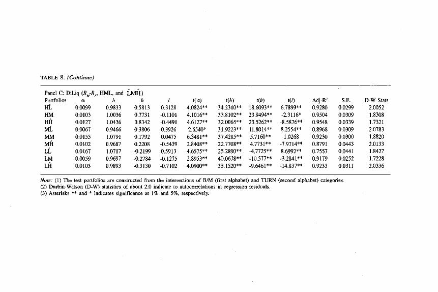
TABLE 8. (Continue)

Panel C: DiLiq (R.-R" HML, and LMil) Portfolios a b h t(a) t(b) t(h) t(l) Adj-R' S.E. D-W Stats IlL 0.0099 0.9833 0.5813 0.3128 4.0824*' 34.2310** 18.6093** 6.7899** 0.9280 0.0299 2.0052 HM 0.0103 1.0036 0.7731 -0.1101 4.1016** 33.8102** 23.9494** -2.3116* 0.9504 0.0309 1.8308 Hfl 0.0127 1.0436 0.8342 -0.4491 4.6127** 32.0065** 23.5262** -8.5876** 0.9548 0.0339 1.7321 ML 0.0067 0.9466 0.3806 0.3926 2.6540* 31.9223** 11.8014** 8.2554** 0.8968 0.0309 2.0783 MM 0.0155 1.0791 0.1792 0.0475 6.3481** 37.4285** 5.7160** 1.0268 0.9230 0.0300 1.8820 MH 0.0102 0.9687 0.2208 -0.5439 2.8408** 22.7708** 4.7731 ** -7.9714** 0.8791 0.0443 2.0\33 LL 0.0167 1.0717 -0.2199 0.5913 4.6575** 25.2890** -4.7725** 8.6992** 0.7557 0.0441 1.8427 LM 0.0059 0.9697 -0.2784 -0.1275 2.8953** 40.0678** -10.577** -3.2841** 0.9179 0.0252 1.7228 LH 0.0103 0.9893 -0.3130 -0.7102 4.0900** 33.1520** -9.6461** -14.837** 0.9233 0.0311 2.0336

Note: (1) The test portfolios are constructed from the intersections of B/M (first alphabet) and TURN (second alphabet) categories. (2) Durbin~Watson (D~W) statistics of about 2.0 indicate to autocorrelations in regression residuals. (3) Asterisks ** and * indicates significance at 1 % and 5%, respectively.

The Role of llliquidity Risk Factor 93

in Malaysian equity market is by no means unique. Similar results are also documented the United States (Chollete 2004) and in Australia (Chan & Faff 2005) and more so in emerging markets. In a study on the issue of liquidity in 48 countries, Dey (2005) found a positive, significant relationship between returns and TURN and such relationships are confined to emerging markets. The implication of positive return-TURN relationship is that it translates into

negative LMH. Earlier, Rouwenhorst (1999) found that his measure of

liquidity (HML which is the opposite of LMH) reports positive monthly values ranging from 0.11 to 1.84% in 60% of 20 emerging countries he studied. In the same study, the HML for Malaysian equity market is 0.32%. According to Pastor and Stambaugh (2003), this phenomenon reflects the behavior of investors during period when liquidity is under pressure due to events such as economic crisis. A sudden deterioration in liquidity creates a pressure strong enough to make investors to sell off their stocks at lower prices. Similarly, investors' concern about increasing cost of liquidating their assets causes them to be more receptive of lower returns. Consistent with Pastor and Stambaugh's (2003) explanation, this study finds that the

deepest trough in LMH line is during the period of 1998 to 2000 which coincides with the Asian crisis.

CONCLUSIONS

This study investigates the role of illiquidity risk factor in asset pncmg model by adopting volume-based liquidity measures. It employs monthly and yearly data of 230 to 480 companies listed on the Main Board of Bursa Malaysia for the period of 18 years from January 1987 to December 2004. The preliminary results from univariate regressions provide initial but important support for the hypothesis that illiquidity risks are priced. Not

only are the slopes of the 6 alternative measures of LMH almost consistently

significant, used alone the LMH fonned from TURN explain 30 to 36 percent of variations in stock returns.

The importance of illiquidity risks is somehow weakened when tested in multifactor models to explain returns on MEIBM test portfolios. When the multifactor models are tested on MEITURN and BMITURN test portfolios, the

role of LMH improves rather substantially even though still inferior to 5MB

and HML. The improvement is slightly more obvious when LMH is incorporated in DiLiq rather than in SiLiq. More importantly about the role

of illiquidity risk (LMH) is that it does work to improve the goodness-offits of Fama-French model. This is particularly obvious in tests on returns on BMrrURN test portfolios where DiLiq turns out to be the dominant model


in the sense that it generates the highest average adjusted R' as well highest adjusted RZ in all portfolios.

In the meantime, it is also important to note that even though the threefactor models improve the levels of goodness-of-fits of CAPM substantially, none including Fama-French model manages to reduce the alphas (a) to zero. This finding suggests at least three possibilities, (i) the existence of omitted risk factors in the tested multifactor models, (ii) the presence of undiversified firm specific risks, and (iii) the influence of abnormal February returns in this market (Ruzita & Dwipraptono 2006). One way that future

studies could address the first possibility is by incorporating LMH as an additional factor in a manner similar to Chollete (2004), Chan and Faff (2005), and Miralles and Miralles (2005). This is particularly true considering the consistently significant role of 5MB and HML regardless of which multifactor models they are considered in. The second possibility is quite high given that for quite a number of years, especially the earlier study period, the number of components stocks is less than that required to form well-diversified portfolios. Future studies should include more shares to ensure sufficient stocks to form well-diversified test portfolios. The third possibility of February effect may be addressed in future studies by excluding the February returns from the return series or by controlling February returns using a dummy variable.

But the more reliable check on the inferences about the tested models is their effectiveness to explain returns on portfolios formed on variables that are not involved in forming the explanatory factors (Fama & French 1996a). To be more meaningful, the variables should be ones that previously have been associated with CAPM anomalies such as price to earning ratio, return momentum, and dividend yield. This is because the ability to explain such anomalies is an acid test to any asset pricing model. In so far as the results of this study are concern, there is an important investment implication in that investors in this equity market should be concerned not only on market risk but also firm-specific risks, particularly size, growth potential, and the illiquidity. More specifically, investors in Malaysian equity market should require higher returns for holding equity investment in smaller size, weaker financial condition, and high turnover firms.

REFERENCES

Acharya V.v. & Pedersen, L.H. 2005. Asset pricing with liquidity risk. Journal of Financial Economics 77:375-410.

Ali, A., Hwang, L.S. & Trombley, M.A. 2003. Arbitrage risk and the book-to-market anomaly. Journal of Financial Economics 69:355-373.

Amihud, Y. 2002. Illiquidity and stock returns: Cross-section and time-series effects. Journal of Financial Markets 5(1):31-56.


Amihud, Y. & Mendelson, H. 1986. Asset pricing and the bid-ask spread. Journal of Financial Economics 17:223-249.

Bali, T.G. & Cakici, N. 2004. Value at risk and expected stock returns. Financial Analyst Journal: 57-73.

Bartholdy, J. & Peare, P. 2005. Estimation of expected return: CAPM vs Fama and French. International Review of Financial Analysis 14(4):407-427.

Bekaert, G., Harvey, C.R, & Lundblad, C. 2005. Liquidity and expected returns: lessons from emerging markets. Working Paper No. 690 presented at annual EFA conference 2003. (on-line) (24 May 2005).

Black, E 1972. The capital market equilibrium with restricted borrowing. Journal oj Business 45:444-455.

Black, E, Jensen, M.C., & Scholes, M. 1972. The capital asset pricing model: some empirical tests. In Jensen, M.e. (eds). Studies in the theory of capital markets. New York: Praeger.

Brennan, M., Chordia, T., & Suhrahmanyam, A. 1998. Alternative factor specifications, security characteristics, and the cross-section of expected stock returns. Journal of Financial Economics 49:345-373.

Brigham, E.P., Gapenski, L. & Ehrhardt, M.e. 1999. Financial Management: theory and practice (9th Ed). Fort Worth: The Dryden Press.

Chan, H.W. & Faff, R.W. 2003. An investigation on the role of liquidity in asset pricing: Australian evidence. Pacific-Basin Finance Journal 11 :555-572.

Chan, H.W. & Faff, R.W. 2005. Asset pricing and illiquidity premium. Financial Review 40:429-458.

Chollete, L. 2004. Asset pricing implications of liquidity and its volatility. Working Paper Job Market, Colombia Business School: 1-50.

Chordia, T., Subrahmanyan, A. & Anshuman, v.R. 2001. Trading activity and expected stock returns. Journal oj Financial Economics 59:3-32.

Clare, A.D., Priestley, R. & Thomas, S.H. 1997. Is beta dead? The role of alternative estimation methods. Applied Economics Letters 4:559-562.

Daniel, K. & Titman, S. 1997. Evidence on the characteristics of cross-sectional variation in stock returns. Journal of Finance 52(1):1-33.

Daniel, K, Titman, S. & Wei, K.e.J. 2001. Explaining the cross-section of stock returns in Japan: factors or characteristics. Journal of Finance 56(2):743-766.

Datar, T.v., Naik, N. & Radcliffe, R. 1998. Liquidity and stock returns: an alternative test. Journal oj Financial Markets 1:203-219.

Davis, lL., Fama, E.P. & French, K.R. 2000. Characteristics, covariances, and average returns: 1929 to 1997. Journal of Finance 55(1):389-406.

Dey, M. 2005. Turnover and return in global stock markets. Emerging Markets Review 6(1):45-67.

Drew, M.E. & Veeraraghavan, M. 2002. A closer look at the size and value premium in emerging markets: evidence from the Kuala Lumpur Stock Exchange. Asian Economic Journal 16(4):337-351.

Drew, M.E. & Veeraraghavan, M. 2003. Beta, firm size, book-to-market equity and stock returns. Journal oj Political Economy 8(3):354-379.

Fama, E.F. 1998. Determining the number of priced state variables in the ICAPM. Journal of Financial and Quantitative Analysis 33(2):217-231.

Fama, E.F. & French, K.R. 1992. The cross-section of expected stock returns. Journal oj Finance 47(2):427-465.

96 Jurnai Pengurusan 26

Fama, E.P. & French, K.R. 1993. Common risk factors in the returns on bonds and stocks. Journal of Financial Economics 33:3-56.

Fama, E.F. & French, K.R. 1996a. Multifactor explanations of asset pricing anomalies. Journal of Finance 51(1):55-84.

Fama, E.E & French, K.R. 1996b. The CAPM is wanted, dead or alive. Journal of Finance 51(5):1947-1958.

Foster. ED., Smith, T, & Whaley, R.E. 1997. Assessing goodness-of-fit of asset pricing models: the distribution of the maximal R2. Journal of Finance 52(2): 591-607.

Hameed, A. & Ting, S. 2000. Trading volume and short-horizon contrarian profits: evidence from the Malaysian market. Pasific-Basin Finance Journal 8: 67-84.

Hodrick, R.J. & Zhang, X. 2001. Evaluating the specification errors of asset pricing models. Journal of Financial Economics 62:327-376.

Jaganatban, R. & Wang, Z. 1996. The conditional CAPM and the cross-section of expected returns. Journal of Finance 51(1):3-53.

Keown, A., Scott, D, & Martin, J. 1996. Basic Financial Management (7 th Ed.). New Jersey: Prentice Hall.

Ku, K-P. & Lin W.T. 2002. Important factors of estimated return and risk: the Taiwan evidence. Review of Pacific Basin Financial Markets and Policies 5(1): 71-92.

Lesmond, D.A. 2005. Liquidity of emerging markets. Journal of Financial Economics 77:411-452.

Lintner, J. 1965. The valuation of risk assets and the selection of risky investments in stock portfolios and capital budgets. Review of Economics and Statistics 47: 13-37.

Liu, W. 2004. Liquidity premium and a two-factor model. Working paper No. 2678 presented at EFA Maastricht Meeting. (on-line) (July 2004).

Lo, A.W. & Wang, J. 2001. Trading volume: implications of an intertempora1 capital asset pricing model. Working paper of MIT Sloan. (on-line) (6 November 2001).

Maddala, O.S. 2001. Introduction to econometrics (3rd Ed). Chichester: John Wiley & Sons.

Markowitz, H. 1952. Portfolio selection. Journal of Finance 7(1):77-91. Merton, R.C. 1973. An intertemporal capital asset pricing model. Econometrica 41

(5):867-887. Miralles, J.L. & Miralles, M.M. 2005. The role of an illiquidity risk factor in asset

pricing: empirical evidence from the Spanish stock market. Quarterly Review of Economics and Finance: 1-14.

Moosa, LA. & AI-Lougbani, N.E. 1995. Testing the price-volume relation in emerging Asian stock markets. Journal of Asian Economics 6(3):407-422.

Pastor, ? & Stambaugh, R.F. 2003. Liquidity risk and expected stock returns. Journal of Political Economy 111(3):642-685.

Ross, S.A. 1976. The arbitrage theory of capital asset pricing. Journal of Economic Theory 13:341-360.

Rouwenhorst, K.G. 1999. Local returns factors and turnover in emerging markets. Journal of Finance 54(4):1439-1464.

Ruzita Abdul-Rahim & Dwipraptono Agus Harjito. 2006. Seasonality in equity markets: new evidence from four emerging markets. Jurnal Ekonomi Pembangunan 11(1):61-77.


Sharpe, W.E 1964. Capital asset prices: a theory of market equilibrium under conditions of risk. Journal of Finance 19(3):425-442.

Spiegel, M. & Wang, X. 2005. Cross-sectional variation in stock returns: liquidity and idiosyncratic risk. Working paper No. 05-13 of Yale ICF. (8 June 2005).

Stickel, S.E. & Verrecchia, R.E. 1994. Evidence that trading volume sustains stock price changes. Financial Analyst Journal 50(6):57-67.

Ruzita Abdul Rahim School of Business Management Faculty of Economics and Business Universiti Kebangsaan Malaysia 43600 UKM Bangi, Selangor D.E. Malaysia

The Role of Illiquidity Risk Factor In Asset Pricing ...journalarticle.ukm.my/8075/1/834-1591-1-SM.pdf · Jurnal Pengurusan 26(2007) 67-97 The Role of Illiquidity Risk Factor In Asset

Documents