TH¨SE UNIVERSITE DE PAU ET DES PAYS DE LADOUR cole doctorale des sciences exactes et leurs applications PrØsentØe et soutenue le 28 novembre 2019 par Arthur BLOUIN pour obtenir le grade de docteur de lUniversitØ de Pau et des Pays de lAdour SpØcialitØ : Sciences de la Terre Formation de boue partir de sØdiments stratifiØs dans un contexte de volcanisme de boue: le rle du gaz MEMBRES DU JURY RAPPORTEURS Joe CARTWRIGHT Professeur / University of Oxford Achim KOPF Professeur / University of Bremen EXAMINATEURS Lies LONCKE Matre de ConfØrence / UniversitØ Perpignan Via Domitia RØgis MOURGUES Professeur / Le Mans UniversitØ Francis ODONNE Professeur / UniversitØ de Toulouse 3 INVITE Patrice IMBERT Chercheur / Total Pau DIRECTEURS Jean-Paul CALLOT Professeur / UniversitØ de Pau et des Pays de lAdour Nabil SULTAN Chercheur / Ifremer

Welcome message from author
This document is posted to help you gain knowledge. Please leave a comment to let me know what you think about it! Share it to your friends and learn new things together.
Transcript

THÈSE UNIVERSITE DE PAU ET DES PAYS DE L�ADOUR
École doctorale des sciences exactes et leurs applications
Présentée et soutenue le 28 novembre 2019
par Arthur BLOUIN
pour obtenir le grade de docteur de l�Université de Pau et des Pays de l�Adour
Spécialité : Sciences de la Terre
Formation de boue à partir de sédiments stratifiés dans un contexte de volcanisme de boue:
le rôle du gaz
MEMBRES DU JURY RAPPORTEURS � Joe CARTWRIGHT Professeur / University of Oxford � Achim KOPF Professeur / University of Bremen
EXAMINATEURS � Lies LONCKE Maître de Conférence / Université Perpignan Via Domitia � Régis MOURGUES Professeur / Le Mans Université � Francis ODONNE Professeur / Université de Toulouse 3
INVITE � Patrice IMBERT Chercheur / Total Pau
DIRECTEURS � Jean-Paul CALLOT Professeur / Université de Pau et des Pays de l�Adour � Nabil SULTAN Chercheur / Ifremer

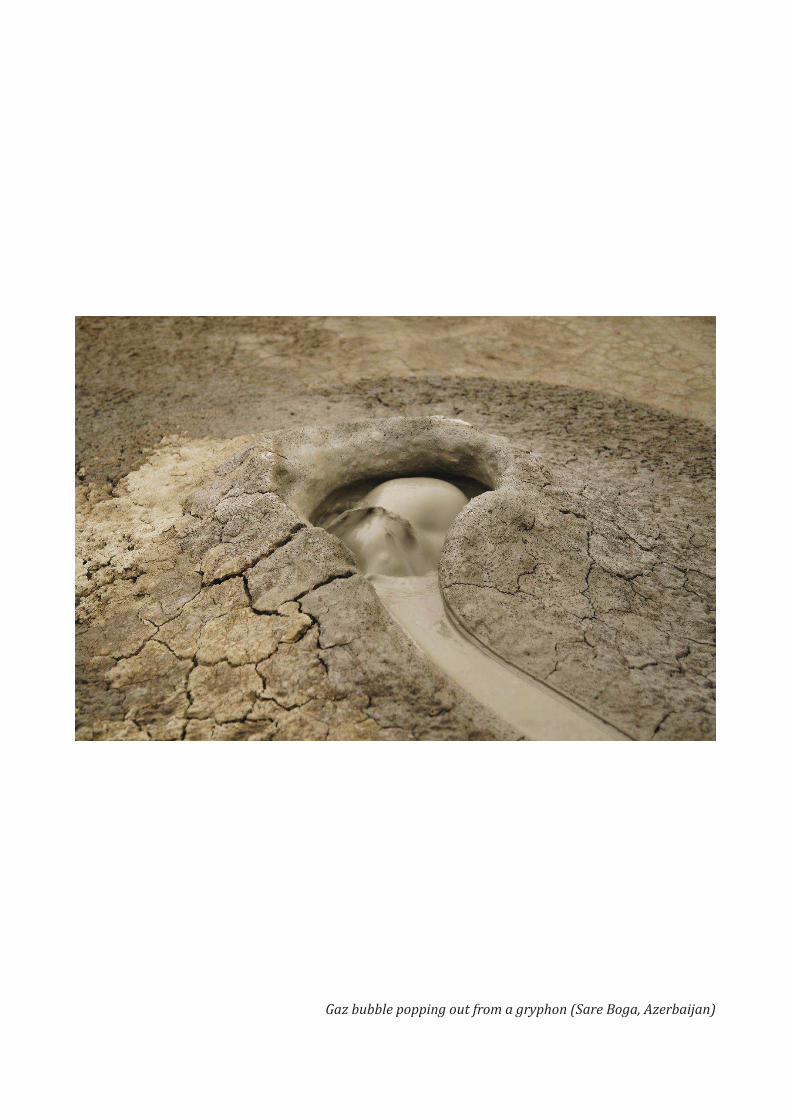
Gaz bubble popping out from a gryphon (Sare Boga, Azerbaijan)


Page | i
Acknowledgments/Remerciements
I would like to start by thanking all the jury members who accepted and did me the honor to read and
examine my manuscript: Achim Kopf, Joe Cartwright, Lies Loncke, Régis Mourgues and Francis Odonne.
I really hope that you will enjoy reading this work.
Je voudrais ensuite remercier la triforce de cette thèse, soit mes trois encadrants. Merci à Nabil pour
ton efficacité, ta disponibilité malgré ton rôle de responsable d�unité et tes « dead lines ». Au début c�est un
peu stressant, on se dit qu�on ne finira jamais les trois ans en restant sain d�esprit, mais in fine on s�y fait, on
prend le rythme et c�est très efficace. Merci pour les conversations très ouvertes que nous avons pu avoir
ensemble que ce soit sur de la science ou sur d�autres sujets. Encore désolé pour toutes les fois où tu as du
corriger mes erreurs de calculs. Quoiqu�il en soit, grâce à toi, je peux dire que je maîtrise beaucoup mieux la
géotechnique, en particulier dans le domaine marin ce qui était nouveau pour moi. Jean-Paul, merci
énormément pour ta disponibilité. Tu as toujours répondu présent pour la moindre chose dont j�avais besoin.
Merci pour avoir toujours proposé de nouvelles idées et d�avoir toujours su m�expliquer des concepts qui me
paraissaient à première vue obscurs. Merci pour m�avoir souhaité la bienvenue à Pau avant même le début
de mon contrat, et d�avoir su me mettre à l�aise dès le début en me spécifiant toute fois tes attentes sur cette
thèse. Patrice, merci pour ta disponibilité, ta bonne humeur et de m�avoir appris toutes tes astuces de vieux
pirate de l�interprétation sismique. Grâce à toi, j�arrive dans le monde du travail avec de solides compétences.
Cela a été un réel honneur d�être ton dernier étudiant en thèse avant ton départ de Total. Merci de m�avoir
guidé et pour les bons moments passés ensemble sur les trois grandes conférences où j�ai présenté mes
travaux. Merci aussi pour m�avoir fait découvrir les c�urs de canard : je ne pense pas que j�aurais goûté cela
un jour sans cette invitation à diner. Enfin, merci à vous trois pour avoir dirigé et encadré cette thèse dans
des styles certe très différents (Patrice le poète et ses concepts, Nabil l�ingénieur et ses calculs et Jean-Paul
l�encyclopédie humaine) mais toujours dans la bonne humeur. Je crois que je ne pouvais pas mieux tomber.
Cette thèse se fait dans le cadre d�un partenariat entre Ifremer et Total. Aussi merci à ces deux
entreprises d�avoir cru en ce travail et de m�avoir fait confiance pour mener à bien cette recherche. Merci
également pour les financements et les moyens matériels et humains déployés pour le bon déroulement de
mon travail.
Merci à l�Université de Pau et des Pays de l�Adour de m�avoir accueilli comme étudiant et d�avoir fait
des concessions afin de limiter mes déplacements Brest-Pau. Merci à toutes les personnes rencontrées là-
bas pour l�intérêt porté sur mon travail et les discussions que j�ai pu avoir avec plusieurs d�entre vous à
différentes occasions.
Merci à l�équipe de choc pour le terrain en Azerbaïdjan en 2017. Merci à Francis Odonne et Patrice
Imbert de m�avoir proposé cette mission qui m�a permis de toucher du doigt (et du bras) mon sujet d�étude.

Acknowledgments/Remerciements
Page | ii
Merci à Matthieu Gertauda pour ces bons moments passés sur le terrain, et les balades dans Bakou. Merci
pour le T-Shirt, je le porte fièrement au travail. Special thanks to Orhan Abbasov and Elnur Baloglanov for
their help and kindness. You were very friendly to us and I hope we will meet again soon. Merci au moustique
mutant qui m�a permis de connaître le système hospitalier de Haciqabul, sans toi l�aventure n�aurait pas été
la même.
Merci aux équipes et aux collègues de Total. En particulier merci à toute l�équipe R&D pour l�accueil et
les nombreuses discussions. Remerciements stout particulier à Claude Gout qui a toujours cru dans le travail
de Patrice (malgré les risques d�éboulements dans son bureau) et par extension dans mon travail. Toujours
prêt à discuter, tu poses toujours la question qui permet d�aller plus loin. Merci à Jérémie Gaillot qui a pris
du temps afin de m�expliquer les résultats de mes analyses biostratigraphiques, et à Claire Fialips pour sa
participation dans les analyses minéralogiques et leur interprétation. Merci à toute l�équipe de la carothèque
pour avoir déballé et remballé les carottes et cuttings je ne sais combien de fois. Merci à Cathy qui m�a
souvent aidé avec mes démarches en interne à Total. Merci aussi à Fugro, sans qui, à deux mois près, je
n�aurais pas eu accès aux sédiments d�Absheron.
Merci à toutes les personnes cotoyées à Ifremer. En particulier, merci beaucoup à Bruno Marsset
toujours à l�écoute y compris des étudiants. Merci pour ton soutien et de m�avoir rappelé quelques fois que
j�avais des congés pour une raison. Merci à Mickael Rovere pour m�avoir formé et passé du temps avec moi
sur les oedomètres. Merci à Mickael Roudaut et à Ronan Apprioual pour la construction de la cellule d�essai
et sa maintenance sans laquelle cette thèse n�aurait pas pu avoir lieu. Merci particulièrement à Mickael pour
avoir passé une journée entière avec moi pour installer un système d�évacuation pour le CO2. Merci à Livio,
Vincent, Sébastien, Shane et Stephan pour les discussions et vos conseils qui m�ont permis d�améliorer mon
travail. Merci à Pauline pour ton aide qui m�a permis de garder un ordinateur opérationel durant ces trois
ans (et c�était pas gagné). Merci à Alison, Sylvia et Babette pour m�avoir aidé plusieurs fois à m�en sortir avec
mes ordres de mission (désolé pour les casses-têtes). Thank you Alison for correcting my English. Merci à
Hélène et à Marie-Odile pour m�avoir permis de réaliser avec vous une vidéo sur les volcans de boue. La vidéo
sur les hydrates n�a pas été rattrapée, je vais donc songer à m�inscrire à Twitter... Enfin un merci tout
particulier à Frauke, Louis et Tania qui m�ont donné goût à la géologie marine dès le troisième.
Merci à tous les amis rencontrés pendant cette thèse, au gré de mes déplacements.
A Pau, je voudrais remercier tout particulièrement Salomé. Grâce à toi, j�ai intégré une super bande
de potes, et même si nous venons tous d�endroits différents, vous resterez pour moi « les Palois ». Merci à
Simon, Johann, Carl, Kasim, Amine et Veronica les expatriés du bâtiment EA. Merci à tous « les Palois »
(désolé je ne vous cite pas tous) pour tous ces supers moments dans le Sud-Ouest pendant un an à base
randonnées, de balade, de surf, de ski, de bonnes bouffes et de soirées. Merci à vous tous d�avoir été là dans
les bons et les mauvais moments. Merci à Samy, mon moniteur de ski pour une journée : la prochaine fois je

Acknowledgments/Remerciements
Page | iii
ne tomberai pas dans le tapis roulant, c�est promis. Antoine, merci d�être aussi râleur que moi, je me sentais
moins seul ! Merci à Alexandre (Dr. Pichat) et Etienne (Dr. Legeay) pour tous les bons conseils de vieux
thésards ainsi que pour les pauses que vous vous accordiez lorsque j�étais de passage à l�UPPA.
A Brest mêm�, merci à la bande de copains de toujours, pour m�avoir apporté des moments de
décompression et de fun si précieux surtout rendu en fin de thèse. Big Up à Maud, Xavier et Julien qui m�ont
fait reprendre le sport : ça m�a permis de souffler et de limiter ma prise de circonférence. Merci aussi à mes
amis et collègues thésards et ex-stagiaires pour tous ces bons moments passés à Ifremer et en-dehors. Plus
particulièrement une grosse pensée pour Farah et Déborah qui ont supporté ces deux dernières années mes
grognements et sautes d�humeur à chaque fois que « Word a cessé de fonctionner » (ou pour toute autre
raison d�ailleurs). Merci à Aurélien et Maude pour cette journée de pêche à pied mémorable ! Merci
également à Alexandra Pierron, qui est ma première stagiaire. Tu as fait du super boulot, et ça m�a
énormément aidé (Cf Chapitre 5).
A Nancy, merci à tous mes anciens amis de la promotion 2016 de l�ENSG. Je rêvais de faire cette école,
mais en fait c�était encore mieux ! Merci à Brieuc et Mathieu, mes anciens colocataires, avec qui on a passé
de supers moments, récemment ou non, et surtout avec qui j�ai appris à rédiger des rapports de terrain aux
petits oignons. Je pense que cette compétence m�a été fort utile. Merci aussi à Yves Géraud et Jean-Marc
Montel pour le soutien qu�ils m�ont apporté pendant l�école mais aussi depuis l�école.
Enfin, merci à ma famille et belle-famille ains qu�à tous les proches qui m�ont accompagné et soutenu
pendant toutes mes études. Merci particulier à Françoise et Dominique qui m�ont donné le goût du voyage.
Gracias a la familia y amigos de Mexico que siempre estuvieron al pendiente de mis avances. En particulier,
merci à ma mère pour m�avoir toujours poussé à être curieux et pour m�avoir donné le virus de la recherche.
Merci d�avoir toujours cru dans mes capacités et de m�avoir poussé (¡ a chanclazos !) à aller jusqu�au bout en
faisant cette thèse. Merci à mon père sans qui ma vocation de « casseur de cailloux » ne serait pas apparue
si tu ne m�avais pas fait visiter le musée de paléontologie à Paris. Merci à Axel, mon petit frère, pour le jeune
homme intelligent, responsable et bon que tu es devenu. A toi maintenant d�aller au bout de tes rêves et de
tes projets. Enfin, merci à Maud, toi qui plus que tous, a eu à supporter mon stress, mes humeurs et ma
fatigue. Tu as su me canaliser et tu m�as accompagné depuis le tout début (en prépa), en passant par ces 4
années de distance (we did it !), jusqu�à Brest où tu as en plus dû apprendre à vivre tous les jours avec mon
côté maniaque. Toi aussi tu as fait ton bonhomme de chemin ! Je ne suis définitivement plus un « petit
étudiant » comme tu avais l�habitude de me dire.
Merci Thanks Gracias T ! kkür

Acknowledgments/Remerciements
Page | iv

Acknowledgments/Remerciements
Page | v
First contact with mud. I did not keep my hands clean very long (sorry Mum)

Acknowledgments/Remerciements
Page | vi
Page | vii
Table of contents
Acknowledgments/Remerciements ............................................................ i
Table of contents ...................................................................................... vii
List of Figures ........................................................................................... xiii
List of tables .......................................................................................... xxvii
List of equations .................................................................................... xxix
Chapter 1: Scientific Background ........................................................... 1
1. Introduction (English) .......................................................................................... 5
1. Introduction (Français) ........................................................................................ 9
2. Significance of mud volcanism .......................................................................... 13
2.1. Mud volcano definition and lexicon .................................................................................... 13
2.2. Occurrence and geological setting for mud volcanism ....................................................... 15
2.3. Mud composition and origin of the different constitutive elements.................................. 17
2.4. Morphology and architecture of a mud volcano system .................................................... 19
2.4.1. Source domain ........................................................................................................................... 20
2.4.2. Intrusive domain ........................................................................................................................ 21
2.4.3. Extrusive domain ....................................................................................................................... 23
2.4.4. Roof domain .............................................................................................................................. 25
2.5. Triggers for mud genesis and drivers of sediment remobilization ...................................... 26
2.5.1. Overpressure generation ........................................................................................................... 26
2.5.2. The role of methane .................................................................................................................. 31
2.5.3. Density inversion ....................................................................................................................... 32
3. Goal and scope of this research ........................................................................ 35
3. But et cadre de ce travail de recherche ............................................................. 39
4. Thesis outline .................................................................................................... 43
4. Plan de la thèse ................................................................................................. 45

Contents
Page | viii
Chapter 2: Study Area, Data and Methodology ................................... 47
1. Study Area ......................................................................................................... 51
1.1. South Caspian Basin ............................................................................................................. 51
1.1.1. Geodynamics and present tectonic background ....................................................................... 51
1.1.2. Paleogeography and regional stratigraphy ............................................................................... 56
1.1.3. Oil & gas potential and mud volcanism ..................................................................................... 60
1.2. Absheron fold: gas-condensate field and geohazards ........................................................ 63
2. Data acquisition and location ............................................................................ 64
2.1. 3D seismic survey................................................................................................................. 64
2.2. Geotechnical and geophysical survey.................................................................................. 65
2.2.1. Geophysical dataset .................................................................................................................. 65
2.2.2. Coring and in situ mechanical measurements .......................................................................... 66
2.3. Exploration wells .................................................................................................................. 66
2.3.1. Gamma-ray and caliper logs ...................................................................................................... 67
2.3.2. Sonic logs ................................................................................................................................... 67
2.3.3. Density log ................................................................................................................................. 68
2.3.4. Neutron logs .............................................................................................................................. 68
2.3.5. Resistivity logs ........................................................................................................................... 68
2.3.6. Lithology .................................................................................................................................... 69
2.3.7. Formation pressure logs, rock strength, temperature and gas out .......................................... 70
3. Methods ............................................................................................................ 72
3.1. Seismic interpretation ......................................................................................................... 72
3.2. Sediment analysis ................................................................................................................ 72
3.2.1. Mineralogy ................................................................................................................................. 73
3.2.2. Biostratigraphy .......................................................................................................................... 74
3.2.3. Grain-size distribution ............................................................................................................... 74
3.2.4. Mechanical properties of sediments ......................................................................................... 75
3.3. Well data interpretation ...................................................................................................... 81
3.4. Numerical modeling............................................................................................................. 82
3.4.1. 1D sedimentation and pore pressure accumulation ................................................................. 82
3.4.2. Two-dimensional transient-diffusion process: Darcy�s and Fick�s laws .................................... 82
3.4.3. P-wave velocity with gas saturation .......................................................................................... 83
3.4.4. Fluid mud dynamics: modelling approach ................................................................................. 84
4. Conclusion ......................................................................................................... 85

Contents
Page | ix
Chapter 3: Evolution model for the Absheron mud volcano: from in situ
observations to numerical modeling ................................................... 87
1. Introduction ...................................................................................................... 91
2. Regional Setting ................................................................................................ 92
3. Materials and methods ..................................................................................... 94
3.1. Seismic data ......................................................................................................................... 94
3.2. Sediment cores and geotechnical analysis .......................................................................... 96
3.2.1. Sample collection....................................................................................................................... 96
3.2.2. Mineralogical and biostratigraphic analysis of the mud ........................................................... 97
3.2.3. Geotechnical analysis of the mud ............................................................................................. 98
3.3. In situ well data and hydraulic conductivity calculations .................................................... 99
3.4. Numerical modeling: sedimentation, transient pore pressure and gas diffusion ............ 100
3.4.1. 1D sedimentation and pore pressure accumulation ............................................................... 100
3.4.2. Two-dimensional transient-diffusion process: Darcy�s and Fick�s laws .................................. 101
3.4.3. Hydrofracturing ....................................................................................................................... 102
4. Results ............................................................................................................. 102
4.1. Geomorphological investigation of the Absheron mud volcano....................................... 102
4.2. Physical, sedimentological and geotechnical properties of the mud................................ 115
4.3. In situ lithology, temperature and excess pore-pressure derived from in situ well data . 119
4.4. Numerical calculations of transient pore pressure and methane diffusion...................... 122
4.4.1. 1-D modeling ........................................................................................................................... 122
4.4.2. 2-D modeling ........................................................................................................................... 123
5. Discussion ....................................................................................................... 126
5.1. What is the stratigraphic source of the mud? ................................................................... 126
5.2. How do the field pore pressure measurements compare to the model? ......................... 128
5.3. How does methane diffusion interact with excess pore pressure accumulation? ........... 129
5.4. What is the most plausible sequence for the formation of the Absheron mud volcano .. 130
5.5. Limits and perspectives of the study ................................................................................. 133
6. Conclusions ..................................................................................................... 134
Contents
Page | x
Chapter 4: Sediment damage caused by gas exsolution: a key
mechanism for mud volcano formation ............................................ 137
1. Introduction .................................................................................................... 141
2. State of the art on gassy sediments ................................................................ 142
2.1. Definition of gassy sediments ............................................................................................ 142
2.2. Occurrence and relevance of gassy sediments ................................................................. 144
2.3. Creating gassy sediments during laboratory testing ......................................................... 146
2.4. Hydro-mechanical properties of gassy sediments ............................................................ 147
2.4.1. Gassy sediment acoustic response .......................................................................................... 147
2.4.2. Gassy sediment compressibility .............................................................................................. 148
2.4.3. Gassy sediment permeability .................................................................................................. 149
2.4.4. Sediment damage due to gas exsolution ................................................................................ 150
2.4.5. Effect of gas bubbles on the sediment shear strength ............................................................ 151
3. Experimental testing ....................................................................................... 151
3.1. Properties of the tested soil and sample preparation ...................................................... 151
3.2. Experimental set-up and calibration ................................................................................. 154
3.3. Testing program ................................................................................................................. 158
4. Results ............................................................................................................. 159
5. Synthesis of experimental results .................................................................... 167
5.1. Fractures, sediment damage and remolding ..................................................................... 167
5.2. Effect of gas exsolution on P-wave velocity ...................................................................... 169
5.3. Effect of degree of gas saturation on sediment compressibility ....................................... 170
5.4. Hydraulic conductivity versus degree of gas saturation ................................................... 171
5.5. Preconsolidation pressure evolution with degree of gas saturation ................................ 172
6. Discussion ....................................................................................................... 173
6.1. Fracture size and number: main controlling factors ......................................................... 173
6.2. Gas exsolution/expansion: a permanent P-wave velocity attenuation? .......................... 174
6.3. Gas exsolution/expansion effects on sediment compressibility ....................................... 175
6.4. Gas exsolution/expansion effects on sediment permeability ........................................... 176
6.5. Gas exsolution/expansion effects on preconsolidation pressure and the consequence in
terms of shear strength ............................................................................................................ 177
7. Conclusions ..................................................................................................... 178

Contents
Page | xi
Chapter 5: From stratified sediments to fluid mud generation ........... 181
1. Introduction .................................................................................................... 185
2. Material and methods ..................................................................................... 186
2.1. Mud generation ................................................................................................................. 186
2.2. Mud ascent ........................................................................................................................ 188
3. Results ............................................................................................................. 190
3.1. Mud generation ................................................................................................................. 190
3.1.1. One-dimensional sedimentation and pore pressure accumulation ........................................ 190
3.1.2. Two-dimensional transient-diffusion processes, gas exsolution and damage ........................ 191
3.2. Mud ascent ........................................................................................................................ 199
3.2.1. Code1 v1 .................................................................................................................................. 200
3.2.2. Code1 v2 .................................................................................................................................. 203
3.2.3. Extrapolation to realistic viscosities: 1D calculations .............................................................. 206
4. Discussion ....................................................................................................... 208
4.1. Synthesis of the main results ............................................................................................. 208
4.2. Overpressure, hydrofracturing and gas exsolution: from stratified sediments to fluid mud
.................................................................................................................................................. 209
4.3. Mud extrusion resulting from density-inversion driven by gas exsolution ....................... 211
4.4. Towards a quantitative formation model for the Absheron mud volcano ....................... 213
5. Conclusion ....................................................................................................... 219
Chapter 6: Synthesis, conclusions and perspectives ........................... 221
1. Introduction .................................................................................................... 223
2. The formation of a mud volcano: a close relationship between gas and
overpressure ....................................................................................................... 223
2.1. The source of the Absheron Mud Volcano: intrinsic factors and external parameters .... 223
2.2. Mud generation through gas exsolution ........................................................................... 225
2.3. Integrated numerical models: mud generation and remobilization under geological
conditions ................................................................................................................................. 226
3. Possible further improvements ....................................................................... 228
3.1. Dataset ............................................................................................................................... 228
3.2. Experimental study ............................................................................................................ 229

Contents
Page | xii
3.3. Numerical modeling........................................................................................................... 230
4. Scientific implications and perspectives .......................................................... 231
Chapitre 6 : Synthèse, conclusions et perspectives ............................ 233
1. Introduction .................................................................................................... 235
2. La formation d�un volcan de boue : une relation étroite entre le gaz et la
surpression ......................................................................................................... 235
2.1. La source du volcan de boue d�Absheron : facteurs intrinsèques et paramètres extérieurs
.................................................................................................................................................. 235
2.2. La génération de boue par exsolution de gaz.................................................................... 237
2.3. Modèles numériques intégrés : génération et remobilisation de la boue dans les
conditions géologiques ............................................................................................................. 239
3. Axes d�amélioration ........................................................................................ 241
3.1. Le jeu de données .............................................................................................................. 241
3.2. Etude expérimentale ......................................................................................................... 242
3.3. Modélisation numérique ................................................................................................... 243
4. Implications scientifiques et perspectives de cette étude ............................... 244
References ............................................................................................. 247
Appendix 1: Additionnal testing results ................................................. 269
Appendix 2: Published journal articles ................................................... 275

Page | xiii
List of Figures
Chapter 1
Figure 1.1: a: Google Earth 2018 3D view of the Bozdag Guzdek mud volcano (Azerbaijan) with a vertical exaggeration
of 3. This mud volcano has a basal diameter of 2 km, its crater being 500 m large and oval. Several km-long mudflows
are visible on its northern flank. b: gryphon pictured in May 2017 at the top of the Sareboga seeping site (Azerbaijan).
It shows the cm to m scale seeping sites that can be found at the top of active MVs during their dormant phase. It also
displays the different phase composing the mud: fine-grained sediments, water and gas. c-d: mud expelled from
onshore MVs in Azerbaijan. c: northern highly viscous and dry mudflow from the Koturdag MV (Azerbaijan, May 2017).
It carries among its fine-grained matrix, m-scale to cm-scale rock clasts. Sinter structures (orange) correspond to points
were gaseous methane was emitted and ignited spontaneously, heating the surrounding clay minerals. d: highly fluid
mudflow emitted from the gryphon pictured in b. The mud is saturated with water and it behaves like a fluid. Mud
flowed along the natural slope for 100 meters at least. ................................................................................................... 14
Figure 1.2: global distribution map of known mud volcanoes offshore and onshore (from Mazzini & Etiope, 2017). ..... 15
Figure 1.3: Methane carbon and hydrogen isotope diagram for mud volcanoes (from Etiope et al., 2009). ................... 18
Figure 1.4: schematic diagram of a mud volcano system, displaying its main structural domains. The features common
for most of mud volcanoes are represented and only morphological and geometrical considerations are displayed
(modified from Kirkham, 2015). ........................................................................................................................................ 19
Figure 1.5: a- seismic section across a mud volcano system in the South Caspian Basin showing a thinning of the
Maykop Formation interval interpreted as being the source layer of the mud volcano. b- Depth map of the top of the
Maykop Formation underlining a thrust. c- Thickness map of the Maykop Formation showing a depleted zone inside
the red dotted line (from Stewart & Davies, 2006). .......................................................................................................... 20
Figure 1.6: interpreted seismic section showing the bowl-shaped features at the crest of an anticline in the South
Caspian Basin, interpreted as former mud chambers (from Dupuis, 2017). Interval 2 is partially truncated by interval 3.
Interval 1 is undisturbed. The interval 4 is interpreted as being mud extrusions initially sourced in the truncated interval
2. Sediment remobilization provoked a collapse of intervals younger than the source. .................................................. 21
Figure 1.7:"a:"seismic"section"showing"the"subsiding"column"of"intruded"sediments"named"�downward"tapering"cone�"
by Stewart & Davies (2006). It is located below several biconical extrusive edifices (from Stewart & Davies (2006)). b:
coherency time slice showing the chaotic structure inside the DTC (from Stewart & Davies, 2006). ............................... 22

Contents
Page | xiv
Figure 1.8:"example"of"a"buried"mud"volcano"offshore"of"Trinidad"with"the"typical"�Christmas"tree�"morphology."This"
architecture is the result of the cyclic development of the volcanic edifice, with short eruptive periods that contrast with
the longer dormant periods when normal sedimentation dominates (from Deville, 2009). ............................................ 24
Figure 1.9: Different morphologies of MVs due to different internal processes and external forces (from Mazzini &
Etiope, 2017). (A) conical, (B) elongated, (C) pie-shaped, (D) multicrater, (E) growing diapir-like, (F) stiff neck, (G)
swamp-like, (H) plateau-like, (I) impact craterlike, (J) subsiding structure, (K) Subsiding flanks, (L) sink-hole type. ....... 25
Figure 1.10: pressure versus depth plot showing hydrostatic (Phydro) and lithostatic (Plitho) pressures. The green line is the
measured pressure. The difference between the measured pressure and hydrostatic pressure represents the
overpressure and the difference between the lithostatic and measured pressure gives the effective stress (modified
from Deming, 2002). ......................................................................................................................................................... 27
Figure 1.11: Conceptual mud volcano system model from Deville et al. (2010) showing a possible reaction chain and
processes leading to sediment remobilization and mud volcano formation. ................................................................... 33
Chapter 2
Figure 2.1: Topographic/Bathymetric map around the South Caspian Sea using the GEBCO 2014 database. The -500 m
contour line is represented and highlight the main depocenters in the Caspian Sea. The main fold and thrust belts and
reliefs delimiting the South Caspian Basin are located as well as the main river systems linked to the SCB history. The
study area is located by a purple rectangle. SCB: South Caspian Basin; CCB: Central Caspian Basin; NCB: North Caspian
Basin. ................................................................................................................................................................................ 51
Figure 2.2: Simplified tectonic map of the South Caspian area showing the main tectonic units (modified from Brunet et
al., 2003). A: Aghdarband; Ap: Absheron;A Trialet: Achara-Trialet; EO: Erevan-Ordubad; E Pontides: Eastern Pontides;
GB: Great Balkhan; Go: Gorgan; K: Karabakh; L Caucasus: Lesser Caucasus; Na: Nayband; R: Rasht; SP; Scythian
platform; TC: Terek � Caspian basin; WT: Western Turkmenia. The present SCB is delimited by the red dotted line and is
located partly onshore. ..................................................................................................................................................... 53
Figure 2.3: a: Simplified structural map of the Caspian area including GPS-derived estimations for plate velocities.
ALBZ: Alborz block; AN; Anatolian Plate; CAUC: Caucasus Plate; SCB: SCB Block (modified from Santos Betancor, 2015).
b: Map showing earthquakes of the CCB and SCB regions taken from the IRIS catalogue for the period between 1970
and 2010 and classified by depth of their hypocenters (modified from Santos Betancor, 2015). Blue dotted line marks
the oceanic crust of the SCB and the purple rectangles show the approximate location of the study area. .................... 55

Contents
Page | xv
Figure 2.4: Generalized lithostratigraphic column for the SCB. The Jurassic�Miocene sequence is known from outcrops
in eastern Caucasus, while the Pliocene and younger section were drilled in the SCB. Ages are given in million years.
The Lower PS are subdivided in Kala Suite (KAS), Under-Kirmaky Suite Sandstone (PK), Kirmaky Suite (KS), Above-
Kirmaky-Sandstone (NKP) and Above-Kirmaky Shale (NKG). The transgressive and regressive trends are those given by
Abreu & Nummedal (2007). Figure adapted and modified from Green et al., (2009) and Javanshir et al. (2015). .......... 57
Figure 2.5: schematic map of the Paleo-drainage systems during the deposition of the Productive Series (Late Miocene-
Pliocene). The possible sources of sediments are displayed as well as the location of the paleo-deltas. The purple box
shows the approximate location of the study area (modified from Smith-Rouch, 2006). ................................................ 58
Figure 2.6: HC generation and accumulation temporal chart for the Oligocene�Miocene Maykop/Diatom Total
Petroleum System in the South Caspian Basin Province. Ak-Ap: Akchagyl and Absheron intervals. The critical moment
correspond at the time when all the criteria for oil & gas generation, accumulation and preservation were present and
correspond to the Akchagyl strata deposition (from Smith-Rouch, 2006). ....................................................................... 62
Figure 2.7: Seafloor depth map extracted from the 3D seismic survey, showing the location of the other surveys and
samples used during this research. The AMV is visible as a light blue patch where the dataset is denser. Seafloor depth
is given in meters below mean sea level. The Purple rectangle shows the maximum extent of the 3D seismic survey, the
black polygon shows the extent of the multibeam echo sounder survey, and the red rectangle, the area where
backscattering image was processed. Samples are represented with different symbols depending on their type. Red
circles with crosses: exploration wells; orange circles with dots: rotary drillings and CPT measurements; blue
pentagons: piston cores from AUV survey, 2014; yellow square: box core from AUV survey, 2014; green triangles:
samples for biostratigraphy from Chevron survey, 1999. ................................................................................................. 64
Figure 2.8:"Log"data"from"well"ABX2"presented"as"an"example"of"lithology"interpretation."a:"�quick-look�"log"plotted"
during drilling operations for monitoring purposes. The main data acquired with LWD tools are the gamma-ray (GR)
signal (green) and the resistivity (shallow in blue, deep in red). These geophysical data are coupled with cuttings
analysis in order to present a preliminary lithological section. b: final composite log, with all geophysical data obtained
over a given section (GR; resistivity, shallow and deep field; sonic, DTP for P-waves and DTS for S-waves; density;
neutron). Using data from resistivity coupled with sonic, and superimposed neutron and density, it is possible to refine
the lithological log notably by precisely highlighting reservoir facies (yellow color, right column). ................................ 71
Figure 2.9: a: picture of the fall cone test apparatus, displaying the main elements. b: typical log-log diagram of the
water content versus the penetration depth, displaying the reading methods for the Atterberg limits (from Feng, 2005).
.......................................................................................................................................................................................... 75
Figure 2.10: a: picture showing one oedometer used during the study, displaying the main elements of the system. b:
typical plot for an odeometer test result after increment load and unload, displaying the consolidation curve, the

Contents
Page | xvi
swelling curve and the virgin consolidation curve. The method for calculating the preconsolidation pressure (s�P0) and
for the reading of the compression index (CC) and swelling index (CS) is also displayed. A is the maximum inflexion point
of the laboratory consolidation curve. From this point, the tangent to the curve and the horizontal line are drawn. The
bisector between these two lines gives the point B at the intersection with the virgin consolidation curve. The
horizontal coordinate of B gives s�P0. ............................................................................................................................... 77
Figure 2.11: Picture showing the main modules of the special consolidation testing. Details are given in the Chapter 4,
dedicated on the experimental testing program and results. ........................................................................................... 78
Figure 2.12: Adopted method to apply the effective medium theory of Helgerud et al. (1999) (modified from Taleb et
al., 2018). .......................................................................................................................................................................... 84
Chapter 3
Figure 3.1: A, structural map of the South Caspian region showing the main folds and faults, structural domains and
depocenters (modified from Oppo et al., 2014). B, regional interpreted deep seismic section, showing the main
subsurface structural elements with the folds above the Maykop detachment level associated in the northern part to
deeply rooted thrusts. The location of the line is shown on the left map by a black line. The red box shows the
approximate location of the Absheron structure (modified from Stewart & Davies, 2006). ............................................ 92
Figure 3.2: Seismic amplitude map of the seafloor around the Absheron mud volcano. In orange, a high amplitude
mudflow is imaged to the west of the volcano. The dark patch corresponds to the shield composing the mud volcano
itself. On the same map, the location of the different coring and drilling sites are shown. Limits and location of the 3D
seismic survey are presented on the regional map of the SCB (Figure 3.1A). Red lines indicate the location of the seismic
lines presented in Figure 3.3, Figure 3.4 and Figure 3.5. The dotted black polygone is the limit of the zoom shown
below, presenting a detailed image of the seafloor on and around the mud volcano acuired with a multi-beam echo
sounder. Orange stands for the shallower areas, green is for the deeper parts. ............................................................. 96
Figure 3.3: Uninterpreted and interpreted seismic line crossing the anticline near the two exploration wells A and B; it
was used as reference for horizon picking for this study. A deep thrust cores the Absheron anticline and another thrust,
smaller is also visible at the NNE of the section. From the thickness differences between the flanks and the crest of the
structure, we note that folding started during the Akchagyl deposition. The main growing phases are during deposition
of the Absheron Suite (A3-A1) and later during the Post-Absheron times. See Figure 3.2 for location. ......................... 103
Figure 3.4: Uninterpreted and interpreted seismic line across the active mud volcano. The first 2 km are clearly imaged
and show four seismically transparent wedges, corresponding to mudflows. A chaotic signal below can be

Contents
Page | xvii
discriminated from the blind signal and is interpreted as reworked sediments. The rooting system is blind, maybe due
to a masking effect from the low velocity mud deposits. Near the blind area, some normal faults are present between
1.5 and 3 km. A deep thrust is coring the main anticline. The activation of the mud volcano is contemporaneous to the
main folding phase (see text and Figure 3.3 for details, Figure 3.2 for location).s directly be interpreted as mudflow
deposits forming the mudvolcano edifice (green patch on Figure 3.4). Below 2 km at the center of the structure, a
seismically transparent cone goes down to 7 km. This area could reveal the masking effect of the low velocity mass
formed by the shallower mud deposits that may also be saturated with gas, preventing the acoustic signal from
propagating below. Another seismic facies can be discriminated from the blind signal: the blue patch can be described
as a chaotic signal. This area is located between the mudflows and host sediments. ................................................... 105
Figure 3.5: Uninterpreted and interpreted seismic line south of the mud volcano center. The gas blanking effect reduces
below the mudflows. The transparent and chaotic signals are still present. A bending of seismic horizons from 1.5 to 3
km is noted forming a bowl-like geometry. Horizons of the upper part of the Anhydritic Surakhany are truncated by
younger intervals as well as a 400 m thick interval in the lower part of the Upper Productive Series. Horizons recovers
their continuity and their flat geometry below 3800 m in the Productive Series. See Figure 3.2 for location. ............... 107
Figure 3.6: Applied method to channel recognition with the example of Layer 2 (Figure 3.7). A: the RMS of seismic
amplitude is calculated on layers computed between two seismic horizons (here A3 and PS1). Elongated, curved and
continuous bodies having the same RMS are potential channels. The surface location of the AMV is displayed with
dotted lines. B: interpreted layer with confirmed channel bodies in green. The red line corresponds to the zoom of
seismic section presented in C. The surface location of the AMV is displayed with dotted lines. C: zoom on a seismic
section (location displayed in B, red line) perpendicular to a potential channel recognized on A. The seismic section is
from the PSTM seismic block, and the vertical scale is given in ms TWTT (two-way travel time). At the exact location of
the elongated body, a downward bending of two horizons is visible (red dotted rectangle). This bending is local and
only affects two seismic horizons, thus, the body is interpreted as a channel. .............................................................. 108
Figure 3.7: A: interpreted section presented in Figure 3.3, displaying in green the stratigraphic interval where layers
were computed. The black dotted line highlights the Layer 29. B: examples of channels found over several layers, in
green. The surface location of the AMV is displayed. The black dotted rectangle highlights the area of crestal faulting
that generated channel-like features. White dotted rectangles highlight the same NE-SW features south of the AMV
corresponding to several pull-downs of the seismic signal due to the presence of low-velocity mudflows in the
shallower intervals (see Figure 3.4). ............................................................................................................................... 109
Figure 3.8: A: map showing all the channels found over the interval A3-ASF. Each color correspond to a layer where
channels are found. Surface location of the AMV is displayed and areas of data wipe-out are also displayed. B: Rose
diagram showing the orientation of channels located in the interval A3-ASF. Channels are mainly oriented between
N90° and N105°. C: map showing all the channels found over the interval ASF-PS1. Each color correspond to a layer
where channels are found. Surface location of the AMV is displayed and areas of data wipe-out are also displayed. D:

Contents
Page | xviii
Rose diagram showing the orientation of channels located in the interval ASF-PS1. Channels are mainly oriented N135°
and N165°. ...................................................................................................................................................................... 110
Figure 3.9: A: thickness map computed between H33 and ASF horizons. B: thickness map computed between H3 and
PS1 horizons. Minor contours represent 25 ms and major contours 200 ms. The surface location of the AMV is
displayed with black dotted circles. Fault zones are represented as hatched areas. The spill point and the highest
crestal point are detailed. ............................................................................................................................................... 112
Figure 3.10: A: seafloor isochrone map showing the location of the zoom shown in B (black dotted rectangle) and of the
section presented in C (red line) relatively to the surface expression of the AMV and of the two exploration wells. B:
coherency map at 5496 msTWTT displaying one of the two subcircular buried mud cones, reaching 1km of diameter. C:
uninterpreted (left) and interpreted (right) seismic section across the buried mud volcano, showing the entire mud
volcano system, from its stratigraphic source with an area of truncated horizons located above a deeply rooted thrust,
to the two buried bicones 1 sTWTT above the truncated horizons. Collapse of the horizon located between the
truncations and the bicones are bended downwards and discontinuous. The black dotted line highlights the depth at
which the coherency map in B was extracted. ................................................................................................................ 114
Figure 3.11: Isopach map computed between the Top Maykop and the deepest horizon highlighted in Figure 3.10C. The
black dotted area, corresponding to red to yellow wolors, highlights an area thinner than the background
corresponding to the area of truncated horizons in Figure 3.10C. The black dotted polygone correspond to the
approximate limits of the youngest bicone imaged in Figure 3.10B. The hatched area correspond to the thrust throw.
........................................................................................................................................................................................ 115
Figure 3.12: A, whole rock mineralogical analysis for all the samples collected except the less than 5µm fraction of the
MVF1E-RAW sample, for cuttings from the Anhydritic Surakhany interval and for cuttings from the unstable interval
encountered during drilling operations. The main elements composing the mud are clearly clay minerals and quartz
particles and mud samples have similar mineralogical signature than the unstable interval. B: mineralogical
composition of clay for all the samples collected except the MVF1E-RAW>5µm and for cuttings from Anhydritic
Surakhany and the drilled unstable interval. Globally, clay fraction is mainly composed by up to 50% of interstratified
illite/smectite, 30% of Illite and/or micas, 15% of kaolinite and a minor part of chlorite and smectite, results different
from the analysis of the Anhydritic Surakhany and its unstable interval. The less than 5 µm fraction of the MVF1E-RAW
sample differs from the whole samples as they have less illite and/or micas, and more kaolinite and chlorite. See
Figure 3.2 for location map, and Table 2-1 for details of samples.................................................................................. 116
Figure 3.13:"A:"oedometer"tests"with"void"ratio"(e)"versus"vertical"effective"stress"(#'v)"for"the"different"tested"samples."
For the natural samples, only the MECA-10 has a higher compressibility and a higher initial void ratio than the other
samples. The input of coarser material reduce the initial void ratio and reduce the compressibility of the samples. B:
hydraulic conductivity (k) versus void ratio (e) resulting from oedometer test and falling head method results for the
Contents
Page | xix
different samples analyzed. Again, MECA-10 has a lower permeability than other natural samples which fit the same
trend. The input of coarser material reduces the hydraulic conductivity but the general trend stays parallel to natural
samples. C: cumulative granulometry for the natural samples showing that MECA 10 is finer than the three other
samples. See Figure 3.2 and Table 2-1 for more details on the samples. ....................................................................... 118
Figure 3.14: A: overpressure logs for both exploration wells. Overpressures are in MPa. Continuous green line is the
sonic-derived shale pressure and green crosses are the measured reservoir pressures. The orange dots are the LOT/FIT
control points used in the construction of the fracture pressure plot (red line). The vertical line where overpressure is
zero is the hydrostatic pressure. Seismic horizons are shown using the same color code as in Figure 3.3. Six different
shale pressure peaks are highlighted in red B: 3D view of the two parallel seismic lines distant of 9.5 km. The right one
is described in Figure 3.4. The left one in Figure 3.3. The pressure peaks are reported in front of the corresponding
interval on seismic. ......................................................................................................................................................... 121
Figure 3.15: Results of the one-dimension sedimentation modeling. On the left, porosity vs. depth trend at the end of
the 5 Ma of sedimentation with corrected sedimentation rates for each layer. On the right, overpressure vs. depth
trend at the end of the 5 Ma of sedimentation. ............................................................................................................. 122
Figure 3.16: Structural model based on Green et al. (2009) work and on the fault network observed in Figure 3.3. The
line follows the same trend as the seismic section of Figure 3.1B. Eight layers extend along the section corresponding to
different sedimentation rates, compaction laws and permeability trends (see Figure 3.15). The Layers NKG, Balakhany-
Fasila, Sabunchy, Surakhany and Quaternary are named Layers 1 to 5 respectively in other figures. Numbers showed at
the limits of the model correspond to limit conditions imposed for the diffusion of pore pressure and methane. ........ 124
Figure 3.17: Results of overpressure and methane migration modeling after 5 Ma of calculation. A: overpressure (Du) in
kPa after 5 Ma of migration through the structural model presented on Figure 3.16. Overpressure migrated more
rapidly through layer 4 which has a higher permeability. B: Du/s�v contours with values exceeding 0.75 and potentially
reaching the level of hydro-fracturing. High values located in layer 5 are due to the low s�v near the seafloor. Black
lines correspond to methane concentration contours. The top of the methane-saturated area corresponds to a zone
where hydro-fracturing may occur if overpressure was slightly higher. Black dotted lines are for layer limits. ............ 125
Figure 3.18: Formation model for the Absheron mud volcano based on in situ observations and measurements,
laboratory tests and analysis and numerical modeling. 1- Rapid deposition of the Productive Series and maturation of
the Maykop formation. Slow and extended methane migration. 2- Absheron fold creation. Focusing of the methane
migration through fold-related fault network and Du/s�v increase at the anticline crest. 3- Rupture condition reached
and hydrofracturing of the sedimentary column from the seafloor to the Anhydritic Surakhany. 4- Gas exsolution and
expansion and remobilization of Anhydritic Surakhany sediments. First extrusion. 5- Propagation of gas exsolution and
sediment remobilization. Depletion of the Anhydritic Surakhany and collapse of the overlying strata. 6- present
geometry after alternation of several quiescent and active episodes for the mud volcano. More depletion of the source
and collapse of the overlying strata is triggered at each active episodes. ..................................................................... 132

Contents
Page | xx
Chapter 4
Figure 4.1: Structure of unsaturated soils depending on the degree of gas saturation (Sg). (a) high Sg, the water phase is
discontinuous and occluded around the solid particles when gas forms a continuous phase. (b) medium Sg, water and
gaseous phases are continuous. (c) small Sg, the water phase is continuous and the gaseous phase is present in the
form of discrete gas bubbles in the middle of the pore voids (from Wheeler, 1986). ..................................................... 143
Figure 4.2: Extreme soil structure for unsaturated soils presenting discrete gas bubbles. (a) when gas bubbles are much
smaller than the solid particles, (b) when gas bubbles are much larger than the solid particles (from Wheeler 1986). 143
Figure 4.3: Experiments of gas injection into gelatin (proxy of sediment density and strength but not porosity) allowing
illustrating the disk-shaped bubbles forming in cohesive sediments (from Boudreau, 2012). ....................................... 144
Figure 4.4: Map of the known occurrences of gassy sediments mentioned by Fleischer et al. (2001) (black areas)
updated with enclosed seas occurrences (Caspian Sea), lakes (Baikal and Great Lakes) and places such as the Gulf of
Guinea, Bay of Biscay, Ebro delta, Nile delta, and Levantine Basin (Red dots; modified from Fleischer et al., 2001).
Numbers correspond to the listed occurrences in Fleischer et al. (2001). ...................................................................... 145
Figure 4.5: Experimental and theoretical decrease of P-wave velocity with increasing degree of gas saturation (from
Sills et al., 1991). A decrease of 50% P-wave velocity is reached for less than 5% of gas saturation. ............................ 148
Figure 4.6: Results of oedometer tests ran over several artificial gassy sediments with known degree of gas saturation.
They display the clear decrease in sediment compressibility with decreasing degree of saturation, so increasing degree
of gas saturation (from Nageswaran, 1983). ................................................................................................................. 149
Figure 4.7: Evolution of water relative permeability of sediments depending on the degree of gas saturation for
different methods of gas recovery. It clearly shows that the stronger the degree of gas saturation is, the lower the
water relative permeability is (from Egermann & Vizika, 2000). .................................................................................... 150
Figure 4.8: Section of a sediment core retrieved during ODP Leg 204 at southern Hydrate Ridge and displaying multiple
cracks due to free gas expansion resulting from decompression during core ascent (from Riedel et al., 2006). ........... 150
Figure 4.9: Location of the study area. The Absheron mud volcano is located on the Absheron anticline (purple
rectangle), 100 km to the SE of Baku, north of the South Caspian Basin. Details of the seafloor morphology of the area
surrounding the mud volcano is given in the inset in the bottom left hand corner (read Chapter 2:2.1 and Chapter 3:4.1
for more details). The rotary drilling MVF1, located on the mudflow, is also displayed. ............................................... 152
Figure 4.10: Detailed experimental setup showing the consolidation cell, the saturation system and the main sensors
emplacement. ................................................................................................................................................................. 154
Figure 4.11: friction calibration during (a) loading and (b) unloading for different pore water pressures. The dotted
black lines correspond to the envelop values of friction. The friction variation is within ± 2.5 kPa. ............................... 155

Contents
Page | xxi
Figure 4.12: Results for test#8 with 4 load/unload cycles. Each color represents a load/unload cycle. a: void ratio (e)
versus vertical effective stress (s�v) b: void ratio-versus P wave velocity (Vp); c: degree of gas saturation (Sg) versus s�v
and d: Sg versus Vp. The grey line in (a) represents the reference consolidation test. .................................................... 160
Figure 4.13: Pictures of the sample during test 8. a: before the second depressurization (cycle 4, Figure 4.12a) showing
the sediment aspect before gas exsolution. b: after the second depressurization (Figure 4.12a). The sample swelled by 6
mm under the effect of gas exsolution, swelling partly due to the numerous cm-long and mm-thick fractures. .......... 161
Figure 4.14: Results for test#11 with 4 load/unload cycles. Each color represents one load/unload cycle. a: void ratio (e)
versus vertical effective stress (s�v) b: void ratio-versus P wave velocity (Vp); c: degree of gas saturation (Sg) versus s�v
and d: Sg versus Vp. The grey line in (a) represents the reference consolidation test. .................................................... 163
Figure 4.15: Pictures of the sample during test 11. a: before the second depressurization (cycle 3, Figure 4.14a) showing
the sediment aspect before gas exsolution. b: after the second depressurization (Figure 4.14a). The sample swelled by 5
mm under the effect of gas exsolution and small and rare fractures appeared along a pre-existing weak zone (lighter
color). c: before the second depressurization (cycle 3, Figure 4.14a) showing the sediment aspect before gas exsolution.
d: after the second depressurization (Figure 4.14a). The sample swelled by 2.5 mm under the effect of gas exsolution
with rare and very thin fractures at the base of the sample. e: before the third depressurization (cycle 4, Figure 4.14a)
showing the sediment aspect before gas exsolution. f: after the third depressurization (Figure 4.14a). The sample
swelled by 3.5 mm under the effect of gas exsolution, swelling partly due to the numerous cm-long and mm-thick
fractures. ......................................................................................................................................................................... 164
Figure 4.16: Results for test#5 with 2 load/unload cycles. Each color represents one load/unload cycle. a: void ratio (e)
versus vertical effective stress (s�v) b: void ratio-versus P wave velocity (Vp); c: degree of gas saturation (Sg) versus s�v
and d: Sg versus Vp. The grey line in (a) represents the reference consolidation test. .................................................... 166
Figure 4.17: Pictures of the sample during test 5. a: before complete depressurization (Figure 4.16a) showing the
sediment aspect before gas exsolution. b: after complete depressurization (Figure 4.16). The sample swelled by 9.5 mm
under the effect of gas exsolution. Numerous fractures generated and sediments took a slurry aspect. ..................... 166
Figure 4.18: P-wave velocity (VP) versus void ratio (e). Colors stand for (a) Sg (%) and (b) Sgmax (%). Black lines
correspond to the evolution of VP with e for different values of Sg based on the effective medium theory modeling
(Helgerud et al., 1999). (c) is the typical signal after gas exsolution, (d) is the typical signal after gas exsolution. Red line
correspond to the source signal, green line is the received signal. ................................................................................. 170
Figure 4.19: Compressibility versus Sgmax (%). Two type of compressibility are displayed. The grey vertical lines stand
for the water-saturated sediments CC and CS, the dotted lines being the maximal and minimal values obtained during

Contents
Page | xxii
the different tests. Values of CCfrac are annotated as labels, since values above 0.5 were plotted at 0.5 to condense the
graph............................................................................................................................................................................... 171
Figure 4.20: a: hydraulic conductivity, K (m/s) versus void ratio. The blue dashed line is an exponential fit for hydraulic
conductivities on water-saturated sediments obtained from oedometers (blue crosses). b: K (m/s) versus Sg (%). ...... 172
Figure 4.21: Preconsolidation ratio versus Sgmax (%). a: ratio between preconsolidation pressures calculated before
fracture closing, s�p1, and the initial preconsolidation pressure, s�p0. The labels correspond to the fracture classification
given in Table 4-3."�s�"stands"for"the"fracture"length,"�d�"for"the"fracture"number."b:"ratio"between"preconsolidation"
pressures calculated after fracture closing, s�p2, and the initial preconsolidation pressure, s�p0. Values from Sultan et al.
(2012) are also plotted as comparison (red crosses). An exponential fit of the study results shows a strong
determination coefficient (R²). ........................................................................................................................................ 172
Chapter 5
Figure 5.1: Updated geometry taking into account the ASF as a 300 meter thick incompressible and low-permeability
layer (purple). The limit conditions are similar to the model presented in Chapter 3:4.4.2. However, condition 5
controlling the methane concentration injected at the base of the fault network is now considered as variable. ........ 187
Figure 5.2:"Results"of"the"one-dimensional"sedimentation"modeling"at"the"southern"edge"of"the"2D"geometrical"model"
in Figure 5.1. On the left, vertical hydraulic conductivity versus depth trend at the end of the 5 My of sedimentation. On
the right, overpressure versus depth trend at the end of the 5 My of sedimentation with corrected sedimentation rates
for each layer. The top of each simulated startigraphic unit is represented as indication using the same colour code as
in Figure 5.1 and the corresponding stratgraphic intervals are displayed inbetween. ................................................... 191
Figure 5.3: Results of overpressure and methane diffusion modeling after 5 My of calculation considering the low
permeability ASF interval. Black dotted lines are for layer limits. a: overpressure (Du) in kPa after 5 My of migration
through the structural model presented on Figure 5.1. Overpressure migrated more rapidly through layer 4 that has a
higher permeability. b: Du/s�v contours with values exceeding hydrofracture condition below the ASF in the north of the
model, where s�v is low. Black lines correspond to methane concentration contours. Lines are separated by 10 mM.
c: Du (kPa) vertical plot at the Absheron location (black arrow). ................................................................................... 193
Figure 5.4: Results of overpressure and methane diffusion modeling after 5 My of calculation considering the low
permeability ASF interval and faults as horizontal seals. Black dotted lines are for layer limits. a: overpressure (Du) in
kPa after 5 My of migration through the structural model presented on Figure 5.1. Overpressure builds up along the
fault network. north of the fault network overpressure is only of 18 MPa. b: Du/s�v contours. The highest values are
now distributed south of the fault network, along the ASF, at the crest of the Absheron fold. Methane distribution is

Contents
Page | xxiii
represented with black isolines, lines being separated by 10 mM. c: Du (kPa) vertical plot at the Absheron location
(black arrow). .................................................................................................................................................................. 195
Figure 5.5: Results of overpressure and methane diffusion modeling after 5 My of calculation considering the low
permeability ASF interval, faults as horizontal seals and a fracture condition of 0.7. Black dotted lines are for layer
limits. a: overpressure (Du) in kPa after 5 My of migration through the structural model presented on Figure 5.1. b:
Du/s�v contours. Fracture occurs along the bottom edge of the ASF, south of the fault network. Methane distribution is
represented with black isolines, lines being separated by 10 mM. The dissolved methane distribution follows the
fracture shape. c: Du (kPa) vertical plot at the Absheron location (black arrow). .......................................................... 196
Figure 5.6: Results of the simulation considering the ASF, sealing faults, a fracture condition of 0.7 and an initial
methane concentration of 5550 mM after 5 My. Black dotted lines are for layer limits. a: overpressure (Du) in kPa after
2 My of migration through the structural model presented on Figure 5.1. b: Du/s�v contours. Fracture occurs along the
bottom edge of the ASF, south of the fault network. Methane distribution is represented with black isolines. The
dissolved methane distribution follows the fracture shape and is depleted around fractures due to gas exsolution. c:
degree of gas saturation (Sg) calculated after fracture formation. Values as high as 1 are reached in the central part of
the fracture, in an area close to the fault network. d: preconsolidation pressure (s�p). It increases linearly with depth,
but it is disturbed in the same area where gas exsolution happened reaching zero in the center of the fracture. ........ 198
Figure 5.7: Results of the simulation using code1 v1 for µ = 106 kPa.s. The left column displays the evolution of mass-
density with time (left color scale) as well as the velocity vectors (m/s). The right column displays the evolution of the
degree of gas saturation with time (right color scale). ................................................................................................... 201
Figure 5.8: Results of the simulation using code1 v1 for µ = 105 kPa.s and a 1000 m long vertical conduit. The left
column displays the evolution of mass-density with time (left color scale) as well as the velocity vectors (m/s). The right
column displays the evolution of the degree of gas saturation with time (right color scale). ........................................ 202
Figure 5.9: Results of the simulation using code1 v2 for µ = 106 kPa.s. The left column displays the evolution of mass-
density with time (left color scale) as well as the velocity vectors (m/s). The right column displays the evolution of the
degree of gas saturation with time (right color scale). ................................................................................................... 203
Figure 5.10: Results of the simulation using code1 v1 for µ = 105 kPa.s and a 2000 m long vertical conduit. The left
column displays the evolution of mass-density with time (left color scale) as well as the velocity vectors (m/s). The right
column displays the evolution of the degree of gas saturation with time (right color scale). ........................................ 204
Figure 5.11: Results of 1D calculations based on the case of a buoyant magma flow along a vertical dyke presented in
Furbish (1997) considering a radius of 500 m corresponding to the mud source radius, compared to results obtained

Contents
Page | xxiv
with 2D simulations. a: maximum velocity versus viscosity, b: minimum time for extrusion versus viscosity. Black lines
with crosses correspond to the case where the initial mud overpressure is not considered, red lines are for the case with
mud overpressure. Grey dots correspond to the results of the 2D simulations using code1 v1 and white dots the results
of 2D simulations with code1 v2. .................................................................................................................................... 207
Figure 5.12: Results of 1D calculations based on the case of a buoyant magma flow along a vertical dyke presented in
Furbish (1997) considering a radius of 50 m corresponding to the conduit width, compared to results obtained with 2D
simulations. a: maximum velocity versus viscosity, b: time for extrusion versus viscosity. Black lines with crosses
correspond to the case where the initial mud overpressure is not considered, red lines are for the case with mud
overpressure. Grey dots correspond to the results of the 2D simulations using code1 v1 and white dots the results of 2D
simulations with code1 v2. ............................................................................................................................................. 208
Figure 5.13: Formation model for the Absheron mud volcano based on in situ observations and measurements,
sediment analysis, laboratory testing and mud generation and remobilization numerical modeling. Details of the
different stages displayed in a, b, c, d, e, f and g are in the text. h: legend corresponding to a, b, c, e, f, g. ................. 218
Appendix 1
Appendix 1 - Figure 1: Results for test#2 with 3 load/unload cycles. Each color represents a load/unload cycle. a: void
ratio (e) versus vertical effective stress (s�v) b: void ratio-versus P wave velocity (Vp); c: degree of gas saturation (Sg)
versus s�v and d: Sg versus Vp. The grey line in (a) represents the reference consolidation test. .................................... 269
Appendix 1 - Figure 2: Results for test#3 with 2 load/unload cycles. Each color represents a load/unload cycle. a: void
ratio (e) versus vertical effective stress (s�v) b: void ratio-versus P wave velocity (Vp); c: degree of gas saturation (Sg)
versus s�v and d: Sg versus Vp. The grey line in (a) represents the reference consolidation test. .................................... 270
Appendix 1 - Figure 3: Results for test#4 with 2 load/unload cycles. Each color represents a load/unload cycle. a: void
ratio (e) versus vertical effective stress (s�v) b: void ratio-versus P wave velocity (Vp); c: degree of gas saturation (Sg)
versus s�v and d: Sg versus Vp. The grey line in (a) represents the reference consolidation test. .................................... 271
Appendix 1 - Figure 4: Results for test#6 with 3 load/unload cycles. Each color represents a load/unload cycle. a: void
ratio (e) versus vertical effective stress (s�v) b: void ratio-versus P wave velocity (Vp); c: degree of gas saturation (Sg)
versus s�v and d: Sg versus Vp. The grey line in (a) represents the reference consolidation test. .................................... 272

Contents
Page | xxv
Appendix 1 - Figure 5: Results for test#7 with 3 load/unload cycles. Each color represents a load/unload cycle. a: void
ratio (e) versus vertical effective stress (s�v) b: void ratio-versus P wave velocity (Vp); c: degree of gas saturation (Sg)
versus s�v and d: Sg versus Vp. The grey line in (a) represents the reference consolidation test. .................................... 273
Appendix 1 - Figure 6: Results for test#9 with 3 load/unload cycles. Each color represents a load/unload cycle. a: void
ratio (e) versus vertical effective stress (s�v) b: void ratio-versus P wave velocity (Vp); c: degree of gas saturation (Sg)
versus s�v and d: Sg versus Vp. The grey line in (a) represents the reference consolidation test. The fourth load/unload
cycle is not displayed as exsolution was completed under a constant vertical stress and the results are not relevant in
this study. As the sample broke into two separate parts during the first exsolution, the degree of gas saturation was
calculated once the two halves were in contact again (black arrow). ............................................................................ 274

Contents
Page | xxvi

Page | xxvii
List of tables
Chapter 2
Table 2-1: Sample details and type of analysis and measurements they underwent. ...................................................... 73
Table 2-2: Sensors and important structural elements characteristics such as measure range and precision or limit
pressure. ........................................................................................................................................................................... 79
Chapter 3
Table 3-1: Details on sample preparation for oedometer tests and results. .................................................................... 98
Table 3-2: Results of hydraulic conductivity calculations based on sonic-log data and oedometer tests on natural mud.
NTG is the net to gross, being the ratio between total sand thickness over total interval thickness. The mean void ratio
is calculated from the sonic log (equation (3)) and Kh (horizontal hydraulic conductivity) and Kv (vertical hydraulic
conductivity) result respectively from arithmetic and harmonic average of calculated hydraulic conductivities on
individual sand or shale layers using equation (5). The 1D-sedimentation model gives a range of void ratio for each
stratigraphic interval, corresponding to hydraulic conductivity ranges on oedometer test results obtained for different
sand fraction content (Table 3-1). Measured and calculated Ks are in the same ranges of magnitude. ....................... 101
Chapter 4
Table 4-1: Synthesis of the main sample properties. Further details are given in Figure 3.13. ...................................... 153
Table 4-2: Testing program with details on the number of loading/unloading cycles per test, the applied maximal
effective stress at each stage, the initial gas pressure, the magnitude of depressurization for each exsolution. .......... 158
Table 4-3: Summary of observations related to fracture networks created during gas exsolution. Each fracture network
was classified into three size categories (1: length > 1 cm; 2: 0.5 cm < length < 1 cm; 3: length < 0.5 cm) and three
fracture number groups (1: more than 10 fractures; 2: less than 10 fractures; 3: no fractures). Vertical scale is
equivalent to the horizontal one on the pictures and their corresponding interpretations. ........................................... 167
Chapter 5
Table 5-1: Parameters used for the different diffusion simulations presented in the chapter. Several parameters were
modified to fit observations and regional background over the different simulations. ................................................. 192
Table 5-2: Parameters used in the different simulations completed during the study. The varying parameters are the
sole sediment viscosity and the fracture length. ............................................................................................................ 200

Contents
Page | xxviii
Table 5-3: Synthesis of the main results obtained from the different simulations computed in this study. The initiation
time of gassy-mud ascent, the time needed to reach the seafloor, the maximum velocity and the final diameter of the
gassy-mud column are displayed for the two code versions. ......................................................................................... 205

Contents
Page | xxix
List of equations
Equation (1) 76
Equation (2) 76
Equation (3) 76
Equation (4) 77
Equation (5) 77
Equation (6) 81
Equation (7) 81
Equation (8) 81
Equation (9) 81
Equation (10) 82
Equation (11) 84
Equation (12) 84
Equation (13) 85
Equation (14) 113
Equation (15) 119
Equation (16) 119
Equation (17) 189
Equation (18) 190

Contents
Page | xxx

Page | 1
Chapter 1: Scientific Background
Abstract
Mud volcanoes (MVs) are the surface expression of sediment remobilization and focused fluid flow.
They have been known for centuries and have been densely studied over the last five decades. The close
relationship between hydrocarbon (HC) and MVs represents a great opportunity for Oil & Gas operators, as
they consider MVs as indicators of HC accumulations and overpressured conditions. Moreover, MVs are
active gas venting sites and therefore participate in the global budget of greenhouse gas emissions; their
contribution needs to be quantified for us to understand the human impact on global warming. Another
critical aspect of mud volcanism is geohazard assessment. MV eruptions are closely associated with tectonic
activity and earthquakes and the Lusi catastrophe demonstrates the need to consider mud volcanism as a
serious and potential geohazard for populations and infrastructures.
After introducing the main issues associated with MVs and proving the necessity to understand them,
this chapter presents a state-of-the-art on MV scientific studies and research and related issues. The main
notions and definitions of mud volcanoes are presented as well as their distribution and geological settings.
The mud composition, the origin of the different constitutive elements and MV morphology, typical
structures and geometrical elements are also developed. Finally, the possible mechanisms for mud
generation and sediment remobilization are listed and described.

Page | 2
Page | 3
Chapitre 1: Contexte Scientifique
Résumé
Les volcans de boue sont une des expressions en surface possible d�une remobilisation des sédiments
en profondeur ou d�une circulation de fluides. Ils sont connus depuis des siècles mais ont été surtout étudiés
durant les cinquante dernières années. Leur lien étroit avec les hydrocarbures en fait un objet d�étude
d�intérêt majeur pour les compagnies pétrolières qui voient les volcans de boues comme des indicateurs
d�accumulations d�hydrocarbures et de zones en surpression. De plus, les volcans de boue étant des zones
de dégazage naturel, ils participent donc au budget global d�émission de gaz à effets de serre. De ce fait, leur
contribution doit être quantifiée si l�on veut comprendre l�impact anthropique sur le changement climatique.
Enfin, les volcans de boue représentent un risque et un danger direct potentiel pour les hommes et les
infrastructures (Cf catastrophe de Lusi, Indonésie), et doivent être pris en compte lors des études en gestion
du risque. Par ailleurs, leur activité est étroitement liée aux séismes et à l�activité tectonique.
Ce chapitre, après avoir introduit les principaux problèmes liés aux volcans de boue et montrant la
nécessité de la compréhension de ces objets, propose un état de l�art des recherches et des études
scientifiques sur les volcans de boue et les sujets directement en lien. Les notions de base et les définitions
essentielles liées aux volcans de boue sont présentées, et la distribution géographique de ces structures est
détaillée. Le chapitre détaille également la composition de la boue, l�origine des différents éléments
constitutifs ainsi que la morphologie des volcans de boue et les principales structures associées. Enfin, les
mécanismes possibles pour la génération de la boue et la remobilisation des sédiments sont listés et détaillés.

Page | 4

Chapter 1 Scientific Background
Page | 5
1. Introduction (English)
Mud volcanoes (MVs) are the surface expression of sediment remobilization and focused fluid flow,
and are one example of natural hydrocarbon seepage structures and natural gas venting systems (Kopf, 2002;
Judd & Hovland, 2007; Deville, 2009; Mazzini & Etiope, 2017). MVs were first mentioned by Pliny the Elder
in his �Naturalis Historia�, during the 1st century AD (Judd & Hovland, 2007; Niemann & Boetius, 2014). In the
late 1800s and early 1900s, research focused on mud volcanoes due to their close connection to oil fields
(Kopf, 2002; Judd & Hovland, 2007; Mazzini & Etiope, 2017). Research on MVs has regularly intensified over
the last decades, notably due to the improvement of offshore imaging techniques, such as 3D-seismic or
multi-beam bathymetry leading to an increased number of known structures, and the possibility to study
offshore structures directly through submersible investigations (Kopf, 2002; Stewart & Davies, 2006; Judd &
Hovland, 2007; Deville, 2009; Mazzini & Etiope, 2017). Moreover, the ongoing Lusi catastrophe (Sidorajo,
Indonesia) shows the natural hazard that mud volcanism represents for populations and infrastructures
(Tingay et al., 2008, 2015, 2017; Mazzini et al., 2012).
The close relationship between hydrocarbon (HC) and MVs represents a great opportunity for Oil &
Gas operators, as they consider MVs as indicators of HC accumulations and overpressured conditions
(Hedberg, 1974; Guliyev et al., 2001; Dimitrov, 2002; Deville, 2009; Mazzini & Etiope, 2017). Natural HC
seepages have long been used as indicators of economically interesting drilling areas (Hedberg, 1974; Judd
& Hovland, 2007); additionally, MVs were proved to bring to the surface sediments, liquids and gases from
several kilometers deep, thereby acting as a window toward deep intervals (Hedberg, 1974; Kopf, 2002;
Deville, 2009). In frontier exploration areas, where no wells have already been drilled, MVs represent a
precious exploration tool: they provide indications on the stratigraphic succession at depth (solid extruded
material) and on the type of fluids trapped acting as a cost-free exploration well (Zitter, 2004; Deville, 2009).
Moreover, understanding the relationship between MVs and overpressured intervals/areas (hydraulic
connection with HC reservoirs or isolation) will reduce the operational and economical risks when drilling
(Stewart & Davies, 2006; Javanshir et al., 2015). Finally, MVs could help in assessing the maturation of a
petroleum system. Indeed, the analysis of several wells in the South Caspian Basin has showed a correlation
between HC accumulation and overpressure build-up and increasing MV activity (Yusifov &
Rabinowitz, 2004).
Mud volcanoes are active hydrocarbon seeping and gas venting sites and therefore participate in the
global budget of greenhouse gas emissions (Kopf, 2002; Etiope & Milkov, 2004; Deville, 2009; Etiope et
al., 2009; Mazzini & Etiope, 2017). To understand the human impact on global climate changes, it is
paramount to quantify the natural sources of greenhouse gases in the atmosphere (Zitter, 2004). Several
authors have attempted to estimate the volume of methane emitted at MVs (Dimitrov, 2002; Etiope &
Milkov, 2004; Deville, 2009). Notably, Etiope & Milkov (2004) estimated that MV emissions accounted for 3-

Chapter 1 Scientific Background
Page | 6
5 % of natural methane sources, themselves representing only 32% of the global budget (68% being related
to anthropogenic sources). MVs emit between 6 and 9 Mt/y of methane into the atmosphere (Etiope &
Milkov, 2004; Deville, 2009; Etiope et al., 2009). These numbers probably greatly underestimate the true
methane budget of MVs in the atmosphere because they only consider terrestrial and shallow water MVs
due to potential microbial processes affecting gases emitted in deep water (Etiope & Milkov, 2004; Etiope et
al., 2009). The short-lived nature of onshore MVs due to their tendancy to erosion, the connection of offshore
MVs to other systems like gas hydrate accumulations, the individual differences between MVs as well as their
cyclic activity (regular seepage versus massive eruptions) make global volumetric estimations hard to tackle
(Henry et al., 1996; Milkov, 2000; Kopf, 2002; Zitter, 2004; Deville, 2009; Kopf et al., 2010; Mazzini &
Etiope, 2017). Moreover, with technical improvements and as deep offshore exploration and research
evolve, more and more MVs are discovered every year and new estimates should be even higher (Kopf, 2002;
Stewart & Davies, 2006; Judd & Hovland, 2007; Deville, 2009; Kirkham, 2015; Dupuis, 2017).
Another critical aspect of mud volcanism is whether mud volcano eruptions are indicators of high
earthquake and tectonic activity. Many authors highlight the close relationship between mud volcanoes and
tectonically active structures such as faults or anticlines (Fowler et al., 2000; Yusifov & Rabinowitz, 2004;
Zitter, 2004; Stewart & Davies, 2006; Bonini, 2009b; Roberts et al., 2010; Menapace et al., 2017). In particular,
Fowler et al. (2000) related mud volcano emplacement through a fold in the South Caspian Basin to the main
phase of fold growth. Zitter (2004) shows that distribution of MVs along the Eastern Mediterranean area is
related to the presence of faults. Bonini (2009b) shows a structural control of mud volcano emplacement
through the presence of faults in the Apennines (Italy) and demonstrates that their activity is controlled by
fault reactivation. In another paper, he shows that mud volcano shape and organization of venting sites
indicate stress orientation in the studied area (Bonini, 2012). Deville (2009) and Menapace et al. (2017) linked
the pulses in mud volcano activity to earthquakes and seismicity in Trinidad and the Eastern Mediterranean.
However, the presence of MVs was proposed as an explanation for the South Caspian Basin�s lack of
earthquakes, through regular tectonic stress relief (Guliev & Panahi, 2004). Finally, the triggering of the Lusi
MV is explained by some authors as the consequence of a major earthquake, although this is still a matter of
discussion (Mazzini et al., 2007, 2012). Therefore, MVs could be either considered as a way to understand
earthquake generation and tectonic processes or as a source of hazard and damage.
The Lusi catastrophe shows the need to consider mud volcanism as a serious and potential geohazard
for populations and infrastructures. Its trigger is debated between the direct impact of an earthquake and
human responsibility through drilling misconducts (Mazzini et al., 2007, 2012; Davies et al., 2008; Tingay et
al., 2008, 2015, 2017). The eruption started on 29 May 2006, when mud and gases began to flow at the
surface near the Sidoarjo locality (East Java, Indonesia), 2833 m from an exploration well (BJP1) and two days
after the Yogyakarta earthquake (Mw = 6.3) struck 254 km from the Lusi location (Mazzini et al., 2007; Tingay
et al., 2008). The Lusi mud volcano has been continuously active for 13 years and nearly 40,000 people have

Chapter 1 Scientific Background
Page | 7
been displaced (Tingay et al., 2015). Both potential triggers stress the importance of understanding the
dynamics and initiation of MVs. Drilling operations need to assess the risks and geohazards caused by MVs
(Yusifov & Rabinowitz, 2004; Roberts et al., 2010; Unterseh & Contet, 2015). Drilling in overpressured areas
near a MV may cause blowouts and sediment destabilization as in the case of Lusi (Yusifov &
Rabinowitz, 2004; Deville, 2009; Tingay et al., 2017). Moreover, the presence of a MV exposes offshore
drilling infrastructures to potential giant mudflows and landslides and associated tsunamis (Judd &
Hovland, 2007; Deville, 2009; Contet & Unterseh, 2015; Gautherot et al., 2015; Unterseh & Contet, 2015).
Recent satellite images from Mars�s surface have confirmed the presence of structures
morphologically similar to terrestrial MVs (Skinner & Tanaka, 2007; Skinner & Mazzini, 2009; Oehler &
Allen, 2010; Pondrelli et al., 2011; Komar, 2019). If their MV nature is confirmed, the understanding of their
dynamics, evolution and formation on Earth could help understanding the methane and water cycle on Mars.
A variation in atmospheric methane concentration should imply the presence of active methane seepage on
the planet (Mumma et al., 2009). Besides, as MVs serve as windows to deep structures and processes, they
could reveal precious information on methane occurrence and the possibility of life on Mars (Mazzini &
Etiope, 2017).
All recent research studies dealing with MVs have attempted to assess one or more of the above listed
issues. Before reaching the main subject of the present work, some general concepts and semantics about
mud volcanism and related processes need to be introduced. Therefore, hereafter, a review of research on
MVs is proposed, in order to explore the extent of present knowledge and the issues that remain to be
addressed.

Chapter 1 Scientific Background
Page | 8

Chapter 1 Scientific Background
Page | 9
1. Introduction (Français)
Les volcans de boue (VB) sont l�expression de surface d�une remobilisation de sédiments et d�une
circulation de fluides focalisée, et représente aussi un exemple de structures en lien avec les suintements
d�hydrocarbures et les dégazages naturels (Kopf, 2002; Judd & Hovland, 2007; Deville, 2009; Mazzini &
Etiope, 2017). Les VB sont pour le première fois mentionnés au 1er siècle après J.C. dans l�encyclopédie
« Naturalis Historia » de Pline l�Ancien (Judd & Hovland, 2007; Niemann & Boetius, 2014). Entre la fin du
XIXème siècle et le début du XXème siècle, la recherche s�est concentrée sur les VB pour leur étroite connexion
avec les champs de pétrole (Kopf, 2002; Judd & Hovland, 2007; Mazzini & Etiope, 2017). Ces recherches se
sont peu à peu intensifiées durant les dernières décennies, en partie grâce à l�amélioration des techniques
d�imagerie offshore, comme la sismique 3D ou la bathymétrie multifaisceaux, qui a permis la découverte d�un
grand nombre de nouveaux volcans, ainsi que la possibilité d�étudier directement les structures offshore par
l�emploi d�engins submersibles (Kopf, 2002; Stewart & Davies, 2006; Judd & Hovland, 2007; Deville, 2009;
Mazzini & Etiope, 2017). De plus, la catastrophe de Lusi (Sidoarjo, Indonésie), qui est encore en cours, a
montré le risque naturel que représente le volcanisme de boue pour les populations et les infrastructures
(Tingay et al., 2008, 2015, 2017; Mazzini et al., 2012).
Le lien étroit entre les hydrocarbures (HC) et les VB représente une réelle opportunité pour les
compagnies pétrolières. Ils voient en effet les VB comme des indicateurs d�accumulations d�HC et de zones
en surpression (Hedberg, 1974; Guliyev et al., 2001; Dimitrov, 2002; Deville, 2009; Mazzini & Etiope, 2017).
Les suintements naturels d�HC sont utilisés depuis longtemps comme des marqueurs d�accumulations d�HC
à fort potentiel économique (Hedberg, 1974; Judd & Hovland, 2007) ; de plus, les VB ont montré leur
efficacité à remonter des sédiments, des liquides et des gaz issus de plusieurs kilomètres de profondeur, et
peuvent donc être vu comme une fenêtre vers les successions sédimentaires profondes (Hedberg, 1974;
Kopf, 2002; Deville, 2009). Dans l�exploration de nouvelles zones, où aucun puits n�a encore été foré, les VB
peuvent servir d�outils pour l�exploration : ils donnent des indications sur la succession stratigraphique sous-
jacente (matériel solide expulsé en surface) ainsi que sur le type de fluides piégés, servant donc de puits
d�exploration gratuit (Zitter, 2004; Deville, 2009). En outre, la compréhension des relations entre les VB et
les zones en surpression (connexion ou isolation entre réservoirs d�HC) permet de réduire les risques
opérationnels et économiques durant le forage (Stewart & Davies, 2006; Javanshir et al., 2015). Enfin, les VB
pourraient permettre d�évaluer la maturité d�un système pétrolier. En effet, l�analyse de plusieurs puits dans
le Bassin sud caspien a montré une étroite corrélation des accumulations d�HC et des zones en surpression
avec l�activité des VB (Yusifov & Rabinowitz, 2004).
Les volcans de boue sont des zones où les dégazages naturels sont fréquents et abondants et
participent de ce fait au budget global des émissions de gaz à effet de serre (Kopf, 2002; Etiope &
Milkov, 2004; Deville, 2009; Etiope et al., 2009; Mazzini & Etiope, 2017). Afin de comprendre l�impact des

Chapter 1 Scientific Background
Page | 10
émission anthropiques sur les changement climatiques mondiaux, la quantification des émissions venant de
sources naturelles de gaz à effet de serre dans l�atmosphère est indispensable (Zitter, 2004). Plusieurs
auteurs ont déjà tenté des estimations du volume de méthane émis aux VB (Dimitrov, 2002; Etiope &
Milkov, 2004; Deville, 2009). Etiope & Milkov (2004) ont notamment estimé que les émission liées aux VB
représentent 3 à 5% des sources naturelle de méthane, ces sources naturelles comptant elles-mêmes pour
32% du budget global (68% des émission seraient d�origine anthropique). Les VB rejettent entre 6 et 9 Mt/an
de méthane dans l�atmosphère (Etiope & Milkov, 2004; Deville, 2009; Etiope et al., 2009). Cependant, ces
chiffres sous-estiment certainement grandement la quantité de méthane réellement émise par ces
structures, car ces études ne considèrent que les volcans terrestres et ceux situés en eau peu profonde à
cause des processus microbiens qui peuvent affectés les gaz émis en milieu océanique profond (Etiope &
Milkov, 2004; Etiope et al., 2009). De plus, la nature éphémère des VB terrestre liée à leur sensibilité aux
processus d�érosion, la connexion des structures sous-marines avec d�autres systèmes comme les
accumulations d�hydrates de gaz, le fait que tous les volcans ne présentent pas la même activité cyclique
(suintements réguliers opposés aux éruptions violentes) rendent une estimation des volumes des gaz émis à
l�échelle globale ardue (Henry et al., 1996; Milkov, 2000; Kopf, 2002; Zitter, 2004; Deville, 2009; Kopf et
al., 2010; Mazzini & Etiope, 2017). Enfin, avec les constantes améliorations techniques et technologiques, de
plus en plus de VB sont découverts chaque année. De ce fait, de nouvelles estimations devraient être plus
importante que les anciennes (Kopf, 2002; Stewart & Davies, 2006; Judd & Hovland, 2007; Deville, 2009;
Kirkham, 2015; Dupuis, 2017).
Un autre aspect important du volcanisme de boue est de comprendre si leurs éruptions peuvent être
des indicateurs de forts séismes et d�une activité tectonique. Beaucoup d�auteurs ont souligné le lien étroit
qui existe entre les VB et des structures tectoniquement actives comme des failles ou des anticlinaux (Fowler
et al., 2000; Yusifov & Rabinowitz, 2004; Zitter, 2004; Stewart & Davies, 2006; Bonini, 2009b; Roberts et
al., 2010; Menapace et al., 2017). Fowler et al. (2000) a en particulier montré que l�apparition de différents
VB situés sur un pli en Mer Caspienne est directement liée à la formation progressive du pli. Zitter (2004) a
montré que la répartition des VB en Mer Méditerranée orientale peut s�expliquer par la présence de failles
sous-jacentes. Bonini (2009b) a également montré que la mise en place des VB dans les Apennins (Italie) est
contrôlée par la présence de failles, et montre que leur activité est contrôlée par la réactivation périodique
de ces mêmes failles. Il montre dans un autre article que la forme des VB ainsi que la distribution des sites
de dégazage à leur surface indiquent l�orientation des contraintes dans la zone du volcan (Bonini, 2012).
Deville (2009) et Menapace et al. (2017) ont tous deux liés les pics d�activité de certaines structures avec la
sismicité, respectivement à la Trinité et Tobago et en Méditerranée orientale. Néanmoins, la présence de VB
dans le bassin sud Capsien est une raison possible pour l�absence de séisme dans la région : ils permettraient
de relâcher régulièrement les contraintes tectoniques (Mazzini et al., 2007, 2012). Par conséquent, les VB
peuvent être à la fois considérés comme un moyen de mieux comprendre le déclenchement des séismes et
les mécanismes tectoniques, ou comme un risque supplémentaire.

Chapter 1 Scientific Background
Page | 11
La catastrophe de Lusi montre la nécessité de considérer le volcanisme de boue comme un risque
géologique potentiel et sérieux pour les populations et les infrastructures. Son déclenchement est encore
débattu : un séisme déclenchant est avancé face à une responsabilité humaine au travers de mauvaises
procédures de forage (Mazzini et al., 2007, 2012; Davies et al., 2008; Tingay et al., 2008, 2015, 2017).
L�éruption a commencé le 29 mai 2006, quand un mélange de boue et de gaz a commencé à être expulsé du
sous-sol près de la ville de Sidoarjo (Java, Indonésie), à 2833 m d�un puits d�exploration (BJP1) en pleine
activité de forage, et deux jours après le séisme de Yogyakarta (Mw = 6.3) dont l�épicentre se situe à 254 km
du lieu de la catastrophe (Mazzini et al., 2007; Tingay et al., 2008). Le VB de Lusi est en activité depuis 13 ans
et a nécessité l�évacuation de pas loin de 40 000 personnes (Tingay et al., 2015). La controverse sur le
déclencheur de la catastrophe montre la nécessité de comprendre la dynamique et l�initiation des VB. Les
opérations de forage doivent prendre en compte les risques que représentent les VB (Yusifov &
Rabinowitz, 2004; Roberts et al., 2010; Unterseh & Contet, 2015). Les activités de forage dans des zones en
surpression proche des VB peuvent provoquer des « blowouts » et des instabilités sédimentaires comme
dans le cas de Lusi (Yusifov & Rabinowitz, 2004; Deville, 2009; Tingay et al., 2017). De plus, la présence de VB
à proximité d�opérations de forage offshore expose les infrastructures au risque de coulées de boue et de
glissements de terrains sous-marins et aux potentiels tsunamis qui peuvent en découler (Judd &
Hovland, 2007; Deville, 2009; Contet & Unterseh, 2015; Gautherot et al., 2015; Unterseh & Contet, 2015).
Des images satellites récentes de la surface de Mars ont confirmé la présence de structures très
similaires en terme de morphologie aux VB terrestres (Skinner & Tanaka, 2007; Skinner & Mazzini, 2009;
Oehler & Allen, 2010; Pondrelli et al., 2011; Komar, 2019). Si leur nature de volcan de boue est confirmée, la
compréhension de leur dynamique, de leur évolution et de leur évolution sur Terre pourrait permettre de
comprendre les cycles du méthane et de l�eau sur Mars. La variation de la concentration en méthane dans
l�atmosphère martienne devrait normalement impliqué la présence de structures d�échappements de
méthane sur la planète (Mumma et al., 2009). De plus, comme les VB servent de fenêtre vers les structures
et processus profonds, ils pourraient révéler de précieuses informations sur la présence de méthane et d�eau
en profondeur, ainsi que sur la possibilité de vie sur Mars (Mazzini & Etiope, 2017).
Toutes les recherches récentes traitant des VB ont essayé de répondre à une ou plusieurs des
questions et des problèmes listés plus haut. Avant d�entrer dans le c�ur du sujet du travail présenté dans
cette thèse, des concepts généraux et du vocabulaire sur le volcanisme de boue et les processus en lien
doivent être introduits. Par conséquent, un état de l�art des recherches sur les VB est proposé par la suite,
afin de visualiser l�étendue de l�état des connaissances actuelles sur le sujet et ce qui doit encore être traité.

Chapter 1 Scientific Background
Page | 12

Chapter 1 Scientific Background
Page | 13
2. Significance of mud volcanism
2.1. Mud volcano definition and lexicon
When sediments lose strength during burial through complex interplay of permeability, deformation
and stress, their mobilization becomes possible through a variety of processes (Maltman & Bolton, 2003;
Morley et al., 2017). Processes differ with depth and pressure conditions, and loads responsible for the
mobilization can be external, internal or hydraulic (Maltman & Bolton, 2003). Sediments may retain some
residual strength and still reach large displacement through shearing under critical states conditions
(detachment levels and mobile shales; Maltman & Bolton, 2003; Morley et al., 2017) but they may also start
behaving like fluids through liquefaction (load is sustained entirely by fluids) or through fluidization (grains
become buoyant through the rapid input and circulation of external fluids) (Maltman & Bolton, 2003;
Morley et al., 2017).
A mud volcano (MV) is the surface or seafloor expression of a subsurface transfer of fluidized clayey
sediments (Dimitrov, 2002; Kopf, 2002; Deville, 2009). It is expressed as a topographic structure, varying in
size and shape, resulting from the natural seepage of a mix of liquids, gas and fine-grained sediments
(Figure 1.1a,b; Dimitrov, 2002; Kopf, 2002; Judd & Hovland, 2007). This focused fluid flow crosses through
the sedimentary column like any piercement structure (diapirs, dome, chimneys, pipes) and reaches the
surface or the seafloor where the mélange is extruded (Dimitrov, 2002; Kopf, 2002; Kirkham, 2015; Mazzini &
Etiope, 2017). A MV is a major venting site, and acts as a fluid outlet, allowing degassing and dewatering of
deep stratigraphic units (Osborne & Swarbrick, 1997; Milkov, 2000; Deville, 2009; Kirkham, 2015).
MVs were named accordingly because of the important geometrical similarities they have with igneous
volcanoes (Kopf, 2002; Judd & Hovland, 2007), but that is where the similarity stops. The processes related
to igneous volcanoes (high temperature leading to rock fusion notably) are completely different from the
cold geological and sedimentological processes controlling MVs (Kopf, 2002; Deville, 2009; Kirkham, 2015).
Thus, the term MV is often used in a purely descriptive way, regardless of geological processes responsible
for the observed structures (Dimitrov, 2002; Mazzini & Etiope, 2017). This could lead to confusions between
mud volcanism and geothermal structures for instance (Mazzini & Etiope, 2017). Besides, similar features
formed essentially by sand should not be confounded with MVs as they arise from sediment remobilization
processes and are composed from materials having different properties (Ross et al., 2011; Capaccioni et
al., 2017) but may be related to one another as described in Turkmenistan by Oppo & Capozzi (2016). Mud
volcanism can be defined as the array of physical and sedimentological processes leading to this extrusion of
clayey-material forming the mud volcano (Zitter, 2004; Deville, 2009). The complete three-dimensional
architecture with all the features composing the plumbing system as well as the surface part of the MV is
often related as the MV system (Figure 1.4; Stewart & Davies, 2006; Roberts et al., 2010).

Chapter 1 Scientific Background
Page | 14
Figure 1.1: a: Google Earth 2018 3D view of the Bozdag Guzdek mud volcano (Azerbaijan) with a vertical exaggeration of 3. This mud
volcano has a basal diameter of 2 km, its crater being 500 m large and oval. Several km-long mudflows are visible on its northern
flank. b: gryphon pictured in May 2017 at the top of the Sareboga seeping site (Azerbaijan). It shows the cm to m scale seeping sites
that can be found at the top of active MVs during their dormant phase. It also displays the different phase composing the mud: fine-
grained sediments, water and gas. c-d: mud expelled from onshore MVs in Azerbaijan. c: northern highly viscous and dry mudflow
from the Koturdag MV (Azerbaijan, May 2017). It carries among its fine-grained matrix, m-scale to cm-scale rock clasts. Sinter
structures (orange) correspond to points were gaseous methane was emitted and ignited spontaneously, heating the surrounding clay
minerals. d: highly fluid mudflow emitted from the gryphon pictured in b. The mud is saturated with water and it behaves like a fluid.
Mud flowed along the natural slope for 100 meters at least.
The extruded mud is a mix of three or four different phases: gas, water, solid particles of various sizes
(mainly clayey sediments) and in some cases oil (Figure 1.1c,d; Kopf, 2002; Zitter, 2004; Etiope et al., 2009;
Dupuis, 2017). This mélange is called mud breccia (Figure 1.1c; Cita, 1981; Kopf, 2002; Mazzini &
Etiope, 2017). Etiope & Martinelli (2009) state that in order to consider such a structure as being a MV, it
should expel gaseous methane. However, Bonini (2009) defends the possibility of forming MVs from mainly
carbon dioxide emissions.
Moreover, a cyclicity of MV activity was observed on different places and at different time and space
scales (Kopf, 2002; Deville & Guerlais, 2009; Antonielli et al., 2014; Mazzini & Etiope, 2017; Menapace et
al., 2017). MVs alternate between long quiescent phases and short episodic violent eruptions (Zitter, 2004;
Deville & Guerlais, 2009; Antonielli et al., 2014). The eruptions are short and expel with a high flow rate a
great volume of mud, angular rock clasts and gas that can sometimes ignite spontaneously forming sinter
structures (Figure 1.1c; Kopf, 2002; Deville, 2009; Mazzini & Etiope, 2017). Kopf (2002) and Deville (2009)
noted a medium frequency (years to tens of years) cyclic trend for main eruptions on several MVs in Trinidad
and Azerbaijan. The cycle duration depends on the studied MV (Kopf, 2002; Deville & Guerlais, 2009). During
quiescent phases, fluids are expelled continuously more or less vigorously at semi-permanent seeping sites

Chapter 1 Scientific Background
Page | 15
(gryphons, mud lakes; Deville, 2009; Antonielli et al., 2014; Mazzini & Etiope, 2017), but Deville &
Guerlais (2009) noted a high-frequency activity at these sites in Trinidad, with cold pulses separated by
minutes. During these phases, representing up to 95% of a MV life, mainly water, gas and very fine and
rounded particles are expelled (Figure 1.1d; Kopf, 2002). Offshore, thick carbonate crusts and biologic
communities (bacterial mats, shell clusters) develop around venting sites (Zitter, 2004; Dupré et al., 2008) as
hemipelagic sediments covers the quiescent MV (Kopf, 2002; Deville, 2009). Therefore, offshore, the low
frequency (thousands of years) cyclicity of the mud volcano activity can be recorded by measuring the
thickness and dating the hemipelagic sediments deposited between each main active phase (Kopf, 2002;
Zitter, 2004; Stewart & Davies, 2006; Deville, 2009). This is not possible onshore as no sediments are
deposited during dormant phases of the MVs, but instead, they get eroded making difficult to differentiate
and date the different active episodes (Kopf, 2002; Roberts, 2011). Besides, it has been demonstrated in
several places that mud volcano activity may increase after earthquakes producing sufficient energy at the
mud volcano location (Bonini, 2009b; Menapace et al., 2017).
2.2. Occurrence and geological setting for mud volcanism
Figure 1.2: global distribution map of known mud volcanoes offshore and onshore (from Mazzini & Etiope, 2017).
Mud volcanism is a worldwide phenomenon, with several thousands of identified or inferred
structures onshore and offshore (Figure 1.2; Milkov, 2000; Dimitrov, 2002; Kopf, 2002; Mazzini &
Etiope, 2017). The most recent reviews list 652 onshore mud volcanoes in at least 26 countries and estimate
the number of offshore structures between 1000-100000 (Milkov, 2000; Dimitrov, 2002; Mazzini &
Etiope, 2017). One hundred and seventy-eight of the known mud volcanoes are onshore Azerbaijan
(Javanshir et al., 2015; Mazzini & Etiope, 2017). The number of offshore structures grows as more and more
mud volcanoes are being discovered with the use of more advanced techniques for submarine exploration
(Dimitrov, 2002; Zitter, 2004). No outcropping examples of onshore fossil mud volcanoes are known due to
the poor consolidation of the structures exposed to meteoric phenomenon (Kopf, 2002). However,
Clari et al. (2007) demonstrated the presence of an outcropping fossilized Miocene offshore MV, with the

Chapter 1 Scientific Background
Page | 16
presence of mud breccia, covered by hemipelagic sediments during quiescent stages. This highlights the
difference between onshore conditions that does not allow the preservation of MV structures, while offshore
environments allows burying MVs below hemipelagic sediments, thus preserving the structure. Other
examples of buried and preserved offshore MVs are shown by Fowler et al. (2000) and Kirkham et al. (2017b).
The area formed by the Mediterranean Sea and the Tethyan belt (from Southern Greece to Makran coast in
Pakistan through the Black Sea and the Caspian Sea) has the denser mud volcano distribution (Dimitrov, 2002;
Kopf, 2002).
Mud volcanoes are located in different geological contexts. Their density is higher in compressive areas
as orogenic systems, foreland basins and accretionary prisms (Kopf, 2002; Zitter, 2004; Stewart &
Davies, 2006; Deville, 2009; Praeg et al., 2009; Roberts, 2011; Bonini, 2012; Antonielli et al., 2014; Mazzini &
Etiope, 2017). They can be found in passive margins, especially in deltaic contexts (Zitter, 2004; Deville, 2009;
Roberts, 2011; Mazzini & Etiope, 2017). Deltas represents zones of active and rapid sedimentation, creating
high overpressures (Dugan & Flemings, 2000) and compressive areas through gravity-driven tectonics (Sultan
et al., 2007) where their internal structure resemble accretionary prims. Deltas may also be found on active
margins, such as the Baram delta in Borneo, where interaction between gravity-driven tectonics and tectonic
compression is possible (Tingay et al., 2005). Some strike-slip provinces also display mud volcanoes (Davies
et al., 2008; Roberts, 2011; Dupré et al., 2015) as well as areas with hydrothermal activity and active
magmatic provinces (Kopf, 2002; Deville, 2009; Mazzini et al., 2012; Mazzini & Etiope, 2017). Some MVs are
closely related to underlying �mud diapirs� as they developed at the crest of such structures (Brown, 1990;
Santos Betancor, 2015; Mazzini & Etiope, 2017), but must of them are not (Dimitrov, 2002; Kopf, 2002). The
concept of mud diapirs was born from the interpretation of low-quality seismic data in the 80�s and 90�s that
showed ascending column of deep shales (Barber et al., 1986; Brown & Westbrook, 1988; Brown, 1990;
Limonov et al., 1996), but with the improvement of seismic imaging, many of the inferred mud diapirs were
instead mud volcanoes creating imaging issues (Stewart & Davies, 2006). However, recent studies showed
the occurrence of ascending clay-masses forming diapiric-like structures and canopies (Morley, 2003; Santos
Betancor, 2015; Morley et al., 2017).
Mud volcanoes are often associated with hydrocarbon producing provinces and traps (Dimitrov, 2002;
Kopf, 2002; Loncke et al., 2004; Roberts, 2011; Bonini, 2012). For instance, in the South Caspian Basin, mud
volcanoes are found only in the area where the Maykop Formation, which is the regional active source rock,
is present (Roberts, 2011). Mazzini & Etiope (2017), Loncke et al. (2004) as well as Dimitrov (2002) emphasize
on the hydraulic connection between mud volcanoes and underlying hydrocarbon-rich fine-grained
sediments. High sedimentation rate and rapidly subsiding basins are often associated with mud volcanoes
(Kopf, 2002; Brunet et al., 2003; Deville, 2009; Roberts, 2011). More locally, the structures are distributed
along anticline axes, strike-slip and normal faults (Zitter, 2004; Bonini, 2009; Roberts, 2011; Bonini, 2012;
Santos Betancor, 2015; Mazzini & Etiope, 2017).

Chapter 1 Scientific Background
Page | 17
2.3. Mud composition and origin of the different constitutive elements
Mud is composed of a mixing of liquids, gas (mainly methane), clayey particles and clasts of host rock
with multiple origins (Figure 1.1b,c,d; Kopf, 2002; Deville, 2009; Antonielli et al., 2014; Dupuis, 2017). More
than three phases may coexist in the mud in cases where liquid hydrocarbons are present (Figure 1.1b,c,d;
Kopf, 2002; Zitter, 2004; Etiope et al., 2009; Mazzini & Etiope, 2017). Several interactions may take place
between the different phases depending on the temperature and pressure of the system: notably gas
dissolution in water, fluid or gas adsorption on clay or kerogen particles (Brown, 1990; Etiope et al., 2009;
Zhang et al., 2013). The different phases composing the mud may have different stratigraphic sources
(Deville, 2009; Mazzini & Etiope, 2017), and sources highly depends on the geological context of the volcano
(tectonics, stratigraphy, maturity of source rocks; Mazzini & Etiope, 2017). Moreover, among a same
sedimentary basin, the sources may differ between closeby MVs, as observed in the South Caspian Basin
(SCB; Yusifov & Rabinowitz, 2004; Stewart & Davies, 2006; Dupuis, 2017; Blouin et al., 2019). Depending on
the proportion of each phase, the mud properties, in particular its viscosity and its capacity to carry larger
solid particles and clasts, will be different (Figure 1.1c,d; Kopf, 2002; Deville, 2009; Mazzini & Etiope, 2017).
The solid phase is composed of a matrix of fine-grained, mainly clay-size to silts, particles
(Dupuis, 2017; Blouin et al., 2019). The grains are mainly clay minerals mixed with other minor mineral
fractions such as quartz, micas, albite (Zitter, 2004; Deville, 2009; Dupuis, 2017; Blouin et al., 2019). Kerogen
maturity, diagenetic markers, or biogenic particles allow identifying the main source of the grains and
defining a mud generation zone (Kopf, 2002; Zitter, 2004; Mazzini et al., 2007; Deville, 2009; Dupuis, 2017;
Blouin et al., 2019). The mud particles source is most of the time related to a detachment level, like the
Messinian salt interval in the Mediterranean Sea (Henry et al., 1996; Kopf, 2002; Zitter, 2004; Kirkham et
al., 2017b; Morley et al., 2017), or like a thick under-compacted shale interval (Dimitrov, 2002; Kopf, 2002;
Tingay et al., 2015; Morley et al., 2017). The ascending mud is then combined with coarser particles and
blocks from the different formations crossed on its way to the surface (Deville, 2009; Dupuis, 2017). Coarser
solid particles, named clasts, can reach several meters in diameter (Figure 1.1c). The hydrofracturing on the
conduit walls as well as stoping process generates those clasts, explaining the angular shapes that are
observed on many clasts (Kopf, 2002; Zitter, 2004; Deville, 2009; Roberts, 2011).
The liquid phases can originate from various sources and may be generated by different mechanisms
and reactions (Kopf, 2002; Dupuis, 2017; Mazzini & Etiope, 2017). Indeed, Mazzini & Etiope (2017) defined
three main sources for water composing the mud: formation water, marine or fresh, trapped during burial,
water resulting from clay dehydration and mineral diagenesis reactions, and meteoric waters. Moreover,
sediment compaction, oil generation, clay dehydration and mineral diagenetic reactions can generate
autochthonous liquids (Brown, 1990; Henry et al., 1996; Kopf, 2002; Deville, 2009; Mazzini & Etiope, 2017).
Exotic liquids can migrate from deeper fluid sources through different pathways such as permeable
stratigraphic units, fracture networks or faults (Brown, 1990; Henry et al., 1996; Deville, 2009; Etiope et

Chapter 1 Scientific Background
Page | 18
al., 2009; Dupuis, 2017; Mazzini & Etiope, 2017), shallow water and oils may mix with deeper fluids when
mud is driven upwards and crosses aquifers or HC reservoirs (Deville, 2009) and, at the surface, sea water or
meteoric water may contribute in the final liquid phase composition (Henry et al., 1996; Planke et al., 2003;
Dupuis, 2017). It is partly highlighted by the analysis of water expelled by mud volcanoes that show varying
salinity and isotopic signatures depending on the location of the structure and represents a complex mixing
of waters from different stratigraphic levels (Kopf, 2002; Dupuis, 2017; Mazzini & Etiope, 2017). However,
many processes can modify the water geochemistry like subaerial oxidation and biological processes,
interaction with rocks and other fluids, and also subsurface effects of the temperature and pressure
variations (Kopf, 2002; Etiope et al., 2009).
Figure 1.3: Methane carbon and hydrogen isotope diagram for mud volcanoes (from Etiope et al., 2009).
The gaseous phase is mainly composed of methane and other alkanes, but fractions of carbon dioxide
and nitrogen were noticed when analyzing the gases expelled at several MVs (Brown, 1990; Kopf, 2002;
Deville, 2009; Mazzini & Etiope, 2017). Kopf (2002) estimated that 70-99% of the gas seeping from onshore
mud volcanoes is methane. The gases expelled are mainly thermogenic, and more rarely biogenic or from a
deep hydrothermal origin (Figure 1.3; Kopf, 2002; Etiope et al., 2009; Mazzini et al., 2012; Prinzhofer &
Deville, 2013). Etiope et al. (2009) revealed that 76% of the mud volcanoes used in their study (worldwide)
emits thermogenic methane only (Figure 1.3). However, methane from secondary sources such as hydrate
dissociation or microbial activity may mix with the ascending mud (Henry et al., 1996; Milkov, 2000;
Mazzini & Etiope, 2017). Carbon dioxide is the principal gas expelled in a magmatic or hydrothermal context
(Deville, 2009; Mazzini et al., 2012) or can be related to shallower carbon dioxide reservoirs as shown by
Bonini (2009). Besides, gases expelled at the surface are lighter than the gases produced from the reservoirs
due to molecular fractionation (Deville et al., 2003; Etiope et al., 2009; Prinzhofer & Deville, 2013). During
gas advection in MV feeder system driven by pressure gradients and contrast in density, a molecular

Chapter 1 Scientific Background
Page | 19
segregation may arise from differential adsorption on the clay particles of the mud and from differential
solubility between the different gaseous molecules (Figure 1.3; Deville et al., 2003; Etiope et al., 2009;
Prinzhofer & Deville, 2013). Therefore, during quiescent phase of the MV activity, advection is slow and the
ratio of adsorbed gases is higher leading to expulsion of lighter gases, whereas it is often after eruptive phases
that heavier gases (C2 +, two carbons and more) are expelled (Deville et al., 2003). In mud volcanoes from
the Nile delta, Prinzhofer & Deville (2013) evidence that different source rocks may generates the gases
present in the studied MVs, explaining the different chemical composition of the tested gases.
2.4. Morphology and architecture of a mud volcano system
Stewart & Davies (2006) and Kirkham (2015) define the 3D mud volcano system as being divided
between the source domain, the intrusive domain, the extrusive domain and potentially the roof domain
when the structure was buried offshore (Figure 1.4). Specific physical and sedimentological processes
depending on pressure and temperature regimes as well as stress field, lithology and fluid nature and
behavior may characterize each domain and will be developed for each zone in the following subsections
(Deville, 2009).
Figure 1.4: schematic diagram of a mud volcano system, displaying its main structural domains. The features common for most of
mud volcanoes are represented and only morphological and geometrical considerations are displayed (modified from Kirkham, 2015).

Chapter 1 Scientific Background
Page | 20
2.4.1. Source domain
The source domain includes the stratigraphic levels from which sediments are remobilized as well as
any deeper source of fluids and the structures connecting them to the mud source layers, like thrust sheets,
faults, folds or diapirs (Figure 1.4; Brown, 1990; Kopf, 2002; Stewart & Davies, 2006; Deville, 2009;
Roberts, 2011; Santos Betancor, 2015; Mazzini & Etiope, 2017). These deep structures may influence the
location of the mud generation zone (Brown, 1990; Kopf, 2002; Stewart & Davies, 2006; Roberts, 2011). In
some cases, a depleted area is present at the top of the source layer (Figure 1.4 and Figure 1.5). This depleted
area is defined by a local thinning of the source layer due to the evacuation of remobilized sediments to the
surface (Figure 1.5; Stewart & Davies, 2006; Roberts et al., 2010; Dupuis, 2017; Kirkham et al., 2017b), but
may not be visible or imaged if the mud generation zone extends laterally or if the volcano is located in a
highly compressive zone (Deville et al., 2006). The roof of this domain is defined by the deepest stratigraphic
layer intruded by allochtonous sediments coming from the source layer (Stewart & Davies, 2006;
Roberts, 2011; Dupuis, 2017; Kirkham et al., 2017b). Caldera margins are most of the time coincident with
the area of the thinned source layer, the depleted zone, indicating that the collapse was initiated when
sediments were remobilized to the surface (Figure 1.5; Stewart & Davies, 2006; Roberts, 2011).
Figure 1.5: a- seismic section across a mud volcano system in the South Caspian Basin showing a thinning of the Maykop Formation
interval interpreted as being the source layer of the mud volcano. b- Depth map of the top of the Maykop Formation underlining a
thrust. c- Thickness map of the Maykop Formation showing a depleted zone inside the red dotted line (from Stewart & Davies, 2006).

Chapter 1 Scientific Background
Page | 21
Dupuis (2017) highlighted bowl shaped features located at the crest of anticlines in the South Caspian
Basin (Figure 1.6), and at the top of faults in the Niger delta (Dupuis et al., 2019). These geometries are the
result of roof collapse into the mud generation zone, consequently to its progressive depletion to the
surface(Dupuis, 2017; Dupuis et al., 2019). The truncated interval forming the base of the structure is
interpreted as being the former mud chamber (Dupuis, 2017). Kirkham et al. (2017b) describe similar
architectures on mud volcanoes located on the western province of the Nile deep sea fan, with depletion
zones located just below the Messinian Evaporites.
The term mud chamber can be ambiguous: whether it is an intrusive body located between the source
domain and the surface, or it is the source itself (Planke et al., 2003). Deville (2009) mentions a mud
generation zone located where deep overpressure fluid flows are focused into an under-compacted shale
interval. Many authors reports evidence for superficial secondary mud reservoirs or mud chambers between
the deep mud source and the extrusive edifice that are periodically charged and the overpressure is released
during eruptions (Planke et al., 2003; Mazzini & Etiope, 2017; Odonne et al., in press).
Figure 1.6: interpreted seismic section showing the bowl-shaped features at the crest of an anticline in the South Caspian Basin,
interpreted as former mud chambers (from Dupuis, 2017). Interval 2 is partially truncated by interval 3. Interval 1 is undisturbed. The
interval 4 is interpreted as being mud extrusions initially sourced in the truncated interval 2. Sediment remobilization provoked a
collapse of intervals younger than the source.
2.4.2. Intrusive domain
The intrusive domain connects the extrusive edifice (the mud volcano) and the source domain. It is
composed by the conduits for mud and fluids within the intruded host rock (Stewart & Davies, 2006;
Roberts, 2011). It is limited by the source domain at the bottom and by the base of the last extrusive edifice
(Stewart & Davies, 2006; Roberts, 2011). The precise anatomy and the fluid flow process inside the conduits
are still poorly understood because of the very few known examples of outcropping MV feeder channels
(Clari et al., 2007; Roberts, 2011) due to their sensitivity to weathering processes (Roberts et al., 2010).

Chapter 1 Scientific Background
Page | 22
However, estimations of the feeder channels diameter were made on several locations based on physical
properties and flux measurements of mud breccia using fluid mechanics models (Kopf & Behrmann, 2000;
Collignon et al., 2018b). Results showed that feeder pipes do not exceed a few meters (Kopf &
Behrmann, 2000; Collignon et al., 2018b). The timing of the formation of the conduits are poorly constrained
and seismic data quality does not allow to image vertical objects, which are moreover very often below
seismic resolution, with gas blanking effects reducing data quality even more (Day-Stirrat et al., 2010).
Different authors have suggested many architectures like bulbous diapirs, steep diatremes, network
of mud dykes or sills or thin vertical pipes (Fowler et al., 2000; Kopf, 2002; Stewart & Davies, 2006;
Deville, 2009; Roberts, 2011; Kirkham et al., 2017a). The size of these conduits varies from few centimeters
to 100�s meters on field examples, and can get as large as 3.5 km in seismic examples in the Black Sea
(Brown, 1990; Kopf, 2002; Davies & Stewart, 2005; Roberts, 2011). The conduit may also be a pre-existing
fault (Zitter, 2004; Bonini, 2009b). The intrusive domain in seismic sections often consists of seismic horizon
discontinuities through large blanked-out columns with poor or no reflections or, sometimes, thin pipes: their
geometry is circular in map view and pipe-like in 3D (Figure 1.5b,c and Figure 1.7; Stewart & Davies, 2006;
Perez-García et al., 2009; Kirkham et al., 2017a).
Figure 1.7: a: seismic section showing the subsiding column of"intruded"sediments"named"�downward"tapering"cone�"by"Stewart &
Davies (2006). It is located below several biconical extrusive edifices (from Stewart & Davies (2006)). b: coherency time slice showing
the chaotic structure inside the DTC (from Stewart & Davies, 2006).
Around the blanked area, some circular normal faults or a downward bending of the seismic reflectors
(rim-syncline or bowl-shaped structure) may evidence the collapse due to depletion of the source domain
(Figure 1.6 and Figure 1.7a; Fowler et al., 2000; Davies & Stewart, 2005; Stewart & Davies, 2006; Perez-
García et al., 2009; Dupuis, 2017; Kirkham et al., 2017a; Blouin et al., 2019). Stewart & Davies (2006) describe
what they call a �downward tapering cone� (DTC, Figure 1.7). It corresponds to the entire intruded column

Chapter 1 Scientific Background
Page | 23
that gets less resistant as the mud intrudes the host rock and hydrofractures and dykes get denser. By
differential compaction, under the load of the extruded material and the normal sediment load, this column
will start to subside (Stewart & Davies, 2006; Deville, 2009; Roberts, 2011). This effect amplifies the collapse
of the structures into the depleted area. The DTC exhibit a low seismic coherency showing their complex
internal geometry and the great heterogeneity (Figure 1.7a; Davies & Stewart, 2005; Stewart & Davies, 2006).
Some field examples of conduits exposed due to intense erosion of mud volcanoes were studied
onshore Azerbaijan by Roberts et al. (2010). This study showed that the conduit was built by dense fracture
propagation and stoping process, allowing pluri-metric country rock blocks to rotate and probably move with
the ascending mud. The fractures are not pipe-like but tabular and present a brecciated aspect (Deville, 2009;
Roberts, 2011).
2.4.3. Extrusive domain
The extrusive domain is constituted by the constructional edifice (outcropping or buried), with typically
a conical to biconical shape and a summit crater (Figure 1.1a,b, Figure 1.4 and Figure 1.7a; Kopf, 2002;
Stewart & Davies, 2006; Deville, 2009; Roberts, 2011). Nevertheless, morphologies vary greatly depending
on mud composition and subsurface architecture (Kopf, 2002; Mazzini & Etiope, 2017). The constructional
edifice may be composed of a stacking of several mud cones, forming a �Christmas tree� configuration
resulting from the interplay between short periods of eruption and longer dormant periods, when normal
sedimentation dominates and buries the youngest mudflows (Figure 1.7a and Figure 1.8; Deville, 2009;
Roberts, 2011). The biconical shape observed on many MVs is due to the remobilization of the subsurface
mud towards the surface, responsible for a collapse of the entire structure into the depleted area (Stewart
& Davies, 2006).
The size and shapes of the extrusive edifice are highly variable, spanning from tens of meters to several
hundreds of meters high for hundreds of meters to several km in diameter (Henry et al., 1996; Kopf, 2002;
Zitter, 2004; Deville, 2009; Antonielli et al., 2014; Dupuis, 2017). Davies & Stewart (2005) described giant
biconical structures 10 km in diameter and 1.4 km thick in the northern edge of the SCB. Composition of the
mud is important and implies different size and morphologies for extrusive edifices (Kopf, 2002; Zitter, 2004;
Roberts, 2011; Mazzini & Etiope, 2017). The fluid content as well as mud viscosity, density, grain size and
width of the feeder conduit are key parameters controlling the height and slope of the mud volcano
(Brown, 1990; Henry et al., 1996; Kopf, 2002; Zitter, 2004; Deville, 2009; Roberts, 2011; Mazzini &
Etiope, 2017).

Chapter 1 Scientific Background
Page | 24
Figure 1.8: example"of"a"buried"mud"volcano"offshore"of"Trinidad"with"the"typical"�Christmas"tree�"morphology."This"architecture"is"
the result of the cyclic development of the volcanic edifice, with short eruptive periods that contrast with the longer dormant periods
when normal sedimentation dominates (from Deville, 2009).
Different classifications exist. Some authors based their classification on shapes like Mazzini &
Etiope (2017) in Figure 1.9 that reviewed and combined all the observed morphologies. These differences in
morphology is mainly explained by mud composition and its fluid content that impacts its viscosity. Viscous
mud (less water) will tend to create high morphologies with steep slopes, whereas fluid mud (high water
content), tends to spread over large areas, thus creating flat morphologies (Kopf, 2002; Deville, 2009;
Roberts, 2011; Mazzini & Etiope, 2017). The frequency and power of the eruptions (linked to overpressure
and gas charging), the volume erupted each time, the width of the shallow conduits, pre-existing topography,
erosion, basin subsidence and thickness and properties of the affected sedimentary sequence also controls
the morphology of the MV (Roberts, 2011; Mazzini & Etiope, 2017).The most common morphologies at the
extrusion are: regular bicone or cone (Kopf, 2002; Somoza et al., 2003; Stewart & Davies, 2006; Deville, 2009;
Mazzini & Etiope, 2017; Ceramicola et al., 2018); �mud shield� with low height and smooth slopes and a
plateau-like architecture (Kopf, 2002; Somoza et al., 2003; Deville, 2009; Dupuis, 2017; Kirkham et al., 2017;
Mazzini & Etiope, 2017; Ceramicola et al., 2018; Blouin et al., 2019; Odonne et al., in press); mud or brine
lakes, which are flat (Kopf, 2002; Deville, 2009; Dupré et al., 2014). Some structures are elongated in one
direction; this elongation may indicate a feeder conduit elongation in one direction like faults or fractures
(Zitter, 2004; Bonini, 2012) and also particular stress field, the external caldera being elongated in the
direction of the minimum horizontal stress, and the extrusive edifice in the direction of the maximum
horizontal stress (Bonini, 2012). Vent types can also be classified depending on their size, and mud
composition (Roberts, 2011; Mazzini & Etiope, 2017). Gryphons are conical structures from 2 cm to 10 m
with rather viscous mud. Mud pools are flat structures that emit only very fluid mud, having between 70-
100 % of water.

Chapter 1 Scientific Background
Page | 25
Figure 1.9: Different morphologies of MVs due to different internal processes and external forces (from Mazzini & Etiope, 2017). (A)
conical, (B) elongated, (C) pie-shaped, (D) multicrater, (E) growing diapir-like, (F) stiff neck, (G) swamp-like, (H) plateau-like, (I) impact
craterlike, (J) subsiding structure, (K) Subsiding flanks, (L) sink-hole type.
The summit crater is the surface expression of the feeder conduit, through which fluids and mud are
dominantly expelled. This crater is sometimes delimited by normal faults (Kopf, 2002; Zitter, 2004;
Deville, 2009; Mazzini & Etiope, 2017). The caldera consist of a conical normal fault zone that is circular in
map view (Somoza et al., 2003; Loncke et al., 2004; Stewart & Davies, 2006; Deville, 2009; Dupré et al., 2014;
Kirkham et al., 2017b) mainly due collapsing into the void generated by depletion of subsurface material,
plus the effect of sediment loading due to extrusion of mud and local compaction effects due to overpressure
release (Zitter, 2004; Deville, 2009; Roberts, 2011; Antonielli et al., 2014). However, that causes a volumetric
problem as highlighted by Odonne et al., (1999) and Galland et al., (2015) who show that caldera collapse is
accommodated by normal faulting above the depleted area edges, accompanied by a central outward
dipping cone-shaped reverse fault. Stewart & Davies (2006) differentiate DTC and caldera: caldera is filled
with extruded material whereas DTC is composed of fractured and intruded host rock.
Smaller scale structures and objects affect the extrusive domain: gryphons, mud pools and salsas,
which are the fluid seepage expression during the dormant phase of the volcano; mudflows and associated
morphologies (for instance levees, ridges, channels); biological features like carbonate crusts, bacterial mats
and shell colonies on offshore structures (Kopf, 2002; Zitter, 2004; Deville, 2009; Roberts, 2011; Dupuis, 2017;
Mazzini & Etiope, 2017).
2.4.4. Roof domain
The roof domain tops the extrusive edifice when activity of offshore mud volcanoes is low enough
compared to the background sedimentation to be buried (Figure 1.4; Fowler et al., 2000; Stewart &
Davies, 2006; Deville, 2009; Roberts, 2011; Dupuis, 2017). It is composed of the sediments covering the mud

Chapter 1 Scientific Background
Page | 26
volcano, and some late intrusive systems might crosscut the sedimentary column (Stewart & Davies, 2006).
These intrusive features are, for instance, mud volcano re-activation, pockmarks, fluid escape features and
connect the extrusive domain with the seafloor. Some faults and differential compaction related structures
may be also present (Stewart & Davies, 2006; Roberts, 2011).
2.5. Triggers for mud genesis and drivers of sediment remobilization
The possibility to form a mud volcano depends on several preconditioning factors and parameters that
may trigger mud generation and/or drive mud remobilization (Kopf, 2002; Deville, 2009; Mazzini &
Etiope, 2017).
2.5.1. Overpressure generation
Overpressure is a global phenomenon that can be found in various geological contexts and lithologies
(Carcione & Helle, 2002; Huffman & Bowers, 2002) and MVs are always associated with ovepressured
conditions (Dimitrov, 2002; Kopf, 2002; Deville, 2009; Mazzini & Etiope, 2017). The overpressure
accumulation is one of the pre-requisites for mud generation and remobilization of sediments as it brings
enough energy to fluidize sediments, fracture the sedimentary cover and bring the mud to the surface
(Brown, 1990; Dimitrov, 2002; Kopf, 2002; Deville, 2009; Morley et al., 2011; Mazzini & Etiope, 2017).
The overpressure is the pressure above the hydrostatic pressure. It is generated by numerous different
mechanisms, and produces various effects on the rock properties such as preservation of an abnormally high
porosity (Figure 1.10; Osborne & Swarbrick, 1997; Deming, 2002; Swarbrick et al., 2002; Opara, 2011). The
hydrostatic pressure results from the load of the overlying connected fluid column, whereas the lithostatic
pressure is generated by the load of the complete overlying sedimentary column, fluids included (Figure 1.10;
Deming, 2002). Overpressure cannot exceed the fracturing pressure of the rock, which is the pressure needed
to initiate fractures (Nolen-hoeksema, 2013): beyond that limit, the rock may lose its fluid retention capacity
(Swarbrick et al., 2002; Judd & Hovland, 2007). Therefore, the maximum overpressure magnitude that is
possible to reach, highly depends on the host rock mechanical properties (Swarbrick et al., 2002).
Four main mechanisms can lead to overpressure (Osborne & Swarbrick, 1997; Deming, 2002; Swarbrick
et al., 2002).

Chapter 1 Scientific Background
Page | 27
Figure 1.10: pressure versus depth plot showing hydrostatic (Phydro) and lithostatic (Plitho) pressures. The green line is the measured
pressure. The difference between the measured pressure and hydrostatic pressure represents the overpressure and the difference
between the lithostatic and measured pressure gives the effective stress (modified from Deming, 2002).
i. Compaction disequilibrium
When low permeability sediments are rapidly buried, pore fluids might not be able to evacuate at a
sufficient rate, so they will start to support part of the sediment load, generating overpressure (Osborne &
Swarbrick, 1997; Gordon & Flemings, 1998; Revil et al., 1999; Deming, 2002; Swarbrick et al., 2002;
Maltman & Bolton, 2003; Wanzhong, 2007; Opara, 2011). There is a depth called the fluid isolation depth
where compaction disequilibrium starts and it varies with sediment permeability and burial rate (Osborne &
Swarbrick, 1997; Swarbrick et al., 2002; Tingay et al., 2007). Another effect of this mechanism is that porosity
departs from the normal compaction trend, so that sediment porosity keeps abnormally high values: they
stay in an under-compacted state (Swarbrick et al., 2002; Tingay et al., 2007; Wanzhong, 2007; Day-Stirrat et
al., 2010). If high overpressure magnitudes are generated with this mechanism (Swarbrick et al., 2002), the
rock sealing capacity being limited, capillary leakage or seal fracturing may occur when combined to other
overpressure generation processes (Finkbeiner et al., 2001; Manzocchi & Childs, 2013; Hao et al., 2015). The
presence of seal bypass systems such as faults, intrusions or pipes may further compromise the sealing
Chapter 1 Scientific Background
Page | 28
(Cartwright et al., 2007; Hao et al., 2015; Kirkham, 2015). Moreover, this phenomenon is transient since the
needed permeability in order to seal the overpressure for more than 1 Ma is lower than typical shale
permeability values (Osborne & Swarbrick, 1997; Deming, 2002; Swarbrick et al., 2002). Therefore,
overpressure generated by compaction disequilibrium tends to dissipate with time (Osborne &
Swarbrick, 1997). MVs are often associated to high sedimentation rates such as in Trinidad or in the South
Caspian Basin, where their formation correlates with highest sedimentation rates (Kopf, 2002; Yusifov &
Rabinowitz, 2004; Mazzini et al., 2007). Moreover, under-compacted and overpressured shale-detachment
levels are the main sources for MVs in several regions of the world (Yusifov & Rabinowitz, 2004; Stewart &
Davies, 2006; Mazzini & Etiope, 2017; Morley et al., 2017).
ii. Volumetric variations
Volume changes are also effective overpressure generating mechanisms (Osborne & Swarbrick, 1997;
Swarbrick et al., 2002; Opara, 2011). The pore fluid volume may rise either by generation of new fluids in the
porous media, or by volumetric expansion of the pre-existing fluids dictated by thermal or pressure changes
(Osborne & Swarbrick, 1997; Swarbrick et al., 2002). Fluid generation mechanisms are mainly diagenetic
reactions, dehydration of clay minerals and hydrocarbon generation which are pressure and temperature
controlled reactions (Brown, 1990; Osborne & Swarbrick, 1997; Swarbrick et al., 2002; Opara, 2011).
MVs are often associated to active HC provinces as stated in Chapter 1:2.2 and studies show the
correlation between MV formation and source rock maturation (Yusifov & Rabinowitz, 2004). Swarbrick et
al. (2002) estimate that kerogen transformation into oil (from 60°C to 120°C) will generate less overpressure
than the gas generation (from 120°C to 180°C). This is due to volume changes: one volume of oil will crack
into 500 volumes of methane in average and in standard pressure-temperature conditions (Osborne &
Swarbrick, 1997). They calculated, for a source rock with type II kerogen, with vitrinite reflectance (% Ro)
values ranging from 0.7-1.75 %, that up to 41 MPa of overpressure may be generated (Swarbrick et al., 2002).
The overpressure magnitude generated by secondary oil to gas cracking in in reservoir rocks would be much
lower because of the higher permeability (Swarbrick et al., 2002). However, hydrocarbon generation
generates microporosity in the organic matter particles that may limit the overpressure generated by volume
increase (Modica & Lapierre, 2012).
Mud generation zone often consists of clay-rich stratigraphic intervals (see Chapter 1:2.3). Clay-rich
formations (in particular smectite-rich lithologies) produce water during burial with dehydration and
smectite-illite and other clay transformation reactions (Swarbrick et al., 2002; Zitter, 2004; Dubacq, 2008;
Vidal & Dubacq, 2009). Smectite-Illite reactions generally start for temperature varying between 60-80 °C,
and will stop for temperatures higher than 150°C (Osborne & Swarbrick, 1997; Vidal & Dubacq, 2009; Day-
Stirrat et al., 2010; Opara, 2011). Swarbrick et al. (2002) consider that clay dehydration and smectite/illite
transformation as one of the main overpressure generation mechanism through volumetric expansion.

Chapter 1 Scientific Background
Page | 29
However, a quantification of the overpressure generated by this transformation is challenging because of the
numerous different existing reactions (Opara, 2011) and because of the dependence of these reactions to
other parameters than the sole temperature such as the nature of the interlayer cations and the water
activity (Vidal & Dubacq, 2009). Furthermore, diagenetic reactions are responsible for fabric changes and
porosity reduction referred as chemical compaction accompanied by water expulsion which can participate
in the overpressure budget (Swarbrick et al., 2002; Day-Stirrat et al., 2010; Opara, 2011). Nevertheless,
dissolution processes may also increase porosity causing overpressure decrease.
Nonetheless, volumetric expansion may be due to water expansion with temperature increase or to
free methane expansion with decompression (Brown, 1990; Deville, 2009; Roberts, 2011; Antonielli et
al., 2014). Gas exsolution, gas desorption or gas hydrates dissociation for offshore deepwater MVs may also
trigger a volume increase, and thus an overpressure generation (Brown, 1990; Osborne & Swarbrick, 1997;
Kopf, 2002; Zitter, 2004; Deville, 2009; Zhang et al., 2012; Antonielli et al., 2014). Other diagenetic reactions
such as gypsum-anhydrite transformation or cementation processes may generate overpressure by adding
water into the system or reducing porosity and permeability (Osborne & Swarbrick, 1997).
iii. Lateral tectonic stress
Lateral tectonic stress has the same impact as the burial, increasing the total stress and exacerbating
the compaction disequilibrium (Osborne & Swarbrick, 1997; Opara, 2011; Dupuis, 2017). Overpressure can
increase rapidly with lateral stress but associated fault reactivation and fracturing may occur, releasing large
volume of fluids and decreasing overpressure (Osborne & Swarbrick, 1997; Roberts, 2011; Dupuis, 2017).
Therefore, tectonic related overpressure fluctuates rapidly (Osborne & Swarbrick, 1997). The cyclic activity
of mud volcanoes can be related to this cyclic overpressure loading due to tectonic activity (Zitter, 2004;
Deville & Guerlais, 2009; Bonini, 2009; Antonielli et al., 2014; Dupré et al., 2015). In addition, mud volcanoes
are often related to compressive structures as anticline, and thrusts (Brown, 1990; Zitter, 2004;
Roberts, 2011; Bonini, 2012; Santos Betancor, 2015; Mazzini & Etiope, 2017). For instance, mud volcanoes
initiated synchronously with fold growth in the South Caspian Basin (Fowler et al., 2000). Moreover,
Bonini (2012) shows the close relationship between MV shape, orientation and location (elongation of cones
or caldera, gryphons and salsas alignments) and the stress field surrounding it. The particular vertical
distribution of stress in the core anticlines may control the development of fractures and therefore mud
generation location (Bonini, 2012).
iv. Earthquakes
Earthquakes can trigger subsequent changes in the stress field and therefore in the pore pressure
distribution by fault reactivation and fracture opening (Jónsson et al., 2003; Miller et al., 2004; Menapace et
al. 2017). Fault reactivation and fracture opening may allow some deeper and overpressured fluids to
circulate towards less overpressured areas, ultimately leading to rapid overpressure increase in shallower
Chapter 1 Scientific Background
Page | 30
strata (Osborne & Swarbrick, 1997). If enough overpressure accumulates below a seal and that this seal
breaks, depending on the fluid compressibility, fluidization of sediments may happen, allowing to remobilize
them towards the surface (Judd & Hovland, 2007). Miller et al. (2004) and Bonini (2009b) describe a pressure
wave generated by earthquakes triggering changes in the surface venting style and causing aftershocks.
Therefore ground shaking may provoke a rapid increase of overpressure near the initial rupture. The
magnitude overpressure increases may be sufficient to generate mud at depth from already overpressured
sediments, or at least to reactivate dormant structures depending on the distance and magnitude of the
earthquake (Bonini, 2009b; Deville & Guerlais, 2009; Menapace et al., 2017).
v. Pressure transmission
Pressure can be transmitted from overpressured areas, where overpressure is generated locally from
other mechanisms, to less overpressured or normally pressured intervals through permeable drains
(Corbet & Bethke, 1992; Dugan & Flemings, 2000; Deming, 2002; Javanshir et al., 2015). A pressure
equilibrium will happen between the two ends of the drain (Corbet & Bethke, 1992; Deming, 2002).
Depending on the conditions and the magnitude of overpressure at each end of the drain, overpressure can
be either transmitted to initially normally pressured areas, decreasing the overpressure magnitude in the
overpressure source interval, or it can be entirely lost if the zone where pressure is transmitted is not sealed
(Dugan & Flemings, 2000; Deming, 2002; Javanshir et al., 2015). There are many possible permeable drains:
continuous sandstone bodies with high permeabilities or undercompacted intervals (Corbet & Bethke, 1992;
Gay et al., 2003; Javanshir et al., 2015; Chenrai & Huuse, 2017; Dupuis, 2017), faults depending on whether
they are sealed or transmitive and fractured areas (Davies, 1999; Deming, 2002; Wibberley et al., 2008).
Faults capacity to act as pressure drains highly depends on the activity of the fault (faults more transmitive
during or right after earthquakes; Jónsson et al., 2003; Miller et al., 2004) and on the type of material filling
the fault plane (brecciated material versus cemented, clay versus sand or silt; Wibberley et al., 2008, 2017;
Haines et al., 2009). Permeable layers can be more or less continuous and extensive, so more or less effective
in transmitting overpressure. For instance, amalgamated braided channel deposits form in general rather
extensive and continuous sandstone intervals (Javanshir et al., 2015).
vi. Osmosis
Osmosis is another possible mechanism for overpressure generation (Corbet & Bethke, 1992;
Swarbrick et al., 2002; Opara, 2011). It is an exchange of fluids of different salinity through a semi-permeable
layer such as some fault plains or clay-rich beds and may also take place in mud volcanism context to generate
overpressured conditions (Hedberg, 1974; Kopf, 2002).

Chapter 1 Scientific Background
Page | 31
2.5.2. The role of methane
Methane seems to have a predominant role in mud formation and extrusion as it has been known for
decades to be associated with MVs (Hedberg, 1974) and as it can decrease the source layer density and its
mechanical resistance and generates high overpressure that can drive mud towards the surface (Kopf, 2002;
Swarbrick et al., 2002; Zitter, 2004; Deville, 2009; Etiope et al., 2009; Sultan et al., 2012; Antonielli et
al., 2014). Methane can be present in four forms in the subsurface: free gas, adsorbed on the surface of clay
minerals or organic matter particles, dissolved in water and in solid form as gas hydrates (Brown, 1990;
Zitter, 2004; Ross & Bustin, 2009; Zhang et al., 2012; Riboulot et al., 2016). Each of this forms are stable only
on specific pressure-temperature interval and dissolution and adsorption processes are reversible
(Brown, 1990; Zhang et al., 2012; Tang et al., 2016).
Dissolved gas contained in sediments can exsolve when the pressure decreases below the solubility
pressure (Esrig & Kirby, 1977; Brown, 1990; Sultan et al., 2012), for instance during mud ascent, or after
hydrofracturing and subsequent decrease in pore pressure, or when a catastrophic event as a slump triggers
unloading of a sedimentary interval (Kopf, 2002; Tingay et al., 2008; Deville, 2009; Imbert et al., 2014). Free
methane has two particularities: it has a low density (in standard conditions, 1000 times lower than water),
and a compressibility 100 to 1000 times higher than liquid water (Soave, 1972): therefore, free methane has
a great expansion power and will rapidly reduce mud density and maintain pore pressure as it is transported
upwards (Brown, 1990; Kopf, 2002). This methane exsolution and expansion due to sediment unloading was
observed during sediment core retrieval offshore by Sultan et al. (2012). Besides, Lusi catastrophe monitoring
showed that the connection of deep overpressured fluids with dissolved gas to shallower intervals through
the exploration well triggered gas exsolution and subsequent hydrofracturing of the Kallibeng clays (Davies
et al., 2008; Tingay et al., 2008, 2015, 2017).
Methane and carbon dioxide molecules can get adsorbed respectively on the surface of kerogen
particles and clay minerals and their desorption will happen through pressure decrease or temperature
increase (Zhang et al., 2012; Tang et al., 2016). Methane hydrates stability in the deep offshore also depends
on the temperature and pressure conditions, so that any input of warm brines through ascending mud or
change in effective stress may trigger their dissociation (Henry et al., 1996; Milkov, 2000; Diaconescu et
al., 2001; Kopf, 2002; Riboulot et al., 2016). A final kick and overpressure pulse may be brought by this
shallow hydrate dissociation in order to trigger violent mud eruptions (Kopf, 2002; Mazzini & Etiope, 2017),
but ascending free methane may also be captured through hydrate formation (Kopf, 2002).
The effect of gas generation on overpressure generation was already discussed in Chapter 1:2.5.1.ii.
However, the direct effect of this gas generation on sediments was not described. At the source rock level,
the maturation of kerogen and its cracking into oil and gas generate a micro-porosity (Modica &
Lapierre, 2012) and the micro-fracturing of the source rock due to migration and expulsion of the generated

Chapter 1 Scientific Background
Page | 32
HC (Vernik, 1994) and this could impact the capacity of source rock to form and retain large overpressure
magnitudes. The mechanical properties of sediments that underwent gas exsolution are completely changed,
and several experimental studies noticed a sediment damage caused by gas exsolution (Lunne et al., 2001;
Hight & Leroueil, 2003; Sultan et al., 2012). Free gas can also accumulates when there is alternation of fine-
grained intervals with coarser lithologies (Revil et al., 1998; Cathles, 2001). When gas saturates the finer
intervals, the capillary entry pressure will be too high generating a capillary seal with an effective permeability
lower than the lowest ones observed in natural deposits allowing to accumulate great overpressure
magnitudes without leakage (Revil et al., 1999; Cathles, 2001). Besides, a gas accumulation will generate
overpressure depending on the accumulation height and due to density difference between gas and pore
water (Swarbrick et al., 2002).
The presence of dissolved gas is a parameter that is able to trigger a decrease in water chemical activity
(Dubacq et al., 2013). Clay dehydration increases with decreasing water activity as demonstrated by
Dubacq (2008) and Vidal & Dubacq (2009). Therefore, the presence of dissolved methane in porous water
may be able to enhance clay dehydration and increase the overpressure in clay-rich layers.
Therefore, methane in MV context may be present in four states and increases the overpressure
magnitude through different processes (mainly through exsolution and expansion), it decreases the mud
density and changes the mechanical properties of sediments through exsolution and thermal generation.
2.5.3. Density inversion
In order to be remobilized without compressive stress or external forces, the mud needs to have a
lower density than the surrounding deposits (Kopf, 2002). This density inversion may come from intrinsic
lithology properties or from secondary mechanisms like low density fluid input, hydrocarbon generation,
diagenetic reactions or tectonic processes (Kopf, 2002; Roberts, 2011). This condition is necessary to initiate
sediment remobilization, but this sole property can�t explain the ascent of mud through the whole
sedimentary column as other processes are needed in order to sustain the phenomenon (Kopf, 2002; Day-
Stirrat et al., 2010; Roberts, 2011; Morley et al., 2017). This density contrast creates a buoyancy force that
must be greater than the sediment load and cohesion in order to initiate the sediment remobilization.
Roberts (2011) indicates that this density inversion will prepare and weaken the sediments for remobilization
but will not be able to initiate any vertical motion.
This density inversion can be an inherent property of the remobilized formation (Kopf, 2002). Indeed,
clay-rich intervals are prone for remobilization due to an important porosity lowering the formation density
and their capacity to adsorb water (Bouchet et al., 2000; Kopf, 2002; Zitter, 2004). The source-layer may be
overpressured and under-compacted, which can cause the density inversion with overlying, normally
compacted sediments (Swarbrick et al., 2002; Tingay et al., 2007; Wanzhong, 2007; Day-Stirrat et al., 2010;
Roberts, 2011). But most of the time, input of fluids, and particularly gas, will enhance the density inversion

Chapter 1 Scientific Background
Page | 33
(Brown, 1990; Kopf, 2002; Deville, 2009; Roberts, 2011). Moreover, during mud ascent, the effective stress
decreases, therefore porosity increases, lowering its density (Brown, 1990). Conversely, if sediments get
unloaded (uplift, slump, erosion, either climatic or tectonic), they will regain some porosity depending on
their swelling index (Terzaghi & Peck, 1948) and the matrix elasticity, so density contrast may be improved
between two distinct sedimentary intervals.
The different processes and mechanisms described before as being necessary conditions and/or
potential drivers for mud generation applies at different depth and highly depends on the stratigraphic
succession and the present structures (faults, folds, permeable units). It led Deville et al. (2010) to
propose a conceptual model showing a potential chain of physical processes and mechanisms for
sediment remobilization, each process or mechanism being tied to a specific part of the mud volcano
system (Figure 1.11). They notably defined a mud generation zone related to the convergence of several
parameters such as focused fluid flow, pressure transmission, gas generation and migration and
sediments in compaction disequilibrium (Figure 1.11; Deville et al., 2010).
Figure 1.11: Conceptual mud volcano system model from Deville et al. (2010) showing a possible reaction chain and processes leading
to sediment remobilization and mud volcano formation.

Chapter 1 Scientific Background
Page | 34

Chapter 1 Scientific Background
Page | 35
3. Goal and scope of this research
In the last several decades, a significant amount of studies focused on research problems related to
mud volcanism using multidisciplinary approaches in different geological settings (Henry et al., 1996; Kopf et
al., 2001, 2010; Dimitrov, 2002; Planke et al., 2003; Zitter, 2004; Stewart & Davies, 2006; Deville &
Guerlais, 2009; Etiope et al., 2009; Antonielli et al., 2014; Dupré et al., 2015; Mazzini & Etiope, 2017;
Menapace et al., 2017; Dupuis, 2017; Gulmammadov et al., 2017; Kirkham et al., 2017b; Blouin et al., 2019;
Odonne et al., in press). An effort was made in constraining the methane flux through mud volcanoes in a
willingness to quantify natural greenhouse gas influx in the atmosphere caused by this natural phenomenon
(Dimitrov, 2002; Kopf, 2002; Etiope et al., 2009; Kopf et al., 2010). Recent improvement of underground
geophysical imaging allowed several authors to refine the architectural description of the underground
structures of mud volcanoes (Fowler et al., 2000; Stewart & Davies, 2006; Deville & Guerlais, 2009; Perez-
García et al., 2009; Kirkham, 2015; Dupuis, 2017; Blouin et al., 2019). It allowed new considerations on the
formation dynamics of mud volcanoes and on their sources (Deville, 2009; Perez-García et al., 2009;
Dupuis, 2017; Kirkham et al., 2017a; Collignon et al., 2018b; Blouin et al., 2019). The relationship between
mud volcano activity and their structural environment was also heavily studied thanks to technical
improvement (Fowler et al., 2000; Zitter, 2004; Bonini, 2009b; Kirkham et al., 2017b). Besides, the recent Lusi
catastrophe (Sidoarjo, Indonesia), started in 2006 and still going on, gave a unique opportunity of a
monitoring of the complete formation process and evolution dynamics (Davies et al., 2008; Tingay et
al., 2008, 2015, 2017; Mazzini et al., 2012; Collignon et al., 2018b). However, the mud generation processes
are still poorly understood bmany studies, and notably those on the Lusi monitoring, point out as necessary
conditions the presence of a deep source of gas, and overpressured fine-grained and low density strata
(Davies et al., 2008; Deville, 2009; Mazzini et al., 2012).
The impact of gas bubbles on the mechanical properties of sediments has also been widely addressed
for geotechnical and geohazard assessment issues (Nageswaran, 1983; Thomas, 1987; Wheeler, 1988;
Lunne et al., 2001; Sills & Gonzalez, 2001; Hight & Leroueil, 2003; Boudreau, 2012; Rebata-Landa et al., 2012;
Sultan et al., 2012; Nava Castro et al., 2013; Jang & Santamarina, 2014). The presence of gas bubbles in
marine sediments affects their elastic behavior and acoustic response, their compressibility, their
permeability, their shear strength (Thomas, 1987; Wheeler, 1988; Helgerud et al., 1999; Sultan et al., 2012;
Nava Castro et al., 2013; Jang & Santamarina, 2014). Moreover, gas exsolution has also proved to be a factor
controlling sediment damage and decrease in shear strength (Esrig & Kirby, 1977; Lunne et al., 2001; Hight et
al., 2002; Sultan et al., 2012; Sultan & Garziglia, 2014) through fracture creation due to bubble growth and
expansion (Hight & Leroueil, 2003; Boudreau, 2012). Nevertheless, previous studies never demonstrated the
possibility of generating mud from compacted sediments through the presence or the generation of gas
bubbles.

Chapter 1 Scientific Background
Page | 36
The South Caspian Basin (SCB) and Greater Caucasus foothills onshore Azerbaijan are probably the
most famous place for their numerous and highly active MVs (Dimitrov, 2002; Kopf, 2002; Mazzini &
Etiope, 2017). The rate of subsidence and sediment infill is one of the highest known in the world, creating
ideal overpressured and under-compacted conditions for MV emplacement (Stewart & Davies, 2006;
Roberts, 2011; Javanshir et al., 2015; Dupuis, 2017), and also ideal conditions for HC generation and
accumulation (Tagiyev et al., 1997; Inan et al., 2002; Smith-Rouch, 2006; Guliyev et al., 2011; Javanshir et
al., 2015). The region is intensely exploited for its rich HC resources, thus, it has been intensely studied by
numerous surveys (seismic, geotechnics) and drillings (Contet & Unterseh, 2015; Gautherot et al., 2015;
Javanshir et al., 2015; Alizadeh et al., 2017). Notably, offshore MVs were studied and catalogued for safety
reasons and geohazard assessment in potential drilling areas, but also to try to understand the potential
impact of MVs on the pressure distribution at depth (Yusifov & Rabinowitz, 2004; Javanshir et al., 2015;
Unterseh & Contet, 2015). The SCB Pliocene to Quaternary units are impacted by high-amplitude folds, where
HC are trapped and where MVs aligned along anticline crests (Fowler et al., 2000; Roberts, 2011; Javanshir
et al., 2015; Dupuis, 2017).
Total has been operator of the Absheron gas condensate field, located 100 km SW of Baku, since 2009,
with a first major discovery in 2011 (Gautherot et al., 2015). The exploration phase between 1997 and 2011
started with a 650 km² 3D seismic survey acquired, followed by the drilling of a first well with no HC
accumulation discovered (Gautherot et al., 2015). Afterwards, geohazard assessment surveys (geotechnics,
AUV surveys, Multi-beam bathymetry, sub-bottom profiler, sediment cores) were conducted in order to
estimate the risks represented by the presence of a giant active MV at the crest of the Absheron anticline
and its interaction with mass transport complexes (MTCs; Contet & Unterseh, 2015; Unterseh &
Contet, 2015). Using these data, Imbert et al. (2014) studied the presence of a buried subcircular crater and
filled with MTCs and the MV was notably assessed in terms of recent activity and shallow geometry and a
comparison to onshore flat MVs by Dupuis (2017).
Therefore, the location of the Absheron mud volcano (AMV) on the Absheron gas condensate field,
allowing studying a mud volcano with a dense and high-quality dataset acquired by Oil & Gas companies.
Notably, it is composed of a 3D-seismic survey, well log data, sediment cores, cone penetration testing and
multibeam bathymetry. This gives an opportunity to conduct an integrated study, with a possible comparison
between in situ and geological conditions, and laboratory experiments on mud sampled directly on the mud
volcano. The research presented in this thesis focuses on the role of gas in mud generation processes, using
the well-imaged and well-documented AMV. The thesis proposes a formation model for the AMV, explores
a mud generation process based on laboratory testing assessing the impact of gas exsolution on compacted
sediments and estimates a volume of gas needed in order to remobilize sediments from the AMV source in
the geological conditions. More precisely, this research work aims to investigate the following questions:

Chapter 1 Scientific Background
Page | 37
· Is it possible to locate the source of the AMV and define the physical mechanisms and
geological conditions leading to its formation?
· Are gas exsolution and expansion alone able to generate a mud from compacted sediments?
· Can a numerical model integrating the behavior of gassy sediments under accurate geological
conditions, simulate mud generation at depth and its remobilization towards the surface, and
what is the needed critical degree of gas saturation?

Chapter 1 Scientific Background
Page | 38

Chapter 1 Scientific Background
Page | 39
3. But et cadre de ce travail de recherche
Durant les dernières décennies, un grand nombre d�études se sont intéressées à des thématiques de
recherche liées au volcanisme de boue en utilisant des approches pluridisciplinaires dans des contextes
géologiques différents settings (Henry et al., 1996; Kopf et al., 2001, 2010; Dimitrov, 2002; Planke et al., 2003;
Zitter, 2004; Stewart & Davies, 2006; Deville & Guerlais, 2009; Etiope et al., 2009; Antonielli et al., 2014;
Dupré et al., 2015; Mazzini & Etiope, 2017; Menapace et al., 2017; Dupuis, 2017; Gulmammadov et al., 2017;
Kirkham et al., 2017b; Blouin et al., 2019; Odonne et al., in press). Un effort particulier a été fait pour
quantifier le flux de méthane émis aux volcans de boue dans une volonté d�estimation des émissions de gaz
à effet de serre dans l�atmosphère par des sources naturelles (Dimitrov, 2002; Kopf, 2002; Etiope et al., 2009;
Kopf et al., 2010). De récentes améliorations des techniques d�imagerie du sous-sol ont permis à plusieurs
auteurs d�affiner notre connaissance de l�architecture et des structures formant la partie enfouie des volcans
de boue (Fowler et al., 2000; Stewart & Davies, 2006; Deville & Guerlais, 2009; Perez-García et al., 2009;
Kirkham, 2015; Blouin et al., 2019; Dupuis et al., 2019). Cela a ouvert la possibilité à de nouvelles
considérations sur la dynamique de formation des volcans et sur leurs sources (Deville, 2009; Perez-García
et al., 2009; Dupuis, 2017; Kirkham et al., 2017a; Collignon et al., 2018b; Blouin et al., 2019). La relation entre
l�activité des volcans de boue et leur environnement structural a aussi été largement étudiée grâce aux
améliorations des méthodes géophysiques (Fowler et al., 2000; Zitter, 2004; Bonini, 2009b; Kirkham et al.,
2017b). De plus, la récente catastrophe de Lusi (Sidoarjo, Indonésie), qui a commencé en 2006 et est encore
en cours actuellement, a permis pour la première fois de suivre le processus complet de formation d�un
volcan de boue ainsi que son évolution (Davies et al., 2008; Tingay et al., 2008, 2015, 2017; Mazzini et al.,
2012; Collignon et al., 2018b). Cependant, les processus de génération de la boue sont encore mal compris
même si de nombreuses études, et notamment celles se concentrant sur Lusi, mettent l�accent sur la
nécessité d�une source profonde de gaz et d�une couche de sédiments fins en surpression (Davies et al., 2008;
Deville, 2009; Mazzini et al., 2012).
L�impact des bulles de gaz sur les propriétés mécaniques des sédiments est aussi une question qui a
été vastement traité dans le cadre de problèmes géotechniques et d�évaluation des risques géologiques
(Nageswaran, 1983; Thomas, 1987; Wheeler, 1988; Lunne et al., 2001; Sills & Gonzalez, 2001; Hight &
Leroueil, 2003; Boudreau, 2012; Rebata-Landa et al., 2012; Sultan et al., 2012; Nava Castro et al., 2013; Jang
& Santamarina, 2014). La présence de bulles de gaz dans les sédiments marins affecte directement leur
comportement élastique, leur réponse aux ondes acoustiques, leur compressibilité, leur perméabilité et leur
résistance au cisaillement (Thomas, 1987; Wheeler, 1988; Helgerud et al., 1999; Sultan et al., 2012; Nava
Castro et al., 2013; Jang & Santamarina, 2014). De plus, l�exsolution de gaz est un facteur reconnu
d�endommagement des sédiments et de diminution de leur résistance au cisaillement (Esrig & Kirby, 1977;
Lunne et al., 2001; Hight et al., 2002; Sultan et al., 2012; Sultan & Garziglia, 2014) au travers de la formation
de fractures causée par la croissance et l�expansion des bulles de gaz (Hight & Leroueil, 2003;

Chapter 1 Scientific Background
Page | 40
Boudreau, 2012). Cependant, les études précédentes n�ont jamais démontré la possibilité de générer de la
boue à partir de sédiments compactés suite à la génération de bulles de gaz.
L�ensemble consitué par le Bassin sud caspien (BSC) et les contreforts du Grand Caucase en Azerbaïdjan
est probablement la zone la plus reconnue pour son grand nombre de volcans de boue actifs (Dimitrov, 2002;
Kopf, 2002; Mazzini & Etiope, 2017). Les taux de subsidence et de sédimentation sont parmi les plus élevés
au monde, ce qui crée des conditions de surpression et de sous-compaction des sédiments idéales pour la
mise en place de volcan de boue (Stewart & Davies, 2006; Roberts, 2011; Javanshir et al., 2015; Dupuis, 2017),
ainsi que les conditions idéales pour la génération et l�accumulation d�hydrocarbures (Tagiyev et al., 1997;
Inan et al., 2002; Smith-Rouch, 2006; Guliyev et al., 2011; Javanshir et al., 2015). La région est donc
intensément exploitée pour ses ressources et, de ce fait, elle a été étudiée au travers de nombreuses
prospection et acquisition de données (sismique, géotechnique) et au travers de nombreux forages (Contet
& Unterseh, 2015; Gautherot et al., 2015; Javanshir et al., 2015; Alizadeh et al., 2017). En particulier, les
volcans de boue sous-marins ont été étudiés et catalogués pour des raisons de sécurité et d�évaluation du
risque géologique dans des zones de forage potentiel, mais aussi pour essayer de comprendre l�impact que
pourrait avoir les volcans sur la distribution de pression en profondeur (Yusifov & Rabinowitz, 2004; Javanshir
et al., 2015; Unterseh & Contet, 2015). Les unités sédimentaires du Pliocène au Quaternaire du BSC sont
affectées par de larges plis, où les hydrocarbures sont piégés et le long desquels les volcans de boue sont
alignés (Fowler et al., 2000; Roberts, 2011; Javanshir et al., 2015; Dupuis, 2017).
Total est opérateur depuis 2009 du permis d�exploration d�Absheron, situé à 100 km au sud-ouest de
Bakou. Le puits d�exploration foré en 2011 a mis en évidence une accumulation de gaz et condensats
(Gautherot et al., 2015). La phase d�exploration, qui s�est déroulée de 1997 à 2011, a débuté par une
campagne d�acquisition d�un bloc sismique 3D de 650 km², suivi par le forage d�un premier puits qui s�est
révélé être sec (Gautherot et al., 2015). Ensuite, des campagnes d�estimation du risque géologique
(acquisitions de données géotechniques, plongées de véhicules sous-marins autonomes, bathymétrie
multifaisceaux, sondeurs de sédiments, carottes de sédiments) ont été conduites afin d�estimer le risque
représenté par la présence d�un volcan de boue géant et actif à la crête de l�anticlinal d�Absheron et par
l�interaction de celui-ci avec des instabilités sédimentaires (Contet & Unterseh, 2015; Unterseh & Contet,
2015). En utilisant ces données, Imbert et al. (2014) ont étudié la présence d�un cratère enfoui pseudo-
circulaire rempli par des dépôts gravitaires et l�analyse de l�activité récente ainsi que la géométrie peu
profonde du volcan de boue a été réalisée par Dupuis (2017) qui a comparé ce volcan à des volcans de boue
terrestres plats.
Par conséquent, la localisation du volcan de boue d�Absheron (VBA) au-dessus du champ à condensats
d�Absheron permet d�étudier un volcan de boue au travers d�un jeu de données dense et de bonne qualité
acquis par des compagnies pétrolières. Ce jeu de données se compose d�un bloc sismique 3D, des données
de deux forages (diagraphies), de carottes de sédiments, de tests de pénétrations au piezocône et de

Chapter 1 Scientific Background
Page | 41
bathymétrie multifaisceaux. Cela donne une opportunité unique de mener une étude complète, avec la
possibilité de comparer les conditions géologiques in situ avec des expériences e laboratoire sur des
sédiments prélevés directement sur le volcan de boue. L�étude présentée dans cette thèse se concentre sur
le rôle joué par le gaz dans le processus de génération de la boue, en s�appuyant sur le VBA qui est bien imagé
et bien documenté. La thèse propose un modèle de formation du VBA, explore un processus de formation
de boue en s�appuyant sur des essais de laboratoire qui quantifient l�effet de l�exsolution du gaz sur des
sédiments compactés et enfin estime un volume de gaz nécessaire afin de remobiliser des sédiments au
niveau de la source du VBA dans les conditions géologiques. De façon plus précise, ce travail de recherche
vise à répondre aux questions suivantes :
· Est-il possible de définir la source du VBA et de déterminer les mécanismes physiques et les
conditions géologiques ayant mené à sa formation ?
· Est-ce que l�exsolution et l�expansion du gaz peuvent, à elles seules, générer de la boue à partir
de sédiments compactés ?
· Un modèle numérique intégrant le comportement des sédiments gazeux dans les bonnes
conditions géologiques peut-il simuler la génération de la boue en profondeur et sa
remobilisation vers la surface, et quelle est le degré de saturation en gaz critique nécessaire ?

Chapter 1 Scientific Background
Page | 42

Chapter 1 Scientific Background
Page | 43
4. Thesis outline
Chapter 2 focuses on the detailed presentation of the study area, the dataset and their acquisition
techniques as well as the methodologies and analysis methods that were necessary to carry out this research.
Chapter 3 focuses on a multidisciplinary analysis of the AMV. Its morphology is described using 3D-
seismic data and multibeam bathymetry, and sediment analysis coupled with well log data interpretation
assess the source of the mud. Preliminary numerical modeling is developed to consider the mud volcano
source in its regional background and to understand the possible trigger mechanisms of the mud volcano
formation. Part of this chapter is already published (Blouin et al., 2019). The article is available in the
Appendix 2.
Chapter 4 explores the effect of gas exsolution and expansion on the mechanical properties of
compacted sediments. In this respect, a novel consolidation apparatus for gassy sediments was developed.
The experimental testing program was defined to study the impact of gas exsolution on the hydro-mechanical
properties of sediment acquired from the AMV. Part of this chapter is accepted in the Engineering Geology
journal and awaits for the editor�s decision after minor reviews.
Chapter 5 integrates the geological observations and results of the mechanical testing into an
improved numerical model compared to the one introduced in Chapter 3 in order to simulate the conditions
needed to generate mud at the Absheron location. Once a volume of mud is generated, modified Navier-
Stokes equations taking into account the impact of gas expansion on mud properties are used in order to
simulate the mud ascension through the sedimentary column. Results of the numerical models are used to
transform the purely conceptual formation model proposed in Chapter 3 into a semi-quantitative model
considering kinetics and magnitudes of the physical processes.
Chapter 6 summarizes all the important results of the thesis focusing on the role of gas in mud
generation. It also concludes by answering as clearly as possible the initial questions. It discusses the limits
of this research in terms of data, methods and models and explores potential perspectives regarding future
research and models.

Chapter 1 Scientific Background
Page | 44
Chapter 1 Scientific Background
Page | 45
4. Plan de la thèse
La chapitre 2 se concentre sur la présentation détaillée de la zone d�étude, du jeu de données et des
techniques d�acquisition ainsi que sur les méthodes d�analyse qui ont été nécessaires afin de mener cette
étude.
Le chapitre 3 s�articule autour d�une analyse pluridisciplinaire du VBA. Sa morphologie est décrite en
utilisant les données de sismique 3D et la bathymétrie multifaisceaux. L�analyse des sédiments couplée à
l�interprétation des données de puits permettent de déterminer la source de la boue. Un modèle numérique
préliminaire est développé afin de replacer la source du volcan de boue dans son contexte régional,
permettant ainsi de comprendre les possibles mécanismes ayant pu déclencher la formation du VBA. Une
partie de ce chapitre est déjà publiée (Blouin et al., 2019). L�article est disponible en annexe (Appendix 2).
La chapitre 4 explore l�effet de l�exsolution du gaz et de son expansion sur les propriétés mécaniques
de sédiments compactés. Un nouveau système de consolidation pour tester les sédiments gazeux a été
développé dans ce but. Le programme d�essais a été défini pour étudier l�impact de l�exsolution du gaz sur
les propriétés hydromécaniques des sédiments prélevés sur le VBA. Une partie du chapitre a été soumis sous
forme d�article à Engineering Geology. L�article accepté avec des révisions mineures a été soumis de nouveau
et est en attente de la décision finale de l�éditeur.
Le chapitre 5 intègre les observations géologiques et les résultats des essais mécaniques dans un
modèle numérique amélioré par rapport à celui introduit dans le chapitre 3 dans le but de simuler les
conditions nécessaires à la génération de boue au niveau du pli d�Absheron. Une fois le volume de boue créé,
des équations de Navier-Stokes modifiées pour prendre en compte l�effet de l�expansion du gaz sur les
propriétés de la boue sont utilisées afin de simuler la remontée de la boue au travers de la colonne
sédimentaire. Les résultats de ces modèles numériques permettent de passer du modèle de formation
purement conceptuel proposé au chapitre 3 à un modèle semi-quantitatif prenant en compte la dynamique
et les processus physiques en jeu.
Le chapitre 6 résume les résultats principaux de la thèse en se concentrant sur le rôle du gaz dans la
génération de la boue. Il conclut également en répondant le plus clairement possible aux questions posées
initialement. Il discute des limites de cette étude en termes de données, de méthodes et de modèles et
explore les perspectives de recherche ouvertes par ce travail, en particulier dans le domaine de la
modélisation.

Chapter 1 Scientific Background
Page | 46

Page | 47
Chapter 2: Study Area, Data and Methodology
Abstract
Mud volcanoes and their genesis are closely associated to the geological setting as detailed in
Chapter 1. Therefore, it is paramount to clearly understand the geological history and the current
characteristics of the area surrounding the studied mud volcano.
This thesis focuses on an active mud volcano located in the South Caspian Basin (SCB), part of the
Caspian Sea which is an intra-continental sea (or lake depending on the author) and a remnant of the Para-
Tethys Ocean. This ocean disappeared during a complex compressive period, through the accretion and
collision of several continental blocks and several subduction zones. This intense tectonic history led to
intricate interplays between erosion, sedimentation, oceanic reconnections and climate and meteorological
changes. Hence, SCB is one of the sedimentary basins having recorded in its recent history the highest
sedimentation rates in the world, leading to the accumulation of a thick undercompacted sedimentary
column, with high overpressure and deep mature source rocks. The basin holds the densest known
distribution of active MVs. The studied structure is located on the Absheron gas condensate field, operated
by Total. The mud volcano and its environment have already been studied, notably for geohazard
assessment, and a dense dataset was acquired in the MV area.
This chapter presents a review of the regional and local (gas condensate field scale) geological settings.
It details the type of data available and their method of acquisition and processing as well as their location
relative to the mud volcano. Finally, this chapter presents and details the data interpretation methods,
sediment analysis, laboratory measurements and numerical modeling conducted during the PhD.

Page | 48

Page | 49
Chapitre 2 : Zone d�e! tude, donne!es et me! thodologie
Résumé
Les volcans de boue et leur mise en place sont très clairement associés au contexte géologique comme
montré dans le Chapitre 1. Il est donc essentiel de comprendre en détail l�histoire géologique de la zone
d�étude ainsi que ses caractéristiques actuelles.
Ce travail de thèse se concentre sur un volcan de boue actif situé dans le Bassin sud caspien, qui fait
partie de la mer Caspienne et est une mer intracontinentale. Cette mer est ce qu�il reste du paléo-océan
Para-Téthys qui a disparu suite à une phase compressive complexe. Cette histoire tectonique intense a
engendré une interaction complexe entre érosion, sédimentation, reconnections/isolations océanique et
changements climatiques et météorologiques. De ce fait, le Bassin sud caspien est un des bassins
sédimentaires ayant enregistré dans son histoire géologique récente les plus forts taux de sédimentation.
Cela a permis l�accumulation d�une épaisse succession sédimentaire sous-compactée, avec génération de
fortes surpressions et présence de roches mères matures profondément enfouies. Le bassin comporte
également la plus forte concentration connue en volcans de boue actifs au monde. L�objet d�étude se situe
sur le champ à condensats d�Absheron, opéré par Total. Le volcan et la zone ont déjà été étudiés afin
d�évaluer les risques liés aux activités de forage dans une zone proche du volcan et un jeu de données dense
a été acquis dans cette zone.
Ce chapitre propose donc une revue du contexte géologique à l�échelle régionalle et à celle du champ
pétrolier. Il détaille le type de données disponibles, ainsi que leur méthode d�acquisition, leur traitement et
leur localisation par rapport au volcan de boue. Enfin, le chapitre présente en détail les méthodes
d�interprétation des données, les méthodes d�analyse des sédiments, les méthodes de mesures en
laboratoire et les méthodes de modélisation numérique qui ont été appliquées durant cette étude.

Page | 50
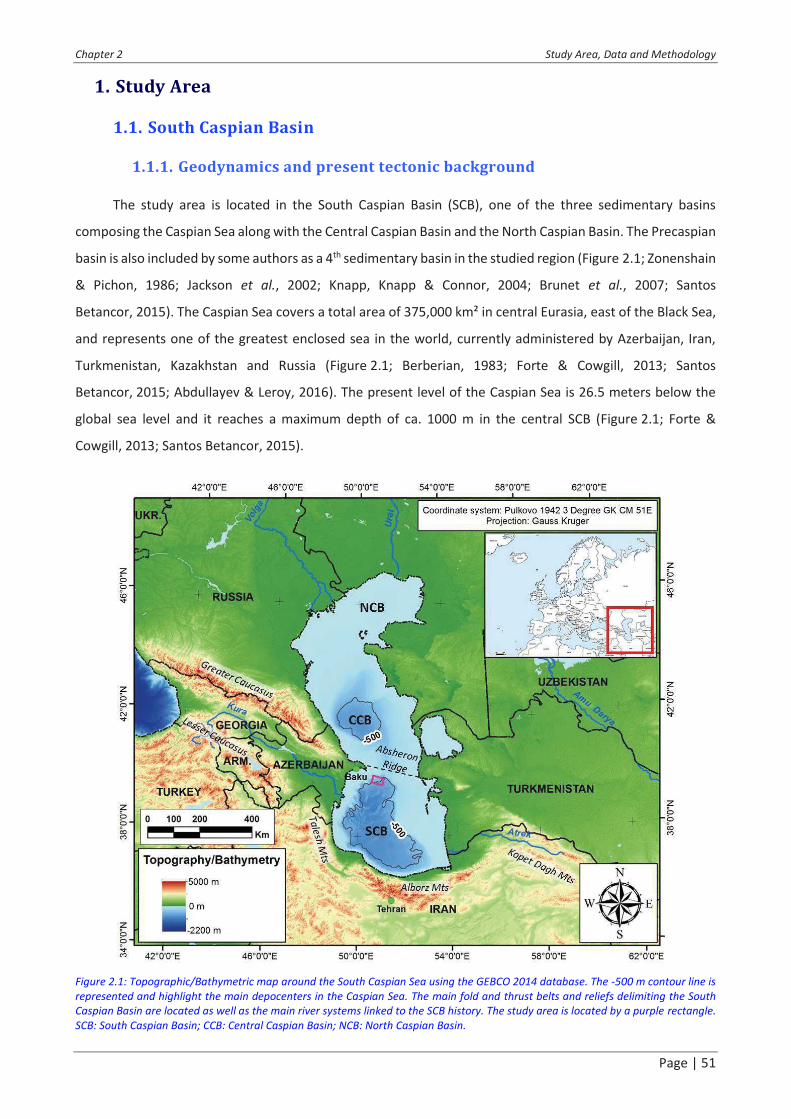
Chapter 2 Study Area, Data and Methodology
Page | 51
1. Study Area
1.1. South Caspian Basin
1.1.1. Geodynamics and present tectonic background
The study area is located in the South Caspian Basin (SCB), one of the three sedimentary basins
composing the Caspian Sea along with the Central Caspian Basin and the North Caspian Basin. The Precaspian
basin is also included by some authors as a 4th sedimentary basin in the studied region (Figure 2.1; Zonenshain
& Pichon, 1986; Jackson et al., 2002; Knapp, Knapp & Connor, 2004; Brunet et al., 2007; Santos
Betancor, 2015). The Caspian Sea covers a total area of 375,000 km² in central Eurasia, east of the Black Sea,
and represents one of the greatest enclosed sea in the world, currently administered by Azerbaijan, Iran,
Turkmenistan, Kazakhstan and Russia (Figure 2.1; Berberian, 1983; Forte & Cowgill, 2013; Santos
Betancor, 2015; Abdullayev & Leroy, 2016). The present level of the Caspian Sea is 26.5 meters below the
global sea level and it reaches a maximum depth of ca. 1000 m in the central SCB (Figure 2.1; Forte &
Cowgill, 2013; Santos Betancor, 2015).
Figure 2.1: Topographic/Bathymetric map around the South Caspian Sea using the GEBCO 2014 database. The -500 m contour line is
represented and highlight the main depocenters in the Caspian Sea. The main fold and thrust belts and reliefs delimiting the South
Caspian Basin are located as well as the main river systems linked to the SCB history. The study area is located by a purple rectangle.
SCB: South Caspian Basin; CCB: Central Caspian Basin; NCB: North Caspian Basin.
Chapter 2 Study Area, Data and Methodology
Page | 52
The origins of the South Caspian Basin trace back to a period spawning between Triassic and Eocene
(Berberian, 1983; Popov et al., 2004; Golonka, 2007; Bochud, 2011). Between Late Triassic and Early Jurassic,
the accretion and collision of several microplates (South Caspian Block, Lut Plate, Central Iran Block, Caucasus
Plate and Alborz Block) along the Eurasian margin, promoted the closing of the Tethys Ocean and the birth
of the Paratethys (Berberian, 1983; Popov et al., 2004; Golonka, 2007; Bochud, 2011). From Jurassic to
Cretaceous, a north-dipping subduction developed along the new continental margin formed by suturing of
the continental blocks (Golonka, 2007; Bochud, 2011). It resulted into a rifting phase due to trench-pulling
effect of the subduction, therefore leading to the opening of a back-arc basin accompanied by active
volcanism, the Greater Caucasus Basin (Berberian, 1983; Zonenshain & Pichon, 1986; Brunet et al., 2007;
Golonka, 2007; Bochud, 2011). This caused thinning of the continental crust and eventually formation of
oceanic crust (Berberian, 1983; Brunet et al., 2007; Golonka, 2007; Bochud, 2011). The Greater Caucasus
Basin reached its maximum extent (900 km wide and 3,000 km long) during the closing of the Paratethys, in
the Late Cretaceous and Early Paleogene (Zonenshain & Pichon, 1986; Golonka, 2007). During the Eocene,
the Lesser Caucasus, Sanandaj Sirjan and Makran blocks were accreted to the Eurasian block, causing the
subduction to jump further north (Golonka, 2007; Bochud, 2011). Since the Oligocene, the Arabian-Eurasian
collision has been separating this basin into smaller ones including the South Caspian depression and the
Black Sea (Zonenshain & Pichon, 1986; Popov et al., 2004; Bochud, 2011), while the South Caspian
microcontinent has been moving northward through rifting between South Caspian and the Alborz Block,
opening the SCB from its SW (Golonka, 2007). The India-Eurasia collision caused deformation of Central Asia,
accommodated through long NW-SE right-lateral transform faults (Golonka, 2007). During the Middle
Miocene, the South Caspian depression separated the deeper eastern part, called the South Caspian Basin,
from the western part, rapidly filled called Kura Basin (Dupuis, 2017). This is due to subsidence of the SCB
through cooling of its oceanic crust and overthrusting on its borders (Berberian, 1983; Zonenshain &
Pichon, 1986; Nadirov et al., 1997), and to the presence of a fold and thrust belt in the Kura Basin that has
been accommodating most of the Arabia-Eurasia collision since the Early Pliocene (Forte et al., 2010).
Subduction of the SCB oceanic crust below the Eurasian plate along the Absheron Ridge was also initiated
during the Miocene (Figure 2.2; Allen et al., 2002; Golonka, 2007; Hollingsworth et al., 2008).
Two elements of the geodynamic history of the basin are still highly discussed. The basement of the
SCB is abnormally thick (8-10 km) for an oceanic crust, but recorded P-wave velocities are about 6.6-7 km/s,
corresponding to an oceanic crust signature (Knapp, Knapp & Connor, 2004; Brunet et al., 2007; Egan et
al., 2009). Therefore, many authors refer to the SCB basement as a �modified� oceanic crust or sub-oceanic
crust (Berberian, 1983; Knapp et al., 2004; Brunet et al., 2007). Nevertheless, some studies proposed another
origin for the basement, arguing that the increasing subsidence of the SCB through its history is inconsistent
with the normal subsidence behavior of an oceanic crust (Artyushkov, 2007). Artyushkov (2007) proposed
the possibility of a deep phase change of gabbro to denser eclogite, process used by Brunet et al. (2007) to
model the subsidence history of the NCB. The age of the initiation of the subduction of the SCB beneath

Chapter 2 Study Area, Data and Methodology
Page | 53
Eurasia is also a matter of debate. Allen et al. (2002) and Khain et al. (2007) calculate, from backstripping of
sedimentary columns and structural analysis of the Absheron ridge, a subduction initiation at the end of
Miocene (5.5 Ma) while Golonka (2007) and Hollingsworth et al. (2008) propose an older origin, spawning
from Early to Middle Miocene (15-10 Ma). All the studies mentioned above agree in defining the SCB as a
remnant of a marginal sea (Berberian, 1983; Zonenshain & Pichon, 1986; Brunet et al., 2007; Golonka, 2007).
Figure 2.2: Simplified tectonic map of the South Caspian area showing the main tectonic units (modified from Brunet et al., 2003). A:
Aghdarband; Ap: Absheron;A Trialet: Achara-Trialet; EO: Erevan-Ordubad; E Pontides: Eastern Pontides; GB: Great Balkhan; Go:
Gorgan; K: Karabakh; L Caucasus: Lesser Caucasus; Na: Nayband; R: Rasht; SP; Scythian platform; TC: Terek � Caspian basin;
WT: Western Turkmenia. The present SCB is delimited by the red dotted line and is located partly onshore.
The South Caspian Basin is at present delimited to the north by the Absheron Peninsula (Baku) and the
Absheron Ridge, to the south by the Alborz massif, to the west by the Greater and Lesser Caucasus and the
Talesh Mountains, and to the east by the Kopet Dagh (Figure 2.1 and Figure 2.2; Berberian, 1983; Priestley et
al., 1994; Allen et al., 2002; Jackson et al., 2002; Vernant et al., 2004; Engdahl et al., 2006; Golonka, 2007).
The Absheron Ridge and Peninsula separate the Central Caspian Basin from the SCB (Khain et al., 2007). The
SCB area is an active tectonic province, currently accommodating the convergence between the Arabian and
Eurasian plates (Figure 2.2; Priestley et al., 1994; Jackson et al., 2002; Guliev & Panahi, 2004; Vernant et al.,
2004; Engdahl et al., 2006; Hollingsworth et al., 2008; Forte et al., 2010).

Chapter 2 Study Area, Data and Methodology
Page | 54
Global Positioning System (GPS) measurements, distribution of earthquakes around the basin as well
as motion on active fault systems allow understanding the present dynamics of the SCB (Figure 2.3; Priestley
et al., 1994; Jackson et al., 2002; Guliev & Panahi, 2004; Vernant et al., 2004; Engdahl et al., 2006;
Hollingsworth et al., 2008; Forte et al., 2010). Overall, the SCB has a motion to the north relative to Eurasia
of 8-10 mm/yr, while the Iran plate has a northward motion relative to SCB of 13-17 mm/yr (Figure 2.3a;
Reilinger et al., 1997; Jackson et al., 2002; Vernant et al., 2004; Santos Betancor, 2015). In detail, there is
differential motion between the east and the west of the basin, which is accommodated by a series of left-
lateral and right-lateral fault systems across the Alborz, Lesser Caucasus and Kopet Dagh mountains (Reilinger
et al., 1997; Jackson et al., 2002; Vernant et al., 2004; Santos Betancor, 2015). Indeed, Forte et al. (2010) and
Reilinger et al. (1997) show that the Kura fold and thrust belt (located along the Kura River Basin, see
Figure 2.1) and the Greater Caucasus, have been accommodating 30 - 50 % of the total convergence between
the Arabian and Eurasian plates since the Early Pliocene. Earthquake distribution and focal mechanisms
around the SCB also evidence that the basin area is tectonically active (Figure 2.3b; Priestley et al., 1994;
Jackson et al., 2002; Engdahl et al., 2006).
Earthquakes mainly concentrate along the basin borders, while the SCB itself shows little tectonic
activity, showing that it behaves as a stable block (Figure 2.3b; Berberian, 1983; Priestley et al., 1994; Jackson
et al., 2002). Different focal mechanisms are detected around the SCB, not deeper than 30 km (Figure 2.3b;
Jackson et al., 2002). Near the basin edges to the south, west and east, focal mechanisms are mainly related
to thrusting, showing the crustal shortening through overthrusting of the various continental blocks over the
SCB (Figure 2.2 and Figure 2.3b; Priestley et al., 1994; Engdahl et al., 2006). The oblique shortening between
Iran and SCB is partitioned between pure thrust and pure strike-slip at high elevation (Priestley et al., 1994;
Jackson et al., 2002; Engdahl et al., 2006). Along the Absheron ridge, earthquake foci are all comprised in a
200 km wide band, at depths varying between 30 and 80 km, showing thrust-related focal mechanisms
(Figure 2.3b ; Priestley et al., 1994; Jackson et al., 2002; Knapp, Knapp & Connor, 2004; Engdahl et al., 2006).
This, along with the downward bending of the crust seismic horizons from south to north are interpreted as
evidence for the northward subduction of the SCB below Eurasia along the Absheron ridge (Priestley et al.,
1994; Jackson et al., 2002; Knapp et al., 2004; Engdahl et al., 2006). The low seismic activity recorded within
the SCB itself (Priestley et al., 1994; Jackson et al., 2002) is explained by the presence of a thick sedimentary
cover sliding over an overpressured detachment level forming high-amplitude folds, and by the presence of
numerous mud volcanoes releasing tectonic stress through another process (Jackson et al., 2002; Guliev &
Panahi, 2004).

Chapter 2 Study Area, Data and Methodology
Page | 55
Figure 2.3: a: Simplified structural map of the Caspian area including GPS-derived estimations for plate velocities. ALBZ: Alborz block;
AN; Anatolian Plate; CAUC: Caucasus Plate; SCB: SCB Block (modified from Santos Betancor, 2015). b: Map showing earthquakes of
the CCB and SCB regions taken from the IRIS catalogue for the period between 1970 and 2010 and classified by depth of their
hypocenters (modified from Santos Betancor, 2015). Blue dotted line marks the oceanic crust of the SCB and the purple rectangles
show the approximate location of the study area.

Chapter 2 Study Area, Data and Methodology
Page | 56
Overall, this shortening resulted in an overall uplift of the the surrounding massifs and triggered strong
subsidence of the SCB creating space for the thick sedimentary succession that fills the basin
(Berberian, 1983; Nadirov et al., 1997; Brunet et al., 2003, 2007; Egan et al., 2009; Guliyev et al., 2011). The
subduction created between 2.4 and 6 km of tectonic subsidence in the last 5.5 My which is faster than
subsidence recorded in typical foreland basins; this subsidence accommodated the rapid sedimentation
recorded in the basin during Pliocene and Quaternary times (Allen et al., 2002; Brunet et al., 2003, 2007;
Egan et al., 2009). The intense shortening resulting from SCB northward subduction generated high-
amplitude folds, detached over a ductile and overpressured interval (Allen et al., 2002; Jackson et al., 2002;
Brunet et al., 2003; Egan et al., 2009).
1.1.2. Paleogeography and regional stratigraphy
The intense and complex tectonic history of the SCB created the conditions to deposit one of the
thickest sediment accumulation in the world (Allen et al., 2002; Morton et al., 2003; Knapp et al., 2004; Smith-
Rouch, 2006; Artyushkov, 2007; Brunet et al., 2007; Guliyev et al., 2011). Very high sedimentation rates are
recorded in the SCB (up to 4.5 km/My), particularly since the Late Miocene, since which nearly 10 km of
sediments were deposited subsequently to a rapid fall in the Caspian Sea level (Tagiyev et al., 1997; Allen et
al., 2002; Inan et al., 2002; Morton et al., 2003; Smith-Rouch, 2006; Brunet et al., 2007; Egan et al., 2009;
Green et al., 2009).
Hereafter, the main regional Mesozoic and Cenozoic stratigraphic units are described in terms of
lithology and deposition environment and the lithostratigraphic column synthetizing the main characteristics
of each stratigraphic unit is given in Figure 2.4.
Jurassic deposits in the SCB area are widespread in the Greater Caucasus (location in Figure 2.1) where
they can reach thicknesses greater than 7000 m (Bochud, 2011; Alizadeh et al., 2017). The sediments were
deposited in a back-arc basin environment and mainly consists of deep marine and slope deposits for the
Lower and Middle Jurassic and consequently to a regression during the Upper Jurassic, deposits change to
shallow marine and slope deposits (Figure 2.4; Golonka, 2007; Bochud, 2011; Alizadeh et al., 2017). Some
volcanic and volcano-clastic intervals are also observed in some areas, as well as black shale formations with
high organic content (Figure 2.4; Green et al., 2009; Bochud, 2011; Alizadeh et al., 2017).
The thickness of Cretaceous sediments locally exceeds 5000 m in the Greater Caucasus and no
depositional hiatus is observed (Bochud, 2011; Alizadeh et al., 2017). They were deposited concordant to
Upper Jurassic interval (Figure 2.4; Golonka, 2007; Bochud, 2011). Rapid transitions from siliciclastic turbidite
facies to carbonate shelf facies are observed in the cretaceous succession of the Greater Caucasus
(Bochud, 2011). Upper Cretaceous deposits are very rich in fossil marine fauna (ammonites, foraminifera,
ostracodes) due to the connection to the Paratethys open sea environment (Golonka, 2007; Bochud, 2011).
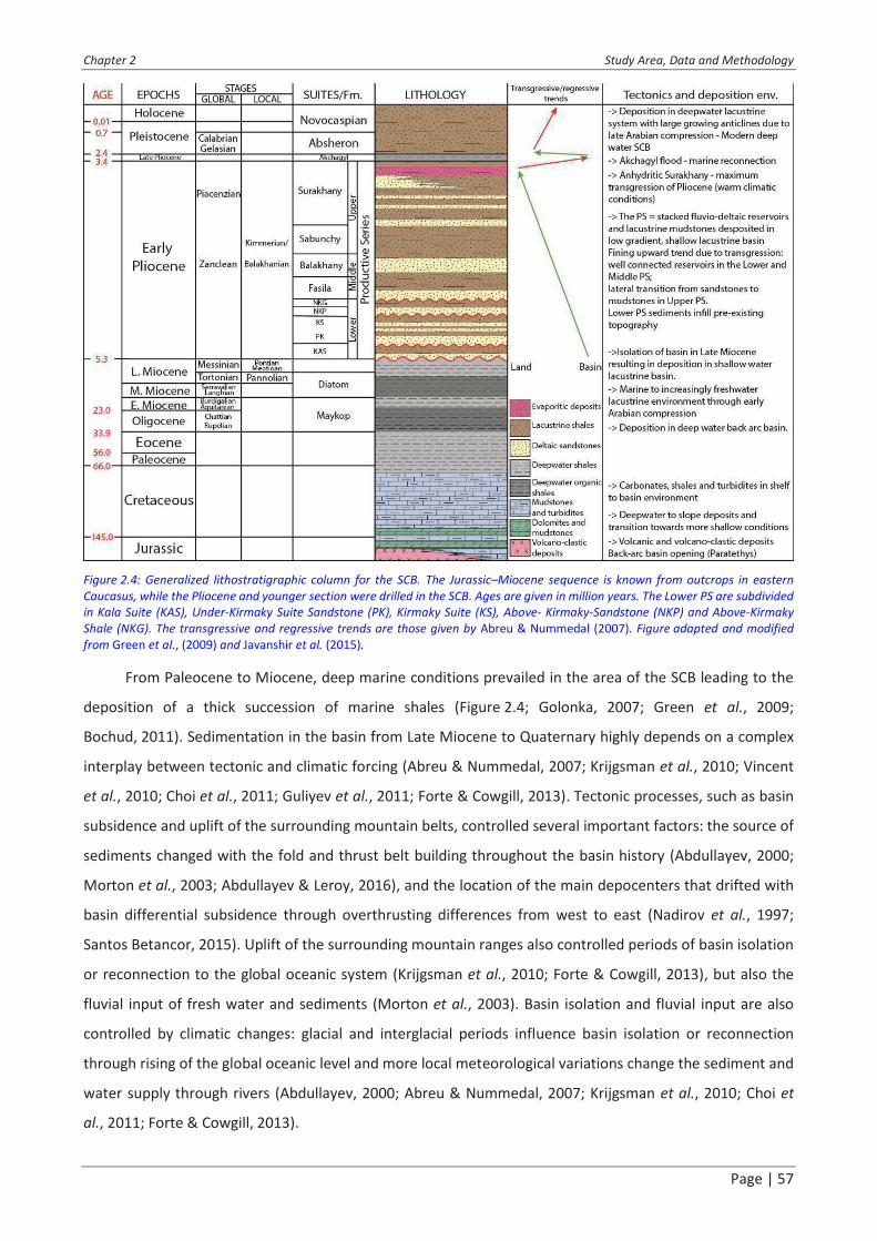
Chapter 2 Study Area, Data and Methodology
Page | 57
Figure 2.4: Generalized lithostratigraphic column for the SCB. The Jurassic�Miocene sequence is known from outcrops in eastern
Caucasus, while the Pliocene and younger section were drilled in the SCB. Ages are given in million years. The Lower PS are subdivided
in Kala Suite (KAS), Under-Kirmaky Suite Sandstone (PK), Kirmaky Suite (KS), Above- Kirmaky-Sandstone (NKP) and Above-Kirmaky
Shale (NKG). The transgressive and regressive trends are those given by Abreu & Nummedal (2007). Figure adapted and modified
from Green et al., (2009) and Javanshir et al. (2015).
From Paleocene to Miocene, deep marine conditions prevailed in the area of the SCB leading to the
deposition of a thick succession of marine shales (Figure 2.4; Golonka, 2007; Green et al., 2009;
Bochud, 2011). Sedimentation in the basin from Late Miocene to Quaternary highly depends on a complex
interplay between tectonic and climatic forcing (Abreu & Nummedal, 2007; Krijgsman et al., 2010; Vincent
et al., 2010; Choi et al., 2011; Guliyev et al., 2011; Forte & Cowgill, 2013). Tectonic processes, such as basin
subsidence and uplift of the surrounding mountain belts, controlled several important factors: the source of
sediments changed with the fold and thrust belt building throughout the basin history (Abdullayev, 2000;
Morton et al., 2003; Abdullayev & Leroy, 2016), and the location of the main depocenters that drifted with
basin differential subsidence through overthrusting differences from west to east (Nadirov et al., 1997;
Santos Betancor, 2015). Uplift of the surrounding mountain ranges also controlled periods of basin isolation
or reconnection to the global oceanic system (Krijgsman et al., 2010; Forte & Cowgill, 2013), but also the
fluvial input of fresh water and sediments (Morton et al., 2003). Basin isolation and fluvial input are also
controlled by climatic changes: glacial and interglacial periods influence basin isolation or reconnection
through rising of the global oceanic level and more local meteorological variations change the sediment and
water supply through rivers (Abdullayev, 2000; Abreu & Nummedal, 2007; Krijgsman et al., 2010; Choi et
al., 2011; Forte & Cowgill, 2013).

Chapter 2 Study Area, Data and Methodology
Page | 58
Isolation and reconnection periods and the input of water through rivers generated high-amplitude
sea-level variations that in turn controlled the basin stratigraphy and sedimentation style (Abdullayev, 2000;
Abreu & Nummedal, 2007; Vincent et al., 2010; Choi et al., 2011; Guliyev et al., 2011; Forte & Cowgill, 2013).
Three main river systems have been supplying sediments to the SCB since the Late Miocene through their
paleo-deltas: the Paleo-Kura delta from the west, the Paleo-Volga from the north, and the Paleo-Amu Darya
from the east (Figure 2.5; Kroonenberg et al., 2005; Smith-Rouch, 2006; Abreu & Nummedal, 2007;
Abdullayev & Leroy, 2016). Depending on the location in the basin, the dominant influence evolve from one
to another of the three deltas (Abdullayev, 2000; Abreu & Nummedal, 2007; Vincent et al., 2010; Guliyev et
al., 2011; Abdullayev & Leroy, 2016).
Figure 2.5: schematic map of the Paleo-drainage systems during the deposition of the Productive Series (Late Miocene-Pliocene). The
possible sources of sediments are displayed as well as the location of the paleo-deltas. The purple box shows the approximate location
of the study area (modified from Smith-Rouch, 2006).
The Maykop Formation, is known as being the main source rock of the Caspian and Black Seas area
(Inan et al., 2002; Smith-Rouch, 2006; Hudson et al., 2008; Guliyev et al., 2011) as well as the decollement
levels for the high amplitude folds of the South Caspian Basin (Allen et al., 2002; Smith-Rouch, 2006; Green
et al., 2009; Santos Betancor, 2015). It was deposited from the Oligocene to the Early Miocene (Figure 2.4;
Hudson et al., 2008; Green et al., 2009; Guliyev et al., 2011; Javanshir et al., 2015) uncomformably over
Mesozoic successions (Knapp, Knapp & Connor, 2004; Javanshir et al., 2015), in a anoxic to suboxic shallow
marine environment, when the Parathetys Sea restriction increased and the basin was bordered by
topographic highs (Inan et al., 2002; Golonka, 2007; Hudson et al., 2008; Bochud, 2011). The sediments
composing this formation are mainly organic-rich and slightly calcareous marine shales with occasional thin
interbeds of coarser detrital material brought by the paleo-Volga river from the north (Figure 2.4; Inan et
al., 2002; Hudson et al., 2008; Green et al., 2009). The organic matter contained in the Maykop formation is
Chapter 2 Study Area, Data and Methodology
Page | 59
mainly from marine sources with a low to moderate input of terrestrial organic matter (Inan et al., 2002;
Smith-Rouch, 2006; Guliyev et al., 2011). Its thickness varies from north to south, ranging from 200 to 1200
m onshore and from 3000 to 1000 m offshore and is buried below a mean 8 km of more recent sediments in
the deepest areas of the basin (Hudson et al., 2008; Green et al., 2009; Bochud, 2011). The Maykop Formation
crops out onshore in the Kura sub-basin, but was never drilled offshore (Hudson et al., 2008; Green et
al., 2009; Bochud, 2011).
The Middle and Late Miocene sediments were deposited in a context of global regression until the
basin isolation after a rapid transgression during early Meotian (local equivalent of the Messinian),
reconnecting the Paratethys and the Mediterranean Sea (Smith-Rouch, 2006; Krijgsman et al., 2010; Forte &
Cowgill, 2013). These sediments are thick clays and diatomic shales deposited in a shallow marine and
lacustrine environment, and comprise another organic rich interval, the Diatom Formation (Figure 2.4;
Hudson et al., 2008; Bochud, 2011; Guliyev et al., 2011; Javanshir et al., 2015; Santos Betancor, 2015). Some
evaporite deposits are found in the Pontian, which is the regional equivalent for the Messinian (Krijgsman et
al., 2010; Forte & Cowgill, 2013; Santos Betancor, 2015).
The Pliocene was dominated by deltaic and lacustrine environment during a regression phase
(Figure 2.4), with sediment input coming from all the topographic highs surrounding the basin through the
three main paleo-rivers (Figure 2.5; Morton et al., 2003; Abreu & Nummedal, 2007; Vincent et al., 2010; Choi
et al., 2011; Forte & Cowgill, 2013; Abdullayev & Leroy, 2016). These deposits, known as the Productive Series
(PS) Formation, are mainly composed of an alternation of connected or isolated sandstone to siltstone bodies
and continuous mudstone intervals (Hinds et al., 2004; Vincent et al., 2010; Choi et al., 2011). The PS
Formation is discordant over the Middle Miocene interval (Knapp et al., 2004; Abreu & Nummedal, 2007).
The sedimentation rate was at its highest magnitude, reaching occasionally 4.5 km/My, with up to 6 km of
PS that were deposited (Tagiyev et al., 1997; Smith-Rouch, 2006; Brunet et al., 2007; Egan et al., 2009; Green
et al., 2009). The subduction-related subsidence of the end of Miocene created enough space to
accommodate such a thickness of deltaic deposits (Allen et al., 2002).
Their lithology strongly varies depending on the location regarding the three main paleo-deltas (
Figure 2.5; Morton et al., 2003; Vincent et al., 2010). The Fig. 8 in Green et al. (2009) shows the stratigraphy
of the PS. It illustrates the complex geometry arising from the paleo-deltas input and their variation with
space and time. However, in the SCB area the Lower PS mainly consist of channelized and sheet flood fluvial
deposits alternating with lacustrine mudstones, and the Upper PS consists of amalgamated braided fluvial
sandstones alternating with alluvial plain and lacustrine deposits (Hinds et al., 2004; Abreu &
Nummedal, 2007). The stratal succession correspond to high-frequencies climatic cycles, sandstone facies
being deposited during lowstand periods and mudstone facies corresponding to transgression and highstand
deposits (Abreu & Nummedal, 2007). The sandstone facies is more continuous in the Lower PS and in the
Kura Basin forming hydraulic connection throughout the SCB, while the Upper PS sandstones are less

Chapter 2 Study Area, Data and Methodology
Page | 60
connected displaying an overall fining-up trend (Figure 2.4; Hinds et al., 2004; Javanshir et al., 2015). At the
top of the Surakhany Formation, the final stage of PS deposition, the regression is maximal and evaporitic
beds are deposited in the northern part of the basin (Javanshir et al., 2015; Dupuis, 2017). Farther south, an
erosional event is recorded without evaporitic deposition (Santos Betancor, 2015). This interval will be called
Anhydritic Surakhany hereafter.
The Akchagyl Formation was deposited on a period extending over 700,000 years during the Late
Pliocene (2.4-3.4 My) and was not deposited synchronously over the whole basin (Forte et al., 2015). It was
deposited during a major regional transgression, after a marine flooding event through a reconnection of the
Caspian Sea with the Black Sea and potentially with the Mediterranean (Green et al., 2009; Bochud, 2011;
Forte & Cowgill, 2013). In several location of the Kura Basin, the Akchagyl Formation lies unconformably over
older Miocene intervals due to this regional transgression (Bochud, 2011). The Akchagyl Formation is a
condensed interval and its composition varies between shallow marine and fresh water facies (western part
of Kura Basin), and deep water clayey facies interlayered with mud-rich turbidites in the SCB (Figure 2.4;
Abdullayev, 2000; Green et al., 2009; Bochud, 2011; Santos Betancor, 2015). The mud-rich turbidites were
supplied by the Paleo-Amu Darya (Figure 2.5; Abdullayev, 2000).
The Absheron Formation was deposited from the Early Pleistocene (2.4 Ma) to present during a
transgression and the subsequent regression (Green et al., 2009; Forte & Cowgill, 2013; Santos
Betancor, 2015). The Absheron deposits consist of prograding and deepwater fan systems and slumps
(Abdullayev, 2000; Green et al., 2009). Their lithology varies from clays to sandstones with some shell-rich
limestone occurrences, volcanic ashes and conglomerates (Figure 2.4; Bochud, 2011; Santos Betancor, 2015).
The depositional environment that prevailed was similar to the present situation: deep-water lake with
brackish conditions (Abdullayev, 2000; Green et al., 2009; Forte & Cowgill, 2013; Santos Betancor, 2015). The
Novocaspian Formation is differentiated from the Absheron Suite on several studies (Abdullayev, 2000;
Imbert et al., 2014). This formation corresponds to deposits younger than 0.7 Ma and are mainly deep
lacustrine shales (Figure 2.4; Green et al., 2009; Imbert, Geiss & Fatjó de Martín, 2014).
1.1.3. Oil & gas potential and mud volcanism
The South Caspian Basin is one of the most prolific hydrocarbon (HC) provinces in the world and has
been exploited for more than 150 years (Smith-Rouch, 2006; Abreu & Nummedal, 2007; Alizadeh et
al., 2017). Areas like the Absheron Peninsula, Absheron Ridge, the Kura basin and the Shelf margin of
Azerbaijan have been intensively explored and produced (620 oil and gas fields discovered) while the deep
water SCB and Turkmenistan shelf are areas less understood and remain frontier exploration areas (Smith-
Rouch, 2006; Abreu & Nummedal, 2007; Alizadeh et al., 2017).
The first favorable factor for the presence of such HC accumulations in the SCB region is the presence
of several mature source rocks (Tagiyev et al., 1997; Inan et al., 2002; Smith-Rouch, 2006; Guliyev et
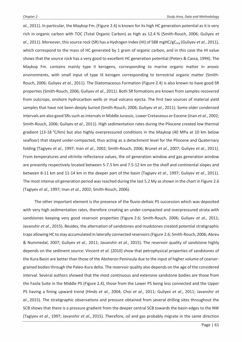
Chapter 2 Study Area, Data and Methodology
Page | 61
al., 2011). In particular, the Maykop Fm. (Figure 2.4) is known for its high HC generation potential as it is very
rich in organic carbon with TOC (Total Organic Carbon) as high as 12.4 % (Smith-Rouch, 2006; Guliyev et
al., 2011). Moreover, this source rock (SR) has a Hydrogen Index (HI) of 588 mgHC/gCorg (Guliyev et al., 2011),
which correspond to the mass of HC generated by 1 gram of organic carbon, and in this case the HI value
shows that the source rock has a very good to excellent HC generation potential (Peters & Cassa, 1994). The
Maykop Fm. contains mainly type II kerogens, corresponding to marine organic matter in anoxic
environments, with small input of type III kerogen corresponding to terrestrial organic matter (Smith-
Rouch, 2006; Guliyev et al., 2011). The Diatomaceous Formation (Figure 2.4) is also known to have good SR
properties (Smith-Rouch, 2006; Guliyev et al., 2011). Both SR formations are known from samples recovered
from outcrops, onshore hydrocarbon wells or mud volcano ejecta. The first two sources of material yield
samples that have not been deeply buried (Smith-Rouch, 2006; Guliyev et al., 2011). Some older condensed
intervals are also good SRs such as intervals in Middle Jurassic, Lower Cretaceous or Eocene (Inan et al., 2002;
Smith-Rouch, 2006; Guliyev et al., 2011). High sedimentation rates during the Pliocene created low thermal
gradient (13-18 °C/km) but also highly overpressured conditions in the Maykop (40 MPa at 10 km below
seafloor) that stayed under-compacted, thus acting as a detachment level for the Pliocene and Quaternary
folding (Tagiyev et al., 1997; Inan et al., 2002; Smith-Rouch, 2006; Brunet et al., 2007; Guliyev et al., 2011).
From temperatures and vitrinite reflectance values, the oil generation window and gas generation window
are presently respectively located between 5-7.5 km and 7.5-12 km on the shelf and continental slopes and
between 8-11 km and 11-14 km in the deeper part of the basin (Tagiyev et al., 1997; Guliyev et al., 2011).
The most intense oil generation period was reached during the last 5.2 My as shown in the chart in Figure 2.6
(Tagiyev et al., 1997; Inan et al., 2002; Smith-Rouch, 2006).
The other important element is the presence of the fluvio-deltaic PS succession which was deposited
with very high sedimentation rates, therefore creating an under-compacted and overpressured strata with
sandstones keeping very good reservoir properties (Figure 2.6; Smith-Rouch, 2006; Guliyev et al., 2011;
Javanshir et al., 2015). Besides, the alternation of sandstones and mudstones created potential stratigraphic
traps allowing HC to stay accumulated in laterally connected reservoirs (Figure 2.6; Smith-Rouch, 2006; Abreu
& Nummedal, 2007; Guliyev et al., 2011; Javanshir et al., 2015). The reservoir quality of sandstone highly
depends on the sediment source: Vincent et al. (2010) show that petrophysical properties of sandstones of
the Kura Basin are better than those of the Absheron Peninsula due to the input of higher volume of coarser-
grained bodies through the Paleo-Kura delta. The reservoir quality also depends on the age of the considered
interval. Several authors showed that the most continuous and extensive sandstone bodies are those from
the Fasila Suite in the Middle PS (Figure 2.4), those from the Lower PS being less connected and the Upper
PS having a fining upward trend (Hinds et al., 2004; Choi et al., 2011; Guliyev et al., 2011; Javanshir et
al., 2015). The stratigraphic observations and pressure obtained from several drilling sites throughout the
SCB shows that there is a pressure gradient from the deeper central SCB towards the basin edges to the NW
(Tagiyev et al., 1997; Javanshir et al., 2015). Therefore, oil and gas probably migrate in the same direction

Chapter 2 Study Area, Data and Methodology
Page | 62
(Tagiyev et al., 1997; Guliyev et al., 2011), but their migration is most of all impacted by tectonic structures
such as folds and faults that trap HC (Imbert, pers. comm., 04-06-2019). Grosjean et al. (2009) and Javanshir
et al. (2015) show that hydrodynamism results in tilting of the HC-water contacts, thereby shifting HC
accumulations towards the N flanks of anticlines.
Figure 2.6: HC generation and accumulation temporal chart for the Oligocene�Miocene Maykop/Diatom Total Petroleum System in
the South Caspian Basin Province. Ak-Ap: Akchagyl and Absheron intervals. The critical moment correspond at the time when all the
criteria for oil & gas generation, accumulation and preservation were present and correspond to the Akchagyl strata deposition (from
Smith-Rouch, 2006).
The deposition of thick deep water marine mudstones during the Quaternary period allowed the whole
Oligocene-Pliocene interval to be deeply buried and trapped below an efficient thick seal (Figure 2.6;
Abdullayev, 2000; Smith-Rouch, 2006; Green et al., 2009; Bochud, 2011).
The intense compression caused by Arabic Plate convergence towards Eurasia coupled with the
presence of a good detachment level allowed the creation of high-amplitude folds in all the SCB and Kura
Basin from Pliocene to present (Allen et al., 2002; Knapp et al., 2004; Smith-Rouch, 2006; Forte et al., 2010).
They form topographic highs in reservoirs, creating excellent structural traps for HC (Figure 2.6; Smith-
Rouch, 2006; Guliyev et al., 2011; Javanshir et al., 2015). Many anticlines are cored by deeply rooted thrusts
and overpressured mobile Maykop creating potential vertical pathways for HC fluids (Smith-Rouch, 2006;
Guliyev et al., 2011; Santos Betancor & Soto, 2015).
The SCB is also known for the presence of numerous MVs onshore and offshore (Milkov, 2000;
Dimitrov, 2002; Kopf, 2002; Yusifov & Rabinowitz, 2004). Most of the studied MVs are interpreted as being
sourced from the Maykop from geochemical and biostratigraphic analysis of clasts onshore and from
geometric considerations offshore (Dimitrov, 2002; Kopf, 2002; Yusifov & Rabinowitz, 2004; Stewart &
Davies, 2006). However, some authors argue that other sources may be possible, in particular for recent or
active structures where the Maykop is deeply buried (Yusifov & Rabinowitz, 2004; Dupuis, 2017; Blouin et
al., 2019). One general observation is that all the observed MVs are aligned along or near the anticline crests

Chapter 2 Study Area, Data and Methodology
Page | 63
(Fowler et al., 2000; Yusifov & Rabinowitz, 2004; Stewart & Davies, 2006; Roberts et al., 2010; Dupuis, 2017;
Blouin et al., 2019). Fowler et al. (2000) and Yusifov & Rabinowitz (2004) correlated the MV formation to the
growing of folds, the timing of HC generation and accumulation and to high sedimentation rates during
Pliocene.
1.2. Absheron fold: gas-condensate field and geohazards
Total has been operator of the Absheron gas condensate field (see location in Figure 2.1), located 100
km at the SW of Baku, since 2009, with a first major discovery in 2011 (Gautherot et al., 2015). This gas field
could represent reserves of 350 billion cubic metres (Bcm) of gas and 45 million tons of gas condensate and
production may start in 2021 (Wikipedia: Absheron gas field, 2018).
The exploration phase between 1997 and 2006 started with a first well drilled with no HC discovered
and a 650 km² 3D seismic survey acquired (Gautherot et al., 2015; Unterseh & Contet, 2015). A first
estimation of geohazards was conducted based on seismic data, evidencing the active AMV, regional scale
MTCs and a large slope failure scar at seabed (Unterseh & Contet, 2015). Imbert, Geiss and Fatjó de
Martín (2014) studied the presence of a buried, subcircular crater, filled with MTCs interpreted as being
potentially the result of fluidification of sediments due to gas exsolution triggered by unloading of the strata
by a massive slump. The MV was notably assessed in terms shallow geometry and a comparison to onshore
flat MVs by Dupuis (2017). Up to three massive bevel-shaped thrusted mudflows were described from the
seismic data (Dupuis, 2017).
However, the resolution of the seismic data is not sufficient in order to assess with precision the
geohazards over the Absheron field and notably to understand the recent activity of the AMV (Contet &
Unterseh, 2015; Unterseh & Contet, 2015). The high-resolution geophysical and geotechnical data highlights
the shallow complexity and geohazards at the Absheron site, mostly due to the interaction of several factors
such as tectonics, mud volcanism, mass transport deposits and gaseous fluid upward migration (Unterseh &
Contet, 2015). Gas migration generates several geohazards, such as shallow gas and the potential slope
failure it may trigger, the presence of the active MV, seepages through faults and pockmarks (Unterseh &
Contet, 2015). The high-resolution data also allows evidencing five recent mudflows as well as detail on the
surface structure of the AMV with several gryphons and mud pies (Kieckhefer et al., 2003; Contet &
Unterseh, 2015; Dupuis, 2017). Contet & Unterseh (2015) dated these mudflows using palynological and
biostratigraphic analysis of hemipelagites draping the mudflows and concluded that the AMV was active for
the last 5000 years BP. They also evidenced that the last major recorded mudflow dated from 735 years BP,
showing that the last major eruption is older than the mean time recurrence between mudflow (500 years),
concluding that the area surrounding the AMV is not safe for drilling operations as the AMV may erupt in the
near future (Contet & Unterseh, 2015). Dupuis (2017) calculated the volume of these five young events: each
mudflow represent at least 0.5 km3 of mud.

Chapter 2 Study Area, Data and Methodology
Page | 64
MTCs are a major feature in recent stratigraphic intervals (Absheron suite, Figure 2.4), and Imbert,
Geiss & Fatjó de Martín (2014) identified 4 MTCs in this interval. Dupuis (2017) shows that MTCs interact
with the AMV: MTCs abut on the AMV, deform around the volcano and finally deviate from their initial
direction.
2. Data acquisition and location
2.1. 3D seismic survey
Figure 2.7: Seafloor depth map extracted from the 3D seismic survey, showing the location of the other surveys and samples used
during this research. The AMV is visible as a light blue patch where the dataset is denser. Seafloor depth is given in meters below
mean sea level. The Purple rectangle shows the maximum extent of the 3D seismic survey, the black polygon shows the extent of the
multibeam echo sounder survey, and the red rectangle, the area where backscattering image was processed. Samples are represented
with different symbols depending on their type. Red circles with crosses: exploration wells; orange circles with dots: rotary drillings
and CPT measurements; blue pentagons: piston cores from AUV survey, 2014; yellow square: box core from AUV survey, 2014; green
triangles: samples for biostratigraphy from Chevron survey, 1999.
The 3D seismic volume covers 650 km², in water depths ranging from 180 to 700 m (Figure 2.7). The
seismic sections presented in this thesis are from Kirchhoff pre-stack time migration (PSTM) processing and
pre-stack depth migration (PSDM) reprocessing (Robein, 2010), which was applied on 550 km² of the seismic

Chapter 2 Study Area, Data and Methodology
Page | 65
survey. The velocity model used in the reprocessing aimed to improve the imaging of the deep structures
(thrust, dips), taking into account the lateral velocity variations across the thrust as well as the velocity
heterogeneity in the shallow intervals due to the presence of the mud volcano and free gas (F. Adler,
12/12/2018, personal communication). The model parametrization is a vertical transverse isotropy (VTI) that
considers the vertical anisotropy imposed by the sedimentary strata (Robein, 2010). The model was entirely
built by tomographic inversion (Robein, 2010), and in the deep part, it was corrected using an interpretative
method in order to preserve the structural coherency and to fit the well data (F. Adler, 12/12/2018, personal
communication). The seismic volume is composed by 2203 inlines and 2120 crosslines with 12.5 m inline and
18.5 crossline spacing. The vertical resolution varies with depth as it depends on interval velocity. From visual
observations of the sections, we estimate a resolution ca. 20 m in the strata above 2000 m, progressively
decreasing to 150 m at 11 km.
2.2. Geotechnical and geophysical survey
A marine geological and geotechnical survey of the seabed above the Absheron gas discovery was
carried out in 2014 in order to better constrain and delineate geological hazards associated with the mud
volcano (Contet & Unterseh, 2015; Unterseh & Contet, 2015). The different data presented hereafter are
extracted from several confidential Total proprietary reports written and produced by Fugro Survey Limited
Caspian (G. Dan & S. Po, 12/09/2017, personal communication).
2.2.1. Geophysical dataset
An AUV-mounted multibeam echosounder (MBES Kongsberg EM 2040; Horvei & Nilsen, 2010) was
used to acquire a high-resolution map to study the detailed surface morphology of the AMV (Figure 2.7;
Contet & Unterseh, 2015; Unterseh & Contet, 2015). The AUV survey was carried out along 228 NNE-SSW
directed inlines with 175 m of spacing and 88 crosslines oriented WNW-ESE with a spacing ranging from 500
m to 1 km. The AUV navigated at 60 m above seafloor on inlines to guarantee maximum coverage and 40 m
above seafloor on crosslines. The bathymetry is obtained from the two-way travel time of the emitted signal
(Zitter, 2004). The bathymetric map has been processed with a resolution of 3 m by 3m (Contet &
Unterseh, 2015). The backscatter map was also acquired, allowing estimating seafloor roughness and
differentiating mudflow deposits and clasts from the surrounding hemipelagic sediments (Zitter, 2004).
Backscatter map results from the calculation of the energy of the incident signal dispersed at the contact of
irregular surfaces (Zitter, 2004).
In parallel of MBES, a chirp Sub-bottom profiler mounted on the AUV allowed imaging the shallow
succession of sediments over and around the AMV with a vertical resolution of 0.3 m and a penetration of
40 to 50 meters below seafloor (Contet & Unterseh, 2015). The velocity used in order to convert in depth the
different time sections was 1500 m/s, which was measured from in situ on rotary drilling sites.

Chapter 2 Study Area, Data and Methodology
Page | 66
2.2.2. Coring and in situ mechanical measurements
The geotechnical/geological survey from 2014 includes rotary drilling, AUV (Autonomous Underwater
Vehicle) sampling with a box corer and a 6 m long Kullenberg piston corer (Kullenberg, 1947) as well as in situ
geotechnical testing (CPTu, Cone Penetration Testing; Lunne, 2010) in and around the AMV (Figure 2.7). Well
logging and CPT were performed on two boreholes using the Seafloor Drill equipped with a penetration and
coring system (Total proprietary report, G. Dan & S. Po, 12/09/2017, personal communication): CH2 was
located outside the mud volcano area to provide a stratigraphic reference in continuous series, and MVF1
sampled on a mud volcano flow (Figure 2.7).
CPTu is an in situ penetration test procedure consisting in pushing vertically in sediments a steel rode
and allowing measuring the soil resistance (Lunne et al., 1997; Boggess & Robertson, 2011). Integrated
probes allow a continuous recording of penetration depth, cone resistance, sleeve friction and in situ pore
pressure which is measured through a differential pore pressure sensor (Lunne et al., 1997; Boggess &
Robertson, 2011). The well logging consisted notably in measuring the in situ acoustic properties of
sediments (P-wave and S-waves) by emitting signals from a source and receiving them at several (Total
proprietary report, G. Dan & S. Po, 12/09/2017, personal communication). Measurements were either made
during penetration interruption (Seismic CPT) through downhole tests where the penetration rode includes
geophones, either once the penetration tests reached their maximum depth after borehole casing. In the
latter, geophones are placed at given depth for each measurements (Total proprietary report, G. Dan & S.
Po, 12/09/2017, personal communication).
Along with CPT logging, rotary drilling allowed the sampling of 35 meters of sediment, notably coring
through several mudflows (Total proprietary report, G. Dan & S. Po, 12/09/2017, personal communication).
These samples allowed the dating of the drilled recent mudflows using pollen content and radiocarbon (14C)
(Contet & Unterseh, 2015). Another offshore survey was completed in 1999 by Chevron in order to date the
mud emitted at the AMV using biostratigraphic content in the mud breccia clasts and the mud matrix. Several
samples were collected at several locations, notably on the main mudflow (Figure 2.7).
2.3. Exploration wells
During exploration and appraisal stages of the Absheron field, two exploration wells were drilled. The
first one, ABX-1A was drilled by Chevron in 2001 on the southern flank of the Absheron anticline and reached
6529 m TVD/MSL (True Vertical Depth below Mean Sea Level) and no commercially productive HC reservoirs
was discovered. A second exploration well was drilled by Total in 2011 on the northern flank of the Absheron
anticline and reached 6823.5 m TVD/MSL. The well discovered gas in several reservoirs of the Middle and
Lower PS. Locations of both wells are given in Figure 2.7. During drilling, several measurements and analyses
were carried out and two types of logging tools were used: LWD (Logging While Drilling) tools, which are
attached to the drill string and allows logging without stopping drilling operations and WL (Wireline) tools

Chapter 2 Study Area, Data and Methodology
Page | 67
that are brought down in the borehole when the drilling bit is out. We used LWD recordings preferred for
first stratigraphic correlations and wireline logs to get more detailed measurements over specific intervals.
The main source for the principles of log data acquisition and interpretation presented hereafter are
the Crain�s Petrophysical Handbook online (Crain, 2018), which is updated annually.
2.3.1. Gamma-ray and caliper logs
Three radioactive elements (Potassium, K, Thorium, Th, and Uranium, U) are widespread in nature, as
main constituents of some common or accessory minerals (e.g. K in some feldspars and clay minerals derived
from their alteration, or in K-evaporites; Th in monazite), or can be adsorbed like U on organic matter (Howell
& Froscht, 1939; Marett et al., 1976; Crain, 2018). As a result, rocks and sediments, depending on their
mineral content naturally emit a certain amount of gamma radiation (Howell & Froscht, 1939; Marett et
al., 1976; Crain, 2018). Gamma ray (GR) logging tools measure the amount of GRs emitted by the formations
surrounding them in an open or cased borehole, which is commonly correlated to the amount of clay minerals
present among sediments, as they are rich in radioactive potassium and can charge in uranium and thorium
through cationic exchange capacity (Howell & Froscht, 1939; Crain, 2018). Therefore, this tool allows
differentiating between clay-rich lithologies (shales, claystones) and other lithologies (Marett et al., 1976;
Segesman, 1980; Crain, 2018). However, no distinction is possible through this tool between sandstones and
carbonates for instance. The maximum GR value recorded in a formation containing shale is generally
referred to as the shale base line. Any deflection to smaller GR values indicates the presence of non-
radioactive minerals, typically quartz grains or carbonates formation is getting coarser (Abdelaziz, 2016).
The caliper log continuously records the diameter of the borehole, allowing to control its integrity
(Segesman, 1980; Snyder & Fleming, 1985). The tool uses several articulated arms that are kept in contact
with the wall of the drill hole, so it can record any variation of its diameter (Segesman, 1980). As the
resistance of the wall highly depends on the constitutive sediment mechanical properties and cohesion, the
variation of the size and shape of the borehole can be related to lithologies and correlates most of the time
with GR log. For instance, shales have a tendency to swell or to form cavings during drilling operations, while
permeable sandstones may absorb the filtrate of drilling fluids and leave the solid fraction as a �mud cake�
on the borehole wall.
2.3.2. Sonic logs
Sonic tools consist of an acoustic source (with a typical frequency of 10-20 kHz) and at least 2 receivers
mounted 2 feet apart on the logging tool and rely on Snell�s law describing the propagation of acoustic waves
at an interface of two different materials (Segesman, 1980; Crain, 2018). The acoustic velocity in fluid-
saturated rocks is governed by physical properties synthetized in the Biot-Gassmann equations (Biot, 1956;
Crain, 2018). Borehole wall sediments generally have a significantly higher acoustic velocity than the drilling

Chapter 2 Study Area, Data and Methodology
Page | 68
mud, so that the first signal received at the receivers is the signal refracted through the intact formation
(while the direct wave propagating in the mud is received afterwards); the tool typically measures the time
difference between first arrivals at two receivers mounted 2 feet apart, directly providing a slowness in µs/m
(the inverse of the velocity; Crain, 2018). Using at least two receivers allows compensating for the variations
in drilling mud thickness (Segesman, 1980).
Empirical relationships are commonly used to estimate formation density and porosity from acoustic
velocity (Wyllie et al., 1958; Segesman, 1980). In addition, the presence of free gas in formation fluids
decreases acoustic velocity, so that the presence of gas may be detected on sonic logs (Helgerud et al., 1999).
2.3.3. Density log
This sidewall tool emits GR from an artificial radioactive source into an uncased drilled formations
(Segesman, 1980; Snyder & Fleming, 1985). The GR interacts through Compton scattering process
(Compton, 1923) with the electron cloud of the different elements present in the sediments (solids and fluids)
and loses energy (Snyder & Fleming, 1985; Abdelaziz, 2016; Crain, 2018). The detector of the logging tool, a
scintillation counter, measures the intensity of the bask-scattered GR, which is inversely proportional to the
electron density of the formation, itself relating directly to its bulk density (Snyder & Fleming, 1985;
Abdelaziz, 2016; Crain, 2018). The density of the formation depends on its lithology, its porosity and the
density and saturation of the pore fluids (Abdelaziz, 2016). Dense formations will absorb more GR than low-
density formations as they are formed by heavier elements having a denser electronic cloud.
2.3.4. Neutron logs
The neutron logs allows quantifying the porosity of the drilled formations and can be used as a
determining factor for lithology when coupled to a density log (Segesman, 1980; Abdelaziz, 2016;
Crain, 2018). The logging tool is equipped with a neutron source that emits neutron with a high velocity into
the sediments. Neutrons interact with hydrogen atoms contained in the tested formation through elastic
scattering mechanism, slowing down until being captured by atoms (Snyder & Fleming, 1985;
Abdelaziz, 2016; Crain, 2018). Therefore, the richest in hydrogen the formation will be, the faster neutrons
will be slowed down. The neutron porosity measures altogether the drilling mud, the hydrocarbon portion
(present in the pore space), the shale portion and the matrix portion each one of them containing hydrogens
(Abdelaziz, 2016; Crain, 2018). The presence of HC fluids, and in particular methane, will generates a neutron
porosity that is smaller, allowing to detect the presence of gas accumulations when combining the neutron
log with other porosity logs (such as density logs).
2.3.5. Resistivity logs
This method consists in characterizing the sediments surrounding the borehole by measuring its
electrical resistivity, namely the capacity that the material has to oppose the circulation of an electric current

Chapter 2 Study Area, Data and Methodology
Page | 69
(Crain, 2018). In boreholes, rocks and sediments acts as electric insulators, while the fluids they contain acts
as conductors with the exception of HC fluids, which are even more resistive than sediments. Therefore,
resistivity logs are a good tool for detecting HC during drilling operations (Geary, 2018). Classical resistivity
logs have to be acquired in a borehole saturated with conductive mud or water (Geary, 2018). Oil-based
drilling muds are very resistive so that electrical current is not able to circulate and to reach the tested
formation (Doll, 1949; Snyder & Fleming, 1985). Therefore, in wells where oil-based drilling mud is used,
resistivity is measured through induction tools (Doll, 1949; Snyder & Fleming, 1985). The electrical current is
induced into the tested formation based on Maxwell�s equations that gives the foundation of
electromagnetism (Crain, 2018). Thus, the probe does not need to be in direct contact with the borehole wall
(Doll, 1949).
Several source/receiver couples are used to measure resistivity, the distance between each source and
each receiver being designed to measure resistivity at a certain distance from the borehole (Doll, 1949;
Geary, 2018). Resistivity logs are used in the assessment of porosity, water saturation and presence of HC
(Snyder & Fleming, 1985; Crain, 2018). Moreover, if permeability is low, drilling fluids will not be able to
invade the pore space and will stay close to the borehole walls. Thus, resistivity measured in the close field
and far field may be different as fluids allowing current to circulate are different. Conversely, if permeability
is high, drilling fluids will be able to flow into the pore space, implying that close field and far field resistivity
will be identical. Thus, resistivity logs allow to test the permeability of the drilled formations (Crain, 2018;
Geary, 2018).
2.3.6. Lithology
Lithology at both wells is interpreted from the logs, calibrated by the analysis of ditch cuttings, which
are fragments of solid material from the drilled stratigraphic intervals. They are produced from the rocks
broken by the advance of the drilling bit and are moved to the surface along with the drilling mud that
circulates in order to keep the borehole open by sustaining a pressure higher than the formation pressure.
The cuttings are then separated from drilling fluids using shakers or centrifuges. They are sampled by the
wellsite geologist at regular intervals, e.g. every 10 or 20 m in intervals with limited economic interest and
every 5 m in intervals of specific interest. The mud logger or wellsite geologist then studies each interval.
Visual observation and mineral recognition as well as X-ray diffractometric measurements allows defining
the mineral composition and lithology on each studied interval. However, these analysis may be either
polluted by drilling mud components (notably barite when high formation pressure are encountered) or
samples are washed taking the risk to lose the finer fraction composing the interval lithology (clay minerals
notably).
The GR, caliper and resistivity LWD logs along combined with cutting analysis allows reconstructing a
preliminary lithological log describing the sediment succession drilled and presented in the �quick-look� log

Chapter 2 Study Area, Data and Methodology
Page | 70
which is plotted during drilling operations (Figure 2.8a). This log is then detailed, completed and corrected
using the other type of acquired data like the sonic log, and coupled neutron and density plot that allows
highlighting the presence of reservoir facies (yellow areas in the sonic column of Figure 2.8b). Moreover, the
presence of HC can be highlighted by the resistivity signal.
2.3.7. Formation pressure logs, rock strength, temperature and gas out
Two types of formation pressures are provided in the Absheron exploration wells. The shale pressure
is an estimate that results from Eaton�s method applied to the sonic logs (Eaton, 1975). Eaton�s method
consists in comparing the sonic log with a linear trend based on the highest sonic values in completely shaly
intervals and considered as reflecting the �normal compaction trend�. Any negative deviation from this curve
is considered to result from undercompaction due to pore overpressure and is therefore calculated along the
entire borehole like the sonic log. In porous-permeable intervals, pressure in situ reservoir pore pressure was
measured directly using Schlumberger�s StethoScope pressure WL tool (Schlumberger, 2019). Only target
reservoirs were tested, and some measurements failed due to tool issues.
Fracturing pressure log is calculated from shale and reservoir pressures, adjusted by calibration to leak-
off tests or formation integrity tests (Lin et al., 2008), as well as downhole mud losses.
Wireline tools measured temperatures at different points in either open hole or cased hole.
Additional information, such as the occurrence and composition of free gas is available. Free gas are
emitted and recorded at the flow line in the shaker room within the drilling mud and cuttings recovered
during drilling operations. These data gives information on the presence of gas reservoirs along the drilled
stratigraphic column as well as the nature and composition of these gases, and potentially the maturity of
source rocks.

Chapter 2 Study Area, Data and Methodology
Page | 71
Figure 2.8: Log data from well ABX2 presented"as"an"example"of"lithology"interpretation."a:"�quick-look�"log"plotted"during"drilling"operations"for"monitoring"purposes."The"main"data"acquired"with"LWD"
tools are the gamma-ray (GR) signal (green) and the resistivity (shallow in blue, deep in red). These geophysical data are coupled with cuttings analysis in order to present a preliminary lithological
section. b: final composite log, with all geophysical data obtained over a given section (GR; resistivity, shallow and deep field; sonic, DTP for P-waves and DTS for S-waves; density; neutron). Using data
from resistivity coupled with sonic, and superimposed neutron and density, it is possible to refine the lithological log notably by precisely highlighting reservoir facies (yellow color, right column).

Chapter 2 Study Area, Data and Methodology
Page | 72
3. Methods
3.1. Seismic interpretation
Each medium has its own acoustic impedance. Therefore, when a seismic signal reaches a limit
between two media with different impedances, part of the acoustic signal will be reflected (Nely, 1986). A
seismic signal can be decomposed in wavelets which are characterized by their polarity, their amplitude (peak
area), its period and its phase (Nely, 1986). Normal polarity is given by the seafloor polarity, which in the data
presented hereafter is a wavelet with a strong central positive amplitude surrounded by two weak negative
amplitudes. Thus, the normal polarity is a strong positive peak enclosed between two weak negative peaks
indicating a step-wise increase in impedance. The opposite shows a step-wise decrease in impedance
(Nely, 1986; Ricker, 1953).
Seismic interpretation was carried out using the Total in-house software Sismage (Guillon &
Keskes, 2004). From the 3D seismic cube, we calculated the seismic coherency attribute, which can be
projected on horizontal slices or seismic horizons. Seismic coherency allows to differentiate laterally
continuous areas (undisturbed deposits) from low continuity zones (faults or mud volcano deposits for
instance) (Bahorich & Farmer, 1995). Horizons were propagated and named according to stratigraphic limits
encountered in the two exploration wells drilled on the Absheron anticline (Figure 2.7 for location). These
stratigraphic limits are interpreted based on cuttings analysis and gamma-ray, sonic and resistivity logs (see
Chapter 2:2.3). Between two horizons, it is possible to extract layers of regular thickness on which the Root
Mean Square (RMS) of the seismic amplitude can be calculated. This allows visualizing in map view the spatial
distribution of sediment bodies whose impedance contrasts with the background, thus imaging for instance
channels, mudflows, and pipes.
Several imaging artifacts may arise from the recording and processing of seismic data. The presence of
free gas is a well-documented cause of signal attenuation, causing what is known as wipe-out (Graue, 2000;
Benjamin & Huuse, 2017). Several studies showed a strong seismic signal attenuation below active mud
volcnaoes (Graue, 2000; Benjamin & Huuse, 2017). Mud volcanoes are known to be accompanied by large
emissions of free gas (Kopf, 2002; A. Mazzini & Etiope, 2017), so seismic masking is expected to occur below
large structures such as the Absheron mud volcano. Steeply dipping intervals reflect incident signal away
from the receivers, wherever they are located above the seabed, so that the resulting imaging issues cannot
be settled by migration algorithms (Day-Stirrat et al., 2010).
3.2. Sediment analysis
Several analyses and measurements were made on sediments sampled during the AUV and
geotechnical surveys in order to determine and characterize their mineralogy, ages, grain-size distribution,
as well as their mechanical properties.
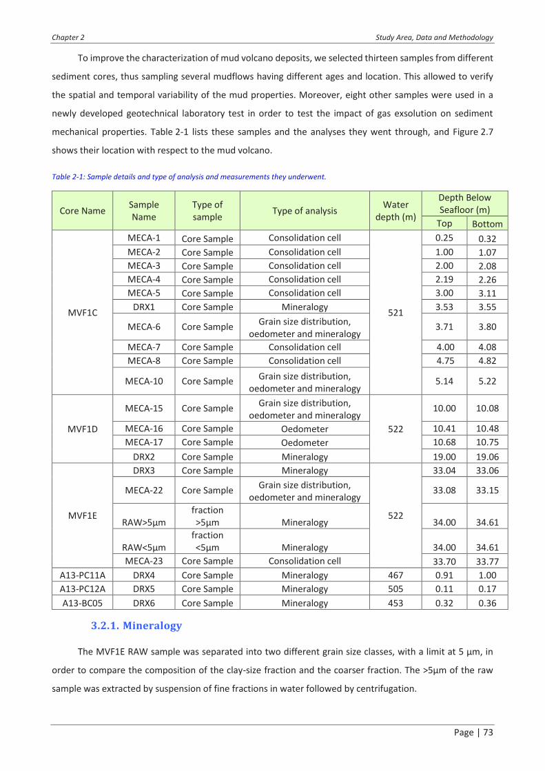
Chapter 2 Study Area, Data and Methodology
Page | 73
To improve the characterization of mud volcano deposits, we selected thirteen samples from different
sediment cores, thus sampling several mudflows having different ages and location. This allowed to verify
the spatial and temporal variability of the mud properties. Moreover, eight other samples were used in a
newly developed geotechnical laboratory test in order to test the impact of gas exsolution on sediment
mechanical properties. Table 2-1 lists these samples and the analyses they went through, and Figure 2.7
shows their location with respect to the mud volcano.
Table 2-1: Sample details and type of analysis and measurements they underwent.
3.2.1. Mineralogy
The MVF1E RAW sample was separated into two different grain size classes, with a limit at 5 µm, in
order to compare the composition of the clay-size fraction and the coarser fraction. The >5!m of the raw
sample was extracted by suspension of fine fractions in water followed by centrifugation.
Core Name Sample
Name
Type of
sample Type of analysis
Water
depth (m)
Depth Below
Seafloor (m)
Top Bottom
MVF1C
MECA-1 Core Sample Consolidation cell
521
0.25 0.32
MECA-2 Core Sample Consolidation cell 1.00 1.07
MECA-3 Core Sample Consolidation cell 2.00 2.08
MECA-4 Core Sample Consolidation cell 2.19 2.26
MECA-5 Core Sample Consolidation cell 3.00 3.11
DRX1 Core Sample Mineralogy 3.53 3.55
MECA-6 Core Sample Grain size distribution,
oedometer and mineralogy 3.71 3.80
MECA-7 Core Sample Consolidation cell 4.00 4.08
MECA-8 Core Sample Consolidation cell 4.75 4.82
MECA-10 Core Sample Grain size distribution,
oedometer and mineralogy 5.14 5.22
MVF1D
MECA-15 Core Sample Grain size distribution,
oedometer and mineralogy
522
10.00 10.08
MECA-16 Core Sample Oedometer 10.41 10.48
MECA-17 Core Sample Oedometer 10.68 10.75
DRX2 Core Sample Mineralogy 19.00 19.06
MVF1E
DRX3 Core Sample Mineralogy
522
33.04 33.06
MECA-22 Core Sample Grain size distribution,
oedometer and mineralogy 33.08 33.15
RAW>5µm
fraction
>5µm Mineralogy 34.00 34.61
RAW<5µm
fraction
<5µm Mineralogy 34.00 34.61
MECA-23 Core Sample Consolidation cell 33.70 33.77
A13-PC11A DRX4 Core Sample Mineralogy 467 0.91 1.00
A13-PC12A DRX5 Core Sample Mineralogy 505 0.11 0.17
A13-BC05 DRX6 Core Sample Mineralogy 453 0.32 0.36

Chapter 2 Study Area, Data and Methodology
Page | 74
The eight samples were analyzed using a reference quantitative mineralogy method called MinEval
QM (Fialips et al., 2018). This method is based on the integration of results from various measurements
performed on crushed samples, including X-Ray diffraction on bulk powders and extracted fine fractions, Loss
On Ignition, X-Ray Fluorescence, Insoluble Residue upon HCl 15% treatment, bulk solid density and Cationic
Exchange Capacity (see Fialips et al. (2018) for more details). This method performs an initial semi-
quantitative mineralogy analysis by Rietveld refinement of the XRD patterns (Rietveld, 1969) and
quantification is completed applying a dedicated software that uses an iterative approach. The <5µm fraction
of MVF1E-RAW only obtained a semi-quantitative mineralogical analysis of clay minerals. The quantity of fine
material obtained after separation was insufficient to perform the complete quantitative study.
3.2.2. Biostratigraphy
A biostratigraphic study was carried out by Chevron in 2000 with the aim of dating the oldest material
present the mudflows. A series of samples were recovered in and around the mud volcano location (green
triangles in Figure 2.7). The samples around the structure were used as age control points. The elements
picked and counted on the samples are diatoms, pollens, foraminifera, nannofossils and ostracods.
Moreover, another analysis of nannofossils was carried out by the Biostratigraphy Dpt. in Total during
the PhD on clasts sampled along sediment cores MVF1 and PC-11A (location in Figure 2.7). The goal was to
verify the age of these cm-sized clasts present within the mud breccia. Foraminifera fauna was also looked
into.
3.2.3. Grain-size distribution
Grain size distribution for the natural mud was determined using the Mastersizer 3000 device for laser
diffraction granulometry (Ryzak & Bieganowski, 2011). This device is a laser diffractometer that measures the
diffraction of a laser beam through water in which solid particles of the mud are suspended. The diffraction
angle and the diffracted beam intensity highly depend on the grain size. The bigger the particle, the smaller
is the diffraction angle and the stronger is the diffracted beam (Ryzak & Bieganowski, 2011). This diffracted
beams are directly analyzed by a dedicated software, which directly gives the results in terms of grain-size
distribution using the Mie solution to Maxwell�s equations that describes the scattering of an electromagnetic
wave by a sphere, whatever the nature of the sphere (Stratton, 1941).
The procedure consists in sampling 1 g of sediment and is mixing it with water and 1 g of sodium
hexametophosphate which helps to deflocculate clay particles (Landrou, Brumaud & Habert, 2016). Samples
are put for 10 minutes into an ultrasound tube in order to break more rapidly potential clay floccules and
then they are mixed into a mechanical stirrer. Afterwards, the content of each bottle is poured into the
diffractometer container that measures the grain-size distribution, and eventually proceeds to auto-cleaning
of its tanks.

Chapter 2 Study Area, Data and Methodology
Page | 75
3.2.4. Mechanical properties of sediments
i. Atterberg Limits
Atterberg limits are the water contents which define transition between different mechanical states
and behaviors of a given sediments (from solid to liquid). The water content corresponds to the ratio between
the mass of water and the mass of the dry sample. The mass of water is obtained by subtracting from the
(wet) sample mass the mass of the same sample after drying during 24 hours in an oven at 105°C. The liquid
limit (wL) is the water content above which sediments stop deforming as a plastic material but start behaving
as fluid (Skempton, 1944; Terzaghi & Peck, 1948). The plastic limit (wp) is the water content below which a
sediment stops deforming as a plastic material and starts to deform as a friable material (Skempton, 1944;
Terzaghi & Peck, 1948). The plasticity index (PI) is obtained by subtracting wP from wL (PI = wL � wP) and
indicates the range of water content where the soil behaves as a plastic material.
In this work, the Atterberg limits were determined using the fall cone method (Figure 2.9;
Feng, 2000, 2005) which consists in dropping vertically a calibrated steel cone (Figure 2.9a) from a position
where the tip is just in contact with the sample surface (Figure 2.9a; Feng, 2005). Feng and co-authors (2005)
showed that the penetration of the cone depends on the water content w and corresponds to 2 mm when
w is equal to the plastic limit and to 20 mm when w is equal to the liquid limit (Figure 2.9b).
Figure 2.9: a: picture of the fall cone test apparatus, displaying the main elements. b: typical log-log diagram of the water content
versus the penetration depth, displaying the reading methods for the Atterberg limits (from Feng, 2005).

Chapter 2 Study Area, Data and Methodology
Page | 76
ii. Odeometer and permeameter tests
Oedometer tests were carried out along with permeability measurements on four samples taken from
the GT1-MVF1 core (MECA 6-10-15-22 in Table 2-1). Tests were duplicated in order to check for potential
trial mistakes. The samples were selected based on Cone Penetration Testing (CPT, location in Figure 2.7;
Lunne 2010) data showing at least four mechanically distinct intervals (Total proprietary report, G. Dan & S.
Po, 12/09/2017, personal communication). The aim of these oedometer tests was to define compressibility
characteristics (void ratio versus effective stress; ASTM International, 1996).
The void ratio e changes are tied to the vertical effective stress s�v by the following compressibility
relation:
! = " !# $ %&log ' ()*
()*+, (1)
where e0 is the initial void ratio for a reference vertical effective stress s�v0 and CC is the compression
index depending on the sediments.
The samples were all reconstituted with an artificial initial water content of around 1.5 wL. Oedometer
tests were conducted using incremental loading (Figure 2.10a) according to the ASTM D-2435 method
(ASTM International, 1996). The remolded sediments are placed into a cell and between two porous stone
plates (Figure 2.10a). The load is applied at the top of the sample through a lever arm (Figure 2.10a). At the
other end of the lever arm, masses are doubled every 24 hours until reaching 32 kg corresponding to a
maximum vertical stress of 1765 kPa. During unloading, the applied mass is divided in half every hour. The
variation in height of the sample is measured using a displacement sensor precise at 0.01 mm (Figure 2.10a).
The initial void ratio e0 of the remolded sample is obtained from the initial water content (w0) using
the following equation:
!# = -#. /0 (2)
Where Gs is specific gravity of soil solids.
Final results of the oedometer test are displayed as variations of e as a function of s�v (Figure 2.10b), e
being obtained at each increment step calculating the sample height variation, DH, and normalizing it with
the initial height, H0, and with e0:
! = " !# $"122+ "34 5"!#6 (3)
From this plot, several sediment mechanical properties can be obtained through graphical methods
(Figure 2.10b). Notably, the compression index, CC, is read directly as the slope of the virgin consolidation
curve (Figure 2.10b) and corresponds to the slope of Eq. (1). The swelling index, CS, is the slope of the swelling

Chapter 2 Study Area, Data and Methodology
Page | 77
curve (Figure 2.10b). Finally, the preconsolidation pressure of sediments is obtained following the graphical
method described by Das (2013) and displayed in Figure 2.10b.
Figure 2.10: a: picture showing one oedometer used during the study, displaying the main elements of the system. b: typical plot for
an odeometer test result after increment load and unload, displaying the consolidation curve, the swelling curve and the virgin
consolidation curve. The method for calculating the preconsolidation pressure (s�P0) and for the reading of the compression index (CC)
and swelling index (CS) is also displayed. A is the maximum inflexion point of the laboratory consolidation curve. From this point, the
tangent to the curve and the horizontal line are drawn. The bisector between these two lines gives the point B at the intersection with
the virgin consolidation curve. The horizontal coordinate of B gives s�P0.
The hydraulic conductivity relation to void ratio is assumed to be:
ln376 = 8! 5 9 (4)
with K the Darcy permeability (Das, 2013) or hydraulic conductivity (m/s), a and b are constants
characteristic of the tested sediments.
The determination of hydraulic conductivities is possible using the falling head method. It consists in
imposing one meter of water head above the oedometer sample and recording the decrease of the water
level over time (Das, 2013). The water head is imposed through infill of capillary (see Figure 2.10a). From the
water head variation we can calculate a hydraulic conductivity (Das, 2013):
7 = 0.:;.< >?@
ABAC
(5)
where s is the surface area of the cross section of the capillary tube (m²), S is the surface area of the
tested sample (m²), L is the length of the tested sample (m), t is the time elapsed since the beginning of the

Chapter 2 Study Area, Data and Methodology
Page | 78
falling head test (s), h1 is the initial level of the water head (m) and h2 is the level of the water head at the
time of the measurement (m).
The calculation of K is repeated at each measurement, and a mean value of K is calculated for each
loading stage, therefore relating a value of K to a given value of e.
In order to artificially characterize the impact of coarse material on mechanical properties, additional
oedometer tests were carried out on grouped MECA-16 and MECA-17 samples (Table 2-1) mixed with a
known mass of fine sand (80-125 µm); the goal was to obtain their compressibility and permeability in order
to integrate these results in numerical diffusion models. The fractions of coarse material added to the
samples were selected based on the �sand / shale ratio� (ratio between sand layer cumulated thicknesses
over total interval thickness) values calculated from well data on different stratigraphic intervals.
iii. Consolidation test with gas exsolution
Figure 2.11: Picture showing the main modules of the special consolidation testing. Details are given in the Chapter 4, dedicated on
the experimental testing program and results.
A novel experimental set-up composed of three main modules was developed to analyze the gassy
sediments and the effects of gas exsolution on the mechanical behavior of compacted sediments
(Figure 2.11). The three modules are: a consolidation cell with a mechanical press designed to apply vertical

Chapter 2 Study Area, Data and Methodology
Page | 79
loads, a saturation module where water is carbonated under a given CO2 gas pressure and the control panel
that connects all the experimental set-up sensors with a computer in order to constrain and record the
different parameters.
The consolidation cell is composed of a Plexiglas cylinder that forms, along with its two end covers, the
fixed part of the system (Figure 2.11). The piston is composed of a steel rod fixed into a pierced plastic
cylinder (Figure 2.11). Two porous stones placed at the top and the bottom of the sample ensure the
consolidation of the sediment during loading by letting water percolate out of the tested sediments. A load
cell and a vertical displacement sensor allow controlling the rate of displacement and the axial force applied
to the sample (Figure 2.11). A lip seal circles the piston and avoids sediments flowing above the piston, with
the adverse effect that it generates a non-negligible friction on the inner surface of the Plexiglas cylinder.
Force balance at the sediment-piston contact shows that the measured force is a composition of the friction,
a vertical upload force due to the different piston surfaces on which fluid pressure is applied (Figure 2.11),
and the net applied load. Friction is always opposed to piston movement. Calibration testing was necessary
in order to constrain the friction related to the asymmetrical lip seal, therefore several tests were made in
water with different gas pressures; the results show that the friction depends on gas pressure and is different
during loading and unloading. Further details on calibration are given in Chapter 4. Details on the different
sensors and structural elements such as Plexiglas cylinder and lip seals are displayed in Table 2-2.
Table 2-2: Sensors and important structural elements characteristics such as measure range and precision or limit pressure.
Sensors and gauges Structural components Load cell Consolidation Cell Cylinder
Maximum load 5 kN Material Plexiglas Maximum vertical stress 1300 kPa Type PMMA XT Precision ± 0.005 kN Elastic Modulus 3.3 Gpa
Displacement sensor Yield Stress 70-80 Mpa Maximum displacement 50 mm Thickness 15 mm Precision ± 0.125 mm Saturation tanks
Pressure gauges Material Plexiglas Limit pressure 3 Mpa Type PMMA XT precision ± 0.75 kPa Limit pressure 1 MPa
CO2 bottle pressure gauge Lip seals max pressure delivery 2.5 Mpa Friction Error ± 0.01 kN
Bender elements
Type GDS Bender System
Limit pressure 3.5 MPa
wave-type S-waves, P-waves
wave shape Sinusoïdal, square
Frequency ranges 0.01-100 kHz
Working frequency 100 kHz
Chapter 2 Study Area, Data and Methodology
Page | 80
The saturation system is composed of two Plexiglas tanks, the same type as the consolidation cell
(Figure 2.11). Both tanks are connected at the top to a CO2 bottle equipped with an adjustable pressure
gauge. Tanks are half-filled with water, the other half being occupied by gas. Adjustable security valves are
connected at the top of the two tanks and allow to expel gas if a pressure threshold is reached (green buttons
in Figure 2.11). Each tank connects to the top or the bottom of the consolidation cell by their bottom end.
Differential pressures at the top and bottom of the sample can be applied through the two tanks allowing
the carbonated water to circulate through the sample, allowing saturating easily the sediments with
dissolved CO2. Pressure gauges control the pore pressure of the system (top and bottom of the consolidation
cell in Figure 2.11). Further technical details on the pressure gauges are displayed in Table 2-2. All the sensors
used (load cell, vertical displacement sensor and pressure gauges) are connected to a control panel
(Figure 2.11). The computer monitors, records and controls the different test parameters.
A pressure generator is connected at the bottom end of the consolidation cell for water permeability
measurements. The pressure generator creates a pressure gradient while measuring water volume change.
Using Darcy�s law, it is possible to calculate the hydraulic conductivity of the sediment. A falling head method
can also be applied using the differential pressure between the two saturation tanks. P-wave velocities are
measured using GDS bender element system. To obtain repeatable and comparable measurements, the
received signal is picked on the last relative minimum before the first received peak. Technical information
on the GDS bender system is given in Table 2-2.
The main purpose of this experimental study is to evaluate the impact of gas exsolution and
accumulation on the mechanical behavior of the tested sediments (e.g. compressibility, preconsolidation
pressure, permeability, P-wave velocity). To do so, several loading/unloading cycles are applied during each
test on water-saturated sediments and gassy sediments. Each test can be described with the following basic
scheme and stages:
· Water saturation with CO2.
· Sample saturation with carbonated water.
· Consolidation/unloading cycle(s) of water-saturated sediments.
· Gas exsolution.
· Consolidation of gassy sediments.
In the case of partial degassing, the last two stages can be repeated to obtain different gas saturations
during the same test. Further details on testing execution can be read in Chapter 4. Gas saturation is
calculated from the volume of gas exsolved, measured by the sample swelling during the exsolution phase.

Chapter 2 Study Area, Data and Methodology
Page | 81
3.3. Well data interpretation
The sand / shale ratio (cumulated sand thickness divided by total interval thickness) was calculated for
each drilled formation based on the lithological, GR and caliper logs (see Chapter 2:2.3.1 and Chapter 2:2.3.6).
Moreover, the ratio between the fracturing pressure and the lithostatic pressure in wells gives a
pressure condition for hydrofracture generation.
In the absence of direct measurements, we estimated interval hydraulic conductivity from the sonic
log using the sonic vs. porosity relationship of Wyllie et al. (1958) and the Kozeny-Carman equation to derive
permeability from porosity (Kozeny, 1927; Carman, 1937).
Wyllie et al. (1958) gave a relationship between measured P wave velocity of a porous media and its
porosity $:
DEF= G
EH5 3DIG6
EJ (6)
with Vm the measured acoustic velocity, Vf the acoustic velocity in pore fluid and Vs the acoustic velocity
in the rock matrix.
As void ratio and porosity are linked through the relation
! = " GDIG (7)
it is possible to calculate hydraulic conductivities K for reservoir layers using the Kozeny-Carman
relationship (Ren et al., 2016):
7 = %K D;J²
LHMNJ²
OP3DQO6" (8)
where CF is a shape constant around 0.2, Ss is the specific surface area of particles (m²/g) taken here as
equal to 0.5 m²/g, %f is the unit weight of pore fluid (N/m3), &s (kg/m3) is the particle mass-density and * is
fluid viscosity (N.s/m²).
Oedometer test results on natural mud were used as a proxy to estimate shale permeability. From the
lithological log, the column was split into reservoirs and shale intervals. Using Eq. (4), (6), (7) and (8), we
calculate for each individual sand and shale strata their hydraulic conductivity K. The arithmetic average of
hydraulic conductivities gives the horizontal hydraulic conductivity (Kh) for the considered stratigraphic
interval while the harmonic average gives its vertical hydraulic conductivity (Kv, Das, 2013). Finally, the ratio
between Kh and Kv was calculated in order to estimate the permeability anisotropy on each interval.

Chapter 2 Study Area, Data and Methodology
Page | 82
3.4. Numerical modeling
3.4.1. 1D sedimentation and pore pressure accumulation
Excess pore pressure can be related to high sedimentation rates, the mechanism of overpressure
generation being called compaction disequilibrium (see Chapter 1:2.5.1.i; Osborne & Swarbrick, 1997; Sultan
et al., 2004; Swarbrick et al., 2002). The sedimentation rates observed in the basin are among the highest
recorded worldwide (see Chapter 2:1.1). Therefore, the modeling work focuses on this sedimentation effect
as a first approach. The SeCoV3 proprietary software of IFREMER (Sultan et al., 2004) allows quantifying the
evolution of pore pressure using a back analysis based on sedimentation rates, compressibility properties
(Eq. (1)) and permeability evolution with void ratio (Eq. (4)). In addition to the equations solved by SeCoV3,
in the present work we use a mesh-update method considering the compressibility of sediments and the
mobile position of the upper boundary (seawater-sediment interface) at each calculation step. For further
details on the methods, used parameters and results of the 1D simulations please read Chapter 3:3.4.1.
3.4.2. Two-dimensional transient-diffusion process: Darcy�s and Fick�s laws
The excess pore pressure generated by sedimentation and calculated using SeCoV3 was considered as
a boundary condition for the 2D Darcy transient flow calculation. The two-dimensional dissipation and
transmission of overpressure is calculated using the 2D diffusion equation given by:
R1SR< = 'R3TUVR1S6RW² 5 R3TUXR1S6
RY² , (9)
with Du(x,y,t) being the overpressure and Dhx and Dhy respectively the horizontal and vertical hydraulic
diffusivities that are calculated directly from the horizontal and vertical hydraulic conductivities Kx and Ky.
In addition to the transmission/diffusion of pore pressure, we considered in the present work the
molecular diffusion of dissolved methane through Fick�s law. Methane diffusion is calculated using a two-
dimensional diffusion equation referred to as Fick�s law (Eq. (10)), which allows for the description of
diffusion of dissolved molecules into a solvent (Crank, 1975):
R&R< = Z& 'R3T[R&6RW² 5 R3T[R&6
RW² , (10)
with C being the dissolved methane concentration, and DC the methane molecular diffusivity of the
porous water. The effect of tortuosity of pores on molecular diffusivity is considered through the porosity of
the sediment as described by Boudreau (1996).
To solve numerically the 2D diffusion equations (Eq. (9) and (10)), a centered explicit finite difference
discretization scheme is used by considering the initial and boundary conditions for pore pressure and
methane concentration.

Chapter 2 Study Area, Data and Methodology
Page | 83
Faults are characterized by their own methane molecular diffusivities creating preferential pathways
or diffusive barriers. As the modeled stratigraphic column is formed by a succession of metric-scale sand
layers and plurimetric shale intervals, a ratio between horizontal and vertical hydraulic conductivities was
integrated based on the results of the hydraulic conductivity calculations at wells (Chapter 2:3.3). This ratio
allows modeling the natural anisotropy of the sedimentary column due to sand-shale successions. A
hydrofracturing condition based on well data interpretation (Chapter 2:2.3.7) is also used: once the ratio
Du/s�v reaches these conditions, fractures are created and propagate in the critical area. The fracture
permeability properties are calculated from the hydraulic conductivity variation with void ratio, defined on
the stratigraphic layer where the fracture creates and from a fracture void ratio defined by the user.
If fractures open in a dissolved-methane saturated area, decrease in Du due to fracture generation
may be sufficient to trigger methane exsolution. Therefore, depending on methane solubility (Brown, 1990;
Duan & Mao, 2006), and depending on the magnitude of the pressure decrease, the software calculates gas
saturation (Sg), and the consequent decrease in preconsolidation pressure of sediments (s�P0) based on the
constitutive law obtained in Chapter 4 from experimental testing.
The software used in order to compute the simulations of this study was developed internally at
Ifremer for this PhD.
3.4.3. P-wave velocity with gas saturation
Helgerud et al. (1999), based on the Biot-Gassman theory and on previous works by Dvorkin
et al. (1999) on elasticity of marine sediments, proposed an effective medium model to predict P-wave and
S-wave velocities in sediments containing free gas and/or gas hydrates based on mineralogy, compressibility
and initial void ratio.
We used this model to draw a chart for predicted P-wave velocity variation with void ratio for different
values of Sg (Chapter 4) in order to compare our P-wave velocity laboratory measurements during
consolidation testing with gas exsolution (Chapter 2:3.2.4.iii). Compressibility of sediments are obtained from
oedometer testing (Chapter 2:3.2.4.ii) and are detailed in Chapter 3:4.2 and in Chapter 4. The average
number of contacts per grain in a bulk unit (called n in the Helgerud et al. (1999) model) was taken as equal
to 4. The mineralogy from XRD measurements (Chapter 2:3.2.1) was simplified into three poles (clays, quartz
and carbonates) as detailed in Chapter 4. The adopted method and the utilization made from Helgerud et
al. (1999) effective medium theory is summarized in Figure 2.12.

Chapter 2 Study Area, Data and Methodology
Page | 84
Figure 2.12: Adopted method to apply the effective medium theory of Helgerud et al. (1999) (modified from Taleb et al., 2018).
3.4.4. Fluid mud dynamics: modelling approach
In order to model the mud flowing towards the surface, a fluid mechanics approach is often adopted
using simplified Navier-Stokes equations (Gisler, 2009; Zoporowski & Miller, 2009; Collignon et al., 2018a).
Navier-Stokes equations are governed by two basic equations. First, for neglected surface tension,
gravity as sole body force and constant viscosity, the momentum equation is given by:
\ RSR< 5 \]". ^^ = "$]_ 5 \@ 5 `#]a^ (11)
where & is the mass-density of the mud (kg/m3), u is the fluid velocity (m/s), g is the the gravity (m/s2),
*0 is the viscosity considered as constant (Pa.s) and p is the fluid pressure (Pa) (Tryggvason et al., 2006).
Secondly, the mass conservation for incompressible fluids is given by:
]. ^ = b (12)
as stated in Tryggvason et al. (2006).
One method for the resolution of this system of equations (Eq. (11) and Eq. (12)) is given by
Tryggvason (2012). The momentum equation is integrated with time by splitting Eq. (11) into a velocity term
and a pressure term, integrated separately. Then, each term of Eq. (11) is discretized using a Finite-Volume
approach where both equations are applied over a small control volume. More details concerning the basic
Navier-Stokes equations and the numerical methods are shown in Tryggvason (2012).
In the present work, we introduce the effect of gas on the mud mass-density through the following
equation:

Chapter 2 Study Area, Data and Methodology
Page | 85
\ = cd4 $ efh\i 5 34 $ c6\0 (13)
Where c is the porosity and \, \i and \0 are respectively the mass-density of mud, water and solid particles.
The density of free gas is considered as being negligible compared to the water-mass density and the mass-
density of the solid particles. The gas solubility and compressibility are also calculated at each time calculation
step using the Boyle�s law and Henry�s law.
4. Conclusion
The Absheron Mud Volcano is located in the South Caspian Basin, a complex area that has recorded
intense tectonic activity since the Creataceous and which is one of the sedimentary basins having recorded
the largest subsidence and sedimentation rates worldwide, notably through the interaction of three paleo-
river deltas. It is also a province of intense O&G activity due to the presence of several mature source rocks
and numerous high-quality regional reservoirs and structural traps in the anticline crests. The SCB is also
known to hold the densest distribution of MVs worldwide. They are related to anticline crests where gas
accumulations are found and their formation seems intimately linked to fold growth.
The Absheron anticline is a gas condensate field with a high strategical and economical interest for
Total, and production may start as soon as 2021. Therefore, a dense and varied dataset was accumulated
over the exploration phase, with notably high resolution industrial geophysical data (3D seismic, 2D seismic,
HR multibeam bathymetry, Sub Bottom Profiler), geotechnical in situ measurements (CPTu), sediment cores
and two exploration wells together with industrial logs. The dataset is very complete, and multidisciplinary,
thus the AMV can be apprehended through different approaches. Its morphology through geophysical
methods can be understood in detail and compared with in situ data and sediment analysis in order to get a
comprehensive model of its formation. The sediments can be laboratory tested through innovative
techniques to understand the mechanical behavior of the mud. Finally, the comprehensive formation model
and the laboratory results can be confronted through numerical models computing several physical and
geological processes. All in all, the AMV is located in an area that gives a unique opportunity to study an
active MV, its morphology, its dynamic and its formation.

Chapter 2 Study Area, Data and Methodology
Page | 86
Page | 87
Chapter 3: Evolution model for the Absheron mud volcano: from in situ observations to numerical modeling
Abstract
The morphology of mud volcanoes (MV) has been extensively studied over the last few decades.
Although recent research has begun to focus on deep processes and structures, little is known about mud
generation mechanisms. This study aims to investigate the feeder system and formation of an active
kilometer-scale MV by relying on a 3-D seismic survey and an in situ dataset on the Absheron anticline (South
Caspian Basin). Seismic data show a depleted area in the Anhydritic Surakhany Formation (ASF), whose
mineralogical composition fits with surface mud. Well data show that the ASF is a succession of evaporitic
beds and low temperature shales near its fracture pressure. Biostratigraphic analysis confirms a Pliocene
origin for the mud, suggesting that the ASF may be the source. Numerical modeling of sedimentation coupled
with laboratory test results and well sonic logs fairly reproduces the observed in situ overpressure trend.
Two-dimensional methane diffusion coupled with overpressure caused by rapid sedimentation highlights the
superposition of critical fracturing conditions with methane-saturated sediments at the base of the studied
MV. This demonstrates the predominant role of fluid overpressure due to sedimentation and gas saturation
in the formation of the Absheron MV, and this is shown to occur as follows: (1) methane migration through
the thrust-related faults reaching the ASF, accompanied by (2) lateral overpressure, caused by rapid
sedimentation, diffusing along the ASF leading to (3) hydro-fracturing of overpressured and methane-
saturated sediments resulting in an important decrease in overpressure, causing (4) gas exsolution and
expansion triggering sediment remobilization.

Page | 88

Page | 89
Chapitre 3 : Mode" le de formation du volcan de boue d�Absheron : des observations in situ au mode" le nume! rique
Résumé
La morphologie des volcans de boue a été étudiée de façon approfondie depuis quelques dizaines
d�années. Bien que les recherches récentes commencent à se concentrer sur les processus et les structures
profondes des volcans de boue, la compréhension des mécanismes de génération de la boue reste partielle.
Cette étude vise à étudier le système profond et la formation d�un volcan de boue actif de quatre kilomètres
de diamètre en se basant sur un bloc de sismique 3D et sur des données in situ couvrant l�anticlinal
d�Absheron (Bassin sud caspien). La sismique permet de mettre en évidence une zone déplétée dans la
Formation du Surakhany Anhydritique (ASF) dont la composition minéralogique s�approche de celle de la
boue du volcan. De plus les données de forage montrent que l�ASF est formé d�une succession de lits
évaporitiques et de bancs argileux, est actuellement proche de sa pression de fracturation et est à une
température bien inférieure à la limitte de remobilisation des argiles. L�analyse biostratigraphique de la boue
permet de confirmer son origine Pliocène. La modélisation numérique de la sédimentation, couplé aux
propriétés mécaniques de la boue et aux diagraphies soniques dans les puits permet de reproduire de façon
assez précise le champ de pression mesuré in situ. La modélisation de la diffusion de pression en deux
dimensions couplé à la diffusion de méthane dissous montre la superposition de surpressions proches des
conditions de fracture et de la zone saturée en méthane dissous sous le volcan actuel. Ce chapitre démontre
l�importance de la surpression générée par une sédimentation rapide ainsi que la présence de gaz dissous
dans la formation du volcan de boue d�Absheron. Le chapitre conclut par le modèle de formation pour ce
volcan le plus probable au vue de l�analyse des données : (1) migration de méthane dissous le long du réseau
de failles se terminant dans l�ASF ; (2) en parallèle, formation d�une zone à forte surpression au niveau de
l�ASF due à la sédimentation rapide dans la partie profonde du bassin ; (3) hydrofracturation des sédiments
en surpression et saturés en méthane dissous induisant une chute rapide de la surpression ;
(4) déclenchement de l�exsolution et expansion du gaz dissous permettant la remobilisation de sédiments.

Page | 90

Chapter 3 Evolution model for the Absheron mud volcano
Page | 91
1. Introduction
Although mud volcano (MV) surface morphologies have been described in detail and worldwide, both
onshore and offshore, little is known about their evolution and formation processes (e.g. Kopf, 2002;
Deville, 2009; Mazzini & Etiope, 2017). On the other hand, earlier extensive work on fluid emissions at the
surface has improved understanding of subsurface processes and the multiple sourcing of the different
elements forming the material ejected by mud volcanoes (Deville, 2009; Kopf, 2002; Mazzini & Etiope, 2017).
Nevertheless, recent technical improvement of geophysical tools, such as high-resolution 3D seismic
imaging, allows for detailed analysis of the MV rooting system and has opened the way for studying mud
generation processes (Stewart & Davies, 2006; Dupuis, 2017; Kirkham et al., 2017a). Understanding these
generation mechanisms is a key issue for geohazard assessment (e.g. the Lusi catastrophe near Sidoarjo,
Indonesia since 2006, Tingay et al., (2015)), for environmental impacts on seabed ecosystems (Zitter, 2004;
Foucher et al., 2009), targeting drilling areas and anchoring zones for offshore infrastructures (Tingay et
al., 2008; Contet & Unterseh, 2015). Furthermore, one characteristic shared by all MVs around the world is
the presence of gas in the ejected material (Hedberg, 1974; Etiope et al., 2009). Yet it is not clear at present
if the gas is a driver of mud extrusion or a passive actor, captured in the mud during its ascent. If gas has a
driving role in mud extrusion, the understanding of mud generation mechanisms could provide elements to
quantify the volume of expelled methane and therefore evaluate the natural contribution of MVs to the
atmospheric carbon budget (Kopf, 2002).
The South Caspian Basin (SCB), along with its onshore continuation, the Lower Kura Basin, is a prolific
hydrocarbon basin and is also known to hold the highest density of MVs (Guliyev et al., 2011; Mazzini &
Etiope, 2017). The Absheron gas field is a challenging exploration and production area due to the presence
of a giant active MV. A high-resolution 3D seismic block was acquired in 1996, two exploration wells were
drilled in 1999 and 2011, and a geotechnical marine survey with sediment core sampling and in situ
measurements was operated in 2014 for geohazard assessment.
Altogether, the dataset provides a rare opportunity to study a mud volcano with a complete set of
surface and subsurface data. Several issues are assessed in this chapter regarding the stratigraphic source of
the mud, the stratigraphic and lateral location of the mud generation zone and the physical mechanisms
responsible for the mud volcano formation.
We provide within this study a detailed geomorphological description of the structure as well as the
extrusion timing based on seismic imaging and other data. Well data and sediment analysis results were
integrated into numerical 1D and 2D models in order to quantify the lateral pressure transmission and the
gas migration effect. Finally, a conceptual evolution model based on these results is proposed.
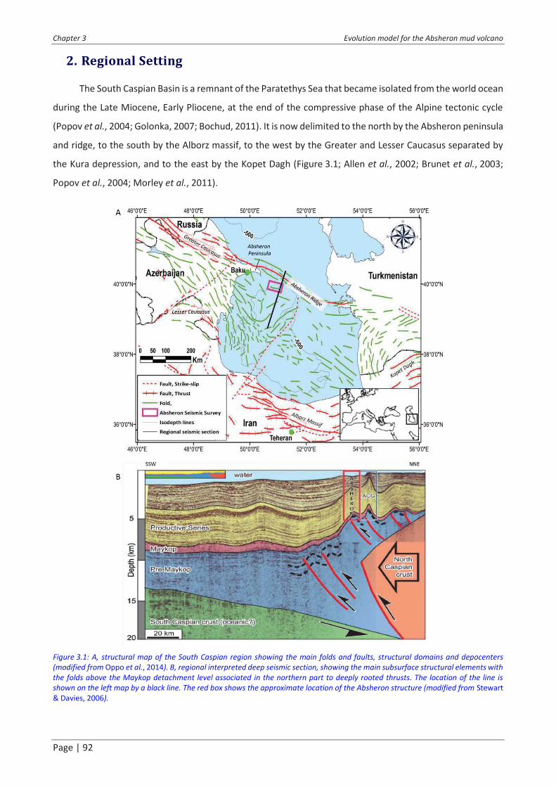
Chapter 3 Evolution model for the Absheron mud volcano
Page | 92
2. Regional Setting
The South Caspian Basin is a remnant of the Paratethys Sea that became isolated from the world ocean
during the Late Miocene, Early Pliocene, at the end of the compressive phase of the Alpine tectonic cycle
(Popov et al., 2004; Golonka, 2007; Bochud, 2011). It is now delimited to the north by the Absheron peninsula
and ridge, to the south by the Alborz massif, to the west by the Greater and Lesser Caucasus separated by
the Kura depression, and to the east by the Kopet Dagh (Figure 3.1; Allen et al., 2002; Brunet et al., 2003;
Popov et al., 2004; Morley et al., 2011).
Figure 3.1: A, structural map of the South Caspian region showing the main folds and faults, structural domains and depocenters
(modified from Oppo et al., 2014). B, regional interpreted deep seismic section, showing the main subsurface structural elements with
the folds above the Maykop detachment level associated in the northern part to deeply rooted thrusts. The location of the line is
shown on the left map by a black line. The red box shows the approximate location of the Absheron structure (modified from Stewart
& Davies, 2006).

Chapter 3 Evolution model for the Absheron mud volcano
Page | 93
Since the Middle Miocene, compression uplifted all these massifs and triggered the high amplitude
folding of the South Caspian sedimentary series (Allen et al., 2002; Popov et al., 2004; Egan et al., 2009;
Javanshir et al., 2015). This compression initiated the subduction of the South Caspian basement below the
basement of the North Caspian domain, creating the Absheron ridge in-between (Figure 3.1; Allen et
al., 2002; Stewart & Davies, 2006). The subduction allowed the deposition of more than 8 km of sediments
over the last 5.5 Ma based on a representative stratigraphic column of the northwestern part of the basin,
which is faster than sedimentation rates recorded in typical foreland basins (Allen et al., 2002; Stewart &
Davies, 2006; Morley et al., 2011).
The Maykop Formation was deposited from the Late Oligocene to the Early Miocene in a shallow
marine anoxic environment (Popov et al., 2004; Golonka, 2007; Hudson et al., 2008). It is the main
hydrocarbon source rock for the Caspian and Black Sea areas (Allen et al., 2002; Hudson et al., 2008) and acts
as the main decollement level for the high amplitude folds of the South Caspian Basin (Allen et al., 2002;
Stewart & Davies, 2006). The Maykop sediments are mainly organic-rich clays with a minor fraction of coarser
detrital material (Hudson et al., 2008).
Post-Maykop Miocene sediments were deposited in a context of global regression until basin isolation
occurred in the Late Miocene. These sediments are shallow marine and lacustrine thick clayey deposits (Allen
et al., 2002; Javanshir et al., 2015).
The Pliocene was dominated by deltaic and lacustrine environments during a regression phase, fed
from the ancestral Kura, Volga and Amu-Darya rivers that drained sediments from all the topographic highs
surrounding the basin (Allen et al., 2002; Abdullayev & Leroy, 2016). The subduction-related subsidence at
the end of the Miocene accommodated the deposition of thick deltaic deposits forming the regional
hydrocarbon reservoirs (Allen et al., 2002; Javanshir et al., 2015). The sedimentation rate was very high,
reaching 2.4 km/Ma, with up to 6 km of the Productive Series (PS) (Allen et al., 2002; Brunet et al., 2003;
Stewart & Davies, 2006). At the top of the Surakhany Formation (Upper PS), the regression was maximal and
evaporitic beds are found in the northern part of the basin (Javanshir et al., 2015). This interval will hereafter
be called Anhydritic Surakhany.
Above the Productive Series, the Akchagyl Suite consists of open marine mudstones. This transgressive
interval records the temporary reconnection of the SCB to the world ocean from 2.4 to 1.6 Ma (Allen et
al., 2002; Javanshir et al., 2015; Dupuis, 2017). From 1.6 Ma to present, deep-water lacustrine and brackish
conditions have dominated, forming the Absheron Suite and younger units.
More detailed information on the stratigraphy of the South Caspian Basin is given in Chapter 2:1.1.2
and is synthesized in Figure 2.4.

Chapter 3 Evolution model for the Absheron mud volcano
Page | 94
The presence of the high TOC (Total Organic Carbon) Maykop Formation and of the well-connected PS
reservoirs make the SCB a prolific hydrocarbon basin (Hudson et al., 2008; Javanshir et al., 2015; Alizadeh et
al., 2017). The Maykop Formation generates gas in the deeper part of the basin and is still generating oil
onshore and in the northern margin of the basin (Figure 2.6; Javanshir et al., 2015). Large-scale anticlines (50-
150 km long), detached over the overpressured and under compacted Maykop formation (Morley et
al., 2011) form excellent oil and gas traps as hydrocarbons migrate from the deep basin into the onshore
heights along the regionally continuous reservoirs (Javanshir et al., 2015). The large-scale anticlines main
growth stage occurred at the end of Pliocene. However, fold-growth is ongoing although slower (Mosar et
al., 2010).
One hundred and eighty active MV�s are listed onshore, and at least the same amount is estimated in
the offshore part of the SCB (Milkov, 2000; Guliyev et al., 2001; Kopf, 2002; Mazzini & Etiope, 2017). These
structures are mainly located along the crests of anticlines where oil and gas have accumulated in reservoirs
(Deville, 2009; Javanshir et al., 2015; Mazzini & Etiope, 2017). They are generally considered to be sourced
by the Maykop Formation (Kopf, 2002; Stewart & Davies, 2006; Roberts et al., 2010). Additionally, Fowler et
al. (2000) noticed on the offshore Shah Deniz anticline a close relationship between the development of folds
and mud volcano activity as mud volcanoes activated during or after fold initiation and the authors correlate
structural growth with mud volcano activity phases.
The Absheron anticline is a NW-SE oriented, 40 km-long fold, located at the northwestern edge of the
SCB, 100 km to the south-west of Baku and 50 km south of the ACG gas-field (Figure 3.1A). Methane was
recently discovered in the Absheron field and a giant active mud volcano pierces the crest of the structure at
the southwestern limit creating potential hazards for drilling operations. Previous studies on the Absheron
anticline evidenced the presence of four mass transport deposits (MTDs) in the Post-Absheron interval
(Imbert et al., 2014). The most recent MTD covers the whole anticline with the exception of the mud volcano
location where it stumbles on the northern flank of the volcano. Morphology of the mud volcano in the upper
500 m of the sediment pile is described in Dupuis (2017). The poorly imaged central part is surrounded by
three stacked wedges affected by multiple thrusts. Recent activity of the mud volcano is confirmed by four
mudflows imaged in the first 100 m below seafloor (mBSF).
3. Materials and methods
3.1. Seismic data
This study focuses on the Absheron anticline, where an active mud volcano is imaged by a 3D seismic
survey (limits and location on Figure 3.1). The seismic survey covers 650 km², in water depths ranging from
180 to 700 m. The seismic sections presented here are from Kirchhoff pre-stack time migration (PSTM)
processing and from Kirchhoff pre-stack depth migration (PSDM) reprocessing (Robein, 2010), which was

Chapter 3 Evolution model for the Absheron mud volcano
Page | 95
applied on 550 km² of the seismic survey. The velocity model used in the reprocessing aimed to improve the
imaging of the deep structures (thrust, dips), taking into account the lateral velocity variations across the
thrust as well as the velocity heterogeneity in the shallow intervals due to the presence of the mud volcano
and free gas (Adler, 2018, pers. com.). The model parametrization is a vertical transverse isotropy (VTI) that
considers the vertical anisotropy imposed by the sedimentary strata (Robein, 2010). The model was entirely
built by tomography inversion (Robein, 2010), and in the deep part, it was corrected using an interpretative
method in order to preserve the structural coherency and to fit the well data (Adler, 2018, pers. com.). The
seismic volume is composed by 2203 inlines and 2120 crosslines with 12.5 m spacing inline and 18.5 crossline.
The vertical resolution varies with depth as it depends on interval velocity. From visual observations of the
sections, we estimate a resolution ca. 20 m in the strata above 2000 m, progressively decreasing to 150 m at
11 km.
Each medium has its own acoustic impedance. Therefore, when a seismic signal reaches a limit
between two media with different impedances, part of the acoustic signal will be reflected (Nely, 1986). A
seismic signal can be decomposed in wavelets which are characterized by their polarity, their amplitude (peak
area), its period and its phase (Nely, 1986). Normal polarity is given by the seafloor polarity, which in the data
presented hereafter is a wavelet with a strong central positive amplitude surrounded by two weak negative
amplitudes. Thus, the normal polarity is a strong positive peak enclosed between two weak negative peaks
indicating a step-wise increase in impedance. The opposite shows a step-wise decrease in impedance
(Nely, 1986; Ricker, 1953).
Seismic interpretation was carried out using the Total in-house software Sismage (Guillon &
Keskes, 2004). From the 3D seismic cube, we calculated the seismic coherency attribute , which can be
projected on horizontal slices or seismic horizons. Seismic coherency allows to laterally differentiate
continuous areas (undisturbed deposits) from low continuity zones (faults or mud volcano deposits for
instance) (Bahorich & Farmer, 1995). Horizons were propagated and named according to stratigraphic limits
encountered in the two exploration wells drilled on the Absheron anticline (Figure 3.2 for location). These
stratigraphic limits are interpreted based on cuttings analysis and gamma-ray, sonic and resistivity logs (see
Chapter 2:2.3). Between two horizons, it is possible to extract layers of regular thickness on which the Root
Mean Square (RMS) of the seismic amplitude can be calculated. This allows visualizing in map view the spatial
distribution of sediment bodies whose impedance contrasts with the background, thus imaging for instance
channels, mudflows, and pipes.
The presence of free gas is a well-documented cause of attenuation or data wipe-out (Graue, 2000;
Benjamin & Huuse, 2017). Mud volcanoes are known to be accompanied by large emissions of gas
(Kopf, 2002; Mazzini & Etiope, 2017). Therefore, seismic masking is expected to occur below large structures
such as the Absheron mud volcano (Graue, 2000; Benjamin & Huuse, 2017). Imaging issues that cannot be
settled by migration algorithms may arise from steep dips (Day-Stirrat et al., 2010).

Chapter 3 Evolution model for the Absheron mud volcano
Page | 96
In parallel of the seismic imaging, high-resolution bathymetric maps (Figure 3.2) were acquired using
a multi-beam echosounder.
Figure 3.2: Seismic amplitude map of the seafloor around the Absheron mud volcano. In orange, a high amplitude mudflow is imaged
to the west of the volcano. The dark patch corresponds to the shield composing the mud volcano itself. On the same map, the location
of the different coring and drilling sites are shown. Limits and location of the 3D seismic survey are presented on the regional map of
the SCB (Figure 3.1A). Red lines indicate the location of the seismic lines presented in Figure 3.3, Figure 3.4 and Figure 3.5. The dotted
black polygone is the limit of the zoom shown below, presenting a detailed image of the seafloor on and around the mud volcano
acuired with a multi-beam echo sounder. Orange stands for the shallower areas, green is for the deeper parts.
3.2. Sediment cores and geotechnical analysis
3.2.1. Sample collection
A marine geological and geotechnical survey of the seabed above the Absheron gas discovery
was carried out in 2014 in order to better constrain and delineate geological hazards associated with the mud
volcano (Total proprietary report, Dan & Po, 2017, pers. com.). The geotechnical/geological survey used
rotary drilling, AUV (Autonomous Underwater Vehicle) sampling with box corer and piston corer as well as in
situ geotechnical testing (Cone Penetration Testing). Well logging and CPT were performed on two boreholes:

Chapter 3 Evolution model for the Absheron mud volcano
Page | 97
CH2 was located outside the mud volcano area to provide a stratigraphic reference in continuous series, and
MVF1 sampled on a mud volcano flow (for location see Figure 3.2).
To improve the characterization of mud volcano deposits, we selected thirteen samples from different
sediment cores. Table 2-1 lists the coordinates and depth below seabed of these samples (all samples
mentioned in Table 2-1, except samples that underwent consolidation testing) and Figure 3.2 shows their
location with respect to the mud volcano. The samples were selected to provide information on the spatial
and temporal variability of the mud volcano deposit (Total proprietary report, Dan & Po, 2017, pers. com.).
Five samples were selected at three different depths from the same rotary drilling cores MVF1, thus
potentially on different mud eruption episodes. One sample from A13-PC12a core was taken from the same
mudflow as the one drilled by MVF1 but at a different location. A different mudflow was sampled on the
A13-PC11a core at the northern edge of the mud volcano. Finally, a sample was taken from the A13-BC05
core directly on the top of the mud shield (see Table 2-1 for further details and Figure 3.2 for location).
3.2.2. Mineralogical and biostratigraphic analysis of the mud
The MVF1E RAW sample was separated into two different grain size classes, with a limit at 5 µm, in
order to compare the composition of the clay-size fraction and the coarser fraction. The >5!m of the raw
sample was extracted by suspension of fine fractions in water followed by centrifugation.
The eight samples were analyzed using a reference quantitative mineralogy method called MinEval
QM (Fialips et al., 2018). This method is based on the integration of results from various measurements
performed on crushed samples, including X-Ray diffraction on bulk powders and extracted fine fractions, Loss
On Ignition, X-Ray Fluorescence, Insoluble Residue upon HCl 15% treatment, bulk solid density and Cationic
Exchange Capacity (see Fialips et al. (2018) for more details). This method performs an initial semi-
quantitative mineralogy analysis by Rietveld refinement of the XRD patterns (Rietveld, 1969) and
quantification is completed applying a dedicated software that uses an iterative approach. The <5µm fraction
of MVF1E-RAW only obtained a semi-quantitative mineralogical analysis of clay minerals. The quantity of fine
material obtained after separation was insufficient to perform the complete quantitative study.
Furthermore, a biostratigraphic study by Chevron in 2000 was carried out with the aim of dating the
oldest material composing the mudflows. A series of samples were recovered in and around the volcano
location (green triangles in Figure 3.2). The samples around the structure were used as age control points.
The elements picked and counted on the different samples are diatoms, pollens, foraminifera, nannofossils
and ostracods.
Initial grain size distribution for the natural mud was determined using the Mastersizer 3000 device
for laser diffraction granulometry (Ryzak & Bieganowski, 2011).

Chapter 3 Evolution model for the Absheron mud volcano
Page | 98
3.2.3. Geotechnical analysis of the mud
Oedometer tests with permeability measurements were carried out on four samples taken from the
GT1-MVF1 core (MECA 6-10-15-22 in Table 2-1 and tests from 1 to 8 in Table 3-1). Tests were duplicated in
order to check for potential trial mistakes. The samples were selected based on Cone Penetration Testing
(CPT, Das (2013)) data showing at least four mechanically distinct intervals (Total proprietary report, Dan &
Po, 2017, pers. com.). The aim of these oedometer tests was to define compressibility characteristics (void
ratio versus effective stress) and to determine the relationship between hydraulic conductivity and void ratio
of the considered sediment intervals (ASTM International, 1996).
Table 3-1: Details on sample preparation for oedometer tests and results.
Test
number Sample
s'vmax
(kPa) wL e0 CC
Sample
Preparation
1 MECA-6 1765.12 0.42 1.95 0.35 1.5 wL water input
2 MECA-22 1765.12 0.43 1.7 0.34 1.5 wL water input
3 MECA-10 1765.12 0.56 2.11 0.42 1.5 wL water input
4 MECA-15 1765.12 0.44 1.79 0.32 1.5 wL water input
5 MECA-6 1765.12 0.42 2.23 0.36 1.5 wL water input
6 MECA-22 1765.12 0.43 1.9 0.33 1.5 wL water input
7 MECA-10 1765.12 0.56 2.58 0.46 1.5 wL water input
8 MECA-15 1765.12 0.44 2.18 0.34 1.5 wL water input
9 MECA-16+17 + 5% sand 1765.12 0.44 1.38 0.25
1.5 wL water input,
mixed samples
10 MECA-16+17 + 10% sand 1765.12 0.44 1.23 0.23
1.5 wL water input,
mixed samples
11 MECA-16+17 + 25% sand 1765.12 0.44 1.14 0.20
1.5 wL water input,
mixed samples
The void ratio e changes is tied to the vertical effective stress s�v by Eq. (1) (Chapter 2:3.2.4.ii). e0 and
CC for the tested samples are shown in Table 3-1. The permeability is linked to void ratio following Eq. (4)
(Chapter 2:3.2.4.ii).
The samples were all reconstituted with an artificial initial water content of around 1.5 wL (wL being
the liquid limit). The wL (Table 3-1) was determined using the fall cone method (Feng, 2005). Oedometer tests
were conducted using incremental loading according to the ASTM D-2435 method (ASTM
International, 1996). The determination of hydraulic conductivities and permeability coefficients was also

Chapter 3 Evolution model for the Absheron mud volcano
Page | 99
possible using the falling head method. Using an exponential regression on the obtained measurements is
necessary to obtain a law of the form of Eq. (4).
In order to artificially characterize the impact of coarse material on mechanical properties, additional
oedometer tests were carried out on grouped MECA-16 and MECA-17 samples (Table 2-1 and Table 3-1)
mixed with a known mass of fine sand (80-125 µm); the goal was to obtain their compressibility and
permeability in order to integrate these results in the numerical diffusion model. The fractions of coarse
material added to the samples were selected based on the net to gross (ratio between sand layer cumulated
thickness over total interval thickness) values calculated from well data.
Further details on the measurements and analysis methods are given in Chapter 2:3.2.4.
3.3. In situ well data and hydraulic conductivity calculations
Stratigraphic information was obtained from the two exploration wells drilled on the Absheron
anticline (Figure 3.2). Well A reached 6506 m TVD/MSL (true vertical depth below mean sea level) whilst Well
B reached 6823 TVD/MSL.
Lithology is obtained from cuttings analysis. Pore pressures in shales were estimated from sonic data
using Eaton�s method (Eaton, 1975). Sonic logs were acquired either with wireline or logging while drilling
(LWD) tools depending on the interval. The StethoScope pressure-while-drilling tool (Schlumberger, 2019)
was used to measure in situ reservoir pore pressure. Fracturing pressure log is evaluated from leak-off tests
(LOT) or formation integrity tests (FIT) (Lin et al., 2008), as well as down hole mud losses. Wireline tools
measured temperatures at different points either in open hole or cased hole.
The sonic measurements are given as slowness of the acoustic waves, e.g. the inverse of acoustic
velocity, which is linked to the porosity of the logged sedimentary interval using Wyllie et al., (1958)
relationship given in Eq. (6) (Chapter 2:3.3). The void ratio and porosity are linked by Eq. (7) (Chapter 2:3.3),
thus allowing calculating hydraulic conductivities K for reservoir layers using the Kozeny-Carman relationship
given in Eq. (8) (Chapter 2:3.3).
Therefore, it is possible to estimate the hydraulic conductivity of reservoirs directly from acoustic log
data. Oedometer test results on natural mud allowed calculation of permeability in the shales. From the
lithological log, the column was split into reservoirs and shale intervals. Using Eq. (4), (6), (7) and (8), we
calculate for each defined interval the hydraulic conductivity K. The net to gross ratio (cumulated sand
thickness divided by total interval thickness) was calculated for each drilled formation. The arithmetic
average of hydraulic conductivities gives the horizontal hydraulic conductivity for the considered formation
while the harmonic average gives its vertical hydraulic conductivity (Das, 2013).
Further details are given in Chapter 2:3.3.

Chapter 3 Evolution model for the Absheron mud volcano
Page | 100
3.4. Numerical modeling: sedimentation, transient pore pressure and gas
diffusion
3.4.1. 1D sedimentation and pore pressure accumulation
Geological formations remain at hydrostatic pressure after deposition and burial as long as pore fluids
are able to escape up through the overburden or laterally towards the seabed or surface. High permeabilities
or low sedimentation rates help pore water escaping during consolidation. In contrast, when permeability is
low or sedimentation rate is high enough, fluids cannot escape fast enough to keep hydrostatic conditions.
As loading increases through sedimentation, pore water starts to support part of the overburden pressure,
which prevents pores from closing. Thus, normal consolidation is delayed, sediments become under-
compacted and pore pressure increases above hydrostatic conditions. This excess pore pressure is called
overpressure and this mechanism of overpressure buildup is called compaction disequilibrium (Osborne &
Swarbrick, 1997; Swarbrick et al., 2002; Sultan et al., 2004).
In this work, we calculate in one dimension the overpressure generated (Du) only by sedimentation
effect in the southern part of the considered section where the sedimentary column is the thickest. The high
sedimentation rates observed in the basin are within the strongest recorded worldwide (Allen et al., 2002;
Brunet et al., 2003; Stewart & Davies, 2006). Moreover, high sedimentation rates are considered to be one
of the main overpressure generation mechanism (Osborne & Swarbrick, 1997; Swarbrick et al., 2002).
Therefore, the modeling work focuses on this sedimentation effect as a first approach. The SeCoV3
proprietary software of IFREMER (Sultan et al., 2004) allows quantification of the evolution of pore pressure
using a back analysis based on sedimentation rates, compressibility properties (Eq. (1), Chapter 2:3.2.4.ii) and
permeability evolution with void ratio (Eq. (4), Chapter 2:3.2.4.ii). In addition to the equations solved by
SeCoV3, in the present work we use a mesh-update method considering the compressibility of sediments
and the mobile position of the upper boundary (seawater-sediment interface) at each calculation step.
Sedimentation rates and the model geometry used in this study were calculated using present
thicknesses and ages from Green et al. (2009). These sedimentation rates have been corrected
(decompression) for compaction using Terzaghi compaction equations (Terzaghi, 1943). At the end of
sedimentation and compaction modeling, we applied a trial and error method until the model matched
present-day observed thicknesses.
Compressibility and permeability properties characterizing each of the defined layers were determined
based on oedometer and permeability tests (Table 3-1) carried out on natural mud mixed with known
fractions of very fine sand (ASTM International, 1996). The fractions of added sand were selected thanks to
net to gross values calculated from well data (Table 3-2). The purpose was to model the behavior of layers
having different amounts of coarser material.

Chapter 3 Evolution model for the Absheron mud volcano
Page | 101
Table 3-2: Results of hydraulic conductivity calculations based on sonic-log data and oedometer tests on natural mud. NTG is the net
to gross, being the ratio between total sand thickness over total interval thickness. The mean void ratio is calculated from the sonic
log (equation (3)) and Kh (horizontal hydraulic conductivity) and Kv (vertical hydraulic conductivity) result respectively from arithmetic
and harmonic average of calculated hydraulic conductivities on individual sand or shale layers using equation (5). The 1D-
sedimentation model gives a range of void ratio for each stratigraphic interval, corresponding to hydraulic conductivity ranges on
oedometer test results obtained for different sand fraction content (Table 3-1). Measured and calculated Ks are in the same ranges of
magnitude.
Layer Name
Layer
number in
model
NTG
(%)
Mean
void ratio
from logs
Kh (m/s) Kv (m/s) Kh/Kv
Void ratio
ranges from
1D-model
K ranges
from
oedometer
tests (m/s)
model
kx/ky
Novocaspian
- Absheron Layer 5 5 0.33 5.03E-07 2.27E-10 2212 2.73 - 0.36
5.01E-07 -
3.53E-10 2200
Surakhany Layer 4 8 0.18 3.18E-09 2.13E-10 15 0.43 - 0.24 7.50E-10 -
4.17E-10 15
Sabunchy Layer 3 12 0.14 1.27E-09 1.95E-10 6 0.22 - 0.21 4.70E-10 -
4.56E-10 6
Balakhany -
Fasila Layer 2 24 0.17 5.16E-10 2.57E-10 2 0.27 - 0.24
7.78E-10 -
7.05E-10 2
NKG Layer 1 8 0.17 2.18E-10 2.10E-10 1 0.24 - 0.22 4.17E-10 -
3.92E-10 1
3.4.2. Two-dimensional transient-diffusion process: Darcy�s and Fick�s laws
The two-dimensional transient dissipation of excess pore pressure generated by the sedimentation
process is considered along a 63-km-long and 10-km-thick block of the section presented in Figure 11 of
Green et al. (2009). We defined the geometrical model with 300 horizontal and 50 vertical nodes by
considering six stratigraphic layers, the fault network around the Absheron fold and normal faults at the
extrados of the fold.
The excess pore pressure generated by sedimentation and calculated using SeCoV3 was considered as
a boundary condition for the 2D Darcy transient flow calculation. The two-dimensional dissipation and
transmission of overpressure is calculated using the 2D diffusion equation given in Eq. (9) (Chapter 2:3.4.2).
Dhx and Dhy, respectively the horizontal and vertical hydraulic diffusivities are calculated directly from the
horizontal and vertical hydraulic conductivities Kx and Ky (Table 3-2).
In addition to the transmission/diffusion of pore pressure, we considered in the present work the
molecular diffusion of dissolved methane. Methane diffusion is calculated using a two-dimensional diffusion
equation referred to as Fick�s law (Eq. (10), Chapter 2:3.4.2), which allows for the description of diffusion of
dissolved molecules into a solvent (Crank, 1975).
To solve numerically the 2D diffusion equations (Eq. (9) and (10), Chapter 2:3.4.2), a centered explicit
finite difference discretization scheme is used by considering the initial and boundary conditions for pore
pressure and methane concentration.
Faults are characterized by their own methane molecular diffusivities creating preferential pathways
for methane. Moreover, as the modeled stratigraphic column is formed by a succession of metric-scale sand
layers and plurimetric shale intervals, a ratio between horizontal and vertical hydraulic conductivities was

Chapter 3 Evolution model for the Absheron mud volcano
Page | 102
integrated based on the results of the hydraulic conductivity calculations at wells (Table 3-2). This ratio allows
modeling of the natural anisotropy of the sedimentary column due to sand-shale successions.
3.4.3. Hydrofracturing
In some cases, excess pore pressure can exceed the effective least principal stress plus the tensile
strength of the medium allowing hydrofracturing to occur (Alfaro & Wong, 2001). When sediments are only
submitted to the load of the overlying sedimentary cover, the greatest effective stress is vertical (s"v) whereas
the least effective stress is horizontal (s"h) (Sibson, 2003). Fractures then open in the direction of the least
principal stress and propagate in the direction of the plane perpendicular to the least principal stress
(Hubbert & Willis, 1957). Therefore, in the case of sole loading effects, hydrofractures will propagate
vertically.
The vertical effective stress and excess pore pressure are an output of 2D Darcy�s diffusion equation.
The ratio between fracturing pressure and overburden pressure (lithostatic stress) observed in the well
ranges between 0.83 and 0.99, with an average of 0.9. Consequently, we consider in the present work that
hydrofracturing will occur whenever the ratio between excess pore pressure and vertical effective stress
(Du /s�v) exceeds 0.9.
4. Results
4.1. Geomorphological investigation of the Absheron mud volcano
Figure 3.3 and Figure 3.4 present two parallel SSW-NNE sections. Figure 3.3 runs across the axis of the
Absheron fold in the vicinity of the two exploration wells drilled on the anticline and Figure 3.4 cuts through
the center of the Absheron mud volcano as located on Figure 3.2. The ages of five of the seismic horizons
that are presented in this study were calibrated from the stratigraphic results of the well (Total proprietary
data). We were able to map the top of Absheron Suite, the top of the Akchagyl Suite, the top of the Productive
Series, the top of the Anhydritic Surakhany Formation, the Top Diatom Suite and the top of the Maykop Suite
(see Figure 2.4 for the stratigraphic column). Seven other seismic horizons were interpreted in order to
highlight particular structures such as normal faults or the morphology of the fold.
The deep part of the Absheron fold is cut by a deep E-W trending thrust that dies out in the Diatom
Suite. This thrust has more than 2 km of throw and the northern block overrides the southern block. The
thickening of the interval between Top Diatom and Top Maykop is interpreted as the result of a backthrust
system that would have been inverted later during its history. Another thrust 5 km to the NNW has a throw
of less than 1 km (Figure 3.3). The main thrust is responsible for the formation of the Absheron fold and
several folding phases can be distinguished. The Productive Series interval has a rather uniform thickness of
5 km
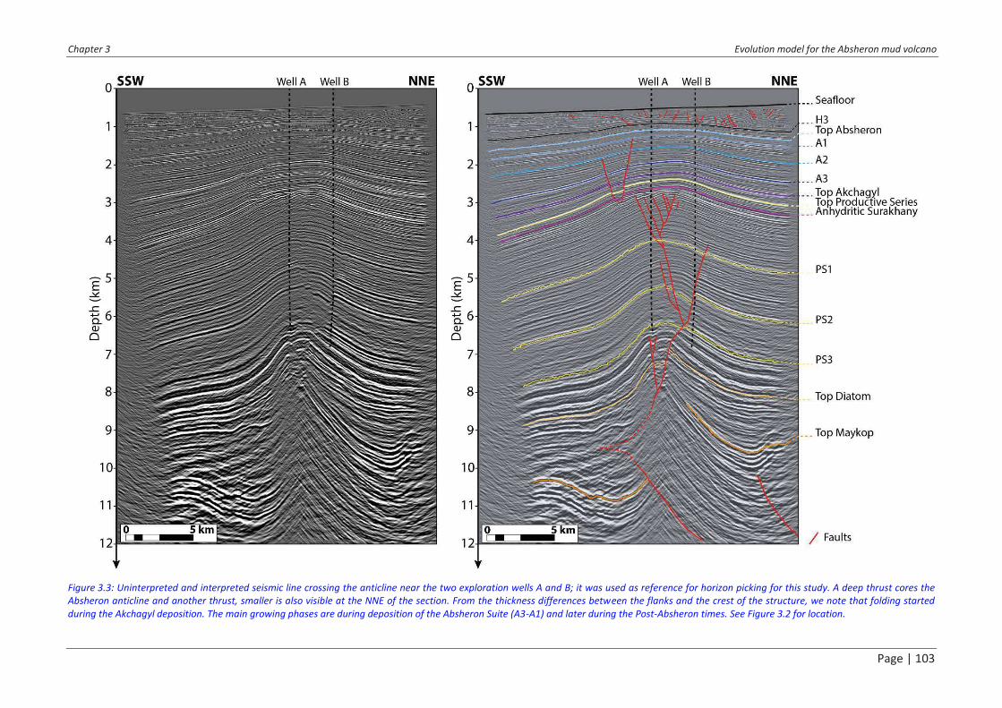
Chapter 3 Evolution model for the Absheron mud volcano
Page | 103
Figure 3.3: Uninterpreted and interpreted seismic line crossing the anticline near the two exploration wells A and B; it was used as reference for horizon picking for this study. A deep thrust cores the
Absheron anticline and another thrust, smaller is also visible at the NNE of the section. From the thickness differences between the flanks and the crest of the structure, we note that folding started
during the Akchagyl deposition. The main growing phases are during deposition of the Absheron Suite (A3-A1) and later during the Post-Absheron times. See Figure 3.2 for location.

Chapter 3 Evolution model for the Absheron mud volcano
Page | 104
across the anticline with only 10% of total thinning from the flanks to the crest of the anticline, indicating a
rapid deposition during a phase of low-activity for the fold (Figure 3.3). The Akchagyl Suite above presents a
thickening towards the southern flank of the fold of 300 m, corresponding to 60% of its maximum thickness
(Figure 3.3), thus indicating that growth of the anticline was accelerated during deposition of this interval.
Fold activity was still strong during deposition of the Absheron Suite as the thinning at the crest reaches 650
m for this interval, 35% of its maximum thickness. More precisely, the interval between horizons A3 and A2
recorded a thinning of 330 m (45% of maximum thickness), and between A1 and A2, 190 m (40% of maximum
thickness, Figure 3.3). More recently, during Post-Absheron times, the fold re-activated and another 450 m
of thinning (45% of maximum thickness) is visible from Top Absheron horizon to the seafloor (Figure 3.3).
Therefore, sediment thinning at the crest of the anticline indicates that fold activity really started at the
Akchagyl times, when it reached its climax. During the Absheron Suite deposition, the fold activity was
intense for a longer time interval, and recent intense fold activity was also recorded in the Post Absheron
interval.
Besides, normal faults on the extrados of the fold form a complex network from the thrust up to the
Upper Productive Series (Figure 3.3). The back thrust was then inverted to form the main observed normal
fault.
The Absheron mud volcano (AMV) is located in the SE part of the 3D seismic survey. Figure 3.2 shows
the seismic amplitude of the seafloor horizon, with a color-scale set to outline high and low amplitude zones.
Orange stands for the highest amplitude and darker areas correspond to lower amplitude zones. The high-
resolution bathymetric map (Figure 3.2) reveals present seafloor morphology related to recent mud volcano
activity. Near surface morphology of the mud volcano was already detailed by Dupuis (2017), with the
presence of three main wedges (�Transparent Facies� and �Chaotic Facies� on Figure 3.4) and at least four
recent mud flows evidenced on seismic data.
This mud volcano is a subcircular mud shield, 4 to 5 km in diameter (Figure 3.3). It is surrounded by a
gently-dipping apron (average outward slope from 4° to 6°), the relief above the surrounding seafloor does
not exceed 70 meters (Figure 3.2). The highest area is a relatively flat plateau, but at a closer look reveals at
least four gently mounded circular structures, 0.5 to 1 km diameter (Figure 3.2); we interpret these as the
loci of most recent mud emission. At the western edge of the mud shield, a 12-km-long, 1.5 to 3-km wide
high-amplitude patch extends from the volcano to the west before following the natural slope towards the
south of the Absheron seismic survey (Figure 3.2). This high-amplitude patch was already described as a giant
mudflow by Dupuis (2017). This mudflow shows up strongly on seabed amplitude maps, indicating that is
closer to seabed than the resolution of the dataset.

Chapter 3 Evolution model for the Absheron mud volcano
Page | 105
Figure 3.4: Uninterpreted and interpreted seismic line across the active mud volcano. The first 2 km are clearly imaged and show four seismically transparent wedges, corresponding to mudflows. A
chaotic signal below can be discriminated from the blind signal and is interpreted as reworked sediments. The rooting system is blind, maybe due to a masking effect from the low velocity mud deposits.
Near the blind area, some normal faults are present between 1.5 and 3 km. A deep thrust is coring the main anticline. The activation of the mud volcano is contemporaneous to the main folding phase
(see text and Figure 3.3 for details, Figure 3.2 for location).s directly be interpreted as mudflow deposits forming the mudvolcano edifice (green patch on Figure 3.4). Below 2 km at the center of the
structure, a seismically transparent cone goes down to 7 km. This area could reveal the masking effect of the low velocity mass formed by the shallower mud deposits that may also be saturated with
gas, preventing the acoustic signal from propagating below. Another seismic facies can be discriminated from the blind signal: the blue patch can be described as a chaotic signal. This area is located
between the mudflows and host sediments.

Chapter 3 Evolution model for the Absheron mud volcano
Page | 106
Interpretation of the section running through the center of the AMV (Figure 3.2 for location) is given
in Figure 3.4. The first obvious observation is the presence of a large seismically transparent body spreading
horizontally in the first 500 m below seafloor (BSF). Four wedges of this feature are imaged at the SSW from
the center of the volcano. These interdigitations reunite at the center of the structure and form one large
seismically transparent zone from the seafloor down to 1 km BSF. The shallowest digitation follows exactly
the seafloor seismic horizon and is less than 50 m thick. As it was sampled notably with the box core A13-
BC05 (Figure 3.2), this transparent area can directly be interpreted as mudflow deposits forming the
mudvolcano edifice (green patch on Figure 3.4). Below 2 km at the center of the structure, a seismically
transparent cone goes down to 7 km. This area could reveal the masking effect of the low velocity mass
formed by the shallower mud deposits that may also be saturated with gas, preventing the acoustic signal
from propagating below. Another seismic facies can be discriminated from the blind signal: the blue patch
can be described as a chaotic signal. This area is located between the mudflows and host sediments.
Moreover, the deeply rooted thrusts described on Figure 3.3, are still imaged, yet not as clearly
because of the seismic masking. Nevertheless, the Absheron mud volcano is centered above the exact vertical
of the main thrust (Figure 3.4). The first mud flows imaged were deposited during the post-Absheron interval,
between seismic horizons H3 and the Seafloor. No activity is recorded before H3. Consequently, the Absheron
mud volcano seems to have been initiated after the end of the Absheron folding phase, during the post-
Absheron folding phase.
Normal faults are imaged near the blind cone (Figure 3.4). They cross the Absheron Suite and end in
the Upper Productive Series, near the Anhydritic Surakhany interval.
After the time of extrusion, we addressed the issue of the primary source of the mud by identifying a
possible depletion zone (Stewart & Davies, 2006; Kirkham et al., 2017b). In order to alleviate the seismic
masking , we looked at lines crossing the volcano away from its center. Figure 3.5 presents a WNW-ESE
seismic section, perpendicular to the section shown in Figure 3.4 and crossing the volcano 2 km away from
its center. The section crosses the distal part of both transparent facies bodies and of the chaotic facies body
from 0.5 to 2 km. The mudflow deposits appears 200 m above the H3 seismic horizon. The Top Absheron
horizon is truncated by the chaotic mass. Deeper seismic horizons, from Absheron to Top Productive Series,
bend downwards, forming a bowl shape particularly visible on tracked horizons A1 and A3. The Anhydritic
Surakhany horizon and the 200 m thick interval below are truncated by downlapping younger intervals.
Another truncated interval, 400 m thick, is imaged between 3400 and 3800 m, contained approximately the
lower interval of the Upper Productive Series, below the Anhydritic Surakhany Formation. From 3800 m to
deeper, horizons become continuous and flat again.
Two main eruptive events can be distinguished (one seismic phase between the two green blocks in
Figure 3.5). This can be due either to a quiescent phase of the mud volcano activity when normal

Chapter 3 Evolution model for the Absheron mud volcano
Page | 107
sedimentation was recorded or to very high sedimentation events, such as mass-flows, that can drap mud
volcanoes (Deville et al., 2006). The continuity of the seismic horizon separating the two mud masses is in
favour of a normal sedimentation and doesn�t seem related to any sediment instability present during the
Post-Absheron interval (Imbert et al., 2014). Normal faults flank the bowl-shaped area from 1500 m to 2000
m and show the motion towards the center of the bowl-shaped geometry.
Figure 3.5: Uninterpreted and interpreted seismic line south of the mud volcano center. The gas blanking effect reduces below the
mudflows. The transparent and chaotic signals are still present. A bending of seismic horizons from 1.5 to 3 km is noted forming a
bowl-like geometry. Horizons of the upper part of the Anhydritic Surakhany are truncated by younger intervals as well as a 400 m
thick interval in the lower part of the Upper Productive Series. Horizons recovers their continuity and their flat geometry below 3800
m in the Productive Series. See Figure 3.2 for location.

Chapter 3 Evolution model for the Absheron mud volcano
Page | 108
Thus, the main feature is the presence of a bowl-shaped geometry in the Absheron interval, truncating
the upper part Anhydritic Surakhany as well as the lower part of the Upper Productive Series where some of
the horizons are discontinuous and downlap on the younger intervals. Seismic continuity then extends into
the Middle Productive Series and some normal faults are imaged around the edges of the bowl-shaped area.
In order to assess the possible ways of feeding the AMV in fluids and charging it in overpressure, the
presence of channels related to the AMV and the stratigraphic intervals surrounding the ASF was explored
using the RMS of the seismic amplitude projected on fine layers. 50 layers were computed between horizons
A3 and PS1 (Figure 3.3 and Figure 3.7A), therefore creating layers 55 meters thick. Figure 3.6 shows the
method used in order to recognize channel bodies. Any continuous and elongated body with roughly constant
RMS values is first recognized in map view (Figure 3.6A). In order to confirm that it is a channel, we look at
seismic sections perpendicular to each body (Figure 3.6A,C). If a downward bending of the horizon aligned
to the studied layer is visible at the location of the body observed in map view (Figure 3.6C), the body is
therefore interpreted as a channel and the trace of each channel is reported in map view (Figure 3.6B).
Figure 3.6: Applied method to channel recognition with the example of Layer 2 (Figure 3.7). A: the RMS of seismic amplitude is
calculated on layers computed between two seismic horizons (here A3 and PS1). Elongated, curved and continuous bodies having the
same RMS are potential channels. The surface location of the AMV is displayed with dotted lines. B: interpreted layer with confirmed
channel bodies in green. The red line corresponds to the zoom of seismic section presented in C. The surface location of the AMV is
displayed with dotted lines. C: zoom on a seismic section (location displayed in B, red line) perpendicular to a potential channel
recognized on A. The seismic section is from the PSTM seismic block, and the vertical scale is given in ms TWTT (two-way travel time).
At the exact location of the elongated body, a downward bending of two horizons is visible (red dotted rectangle). This bending is
local and only affects two seismic horizons, thus, the body is interpreted as a channel.

Chapter 3 Evolution model for the Absheron mud volcano
Page | 109
The same method was applied over the 50 computed layers and some other examples are displayed
in Figure 3.7B showing the variety of channel location and morphology. Layer 29 shows two areas where
channels were initially interpreted (Figure 3.7, black and white dotted rectangles). At the crest of the
anticline, crestal normal faults are present below the ASF horizon (Figure 3.7A). This affect the quality of the
layering as layers cut through seismic horizons creating similar features in RMS maps as channels
(Figure 3.7A, black dotted line). Moreover, as the interval between A3 and the Top PS is not isopach, the
layers are not perfectly parallel to seismic horizons and they may cut each other on the anticline flanks. The
features observed in the white rectangle south of the AMV on Layer 29 are observed on most of the other
layers above and below and is due to a pull-down effect due to the presence of low-velocity mudflows in the
shallower intervals (Figure 3.4).
Figure 3.7: A: interpreted section presented in Figure 3.3, displaying in green the stratigraphic interval where layers were computed.
The black dotted line highlights the Layer 29. B: examples of channels found over several layers, in green. The surface location of the
AMV is displayed. The black dotted rectangle highlights the area of crestal faulting that generated channel-like features. White dotted
rectangles highlight the same NE-SW features south of the AMV corresponding to several pull-downs of the seismic signal due to the
presence of low-velocity mudflows in the shallower intervals (see Figure 3.4).

Chapter 3 Evolution model for the Absheron mud volcano
Page | 110
The complete results of the layer analysis are presented in Figure 3.8. All the channels are represented
on two maps with colors corresponding to the layer on which they were observed (Figure 3.8A,C). Figure 3.8A
regroup all the channels observed over the interval A3-ASF, therefore above the top of the ASF. Figure 3.8C
displays the channels observed over the interval ASF-PS1, thus below the top of the ASF. A large number of
channels are observed on A3-ASF compared to the ASF-PS1 interval (Figure 3.8A,C). Above the ASF, nearly all
layers present channels (Figure 3.8A) while only 3 layers below the top ASF present channels (Figure 3.8C).
Figure 3.8: A: map showing all the channels found over the interval A3-ASF. Each color correspond to a layer where channels are
found. Surface location of the AMV is displayed and areas of data wipe-out are also displayed. B: Rose diagram showing the
orientation of channels located in the interval A3-ASF. Channels are mainly oriented between N90° and N105°. C: map showing all the
channels found over the interval ASF-PS1. Each color correspond to a layer where channels are found. Surface location of the AMV is
displayed and areas of data wipe-out are also displayed. D: Rose diagram showing the orientation of channels located in the interval
ASF-PS1. Channels are mainly oriented N135° and N165°.
In Figure 3.8A, channels concentrate on the northern flank of the Absheron anticline and align along
the syncline axis between Absheron and the ACG field (NNE of Absheron). Comparatively, very few channels
are observed on the southern flank of the anticline (Figure 3.8A). Besides, some channels cross the anticline
crest and roughly align with the AMV. A rose diagram showing the orientation of all the channels relatively

Chapter 3 Evolution model for the Absheron mud volcano
Page | 111
to the north (Figure 3.8B) shows a main trend for most of the channels with a direction varying between N90°
and N105°. Minor pics are observed at N115° and N160° and orientations vary between N80 and N160°.
Figure 3.8C displays the rare channels that were observed below the top ASF. Except for one, all of
them group between Absheron and ACG. The last one is roughly parallel to the others but flowed along the
southern flank of the present anticline. The two main directions for these channels are N135° and N165°
(Figure 3.8D) and two of them seem to align with the AMV surface location (Figure 3.8C).
Therefore, channels were observed, but mainly above the top ASF. These channels cannot be related
to the bowl-shape geometry observed in the ASF and on the intervals below (Figure 3.5). Below the top ASF,
the channels imaged at the seismic resolution are rarer. However, the Upper PS in the northern SCB were
deposited in a fluvio-deltaic setting which was fluvial dominated during the Upper PS which is a period of low
stand (Figure 2.4; Hinds et al., 2004; Abreu & Nummedal, 2007). In a fluvio-deltaic context, the model of
Posarnentier & Allen (1999) shows that the reservoir facies composed by numerous channels are well
connected and forms a multi-layer geometry with alternating reservoir and shale para-sequences. This
observation was made in the northern SCB region by Grosjean et al. (2009) showing that well-connected
reservoir facies are probably present in the Upper PS even if they do not represent economically interesting
intervals compared to the Middle and Lower PS. Rare channels are imaged due to the fact that most of them
may be under seismic resolution, and that the channels in fluvio-deltaic environments tend to migrate
laterally in a short period of time and that does not allow thick accumulations or deep erosion. Thus, only
deep and stable channels are expressed in seismic data.
In order to understand what impact such a reservoir would have on the formation of the AMV, it is
paramount to study the anticline structuration at the time of the AMV formation. This will allow to quantify
the gas column that potentially existed below the AMV. Free gas was indeed indentified in the gas-out data
of exploration wells over the Upper Productive Series. A reservoir will trap gas as long as it does not overflow
into another topographic high. The point where fluids can overflow is called spill point. Therefore the
maximum gas column thickness will be the difference between the highest point ant the spill point.
Two cases are studied: a gas column starting at the Top ASF and gas column starting in the Upper PS
(PS1). Therefore two thickness maps were computed: one between H3 and ASF, the second between H3 and
PS1 (Figure 3.9).
Figure 3.9A displays the thickness map between the horizon H3 and the Top ASF. The spill point
correspond to a thickness of 1650 ms (# 1300 m) and the crestal point correspond to a thickness of 1265 ms
(# 980 m). Therefore, at the time of the AMV formation (H3), a gas column of 320 m could have existed.
Cathles et al. (2010) state that sediments becomes quick in a chimney when the buoyancy of a gas
accumulation equals the overburden, which is equivalent to this equation:

Chapter 3 Evolution model for the Absheron mud volcano
Page | 112
Figure 3.9: A: thickness map computed between H33 and ASF horizons. B: thickness map computed between H3 and PS1 horizons.
Minor contours represent 25 ms and major contours 200 ms. The surface location of the AMV is displayed with black dotted circles.
Fault zones are represented as hatched areas. The spill point and the highest crestal point are detailed.

Chapter 3 Evolution model for the Absheron mud volcano
Page | 113
d\i $ \fh@jf = 3\0Ok $ \i6@j0Ok (14)
with &w = 1000 kg/m3 the water mass-density, &sed = 1800 kg/m3 the sediment mass-density, &g the
methane mass-density that strongly depends on the pressure and temperature conditions, hg the maximum
height of the gas column (m)and hsed the height of the overlying sediments (m).
From Egan et al. (2009) subsidence model, the water depth at the time of H3 is estimated to be roughly
the same as now, around 500 m (± 50 m of sea level fluctuation from Forte et al. (2015)). Thus, at the time
of the AMV formation, the ASF was located at 1500 m below sea level, and at 980 below seafloor. Therefore,
the potential gas column was trapped under 15 MPa of pressure and at a temperature of 21.5 °C (using a
thermal gradient of 16°C/km and a seafloor temperature of 5.85°C (Diaconescu et al., 2001)). Using a free
calculator from Courtois Energies (Courtois Energies Conseil, 2010), the gas mass-density value under these
conditions is 97 kg/m3. Therefore applying Eq. (14) with hg = 320 m and hsed = 980 m (at the crest), it was
found that the buoyancy of the gas column would have reached 2.8 MPa when the overburden pressure
would have been as high as 7.7 MPa.
Figure 3.9B shows the thickness map between H3 and PS1. Using the same methodology, the gas
column below PS1 at the time of the AMV formation would have been 540 m thick. The gas would have been
trapped below 1920 m of sediments in 500 m of water depth. Therefore, &g = 151 kg/m3 under 24,2 MPa and
37°C (Courtois Energies Conseil, 2010). Applying Eq. (14) with hg = 540 m and hsed = 1920 m (at the crest), the
buoyancy of this gas column would have reached 4.5 MPa for 15.1 MPa of overburden.
Therefore, none of these possible gas accumulations would have been sufficient in order to break their
sealing and trigger the AMV formation. Other physical phenomena had to participate in its formation. In this
study, we assess the possibility for regional scale lateral pressure transmission through high sedimentation
rates through numerical modeling (read Chapter 3:3.4 and Chapter 3:4.4).
8 km at the NW of the AMV, a buried mud volcano is imaged on the 3D seismic block (Figure 3.10A for
location). The paleo-surface morphology of the MV is visible using the seismic coherency attribute at
5496 msTWTT below sea level (Figure 3.10B). The coherency map displays a subcircular shape, 1 km in
diameter corresponding to a buried bicone of this MV. The seismic section in Figure 3.10C allows noticing
that the MV is actually formed by a superposition of two separate buried bicones separated by 100 msTWTT.
Below the first bicone, all horizons are bended downwards and are discontinuous at the lowest part of the
bending. The discontinuities are aligned vertically forming a pipe like feature of roughly 100 m of diameter.
The two bicones are also bended downward. From 6 sTWTT to 6.5 sTWTT, there is an area where no
continuous horizons are imaged. However, from 6.5 sTWTT to 6.8 sTWTT, horizons are visible but are
truncated, notably the Top Maykop horizon, forming a bowl-shaped area as for the AMV where horizons
disappear. Below, horizons regain continuity and the deeply rooted thrust that was already described at the

Chapter 3 Evolution model for the Absheron mud volcano
Page | 114
NNE of Figure 3.4 and Figure 3.5 is imaged. The NNE block forms the hanging wall of the thrust that presents
a throw of 100 msTWTT. The truncated area is centered above the highest point of the hanging wall of the
thrust.
Figure 3.10: A: seafloor isochrone map showing the location of the zoom shown in B (black dotted rectangle) and of the section
presented in C (red line) relatively to the surface expression of the AMV and of the two exploration wells. B: coherency map at
5496 msTWTT displaying one of the two subcircular buried mud cones, reaching 1km of diameter. C: uninterpreted (left) and
interpreted (right) seismic section across the buried mud volcano, showing the entire mud volcano system, from its stratigraphic
source with an area of truncated horizons located above a deeply rooted thrust, to the two buried bicones 1 sTWTT above the
truncated horizons. Collapse of the horizon located between the truncations and the bicones are bended downwards and
discontinuous. The black dotted line highlights the depth at which the coherency map in B was extracted.
In order to evaluate the volume corresponding to the truncated area, a thickness map was computed
between the Top Maykop horizon and the deepest horizon highlighted in Figure 3.10C. The Top Maykop
horizon was considered continuous and as following the abnormal contact. The result shows a thinned area
corresponding to the area where horizons are truncated Figure 3.11. The thinned area represents roughly
the same surface than the youngest bicone of Figure 3.10B. The two features are not perfectly superimposed
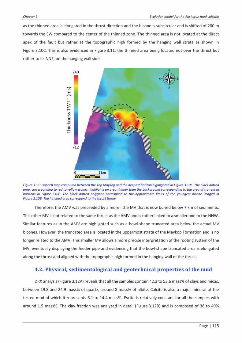
Chapter 3 Evolution model for the Absheron mud volcano
Page | 115
as the thinned area is elongated in the thrust direction and the bicone is subcircular and is shifted of 200 m
towards the SW compared to the center of the thinned zone. The thinned area is not located at the direct
apex of the fault but rather at the topographic high formed by the hanging wall strata as shown in
Figure 3.10C. This is also evidenced in Figure 3.11, the thinned area being located not over the thrust but
rather to its NNE, on the hanging wall side.
Figure 3.11: Isopach map computed between the Top Maykop and the deepest horizon highlighted in Figure 3.10C. The black dotted
area, corresponding to red to yellow wolors, highlights an area thinner than the background corresponding to the area of truncated
horizons in Figure 3.10C. The black dotted polygone correspond to the approximate limits of the youngest bicone imaged in
Figure 3.10B. The hatched area correspond to the thrust throw.
Therefore, the AMV was preceeded by a more little MV that is now buried below 7 km of sediments.
This other MV is not related to the same thrust as the AMV and is rather linked to a smaller one to the NNW.
Similar features as in the AMV are highlighted such as a bowl-shape truncated area below the actual MV
bicones. However, the truncated area is located in the uppermost strata of the Maykop Formation and is no
longer related to the AMV. This smaller MV allows a more precise interpretation of the rooting system of the
MV, eventually displaying the feeder pipe and evidencing that the bowl-shape truncated area is elongated
along the thrust and aligned with the topographic high formed in the hanging wall of the thrust.
4.2. Physical, sedimentological and geotechnical properties of the mud
DRX analysis (Figure 3.12A) reveals that all the samples contain 42.3 to 53.6 mass% of clays and micas,
between 19.8 and 24.9 mass% of quartz, around 8 mass% of albite. Calcite is also a major mineral of the
tested mud of which it represents 6.1 to 14.4 mass%. Pyrite is relatively constant for all the samples with
around 1.5 mass%. The clay fraction was analyzed in detail (Figure 3.12B) and is composed of 38 to 49%

Chapter 3 Evolution model for the Absheron mud volcano
Page | 116
interstratified illite/smectite, 29 to 38% Illite and/or micas and around 15% kaolinite. The rest is composed
of around 5% Chlorite and less than 2% smectite.
Figure 3.12: A, whole rock mineralogical analysis for all the samples collected except the less than 5µm fraction of the MVF1E-RAW
sample, for cuttings from the Anhydritic Surakhany interval and for cuttings from the unstable interval encountered during drilling
operations. The main elements composing the mud are clearly clay minerals and quartz particles and mud samples have similar
mineralogical signature than the unstable interval. B: mineralogical composition of clay for all the samples collected except the
MVF1E-RAW>5µm and for cuttings from Anhydritic Surakhany and the drilled unstable interval. Globally, clay fraction is mainly
composed by up to 50% of interstratified illite/smectite, 30% of Illite and/or micas, 15% of kaolinite and a minor part of chlorite and
smectite, results different from the analysis of the Anhydritic Surakhany and its unstable interval. The less than 5 µm fraction of the
MVF1E-RAW sample differs from the whole samples as they have less illite and/or micas, and more kaolinite and chlorite. See
Figure 3.2 for location map, and Table 2-1 for details of samples.
More details are provided by the results of the two fractions of the same samples (Raw>5µm;
Raw<5µm, see Table 2-1). Even when separating the clay-size particles from the rest, the coarser fraction is
still composed of 31.8 mass% of clay minerals (Figure 3.12) showing the presence of clay aggregates or
claystone clasts larger than 5µm that were not separated during suspension and centrifugation processes
(Figure 3.12). The maximum amount of calcite and the only significant gypsum content are reached on this
fraction with respectively 23.6 and 5.4 mass%. Comparatively with the <5µm fraction, it also contains a
greater part of chlorite with 23% of the clay fraction. Further analysis on the chlorite fraction would be

Chapter 3 Evolution model for the Absheron mud volcano
Page | 117
necessary to conclude on its origin and the reasons for this variability as acid treatment destroys chlorite
minerals.
In the fraction of particles less than 5µm in diameter (Figure 3.12B), there is only 20% illite and/or
micas but also more kaolinite and chlorite (23% and 13% respectively). Illite is known to form at a higher
temperature than interstratified illite/smectite (Pollastro, 1993), which means that the finer fraction is
composed of a smaller portion of high temperature clay minerals than the unseparated samples but is also
composed of more kaolinite and chlorite.
Peaks of carbonates have been observed in the coarser fraction of MVF1E as well as the BC05-DRX5
and the PC12a-DRX4. Sample BC05 was recovered from the top of the mud shield whilst PC12a comes from
the top of the mud flow (Figure 3.2 and Table 2-1. This peak could be the result of the formation of authigenic
carbonate crusts due to methane bubbling through fresh mud after an eruptive phase or at the top of the
structure during a dormant phase (Kopf, 2002; Zitter, 2004).
Thus, the Absheron mud is essentially composed of clay minerals and quartz particles (Figure 3.12).
Clay minerals are not only contained in the matrix as fractions of particles larger than 5 µm also contain more
than 30% of clays.
Biostratigraphic results on pollens and ostracods show a clear difference between samples collected
on the mud volcano or on mudflows and background samples (Figure 3.2 for location). Samples from the
mud volcano shield and the mudflow contain pollens from Miocene to Recent and ostracods from Late
Miocene (Productive Series). Conversely, background sediments when not barren contain pollens from the
Pleistocene and Holocene ostracods (Post-Absheron). Diatoms were only found in shallow background
sediments and mudflows, with Pleistocene to Holocene taxa. The presence of diatoms identical to those of
the background in mudflows and their absence from shield samples may indicate that the flows remobilized
surface sediments on their way downslope and mixed with them. Nannofossil results are not considered
reliable due to the poorness of elements present in the samples. Put together, these biostratigraphic results
seem to indicate that the mud expelled at the Absheron MV only comes from the Productive Series.
Samples for oedometer tests were initially selected based on MVF1 CPT data from the Absheron
mudflow (Figure 3.2 for location, Total proprietary report, Dan & Po, 2017, pers. com.). CPT curves (cone
resistance, pore pressure and friction) present four intervals with distinct evolution of the three measured
parameters. We suppose that these distinct tendencies are related to different intrinsic mechanical behavior
of the mud intervals and oedometer tests were run on one selected reconstituted sample per interval at
water content of around 1.5 wL in order to test this hypothesis (Table 2-1 and Table 3-1). Details on
preparation and results of these oedometer tests are presented in Table 3-1. Oedometer tests presented in
Figure 3.13A show no distinct behavior except for the MECA 10 sample, which also has a slightly different
granulometric curve than the other three selected samples (Figure 3.13C). Indeed, the MECA 10 sample has

Chapter 3 Evolution model for the Absheron mud volcano
Page | 118
a greater fraction of fine material (from 2 to 10 µm) and less coarse fraction (from 30 to 300 µm) than the
three other samples. This also matches with the high initial void ratio and the high compressibility of the
MECA 10 sample with respect to the other samples (Figure 3.13A). Likewise, natural sediments show similar
hydraulic conductivity with void ratio results except for MECA-10 that has a slightly lower permeability trend
in accordance with the lower granulometry of this sample (Figure 3.13B-C).
Figure 3.13: A: oedometer tests with void ratio (e) versus vertical"effective"stress"(#'v)"for"the"different"tested"samples."For"the"natural"
samples, only the MECA-10 has a higher compressibility and a higher initial void ratio than the other samples. The input of coarser
material reduce the initial void ratio and reduce the compressibility of the samples. B: hydraulic conductivity (k) versus void ratio (e)
resulting from oedometer test and falling head method results for the different samples analyzed. Again, MECA-10 has a lower
permeability than other natural samples which fit the same trend. The input of coarser material reduces the hydraulic conductivity
but the general trend stays parallel to natural samples. C: cumulative granulometry for the natural samples showing that MECA 10 is
finer than the three other samples. See Figure 3.2 and Table 2-1 for more details on the samples.

Chapter 3 Evolution model for the Absheron mud volcano
Page | 119
MECA 6-15-22 compressibility curve (Eq. (15)) was considered as representative of all the other natural
mud samples given the very low variability between the three different samples (Figure 3.13A) taken from
different depths of the MVF1 core (Table 2-1).
!" = 4.mp $ b.qr s log"3 (�*(�*+"6" (15)
Permeability results showed no real differences between the different natural samples except for
MECA-10 (Figure 3.13B), and a global linear regression for the other natural samples between ln(K) and the
void ratio was adopted:
ln376 = q.bm! $ tt.pu (16)
Figure 3.13A shows that oedometer tests carried out on natural mud with a coarser fraction are
characterized by a relatively low compressibility with a low initial void ratio (Table 3-1). At around 1000 kPa
of vertical effective stress, the different compressibility curves converge at the same void ratio (Figure 3.13A).
The permeability globally increases with the fraction of coarser material with the same parallel trend as
natural sediments (Figure 3.13B).
4.3. In situ lithology, temperature and excess pore-pressure derived
from in situ well data
The Post-Absheron interval and the Upper part of the Absheron Suite are composed of claystone.
Interstratified claystones and siltstones form the rest of the Absheron Suite and the Akchagyl Suite. The
Anhydritic Surakhany Formation extends from 2501 to 2887 meters TVD/MSL in well B and 2522 to
2905 meters TVD/MSL in well A. It is composed of claystone and evaporitic beds (mainly anhydrite and halite)
and a minor part of siltstone. Over the 400 meters of drilled Anhydritic Surakhany, 30% of evaporitic beds
were encountered with individual thicknesses ranging from less than one meter to eight meters. Finally, the
rest of the Productive Series varies from claystone with rare pluri-decimetric to metric beds of siltstone to
sandstone in the Surakhany (Upper Productive Series) to interstratified claystones, siltstones and sandstones
in the Lower Productive Series. Some of the sandstone beds reach 15 meters in thickness.
Table 3-2 shows the results of NTG calculations based on well B data. The maximum NTG is reached
for the Balakhany-Fasila interval (layer 2 in the numerical model), with a 24% NTG. The Surakhany interval
has only 8% of NTG, and the Novocaspian-Absheron interval has the smallest NTG with 5%. As the well ends
in the NKG interval, the NTG calculation for this particular layer may be inaccurate. From Eq. (3) and (5),
vertical and horizontal hydraulic conductivities were calculated based on sonic logging. The calculated values
fall within the measured ranges of oedometer tests on samples having a coarse content selected on the base
of the NTG value of each interval.

Chapter 3 Evolution model for the Absheron mud volcano
Page | 120
Moreover, an unstable interval was crossed during the drilling of the Anhydritic Surakhany Formation
in well B. This interval, described as a swelling claystone and is interstratified between two 5-meter thick
evaporite layers. A high acoustic velocity and abnormally low electric resistivity characterize the interval.
Cuttings from the interval present a rather similar mineralogical composition to the mud analyzed in this
study (Figure 3.12) with 18.5 mass% of quartz, 34 mass% of clays and micas in which there is 35% illite and/or
micas, 25% kaolinite and no smectite. However, some fractions vary from the mud analyzed: 12.8% of
anhydrite were measured in the unstable interval; none was detected in the mud. Similarly, chlorite is
present at 30% of the total clay fraction when in the mud, less than 10% was measured as well as calcite
which was present at 20 mass% at the considered interval, when around 10 mass% was measured in the
mud.
During drilling, temperatures were also measured at different points of the well allowing to approach
a geothermal gradient of 16 °C/km.
Both wells, which are located 9.5 km west of the mud volcano (Figure 3.14), are overpressured at only
200 to 300 meters below seafloor (BSF) and remain in an overpressured state down to the well bottom.
Overall, shale overpressure increases more or less linearly down to the top Productive Series with a gradient
of 3 MPa/km. Deeper down, the increase is linear again, with a higher gradient. In addition, six pressure
peaks, that are located all along the Productive Series Interval, can be observed in both wells (Figure 3.14).
On these intervals, shale pressure values nearly reach the fracturing pressure, making the concerned intervals
easier to fracture if pressure buildup happens. The concerned formations are the Anhydritic Surakhany (peak
1 in Figure 3.14) as well as five other intervals of the Productive Series.
We noted potential links between structural features and pressure peaks (Figure 3.14). For instance,
the pressure peak 4 in well A, is split into two minor peaks in well B. There is a normal fault cut by well B that
matches the pore pressure decrease observed at well B. Moreover, pressure peaks can be transposed below
the mud volcano to visualize which intervals are more prone to overpressure below the structure.
Pressures were also recorded in the reservoirs. In well A, reservoirs tested above 5000 meters BSF are
in equilibrium with surrounding shales. Below 5000 meters, in wells A and B, reservoirs are at least 20 MPa
below the surrounding shales. In well A, some of these deep reservoirs are as overpressured as the shales.
These results show that shallower reservoirs are not able to dissipate overpressure whereas deeper ones
appear drained and their pressure is much lower than surrounding shales. The deeper reservoir intervals are
known to be regionally continuous and some even outcrop onshore in Azerbaijan (Javanshir et al., 2015).
They act as regional drains for overpressured fluids with a northward hydraulic gradient as shown by the
work of (Bredehoeft et al., 1988; Javanshir et al., 2015). The sands in the northern area of the SCB are at
hydrostatic pressure while an excess hydraulic head creates deeper in the center of the basin.

Chapter 3 Evolution model for the Absheron mud volcano
Page | 121
Figure 3.14: A: overpressure logs for both exploration wells. Overpressures are in MPa. Continuous green line is the sonic-derived shale
pressure and green crosses are the measured reservoir pressures. The orange dots are the LOT/FIT control points used in the
construction of the fracture pressure plot (red line). The vertical line where overpressure is zero is the hydrostatic pressure. Seismic
horizons are shown using the same color code as in Figure 3.3. Six different shale pressure peaks are highlighted in red B: 3D view of
the two parallel seismic lines distant of 9.5 km. The right one is described in Figure 3.4. The left one in Figure 3.3. The pressure peaks
are reported in front of the corresponding interval on seismic.
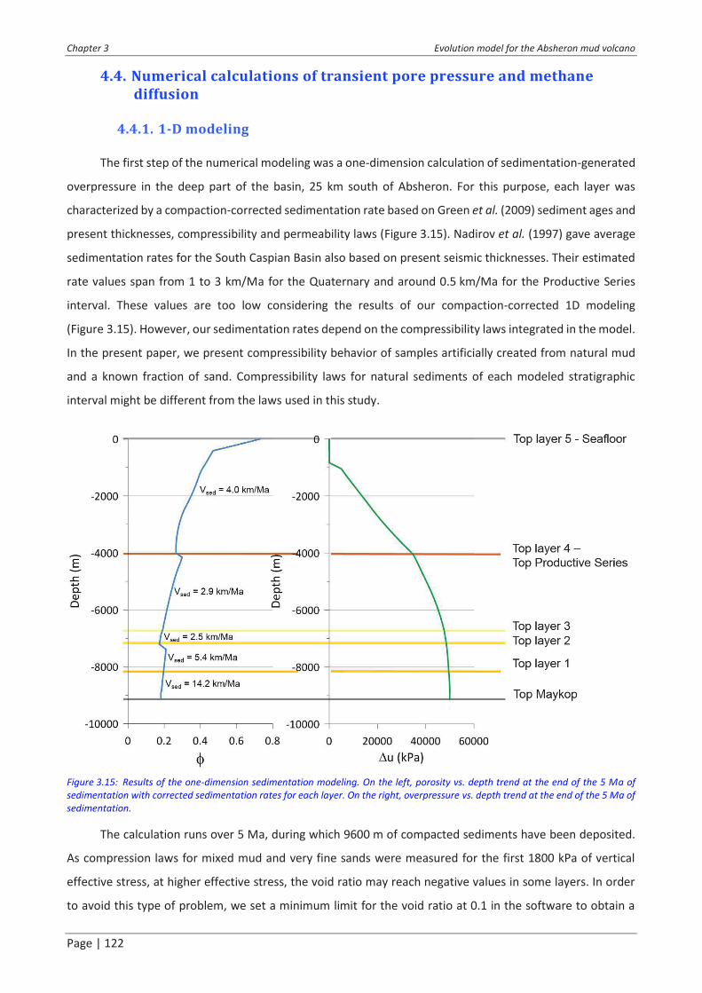
Chapter 3 Evolution model for the Absheron mud volcano
Page | 122
4.4. Numerical calculations of transient pore pressure and methane
diffusion
4.4.1. 1-D modeling
The first step of the numerical modeling was a one-dimension calculation of sedimentation-generated
overpressure in the deep part of the basin, 25 km south of Absheron. For this purpose, each layer was
characterized by a compaction-corrected sedimentation rate based on Green et al. (2009) sediment ages and
present thicknesses, compressibility and permeability laws (Figure 3.15). Nadirov et al. (1997) gave average
sedimentation rates for the South Caspian Basin also based on present seismic thicknesses. Their estimated
rate values span from 1 to 3 km/Ma for the Quaternary and around 0.5 km/Ma for the Productive Series
interval. These values are too low considering the results of our compaction-corrected 1D modeling
(Figure 3.15). However, our sedimentation rates depend on the compressibility laws integrated in the model.
In the present paper, we present compressibility behavior of samples artificially created from natural mud
and a known fraction of sand. Compressibility laws for natural sediments of each modeled stratigraphic
interval might be different from the laws used in this study.
Figure 3.15: Results of the one-dimension sedimentation modeling. On the left, porosity vs. depth trend at the end of the 5 Ma of
sedimentation with corrected sedimentation rates for each layer. On the right, overpressure vs. depth trend at the end of the 5 Ma of
sedimentation.
The calculation runs over 5 Ma, during which 9600 m of compacted sediments have been deposited.
As compression laws for mixed mud and very fine sands were measured for the first 1800 kPa of vertical
effective stress, at higher effective stress, the void ratio may reach negative values in some layers. In order
to avoid this type of problem, we set a minimum limit for the void ratio at 0.1 in the software to obtain a

Chapter 3 Evolution model for the Absheron mud volcano
Page | 123
compressibility trend similar to the ones presented by Chong & Santamarina (2016). Permeability laws for
natural mud and mud mixed with very fine sands obtained from oedometer test results were integrated to
characterize each stratigraphic interval (Figure 3.13A-B). The validity of the permeability laws was confirmed
by the calculations on sonic logging (Table 3-2).
Figure 3.15 shows the porosity profile vs. depth at the end of the sedimentation history. It gives a good
representation of how sediments have compacted during the sedimentation history. The overpressure plot
shown in Figure 3.15 corresponds to the overpressure generated by high sedimentation rates in the deepest
part of the basin. Overpressure rises rapidly with depth in the low permeability layer 5 as overpressure cannot
be evacuated and transmitted rapidly to the whole interval. The increase is slower from Layer 4 down
because of higher permeability. Finally, overpressure increases with a very low gradient from Layer 2 below,
Layer 2 having the highest permeability.
4.4.2. 2-D modeling
The second part of the modeling consisted of creating a structural model for two-dimensional diffusion
of overpressure and methane. The structural model presented in Figure 3.16 is based on the work of Green
et al. (2009) and on the fault network observed on the reference section in Figure 3.3. The initial section
presented by Green et al. (2009) was only reproduced from the deeper part of the basin to the Absheron
Ridge, where the seafloor is shallowest. The direction is the same as the section presented in Figure 3.1B.
The total length of the section is 55 km, and its maximum depth 9.6 km. Faults shown in Figure 3.16 are
meant to represent not only the fault surfaces (localized thin shear zone), but also to the damage zone
surrounding them. We estimated the thickness of the damage zone based on the work of Savage &
Brodsky (2011), who relate the damaged thickness around a fault to the throw of the fault. With a total throw
about 1 sec TWTT for the main, a damage zone of a few hundred meters is expected. In the present work, a
damage zone of 300 meters is considered as representative of the fault zones.
Figure 3.16 shows the boundary conditions used for the numerical calculation of methane and pore
pressure diffusions. No lateral or vertical exchange of pore pressure and methane with the outside of the
model is permitted through the laterally impermeable southern and northern borders and the vertically
impermeable upper and lower borders. The sea water has a fixed pore pressure of 0 kPa and a methane
concentration of 1.0 x 10 � 5 mM (milli-molar, 1 molar corresponding to a solution of 1 mol/L of concentration)
which is a mean oceanic value (Lamontagne et al., 1973). The pore pressure calculated in one dimension from
sedimentation with SeCoV3 (Figure 3.15), is imposed at the southern border of the model, where the
sedimentary column is the thickest. Finally, a methane concentration of 1.0 x 10 � 3 mM is fixed at the bottom
of the fault network, methane being generated in the Maykop Formation, the regional source rock, the
deeper layer represented in the model.

Chapter 3 Evolution model for the Absheron mud volcano
Page | 124
Figure 3.16: Structural model based on Green et al. (2009) work and on the fault network observed in Figure 3.3. The line follows the
same trend as the seismic section of Figure 3.1B. Eight layers extend along the section corresponding to different sedimentation rates,
compaction laws and permeability trends (see Figure 3.15). The Layers NKG, Balakhany-Fasila, Sabunchy, Surakhany and Quaternary
are named Layers 1 to 5 respectively in other figures. Numbers showed at the limits of the model correspond to limit conditions
imposed for the diffusion of pore pressure and methane.
Pressure and methane migration calculation were run over 5 Ma. Results of the diffusion equation
resolution (Eq. (9) and (10), Chapter 2:3.4.2), in terms of overpressure migration, are shown in Figure 3.17A.
Methane concentration and ratio between overpressure and vertical effective stress are shown together in
Figure 3.17B in order to compare possible hydrofractured zones with high dissolved methane saturated
areas.
Overpressure (Du) propagated from south to north of the model at different diffusion rates. Indeed,
depending mainly on permeability laws, overpressure will propagate more or less quickly and in different
directions. For instance, in layer 5 overpressure did not accumulate (Figure 3.17A). This layer being the
youngest, it maintained a high void ratio and so a higher permeability. The effect is amplified by the ratio
between horizontal and vertical permeabilities. Layer 5 having a ratio of 2200 (Table 3-2), the horizontal
permeability in the model is 2200 times larger than the permeability defined by oedometer test results.
Therefore, in layer 5, pressure diffusion is mainly horizontal and the seawater condition (no overpressure)
has significant impact on the overpressure values of this interval. From layer 4 below, the pressure is mainly
diffused laterally creating a pressure front. At a given distance from the south of the model, where
overpressure was injected from one-dimension sedimentation modeling (Figure 3.16), overpressure is larger
in layer 4 than in other layers reproducing the pressure peaks observed at the wells (Figure 3.14).

Chapter 3 Evolution model for the Absheron mud volcano
Page | 125
Figure 3.17: Results of overpressure and methane migration modeling after 5 Ma of calculation. A: overpressure (Du) in kPa after 5 Ma of migration through the structural model presented on Figure 3.16.
Overpressure migrated more rapidly through layer 4 which has a higher permeability. B: Du/s�v contours with values exceeding 0.75 and potentially reaching the level of hydro-fracturing. High values
located in layer 5 are due to the low s�v near the seafloor. Black lines correspond to methane concentration contours. The top of the methane-saturated area corresponds to a zone where hydro-fracturing
may occur if overpressure was slightly higher. Black dotted lines are for layer limits.

Chapter 3 Evolution model for the Absheron mud volcano
Page | 126
Faults and associated damage zones were designed to rapidly diffuse methane therefore artificially
reproducing methane advection through fractured zones. Methane was injected at the base of the fault
network with a concentration of 1.0 x 10 � 3 mM (Figure 3.16). Methane molecular diffusivity in the rest of
the model is three orders of magnitude lower than in faults. As a result, methane rapidly saturated the area
adjoining the faults, and then diffused slowly through the sedimentary column until saturating an area nearly
2 km wide around the fault network (Figure 3.17B). The ratio of overpressure over vertical effective stress
(Du /s�v) is higher in layer 5, particularly in the north of the model. As it is the shallowest interval, s�v is the
lowest of the model. Besides, little overpressure accumulation was possible in layer 5. Nevertheless, values
are high at the top of the layer 4, where the ratio varies between 0.5 and 0.6. So we expect critical values in
the area of high methane saturation at the Absheron crest.
5. Discussion
5.1. What is the stratigraphic source of the mud?
The geomorphological description of the Absheron mud volcano evidenced a bowl-shaped geometry
below the mass extruded through the Absheron interval (Figure 3.5). This feature is formed by the Anhydritic
Surakhany horizons that terminate as truncations (Catuneanu et al., 2009) below the younger seismic
horizons of the Upper Productive Series. Truncations are also observed 500 m below, in the lower part of the
Upper Productive Series. Horizon continuity resumes in the Middle Productive Series. This particular
geometry was already described and corresponds to a depleted area forming a potential former mud
generation zone (Stewart & Davies, 2006; Dupuis, 2017; Kirkham et al., 2017b; Dupuis et al., 2019). The
presence of two truncated intervals (Figure 3.5) indicates that there may have been several mud generation
stages.
The unstable interval drilled in the Anhydritic Surakhany has a mineralogical composition similar to the
mud analyzed in this study (Figure 3.12), with nearly 50% of clay minerals. Mud sampled at the seafloor is
poorer in Anhydrite, chlorite and calcite than the unstable interval analyzed in the Anhydritic Surakhany
Formation. The mineralogical differences may be explained by the different paths and histories of the
samples. Mud was driven upwards and deposited at the seafloor after a catastrophic event leading to
remobilization of deep sediments. Thus, it potentially interacted with seawater but also with deeper fluids
and gases forming for instance carbonate crusts at some methane seeping points or during diffuse degassing
after a mud eruption (Kopf, 2002; Zitter, 2004). Conversely, the unstable interval cuttings were extracted
directly from the formation through the drilling process and was in contact with the drilling mud.
From the biostratigraphic analysis of the mud and recent background sediments deposited at the
seafloor, we can infer a Late Miocene to Pliocene (Productive series) origin for the mud.

Chapter 3 Evolution model for the Absheron mud volcano
Page | 127
Mineralogical analysis showed that fine fraction is poorer in illite and micas than unseparated samples
(Figure 3.12B). These minerals are high temperature minerals compared to smectite or interstratified
illite/smectite (Pollastro, 1993). Unseparated samples are composed of a non-negligible fraction of diverse
clasts when the fine fraction extraction is constituted of mud matrix particles. Therefore, clasts and coarse
particles may find their source deeper than the mud matrix. However, the presence of a larger percentage
of chlorite in the fine fraction (Figure 3.12B) tends to show a degradation of micas and illite in the mud matrix.
The contact of deep fluids and seawater with the mud matrix particles may be responsible for this reaction
while coarser particles and clasts may preserve better illite and micas. Thus, mineral reactions with deep
fluids and seawater could explain the different mineralogical compositions of mud matrix and they might
come from the same depth magnitudes.
The Anhydritic Surakhany interval has several particularities. First, it is composed of 30% of evaporitic
beds that can reach up to 8 meters in thickness. The rest is mainly composed of claystones. An
unstable interval was noticed during drilling but others may exist in the Anhydritic Surakhany. Therefore, this
interval may have a specific mechanical behavior. Moreover, the thermal gradient approximated from the
temperatures measured at the wells is 16 °C/km which is in accordance with mean thermal gradients
measured at other SCB locations (Ginsburg et al., 1992). Considering that the mud volcano activated after
deposition of H3 (Figure 3.5), and considering that the thermal gradient remained constant during the
Quaternary, the Anhydritic Surakhany temperature was around 30°C when the first eruption occurred. Day-
Stirrat et al. (2010) state that above 80°C, chemical compaction (cementation processes, precipitations) will
strengthen the mudstone fabric and this process is irreversible i.e. the mudstone can no longer behave in a
ductile way. Thus, the Anhydritic Surakhany Formation would have been well within the temperature range
where ductile deformation is conceivable.
Finally, overpressure logs show that the Anhydritic Surakhany forms a pressure peak at both wells
(Figure 3.14). Rupture in this interval would happen earlier than in other formations for a given pressure
increase or stress decrease. The fact that highly overpressured mudstones are blocked between meter-thick
layers of evaporites may explain the weak behavior of some layers. As compaction water cannot be expelled
vertically because of evaporites, these layers are likely to stay under-compacted and overpressured.
From these observations and measurements it seems plausible to conclude that Upper Productive
Series, and more precisely the Anhydritic Surakhany Formation, is the source of the solid fraction of the mud
expelled at the Absheron mud volcano.

Chapter 3 Evolution model for the Absheron mud volcano
Page | 128
5.2. How do the field pore pressure measurements compare to the
model?
It is quite clear on pressure logs that pressure regimes are completely different in shales and in
reservoirs. Indeed, shales are highly overpressured all along the well, following a trend nearly parallel to the
lithostatic pressure from the Top Akchagyl to the Bottom Productive Series. In the bottom part of the wells
(from the PS2 seismic horizon downwards), overpressure level in shales remains rather constant while
reservoir pressures are nearly hydrostatic. Javanshir et al. (2015) describe similar pressure regime and
magnitudes in the neighboring Shah Deniz fold. The Upper Productive Series there have equal sandstone and
shale overpressures and as the reservoir facies become more abundant and continuous in the Bottom
Productive Series, they become less overpressured. Therefore, in Shah Deniz and Absheron, the deep
reservoirs seems to act as permeable drains as they allow overpressure to dissipate. The fact that shale
pressure is also affected shows that dewatering might occur in the thinner shale intervals contained in the
Bottom Productive Series. Indeed, the abundance of permeable reservoirs would allow compaction water to
be drained away from the shales, reducing their pressure. There is lateral pressure transmission from the
deep part of the basin to the edges through regional-scale reservoirs (Javanshir et al., 2015), from the south
to the north of the sections presented in Figure 3.14.
However, pressure horns in Absheron shales are not recorded in the data of Javanshir et al. (2015).
Some intervals of the Productive Series of Absheron wells are more overpressured than the rest of the
stratigraphic interval. These peaks bring the corresponding intervals to pressure values between 5 and 10
MPa below hydrofracturing pressure in wells located 9.5 km from the mud volcano center. The difference
between hydrofracturing pressure and shale pressure may be even smaller near the mud volcano, or it may
have been smaller in the past, before mud volcano activation. Therefore, they represent weak areas where
a local rise in overpressure through clay dehydration or tectonic overpressuring for instance (Osborne &
Swarbrick, 1997), or a drop in effective stress (erosion or fold growth and crestal uplift) could generate
hydrofractures.
Pressures recorded in the two wells are not exactly the same (Figure 3.14): in the southern well
(Well A), shale pressure decrease more gently within the Bottom Productive Series and reservoir pressures
are higher. Moreover, pressure horns are stronger in well B (to the north). Differential sedimentation
between the deep basin located at the south of the Absheron anticline and the northern edge of the basin
where less sediments accumulate could explain this phenomenon (Grosjean et al., 2009; Javanshir et
al., 2015). As pressure transmission is oriented roughly from the south to the north of the anticline, the
northern side of the anticline would accumulate more overpressure in the shales whereas reservoirs would
be more drained than in the southern flank. This phenomenon was also noted at the neighboring Shah Deniz
anticline (Javanshir et al., 2015).

Chapter 3 Evolution model for the Absheron mud volcano
Page | 129
2D model sections reproducing the main features of the pressure plots are shown on Figure 3.17. The
overpressure rises down to 2000 and 5000 meters deep depending on the location. Then overpressure
remains constant at 30 MPa at the Absheron location and even decreases to 25 MPa when reaching the
bottom part of the Productive Series where highly continuous and abundant reservoir facies are present.
Moreover, the numerical modeling results emulate the Top Surakhany pressure horn. Yet, the modeling
results underestimate the overpressure at the Absheron location (Figure 3.17A) as they are not in accordance
with overpressure values recorded at the wells. Indeed, from Top Surakhany down, overpressure reaches
values between 20 MPa and 50 MPa. The discrepancy between measured and calculated overpressures may
be related to the compressibility and permeability laws applied to the model which were obtained from
artificial (reconstituted) sandy-clayey samples and not from natural samples from the different stratigraphic
layers. Besides, the considered source of overpressure is related to fast sedimentation and might not be
sufficient to model the natural pressure conditions of the Absheron anticline. Indeed, additional sources of
pore pressure may play an important role and are yet to be considered in the modeling work.
However, and as a first approach, the present calculation was able to reproduce the main overpressure
trends visible at the wells.
5.3. How does methane diffusion interact with excess pore pressure
accumulation?
From results of the pressure generated by potential gas columns that could have been trapped in the
ASF at the time of the AMV activation, it is clear that external parameters are needed in order to explain the
AMV formation. The effect of high sedimentation rates and basin wide lateral pressure transmission on the
overpressure at the Absheron location was therefore studied through numerical modeling. The significant
lateral fluid migrations through the SCB was already shown by Bredehoeft et al. (1988), Javanshir et al. (2015)
and Gautherot et al. (2015).
Modeling results shows that high values of Du /s�v fit with high dissolved methane concentrations and
occur around the fault network below the Absheron mud volcano (Figure 3.17B). The consequence of high
Du /s�v causing hydrofracturing may be an important decrease in pore pressure leading to methane
exsolution and expansion (Duan & Mao, 2006) and generation of overpressured mud. Gas exsolution in
sediments has proved to be a critical factor controlling sediment damage. Indeed, experience on gassy
sediment core recovery in deep water shows important damage and loss of structure during the core ascent
to the surface and associated hydrostatic pore reduction (Sultan et al., 2012). Loss of acoustic signal
corresponding to the presence of free gas correlates with dramatic decrease of the yield stress ratio
illustrating the damage made to the sediments.
Moreover, the presence of normal faults at the anticline crest between the Upper Productive Series
and the Top Absheron (Figure 3.3) shows that the state of stress where the primary source of mud was

Chapter 3 Evolution model for the Absheron mud volcano
Page | 130
identified was extensive at the time when the Absheron mud volcano formed. If compressive state was
dominating at these time and location, the observed faults must have been thrusts. Therefore, s1 (the
maximum principal stress) was certainely vertical, so the least principal stress was horizontal. Fractures opens
in the direction of the least principal stress and then propagates in a plane perpendicular to this direction
(Hubbert & Willis, 1957). Thus, hydrofractures generated at the time of the mud volcano formation above
the mud generation zone are expected to be vertical.
A present-day studied example of clastic extrusion triggering displays similar results. Indeed, the Lusi
disaster, whose 2006 triggering cause is still a matter of debate between an earthquake and drilling issues
(Mazzini et al., 2007; Tingay et al., 2008, 2017), was initiated by the combination of under-compaction /
overpressure in the source layer and the presence of dissolved and free gas. According to Davies et al., (2008),
fractures generated by drilling activities have caused an important decrease in pore pressure and the
consequence was gas exsolution and expansion, overpressured mud generation and the extrusion of mud to
the surface (Davies et al., 2008). However, Mazzini et al. (2012) proposed an hydrothermal source for the
gas, yet Lusi triggering is already explained by gas flowing in under-compacted and overpressured sediments.
Thus, we suggest that the theoretical mechanism we propose for mud generation and extrusion with
a combination potential fracture zones and gas-saturated areas would also be applicable to the Absheron
fold, where the studied mud volcano is located.
5.4. What is the most plausible sequence for the formation of the
Absheron mud volcano
Based on previous observations and conclusions, a qualitative formation model for the Absheron mud
volcano is proposed. This model is developed in six main phases:
Phase 1: rapid deposition of the Productive Series (over 3.5 km in 2 Ma) above the gas-mature Maykop
Formation that would generate hydrocarbons migrating slowly through the sedimentary column
(Figure 3.18-1). Maykop Formation started generating gas during the Late Miocene in the Shah Deniz region
located less than 50 km from Absheron gas discovery (Figure 2.9 in Alizadeh et al., 2017). Moreover, the
deposition of the Anhydritic Surakhany Formation proves that the sea level must have been lower than
nowadays at the end of the Productive Series deposition.
Phase 2: folding started during deposition of the Akchagyl Suite. It is linked to the propagation of a
deep thrust terminating in the Maykop formation and linked to normal faults related to the fold formation.
Methane migration is then focused into the faulted core of the anticline (Figure 3.18-2). The folding also has
the effect of generating preferential rupture zones at its crest (Figure 3.18-2). Indeed, at the anticline crest,
s�v is lower than on the flanks. Besides, as more space is available for sediment deposition in the surrounding
synclines and in the deeper part of the basin, overpressure is generated and transmitted towards the

Chapter 3 Evolution model for the Absheron mud volcano
Page | 131
Absheron location. Overpressure generation and transmission as well as lower s�v at the crest increases the
Du /s�v ratio thereby increasing pore gas solubility.
Phase 3: Du /s�v ratio reaches the hydro-fracturing threshold (Figure 3.18-3), leading to a significant
decrease in pore pressure.
Phase 4: hydrofracturing triggers gas exsolution and expansion in gas-saturated and mechanically weak
layers such as Anhydritic Surakhany Formation (Figure 3.18-4). Exsolution remobilizes the weak interval,
generating mud. Overpressured and low-density mud is then transported to the seafloor provoking the first
mud extrusion. As gas, mixed with sediments and water, migrates up the hydrofracture network, methane
expands amplifying the process and potentially eroding fracture walls (Figure 3.18-4).
Phase 5: the process goes on with gas exsolution propagating in the Anhydritic Surakhany, depleting
this layer continuously. Collapse of the upper strata into the depleted area creates the rather flat and low
topography volcano (Figure 3.18-5). The extruded mud slowly degasses at the seafloor.
Phase 6: quiescent and active phases of the mud volcano alternates, creating a complex interdigitation
geometry where normal sedimentation predominates during quiescent phases of the volcano. Further
depletion happens in the source, triggering more collapse, while more mud is extruded at the seafloor
(Figure 3.18-6).
The initial trigger of this mud volcano is not related to gas, as hydrofracturing due to overpressure
build-up and weakness of the fold-crest initiates the succession of events. However, in this conceptual model,
methane would have three essential effects:
· Gas needs to saturate the porous network in its dissolved state before hydrofracturing in order
to provoke remobilization of sediments. Exsolution of methane weakens and disaggregates
host sediments (Sultan et al., 2012; Tingay et al., 2015).
· As free gas has very low density (typically about 1/1000 of that of water in normal conditions),
it will flow towards the surface (Brown, 1990), carrying the mud away (solid particles and
formation water).
· Finally, as gas goes up into the pipe, it expands (Brown, 1990), accelerating the mud ascent,
sustaining mud pressure and eroding fracture walls, creating clasts, to end-up with mud
breccia extrusion at the surface.

Chapter 3 Evolution model for the Absheron mud volcano
Page | 132
Figure 3.18: Formation model for the Absheron mud volcano based on in situ observations and measurements, laboratory tests and analysis and numerical modeling. 1- Rapid deposition of the Productive
Series and maturation of the Maykop formation. Slow and extended methane migration. 2- Absheron fold creation. Focusing of the methane migration through fold-related fault network and Du/s�v
increase at the anticline crest. 3- Rupture condition reached and hydrofracturing of the sedimentary column from the seafloor to the Anhydritic Surakhany. 4- Gas exsolution and expansion and
remobilization of Anhydritic Surakhany sediments. First extrusion. 5- Propagation of gas exsolution and sediment remobilization. Depletion of the Anhydritic Surakhany and collapse of the overlying
strata. 6- present geometry after alternation of several quiescent and active episodes for the mud volcano. More depletion of the source and collapse of the overlying strata is triggered at each active
episodes.

Chapter 3 Evolution model for the Absheron mud volcano
Page | 133
Thus, methane exsolution is the key to mud formation but also the main driver for mud remobilization
towards the surface due to its low density and expansion capacity. Initial rupture is essential in order to start
the chain reaction and methane expansion and exsolution will maintain the pipes open and even enlarge
them.
5.5. Limits and perspectives of the study
This conceptual formation model of the AMV closely fits with observations and analysis of the available
dataset and is partly based on the numerical modeling results presented earlier.
However, improvements may be made at several levels:
Dataset: For instance, the seismic masking prevents direct observation of the center of the volcano�s
plumbing system. Re-processing of the data was attempted several times and with different methods and
approaches, but it remains challenging due to the presence of gas-charged mud and free gas. The available
biostratigraphic analyses are not quantitative and for further precision on the mud origin quantitative
analyses of the fauna and flora in mud will be necessary. Analysis of the clasts will also help to refine the mud
origin.
Numerical modeling: The compressibility laws used in the current model could be improved to
consider soil compressibility for the highest stress range (Chong & Santamarina, 2016). In the present work
and in order to avoid negative void ratio values, the software limits the minimum void ratio to 0.1. In the
present model, pore pressures generated by sedimentation and pressure transmission are not calculated
simultaneously. Overpressure due to sedimentation is calculated over 5 Ma of sedimentation history and is
integrated as a boundary condition into the 2D Darcy�s and Fick�s diffusion equations. The next step would
be to integrate both sedimentation and diffusion processes into one unique 2D model. Finally, the model
does not simulate the post-hydrofracturing process causing gas exsolution and overpressured mud expulsion.
Gas exsolution and expansion processes will have to be integrated into this model in order to reproduce mud
volcano initiation.
Overpressure generation mechanisms: the mud volcano is located at the crest of an active anticline
and triggered after one of the main folding phases. Thus lateral tectonic overpressuring is expected to have
happened before the mud volcano formation (Osborne & Swarbrick, 1997; Swarbrick et al., 2002). This
tectonic overpressuring has prooved to increase the global ovepressure up to 16 MPa at 3.5 km deep partly
due to porosity decrease (Couzens-Schultz & Azbel, 2014; Obradors-Prats et al., 2017). Moreover, internal
sources have not been considered such as clay dehydration and smectite-illite reactions that generate a large
volume of water in the pore space, thus generating overpressure (Osborne & Swarbrick, 1997; Swarbrick et
al., 2002). Gas generation is also considered as an overpressure generation mechanism and may have
implications for this numerical model as gas is generated and diffused through the sedimentary column

Chapter 3 Evolution model for the Absheron mud volcano
Page | 134
(Osborne & Swarbrick, 1997; Swarbrick et al., 2002). Considering these new pore pressure input, the Du /s�v
ratio may increase drastically and the model may be able to reproduce the observed in situ pore pressure
measurements.
Moreover, the presence of the buried MV gives the possibility to enrich our model of MV formation
with other important elements. When comparing the AMV with the small MV, several common
characteristics appear. Both MVs are directly related to deep thrusts and the setting of anticline crests (the
hanging wall topographic high in the case of the small MV, Figure 3.4 and Figure 3.10C). Similar architectural
elements were observed such as a bowl-shaped depleted area corresponding to the mud generation zone
(Figure 3.5 and Figure 3.10C). The small MV brings further details on what could be the precise 3D
architecture of the AMV rooting system. The depleted area of the small MV is elongated along the thrust
direction and thus, it is not a perfect bowl-shaped area (Figure 3.11). Moreover, centered into the collapsed
strata, what could be the feeding pipe is imaged. The extruded structures and the depletion zone are not
perfecty aligned and have not the same shape (Figure 3.11). Therefore, the AMV may present similar features
that are masked by the imaging issues due to gas and the presence of low-velocity mud.
However, despite the similarities, both structures are different. First, the timing of formation is not the
same. The small MV is much older than the AMV as its extruded structures are now buried 7 km below
seafloor. The presence of the small MV above the northern thrust confirms that the northern thrust is older
than the thrust coring the Absheron fold. Moreover, the mud generation zones are not in the same
stratigtraphic intervals. The AMV is related to the ASF while the small MV is related to the Maykop Formation.
This shows, as highlighted by other authors (Yusifov & Rabinowitz, 2004; Dupuis, 2017), that all MVs in the
SCB may be different and are not all related to the Maykop Formation, even in the same area. Besides, the
small MV was formed before the Maykop Fm becomes mature to gas. Therefore, all these differences could
relate to different formation mechanisms.
This comparision shows the possibility to compare MV structures to better understand their
morphology but also the necessity to study each structure separately when dealing with formation processes,
each MV being related to specific conditions.
6. Conclusions
Based on 3D seismic data, mineralogical, geotechnical and biostratigraphic analyses of the sampled
mud together with well data, we conclude that the Anhydritic Surakhany Formation is a plausible source for
the Absheron mud volcano. Pressures recorded at the wells show, as in Shah Deniz, that deep reservoirs act
as drains for pressure provoking a decrease in overall shale pressure logs. Pressure horns were also recorded
at specific intervals, as for the ASF, where shale pressure is close to the fracture limit.
Chapter 3 Evolution model for the Absheron mud volcano
Page | 135
Based on these observations, a numerical model with 2D-diffusion equations was applied on a basin
scale section. Sedimentation-related overpressures underestimate by 50% the pressures measured in the
wells but reproduce fairly well the observed trends. Additional sources of in situ overpressure generation
(i.e. clay dehydration and transformation), which are not included in the current model, may explain the
discrepancy between the model prediction and the pore-pressure values of wells. The main observation
made through the numerical model is the superposition of methane-saturated areas with potential
hydrofracturation zones. Indeed, hydrofracturing may produce a drastic decrease in pore pressure, allowing
gas exsolution and expansion. Based on the present model results, on experimental results of gassy-sediment
behavior in which the gas exsolution damages the sediment and reduces its mechanical strength and on the
Lusi disaster studies, we conclude that the superposition of potential hydrofracturing areas and gas-saturated
zones can explain that the Absheron mud volcano activated at the crest of the anticline.
As a result, we propose a conceptual evolutionary model for the Absheron mud volcano as follows:
initial stages of folding focus methane migration into the anticline crest bringing methane to the upper
geological layers and mainly to the Anhydritic Surakhany Formation. Pore pressure accumulation and its
lateral migration through the Anhydritic Surakhany Fm. promote hydrofracturing at the location of the
Absheron mud volcano causing a decrease in pore pressure. These conditions lead to methane exsolution
and expansion and to the upward remobilization of the already weak Anhydritic Surakhany interval,
generating low density and overpressured mud. During mud ascent, gas bubbles expand, splintering fracture
walls and incorporating clasts into the mud. Finally, extrusion at the seafloor happens where the mud slowly
expels methane. As extrusion continues, a collapse of the overlying strata into the depleted mud generation
zone forms.
Therefore, even though the trigger point for the whole MV formation process in our model is
hydrofracturing, clay-rich sediments have to be initially saturated with methane in order to generate mud.
The methane is essential and has three main roles: exsolution allows creating mud from weak layers, its low
density decreases that of the mud and accelerates its upward flow to the surface, and gas expansion
decreases mud density, which causes splintering of gas-saturated fracture walls creating clasts.
With the available dense dataset, we highlight that, in order to form the Absheron mud volcano, a
combination of three factors is required: high pore pressure, gas saturation and clay-rich sediments. Recent
work on the Lusi eruption also demonstrated the importance of the same factors in a different geological
environment. Therefore, detecting the presence of these three factors may help understand the
preconditioning factors of MV formation.

Chapter 3 Evolution model for the Absheron mud volcano
Page | 136

Page | 137
Chapter 4: Sediment damage caused by gas exsolution: a key mechanism for mud volcano formation
Abstract
Gassy sediments are common in marine environments and are characterized by a specific mechanical
behavior significantly different from that of water-saturated sediments. It is shown that gas causes damage
and initiates fractures in sediments. To define the controlling parameters dominating the damage process
during gas exsolution and its consequences in terms of hydro-mechanical behavior, we developed a specific
consolidation apparatus to test sediments from the active Absheron mud volcano (South Caspian Basin).
Indeed, mud volcano formation is initiated by gas exsolution and expansion and subsequent mud formation
as demonstrated in Chapter 3.
Gas was generated in the studied samples by circulating carbonated water through the sediment and
then decreasing the total pressure. Particular attention was given to the impact of gas saturation and
associated damage and fractures on P-wave velocity, sediment compressibility, permeability and
preconsolidation pressure. Results show that fracture geometry is mainly controlled by the degree of gas
saturation and preconsolidation pressure. The damage level increases with the degree of gas saturation while
the elastic modulus of sediments is degraded. Experimental data show that sediments do not entirely recover
their original mechanical behavior when gas disappears. Finally, the experimental data confirm that gas
exsolution and expansion in the host sediment can lead to mud formation.

Page | 138

Page | 139
Chapitre 4 : Endommagement des sédiments par exsolution de gaz : un mécanisme clé pour la formation des volcans de boue
Résumé
Les sédiments gazeux sont fréquents dans les environnements marins et ils sont caractérisés par un
comportement mécanique qui diffère de celui d�un sédiment saturé en eau. La présence de gaz dans les
sédiments marins est un facteur d�endommagement et de fracturation. Afin de définir les paramètres qui
contrôlent l�endommagement des sédiments lors de l�exsolution de gaz ainsi que les conséquences causées
sur leur comportement hydromécanique, une cellule de consolidation spéciale a été développée afin de
tester des sédiments prélevés sur le volcan de boue actif d�Absheron (Bassin sud caspien). En effet, la
formation d�un volcan de boue est initiée par l�exsolution et l�expansion du gaz dans les sédiments, générant
la boue en profondeur comme montré dans le Chapitre 3.
Du gaz a été libéré dans les échantillons sédimentaires en y faisant d�abord circuler sous pression de
l�eau saturée en dioxyde de carbone, puis en faisant chuter la pression totale à la suite de la consolidation.
Les effets de la saturation en gaz et ses conséquences sur l�endommagement et la fracturation ont été
observés en mesurant et en analysant la vitesse des ondes P, la compressibilité du sédiment, sa perméabilité
et sa pression de préconsolidation. Les résultats montrent que la géométrie des fractures est principalement
contrôlée par le degré de saturation en gaz et la pression de préconsolidation. Le niveau d�endommagement
augmente avec le degré de saturation en gaz, et en parallèle, le module élastique du sédiment est dégradé.
Les résultats expérimentaux montrent que le sédiment ne recouvre pas complétement son comportement
mécanique initial lorsque le gaz disparait. Enfin, les essais confirment que l�exsolution et l�expansion du gaz
dans les sédiments peuvent mener à la formation de boue.

Page | 140

Chapter 4 Sediment damage caused by gas exsolution
Page | 141
1. Introduction
Sediments partially saturated with free gas are a widespread occurrence and are found in varying
marine environments (Grozic et al., 2000). Nageswaran (1983) discriminates between two free-gas
distributions: continuous gas phase and discrete separated gas bubbles. The latter is defined as gassy
sediments and Nageswaran (1983) gives a maximum limit in terms of the degree of gas saturation (Sg < 15%).
Gassy sediments are a well-known issue in marine geotechnics that have been studied for decades as the
detection and quantification of free-gas content is essential for geohazard assessment (Esrig & Kirby, 1977;
Sobkowicz & Morgenstern, 1984; Thomas, 1987; Sultan et al., 2004, 2012; Judd & Hovland, 2007; Riboulot et
al., 2013).
The main difficulty when studying gassy sediments in the laboratory is to obtain a discrete distribution
of gas bubbles. Several techniques exist including the generation of free gas through the zeolite molecular
sieve technique (Nageswaran, 1983; Thomas, 1987; Wheeler, 1988; Sills et al., 1991; Nava Castro et al., 2013),
the generation of biogenic gas through bacteria (Sills & Gonzalez, 2001; Rebata-Landa et al., 2012) and finally
the generation of gas bubbles through the circulation of overpressured carbonated water followed by
decompression (Grozic et al., 2000; Sultan et al., 2012). Each method is detailed in Chapter 4:2.3.
The mechanical behavior of gassy sediments has been extensively studied over the last few decades
and all the studies demonstrate that it differs completely from saturated sediment behavior (Thomas, 1987;
Wheeler, 1988; Sills et al., 1991; Helgerud et al., 1999; Grozic et al., 2005; Sultan et al., 2012; Nava Castro et
al., 2013; Jang & Santamarina, 2014). Details on the hydro-mechanical properties of gassy sediments are
provided in Chapter 4:2.4.
Mud volcanoes are one of the most spectacular geological features related to gas venting. Gas, mostly
methane and carbon dioxide, is expelled at the seafloor along with a fluid melange, varying in proportion, of
water, fine-grained sediments and larger rock fragments (Kopf, 2002; Mazzini & Etiope, 2017). Mud is
commonly sourced from depths of several kilometers (Stewart & Davies, 2006; Kirkham, 2015; Blouin et
al., 2019). The Lusi catastrophe, ongoing since 2006, allowed to monitor mud volcano generation from its
initiation (Tingay et al., 2008, 2017; Mazzini et al., 2012). Tingay et al. (2017) demonstrated that the key
parameters of the Lusi triggering were the high overpressure and the gas influx into weak layers. Moreover,
Capaccioni et al. (2017) show that the emplacement of sand volcanoes during Cone Penetration Testing in
Italy was caused by gas exsolution and expansion in loose deposits. Therefore, Tingay et al. (2015) and Blouin
et al. (2019) proposed gas exsolution and expansion triggered by hydrofracturing and the subsequent drop
in pore fluid pressure as mud generation mechanisms.
The aim of this present study is to identify the impact of gas expansion and exsolution on the
mechanical behavior of sediment sampled directly from an active mud volcano (Absheron mud volcano AMV,
Chapter 4 Sediment damage caused by gas exsolution
Page | 142
South Caspian Basin; Blouin et al., 2019). Particular attention was given to the gas impact on sediment
structure, acoustic properties (P-wave velocity), compressibility and preconsolidation pressure by carrying
out a series of consolidation/compressibility tests using a novel experimental set-up. The main questions
motivating this work are summarized below:
· If gas exsolution within sediment is already proven to cause damage (Sultan et al., 2012), what
are the controlling parameters dominating the process and what are the consequences in
terms of hydro-mechanical behavior?
· Do the mechanical properties of the sediment recover from gas exsolution/expansion after
mechanical reloading?
· What are the conditions that allow gas exsolution and expansion in the host sediment to
generate mud?
2. State of the art on gassy sediments
2.1. Definition of gassy sediments
Natural soils are not always saturated with water; instead, their voids can be filled partly with water
and with free gas/air and the soil are therefore called unsaturated soils (Nageswaran, 1983; Wheeler, 1986;
Thomas, 1987). Depending on the degree of gas saturation (Sg), the structure of unsaturated soils may vary
greatly (Wheeler, 1986). Figure 4.1 shows three possible structures for unsaturated soils depending on the
Sg. For high Sg, the water phase will be discontinuous and occluded between grain contacts and the gaseous
phase is continuous (Figure 4.1a; Wheeler (1986)). For intermediate Sg, the two phases are continuous
(Figure 4.1b; Wheeler (1986)). For small Sg, the water phase is continuous and free gas is present in the form
of discrete gas bubbles in the middle of pore voids (Figure 4.1c; Wheeler (1986)). These different structures
imply a different mechanical behavior (Wheeler, 1986).
When gas is present in the form of discrete bubbles, soil structure varies greatly depending on the
relative size of bubbles and solid particles (Wheeler, 1986; Thomas, 1987). Two extreme models were
presented by Wheeler, (1986). When the bubbles are small enough to be contained in the pore space without
deforming the soil structure, so much smaller than the soil particles, the structure will resemble the
illustration of Figure 4.2a. At the opposite, when bubbles are much larger than the particle size, the soil
structure will be disturbed by the presence of the bubble (Figure 4.2b). Anderson et al. (1998) give a
classification with three types of discrete gas bubbles: interstitial bubbles that are small enough to be
contained in the pore space without deforming the solid matrix; reservoir bubbles that are larger than the
pore space but is contained into an area of undeformed solid matrix; gas voids (Wheeler, 1986) that are much
larger than the normal pore space and therefore disturb the solid particle structure due to bubble expansion.

Chapter 4 Sediment damage caused by gas exsolution
Page | 143
Figure 4.1: Structure of unsaturated soils depending on the degree of gas saturation (Sg). (a) high Sg, the water phase is discontinuous
and occluded around the solid particles when gas forms a continuous phase. (b) medium Sg, water and gaseous phases are continuous.
(c) small Sg, the water phase is continuous and the gaseous phase is present in the form of discrete gas bubbles in the middle of the
pore voids (from Wheeler, 1986).
Figure 4.2: Extreme soil structure for unsaturated soils presenting discrete gas bubbles. (a) when gas bubbles are much smaller than
the solid particles, (b) when gas bubbles are much larger than the solid particles (from Wheeler 1986).
In order for the gaseous phase to exist within the form of discrete gas bubbles, the degree of gas
saturation should be smaller than 15% (Nageswaran, 1983; Wheeler, 1986; Thomas, 1987). Nageswaran
(1983) names this type of unsaturated soils gassy soil. Therefore, illustrations in Figure 4.2 represent gassy
soil possible structures. Nageswaran (1983) states �the bubbles may be spherical or irregular in shape�
(Nageswaran, 1983, p.15). However, recent studies show that the shape of bubbles highly depends on the
mechanical properties of sediments (Boudreau et al., 2005; Barry & Boudreau, 2010; Katsman, 2015). In
particular, Katsman (2015) concludes that bubbles generating in weak sediments are small with higher
surface-to-volume ratio (thin bubbles) while bubbles forming in stronger sediments tend to be larger and
more spherical (larger). Nevertheless, bubbles forming into gelatin considered as a proxy of sediments
density and shear strength tend to be rather disk-shaped than spherical (Figure 4.3; Boudreau, 2012;
Katsman, 2015).

Chapter 4 Sediment damage caused by gas exsolution
Page | 144
Figure 4.3: Experiments of gas injection into gelatin (proxy of sediment density and strength but not porosity) allowing illustrating the
disk-shaped bubbles forming in cohesive sediments (from Boudreau, 2012).
Onshore, unsaturated soils are either due to evaporation in the first few meters of soil or to a water
table lower than the soil surface (Nageswaran, 1983). Most of the time, the gas/air is present as a continuous
phase up to the atmosphere (Nageswaran, 1983; Thomas, 1987). However, offshore, gas, most of the time
methane, nitrogen or carbon dioxide, is generated within the sediment or comes from deeper geological
intervals (Wheeler, 1986; Thomas, 1987). A variety of different processes may be responsible for gas
generation in marine sediments (Wheeler, 1986; Thomas, 1987; Judd & Hovland, 2007). The most frequent
origin of gases are: microbial gas generated by biogenic and anaerobic degradation of organic matter
(Nageswaran, 1983; Judd & Hovland, 2007); thermogenic gas generated from the thermal cracking of kerogen
particles (Nageswaran, 1983; Judd & Hovland, 2007); hot gases produced by magmatic, volcanic and
geothermal submarine processes (Nageswaran, 1983; Judd & Hovland, 2007). These gases either can form
directly into the considered sediment, or may be transported by several processes towards shallower
intervals (buoyancy, overpressure, permeable drains, and hydrofractures).
2.2. Occurrence and relevance of gassy sediments
Gassy sediments are a widespread occurrence around the globe onshore, but mainly in a variety of
marine environments, from coastal environments to deep sea, and in very different tectonic and geological
settings such as passive margins or subduction zones (Esrig & Kirby, 1977; Nageswaran, 1983; Fader, 1997;
Grozic et al., 2000; Fleischer et al., 2001; Judd, 2003). Figure 4.4 is a map showing the known occurrences of
gassy sediments in 2001 (Fleischer et al., 2001). This map was updated as gassy sediments were observed in
the Gulf of Guinea (Sultan et al., 2012), in the Caspian Sea (Evans et al., 2007), in the bay of Biscay
(Michel, 2017) or in lakes such as Baikal or Great Lakes (Naudts et al., 2012). Moreover, features related to
free gas seepage (pockmarks, mud volcanoes, methane-seep carbonates) are found in all the seas, oceans
and even lakes (Baikal, Great Lakes) showing the global distribution of gassy sediments (Judd & Hovland,
2007). Many buried or fossil structures have been described showing that gassy sediments is not a modern

Chapter 4 Sediment damage caused by gas exsolution
Page | 145
feature but may be as ancient as life on Earth (Fowler et al., 2000; Stewart & Davies, 2006; Agirrezabala et
al., 2013; Riboulot et al., 2013; Dupuis, 2017; Kirkham et al., 2017a).
Figure 4.4: Map of the known occurrences of gassy sediments mentioned by Fleischer et al. (2001) (black areas) updated with enclosed
seas occurrences (Caspian Sea), lakes (Baikal and Great Lakes) and places such as the Gulf of Guinea, Bay of Biscay, Ebro delta, Nile
delta, and Levantine Basin (Red dots; modified from Fleischer et al., 2001). Numbers correspond to the listed occurrences in
Fleischer et al. (2001).
The presence of gassy sediments could results in various engineering issues and creates potential
natural hazards that jeopardize offshore infrastructures. Free gas can cause several problem when
characterizing the sediments. First, the presence of free-gas in sediments causes imaging issues, mainly due
to acoustic wave attenuation across free gas (Sills et al., 1991; Fader, 1997; Helgerud et al., 1999;
Graue, 2000; Evans et al., 2007; Benjamin & Huuse, 2017). Indeed, seismic evidence for gassy sediments are
varied: acoustic masking, gas brightening (bright spots), pulldown, reflection doming, flat spots, acoustic
blanking (Fader, 1997; Wilkens & Richardson, 1998; Judd & Hovland, 2007). Besides, the recovery of gassy
sediment cores is very challenging due to gas expansion that destroys part of the sediment structure (Esrig
& Kirby, 1977; Sultan et al., 2012). More importantly, gassy sediments can cause major issues when dealing
with anchoring of offshore platforms (Colliat et al., 2011). Finally, the presence of free gas can also trigger
natural hazards such as submarine landslides (Esrig & Kirby, 1977; Field & Barber, 1993; Sultan et al., 2004;
Riboulot et al., 2013; Imbert et al., 2014) and pockmark generation (subcircular crater-like features at the
seafloor; Riboulot et al., 2013).
Chapter 4 Sediment damage caused by gas exsolution
Page | 146
2.3. Creating gassy sediments during laboratory testing
Due to the difficulty to sample gassy sediments without damaging sediments and losing gas (Esrig &
Kirby, 1977; Sultan et al., 2012), gassy sediments have to created artificially in order to study their mechanical
behavior. Several methods exist and have proven to be effective.
Many laboratory experiments used a method called zeolite molecular sieve technique (Nageswaran,
1983; Wheeler, 1986; Thomas, 1987; Sills et al., 1991; Nava Castro et al., 2013). This method relies on the
properties of a natural mineral, the zeolite. They have a strong affinity for polar molecules such as water, but
in absence of which they can also accept other small molecules into their crystalline network such as methane
or nitrogen (Breck, 1974; Sills et al., 1991; Hong et al., 2017). The used experimental procedure is to dry
zeolite minerals and to allow those minerals to store gas molecules under a relatively high pressure
(Wheeler, 1986; Sills et al., 1991). Then, zeolites are mixed with the tested sediments (Wheeler, 1986; Sills et
al., 1991). When put in contact of a water-saturated environment such as saturated clays, zeolites will free
the gas molecules and uptake water, creating an uniform and repeatable distribution of discrete gas bubbles
in the sample that can undergo testing such as consolidation afterwards (Thomas, 1987; Sills et al., 1991;
Nava Castro et al., 2013). This technique is designed in order to recreate gas generation process as it occurs
in marine sediments, with bubble initiation around a specific site: a bacteria nucleus in natural environment,
a zeolite in laboratory (Sills et al., 1991; Boudreau, 2012). However, a drawback of this technique is that gas
forms on the early stage of the testing, faster than the self-weight consolidation processes: the timing of gas
generation is not controlled (Sills & Gonzalez, 2001).
The second method consists on using methanogen bacteria (Sills & Gonzalez, 2001) or nitrogen
reduction and denitrification of soils through bacterial respiration (Rebata-Landa et al., 2012). This technique
presents the benefice of having the control on the production rate and timing (Sills & Gonzalez, 2001).
Indeed, the bacterial activity can be accelerated or moderated by modulating the temperature or by
increasing or decreasing the nutrients provided to the samples (Sills & Gonzalez, 2001). Moreover, many
different bacteria, with different properties (nutrients needed, type of gas generated, optimal temperatures)
exist, allowing flexibility and adaptability of the experimental conditions (Rebata-Landa et al., 2012).
Nevertheless, the method presents two drawbacks: bacteria may die under compression tests, through pore
space and pore connection reduction (Rebata-landa & Santamarina, 2006), and the modification of pore fluid
viscosity due to the presence of bacteria that impacts directly on time-dependent behavior of the sediments
(Sills & Gonzalez, 2001).
Finally, there is the possibility of directly circulating gas through samples (Sobkowicz, 1982;
Amaratunga & Grozic, 2001; Lunne et al., 2001; Sultan et al., 2012; Cuss et al., 2014). The experiments of
Cuss et al. (2014) show that several months are needed in order to circulate free gas through 8 cm samples
of low porosity claystones. Therefore, in order to reduce the testing time, the gas is circulated through the

Chapter 4 Sediment damage caused by gas exsolution
Page | 147
sample in a dissolved state (Sobkowicz & Morgenstern, 1984; Amaratunga & Grozic, 2001; Lunne et al., 2001;
Sultan et al., 2012). De-aired distilled water is saturated in separate tanks by increasing the gas pressure and
circulating free gas through the water (Sobkowicz, 1982; Amaratunga & Grozic, 2001; Sultan et al., 2012).
Then a differential pressure is generated between both tanks to initiate circulation and replace fresh water
by carbonated water (Amaratunga & Grozic, 2001; Sultan et al., 2012). This method reduces the time needed
to saturate the sample with gas, but yet between 5 and 15 days are needed for clayey samples (Sultan et
al., 2012). However, the advantage of this method is the possibility to create gassy sediments but through
violent degassing; thus it allows measuring and observing the impact of gas exsolution and expansion on the
host sediments (Amaratunga & Grozic, 2001; Sultan et al., 2012). This method was proved to be efficient to
study sediment damaging through gas exsolution processes due to gas-hydrate destabilization, gas expansion
in sediment cores or mud generation at depth (Sultan et al., 2012).
2.4. Hydro-mechanical properties of gassy sediments
2.4.1. Gassy sediment acoustic response
The presence of free gas causes several issues when dealing with acoustic signals (Sills et al., 1991;
Wilkens & Richardson, 1998; Helgerud et al., 1999; Judd & Hovland, 2007; Sultan et al., 2012). It provokes
strong attenuation, velocity reduction and scattering of the signal, ultimately preventing any signal
propagation as highlighted in Figure 4.5 (Sills et al., 1991; Wilkens & Richardson, 1998; Judd & Hovland,
2007). Therefore, P-wave velocity attenuation is effective to detect the presence of free gas in sediments
(Rebata-Landa et al., 2012; Sultan et al., 2012) and for degree of gas saturation estimation (Helgerud et al.,
1999; Lee & Collett, 2006; Morgan et al., 2012).
Bubbles have an impact on the acoustic and mechanical properties of the medium, by increasing signal
attenuation, by scattering the acoustic energy, by reducing acoustic-wave velocity and by changing the
tensile strength of sediments (Judd & Hovland, 2007). Depending on the bubble size relatively to grain size,
so depending on gassy soil structure (Figure 4.2; Wheeler, 1986), the bubbles will not have the same effect
on the acoustic response (Wilkens & Richardson, 1998). In the case of bubbles smaller than the solid particles
(Figure 4.2a), the acoustic response is mainly affected by changes in the pore-fluid compressibility due to the
presence of gas bubbles in the pore space (Wilkens & Richardson, 1998; Judd & Hovland, 2007). In the case
of bubbles larger than solid particles (Figure 4.2b), the sediment skeleton is deformed by the presence of
bubbles, so the acoustic response of the sediments is mainly due to bubble compressibility and resonance as
well as the change in the sediment frame (Wilkens & Richardson, 1998; Judd & Hovland, 2007). Moreover,
the size of bubbles compared to the signal wavelength also affects the acoustic response: small bubbles
compared to wavelength scatter the signal, when large bubbles attenuate the signal and reduce the acoustic
wave velocity (Wilkens & Richardson, 1998; Judd & Hovland, 2007). The sediment shear strength is also a

Chapter 4 Sediment damage caused by gas exsolution
Page | 148
parameter that will influence the bubble impact on acoustic response: low shear strength sediments such as
soft clays will increase bubble resonance (Judd & Hovland, 2007).
Figure 4.5: Experimental and theoretical decrease of P-wave velocity with increasing degree of gas saturation (from Sills et al., 1991).
A decrease of 50% P-wave velocity is reached for less than 5% of gas saturation.
2.4.2. Gassy sediment compressibility
The presence of gas bubbles in the pore space also affects the way sediments are compacted by
modifying their compressibility as displayed in Figure 4.6 (Nageswaran, 1983; Thomas, 1987; Sills et al., 1991;
Nava Castro et al., 2013).
Thomas (1987) shows that gassy sediments under consolidation compact as a water-saturated soil
containing discrete compressible solid inclusions representing the gas bubbles. Several other experiments
also determined an increase in marine sediment compressibility with the presence of gas bubbles (Sills et
al., 1991; Nava Castro et al., 2013). Gas bubbles sustain part of the load applied on the sample. Therefore,
soil compressibility measured on gassy sediment is primarily due to bubble compression and deformation,
and secondarily due to normal sediment compression, implying water expulsion (Thomas, 1987; Sills et al.,
1991; Nava Castro, 2010). The presence of free gas in sediments is also responsible for a delay in
consolidation: until gas dissolves or is expelled from the sediments, normal compaction through water
expulsion cannot happen (Sills et al., 1991; Nava Castro et al., 2013).
Gas exsolution has a double impact on compressibility through sediment damaging and formation of
gas bubbles in the pore space (Sultan et al., 2012). Sultan et al. (2012) clearly identified this impact of gas
exsolution on the compressibility of clayey sediments. Their results showed that after gas exsolution, the

Chapter 4 Sediment damage caused by gas exsolution
Page | 149
compressibility lies between the swelling index and the compression index of the initial saturated sediments.
This compressibility degradation was interpreted as being the result of sediment damaging during free gas
generation (Sultan et al., 2012).
Figure 4.6: Results of oedometer tests ran over several artificial gassy sediments with known degree of gas saturation. They display
the clear decrease in sediment compressibility with decreasing degree of saturation, so increasing degree of gas saturation (from
Nageswaran, 1983).
2.4.3. Gassy sediment permeability
Several mechanisms may affect the sediment permeability, such as consolidation of sediments that
provokes a decrease in hydraulic conductivity (Olsen, 1960; Chu et al., 2002). The formation of free gas in
fine-grained sediments can either increase or decrease the permeability as illustrated in Figure 4.7
(Egermann & Vizika, 2000; Naylor et al., 2000; Hight & Leroueil, 2003; Jang & Santamarina, 2014). Indeed,
depending on the degree of gas saturation and on the distribution of gas bubbles the impact will be different:
a continuous gaseous phase may locally increase the gas permeability when discrete gas bubbles reduces the
permeability (Zuo et al., 2012; Jang & Santamarina, 2014). It partly depends on the mode of generation of
gas bubbles: gas bubbles generated by internal processes, for instance by methanogens, reduce permeability
as a discrete gas distribution will be created (Jang & Santamarina, 2014). This could be related to the presence
of interstratification of fine and coarser lithologies and heterogeneities (fractures): at the interface, a
capillary seal may form (a gas cap), generating an effective permeability even lower than the intrinsic
permeability of the fine-grained layers (Revil et al., 1998; Cathles, 2001).
Fractures may form during gas exsolution and bubble formation (Boudreau, 2012) especially in fine-
grained sediments (Jain & Juanes, 2009; Shin & Santamarina, 2011). Fractures can improve the permeability
depending on their orientation relative to the hydraulic gradient (Frank & Barkley, 1995; Alfaro &
Wong, 2001), and depending on the infilling fluids and connectivity between fractures (continuous versus

Chapter 4 Sediment damage caused by gas exsolution
Page | 150
discrete gas distribution; Long & Witherspoon, 1985; Jang & Santamarina, 2014). Moreover, violent gas
exsolution may trigger a grain reorganization leading to further permeability reduction (Luhmann et al., 2013)
Figure 4.7: Evolution of water relative permeability of sediments depending on the degree of gas saturation for different methods of
gas recovery. It clearly shows that the stronger the degree of gas saturation is, the lower the water relative permeability is (from
Egermann & Vizika, 2000).
2.4.4. Sediment damage due to gas exsolution
Several studies noted that during marine sediment sampling, the structure and mechanical properties
of sediments are impacted by gas exsolution and expansion (Esrig & Kirby, 1977; DeGroot et al., 2010; Sultan,
Savoye et al., 2010; Sultan et al., 2012; Priest et al., 2014) like during ODP Leg 204 at southern Hydrate Ridge
where several sediment cores display cracks (Figure 4.8; Riedel et al., 2006).
Figure 4.8: Section of a sediment core retrieved during ODP Leg 204 at southern Hydrate Ridge and displaying multiple cracks due to
free gas expansion resulting from decompression during core ascent (from Riedel et al., 2006).
Sultan, De Gennaro & Puech (2012) determined that damage of sediments from Gulf of Guinea through
a decrease in preconsolidation pressure were directly linked to the degree of gas saturation. This decrease in

Chapter 4 Sediment damage caused by gas exsolution
Page | 151
preconsolidation pressure with increasing degree of gas saturation was already highlighted on other
sediments by several studies (Lunne et al., 2001; Hight et al., 2002). For Hight and Leroueil (2003), the loss of
preconsolidation pressure results from sediment damage due to gas exsolution and expansion (bubble-
growth) in the sediments. The degree of damage for equivalent degree of gas saturation may differ
depending on the sediments, because it mainly depends on the level of structure of the sediments before
exsolution (Hight & Leroueil, 2003; DeGroot et al., 2010).
2.4.5. Effect of gas bubbles on the sediment shear strength
Wheeler (1988) showed with triaxial tests that the presence of methane bubbles in reconstituted
clayey samples whether increases or decrease the undrained shear strength of the sample depending on the
total and effective stresses. Low values of effective stress and high values of total stress (shallow depth below
seafloor with important water column) promote the strength reduction due to gas bubbles (Wheeler, 1988).
Moreover, Wheeler (1988) also demonstrated that during undrained shear strength testing, the degree of
gas saturation decreases (samples potentially getting fully saturated before the peak shear strength is
measured) but sediment structure stays permanently affected by the former presence of bubbles. More
recent triaxial testing from Lunne et al. (2001), Hight, Hamza & El Sayed (2002) and Sultan, De Gennaro &
Puech (2012) all point out that the peak shear strength is considerably decreased in gassy sediments
compared to saturated sediments.
3. Experimental testing
3.1. Properties of the tested soil and sample preparation
To identify the potential geohazard of the AMV, Fugro conducted an offshore geotechnical survey in
2014 (Dan & Po, 12/09/2017, pers. com.) including rotary drilling with sediment coring up to 34 meters
deep (Figure 4.9 for location) and in situ CPTu measurements (Cone Penetration Testing, with piezocone;
Lunne, 2010; Boggess and Robertson, 2011). These data and cores are used in the present work to
characterize the geotechnical properties of the natural and remolded sediments.
CPTu profiling and sediment type classification acquired at the MVF1 drilling site, on the western
mudflow of the AMV (Dan & Po, 12/09/2017, pers. com.) show the presence of three different mechanical
intervals. For this study, and in order to carry out basic geotechnical analyses, we selected three samples
from the three different intervals (MECA-6, MECA-15 and MECA-22; Table 2-1).
Grain size distribution was determined with a laser diffraction apparatus (Mastersizer 3000, Ryzak and
Bieganowski, 2011). Results show that the three reference samples have roughly the same grain size
distribution with peak values between 4 and 6 µm and a minor signature around 400 µm (Figure 3.13C).
However, the MECA-6 sample is slightly poorer in the fine fraction and richer in the coarser fraction. The dX

Chapter 4 Sediment damage caused by gas exsolution
Page | 152
is the grain size where X% of the grains are finer. The three samples differentiate on the coarser fraction as
their d10 and d50 are roughly the same (Table 4-1). Nevertheless, all the samples have a d90 greater than
35 µm, meaning that 90% of the particles are smaller than 35 µm. 50% of the mud particles are smaller than
5 µm. Therefore, the studied samples are essentially composed of silts and clay-size particles with a minor
fraction of very fine to medium sand.
Figure 4.9: Location of the study area. The Absheron mud volcano is located on the Absheron anticline (purple rectangle), 100 km to
the SE of Baku, north of the South Caspian Basin. Details of the seafloor morphology of the area surrounding the mud volcano is given
in the inset in the bottom left hand corner (read Chapter 2:2.1 and Chapter 3:4.1 for more details). The rotary drilling MVF1, located
on the mudflow, is also displayed.
A mineralogical analysis was performed on two of the samples used in this study (MECA-6 and MECA-
22, see Table 2-1). Table 4-1 displays the main mineralogical fractions for the two tested samples (see
Figure 3.12A) grouped into three poles: quartz, clay and calcite. Other minerals type were distributed
between the pole according to their density or their mineral group. For instance, the dolomite percentage
was added to the calcite pole, and apatite to the clay pole.
The Atterberg limits were determined using the fall cone method (Feng, 2000). Results are presented
in Table 4-1. Sediment from the three samples has a mean plastic limit value of (wP) 20.3%, a mean liquid
limit (wL) of 43% and a mean plasticity index (PI) of 22.7%.
Oedometer tests were carried out on the same reference samples using incremental loading according
to the ASTM D-2435 method (ASTM International, 1996). Three oedometer reference samples were prepared
from three mud samples (MECA-6, MECA-15, MECA-22; Table 4-1) with a water content of approximately
1.5 the liquid limit (wL). Compressibility curves during loading and unloading tests are plotted in Figure 3.13A.

Chapter 4 Sediment damage caused by gas exsolution
Page | 153
The three samples have almost the same virgin consolidation curve with a compression index Cc of 0.3 and
a swelling index CS of 0.08 (Table 4-1).
During consolidation tests, hydraulic conductivity measurements were carried out using the falling-
head test method. Figure 3.13B summarizes the results as a cross-plot of hydraulic conductivity versus void
ratio. The three samples have a similar trend and hydraulic conductivity K stands
between 8.10- 8 and 7.10- 9 m/s for void ratios between 1 and 0.4. Skempton (1944) gives an empirical
expression linking the compression index and the liquid limit of remolded clays. Using the mean liquid limit
of the tested sediment, the calculated Cc is 0.32, which is in agreement with values obtained using oedometer
tests (Table 4-1).
Table 4-1: Synthesis of the main sample properties. Further details are given in Figure 3.13.
MECA-6 MECA-15 MECA-22
d10
(µm) 1.17 1.22 1.21
d50
(µm) 5.91 5.41 5.23
d90
(µm) 53.7 42.9 36.8
wP (%) 21.0 23.0 17.0
wL (%) 42.0 43.0 44.0
PI 21.0 20.0 27.0
CC 0.32 0.29 0.31
CS 0.08 0.07 0.07
mass% Quartz 38.5 36
mass% Clays 51.5 55.5
mass% Calcite 10 8.5
Due to the insignificant variability of the basic properties of the three tested samples, eight other
samples were selected from the same three intervals of the MVF1 core in order to test the impact of gas
exsolution using the new experimental apparatus developed in the present study (samples with the mention
�consolidation cell� in the column �type of analysis� of Table 2-1). To obtain homogeneous samples, the eight
samples were mixed and remolded with a water content of approximately twice the liquid limit (Table 4-1).
Remolding was carried out using a mechanical stirrer. The same slurry was used in all the tests presented in
the paper. At the end of each test, a small part of the tested sample served to measure the final water
content.

Chapter 4 Sediment damage caused by gas exsolution
Page | 154
3.2. Experimental set-up and calibration
A novel experimental set-up composed of three main modules was developed to analyze the gassy
sediments (Figure 4.10): the consolidation cell and the mechanical press designed to apply vertical loads and
the saturation module where water is carbonated under a given CO2 gas pressure. The last module is the
control panel that connects all the experimental set-up sensors with a computer in order to constrain and
record the different parameters.
The consolidation cell is composed of a Plexiglas cylinder that forms, along the two end covers, the
fixed part of the system (Figure 4.10). The type of Plexiglas used for the consolidation cell is PMMA XT, which
has an elastic modulus of 3.3 GPa and a yield stress of 70-80 MPa. The Plexiglas cylinder is 15 mm thick. The
piston is composed of a steel rod fixed into a pierced plastic cylinder (Figure 4.10). Two porous stones placed
on the top and the bottom of the sample ensure the consolidation of the sediment during loading. A load cell
and a vertical displacement sensor allow controlling the rate of displacement and the axial force applied to
the sample (Figure 4.10). The load cell is limited to 5 kN (#1300 kPa considering the sample section) with a
precision of ± 0.005 kN. A bender element system (supplied by GDS Ltd, UK; Hasan and Wheeler (2015)) is
integrated into the piston and the bottom pedestal to measure P-wave velocity (Figure 4.10).
Figure 4.10: Detailed experimental setup showing the consolidation cell, the saturation system and the main sensors emplacement.
A lip seal circles the piston and avoids sediments flowing above the piston but generates a non-
negligible friction on the inner surface of the Plexiglas cylinder. This friction is measured by the load cell and

Chapter 4 Sediment damage caused by gas exsolution
Page | 155
is calibrated to properly calculate the net applied vertical effective stress. Force balance at the sediment-
piston contact shows that the measured force is a composition of the friction, a vertical upload force due to
the different piston surfaces on which fluid pressure is applied (Figure 4.10), and the net applied load. Friction
is always opposed to piston movement.
The lip seal is asymmetrical. Therefore, calibration of friction must be made during loading and
unloading (Figure 4.11). To do so, the consolidation cell was filled with water and underwent different load
and unload cycles at different pore water pressures. The piston velocity used in the different calibration tests
is the same in the rest of our testing program: 0.12 mm/h during loading, 0.5 mm/h during unloading. The
load velocity was determined by comparing the oedometer compressibility curve (Figure 3.13A) to the
compressibility one using the present advanced consolidation cell.
Figure 4.11: friction calibration during (a) loading and (b) unloading for different pore water pressures. The dotted black lines
correspond to the envelop values of friction. The friction variation is within ± 2.5 kPa.
The results show that the friction is a linear function of pressure and differs during loading and
unloading (Figure 4.11). For each pore water pressure, the friction variation is, for the corresponding
diameter, within ± 2.5 kPa. The two friction laws obtained were then added to the vertical effective stress
calculations. The effective stress corresponds to the net load force applied to the sediment. During loading
stages, this force is calculated by subtracting friction force and the vertical upload (force resulting from the

Chapter 4 Sediment damage caused by gas exsolution
Page | 156
area difference between the piston top and bottom, see Figure 4.10) from the total measured load. During
unloading stages, friction is added, as it is always oriented in the direction opposed to piston movement.
The saturation system is composed of two Plexiglas tanks, the same type as the consolidation cell,
designed to support 1 MPa of water/gas pressure (Figure 4.10). Both tanks are connected at the top to a CO2
bottle equipped with an adjustable pressure gauge that can deliver up to 2.5 MPa of gas pressure
(Figure 4.10). Tanks are half-filled with water, the other half being occupied by gas. Adjustable security valves
are connected at the top of the two tanks and allow to expel gas if a pressure threshold is reached
(Figure 4.10). Each tank connects to the top or the bottom of the consolidation cell by their bottom end.
Differential pressures at the top and bottom of the sample can be applied through the two tanks allowing
the carbonated water to circulate through the sample.
Pressure gauges control the pore pressure and are limited to 3 MPa with a precision of ± 0.75 kPa.
Pressure gauges can be either isolated from the consolidation cell or isolated from the tanks thanks to valves
present between the two parts of the system (Figure 4.10). All the sensors used (load cell, vertical
displacement sensor and pressure gauges) are connected to a control panel (Figure 4.10). The computer
monitors, records and controls the different test parameters.
A pressure generator is connected at the bottom end of the consolidation cell for water permeability
measurements. The pressure generator creates a pressure gradient while measuring water volume change.
Using Darcy�s law, it is possible to calculate the hydraulic conductivity of the sediment. A falling head method
can also be applied using the differential pressure between the two saturation tanks. Due to the large internal
diameter of the saturation tanks (91.9 mm), only hydraulic conductivities obtained from water head
variations greater than 10 mm are considered as accurate.
P-wave velocities are measured using GDS bender element system. Due to sample dimensions
(diameter: 69.9 mm; initial height around 65 mm), it was necessary to calibrate the signal frequency to avoid
a waveguide effect of the Plexiglas cell and lateral rebounds (Chan, 2012). After several tests, a frequency of
100 kHz appeared to record the clearest received signal. To obtain repeatable and comparable
measurements, the received signal is picked on the last relative minimum before the first received peak.
The different characteristics of the system mentioned above are listed and synthetized in Table 2-2.
The main purpose of this experimental study is to evaluate the impact of gas exsolution and
accumulation on the mechanical behavior of the tested sediments (e.g. compressibility, preconsolidation
pressure, permeability, P-wave velocity). To do so, several loading/unloading cycles are applied during each
test on water-saturated sediments and gassy sediments. Each test can be described with the following basic
scheme and phases:

Chapter 4 Sediment damage caused by gas exsolution
Page | 157
- Phase 1 - carbonated water: Water in the two saturation tanks is saturated with CO2 for at least
two days with gas pressure between 300 and 800 kPa. During this first phase, carbonated water
is isolated from the consolidation cell (valves closed at the base of the tanks, Figure 4.10).
- Phase 2 - saturation using carbonated water: Remolded sediments are poured into the
consolidation cell and connected to the saturation cells. Differential water pressure is applied
between the two saturation tanks, creating a hydraulic gradient and a carbonated water flow
through the sediment. The aim is to replace the pure pore water initially present by carbonated
water. Circulation is imposed until the carbonated water volume flow reaches the initial total
sample volume. During this stage, some gravity settling of sediments can be observed.
- Phase 3 - consolidation of water-saturated sediments: The piston is manually moved until
contact with sediments is established. The first loading/unloading cycle starts with a loading
velocity of 0.12 mm/h and an unloading velocity of 0.5 mm/h. A maximal total load is configured
based on the target value of effective stress (s�v = 100, 200 or 400 kPa). Another
loading/unloading cycle can be applied to record the swelling index of the sediments. During
these cycles, P-wave velocity and hydraulic conductivity are regularly measured.
- Phase 4 - degassing and gas exsolution process: After unloading, the piston is manually raised
to allow gas expansion/exsolution and sediment swelling. Complete or partial depressurization
is applied using the two valves connected to the saturation cells (Figure 4.10). Both valves are
opened simultaneously so that the depressurization applies on both side of the sample. The
partial gas exsolution is not always visible. Therefore, free gas presence is detected by comparing
P-wave velocity before and after depressurization. To ensure full degassing, this phase is
maintained for around 15 hours.
Phase 5 - consolidation of gassy sediments: After degassing, contact between the piston and
the sample is made manually and generally, a swelling of the sample is noted. The change in the
sample height is used to calculate Sg. Another loading/unloading cycle is then applied to the gassy
sediments with a s�v values exceeding the one applied at phase 4. As loading increases, gas saturation
is expected to decrease. During this phase, P-wave velocity and permeability are measured to
determine the influence of gas saturation on both parameters.

Chapter 4 Sediment damage caused by gas exsolution
Page | 158
In the case of partial degassing, the two last phases can be repeated to obtain different gas saturations
during the same test. Void ratio, e, and gas volume vfw0 are calculated at each time step using the initial void
ratio value (e0) and the change in sample height. Gas saturation ef is calculated from pore water volume Vw
before degassing and the measured vfw0:
ef ="ExyJ
ExyJQEz (13)
3.3. Testing program
In the scope of this study, eleven tests were performed, one being a normal consolidation test (no gas
and under atmospheric pressure) which is the reference test for compressibility (Table 4-2). The good
agreement between a loading/unloading curve obtained during an oedometer test (ASTM D-2435, ASTM
International, 1996) and the present reference test has allowed to validate the used loading velocity. During
the ten other tests, fifteen degassing were triggered under different conditions (e.g. preconsolidation
pressure, initial gas pressure, ui, magnitude of depressurization, Du; Table 4-2). Sediment mechanical
compressibility as well as P-wave velocity and hydraulic conductivity were measured before and after each
degassing stage. This study contains 270 P-wave measurements and 26 hydraulic conductivity measurements
(Table 4-2). Details of the testing program are provided in Table 4-2:
Table 4-2: Testing program with details on the number of loading/unloading cycles per test, the applied maximal effective stress at
each stage, the initial gas pressure, the magnitude of depressurization for each exsolution.
Test
number
Cycle
(load/unload)
s�vmax
(kPa) u
i (kPa) Du (kPa)
Number of
measured VP
number of
measured K Comments
2
1 100 350 0 13 0
2 1000 350 -350 9 0
3 1000 350 -350 3 0
3 1 400 800 0 13 0
2 1000 800 -800 6 0
4
1 200 500 0 19 5
2 1000 500 -500 10 0
3 1200 0 0 10 0
5 1 100 800 0 13 2
2 1000 800 -800 19 0
6
1 100 500 0 9 1
2 400 500 0 16 1
3 1000 500 -500 18 3
7 1 100 800 0 9 3

Chapter 4 Sediment damage caused by gas exsolution
Page | 159
2 400 800 0 7 0
3 1000 800 -400 10 0
8
1 100 800 0 4 1
2 400 800 0 3 0
3 1000 800 -300 8 0
4 1200 500 -500 3 3
9
1 400 800 0 7 1
2 1000 800 -100 2 0
3 1200 700 -250 7 0
4 1200 450 -450 4 1 Degassing under s'
v =
100 kPa
10 1 1200 0 0 9 3 drained consolidation
test (reference)
11
1 400 800 0 8 1
2 800 800 -200 12 0
3 1100 600 -200 11 0
4 1400 400 -400 8 1
4. Results
In the following, we have provided the details of three tests only as, of the eleven tests, these three
show the main behavioral features observed. Results of the other test are displayed in Appendix 1, in the
same fashion as the plots presented hereafter .
During test#8, 4 load/unload cycles were applied on the remolded sediment sample (Figure 4.12a).
The first two cycles were completed on the water-saturated sample under constant carbonated water
pressure (ui) of 800 kPa. They showed a normal loading-unloading compressibility curve (Figure 4.12a).
However, the beginning of loading 1 (s�v lower than 20 kPa) differs from the reference test. The difference
between the two stages is related to the applied carbonated water pressure. A reference test was applied
under atmospheric pressure where normal sediment settling took place. For the other ten tests, initial
loading (cycle 1) took place under a carbonated water pressure gradient. This affected the normal settling
velocity and accelerated sedimentation. After the first unloading in cycle 1, the loading in cycle 2 followed
the swelling trend of the sediment until reaching preconsolidation pressure (s�p0 = 100 kPa, s�p0 will be used
in the rest of paper to refer to the preconsolidation pressure that the sediment underwent over the last
loading phase). From this stage, the sample recovers a normal consolidation trend following the virgin
consolidation curve to a vertical effective stress of 400 kPa. The Cc and Cs values are comparable to those
obtained from oedometer tests (Figure 3.13 and Table 4-1).

Chapter 4 Sediment damage caused by gas exsolution
Page | 160
Figure 4.12: Results for test#8 with 4 load/unload cycles. Each color represents a load/unload cycle. a: void ratio (e) versus vertical
effective stress (s�v) b: void ratio-versus P wave velocity (Vp); c: degree of gas saturation (Sg) versus s�v and d: Sg versus Vp. The grey
line in (a) represents the reference consolidation test.
After unloading 2, partial depressurization (Du) of -300 kPa was applied. No fractures or discontinuities
were noticed during this phase. However, the sample swelled by 1.5 mm, corresponding to Sg of 11%. The
mechanical behavior after this first degassing stage changed drastically. The sample did not display an elastic
trend during reloading showing a compressibility characterized by a slope varying between the swelling index
and the compression index (Figure 4.12a). This intermediate compressibility lasted until reaching an effective
stress of 400 kPa corresponding to s�p0, well after gas saturation reached zero (Figure 4.12a,c). Then, the
compressibility followed the normal compaction trend. P-wave velocities show a constant trend for cycles 1
and 2 (blue and red dots in Figure 4.12b,d) while the presence of free gas in cycle 3 causes an important
decrease in P-wave velocities (green dots in Figure 4.12b,d). During the loading in cycle 3, Sg decreases and
the P-wave velocity increases and reaches normal values only when sediment behaves as a normally
consolidated material.
The intermediate compressibility slope (cycle 3 between 20 kPa and 400 kPa in Figure 4.12a) was
calculated and is named CCgas in all the following tests carried out in this study. For test#8, CCgas is equal to
0.09. The preconsolidation pressure was also calculated using the normal elastic curve and the virgin

Chapter 4 Sediment damage caused by gas exsolution
Page | 161
compression curve. The intersection between the two curves gives a preconsolidation pressure that we called
s�p2 equal to 130 kPa which is significantly less than the applied 400 kPa in cycle 2 (Figure 4.12a).
Cycle 4 began with complete depressurization (Du = -500 kPa) which immediately affected the
structure of the sample (Figure 4.13). Fractures formed during the first minutes following depressurization,
ultimately showing a complete remolding of the upper part of the sample (Figure 4.13). Fractures are
horizontally oriented in accordance with the maximum principal stress orientation. This degassing provoked
a swelling of 6 mm of the sample partly adapted by the cm-long and mm-thick horizontal fractures
(Figure 4.13). Sg at this stage was found equal to 36% (Figure 4.12a,c).
Figure 4.13: Pictures of the sample during test 8. a: before the second depressurization (cycle 4, Figure 4.12a) showing the sediment
aspect before gas exsolution. b: after the second depressurization (Figure 4.12a). The sample swelled by 6 mm under the effect of gas
exsolution, swelling partly due to the numerous cm-long and mm-thick fractures.
Nageswaran (1983) gives an upper limit for gassy sediments in terms of degree of gas saturation. In
this definition, sediments having Sgmax higher than 15% should not be regarded as gassy sediments but as
unsaturated soil. However, the gaseous phase is not homogeneously distributed and is not continuous as gas
invades the sample through fracture generation (Jain & Juanes, 2009). Moreover, once fracture opens, gas
exsolution and bubble growth occur predominantly at fracture sites that act as preferential nucleation and
bubble growth sites (Jang and Santamarina, 2014; Katsman, 2015). Given the short duration of exsolution
(12 hours on average), free gas does not have time to diffuse through the complete sample. Experiments by
Cuss et al., (2014) demonstrated that months are needed to saturate a low-porosity sample. Therefore, free
gas mainly concentrates in fracture spaces and is not present as separated spherical bubbles as in the
Nageswaran (1983) definition.
The loading of cycle 4 can be divided into two stages. The first stage corresponds to the part having a
compressibility slope larger than the virgin compression line. This stage corresponds to the fracture closing.
Once all the fractures closed, an intermediate compressibility state, similar to that described for cycle 3, is
observed. The normal compression trend began at around 900 kPa but is not well expressed since the test
was stopped at s�v around 1000 kPa. Sg reached zero around 180 kPa during the intermediate stage

Chapter 4 Sediment damage caused by gas exsolution
Page | 162
(Figure 4.12a,c). Again, a drop in P-wave velocities highlights the presence of free gas after gas exsolution
(Figure 4.12b,d). This decrease is greater than during cycle 3 due to greater gas saturation. P-wave velocities
shift from the water-saturated values even after Sg reaches zero.
The slopes of the two compressibility states during reloading in cycle 4 were also measured. CCgas
equals 0.17. The slope for the state corresponding to fracture closing is named CCfrac in the following analyses.
For cycle 4, CCfrac reaches 0.7. In this cycle, two preconsolidation pressures can be calculated. s�p2 using the
method already described after fracture closing and s�p1 which is calculated using the intersection of the two
slopes CCgas and CCfrac. s�p1 was found equal to 25 kPa while s�p2 was not calculated because, as mentioned
above, the normal compression trend is not well expressed in cycle 4.
P-wave velocities display different evolutions with void ratio depending on the cycle (Figure 4.12b).
Cycles 1 and 2, where the measurements were made on water-saturated sample, show the same trend while
the two other cycles indicate specific trends. P-wave velocities decrease with the presence of free gas
(Helgerud et al., 1999; Sultan et al., 2012). The impact of free gas on acoustic velocities is well illustrated with
test#8 as P-wave velocity trend with void ratio have gentler slope with increasing initial gas saturation
(Figure 4.12b). Decreased values of P-wave velocities were measured even after free gas disappeared (Sg = 0),
and normal values were reached once sediments followed the normal compression trend (Figure 4.12a,b,c).
During test#11, only one water-saturated cycle was completed, revealing that the sediments have a
normal loading/unloading compressibility curve (Figure 4.14a). Indeed, the virgin compaction curve and the
swelling trend of test#11 perfectly fits with the drained consolidation test used as reference (Figure 4.14a).
After unloading 1, partial depressurization (Du) of -200 kPa is applied. Small and thin fractures
appeared along a pre-existing weak zone that expended during gas exsolution (light color strip
Figure 4.15a,b). At the beginning of the loading stage of cycle 2, a swelling of 5 mm was recorded (visible on
Figure 4.15a,b), corresponding to a Sg of 24% (Figure 4.14a). The compressibility of the gassy sediments
during loading 2 is characterized by a slope comprised between Cc and Cs. Here again, it shows an
intermediate compressibility before reaching the virgin compression curve once the s�p0 (400 kPa) was
exceeded (Figure 4.14a). Sg reached zero before 200 kPa, therefore, the intermediate compressibility lasted
longer than the presence of free gas in the sediments (Figure 4.14a,c). P-wave velocities decrease after
degassing, compared to the trend obtained on the water-saturated sample during cycle 1 (Figure 4.14b).
Even after the moment Sg reaches zero, P-wave velocities are attenuated, showing that gas exsolution affects
them even after free gas entirely disappeared from the sample (Figure 4.14b,c). Finally, cycle 2 loading
reached 800 kPa before unloading the sample once again.
The intermediate compressibility slope CCgas equals 0.12. Using the swelling and virgin compaction
curves, s�p2 was found equal to 100 kPa (cycle 1 reached a s�p0 = 400 kPa).
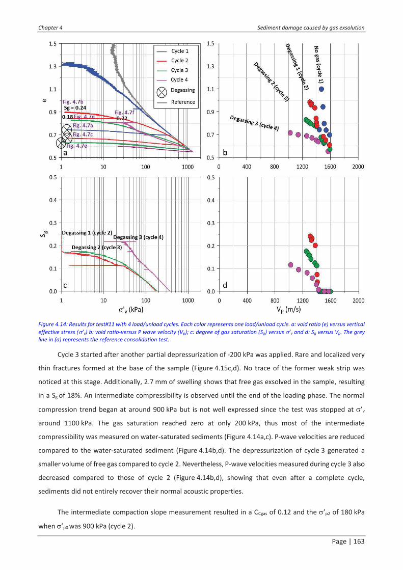
Chapter 4 Sediment damage caused by gas exsolution
Page | 163
Figure 4.14: Results for test#11 with 4 load/unload cycles. Each color represents one load/unload cycle. a: void ratio (e) versus vertical
effective stress (s�v) b: void ratio-versus P wave velocity (Vp); c: degree of gas saturation (Sg) versus s�v and d: Sg versus Vp. The grey
line in (a) represents the reference consolidation test.
Cycle 3 started after another partial depressurization of -200 kPa was applied. Rare and localized very
thin fractures formed at the base of the sample (Figure 4.15c,d). No trace of the former weak strip was
noticed at this stage. Additionally, 2.7 mm of swelling shows that free gas exsolved in the sample, resulting
in a Sg of 18%. An intermediate compressibility is observed until the end of the loading phase. The normal
compression trend began at around 900 kPa but is not well expressed since the test was stopped at s�v
around 1100 kPa. The gas saturation reached zero at only 200 kPa, thus most of the intermediate
compressibility was measured on water-saturated sediments (Figure 4.14a,c). P-wave velocities are reduced
compared to the water-saturated sediment (Figure 4.14b,d). The depressurization of cycle 3 generated a
smaller volume of free gas compared to cycle 2. Nevertheless, P-wave velocities measured during cycle 3 also
decreased compared to those of cycle 2 (Figure 4.14b,d), showing that even after a complete cycle,
sediments did not entirely recover their normal acoustic properties.
The intermediate compaction slope measurement resulted in a CCgas of 0.12 and the s�p2 of 180 kPa
when s�p0 was 900 kPa (cycle 2).

Chapter 4 Sediment damage caused by gas exsolution
Page | 164
Figure 4.15: Pictures of the sample during test 11. a: before the second depressurization (cycle 3, Figure 4.14a) showing the sediment
aspect before gas exsolution. b: after the second depressurization (Figure 4.14a). The sample swelled by 5 mm under the effect of gas
exsolution and small and rare fractures appeared along a pre-existing weak zone (lighter color). c: before the second depressurization
(cycle 3, Figure 4.14a) showing the sediment aspect before gas exsolution. d: after the second depressurization (Figure 4.14a). The
sample swelled by 2.5 mm under the effect of gas exsolution with rare and very thin fractures at the base of the sample. e: before the
third depressurization (cycle 4, Figure 4.14a) showing the sediment aspect before gas exsolution. f: after the third depressurization
(Figure 4.14a). The sample swelled by 3.5 mm under the effect of gas exsolution, swelling partly due to the numerous cm-long and
mm-thick fractures.
P-wave velocities have different trends with void ratio depending on the cycle (Figure 4.14b). Cycle 1,
where P-wave velocities were measured on water-saturated sediments, differs from the other cycles. The
impact of free gas on acoustic velocities is again displayed in this test as P-wave velocity trend with void ratio

Chapter 4 Sediment damage caused by gas exsolution
Page | 165
have a gentler slope when sediments contain free-gas (Figure 4.14b). Once Sg equals zero, P-wave velocities
are attenuated until reaching the normal compression trend (Figure 4.14a,b,c). Moreover, the cycle having
the biggest gas saturation is not the one displaying the smallest values of VP. Instead, P-wave velocities
decrease after each gas exsolution showing that sediments did not recover their normal acoustic response
after free gas disappeared and reloading.
Only two cycles were completed during test#5. The first cycle is not displayed in Figure 4.16a as the
pressure difference between the two ends of the sample was maintained during the whole cycle for
carbonated water circulation. Therefore, the calculated s�v for this cycle is not representative. However, total
depressurization completed on the sample (Du = -800 kPa), triggered a complete remolding of sediments as
shown in Figure 4.17. The sample fractured completely and so intensely that it resembled slurry. The total
swelling recorded was 9.5 mm, corresponding to gas saturation of 38%, which is the maximum value obtained
in this study. For this reason, test#5 is regarded as the extreme scenario. Two intermediate compressibilities
were measured. The first one corresponds to the fracture closing and has a sub-vertical slope (Figure 4.16a).
The second one has a slope greater than the virgin compaction curve. Finally, from s�v = 150 kPa to the end
of the loading, sediments follow the normal compression trend (grey line in Figure 4.16a). The normal
compressibility was recovered when Sg was already equal to zero for 50 kPa (Figure 4.16a,c). However,
normal compression trends on other tests were recovered with a larger delay from free gas disappearance
even though they displayed a lower gas saturation.
P-wave velocities were recorded throughout the two cycles. Figure 4.16c,d clearly shows the
difference in velocity magnitudes before and after exsolution. P-wave velocities recorded after exsolution
decreased by more than 50% for high void ratios (e > 1). After gas disappearance (s�v > 100 kPa, Figure 4.16c),
P-wave velocity for cycle 2 quickly increases with decreasing void ratio and recovers a trend parallel to the
water-saturated reference when the minimum void ratio for cycle 1 is exceeded (Figure 4.16b). Therefore,
gas exsolution seems to disturb P-wave velocities even after all the free gas has disappeared.
The slopes for the two intermediate compressibilities were measured. The closing of fractures
corresponds to a slope CCfrac of 1.6. The intermediate compressibility slope, CCgas, was measured at 0.5.
Therefore, a s�p1 of 42 kPa was calculated, the initial preconsolidation pressure, s�p0, being around 60 kPa.
s�p2 was not calculated as the classical method for its determination is not applicable in this case. However,
due to the slurry aspect of the sample after gas exsolution (which led to the maximum measured Sg of this
study) and based on how the compaction curve fits the reference, this test is considered as representative of
a critical remolded state where the sediment has entirely lost its preconsolidation pressure. We consider, for
this test, s�p2 = 0.

Chapter 4 Sediment damage caused by gas exsolution
Page | 166
Figure 4.16: Results for test#5 with 2 load/unload cycles. Each color represents one load/unload cycle. a: void ratio (e) versus vertical
effective stress (s�v) b: void ratio-versus P wave velocity (Vp); c: degree of gas saturation (Sg) versus s�v and d: Sg versus Vp. The grey
line in (a) represents the reference consolidation test.
Figure 4.17: Pictures of the sample during test 5. a: before complete depressurization (Figure 4.16a) showing the sediment aspect
before gas exsolution. b: after complete depressurization (Figure 4.16). The sample swelled by 9.5 mm under the effect of gas
exsolution. Numerous fractures generated and sediments took a slurry aspect.
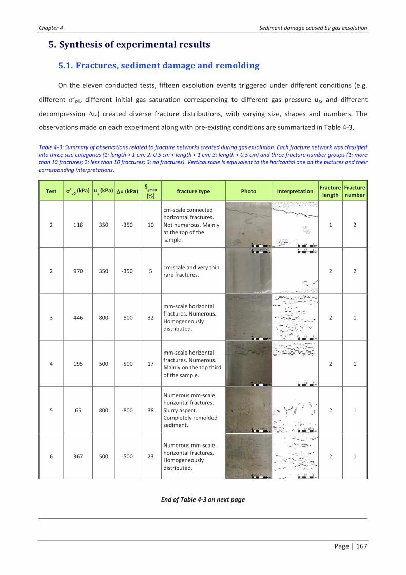
Chapter 4 Sediment damage caused by gas exsolution
Page | 167
5. Synthesis of experimental results
5.1. Fractures, sediment damage and remolding
On the eleven conducted tests, fifteen exsolution events triggered under different conditions (e.g.
different s�p0, different initial gas saturation corresponding to different gas pressure ug, and different
decompression Du) created diverse fracture distributions, with varying size, shapes and numbers. The
observations made on each experiment along with pre-existing conditions are summarized in Table 4-3.
Table 4-3: Summary of observations related to fracture networks created during gas exsolution. Each fracture network was classified
into three size categories (1: length > 1 cm; 2: 0.5 cm < length < 1 cm; 3: length < 0.5 cm) and three fracture number groups (1: more
than 10 fractures; 2: less than 10 fractures; 3: no fractures). Vertical scale is equivalent to the horizontal one on the pictures and their
corresponding interpretations.
Test s'p0
(kPa) ug
(kPa) Du (kPa) S
gmax
(%) fracture type Photo Interpretation
Fracture
length
Fracture
number
2 118 350 -350 10
cm-scale connected
horizontal fractures.
Not numerous. Mainly
at the top of the
sample.
1 2
2 970 350 -350 5 cm-scale and very thin
rare fractures.
2 2
3 446 800 -800 32
mm-scale horizontal
fractures. Numerous.
Homogeneously
distributed.
2 1
4 195 500 -500 17
mm-scale horizontal
fractures. Numerous.
Mainly on the top third
of the sample.
2 1
5 65 800 -800 38
Numerous mm-scale
horizontal fractures.
Slurry aspect.
Completely remolded
sediment.
2 1
6 367 500 -500 23
Numerous mm-scale
horizontal fractures.
Homogeneously
distributed.
2 1
End of Table 4-3 on next page

Chapter 4 Sediment damage caused by gas exsolution
Page | 168
Test s'p0
(kPa) ug
(kPa) Du (kPa) S
gmax
(%) fracture type Photo Interpretation
Fracture
length
Fracture
number
7 398 800 -400 20
cm-scale horizontal
fractures. Not
numerous. Sample is
cut into two parts.
1 2
8 405 800 -300 11 No visible fractures. 3 3
8 995 500 -500 36 Numerous cm-scale
horizontal fractures.
1 1
9 408 800 -100 5 No visible fractures. 3 3
9 895 700 -250 17 No visible fractures.
3 3
11 398 800 -200 24
Few mm-scale fractures
distributed along a pre-
existing light color
horizontal layer.
Light area thickens
during exsolution.
3 2
11 806 600 -200 18
Few mm-scale to cm-
scale fractures, mm-
thick in the bottom
edge of the sample.
2 2
11 1071 400 -400 22
Numerous cm-scale
fractures. Higher
fracture number and
thicker fractures on the
top half of the sample.
1 1
An empirical classification of fractures was defined based on the sample visible surface after
exsolution. Based on the observations in Table 4-3, fractures generated by gas exsolution are classified in
three different length categories:
1- Fractures longer than 1 cm
2- Fractures between 1 cm and 0.5 cm long
3- Fractures shorter than 0.5 cm.
Conversely, number of visible fracture are arbitrarily classified as:

Chapter 4 Sediment damage caused by gas exsolution
Page | 169
1- More than 10 visible fractures
2- Less than 10 fractures
3- No visible fractures.
This classification is empirical and the number of fractures is underestimated as only the sample
surface is visible. Nevertheless, as the same classification was applied to all fracture networks, comparison
between tests is considered as representative of the actual volume density.
5.2. Effect of gas exsolution on P-wave velocity
The effect of free gas on the acoustic properties of marine sediments has been already widely studied
(Helgerud et al., 1999; Rebata-Landa et al., 2012; Sultan et al., 2012). Helgerud et al. (1999), based on
previous works by Dvorkin et al. (1999) on elasticity of marine sediments, proposed an effective medium
model to predict P-wave and S-wave velocities in sediments containing free gas and/or gas hydrates based
on mineralogy, compressibility and initial void ratio.
We used this model to draw a chart for predicted P-wave velocity variation with void ratio for different
values of Sg (black lines in Figure 4.18a,b). The properties of sediments used in the modeling are summarized
in Table 4-1 (mass% of minerals, CC). The average number of contacts per grain in a bulk unit (called n in the
Helgerud et al. (1999) model) was taken as equal to 4. The mineralogy was simplified into three poles (clays,
quartz and carbonates) and is indicated in Table 4-1.
The P-wave velocities obtained from this study were plotted on the theoretical chart (Figure 4.18a,b).
Two variables are considered in Figure 4.18: the degree of gas saturation (Figure 4.18a) and the maximum
degree of gas saturation for each cycle (Figure 4.18b). Figure 4.18 also displays two examples of signals that
are considered reliable for the VP determination: one with a high degree of gas saturation, after gas
exsolution (Figure 4.18c), the other on a water-saturated and undisturbed sample, before gas exsolution
(Figure 4.18d).
The first observation is the good agreement between the curve corresponding to Sg = 0% on the chart
and the P-wave velocity measurements obtained before exsolution (Figure 4.18a). Once exsolution occurs,
P-wave velocities decrease drastically even for low values of Sgmax (red and blue crosses on Figure 4.18b). For
the highest values of Sgmax, this decrease reaches 75% of the water-saturated value for a given void ratio.
During the loading stage following exsolution, free gas is dissolved or expelled from the sample and Sg
decreases. Accordingly, P-wave velocities increase once again (Figure 4.18a). Once Sg reaches zero, P-wave
velocities remain below the reference values and follow a trend between the curve corresponding to Sg = 0%
and Sg = 2.5% (Figure 4.18a).

Chapter 4 Sediment damage caused by gas exsolution
Page | 170
Figure 4.18: P-wave velocity (VP) versus void ratio (e). Colors stand for (a) Sg (%) and (b) Sgmax (%). Black lines correspond to the
evolution of VP with e for different values of Sg based on the effective medium theory modeling (Helgerud et al., 1999). (c) is the typical
signal after gas exsolution, (d) is the typical signal after gas exsolution. Red line correspond to the source signal, green line is the
received signal.
5.3. Effect of degree of gas saturation on sediment compressibility
During the tests completed during this study, a clear difference in sediment compressibility was
observed when comparing the state before and after gas exsolution. The compressibility after gas exsolution
has a slope comprised between CC and CS called CCgas. When fractures were abundant and/or large enough, a
first compressibility state was observed with slopes generally larger than CC and called CCfrac.
For a comparative analysis, values of CCgas and CCfrac obtained from the different tests were plotted
against the maximum degree of gas saturation determined during each loading/unloading cycle (Sgmax) and
were then compared to CC and CS of water-saturated sediments (Figure 4.19). CCgas are all comprised between
the CC and the CS of water-saturated sediments.
CCfrac values, except for two cases, are much larger than the CC of water-saturated sediments. This
compressibility slope, observed after fracture initiation, corresponds to fracture closing. CCfrac obtained from
tests 7 and 11 are lower than CC. Test 7 fracture network is unique as a large fracture split the sample in half
(Table 4-3), and contact between the two halves occurred when the fracture closed. For test 11, the fracture
network is one of the densest, with centimeter-scale fractures. Before reloading (cycle 4), a permeability

Chapter 4 Sediment damage caused by gas exsolution
Page | 171
measurement under an imposed vertical hydraulic gradient partially closed the thinner fractures. This could
be an explanation for the lower values of CCfrac obtained on both tests.
Figure 4.19: Compressibility versus Sgmax (%). Two type of compressibility are displayed. The grey vertical lines stand for the water-
saturated sediments CC and CS, the dotted lines being the maximal and minimal values obtained during the different tests. Values of
CCfrac are annotated as labels, since values above 0.5 were plotted at 0.5 to condense the graph.
5.4. Hydraulic conductivity versus degree of gas saturation
Hydraulic conductivity (K) data versus void ratio are shown in Figure 4.20a. K values obtained on the
same sediment using the classical falling head method are plotted for comparison.
K measurements made before exsolution on water-saturated samples fit well with odometer
measurements (Figure 4.20a). After gas exsolution, K increases above the water-saturated sample trend.
Thereafter, K decreases rapidly during the beginning of reloading and reaches values below the trend of
water-saturated samples. This decrease happened during a short time interval compared to the decrease of
K during consolidation of the water-saturated sample. However, some of the K values acquired on water-
saturated sediments seem to spread relatively to the trend curve in the same way. Nevertheless, Figure 4.20b
clearly shows that K increases with the Sg.

Chapter 4 Sediment damage caused by gas exsolution
Page | 172
Figure 4.20: a: hydraulic conductivity, K (m/s) versus void ratio. The blue dashed line is an exponential fit for hydraulic conductivities
on water-saturated sediments obtained from oedometers (blue crosses). b: K (m/s) versus Sg (%).
5.5. Preconsolidation pressure evolution with degree of gas saturation
In this paper, two preconsolidation pressures were determined. Before fracture closing, the
intersection between the two slopes corresponding to CCfrac and CCgas gives the s�p1. After fracture closing, s�p2
was determined by the intersection of the swelling curve and the virgin compaction curve.
Figure 4.21: Preconsolidation ratio versus Sgmax (%). a: ratio between preconsolidation pressures calculated before fracture closing,
s�p1, and the initial preconsolidation pressure, s�p0. The labels correspond to the fracture classification given in Table 4-3."�s�"stands"
for"the"fracture"length,"�d�"for"the"fracture number. b: ratio between preconsolidation pressures calculated after fracture closing, s�p2,
and the initial preconsolidation pressure, s�p0. Values from Sultan et al. (2012) are also plotted as comparison (red crosses). An
exponential fit of the study results shows a strong determination coefficient (R²).

Chapter 4 Sediment damage caused by gas exsolution
Page | 173
To compare the two parameters over the entire set of test results, we normalized them with respect
to s�p0 (Figure 4.21). The s�p1/s�p0 increases generally with increasing Sgmax but without a clear tendency
(Figure 4.21a). Moreover, comparing these values to fractures in Table 4-3 shows that there is no clear
relationship between fracture size and number and s�p1/s�p0.
Regarding the ratio between s�p2 and s�p0, results show that it decreases with increasing Sgmax,
evidencing a preconsolidation pressure degradation with Sgmax (Figure 4.21b). As a comparison, values from
the study by Sultan et al. (2012) on gassy sediments from the Gulf of Guinea were also added to Figure 4.21b.
The results show a clear logarithmic trend with a strong determination coefficient of 0.75 and starting with
a ratio equal to 1 when Sg is zero. Values from the Gulf of Guinea are not exactly on the proposed trend. They
were obtained on sediments having a completely different behavior in a water-saturated state, with a CC as
high as 2 (Colliat et al., 2011).
6. Discussion
6.1. Fracture size and number: main controlling factors
The classification of fractures depending on their size and number was compared to the other
parameters used or obtained during the testing program (e.g. s�p0, Du or Sgmax; Table 4-3). The aim is to
identify the main parameters controlling fracture size and number.
First, the length of fractures formed during this study range from one mm to few cm. Their observable
thicker part corresponds to the center of the crack. Boudreau (2012) shows that growth and rise of gas
bubbles in sediments is possible through fracture generation and that bubbles will be disk-shaped (also
demonstrated by Katsman (2015)). Shin and Santamarina (2011) as well as Jain and Juanes (2009) show that
gas-driven fractures are favored in fine-grained sediments. Therefore, gas exsolution and subsequent bubble
generation and growth explains the shape of fractures. The observed cracks are not pre-existing
discontinuities.
It clearly appeared during our study that the Sgmax controls the fracture number. The larger the volume
of free-gas generated, the bigger the number of fractures. However, some exceptions, like with test#11, show
that this is not the unique controlling factor for fracture number. A secondary parameter, the magnitude of
depressurization (Du), seems to participate in controlling fracture number. The higher Du, the more
numerous the fractures. The two parameters are closely related as the Sg, corresponding to a volume of free
gas generated during exsolution, is a direct consequence of the magnitude of depressurization.
From visual observations, three main fracture distributions can be discriminated (Table 4-3): dense and
small fractures (tests 3, 4, 5 and 6), dense and large fractures (tests 8 and 11), and rare or inexistent fractures
(tests 2, 8, 9, and 11).

Chapter 4 Sediment damage caused by gas exsolution
Page | 174
The two denser distributions correspond to high Sgmax values (more than 20%) reached by complete
depressurization. Test#4 is an exception. It presents a very dense fracture network but only at the top of the
sample. The sample was clearly not entirely saturated with carbonated water hence explaining fracture
distribution. Besides, Sgmax is calculated for the complete sample. Thus, applied to the fractured volume, Sgmax
is much higher than calculated. Smaller Sgmax or partial depressurization lead to fracture networks with few
or no fractures at all.
Preconsolidation pressure (s�p0) is the controlling factor of fracture size. Observation of the two groups
with dense fracture networks (high Sgmax) shows that when s�p0 is small (below 500 kPa) fractures are small.
For higher s�p0 (above 500 kPa), these fractures get longer and thicker. Various studies on bubble growth and
shape in marine sediments yielded the same results. Boudreau et al., (2005), Barry and Boudreau (2010) and
Katsman, (2015) demonstrate that bubble shape and size is mainly controlled by the mechanical properties
of sediments. In particular, Katsman (2015) concludes that bubbles generating in weak sediments are small
with higher surface-to-volume ratio (thin bubbles) while bubbles forming in stronger sediments tend to be
larger and more spherical (larger).
Therefore, the controlling factors for fracture network architectures are Sgmax and Du both controlling
the number of fractures while s�p0 controls the size of the fractures.
6.2. Gas exsolution/expansion: a permanent P-wave velocity
attenuation?
The presence of free gas has been always an issue when dealing with P-wave velocities (Sills et
al., 1991; Helgerud et al., 1999; Sultan et al., 2012). It provokes strong attenuation of the signal, ultimately
preventing any signal propagation. Therefore, P-wave velocities are often used as a tool to detect free gas
formation (Rebata-Landa et al., 2012; Sultan et al., 2012) as well as for estimating a degree of gas saturation
(Lee & Collett, 2006; Morgan et al., 2012). The acoustic response of gassy sediments is theoretically supposed
to join the trend of saturated sediments whenever Sg becomes equal to zero.
The present study confirms this attenuating effect of free gas on P-wave velocities (Figure 4.18). The
higher the Sg, the stronger the P-wave velocity attenuation. Besides, as free gas is dissolved and compressed
during reloading, P-wave velocities increase once again. It shows the strong correlation between P-wave
velocities and the Sg. Nevertheless, during reloading, when Sg reaches zero, P-wave velocities remain
attenuated compared to the normal trend for water-saturated sediments (Figure 4.18a). Therefore, the
damage generated by gas exsolution seems to delay the normal acoustic response of the sample.
The presence of fractures is a known factor for attenuating P-wave velocities in the perpendicular
direction, independently of its filling material (Anderson et al., 1974; Kahraman, 2002; Leucci & Giorgi, 2006;
Popp & Salzer, 2007). Fracture generation may have triggered local changes in the shear modulus and/or the
Chapter 4 Sediment damage caused by gas exsolution
Page | 175
bulk modulus of the sediment (Huang et al., 1995). Therefore, even after mechanical reloading and water
saturation, long-term impact of fractures on the acoustic response is expected.
Moreover, Helgerud�s model, predicting P-wave velocities for given Sg�s (Helgerud et al., 1999), does
not fit with most of the P-wave velocities recorded after gas exsolution (Figure 4.18a). P-wave velocities are
greatly overestimated (up to 300 m/s) for samples where dense fracture networks appeared during gas
exsolution (Table 4-3) and they are underestimated (less than 100 m/s) for samples presenting rare or no
fractures after gas exsolution (Table 4-3). P-wave velocities measured on samples with a higher degree of gas
saturation present a signal that can be misleading. This may lead to errors in measurement that partly explain
the differences observed with the model (#100 m/s). Considering the potential errors in measuring P-wave
velocities for gassy samples, the Helgerud model is in adequacy with the measurements made on samples
without or with rare fractures. The impact of fractures and discontinuities in the sample over P-wave
velocities is responsible for the rest of the discrepancy, as modeled values are calculated for a homogeneous
medium.
Thus, sediment damage caused by gas exsolution (through fractures, or with no visible markers), seems
to have a durable impact on acoustic properties of sediments.
6.3. Gas exsolution/expansion effects on sediment compressibility
Sultan et al. (2012) have clearly identified the impact of gas exsolution on the compressibility of clayey
sediments. Experimental data of Sultan et al. (2012) showed that after gas exsolution, the compressibility of
the sediments decreased significantly and is between the swelling index and the compression index of the
initial intact sediments. This compressibility degradation was interpreted as being the result of sediment
damaging during free gas generation. Previous experiments also highlighted a decay of compressibility with
the presence of gas bubbles in soft marine clays (Sills et al., 1991; Nava Castro et al., 2013; Liu et al., 2016).
They concluded that gas bubbles bear part of the load applied on the sample and that soil compressibility
measured on gassy sediment is primarily due to bubble compression and secondarily due to normal sediment
compression, implying water expulsion. The presence of free gas in sediments was also proved to be
responsible for a delay in consolidation. As gas escapes or dissolves, consolidation happens faster (Sills et al.,
1991; Nava Castro et al., 2013).
This study showed that gas exsolution creates two intermediate compressibilities after fracture
generation (CCfrac and CCgas) and only one when no fractures appeared (CCgas) (Figure 4.12a, Figure 4.14a and
Figure 4.16a). The formation of fractures strongly impacted the compressibility of sediments. CCfrac were only
measured for dense fracture networks and were generally higher than CC (Figure 4.19). Conversely, fracture
number affected the compressibility after fracture closure (CCgas). For equivalent Sgmax, higher CCgas were
recorded for higher number of fractures (Table 4-3 and Figure 4.19). CCgas was always comprised between CC
and CS (Figure 4.19).

Chapter 4 Sediment damage caused by gas exsolution
Page | 176
Nevertheless, CCgas were also measured when no fractures were generated in the sediments. This
shows that if fractures have an impact on the compressibility of sediments, the main controlling factor is the
presence of gas. Indeed, this study shows that when Sgmax increases, CCgas increases (Figure 4.19). For low
Sgmax, CCgas is closer to the swelling index of water-saturated sediments. This correlation was also noted by
Hight and Leroueil (2003) during loading of a sample with occluded gas bubbles. Therefore, gas exsolution
tends to destroy the elastic behavior of sediments.
Test#5 displayed an extreme behavior with a slurry aspect after gas exsolution and a CCgas higher than
CC. The virgin compaction curve was reached very fast compared to other tests (Figure 4.16a) showing that,
after gas exsolution in test#5, the sediments behaved as the initial remolded sediment.
Moreover, compressibility recovers a normal trend once s�p0 is reached, long after Sg reached zero.
Hight and Leroueil (2003) demonstrated that once gas bubbles collapsed during reloading of a sample
containing occluded gas bubbles, it recovers its normal CC. The difference in this study is that free gas is
concentrated along fracture planes and is not in the form of occluded gas bubbles. Therefore, as for P-wave
velocity attenuation, the delay in compressibility recovery may be due to a permanent impact of fractures
and damage caused by gas exsolution.
6.4. Gas exsolution/expansion effects on sediment permeability
Permeability of sediments can be affected by several mechanisms. Normal consolidation of sediments
provokes a decrease in hydraulic conductivity (Olsen, 1960; Chu et al., 2002). The presence of fractures may
enhance this permeability depending on the fracture orientation relative to hydraulic gradient (Alfaro &
Wong, 2001). Besides, free gas in fine-grained sediments were proved to be a factor for permeability
reduction (Egermann & Vizika, 2000; Naylor et al., 2000; Hight & Leroueil, 2003; Jang & Santamarina, 2014).
If free gas accumulates in clayey layers, a capillary seal may form (a gas cap), generating an effective
permeability even lower than the intrinsic permeability of the clayey layer (Revil et al., 1998; Cathles, 2001).
Gas exsolution triggered the formation of horizontal millimeter to centimeter-scale fractures. Their
orientation corresponds to a direction orthogonal to the possible fluid expulsion, which is not favorable to
an increase in permeability. However, as observation of the fracture network was only possible at the sample
surface, it is possible that fluid pathways created through connections between fractures, thus explaining the
observed increase in permeability right after gas exsolution (Figure 4.20). These fractures were filled with
free gas after gas exsolution, which may rather be a parameter in favor of a decrease in permeability.
However, we do observe an increase in sample permeability just after fracture creation showing that gas
filling the fractures may be in a continuous phase through an interconnected fracture network (Jang &
Santamarina, 2014).

Chapter 4 Sediment damage caused by gas exsolution
Page | 177
During reloading, the rapid decrease in permeability (Figure 4.20) is probably related to the closing of
fractures, and the consequent reduction of fluid pathways. Consequently to fracture closing, trapping of free
gas in reduced areas changes free-gas distribution from a continuous phase to a more discrete distribution,
a factor that was proved by Jang and Santamarina (2014) to reduce sample permeability. The creation of
potential capillary seals along the former fracture planes could explain the hydraulic conductivity values that
are below the normal trend (Cathles, 2001).
Therefore, gas exsolution provokes an increase in permeability through fracture creation, creating
preferential pathways. Then, reloading quickly reduces permeability due to fracture closure and capillary
sealing as a consequence of free gas being captured in a discrete distribution.
6.5. Gas exsolution/expansion effects on preconsolidation pressure and
the consequence in terms of shear strength
Besides the fracture formation that has already been discussed, gas exsolution has an impact on the
preconsolidation pressure of sediments, showing the degree of sediment damage caused.
Before fracture closing, the degradation of sediment preconsolidation pressure is significant but seems
to decrease with Sgmax (Figure 4.21a). However, no clear trend appears. Except for one value, corresponding
to test#5, all the ratios are below 0.35. It tends to indicate that at 35% of the s�p0 fractures are closed as s�p1
indicates a degradation connected to fracture closing. The sample of test#5 was completely fractured during
gas exsolution explaining the high value for the s�p1/s�p0 ratio: fractures took more time to close.
s�p2 was measured after fracture closing, therefore it evaluates the part of sediment damage that is
visually imperceptible. The ratio between s�p2 and s�p0 correlates with Sgmax through a logarithmic law
(Figure 4.21b): the bigger Sgmax, the more the sediment was remolded, recording a decrease in
preconsolidation pressure. This type of relation was already noted on sediments from the Gulf of Guinea
(Sultan et al., 2012) but at lower Sgmax (below 10%). Besides, several other studies demonstrated this decrease
in presconsolidation pressure with an increasing degree of gas saturation (Lunne et al., 2001; Hight et
al., 2002). For Hight and Leroueil (2003), it is mainly the result of damage due to bubble-growth in the
sediments, the degree of damage being related to the initial level of structure. The initial level of structure
may be the explanation for the differences observed between the measurements made during this study and
the results obtained by Sultan et al. (2012) on a different sediment.
This study showed, for different sediments and at a higher Sgmax that a complete loss of
preconsolidation pressure is feasible. For 38% of Sgmax, preconsolidation pressure was completely lost,
showing that sediments were entirely remolded by gas exsolution. The corresponding sample (test#5) had a
slurry aspect right after gas exsolution and displays extreme behavior in terms of compressibility and
sediment damage.

Chapter 4 Sediment damage caused by gas exsolution
Page | 178
Therefore, the experimental results confirm that gas exsolution causes sediment damage and
remolding. For strong gas exsolution, leading to high Sgmax, sediments can even reach a state where they
entirely lose their preconsolidation pressure.
Wheeler (1988) showed that methane bubbles might decrease or increase the undrained shear
strength of reconstituted silty-clay samples. This was shown to depend on the level of total and effective
stress. In the Wheeler (1988) experiments, gas bubbles were formed artificially by using the zeolite molecular
sieve technique. Gas naturally formed in sediments or was generated by circulation of carbonated water.
Subsequent decompression was shown to negatively affect the undrained shear strength. Lunne et al. (2001),
Hight, Hamza and El Sayed (2002) and Sultan et al. (2012) all point out that the degree of gas saturation
significantly reduces preconsolidation pressure and shear strength.
Sultan and Garziglia (2014) proposed a constitutive model to simulate the mechanical behavior of gassy
sediments where preconsolidation pressure is the main parameter controlling yield surface and therefore
shear strength of the sediment. By introducing to a conventional Cam Clay type model the �preconsolidation
pressure - degree of gas saturation� logarithmic relationship equivalent to the one shown in Figure 4.21b,
they were able to reproduce the observed data published by Lunne et al. (2001), Hight, Hamza and
El Sayed (2002) and Sultan et al. (2012). Data shown in Figure 4.21b highlight the important consequence of
gas formation on the shear strength of the sediment from the AMV where the damage due to bubble growth
may strongly decrease its shear strength. A Sgmax of 38 % seems to be the upper limit for complete destruction
of the structure and therefore the shear strength of AMV sediments and favoring mud formation.
7. Conclusions
This chapter investigates the impact of gas exsolution on the mechanical behavior of mud samples
recovered on mudflows expelled from the Absheron Mud Volcano. The goal was to understand the factors
that control sediment damaging and to quantify and determine the criteria by which we may determine that
sediments are completely remolded, and considered as changed into mud. Eleven consolidation tests using
a novel experimental apparatus allowed to generate free gas under different consolidation conditions.
Results show that:
1- The number of fracture generated through exsolution is controlled by the degree of gas
saturation while preconsolidation pressure mainly controls their length.
2- Gas exsolution provokes sediment damage (through fracture emplacement and loss of
preconsolidation pressure) and it increases with the degree of gas saturation while the elastic
modulus of sediments is partly lost. Shear strength is also expected to decrease as a consequence
of sediment damage.

Chapter 4 Sediment damage caused by gas exsolution
Page | 179
3- Acoustic response remains degraded long after free gas has entirely disappeared from the
sample. Compressibility is also durably modified, reaching normal trends only when initial
preconsolidation is exceeded. Permeability first increases through fracture creation, but quickly
deteriorates due to the presence of gas leading to capillary sealing during reloading. Therefore,
sediments do not recover entirely from gas exsolution damage during reloading.
4- During testing, critical behavior was observed for a degree of gas saturation of 38%. Gas
exsolution triggered complete remolding of sediments (entire loss of preconsolidation pressure
and therefore its shear strength) that took a slurry aspect. The same test displayed the highest
compressibility at the beginning of reloading. Its compressibility trend was close to the initial
compaction behavior while sediments had not yet compacted. Therefore, gas exsolution alone
was able to generate mud from compacted sediments.
Our experimental results show that gassy sediments with a discontinuous gas phase may take place
for Sg greater than 15 %. We show that such an experimental study can help determine the criteria for mud
formation under laboratory conditions and on a particular sediment sample: mud expelled from the
Absheron Mud Volcano. These criteria can be implemented into numerical models, integrating mechanical
behavior under the geological conditions observed and determined in the field. Ultimately, this experimental
study offers a unique opportunity to quantify the volume of gas required to generate the volume of mud at
depth that was extruded to form the observed Absheron Mud Volcano.

Chapter 4 Sediment damage caused by gas exsolution
Page | 180

Page | 181
Chapter 5: From stratified sediments to fluid mud generation
Abstract
The Absheron Mud Volcano area in the South Caspian Basin offers a unique multidisciplinary dataset
that led to develop a conceptual formation model. This model mainly relies on hydrofracturing of
overpressured strata saturated with dissolved gas, leading to gas exsolution in under-compacted and
evaporite-rich layers, generating overpressured mud driven to the seafloor through density inversion and gas
expansion. Through laboratory testing, gas exsolution in compacted marine sediments leads to significant
sediment damage (loss of preconsolidation pressure and decrease of shear strength), eventually forming
completely reworked material like the mud expelled at the volcanoes. The integration of geological
observations, in situ physical parameters, sediment properties and empirical behavior of sediments with gas
exsolution into 2D diffusion models allowed to simulate the geological and physical conditions required to
generate mud at depth at the Absheron location. The integration of the Anhydritic Surakhany Formation
acting as a regional seal and of faults with sealing capacities are important parameters in order to trigger
hydrofracturing. Moreover, the mud remobilization towards the surface was also modeled through modified
Navier-Stokes equations considering gas expansion impact on mud density. From simulations it transpires
that mud would be extruded after 100 years when considering only density inversion.

Page | 182

Page | 183
Chapitre 5 : Génération de boue fluide à partir de sediments stratifiés
Résumé
La zone du volcan de boue d�Absheron, dans le Bassin sud caspien, offre un jeu de données
multidisciplinaire unique ayant déjà permis d�en proposer un modèle de mise en place. Dans ce modèle,
l�hydrofracturation de strates en forte surpression et saturées en gaz dissous déclenche l�exsolution du gaz
contenu dans des couches sous-compactées et riches en évaporites, ce qui génère de la boue en surpression
qui remonte jusqu�au fond marin par inversion de densité et expansion des bulles de gaz. Par ailleurs, des
essais en laboratoire ont démontré que l�exsolution du gaz dans des sédiments marins compactés provoque
un endommagement considérable de ces sédiments (perte de leur pression de préconsolidation et
diminution de la résistance au cisaillement) menant potentiellement à un matériel complétement remanié
comme la boue des volcans. L�intégration des observations géologiques, des propriétés physiques in situ, des
propriétés des sédiments et des lois de comportement empiriques des sédiments après exsolution du gaz
dans un modèle régional de diffusion 2D a permis de définir les conditions nécessaires pour la génération de
boue en profondeur dans la zone d�Absheron. L�intégration de la Formation du Surakhany Anhydritique
agissant comme une couverture régionale ainsi que la prise en compte de failles jouant le rôle de barrières
de perméabilité horizontale sont des paramètres nécessaires afin de déclencher l�hydrofracturation. La
remontée de la boue vers la surface a également été modélisée par le biais d�équations de Navier-Stokes
modifiées afin de prendre en compte l�effet de l�expansion du gaz sur la densité. Ces simulations montrent
qu�en ne considérant que l�inversion de densité, la boue prendrait une centaine d�années pour atteindre la
surface.

Page | 184

Chapter 5 From stratified sediments to fluid mud generation
Page | 185
1. Introduction
While extensive work has been focused for decades on mud volcano (MV) architecture and on gassy
sediments, few studies have numerically explored MV formation and evolution. Several authors have
attempted to reproduce visible structures and the morphological evolution of MVs through analogue models
(Woolsey et al., 1975; Nermoen et al., 2010; Mourgues et al., 2012; Dupuis, 2017; Odonne et al., in press).
The results provide understanding of the evolution of surface structures and morphology as well as exploring
possible subsurface mechanisms able to reproduce surface and subsurface features as observed in the field.
However, most of these models used non-cohesive materials to simulate fine-grained cohesive sediments
(Woolsey et al., 1975; Nermoen et al., 2010; Dupuis, 2017) following the theory on scaled models
(Hubbert, 1937) and therefore, the processes used to remobilize material in the models may be different
from those applying to natural MVs. Other authors developed numerical models to explain remobilization
and the subsurface mechanism for mud transport (Brown, 1990; Gisler, 2009; Zoporowski & Miller, 2009;
Collignon et al., 2018a). These models are based on physical, chemical and mechanical laws applied to natural
conditions, therefore approaching processes more accurately. However, these numerical models only assess
the fluid mud flow or the mechanical evolution of mud during its ascent. Deville et al. (2010) computed
regional fluid flow models in the Barbados prism and showed that MVs are located above overpressured
zones. Therefore, modeling of mud volcanoes focused on reproducing the observed structures or the mud
flow dynamics, while other studies looked into the the regional background to explain MV location. None of
the models integrated both the regional and local processes into a unique model. Moreover, the impact of
gas exsolution and expansion on the behavior of the mud flow is often ignored or simplified.
The AMV has been densely surveyed for hydrocarbon exploration purposes and for geohazard
assessment (Contet & Unterseh, 2015; Gautherot et al., 2015; Unterseh & Contet, 2015; Dupuis, 2017) giving
a dense and high-quality multidisciplinary dataset. The SCB is also densely studied, and several subsidence,
thermal and fluid-flow models provide understanding of regional scale phenomena. Overall, existing data
present a unique opportunity to model and simulate the formation of a mud volcano within its geological
background. Preliminary modeling work was conducted in order to explain the location of the AMV at the
crest of the Absheron anticline, coupling sedimentation-related overpressure generation and 2D-diffusion
equations for fluid flow and methane accumulation (Chapter 3:4.4; Blouin et al., 2019). It showed that the
AMV was formed at the location where critical overpressure (near-fracture conditions) affected methane-
saturated areas. However, hydrofracturing conditions were not reached solely through sedimentation and
with the geological structure modeled in Chapter 3:4.4.
The present chapter assesses the following main two questions:

Chapter 5 From stratified sediments to fluid mud generation
Page | 186
· Is it possible to simulate mud generation conditions at depth by considering mechanical
properties of sediments, sedimentation rates, structural elements and the impact of gas
exsolution?
· Is the sole impact of gas expansion on the mud properties able to drive mud up to the
seafloor?
Hereafter, we present the improvements brought to the 2D-diffusion model by considering a low-
permeability interval corresponding to the Anhydritic Surakhany Formation and by integrating fracture
generation conditions, gas exsolution and sediment damage (Chapter 4:5.5); these make it possible to
propose a possible geological and physical setting and a chain of processes leading to mud generation.
Modified Navier-Stokes equations accounting for gas bubble expansion and changes in mud properties
(density and pressure) were used in order to simulate mud ascension through the sedimentary strata.
2. Material and methods
2.1. Mud generation
The method used to characterize sediment properties (including compressibility and hydraulic
conductivities) of the modelled stratigraphic layers was already discussed in Chapter 2:3.2.4. The software
used to calculate the sedimentation-related overpressure (SeCoV3 Ifremer in-house software) was described
in Chapter 2:3.4.1 and Chapter 3:3.4.1 and no further developments were done in the following modeling
work.
The geometrical model, based on work by Green et al. (2009), was slightly modified (Figure 5.1) to take
into account the Anhydritic Surakhany Formation (ASF, see Chapter 2:1.1.2 and Chapter 3:4.3). The fault
network geometry is based on seismic interpretation (Chapter 3:4.1). In order to decrease the calculation
time, the resolution was reduced by considering a vertical increment equal to 192 m with a total of 50 vertical
nodes, and a horizontal increment equal to 244 m with a total of 225 horizontal nodes (Figure 5.1).
The 2D-diffusion software was modified in order to consider two additional phenomena:
hydrofracturing and gas compressibility and exsolution (Boyle�s and Henry�s laws). In a context where the
maximum principal stress is vertical (s1 = sv), hydrofracturing is vertical and occurs when and where the fluid
pressure is exceeding the sum of the tensile strength of the host sediment and the minimum horizontal stress
(s3). For the purpose of modeling, a realistic approximation is to consider that hydrofracturing occurs for a
given ratio between overpressure and vertical effective stress (Du/s�v), generally obtained from pressure logs
(see Figure 1.10, Chapter 1:2.5.1 for details). When the ratio Du/s�v reaches the critical condition,
hydrofractures are generated in the concerned area. As a working hypothesis, the hydrofractured area
permeability is calculated from the hydraulic conductivity laws (Eq. (4)) using a void ratio of 1. The methane
diffusivity (DC) of hydrofractured area is considered as being the same as faults. Fracture may trigger a
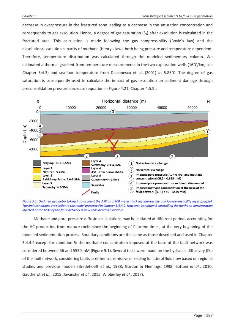
Chapter 5 From stratified sediments to fluid mud generation
Page | 187
decrease in overpressure in the fractured zone leading to a decrease in the saturation concentration and
consequently to gas exsolution. Hence, a degree of gas saturation (Sg) after exsolution is calculated in the
fractured area. This calculation is made following the gas compressibility (Boyle�s law) and the
dissolution/exsolution capacity of methane (Henry�s law), both being pressure and temperature dependent.
Therefore, temperature distribution was calculated through the modeled sedimentary column. We
estimated a thermal gradient from temperature measurements in the two exploration wells (16°C/km, see
Chapter 3:4.3) and seafloor temperature from Diaconescu et al., (2001) at 5.85°C. The degree of gas
saturation is subsequently used to calculate the impact of gas exsolution on sediment damage through
preconsolidation pressure decrease (equation in Figure 4.21, Chapter 4:5.5).
Figure 5.1: Updated geometry taking into account the ASF as a 300 meter thick incompressible and low-permeability layer (purple).
The limit conditions are similar to the model presented in Chapter 3:4.4.2. However, condition 5 controlling the methane concentration
injected at the base of the fault network is now considered as variable.
Methane and pore-pressure diffusion calculations may be initiated at different periods accounting for
the HC production from mature rocks since the beginning of Pliocene times, at the very beginning of the
modeled sedimentation process. Boundary conditions are the same as those described and used in Chapter
3:4.4.2 except for condition 5: the methane concentration imposed at the base of the fault network was
considered between 56 and 5550 mM (Figure 5.1). Several tests were made on the hydraulic diffusivity (Dh)
of the fault network, considering faults as either transmissive or sealing for lateral fluid flow based on regional
studies and previous models (Bredehoeft et al., 1988; Gordon & Flemings, 1998; Battani et al., 2010;
Gautherot et al., 2015; Javanshir et al., 2015; Wibberley et al., 2017).

Chapter 5 From stratified sediments to fluid mud generation
Page | 188
2.2. Mud ascent
The modeling of mud generation is complemented by the modeling of the ascent of the fluid mud. The
purpose of this model is to determine whether the mud mass is able to rise up to the seafloor through gas
expansion processes only.
To model the ascent of low-density mud, we combined two approaches: one solving the problem in
two dimensions at low viscosities (Tryggvason, 2012) and one for extrapolating the results to realistic higher
viscosities using one-dimensional calculations (Furbish, 1997). The 2D calculations were completed using the
Datarmor Ifremer supercomputer (PCDM, 2018) allowing to reduce significantly the time of calculation by
parallel processing. Simulations that would need a week on a PC, are completed on less than 24 hours using
Datarmor supercomputer.
The 2D approach models the mud as a one-phase fluid flow using simplified Navier-Stokes equations
(Eq. (11) and Eq. (12), see Chapter 2:3.4.4), taking into account gas compressibility through Boyles�s law.
Methane modifies the mass-density of the mud following Eq. (13) (Chapter 2:3.4.4) leading to mass-density
inversion between the mud generation zone and the host rock (Brown, 1990; Kopf, 2002; Deville, 2009;
Collignon et al., 2018a). Mud and host rocks are modelled as having the same viscosity, constant over time
and that does not vary with the presence of free gas. The methods of resolution using discretization of the
different terms of the simplified Navier-Stokes equations was adapted from Tryggvason et al. (2011). The
Navier-Stokes (NS) software used in this chapter is based on code1 of Tryggvason (2012).
Two modified versions of code1 were tested. The modifications were made at the Ifremer, for the
purpose of the study. The first version (code1 v1) applies directly the numerical resolution method of
Tryggvason (2012) by considering the gas exsolution and expansion phenomenon and by including the impact
of free gas in the computation on the mass-density evolution. The second version (code1 v2) considers an
initial mud overpressure due to the presence of free gas which varies with the gas expansion during mud
ascent.
The 2D simulation of mud ascent was completed over structural models with 100 nodes per 100 nodes
representing an area of 10 km in length and 4 km in depth corresponding to the approximate length of the
Absheron anticline in a SSW-NNE direction and to the depth below sea level of the mud generation zone. The
water column is considered and serves as an upper boundary limit where no exchange with the mud and
sediment zones is allowed. Therefore, the extrusion of mud and its behavior after reaching the surface is not
considered in the present work as it implies complex chemical and physical interactions between sea water
and formation water (Kopf, 2002; Etiope et al., 2009). The two lateral boundaries are considered as no
exchange boundaries. The sediment column presents a mass-density ranging from 2100 kg/m3 for the
deepest sediments to 1900 kg/m3 for the shallowest sediments. These values are calculated from porosities
at wells, derived from sonic data (see Chapter 2:3.3) and using a grain solid mass-density of 2650 kg/m3. An

Chapter 5 From stratified sediments to fluid mud generation
Page | 189
initial mud body is considered at the initial state as a convex-up half-disk corresponding to the volume of
damaged sediments calculated from the regional diffusion simulation and having the same mass-density as
unconsolidated marine sediments (1900 kg/m3). In code1 v2, this initial volume of mud has also an initial
overpressure which was obtained from diffusion simulations.
The mud generation process implies the formation of hydrofractures. This hydrofractures should
propagate vertically in the context of the extrados of the Absheron anticline where normal faulting was
observed. Therefore, vertical conduits having the same mass-density as the mud source can be introduced
in the initial geometry in order to simulate the potential presence of vertical fractures.
Viscosities measured for surface marine sediments highly depends on the type of sediments, but are
clearly below 10 5 kPa.s (Locat & Demers, 2008; Torrance, 2010; Jeong, 2013). However, this range of values
is not representative of highly consolidated and stratified sediments, whose typical values of viscosity exceed
10 14 kPa.s, value corresponding to evaporitic sediments (Mukherjee et al., 2010; Collignon et al., 2018b).
With the depth range and type of host sediment encountered here, taking realistic values leads to
exceedingly long computation times. The Lusi catastrophe provided the first direct monitoring of a mud
volcano initiation (Mazzini et al., 2012; Tingay et al., 2015, 2017). Tingay et al. (2017) proved using the BJP-1
well data and reports that the mud generation and its ascent from a depth of 1000 m happened within two
days. Following these observations (Tingay et al., 2017), the simulations were limited to the first 24 hours
after the mud generation, leading to calculations time on the supercomputer Datarmor of more than 30 days
for a viscosity of 10 7 kPa.s. This directly arises from the resolution method: the time increment depends on
the mesh resolution and on the viscosity. For instance, for a viscosity of 10 7 kPa.s and for the used mesh of
100 nodes per 100 nodes (mesh resolution of 100 m horizontally and 39 m vertically), a time increment dt of
10 � 5 s was needed in order to reach numerical convergence. This implies 1.7 x 10 9 calculations to simulate
the 24 hours of mud ascent. We therefore ran models based on Tryggvason (2012) over three orders of
magnitudes for viscosity (10 5, 10 6 and 10 7 kPa.s) and observed that the main change was with the timing,
other parameters of interest being insensitive to viscosity changes.
The extrapolation to more realistic viscosity values was completed by a simple 1D calculation following
a simple example of Furbish (1997) modeling a buoyant magma flow within a vertical dyke. It was possible to
calculate the velocity of the ascending mud using the equation:
{3|6 = " DaM 3\} $ \6@d~² $ |ah (17)
with v the velocity of the ascending mud (m/s), * the viscosity of the mud (kPa.s), & and &c the mass-densities
of the mud and of the surrounding rock (reference) respectively (kg/m3), g the gravity (m/s²) and r is the
radius of the mud chamber (m) and x the lateral position relatively to the center of the mud chamber (m).
The mass-density of the reference rock was calculated just above the mud generation zone using the porosity

Chapter 5 From stratified sediments to fluid mud generation
Page | 190
obtained through the 2D sedimentation models and a mass-density for solid grains of 2650 kg/m3. The degree
of gas saturation was taken at 0.38, i.e. the limit for mud generation based on the laboratory testing
presented in Chapter 4. It allowed the calculation of the mud mass-density using Eq. (13) (see Chapter
2:3.4.4). Therefore, applying Eq. (17), a maximum mud velocity was calculated for different sediment
viscosities.
3. Results
3.1. Mud generation
3.1.1. One-dimensional sedimentation and pore pressure accumulation
The presence of the low permeability ASF has prevented fluids from being expelled during burial of the
Productive Series. The increase in the overpressure gradient below the ASF displayed in Figure 3.14A clearly
shows that fluids are trapped below the ASF, building-up the overpressure in the underlying strata. Therefore,
the Upper PS might have kept an abnormally high porosity through compaction disequilibrium (Osborne &
Swarbrick, 1997). Javanshir et al. (2015) as well as the reservoir overpressure values displayed in Figure 3.14A
show that the Middle Productive Series and Lower Productive Series are drained through laterally continuous
and connected reservoirs, and that should have limited the under-compaction of these intervals. Thus, in the
following simulations Layer 4 permeability was artificially kept higher than underlying and overlying intervals
using a modified permeability law (Eq (18)) reproducing the under-compaction caused by the ASF as
displayed in Figure 5.2.
ln376 = q.bm! $ 4r.mm (18)
with K the hydraulic conductivity in m/s, and e the void ratio.
Using the permeabilities obtained from oedometer tests and well data analysis (Table 3-2 and
Figure 3.13A, B), initial 1D properties were obtained from the deeper part of the section presented in
Figure 5.1. After 13 iterations, allowing to correct from compaction the initial sedimentation rates that are
derived from present thicknesses, the present observed thicknesses were obtained by SeCoV3. The corrected
sedimentation rates are summarized in Figure 5.2 and are quite similar to those obtained in the previous
modeling work presented in Chapter 3:4.4.1 (Figure 3.15).
The ASF is a 300 meters thick interval forming the uppermost interval of the Productive Series that is
composed by a succession of evaporitic beds and low resistivity shale intervals, some of which presented
swelling behavior during drilling operations. It acts as an efficient seal, as overpressure rapidly builds up
below this interval (see Chapter 3:4.3, Figure 3.14A). The layer is therefore modeled as being incompressible
(CC = 0) and with a permeability reduced by one to two orders of magnitudes compared to other layers, and

Chapter 5 From stratified sediments to fluid mud generation
Page | 191
three orders of magnitude lower than the most permeable layer (Layer 4). Its sedimentation rate was taken
equal to the one used for Layer 4, as being part of the same large stratigraphic interval.
Figure 5.2 displays the main results of the 1D modeling that are taken as boundary condition 4
(Figure 5.1) in the 2D-diffusion models presented below. The results show the impact of the low-permeability
ASF on overpressure that rises sharply when crossing this interval, accounting for the observed pressure
build-up in well pressure logs (Figure 3.14A). The low-permeability zone is well expressed in Figure 5.2 and
contrasts with the high-permeability Layer 4. The overpressure slowly builds up over Layer 1, stays constant
over Layer 4 and slightly increases over Layer 3, 2 and 1. The highest overpressure reached 40 MPa, which is
in accordance with the pore pressure measured in the wells (Figure 3.14A).
Figure 5.2: Results"of"the"one-dimensional"sedimentation"modeling at the southern edge of the 2D geometrical model in Figure 5.1.
On the left, vertical hydraulic conductivity versus depth trend at the end of the 5 My of sedimentation. On the right, overpressure
versus depth trend at the end of the 5 My of sedimentation with corrected sedimentation rates for each layer. The top of each
simulated startigraphic unit is represented as indication using the same colour code as in Figure 5.1 and the corresponding
stratgraphic intervals are displayed inbetween.
3.1.2. Two-dimensional transient-diffusion processes, gas exsolution and
damage
Four numerical simulations were conducted with different input parameters. The parameters used
during the simulations are synthetized in Table 5-1. Most of the parameters are common for all the
simulations and were obtained from literature and industrial reports (seafloor temperature, Henry methane
constant) or from laboratory testing and well log interpretation (temperature gradient, sediment
petrophysical properties). Four parameters were modified in order to fit observations and regional geology:
fault hydraulic diffusivity, fracture condition, starting date for overpressure transmission, initial methane
concentration.

Chapter 5 From stratified sediments to fluid mud generation
Page | 192
Table 5-1: Parameters used for the different diffusion simulations presented in the chapter. Several parameters were modified to fit
observations and regional background over the different simulations.
Simulation 1 Simulation 2 Simulation 3 Simulation 4
nodes number vertically 50
horizontally 225 Seafloor temperature 5.85°C
grad(T) 16°C/km Henry methane constant 1.5 x 10 - 3 M.atm-1
fluid viscosity 1.15 x 10 - 6
kPa.s methane diffusivity 1.49 x 10
- 7 m²/s
e0, CC
Layer 6 2.734; 0.159 Layer 5, ASF 0.500; 0.000
Layer 4 2.014; 0.105 Layer 3 1.821; 0.094 Layer 2 1.643; 0.080 Layer 1 1.659; 0.081
a, b, Kh/K
v
K=exp(ae+b) (m/s)
Layer 6 3.064; -22.866; 2200.0 Layer 5, ASF 0.000; -25.328; 15.0
Layer 4 3.064; -17.666; 15.0 Layer 3 3.064; -22.150; 5.0 Layer 2 3.064; -21.803; 2.0 Layer 1 3.064; -22.333; 1.0
e0, CC
faults 3.5; 0.0
Dh
(m²/s) 5.5 x 10 - 6
5.5 x 10 - 8
5.5 x 10 - 8
5.5 x 10 - 8
D
C (m²/s) 5.5 x 10
- 6 m²/s
fracture condition: Du/s�v 0.9 0.9 0.7 0.7 e
frac 1.0 Start of overpressure diffusion (Ma) 1 My 1 My 1 My 3 My Initial methane concentration (mM) 55.5 55.5 55.5 5550
i. Case 1: integration of the ASF layer properties
The 2D geometrical model, based on the work presented in Green et al., (2009), was modified in order
to consider the impact of the ASF low permeability. The modeled geometry is displayed in Figure 5.1. The
fracture condition Du/s�v was initially set at 0.9 given the mean fracture condition obtained from well data
(Chapter 3:4.3). Lateral overpressure transmission started 1 My after methane diffusion in fault networks.
Results of this simulation after 5 My are displayed in Figure 5.3. Methane diffusivity was set at
1.49 x 10 � 7 m²/s in sediments, and the faults have a hydraulic diffusivity of 5.5 x 10⁻⁶ m²/s and a relatively
high methane diffusivity coefficient of 5 x 10⁻⁴ m²/s in order to include artificially gas advection impact and
create a preferential advective pathway for fluids.
Figure 5.3a shows overpressure diffusion across the structural model. Overpressure strongly increases
below the ASF reaching 38 MPa in the south of the model, and stays lower than 18 MPa above the ASF.
Moreover, as Layer 4 is more permeable than the others, overpressure propagates more rapidly along this
stratigraphic layer. Figure 5.3c shows the overpressure build-up below the ASF at the Absheron location that
reaches 35 MPa over less than 1000 m. The main difference with results obtained in Chapter 3:4.4.2 without

Chapter 5 From stratified sediments to fluid mud generation
Page | 193
the ASF (Figure 3.17) is this clear and strong pressure build-up in Layer 4. The previous simulation calculated
higher overpressure in Layer 5 (corresponding to present Layer 6), and overpressure build-up with depth was
more progressive.
Figure 5.3: Results of overpressure and methane diffusion modeling after 5 My of calculation considering the low permeability ASF
interval. Black dotted lines are for layer limits. a: overpressure (Du) in kPa after 5 My of migration through the structural model
presented on Figure 5.1. Overpressure migrated more rapidly through layer 4 that has a higher permeability. b: Du/s�v contours with
values exceeding hydrofracture condition below the ASF in the north of the model, where s�v is low. Black lines correspond to methane
concentration contours. Lines are separated by 10 mM. c: Du (kPa) vertical plot at the Absheron location (black arrow).
However, in terms of Du/s�v distribution, Figure 5.3b clearly shows that the maximum is reached just
below the ASF, in the northern edge of the model where s�v is low due to thin overburden and probably to
the boundary condition (Figure 5.1), preventing lateral exchange between the model and the outsides,
therefore allowing overpressure build-up along the northern edge of the model. Hydrofracturing conditions
are reached as Du/s�v is above 0.9 (green area in Figure 5.3b). No fracture conditions are reached at the
Absheron location where calculated values do not exceed 0.7. Methane circulation is effective around the
fault network showing that over 5 My, sediments get saturated with dissolved methane through the
simulated transmissive fault network. The values of Du/s�v calculated here are higher than in the simulations
described in Chapter 3:4.4.2 (Figure 3.17). The highest values are now localized below the ASF (Figure 5.3)
when they were distributed along the interval immediately above in the former version of the simulation
(Figure 3.17). Methane distribution is similar to that of the former simulation (Figure 3.17) as the parameters
for methane diffusivity were not modified.

Chapter 5 From stratified sediments to fluid mud generation
Page | 194
Thus, the presence of the low permeability ASF allows reproducing pressure transmission and build-
up mainly below this interval as well as reaching hydrofracturing conditions along the bottom end of the ASF.
However, fracture opens at the north of the structural model where low s�v are present and where
overpressure accumulates due to the model boundary limits. Besides, no free gas, and consequently no
sediment damage was observed due to the fracture formation in an area where no dissolved gas was present.
ii. Case 2: sealing faults
The previous simulation shows that overpressure does not accumulate at the Absheron location but
at the northern boundary of the model. Therefore, another simulation was conducted with modified
boundary condition. The pore-pressure was drained at several depths below the ASF in order to dissipate
overpressures in the north by setting Du to zero. Hinds et al. (2004) and Javanshir et al. (2015) show that
several sandstone intervals of the Productive Series are continuous and crop out onshore, especially in the
lower PS. Therefore, the modeled hydraulic connection between the deeper part of the SCB and the surface,
where atmospheric pressure prevails, does exist and was directly inferred from pressure logs at different well
sites (Figure 3.14A; Javanshir et al., 2015). However, the results of the simulation were inconclusive as
overpressure was entirely dissipated at the north border of the model without any hydrofracturing in the
calculation zone. Besides, the Du/s�v at the Absheron location did not change.
Thus, another working hypothesis was tested. Faults were initially set to create preferential pathways
for fluids. Nevertheless, faults could be vertical pathways but horizontal seals for fluid circulation due to
permeability anisotropy (Caine et al., 1996; Evans et al., 1997; Wibberley et al., 2008). Indeed, different
authors noted in several regions around the world that faults may be sealing in the perpendicular direction
but transmissive in the fault direction and that their permeability may vary depending on external parameters
such as pore pressure, deformation style and the lithologies put in contact through the fault (Morley et
al., 2017; Wibberley et al., 2017; Henry et al., 2019). This feature was also already highlighted over the SCB
and particularly at the Absheron location were gas was found in the north of the anticline, and 3 km south
no economically interesting gas accumulation was found (Gautherot et al., 2015; Javanshir et al., 2015).
Several regional fluid flow numerical models already integrated the fault anisotropy (Gordon & Flemings,
1998; Schneider et al., 2004; Deville et al., 2010). Besides, now that the ASF is modeled, slight corrections in
the fault geometry are needed to fit the observations of Figure 3.3 where the fault network ends in the ASF.
To simulate the horizontal sealing effect of the fault, the hydraulic diffusivity of the fault was taken
equal to 5.5 x 10 � 8 m²/s. The vertical transmissivity was simulated by keeping a methane diffusivity of
5 x 10 � 4 m²/s. Results of this simulation are displayed in Figure 5.4.
Figure 5.4a displays the 2D distribution of overpressure after 5 My of calculation. The main feature is
that with the sealing faults, overpressure builds up south of the faults, reaching 40 MPa, while in the northern

Chapter 5 From stratified sediments to fluid mud generation
Page | 195
part, the overpressure stays limited (around 18 MPa). The effect of the high permeability layer 4 contrasting
with the low permeability ASF is still displayed with overpressure transmitting more rapidly along the Layer 4
than in above intervals and with limited overpressure in Layer 1. Figure 5.4c shows the overpressure profile
with depth at the Absheron location. The rapid overpressure increase once the ASF is crossed is well
illustrated as well as the weak overpressure gradient along Layer 1. Besides, an overpressure contrast is
visible between Layer 4 and Layer 3 due to the effect of sealing faults, creating a trend similar to that observed
in pressure logs at wells, with pressure horns and peaks (Figure 3.14A, Chapter 3:4.3).
Figure 5.4: Results of overpressure and methane diffusion modeling after 5 My of calculation considering the low permeability ASF
interval and faults as horizontal seals. Black dotted lines are for layer limits. a: overpressure (Du) in kPa after 5 My of migration
through the structural model presented on Figure 5.1. Overpressure builds up along the fault network. north of the fault network
overpressure is only of 18 MPa. b: Du/s�v contours. The highest values are now distributed south of the fault network, along the ASF,
at the crest of the Absheron fold. Methane distribution is represented with black isolines, lines being separated by 10 mM. c: Du (kPa)
vertical plot at the Absheron location (black arrow).
High values of Du/s�v are now distributed in two main areas. To the north of the structural model
where s�v is low and where some overpressure accumulated below the ASF, but most of all just south of the
sealed fault network and along the ASF at the crest and along the southern flank of the Absheron anticline
(Figure 5.4b). However, the fracture condition 0.9 is not reached, thus no fractures were created. The highest
Du/s�v values reached are comprised between 0.70 and 0.75 (Figure 5.4b). Methane diffusion is similar to
what was observed in the previous simulations as methane diffusivity of faults and sediments were not
modified (Figure 5.4b). Methane concentrations are also the same.
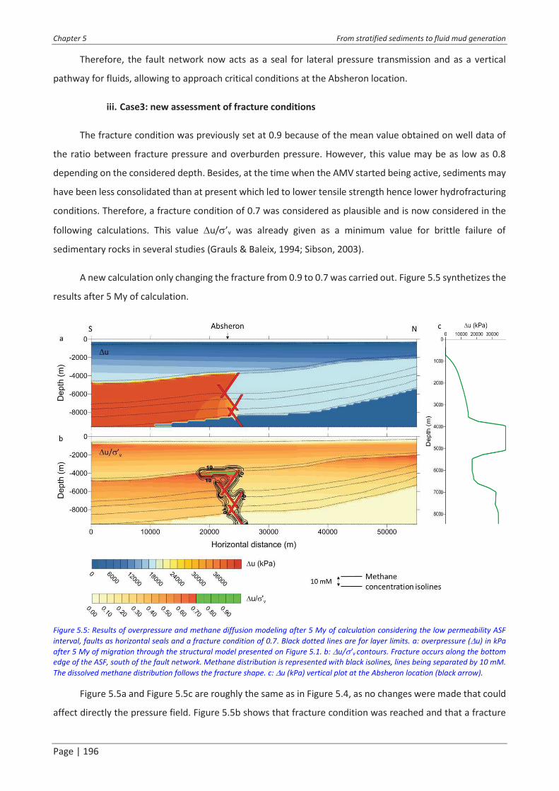
Chapter 5 From stratified sediments to fluid mud generation
Page | 196
Therefore, the fault network now acts as a seal for lateral pressure transmission and as a vertical
pathway for fluids, allowing to approach critical conditions at the Absheron location.
iii. Case3: new assessment of fracture conditions
The fracture condition was previously set at 0.9 because of the mean value obtained on well data of
the ratio between fracture pressure and overburden pressure. However, this value may be as low as 0.8
depending on the considered depth. Besides, at the time when the AMV started being active, sediments may
have been less consolidated than at present which led to lower tensile strength hence lower hydrofracturing
conditions. Therefore, a fracture condition of 0.7 was considered as plausible and is now considered in the
following calculations. This value Du/s�v was already given as a minimum value for brittle failure of
sedimentary rocks in several studies (Grauls & Baleix, 1994; Sibson, 2003).
A new calculation only changing the fracture from 0.9 to 0.7 was carried out. Figure 5.5 synthetizes the
results after 5 My of calculation.
Figure 5.5: Results of overpressure and methane diffusion modeling after 5 My of calculation considering the low permeability ASF
interval, faults as horizontal seals and a fracture condition of 0.7. Black dotted lines are for layer limits. a: overpressure (Du) in kPa
after 5 My of migration through the structural model presented on Figure 5.1. b: Du/s�v contours. Fracture occurs along the bottom
edge of the ASF, south of the fault network. Methane distribution is represented with black isolines, lines being separated by 10 mM.
The dissolved methane distribution follows the fracture shape. c: Du (kPa) vertical plot at the Absheron location (black arrow).
Figure 5.5a and Figure 5.5c are roughly the same as in Figure 5.4, as no changes were made that could
affect directly the pressure field. Figure 5.5b shows that fracture condition was reached and that a fracture
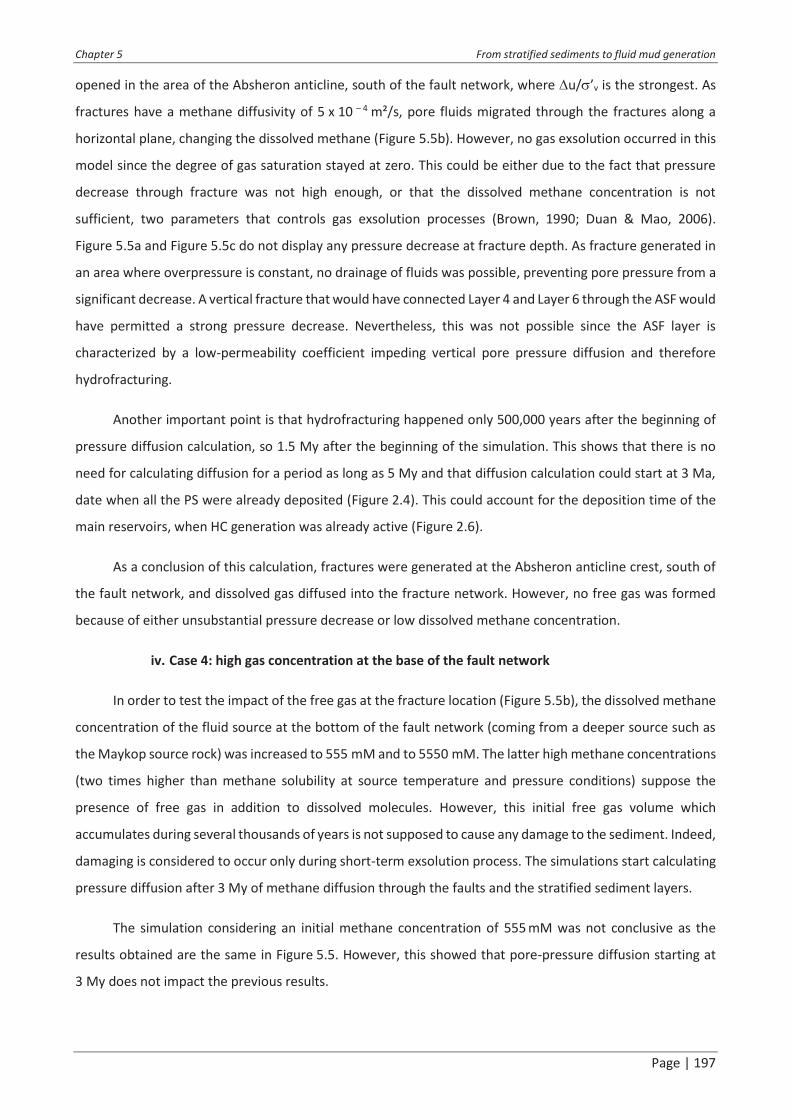
Chapter 5 From stratified sediments to fluid mud generation
Page | 197
opened in the area of the Absheron anticline, south of the fault network, where Du/s�v is the strongest. As
fractures have a methane diffusivity of 5 x 10 � 4 m²/s, pore fluids migrated through the fractures along a
horizontal plane, changing the dissolved methane (Figure 5.5b). However, no gas exsolution occurred in this
model since the degree of gas saturation stayed at zero. This could be either due to the fact that pressure
decrease through fracture was not high enough, or that the dissolved methane concentration is not
sufficient, two parameters that controls gas exsolution processes (Brown, 1990; Duan & Mao, 2006).
Figure 5.5a and Figure 5.5c do not display any pressure decrease at fracture depth. As fracture generated in
an area where overpressure is constant, no drainage of fluids was possible, preventing pore pressure from a
significant decrease. A vertical fracture that would have connected Layer 4 and Layer 6 through the ASF would
have permitted a strong pressure decrease. Nevertheless, this was not possible since the ASF layer is
characterized by a low-permeability coefficient impeding vertical pore pressure diffusion and therefore
hydrofracturing.
Another important point is that hydrofracturing happened only 500,000 years after the beginning of
pressure diffusion calculation, so 1.5 My after the beginning of the simulation. This shows that there is no
need for calculating diffusion for a period as long as 5 My and that diffusion calculation could start at 3 Ma,
date when all the PS were already deposited (Figure 2.4). This could account for the deposition time of the
main reservoirs, when HC generation was already active (Figure 2.6).
As a conclusion of this calculation, fractures were generated at the Absheron anticline crest, south of
the fault network, and dissolved gas diffused into the fracture network. However, no free gas was formed
because of either unsubstantial pressure decrease or low dissolved methane concentration.
iv. Case 4: high gas concentration at the base of the fault network
In order to test the impact of the free gas at the fracture location (Figure 5.5b), the dissolved methane
concentration of the fluid source at the bottom of the fault network (coming from a deeper source such as
the Maykop source rock) was increased to 555 mM and to 5550 mM. The latter high methane concentrations
(two times higher than methane solubility at source temperature and pressure conditions) suppose the
presence of free gas in addition to dissolved molecules. However, this initial free gas volume which
accumulates during several thousands of years is not supposed to cause any damage to the sediment. Indeed,
damaging is considered to occur only during short-term exsolution process. The simulations start calculating
pressure diffusion after 3 My of methane diffusion through the faults and the stratified sediment layers.
The simulation considering an initial methane concentration of 555 mM was not conclusive as the
results obtained are the same in Figure 5.5. However, this showed that pore-pressure diffusion starting at
3 My does not impact the previous results.

Chapter 5 From stratified sediments to fluid mud generation
Page | 198
Figure 5.6: Results of the simulation considering the ASF, sealing faults, a fracture condition of 0.7 and an initial methane
concentration of 5550 mM after 5 My. Black dotted lines are for layer limits. a: overpressure (Du) in kPa after 2 My of migration
through the structural model presented on Figure 5.1. b: Du/s�v contours. Fracture occurs along the bottom edge of the ASF, south of
the fault network. Methane distribution is represented with black isolines. The dissolved methane distribution follows the fracture
shape and is depleted around fractures due to gas exsolution. c: degree of gas saturation (Sg) calculated after fracture formation.
Values as high as 1 are reached in the central part of the fracture, in an area close to the fault network. d: preconsolidation pressure
(s�p). It increases linearly with depth, but it is disturbed in the same area where gas exsolution happened reaching zero in the center
of the fracture.
Figure 5.6 shows the results of the simulation with an initial methane concentration of 5550 mM.
Figure 5.6a shows that the overpressure field does not change compared to previous simulations. Figure 5.6b
shows a similar Du/s�v distribution than in Figure 5.6b with a fracture generation below the ASF, south of the
fault networks. The dissolved methane concentration follows the faults and fractures but with higher
concentrations, the lower value plotted being 500 mM (Figure 5.6b). Figure 5.6c displays the degree of free
gas saturation (Sg) calculated across the structural model. Sg is above zero in an area corresponding to the

Chapter 5 From stratified sediments to fluid mud generation
Page | 199
fractured area close to the fault network and just below the ASF limit. Maximum values of 1 are reached in
the center of the fractures. The model triggers gas exsolution locally after fracture generation for sufficient
dissolved methane concentration.
Gas exsolution has a twofold effect. First, dissolved methane distribution is disturbed and partly
depleted around the faults compared to the simulation proposed in Figure 5.5 (see Figure 5.6b) due to the
fact that, locally, a part of the initially dissolved methane exsolved to form free gas. Moreover, as the
simulation calculates the preconsolidation pressure (s�p), based on the equation in Figure 4.21 (Chapter
4:5.5) linking Sg with a preconsolidation ratio, we observe a local decrease in preconsolidation pressure in
response to the presence of free methane (Figure 5.6d). This decrease in s�p is observed in the area where Sg
is non-zero. s�p reaches almost 0 kPa where Sg is greater than 0.38, in areas where it was around 50 MPa
before gas exsolution (Figure 5.6d).
Thus, this simulation taking into account 1- the presence of ASF; 2- sealing faults; 3- a fracture condition
of 0.7; and 4- an initial methane concentration of 5550 mM, was able to model the sediment damage in an
area just below the ASF and at the Absheron anticline crest, through fracture opening and the subsequent
gas exsolution.
The integration of a low permeability layer corresponding to the ASF allowed transmitting
overpressure in the Upper Productive Series and reaching critical overpressure conditions. The modification
of fault hydraulic diffusivity in order to create horizontal seals resulted in critical conditions at the crest of
the Absheron Anticline. These critical conditions created fractures that, coupled with sufficiently high
dissolved methane concentration, allowed gas exsolution. Gas exsolution locally decreased the
preconsolidation pressure of sediments sufficiently for them to lose all their initial structure. The
observations made during the laboratory testing presented in Chapter 4 allow concluding that with the used
parameters, conditions for mud generation are reached in the Upper PS, at the AMV location.
3.2. Mud ascent
The approximate volume of mud and the initial geometrical conditions for the mud ascent modeling
were estimated from the previous calculations of the mud generation (Figure 5.6). The initial (2D) mud body
for all simulations was set as a convex-up half-disc with a radius of 500 m, its base (diameter of the half-disc)
being located 3400 meters below the seafloor with 500 meters of water column above and centered on the
horizontal direction (Table 5-2). For code1 v2, the initial mud overpressure was set at 35 MPa, which is the
pressure obtained in the mud generation zone at the end of the simulation presented in Figure 5.6. Mass-
densities used for all simulations are indicated in Table 5-2.

Chapter 5 From stratified sediments to fluid mud generation
Page | 200
Three values of the common viscosity of the ascending mud and host sediments were tested using
both codes (with and without pressurized mud) as well as the impact of the presence of vertical conduits and
of their length (Table 5-2).
Table 5-2: Parameters used in the different simulations completed during the study. The varying parameters are the sole sediment
viscosity and the fracture length.
code
version
viscosity
(kPa.s)
conduit
length (m)
dimensions mud source Mass-densities (kg/m3)
length depth dimension position overpressure bottom top mud Solid
grains
code1 v1
105
0
10 km
100 nodes
3900 m
100 nodes radius 500 m
x = 5000 m
z = 3900 m
No mud
overpressure
2100 1900 1900 2650
1000
2000
106
0
1000
2000
107
0
1000
2000
code1 v2
105
0
35 MPa
1000
2000
106
0
1000
2000
107
0
1000
2000
3.2.1. Code1 v1
Figure 5.7 displays the results of the simulation for the median case, µ = 10 6 kPa.s, using code1 v1. The
initial state shows the initial geometry of the mud generation zone modeled as a 500 meters radius half-disc.
The imposed mass-density is displayed, varying linearly from 1900 kg/m3 at the seafloor to 2100 kg/m3 at
3900 m. The mud mass-density is initially at 1900 kg/m3. The degree of gas saturation (Sg) is initially 0
everywhere except in the mud generation zone where it is set at 0.38. The gassy-mud column starts rising
after 3500 s. The changes in mass-density are mainly localized around the gassy-mud column and the velocity
vectors are mainly disturbed in the immediate vicinity of the mud source reaching 0.04 m/s at 3750 s. The
surrounding stratified sediments stay undisturbed, apart from the lateral edges where boundary conditions
create some artifacts. As the degree of gas saturation increases due to methane expansion, the mass-density
in the mud decreases (orange and green colors in Figure 5.8), triggering an acceleration of the process at
4500 s, when the gassy-mud column reaches 2200 m. The surrounding sediments are also impacted as the
gassy-mud column rises, as non-negligible displacements are computed 2000 m away from the column with
velocities reaching 0.1 m/s at 4500 s. The final stage (6000 s) shows that the gassy-mud column reaches the
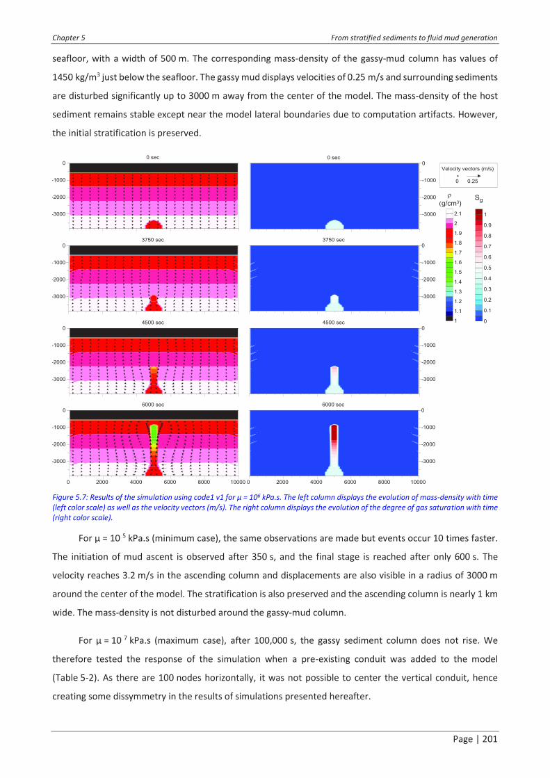
Chapter 5 From stratified sediments to fluid mud generation
Page | 201
seafloor, with a width of 500 m. The corresponding mass-density of the gassy-mud column has values of
1450 kg/m3 just below the seafloor. The gassy mud displays velocities of 0.25 m/s and surrounding sediments
are disturbed significantly up to 3000 m away from the center of the model. The mass-density of the host
sediment remains stable except near the model lateral boundaries due to computation artifacts. However,
the initial stratification is preserved.
Figure 5.7: Results of the simulation using code1 v1 for µ = 106 kPa.s. The left column displays the evolution of mass-density with time
(left color scale) as well as the velocity vectors (m/s). The right column displays the evolution of the degree of gas saturation with time
(right color scale).
For µ = 10 5 kPa.s (minimum case), the same observations are made but events occur 10 times faster.
The initiation of mud ascent is observed after 350 s, and the final stage is reached after only 600 s. The
velocity reaches 3.2 m/s in the ascending column and displacements are also visible in a radius of 3000 m
around the center of the model. The stratification is also preserved and the ascending column is nearly 1 km
wide. The mass-density is not disturbed around the gassy-mud column.
For µ = 10 7 kPa.s (maximum case), after 100,000 s, the gassy sediment column does not rise. We
therefore tested the response of the simulation when a pre-existing conduit was added to the model
(Table 5-2). As there are 100 nodes horizontally, it was not possible to center the vertical conduit, hence
creating some dissymmetry in the results of simulations presented hereafter.

Chapter 5 From stratified sediments to fluid mud generation
Page | 202
Two conduit lengths were tested: 1000 m and 2000 m from the base of the model (Table 5-2). The
result of the simulation with µ = 10 5 kPa.s and a 1000 m long vertical conduit is presented in Figure 5.8,
where the conduit is displayed at the initial stage, with the same mass-density and the same degree of gas
saturation as the mud generation zone. The initiation of gassy-mud ascent starts at 300 s. The gassy-mud
ascent is mainly focused along the conduit, but it is superimposed with the normal gassy-mud ascent due to
the presence of the mud source (as was observed without conduit). It is particularly visible as the conduit is
not perfectly centered over the mud generation zone. The final stage is reached at 750 s. The final width of
the gassy-mud column is 250 m. The velocity of the host sediments reaches 1.2 m/s at the direct proximity
of the conduit and decreases to nil over a distance of 3 km. The timing of ascent conduit of 2-km conduit is
very similar to the previous one, but the velocity only reaches 0.5 m/s, and the gassy-mud ascent is only
focused above the vertical discontinuity, hence the final gassy-mud column is only 100 m wide.
Figure 5.8: Results of the simulation using code1 v1 for µ = 105 kPa.s and a 1000 m long vertical conduit. The left column displays the
evolution of mass-density with time (left color scale) as well as the velocity vectors (m/s). The right column displays the evolution of
the degree of gas saturation with time (right color scale).
We also tested the impact of conduits for µ = 10 6 kPa.s. The results are overall similar to what has
been described above with µ = 10 5 kPa.s, apart from the timing: initiation of gassy-mud ascent happens after
3000 s for both conduit lengths, and mud reaches the seafloor after 7000-7500 s. The maximum velocity is

Chapter 5 From stratified sediments to fluid mud generation
Page | 203
0.12 m/s for a 1-km conduit and 0.05 m/s for a 2-km conduit conduit. The width of the gassy-mud column
remains unchanged.
With µ = 10 7 kPa.s, even with 2 km-long conduits, no gassy-mud column was observed, even after
100,000 s, corresponding to over 3 weeks of computation time, exceeding the time limitation imposed on
the Datarmor supercomputer.
3.2.2. Code1 v2
Code1 v2 considers the initial mud overpressure and its evolution with gas expansion. Fluid pressure
in Eq. (11) (Chapter 2:3.4.4) is calculated separately through Boyle�s law when free gas is present.
Figure 5.9: Results of the simulation using code1 v2 for µ = 106 kPa.s. The left column displays the evolution of mass-density with time
(left color scale) as well as the velocity vectors (m/s). The right column displays the evolution of the degree of gas saturation with time
(right color scale).
Figure 5.9 displays the results of the simulation for µ = 10 6 kPa.s using code1 v2. The initial state is the
same as in Figure 5.7. The different stages described for code1 v1 are the same with this version, but they
occur earlier in the simulation. The ascending column initiates at 1750 s, and it is accompanied by a slight
disruption in velocity vectors as shown in Figure 5.9 at 2000 s. This disruption increases as the ascending
gassy-mud column rises, reaching 0.35 m/s in the ascending column at the final stage of the simulation and
affecting a radius of 3000 m around the center of the model. The ascending column reaches the seafloor
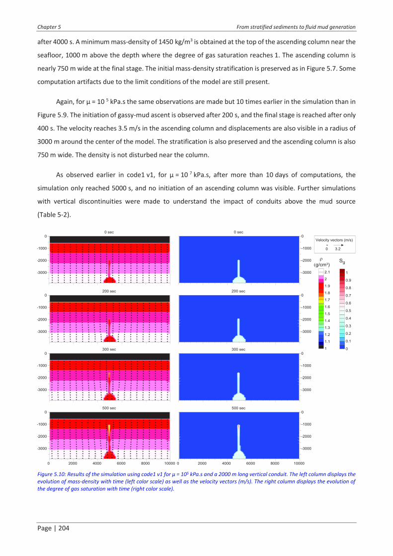
Chapter 5 From stratified sediments to fluid mud generation
Page | 204
after 4000 s. A minimum mass-density of 1450 kg/m3 is obtained at the top of the ascending column near the
seafloor, 1000 m above the depth where the degree of gas saturation reaches 1. The ascending column is
nearly 750 m wide at the final stage. The initial mass-density stratification is preserved as in Figure 5.7. Some
computation artifacts due to the limit conditions of the model are still present.
Again, for µ = 10 5 kPa.s the same observations are made but 10 times earlier in the simulation than in
Figure 5.9. The initiation of gassy-mud ascent is observed after 200 s, and the final stage is reached after only
400 s. The velocity reaches 3.5 m/s in the ascending column and displacements are also visible in a radius of
3000 m around the center of the model. The stratification is also preserved and the ascending column is also
750 m wide. The density is not disturbed near the column.
As observed earlier in code1 v1, for µ = 10 7 kPa.s, after more than 10 days of computations, the
simulation only reached 5000 s, and no initiation of an ascending column was visible. Further simulations
with vertical discontinuities were made to understand the impact of conduits above the mud source
(Table 5-2).
Figure 5.10: Results of the simulation using code1 v1 for µ = 105 kPa.s and a 2000 m long vertical conduit. The left column displays the
evolution of mass-density with time (left color scale) as well as the velocity vectors (m/s). The right column displays the evolution of
the degree of gas saturation with time (right color scale).

Chapter 5 From stratified sediments to fluid mud generation
Page | 205
At µ = 10 5 kPa.s, the presence of a 1 km long vertical discontinuity generates similar effects to those
obtained with code1 v1 and displayed in Figure 5.8. The gassy-mud column initiates at 200 s, mainly focusing
along the conduit, but the direct impact of the mud generation zone is also visible (same as Figure 5.8). The
column reaches the seafloor after 400 s, reaching 750 m in diameter and velocities of 4.2 m/s above the mud
chamber. The velocity field is disturbed in a radius of 3 km around the conduit. The case of a 2-km conduit is
displayed in Figure 5.10. An ascending gassy-mud column starts forming at 200 s just at the termination of
the vertical conduit. The mud column gets larger at 300 s, forming a drop-shaped low density area. The gassy
mud reaches the surface between 500 and 600 s with velocities reaching locally 3.2 m/s at the intersection
between the conduit and the mud chamber. The gassy-mud column is 100 m wide at the end of the
simulation.
This version of the code leads to computation times even longer than the v1, so no process initiation
was observed for µ = 10 7 kPa.s, even with 2 km-long conduits.
Table 5-3: Synthesis of the main results obtained from the different simulations computed in this study. The initiation time of gassy-
mud ascent, the time needed to reach the seafloor, the maximum velocity and the final diameter of the gassy-mud column are
displayed for the two code versions.
code µ (kPa.s) Conduit
length (m) Initiation (s) Extrusion (s)
Max. velocity
(m/s) Final diameter of gassy-
mud column (m)
1 v1
105 0 350 600 3.2 1000
1000 300 750 1.2 250 2000 300 750 0.5 100
106 0 3500 6000 0.25 500
1000 3000 7000 0.12 250 2000 3000 7500 0.05 100
107 0
Computation too time consuming 1000 2000
1 v2
105 0 200 400 3.5 750
1000 200 500 4.2 400 2000 200 500 3.2 100
106 0 1750 4000 0.35 750
1000 1500 4500 0.36 400 2000 2000 4750 0.32 100
107 0
Computation too time consuming 1000 2000
All the results obtained with the different 2D simulations discussed above are synthesized in Table 5-3.
These results highly depend on the spatial and temporal resolution of the simulations, hence small variations
are not considered to be relevant. It clearly shows that when viscosity increases by one order of magnitude,
velocity decreases by one order of magnitude while the timing of initiation and extrusion increases by one
order of magnitude (Table 5-3). When mud overpressure is considered in the simulations, it decreases the

Chapter 5 From stratified sediments to fluid mud generation
Page | 206
time for initiation and extrusion by a ratio of 0.65 to 0.5 (Table 5-3). The presence of vertical conduits above
the mud chamber mainly influences the Vmax which seems to decrease as the length of the conduit increases
in the case of code1 v1 (Table 5-3). For code1 v2, Vmax seems to remain roughly constant. The presence of a
conduit also influences the final diameter of the gassy-mud column that decreases as the length of the
conduit increases (Table 5-3).
3.2.3. Extrapolation to realistic viscosities: 1D calculations
In order to extrapolate the 2D simulation results obtained through the code modified from
Tryggvason (2012), we tested simple 1D calculations based on the case of a buoyant magma flow along a
vertical dyke (Furbish, 1997) in order to compare the velocities and timing obtained. Using Eq. (17) with r the
radius of the mud chamber (r = 500 m) and taking x = 0 (maximum velocity above the center of the mud
chamber) it was possible to obtain the maximum velocity above the mud chamber for varying viscosities.
Figure 5.11a shows the results of 1D calculations of maximum velocities (Vmax) for viscosities comprised
between 10 5 and 10 12 kPa.s, considered as a valid approximation range for mud viscosities that are typically
below the viscosity of sedimentary rocks. Two sets of models were run: the first one without initial mud
overpressure (black), corresponding to the mud mass-density calculated through Eq. (13); the second (red
line) considers an initial mud overpressure. Overpressure is limited to 78% of the effective stress (value of
Du/s�v near the mud source at the end of 2D diffusion models, see Chapter 5:3.1.2.iv), thus, the mass-density
of mud was multiplied by 0.78 to take the mud overpressure into account. The maximum velocities obtained
above the mud chambers for the 2D simulations without conduit are also plotted in Figure 5.11a.
Figure 5.11b displays the same results in terms of minimum time for extrusion that was calculated
considering that the velocity is Vmax all along the conduit. The results in Figure 5.11b clearly show that the
minimum time needed for the buoyant mud to reach the seafloor and form a mud volcano depends on mud
viscosity.
The 1D calculations shows that the maximum velocity is inversely proportional to the vioscosity
(Figure 5.11a). Considering the initial mud overpressure, without modifying the viscosity, increases Vmax by a
factor 4.5, so that the two trends are parallel. For higher viscosities (10 12 kPa.s), the maximum velocity is
comprised between 10 � 6 and 10 � 7 m/s. Logically, the time for extrusion increases by an order of magnitude
for each order of magnitude of µ (Figure 5.11b), results directly arising from the form of Eq. (17). The
consideration of the mud overpressure allows reducing this time for extrusion. Therefore, for µ = 10 12 kPa.s,
it would take a minimum of 500 years for the buoyant mud to reach the surface if the mud overpressure is
not considered, while it would take only 100 years if the mud overpressure is integrated in the calculation.

Chapter 5 From stratified sediments to fluid mud generation
Page | 207
Figure 5.11: Results of 1D calculations based on the case of a buoyant magma flow along a vertical dyke presented in Furbish (1997)
considering a radius of 500 m corresponding to the mud source radius, compared to results obtained with 2D simulations. a: maximum
velocity versus viscosity, b: minimum time for extrusion versus viscosity. Black lines with crosses correspond to the case where the
initial mud overpressure is not considered, red lines are for the case with mud overpressure. Grey dots correspond to the results of the
2D simulations using code1 v1 and white dots the results of 2D simulations with code1 v2.
The 2D simulations results display the same relationship. µ and Vmax are inversely proportional
(Figure 5.11a). Taking into account the initial mud overpressure in code1 v2 leads to a 4-fold increase of Vmax
compared with code1 v1 (Figure 5.11a). Moreover, the values obtained with code1 v1 stands close to the
black line (1D calculations without mud overpressure), and the values of code1 v2 are closer to the red line
compared to code1 v1 results (1D calculations considering mud overpressure).
The same calculation was applied but in the case of a 50 m wide conduit corresponding to the size of
the conduits in the2D simulations (Figure 5.12). The same relationship between µ and Vmax and µ and the
time for extrusion are displayed in Figure 5.12. The impact of mud overpressure seems to be limited as the
difference between the Vmax and the time for extrusion obtained considering mud overpressure and without
mud overpressure is reduced compared to Figure 5.11. Moreover, the Vmax extracted from 2D simulations
are larger by nearly one order of magnitude than those obtained from 1D calculations (Figure 5.12a).
Therefore, the time for extrusion are smaller by one order of magnitude (Figure 5.12b). Besides, the conduit
width corresponds to the minimum that could be computed considering the model resolution, 1 node
corresponding to 100 m and the conduit being computed over a unique node. Hence, the results displayed
are not relevant of the circulation that would occur in natural fractures whose width is much smaller.
From this 1D calculation, it arises that the time required for achieving extrusion, considering a viscosity
of 10 12 kPa.s, is significantly increased. Considering mud overpressure, it would take more than 10,000 years
for the mud to reach the surface through thin fractures when it was 100 years for the calculation considering
the mud chamber radius.

Chapter 5 From stratified sediments to fluid mud generation
Page | 208
Figure 5.12: Results of 1D calculations based on the case of a buoyant magma flow along a vertical dyke presented in Furbish (1997)
considering a radius of 50 m corresponding to the conduit width, compared to results obtained with 2D simulations. a: maximum
velocity versus viscosity, b: time for extrusion versus viscosity. Black lines with crosses correspond to the case where the initial mud
overpressure is not considered, red lines are for the case with mud overpressure. Grey dots correspond to the results of the 2D
simulations using code1 v1 and white dots the results of 2D simulations with code1 v2.
4. Discussion
4.1. Synthesis of the main results
The consideration of the low-permeability Anhydritic Surakhany Formation (ASF) allowed to simulate
in 1D the generation of a sedimentation-related overpressure contrast between layer 6 and deeper layers
reproducing the overpressure sharp increase observed in well-log data (Figure 3.14A). Moreover, the model
simulates maximum overpressure values of 40 MPa corresponding to the values measured in situ at the
Absheron exploration wells (Figure 3.14A). It also improved the 2D diffusion model presented in Chapter
3:4.4.2 (Figure 3.17) with overpressure now occurring essentially below the ASF and transmitted through
Layer 4 (Figure 5.3). Overpressure diffusion started after 3 My of simulation, a date corresponding to the
deposition of the entire Productive Series interval. Lateral compartmentalization of the 2D model through
the presence of faults having low horizontal permeability (Gautherot et al., 2015; Javanshir et al., 2015) was
necessary to create overpressured conditions at the location of the AMV (Figure 5.4). Faults are often
regarded as presenting permeability anisotropy depending on their internal structure and material and
depending on external parameters such as pore pressure (Caine et al., 1996; Evans et al., 1997; Schneider et
al., 2004; Wibberley et al., 2008; Deville et al., 2010; Morley et al., 2017; Henry et al., 2019), thus methane-
saturated water migration from the Maykop Fm. was provided by high methane diffusivity in faults, artificially
simulating high vertical permeability accounting for advection processes. A new fracture condition of 0.7 was
adopted, based on pressure logs at well sites, allowing to create a fractured area at the Absheron crest, just
below the ASF (Figure 5.5). For an initial methane concentration of 5550 mM, gas exsolution was triggered
in the fractured area resulting in a strong sediment damage in the fracture zone, with preconsolidation

Chapter 5 From stratified sediments to fluid mud generation
Page | 209
pressure locally approaching zero (Figure 5.6). From the results of the laboratory testing discussed in
Chapter 4, the improved 2D diffusion model simulated the mud generation zone formation below the
Absheron MV.
To understand a possible ascent mechanism of the mud from its source to the seafloor, we based our
approach on fluid mechanics using modified 2D Navier-Stokes equations considering the impact of gas
expansion (Boyle�s law) on the mass-density of the mud. Mud viscosities were limited to values between
10 5 kPa.s and 10 7 kPa.s because higher viscosities resulted in exceedingly long simulations and results were
extrapolated with a simple 1D calculation to viscosities up to 10 12 kPa.s. Results of the 2D simulations show
that ascent velocity is inversely proportional to mud viscosity, while the times needed for mud ascent
initiation and for mud extrusion is proportional to viscosity (Table 5-3). When mud overpressure is considered
in the simulations, it decreases the time for initiation and extrusion by a ratio of 0.5-0.65 (Table 5-3). The
presence of conduits mainly influences the final width of the gassy-mud column, which decreases with an
increasing conduit length (Table 5-3). Through one-dimensional extrapolation it would take a minimum of
500 years for a buoyant high-viscosity mud to reach the surface if mud overpressure is not considered, while
it would take only 100 years if the mud overpressure is integrated in the calculation (Figure 5.11b).
Considering the radius of a conduit (Figure 5.12b), it arises that the timing for extrusion is significantly
increased as it would take more than 10,000 years for the same overpressured mud to reach the surface.
Combining 1D and 2D simulations, adapting the Navier-Stokes equations to consider the impact of gas
expansion on sediment mass-density through Boyle�s law and the influence of mud overpressure over the
ascension velocity allowed estimating the time needed for mud generated at depth to reach the seafloor and
to form a mud volcano through density-inversion.
In the following, the results of the calculations carried out in this chapter will be discussed and
confronted to previous research to assess the two main questions of the introduction:
· Is it possible to simulate mud generation conditions at depth by considering the mechanical
properties of sediments, the sedimentation rates, structural elements and the impact of gas
exsolution?
· Is the sole impact of gas expansion on the mud properties able to drive mud up to the seafloor?
4.2. Overpressure, hydrofracturing and gas exsolution: from stratified
sediments to fluid mud
Calculations of pressure related to the maximum gas column that could have been trapped within the
ASF in Chapter 3 showed that the sole effect of the presence of a gas reservoir at the crestal location of the
Absheron fold cannot explain the formation of the Absheron mud volcano, as the fracture pressure was not
reached. Hydrofracturing is believed to be necessary to initiate a MV formation as demonstrated through the
monitoring of the Lusi initiation (Tingay et al., 2017) and through the analysis of the Absheron Mud Volcano

Chapter 5 From stratified sediments to fluid mud generation
Page | 210
dataset (Chapter 3). Therefore, additional parameters are required to explain the AMV formation. The
sedimentation rates recorded in the SCB are among the highest in foreland basins (Tagiyev et al., 1997; Allen
et al., 2002; Smith-Rouch, 2006; Egan et al., 2009; Green et al., 2009). High sedimentation generates
overpressure in low-permeability strata (Osborne & Swarbrick, 1997; Dugan & Flemings, 2000; Opara, 2011)
and overpressure is one of the key triggers and drivers for MV formation (Dimitrov, 2002; Kopf, 2002;
Deville, 2009; Mazzini & Etiope, 2017).
The 2-D diffusion model presented in this chapter is based on regional data extracted from literature
(Diaconescu et al., 2001; Green et al., 2009), on observations and in situ measurements made on the
Absheron gas condensate field, as well as on the laboratory experiments presented in Chapter 4. The
regional-scale pressure gradient and northward fluid circulation from the deep SCB was already observed
and discussed by several studies (Bredehoeft et al., 1988; Gautherot et al., 2015; Javanshir et al., 2015), and
this type of modeling, studying the influence of regional physical parameters such as sedimentation rate and
pressure gradient on local structures such as landslides or venting sites, was already applied to other
sedimentary basins (Dugan & Flemings, 2000; Schneider et al., 2004; Kvalstad et al., 2005; Hustoft et
al., 2009). Deville et al. (2010) applied a similar fluid flow numerical model to show that MVs in Trinidad are
located above overpressured areas. However, it is the first time, in our knowledge, that a 2D-diffusion model
is applied to simulate sediment remobilization into mud at depth.
More precise measurements and estimations of layer permeability and fracture pressure would now
be needed to improve this simulation. Laboratory testing on rock fragments from the different modeled
layers would be necessary to improve their hydro-mechanical properties. Most of the modeled stratigraphic
intervals are known to outcrop onshore, along the Kura Basin, the Absheron Peninsula or in the Greater
Caucasus where such rock samples would be easily accessible (Morton et al., 2003; Hinds et al., 2004; Vincent
et al., 2010; Bochud, 2011; Choi et al., 2011; Forte et al., 2015; Abdullayev & Leroy, 2016). Fracturing pressure
was only estimated from pressure logs. However, LOT/FIT data shown in Figure 3.14A indicate that
hydrofracturing may occur for an overpressure of 25 MPa. Therefore, less than 2 My of overpressure diffusion
may be necessary in our simulation in order to obtain the needed 25 MPa to trigger fracture generation as
the fracture in Figure 5.6 generated for over 35 MPa of overpressure.
The simulation generated a horizontal fractured area where gas was able to exsolve, reaching Sg
greater than 0.38 locally and therefore damaging sediments that entirely lost their preconsolidation pressure.
This area represents the mud generation zone and is 1300 m long and locally 220 m thick (Figure 5.6). The
presence of the low-permeability ASF prevented pore pressure and therefore fractures to propagate
vertically even if the maximum principal stress is vertical, the simulation ignoring the impact of compressive
tectonics that are observed over the basin.

Chapter 5 From stratified sediments to fluid mud generation
Page | 211
The 2D modeling presented in this study allows drawing a coupled process for mud generation below
the AMV. Due to high sedimentation rates, overpressure is generated in the deeper part of the SCB and is
transmitted northwards along under-compacted layers that kept an abnormally high permeability. The fault
system at the core of the Absheron anticline leads to local overpressure build-up above the crest of the
anticline, eventually initiating hydrofracturing and saturating the pore waters of the Upper Productive Series
with methane. Hydrofracturing may trigger a local decrease in overpressure, allowing exsolution of the
dissolved methane and triggering sediment damage when Sg exceeds 0.38 (see Chapter 4). Thus, the 2D
diffusion model integrating the mechanical properties of sediments, sedimentation rates,
compartmentalization effect of faults and regional seal and the impact of gas exsolution is able to reproduce
the mud generation conditions at depth below the AMV.
4.3. Mud extrusion resulting from density-inversion driven by gas
exsolution
Once the mud is generated at depth, it is necessary to understand how it is transported to the surface.
The modeling work shows that mud ascent time is proportional to mud viscosity. Taking mud overpressure
into account improve the convergence of 1D and 2D results (Figure 5.11). Similar values of velocity were
obtained by Collignon et al. (2018b) who calculated flow rates depending on pipe radius, particle size and
density and the type of gas for equivalent viscosities. One-dimensional extrapolation allows to test viscosities
closer to those of sedimentary rocks, which was not possible on the 2D simulations due to time limitations.
It would take approximately 100 years for the mud generated at the AMV location to rise to the surface if
mud was only transported through density inversion and mud overpressure. The link between 2D results and
the extrapolation in 1D may not straight forward. The extrapolation in 1D is made over 6 orders of magnitude
of viscosities and compared to only two 2D control points. The relationship between mud remobilization and
the host sediment viscosity may not be a linear process when dealing with high values of µ. Therefore, the
results have to be addressed with precautions. Nevertheless, some MVs display very small extrusion rates,
such as the Koturdag (onshore Azerbaijan), that extrudes high viscosity and slightly wet mud with an
estimated rate of 0.02 m/day (Dupuis, 2017), in other words 2.3 x 10 � 7 m/s, which is the order of magnitude
obtained from our modeling.
The presence of a preexisting conduit in our simulations does modifies the extrusion time, but it
reduces the extrusion rate as a smaller volume of mud is able to rise through the sedimentary column. One-
dimensional calculations considering fracture radius show that for µ = 10 12 kPa.s, the extrusion time is close
to 10,000 years. The simulations shown here do not address multi-phase flow, gas being only considered in
the mass-density calculation. If free-gas was able to flow directly through the fracture, it may be able to
fracture and/or damage shallower sediments, forming a secondary mud generation zone. This was observed
at Lusi location, where the BJP-1 well allowed overpressured fluids charged with gas to flow to shallower and
more fragile strata, triggering hydrofractures and mud generation (Tingay et al., 2008, 2015).
Chapter 5 From stratified sediments to fluid mud generation
Page | 212
In contrast to our numerical model in which mud ascent occurs along a unique wide fracture, field
work reported by Roberts et al. (2010) has shown that mud volcano conduits rather consist of an intricate
and complex fractured volume with detached and rotated blocks that was observed on field by Roberts et
al. (2010). They explain their observations by the rising of overpressured and low-density mud that generates
and propagates fractures as it rises, slowly opening its way up to the surface. Thus, the 2D simulations should
rather compute the progressive opening of fractures as mud overpressure increases due to gas expansion.
This would imply a combination of solid-rock mechanics and fluid mechanics that represents a complete field
of research in modeling and computation, notably applied to hydrofracturing issues in well bores (Mainguy
& Longuemare, 2002; Wu & Olson, 2015). The Lusi catastrophe allowed to monitor the initiation of a mud
volcano formation. From the analysis of drilling reports, and notably records on the expelled gas, drilling mud
losses and drilling mud pressure, Tingay et al. (2017) show that 24-48 hours separate the moment when free-
gas was detected at the bottom of the well, and the moment when the mud extruded at the surface.
Therefore, gas-driven mud generation and transport seem to occur very fast. Our model points to a transport
duration of 100 years to cross the 3000 meters of strata separating the mud source from the surface but
through the sole density inversion driven by gas expansion. The impact of gas expansion on overpressure and
on rock failure is not explored but is expected to reduce significantly the time for extrusion. Besides, this
combination of processes would imply a similar plumbing system as the one described by Roberts et
al. (2010).
Another limitation of the current model is that the influence of gas exsolution on mud rheology was
not accounted for. The presence of gas and liquids in the mud are known to strongly affect its viscosity
(Kopf, 2002; Mazzini & Etiope, 2017). Collignon et al. (2018b) and Zoporowski & Miller (2009) have both
considered a dynamic viscosity in their simulations and shows that the contrast between mud viscosity and
the viscosity of the surrounding rock increases flow rates. Modeling results of Collignon et al. (2018b)
demonstrated that the feeding pipe of the Lusi MV has to be smaller than 1.5 m radius in order to match its
maximal mud discharge, when our model displays very long extrusion time for small fractures. Thus, the
integration of a dynamic viscosity depending on gas content, would certainly increases the velocity of the
extrusion process in our model. It will also allow to study the effect of low-viscosity layers, for instance
containing evaporites like the ASF. Besides, the gas mass-density was considered negligible in the calculation
of the mud mass-density. However, gas mass-density highly depends on the pressure and temperature
conditions, and represents 1/5 of the water mass-density at 35 MPa and 50 °C.
Finally, the code of Tryggvason (2012) was developed to answer fluid mechanics issues. Working with
values corresponding to a geological background leads to very long calculation time due to computing
limitations arising from the resolution method. Therefore, the code should be improved or another
resolution method should be explored in order to be able to run 2D simulations with parameters fitting the
geological reality over shorter period of time.

Chapter 5 From stratified sediments to fluid mud generation
Page | 213
The sole effect of gas expansion on the mud mass-density is thus able to drive mud ascent up to the
seafloor. The process may be accelerated if the influence of gas exsolution and expansion on mud viscosity
and on fracture propagation ahead of the rising mud. This modeling work resulted in extrusion rates of the
same order of magnitude that what is measured on MVs extruding high viscosity mud.
4.4. Towards a quantitative formation model for the Absheron mud
volcano
The conceptual formation model developed in Chapter 3 for the AMV was improved by integrating the
main findings of Chapter 4 and of the numerical models. This allows to move from a purely qualitative model,
to a semi-quantitative one including the formation dynamics as a function of the main physical parameters
controlling the mud volcano formation: ratio of overpressure to vertical effective stress, dissolved methane
concentration and degree of gas saturation. The updated formation model is composed of 7 different phases
shown in the different panels of Figure 5.13:
Stage 1 - At 3.4 Ma, end of the rapid deposition of the Productive Series (over 3.5 km in 2 Ma) above
the gas-mature Maykop Formation that generated hydrocarbons diffusing slowly through the sedimentary
column (Figure 5.13a). The Maykop Formation started generating gas during the Late Miocene in the Shah
Deniz region located less than 50 km away from the Absheron gas discovery (Figure 2.9 in Alizadeh et
al., 2017). Moreover, the deposition of the Anhydritic Surakhany Formation provided an efficient seal
allowing a slow and uniform overpressure build-up in the Productive Series generated by high sedimentation
rates.
Phase 2 � At 0.7 Ma, the growth of the rate of deformation at the Absheron fold increased significantly.
Methane circulation was therefore focused into the faulted core of the anticline (Figure 5.13b). The
difference of overburden between the anticline and adjacent syncline generated an overpressure gradient
allowing overpressure build-up against the sealing faults (Figure 5.13b). Besides, at the anticline crest, the
vertical effective stress s�v is lower than on the flanks due to reduced overburden thickness. Thus,
overpressure generation and transmission as well as low s�v at the crest increased the Du /s�v ratio.
Phase 3 �At # 0.6 Ma, Du /s�v ratio reached the hydro-fracturing threshold of 0.7 (Figure 5.13c),
allowing hydrofracturing. These led to a local decrease of overpressure through fluid dissipation and
triggered methane exsolution where the dissolved-methane concentration reached the methane solubility
(Henry�s law; Figure 5.13c). For a degree of gas saturation higher than 0.38, the sediment lost its
preconsolidation pressure leading to mud generation (Figure 5.13c).
Phase 4 � The presence of gas bubbles in the mud significantly reduced its mass-density and its viscosity
(Figure 5.13d). Therefore, the gassy mud started to rise along the open fractures. As the gas bubbles moved
up, they expanded (following Boyles�s law), hence increasing the degree of gas saturation and decreasing the
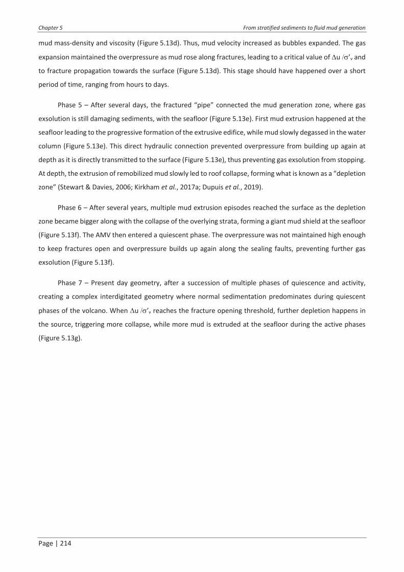
Chapter 5 From stratified sediments to fluid mud generation
Page | 214
mud mass-density and viscosity (Figure 5.13d). Thus, mud velocity increased as bubbles expanded. The gas
expansion maintained the overpressure as mud rose along fractures, leading to a critical value of Du /s�v and
to fracture propagation towards the surface (Figure 5.13d). This stage should have happened over a short
period of time, ranging from hours to days.
Phase 5 � After several days, the fractured �pipe� connected the mud generation zone, where gas
exsolution is still damaging sediments, with the seafloor (Figure 5.13e). First mud extrusion happened at the
seafloor leading to the progressive formation of the extrusive edifice, while mud slowly degassed in the water
column (Figure 5.13e). This direct hydraulic connection prevented overpressure from building up again at
depth as it is directly transmitted to the surface (Figure 5.13e), thus preventing gas exsolution from stopping.
At depth, the extrusion of remobilized mud slowly led to roof collapse, forming what is known as a �depletion
zone� (Stewart & Davies, 2006; Kirkham et al., 2017a; Dupuis et al., 2019).
Phase 6 � After several years, multiple mud extrusion episodes reached the surface as the depletion
zone became bigger along with the collapse of the overlying strata, forming a giant mud shield at the seafloor
(Figure 5.13f). The AMV then entered a quiescent phase. The overpressure was not maintained high enough
to keep fractures open and overpressure builds up again along the sealing faults, preventing further gas
exsolution (Figure 5.13f).
Phase 7 � Present day geometry, after a succession of multiple phases of quiescence and activity,
creating a complex interdigitated geometry where normal sedimentation predominates during quiescent
phases of the volcano. When Du /s�v reaches the fracture opening threshold, further depletion happens in
the source, triggering more collapse, while more mud is extruded at the seafloor during the active phases
(Figure 5.13g).

Chapter 5 From stratified sediments to fluid mud generation
Page | 215

Chapter 5 From stratified sediments to fluid mud generation
Page | 216
Chapter 5 From stratified sediments to fluid mud generation
Page | 217

Chapter 5 From stratified sediments to fluid mud generation
Page | 218
Figure 5.13: Formation model for the Absheron mud volcano based on in situ observations and measurements, sediment analysis,
laboratory testing and mud generation and remobilization numerical modeling. Details of the different stages displayed in a, b, c, d,
e, f and g are in the text. h: legend corresponding to a, b, c, e, f, g.

Chapter 5 From stratified sediments to fluid mud generation
Page | 219
5. Conclusion
This chapter explored the possibility of simulating mud generation and extrusion processes through
numerical modeling based on simple physical principles. The ultimate goal is to simulate the complete
formation of the Absheron Mud Volcano (AMV) and to quantify the overpressure conditions and methane
concentration that led to the present structure. A first model, considering 2D-diffusion laws (Darcy�s law and
Fick�s law) was used to explain the location of the AMV as well as the conditions required to generate fluid
mud from stratified solid sediments. The second model applies a fluid mechanics approach to test whether
the sole impact of gas expansion on the mud density can lead to mud extrusion. The main results are:
1- The 2D-diffusion model showed that using sedimentation rates corrected from compaction to
calculate overpressure in the deep basin and considering the low-permeability Anhydritic
Surakhany Formation and sealing faults as flow baffles, critical fracture conditions are obtained
at the crest of the Absheron anticline, below the ASF, where the depleted area was observed
in Chapter 3.
2- A methane concentration of 5550 mM, injected at the base of the fault network considered as
permeable in the vertical direction creates the conditions for triggering gas exsolution and
subsequent loss in preconsolidation pressure showing that liquid mud is generated at depth.
3- Mud ascent up to the seafloor through the sole density-inversion provoked by gas expansion
is possible over a period of 100 years minimum. This period of time for extrusion corresponds
to extrusion rates measured at particular MVs.
4- To accelerate the process, additional parameters such as dynamic viscosity and the upward
propagation of fracture as consequences of gas expansion have to be considered.
We show that simple physical models integrating realistic geological and hydro-mechanical parameters
and behavior of sediments are able to reproduce the conditions that initiated the formation of the Absheron
Mud Volcano. We simulated the key processes inferred from the available dense dataset and from the
present geometry that were described in the conceptual model in Chapter 3. A dense and high-quality
dataset is paramount to complete such models using the same methodology on other mud volcanoes located
in similar contexts.

Chapter 5 From stratified sediments to fluid mud generation
Page | 220

Page | 221
Chapter 6: Synthesis, conclusions and perspectives
Abstract
The dataset composed of geophysical data (seismic, bathymetry), in situ measurements and sediment
cores, allowed to show that the Anhydritic Surakhany Formation and some other Upper Productive Series
intervals are the source for the Absheron Mud Volcano. The study of pressure data and a preliminary
numerical model proved that overpressure initiated by the regional high sedimentation rates associated to
gas circulating along the fault system coring Absheron, would explain its formation. Experimental testing
study using a new consolidation apparatus to saturate samples with carbonated water and to create free gas
by decompression demonstrated the capacity of gas exsolution to transform compacted sediments into mud
for a critical degree of gas saturation. Numerical models using simple physical diffusion equations and
integrating results from observations, in situ measurements and laboratory testing results were able to
reproduce the mud generation process at the Absheron location. Finally, fluid mechanics models show that
mud extrusion through density inversion is possible.
Possible improvements to the developed methods have been identified. The dataset that could be
improved through new processing and further analysis. The consolidation apparatus could be upgraded to
support higher pressures and better simulate real geological stress conditions. Numerical models, notably
the fluid mechanics approach, could be made more realistic, for instance by integrating a dynamic viscosity
varying with gas expansion, and considering vertical fracture propagation due to mud overpressure which
would significantly improve the mud extrusion simulation.
This study identified key parameters for mud volcano formation that are believed to be common to
most of these structures and allowed developing a modeling approach that may be adapted and improved
to describe mud volcanoes formation in other geological context.

Page | 222

Chapter 6 Synthesis, conclusions and perspectives
Page | 223
1. Introduction
This chapter aims to synthetize the main conclusions of this study in order to directly answer the
following initial questions posed in Chapter 1:
· Is it possible to locate the source of the Absheron mud volcano and define the physical
mechanisms and geological conditions leading to its formation?
· Are gas exsolution and expansion alone able to generate mud from compacted sediments?
· Can a numerical model, integrating the behavior of gassy sediments under accurate geological
conditions, simulate mud generation at depth and its remobilization towards the surface, and
what is the critical degree of gas saturation required?
Moreover, this section insists on the limitations arising directly from the dataset, from the
experimental study and from the numerical models. Further potential improvements are proposed and
discussed. Finally, we examine the implications of this work in terms of future research on mud volcanoes,
but also on the significance of mud volcanism for O&G exploration. Future perspectives for this study are also
presented.
2. The formation of a mud volcano: a close relationship between gas and overpressure
2.1. The source of the Absheron Mud Volcano: intrinsic factors and
external parameters
The subsurface geometry of the Absheron Mud Volcano (AMV) was studied using the 3D seismic
volume covering the Absheron anticline. The main feature was the observation of the collapse of the
stratigraphic layers into several truncated intervals, leading to a bowl-shaped geometry (Figure 3.5). Several
normal faults flank the collapsed strata, with a V-shape oriented towards the truncated interval. This type of
geometry has been already observed in other areas, under other mud volcanoes, such as in the Nile delta
(Kirkham et al., 2017b, 2017a), and offshore Nigeria (Dupuis et al., 2019), but also at a neighboring anticline
of Absheron, Shah Deniz, where there are several buried MVs (Dupuis, 2017). These authors interpreted this
geometry as being the result of the collapse of strata into a �depletion zone� corresponding to the mud
generation zone (Deville, 2009; Dupuis, 2017; Kirkham et al., 2017b; Dupuis et al., 2019). Therefore, the mud
generation zone, i.e. the stratigraphic source of the VBA, correspond to the sediments that were initially
comprised between the truncated surface and the base of the collapsed strata, currently reunited into a weld
surface (Dupuis et al., 2019).
This geometrical observation was confirmed by sediment analysis. The extruded mud recovered from
surface coring and sediments from cutting samples from the Anhydritic Surakhany Formation (ASF) recovered
during exploration drilling have similar mineralogy (Figure 3.12); biostratigraphic analysis of the extruded

Chapter 6 Synthesis, conclusions and perspectives
Page | 224
mud confirmed its Pliocene origin, i.e. from the Productive Series. Thus, the AMV along with the examples
from Dupuis (2017) confirm that the Maykop Formation is not the unique source for all the MVs present in
the Caspian area as already discussed by Yusifov & Rabinowitz (2004). The source of the AMV therefore
includes the ASF and some deeper intervals of the Upper Productive Series.
The ASF has several particularities that may explain why it is able to feed large MVs. This interval is
composed by an interstratification of evaporite (anhydrite and halite) and clay-rich beds. Moreover,
resistivity logs show that some of the clay-rich strata trapped between evaporites have very low resistivity,
strongly suggesting high porosity and low density, themselves resulting from undercompaction. These
intervals proved very difficult to drill due to swelling. Besides, pressure logs (Figure 3.14) make it clear that
the ASF acts as a good seal for fluids, as overpressure develops along the interval, nearly reaching the fracture
pressure and stays abnormally high below. Finally, temperature gradients estimated from measurements in
the two exploration wells indicate that the ASF would have been at around 30°C at the time of the AMV
formation, which is clearly below the limit for irreversible chemical compaction processes (Day-Stirrat et
al., 2010). Thus, the ASF is composed of evaporitic layers and under-compacted low-density and
overpressured clay-rich strata. Besides, as the ASF is a good seal, the intervals directly below may be under-
compacted as high sedimentation rates were recorded in the South Caspian Basin (SCB; Brunet et al., 2007;
Egan et al., 2009; Green et al., 2009) and the ASF would have prevented fluids to be expelled generating
compaction disequilibrium (Osborne & Swarbrick, 1997; Wanzhong, 2007; Opara, 2011).
The seismic observation of fluvio-deltaic channels around the ASF (Figure 3.8) (Hinds et al., 2004;
Abreu & Nummedal, 2007) led to the conclusion that well-connected reservoirs exist and would have
permitted gas migration towards the anticline crest over geological times. Structural restoration of the
Absheron fold (Figure 3.9) indicates that overpressure due to the buoyancy of the maximum gas column that
could be trapped at the initiation of the AMV was well below the fracturing pressure at the time. Therefore,
external forcing phenomena were required to trigger the AMV formation.
From the monitoring of Lusi catastrophe (Tingay et al., 2017), the combined effects of the damaging
caused by gas exsolution and expansion and overpressure build-up seem to be key parameters for the
formation of a MV. Javanshir et al. (2015) and Gautherot et al. (2015) identified a basin-scale pressure
gradient oriented from the deep SCB where the Productive series are thick and dominantly fine-grained
towards the northern edge of the basin where reservoirs crop out. This pressure gradient directly impacts
the pressure recorded at the crest of anticlines and the resulting hydrodynamism (Hubbert, 1953) tilts gas-
water contacts towards the northern flanks of the anticlines (Grosjean et al., 2009; Gautherot et al., 2015;
Javanshir et al., 2015). Moreover, the AMV is located at the crest of the Absheron anticline, above a normal-
fault network connecting a deep thrusting system rooted in the overpressured Maykop Formation (the
mature source rock of the SCB petroleum system; Smith-Rouch, 2006; Guliyev et al., 2011) with the ASF.
Faults, in particular normal faults are often regarded as vertical pathways for fluids (Gordon &
Chapter 6 Synthesis, conclusions and perspectives
Page | 225
Flemings, 1998; Deville et al., 2010; Wibberley et al., 2017). The fault system rooting the Absheron crest can
thus be regarded as pathways for methane migration. Therefore, along with the ASF intrinsic properties,
overpressure and the presence of gas seems to be essential to explain the location of the AMV.
Consequently, the ASF and some other Upper Productive Series intervals are the source for the AMV.
The location of the source is determined by intrinsic properties of the source stratigraphic interval but also
by external parameters such as overpressure and gas migration.
2.2. Mud generation through gas exsolution
To understand the impact of gas exsolution on the hydro-mechanical properties of compacted
sediments, we developed a novel consolidation system in order to replace sediment pore water by
carbonated water before consolidation and to generate free gas by decompression. We tested several
exsolution and preconsolidation conditions on mud samples reconstituted from surface sediments recovered
from AMV mudflows. Results led to several conclusions.
First, fractures appeared during gas exsolution and their number correlates at first order with the
degree of gas saturation, while preconsolidation pressure seems to control their length (Table 4-3). Therefore
the damage of compacted sediments during gas exsolution depends both on its consolidation states and on
the volume of gas that is exsolved. Various studies on bubble growth and shape in marine sediments yielded
the same results. Boudreau et al., (2005), Barry and Boudreau (2010) and Katsman (2015) demonstrate that
bubble shape and size are mainly controlled by the mechanical properties of sediments. In particular,
Katsman (2015) concludes that bubbles generating in weak sediments are small with higher surface-to-
volume ratio (thin bubbles) while bubbles forming in stronger sediments tend to be larger and more spherical
(larger).
Gas exsolution leads to sediment damage (fracture creation and loss of preconsolidation pressure).
This sediment damage increases with the degree of gas saturation through an exponential relationship linking
the degree of gas saturation to the normalized preconsolidation pressure (Figure 4.21). The same relationship
was observed by Sultan et al. (2012) on sediments from the Gulf of Guinea. Other studies already showed
the decrease in preconsolidation pressure with the degree of water saturation (Lunne et al., 2001; Hight et
al., 2002). For Hight and Leroueil (2003), the loss of preconsolidation pressure is related to bubble growth in
sediments. Sediment damage is in turn expected to reduce the shear strength of sediments as was observed
from several experiments (Wheeler, 1988; Lunne et al., 2001; Hight et al., 2002; Sultan et al., 2012). From
the constitutive model proposed by Sultan & Garziglia (2014), where they show that preconsolidation
pressure is the main controlling parameter for shear strength of the sediments, it is possible to infer that the
damage caused to sediments from the AMV with gas exsolution will cause a subsequent decrease of their
shear strength.
Chapter 6 Synthesis, conclusions and perspectives
Page | 226
The acoustic response of damaged sediments remains degraded long after free gas has been
compressed and dissolved during reloading (Figure 4.18). The presence of free gas is known to strongly affect
acoustic signal propagation in sediments (Sills et al., 1991; Helgerud et al., 1999). However, the acoustic
response of gassy sediments is theoretically supposed to link the trend of saturated sediments whenever Sg
becomes equal to zero (Helgerud et al., 1999). The presence of fractures is a known factor for attenuating P-
wave velocities in the perpendicular direction (Anderson et al., 1974; Kahraman, 2002; Leucci & Giorgi, 2006;
Popp & Salzer, 2007). Fracture generation may trigger local changes in the shear modulus and/or the bulk
modulus of the sediment (Huang et al., 1995). Therefore, even after mechanical reloading and water
saturation, long-term impact of fractures on the acoustic response is expected. Similarly, compressibility only
recovers its normal trend when the initial preconsolidation pressure is exceeded (Figure 4.18). Previous
experiments also highlighted a change of compressibility with the presence of gas bubbles in soft marine
clays (Sills et al., 1991; Nava Castro et al., 2013; Liu et al., 2016). They concluded that gas bubbles bear part
of the load applied on the sample delaying consolidation. Hight and Leroueil (2003) demonstrated that once
gas bubbles collapsed during reloading of a sample containing occluded gas bubbles, it recovers its normal
compressibility. The difference in this study is that free gas is concentrated along fracture planes and is not
in the form of occluded gas bubbles. The same observation can be made over permeability that starts to
increase through fracture creation and deteriorates quickly due to the presence of gas bubbles forming
capillary seals during reloading (Figure 4.20). These observations are in adequacy with past studies. The
presence of fractures may enhance this permeability (Alfaro & Wong, 2001), but free gas in fine-grained
sediments is a factor for permeability reduction (Egermann & Vizika, 2000; Naylor et al., 2000; Hight &
Leroueil, 2003; Jang & Santamarina, 2014). Besides, when free gas accumulates in clayey layers, a capillary
seal may form (a gas cap) with an effective permeability even lower than the intrinsic permeability of the
clayey layer (Revil et al., 1998; Cathles, 2001).
For a degree of gas saturation higher than 38% sediments were entirely remolded after gas exsolution
(entire loss of preconsolidation pressure, thus of shear strength; Figure 4.21), taking a slurry aspect
(Figure 4.17). Their compressibility during reloading follows the virgin compaction curve of remolded
sediments. This critical behavior after gas exsolution is interpreted as the result of mud generation from
compacted sediments.
2.3. Integrated numerical models: mud generation and remobilization
under geological conditions
In order to check the conceptual formation model proposed in Figure 3.18, the hypothesis of a
regional-scale pressure gradient generated by high sedimentation rates in the deep basin (Egan et al., 2009;
Javanshir et al., 2015) combined with methane circulation along fault systems was tested through integrated
numerical model. To do so, we used simple 2D diffusion equations (Darcy�s law and Fick�s law) integrating 1D
sedimentation-related overpressure generation, in situ physical parameters, geological observations and

Chapter 6 Synthesis, conclusions and perspectives
Page | 227
mechanical properties of sediments from laboratory analysis. The corresponding model computes the 2D
overpressure (Du) distribution and evolution over time, as well as the Du/s�v allowing to compute
hydrofracturing when it reaches a threshold defined from well data. The model also integrates Henry�s law
to simulate gas exsolution depending of pressure and the empirical relationship between the degree of gas
saturation and the loss of preconsolidation obtained from laboratory testing. This type of diffusion modeling
has already been applied to other sedimentary basins with the aim to explain the location of landslides or
venting sites such as MVs (Dugan & Flemings, 2000; Kvalstad et al., 2005; Hustoft et al., 2009; Deville et
al., 2010).
Calculation results show that using accurate sedimentation rates and a structural compartmentation,
through the low-permeability ASF and sealing faults, our model is able to reach critical fracture conditions at
the Absheron crest, below the ASF, where the depleted area was observed in Chapter 3. The faults in the SCB
were already described as having sealing capacities (Gautherot et al., 2015; Javanshir et al., 2015) while faults
are often regarded as complex areas where permeability is anisotropic (Caine et al., 1996; Evans et al., 1997;
Wibberley et al., 2008). Hence, faults were considered as a medium with high vertical permeability,
accounting for the advection of dissolved methane along the fault system, and low horizontal permeability.
Previous fluid flow models already simulated faults as having anisotropic permeability (Dugan & Flemings,
2000; Schneider et al., 2004; Deville et al., 2010). An imposed high dissolved-methane concentration (5550
mM) at the base of the fault system was necessary to trigger gas exsolution and subsequent mud generation
through loss in preconsolidation pressure at the anticline crest, below the ASF.
Therefore, numerical modeling using simple physical equations and integrating results from
observations, in situ measurements and laboratory testing was able to reproduce the mud generation
process at the Absheron location.
The process of remobilization of the mud to the surface was simulated using a fluid mechanics model,
considering the impact of gas expansion, through the Boyle�s law, on the density of the ascending mud. Thus,
density inversion is regarded as the main driver for mud ascent towards the seafloor. The model solves
modified Navier-Stokes equations (Tryggvason, 2012) to simulate in 2D the velocity of mud from its source
up through the sedimentary column. The Navier-Stokes equations have already been used in several studies
to model the mud flowing along a pipe, and to quantify mud discharge at the surface (Gisler, 2009;
Zoporowski & Miller, 2009; Collignon et al., 2018b). The method of resolution being very time consuming, 2D
simulations were only applied to low mud viscosities, as the calculation time is proportional to the viscosity.
In order to extrapolate the 2D simulations to values of viscosities corresponding to sedimentary rocks, simple
1D calculations were performed (Furbish, 1997).
Results of the study show that, considering the overpressure of the mud, it would take 100 years to
the mud to reach the seafloor through density inversion. However, the example of Lusi catastrophe shows

Chapter 6 Synthesis, conclusions and perspectives
Page | 228
that from the initial pressure kick recorded at the well to the initiation of the eruption at the surface, less
than two days elapsed, implying a very fast mud remobilization process (Tingay et al., 2017). Kopf &
Behrmann (2000) estimated similar timing using examples from Mediterranean MVs. Moreover, field
observations on eroded mud volcanoes onshore Azerbaijan showed that the feeding pipe of a mud volcano
is composed of many dykes over a highly fractured area (Roberts et al., 2010). Roberts et al. (2010) interpret
these observations as being the result of hydrofracture opening through the ascension of the overpressured
mud. The model we used does not explore the impact of gas expansion over the mud viscosity. Viscosity is
often regarded as being highly dependent on the fluid content of the mud (Henry et al., 1996; Kopf, 2002;
Mazzini & Etiope, 2017), and mud viscosity at the extrusion can reach values as low as 103 kPa.s, which is
significantly lower than the values used in our modeling. Besides, Collignon et al. (2018b) used a dynamic
viscosity and showed the importance of this parameter over the mud discharge and flow rate in a pipe.
Therefore, our modeling shows that mud extrusion through density inversion is possible although after
a time significantly longer that what was observed at Lusi. Considering extrusion rates at MV such as the
Koturdag (onshore Azerbaijan) that expels high viscosity mud, our timing estimate is therefore valid for this
type of MVs. The integration of a dynamic viscosity varying with gas expansion and the considerations of the
impact of vertical fracture propagation through mud overpressure would significantly reduce this extrusion
timing.
These numerical modeling results allowed to slide from a purely conceptual formation model for the
AMV, towards a semi-quantitative model presenting kinetic considerations and magnitudes of the controlling
physical parameters.
3. Possible further improvements
The current state of this research represents a compromise between physical realism and constraints
due to the time frame of a PhD work. In the future, several improvements could be made to overcome the
residual limitations of the current approach.
3.1. Dataset
Although the dataset used in this study is dense and quite complete and multidisciplinary, it has
nonetheless limitations.
First, the mineralogy of the extruded mud was compared to the mineralogy of cuttings from the ASF
that might have been polluted by the drilling mud, or have suffered from the cleaning process. As no cores
were sampled over the Upper Productive Series interval, it is difficult to compare with a good degree of
confidence the two mineralogies. Moreover, the mud samples at the AMV location may have been polluted
by clasts from shallower intervals. Therefore, the comparison of two potentially polluted materials were

Chapter 6 Synthesis, conclusions and perspectives
Page | 229
made. However, comparison were made over relative proportions of the main minerals, so this limitations
does not impact our conclusion about the mud source, which relies mainly on other considerations, such as
internal geometry. A possible improvement would be to carefully sieve mud samples in order to extract the
coarse material and only keep the finer fraction and to compare with the lateral equivalent of the ASF located
onshore (Azerbaijan) where the Productive Series outcrop.
Second, the biostratigraphy analysis could be improved to obtain a more precise age dating for the
mud source. Age dating using biostratigraphy is complex in the Caspian Sea, as it was isolated from the world
ocean during Pliocene (Krijgsman et al., 2010; Forte & Cowgill, 2013). Charts for the Caspian Sea fauna exist
but are not as complete as in other areas (Jones & Simmons, 1998). Moreover, very few specimens were
found in the mud samples analyzed, showing the need for a more extensive biostratigraphic study of the
mud.
Finally, the 3D seismic data was processed with the aim of imaging the deep geometry corresponding
to the reservoirs that represent economic targets. The velocity model was improved to diminish the effects
of shallow gas accumulations and low-velocity mud. However, the volume and surface represented by the
mud volcano is too large, so masking occurred at the mud volcano location, preventing a good imaging of the
MV plumbing system. Several reprocessing attempts were made by geophysicists from Total in order to settle
this issue, but no real improvements were possible. Therefore, it might be necessary to acquire new seismic
data over the AMV in order to get a more precise image of the center of the AMV plumbing system. As the
Absheron field is about to start its production phase, it is not impossible that such acquisition may be done
in a near future.
3.2. Experimental study
The following improvements to the consolidation apparatus used in the study could be considered.
In order to control visually the impacts of gas exsolution on the tested sediments, a Plexiglas cell was
preferred to a more resistant material such as steel. Therefore, the conducted tests could not exceed
1300 kPa of vertical effective stress which correspond roughly to 50 meters of burial. Mud generation below
the AMV happened at 2000 m below seafloor. This might be the strongest limitation of this study as the
damage of sediments observed under experimental conditions was extrapolated to the geological conditions.
Therefore, now that fracture geometry resulting from gas exsolution was observed, a new apparatus with
more resistant material could be conceived to test gas exsolution at effective stress corresponding to greater
depth. Sultan et al. (2010), for instance, led consolidation test on a triaxial reaching 60 MPa, the equivalent
of 2600 m of burial. However, the high sedimentation rates in the SCB (Brunet et al., 2007; Egan et al., 2009)
generated overpressured conditions even in shallow intervals as displayed in the pressure logs in Figure 3.14.
Sedimentation-related overpressure in clay-rich intervals is related to compaction disequilibrium (Osborne
& Swarbrick, 1997; Swarbrick et al., 2002) leading to under-compacted intervals. The whole Miocene to

Chapter 6 Synthesis, conclusions and perspectives
Page | 230
Quaternary interval in the SCB is known to be undercompacted (Smith-Rouch, 2006). At the Absheron
location, normal compaction should happen over the first 500 m below seafloor, where no overpressure
build-up has been recorded, while below, the consolidation is delayed due to compaction disequilibrium.
Therefore, the new apparatus may be limited to an effective stress of 35-40 MPa corresponding to a burial
ranging from 1500 to 1800 m.
The fracture geometry was analyzed from the visible external surface of the sample and may be more
complex that what is described in Chapter 4. X-ray scanning would allow visualizing the internal fracture
distribution and geometry. Besides, such a system would allow a precise quantification of the degree of gas
saturation through a precise fracture volume quantification. Normal X-ray apparatus are not adapted as it
would imply disassembling the consolidation cell before the end of testing. Hence, a special X-ray device has
to be developed in order to be adapted to our consolidation apparatus. If a more resistant consolidation celle
is developed, the material chosen should be able to transmmit X-rays. Steel is therefore proscribed.
3.3. Numerical modeling
Numerical modeling developed for this study could now be improved in the following ways.
First, the 2D diffusion model only considers diffusive processes and ignores potential advection
mechanisms through reservoirs or along the faults. Advection along faults was artificially reproduced by
increasing their methane diffusivity, with ad hoc values of fracture porosity resulting in a local increase in
permeability. It would be better to consider that local advective flow may arise from fracture creation. Due
to the presence of the low-permeability ASF, simulated fractures could not propagate vertically with the
current fracture simulation method. Moreover, the computation of sediment damage through gas exsolution
is based on the laboratory testing results and should be updated with testing reaching higher effective stress
values. The geometry used in the simulations correspond to the current geometry and has not been restored
to the time of the AMV formation when the overburden was at least 1000 m thinner. The geometrical model
could be improved by interpreting on regional seismic data the horizon corresponding to the base of the first
mud volcano deposits.
The simulation of mud remobilization towards the surface has several major limitations that were
partly discussed in Chapter 5. For instance, gas expansion does not only affect the sediment mass-density
but also its viscosity. The mud viscosity would be able to change from 1012 to 103 kPa.s through gas expansion
considering the estimations of Kopf & Behrmann (2000), increasing the mud flow rate. Nevertheless, this
improvement would imply even greater calculation times. Thus, the numerical resolution method needs to
be optimized in order to reduce the time needed to run a simulation. Moreover, the mud remobilization
process is believed to occur as a combination between density inversion and fracture propagation
(Kopf, 2002; Roberts et al., 2010). Therefore, an improved version of the model needs to consider the impact
of fracture propagation. As the combination of fluid mechanic models and rock failure models is still an active

Chapter 6 Synthesis, conclusions and perspectives
Page | 231
field of research, an artificial approach of fractures may be a simpler solution. For instance, imposing a very
low mass-density and viscosity in the fractured areas, a pattern implying that when a fracture is created it is
instantly filled by mud.
4. Scientific implications and perspectives
This study of the AMV answered several scientific questions specific to this research. Broader
implications and perspectives may arise from our conclusions.
Chapter 1 highlighted the specificities of each mud volcano that may form in very different geological
context: their morphology, their mud source and their activity highly depends on their geological and physical
background. Even two volcanoes over the same area could differ. For instance, on Absheron, the buried mud
volcano differs slightly in its morphology, and has a different source from the AMV although they are located
over similar structures. Similarly, Fowler et al. (2000) and Dupuis (2017) have shown that the ca. 10 buried
MVs on the Shah Deniz anticline, have different morphologies and sources. Therefore, our study confirms
the observations of Yusifov & Rabinowitz (2004) and the model of Deville (2009) that state that MVs are not
necessary identical over a same area as a MV formation depends on a variety of factors such as the properties
the underlying strata, the overpressure conditions, the structure development (fold and faults) and the
presence of a mature source rock and of pathways to drive gas towards the stratigraphic source.
However, similarities are noted between these structures. For instance the overpressure and the
presence of gas seem to be essential features accompanying the presence of MVs (Chapter 1). The
monitoring of the Lusi eruption confirmed that the triggering mechanism of a MV may be the superimposition
of overpressure and sediment damage through gas expansion resulting in hydrofracturing (Tingay et
al., 2017). Our observations, measurements and numerical modeling lead to the same conclusions. Instead
of an overpressure building up vertically and over a very short period of time through an open borehole,
overpressure builds up laterally over thousands to millions of years through under-compacted sedimentary
layers, due to high sedimentation rates.
Thus, through this study of the AMV, we suggest that the formation of most of MVs should be directly
linked to overpressure build-up over the fracture pressure and to the presence of gas at depth, which are
necessary conditions in order to initiate sediment remobilization. The methodology that was developed for
the AMV may be useful in the study of other MVs. This methodology mainly relies on the definition of the
mud source and its connections to regional structures, the determination of the hydro-mechanical properties
of the mud source and surrounding strata and the integration of these elements into their geological
conditions through numerical modeling. Hence, some data are paramount to lead such a study. Notably a
good-quality seismic dataset, information about the pressure field (through well data or regional models), a
good knowledge of the regional background and sediments. Regarding sediments, to avoid the limitations

Chapter 6 Synthesis, conclusions and perspectives
Page | 232
we had over our data, we would recommend to use accessible lateral equivalents of the modelled layers
instead of mud from the volcano. These lateral equivalents could be found in the case of the SCB onshore for
instance. It would allow to measure directly the hydro-mechanical parameters of each modeled layers.
In terms of industrial implications, the AMV model shows that the gas it expels does not come from
the economic reservoirs. Thus, the presence of the AMV does not represent a potential economic risk for the
production of the Lower Productive Series reservoirs. Besides Javanshir et al. (2015) did not observe any
perturbation of the pressure field due to the presence of a MV at the neighboring ACG and Shah Deniz fields.
It confirms that even MVs connected to targeted reservoirs should not represent an actual exploration risk.
However, precautions need to be taken when drilling through the stratigraphic mud source of a mud volcano
as it may be under-compacted, overpressured and saturated with gas, and represent therefore a potential
source for pressure kicks and blowouts. Our study quantifies the criteria for the Absheron mud volcano
formation notably in terms of hydrofracturing conditions. These criteria are dependent on the considered
area and should be estimated and considered before drilling operations in sensitive strata (overpressured
and undercompacted strata) in order to avoid catastrophes such as Lusi.
To our knowledge, this was the first time that 2D regional pressure models were used to explain the
mud generation at depth. The present work considered only a basic source of overpressure related to
sedimentation while other sources of overpressure generation may be involved. For instance, the regional
tectonic activities may be an important source of pore fluid pressure as well as the clay-dehydration.
Mud volcanoes represent a complex field of research due to the complexity and diversity of these
structures and their geological background. The formation of the AMV was interpreted from a dense dataset
that is quite rarely available over mud volcanoes, but improvements are yet to be made in the applied
methods and in data processing. This study defines and quantifies the physical processes leading to mud
volcano formation and develops a numerical modeling approach that may be adapted and improved for other
mud volcanoes.

Page | 233
Chapitre 6 : Synthe" se, conclusions et perspectives
Résumé
L�étude pluri-disciplinaire du volcan de boue d�Absheron a permis de montrer que sa source
correspond à la Formation du Surakhany Anhydritique et d�autres intervalles des Upper Productive Series. De
plus, cette étude a permis de démontrer que la formation du volcan de boue s�expliquerait par l�association
en crête de l�anticlinal d�Absheron de fortes surpressions, dues aux forts taux de sédimentation dans le
bassin, et de la migration verticale de gaz le long des failles. Une étude expérimentale, se basant sur un
nouveau système de consolidation de sédiments permettant de les saturer avec de l�eau saturée en CO2 et
ainsi de générer du gaz libre par dépressurisation, a démontré que l�exsolution de gaz peut transformer des
sédiments compactés en boue pour un degré de saturation en gaz critique. En intégrant les observations, les
mesures in situ, et les résultats de l�étude expérimentale dans un modèle numérique simple basé sur des
équations de diffusion classiques, le processus de génération de la boue en profondeur a pu être simulé dans
les conditions géologiques. Enfin, il a été démontré que l�extrusion de la boue par inversion de densité est
possible grâce à un modèle de mécanique des fluides.
Des voies d�amélioration des méthodes développées dans cette étude ont été identifiées. Le jeu de
données pourrait être amélioré grâce à de nouveaux traitements et au travers de nouvelles analyses. Des
Des matériaux plus résistants pourraient être utilisés pour que l�appareil de consolidation puisse supporter
des pressions plus élevées et ainsi approcher l�état de contrainte en condition géologique. Les modèles
numériques, notamment l�approche en mécanique des fluides, pourraient être plus réalistes en prenant par
exemple en compte une viscosité qui varie avec l�expansion du gaz et en considérant la propagation verticale
de fractures due à la surpression dans la boue. Cela améliorait de façon significative la simulation d�extrusion
de la boue.
Cette étude a permis d�identifier les paramètres clés contrôlant la formation d�un volcan de boue, qui
seraient commun à la plupart de ces structures. Une méthode de modélisation a été développée et elle peut
être adaptée et améliorée afin de simuler la formation de volcans de boue dans des contextes différents.

Page | 234
Chapitre 6 Synthèse, conclusions et perspectives
Page | 235
1. Introduction
Ce chapitre vise à synthétiser les conclusions principales de cette étude afin de directement répondre
aux trois questions initialement posées dans le chapitre 1 :
· Est-il possible de définir la source du volcan de boue d�Absheron et de déterminer les
mécanismes physiques et les conditions géologiques ayant mené à sa formation ?
· Est-ce que l�exsolution et l�expansion du gaz peuvent, à elles seules, générer de la boue à partir
de sédiments compactés ?
· Un modèle numérique intégrant le comportement des sédiments gazeux dans les bonnes
conditions géologiques peut-il simuler la génération de la boue en profondeur et sa
remobilisation vers la surface, et quelle est le degré de saturation en gaz critique nécessaire ?
De plus, cette section met l�accent sur les limitations découlant directement du jeu de données, de
l�étude expérimentale ou de la modélisation numérique. Des voies d�amélioration potentielles sont
proposées et discutées. Enfin, les implications de ce travail en termes de future recherche sur les volcans de
boue mais aussi en termes de l�importance des volcans de boue dans l�exploration d�hydrocarbures sont
détaillées. Les perspectives directes de cette étude sont aussi présentées.
2. La formation d�un volcan de boue : une relation étroite entre le gaz et la surpression
2.1. La source du volcan de boue d�Absheron : facteurs intrinsèques et
paramètres extérieurs
La géométrie souterraine du volcan de boue d�Absheron (VBA) a été décrite en utilisant la sismique 3D
qui couvre l�anticlinal d�Absheron. L�observation principale est l�effondrement d�une partie de la colonne
sédimentaire dans certains intervalles stratigraphiques tronqués, formant une géométrie en forme de bol
(Figure 3.5). Plusieurs failles normales entourent la zone d�effondrement, formant une géométrie en « V »
orientée vers la zone tronquée. Ce type de géométrie a été observée sous d�autres volcans de boue (VB),
dans d�autres zones comme dans le delta du Nil (Kirkham et al., 2017b, 2017a) et au large du Nigeria (Dupuis
et al., 2019), mais aussi sur un anticlinal voisin d�Absheron, Shah Deniz, où plusieurs volcans enfouis ont été
étudiés (Dupuis, 2017). Ces auteurs ont interprété cette géométrie comme étant le résultat d�un
effondrement des strates sédimentaires dans une zone de déplétion correspondant à la zone de génération
de la boue (Deville, 2009; Dupuis, 2017; Kirkham et al., 2017b; Dupuis et al., 2019). Par conséquent, la zone
de génération de la boue, c�est-à-dire la source stratigraphique du VBA correspondrait aux sédiments
initialement compris entre la surface de troncature et la base de la série effondrée, actuellement réunies un
une surface de soudure (Dupuis et al., 2019).

Chapitre 6 Synthèse, conclusions et perspectives
Page | 236
Cette observation géométrique est confirmée par l�analyse des sédiments. La boue récupérée par des
carottages de sédiments à la surface du VBA et les sédiments extraits des déblais des forages d�exploration
provenant de la Formation du Surakhany Anhydritique (ASF) présentent une minéralogie similaire
(Figure 3.12) ; l�analyse du contenu biostratigraphique de la boue confirme son origine Pliocène, c�est-à-dire
des Séries Productives. Le VBA et les exemples de volcans enfouis de Shah Deniz présentés par Dupuis (2017)
confiment donc que la Formation Maykop n�est pas la seule source possible pour les volcans de boue présents
dans le Bassin sud caspien comme cela avait déjà été discuté par Yusifov & Rabinowitz (2004). La source du
VBA inclut par conséquent l�ASF et certains intervalles plus profond des Séries Productives Supérieures.
L�ASF présente plusieurs particularités qui pourraient expliquer pourquoi elle alimente de grands VB.
Cet intervalle est formé par une interstratification de couches évaporitiques (anhydrite et halite) et de lits
argileux. De plus, les logs de résistivité montrent que certains des lits argileux pris au piège entre des couches
évaporitiques présentent une très faible résistivité, suggérant une forte porosité et une faible densité,
résultant directement d�un processus de sous-compaction. Le gonflement de ces argiles a induit des
difficultés de forage. De plus, les enregistrements de pression aux puits (Figure 3.14) montrent clairement
que l�ASF agit comme une excellent couverture pour les fluides, la surpression augmentant nettement le long
de l�ASF, atteignant presque la pression de fracturation et restant anormalement haute en-dessous. Enfin,
une estimation du gradient de température lors de la formation du VBA, extrapolé à partir des mesures faites
aux puits indique une température de l�ASF proche de 30°C, nettement en-dessous du seuil à partir duquel
les processus irréversibles de compaction chimiques s�appliquent (Day-Stirrat et al., 2010). Donc, l�ASF est
formé de couches d�évaporites et de lits argileux sous-compactés, à faible densité et en surpression. De plus,
cette formation étant une bonne couverture, les intervalles sous-jacents pourraient être sous-compactés du
fait du fort taux de sédimentation enregistré dans le Bassin sud caspien (SCB ; Brunet et al., 2007; Egan et al.,
2009; Green et al., 2009). La présence de l�ASF aurait empêché les fluides d�être expulsés suffisamment
rapidement, conduisant à un déséquilibre de compaction (Osborne & Swarbrick, 1997; Wanzhong, 2007;
Opara, 2011).
L�observation en sismique de chenaux fluvio-deltaïques autour de l�ASF (Figure 3.8) (Hinds et al., 2004;
Abreu & Nummedal, 2007) a permis de conclure à la présence de réservoirs bien connectés qui auraient
permis la migration de gaz vers la crête de l�anticlinal au cours du Quaternaire. La restauration de la structure
du pli d�Absheron au moment de l�activation du VBA (Figure 3.9) indique que la poussée engendrée par la
colonne de gaz maximale qui aurait pu être stockée dans ce réservoir aurait été bien en dessous de la valeur
de la pression de fracturation. De ce fait, un forçage extérieur est nécessaire pour expliquer la mise en place
du VBA.
A partir des enregistrements réalisés pendant la catastrophe de Lusi (Tingay et al., 2017), l�effet
combiné de l�endommagement causé par l�exsolution du gaz et son expansion sur les sédiments et de
l�augmentation de la surpression semble avoir été déterminant dans la formation du VB. Javanshir et al.

Chapitre 6 Synthèse, conclusions et perspectives
Page | 237
(2015) et Gautherot et al. (2015) ont identifié un gradient de pression à l�échelle du bassin orienté de la parte
profonde du SCB où les Séries Productives sont les plus épaisses et constitués essentiellement de sédiments
fins vers les bords du bassin où cet intervalle affleure. Ce gradient de pression affecte directement les
pressions enregistrées en crête des anticlinaux et l�hydrodynamisme qui en résulte (Hubbert, 1953) décale le
contact entre les accumulations de gaz et l�eau vers le nord de ces structures (Grosjean et al., 2009; Gautherot
et al., 2015; Javanshir et al., 2015). Le VBA est localisé à la crête de l�anticlinal d�Absheron, au-dessus du
réseau de failles normales qui relie le système chevauchant profond ancré dans la Formation Maykop en
surpression (la roche mère mature du système pétrolier du SCB ; Smith-Rouch, 2006; Guliyev et al., 2011)
avec l�ASF. Les failles, et en particulier les failles normales sont souvent considérées comme des conduits
permettant la migration verticale des fluides (Gordon & Flemings, 1998; Deville et al., 2010; Wibberley et al.,
2017). Le réseau de failles au c�ur de l�anticlinal d�Absheron peut donc être considéré comme un chemin de
migration pour le méthane générée dans le Maykop. Par conséquent, la surpression et la présence de gaz
semblent être des facteurs déterminants pour expliquer la localisation du VBA.
En conclusion, l�ASF ainsi que d�autres intervalles des Séries Productives Supérieures sont la source du
VBA. La localisation de la source est contrôlée par des caractéristiques propres à l�intervalle stratigraphique
source mais aussi par des paramètres externes comme la surpression et la migration du gaz.
2.2. La génération de boue par exsolution de gaz
Pour comprendre l�effet de l�exsolution du gaz sur les propriétés hydromécaniques des sédiments
compactés, un nouveau système de consolidation a été mis au point afin de remplacer l�eau de pore par de
l�eau saturée en CO2 avant consolidation et ainsi pouvoir générer du gaz libre par dépressurisation. Plusieurs
conditions d�exsolution et de préconsolidation ont été testées sur des échantillons de boue reconstitués à
partir des sédiments de surface prélevés sur les coulées du VBA. Les résultats de l�étude mènent aux
conclusions suivantes :
Premièrement, l�exsolution du gaz induit une fracturation des échantillons. Leur nombre est
directement lié au degré de saturation en gaz atteint dans l�échantillon, alors que leur longueur semble
contrôlée par la préconsolidation atteinte avant exsolution (Table 4-3). L�endommagement des sédiments
compactés lors d�une exsolution de gaz dépend donc de l�état de consolidation des sédiments et du volume
de gaz généré. Plusieurs études sur la croissance et la forme des bulles de gaz dans les sédiments marins ont
mené aux mêmes conclusions. Boudreau et al., (2005), Barry and Boudreau (2010) et Katsman (2015)
démontrent que la forme et la taille des bulles de gaz sont essentiellement contrôlées par les propriétés
mécaniques du sédiment. Katsman (2015) conclut que les bulles générées dans des sédiments peu résistants
sont petites et allongées, alors que celles générées dans un sédiment plus résistant sont plus larges et
arrondies.

Chapitre 6 Synthèse, conclusions et perspectives
Page | 238
L�exsolution du gaz provoque un endommagement des sédiments (création de fractures et perte de la
pression de préconsolidation). Cet endommagement augmente exponentiellement avec le degré de
saturation en gaz (loi exponentielle liant le degré de saturation en gaz à la pression de préconsolidation
normalisée ; Figure 4.21). Une relation similaire avait été observée par Sultan et al. (2012) sur des sédiments
provenant du Golfe de Guinée. D�autres études ont déjà montré cette baisse de la pression de
préconsolidation avec le degré de saturation (Lunne et al., 2001; Hight et al., 2002). Pour Hight & Leroueil
(2003) cette baisse est directement lié à la croissance des bulles de gaz dans les sédiments. Cet
endommagement provoquerait à son tour une diminution de la résistance au cisaillement des sédiments
comme démontré lors de plusieurs études (Wheeler, 1988; Lunne et al., 2001; Hight et al., 2002; Sultan et
al., 2012). A partir du modèle de Sultan & Garziglia (2014) qui montre que la résistance au cisaillement des
sédiments est principalement fonction de leur pression de préconsolidation, on peut déduire que
l�endommagement causé sur les sédiments du VBA par l�exsolution du gaz provoque une réduction de leur
résistance au cisaillement.
La réponse acoustique des sédiments endommagés demeure perturbée longtemps après la disparition
du gaz libre par compression et dissolution lors de la recharge de l�échantillon (Figure 4.18). La présence de
gaz libre est un facteur connu d�atténuation des ondes acoustiques dans les sédiments (Sills et al., 1991;
Helgerud et al., 1999). Cependant, la réponse acoustique des sédiments gazeux est censée rejoindre celle
des sédiments saturés lorsque le degré de saturation en gaz devient nul (Helgerud et al., 1999). La présence
de fractures est également un facteur connu d�atténuation et de dispersion des ondes acoustiques dans la
direction perpendiculaire à l�allongement des fractures (Anderson et al., 1974; Kahraman, 2002; Leucci &
Giorgi, 2006; Popp & Salzer, 2007). La création de fractures peut provoquer des modifications localisées du
module de cisaillement et/ou du module de compression des sédiments (Huang et al., 1995). Par conséquent,
un impact durable des fractures sur la réponse acoustique est possible, même après compaction de
l�échantillon et disparition du gaz libre. De même, la compressibilité des sédiments ne retrouve sa valeur
initiale que lorsque la pression préconsolidation initialement atteinte avant exsolution est dépassée
(Figure 4.18). D�autres expériences ont également mis en évidence ce changement de compressibilité du à la
présence de gaz libre dans des sédiments marins argileux (Sills et al., 1991; Nava Castro et al., 2013; Liu et
al., 2016). Elles concluent que les bulles de gaz supportent en partie la charge appliquée sur l�échantillon,
retardant sa consolidation. Hight & Leroueil (2003) ont démontré qu�une fois que les bulles de gaz isolées
dans la matrice sédimentaire disparaissent, l�échantillon retrouve sa compressibilité normale. La différence
dans notre étude est que le gaz libre n�est pas présent sous forme de bulles isolées mais se concentre le long
des plans de fractures. La même observation a été faite sur la perméabilité des sédiments qui commence par
augmenter de façon significative lors de l�ouverture des fractures pour diminuer rapidement à cause de
l�accumulation de gaz libre formant des barrières capillaires lors de la consolidation (Figure 4.20). Ces
observations sont en accord avec les résultats de précédentes études. La présence de fracture peut en effet
augmenter la perméabilité d�un sédiment (Alfaro & Wong, 2001), mais la présence de gaz libre dans des

Chapitre 6 Synthèse, conclusions et perspectives
Page | 239
sédiments fins est un facteur de réduction de cette perméabilité (Egermann & Vizika, 2000; Naylor et al.,
2000; Hight & Leroueil, 2003; Jang & Santamarina, 2014). De plus, quand du gaz libre s�accumule le long de
couches argileuses, une barrière capillaire peut se former générant une perméabilité effective plus basse que
la perméabilité propre au sédiment. (Revil et al., 1998; Cathles, 2001).
Pour un degré de saturation en gaz supérieur à 38%, les sédiments sont entièrement remaniés par
l�exsolution du gaz (perte complète de leur pression de préconsolidation et donc de leur résistance au
cisaillement ; Figure 4.21) et prennent l�apparence de boue (Figure 4.17). Leur compressibilité durant la
recompaction suit la courbe de compaction initiale obtenue initialement à partir des échantillons
reconstitués et remaniés. Ce comportement critique est interprété comme le résultat de la génération de
boue à partir de sédiments compactés.
2.3. Modèles numériques intégrés : génération et remobilisation de la
boue dans les conditions géologiques
Afin de vérifier la validité du modèle conceptuel de formation du VBA proposé en Figure 3.18, nous
avons testé l�hypothèse d�un gradient de pression régional généré par les forts taux de sédimentation dans
le bassin profond (Egan et al., 2009; Javanshir et al., 2015) combiné avec la circulation de méthane au travers
du réseau de failles à l�aide de modèles numériques intégrés. Des équations de diffusion en deux dimensions
(loi de Darcy et de Fick), intégrant la génération de surpression liée à la sédimentation en 1D, les mesures
physiques in situ, les observations géologiques ainsi que les propriétés mécaniques des sédiments obtenues
en laboratoire, ont été utilisées à cet effet. Ce modèle numérique calcule en 2D la distribution et l�évolution
au cours du temps de la surpression (Du) ainsi que du rapport Du/s�v permettant de simuler la création
d�hydrofractures lorsque ce rapport atteint un seuil défini à partir des données de puits. Le modèle intègre
également la loi de Henry pour simuler l�exsolution du gaz en fonction de la pression et de la température
ainsi que la relation empirique entre le degré de saturation en gaz et la baisse pression de préconsolidation
obtenue grâce aux essais en laboratoire. Ce type de modèle de diffusion a déjà été appliqué à d�autres bassins
sédimentaires afin d�expliquer la localisation de glissements sous-marins ou de zone de dégazage comme les
volcans de boue (Dugan & Flemings, 2000; Kvalstad et al., 2005; Hustoft et al., 2009; Deville et al., 2010).
Les résultats des simulations montrent qu�en utilisant les bons taux de sédimentation et en
compartimentant la géométrie au travers d�une couche à faible perméabilité comme l�ASF et au travers de
failles bloquantes, notre modèle permet d�atteindre les conditions de fracturation à la crête de l�anticlinal
d�Absheron, sous l�ASF, là où la zone de déplétion a été observée au chapitre 3. Les failles dans le SCB ont
déjà été décrites comme étant bloquantes (Gautherot et al., 2015; Javanshir et al., 2015), et les failles sont
souvent décrites comme étant des zones complexes où la perméabilité est anisotrope (Caine et al., 1996;
Evans et al., 1997; Wibberley et al., 2008). De ce fait, les failles ont été modélisés comme un milieu avec une
perméabilité verticale importante, permettant de prendre en compte les phénomènes d�advection le long

Chapitre 6 Synthèse, conclusions et perspectives
Page | 240
des failles, et une perméabilité horizontale faible. De précédents modèles d�écoulements dans les bassins
avaient déjà modélisés les failles avec une anisotropie de perméabilité (Dugan & Flemings, 2000; Schneider
et al., 2004; Deville et al., 2010). Une forte concentration initiale en méthane dissous au niveau de la source
(5550 mM) est nécessaire afin de déclencher un exsolution et ainsi la génération de la boue à la crête de
l�anticlinal, sous l�ASF, lors de l�ouverture des fractures.
Par conséquent, un modèle numérique fondé sur des principes physiques simples et intégrant les
résultats des observations, des mesures in situ et des essais et analyses en laboratoire a permis de simuler la
génération de boue au niveau du VBA.
Le processus de remobilisation de la boue vers la surface a été simulé en utilisant un modèle de
mécanique des fluides qui considère l�impact de l�expansion du gaz (au travers de la loi de Boyle-Mariotte)
sur la densité de la boue lors de sa remontée. L�inversion de densité est donc considérée dans cette étude
comme étant le moteur principal de la remontée de la boue vers la surface. Le modèle (Tryggvason, 2012)
résout les équations de Navier-Stokes modifiées pour prendre en compte l�effet du gaz sur la densité de la
boue et calcule la vitesse de remontée de la boue de sa source jusqu�à la surface. Ces équations ont déjà été
utilisées dans plusieurs études afin de modéliser la circulation de le boue le long de conduits et pour
quantifier la quantité de boue rejeté en surface (Gisler, 2009; Zoporowski & Miller, 2009; Collignon et al.,
2018b). Dans la méthode de résolution choisie, le temps de calcul est proportionnel à la viscosité . En
conséquence, les simulations en 2D n�ont été réalisées que pour des viscosités faibles, les résultats ont été
extrapolés à des valeurs correspondant à la viscosité des roches sédimentaires à partir de calculs simples en
1D utilisant la méthode de Furbish (1997).
Les résultats de cette analyse démontrent qu�en considérant la surpression de la boue il faut 100 ans
pour que la boue atteigne le fond de mer par simple inversion de densité. Cependant, l�exemple de Lusi a
montré que moins de deux jours s�étaient passés entre le pic de pression enregistré au puits et le début de
l�éruption en surface, ce qui implique un processus de remobilisation très rapide (Tingay et al., 2017). Kopf
& Behrmann (2000) ont obtenu des ordres de grandeur similaires pour des VB situés en Méditerranée. De
plus, des observations de terrain sur des volcans à terre érodés en Azerbaïdjan ont montré que le conduit
d�alimentation des volcans est en fait constitué de plusieurs dykes sur une zone intensément fracturée
(Roberts et al., 2010). Roberts et al. (2010) interprètent ces observations comme le résultat de
l�hydrofracturation déclenchée par la remontée de la boue en surpression. Le modèle actuel ne prend pas en
compte l�effet de l�expansion du gaz sur la viscosité de la boue. Or la viscosité dépend largement de la
quantité de fluides présents dans la boue (Henry et al., 1996; Kopf, 2002; Mazzini & Etiope, 2017), la viscosité
de la boue en surface ayant été mesurée à 10 3 kPa.s ce qui est bien plus bas que les valeurs utilisées dans
cette étude. De plus, Collignon et al. (2018b) ont utilisé dans leur modèle une viscosité dynamique et ils
montrent l�importance de ce paramètre sur le débit de la boue dans les conduits.

Chapitre 6 Synthèse, conclusions et perspectives
Page | 241
En conclusion, notre modèle montre que la seule inversion de densité suffit à remonter la boue
jusqu�en surface en une durée significativement supérieure à ce qui a été observée à Lusi. Cependant, des
VB comme le Koturdag (Azerbaïdjan) présentent un débit de sortie très faible avec une boue très visqueuse.
En considérant ce débit de sortie comme étant la vitesse de la boue dans les conduits, notre estimation de
100 ans est dans le bon ordre de grandeur pour ce type de volcans. En prenant en compte une viscosité qui
dépend de l�expansion du gaz et en considérant la possibilité de former des réseaux de fractures verticales
au fur et à mesure de la remontée de la boue en surpression, la durée pour que la boue atteigne le fond
marin devrait être réduite de façon significative.
Ces résultats permettent de passer d�un modèle purement conceptuel de formation du VBA à un
modèle semi-quantitatif prenant en compte la dynamique des processus et les ordres de grandeurs des
paramètres physiques contrôlant la formation du volcan.
3. Axes d�amélioration
L�état actuel de ce travail de recherche représente un compromis entre réalisme physique et les
contraintes liées à la durée limitée d�un travail de thèse de doctorat. A l�avenir, plusieurs améliorations
pourraient être faites afin de dépasser les limitations restantes de cette étude.
3.1. Le jeu de données
Le jeu de données, bien que dense, assez complet et multidisciplinaire, présente néanmoins des
limites.
Premièrement, la minéralogie de la boue du VBA a été comparée à la minéralogie de l�ASF observée
sur les déblais de forage des puits d�exploration. On sait que ces déblais ont été pollués par la boue de forage
et/ou dégradés lors du processus de nettoyage. Comme aucune carotte n�a été prélevée dans les Séries
Productives Supérieures au niveau des puits, la comparaison précise entre les deux minéralogies reste
difficile. De plus, la boue du volcan a pu être contaminée par des clastes arrachés à des niveaux
stratigraphiques moins profonds lors de la remontée de la boue. La comparaison a donc été réalisée à partir
d�échantillons probablement en partie pollués par des éléments extérieurs. Néanmoins, la comparaison a été
faite sur les proportions relatives des différents types de minéraux et non sur des valeurs absolues. Donc ce
biais ne doit pas influencer nos conclusions sur l�origine stratigraphique de la boue qui est déduite d�autres
éléments comme l�observation de la zone de déplétion. Une amélioration faisable serait de tamiser avec
précaution la boue afin de ne garder que la fraction fine et de comparer cela à la minéralogie d�équivalents
latéraux de l�ASF, les Séries Productives étant à l�affleurement à terre (Azerbaïdjan).
Deuxièmement, l�analyse biostratigraphique pourrait être améliorée afin d�obtenir une datation plus
précise de la source de la boue. La datation biostratigraphique dans la région de la Mer Caspienne est

Chapitre 6 Synthèse, conclusions et perspectives
Page | 242
complexe car la Mer Caspienne a été isolée du reste des masses océaniques durant le Pliocène (Krijgsman et
al., 2010; Forte & Cowgill, 2013). Des chartes biostratigraphiques pour cette région existent mais sont moins
complètes que dans d�autres zones (Jones & Simmons, 1998). De plus, peu de spécimens ont été retrouvées
dans les échantillons de boue analysés ce qui montre la nécessité de mener une étude biostratigraphique de
la boue plus poussée, par exemple avec une approche quantitative.
Enfin, le traitement de la sismique 3D a été réalisé dans le but d�imager les structures profondes où les
réservoirs économiquement intéressants se situent. Le modèle de vitesse a été amélioré pour diminuer les
effets de la présence d�accumulations de gaz peu profondes et de l�effet de masquage lié à la présence de la
boue. Cependant, le volume de boue est si important que cet effet de masquage n�a pas pu être réglé,
empêchant d�imager correctement la partie souterraine du VBA. Plusieurs traitements différents ont été
testés par les géophysiciens de Total afin de résoudre ce problème sans succès. Dans l�hypothèse qu�une
nouvelle acquisition soit faite sur zone, je recommanderais de reprendre l�interprétation sismique du VBA
afin d�affiner la géométrie de la source, d�en estimer son volume et d�observer les éventuels conduits et ainsi
résoudre un certain nombre d�incertitudes liées à la mauvaise transmission du signal sismique sous le volcan.
3.2. Etude expérimentale
Les améliorations suivantes sur le système de consolidation utilisé lors de cette étude peuvent être
considérées.
Afin de contrôler visuellement l�impact de l�exsolution du gaz sur les sédiments, une cellule en Plexiglas
a été utilisée plutôt qu�une cellule plus résistante. C�est pourquoi les essais ne pouvaient pas dépasser les
1300 kPa de contrainte effective, ce qui correspond aux conditions subies par un sédiment enfoui sous 50
mètres. La zone de génération de la boue se situe à environ 2000 m sous le VBA. Cette limite est sans doute
la plus importante de cette étude car l�endommagement observés dans les conditions expérimentales a été
extrapolée aux conditions géologiques. Maintenant que la géométrie des fractures générés lors de
l�exsolution a été observée, une nouvelle cellule de consolidation pourrait être construite avec des matériaux
plus résistants afin de tester l�effet de l�exsolution dans des conditions de contrainte correspondant à des
profondeurs proches des conditions géologiques. Sultan et al. (2010) a par exemple mené des tests de
consolidations sur une cellule triaxiale permettant d�atteindre 60 MPa, l�équivalent de 2600 m
d�enfouissement. Néanmoins, les forts taux de sédimentation observés dans le SCB (Brunet et al., 2007; Egan
et al., 2009) ont généré des conditions de surpression même dans les intervalles sédimentaires les moins
profonds comme le montre la Figure 3.14. La surpression générée par de forts taux de sédimentation est liée
au déséquilibre de compaction (Osborne & Swarbrick, 1997; Swarbrick et al., 2002) qui entraîne une sous-
compaction des couches sédimentaires. L�intervalle Miocène-Quaternaire dans le SCB est connu pour être
sous-compacté (Smith-Rouch, 2006). Au niveau d�Absheron, la compaction normale devrait se produire dans
les 500 premiers mètres qui sont à la pression hydrostatique, alors que l�ensemble de la colonne sédimentaire
Chapitre 6 Synthèse, conclusions et perspectives
Page | 243
sous-jacente doivent être sous-compactée au vu des fortes surpressions enregistrées. Par conséquent, le
nouveau système pourrait se limiter à des contraintes de 35-40 MPa, correspondant à un enfouissement
compris entre 1500 et 1800m.
L�analyse de la géométrie des fractures a été réalisée au travers du Plexiglas et correspond à la surface
visible des échantillons. De ce fait, la géométrie des fractures pourrait être plus complexe que ce qui a été
décrit dans le chapitre 4. Des mesures utilisant des rayons X permettraient de visualiser leur structure
interne. Un tel système permettrait aussi une quantification plus précise du degré de saturation en gaz grâce
à une quantification précise du volume représenté par les fractures. Les appareils conventionnels de mesures
aux rayons X ne sont pas adaptés car ils impliqueraient de démonter la cellule de consolidation avant la fin
de l�essai. Donc, un système de mesure dédié devrait être développé afin de rendre possible ces mesures sur
nos essais. Il faudra de ce fait choisir un matériau laissant passer les rayons X si le choix est fait de développer
une cellule plus résistante.
3.3. Modélisation numérique
Les modèles numériques développés lors de cette étude peuvent être améliorés en intégrant les
considérations suivantes.
Premièrement, le modèle de diffusion 2D ne considère que les processus diffusifs et ignore les
potentiels phénomènes d�advection le long de réservoirs perméables ou le long des fractures. L�advection le
long des failles et des fractures a été artificiellement reproduite en augmentant leur diffusivité moléculaire
du méthane et en imposant une porosité de fracture arbitraire conduisant à une augmentation localisée de
la perméabilité. Il serait mieux de considérer l�apparition locale de circulation de fluides par advection lors
de la création de fractures. Avec la façon actuelle de modéliser les fractures, la présence de l�ASF empêche
leur propagation verticale. De plus, le calcul de l�endommagement des sédiments lors de l�exsolution est basé
sur les résultats des essais en laboratoire et devrait être mis à jour avec les résultats d�essais atteignant des
contraintes plus élevées. La géométrie utilisée dans le modèle correspond à la géométrie actuelle et n�a pas
été restaurée comme elle était à l�époque de la formation du VBA alors que la source était enfouie sous une
colonne sédimentaire moins épaisse de 1000 m. Cette géométrie pourrait être améliorée en interpétant sur
les données sismiques régionales l�horizon correspondant à la base des premiers dépôts du volcan de boue.
La simulation de la remobilisation de la boue vers la surface présente plusieurs limites majeures qui
ont été en partie discutées dans le chapitre 5. Par exemple, l�expansion du gaz n�affecte pas que la densité
de la boue mais aussi sa viscosité. Cette viscosité pourrait ainsi passer de 10 12 à 10 3 kPa.s en considérant les
estimations de Kopf & Behrmann (2000) ce qui augmenterait la vitesse de remontée de la boue. Cette
amélioration impliquerait cependant une augmentation significative des temps de calcul qui sont déjà très
long. Par conséquent, la méthode de résolution numérique devrait d�abord être optimisée afin de réduire
ces temps de calculs. De plus, des études montrent que la remobilisation de la boue est due à une

Chapitre 6 Synthèse, conclusions et perspectives
Page | 244
combinaison d�inversion de densité et de propagation de fractures (Kopf, 2002; Roberts et al., 2010). Donc,
une des améliorations possibles du modèle actuel serait de considérer l�impact de cette propagation de
fractures. La combinaison de concepts de mécanique des fluides avec des concepts de mécanique des roches
dans un modèle numérique est un sujet de recherche complexe, donc une prise en compte artificielle de ces
fractures serait un moyen plus simple de simuler leur propagation. Par exemple, en imposant une faible
densité et viscosité aux zones de fracture (lorsque la pression de fracturation est dépassée), ce qui implique
que les fractures sont instantanément envahies par la boue.
4. Implications scientifiques et perspectives de cette étude
Cette étude du VBA a permis de répondre à des questions scientifiques spécifiques à ce travail de
recherche. Des implications et des perspectives plus larges peuvent être déduites de nos conclusions.
Le chapitre 1 a mis en lumière les spécificités de chaque VB qui peuvent être présents dans des
contextes géologiques très différents : leur morphologie, leur source et leur activité dépendent de leur
contexte géologique et les conditions physiques où ils se situent. Deux volcans localisés dans une même
région peuvent être différents. Par exemple, sur l�anticlinal d�Absheron, la morphologie du VB enfoui diffère
de celle du VBA et a une source différente. De la même façon Fowler et al. (2000) et Dupuis (2017) ont montré
que la dizaine de volcans enfouis sous l�anticlinal de Shah Deniz n�ont pas tous la même morphologie ni la
même source. Par conséquent, notre étude confirme les observations de Yusifov & Rabinowitz (2004) et le
modèle de Deville (2009) qui affirment que les VB n�ont pas nécessairement tous la même source dans une
zone géographique proche.
Cependant, des similarités peuvent être notés entre ces structures. Par exemple, la surpression et la
présence de gaz semblent être des éléments essentiels accompagnant la présence de VB (chapitre 1). Les
enregistrements réalisés pendant l�initiation de Lusi confirment que le mécanisme déclenchant des VB serait
l�association de la surpression et de l�endommagement des sédiments par l�exsolution et l�expansion du gaz
conduisant à l�hydrofracturation (Tingay et al., 2017). Nos observations, nos mesures et nos simulations
mènent aux mêmes conclusions. Au lieu d�une surpression se transmettant verticalement et sur une très
courte durée le long d�un forage, elle se transmet latéralement sur une période de temps de plusieurs millions
d�années le long de couches sous-compactées et du fait de forts taux de sédimentation.
Par conséquent, au travers de cette étude du VBA, nous suggérons que la formation de la plupart des
VB devrait être directement lié à l�augmentation de la surpression jusqu�à la pression de fracturation et à la
présence de méthane en profondeur qui sont des conditions nécessaires pour initier la remobilisation de
sédiments. La méthodologie appliquée dans l�étude du VBA peut être utilisée dans l�étude d�autres VB. Cette
méthodologie repose essentiellement sur la détermination de la source de la boue et de ses liens avec les
structures régionales, la détermination des propriétés hydromécaniques de la source de la boue et des

Chapitre 6 Synthèse, conclusions et perspectives
Page | 245
strates avoisinantes et sur l�intégration de ces éléments dans leur contexte géologique au travers de modèle
numériques simples. De ce fait, certaines données sont nécessaires pour mener ce type d�étude. Notamment,
des données sismiques de bonne qualité, des données sur le champ de pression (par des puits ou des modèles
de bassins par exemple), une bonne connaissance du contexte régional et des sédiments. Concernant les
sédiments, afin de contourner les limites liées aux sédiments utilisés dans cette étude, nous recommandons
d�utiliser des équivalents latéraux de la source stratigraphique de la boue et des autres couches modélisés là
où ils sont facilement accessibles plutôt que d�utiliser de la boue du volcan. Il serait bon de voir si ces
équivalents latéraux qui sont accessibles à terre dans le cas du SCB, peuvent présenter les mêmes
caractéristiques pétro-minéralogiques et les mêmes conditions d�enfouissement que l�ASF à Absheron. Cela
permettrait de mesurer directement les propriétés hydromécaniques des couches simulées.
En termes d�implications industrielles, le modèle du VBA montre que le gaz expulsé ne provient pas
des réservoirs qui seront produits. De ce fait, le VBA ne représente pas de risque d�exploration. De plus,
Javanshir et al. (2015) n�ont pas observé de perturbation dans les champs de pression à proximité des VB
présents sur les champs de Shah Deniz et d�ACG voisins d�Absheron. Cela confirme que le fait qu�un VB
traverse les réservoirs ciblés n�en condamne par la prospectivité. En revanche, l�intervalle-source du volcan
de boue a de fortes chances d�être en surpression au voisinage et l�estimation des pressions avant forage
doit prendre en compte ce facteur de risque. Notre étude quantifie les critères physiques ayant conduit à la
formation du VBA notamment les conditions d�hydrofracturation. Ces critères dépendent de la zone d�étude
considérée mais devraient être estimés et considérés avant toute opération de forage proche d�un VB.
A notre connaissance, c�est la première fois qu�un modèle numérique de pression en 2D a été utilisé
pour expliquer la génération de boue en profondeur. Cette étude ne considère qu�une source de surpression
liée aux forts taux de sédimentation mais d�autres sources peuvent être impliquées. Par exemple, l�activité
tectonique régionale peut être, suivant les zones d�étude, une forte source de surpression ainsi que la
déshydratation des argiles.
Les volcans de boue représentent un champ de recherche complexe dû à la diversité de ces structures
et de leurs contextes géologiques. La formation du VBA a été interprétée à partir d�un jeu de données dense
ce qui est rarement disponible au-dessus des volcans de boue mais des améliorations restent possibles tant
dans les méthodes utilisées que dans le traitement des données. Cette étude définit et quantifie les processus
physiques menant à la formation d�un volcan de boue et développe une approche de modélisation
numérique qui pourrait être adaptée et améliorée pour étudier d�autres volcans de boue.

Chapitre 6 Synthèse, conclusions et perspectives
Page | 246

Page | 247
References
A Abdelaziz, A. I. (2016) Well logging - Neutron density and sonic logs. Available at:
https://www.slideshare.net/AmirGhaly/neutron-density-and-sonic-logs (Accessed: 3 June 2019).
Abdullayev, E. and Leroy, S. A. G. (2016) �Provenance of clay minerals in the sediments from the
Pliocene Productive Series , western South Caspian Basin�, Marine and Petroleum Geology. Elsevier Ltd, 73,
pp. 517�527. doi: 10.1016/j.marpetgeo.2016.03.002.
Abdullayev, N. R. (2000) �Seismic stratigraphy of the Upper Pliocene and Quaternary deposits in the
South Caspian Basin�, Journal of Petroleum Science and Engineering, 28(4), pp. 207�226. doi: 10.1016/S0920-
4105(00)00079-6.
Abreu, V. and Nummedal, D. (2007) �Miocene to Quaternary Sequence Stratigraphy of the South and
Central Caspian Basins�, AAPG Studies in Geology, 55, pp. 65�86. doi: 10.1306/1205845St553000.
Agirrezabala, L. M. et al. (2013) �Outcrop analogues of pockmarks and associated methane-seep
carbonates$: A case study from the Lower Cretaceous ( Albian ) of the Basque-Cantabrian Basin , western
Pyrenees�, Palaeogeography, Palaeoclimatology, Palaeoecology. Elsevier B.V., 390, pp. 94�115. doi:
10.1016/j.palaeo.2012.11.020.
Alfaro, M. C. and Wong, R. C. K. (2001) �Laboratory studies on fracturing of low-permeability soils�,
Canadian Geotechnical Journal, 38(2), pp. 303�315. doi: 10.1139/cgj-38-2-303.
Alizadeh, A. A. et al. (2017) Geosciences" of" Azerbaijan" Volume" II+:" Economic" Geology" and" Applied
Geophysics. Basel: Springer International Publishing Switzerland. doi: 10.1007/978-3-319-40493-6.
Allen, M. B. et al. (2002) �Onset of subduction as the cause of rapid Pliocene-Quaternary subsidence in
the South Caspian basin�, Geology, 30(9), pp. 775�778. doi: 10.1130/0091-
7613(2002)030<0775:OOSATC>2.0.CO;2.
Amaratunga, A. and Grozic, J. L. H. (2001) �On the undrained unloading behaviour of gassy sands�,
Canadian Geotechnical Journal, 46, pp. 1267�1276. doi: 10.1139/T09-056.
Anderson, A. L. et al. (1998) �Bubble populations and acoustic interaction with the gassy floor of
Eckernförde Bay�, 18.
Anderson, D. L. et al. (1974) �The effect of oriented cracks on seismic velocities�, Journal of Geophysical
Research, 79(26), pp. 4011�4015.
Antonielli, B. et al. (2014) �Pre-eruptive ground deformation of Azerbaijan mud volcanoes detected
through satellite radar interferometry (DInSAR)�, Tectonophysics. Elsevier B.V., 637, pp. 163�177. doi:
10.1016/j.tecto.2014.10.005.
Artyushkov, E. V (2007) �Formation of the superdeep South Caspian basin: subsidence driven by phase
change in continental crust�, Russian Geology and Geophysics, 48, pp. 1002�1014. doi: 10.1016/j.rgg.200.
ASTM International (1996) �D 2435 � 96 - Standard test method for one-dimensional consolidation
properties of soils�, American Society for Testing and Materials. West Conshohocken, 04.08, pp. 196�205.
doi: 10.1520/D2435-96.

References
Page | 248
B Bahorich, M. S. and Farmer, S. L. (1995) �3-D seismic discontinuity for faults and stratigraphic features:
The coherence cube�, in SEG Technical Program Expanded Abstracts 1995. Society of Exploration
Geophysicists, pp. 93�96. doi: 10.1190/1.1887523.
Barber, A. J. et al. (1986) �Mud Volcanoes, Shale Diapirs, Wrench Faults, and Melanges in Accretionary
Complexes, Eastern Indonesia.�, American Association of Petroleum Geologists Bulletin, 70(11), pp. 1729�
1741.
Barry, M. and Boudreau, B. P. (2010) �First-order description of the mechanical fracture behavior of
fine-grained surficial marine sediments during gas bubble growth�, Journal of Geophysical Research:
Atmospheres, 115, pp. 1�10. doi: 10.1029/2010JF001833.
Battani, A. et al. (2010) �Trinidad Mud Volcanoes: The Origin of the Gas�, Shale tectonics: AAPG Memoir,
93, pp. 225�238. doi: 10.1306/13231317M933427.
Benjamin, U. K. and Huuse, M. (2017) �Seafloor and buried mounds on the western slope of the Niger
Delta�, Marine and Petroleum Geology. Elsevier Ltd, 83, pp. 158�173. doi: 10.1016/j.marpetgeo.2017.02.023.
Berberian, M. (1983) �The southern Caspian: A compressional depression floored by a trapped,
modified oceanic crust'�, Canadian Journal of Earth Sciences, 20, pp. 163�183. doi: 10.1139/e83-015.
Biot, M. A. (1956) �Theory of Propagation of Elastic Waves in a Fluid-Saturated Porous Solid. II. Higher
Frequency Range�, Journal of the Acoustical Society of America, 28(2), pp. 179�191.
Blouin, A. et al. (2019) �Evolution model for the Absheron mud volcano$: from in - situ observations to
numerical modeling�, Journal of Geophysical Research: Earth Surface, 124(3), pp. 766�794. doi:
10.1029/2018JF004872.
Bochud, M. (2011) �Tectonics of the Eastern Greater Caucasus in Azerbaijan�. University of Fribourg.
Boggess, R. and Robertson, P. K. (2011) �CPT for Soft Sediments and Deepwater Investigations�,
Offshore Technology Conference, 21244(May), pp. 2�5.
Bonini, M. (2009a) �Reply to comment by G. Etiope and G. Martinelli: ��Pieve Santo Stefano�� is not a
mud volcano: Comment on Structural controls on a carbon dioxide-driven mud volcano field in the Northern
Apennines�, Journal of Structural Geology, 31, pp. 1272�1274. doi: 10.1016/j.jsg.2009.06.010.
Bonini, M. (2009b) �Structural controls on a carbon dioxide-driven mud volcano field in the Northern
Apennines (Pieve Santo Stefano, Italy): Relations with pre-existing steep discontinuities and seismicity�,
Journal of Structural Geology. Elsevier Ltd, 31(8), pp. 853�856. doi: 10.1016/j.jsg.2009.02.002.
Bonini, M. (2012) �Mud volcanoes: Indicators of stress orientation and tectonic controls�, Earth-Science
Reviews. Elsevier B.V., 115(3), pp. 121�152. doi: 10.1016/j.earscirev.2012.09.002.
Bouchet, A. et al. (2000) Minéraux argileux: structure cristalline, identification par diffraction de rayons
X. TOTAL FINA. Pau, France.
Boudreau, B. P. (1996) �The diffusive tortuosity of fine-grained unlithified sediments�, Geochimica et
Cosmochimica Acta, 60(16), pp. 3139�3142. doi: 10.1016/0016-7037(96)00158-5.
Boudreau, B. P. et al. (2005) �Bubble growth and rise in soft sediments�, Geology, 33(6), pp. 517�520.
doi: 10.1130/G21259.1.
Boudreau, B. P. (2012) �The physics of bubbles in surficial , soft , cohesive sediments�, Marine and
Petroleum Geology. Elsevier Ltd, 38(1), pp. 1�18. doi: 10.1016/j.marpetgeo.2012.07.002.

References
Page | 249
Breck, D. W. (1974) Zeolite Molecular Sieves. John Wiley & Sons.
Bredehoeft, J. D. et al. (1988) �Lateral fluid flow in a compacting sand-shale sequence: South Caspian
basin.�, American Association of Petroleum Geologists Bulletin, 72(4), pp. 416�424. doi: 10.1306/703C9A1E-
1707-11D7-8645000102C1865D.
Brown, K. M. and Westbrook, G. K. (1988) �Mud Diapirism and subcretion in the Barbados Ridge
Complex: the role of fluids in accretionary processes�, Tectonics, 7(3), pp. 613�640.
Brown, K. M. (1990) �The nature and hydrogeologic significance of mud diapirs and diatremes for
accretionary systems�, Journal of Geophysical Research, 95(B6), p. 8969. doi: 10.1029/JB095iB06p08969.
Brunet, M.-F. et al. (2003) �The South Caspian Basin: a review of its evolution from subsidence
modelling�, Sedimentary Geology, 156, pp. 119�148.
Brunet, M. F. et al. (2007) �Precaspian and south Caspian Basins: Subsidence Evolution of Two
Superdeep Basins�, in Yilmaz, P. O., and Isaksen, G. H. (eds) Oil and Gas of the Greater Caspian Area: AAPG
Studies in Geology 55, pp. 151�155. doi: 10.1306/1205830St553247.
C Caine, J. S. et al. (1996) �Fault zone architecture and permeability structure�, Geology, 24(11), pp. 1025�
1028. doi: https://doi.org/10.1130/0091-7613(1996)024<1025:FZAAPS>2.3.CO;2.
Capaccioni, B. et al. (2017) �Sand volcano generated by a violent degassing from methane-saturated
aquifers: The case study of Medolla (Modena, Italy)�, Engineering Geology. Elsevier B.V., 221, pp. 91�103.
doi: 10.1016/j.enggeo.2017.02.027.
Carcione, J. M. and Helle, H. B. (2002) �ROCK PHYSICS OF GEOPRESSURE AND PREDICTION OF
ABNORMAL PORE FLUID PRESSURES USING SEISMIC DATA�, CSEG Recorder, pp. 34�39.
Carman, P. C. (1937) �Fluid flow through granular beds�, Transactions, Institution of Chemical Engineers.
London, 15, pp. 150�166.
Cartwright, J. et al. (2007) �Seal bypass systems�, AAPG Bulletin, 91(8), pp. 1141�1166. doi:
10.1306/04090705181.
Cathles, L. M. (2001) �Capillary seals as a cause of pressure compartmentation in sedimentary basins�,
in Petroleum Systems of Deep-Water Basins: Global and Gulf of Mexico Experience. 21st Annual Bob F. Perkins
Research Conference. Gulf Coast Section of the Society of Economic Paleontologists and Mineralogists, pp.
561�572. doi: 10.5724/gcs.01.21.0549.
Cathles, L. M. et al. (2010) �The physics of gas chimney and pockmark formation, with implications for
assessment of seafloor hazards and gas sequestration�, Marine and Petroleum Geology. Elsevier Ltd, 27(1),
pp. 82�91. doi: 10.1016/j.marpetgeo.2009.09.010.
Catuneanu, O. et al. (2009) �Towards the standardization of sequence stratigraphy�, Earth-Science
Reviews. Elsevier B.V., 92(1�2), pp. 1�33. doi: 10.1016/j.earscirev.2008.10.003.
Ceramicola, S. et al. (2018) �Submarine Geomorphology�, in. doi: 10.1007/978-3-319-57852-1.
Chan, C. M. (2012) �On the intepretation of shear wave velocity from bender element tests�, Acta
Technica Corviniensis - Bulletin of Engineering, 5(1), pp. 29�34. Available at: http://acta.fih.upt.ro/pdf/2012-
1/ACTA-2012-1-03.pdf.
Chenrai, P. and Huuse, M. (2017) �Pockmark formation by porewater expulsion during rapid
progradation in the offshore Taranaki Basin, New Zealand�, Marine and Petroleum Geology. Elsevier Ltd, 82,

References
Page | 250
pp. 399�413. doi: 10.1016/j.marpetgeo.2017.02.017.
Choi, K. et al. (2011) �Predicting the impact of sedimentological heterogeneity on gas�oil and water�
oil displacements: fluvio-deltaic Pereriv Suite Reservoir, Azeri�Chirag�Gunashli Oilfield, South Caspian Basin�,
Petroleum Geoscience, 17(2), pp. 143�163. doi: 10.1144/1354-079310-013.
Chong, S.-H. and Santamarina, J. C. (2016) �Soil Compressibility Models for a Wide Stress Range�,
Journal of Geotechnical and Geoenvironmental Engineering, 142(6), pp. 1�7. doi: 10.1061/(ASCE)GT.1943-
5606.0001482.
Chu, J. et al. (2002) �Consolidation and Permeability Properties of Singapore Marine Clay�, Journal of
Geotechnical and Geoenvironmental Engineering, (September), pp. 724�732.
Cita, M. B. (1981) �Prometheus mud breccia: an example of shale diapirism in the western
Mediterranean ridge�, Annales géologiques des Pays helléniques, 30, pp. 543�569.
Clari, P. et al. (2007) �A Miocene Mud Volcano and Its Plumbing System: A Chaotic Complex Revisited
(Monferrato, NW Italy)�, Journal of Sedimentary Research, 74(5), pp. 662�676. doi: 10.1306/022504740662.
Colliat, J.-L. et al. (2011) �Gulf of Guinea deepwater sediments: Geotechnical properties, design issues
and installation experiences�, in White, D., and Gourvenec, S. (eds) Frontiers in Offshore Geotechnics II.
London: Taylor & Francis Group, pp. 59�86.
Collignon, M., Mazzini, A. et al. (2018a) �Modelling fluid flow in active clastic piercements: Challenges
and approaches�, Marine and Petroleum Geology. Elsevier Ltd, 90, pp. 157�172. doi:
10.1016/j.marpetgeo.2017.09.033.
Collignon, M., Schmid, D. W. et al. (2018b) �Modelling fluid flow in clastic eruptions: Application to the
Lusi mud eruption�, Marine and Petroleum Geology. Elsevier Ltd, 90, pp. 173�190. doi:
10.1016/j.marpetgeo.2017.08.011.
Compton, A. H. (1923) �Physical Review a Quantum Theory of the Scattering of X-Rays�, Physical Review,
2(5).
Contet, J. and Unterseh, S. (2015) �Multiscale site investigation of a giant mud-volcano offshore
Azerbaijan - Impact on subsea field development�, Offshore Technology Conference, OTC-25864(Mv), pp. 1�
10. doi: 10.4043/25864-MS.
Corbet, T. F. and Bethke, C. M. (1992) �Disequilibrium fluid pressures and groundwater flow in the
western Canada sedimentary basin�, Journal of Geophysical Research, 97(B5), p. 7203. doi:
10.1029/91JB02993.
Courtois Energies Conseil (2010) Masse Volumique et densité des gaz. Available at:
www.courtoisenergies.fr/data/list/docs/Masse_volumique_et_densite_des_gaz.xls (Accessed: 9 August
2019).
Couzens-Schultz, B. A. and Azbel, K. (2014) �Predicting pore pressure in active fold-thrust systems: An
empirical model for the deepwater Sabah foldbelt�, Journal of Structural Geology. Elsevier Ltd, 69(PB), pp.
465�480. doi: 10.1016/j.jsg.2014.07.013.
Crain, E. (2018) Crain�s" Petrophysical" Handbook. Available at: https://www.spec2000.net/00-
index.htm (Accessed: 3 June 2019).
Crank, J. (1975) �the Mathematics of Diffusion�. doi: 10.1016/0306-4549(77)90072-X.
Cuss, R. et al. (2014) �Experimental observations of mechanical dilation at the onset of gas flow in
Callovo-Oxfordian claystone�, in Norris, N. et al. (eds) Clays in Natural and Engineered Barriers for Radioactive
Waste Confinament. London: Geological Society, pp. 507�519. doi: 10.1144/SP400.26.

References
Page | 251
D Das, B. M. (2013) Principles of Geotechnical Engineering - 7th edition, Journal of Chemical Information
and Modeling. CENGAGE Learning. doi: 10.1017/CBO9781107415324.004.
Davies, J. H. (1999) �The role of hydraulic fractures and intermediate-depth earthquakes in generating
subduction-zone magmatism�, letters to nature, 398(March), pp. 142�145.
Davies, R. J. et al. (2008) �The East Java mud volcano (2006 to present): An earthquake or drilling
trigger?�, Earth and Planetary Science Letters, 272(3�4), pp. 627�638. doi: 10.1016/j.epsl.2008.05.029.
Day-Stirrat, R. J. et al. (2010) �Diagenetic and Seismic Concerns Associated with Interpretation of
Deeply Buried �Mobile Shales��, Shale Tectonics: AAPG Memoir 93, pp. 5�28. doi:
10.1306/13231306M93730.
DeGroot, D. J. et al. (2010) �Recommended best practise for geotechnical site characterisation of
cohesive offshore sediments�, in Gourvenec, S., and White, D. (eds) Frontiers in Offshore Geotechnics II. Perth,
Australia: CRC Press, Taylor & Francis Group, pp. 33�57.
Deming, D. (2002) �Abnormal Fluid Pressures�, in An introduction to Hydrogeology. McGraw-Hill
Science/Engineering/Math, pp. 219�239.
Deville, E. et al. (2003) �The origin and processes of mud volcanism: new insights from Trinidad�,
Geological Society, London, Special Publications, 216(1), pp. 475�490. doi: 10.1144/gsl.sp.2003.216.01.31.
Deville, E. et al. (2006) �Liquefied vs stratified sediment mobilization processes: Insight from the South
of the Barbados accretionary prism�, Tectonophysics, 428(1�4), pp. 33�47. doi: 10.1016/j.tecto.2006.08.011.
Deville, E. (2009) �Mud Volcano Systems�, in Lewis, N., and Moretti, A. (eds) Volcanoes: Formation,
Eruptions and Modelling. Nova Science Publishers, pp. 95-125 (404).
Deville, E. and Guerlais, S. (2009) �Cyclic activity of mud volcanoes$: Evidences from Trinidad (SE
Caribbean)�, Marine and Petroleum Geology. Elsevier Ltd, 26(9), pp. 1681�1691. doi:
10.1016/j.marpetgeo.2009.03.002.
Deville, E. et al. (2010) �Fluid dynamics and subsurface sediment mobilization processes: An overview
from Southeast Caribbean�, Basin Research, 22(4), pp. 361�379. doi: 10.1111/j.1365-2117.2010.00474.x.
Diaconescu, C. C. et al. (2001) �Geophysical evidence for gas hydrates in the deep water of the South
Caspian Basin, Azerbaijan�, Marine and Petroleum Geology, 18(2), pp. 209�221. doi: 10.1016/S0264-
8172(00)00061-1.
Dimitrov, L. I. (2002) �Mud volcanoes-the most important pathway for degassing deeply buried
sediments�, Earth-Science Reviews, 59(1�4), pp. 49�76. doi: 10.1016/S0012-8252(02)00069-7.
Doll, H. G. (1949) �Introduction to Induction Logging and Application to Logging of Wells Drilled With
Oil Base Mud�, Journal of Petroleum Technology. San Francisco, 1(06), pp. 148�162. doi: 10.2118/949148-g.
Duan, Z. and Mao, S. (2006) �A thermodynamic model for calculating methane solubility, density and
gas phase composition of methane-bearing aqueous fluids from 273 to 523 K and from 1 to 2000 bar�,
Geochimica et Cosmochimica Acta, 70(13), pp. 3369�3386. doi: 10.1016/j.gca.2006.03.018.
Dubacq, B. (2008) �THERMODYNAMIQUE DES PHYLLOSILICATES DE BASSE TEMPERATURE$: de
l�approche macroscopique à la simulation atomistique�. Université Joseph Fourier - Grenoble - France.
Dubacq, B. et al. (2013) �An activity model for phase equilibria in the H2O � CO2 � NaCl system�,
Geochimica et Cosmochimica Acta, 110, pp. 229�252. doi: 10.1016/j.gca.2013.02.008.

References
Page | 252
Dugan, B. and Flemings, P. (2000) �Overpressure and fluid flow in the new jersey continental slope:
implications for slope failure and cold seeps�, Science (New York, N.Y.), 289(July), pp. 288�291. doi:
10.1126/science.289.5477.288.
Dupré, S. et al. (2008) �High-resolution mapping of large gas emitting mud volcanoes on the Egyptian
continental margin (Nile Deep Sea Fan) by AUV surveys�, Marine Geophysical Researches, 29(4), pp. 275�290.
doi: 10.1007/s11001-009-9063-3.
Dupré, S. et al. (2014) �Warm brine lakes in craters of active mud volcanoes, Menes caldera off NW
Egypt: evidence for deep-rooted thermogenic processes�, Geo-Marine Letters, 34(2�3), pp. 153�168. doi:
http://dx.doi.org/10.1007/s00367-014-0367-1.
Dupré, S. et al. (2015) �Tectonic and sedimentary controls on widespread gas emissions in the Sea of
Marmara: Results from systematic, shipborne multibeam echo sounder water column imaging�, Journal of
Geophysical Research: Solid Earth RESEARCH, pp. 1�22. doi: 10.1002/2014JB011617.
Dupuis, M. (2017) �Processus de mise en place et évolution des systèmes de volcans de boue.�
Université Lille 1 - Sciences et technlogies.
Dupuis, M. et al. (2019) �Mud volcanism by repeated roof collapse$: 3D architecture and evolution of a
mud volcano cluster o ff shore Nigeria�, Marine and Petroleum Geology, 110(July), pp. 368�387. doi:
10.1016/j.marpetgeo.2019.07.033.
Dvorkin, J. et al. (1999) �Elasticity of marine sediments: Rock physics modeling�, Geophysical Research
Letters, 26(12), pp. 1781�1784.
E Eaton, B. A. (1975) �The equation for geopressure prediction from well logs�, in 50th Annual Fall
Meeting of the Society of Petroleum Engineers of AIME. Dallas, Texas: Society of Petroleum Engineers, p. 5.
Egan, S. S. et al. (2009) �Subsidence and uplift mechanisms within the South Caspian Basin: insights
from the onshore and offshore Azerbaijan region�, Geological Society, London, Special Publications, 312(1),
pp. 219�240. doi: 10.1144/SP312.11.
Egermann, P. and Vizika, O. (2000) �A NEW METHOD TO DETERMINE CRITICAL GAS SATURATION AND
RELATIVE PERMEABILITY DURING DEPRESSURIZATION IN THE NEAR-WELLBORE REGION�, in SPE annual
technical conference and exhibition. Society of Petroleum Engineers, pp. 1�12. doi: doi:10.2118/63149-MS.
Engdahl, E. R. et al. (2006) �Relocation and assessment of seismicity in the Iran region�, Geophysical
Journal International, 167(2), pp. 761�778. doi: 10.1111/j.1365-246X.2006.03127.x.
Esrig, M. I. and Kirby, R. C. (1977) �Implications of gas content for predicting the stability of submarine
slopes�, Marine Geotechnology, 2(1�4), pp. 81�100. doi: 10.1080/10641197709379771.
Etiope, G. and Milkov, Æ. A. V (2004) �A new estimate of global methane flux from onshore and shallow
submarine mud volcanoes to the atmosphere�, Environmental Geology, 46(8), pp. 997�1002. doi:
10.1007/s00254-004-1085-1.
Etiope, G. et al. (2009) �Terrestrial methane seeps and mud volcanoes: A global perspective of gas
origin�, Marine and Petroleum Geology, 26(3), pp. 333�344. doi: 10.1016/j.marpetgeo.2008.03.001.
Etiope, G. and Martinelli, G. (2009) ��� Pieve Santo Stefano �� is not a mud volcano$: Comment on ��
Structural controls on a carbon dioxide-driven mud volcano field in the Northern Apennines �� ( by Bonini ,
2009 )�, Journal of Structural Geology. Elsevier Ltd, 31(10), pp. 1270�1271. doi: 10.1016/j.jsg.2009.06.009.

References
Page | 253
Evans, J. P. et al. (1997) �Permeability of fault-related rocks, and implications for hydraulic structure of
fault zones�, Journal of Structural Geology, 19(11), pp. 1393�1404. doi: https://doi.org/10.1016/S0191-
8141(97)00057-6.
Evans, R. J. et al. (2007) �Phase-reversed seabed reflections in seismic data$: examples related to mud
volcanoes from the South Caspian Sea�, Geo-Marine Letters, 27, pp. 203�212. doi: 10.1007/s00367-007-0073-
3.
F Fader, G. B. J. (1997) �The Effects of Shallow Gas on Seismic Reflection Profiles�, in Davies, T. A. et al.
(eds) Glaciated Continental Margins. Dordrecht: Springer, pp. 29�30. doi: https://doi.org/10.1007/978-94-
011-5820-6_4.
Feng, T. W. (2000) �Fall-cone penetration and water content relationship of clays�, Geotechnique, 50(2),
pp. 181�187. doi: https://doi.org/10.1680/geot.2000.50.2.181.
Feng, T. W. (2005) �Reappraisal of the fall cone test�, in Proceedings of the 16th International
Conference on Soil Mechanics and Geotechnical Engineering. Osaka: Millpress Science Publishers/IOS Press,
pp. 357�360. doi: 10.3233/978-1-61499-656-9-357.
Fialips, C. I. et al. (2018) �Quantitative Mineralogy of Vaca Muerta and Alum Shales From Core Chips
and Drill Cuttings by Calibrated SEM-EDS Mineralogical Mapping�. doi: 10.15530/urtec-2018-2902304.
Field, M. E. and Barber, J. H. J. (1993) �A Submarine Landslide Associated with Shallow Sea-Floor Gas
and Gas Hydrates off Northern California�, in Schwab, W. C., Lee, H. J., and Twichell, D. C. (eds) Submarine
Landslides+:"Selected"Studies"in"the"U.S."Exclusive"Economic"Zone. Reston, Virginia (USA): US Geological Survey,
pp. 151�157.
Finkbeiner, T. et al. (2001) �Stress, pore pressure, and dynamically constrained hydrocarbon columns
in the South Eugene Island 330 field, northern Gulf of Mexico�, AAPG Bulletin, 85(6), pp. 1007�1031.
Fleischer, P. et al. (2001) �Distribution of free gas in marine sediments$: a global overview�, Geo-Marine
Letters, 21, pp. 103�122. doi: 10.1007/s003670100072.
Forte, A. M. et al. (2010) �Late Cenozoic deformation of the Kura fold-thrust belt, southern Greater
Caucasus�, Bulletin of the Geological Society of America, 122(3�4), pp. 465�486. doi: 10.1130/B26464.1.
Forte, A. M. and Cowgill, E. (2013) �Late Cenozoic base-level variations of the Caspian Sea: A review of
its history and proposed driving mechanisms�, Palaeogeography, Palaeoclimatology, Palaeoecology. Elsevier
B.V., 386, pp. 392�407. doi: 10.1016/j.palaeo.2013.05.035.
Forte, A. M. et al. (2015) �Late miocene to pliocene stratigraphy of the kura basin, a subbasin of the
south caspian basin: Implications for the diachroneity of stage boundaries�, Basin Research, 27(3), pp. 247�
271. doi: 10.1111/bre.12069.
Foucher, J. P. et al. (2009) �Structure and Drivers of Cold Seep Ecosystems�, Oceanography, 22(1), pp.
92�109. doi: 10.5670/oceanog.2009.11.
Fowler, S. R. et al. (2000) �Mud volcanoes and structural development on Shah Deniz�, Journal of
Petroleum Science and Engineering, 28(4), pp. 189�206.
Frank, U. and Barkley, N. (1995) �Remediation of low permeability subsurface formations by fracturing
enhancement of soil vapor extraction neering and cost data based on field tests of selected technologies .
This paper addresses�, Journal of hazardous materials, 40, pp. 191�201.

References
Page | 254
Furbish, D. J. (1997) Fluid Physics in Geology. New York: Oxford University Press.
G Galland, O. et al. (2015) �Laboratory Modelling of Volcano Plumbing Systems$: A Review�, in Breitkreuz,
C., and Rocchi, S. (eds) Physical Geology of Shallow Magmatic Systems: Dykes, Sills and Laccoliths. Cham:
Springer International, pp. 147�214. doi: 10.1007/11157.
Gautherot, T. et al. (2015) �Absheron Field � ABX-2 Exploration Drilling Challenges and Realizations
Return to Absheron field�, (June 2009), pp. 4�6.
Gay, A. et al. (2003) �Sinuous pockmark belt as indicator of a shallow buried turbiditic channel on the
lower slope of the Congo basin, West African margin�, Geological Society, London, Special Publications,
216(1), pp. 173�189. doi: 10.1144/gsl.sp.2003.216.01.12.
Geary, A. (2018) Resistivity Log, SEG Wiki. Available at: https://wiki.seg.org/wiki/Resistivity_log.
Ginsburg, G. D. et al. (1992) �Gas hydrates of the southern caspian�, International Geology Review,
34(8), pp. 765�782. doi: 10.1080/00206819209465635.
Gisler, G. (2009) �Simulations of the explosive eruption of superheated fluids through deformable
media�, Marine and Petroleum Geology. Elsevier Ltd, 26(9), pp. 1888�1895. doi:
10.1016/j.marpetgeo.2008.12.006.
Golonka, J. (2007) �Geodynamic Evolution of the South Caspian Basin�, Oil and Gas of the Greater
Caspian Area, 55, pp. 17�41. doi: 10.1306/1205844St551463.
Gordon, D. S. and Flemings, P. B. (1998) �Generation of overpressure and compaction-driven fluid flow
in a Plio-Pleistocene Eugene Island 330 , offshore Louisiana�, Basin Research, 10, pp. 177�196.
Graue, K. (2000) �Mud volcanoes in deepwater Nigeria�, Marine and Petroleum Geology, 17(8), pp.
959�974. doi: 10.1016/S0264-8172(00)00016-7.
Grauls, D. J. and Baleix, J. M. (1994) �Role of overpressures and in situ stresses in fault-controlled
hydrocarbon migration$: a case study�, Marine and Petroleum Geology, 11(6), pp. 734�742.
Green, T. et al. (2009) �Sedimentation and subsidence in the South Caspian Basin, Azerbaijan�,
Geological Society, London, Special Publications, 312(1), pp. 241�260. doi: 10.1144/SP312.12.
Grosjean, Y. et al. (2009) �Burial Hydrodynamics and Subtle Hydrocarbon Trap Evaluation$: From the
Mahakam Delta to the South Caspian Sea�, International Petroleum Technology Conference held in Doha,
Qatar, 7-9 December 2009, pp. 1�12.
Grozic, J. L. H. et al. (2000) �Cyclic liquefaction of loose gassy sand�, Canadian Geotechnical Journal, 37,
pp. 843�856.
Grozic, J. L. H. et al. (2005) �On the undrained shear strength of gassy clays�, Computer and Geotechnics,
32, pp. 483�490. doi: 10.1016/j.compgeo.2005.10.002.
Guillon, S. and Keskes, N. (2004) �Sismage and the 3D Visualization at Total�, in AAPG International
Conference, pp. 1�3.
Guliyev, I. S. et al. (2001) �Isotope Geochemistry of Oils from Fields & Mud Volcanoes in the South
Caspian Basin, Azerbaijan�, Petroleum Geoscience, 7(2), pp. 201�209. doi: 10.1144/petgeo.7.2.201.

References
Page | 255
Guliyev, I. and Panahi, B. (2004) �Geodynamics of the deep sedimentary basin of the Caspian Sea
region: Paragenetic correlation of seismicity and mud volcanism�, Geo-Marine Letters, 24(3), pp. 169�176.
doi: 10.1007/s00367-004-0174-1.
Guliyev, I. et al. (2011) �Hydrocarbon Potential of Ultra Deep Deposits in the South Caspian Basin�, in
AAPG European Region Annual Conference. Kiev, Ukraine, p. 66.
Gulmammadov, R. et al. (2017) �Geomechanical characterization of mud volcanoes using P-wave
velocity datasets�, Geological Society, London, Special Publications, 458, pp. 273�292. doi: 10.1144/SP458.2.
H Haines, S. H. et al. (2009) �Clay fabric intensity in natural and artificial fault gouges: Implications for
brittle fault zone processes and sedimentary basin clay fabric evolution�, Journal of Geophysical Research:
Solid Earth, 114(5). doi: 10.1029/2008JB005866.
Hao, F. et al. (2015) �Factors controlling petroleum accumulation and leakage in overpressured
reservoirs�, AAPG Bulletin, 99(5), pp. 831�858. doi: 10.1306/01021514145.
Hedberg, H. D. (1974) �Relation of Methane Generation to Undercompacted Shales, Shale Diapirs, and
Mud Volcanoes�, AAPG Bulletin, 58(4), pp. 661�673. doi: 10.1306/83D91466-16C7-11D7-
8645000102C1865D.
Helgerud, M. B. et al. (1999) �Elastic-wave velocity in marine sediments with gas hydrates: Effective
medium modeling�, Geophysical Research Letters, 26(13), pp. 2021�2024.
Henry, P. et al. (1996) �Fluid Flow in and around a mud volcano field of the Barbados accretionary
wedge: Results from Manon cruise�, Journal of Geophysical Research, 101(96), pp. 297�323.
Henry, P. et al. (2019) �Strain and flow pathways in a shale fault zone$: An in-situ test of fault seal
integrity�, in Fifth International Conference on Fault and Top Seals. Palermo, Italy: EAGE Publications, pp. 8�
12.
Hight, D. W. et al. (2002) �Engineering characterization of the Nile Delta clays�, in Nakase, A., and
Tsuchida, T. (eds) Coastal geotechnical engineering in practice. Lisse, the Netherlands: Swets & Zeitlinger, pp.
149�162.
Hight, D. W. and Leroueil, S. (2003) �Characterisation of soils for engineering purposes�, in Tan, T. S. et
al. (eds) Characterisation and engineering properties of natural soils - volume 1. Lisse, The Netherlands: Swets
& Zeitlinger, pp. 255�360.
Hinds, D. J. et al. (2004) �Sedimentation in a discharge dominated fluvial-lacustrine system: The
Neogene Productive Series of the South Caspian Basin, Azerbaijan�, Marine and Petroleum Geology, 21(5),
pp. 613�638. doi: 10.1016/j.marpetgeo.2004.01.009.
Hollingsworth, J. et al. (2008) �Extrusion tectonics and subduction in the easter South Caspian region
since 10 Ma�, Geology, 36(10), pp. 763�766. doi: 10.1130/G25008A.1.
Hong, Y. et al. (2017) �Effect of initial pore pressure on undrained shear behaviour of fine-grained gassy
soil�, Canadian Geotechnical Journal, 54(11), pp. 1592�1600.
Horvei, B. and Nilsen, K. E. (2010) �A new high resolution wideband multibeam echo sounder for
inspection work and hydrographic mapping�, MTS/IEEE Seattle, OCEANS 2010. doi:
10.1109/OCEANS.2010.5664080.
Howell, L. G. and Froscht, A. (1939) �Gamma-Ray Well-Logging�, in Humble Oil & Refining Co. Annual

References
Page | 256
Meeting. Oklahoma City: Humble Oil & Refining Co., pp. 106�114.
Huang, T. H. et al. (1995) �Elastic Moduli for Fractured Rock Mass�, Rock Mechanics and Rock
Engineering, 28(3), pp. 135�144.
Hubbert, M. K. (1937) �Theory of scale models as applied to the study of geologic structures�, Bulletin
of the Geological Society of America, 48, pp. 1459�1520.
Hubbert, M. K. (1953) �Entrapment of petroleum under hydrodynamic conditions�, AAPG Bulletin,
37(8), pp. 1954�2026.
Hubbert, M. K. and Willis, D. G. (1957) �Mechanics of Hydraulic Fracturing�, Society of Petroleum
Engineers, 210, pp. 153�163. Available at:
http://archives.datapages.com/data/specpubs/methodo2/data/a075/a075/0001/0200/0239.htm.
Hudson, S. M. et al. (2008) �Stratigraphy and geochemical characterization of the Oligocene-Miocene
Maikop series: Implications for the paleogeography of Eastern Azerbaijan�, Tectonophysics, 451(1�4), pp. 40�
55. doi: 10.1016/j.tecto.2007.11.045.
Huffman, A. R. and Bowers, G. L. (2002) �Pressure Regimes in Sedimentary Basins and Their Prediction�,
AAPG Memoir. AAPG Memoir, 76, p. 248.
Hustoft, S. et al. (2009) �Effects of rapid sedimentation on developing the Nyegga pockmark field:
Constraints from hydrological modeling and 3-D seismic data, offshore mid-Norway�, Geochemistry,
Geophysics, Geosystems, 10(6). doi: 10.1029/2009GC002409.
I Imbert, P. et al. (2014) �How to evacuate 10 km3 of mud: Saturate with gas and decrease the pressure*�,
Geo-Marine Letters, 34(2�3), pp. 199�213. doi: 10.1007/s00367-014-0357-3.
Inan, S. et al. (2002) �Deep petroleum occurrences in the Lower Kura Depression, South Caspian Basin,
Azerbaijan: an organic geochemical and basin modeling study�, Marine and Petroleum Geology, 14(7�8), pp.
731�762. doi: 10.1016/s0264-8172(97)00058-5.
J Jackson, J. et al. (2002) �Active Tectonics of the Iran Plateau and South Caspian Basin�, Geophysical
Journal International, 148, pp. 214�245. Available at:
http://adsabs.harvard.edu/abs/2002AGUFM.S61D..08P%5Cnpapers2://publication/uuid/083D0381-ABF2-
42DD-9E79-D4987F09FC37.
Jain, A. K. and Juanes, R. (2009) �Preferential Mode of gas invasion in sediments$: Grain-scale
mechanistic model of coupled multiphase fluid flow and sediment mechanics�, 114(1), pp. 1�19. doi:
10.1029/2008JB006002.
Jang, J. and Santamarina, J. C. (2014) �Evolution of gas saturation and relative permeability during gas
production from hydrate-bearing sediments: Gas invasion vs. gas nucleation�, Journal of Geophysical
Research: Solid Earth, 119, pp. 116�126. doi: 10.1002/2013JB010480.Received.
Javanshir, R. J. et al. (2015) �Validation of lateral fluid flow in an overpressured sand-shale sequence
during development of Azeri-Chirag-Gunashli oil field and Shah Deniz gas field: South Caspian Basin,
Azerbaijan�, Marine and Petroleum Geology. Elsevier Ltd, 59, pp. 593�610. doi:
10.1016/j.marpetgeo.2014.07.019.

References
Page | 257
Jeong, S. W. (2013) �Determining the viscosity and yield surface of marine sediments using modified
Bingham models�, Geosciences Journal, 17(3), pp. 241�247. doi: 10.1007/s12303-013-0038-7.
Jones, R. W. and Simmons, M. D. (1998) �A review of the stratigraphy of Eastern Paratethys (Oligocene-
Holocene), with particular emphasis on the Black Sea.�, AAPG Memoir, pp. 39�52.
Jónsson, S. et al. (2003) �Post-earthquake ground movements correlated to pore-pressure transients�,
letters to nature, 424(July), pp. 179�183. doi: 10.1038/nature01758.1.
Judd, A. G. (2003) �The global importance and context of methane escape from the seabed�, Geo-
Marine Letters, 23, pp. 147�154. doi: 10.1007/s00367-003-0136-z.
Judd, A. G. and Hovland, M. (2007) �Seabed fluid flow: the impact of geology, biology and the marine
environment�, Cambridge University Press, (February), pp. 1�442. doi: 10.1007/s00254-004-1086-0.
K Kahraman, S. (2002) �The effects of fracture roughness on P -wave velocity�, 63, pp. 347�350.
Katsman, R. (2015) �Correlation of shape and size of methane bubbles in fine-grained muddy aquatic
sediments with sediment fracture toughness�, Journal of Structural Geology. Elsevier Ltd, 70, pp. 56�64. doi:
10.1016/j.jsg.2014.11.002.
Khain, V. E. et al. (2007) �Tectonic origin of the Apsheron Threshold in the Caspian Sea�, Doklady Earth
Sciences, 414(1), pp. 552�556. doi: 10.1134/s1028334x07040149.
Kieckhefer, R. M. et al. (2003) �Sea-floor properties from the inversion of 3D multichannel seismic data:
a submarine mud-volcanic flow in the Absheron block, offshore Azerbaijan�, Oceans 2003. Celebrating the
Past ... Teaming Toward the Future (IEEE Cat. No.03CH37492), 5, pp. 2727�2734. doi:
10.1109/oceans.2003.178337.
Kirkham, C. B. (2015) �A 3D seismic interpretation of mud volcanoes within the western slope of the
Nile Cone�. Cardiff University.
Kirkham, C. et al. (2017a) �The genesis of mud volcano conduits through thick evaporite sequences�,
Basin Research, pp. 1�20. doi: 10.1111/bre.12250.
Kirkham, C. et al. (2017b) �The spatial, temporal and volumetric analysis of a large mud volcano
province within the Eastern Mediterranean�, Marine and Petroleum Geology. Elsevier Ltd, 81, pp. 1�16. doi:
10.1016/j.marpetgeo.2016.12.026.
Knapp, C. C. et al. (2004) �Crustal-scale structure of the South Caspian Basin revealed by deep seismic
reflection profiling�, Marine and Petroleum Geology, 21(8), pp. 1073�1081. doi:
10.1016/j.marpetgeo.2003.04.002.
Komar, P. D. (1990) �Mud volcanoes on Mars?�, Reports of Planetary Geology and Geophysics Program,
pp. 539�541. Available at: https://ntrs.nasa.gov/search.jsp?R=19920001720.
Kopf, A. and Behrmann, J. H. (2000) Extrusion dynamics of mud volcanoes on the Mediterranean Ridge
accretionary complex, Geological Society, London, Special Publications. doi: 10.1144/gsl.sp.1999.174.01.10.
Kopf, A. et al. (2001) �Extreme efficiency of mud volcanism in dewatering accretionary prisms�, Earth
and Planetary Science Letters, 189(3�4), pp. 295�313. doi: 10.1016/S0012-821X(01)00278-3.
Kopf, A. J. (2002) �Significance of mud volcanism�, Reviews of Geophysics, 40(2), p. 1005. doi:
10.1029/2000RG000093.
References
Page | 258
Kopf, A. et al. (2010) �Long-term in situ monitoring at Dashgil mud volcano, Azerbaijan: A link between
seismicity, pore-pressure transients and methane emission�, International Journal of Earth Sciences,
99(SUPPL. 1), pp. 227�240. doi: 10.1007/s00531-009-0487-4.
Kozeny, J. (1927) �Uber kapillare leitung der wasser in boden�, Royal Academy of Science Proceedings.
Vienna, 136(2a), pp. 271�306.
Krijgsman, W. et al. (2010) �Rise and fall of the Paratethys Sea during the Messinian Salinity Crisis�,
Earth and Planetary Science Letters. Elsevier B.V., 290(1�2), pp. 183�191. doi: 10.1016/j.epsl.2009.12.020.
Kroonenberg, S. B. et al. (2005) �Two Deltas, Two Basins, One River, One Sea: The Modern Volga Delta
as an Analogue of the Neogene Productive Series, South Caspian Basin�, SEPM Special Publication - River
Deltas�Concepts, Models, and Examples, 83, pp. 231�256. doi: 10.2110/pec.05.83.0231.
Kullenberg, B. (1947) �THE PISTON CORE SAMPLER�, Svenska Hydrografisk-Biologiska Kommissionens
Skrifter, 1(2), p. 46.
Kvalstad, T. J. et al. (2005) �The Storegga slide: Evaluation of triggering sources and slide mechanics�,
Marine and Petroleum Geology, 22(1-2 SPEC. ISS.), pp. 245�256. doi: 10.1016/j.marpetgeo.2004.10.019.
L Lamontagne, R. a et al. (1973) �Methane Concentrations in Various Marine Environments�, Journal of
Geophysical Research, 78(24), pp. 5317�5324. doi: 10.1029/JC078i024p05317.
Landrou, G. et al. (2016) �Procédé innovant pour développement d�un béton d�argile auto-plaçant�,
Terra Lyon, pp. 1�8. Available at: https://f-origin.hypotheses.org/wp-
content/blogs.dir/1981/files/2018/05/TERRA-2016_Th-4_Art-267_Landrou.pdf.
Lee, M. W. and Collett, T. S. (2006) �Gas hydrate and free gas saturations estimated from velocity logs
on hydrate ridge, Offshore Oregon, USA�, in Tréhu, A. M. et al. (eds) Proceedings of the Ocean Drilling
Program, Scientific Results. College Station, Texas: Ocean Drilling Program, pp. 1�25. doi:
doi:10.2973/odp.proc.sr.204.103.2006.
Leucci, G. and Giorgi, L. De (2006) �Experimental studies on the effects of fracture on the P and S wave
velocity propagation in sedimentary rock ( � Calcarenite del Salento � )�, 84, pp. 130�142. doi:
10.1016/j.enggeo.2005.12.004.
Limonov, A. F. et al. (1996) �The mediterranean ridge and related mud diapirism: A background�,
Marine Geology, 132(1�4), pp. 7�19. doi: 10.1016/0025-3227(96)00150-8.
Lin, W. et al. (2008) �Estimation of minimum principal stress from an extended leak-off test onboard
the Chikyu drilling vessel and suggestions for future test procedures�, Scientific Drilling, (6), pp. 43�47. doi:
10.2204/lodp.sd.6.06.2008.
Liu, K. et al. (2016) �Deformation behaviour of geotechnical materials with gas bubbles and time
dependent compressible organic matter�, Engineering Geology. Elsevier B.V., 213, pp. 98�106. doi:
10.1016/j.enggeo.2016.09.003.
Locat, J. and Demers, D. (2008) �Viscosity, yield stress, remolded strength, and liquidity index
relationships for sensitive clays�, Canadian Geotechnical Journal, 25(4), pp. 799�806. doi: 10.1139/t88-088.
Loncke, L. et al. (2004) �Mud volcanoes, gas chimneys, pockmarks and mounds in the Nile deep-sea fan
(Eastern Mediterranean): geophysical evidences�, Marine and Petroleum Geology, 21, pp. 669�689. doi:
10.1016/j.marpetgeo.2004.02.004.

References
Page | 259
Long, J. C. S. and Witherspoon, P. A. (1985) �The relationship of the degree of interconnection to
permeability in fracture networks�, Journal of Geophysical Research, 90(B4), p. 3087. doi:
10.1029/jb090ib04p03087.
Luhmann, A. J. et al. (2013) �Permeability reduction produced by grain reorganization and
accumulation of exsolved CO2 during geologic carbon sequestration: A new CO 2 trapping mechanism�,
Environmental Science and Technology, 47(1), pp. 242�251. doi: 10.1021/es3031209.
Lunne, T. et al. (1997) Cone Penetration Testing in Geotechnical Practise. London: Spon Press.
Lunne, T. et al. (2001) �Deepwater sample disturbance due to stress relief�, in Proceedings of the 1st
Annual Offshore Technology Conference. Houston, Texas, pp. 64�85.
Lunne, T. (2010) �The CPT in offshore soil investigations - a historic perspective�, in 2nd International
Symposium on Cone Penetration Testing. Huntington Beach, CA, USA.
M Mainguy, M. and Longuemare, P. (2002) �Coupling Fluid Flow and Rock Mechanics$: Formulations of
the Partial Coupling between Reservoir and Geomechanical Simulators�, Oil & Gas Science and Technology,
57(4), pp. 355�367.
Maltman, A. J. and Bolton, A. (2003) �How sediments become mobilized�, Geological Society, London,
Special Publications, 216(1993), pp. 9�20. doi: 10.1144/GSL.SP.2003.216.01.02.
Manzocchi, T. and Childs, C. (2013) �Quantification of hydrodynamic effects on capillary seal capacity�,
Petroleum Geoscience, 19, pp. 105�121. doi: 10.1144/petgeo2012-005.
Marett, G. et al. (1976) �Shaly sand evaluation using gammara ray spectrometry, applied to the North
Sea Jurassic�, in SPWLA 17th Annual Logging Symposium, p. 21.
Mazzini, A. et al. (2007) �Triggering and dynamic evolution of the LUSI mud volcano, Indonesia�, Earth
and Planetary Science Letters, 261(3�4), pp. 375�388. doi: 10.1016/j.epsl.2007.07.001.
Mazzini, A. et al. (2012) �A new hydrothermal scenario for the 2006 Lusi eruption, Indonesia. Insights
from gas geochemistry�, Earth and Planetary Science Letters. Elsevier B.V., 317�318(May 2006), pp. 305�318.
doi: 10.1016/j.epsl.2011.11.016.
Mazzini, A. and Etiope, G. (2017) �Mud volcanism: An updated review�, Earth-Science Reviews. Elsevier
B.V., 168, pp. 81�112. doi: 10.1016/j.earscirev.2017.03.001.
Menapace, W. et al. (2017) �Long-term in situ observations at the Athina mud volcano, Eastern
Mediterranean: Taking the pulse of mud volcanism�, Tectonophysics. Elsevier, 721(September), pp. 12�27.
doi: 10.1016/j.tecto.2017.09.010.
Michel, G. (2017) �Mise en place et pérennisation d�un vaste système fluide microbien sur le plateau
aquitain$: caractérisation et facteurs de contrôle�. Paris 6.
Milkov, A. V. (2000) �Worldwide distribution of submarine mud volcanoes and associated gas hydrates�,
Marine Geology, 167(1�2), pp. 29�42. doi: 10.1016/S0025-3227(00)00022-0.
Miller, S. A. et al. (2004) �Aftershocks driven by a high- pressure CO2 source at depth�, letters to nature,
427(February), pp. 2�5.
Modica, C. J. and Lapierre, S. G. (2012) �Estimation of kerogen porosity in source rocks as a function of
thermal transformation: Example from the Mowry Shale in the Powder River Basin of Wyoming�, AAPG
Bulletin, 96(1), pp. 87�108. doi: 10.1306/04111110201.

References
Page | 260
Morgan, E. C. et al. (2012) �Estimation of free gas saturation from seismic reflection surveys by the
genetic algorithm inversion of a P-wave attenuation model�, 77(4).
Morley, C. K. (2003) �Mobile shale related deformation in large deltas developed on passive and active
margins�, Geological Society, London, Special Publications, 216(1), pp. 335�357. doi:
10.1144/gsl.sp.2003.216.01.22.
Morley, C. K. et al. (2011) �Earth-Science Reviews Deepwater fold and thrust belt classification,
tectonics, structure and hydrocarbon prospectivity$: A review�, Earth Science Reviews, 104(1�3), pp. 41�91.
doi: 10.1016/j.earscirev.2010.09.010.
Morley, C. K. et al. (2017) �Review of major shale-dominated detachment and thrust characteristics in
the diagenetic zone: Part I, meso- and macro-scopic scale�, Earth-Science Reviews, 172(May). doi:
10.1016/j.earscirev.2017.07.019.
Morton, A. et al. (2003) �Provenance patterns in a neotectonic basin: Pliocene and quaternary
sediment supply to the South Caspian�, Basin Research, 15(3), pp. 321�337. doi: 10.1046/j.1365-
2117.2003.00208.x.
Mosar, J. et al. (2010) �Cenozoic-Recent tectonics and uplift in the Greater Caucasus: a perspective
from Azerbaijan�, Geological Society, London, Special Publications, 340(1), pp. 261�280. doi:
10.1144/SP340.12.
Mourgues, R. et al. (2012) �Formation of conical fractures in sedimentary basins: Experiments involving
pore fluids and implications for sandstone intrusion mechanisms�, Earth and Planetary Science Letters.
Elsevier B.V., 313�314(1), pp. 67�78. doi: 10.1016/j.epsl.2011.10.029.
Mukherjee, S. et al. (2010) �Viscosity estimates of salt in the Hormuz and Namakdan salt diapirs ,
Persian Gulf�, Geology Magazine, 147(4), pp. 497�507. doi: 10.1017/S001675680999077X.
Mumma, M. J. et al. (2009) �Strong Release of Methane on Mars in Northern Summer 2003�, Science,
323, pp. 1041�1045.
N Nadirov, R. S. et al. (1997) �Flexural plate subsidence, sedimentation rates, and structural development
of the super-deep South Caspian Basin�, Marine and Petroleum Geology, 14(4), pp. 383�400. doi:
10.1016/S0264-8172(96)00054-2.
Nageswaran, S. (1983) �Effect of gas bubbles on sediment behavior�. University of Oxford.
Naudts, L. et al. (2012) �Stratigraphic and structural control on the distribution of gas hydrates and
active gas seeps on the Posolsky Bank , Lake Baikal�, Geo-Marine Letters, 32, pp. 395�406. doi:
10.1007/s00367-012-0286-y.
Nava Castro, R. (2010) Influencia del gas metano en las propiedades mecánicas de la arcilla marina.
Mexico D.F.
Nava Castro, R. et al. (2013) �Variation of Mechanical Properties of Soft Marine Clay with Methane Gas
Content - OMAE2013-10800�, in Proceedings of the ASME 2013 32nd International Conference on Ocean,
Offshore and Arctic Engineering - OMAE2013. Nantes, pp. 1�9.
Naylor, P. et al. (2000) �Relative permeability measurements for post-waterflood depressurisation of
the Miller field, North Sea�, in SPE annual technical conference and exhibition. Dallas, Texas: Society of
Petroleum Engineers, pp. 491�497.

References
Page | 261
Nely, G. (1986) �8. La méthode de sismique réflexion�, in Méthodes Géophysiques (Vol. 2). Editions
TECHNIP, pp. 147�244.
Nermoen, A. et al. (2010) �Experimental and analytic modeling of piercement structures�, Journal of
Geophysical Research: Solid Earth, 115(10), pp. 1�15. doi: 10.1029/2010JB007583.
Niemann, H. and Boetius, A. (2014) �Mud Volcanoes�, in Timmis, K. N. (ed.) Handbook of Hydrocarbon
and Lipid Microbiology. Berlin: Springer-Verlag, pp. 205�214. doi: 10.1007/978-3-642-00810-8.
Nolen-hoeksema, R. (2013) �Elements of Hydraulic Fracturing�, Oilfield Review, (2), pp. 51�52.
O Obradors-Prats, J. et al. (2017) �Assessing the implications of tectonic compaction on pore pressure
using a coupled geomechanical approach�, Marine and Petroleum Geology. Elsevier Ltd, 79, pp. 31�43. doi:
10.1016/j.marpetgeo.2016.10.017.
Odonne, F. et al. (1999) �Abnormal reverse faulting above a depleting reservoir�, Geology, 27(2), pp.
111�114. doi: 10.1130/0091-7613(1999)027<0111:ARFAAD>2.3.CO;2.
Odonne, F. et al. (in press) 'MUD VOLCANO GROWTH BY RADIAL EXPANSION: EXAMPLES FROM
ONSHORE AZERBAIJAN', Marine and Petroleum Geology. Elsevier Ltd.
Oehler, D. Z. and Allen, C. C. (2010) �Evidence for pervasive mud volcanism in Acidalia Planitia, Mars�,
Icarus. Elsevier Inc., 208(2), pp. 636�657. doi: 10.1016/j.icarus.2010.03.031.
Olsen, H. W. (1960) �Hydraulic Flow Through Saturated Clays�, Clays and Clay Minerals, 9(1), pp. 131�
161.
Opara, A. I. (2011) �ESTIMATION OF MULTIPLE SOURCES OF OVERPRESSURES USING VERTICAL
EFFECTIVE STRESS APPROACH$: CASE STUDY OF THE NIGER DELTA , NIGERIA�, Petroleum & Coal, 53(4), pp.
302�314.
Oppo, D. et al. (2014) �Mud volcanism and fluid geochemistry in the Cheleken peninsula, western
Turkmenistan�, Marine and Petroleum Geology. Elsevier Ltd, 57, pp. 122�134. doi:
10.1016/j.marpetgeo.2014.05.009.
Oppo, D. and Capozzi, R. (2016) �Spatial association of mud volcano and sandstone intrusions, Boyadag
anticline, western Turkmenistan�, Basin Research, 28(6), pp. 827�839. doi: 10.1111/bre.12136.
Osborne, M. J. and Swarbrick, R. E. (1997) �Mechanisms for Generating Overpressure in Sedimentary
Basins$: A Reevaluation 1�, AAPG Bulletin, 6(6), pp. 1023�1041.
P PCDM (2018) Calculateur principal, DATARMOR. Available at:
https://wwz.ifremer.fr/pcdm/Equipement (Accessed: 27 August 2019).
Perez-García, C. et al. (2009) �The Håkon Mosby mud volcano$: 330 000 years of focused fl uid fl ow
activity at the SW Barents Sea slope�, Marine Geology, 262, pp. 105�115. doi: 10.1016/j.margeo.2009.03.022.
Peters, K. E. and Cassa, M. R. (1994) �Applied Source Rock Geochemistry�, in Magoon, L. B., and Dow,
W. G. (eds) The Petroleum System - From Source to Trap. American Association of Petroleum Geologists, pp.
93�120. doi: https://doi.org/10.1306/M60585.
Planke, S. et al. (2003) �Mud and fluid migration in active mud volcanoes in Azerbaijan�, Geo-Marine

References
Page | 262
Letters, 23(3�4), pp. 258�267. doi: 10.1007/s00367-003-0152-z.
Pollastro, R. M. (1993) �Considerations and applications of the illite/smectite geothermometer in
hydrocarbon-bearing rocks of miocene to Mississippian age�, Clays and Clay Minerals, 41(2), pp. 119�133.
doi: 10.1346/CCMN.1993.0410202.
Pondrelli, M. et al. (2011) �Mud volcanoes in the geologic record of Mars: The case of Firsoff crater�,
Earth and Planetary Science Letters. Elsevier B.V., 304(3�4), pp. 511�519. doi: 10.1016/j.epsl.2011.02.027.
Popov, S. V. et al. (2004) Lithological-paleogeographic maps of paratethys, CFS Courier
Forschungsinstitut Senckenberg.
Popp, T. and Salzer, K. (2007) �Anisotropy of seismic and mechanical properties of Opalinus clay during
triaxial deformation in a multi-anvil apparatus�, Physics and Chemistry of the Earth, 32, pp. 879�888. doi:
10.1016/j.pce.2006.04.022.
Posarnentier, H. W. and Allen, G. P. (1999) Siliciclastic Sequence Stratigraphy�Concepts and
Applications. SEPM Society for Sedimentary Geology. doi: https://doi.org/10.2110/csp.99.07.
Praeg, D. et al. (2009) �Tectonically-driven mud volcanism since the late Pliocene on the Calabrian
accretionary prism, central Mediterranean Sea�, Marine and Petroleum Geology. Elsevier Ltd, 26(9), pp.
1849�1865. doi: 10.1016/j.marpetgeo.2009.03.008.
Priest, J. A. et al. (2014) �Potential impact of gas hydrate and its dissociation on the strength of host
sediment in the Krishna-Godavari Basin�, Marine and Petroleum Geology. Elsevier Ltd, 58(PA), pp. 187�198.
doi: 10.1016/j.marpetgeo.2014.05.008.
Priestley, K. et al. (1994) �Implications of earthquake focal mechanism data for the active tectonics of
the South Caspian and surrounding regions�, Geophysical Journal International, 118, pp. 111�141.
Prinzhofer, A. and Deville, E. (2013) �Origins of hydrocarbon gas seeping out from offshore mud
volcanoes in the Nile delta�, Tectonophysics, 591, pp. 52�61. doi: 10.1016/j.tecto.2011.06.028.
R Rebata-landa, V. and Santamarina, J. C. (2006) �Mechanical limits to microbial activity in deep
sediments�, Geochemistry Geophysics Geosystems, 7(11), pp. 1�12. doi: 10.1029/2006GC001355.
Rebata-Landa, V. et al. (2012) �Mechanical Effects of Biogenic Nitrogen Gas Bubbles in Soils�,
(February), pp. 128�137. doi: 10.1061/(ASCE)GT.1943-5606.0000571.
Reilinger, R. E. et al. (1997) �Preliminary estimates of plate convergence in the Caucasus collision zone
from global positionning system measurements�, Geophysical Research Letters, 24(14), pp. 1815�1818.
Ren, X. et al. (2016) �A relation of hydraulic conductivity � void ratio for soils based on Kozeny-Carman
equation�, Engineering Geology. Elsevier B.V., 213, pp. 89�97. doi: 10.1016/j.enggeo.2016.08.017.
Revil, A. et al. (1998) �Capillary sealing in sedimentary basins: A clear field example�, Geophysical
Research Letters, 25(3), pp. 389�392.
Revil, A. et al. (1999) �Fluid overpressures in western Mediterranean sediments, Sites 974-979�, Proc.
Ocean Drill. Program, 161 Sci. Results, 161, pp. 117�128. doi: 10.2973/odp.proc.sr.161.274.1999.
Riboulot, V. et al. (2013) �Sea-level change and free gas occurrence influencing a submarine landslide
and pockmark formation and distribution in deepwater Nigeria�, Earth and Planetary Science Letters. Elsevier,
375, pp. 78�91. doi: 10.1016/j.epsl.2013.05.013.

References
Page | 263
Riboulot, V. et al. (2016) �Initiation of gas-hydrate pockmark in deep-water Nigeria: Geo-mechanical
analysis and modelling�, Earth and Planetary Science Letters. Elsevier B.V., 434, pp. 252�263. doi:
10.1016/j.epsl.2015.11.047.
Ricker, N. (1953) �The Form and Laws of Propagation of Seismic Wavelets�, Geophysics, 18(1), pp. 10�
40.
Riedel, M. et al. (2006) �PHYSICAL PROPERTIES OF NEAR-SURFACE SEDIMENTS AT SOUTHERN HYDRATE
RIDGE$: RESULTS FROM ODP LEG 204�, 204(April).
Rietveld, H. M. (1969) �A profile refinement method for nuclear and magnetic structures�, Journal of
Applied Crystallography. International Union of Crystallography, 2(2), pp. 65�71. doi:
10.1107/S0021889869006558.
Robein, E. (2010) Seismic Imaging. A review of the Techniques, their Principles, Merits and Limitations.
Houten, The Netherlands: EAGE Publications bv.
Roberts, K. S. et al. (2010) �Structure of exhumed mud volcano feeder complexes, Azerbaijan�, Basin
Research, 22(4), pp. 439�451. doi: 10.1111/j.1365-2117.2009.00441.x.
Roberts, K. S. (2011) �Mud Volcano Systems$: Structure , Evolution and Processes�. Durham University.
Available at: http://etheses.dur.ac.uk/752/.
Ross, D. J. K. and Bustin, R. M. (2009) �The importance of shale composition and pore structure upon
gas storage potential of shale gas reservoirs�, Marine and Petroleum Geology. Elsevier Ltd, 26(6), pp. 916�
927. doi: 10.1016/j.marpetgeo.2008.06.004.
Ross, J. A. et al. (2011) �An integrated model of extrusive sand injectites in cohesionless sediments�,
Sedimentology, 58(7), pp. 1693�1715. doi: 10.1111/j.1365-3091.2011.01230.x.
Ryzak, M. and Bieganowski, A. (2011) �Methodological aspects of determining soil particle-size
distribution using the laser diffraction method�, Journal of Plant Nutrition and Soil Science, 174(4), pp. 624�
633. doi: 10.1002/jpln.201000255.
S Santos Betancor, I. (2015) �Mud Diapirs and Folds in the South Caspian Basin$: Geometry and Syn-
Sedimentary Evolution of Structures with Petroleum Interest�. University of Granada. Available at:
http://hdl.handle.net/10481/42148.
Santos Betancor, I. and Soto, J. I. (2015) �3D geometry of a shale-cored anticline in the western South
Caspian Basin (offshore Azerbaijan)�, Marine and Petroleum Geology. Elsevier Ltd, 67, pp. 829�851. doi:
10.1016/j.marpetgeo.2015.06.012.
Savage, H. M. and Brodsky, E. E. (2011) �Collateral damage: Evolution with displacement of fracture
distribution and secondary fault strands in fault damage zones�, Journal of Geophysical Research: Solid Earth,
116(3). doi: 10.1029/2010JB007665.
Schlumberger (2019) StethoScope Formation Pressure-While-Drilling Service. Available at:
https://www.slb.com/services/drilling/mwd_lwd/formation_pressure/stethoscope.aspx.
Schneider, F. et al. (2004) �Basin Modeling in a Complex Area: Example from the Eastern Venezuelan
Foothills�, in Swennen, R., Roure, F., and Granath, J. W. (eds) Deformation, fluid flow, and reservoir appraisal
in foreland fold and thrust belts. AAPG Hedberg Series, pp. 357�369. doi: 10.1306/1025700H1504.
Segesman, F. F. (1980) �Well-logging method�, 45(11), pp. 1667�1684.

References
Page | 264
Shin, H. and Santamarina, J. C. (2011) �Open-mode discontinuities in soils�, Géotechnique Letters, 1, pp.
95�99. doi: http://dx.doi.org/10.1680/geolett.11.00014.
Sibson, R. H. (2003) �Brittle-failure controls on maximum sustainable overpressure in different tectonic
regimes�, American Association of Petroleum Geologists Bulletin, 87(6), pp. 901�908. doi:
10.1306/01290300181.
Sills, G. C. et al. (1991) �Behaviour of offshore soils containing gas bubbles�, Géotechnique, 41(2), pp.
227�241.
Sills, G. C. and Gonzalez, R. (2001) �Consolidation of naturally gassy soft soil�, Géotechnique, 51(7).
Skempton, A. W. (1944) �Notes on the compressibility of clays�, Quarterly Journal of the Geological
Society of London, 100, pp. 119�135.
Skinner, J. A. and Tanaka, K. L. (2007) �Evidence for and implications of sedimentary diapirism and mud
volcanism in the southern Utopia highland � lowland boundary plain, Mars�, Icarus, 186, pp. 41�59. doi:
10.1016/j.icarus.2006.08.013.
Skinner, J. A. and Mazzini, A. (2009) �Martian mud volcanism$: Terrestrial analogs and implications for
formational scenarios�, Marine and Petroleum Geology. Elsevier Ltd, 26(9), pp. 1866�1878. doi:
10.1016/j.marpetgeo.2009.02.006.
Smith-Rouch, L. S. (2006) �Oligocene-Miocene Maykop/Diatom Total Petroleum System of the South
Caspian Basin Province, Azerbaijan, Iran, and Turkmenistan�, U.S. Geological Survey Bulletin, 2201�I, p. 27.
Snyder, D. and Fleming, D. B. (1985) �Well logging-A 25-year perspective�, 50(12), pp. 2504�2529.
Soave, G. (1972) �Equilibrium constants from a modified Redlich-Kwong equation of state�, Chemical
Engineering Science, 27(6), pp. 1197�1203. doi: 10.1016/0009-2509(72)80096-4.
Sobkowicz, J. C. (1982) �The Mechanics of Gassy Sediments�. University of Alberta.
Sobkowicz, J. C. and Morgenstern, N. R. (1984) �The undrained equilibrium behaviour of gassy
sediments�, Canadian Geotechnical Journal, 21, pp. 439�448.
Somoza, L. et al. (2003) �Seabed morphology and hydrocarbon seepage in the Gulf of Cádiz mud
volcano area: Acoustic imagery, multibeam and ultra-high resolution seismic data�, Marine Geology, 195(1�
4), pp. 153�176. doi: 10.1016/S0025-3227(02)00686-2.
Stewart, S. A. and Davies, R. J. (2006) �Structure and emplacement of mud volcano systems in the South
Caspian Basin�, AAPG Bulletin, 90(5), pp. 771�786. doi: 10.1306/11220505045.
Stratton, J. A. (1941) Electronmagnetic Theory. New York: McGraw-Hill.
Sultan, N. et al. (2004) �Triggering mechanisms of slope instability processes and sediment failures on
continental margins: A geotechnical approach�, Marine Geology, 213(1�4), pp. 291�321. doi:
10.1016/j.margeo.2004.10.011.
Sultan, N. et al. (2007) �Potential role of compressional structures in generating submarine slope
failures in the Niger Delta�, Marine Geology, 237(3�4), pp. 169�190. doi: 10.1016/j.margeo.2006.11.002.
Sultan, N. et al. (2010) �Investigation of a possible submarine landslide at the Var delta front (Nice slope
- SE France)�, Canadian Geotechnical Journal, 47(4), pp. 486�496.
Sultan, N. et al. (2010) �YIELDING AND PLASTIC BEHAVIOUR OF BOOM CLAY�, Géotechnique, 60(9), pp.
657�666.
Sultan, N. et al. (2012) �Mechanical behaviour of gas-charged marine plastic sediments�, Géotechnique,
References
Page | 265
62(9), pp. 751�766. doi: 10.1680/geot.12.OG.002.
Sultan, N. and Garziglia, S. (2014) �Mechanical behaviour of gas-charged fine sediments: model
formulation and calibration�, Géotechnique, 64(11), pp. 851�864. doi: 10.1680/geot.13.P.125.
Swarbrick, R. E. et al. (2002) �Comparision of Overpressure Magnitude Resulting from the Main
Generating Mechanisms Generating Mechanisms�, AAPG Memoir, 76, pp. 1�12.
T Tagiyev, M. F. et al. (1997) �Geohistory, thermal history and hydrocarbon generation history of the
north-west South Caspian Basin�, Marine and Petroleum Geology, 14(4), pp. 363�382. doi: 10.1016/S0264-
8172(96)00053-0.
Taleb, F. et al. (2018) �Hydromechanical Properties of Gas Hydrate-Bearing Fine Sediments From In Situ
Testing�, Journal of Geophysical Research: Solid Earth, 123(11), pp. 9615�9634. doi: 10.1029/2018JB015824.
Tang, X. et al. (2016) �A dual-site Langmuir equation for accurate estimation of high pressure deep
shale gas resources�, Fuel, 185(December), pp. 10�17. doi: 10.1016/j.fuel.2016.07.088.
Terzaghi, K. (1943) THEORETICAL SOIL MECHANICS. Edited by John Wiley and Sons Incorporated. New
York.
Terzaghi, K. and Peck, R. B. (1948) SOIL MECHANICS IN ENGINEERING PRACTICE. Edited by Chapman &
Hall Limited. London.
Thomas, S. D. (1987) �The consolidation behaviour of gassy soil�. University of Oxford.
Tingay, M. R. P. et al. (2005) �Present-day stress orientation in Brunei: a snapshot of �prograding
tectonics� in a Tertiary delta�, Journal of the Geological Society, 162(1), pp. 39�49. doi: 10.1144/0016-
764904-017.
Tingay, M. R. P. et al. (2007) ��Vertically transferred� overpressures in Brunei: Evidence for a new
mechanism for the formation of high-magnitude overpressure�, Geology, 35(11), pp. 1023�1026. doi:
10.1130/G23906A.1.
Tingay, M. et al. (2008) �Triggering of the Lusi mud eruption: Earthquake versus drilling initiation�,
Geology, 36(8), pp. 639�642. doi: 10.1130/G24697A.1.
Tingay, M. R. P. et al. (2015) �Initiation of the Lusi mudflow disaster�, Nature Geoscience, 8(7), pp. 493�
494. doi: 10.1038/ngeo2472.
Tingay, M. et al. (2017) �An alternative review of facts, coincidences and past and future studies of the
Lusi eruption�, Marine and Petroleum Geology, (December). doi: 10.1016/j.marpetgeo.2017.12.031.
Torrance, J. K. (2010) �Shear resistance of remoulded soils by viscometric and fall-cone methods: a
comparison for the Canadian sensitive marine clays�, Canadian Geotechnical Journal, 24(2), pp. 318�322. doi:
10.1139/t87-037.
Tryggvason, G. et al. (2006) �Direct numerical simulations of gas / liquid multiphase flows Direct
numerical simulations of gas / liquid multiphase flows�, Fluid Dynamics Research, 38, pp. 660�681. doi:
10.1016/j.fluiddyn.2005.08.006.
Tryggvason, G. et al. (2011) Direct Numerical Simulations of Gas-Liquid Multiphase Flows. Cambridge
university press.

References
Page | 266
Tryggvason, G. (2012) A Front-tracking/Finite-Volume Navier-Stokes Solver for Direct Numerical
Simulations of Multiphase Flows.
U Unterseh, S. and Contet, J. (2015) �Integrated geohazards assessments offshore Azerbaijan, Caspian
Sea�, Offshore Technology Conference, OTC-25911(May), pp. 1�8. doi: 10.4043/25911-MS.
V Vernant, P. et al. (2004) �Deciphering oblique shortening of central Alborz in Iran using geodetic data�,
Earth and Planetary Science Letters, 223(1�2), pp. 177�185. doi: 10.1016/j.epsl.2004.04.017.
Vernik, L. (1994) �Hydrocarbon-generation-induced microcracking of source rocks�, Geophysics, 59(4),
pp. 555�563.
Vidal, O. and Dubacq, B. (2009) �Thermodynamic modelling of clay dehydration , stability and
compositional evolution with temperature , pressure and H2O activity�, Geochimica et Cosmochimica Acta.
Elsevier Ltd, 73(21), pp. 6544�6564. doi: 10.1016/j.gca.2009.07.035.
Vincent, S. J. et al. (2010) �Contrasting Pliocene fluvial depositional systems within the rapidly subsiding
South Caspian Basin; a case study of the palaeo-Volga and palaeo-Kura river systems in the Surakhany Suite,
Upper Productive Series, onshore Azerbaijan�, Marine and Petroleum Geology. Elsevier Ltd, 27(10), pp. 2079�
2106. doi: 10.1016/j.marpetgeo.2010.09.007.
W Wanzhong, S. (2007) �Effect of Overpressure on Rock Frame and Its Implications for Overpressure
Evolution�, Journal of China University of Geosciences, 18(3), pp. 232�241.
Wheeler, S. J. (1986) �THE STRESS-STRAIN BEHAVIOUR OF SOILS CONTAINING GAS BUBBLES�. University
of Oxford.
Wheeler, S. J. (1988) �The undrained shear strength of soils containing large gas bubbles�,
Géotechnique, 38(3), pp. 399�413.
Wibberley, C. A. J. et al. (2008) �Recent advances in the understanding of fault zone internal structure:
a review�, Geological Society, London, Special Publications, 299(1), pp. 5�33. doi: 10.1144/sp299.2.
Wibberley, C. A. J. et al. (2017) �Faults as barriers or channels to production-related flow: insights from
case studies�, Petroleum Geoscience, 23(1), pp. 134�147. doi: 10.1144/petgeo2016-057.
Wikipedia: Absheron gas field (2018). Available at: https://en.wikipedia.org/wiki/Absheron_gas_field
(Accessed: 1 June 2019).
Wilkens, R. H. and Richardson, M. D. (1998) �The influence of gas bubbles on sediment acoustic
properties: in situ, laboratory, and theoretical results from Eckernförde Bay, Baltic sea�, Continental Shelf
Research, 18, pp. 1859�1892.
Woolsey, S. et al. (1975) �Modeling of Diatreme Emplacement�, pp. 29�42.
Wu, K. and Olson, J. E. (2015) �Simultaneous Multifracture Treatments$: Fully Coupled Fluid Flow and
Fracture Mechanics for Horizontal Wells�, in SPE Annual Technical Conference and Exhibition. New Orleans:
Society of Petroleum Engineers, pp. 337�346.

References
Page | 267
Wyllie, M. R. J. et al. (1958) �An experimental investigation of factors affecting elastic wave velocities
in porous media�, Geophysics, XXIII(3), pp. 459�493. doi: 10.1190/1.1438493.
Y Yusifov, M. and Rabinowitz, P. D. (2004) �Classification of mud volcanoes in the South Caspian Basin,
offshore Azerbaijan�, Marine and Petroleum Geology, 21, pp. 965�975. doi:
10.1016/j.marpetgeo.2004.06.002.
Z Zhang, T. et al. (2012) �Effect of organic-matter type and thermal maturity on methane adsorption in
shale-gas systems�, Organic Geochemistry. Elsevier Ltd, 47, pp. 120�131. doi:
10.1016/j.orggeochem.2012.03.012.
Zhang, X. et al. (2013) �Porosity Formation and Evolution of the Deeply Buried Lower Triassic
Feixianguan Formation, Puguang Gas Field, NE Sichuan Basin, China�, Open Journal of Geology, 3(August), pp.
300�312. doi: 10.4236/ojg.2013.34035.
Zitter, T. (2004) �Mud volcanism and fluid emissions in Eastern Mediterranean neotectonic zones�. Free
University of Amsterdam. doi: 10.1017/S002221510700713X.
Zonenshain, L. P. and Pichon, X. (1986) �Deep basins of the Black Sea and Caspian Sea as remnants of
Mesozoic back-arc basins�, Tectonophysics, 123(1�4), pp. 181�211. doi: 10.1016/0040-1951(86)90197-6.
Zoporowski, A. and Miller, S. A. (2009) �Modelling eruption cycles and decay of mud volcanoes�, Marine
and Petroleum Geology. Elsevier Ltd, 26(9), pp. 1879�1887. doi: 10.1016/j.marpetgeo.2009.03.003.
Zuo, L. et al. (2012) �An Experimental Study of CO 2 Exsolution and Relative Permeability
Measurements During CO 2 Saturated Water Depressurization�, Transport in Porous Media, 91(2), pp. 459�
478. doi: 10.1007/s11242-011-9854-2.

References
Page | 268
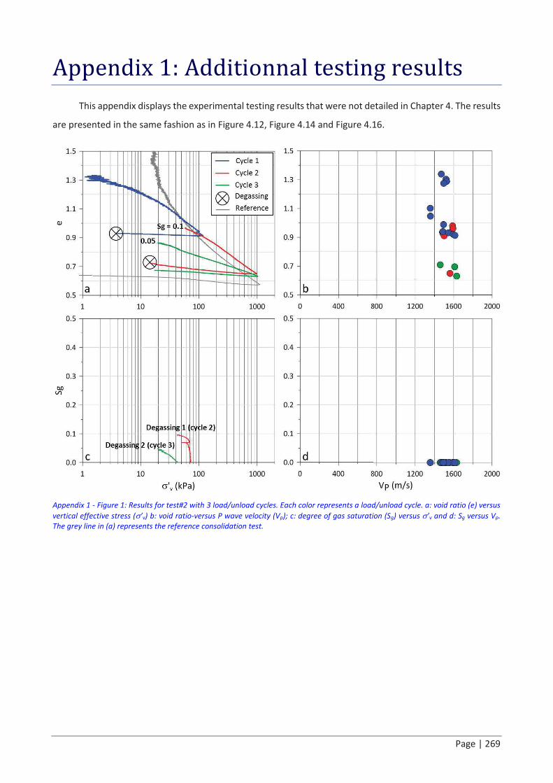
Page | 269
Appendix 1: Additionnal testing results
This appendix displays the experimental testing results that were not detailed in Chapter 4. The results
are presented in the same fashion as in Figure 4.12, Figure 4.14 and Figure 4.16.
Appendix 1 - Figure 1: Results for test#2 with 3 load/unload cycles. Each color represents a load/unload cycle. a: void ratio (e) versus
vertical effective stress (s�v) b: void ratio-versus P wave velocity (Vp); c: degree of gas saturation (Sg) versus s�v and d: Sg versus Vp.
The grey line in (a) represents the reference consolidation test.

Appendix 1 Additionnal testing results
Page | 270
Appendix 1 - Figure 2: Results for test#3 with 2 load/unload cycles. Each color represents a load/unload cycle. a: void ratio (e) versus
vertical effective stress (s�v) b: void ratio-versus P wave velocity (Vp); c: degree of gas saturation (Sg) versus s�v and d: Sg versus Vp.
The grey line in (a) represents the reference consolidation test.

Appendix 1 Additionnal testing results
Page | 271
Appendix 1 - Figure 3: Results for test#4 with 2 load/unload cycles. Each color represents a load/unload cycle. a: void ratio (e) versus
vertical effective stress (s�v) b: void ratio-versus P wave velocity (Vp); c: degree of gas saturation (Sg) versus s�v and d: Sg versus Vp.
The grey line in (a) represents the reference consolidation test.
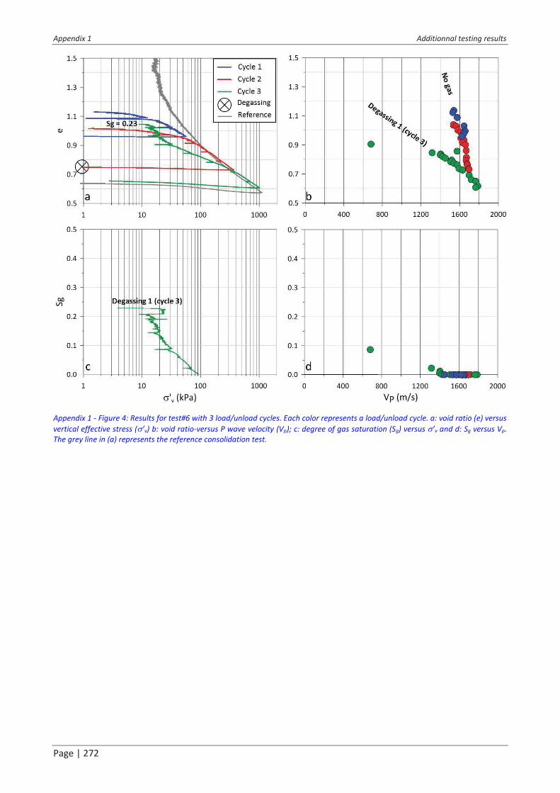
Appendix 1 Additionnal testing results
Page | 272
Appendix 1 - Figure 4: Results for test#6 with 3 load/unload cycles. Each color represents a load/unload cycle. a: void ratio (e) versus
vertical effective stress (s�v) b: void ratio-versus P wave velocity (Vp); c: degree of gas saturation (Sg) versus s�v and d: Sg versus Vp.
The grey line in (a) represents the reference consolidation test.

Appendix 1 Additionnal testing results
Page | 273
Appendix 1 - Figure 5: Results for test#7 with 3 load/unload cycles. Each color represents a load/unload cycle. a: void ratio (e) versus
vertical effective stress (s�v) b: void ratio-versus P wave velocity (Vp); c: degree of gas saturation (Sg) versus s�v and d: Sg versus Vp.
The grey line in (a) represents the reference consolidation test.

Appendix 1 Additionnal testing results
Page | 274
Appendix 1 - Figure 6: Results for test#9 with 3 load/unload cycles. Each color represents a load/unload cycle. a: void ratio (e) versus
vertical effective stress (s�v) b: void ratio-versus P wave velocity (Vp); c: degree of gas saturation (Sg) versus s�v and d: Sg versus Vp.
The grey line in (a) represents the reference consolidation test. The fourth load/unload cycle is not displayed as exsolution was
completed under a constant vertical stress and the results are not relevant in this study. As the sample broke into two separate parts
during the first exsolution, the degree of gas saturation was calculated once the two halves were in contact again (black arrow).

Page | 275
Appendix 2: Published journal articles
This section lists the work presented and/or accepted for publication related to this research.
The first article presents the main results of Chapter 3 and is published in the Journal of Geophysical
Research: Earth Surface and was accepted for publication in February 2019: Blouin, A. et al. (2019) �Evolution
model for the Absheron mud volcano: from in - situ observations to numerical modeling�, Journal of
Geophysical Research: Earth Surface, 124(3), pp. 766�794. doi: 10.1029/2018JF004872. The article is
attached below.
A second article is accepted in the Engineering Geology journal in May 2019 and awaits for editor�s
decision after minor revisions. The article is submitted under the title �Sediment damage caused by gas
exsolution: a key mechanism for mud volcano formation�. It presents the results of Chapter 4.
Results presented in Chapter 5 will be submitted soon as a companion paper of Blouin et al. (2019).
Another article presents results from fieldwork realized over several active mud volcanoes located
onshore Azerbaijan. I participated in the fieldwork in 2017 and in some of the data acquisition and
interpretation and I am therefore co-author of the paper. The purpose of the paper is to understand the
growth of flat-topped MVs combining geophysical data and field observations and structural measurements.
The paper was successfully submitted and accepted in the Marine and Petroleum Geology journal under the
title �Mud volcano growth by radial expansion: examples from onshore Azerbaijan� (Odonne, F. et al. (in
press) �MUD VOLCANO GROWTH BY RADIAL EXPANSION: EXAMPLES FROM ONSHORE AZERBAIJAN�, Marine
and Petroleum Geology.).

Appendix 2 Published journal articles
Page | 276

Evolution Model for the Absheron Mud Volcano: From In
Situ Observations to Numerical Modeling
Arthur Blouin1,2,3 , Patrice Imbert2 , Nabil Sultan1 , and Jean‐Paul Callot3
1Ifremer, Géosciences Marines, LAD, Plouzané, France, 2R&D/EP Total S.A., Pau, France, 3E2S‐UPPA, Laboratoire des
Fluides Complexes et de leurs Réservoirs, IPRA, Université Pau and Pays Adour, Pau CEDEX, France
Abstract The morphology of mud volcanoes (MVs) has been extensively studied over the last few
decades. Although recent research has begun to focus on deep processes and structures, little is known
about mud generation mechanisms. This study aims to investigate the feeder system and formation of an
active kilometer‐scale MV by relying on a 3‐D seismic survey and an in situ data set on the Absheron
anticline (South Caspian Basin). Seismic data show a depleted area in the Anhydritic Surakhany
Formation (ASF), whose mineralogical composition fits with surface mud. Well data show that the ASF
is a succession of evaporitic beds and low‐temperature shales near its fracture pressure. Biostratigraphic
analysis confirms a Pliocene origin for the mud, suggesting that the ASF may be the source.
Numerical modeling of sedimentation coupled with laboratory test results and well sonic logs fairly
reproduces the observed in situ overpressure trend. Two‐dimensional methane diffusion coupled with
overpressure caused by rapid sedimentation highlights the superposition of critical fracturing conditions
with methane‐saturated sediments at the base of the studied MV. The present study demonstrates the
predominant role of fluid overpressure due to sedimentation and gas saturation in the formation of the
Absheron MV, and this is shown to occur as follows: (1) methane migration through the thrust‐related
faults reaching the ASF, accompanied by (2) lateral overpressure, caused by rapid sedimentation,
diffusing along the ASF leading to (3) hydro‐fracturing of overpressured and methane‐saturated
sediments resulting in an important decrease in overpressure, causing (4) gas exsolution and expansion
triggering sediment remobilization.
Plain Language Summary Mud volcanoes have proved to be a real risk for people living near
them (e.g., Lusi catastrophe, Indonesia) and for infrastructures. While their surface morphology is well
understood and their plumbing system is correctly imaged by high‐resolution seismic technology, their
formation mechanisms and their trigger is yet to be understood. The South Caspian Basin is known for the
presence of a large number of active structures. On the Absheron anticline, a giant active mud volcano is
surrounded and covered by a large data set from seismic imaging to sediment cores. From the analysis of the
seismic data, and from diverse measurements on sediments, we were able to locate the source of the mud,
which is shallower than the source for many mud volcanoes in the region. We developed a numerical model
able to reproduce the pore pressure trends recorded at the wells, and it shows that the interaction between
methane‐saturated areas and potential rupture zones is able to explain the mud volcano location. Finally,
based on the different results and observations, a formation model is proposed where hydrofracturing is the
initial trigger for the subsequent gas exsolution and expansion that disaggregate and remobilize weak
sedimentary layers.
1. Introduction
Although mud volcano (MV) surface morphologies have been described in detail and worldwide, both
onshore and offshore, little is known about their evolution and formation processes (e.g., Deville, 2009;
Kopf, 2002; Mazzini & Etiope, 2017). On the other hand, earlier extensive work on fluid emissions at the
surface has improved understanding of subsurface processes and the multiple sourcing of the different
elements forming the material ejected by MVs (Deville, 2009; Kopf, 2002; Mazzini & Etiope, 2017).
Nevertheless, recent technical improvement of geophysical tools, such as high‐resolution 3‐D seismic
imaging, allows for detailed analysis of the MV's rooting system and has opened the way for studying
mud generation processes (Dupuis, 2017; Kirkham et al., 2017a; Stewart & Davies, 2006). Understanding
these generation mechanisms is a key issue for geohazard assessment (e.g., the Lusi catastrophe near©2019. American Geophysical Union.
All Rights Reserved.
RESEARCH ARTICLE10.1029/2018JF004872
Key Points:
• The Absheron mud volcano, unlike
many mud volcanoes in the South
Caspian Basin, is not sourced from
the deep Maykop Formation but
from the Upper Productive Series
• The developed numerical model
shows that an interaction between
methane‐saturated areas and
potential rupture zones allows
locating the mud volcano formation
• A formation model is proposed
where hydrofracturing is the initial
trigger for the subsequent gas
exsolution and expansion that
disaggregate and remobilize weak
sedimentary layers
Correspondence to:
A. Blouin,
Citation:
Blouin, A., Imbert, P., Sultan, N., &
Callot, J.‐P. (2019). Evolution model for
the Absheron mud volcano: From in
situ observations to numerical
modeling. Journal of Geophysical
Research: Earth Surface, 124, 766–794.
https://doi.org/10.1029/2018JF004872
Received 10 SEP 2018
Accepted 18 JAN 2019
Accepted article online 15 FEB 2019
Published online 19 MAR 2019
BLOUIN ET AL. 766

Sidoarjo, Indonesia, since 2006; Tingay et al., 2015), for environmental impacts on seabed ecosystems
(Foucher et al., 2009; Zitter, 2004), targeting drilling areas, and anchoring zones for offshore infrastructures
(Contet & Unterseh, 2015; M. Tingay et al., 2008). Furthermore, one characteristic shared by all MV's around
the world is the presence of gas in the ejected material (Etiope et al., 2009; Hedberg, 1974). Yet it is not clear
at present if the gas is a driver of mud extrusion or a passive actor, captured in the mud during its ascent. If
gas has a driving role in mud extrusion, the understanding of mud generation mechanisms could provide
elements to quantify the volume of expelled methane and therefore evaluate the natural contribution of
MVs to the atmospheric carbon budget (Kopf, 2002).
The South Caspian Basin (SCB), along with its onshore continuation, the Lower Kura Basin, is a prolific
hydrocarbon basin and is also known to hold the highest density of MVs (I. Guliyev et al., 2010; A.
Mazzini & Etiope, 2017). The Absheron gas field is a challenging exploration and production area due to
the presence of a giant active MV. A high‐resolution 3‐D seismic block was acquired in 1996, two exploration
wells were drilled in 1999 and 2011, and a geotechnical campaign with sediment core sampling and in situ
measurements was operated in 2014 for geohazard assessment.
Altogether, we have a rare opportunity to study a MV with a complete set of surface and subsurface data.
Several issues are assessed in this article regarding the stratigraphic source of the mud, the stratigraphic
and lateral location of the mud generation zone, and the physical mechanisms responsible for the
MV formation.
We provide within this study a detailed geomorphological description of the structure as well as the extru-
sion timing based on seismic imaging and other data. Well data and sediment analysis results were inte-
grated into numerical 1‐D and 2‐D models in order to quantify the lateral pressure transmission and the
gas migration effect. Finally, a conceptual evolution model based on these results is proposed.
2. Regional Setting
The SCB is a remnant of the Paratethys Sea that became isolated from the world ocean during the Late
Miocene, Early Pliocene, at the end of the compressive phase of the Alpine tectonic cycle (Bochud, 2011;
Golonka, 2007; Popov et al., 2004). It is now delimited to the north by the Absheron peninsula and ridge,
to the south by the Alborz massif, to the west by the Greater and Lesser Caucasus separated by the Kura
depression, and to the east by the Kopet Dagh (Figure 1; Allen et al., 2002; Brunet et al., 2003; Popov et al.,
2004; Morley et al., 2011).
Since the Middle Miocene, compression uplifted all these massifs and triggered the high‐amplitude folding
of the South Caspian sedimentary series (Allen et al., 2002; Egan et al., 2009; Javanshir et al., 2015; Popov
et al., 2004). This compression initiated the subduction of the South Caspian basement below the basement
of the North Caspian domain, creating the Absheron ridge in‐between (Figure 1; Allen et al., 2002 ; Stewart
& Davies, 2006). The subduction allowed the deposition of more than 8 km of sediments over the last 5.5Myr
based on a representative stratigraphic column of the northwestern part of the basin, which is faster than
sedimentation rates recorded in typical foreland basins (Allen et al., 2002; Morley et al., 2011; Stewart &
Davies, 2006).
The Maykop Formation was deposited from the Late Oligocene to the Early Miocene in a shallow marine
anoxic environment (Golonka, 2007; Hudson et al., 2008; Popov et al., 2004). It is the main hydrocarbon
source rock for the Caspian and Black Sea areas (Allen et al., 2002; Hudson et al., 2008) and acts as the main
décollement level for the high‐amplitude folds of the SCB (Allen et al., 2002; Stewart & Davies, 2006). The
Maykop sediments are mainly organic‐rich clays with a minor fraction of coarser detrital material
(Hudson et al., 2008).
Post‐Maykop Miocene sediments were deposited in a context of global regression until basin isolation
occurred in the Late Miocene. These sediments are shallow marine and lacustrine thick clayey deposits
(Allen et al., 2002; Javanshir et al., 2015).
The Pliocene was dominated by deltaic and lacustrine environments during a regression phase, fed from the
ancestral Kura, Volga, and Amu‐Darya rivers that drained sediments from all the topographic highs sur-
rounding the basin (Abdullayev & Leroy, 2016; Allen et al., 2002). The subduction‐related subsidence at
10.1029/2018JF004872Journal of Geophysical Research: Earth Surface
BLOUIN ET AL. 767

the end of the Miocene accommodated the deposition of thick deltaic deposits containing the regional
hydrocarbon reservoirs and forming the Productive Series (PS; Allen et al., 2002; Javanshir et al., 2015).
The sedimentation rate was very high, reaching 2.4 km/Myr, allowing the deposition of up to 6 km of PS
sediments (Allen et al., 2002; Brunet et al., 2003; Stewart & Davies, 2006). At the top of the Surakhany
Formation (Upper PS), the regression was maximal and evaporitic beds are found in the northern part of
the basin (Javanshir et al., 2015). This interval will hereafter be called Anhydritic Surakhany.
Above the PS, the Akchagyl Suite consists of open marine mudstones. This transgressive interval records the
temporary reconnection of the SCB to the world ocean from 2.4 to 1.6 Ma (Allen et al., 2002; Dupuis, 2017;
Javanshir et al., 2015). From 1.6 Ma to present, deepwater lacustrine and brackish conditions have domi-
nated, forming the Absheron Suite and younger units.
Figure 1. (a) Structural map of the South Caspian region showing themain folds and faults, structural domains, and depo-
centers (modified from Oppo et al., 2014). (b) Regional interpreted deep seismic section, showing the main subsurface
structural elements with the folds above the Maykop detachment level associated in the northern part to deeply rooted
thrusts. The location of the line is shown on the left map by a black line. The red box shows the approximate location of the
Absheron structure (modified from Stewart & Davies, 2006).
10.1029/2018JF004872Journal of Geophysical Research: Earth Surface
BLOUIN ET AL. 768

Information on the stratigraphy of the SCB is synthesized in Figure 2.
The presence of the high total organic carbon Maykop Formation and of the well‐connected PS reservoirs
make the SCB a prolific hydrocarbon basin (Alizadeh et al., 2017; Hudson et al., 2008; Javanshir et al.,
2015). The Maykop Formation generates gas in the deeper part of the basin and is still generating oil
onshore and in the northern margin of the basin (Javanshir et al., 2015). Large‐scale anticlines
(50–150 km long), detached over the overpressured and under compacted Maykop formation (Morley et al.,
2011), form excellent oil and gas traps as hydrocarbons migrate from the deep basin into the onshore
Figure 2. Stratigraphic column for the South Caspian Basin showing the ages, lithology, andmain tectonic and paleo‐geo-
graphical context from Cretaceous to present (modified from Javanshir et al., 2015).
10.1029/2018JF004872Journal of Geophysical Research: Earth Surface
BLOUIN ET AL. 769

heights along the regionally continuous reservoirs (Javanshir et al., 2015). The large‐scale anticline main
growth stage occurred at the end of Pliocene. However, fold‐growth is ongoing although slower (Mosar
et al., 2010).
One hundred and eighty active MVs are listed onshore, and at least the same amount is estimated in the off-
shore part of the SCB (I. S. Guliyev et al., 2001; Kopf, 2002; A. Mazzini & Etiope, 2017; Milkov, 2000). These
structures are mainly located along the crests of anticlines where oil and gas have accumulated in reservoirs
(E. Deville, 2009; Javanshir et al., 2015; A. Mazzini & Etiope, 2017). They are generally considered to be
sourced by the Maykop Formation (Kopf, 2002; Roberts et al., 2010; Stewart & Davies, 2006).
Additionally, Fowler et al. (2000) noticed on the offshore Shah Deniz anticline a close relationship between
the development of folds andMV activity asMVs activated during or after fold initiation and the authors cor-
relate structural growth with MV activity phases.
The Absheron anticline is a NW‐SE oriented, 40‐km‐long fold, located at the northwestern edge of the SCB,
100 km to the south‐west of Baku and 50 km south of the ACG gas field (Figure 1a). Methane was recently
discovered in the Absheron field, and a giant active MV pierces the crest of the structure at the southwestern
limit creating potential hazards for drilling operations (Contet & Unterseh, 2015). Previous studies on the
Absheron anticline evidenced the presence of four mass transport deposits in the Post‐Absheron interval
(Imbert et al., 2014). The most recent mass transport deposit covers the whole anticline with the exception
of the MV location where it stumbles on the northern flank of the volcano. Morphology of the MV in the
upper 500m of the sediment pile is described in Dupuis (2017). The poorly imaged central part is surrounded
by three stacked wedges affected by multiple thrusts. Recent activity of the MV is confirmed by four mud-
flows imaged in the first 100 m below seafloor (BSF).
3. Materials and Methods
3.1. Seismic Data
This study focuses on the Absheron anticline, where an active MV is imaged by a 3‐D seismic survey (limits
and location on Figure 1). The seismic survey covers 650 km2, in water depths ranging from 180 to 700 m.
The seismic sections presented here are from Kirchhoff prestack depth migration reprocessing (Robein,
2010), which was applied on 550 km2 of the seismic survey. The velocity model used in the reprocessing
aimed to improve the imaging of the deep structures (thrust and dips), taking into account the lateral velo-
city variations across the thrust as well as the velocity heterogeneity in the shallow intervals due to the pre-
sence of the MV and free gas (F. Adler, 12/12/2018, personal communication). The model parameterization
is a vertical transverse isotropy that considers the vertical anisotropy imposed by the sedimentary strata
(Robein, 2010). The model was entirely built by tomography inversion (Robein, 2010), and in the deep part,
it was corrected using an interpretative method in order to preserve the structural coherency and to fit the
well data (F. Adler, 12/12/2018, personal communication). The seismic volume is composed by 2,203 inlines
and 2,120 crosslines with 12.5‐m spacing inline and 18.5 crossline. The vertical resolution varies with depth
as it depends on interval velocity. From visual observations of the sections, we estimate a resolution approxi-
mately 20 m in the strata above 2,000 m, progressively decreasing to 150 m at 11 km.
Seismic interpretation was carried out using the Total in‐house software Sismage (Guillon & Keskes, 2004).
From the 3‐D seismic cube, we calculated the seismic coherency attribute, which can be projected on hori-
zontal slices or seismic horizons. Seismic coherency allows to laterally differentiate continuous areas (undis-
turbed deposits) from low continuity zones (faults or MV deposits for instance; Bahorich & Farmer, 1995).
Eachmedium has its own acoustic impedance. Therefore, when a seismic signal reaches a limit between two
media with different impedances, part of the acoustic signal will be reflected (Nely, 1986). A seismic signal
can be decomposed in wavelets, which are characterized by their polarity, their amplitude (peak area), its
period, and its phase (Nely, 1986). Normal polarity is given by the seafloor polarity, which in the data pre-
sented hereafter are a wavelet with a strong central positive amplitude surrounded by two weak negative
amplitudes. Thus, the normal polarity is a strong positive peak enclosed between two weak negative peaks
indicating a stepwise increase in impedance. The opposite shows a stepwise decrease in impedance (Nely,
1986; Ricker, 1953).
10.1029/2018JF004872Journal of Geophysical Research: Earth Surface
BLOUIN ET AL. 770

The presence of free gas is a well‐documented cause of attenuation or data wipe‐out (Benjamin & Huuse,
2017; Graue, 2000). MVs are known to be accompanied by large emissions of gas (Kopf, 2002; A. Mazzini
& Etiope, 2017). Therefore, seismic masking is expected to occur below large structures such as the
Absheron MV (AMV; Benjamin & Huuse, 2017; Graue, 2000). Imaging issues that cannot be settled by
migration algorithms may arise from steep dips (Day‐Stirrat et al., 2010).
Horizons were propagated and named according to stratigraphic limits encountered in the two exploration
wells drilled on the Absheron anticline (Figure 3 for location). These stratigraphic limits are interpreted
based on cuttings analysis and gamma ray, sonic, and resistivity logs.
In parallel of the seismic imaging, high‐resolution bathymetric maps (Figure 3) were acquired using a
multibeam echosounder.
Figure 3. Seismic amplitude map of the seafloor around the Absheron mud volcano. In orange, a high‐amplitude mud-
flow is imaged to the west of the volcano. The dark patch corresponds to the shield composing the mud volcano itself.
On the same map, the location of the different coring and drilling sites are shown. Limits and location of the 3‐D seismic
survey are presented on the regional map of the South Caspian Basin (SCB; Figure 1a). The red lines indicate the location
of the seismic lines presented in Figures 4 to 6. The dotted black polygone is the limit of the zoom shown below, presenting
a detailed image of the seafloor on and around the mud volcano acquired with a multibeam echo sounder. Orange stands
for the shallower areas; green is for the deeper parts.
10.1029/2018JF004872Journal of Geophysical Research: Earth Surface
BLOUIN ET AL. 771

3.2. Sediment Cores and Geotechnical Analysis
3.2.1. Sample Collection
Amarine geological and geotechnical survey of the seabed above the Absheron gas discovery was carried out
in 2014 in order to better constrain and delineate geological hazards associated with the MV (Total proprie-
tary report, G. Dan & S. Po, 12/09/2017, personal communication). The geotechnical/geological survey used
rotary drilling, AUV (autonomous underwater vehicle) sampling with box corer and piston corer, and in situ
geotechnical testing (Cone Penetration Testing [CPT]). Well logging and CPT were performed on two bore-
holes: CH2 was located outside the MV area to provide a stratigraphic reference in continuous series, and
MVF1 sampled on a MV flow (for location see Figure 3).
To improve the characterization of MV deposits, we selected eight samples from different sediment cores.
Table 1 lists the coordinates and depth below seabed of these samples, and Figure 3 shows their location with
respect to the MV. The samples were selected to provide information on the spatial and temporal variability
of the MV deposit (Total proprietary report, G. Dan & S. Po, 12/09/2017, personal communication). Five
samples were selected at three different depths from the same rotary drilling cores MVF1, thus potentially
sampling different mud eruption episodes. One sample fromA13‐PC12a core was taken from the samemud-
flow as the one drilled by MVF1 but at a different location. A different mudflow was sampled on the A13‐
PC11a core at the northern edge of the MV. Finally, a sample was taken from the A13‐BC05 core directly
on the top of the mud shield (see Table 1 for further details and Figure 3 for location).
3.2.2. Mineralogical and Biostratigraphic Analysis of Mud
TheMVF1E RAW sample was separated into two different grain size classes, with a limit at 5 μm, in order to
compare the composition of the clay‐size fraction and the coarser fraction. The >5 μm of the raw sample was
extracted by suspension of fine fractions in water followed by centrifugation.
Eight samples were analyzed using a reference quantitative mineralogy method called MinEval QM (Table
1; Fialips et al., 2018). This method is based on the integration of results from various measurements per-
formed on crushed samples, including X‐ray diffraction on bulk powders and extracted fine fractions, loss
on ignition, X‐ray fluorescence, insoluble residue upon HCl 15% treatment, bulk solid density, and cationic
exchange capacity (see Fialips et al., 2018 for more details). This method performs an initial semiquantitative
mineralogy analysis by Rietveld refinement of the X‐ray diffraction patterns (Rietveld, 1969), and quantifi-
cation is completed applying a dedicated software that uses an iterative approach. The <5‐μm fraction of
MVF1E‐RAW only obtained a semiquantitative mineralogical analysis of clay minerals. The quantity of fine
material obtained after separation was insufficient to perform the complete quantitative study.
Furthermore, a biostratigraphic study by Chevron in 2000 was carried out with the aim of dating the oldest
material composing the mudflows. A series of samples were recovered in and around the volcano location
(green triangles in Figure 3). The samples around the structure were used as age control points. The elements
picked and counted on the different samples are diatoms, pollens, foraminifera, nannofossils, and ostracods.
Initial grain size distribution for the natural mud was determined using the Mastersizer 3000 device for laser
diffraction granulometry (Ryzak & Bieganowski, 2011).
3.2.3. Geotechnical Analysis of Mud
Oedometer tests with permeability measurements were carried out on four samples taken from the GT1‐
MVF1 core (MECA 6‐10‐15‐22 in Table 1 and tests from 1 to 8 in Table 2). Tests were duplicated in order
to check for potential trial mistakes. The samples were selected based on CPT (Das, 2013) data showing at
least four mechanically distinct intervals (Total proprietary report, G. Dan & S. Po, 12/09/2017, personal
communication). The aim of these oedometer tests was to define compressibility characteristics (void ratio
versus effective stress) and to determine the relationship between hydraulic conductivity and void ratio of
the considered sediment intervals (ASTM International, 1996).
The void ratio e changes are tied to the vertical effective stress σ′v by the following compressibility relation:
e ¼ e0−λ lnσ′vσ′v0
! "
(1)
where e0 is the initial void ratio for a reference vertical effective stress σ′v0 and λ is the compression index
depending on the sediments. e0 and λ for the tested samples are shown in Table 2.
10.1029/2018JF004872Journal of Geophysical Research: Earth Surface
BLOUIN ET AL. 772

The permeability relation to void ratio is assumed to be
ln Kð Þ ¼ aeþ b (2)
with K the Darcy permeability (Das, 2013) or hydraulic conductivity (m/s), a and b are constants character-
istic of the tested sediments.
The samples were all reconstituted with an artificial initial water content of around 1.5 wL (wL being the
liquid limit). The wL (Table 2) was determined using the fall cone method (Feng, 2005). Oedometer tests
were conducted using incremental loading according to the ASTM D‐2435 method (ASTM International,
1996). The determination of hydraulic conductivities and permeability coefficients was also possible using
the falling head method (Das, 2013). Using an exponential regression on the obtained measurements is
necessary to obtain a law of the form of equation (2).
In order to artificially characterize the impact of coarse material on mechanical properties, additional oed-
ometer tests were carried out on combined MECA‐16 and MECA‐17 samples (Tables 1 and 2) mixed with a
knownmass of fine sand (80–125 μm); the goal was to obtain their compressibility and permeability in order
to integrate these results in the numerical diffusionmodel. The fractions of coarsematerial added to the sam-
ples were selected based on the net to gross (ratio between sand layer cumulated thickness over total interval
thickness) values calculated from well data.
Table 2
Details on Sample Preparation for Oedometer Rests and Results
Test number Sample σ′vmax (kPa) wL e0 λ Sample preparation
1 MECA‐6 1765.12 0.42 1.95 0.35 1.5 wL water input
2 MECA‐22 1765.12 0.43 1.7 0.34 1.5 wL water input
3 MECA‐10 1765.12 0.56 2.11 0.42 1.5 wL water input
4 MECA‐15 1765.12 0.44 1.79 0.32 1.5 wL water input
5 MECA‐6 1765.12 0.42 2.23 0.36 1.5 wL water input
6 MECA‐22 1765.12 0.43 1.9 0.33 1.5 wL water input
7 MECA‐10 1765.12 0.56 2.58 0.46 1.5 wL water input
8 MECA‐15 1765.12 0.44 2.18 0.34 1.5 wL water input
9 MECA‐16 + 17 + 5% sand 1765.12 0.44 1.38 0.25 1.5 wL water input, mixed samples
10 MECA‐16 + 17 + 10% sand 1765.12 0.44 1.23 0.23 1.5 wL water input, mixed samples
11 MECA‐16 + 17 + 25% sand 1765.12 0.44 1.14 0.20 1.5 wL water input, mixed samples
Table 1
DRX and Mechanical Sample Names and Details Used in This Study
Core name Sample name Type of sample Type of analysis Water depth (m)
Depth below seafloor (m)
Top Bottom
MVF1C DRX1 Core Sample Mineralogy 521 3.53 3.55
MECA‐6 Core Sample Granulometry, oedometer 3.71 3.80
MECA‐10 Core Sample Granulometry, oedometer 5.14 5.22
MVF1D MECA‐15 Core Sample Granulometry, oedometer 522 10.00 10.08
MECA‐16 Core Sample Oedometer 10.41 10.48
MECA‐17 Core Sample Oedometer 10.68 10.75
DRX2 Core Sample Mineralogy 19.00 19.06
MVF1E DRX3 Core Sample Mineralogy 522 33.04 33.06
MECA‐22 Core Sample Granulometry, oedometer 33.08 33.15
RAW>5 μm fraction >5 μm Mineralogy 34.00 34.61
RAW<5 μm fraction <5 μm Mineralogy 34.00 34.61
A13‐PC11A DRX4 Core Sample Mineralogy 467 0.91 1.00
A13‐PC12A DRX5 Core Sample Mineralogy 505 0.11 0.17
A13‐BC05 DRX6 Core Sample Mineralogy 453 0.32 0.36
Note. Total proprietary report, G. Dan and S. Po (12/09/2017, personal communication).
10.1029/2018JF004872Journal of Geophysical Research: Earth Surface
BLOUIN ET AL. 773

3.3. In Situ Well Data and Hydraulic Conductivity Calculations
Stratigraphic information was obtained from the two exploration wells drilled on the Absheron anticline
(Figure 3). Well A reached 6,506‐m TVD/MSL (true vertical depth below mean sea level), while Well B
reached 6,823 TVD/MSL.
Lithology is obtained from cuttings analysis. Pore pressures in shales were estimated from sonic data using
Eaton's (1975) method. Sonic logs were acquired either with wireline or logging while drilling tools depend-
ing on the interval. The StethoScope pressure‐while‐drilling tool (Schlumberger) was used to measure in situ
reservoir pore pressure. Fracturing pressure log is evaluated from leak‐off tests or formation integrity tests
(Lin et al., 2008), as well as downhole mud losses. Wireline tools measured temperatures at different points
either in open hole or cased hole.
The sonic measurements are given as slowness of the acoustic waves, for example, the inverse of acoustic
velocity. Wyllie et al. (1958) gave a relationship between measured velocity of a porous media and its por-
osity ϕ:
1
Vm
¼ϕ
V f
þ1−ϕð Þ
V s
(3)
with Vm indicating the measured acoustic velocity, Vf indicating the acoustic velocity in pore fluid, and Vs
indicating the acoustic velocity in the rock matrix.
As void ratio and porosity are linked through the relation:
e ¼ϕ
1−ϕ(4)
it is possible to calculate hydraulic conductivities K for reservoir layers using the Kozeny‐Carman relation-
ship (Ren et al., 2016):
K ¼ CF1
S2s
γf
μρ2s
e3
1þ eð Þ(5)
where CF is a shape constant around 0.2, Ss is the specific surface area of particles (m2/g) taken here as equal
to 0.5 m2/g, γf is the unit weight of pore fluid (N/m3), ρs (kg/m3) is particle density, and μ is fluid viscosity
(N s/m2).
Therefore, it is possible to estimate the hydraulic conductivity of reservoirs directly from acoustic log data.
Oedometer test results on natural mud allowed calculation of permeability in the shales. From the litholo-
gical log, the column was split into reservoirs and shale intervals. Using equations (2), (3), and (5), we cal-
culate for each defined interval the hydraulic conductivity K. The net to gross ratio (cumulated sand
thickness divided by total interval thickness) was calculated for each drilled formation. The arithmetic aver-
age of hydraulic conductivities gives the horizontal hydraulic conductivity for the considered formation,
while the harmonic average gives its vertical hydraulic conductivity (Das, 2013).
3.4. Numerical Modeling: Sedimentation, Transient Pore Pressure, and Gas Diffusion
3.4.1. 1‐D Sedimentation and Pore Pressure Accumulation
Geological formations remain at hydrostatic pressure after deposition and burial as long as pore fluids are
able to escape up through the overburden or laterally toward the seabed or surface. High permeabilities or
low sedimentation rates help pore water escaping during consolidation. In contrast, when permeability is
low or sedimentation rate is high enough, fluids cannot escape fast enough to keep hydrostatic conditions.
As loading increases through sedimentation, pore water starts to support part of the overburden pressure,
which prevents pores from closing. Thus, normal consolidation is delayed, sediments become undercom-
pacted, and pore pressure increases above hydrostatic conditions. This excess pore pressure is called over-
pressure and this mechanism of overpressure buildup is called compaction disequilibrium (Osborne &
Swarbrick, 1997; Sultan et al., 2004; Swarbrick et al., 2002).
In this work, we calculate in one dimension the overpressure generated (Δu) only by sedimentation effect in
the southern part of the considered section where the sedimentary column is the thickest. The high
10.1029/2018JF004872Journal of Geophysical Research: Earth Surface
BLOUIN ET AL. 774

sedimentation rates observed in the basin are within the strongest recorded worldwide (Allen et al., 2002;
Brunet et al., 2003; Stewart & Davies, 2006). Moreover, high sedimentation rates are considered to be one
of the main overpressure generation mechanism (Osborne & Swarbrick, 1997; Swarbrick et al., 2002).
Therefore, the modeling work focuses on this sedimentation effect as a first approach. The SeCoV3 proprie-
tary software of IFREMER (Sultan et al., 2004) allows quantification of the evolution of pore pressure using a
back analysis based on sedimentation rates, compressibility properties (equation (1)) and permeability evo-
lution with void ratio (equation (2)). In addition to the equations solved by SeCoV3, in the present work we
use a mesh‐update method considering the compressibility of sediments and the mobile position of the
upper boundary (seawater‐sediment interface) at each calculation step.
Sedimentation rates and the model geometry used in this study were calculated using present thicknesses
and ages from Green et al. (2009). These sedimentation rates have been corrected (decompression) for
compaction using Terzaghi compaction equations (Terzaghi, 1943). At the end of sedimentation and
compaction modeling, we applied a trial and error method until the model matched present‐day
observed thicknesses.
Compressibility and permeability properties characterizing each of the defined layers were determined
based on oedometer and permeability tests (Table 2) carried out on natural mudmixed with known fractions
of very fine sand (ASTM International, 1996). The fractions of added sand were selected thanks to net to
gross values calculated from well data (Table 3). The purpose was to model the behavior of layers having dif-
ferent amounts of coarser material.
3.4.2. Two‐Dimensional Transient‐Diffusion Process: Darcy's and Fick's Laws
The two‐dimensional transient dissipation of excess pore pressure generated by the sedimentation
process is considered along a 63‐km‐long and 10‐km‐thick block of the section presented in Figure 11
of Green et al. (2009). We defined the geometrical model with 300 horizontal and 50 vertical nodes by
considering six stratigraphic layers, the fault network around the Absheron fold, and normal faults at
the extrados of the fold.
The excess pore pressure generated by sedimentation and calculated using SeCoV3 was considered as a
boundary condition for the 2‐DDarcy transient flow calculation. The two‐dimensional dissipation and trans-
mission of overpressure is calculated using the 2‐D diffusion equation given by
∂∆u
∂t¼
∂ Dhx∂∆uð Þ
∂x2þ∂ Dhy∂∆u# $
∂y2
! "
(6)
with Δu being the overpressure and Dhx and Dhy, respectively, the horizontal and vertical hydraulic diffusiv-
ities that are calculated directly from the horizontal and vertical hydraulic conductivitiesKx andKy (Table 3).
In addition to the transmission/diffusion of pore pressure, we considered in the present work the molecular
diffusion of dissolved methane. Methane diffusion is calculated using a two‐dimensional diffusion equation
referred to as Fick's law (equation (7)), which allows for the description of diffusion of dissolved molecules
into a solvent (Crank, 1975):
∂C
∂t¼ DC
∂ DC∂Cð Þ
∂x2þ∂ DC∂Cð Þ
∂x2
! "
(7)
with C being the dissolved methane concentration and DC being the methane molecular diffusivity of the
porous water. The effect of tortuosity of pores on molecular diffusivity is considered through the porosity
of the sediment as described by Boudreau (1996).
To solve numerically the 2‐D diffusion equations (equations (6) and (7)), a centered explicit finite difference
discretization scheme is used by considering the initial and boundary conditions for pore pressure and
methane concentration.
Faults are characterized by their own methane molecular diffusivities creating preferential pathways for
methane. Moreover, as the modeled stratigraphic column is formed by a succession of metric‐scale sand
layers and plurimetric shale intervals, a ratio between horizontal and vertical hydraulic conductivities was
integrated based on the results of the hydraulic conductivity calculations at wells (Table 3). This ratio allows
modeling of the natural anisotropy of the sedimentary column due to sand‐shale successions.
10.1029/2018JF004872Journal of Geophysical Research: Earth Surface
BLOUIN ET AL. 775

3.4.3. Hydrofracturing
In some cases, excess pore pressure can exceed the effective least principal stress plus the tensile strength of
the medium allowing hydrofracturing to occur (Alfaro & Wong, 2001). When sediments are only submitted
to the load of the overlying sedimentary cover, the greatest effective stress is vertical (σ′v), whereas the least
effective stress is horizontal (σ′h; Sibson, 2003). Fractures then open in the direction of the least principal
stress and propagate in the direction of the plane perpendicular to the least principal stress (Hubbert &
Willis, 1957). Therefore, in the case of sole loading effects, hydrofractures will propagate vertically.
The vertical effective stress and excess pore pressure are an output of 2‐D Darcy's diffusion equation. The
ratio between fracturing pressure and overburden pressure (lithostatic stress) observed in the well ranges
between 0.83 and 0.99, with an average of 0.9. Consequently, we consider in the present work that hydrofrac-
turing will occur whenever the ratio between excess pore pressure and vertical effective stress (Δu/σ′v)
exceeds 0.9.
4. Results
4.1. Geomorphological Investigation of the AMV
Figures 4 and 5 present two parallel SSW‐NNE sections. Figure 4 runs across the axis of the Absheron fold in
the vicinity of the two exploration wells drilled on the anticline and Figure 5 cuts through the center of the
AMV as located on Figure 3. The ages of five of the seismic horizons that are presented in this study were
calibrated from the stratigraphic results of the well (total proprietary data). We were able to map the top
of Absheron Suite, the top of the Akchagyl Suite, the top of the PS, the top of the Anhydritic Surakhany
Formation (ASF), the Top Diatom Suite, and the top of the Maykop Suite (see Figure 2 for the stratigraphic
column). Seven other seismic horizons were interpreted in order to highlight particular structures such as
normal faults or the morphology of the fold.
The deep part of the Absheron fold is cut by a deep E‐W trending thrust that dies out in the Diatom Suite.
This thrust has more than 2 km of throw, and the northern block overrides the southern block. The thicken-
ing of the interval between Top Diatom and Top Maykop is interpreted as the result of a backthrust system
that would have been inverted later during its history. Another thrust 5 km to the NNW has a throw of only
1 km (Figure 4). The main thrust is responsible for the formation of the Absheron fold, and several folding
phases can be distinguished. The PS interval has a rather uniform thickness of 5 km across the anticline with
only 10% of total thinning from the flanks to the crest of the anticline, indicating a rapid deposition during a
phase of low‐activity for the fold (Figure 4). The Akchagyl Suite presents a thickening toward the southern
flank of the fold of 300 m, corresponding to 60% of its maximum thickness (Figure 4), thus indicating that
growth of the anticline was accelerated during deposition of this interval. Fold activity was still strong during
deposition of the Absheron Suite as the thinning at the crest reaches 650 m for this interval, 35% of its max-
imum thickness. More precisely, the interval between horizons A3 and A2 recorded a thinning of 330m (45%
of maximum thickness), and between A1 and A2, 190 m (40% of maximum thickness; Figure 4). More
Table 3
Results of Hydraulic Conductivity Calculations Based on Sonic‐Log Data and Oedometer Tests on Natural Mud
Layer name
Layer number
in model NTG (%)
Mean void
ratio from logs Kh (m/s) Kv (m/s) Kh/Kv
Void ratio ranges
from 1‐D model
K ranges from
oedometer
tests (m/s) Model kx/ky
Novocaspian‐
Absheron
Layer 5 5 0.33 5.03E−07 2.27E−10 2212 2.73–0.36 5.01E−07 to 3.53E−10 2200
Surakhany Layer 4 8 0.18 3.18E−09 2.13E−10 15 0.43–0.24 7.50E−10 to 4.17E−10 15
Sabunchy Layer 3 12 0.14 1.27E−09 1.95E−10 6 0.22–0.21 4.70E−10 to 4.56E−10 6
Balakhany‐Fasila Layer 2 24 0.17 5.16E−10 2.57E−10 2 0.27–0.24 7.78E−10 to 7.05E−10 2
NKG Layer 1 8 0.17 2.18E−10 2.10E−10 1 0.24–0.22 4.17E−10 to 3.92E−10 1
Note. NTG is the net to gross, being the ratio between total sand thickness over total interval thickness. Themean void ratio is calculated from the sonic log (equa-tion (3)) and Kh (horizontal hydraulic conductivity) and Kv (vertical hydraulic conductivity) result respectively from arithmetic and harmonic average of calcu-lated hydraulic conductivities on individual sand or shale layers using equation (5). The 1‐D‐sedimentation model gives a range of void ratio for eachstratigraphic interval, corresponding to hydraulic conductivity ranges on oedometer test results obtained for different sand fraction content (Table 2).Measured and calculated K's are in the same ranges of magnitude.
10.1029/2018JF004872Journal of Geophysical Research: Earth Surface
BLOUIN ET AL. 776

recently, during Post‐Absheron times, the fold reactivated and another 450 m of thinning (45% of maximum
thickness) is visible from Top Absheron horizon to the seafloor (Figure 4). Therefore, sediment thinning at
the crest of the anticline indicates that fold activity really started at the Akchagyl times, when it reached its
climax. During the Absheron Suite deposition, the fold activity was intense for a longer time interval, and
recent intense fold activity was also recorded in the Post Absheron interval.
Besides, normal faults on the extrados of the fold form a complex network from the thrust up to the Upper PS
(Figure 4). The backthrust was then inverted to form the main observed normal fault.
The AMV is located in the SE part of the 3‐D seismic survey. Figure 3 shows the seismic amplitude of the
seafloor horizon, with a color‐scale set to outline high and low amplitude zones. Orange stands for the high-
est amplitude and darker areas correspond to lower amplitude zones. The high‐resolution bathymetric map
(Figure 3) reveals present seafloormorphology related to recentMV activity. Near‐surfacemorphology of the
MV was already detailed by Dupuis (2017), with the presence of three main wedges (Transparent Facies and
Chaotic Facies on Figure 5) and at least four recent mudflows evidenced on seismic data.
ThisMV is a subcircularmud shield, 4 to 5 km in diameter (Figure 3). It is surrounded by a gently dipping apron
(average outward slope from 4 to 6°); the relief above the surrounding seafloor does not exceed 70m (Figure 3).
The highest area is a relatively flat plateau, but at a closer look reveals at least four gently mounded circular
structures, 0.5‐ to 1‐km diameter (Figure 3); we interpret these as the loci of most recent mud emission. At
thewestern edge of themud shield, a 12‐km‐long, 1.5‐ to 3‐km‐wide high‐amplitude patch extends from the vol-
cano to the west before following the natural slope toward the south of the Absheron seismic survey (Figure 3).
This high‐amplitude patchwas already described as a giantmudflow byDupuis (2017). This mudflow shows up
strongly on seabed amplitude maps, indicating that is closer to seabed than the resolution of the data set.
Interpretation of the section running through the center of the AMV (Figure 3 for location) is given in
Figure 5. The first obvious observation is the presence of a large seismically transparent body spreading hor-
izontally in the first 500 m BSF. Four wedges of this feature are imaged at the SSW from the center of the
Figure 4. Uninterpreted and interpreted seismic line crossing the anticline near the two exploration wells A and B; it was used as reference for horizon picking for
this study. A deep thrust cores the Absheron anticline, and another thrust, smaller, is also visible at the NNE of the section. From the thickness differences between
the flanks and the crest of the structure, we note that folding started during the Akchagyl deposition. The main growing phases are during deposition of the
Absheron Suite (A3‐A1) and later during the Post‐Absheron times. See Figure 3 for location.
10.1029/2018JF004872Journal of Geophysical Research: Earth Surface
BLOUIN ET AL. 777

volcano. These interdigitations reunite at the center of the structure and form one large seismically
transparent zone from the seafloor down to 1 km BSF. The shallowest digitation follows exactly the
seafloor seismic horizon and is less than 50 m thick. As it was sampled notably with the box core A13‐
BC05 (Figure 3), this transparent area can directly be interpreted as mudflow deposits forming the MV
edifice (green patch on Figure 5). Below 2 km at the center of the structure, a seismically transparent
cone goes down to 7 km. This area could reveal the masking effect of the low velocity mass formed by the
shallower mud deposits that may also be saturated with gas, preventing the acoustic signal from
propagating below. Another seismic facies can be discriminated from the blind signal: the blue patch can
be described as a chaotic signal. This area is located between the mudflows and host sediments.
Moreover, the deeply rooted thrusts described on Figure 4, are still imaged, yet not as clearly because of the
seismic masking. Nevertheless, the AMV is centered above the exact vertical of the main thrust (Figure 5).
The first mudflows imaged were deposited during the post‐Absheron interval, between seismic horizons
H3 and the Seafloor. No activity is recorded before H3. Consequently, the AMV seems to have been initiated
after the end of the Absheron folding phase, during the post‐Absheron folding phase.
Normal faults are imaged near the blind cone (Figure 5). They cross the Absheron Suite and end in the
Upper PS, near the Anhydritic Surakhany interval.
After the time of extrusion, we addressed the issue of the primary source of the mud by identifying a possible
depletion zone (Kirkham et al., 2017b; Stewart & Davies, 2006). In order to alleviate the seismic masking, we
looked at lines crossing the volcano away from its center. Figure 6 presents aWNW‐ESE seismic section, per-
pendicular to the section shown in Figure 5 and crossing the volcano 2 km away from its center. The section
crosses the distal part of both transparent facies bodies and of the chaotic facies body from 0.5 to 2 km. The
mudflow deposits appear 200 m above the H3 seismic horizon. The Top Absheron horizon is truncated by
the chaotic mass. Deeper seismic horizons, from Absheron to Top PS, bend downwards, forming a bowl
shape particularly visible on tracked horizons A1 and A3. The Anhydritic Surakhany horizon and the
200‐m‐thick interval below are truncated by downlapping younger intervals. Another truncated interval,
400 m thick, is imaged between 3,400 and 3,800 m and contained approximately the lower interval of the
Upper PS, below the ASF. From 3,800 m to deeper, horizons become continuous and flat again.
Figure 5. Uninterpreted and interpreted seismic line across the active mud volcano. The first 2 km are clearly imaged and show four seismically transparent wedges,
corresponding to mudflows. A chaotic signal below can be discriminated from the blind signal and is interpreted as reworked sediments. The rooting system is blind,
maybe due to a masking effect from the low velocity mud deposits. Near the blind area, some normal faults are present between 1.5 and 3 km. A deep thrust is
coring the main anticline. The activation of the mud volcano is contemporaneous to the main folding phase (see text and Figure 4 for details and Figure 3 for location).
10.1029/2018JF004872Journal of Geophysical Research: Earth Surface
BLOUIN ET AL. 778
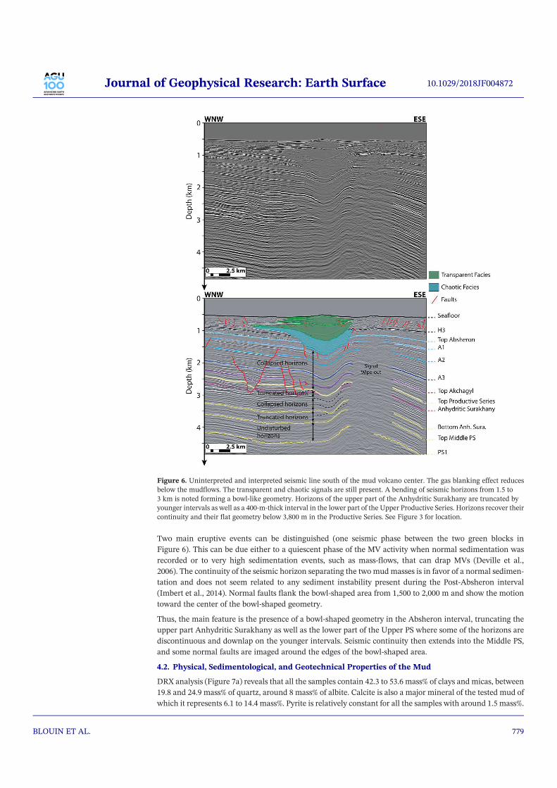
Two main eruptive events can be distinguished (one seismic phase between the two green blocks in
Figure 6). This can be due either to a quiescent phase of the MV activity when normal sedimentation was
recorded or to very high sedimentation events, such as mass‐flows, that can drap MVs (Deville et al.,
2006). The continuity of the seismic horizon separating the two mudmasses is in favor of a normal sedimen-
tation and does not seem related to any sediment instability present during the Post‐Absheron interval
(Imbert et al., 2014). Normal faults flank the bowl‐shaped area from 1,500 to 2,000 m and show the motion
toward the center of the bowl‐shaped geometry.
Thus, the main feature is the presence of a bowl‐shaped geometry in the Absheron interval, truncating the
upper part Anhydritic Surakhany as well as the lower part of the Upper PS where some of the horizons are
discontinuous and downlap on the younger intervals. Seismic continuity then extends into the Middle PS,
and some normal faults are imaged around the edges of the bowl‐shaped area.
4.2. Physical, Sedimentological, and Geotechnical Properties of the Mud
DRX analysis (Figure 7a) reveals that all the samples contain 42.3 to 53.6 mass% of clays and micas, between
19.8 and 24.9 mass% of quartz, around 8 mass% of albite. Calcite is also a major mineral of the tested mud of
which it represents 6.1 to 14.4 mass%. Pyrite is relatively constant for all the samples with around 1.5 mass%.
Figure 6. Uninterpreted and interpreted seismic line south of the mud volcano center. The gas blanking effect reduces
below the mudflows. The transparent and chaotic signals are still present. A bending of seismic horizons from 1.5 to
3 km is noted forming a bowl‐like geometry. Horizons of the upper part of the Anhydritic Surakhany are truncated by
younger intervals as well as a 400‐m‐thick interval in the lower part of the Upper Productive Series. Horizons recover their
continuity and their flat geometry below 3,800 m in the Productive Series. See Figure 3 for location.
10.1029/2018JF004872Journal of Geophysical Research: Earth Surface
BLOUIN ET AL. 779

The clay fraction was analyzed in detail (Figure 7b) and is composed of 38 to 49% interstratified
illite/smectite, 29 to 38% Illite and/or micas, and around 15% kaolinite. The rest is composed of around
5% chlorite and less than 2% smectite.
More details are provided by the results of the two fractions of the same samples (Raw > 5 μm; Raw < 5 μm;
see Table 1). Even when separating the clay‐size particles from the rest, the coarser fraction is still composed
of 31.8 mass% of clay minerals (Figure 7) showing the presence of clay aggregates or claystone clasts larger
than 5 μm that were not separated during suspension and centrifugation processes (Figure 7). Themaximum
amount of calcite and the only significant gypsum content are reached on this fraction with respectively 23.6
and 5.4 mass%. Comparatively with the <5‐μm fraction, it also contains a greater part of chlorite with 23% of
the clay fraction. Further analysis on the chlorite fraction would be necessary to conclude on its origin and
the reasons for this variability as acid treatment destroys chlorite minerals.
In the fraction of particles less than 5 μm in diameter (Figure 7b), there is only 20% illite and/or micas but
also more kaolinite and chlorite (23% and 13% respectively). Illite is known to form at a higher temperature
than interstratified illite/smectite (Pollastro, 1993), which means that the finer fraction is composed of a
smaller portion of high‐temperature clay minerals than the unseparated samples but is also composed of
more kaolinite and chlorite.
Peaks of carbonates have been observed in the coarser fraction of MVF1E as well as the BC05‐DRX5 and the
PC12a‐DRX4. Sample BC05 was recovered from the top of the mud shield, while PC12a comes from the top
of themudflow (Figure 3 and Table 1). This peak could be the result of the formation of authigenic carbonate
crusts due to methane bubbling through fresh mud after an eruptive phase or at the top of the structure dur-
ing a dormant phase (Kopf, 2002; Zitter, 2004).
Thus, the Absheron mud is essentially composed of clay minerals and quartz particles (Figure 7). Clay
minerals are not only contained in the matrix as fractions of particles larger than 5 μm also contain more
than 30% of clays.
Biostratigraphic results on pollens and ostracods show a clear difference between samples collected on the
MV or on mudflows and background samples (Figure 3 for location). Samples from the MV shield and the
mudflow contain pollens from Miocene to Recent and ostracods from Late Miocene (PS). Conversely, back-
ground sediments when not barren contain pollens from the Pleistocene and Holocene ostracods (Post‐
Absheron). Diatoms were only found in shallow background sediments and mudflows, with Pleistocene
to Holocene taxa. The presence of diatoms identical to those of the background in mudflows and their
absence from shield samples may indicate that the flows remobilized surface sediments on their way down-
slope and mixed with them. Nannofossil results are not considered reliable due to the poorness of elements
present in the samples. Put together, these biostratigraphic results seem to indicate that the mud expelled at
the AMV only comes from the PS.
Samples for oedometer tests were initially selected based on MVF1 CPT data from the Absheron mudflow
(Figure 3 for location, Total proprietary report, G. Dan & S. Po, 12/09/2017, personal communication).
CPT curves (cone resistance, pore pressure, and friction) present four intervals with distinct evolution of
the three measured parameters. We suppose that these distinct tendencies are related to different intrinsic
mechanical behavior of the mud intervals and oedometer tests were run on one selected reconstituted sam-
ple per interval at water content of around 1.5 wL in order to test this hypothesis (Tables 1 and 2). Details on
preparation and results of these oedometer tests are presented in Table 2. Oedometer tests presented in
Figure 8a show no distinct behavior except for the MECA 10 sample, which also has a slightly different gran-
ulometric curve than the other three selected samples (Figure 8c). Indeed, theMECA 10 sample has a greater
fraction of fine material (from 2 to 10 μm) and less coarse fraction (from 30 to 300 μm) than the three other
samples. This also matches with the high initial void ratio and the high compressibility of theMECA 10 sam-
ple with respect to the other samples (Figure 8a). Likewise, natural sediments show similar hydraulic con-
ductivity with void ratio results except for MECA‐10 that has a slightly lower permeability trend in
accordance with the lower granulometry of this sample (Figures 8b and 8c).
MECA 6‐15‐22 compressibility curve (equation (8)) was considered as representative of all the other natural
mud samples given the very low variability between the three different samples (Figure 8a) taken from dif-
ferent depths of the MVF1 core (Table 1).
10.1029/2018JF004872Journal of Geophysical Research: Earth Surface
BLOUIN ET AL. 780

e ¼ 1:64−0:16 lnσ’v
σ’v0
! "
(8)
Permeability results showed no real differences between the different natural samples except for MECA‐10
(Figure 8b), and a global linear regression for the other natural samples between ln(K) and the void ratio was
adopted:
ln Kð Þ ¼ 3:06e−22:48 (9)
Figure 8a shows that oedometer tests carried out on natural mud with a coarser fraction are characterized by
a relatively low compressibility with a low initial void ratio (Table 2). At around 1,000 kPa of vertical effec-
tive stress, the different compressibility curves converge at the same void ratio (Figure 8a). The permeability
globally increases with the fraction of coarser material with the same parallel trend as natural
sediments (Figure 8b).
Figure 7. (a) Whole rock mineralogical analysis for all the samples collected except the less than 5‐μm fraction of the
MVF1E‐RAW sample. The main elements composing the mud are clearly clay minerals and quartz particles. (b)
Mineralogical composition of clay for all the samples collected except the MVF1E‐RAW>5 μm. Globally, clay fraction is
mainly composed by up to 50% of interstratified illite/smectite, 30% of Illite and/or micas, 15% of kaolinite, and a
minor part of chlorite and smectite. The less than 5‐μm fraction of the MVF1E‐RAW sample differs from the whole
samples as they have less illite and/ormicas, andmore kaolinite and chlorite. See Figure 3 for locationmap and Table 1 for
details of samples.
10.1029/2018JF004872Journal of Geophysical Research: Earth Surface
BLOUIN ET AL. 781

4.3. In Situ Lithology, Temperature, and Excess Pore Pressure Derived From In Situ Well Data
The Post‐Absheron interval and the Upper part of the Absheron Suite are composed of claystone.
Interstratified claystones and siltstones form the rest of the Absheron Suite and the Akchagyl Suite. The
ASF extends from 2,501 to 2,887 m TVD/MSL in well B and 2,522 to 2,905 m TVD/MSL in well A. It is com-
posed of claystone and evaporitic beds (mainly anhydrite and halite) and a minor part of siltstone. Over the
400m of drilled Anhydritic Surakhany, 30% of evaporitic beds were encountered with individual thicknesses
ranging from less than 1 to 8 m. Finally, the rest of the PS varies from claystone with rare pluri‐decimetric to
metric beds of siltstone to sandstone in the Surakhany (Upper PS) to interstratified claystones, siltstones, and
sandstones in the Lower PS. Some of the sandstone beds reach 15 m in thickness.
Figure 8. (a) Oedometer tests with void ratio (e) versus vertical effective stress (σ′v) for the different tested samples. For
the natural samples, only the MECA‐10 has a higher compressibility and a higher initial void ratio than the other sam-
ples. The input of coarser materials reduce the initial void ratio and reduce the compressibility of the samples.
(b) Hydraulic conductivity (k) versus void ratio (e) resulting from oedometer test and falling head method results for the
different samples analyzed. Again, MECA‐10 has a lower permeability than other natural samples, which fit the same
trend. The input of coarser material increases the hydraulic conductivity but the general trend stays parallel to natural
samples. (c) Cumulative granulometry for the natural samples showing that MECA 10 is finer than the three other sam-
ples. See Figure 3 and Table 1 for more details on the samples.
10.1029/2018JF004872Journal of Geophysical Research: Earth Surface
BLOUIN ET AL. 782
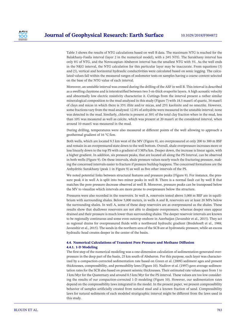
Table 3 shows the results of NTG calculations based on well B data. The maximum NTG is reached for the
Balakhany‐Fasila interval (layer 2 in the numerical model), with a 24% NTG. The Surakhany interval has
only 8% of NTG, and the Novocaspian‐Absheron interval has the smallest NTG with 5%. As the well ends
in the NKG interval, the NTG calculation for this particular layer may be inaccurate. From equations (3)
and (5), vertical and horizontal hydraulic conductivities were calculated based on sonic logging. The calcu-
lated values fall within the measured ranges of oedometer tests on samples having a coarse content selected
on the base of the NTG value of each interval.
Moreover, an unstable interval was crossed during the drilling of the ASF in well B. This interval is described
as a swelling claystone and is interstratified between two 5‐m‐thick evaporite layers. A high acoustic velocity
and abnormally low electric resistivity characterize it. Cuttings from the interval present a rather similar
mineralogical composition to the mud analyzed in this study (Figure 7) with 18.5 mass% of quartz, 34 mass%
of clays and micas in which there is 35% illite and/or micas, and 25% kaolinite and no smectite. However,
some fractions vary from themud analyzed: 12.8% of anhydrite weremeasured in the unstable interval; none
was detected in the mud. Similarly, chlorite is present at 30% of the total clay fraction when in the mud, less
than 10% was measured as well as calcite, which was present at 20 mass% at the considered interval, when
around 10 mass% was measured in the mud.
During drilling, temperatures were also measured at different points of the well allowing to approach a
geothermal gradient of 16 °C/km.
Both wells, which are located 9.5 km west of the MV (Figure 9), are overpressured at only 200 to 300 m BSF
and remain in an overpressured state down to the well bottom. Overall, shale overpressure increases more or
less linearly down to the top PS with a gradient of 3 MPa/km. Deeper down, the increase is linear again, with
a higher gradient. In addition, six pressure peaks, that are located all along the PS Interval, can be observed
in both wells (Figure 9). On these intervals, shale pressure values nearly reach the fracturing pressure, mak-
ing the concerned intervals easier to fracture if pressure buildup happens. The concerned formations are the
Anhydritic Surakhany (peak 1 in Figure 9) as well as five other intervals of the PS.
We noted potential links between structural features and pressure peaks (Figure 9). For instance, the pres-
sure peak 4 in well A is split into two minor peaks in well B. There is a normal fault cut by well B that
matches the pore pressure decrease observed at well B. Moreover, pressure peaks can be transposed below
the MV to visualize which intervals are more prone to overpressure below the structure.
Pressures were also recorded in the reservoirs. In well A, reservoirs tested above 5,000 m BSF are in equili-
brium with surrounding shales. Below 5,000 meters, in wells A and B, reservoirs are at least 20 MPa below
the surrounding shales. In well A, some of these deep reservoirs are as overpressured as the shales. These
results show that shallower reservoirs are not able to dissipate overpressure, whereas deeper ones appear
drained and their pressure is much lower than surrounding shales. The deeper reservoir intervals are known
to be regionally continuous and some even outcrop onshore in Azerbaijan (Javanshir et al., 2015). They act
as regional drains for overpressured fluids with a northward hydraulic gradient (Bredehoeft et al., 1988;
Javanshir et al., 2015). The sands in the northern area of the SCB are at hydrostatic pressure, while an excess
hydraulic head creates deeper in the center of the basin.
4.4. Numerical Calculations of Transient Pore Pressure and Methane Diffusion
4.4.1. 1‐D Modeling
The first step of the numerical modeling was a one‐dimension calculation of sedimentation‐generated over-
pressure in the deep part of the basin, 25 km south of Absheron. For this purpose, each layer was character-
ized by a compaction‐corrected sedimentation rate based on Green et al. (2009) sediment ages and present
thicknesses, compressibility, and permeability laws (Figure 10). Nadirov et al. (1997) gave average sedimen-
tation rates for the SCB also based on present seismic thicknesses. Their estimated rate values span from 1 to
3 km/Myr for the Quaternary and around 0.5 km/Myr for the PS interval. These values are too low consider-
ing the results of our compaction‐corrected 1‐D modeling (Figure 10). However, our sedimentation rates
depend on the compressibility laws integrated in the model. In the present paper, we present compressibility
behavior of samples artificially created from natural mud and a known fraction of sand. Compressibility
laws for natural sediments of each modeled stratigraphic interval might be different from the laws used in
this study.
10.1029/2018JF004872Journal of Geophysical Research: Earth Surface
BLOUIN ET AL. 783

The calculation runs over 5 Myr, during which 9,600 m of compacted sediments have been deposited. As
compression laws for mixed mud and very fine sands were measured for the first 1,800 kPa of vertical effec-
tive stress, at higher effective stress, the void ratio may reach negative values in some layers. In order to avoid
this type of problem, we set a minimum limit for the void ratio at 0.1 in the software to obtain a compressi-
bility trend similar to the ones presented by Chong and Santamarina (2016). Permeability laws for natural
mud and mudmixed with very fine sands obtained from oedometer test results were integrated to character-
ize each stratigraphic interval (Figures 8a and 8b). The validity of the permeability laws was confirmed by
the calculations on sonic logging (Table 3).
Figure 10 shows the porosity profile versus depth at the end of the sedimentation history. It gives a good
representation of how sediments have compacted during the sedimentation history. The overpressure plot
shown in Figure 10 corresponds to the overpressure generated by high sedimentation rates in the deepest
part of the basin. Overpressure rises rapidly with depth in the low permeability layer 5 as overpressure can-
not be evacuated and transmitted rapidly to the whole interval. The increase is slower from layer 4 down
because of higher permeability. Finally, overpressure increases with a very low gradient from layer 2 below,
layer 2 having the highest permeability.
4.4.2. 2‐D Modeling
The second part of the modeling consisted of creating a structural model for two‐dimensional diffusion of
overpressure and methane. The structural model presented in Figure 11 is based on the work of Green
et al. (2009) and on the fault network observed on the reference section in Figure 4. The initial section
presented by Green et al. (2009) was only reproduced from the deeper part of the basin to the Absheron
Ridge, where the seafloor is shallowest. The direction is the same as the section presented in Figure 1b.
The total length of the section is 55 km, and its maximum depth 9.6 km. Faults shown in Figure 11 are
Figure 9. 3‐D view of the two parallel seismic lines distant of 9.5 km. The right one is described in Figure 5. The left one in
Figure 4. The pressure peaks numbered from 1 to 6 and observed on the pressure logs recorded on the two exploration
wells are reported in front of the corresponding interval on seismic.
10.1029/2018JF004872Journal of Geophysical Research: Earth Surface
BLOUIN ET AL. 784

meant to represent not only the fault surfaces (localized thin shear zone) but also to the damage zone
surrounding them. We estimated the thickness of the damage zone based on the work of Savage and
Brodsky (2011), who relate the damaged thickness around a fault to the throw of the fault. With a
total throw about 2 kilometers for the main thrust, a damage zone of a few hundred meters is
expected. In the present work, a damage zone of 300 m is considered as representative of the fault zones.
Figure 11 shows the boundary conditions used for the numerical calculation of methane and pore pressure
diffusions. No lateral or vertical exchange of pore pressure and methane with the outside of the model is per-
mitted through the laterally impermeable southern and northern borders and the vertically impermeable
upper and lower borders. The seawater has a fixed pore pressure of 0 kPa and a methane concentration of
10−5 mM (millimolar, 1 molar corresponding to a solution of 1 mol/L of concentration), which is a mean
oceanic value (Lamontagne et al., 1973). The pore pressure calculated in one dimension from sedimentation
with SeCoV3 (Figure 10) is imposed at the southern border of the model, where the sedimentary column is
the thickest. Finally, a methane concentration of 10−3 mM is fixed at the bottom of the fault network,
methane being generated in the Maykop Formation, the regional source rock, the deepest layer represented
in the model.
Pressure and methane migration calculation were run over 5 Myr. Results of the diffusion equation resolu-
tion (equations (6) and (7)), in terms of overpressure migration, are shown in Figure 12a. Methane concen-
tration and ratio between overpressure and vertical effective stress are shown together in Figure 12b in order
to compare possible hydrofractured zones with high dissolved methane saturated areas.
Overpressure (Δu) propagated from south to north of the model at different diffusion rates. Indeed,
depending mainly on permeability laws, overpressure will propagate more or less quickly and in different
directions. For instance, in layer 5 overpressure did not accumulate (Figure 12a). This layer being the
youngest, it maintained a high void ratio and so a higher permeability. The effect is amplified by the
ratio between horizontal and vertical permeabilities. Layer 5 having a ratio of 2,200 (Table 3), the
horizontal permeability in the model is 2,200 times larger than the permeability defined by oedometer
test results. Therefore, in layer 5, pressure diffusion is mainly horizontal and the seawater condition
(no overpressure) has significant impact on the overpressure values of this interval. From layer 4
Figure 10. Results of the one‐dimensional sedimentation modeling. On the left, porosity versus depth trend at the end of the 5 Myr of sedimentation with corrected
sedimentation rates for each layer. On the right, overpressure versus depth trend at the end of the 5 Myr of sedimentation.
10.1029/2018JF004872Journal of Geophysical Research: Earth Surface
BLOUIN ET AL. 785

below, the pressure is mainly diffused laterally creating a pressure front. At a given distance from the
south of the model, where overpressure was injected from one‐dimension sedimentation modeling
(Figure 11), overpressure is larger in layer 4 than in other layers reproducing the pressure peaks
observed at the wells (Figure 9).
Faults and associated damage zones were designed to rapidly diffuse methane therefore artificially reprodu-
cing methane advection through fractured zones. Methane was injected at the base of the fault network with
a concentration of 10−3mM (Figure 11). Methane molecular diffusivity in the rest of the model is 3 orders of
magnitude lower than in faults. As a result, methane rapidly saturated the area adjoining the faults, and then
diffused slowly through the sedimentary column until saturating an area nearly 2 km wide around the fault
network (Figure 12b). The ratio of overpressure over vertical effective stress (Δu /σ′v) is higher in layer 5, par-
ticularly in the north of the model. As it is the shallowest interval, σ′v is the lowest of the model. Besides,
little overpressure accumulation was possible in layer 5. Nevertheless, values are high at the top of the layer
4, where the ratio varies between 0.5 and 0.6. So we expect critical values in the area of high methane satura-
tion at the Absheron crest.
5. Discussion
5.1. What Is the Stratigraphic Source of the Mud?
The geomorphological description of the AMV evidenced a bowl‐shaped geometry below the mass extruded
through the Absheron interval (Figure 6). This feature is formed by the Anhydritic Surakhany horizons that ter-
minate as truncations (Catuneanu et al., 2009) below the younger seismic horizons of the Upper PS. Truncations
are also observed 500 m below, in the lower part of the Upper PS. Horizon continuity resumes in the Middle PS.
This particular geometry was already described and corresponds to a depleted area forming a potential former
mud generation zone (Dupuis, 2017; Kirkham et al., 2017b; Stewart & Davies, 2006). The presence of two trun-
cated intervals (Figure 6) indicates that there may have been several mud generation stages.
The unstable interval drilled in the Anhydritic Surakhany has a mineralogical composition similar to the
mud analyzed in this study (Figure 7), with nearly 50% of clay minerals. Mud sampled at the seafloor is
poorer in anhydrite, chlorite, and calcite than the unstable interval analyzed in the ASF. The mineralogical
differences may be explained by the different paths and histories of the samples. Mud was driven upward
Figure 11. Structural model based on Green et al. (2009) work and on the fault network observed in Figure 4. The line follows the same trend as the seismic section
of Figure 1b. Eight layers extend along the section corresponding to different sedimentation rates, compaction laws, and permeability trends (see Figure 10). The
layers NKG, Balakhany‐Fasila, Sabunchy, Surakhany, and quaternary are named layers 1 to 5, respectively, in other figures. Numbers showed at the limits of the
model correspond to limit conditions imposed for the diffusion of pore pressure and methane.
10.1029/2018JF004872Journal of Geophysical Research: Earth Surface
BLOUIN ET AL. 786
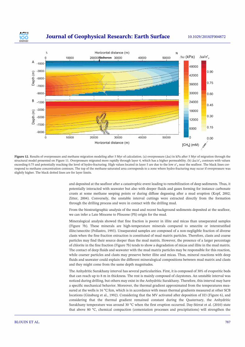
and deposited at the seafloor after a catastrophic event leading to remobilization of deep sediments. Thus, it
potentially interacted with seawater but also with deeper fluids and gases forming for instance carbonate
crusts at some methane seeping points or during diffuse degassing after a mud eruption (Kopf, 2002;
Zitter, 2004). Conversely, the unstable interval cuttings were extracted directly from the formation
through the drilling process and were in contact with the drilling mud.
From the biostratigraphic analysis of the mud and recent background sediments deposited at the seafloor,
we can infer a Late Miocene to Pliocene (PS) origin for the mud.
Mineralogical analysis showed that fine fraction is poorer in illite and micas than unseparated samples
(Figure 7b). These minerals are high‐temperature minerals compared to smectite or interstratified
illite/smectite (Pollastro, 1993). Unseparated samples are composed of a non‐negligible fraction of diverse
clasts when the fine fraction extraction is constituted of mud matrix particles. Therefore, clasts and coarse
particles may find their source deeper than the mud matrix. However, the presence of a larger percentage
of chlorite in the fine fraction (Figure 7b) tends to show a degradation of micas and illite in the mud matrix.
The contact of deep fluids and seawater with the mud matrix particles may be responsible for this reaction,
while coarser particles and clasts may preserve better illite and micas. Thus, mineral reactions with deep
fluids and seawater could explain the different mineralogical compositions between mud matrix and clasts
and they might come from the same depth magnitudes.
The Anhydritic Surakhany interval has several particularities. First, it is composed of 30% of evaporitic beds
that can reach up to 8 m in thickness. The rest is mainly composed of claystones. An unstable interval was
noticed during drilling, but others may exist in the Anhydritic Surakhany. Therefore, this interval may have
a specific mechanical behavior. Moreover, the thermal gradient approximated from the temperatures mea-
sured at the wells is 16 °C/km, which is in accordance with mean thermal gradients measured at other SCB
locations (Ginsburg et al., 1992). Considering that the MV activated after deposition of H3 (Figure 6), and
considering that the thermal gradient remained constant during the Quaternary, the Anhydritic
Surakhany temperature was around 30 °C when the first eruption occurred. Day‐Stirrat et al. (2010) state
that above 80 °C, chemical compaction (cementation processes and precipitations) will strengthen the
Figure 12. Results of overpressure and methane migration modeling after 5 Myr of calculation. (a) overpressure (Δu) in kPa after 5 Myr of migration through the
structural model presented on Figure 11. Overpressure migrated more rapidly through layer 4, which has a higher permeability. (b) Δu/σ′v contours with values
exceeding 0.75 and potentially reaching the level of hydro‐fracturing. High values located in layer 5 are due to the low σ′v near the seafloor. The black lines cor-
respond to methane concentration contours. The top of the methane‐saturated area corresponds to a zone where hydro‐fracturing may occur if overpressure was
slightly higher. The black dotted lines are for layer limits.
10.1029/2018JF004872Journal of Geophysical Research: Earth Surface
BLOUIN ET AL. 787

mudstone fabric and this process is irreversible, so the mudstone can no longer behave in a ductile way.
Thus, the ASF would have been well within the temperature range where ductile deformation
is conceivable.
Finally, overpressure logs show that the Anhydritic Surakhany forms a pressure peak at both wells
(Figure 9). Rupture in this interval would happen earlier than in other formations for a given pressure
increase or stress decrease. The fact that highly overpressured mudstones are blocked between meter‐thick
layers of evaporites may explain the weak behavior of some layers. As compaction water cannot be expelled
vertically because of evaporites, these layers are likely to stay undercompacted and overpressured.
From these observations and measurements it seems plausible to conclude that Upper PS, and more pre-
cisely the ASF, is the source of the solid fraction of the mud expelled at the AMV.
5.2. How Do the Field Pore Pressure Measurements Compare to the Model?
It is quite clear on pressure logs that pressure regimes are completely different in shales and in reservoirs.
Indeed, shales are highly overpressured all along the well, following a trend nearly parallel to the litho-
static pressure from the Top Akchagyl to the Bottom PS. In the bottom part of the wells (from the PS2
seismic horizon downward), overpressure level in shales remains rather constant, while reservoir pres-
sures are nearly hydrostatic. Javanshir et al. (2015) describe similar pressure regime and magnitudes in
the neighboring Shah Deniz fold. The Upper PS there have equal sandstone and shale overpressures
and as the reservoir facies become more abundant and continuous in the Bottom PS, they become less
overpressured. Therefore, in Shah Deniz and Absheron, the deep reservoirs seem to act as permeable
drains as they allow overpressure to dissipate. The fact that shale pressure is also affected shows that
dewatering might occur in the thinner shale intervals contained in the Bottom PS. Indeed, the abundance
of permeable reservoirs would allow compaction water to be drained away from the shales, reducing their
pressure. There is lateral pressure transmission from the deep part of the basin to the edges through
regional‐scale reservoirs (Javanshir et al., 2015), from the south to the north of the sections presented in
Figure 9.
However, pressure horns in Absheron shales are not recorded in the data of Javanshir et al. (2015). Some
intervals of the PS of Absheron wells are more overpressured than the rest of the stratigraphic interval.
These peaks bring the corresponding intervals to pressure values between 5 and 10MPa below hydrofractur-
ing pressure in wells located 9.5 km from the MV center. The difference between hydrofracturing pressure
and shale pressure may be even smaller near the MV, or it may have been smaller in the past, before MV
activation. Therefore, they represent weak areas where a local rise in overpressure through clay dehydration
or tectonic overpressuring for instance (Osborne & Swarbrick, 1997), or a drop in effective stress (erosion or
fold growth and crestal uplift) could generate hydrofractures.
Pressures recorded in the two wells are not exactly the same: in the southern well (Well A), shale pressure
decreases more gently within the Bottom PS and reservoir pressures are higher. Moreover, pressure horns
are stronger in well B (to the north). Differential sedimentation between the deep basin located at the
south of the Absheron anticline and the northern edge of the basin where less sediments accumulate
could explain this phenomenon (Grosjean et al., 2009; Javanshir et al., 2015). As pressure transmission
is oriented roughly from the south to the north of the anticline, the northern side of the anticline would
accumulate more overpressure in the shales, whereas reservoirs would be more drained than in the
southern flank. This phenomenon was also noted at the neighboring Shah Deniz anticline (Javanshir
et al., 2015).
Two‐dimensional model sections reproducing the main features of the pressure plots are shown on
Figure 12. The overpressure rises down to 2,000 and 5,000‐mdeep depending on the location. Then overpres-
sure remains constant at 30 MPa at the Absheron location and even decreases to 25 MPa when reaching the
bottom part of the PS where highly continuous and abundant reservoir facies are present. Moreover, the
numerical modeling results emulate the Top Surakhany pressure horn. Yet the modeling results underesti-
mate the overpressure at the Absheron location (Figure 12a) as they are not in accordance with overpressure
values recorded at the wells. Indeed, from Top Surakhany down, overpressure reaches values between 20
and 50 MPa. The discrepancy between measured and calculated overpressures may be related to the com-
pressibility and permeability laws applied to the model, which were obtained from artificial
10.1029/2018JF004872Journal of Geophysical Research: Earth Surface
BLOUIN ET AL. 788

(reconstituted) sandy‐clayey samples and not from natural samples from the different stratigraphic layers.
Besides, the considered source of overpressure is related to fast sedimentation and might not be sufficient
to model the natural pressure conditions of the Absheron anticline. Indeed, additional sources of pore pres-
sure may play an important role and are yet to be considered in the modeling work.
However, and as a first approach, the present calculation was able to reproduce the main overpressure
trends visible at the wells.
5.3. How Does Methane Diffusion Interact With Excess Pore Pressure Accumulation?
Modeling results shows that high values of Δu /σ′v fit with high dissolved methane concentrations and
occur around the fault network below the AMV (Figure 12b). The consequence of high Δu /σ′v causing
hydrofracturing may be an important decrease in pore pressure leading to methane exsolution and expan-
sion (Duan & Mao, 2006) and generation of overpressured mud. Gas exsolution in sediments has proved
to be a critical factor controlling sediment damage. Indeed, experience on gassy sediment core recovery in
deep water shows important damage and loss of structure during the core ascent to the surface and asso-
ciated hydrostatic pore reduction (Sultan et al., 2012). Loss of acoustic signal corresponding to the
presence of free gas correlates with dramatic decrease of the yield stress ratio illustrating the damage
made to the sediments.
Moreover, the presence of normal faults at the anticline crest between the Upper PS and the Top Absheron
(Figure 4) shows that the state of stress where the primary source of mud was identified was extensive at the
time when the AMV formed. If compressive state was dominating at these time and location, the observed
faults must have been thrusts. Therefore, σ1 (the maximum principal stress) was certainly vertical, so the
least principal stress was horizontal. Fractures open in the direction of the least principal stress and then pro-
pagate in a plane perpendicular to this direction (Hubbert &Willis, 1957). Thus, hydrofractures generated at
the time of the MV formation above the mud generation zone are expected to be vertical.
A present‐day studied example of clastic extrusion triggering displays similar results. Indeed, the Lusi disas-
ter, whose 2006 triggering cause is still a matter of debate between an earthquake and drilling issues (A.
Mazzini et al., 2007; M. Tingay et al., 2008, 2017), was initiated by the combination of under‐compaction/
overpressure in the source layer and the presence of dissolved and free gas. According to Davies et al.
(2008), fractures generated by drilling activities have caused an important decrease in pore pressure and
the consequence was gas exsolution and expansion, overpressured mud generation, and the extrusion of
mud to the surface (Davies et al., 2008). However, Mazzini et al. (2012) proposed a hydrothermal source
for the gas, and yet Lusi triggering is already explained by gas flowing in undercompacted and
overpressured sediments.
Thus, we suggest that the theoretical mechanism we propose for mud generation and extrusion with a com-
bination of potential fracture zones and gas‐saturated areas would also be applicable to the Absheron fold,
where the studied MV is located.
5.4. What Is the most Plausible Sequence for the Formation of the AMV?
Based on previous observations and conclusions, a qualitative formation model for the AMV is proposed.
This model is developed in five main phases:
Phase 1: rapid deposition of the PS (over 3.5 km in 2 Myr) above the gas‐mature Maykop Formation that
would generate hydrocarbons migrating slowly through the sedimentary column (Figure 13‐1). Maykop
Formation started generating gas during the Late Miocene in the Shah Deniz region located less than
50 km from Absheron gas discovery (Figure 2.9 in Alizadeh et al., 2017). Moreover, the deposition of the
ASF proves that the sea level must have been lower than nowadays at the end of the PS deposition.
Phase 2: folding started during deposition of the Akchagyl Suite. It is linked to the propagation of a deep
thrust terminating in the Maykop formation and linked to normal faults related to the fold formation.
Methane migration is then focused into the faulted core of the anticline (Figure 13‐2). The folding also
has the effect of generating preferential rupture zones at its crest (Figure 13‐2). Indeed, at the anticline crest,
σ′v is lower than on the flanks. Besides, as more space is available for sediment deposition in the surrounding
synclines and in the deeper part of the basin, overpressure is generated and transmitted toward the
10.1029/2018JF004872Journal of Geophysical Research: Earth Surface
BLOUIN ET AL. 789

Absheron location. Overpressure generation and transmission as well as lower σ′v at the flanks increases the
Δu /σ′v ratio thereby increasing pore gas solubility.
Phase 3: Δu /σ′v ratio reaches the hydro‐fracturing threshold (Figure 13‐3), leading to a significant decrease
in pore pressure.
Phase 4: hydrofracturing triggers gas exsolution and expansion in gas‐saturated and mechanically weak
layers such as ASF (Figure 13‐4). Exsolution remobilizes the weak interval, generating mud.
Overpressured and low‐density mud is then transported to the seafloor provoking the first mud extrusion.
As gas, mixed with sediments and water, migrates up the hydrofracture network, methane expands amplify-
ing the process and potentially eroding fracture walls (Figure 13‐4).
Phase 5: the process goes on with gas exsolution propagating in the Anhydritic Surakhany, depleting this
layer continuously. Collapse of the upper strata into the depleted area creates the rather flat and low topo-
graphy volcano (Figure 13‐5). The extruded mud slowly degasses at the seafloor.
Phase 6: quiescent and active phases of the MV alternates, creating a complex interdigitation geometry
where normal sedimentation predominates during quiescent phases of the volcano. Further depletion hap-
pens in the source, triggering more collapse, while more mud is extruded at the seafloor (Figure 13‐6).
The initial trigger of this MV is not related to gas, as hydrofracturing due to overpressure buildup and weak-
ness of the fold‐crest initiates the succession of events. However, in this conceptual model, methane would
have three essential effects.
Gas needs to saturate the porous network in its dissolved state before hydrofracturing in order to provoke
remobilization of sediments. Exsolution of methane weakens and disaggregates host sediments (Sultan
et al., 2012; M. R. P. Tingay et al., 2015).
As free gas has very low density (typically about 1/1,000 of that of water in normal conditions), it will flow
toward the surface (Brown, 1990), carrying the mud away (solid particles and formation water).
Finally, as gas goes up into the pipe, it expands (Brown, 1990), accelerating the mud ascent, sustaining mud
pressure, and eroding fracture walls, creating clasts, to end‐up with mud breccia extrusion at the surface.
Thus, methane exsolution is the key to mud formation but also the main driver for mud remobilization
toward the surface due to its low density and expansion capacity. Initial rupture is essential in order to start
the chain reaction and methane expansion and exsolution will maintain the pipes open and even
enlarge them.
5.5. Limits and Perspectives of the Study
This conceptual formation model of MVs closely fits with observations and analysis of the available data set
and is partly based on the numerical modeling results presented earlier.
However, Improvements May Be Made at Several Levels:
Data Set: For instance, the seismic masking prevents direct observation of the center of the volcano's
plumbing system. Reprocessing of the data was attempted several times and with different methods and
approaches, but it remains challenging due to the presence of gas‐charged mud and free gas. The available
biostratigraphic analyses are not quantitative and for further precision on the mud origin quantitative ana-
lyses of the fauna and flora in mud will be necessary. Analysis of the clasts will also help to refine the mud
origin.
Numericalmodeling: The compressibility laws used in the current model could be improved to consider
soil compressibility for the highest stress range (Chong & Santamarina, 2016). In the present work and in
order to avoid negative void ratio values, the software limits the minimum void ratio to 0.1. In the present
model, pore pressures generated by sedimentation and pressure transmission are not calculated simulta-
neously. Overpressure due to sedimentation is calculated over 5 Myr of sedimentation history and is inte-
grated as a boundary condition into the 2‐D Darcy's and Fick's diffusion equations. The next step would
be to integrate both sedimentation and diffusion processes into one unique 2‐D model. Finally, the model
does not simulate the post‐hydrofracturing processes causing gas exsolution and overpressured mud expul-
sion. Gas exsolution and expansion processes will have to be integrated into this model in order to reproduce
MV initiation.
10.1029/2018JF004872Journal of Geophysical Research: Earth Surface
BLOUIN ET AL. 790
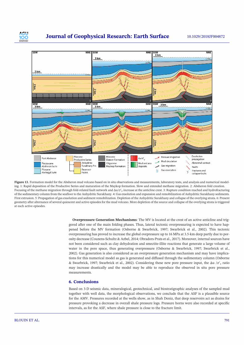
Overpressure Generation Mechanisms: The MV is located at the crest of an active anticline and trig-
gered after one of the main folding phases. Thus, lateral tectonic overpressuring is expected to have hap-
pened before the MV formation (Osborne & Swarbrick, 1997; Swarbrick et al., 2002). This tectonic
overpressuring has proved to increase the global ovepressure up to 16 MPa at 3.5‐km deep partly due to por-
osity decrease (Couzens‐Schultz & Azbel, 2014; Obradors‐Prats et al., 2017). Moreover, internal sources have
not been considered such as clay dehydration and smectite‐illite reactions that generate a large volume of
water in the pore space, thus generating overpressure (Osborne & Swarbrick, 1997; Swarbrick et al.,
2002). Gas generation is also considered as an overpressure generation mechanism and may have implica-
tions for this numerical model as gas is generated and diffused through the sedimentary column (Osborne
& Swarbrick, 1997; Swarbrick et al., 2002). Considering these new pore pressure input, the Δu /σ′v ratio
may increase drastically and the model may be able to reproduce the observed in situ pore pressure
measurements.
6. Conclusions
Based on 3‐D seismic data, mineralogical, geotechnical, and biostratigraphic analyses of the sampled mud
together with well data, the morphological observations, we conclude that the ASF is a plausible source
for the AMV. Pressures recorded at the wells show, as in Shah Deniz, that deep reservoirs act as drains for
pressure provoking a decrease in overall shale pressure logs. Pressure horns were also recorded at specific
intervals, as for the ASF, where shale pressure is close to the fracture limit.
Figure 13. Formation model for the Absheron mud volcano based on in situ observations and measurements, laboratory tests, and analysis and numerical model-
ing. 1: Rapid deposition of the Productive Series and maturation of the Maykop formation. Slow and extended methane migration. 2: Absheron fold creation.
Focusing of the methane migration through fold‐related fault network and Δu/σ′v increase at the anticline crest. 3: Rupture condition reached and hydrofracturing
of the sedimentary column from the seafloor to the Anhydritic Surakhany. 4: Gas exsolution and expansion and remobilization of Anhydritic Surakhany sediments.
First extrusion. 5: Propagation of gas exsolution and sediment remobilization. Depletion of the Anhydritic Surakhany and collapse of the overlying strata. 6: Present
geometry after alternance of several quiescent and active episodes for the mud volcano. More depletion of the source and collapse of the overlying strata is triggered
at each active episodes.
10.1029/2018JF004872Journal of Geophysical Research: Earth Surface
BLOUIN ET AL. 791

Based on these observations, a numerical model with 2‐D‐diffusion equations was applied on a basin scale
section. Sedimentation‐related overpressures underestimate by 50% the pressures measured in the wells
but reproduce fairly well the observed trends. Additional sources of in situ overpressure generation (i.e., clay
dehydration and transformation), which are not included in the current model, may explain the discrepancy
between themodel prediction and the pore pressure values of wells. Themain observationmade through the
numerical model is the superposition of methane‐saturated areas with potential hydrofracturing zones.
Indeed, hydrofracturingmay produce a drastic decrease in pore pressure, allowing gas exsolution and expan-
sion. Based on the present model results, on experimental results of gassy‐sediment behavior in which the
gas exsolution damages the sediment and reduces its mechanical strength and on the Lusi disaster studies,
we conclude that the superposition of potential hydrofracturing areas and gas‐saturated zones can explain
that the AMV activated at the crest of the anticline.
As a result, we propose a conceptual evolutionary model for the AMV as follows: initial stages of folding
focus methanemigration into the anticline crest bringing methane to the upper geological layers andmainly
to the Anhydritic Surakhany Fm. Pore pressure accumulation and its lateral migration through the
Anhydritic Surakhany Fm. promote hydrofracturing at the location of the AMV, causing a decrease in pore
pressure. Those conditions lead to methane exsolution and expansion and to upward remobilization of the
already weak Anhydritic Surakhany interval, generating low density and overpressured mud. During mud
ascent, gas bubbles expand, splintering fracture walls and incorporating clasts into the mud. Finally, extru-
sion at the seafloor happens where the mud slowly expels methane. As extrusion goes on, a collapse of the
overlying strata into the depleted mud generation zone forms.
Therefore, even though the trigger point for the whole MV formation process in our model is hydrofractur-
ing, clay‐rich sediments have to be initially saturated with methane in order to generate mud. The methane
is essential and has three main roles: exsolution allows creating the mud from weak layers, its low density
decreases the mud one and accelerate its upward flow to the surface, and gas expansion sustains mud over-
pressure and causes splintering of gas‐saturated fracture walls creating clasts.
With the available dense data set, we evidence that in order to form the AMV, a combination of three factors
is required: high pore pressure, gas saturation and clay‐rich sediments. Recent work on the Lusi eruption
also demonstrated the importance of the same factors in a different geological environment. Therefore,
detecting the presence of those three factors may help understand the preconditioning conditions of
MV's formation.
ReferencesAbdullayev, E., & Leroy, S. A. G. (2016). Provenance of clay minerals in the sediments from the Pliocene Productive Series, western South
Caspian Basin. Marine and Petroleum Geology, 73, 517–527. https://doi.org/10.1016/j.marpetgeo.2016.03.002
Alfaro, M. C., & Wong, R. C. K. (2001). Laboratory studies on fracturing of low‐permeability soils. Canadian Geotechnical Journal, 38(2),
303–315. https://doi.org/10.1139/cgj‐38‐2‐303
Alizadeh, A. A., Guliyev, I. S., Kadirov, F. A., & Eppelbaum, L. V. (2017). Geosciences of Azerbaijan Volume II: Economic Geology and
Applied Geophysics (Vol. II). Basel, Switzerland: Springer International Publishing. https://doi.org/10.1007/978‐3‐319‐40493‐6
Allen, M. B., Jones, S., Ismail‐Zadeh, A., Simmons, M., & Anderson, L. (2002). Onset of subduction as the cause of rapid Pliocene‐
Quaternary subsidence in the South Caspian basin. Geology, 30(9), 775–778. https://doi.org/10.1130/0091‐7613(2002)030<0775:
OOSATC>2.0.CO;2
ASTM International. (1996). D 2435‐96 ‐ Standard test method for one‐dimensional consolidation properties of soils. American Society for
Testing and Materials, (August), 196–205. doi: https://doi.org/10.1520/D2435‐96
Bahorich, M. S., & Farmer, S. L. (1995). 3‐D seismic discontinuity for faults and stratigraphic features: The coherence cube. In SEG
Technical Program Expanded Abstracts 1995 (pp. 93–96). Houston, TX: Society of Exploration Geophysicists. https://doi.org/10.1190/
1.1887523
Benjamin, U. K., & Huuse, M. (2017). Seafloor and buried mounds on the western slope of the Niger Delta.Marine and Petroleum Geology,
83, 158–173. https://doi.org/10.1016/j.marpetgeo.2017.02.023
Bochud, M. (2011). Tectonics of the Eastern Greater Caucasus in Azerbaijan, (Vol. 30, p. 207). Fribourg, Switzerland: Université de Fribourg.
Boudreau, B. P. (1996). The diffusive tortuosity of fine‐grained unlithified sediments. Geochimica et Cosmochimica Acta, 60(16), 3139–3142.
https://doi.org/10.1016/0016‐7037(96)00158‐5
Bredehoeft, J. D., Djevanshir, R. D., & Belitz, K. R. (1988). Lateralfluid flow in a compacting sand‐shale sequence: South Caspian basin.American
Association of Petroleum Geologists Bulletin, 72(4), 416–424. https://doi.org/10.1306/703C9A1E‐1707‐11D7‐8645000102C1865D
Brown, K. M. (1990). The nature and hydrogeologic significance of mud diapirs and diatremes for accretionary systems. Journal of
Geophysical Research, 95(B6), 8969. https://doi.org/10.1029/JB095iB06p08969
Brunet, M.‐F., Korotaev, M. V., Ershov, A. V., & Nikishin, A. M. (2003). The South Caspian Basin: a review of its evolution from subsidence
modelling. Sedimentary Geology, 156(1‐4), 119–148. https://doi.org/10.1016/S0037‐0738(02)00285‐3
Catuneanu, O., Abreu, V., Bhattacharya, J. P., Blum, M. D., Dalrymple, R. W., Eriksson, P. G., et al. (2009). Towards the standardization of
sequence stratigraphy. Earth‐Science Reviews, 92(1–2), 1–33. https://doi.org/10.1016/j.earscirev.2008.10.003
10.1029/2018JF004872Journal of Geophysical Research: Earth Surface
BLOUIN ET AL. 792
Acknowledgments
Total S.A. is owner of the seismic and
well data used and presented in this
paper. Please contact the Research and
Development team of Total for
information and potential access to this
data (SCR/RD, Total CSTJF, Avenue
Larribau, 64000 Pau). Sediment
analysis results used in this study can be
downloaded by following this link:
https://doi.org/10.6084/m9.
figshare.7448153. To access the SeCoV3
software and the input parameters,
please directly download it here https://
github.com/ArthurBlouin/SeCoV3.git.
This study was realized in the scope of
the PhD of Arthur Blouin under the
joint direction of the Pau University
(UPPA), Ifremer and Total S.A. The
authors would like to thank Claire
Fialips for the mud mineralogy
analysis, Jérémie Gaillot for the help
with biostratigraphy interpretation, and
Mickaël Rovere for the help rendered
during compressibility/permeability
analyses.

Chong, S.‐H., & Santamarina, J. C. (2016). Soil Compressibility Models for a Wide Stress Range. Journal of Geotechnical and
Geoenvironmental Engineering, 142(6), 06016003), 1–7. https://doi.org/10.1061/(ASCE)GT.1943‐5606.0001482
Contet, J., & Unterseh, S. (2015). Multiscale site investigation of a giant mud‐volcano offshore Azerbaijan—Impact on subsea field devel-
opment. Offshore Technology Conference, OTC‐25864(Mv), 1–10. doi: https://doi.org/10.4043/25864‐MS
Couzens‐Schultz, B. A., & Azbel, K. (2014). Predicting pore pressure in active fold‐thrust systems: An empirical model for the deepwater
Sabah foldbelt. Journal of Structural Geology, 69(PB), 465–480. https://doi.org/10.1016/j.jsg.2014.07.013
Crank, J. (1975). The mathematics of diffusion. https://doi.org/10.1016/0306‐4549(77)90072‐X
Das, B. M. (2013). Principles of geotechnical engineering, (7th ed.. Journal of Chemical Information and Modeling (Vol. 53)). Boston,
Massachusetts: CENGAGE Learning. https://doi.org/10.1017/CBO9781107415324.004
Davies, R. J., Brumm, M., Manga, M., Rubiandini, R., Swarbrick, R., & Tingay, M. (2008). The East Java mud volcano (2006 to present): An
earthquake or drilling trigger? Earth and Planetary Science Letters, 272(3–4), 627–638. https://doi.org/10.1016/j.epsl.2008.05.029
Day‐Stirrat, R. J., McDonnell, A., & Wood, L. J. (2010). Diagenetic and seismic concerns associated with interpretation of deeply buried
mobile shales. Shale Tectonics: AAPG Memoir, 93, 5–28. https://doi.org/10.1306/13231306M93730
Deville, E. (2009). Mud volcano systems. In N. Lewis, & A.Moretti (Eds.), Volcanoes: Formation, eruptions andmodelling (pp. 95–125 (404)).
Hauppauge, New York: Nova Science Publishers.
Deville, E., Guerlais, S. H., Callec, Y., Griboulard, R., Huyghe, P., Lallemant, S., et al. (2006). Liquefied vs stratified sediment mobilization
processes: Insight from the South of the Barbados accretionary prism. Tectonophysics, 428(1–4), 33–47. https://doi.org/10.1016/j.
tecto.2006.08.011
Duan, Z., & Mao, S. (2006). A thermodynamic model for calculating methane solubility, density and gas phase composition of methane‐
bearing aqueous fluids from 273 to 523 K and from 1 to 2000 bar. Geochimica et Cosmochimica Acta, 70(13), 3369–3386. https://doi.org/
10.1016/j.gca.2006.03.018
Dupuis, M. (2017). Processus de mise en place et évolution des systèmes de volcans de boue. Université Lille 1 ‐ Sciences et technlogies.
Eaton, B. A. (1975). The equation for geopressure prediction from well logs. In Fall meeting of the Society of Petroleum Engineers of AIME (5
pp.). Dallas, Texas: Society of Petroleum Engineers. https://doi.org/10.2118/5544‐MS
Egan, S. S., Mosar, J., Brunet, M.‐F., & Kangarli, T. (2009). Subsidence and uplift mechanisms within the South Caspian Basin: Insights
from the onshore and offshore Azerbaijan region. Geological Society, London, Special Publications, 312(1), 219–240. https://doi.org/
10.1144/SP312.11
Etiope, G., Feyzullayev, A., & Baciu, C. L. (2009). Terrestrial methane seeps and mud volcanoes: A global perspective of gas origin.Marine
and Petroleum Geology, 26(3), 333–344. https://doi.org/10.1016/j.marpetgeo.2008.03.001
Feng, T. W. (2005). Reappraisal of the fall cone test. In Proceedings of the 16th International Conference on Soil Mechanics and Geotechnical
Engineering, (Vol. 16, pp. 357–360). Osaka, Millpress Science Publishers/IOS Press. https://doi.org/10.3233/978‐1‐61499‐656‐9‐357
Fialips, C. I., Labeyrie, B., Burg, V., Mazière, V., Munerel, Y., Haurie, H., et al. (2018). Quantitative mineralogy of Vaca Muerta and alum
shales from Core chips and drill cuttings by calibrated SEM‐EDS mineralogical mapping. DOI: https://doi.org/10.15530/urtec‐2018‐
2902304
Foucher, J. P., Westbrook, G., Boetius, A., Ceramicola, S., Dupré, S., Mascle, J., et al. (2009). Structure and drivers of cold seep ecosystems.
Oceanography, 22(1), 92–109. https://doi.org/10.5670/oceanog.2009.11
Fowler, S. R., Mildenhall, J., Zalova, S., Riley, G., Elsley, G., Desplanques, A., & Guliyev, F. (2000). Mud volcanoes and structural devel-
opment on Shah Deniz. Journal of Petroleum Science and Engineering, 28(4), 189–206. https://doi.org/10.1016/S0920‐4105(00)00078‐4
Ginsburg, G. D., Guseynov, R. A., Dadashev, A. A., Ivanova, G. A., Kazantsev, S. A., Solov'yev, V. A., et al. (1992). Gas hydrates of the
southern Caspian. International Geology Review, 34(8), 765–782. https://doi.org/10.1080/00206819209465635
Golonka, J. (2007). Geodynamic evolution of the South Caspian Basin. Oil and Gas of the Greater Caspian Area, 55, 17–41. https://doi.org/
10.1306/1205844St551463
Graue, K. (2000). Mud volcanoes in deepwater Nigeria. Marine and Petroleum Geology, 17(8), 959–974. https://doi.org/10.1016/S0264‐
8172(00)00016‐7
Green, T., Abdullayev, N., Hossack, J., Riley, G., & Roberts, A. M. (2009). Sedimentation and subsidence in the South Caspian Basin,
Azerbaijan. Geological Society, London, Special Publications, 312(1), 241–260. https://doi.org/10.1144/SP312.12
Grosjean, Y., Zaugg, P., Gaulier, J.‐M., & Total S.A. (2009). Burial hydrodynamics and subtle hydrocarbon trap evaluation: From the
Mahakam Delta to the South Caspian Sea. International Petroleum Technology Conference Held in Doha, Qatar, 7‐9 December 2009,
1–12.
Guillon, S., & Keskes, N. (2004). Sismage and the 3D visualization at Total. In AAPG International Conference (pp. 1–3).
Guliyev, I., Aliyeva, E., Huseynov, D., Feyzullayev, A., & Mamedov, P. (2010). Hydrocarbon potential of ultra deep deposits in the South
Caspian Basin. In AAPG European Region Annual Conference (Vol. 1, p. 66). Kiev, Ukraine.
Guliyev, I. S., Feizulayev, A. A., & Huseynov, D. A. (2001). Isotope geochemistry of oils from fields & mud volcanoes in the South Caspian
Basin, Azerbaijan. Petroleum Geoscience, 7(2), 201–209. https://doi.org/10.1144/petgeo.7.2.201
Hedberg, H. D. (1974). Relation of methane generation to Undercompacted shales, shale diapirs, and mud volcanoes. AAPG Bulletin, 58(4),
661–673. https://doi.org/10.1306/83D91466‐16C7‐11D7‐8645000102C1865D
Hubbert, M. K., & Willis, D. G. (1957). Mechanics of hydraulic fracturing. Society of Petroleum Engineers, 210, 153–163. Retrieved from
http://archives.datapages.com/data/specpubs/methodo2/data/a075/a075/0001/0200/0239.htm
Hudson, S. M., Johnson, C. L., Efendiyeva, M. A., Rowe, H. D., Feyzullayev, A. A., & Aliyev, C. S. (2008). Stratigraphy and geochemical
characterization of the Oligocene‐Miocene Maikop series: Implications for the paleogeography of Eastern Azerbaijan. Tectonophysics,
451(1–4), 40–55. https://doi.org/10.1016/j.tecto.2007.11.045
Imbert, P., Geiss, B., & Fatjó de Martín, N. (2014). How to evacuate 10 km3 of mud: Saturate with gas and decrease the pressure! Geo‐
Marine Letters, 34(2–3), 199–213. https://doi.org/10.1007/s00367‐014‐0357‐3
Javanshir, R. J., Riley, G. W., Duppenbecker, S. J., & Abdullayev, N. (2015). Validation of lateral fluid flow in an overpressured sand‐shale
sequence during development of Azeri‐Chirag‐Gunashli oil field and Shah Deniz gas field: South Caspian Basin, Azerbaijan.Marine and
Petroleum Geology, 59, 593–610. https://doi.org/10.1016/j.marpetgeo.2014.07.019
Kirkham, C., Cartwright, J., Hermanrud, C., & Jebsen, C. (2017a). The genesis of mud volcano conduits through thick evaporite sequences.
Basin Research, 30(2), 217–236. https://doi.org/10.1111/bre.12250
Kirkham, C., Cartwright, J., Hermanrud, C., & Jebsen, C. (2017b). The spatial, temporal and volumetric analysis of a large mud vol-
cano province within the Eastern Mediterranean. Marine and Petroleum Geology, 81, 1–16. https://doi.org/10.1016/j.
marpetgeo.2016.12.026
Kopf, A. J. (2002). Significance of mud volcanism. Reviews of Geophysics, 40(2), 1005. https://doi.org/10.1029/2000RG000093
10.1029/2018JF004872Journal of Geophysical Research: Earth Surface
BLOUIN ET AL. 793

Lamontagne, R. A., Swinnerton, J. W., Linnenbom, V. J., & Smith, W. D. (1973). Methane concentrations in various marine environments
and atmospheric methane centration of 1.24 ppm for the atmosphere above number of stranded fjords and lakes Str m, decomposition of
organic waters the mechanism of methane production appears to. Journal of Geophysical Research, 78(24), 5317–5324. https://doi.org/
10.1029/JC078i024p05317
Lin, W., Yamamoto, K., Ito, H., Masago, H., & Kawamura, Y. (2008). Estimation of minimum principal stress from an extended leak‐off test
onboard the Chikyu drilling vessel and suggestions for future test procedures. Scientific Drilling, 6, 43–47. https://doi.org/10.2204/lodp.
sd.6.06.2008
Mazzini, A., & Etiope, G. (2017). Mud volcanism: An updated review. Earth‐Science Reviews, 168, 81–112. https://doi.org/10.1016/j.
earscirev.2017.03.001
Mazzini, A., Etiope, G., & Svensen, H. (2012). A new hydrothermal scenario for the 2006 Lusi eruption, Indonesia. Insights from gas
geochemistry. Earth and Planetary Science Letters, 317‐318(May 2006), 305–318. https://doi.org/10.1016/j.epsl.2011.11.016
Mazzini, A., Svensen, H., Akhmanov, G. G., Aloisi, G., Planke, S., Malthe‐Sørenssen, A., & Istadi, B. (2007). Triggering and dynamic
evolution of the LUSI mud volcano, Indonesia. Earth and Planetary Science Letters, 261(3–4), 375–388. https://doi.org/10.1016/j.
epsl.2007.07.001
Milkov, A. V. (2000). Worldwide distribution of submarine mud volcanoes and associated gas hydrates. Marine Geology, 167(1–2), 29–42.
https://doi.org/10.1016/S0025‐3227(00)00022‐0
Morley, C. K., King, R., Hillis, R., Tingay, M., & Backe, G. (2011). Earth‐science reviews deepwater fold and thrust belt classi fi cation,
tectonics, structure and hydrocarbon prospectivity: A review. Earth Science Reviews, 104(1–3), 41–91. https://doi.org/10.1016/j.
earscirev.2010.09.010
Mosar, J., Kangarli, T., Bochud, M., Glasmacher, U. A., Rast, A., Brunet, M.‐F., & Sosson, M. (2010). Cenozoic‐recent tectonics and uplift in
the greater Caucasus: a perspective from Azerbaijan. Geological Society, London, Special Publications, 340(1), 261–280. https://doi.org/
10.1144/SP340.12
Nadirov, R. S., Bagirov, E., Tagiyev, M., & Lerche, I. (1997). Flexural plate subsidence, sedimentation rates, and structural development of
the super‐deep South Caspian Basin. Marine and Petroleum Geology, 14(4), 383–400. https://doi.org/10.1016/S0264‐8172(96)00054‐2
Nely, G. (1986). 8. La méthode de sismique réflexion. In Méthodes Géophysiques (Vol. 2) (pp. 147–244). Editions TECHNIP.
Obradors‐Prats, J., Rouainia, M., Aplin, A. C., & Crook, A. J. L. (2017). Assessing the implications of tectonic compaction on pore pressure
using a coupled geomechanical approach. Marine and Petroleum Geology, 79, 31–43. https://doi.org/10.1016/j.marpetgeo.2016.10.017
Oppo, D., Capozzi, R., Nigarov, A., & Esenov, P. (2014). Mud volcanism and fluid geochemistry in the Cheleken peninsula, western
Turkmenistan. Marine and Petroleum Geology, 57, 122–134. https://doi.org/10.1016/j.marpetgeo.2014.05.009
Osborne, M. J., & Swarbrick, R. E. (1997). Mechanisms for generating overpressure in sedimentary basins: A reevaluation 1. AAPG Bulletin,
6(6), 1023–1041.
Pollastro, R. M. (1993). Considerations and applications of the illite/smectite geothermometer in hydrocarbon‐bearing rocks of miocene to
Mississippian age. Clays and Clay Minerals, 41(2), 119–133. https://doi.org/10.1346/CCMN.1993.0410202
Popov, S. V., Rögl, F., Rozanov, A. Y., Steininger, F. F., Shcherba, I. G., & Kovac, M. (2004). Lithological‐paleogeographic maps of para-
tethys. CFS Courier Forschungsinstitut Senckenberg.
Ren, X., Zhao, Y., Deng, Q., Kang, J., Li, D., &Wang, D. (2016). A relation of hydraulic conductivity—Void ratio for soils based on Kozeny‐
carman equation. Engineering Geology, 213, 89–97. https://doi.org/10.1016/j.enggeo.2016.08.017
Ricker, N. (1953). The form and laws of propagation of seismic wavelets. Geophysics, 18(1), 10–40. https://doi.org/10.1190/1.1437843
Rietveld, H. M. (1969). A profile refinement method for nuclear and magnetic structures. Journal of Applied Crystallography, 2(2), 65–71.
https://doi.org/10.1107/S0021889869006558
Robein, E. (2010). Seismic imaging. A review of the techniques, their principles, merits and limitations. Houten, The Netherlands: EAGE
Publications bv.
Roberts, K. S., Davies, R. J., & Stewart, S. A. (2010). Structure of exhumedmud volcano feeder complexes, Azerbaijan. Basin Research, 22(4),
439–451. https://doi.org/10.1111/j.1365‐2117.2009.00441.x
Ryzak, M., & Bieganowski, A. (2011). Methodological aspects of determining soil particle‐size distribution using the laser diffraction
method. Journal of Plant Nutrition and Soil Science, 174(4), 624–633. https://doi.org/10.1002/jpln.201000255
Savage, H. M., & Brodsky, E. E. (2011). Collateral damage: Evolution with displacement of fracture distribution and secondary fault strands
in fault damage zones. Journal of Geophysical Research, 116, B03405. https://doi.org/10.1029/2010JB007665
Sibson, R. H. (2003). Brittle‐failure controls on maximum sustainable overpressure in different tectonic regimes. American Association of
Petroleum Geologists Bulletin, 87(6), 901–908. https://doi.org/10.1306/01290300181
Stewart, S. A., & Davies, R. J. (2006). Structure and emplacement of mud volcano systems in the South Caspian Basin. AAPG Bulletin, 90(5),
771–786. https://doi.org/10.1306/11220505045
Sultan, N., Cochonat, P., Canals, M., Cattaneo, A., Dennielou, B., Haflidason, H., et al. (2004). Triggering mechanisms of slope instability
processes and sediment failures on continental margins: A geotechnical approach. Marine Geology, 213(1–4), 291–321. https://doi.org/
10.1016/j.margeo.2004.10.011
Sultan, N., De Gennaro, V., & Puech, A. (2012). Mechanical behaviour of gas‐charged marine plastic sediments. Géotechnique, 62(9),
751–766. https://doi.org/10.1680/geot.12.OG.002
Swarbrick, R. E., Osborne, M. J., & Yardley, G. S. (2002). Comparision of overpressure magnitude resulting from the main generating
mechanisms generating mechanisms. AAPG Memoir, 76, 1–12.
Terzaghi, K. (1943). Theoretical soil mechanics. New York: John Wiley and Sons Incorporated, Ed.
Tingay, M., Heidbach, O., Davies, R., & Swarbrick, R. (2008). Triggering of the Lusi mud eruption: Earthquake versus drilling initiation.
Geology, 36(8), 639–642. https://doi.org/10.1130/G24697A.1
Tingay, M., Manga, M., Rudolph, M. L., & Davies, R. (2017). An alternative review of facts, coincidences and past and future studies of the
Lusi eruption. Marine and Petroleum Geology, 95, 345–361. (December). https://doi.org/10.1016/j.marpetgeo.2017.12.031
Tingay, M. R. P., Rudolph, M. L., Manga, M., Davies, R. J., &Wang, C.‐Y. (2015). Initiation of the Lusi mudflow disaster. Nature Geoscience,
8(7), 493–494. https://doi.org/10.1038/ngeo2472
Wyllie, M. R. J., Gregory, A. R., & Gardner, G. H. F. (1958). An experimental investigation of factors affecting elastic wave velocities in
porous media. Geophysics, 23(3), 459–493. https://doi.org/10.1190/1.1438493
Zitter, T. (2004). Mud volcanism and fluid emissions in Eastern Mediterranean neotectonic zones. Free University of Amsterdam,
121(07). https://doi.org/10.1017/S002221510700713X
10.1029/2018JF004872Journal of Geophysical Research: Earth Surface
BLOUIN ET AL. 794

Appendix 2 Published journal articles
Page | 306

Mud extruded from the bubbling gryphon ending its course (Sare Boga, Azerbaijan)


Abstract
This manuscript assesses the role of gas in the mud generation processes by focusing on a dense and
multidisciplinary dataset of the active Absheron mud volcano (AMV), South Caspian Basin. The study is divided in three
main parts: definition of the mud source; analysis of the hydro-mechanical behavior of compacted sediments after gas
exsolution; numerical modeling of the AMV formation.
First, I identified the source of the AMV as being the Anhydritic Surakhany Fm. (ASF): seismic geomorphology
evidences a depletion zone below the AMV and samples from surface mudflows indicate a Pliocene age and the same
mineralogy as the ASF. The ASF is composed of interstratified anhydritic beds and low-density overpressured and under-
compacted clay-rich layers. The mud source seems located in an interval presenting intrinsic favorable properties to
remobilization and at the convergence of overpressure build-up and gas accumulation.
I then tested the impact of gas exsolution on the hydro-mechanical properties of compacted sediments through
a novel consolidation apparatus. Results show that sediments are damaged by gas exsolution and do not recover
completely after reloading. Gas exsolution leading to a degree of gas saturation higher than 38% generates a critical
behavior interpreted as the result of mud generation.
I finally integrated multidisciplinary data and results in simple numerical models to confront the hypothesis on
the AMV formation with the geological conditions. A 2D diffusion model confirms that the association of lateral pressure
transmission and vertical gas migration along faults leads to mud generation. Fluid mechanics equations show that mud
is then able to rise up to the seafloor by density-inversion. Accounting for fracture propagation and dynamic viscosity
may improve and accelerate the mud remobilization process. I tested several working hypotheses through this modeling
and went from a purely conceptual formation model for the AMV to a semi-quantitative one.
This study identified key parameters for mud volcano formation that are believed to be common to most of these
structures and allowed developing a modeling approach that may be adapted and improved to describe mud volcanoes
formation in other geological contexts.
Key words: Gassy sediment, mud generation, mud volcano, sediment remobilization, South Caspian Basin.
Résumé
Ce manuscrit étudie le rôle du gaz dans les processus de génération de boue en se concentrant sur un jeu de
donnée riche et pluridisciplinaire du volcan de boue actif d’Absheron (VBA) dans le Bassin sud caspien. L’étude est
divisée en trois parties principales : la définition de la source de la boue ; l’analyse du comportement hydromécanique
des sédiments compactés après exsolution de gaz ; la modélisation numérique de la formation du VBA.
J’ai d’abord identifié la Formation du Surakhany Anhydritique (ASF) comme la source du VBA : les données
sismiques montrent une géométrie de zone de déplétion et la boue émise présente une minéralogie et un âge (Pliocène)
compatibles avec ceux de l’ASF. L’ASF se compose d’une interstratification de bancs évaporitiques et de sédiments
argileux à faible densité, en surpression et sous compactés. La source de la boue semble localisée au niveau d’un
intervalle présentant des propriétés intrinsèques favorables à la remobilisation et à la convergence d’une accumulation
de surpression et de gaz.
J’ai ensuite testé l’impact de l’exsolution de gaz sur les propriétés hydrodynamiques des sédiments compactés
grâce à un nouveau système de consolidation. Les résultats montrent que les sédiments sont endommagés par
l’exsolution et qu’ils ne retrouvent pas complétement leurs propriétés initiales après la recompaction. Si l’exsolution de
gaz mène à un degré de saturation en gaz supérieur à 38%, j’ai observé un comportement critique que j’interprète
comme le résultat de la génération de boue.
Enfin, j’ai intégré tous ces résultats dans des modèles numériques simples afin de confronter les hypothèses sur
la formation du VBA aux conditions géologiques. Un modèle de diffusion 2D confirme que l’association d’une
transmission latérale de pression et d’une migration verticale de gaz le long des failles mènent à la génération de boue.
Des équations de mécanique des fluides montrent que la boue peut alors remonter jusqu’au fond marin par inversion
de densité, mais la propagation de fractures et la prise en compte d’une viscosité dynamique pourraient participer et
accélérer le processus de remobilisation. Mon travail de modélisation a permis de tester plusieurs hypothèses et de
passer d’un modèle de formation du VBA purement conceptuel à un modèle semi-quantitatif.
Cette étude identifie les paramètres clés contrôlant la formation d’un volcan de boue, qui seraient communs à
la plupart de ces structures. Une méthode de modélisation a été développée et elle peut être adaptée et améliorée afin
de simuler la formation de volcans de boue dans des contextes géologiques différents.
Mots clés : Bassin sud caspien, exsolution de gaz, génération de boue, remobilisation de sédiments, sédiment gazeux,
volcan de boue.
Related Documents


