The Role of Channel Quality in Optimal Allocation of Acquisition and Retention Spending Boston University School of Management Working Paper #2006-11 Weimin Dong Scott D. Swain Paul D. Berger Note: The paper is currently under review. Please contact Scott D. Swain for latest version.

Welcome message from author
This document is posted to help you gain knowledge. Please leave a comment to let me know what you think about it! Share it to your friends and learn new things together.
Transcript
The Role of Channel Quality in Optimal Allocation of Acquisition and Retention Spending
Boston University School of Management
Working Paper #2006-11
Weimin Dong Scott D. Swain Paul D. Berger
Note: The paper is currently under review. Please contact Scott D. Swain for latest version.

Abstract
Optimal promotion budget allocation between acquisition and retention spending is an
important topic in the field of customer equity management. We extend this literature in several
ways. Most notably, we motivate “channel quality” as a new decision variable to account for the
negative relationship between acquisition rate and retention rate. We also address potential non-
concavity of the acquisition and retention spending response curves by introducing the ADBUDG
function (Little, 1970), which allows for both S-shaped and strictly concave relationships.
Further, we relax the assumption in the literature that acquisition rate and retention rate are zero
when there is no spending on acquisition and retention, thus accommodating alternative sources
of acquisition and retention. Using the decision calculus approach, we apply the model to a
prototype real-world problem and provide sensitivity analyses with respect to channel quality,
promotion budget, marginal contribution, discount rate, and inaccuracy in the managerial inputs.
Keywords: Customer equity; Promotion budget allocation; Acquisition; Retention; Channel
quality; Decision calculus

THE ROLE OF CHANNEL QUALITY IN OPTIMAL ALLOCATION OF ACQUISITION AND RETENTION SPENDING
1. Introduction
There has been a significant shift in the field of marketing from a product- to a customer-
oriented focus as marketing managers and researchers recognize that long-term, quality
customer-company relationships can be a major source of profitability. Thus, relationship
marketing has emerged as an important area of research (e.g., Berger and Nasr, 1998; Rust,
Lemon, and Zeithaml, 2004). During this transition, customer equity has become a mainstay
concept in the literature, while maximization of customer equity has become a core objective of
customer-company relationship management (Berger and Nasr-Bechwati, 2001; Blattberg and
Deighton, 1996; Drosch and Carlson, 1996; Venkatesan and Kumar, 2004).
Customer equity has been defined as “…the present value of the expected benefits (e.g.,
gross margin) less the burdens (e.g., direct costs of servicing and communicating) from
customers” (Dwyer, 1997). Thus, effective management of customer equity entails an
understanding of the factors, and the interactions among them, which contribute to customer
equity (Desai and Mahajan, 1998; Fam and Yang, 2006; Reinartz, Thomas, and Kumar, 2005).
One important challenge in this area pertains to the allocation of resources across acquisition and
retention activities. To help address this challenge, researchers have developed a number of
models. For example, Blattberg and Deighton (1996) examined the issue of optimal expenditures
on customer acquisition and customer retention. However, they did not consider acquisition and
retention simultaneously. Berger and Nasr-Bechwati (2001) extended Blattberg and Deighton’s
(1996) framework and proposed a general approach for examining how a preset (fixed)
promotion budget should be allocated between acquisition and retention.
1

However, a review of the literature suggests several issues remain untreated (Neslin et al.,
2006). First, it is often observed that a company which enjoys a higher acquisition rate usually
suffers a lower retention rate in the coming purchase cycle. However, extant models have not
directly addressed this phenomenon. Second, existing customer equity models assume that both
acquisition rate and retention rate are concave with promotion spending. Yet, several studies on
advertising and promotion demonstrate that the sales response function can be S-shaped (e.g.,
Little, 1979; Rao and Miller, 1975). Third, prior models have assumed that acquisition rate and
retention rate are zero when no acquisition or retention spending occurs, respectively. However,
even in the absence of promotion spending, customers can still obtain information about a
product (e.g., via word of mouth) and, for a whole host of reasons, ultimately repurchase it
(Blattberg, Getz, and Thomas, 2001; Hogan, Lemon, and Libai, 2004).
We address these gaps in the literature as follows. First, we provide a brief review of a
basic model of promotion budget allocation for maximizing customer equity. Consistent with
prior research, we use the term “promotion” broadly to include all of the marketing promotion
activities a firm initiates for customer acquisition and retention. Next, we extend this basic model
by introducing the concept of “channel quality” to address the negative relationship between
acquisition rate and retention rate, incorporating the ADBUDG function to accommodate both
concave and S-shaped responses (Little, 1970), and adding intercept parameters to allow for non-
zero acquisition or retention rate. We then illustrate the use of the new model for a prototype
real-world decision problem and provide sensitivity analyses with respect to promotion channel
quality, promotion budget, marginal contribution per transaction, discount rate, and inaccuracy in
the managerial inputs.
2

2. Basic customer equity model
Customer equity models can be grouped by the type of buyer-seller relationship. Jackson
(1985) proposed two kinds of relationships in industrial buying: always-a-share and lost-for-
good. In always-a-share relationships, customers rely on several vendors, giving each a portion
of the purchase basket. Thus, customers may frequently switch between vendors. In lost-for-
good relationships, customers emphasize long-term commitment when experimenting with the
focal vendor due to high switching costs. Thus, when a customer decides to switch, the focal
vendor loses the account forever, though the customer may re-appear later as a “new” customer.
Applying Jackson’s (1985) taxonomy, Dwyer (1997) proposed two types of models to
capture the lifetime value of customers. Retention models are used to address lost-for-good
customers. In these models, the probability that a customer purchases from the focal vendor in
the coming purchase cycle is estimated as a function of retention rates, thus emphasizing
historical customer relationships. Migration models are used to address always-a-share
customers. These models focus on recent customer transitions between vendors rather than
historical customer relationships when estimating the probability that a customer purchases from
the focal vendor in the coming purchase cycle. Thus, although migration models value customers
through various methods, such as cohort separation (e.g., Kumar, Ramani, and Bohling, 2004)
and “state” in a Markov chain approach (e.g., Pfeifer and Carraway, 2000; Rust, Lemon, and
Zeithmal, 2004), they do not distinguish between acquisition and retention and, thus, provide less
ground for discussing promotion budget allocation than retention models.
Blattberg and Deighton (1996) built an influential retention model that examined the
optimal spending on acquisition and retention. However, they regarded the two processes as
independent and, therefore, did not address how fixed resources should be optimally allocated
3

between acquisition and retention to maximize customer equity. Building on Blattberg and
Deighton’s (1996) work, Berger and Nasr-Bechwati (2001) were the first to propose a
quantitative approach for such an allocation problem. They proposed the following model
(reaching this form after extensive algebra):
Customer equity = ,
max ( )1A R
aam A mr Rd r
− ++ −
− , (1)
subject to the following constraints: 1. BaRA =+2. 0≥A3. 0≥R
Here, is the acquisition rate, is the acquisition spending per prospect, is the
marginal contribution per transaction,
a A m
R is the retention spending per customer, is the retention
rate, d is the discount rate appropriate for marketing investments over the purchase cycle, and
r
B is the preset promotion budget per prospect. Moreover, Berger and Nasr-Bechwati (2001)
defined the acquisition rate, , and the retention rate, , as follows: a r
)1( 1Aka eCa −−= (2)
)1( 2 Rk
r eCr −−= (3) where and are the ceiling rates, and and are positive constants. This approach has
proven effective under a number of different conditions (cf. Berger and Nasr-Bechwati 2001).
aC rC 1k 2k
In the next section, we extend the basic model. The primary extension is the introduction
of channel quality as a decision variable, thereby conceptualizing the negative relationship
between acquisition rate and retention rate. Additionally, we address the potential non-concavity
of the acquisition and retention spending response curves by introducing the ADBUDG function
(Little, 1970), which allows for both S-shaped and strictly concave relationships, depending on
parameter values. Lastly, we relax the assumption in the literature that acquisition rate and
4

retention rate are zero when there is no spending on acquisition and retention, thus
accommodating alternative sources of acquisition and retention.
3. Extended customer equity model
3.1. Channel quality as a decision variable
Wang and Spiegel (1994) argued that acquisition channels can be described in terms of
“quality-” versus “quantity-orientation.” When an acquisition channel is relatively strong at
acquisition but relatively weak at retention, it is said to be “quantity-oriented,” because acquired
customers tend to switch away relatively quickly. When a channel is relatively weak at
acquisition but relatively strong at retention, it is said to be “quality-oriented,” because the
acquired customers tend to remain with the focal vendor longer.
Consistent with this conceptualization, certain channels seem inherently high quality (e.g.,
personal selling) while others seem inherently low quality (e.g., price-oriented direct mailings).
However, channel characteristics alone do not determine channel quality (Blattberg, Getz, and
Thomas, 2001; Bolton, Lemon, and Verhoef, 2004; Gounaris, 2005; Verhoef and Donkers, 2005;
Villanueva, Yoo, and Hanssens, 2006). Acquisition channels may also differ in their impact on
channel quality if customers who use (or are targeted via) certain channels differ from one
another in relevant ways (Bolton, Lemon, and Verhoef 2004; Reinartz, Thomas, and Kumar
2005). For example, since customers generally initiate contact in an Internet channel, they may
be easier to retain due to pre-existing awareness and interest than customers who receive an
unsolicited direct mailing. Additionally, channel quality can vary due to differences in the
products (e.g., low versus high complexity) and messages (e.g., rational versus emotional appeals)
that appear in channels (Verhoef and Donkers 2005).
5
Other empirical evidence is also consistent with Wang and Spiegel’s (1994) assertion that
acquisition channels vary meaningfully in terms of quality. Reinartz, Thomas, and Kumar (2005)
examined the effects of three company-initiated marketing campaign channels (personal selling,
telephone, and email) and one customer-initiated contact channel (Internet) on acquisition and
retention for a high tech manufacturer. The results indicated that the frequency of customer
contact in each channel was positively related to acquisition and retention. Specifically, the
relationship was strongest for personal selling and the Internet, followed by telephone and email,
respectively. Further, Jones, Busch, and Dacin (1998) found that customers’ propensity to switch
suppliers in a business-to-business service industry was lower when salespersons had more
customer-oriented attitudes. Verhoef and Donkers (2005) analyzed the data from a financial-
services provider that uses a number of different acquisition channels in various configurations
for its services (e.g., auto insurance, housing insurance, health insurance, and loans). They found
that the acquisition channels significantly differed in their effect on retention for each type of
service, and that these differences depended on the type of service provided.
In sum, there are theoretical and empirical reasons to consider channel quality as a
managerial decision variable. We also note that channel quality can be a complex function of
characteristics of the channel, customer, product, and message. Thus, our model assumes only
that channels differ in quality and that managers can assess the quality of their channels.
3.2. Channel quality and the non-independence of acquisition and retention
Customer acquisition and customer retention are not independent (Thomas, 2001). When
firms use a preset promotion budget, spending less on acquisition allows for the possibility of
spending more on retention, and vice versa. Since the acquisition rate and retention rate are both
6

positively associated with promotion spending, it may seem “obvious” that these rates would be
negatively related to each other. However, this reasoning ignores the role of channel quality.
Specifically, we note that prior research has implied that promotion channel quality contributes
to the negative relationship between acquisition rate and retention rate by having a differential
impact on the ceiling rates of acquisition and retention (Berger and Nasr-Bechwati, 2001; Wang
and Spiegel, 1994). That is, when a higher quality promotion channel is used, the ceiling rate of
acquisition, , should be lower, while the ceiling rate of retention, aC rC ,should be higher. Thus,
we associate ceiling rates with promotion channel quality, θ, in the following way:
(4) 210
αθαα +=aCand 2
11rC ββ θ= − (5) where 0θ > , iα > 0, and jβ > 0 ( i = 0, 1, 2; j = 1, 2). We define channel quality such that a
channel with a lower θ is more quality-oriented. The parameter 0α is the ceiling rate of
acquisition of a totally quality-oriented promotion channel (i.e., θ = 0), while iα and jβ are
constants that represent the impact of other factors on acquisition and retention rates,
respectively. For different products, the values of iα and jβ will differ. Real-world data is used
to determine the precise values of the parameters in the functions and, thus, to determine the
shapes of the functions (i.e., concave vs. convex).
3.3. Shape of acquisition and retention response functions
Since Blattberg and Deighton (1996), customer equity retention models have assumed
that the acquisition rate and the retention rate are (increasing) concave functions of promotion
expenditure. However, there has been some debate in the literature about whether the shape of
7

sales-advertising response is concave or S-shaped (e.g., Johansson, 1979; Little, 1970). The
theoretical root of the concavity argument lies in the “law” of diminishing returns to product
input in economics (e.g., Stigler, 1961). In the context of advertising, an increasing concave
response means that each extra dollar spent on advertisement engenders less and less buying of
the target product or service. A number of empirical studies have supported this assertion (e.g.,
Aaker and Carman, 1982; Ray and Sawyer, 1971; Simon and Ardnt, 1980).
However, other empirical studies have suggested that the sales-advertising function can
be S-shaped. For instance, Little (1970) proposed that the relationship between brand share and
advertising expense is S-shaped. Two widely discussed cases with S-shaped response functions
are flight and pulses in an advertising schedule. Little (1979) pointed out that in the two cases, a
small advertising rate (i.e., advertising spending per capita) generally does little good, but a
medium rate is effective. Empirical evidence supports a general S-shaped relationship between
sales and advertising (e.g., Rao and Miller, 1975). Going beyond the context of advertising, an S-
shaped curve also appears in the promotion literature. For example, Little’s (1975) BRANDAID
model proposed that promotion amplitude and promotion intensity are related in an S-shaped
way. With these empirical findings, numerous models have been built to depict the S-shaped
relationship, among which one of the most well-known is the ADBUDG function (Little, 1970).
Although this function was originally conceived to capture the relationship between brand share
and advertising, it can be extended to depict the sales-promotion expense relationship in general.
Thus, we define the acquisition rate and the retention rate as follows:
1
1
1b
b
a AKACa+
= (6)
and
2
2
2b
b
r RKRCr+
= (7)
8

where , , , and are positive constants. These functions have the key property of
being concave or S-shaped, depending on the values of and , respectively. Further, as
alluded to earlier, these values are determined by real-world data. When >1 and >1,
equations (6) and (7) are S-shaped, respectively; otherwise they are concave.
1K 2K 1b 2b
1b 2b
1b 2b
3.4. The extended model
As mentioned earlier, existing customer equity maximization models assume acquisition
rate and retention rate are zero when no promotion activity occurs. However, when proposing the
ADBUDG model, Little (1970) argued that there is a minimum brand share at the point of no
advertising. A similar case can be made for acquisition rate and retention rate and, thus, we
modify equations (6) and (7):
1
1
100 )( b
b
a AKAaCaa+
−+= (8)
and
( )2
2
200 b
b
r RKRrCrr+
−+= (9)
where and are the (positive) acquisition rate and retention rate, respectively, at the point of
no promotion spending; and are the ceiling rates of acquisition and retention defined in
equations (4) and (5). Since the ADBUDG function can be used to depict a concave or an S-
shaped relationship, the concavity models of Berger and Nasr-Bechwati (2001) and Blattberg
and Deighton (1996) can be merged into a model that incorporates the ADBUDG function,
channel quality, and non-zero acquisition/retention rates for zero spending. Thus, we define the
extended customer equity model as:
0a 0r
aC rC
9

Customer equity = )(1
max,
Rmrrd
aAamRA
−−+
+− , (10)
subject to the following constraints: 1. BaRA ≤+2. 0≥A3. 0≥R where:
1
1
100 )( b
b
a AKAaCaa+
−+= , 2
2
200 )( b
b
r RKRrCrr+
−+= ,
2
10αθαα +=aC , 2
11rC ββ θ= − .
4. Decision calculus
Decision calculus is an approach to model building that incorporates judgments and
estimates provided by the decision maker (Little, 1970). It begins with a researcher breaking a
complex problem down into smaller parts and devising a set of simple questions pertaining to
these parts. A manager then provides answers to the questions and the researcher uses the
answers to build a formal model capable of addressing the original problem of interest. One
benefit of this method is that it can encourage model usage by managers who hesitate to do so
unless they feel a model is an extension of their own experience or analytical repertoire. For
example, Little (1970) considered the problem of modeling sales response as a function of
advertising expense. In this example, the researcher specified an empirically-based functional
form linking sale response and advertising expense. Next, managers were asked simple questions
that allowed for estimation of the model parameters (e.g., a manager was asked what their brand
share would be at the end of one period if advertising expense was set at a particular level).
In sum, decision calculus allows us to model the complex problem of optimal promotion
budget allocation in the context of acquisition and retention response functions while also
10
engaging the end-user of the resulting model. This is an important feature, as empirical evidence
from field studies and laboratory experiments suggests that managers who use support systems
based on decision-calculus generally make better decisions than their counterparts not using such
models (e.g., van Bruggen, Smidts, and Wierenga, 2001; Lodish, Curtis, Ness, and Simpson,
1988). However, since estimates of the model parameters depend on values estimated by
managers, we test the sensitivity of the model to (1) variation in (true) managerial input values
and (2) inaccuracy in managerial input values (cf. Chakravarti and Staelin, 1981).
5. A prototype real-world example
5.1. Optimal promotion budget allocation and customer equity
We now present a prototype real-world example to illustrate the model (cf. Berger and
Nasr-Bechwati 2001). We introduce the example in stages, first omitting channel quality as a
consideration, then building on the results and introducing channel quality.
Suppose an insurance company targets a prospect base of 1,000,000 persons and is now
considering allocating its preset promotion budget of $60,000,000 between acquisition and
retention for a particular product (note that B = $60). Customers buy the insurance product once
a year. Assume that the yearly marginal contribution per customer is m = $400 and that the
appropriate yearly discount rate is d = 0.20 (i.e., 20%).
We begin by asking the manager several simple questions about their product promotion
in order to derive the parameter values in the extended model and to determine the shapes of
acquisition curve and retention curves. For example, to obtain currently used channel quality (θ ),
we ask the manager to rate the channel quality on an 11-point scale (0 = totally quality-oriented,
11

10 = totally quantity-oriented). Assume the manager judges the quality of the currently used
channel to be a “6” (i.e., θ = 6). Thereafter, we ask several questions based on the current
promotion channel. First, to get the value of the ceiling rate of acquisition, we ask the manager to
report the acquisition rate that can be achieved in the target market using this channel if there
were no limit on acquisition spending. Assume the answer is 60% (i.e., = 0.60). We then ask
the manager to estimate the acquisition rate that can be achieved using this channel if no
acquisition dollars were spent on the target market. Let us assume the answer is 1% (i.e., =
0.01). By asking similar questions about retention, we can obtain the values of the ceiling rate of
retention (assume 65%) and the retention rate with no retention spending (assume 5%). Thus, C
aC
0a
r
= 0.65 and = 0.05. 0r
To determine the values of the other parameters ( , , , and ), we ask the
managers a few more questions. First, we ask the manager to report the current acquisition
expenditure per prospect and the corresponding acquisition rate. Let us assume the manager
reports $10 and 10%, respectively. Thus, we have:
1b 2b 1K 2K
10.010
10)01.060.0(01.01
1
110$ =
+−+= b
b
Ka (11)
Next, we ask the manager to estimate the acquisition rate if the acquisition spending per prospect
were $10 greater (i.e., $20). Assuming the answer is 25%, we get:
25.020
20)01.060.0(01.01
1
120$ =
+−+= b
b
Ka (12)
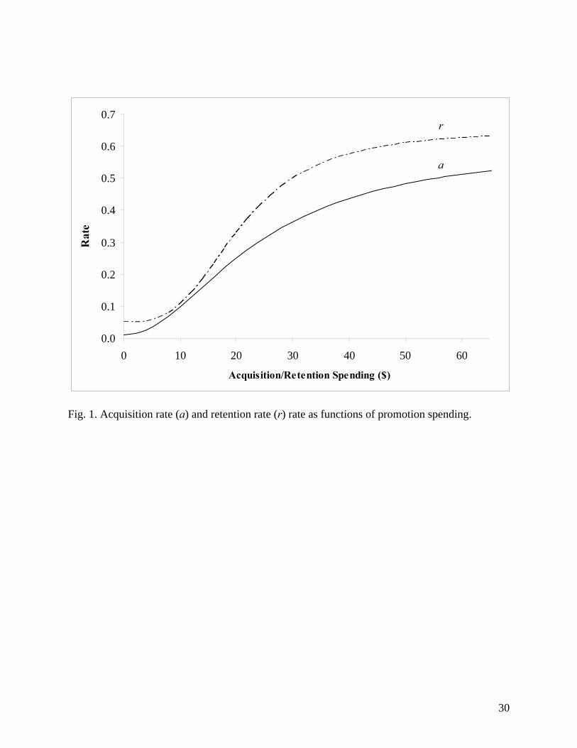
Solving equations (11) and (12) simultaneously, we get = 472.43 and = 1.93. Thus, in this
example, the relationship between acquisition rate and acquisition spending happens to be S-
shaped (since >1; see Figure 1).
1K 1b
1b
12

-------------------------------------------------
Insert Figure 1 about here
-------------------------------------------------
Similarly, assume that when asked about the current retention spending and retention rate, the
manager reports $20 and 33%, respectively. Thus, we have:
33.020
20)05.065.0(05.02
2
220$ =
+−+= b
b
Kr (13)
The manager is also asked to estimate the retention rate if the retention spending per customer
were $10 greater (i.e., $30). Let us say the manager reports 50%. We have:
50.030
30)05.065.0(05.02
2
230$ =
+−+= b
b
Kr (14)
Solving equations (13) and (14) simultaneously, we get = 10,271.23 and = 3.04. Hence,
the retention rate is also S-shaped with retention spending (see Figure 1; see also Table 1 for a
summary of the input values provided by the manager for this example).
2K 2b
-------------------------------------------------
Insert Table 1 about here
-------------------------------------------------
Using the parameter values above, along with the managerial inputs, we proceed to find
the optimal promotion allocation between acquisition and retention using the model defined in
equation (10). Because acquisition and retention spending (i.e., andA R ) are nonlinearly related
to acquisition rate and retention rate (see equations (8) and (9)), the equations generated using an
algebraic (e.g., Lagrangian) approach to solve for an optimal solution are intractable. Thus, we
use numerical optimization procedures and find that the optimal acquisition spending per
prospect (A0 ) is $40.48, optimal retention spending per customer (R0) is $44.44, and maximum
customer equity (CE0) is $275.81. Note that the budget constraint is satisfied since A0 + a0R0 =
13

$40.48 + (0.439)($44.44) = $60, where a0 is the acquisition rate at the optimal acquisition
spending.
6. Determination of optimal channel quality
Note that the optimal allocation strategy and maximum customer equity values calculated
in the previous section are both based on the manager’s currently used promotion channel (i.e., θ
= 6). An important implication of our extended model is that the manager, operating under the
same budget constraint, can obtain even higher customer equity by optimizing on channel quality.
Since channel quality impacts optimal customer equity through its relationships with the ceiling
rates of acquisition and retention, we must obtain additional managerial inputs for equations (4)
and (5) in order to optimize channel quality.
To get the values of the parameter 0α in equation (4), we ask the manager to estimate the
ceiling rate of acquisition if the channel were totally quality-oriented. Assume the manager
provides an answer of 1% (i.e., 0α = 0.01). Using the previously reported ceiling rates for
acquisition (0.60) and retention (0.65), we have:
(15) 60.0601.0 216| =⋅+==
αθ αaC
(16) 65.061 216| =⋅−==
βθ βrC
To acquire an additional point on each ceiling rate curve, we ask the manager to estimate
the ceiling acquisition rate and retention rate if the channel were totally quantity-oriented (i.e., θ
= 10). Assume the manager indicates these rates are 80% and 10%, respectively. We have:
(17) 80.01001.0 2110| =⋅+==
αθ αaC
(18) 10.0101 2110| =⋅−==
βθ βrC
14

Solving equations (15), (16), (17), and (18) simultaneously, we find 1α = 0.2119, 2α = 0.5714,
1β = 0.0127, and 2β =1.8489. Figure 2 illustrates the relationships among , , and θ. aC rC
-------------------------------------------------
Insert Figure 2 about here
-------------------------------------------------
As mentioned before, 1α , 2α , 1β , and 2β are assumed to be constant parameters across
all promotion channels for this particular product. Using these parameter values, equation (10),
and numerical optimization, we find that the optimal channel quality is θ = 2.8. If the manager
opts for a promotion channel with this optimal quality, the optimal budget allocation becomes A
= $41.85 per prospect and R = $62.05 per customer. The new optimal customer equity is $345.00,
an increase of $61.19 (or 21.6%) over that obtained with the currently used channel (i.e., θ = 6).
7. Sensitivity analysis
In this section we provide two distinct kinds of sensitivity analysis. The first examines, in
a traditional sense, the sensitivity of the optimal values of the decision variables and optimal
customer equity to differences in the values of various input parameters. The second, introduced
since we are using decision calculus and the manager’s subjective estimates, is to study the
sensitivity of the optimal customer equity to the inaccuracy of the manager’s inputs.
7.1. Sensitivity analyses for selected parameter values
We first perform a sensitivity analysis with regard to channel quality (θ ). Table 2 shows
that when the promotion channel becomes more quantity-oriented (i.e., channel quality
increases), the optimal acquisition rate (a0) increases while the optimal retention rate (r0)
15

decreases. The values of and in Table 2 also illustrate the role of channel quality in
accounting for this negative relationship. Additionally, Figure 3 depicts the complex relationship
between channel quality and both acquisition and retention spending. Finally, consistent with our
assertions, Table 2 and Figure 3 indicate that there exists an optimal channel quality in customer
equity maximization (as customer equity is ∩-shaped with channel quality.
aC rC
-------------------------------------------------
Insert Table 2 and Figure 3 about here
-------------------------------------------------
We next conduct a sensitivity analysis with regard to preset promotion budget (B), with
the assumption that the manager optimizes the promotion channel (i.e., θ = 2.8). According to
Table 3, holding all else constant, an increased preset promotion budget, not surprisingly, results
in higher optimal acquisition and retention spending. This leads to increased acquisition rate and
retention rate and, therefore, customer equity is increased. For example, when the preset
promotion budget increases from $60 to $80 per prospect, optimal acquisition spending increases
from $41.04 to $56.27 per prospect and optimal retention spending increases from $57.83 to
$63.80 per customer. The optimal customer equity increases from $338.31 to $378.60. However,
notice that the marginal return of optimal customer equity decreases sharply with the preset
promotion budget. For example, when the budget increases from $20 to $30, the customer equity
increases from $121.58 to $193.75 (i.e., increase of $72.17, or 59.4%). However, when the preset
promotion budget increases from $100 to $110, customer equity increases from $392.74 to
$393.91 (i.e., increase of only $1.17, or 0.30%). More importantly, Table 3 reveals that when the
preset promotion budget approaches $110 per prospect, the customer equity no longer increases.
This means that $393.91 per prospect is the highest customer equity the company can obtain for
16

the product, and that presetting the promotion budget for more than $110 per prospect leads only
to wasting resources.
-------------------------------------------------
Insert Table 3 about here
-------------------------------------------------
Lastly, we present a sensitivity analysis for marginal contribution (m). The middle section
of Table 3 shows that, as expected, customer equity goes up as unit marginal contribution
increases. Indeed, for each $100 increase in marginal contribution, optimal customer equity
increases slightly more than $100. However, we can also see from Table 3 that changes in
marginal contribution have little impact on the optimal allocation of the preset promotion budget.
To illustrate, when marginal contribution increases from $200 to $600 per purchase, optimal
acquisition spending only decreases from $42.47 to $40.52 per prospect and the retention
spending only increases from $53.61 to $59.81 per customer.
Finally, we conduct a sensitivity analysis with regard to discount rate (d). The bottom
section of Table 3 indicates that as the discount rate increases, acquisition spending increases
while retention spending decreases. For example, when the discount rate increases from 10% to
30%, optimal acquisition spending increases from $40.04 to $41.72 per prospect while optimal
retention spending decreases from $61.66 to $55.32 per customer. Note that, whereas the optimal
spending pattern changes only moderately (considering the tripling of the discount rate), optimal
customer equity decreases more dramatically (from 433.32 to $285.22, or –34.2%).
7.2. Sensitivity analysis to inaccuracy of selected managerial inputs
Note that in the prototype real-world example above, the inputs from the manager are
based on experience and subjective judgments and, therefore, may be inaccurate. Whereas the
17

preceding sensitivity analysis focuses on the effect of environmental parameters on the optimal
outcomes, the sensitivity analysis in this section examines the effect of inaccuracy in the
managerial inputs on the optimal outcomes.
Recall that the ceiling rates specify the acquisition and retention rates in the case where
spending is unlimited. Thus, of the managerial inputs, we expect managers may have the most
difficulty estimating the ceiling rates of acquisition and retention since these values are the most
remote from the manager’s current situation (Chakravarti and Staelin, 1981). Thus, we conduct
sensitivity analyses with regards to the inaccuracy of Ca and Cr, as estimated by the manager for
the current channel quality (i.e., and 6| =θaC | 6rC θ = ), assuming all other inputs are accurate.
If the true values of and | 6aC θ = | 6rC θ = are different from the values the manager reports,
the parameters defined in equations (4), (5), (8), and (9) take on different values. Thus, the
optimal outcomes from the model will be changed, and, indeed, will be non-optimal. We begin
with Table 4, which shows how the optimal results change with varying true values of | 6aC θ = and
. To recall, the manager’s inputs indicate that | 6rC θ = | 6aC θ = = 0.60 and | 6rC θ = = 0.65. Assuming
these are the correct values, the model indicates that optimal channel quality is θ = 2.8, optimal
acquisition and retention spending are $41.85 per prospect and $62.05 per customer, respectively,
and optimal customer equity is $345.00. However, if, for example, | 6aC θ = = 0.55 and | 6rC θ = = 0.60
are the true ceiling rates at θ = 6, the model would indicate that the optimal channel quality is
actually θ = 3.4 (with optimal acquisition spending and retention spending of $44.39 per
prospect and $52.34 per customer, respectively). The optimal customer equity drops to $280.66.
Table 4 provides optimal values for other combinations of | 6aC θ = and | 6rC θ = .
18
-------------------------------------------------
Insert Table 4 about here
-------------------------------------------------
Note that, holding constant and allowing | 6rC θ = | 6aC θ = to increase, we observe an
increasing optimal customer equity and a decreasing optimal channel quality. This is consistent
with our expectation, because an increasing | 6aC θ = indicates an improved market environment and
the potential to obtain, by whatever change in promotion budget allocation is optimally indicated,
a higher customer equity. A similar observation can be made with regard to an increasing | 6rC θ = .
We now examine the sensitivity of the model to inaccuracy in the manager’s ceiling rate
estimates for the currently used channel. In this example, | 6aC θ = = 0.60 and = 0.65 are the
values reported by the manager, which may or may not be the true values. The manager will
observe the output of the model and choose channel quality θ = 2.8, spend $41.85 per prospect
in acquisition and $62.05 per customer in retention, and anticipate customer equity of $345.00.
However, the maximum realized customer equity will be different, if the true ceiling rates are
not as assumed. Table 5 reveals the respective customer equity values when the model uses
= 0.60 and = 0.65, while the true values of
| 6rC θ =
| 6aC θ = | 6rC θ = | 6aC θ = and | 6rC θ = are the corresponding
row and column designations.
-------------------------------------------------
Insert Table 5 about here
-------------------------------------------------
Naturally, the suboptimal customer equities in Table 5 are smaller than their optimal cell-
by-cell counterparts in Table 4, except for the middle cell, in which the manager’s estimates are
accurate. Table 5 also presents the percentage differences between the suboptimal customer
19

equities and the corresponding optimal customer equities. In a sense, the percentage decreases
represent the “punishment” for the inaccurate managerial inputs. For example, if the true values
of and are 0.55 and 0.70, respectively, the optimal customer equity is $313.52, while
the suboptimal customer equity is $291.46. Thus, the manager is “punished” by $22.06 (or
7.04%) for inaccurate assessments of the ceiling rates and subsequent implementation of a
promotion budget allocation strategy corresponding to these inaccurate assessments.
| 6aC θ = | 6rC θ =
Two other points in Table 5 are noteworthy. First, errors by the manager in estimating Ca
and Cr in this example do not tend to “cancel out.” When estimation inaccuracy in Ca and Cr
occurs simultaneously (in either the same or opposite direction), the suboptimal customer equity
is significantly smaller than its counterpart based on the true values of and . Second,
the magnitudes of the percentage deviations in Table 5 are large enough to justify an
optimization procedure (especially for larger target markets) but small enough so that the optimal
solution is not overly sensitive to the manager’s estimation errors.
| 6aC θ = | 6rC θ =
8. Discussion and limitations
In this paper, we extended the literature on customer equity optimization and optimal
allocation of promotion budget spending (e.g., Berger and Nasr, 1998; Berger and Nasr-
Bechwati, 2001; Blattberg and Deighton, 1996) in several ways. Specifically, we motivated
channel quality as a relevant decision variable, explicated its role in the model, and demonstrated
the existence of an optimal value. In addition, we relaxed the general concavity assumption
between acquisition (retention) rate and acquisition (retention) spending by introducing the
ADBUDG function (Little, 1970). This function does not mandate whether the acquisition
(retention) response curve is concave or S-shaped. Rather, it allows the manager’s specific, real-
20

world situation to determine which shape is appropriate. Lastly, we removed the restriction
embodied in previous models that zero expenditure on acquisition (retention) results in a zero
acquisition (retention) rate.
After presenting an extended model, we demonstrated how to apply it by providing a
prototype real-world example in which the decision calculus approach was used to estimate the
model parameters. Also, we performed two types of sensitivity analyses. The first type of
sensitivity analysis focused on how sensitive the optimal outcomes from the model are to the
values of certain input parameters. The second type of sensitivity analysis illustrated how the
optimal model outcomes are impacted by inaccuracy in the managerial inputs.
Our study, as any study, has limitations. The objective function in the model presumes
that a vendor applies the same promotion channel in each purchase season and that customers
make a purchase, if they are retained, only once during each purchase season. Additionally, the
model only considers a one-company-one market case. More realistic is the case that, in each
market segment, several companies may be competing with various products that may provide
similar or complementary functions and benefits. These assumptions are, for the most part,
shared by previous work (e.g., Berger and Nasr-Bechwati 2001). However, the model presented
here should be able to accommodate a relaxation of nearly all of these assumptions.
21

References
Aaker, DA, and Carman, JM. Are You Over-Advertising? Journal of Advertising Research 1982;
22(4): 57-70. Berger, PD, and Nasr, NI. Marketing Models and Applications. Journal of Interactive Marketing
1988; 12(1): 17-30. Berger, PD, and Nasr-Bechwati, N. The Allocation of Promotion Budget to Maximize Customer
Equity. OMEGA: The International Journal of Management Science 2001; 29(1): 49-61. Blattberg, R, and Deighton, J. Manage Marketing by the Customer Equity Test. Harvard
Business Review 1996; 74(4): 136-144. Blattberg, RC, Getz, G, and Thomas, J. Customer Equity – Building and Managing Customer
Relationships as Valuable Assets. Boston: Harvard Business School Press, 2001. Bolton, RN, Lemon, KN, and Verhoef, PC. The Theoretical Underpinnings of Customer Asset
Management: A Framework and Propositions for Future Research. Journal of the Academy of Marketing Science 2004; 32(3): 271-292.
Chakravarti, D, Mitchell, A, and Staelin, R. Judgment Based Marketing Decision Models:
Problems and Possible Solutions. Journal of Marketing 1981; 45(3): 13-23. Desai, KK, and Mahajan V. Strategic Role of Affect-Based Attitudes in the Acquisition,
Development, and Retention of Customers. Journal of Business Research 1998; 42: 309-324. Dorsch, MJ, and Carlson, LA. Transaction Approach to Understanding and Managing Customer
Equity. Journal of Business Research 1996; 35: 253-264. Dwyer, FR. Customer Lifetime Valuation to Support Marketing Decision Making. Journal of
Direct Marketing 1997, 11(4); 6-13. Fam, KS, and Yang, Z. Primary Influences of Environmental Uncertainty on Promotions Budget
Allocation and Performance: A Cross-Country Study of Retail Advertisers. Journal of Business Research 2006; 59: 259-267.
Gounaris, SP. Trust and Commitment Influences on Customer Retention: Insights from
Business-to-Business Services. Journal of Business Research 2005; 58: 126-140. Hogan, JE, Lemon, K, and Libai, B. Quantifying the Ripple: Word-of-Mouth and Advertising
Effectiveness. Journal of Advertising Research 2004; 44(3): 271-280. Jackson, B. Winning and Keeping Industrial Customers. Lexington, MA: Lexington Books, 1985.
22

Johansson, JK. Advertising and the S-Curve: A New Approach. Journal of Marketing Research 1979; 16(3): 345-354.
Jones, E, Busch, P, and Dacin, P. Firm Market Orientation and Salesperson Customer
Orientation: Interpersonal and Intrapersonal Influences on Customer Service and Retention in Business-to-Business Buyer-Seller Relationships. Journal of Business Research 2003; 56: 323-340.
Kumar, V, Ramani, G, and Bohling, T. Customer Lifetime Value Approaches and Best Practice
Applications. Journal of Interactive Marketing 2004; 18(3): 60-72. Little, JDC. Models and Managers: the Concept of a Decision Calculus. Management Science
1970; 16(8): 466-484. Little, JDC. BRANDAID: A marketing-mix model, part 1: Structure. Operations Research 1975;
23: 628-655. Little, JDC. Aggregate Advertising Models: the State of the Art. Operations Research 1979;
27(4): 629-66. Lodish, LM, Curtis, E, Ness, M, and Simpson, MK. Sales Force Sizing and Deployment Using a
Decision Calculus Model at Syntex Laboratories. Interfaces 1988; 18(1): 5-20. Neslin, S, Grewal, D, Leghorn, R, Shankar, V, Teerling, M, Thomas, J, and Verhoef, P.
Challenges and Opportunities in Multichannel Customer Management. forthcoming, Journal of Services Marketing 2006.
Pfeifer, P, and Carraway, RL. Modeling Customer Relationships as Markov Chains. Journal of
Interactive Marketing 2000; 14(2): 43-55. Rao, AG, and Miller, PB. Advertising/Sales Response Functions. Journal of Advertising
Research 1975; 15(2): 7-15. Ray, ML, and Sawyer, AG. Repetition in Media Models: A Laboratory Technique. Journal of
Marketing Research 1971; 8(1): 20-29. Reinartz, W, Thomas, JS, and Kumar, V. Balancing Acquisition and Retention Resources to
Maximize Customer Profitability. Journal of Marketing 2005; 69(1): 63-79. Rust, RT, Lemon, KN, and Zeithaml, V. Return on Marketing: Using Customer Equity to Focus
Marketing Strategy. Journal of Marketing 2004; 68(1): 109-127. Simon, JL, and Arndt, J. The Shape of the Advertising Response Function. Journal of
Advertising Research 1980; 20(4): 11-28. Stigler, GJ. The Economics of Information. Journal of Political Economy 1961; 69(3): 213-225.
23

Thomas, JS. A Methodology for Linking Customer Acquisition to Customer Retention. Journal
of Marketing Research 2001; 38(2): 262-268. van Bruggen, GH, Smidts, A, and Wierenga, B. The Powerful Triangle of Marketing Data,
Managerial Judgment, and Marketing Management Support Systems. European Journal of Marketing 2001; 35(7): 796–814.
Venkatesan, R, and Kumar, V. A Customer Lifetime Value Framework for Customer Selection
and Resource Allocation Strategy. Journal of Marketing 2004; 68(4): 106-125. Verhoef, PC, and Donkers, B. The Effect of Acquisition Channels on Customer Loyalty and
Cross-buying. Journal of Interactive Marketing 2005; 19(2): 31-43. Villanueva, J, Yoo, S, and Hanssens, D. The Impact of Marketing-Induced vs. Word-of-Mouth
Customer Acquisition on Customer Equity. Working paper No. 516: IESE Business School, University of Navarra, 2006.
Wang, P, and Spiegel, T. Database marketing and Its Measurements of Success: Designing a
Managerial Instrument to Calculate the Value of a Repeat Customer Base. Journal of Direct Marketing 1994; 8(2): 73-81.
24

Table 1 Manager’s inputs to the extended model
Inputs Requested from Manager Parameter Manager’s Estimate
1. Size of the target market 1,000,000 2. Promotion budget allocated to the target market (1,000,000)·B $60,000,000 3. Yearly contribution margin per customer m $400 4. Yearly discount rate d 20% 5. Quality of the currently used promotion channel θ 6 6. Amount spent per prospect for the purpose of acquisition A $10 7. Amount spent per new customer for the purpose of retention R $20 8. Percentage of prospects the current promotion channel could
have acquired if acquisition spending were unlimited Ca|θ=6 60%
9. Percentage of prospects the current promotion channel could have acquired if there were no spending on acquisition
a0 1%
10. Percentage of new customers that would have been retained if retention spending were unlimited
Cr|θ=6 65%
11. Percentage of new customers that would have been retained if there were no spending on retention
r0 5%
12. Percentage of prospects purchasing product in past year a$10 10% 13. Percentage of prospects that would have purchased product if
acquisition spending per prospect had been $10 higher a$20 25%
14. Percentage of new customers that have been retained r$20 33% 15. Percentage of new customers that would have been retained if
the retention spending per new customer had been $10 higher r$30 50%
16. Percentage of prospects a totally quantity-oriented channel would have acquired if acquisition spending were unlimited
Ca|θ=10 80%
17. Percentage of new customers a totally quantity-oriented channel would have retained if retention spending were unlimited
Cr|θ=10 10%
25
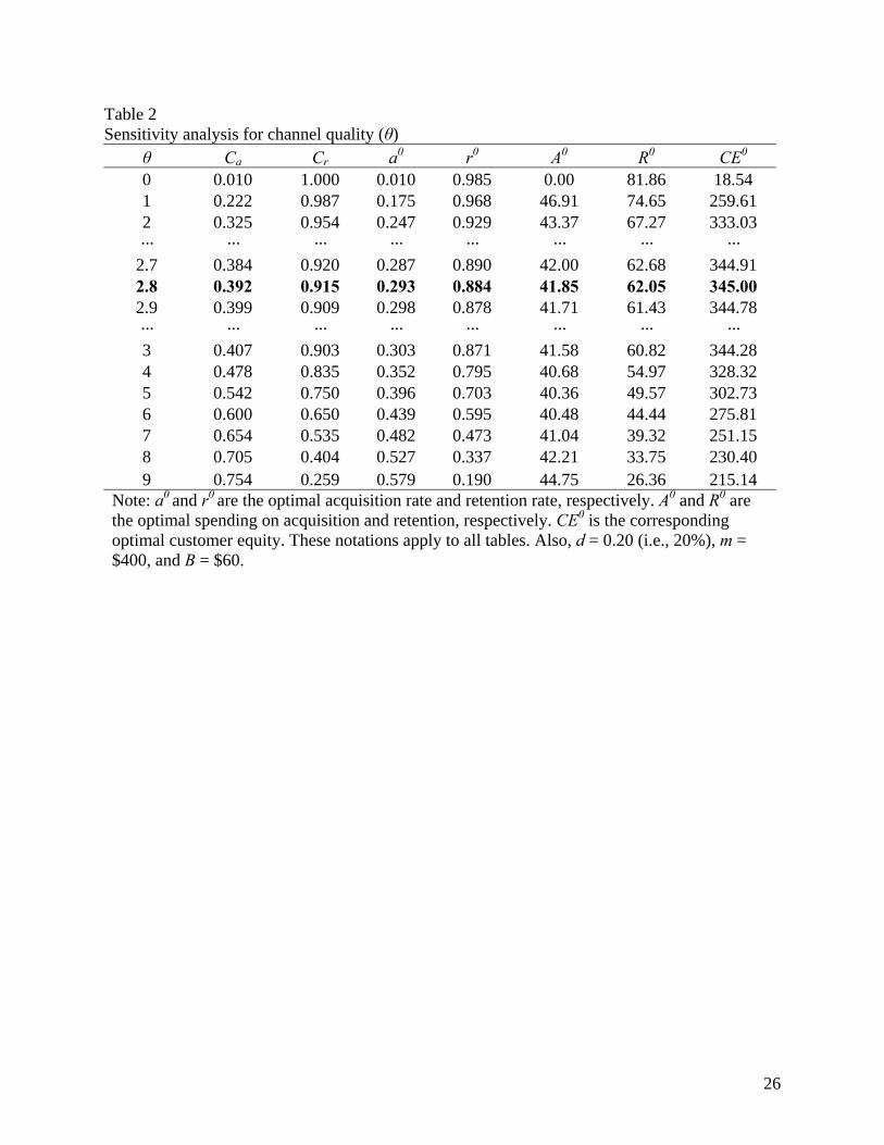
Table 2 Sensitivity analysis for channel quality (θ)
θ Ca Cr a0 r0 A0 R0 CE0 0 0.010 1.000 0.010 0.985 0.00 81.86 18.54 1 0.222 0.987 0.175 0.968 46.91 74.65 259.61 2 0.325 0.954 0.247 0.929 43.37 67.27 333.03 ··· ··· ··· ··· ··· ··· ··· ··· 2.7 0.384 0.920 0.287 0.890 42.00 62.68 344.91 2.8 0.392 0.915 0.293 0.884 41.85 62.05 345.00 2.9 0.399 0.909 0.298 0.878 41.71 61.43 344.78 ··· ··· ··· ··· ··· ··· ··· ··· 3 0.407 0.903 0.303 0.871 41.58 60.82 344.28 4 0.478 0.835 0.352 0.795 40.68 54.97 328.32 5 0.542 0.750 0.396 0.703 40.36 49.57 302.73 6 0.600 0.650 0.439 0.595 40.48 44.44 275.81 7 0.654 0.535 0.482 0.473 41.04 39.32 251.15 8 0.705 0.404 0.527 0.337 42.21 33.75 230.40 9 0.754 0.259 0.579 0.190 44.75 26.36 215.14
Note: a0 and r0 are the optimal acquisition rate and retention rate, respectively. A0 and R0 are the optimal spending on acquisition and retention, respectively. CE0 is the corresponding optimal customer equity. These notations apply to all tables. Also, d = 0.20 (i.e., 20%), m = $400, and B = $60.
26

Table 3 Sensitivity to preset budget (B), marginal contribution (m), and discount rate (d)
Parameter Value a0 r0 A0 R0 CE0 ∆CE 20 0.122 0.810 14.12 48.07 121.58 30 0.192 0.815 20.54 49.31 193.75 72.17 40 0.249 0.822 27.10 51.72 255.19 61.44 50 0.294 0.829 33.92 54.68 303.15 47.96 60 0.328 0.835 41.04 57.83 338.31 35.16 70 0.353 0.840 48.49 60.92 362.70 24.39 80 0.372 0.844 56.27 63.80 378.60 15.90 90 0.386 0.847 64.38 66.35 388.06 9.47 100 0.397 0.849 72.80 68.53 392.74 4.68 110 0.405 0.851 80.55 70.17 393.91 1.17
B
120 0.405 0.851 80.55 70.17 393.91 0.00 200 0.333 0.824 42.47 52.61 123.65 300 0.330 0.832 41.54 55.97 230.65 107.00 400 0.328 0.835 41.04 57.83 338.31 107.66 500 0.327 0.837 40.73 59.00 446.24 107.93
m
600 0.326 0.839 40.52 59.81 554.32 108.07 10% 0.324 0.841 40.04 61.66 433.32 15% 0.326 0.838 40.60 59.51 377.94 -55.38 20% 0.328 0.835 41.04 57.83 338.31 -39.63 25% 0.329 0.833 41.41 56.46 308.49 -29.82
d
30% 0.331 0.830 41.72 55.32 285.22 -23.28 Note: Unless parameter value is varied for purpose of sensitivity analysis,θ = 2.8, B= $60, d = 0.20 (i.e., 20%), and m = $400.
27

Table 4 Sensitivity analysis for changes in | 6rC θ = and | 6aC θ =
| 6aC θ = = 0.55 | 6aC θ = = 0.60 | 6aC θ = = 0.65A0 44.39 44.30 43.40 R0 52.34 54.44 54.84
CE0 280.66 330.74 398.26 | 6rC θ = =0.60
θ0 3.4 2.6 2.0 A0 42.25 41.85 40.96 R0 60.69 62.05 62.43
CE0 298.15 345.00 404.59 | 6rC θ = = 0.65
θ0 3.5 2.8 2.2 A0 40.06 39.69 38.76 R0 67.07 68.63 68.30
CE0 313.52 355.49 406.34 | 6rC θ = = 0.70
θ0 3.7 3.0 2.5 Note: A0, R0, and CE0 are based on their corresponding optimal channel quality, θ0.
28

Table 5 Sensitivity of suboptimal customer equity (CEsub) to changes in | 6rC θ = and | 6aC θ =
| 6aC θ = = 0.55 | 6aC θ = = 0.60 | 6aC θ = = 0.65
CE0 CEsub ∆CE CE0 CEsub ∆CE CE0 CEsub ∆CE
| 6rC θ = =0.60 280.66 270.15 -3.75% 330.74 326.01 -1.43% 398.26 382.49 -3.96%| 6rC θ = = 0.65 298.15 286.25 -3.99% 345.00 345.00 0.00% 404.59 393.78 -2.67%| 6rC θ = = 0.70 313.52 291.46 -7.04% 355.49 351.14 -1.22% 406.34 390.72 -3.85%
Note: Customer equities calculated with A = $41.85, R = $62.05, and θ = 2.8, unless suboptimal allocation lead to violation of the budget constraint (in which case R is reduced accordingly). Percentages represent (CEsub –CE0)/CE0, where CE0 is reproduced from Table 4 for convenience.
29
0.0
0.1
0.2
0.3
0.4
0.5
0.6
0.7
0 10 20 30 40 50 60
Acquisition/Retention Spending ($)
Rat
e
r
a
Fig. 1. Acquisition rate (a) and retention rate (r) rate as functions of promotion spending.
30

0.0
0.1
0.2
0.3
0.4
0.5
0.6
0.7
0.8
0.9
1.0
0 1 2 3 4 5 6 7 8 9 10
Channel Quality (θ )
Rat
e
Ca
Cr
Fig. 2. Acquisition ceiling rate (Ca) and retention ceiling rate (Cr) as functions of channel quality (θ ).
31

0
10
20
30
40
50
60
70
80
90
0 1 2 3 4 5 6 7 8 9 10
Channel Quality (θ )
Acq
uisit
ion/
Ret
entio
n Sp
endi
ng ($
)
0
50
100
150
200
250
300
350
400
Cus
tom
er E
quity
($)
CE0
R0
A0
Fig. 3. Optimal acquisition spending (A0), retention spending (R0), and customer equity (CE0) as functions of channel quality (θ ).
32
Related Documents


