The Iby and Aladar Fleischman Faculty of Engineering The Zandman-Slaner School of Graduate Studies The Department of Electrical Engineering - Systems The Robustness of Dirty Paper Coding and The Binary Dirty Multiple Access Channel with Common Interference Thesis submitted toward the degree of Master of Science in Electrical and Electronic Engineering by Anatoly Khina April, 2010

Welcome message from author
This document is posted to help you gain knowledge. Please leave a comment to let me know what you think about it! Share it to your friends and learn new things together.
Transcript
The Iby and Aladar Fleischman Faculty of Engineering
The Zandman-Slaner School of Graduate StudiesThe Department of Electrical Engineering - Systems
The Robustness ofDirty Paper Coding
andThe Binary Dirty
Multiple Access Channelwith Common Interference
Thesis submitted toward the degree of
Master of Science in Electrical and Electronic Engineering
by
Anatoly Khina
April, 2010

The Iby and Aladar Fleischman Faculty of Engineering
The Zandman-Slaner School of Graduate StudiesThe Department of Electrical Engineering - Systems
The Robustness ofDirty Paper Coding
andThe Binary Dirty
Multiple Access Channelwith Common Interference
Thesis submitted toward the degree of
Master of Science in Electrical and Electronic Engineering
by
Anatoly Khina
This research was carried out at the
Department of Electrical Engineering - Systems,Tel-Aviv University
Advisor:Dr. Uri Erez
April, 2010


“The least initial deviation from the truth
is multiplied later a thousandfold.”
Aristotle
Acknowledgements
I wish to express my utmost appreciation and gratitude to Dr. Uri Erez,
who took me under his wing as a third year undergraduate student, and helped
me making my first steps in the exciting, and to me, new world of information
theory and communication. For his professional guidance and dedicated super-
vising, which shaped the way I approach and handle new theoretical problems.
And for his patience and invaluable advice.
I thank Prof. Ram Zamir for serving as a true “academic grandfather” to
me. I first met Rami in the undergraduate course “random signals and noise”,
which fascinated me and convinced me to pursue in this direction. Later on, his
advanced information theory course gave me most of the basic tools I needed
as a young researcher in the area of information theory, at the end of which I
was able to conduct my research.
In the course of this work, I had the privilege of working together with Yuval
Kochman and Tal Philosof on things within and outside the scope of this work.
Yuval always sees things in a unique way, which frequently makes things look
much simpler and their solutions - “natural”. Tal has a broad vision and vast
knowledge and understanding of both, theoretical and practical, aspects of
communication systems. I learned a lot from both of them and for that I am
grateful.
I would like to thank my other colleagues from 102 and 108 labs, as well,
who made this period enjoyable and full of interesting interactions, both in
academic and non-academic issues: Amir Alfandary, Ohad Barak, Ohad Ben-
Cohen, Idan Goldenberg, Eli Haim, Amir Ingber, Roy Jevnisek, Oron Levy,
Yuval Lomnitz, Eado Meron, Noam Presman, Ofer Shayevitz, Mikhal Shemer,
Alba Sloin, Nir Weinberger, Yair Yona and Pia Zobel.
I would like to acknowledge the support of the Israeli ministry of trade and
commerce as part of Nehusha/iSMART project and the Yitzhak and Chaya
Weinstein Research Institute for Signal Processing at Tel Aviv University.
Finally warm thanks to my parents Tatyana and Alexander, for their end-
less support and caring.


Abstract
A dirty-paper channel is considered, where the transmitter knows the inter-
ference sequence up to a constant multiplicative factor, known only to the
receiver. Lower bounds on the achievable rate of communication are derived
by proposing a coding scheme that partially compensates for the imprecise
channel knowledge. We focus on a communication scenario where the signal-
to-noise ratio is high. Our approach is based on analyzing the performance
achievable using lattice-based coding schemes. When the power of the inter-
ference is finite, we show that the achievable rate of this lattice-based coding
scheme may be improved by a judicious choice of the scaling parameter at the
receiver. We further show that the communication rate may be improved, for
finite as well as infinite interference power, by allowing randomized scaling at
the transmitter. This scheme and its analysis are used to compare the per-
formance of linear and dirty paper coding transmission techniques over the
MIMO broadcast channel, in the presence of channel uncertainty.
We also consider a binary dirty multiple-access channel with interference
known at both encoders. We derive an achievable rate region for this channel
which contains the sum-rate capacity and observe that the sum-rate capacity
in this setup coincides with the capacity of the channel when full-cooperation
is allowed between transmitters, contrary to the analogous Gaussian case.


Nomenclature
AWGN Additive White Gaussian Noise
BC Broadcast
BSC Binary Symmetric Channel
DMAC Dirty Multiple-Access Channel
DMC Discrete Memoryless Channel
DP Dirty Paper
DPC Dirty Paper Coding
MAC Multiple-Access Channel
MIMO Multiple-Input Multiple-Output
MMSE Minimum Mean-Square Error
MSE Mean-Square Error
SI Side Information
SIR Signal-to-Interference Ratio
SNR Signal-to-Noise Ratio
THP Tomlinson-Harashima Precoding
ZF Zero-Forcing
a vector
an1 a1, ..., an
||a|| The L2-norm of a
X Random variable
X The alphabet of the random variable X
|X | The Cardinality of the alphabet XX Random vector
p(x) Probability density function
p(x, y) Joint probability density function
p(y|x) Conditional probability density function
iii

iv
EX The expectation of X
Bernoulli(p) Bernoulli distribution with parameter p
Unif (R) Uniform distribution over region RN (μ, σ2) Gaussian distribution with expectation μ and variance σ2
H(X) The entropy of a discrete random variable X
h(X) The differential entropy of a continuous random variable X
Hb(p) The entropy of a binary random variable X ∼ Bernoulli(p)
H+b (p) Hb
(min
{p, 1
2
})I(X;Y ) The mutual information of two random variables X, Y
cl conv{R} Closure and Convex hull of the region Ru.c.e{f(x)} The upper convex envelope of f(x) w.r.t x
⊕ Modulo-two addition
wH Hamming weight
R The set of real numbers
Z The set of integer numbers
Z2 Galois field of size 2
mod 2 modulo-2 operation
mod Λ modulo lattice Λ operation
q1 � q2 (1 − q1)q2 + q1(1 − q2)
|| · || Euclidean norm
〈·, ·〉 Euclidean inner-product
csc(x) 1/ sin(x)
sec(x) 1/ cos(x)
Contents
1 Introduction 1
1.1 Dirty Paper Coding Robustness . . . . . . . . . . . . . . . . . . 1
1.2 Binary Dirty MAC with Common Interference . . . . . . . . . . 4
1.3 Thesis Organization . . . . . . . . . . . . . . . . . . . . . . . . . 5
1.4 Background . . . . . . . . . . . . . . . . . . . . . . . . . . . . . 6
1.4.1 Channels with SI at Tx . . . . . . . . . . . . . . . . . . . 6
1.4.2 Writing on Dirty Paper . . . . . . . . . . . . . . . . . . . 7
1.4.3 Lattice-Strategies . . . . . . . . . . . . . . . . . . . . . . 10
1.4.4 Compound Channels . . . . . . . . . . . . . . . . . . . . 14
1.4.5 Compound Channels With SI at Tx . . . . . . . . . . . . 14
1.4.6 Gaussian MIMO Broadcast Channels . . . . . . . . . . . 15
1.4.7 Multiple-Access Channel . . . . . . . . . . . . . . . . . . 20
1.4.8 Dirty Multiple-Access Channel . . . . . . . . . . . . . . . 21
2 Robustness of Dirty Paper Coding 24
2.1 Channel Model and Motivation . . . . . . . . . . . . . . . . . . 25
2.2 Compound Channels with Causal SI at Tx . . . . . . . . . . . . 26
2.3 Compensation for Channel Uncertainty at Tx . . . . . . . . . . 27
2.3.1 THP With Imprecise Channel Knowledge . . . . . . . . 27
2.3.2 Naıve Approach . . . . . . . . . . . . . . . . . . . . . . . 30
2.3.3 Smart Receiver - Ignorant Transmitter . . . . . . . . . . 30
2.3.4 High SNR Regime . . . . . . . . . . . . . . . . . . . . . 32
2.4 Randomized Scaling at Transmitter . . . . . . . . . . . . . . . . 34
2.4.1 Quantifying the Achievable Rates . . . . . . . . . . . . . 36
2.4.2 Upper Bound on Achievable Rates . . . . . . . . . . . . 38
2.4.3 Noisy Case . . . . . . . . . . . . . . . . . . . . . . . . . 39
v
vi CONTENTS
2.5 Non-Causal Case and Multi-Dimensional Lattices . . . . . . . . 40
2.6 Implications to MIMO BC Channels . . . . . . . . . . . . . . . 41
2.6.1 Linear Zero-Forcing . . . . . . . . . . . . . . . . . . . . . 41
2.6.2 Dirty Paper Coding . . . . . . . . . . . . . . . . . . . . . 43
3 Binary Dirty Multiple-Access Channel 49
3.1 System Model and Motivation . . . . . . . . . . . . . . . . . . . 49
3.2 Clean MAC . . . . . . . . . . . . . . . . . . . . . . . . . . . . . 50
3.2.1 Onion Peeling . . . . . . . . . . . . . . . . . . . . . . . . 53
3.2.2 Improving the Stationary Onion Peeling . . . . . . . . . 54
3.3 Dirty MAC with Common Interference . . . . . . . . . . . . . . 55
3.3.1 Sum-Rate Capacity . . . . . . . . . . . . . . . . . . . . . 55
3.3.2 Onion Peeling . . . . . . . . . . . . . . . . . . . . . . . . 56
3.3.3 Improved Onion Peeling . . . . . . . . . . . . . . . . . . 57
4 Summary 60
A 62
A.1 Proof of Theorem 2.1 . . . . . . . . . . . . . . . . . . . . . . . . 62
A.2 Proof of Lemma 2.2 and treatment for Δ > 1/3 . . . . . . . . . 63

List of Figures
1.1 DMC with side information at the transmitter . . . . . . . . . . 7
1.2 Dirty paper channel. . . . . . . . . . . . . . . . . . . . . . . . . 8
1.3 Lattice-strategies transmission scheme. . . . . . . . . . . . . . . 12
1.4 Compound DMC . . . . . . . . . . . . . . . . . . . . . . . . . . 14
1.5 Compound DMC with side information at the transmitter . . . 15
1.6 Pictorial representation of ZF for MIMO BC . . . . . . . . . . . 17
1.7 Pictorial representation of DPC in MIMO BC . . . . . . . . . . 19
1.8 Dirty MAC with common state information. . . . . . . . . . . . 22
2.1 Compound dirty-paper channel . . . . . . . . . . . . . . . . . . 25
2.2 SNReff comparison between naıve and smart Rx . . . . . . . . . 31
2.3 Achievable rates and UB on THP . . . . . . . . . . . . . . . . . 37
2.4 Achievable rates of THP for SNR = 17dB . . . . . . . . . . . . 40
2.5 Pictorial representation of ZF in MIMO BCC . . . . . . . . . . 42
2.6 Pictorial representation of DPC for MIMO BCC . . . . . . . . . 44
3.1 Rate Regions for binary DMAC . . . . . . . . . . . . . . . . . . 53
3.2 Rate regions for binary DMAC . . . . . . . . . . . . . . . . . . 58
vii


Chapter 1
Introduction
1.1 Dirty Paper Coding Robustness
The dirty-paper (DP) channel, first introduced by Costa [11], provides an in-
formation theoretic framework for the study of interference cancellation tech-
niques for interference known to the transmitter. The DP channel model has
since been further studied and applied to different communication scenarios
such as ISI channels (see, e.g., [30]), the MIMO Gaussian broadcast chan-
nel [6, 51, 40, 46] and information embedding [2]. The DP model, given by,
Y = X + S +N , (1.1)
is composed of an input signal X, subject to a power constraint, corrupted by
additive white Gaussian noise (AWGN) N and additive interference S which
is known to the transmitter but not to the receiver, causally (“causal DP”)
xi = φ(w, s0, ..., si) ,
or non-causally (“non-causal DP”)
xi = φ(w, s1, ..., sn) ,
where w is the transmitted message, φ is a function satisfying the input con-
straint and xi and si are the channel input and interference at time instance i
(1 ≤ i ≤ n), respectively.
1

2 CHAPTER 1. INTRODUCTION
Costa [11] showed that, for an i.i.d. Gaussian interference with arbi-
trary power, the capacity in the non-causal scenario is equal to that of the
interference-free AWGN channel. This result was extended in [9] to the case
of general ergodic interference and to arbitrary interference in [17].
The capacity of the DP channel with causal knowledge of the interference,
first considered by Willems [47], is not known but upper and lower bounds for
the case of arbitrary interference were found in [17], which coincide in the high
SNR regime, thus establishing the capacity for this case to be the same as for
the interference-free AWGN channel (or equivalently for the non-causal DP
channel) up to a shaping loss. Thus, causality incurs a rate loss of 12log(2πe
12),
relative to the capacity of the interference-free AWGN channel, in the high
SNR regime. This result implies that in the limit of strong interference and
high SNR, the well-known Tomlinson-Harashima precoding (THP) technique
[45, 22] is optimal. For general SNRs, the lattice-based coding techniques of [7,
15, 17] are an extension of Tomlinson-Harashima precoding, sometimes referred
to as MMSE (minimum mean-square error) Tomlinson-Harashima precoding,
where a scaling parameter is introduced at the transmitter and receiver. In this
thesis the term Tomlinson-Harashima precoding is used in this wider sense.
The causal and non-causal DP channels are special cases of the problem
of a general state-dependent memoryless channel. This problem was first in-
troduced by Shannon in 1958 [42], who found the capacity for the case of a
causally known state. Kuznetzov and Tsybakov considered the non-causal sce-
nario [29], the general capacity of which was found by Gel’fand and Pinsker in
1980 [19].
We further note that these channels model communication scenarios where
the channel (i.e., all channel coefficients) is known perfectly to both, the trans-
mitter and the receiver.
In this thesis we focus our attention on scalar precoding, both since it re-
sults in simpler coding schemes but also since the benefit of using a vector
approach (at least using the methods we study) diminishes in the presence of
imprecise channel knowledge, as will be shown in the sequel. Note that scalar
precoding is applicable when the interference is known causally (“Shannon sce-
nario”), whereas vector approaches require non-causal knowledge (“Ge’fand-
Pinsker scenario”). See, e.g., [17].
In many cases of interest, the transmitter has imprecise channel knowledge.
1.1. DIRTY PAPER CODING ROBUSTNESS 3
For instance in a multi-user broadcast scenario, the interference sequence S
corresponds to the signal intended to another user multiplied by a channel
gain. While the transmitter knows the transmitted interfering signal, only an
estimate of the channel gain is known (for instance by quantized feedback; see,
e.g., [24]). This leads to the question, studied in this work, of how sensitive
dirty paper coding (DPC) is to imprecise channel knowledge. We address
this question by adapting the extended Tomlinson-Harashima precoding, as
presented in [17], to the case of imprecise channel knowledge. We consider the
real channel case; for treatment of the case of imperfect phase knowledge, in
the complex channel case, see [21, 3].
Caire and Shamai [6] and Weingarten, Steinberg and Shamai [46] showed
that the private-message capacity of the Gaussian MIMO broadcast (BC) chan-
nel can be achieved using DPC. Nonetheless, it has been speculated in some
works, e.g., [50, 8, 5], that DPC has a significant drawback in the presence of
channel estimation errors, compared to linear approaches such as linear ZF.
In this work, we analyze the performance of both linear ZF and DPC for the
2-user MIMO BC channel and observe that such claims are unqualified.
For the performance analysis of this scheme, we note that the DP channel
with imprecise channel knowledge problem is a special case of the compound
channel with side information at the transmitter problem, first introduced by
Mitran, Devroye and Tarokh [33], which generalizes both the state-dependent
memoryless channel problem and the compound channel problem, considered
in several works [4, 14, 48]. Mitran, Devroye and Tarokh considered the non-
causal scenario, for which they were able to derive upper and lower bounds,
following the steps of Gel’fand-Pinsker [19] and adjusting their proof to the
compound case. Nevertheless, the lower and upper bounds of [33] do not
coincide in general, and the capacity for the non-causal case is yet to be de-
termined. Since, we focus mainly on the causal DP scenario, we consider the
problem of the compound channel with side information known causally at the
transmitter, and derive its capacity, by adjusting the proof by Shannon [42] to
the compound case.

4 CHAPTER 1. INTRODUCTION
1.2 Binary Dirty MAC with Common Inter-
ference
One possible scenario, which generalizes the point-to-point channel with side
information (SI) at the transmitter [42, 19] (and the classical multiple-access
channel (MAC) [1, 32]), is the state-dependent multiple-access channel (MAC).
An important special case of this problem, called the “dirty” MAC in [34]
(after Costa’s “Writing on Dirty Paper” [11]), is the MAC with additive mes-
sages, interference and noise, where different parts of the interference are
known to different users causally or non-causally. Interestingly, the dirty MAC
(DMAC) appears to be a bottleneck in many wireless networks, ad hoc net-
works and relay problems.
Different efforts towards determining the capacity region of the DMAC
were made. In [43, 23], extensions are derived for the achievable of Gel’fand-
Pinsker [19] to the case of state-dependent MAC with different SI availability
scenarios, and some outer bounds are established. Nevertheless, trying to
extend the capacity-achieving auxiliary selection of Costa for the Gaussian
DP channel problem, falls through, as discussed in [36, 35]. Trying to shed
light on this problem, the binary modulo-additive DMAC is discussed in [37],
where capacity regions are found for the cases of two independent interferences,
each known at different transmitter (“doubly-dirty” MAC), and for the case
where the interference is known only to one of the transmitters (DMAC with
“single informed user”). 1 Also note that some of the results of [37] are given
also in [28, 44].
Unlike in the Gaussian DP channel problem, for which Costa [11] showed
that the capacity is equal to the AWGN channel, i.e., as if the interference S
were not present, in the binary modulo-additive case, this does not carry on
to the binary case: the capacity of the binary dirty channel is strictly smaller
than that of the interference-free channel [2, 53]. 2 Hence, in the various binary
DMAC scenarios, rate loss, relative to the interference-free (“clean”) MAC is
inevitable in general, due to the presence of the interference.
1For this case, both the common message and the private message capacities are deter-mined, unlike for the doubly-dirty MAC, for which only the private message capacity wasgiven.
2Unless the noise is absent or if the problem is not constrained by power.

1.3. THESIS ORGANIZATION 5
In the second part of this work we focus on the binary dirty MAC with
non-causal common interference, as this problem has not yet fully treated. To
this end, we examine the capacity region and different coding strategies for
the binary clean MAC.
1.3 Thesis Organization
The thesis is organized as follows.
Chapter 1: In Chapter 1.1 and Chapter 1.2 a short introduction is given of
the two parts of this work, resp., followed by a more comprehensive theoretical
background in Chapter 1.4.
Chapter 2: In Chapter 2.1 we discuss the compound causal dirty-paper
channel model. We then turn, In Chapter 2.2, to the more general problem
of the compound state-dependent discrete memoryless channel (DMC) and
determine its capacity where the state is known causally. In Chapter 2.3 we
consider the case where the interference S is i.i.d. (of some distribution) with
power PS, and show how using a modified front-end can outperform the regular
DP channel receiver, which ignores the inaccuracy in the channel knowledge.
We then concentrate on the high SNR regime and show that using random
scaling improves performance further, in Chapter 2.4. In Chapter 2.5, we
discuss the extension of the scheme to the non-causal case, as well as presenting
its implications to multiple-input multiple-output (MIMO) broadcast channels
with imperfect channel knowledge at the transmitter in Chapter 2.6.
Chapter 3: In Chapter 3.1 we discuss the binary “dirty” MAC with common
interference model. In Chapter 3.2 we discuss the clean binary MAC, followed
by the treatment of the binary dirty MAC in Chapter 3.3.
Chapter 4: Summary of the main results.
6 CHAPTER 1. INTRODUCTION
1.4 Background
1.4.1 Channels with Side Information at the Transmit-
ter
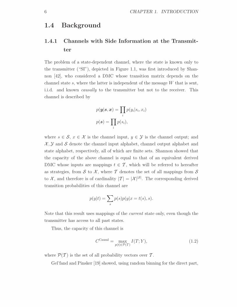
The problem of a state-dependent channel, where the state is known only to
the transmitter (“SI”), depicted in Figure 1.1, was first introduced by Shan-
non [42], who considered a DMC whose transition matrix depends on the
channel state s, where the latter is independent of the message W that is sent,
i.i.d. and known causally to the transmitter but not to the receiver. This
channel is described by
p(y|s,x) =∏
i
p(yi|si, xi)
p(s) =∏
i
p(si),
where s ∈ S, x ∈ X is the channel input, y ∈ Y is the channel output; and
X ,Y and S denote the channel input alphabet, channel output alphabet and
state alphabet, respectively, all of which are finite sets. Shannon showed that
the capacity of the above channel is equal to that of an equivalent derived
DMC whose inputs are mappings t ∈ T , which will be referred to hereafter
as strategies, from S to X , where T denotes the set of all mappings from Sto X , and therefore is of cardinality |T | = |X ||S|. The corresponding derived
transition probabilities of this channel are
p(y|t) =∑
s
p(s)p(y|x = t(s), s).
Note that this result uses mappings of the current state only, even though the
transmitter has access to all past states.
Thus, the capacity of this channel is
CCausal = maxp(t)∈P(T )
I(T ;Y ), (1.2)
where P(T ) is the set of all probability vectors over T .
Gel’fand and Pinsker [19] showed, using random binning for the direct part,
1.4. BACKGROUND 7
Channel
Encoder Decoder
S
p(y|x, s)Y WXW
Figure 1.1: The discrete memoryless channel with SI at the transmitter.
that the capacity of the above channel, when the state s is known non-causally
to the transmitter, is given by
Cnoncausal = maxp(u,x|s)
{I(U ;Y ) − I(U ;S)}, (1.3)
where the maximum is over all joint distributions of the form p(s)p(u, x|s)p(y|x, s),and U is an “auxiliary” random variable from a finite set, whose cardinality
need not exceed |U| ≤ |X | + |S|.Both of this results can be extended to continuous memoryless channels.
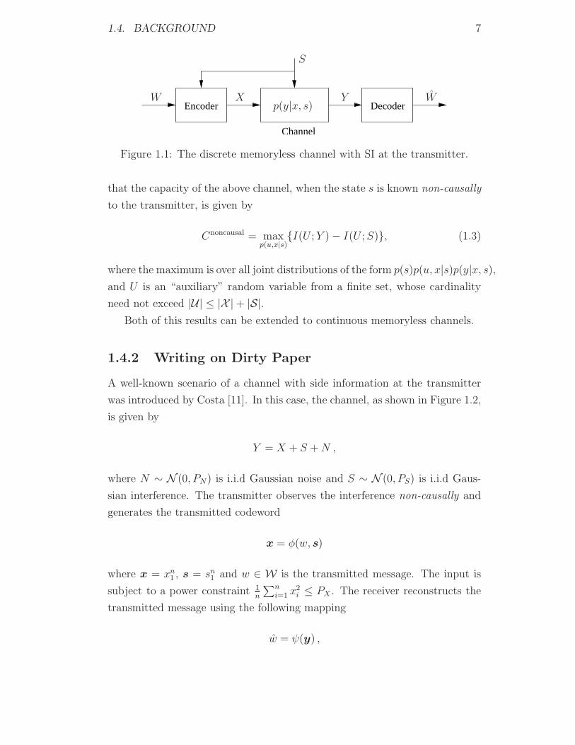
1.4.2 Writing on Dirty Paper
A well-known scenario of a channel with side information at the transmitter
was introduced by Costa [11]. In this case, the channel, as shown in Figure 1.2,
is given by
Y = X + S +N ,
where N ∼ N (0, PN) is i.i.d Gaussian noise and S ∼ N (0, PS) is i.i.d Gaus-
sian interference. The transmitter observes the interference non-causally and
generates the transmitted codeword
x = φ(w, s)
where x = xn1 , s = sn
1 and w ∈ W is the transmitted message. The input is
subject to a power constraint 1n
∑ni=1 x
2i ≤ PX . The receiver reconstructs the
transmitted message using the following mapping
w = ψ(y) ,
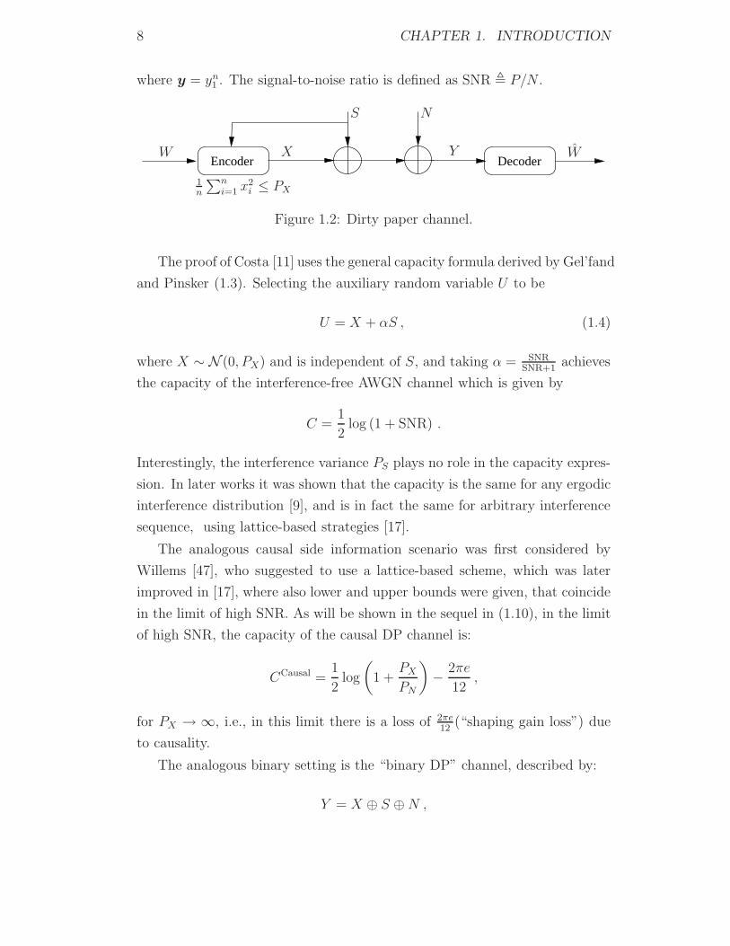
8 CHAPTER 1. INTRODUCTION
where y = yn1 . The signal-to-noise ratio is defined as SNR � P/N .
Encoder DecoderX
1n
∑ni=1 x
2i ≤ PX
W Y
S N
W
Figure 1.2: Dirty paper channel.
The proof of Costa [11] uses the general capacity formula derived by Gel’fand
and Pinsker (1.3). Selecting the auxiliary random variable U to be
U = X + αS , (1.4)
where X ∼ N (0, PX) and is independent of S, and taking α = SNRSNR+1
achieves
the capacity of the interference-free AWGN channel which is given by
C =1
2log (1 + SNR) .
Interestingly, the interference variance PS plays no role in the capacity expres-
sion. In later works it was shown that the capacity is the same for any ergodic
interference distribution [9], and is in fact the same for arbitrary interference
sequence, using lattice-based strategies [17].
The analogous causal side information scenario was first considered by
Willems [47], who suggested to use a lattice-based scheme, which was later
improved in [17], where also lower and upper bounds were given, that coincide
in the limit of high SNR. As will be shown in the sequel in (1.10), in the limit
of high SNR, the capacity of the causal DP channel is:
CCausal =1
2log
(1 +
PX
PN
)− 2πe
12,
for PX → ∞, i.e., in this limit there is a loss of 2πe12
(“shaping gain loss”) due
to causality.
The analogous binary setting is the “binary DP” channel, described by:
Y = X ⊕ S ⊕N ,

1.4. BACKGROUND 9
where X,S,N ∈ Z2 and ⊕ denotes addition mod 2 (XOR). The input con-
straint is 1nwH(x) ≤ q, where 0 ≤ q ≤ 1/2, wH(·) denotes Hamming weight,
and n is the length of the codeword. The noiseN ∼ Bernoulli(ε) is independent
of (S,X) (w.l.o.g. we assume ε ≤ 12) ; the state information (“interference”)
S ∼ Bernoulli (1/2) is known either causally or non-causally to the encoder.
The capacity of this binary DP channel with non-causal knowledge of the
interference is equal to (see [2, 53]):
Cnoncausaldirty = uch max {Hb(q) − Hb(ε), 0} , (1.5)
where Hb(·) denotes the binary entropy [12] and uch is the upper convex hull
operation with respect to q. Thus, unlike in the Gaussian setting, in the
binary case the capacity of the dirty channel is strictly lower than that of the
corresponding interference-free (“clean”) channel,
Cclean = Hb(q � ε) −Hb(ε) , (1.6)
due to the binary convolution (denoted by �) with ε in the first element, which
increases entropy, and is defined as:
q1 � q2 � (1 − q1)q2 + q1(1 − q2) .
The capacity of the causal binary DP channel can be easily derived from (1.2),
and is equal to:
Ccausaldirty = 2q (1 −Hb(ε)) ,
meaning that the best possible strategy, in the causal case, is to use all pos-
sible transmitting power to eliminate the interference S from as much input
symbols inside a block of size n as possible (2qn slots on average) and to send
information over the binary symmetric channel (BSC) with error probability
ε, that was obtained for these symbols.

10 CHAPTER 1. INTRODUCTION
1.4.3 Lattice-Strategies
Preliminary: Lattices
An n-dimensional lattice Λ is a discrete group in the Euclidian space Rn which
is closed with respect to the addition operation (over R) [10]. The lattice is
specified by
Λ = {λ = Gi : i ∈ Zn},
where G is an n × n real valued matrix, called the generator matrix of the
lattice (whose choice is not unique). A coset of the lattice is any translation
of the original lattice Λ, i.e., a + Λ where a ∈ Rn.
The nearest neighbor quantizer QΛ(·) associated with Λ is defined by
QΛ(x) = λ ∈ Λ if ||x − λ|| ≤ ||x − λ′||, ∀ λ′ ∈ Λ,
where || · || denotes Euclidian norm. The Voronoi region associated with a
lattice point λ is the set of all points in Rn that are closer (in Euclidian
distance) to λ than to any other lattice point. Specifically, the fundamental
Voronoi region is defined as the set of all points that are closest to the origin
V0 � {x ∈ Rn : QΛ(x) = 0},
where ties are broken arbitrarily. The modulo lattice operation with respect
to Λ is defined as
x mod Λ = x −QΛ(x).
This operation satisfies the following distributive property
[x mod Λ + y] mod Λ = [x + y] mod Λ.
The second moment of a lattice Λ is given by
σ2Λ �
1n
∫V0||x||2dx
V,

1.4. BACKGROUND 11
where V is the volume of the fundamental Voronoi region, i.e., V =∫V0
dx (the
same for all Voronoi regions of Λ). The normalized second moment is given by
G(Λ) � σ2Λ
V 2/n.
The normalized second moment is always greater than 1/2πe (see [52]). It is
known [52] that for sufficiently large dimension there exist lattices that are
good for quantization (these lattices are also known to be good for shaping
[16]), in the sense that for any ε > 0
log(2πeG(Λ)) < ε, (1.7)
for large enough n. In addition, there exist lattices with second moment P
that are good for AWGN channel coding [16], satisfying
Pr(X �∈ V0) < ε, where X ∼ N (0, (P − ε)In), ∀ε > 0,
where In is an n× n identity matrix.
The differential entropy of an n-dimensional random vector U , which is
distributed uniformly over the fundamental Voronoi cell, i.e., U ∼ Unif(V0),
is given by [52]
h(U) = log(V )
= log
(σ2
Λ
G(Λ)
)n/2
=n
2log
(σ2
Λ
G(Λ)
)
≈ n
2log
(2πeσ2
Λ
),
where the last (approximate) equality holds for lattices that are good for quan-
tization, for large n. For one-dimensional lattices, i.e., cZ, the differential
entropy of U is equal to
h(U) = log(12σ2Λ).

12 CHAPTER 1. INTRODUCTION
Lattice-Strategies for Cancelling Known Interference
The capacity of the dirty-paper channel (1.1) can also be achieved using a
coding scheme based on lattice-strategies (also known as lattice precoding) [17,
53]. Specifically, let Λ be an n-dimensional lattice with second moment PX that
is good for quantization (1.7). The information bearing signal V is distributed
uniformly over the basic cell of Λ, i.e., V ∼ Unif(V0). The transmission scheme
is shown in Figure 1.3.
−
−
Channel DecoderEncoder
U
αV
N
S
αS
+ ++ mod-Λ YX mod-Λ Y ′
Figure 1.3: Lattice-strategies transmission scheme.
• Transmitter : The transmitter output is the error vector between V and
αS + U , i.e.,
X =[V − αS − U
]mod Λ,
where U ∼ Unif(V0) is common randomness (“dither”) which is known
to both, the transmitter and the receiver. From the dither property [52],
X ∼ Unif(V0) (and is independent of V ), and hence the power constraint
is satisfied.
• Receiver : The channel output Y is multiplied by α, followed by the
dither addition modulo-Λ, i.e.,
Y ′ = [αY + U ] mod Λ.
Erez, Shamai and Zamir showed in [17] that the equivalent channel is an
interference-free modulo-Λ channel, i.e.,
Y ′ =[V + N eff
]mod Λ, (1.8)

1.4. BACKGROUND 13
where Neff is the effective noise which is given by
N eff = −(1 − α)X + αN , (1.9)
and is independent of V since X is independent of V due to the dither and
(X,V ) are independent of N . Moreover, X and U have the same distribution,
and hence the effective noise of (1.9) is equivalent, in distribution, to
N eff = (1 − α)U + αN .
For α = 1, the interference concentration is reflected in the above modulo-Λ
equivalent channel (1.8) and (1.9). That is, the residual interference at the de-
coder is concentrated on discrete values (due to the modulo operation), which
are the lattice points of Λ. Nevertheless, this is not the optimal selection of α.
A better selection is the one that minimize the power of Neff, i.e., α = SNRSNR+1
(which is exactly the choice of α in the Costa scheme), which allows to achieve
all rates satisfying:
R ≤ 1
2log (1 + SNR) − 1
2log (2πeG(Λ)) . (1.10)
Taking a sequence of lattices Λ, with increasing dimension, that are good
for quantization (1.7) (G(Λ) → 12πe
), it follows that one can achieve rates ap-
proaching 12log (1 + SNR), i.e., the capacity of an interference-free AWGN
channel [17, 53]. Nevertheless this is possible only when the interference is
known non-causally. In case, the interference is known only causally, one
cannot anticipate the interference of future symbols, and is limited to one-
dimensional (“scalar”) lattice strategies. For this channels only rates satisfying
R ≤ 1
2log (1 + SNR) − 1
2log
(2πe
12
),
can be achieved, using this strategy, as G(Λ) = 1/12 for such lattices. Note
that the one-dimensional lattice scheme can be seen as an extension of the
intersymbol interference (ISI) cancellation scheme suggested independently by
Tomlinson [45] and Harashima [22]. Hence, we shall refer to this scheme and
its extensions as Tomlinson-Harashima precoding (THP).

14 CHAPTER 1. INTRODUCTION
1.4.4 Compound Channels
Encoder Decoder
Channel
Y WXWpβ(y|x, s)
β ∈ B
Figure 1.4: The discrete compound memoryless channel.
A discrete memoryless compound channel is a channel whose transition
matrix depends on a parameter β, which is constant and not known to the
transmitter but is known to the receiver3 and takes values from B, where the
alphabet B is a finite set. See Figure 1.4.
The (“worst-case”) capacity of this channel was found, by several different
authors [4, 14, 48] (see also [49]), to be
C = maxp(x)∈P(X)
infβ∈B
Iβ(X;Y ),
where Iβ(X;Y ) denotes the mutual information of X and Y with respect to
the transition matrix pβ(y|x) and P(X ) is the set of all probability vectors
over X .
This result can be extended to continuous memoryless channels, as well.
1.4.5 Compound Channels With SI at the Transmitter
The generalization of the two problems of Chapter 1.4.1 and Chapter 1.4.4 is
that of a discrete-memoryless compound state-dependent channel, where the
state is available (as SI) at the transmitter, depicted in Figure 1.5.
This problem was treated, for the non-causal case, by Mitran, Devroye and
Tarokh in [33], where they extended the proof of Gel’fand and Pinsker [19]
to the compound case, but due to the presence of the channel outputs Y i1 in
the auxiliary variable U in the converse part, their achievable rate and upper
bound do not coincide in general, and thus they were only able to derive inner
3Sometimes a channel is said to be compound if β is not known at both ends. Thecapacity however is the same in both scenarios (see, e.g., [49, chap. 4]), as the receiver mayestimate β to within any desired accuracy (with probability going to one), using a negligibleportion of the block length.

1.4. BACKGROUND 15
Channel
Encoder Decoder
S
Y WXWpβ(y|x, s)
Figure 1.5: The compound discrete memoryless channel with SI at the trans-mitter.
and outer bounds on the capacity:
Cl ≤ C ≤ Cu
Cl = supp(u|x,s,w)p(x|s,w)p(w)
infβ∈B
[Iβ(U ;Y |W ) − I(U ;S|W )]
Cu = suppβ(u|x,s,w)p(x|s,w)p(w)
infβ∈B
[Iβ(U ;Y |W ) − I(U ;S|W )] ,
where the suprema are over all finite alphabet auxiliary random variables U and
finite alphabet time-sharing random variables W , and {pβ(u|x, s, w)} denotes
any family of distributions, where a distribution p(u|x, s, w) is chosen for each
value of β before the infimum over β is computed.
The authors of [33] extended these bounds to continuous alphabets and
considered the following compound version of the DP channel:
Y = β1X + β2S +N , (1.11)
where the interference sequence S is known non-causally and the compound
channel parameter is β = (β1, β2). They suggest using the same auxiliary
variable that was used by Costa for the non-compound case (given in (1.4))
and derive lower and upper bounds on the performance for this choice.
1.4.6 Gaussian MIMO Broadcast Channels
The generalK-user real-valued 4 multiple-input multiple-output (MIMO) chan-
nel with M antennas at the transmitter and N antennas at each receiver, is
4The complex case is defined in a similar manner. See, e.g., [6, 51].

16 CHAPTER 1. INTRODUCTION
defined by
Y k = HkX + N k, k = 1, ..., K ,
where Hk ∈ RN×M is the channel gain matrix of user k, X is the transmit
signal vector, subject to some power constraint (depending on the scenario of
interest and N k is a Gaussian noise vector, which w.l.o.g. has zero-mean and
identity covariance matrix Ik.5
Different scenarios for this channel were considered. We shall focus our
interest on the private-message scenario, in which a different (“private”) mes-
sage needs to be conveyed to each of the users (in contrast to the common
message scenario, in which the same message is transmitted to all users), and
the power allocated to each of the messages is Pi.
For this scenario, different transmission schemes were proposed, the two
most prominent being the linear transmission schemes and the ones that use
DPC (see, e.g., [6]).
To further simplify the setting and give a geometrical view of this problem,
we shall consider only the 2-user case with Kt = 2 transmit antennas and
Kr = 1 receive antenna at each receiver:
Yi = hTi X +Ni, i = 1, 2 (1.12)
where X and hi are 2 × 1 vectors.
Hence, for linear zero-forcing (ZF) or linear MMSE, as well as for DPC
based schemes, the transmitted signal can be decomposed into a sum of the
two message signals, meant for both users:
x = x1 + x2,
xi = xiti
where xi is the scalar information signal (can take, both, positive and negative
values) intended for user i of average power Pi, and ti is a unit vector in the
direction of the transmitted direction of this information signal. Without loss
of generality, we shall assume that P2 ≥ P1, and define SNRi = Pi (i = 1, 2).
5Otherwise the receiver can subtract the noise mean vector from the channel output andmultiply the result by a whitening-matrix.
1.4. BACKGROUND 17
θ
h1
h2
x1
x2
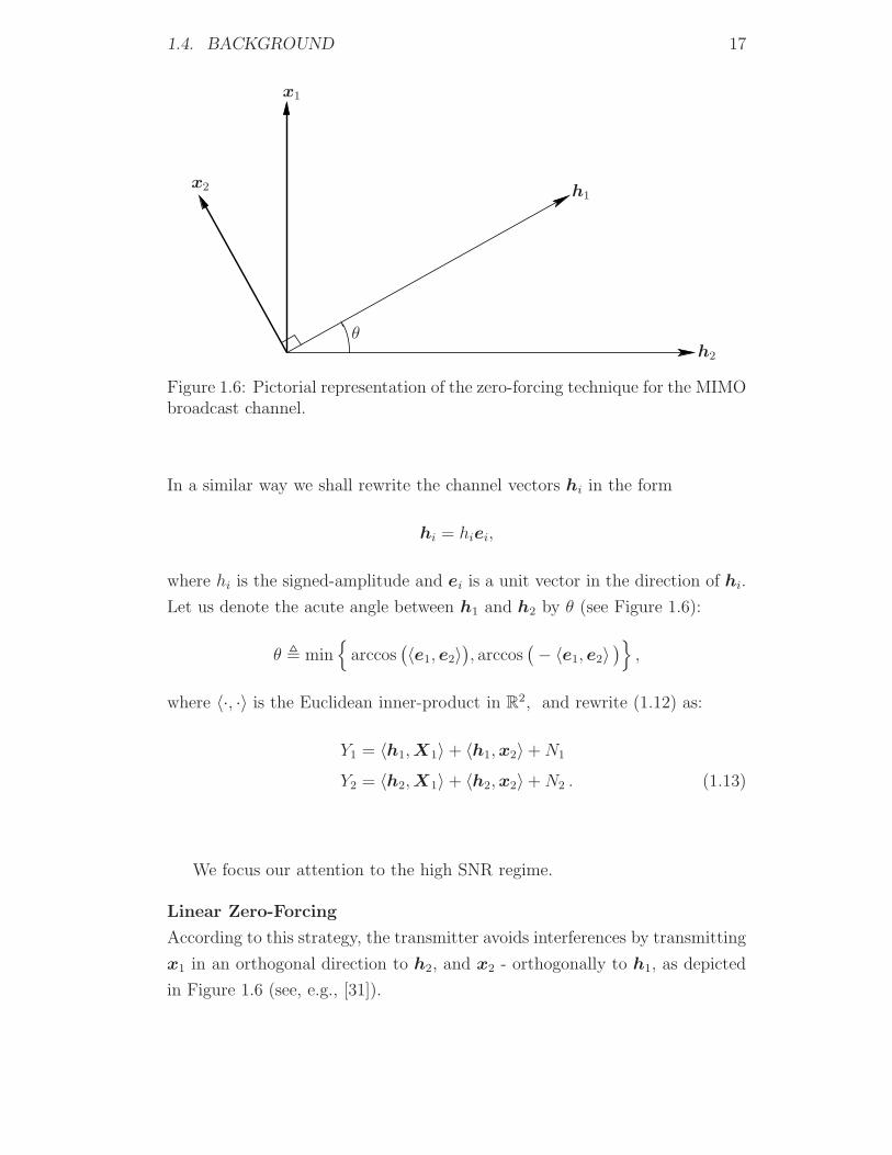
Figure 1.6: Pictorial representation of the zero-forcing technique for the MIMObroadcast channel.
In a similar way we shall rewrite the channel vectors hi in the form
hi = hiei,
where hi is the signed-amplitude and ei is a unit vector in the direction of hi.
Let us denote the acute angle between h1 and h2 by θ (see Figure 1.6):
θ � min{
arccos(〈e1, e2〉
), arccos
(− 〈e1, e2〉
)},
where 〈·, ·〉 is the Euclidean inner-product in R2, and rewrite (1.12) as:
Y1 = 〈h1,X1〉 + 〈h1,x2〉 +N1
Y2 = 〈h2,X1〉 + 〈h2,x2〉 +N2 . (1.13)
We focus our attention to the high SNR regime.
Linear Zero-Forcing
According to this strategy, the transmitter avoids interferences by transmitting
x1 in an orthogonal direction to h2, and x2 - orthogonally to h1, as depicted
in Figure 1.6 (see, e.g., [31]).

18 CHAPTER 1. INTRODUCTION
Hence, we may rewrite the channel outputs (1.13) as:6
Yi = 〈hi,X i〉 +Ni
= Xihi cos(π
2− θ
)+Ni
= Xihi sin(θ) +Ni, i = 1, 2.
Note that this approach provides, effectively, two parallel channels. Finally,
using codebooks generated in an i.i.d. Gaussian manner (with mean 0 and
variance Pi), the following rates are achieved:
Ri = I(Xi ;Yi) =1
2log
(1 + SNRih
2i sin2(θ)
)i = 1, 2 . (1.14)
Zero-Forcing Dirty Paper Coding
Instead of using linear precoding approaches, one may transmit the message
to user 1 in an orthogonal direction to the channel vector of user 2, and apply
dirty paper coding to eliminate the interference of user 2 on its own channel
vector. This way, user 2 is free of interferences from the signal of user 1
and can transmit its information signal in the best possible direction, i.e., e2
(see Figure 1.7), and by this outperform the rates achievable via linear schemes.
The expressions we provide below are for the non-causal case, i.e., correspond
to using multi-dimensional THP where the dimension goes to infinity.7
Without loss of generality, we take the user that performs DPC to be user
1, i.e., 〈h2, x1〉 = 0. Thus,
Y2 = 〈h2, X2〉 +N2
= h2X2 +N2
Y1 = 〈h1, X1〉 + 〈h1, x2〉 +N1 ,
= h1X1 sin(θ) + h1X2 cos(θ) +N1 . (1.15)
6 This is true up to a possible additional phase of p inside the cosine, which has no effecton the effective channel, since the receiver knows the channel
7The results for the causal case are identical up to a subtraction of the shaping loss12 log
(2πe12
).

1.4. BACKGROUND 19
θ
h1
h2
x1
x2
Figure 1.7: Pictorial representation of the ZF-DPC technique in the MIMObroadcast channel.
Dividing both sides of (1.15) by h1 sin(θ) gives rise to the equivalent channel
Y1 = X1 +X2ctg(θ) +1
h1 sin(θ)N1 .
Now, by using the dirty paper coding scheme of Chapter 1.4.3, user 1 can
effectively eliminate the interference of user 2:
X1 = [v1 − α · ctg(θ)X2 − U ] mod Λ
Y ′1 = [αY1 + U ] mod Λ
=
[v1 − (1 − α)X1 +
α
h1 sin(θ)N2
]mod Λ , (1.16)
where U is a dither distributed uniformly over the basic Voronoi cell V0 of
the lattice Λ, whose second moment is set to be P1. Finally, by setting the
distributions of V1 and X2 to be uniform over V0 and Gaussian with power P2,
respectively, we obtain the following rates:
R1 =1
2log
(1 + SNR1h
21 sin2(θ)
),
R2 =1
2log
(1 + SNR2h
22
).
Note that indeed, the rate of user 1 is the same as in (1.14), but the rate of
20 CHAPTER 1. INTRODUCTION
user 2 has improved over the that of the linear ZF scheme.
Remark 1.1. Both the linear ZF and the ZF-DPC schemes can be improved
by taking into account the noise power, rather than totaly eliminate the cross-
interferences from the other user (see linear MMSE and MMSE-DPC in [6]).
Nevertheless, when the SNRs are high the performance of the MMSE schemes
coincide with those of the ZF ones.
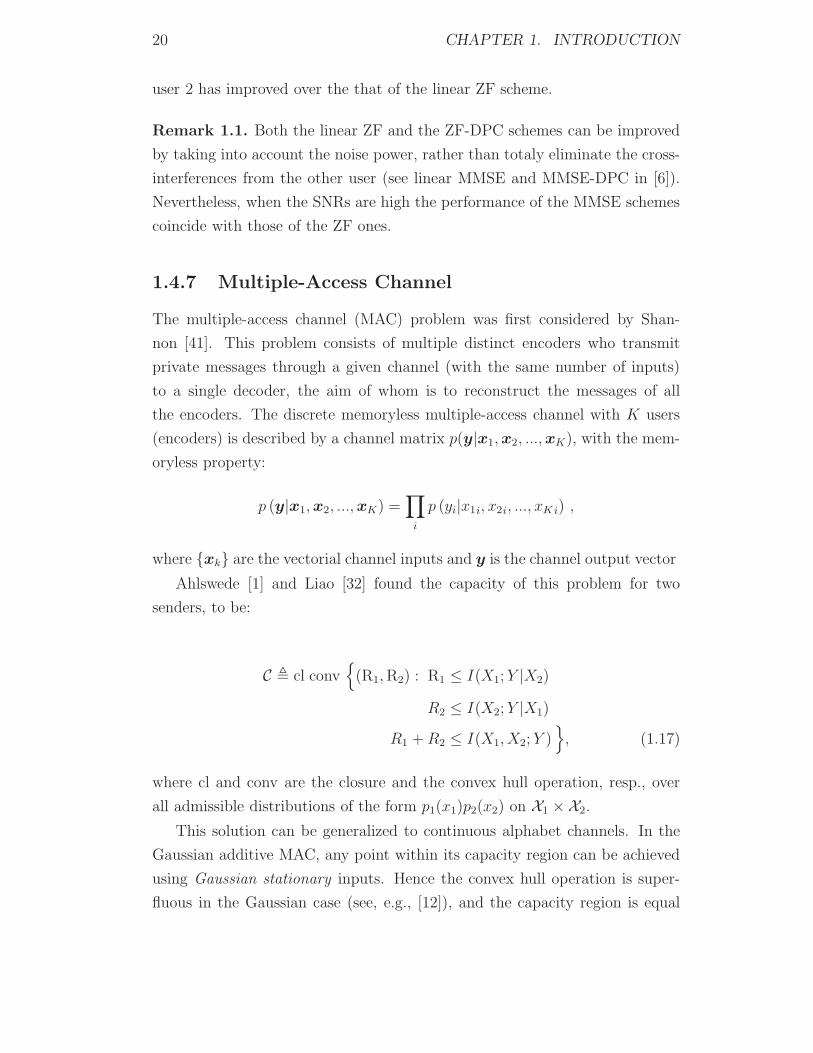
1.4.7 Multiple-Access Channel
The multiple-access channel (MAC) problem was first considered by Shan-
non [41]. This problem consists of multiple distinct encoders who transmit
private messages through a given channel (with the same number of inputs)
to a single decoder, the aim of whom is to reconstruct the messages of all
the encoders. The discrete memoryless multiple-access channel with K users
(encoders) is described by a channel matrix p(y|x1,x2, ...,xK), with the mem-
oryless property:
p (y|x1,x2, ...,xK) =∏
i
p (yi|x1i, x2i, ..., xKi) ,
where {xk} are the vectorial channel inputs and y is the channel output vector
Ahlswede [1] and Liao [32] found the capacity of this problem for two
senders, to be:
C � cl conv{
(R1,R2) : R1 ≤ I(X1;Y |X2)
R2 ≤ I(X2;Y |X1)
R1 +R2 ≤ I(X1, X2;Y )}, (1.17)
where cl and conv are the closure and the convex hull operation, resp., over
all admissible distributions of the form p1(x1)p2(x2) on X1 ×X2.
This solution can be generalized to continuous alphabet channels. In the
Gaussian additive MAC, any point within its capacity region can be achieved
using Gaussian stationary inputs. Hence the convex hull operation is super-
fluous in the Gaussian case (see, e.g., [12]), and the capacity region is equal

1.4. BACKGROUND 21
to:
C �{
(R1, R2) : R1 ≤1
2log(1 + SNR1)
R2 ≤1
2log(1 + SNR2)
R1 +R2 ≤1
2log(1 + SNR1 + SNR2)
},
where SNR1 and SNR2 are the signal-to-noise ratios of users 1 and 2, respec-
tively.
1.4.8 Dirty Multiple-Access Channel
Consider the two-user memoryless state-dependent multiple-access channel
(MAC) with transition and state probability distributions
p(y|x1, x2, s) and p(s) ,
where s ∈ S or parts of it are known causally or non-causally at one or both
encoders. The channel inputs are x1 ∈ X1 and x2 ∈ X2, and the channel output
is y ∈ Y . The memoryless property of the channel implies that
p(y|x1,x2, s) =n∏
i=1
p(yi|x1i, x2i, si).
Its capacity region is still not known in general, for the different SI scenarios,
and remains an open problem. See, e.g., [36].
This model can be seen as a generalization of the point-to-point with SI at
the transmitter, described in Chapter 1.4.1. Trying to generalize the random
binning scheme of Gel’fand and Pinsker provides the achievable region (see,
e.g., [36]):
R � cl conv{
(R1,R2) : R1 ≤ I(U ;Y |V ) − I(U ;S|V )
R2 ≤ I(V ;Y |U) − I(V ;S|U)
R1+R2 ≤ I(U, V ;Y ) − I(U, V ;S)}

22 CHAPTER 1. INTRODUCTION
Enc. 1
Enc. 2
Dec
X1
X2
W1
W2
Y W1
W2
S
N
Figure 1.8: Dirty MAC with common state information.
where (U, V ) are auxiliary pairs satisfying:
(U,X1) ↔ S ↔ (V,X2)
(U, V ) ↔ (X1, X2, S) ↔ Y.
However, this scheme was proved to be suboptimal by Philosof and Zamir [35],
at least in certain cases, when the users have access to two distinct independent
parts of the state s.
Philosof et al. [34, 38, 35] considered a Gaussian additive MAC with ad-
ditive interference and composed of a sum of two independent Gaussian in-
terferences, where each interference is known non-causally only to one of the
encoders. They called this channel the “doubly-dirty MAC”. The capacity
region of the Gaussian “dirty MAC”, where the interference is known non-
causally to both transmitters (“DMAC with common interference”), was found
by Gel’fand and Pinsker [20] (and rediscovered by Kim, Sutivong and Sig-
urjonsson [27]), to be equal to the interference-free MAC channel, by applying
DPC by both users.
Philosof, Zamir and Erez [37] considered a binary modulo-additive version
of this channel (“binary DMAC”), depicted also in Figure 1.8:
Y = X1 ⊕X2 ⊕ S ⊕N , (1.18)
where X1, X2, S,N ∈ Z2. The input (“power”) constraints are 1nwH(xi) ≤ qi
for i = 1, 2, where 0 ≤ q1, q2 ≤ 1/2. The noise N ∼ Bernoulli(ε) and is
independent of S,X1, X2; the state information S ∼ Bernoulli (1/2) is known

1.4. BACKGROUND 23
non-causally to both encoders.
They derived the capacities for two different scenarios:
• The binary doubly-dirty MAC : in this scenario S = S1 ⊕ S2, where
S1, S2 ∼ Bernoulli(1/2) are independent and known non-causally to en-
coders 1 and 2, respectively. The capacity region of this channel is given
by the set of all rate pairs (R1, R2) satisfying:
C(q1, q2) �{
(R1, R2) : R1 +R2 ≤ uch [Hb(qmin) −Hb(ε)]},
where qmin � min(q1, q2) and the upper convex hull operation is w.r.t.
q1 and q2.
• The single informed user : in this scenario S is known only to user 1.
The capacity region of this channel is given by the set of all rate pairs
(R1, R2) satisfying:
C(q1, q2) � cl conv
{(R1, R2) :
R2 ≤ Hb(q2 � ε) −Hb(ε)
R1 +R2 ≤ Hb(q1) −Hb(ε)
}. (1.19)
However, contrary to the Gaussian case, in which the common interference
capacity region is the same as the interference-free region, and is achieved
using stationary inputs, in the binary DP channel, there is a loss even in the
point-to-point setting. Thus the capacity region of the binary DMAC with
common interference is not known, and is yet to be determined.

Chapter 2
Robustness of Dirty Paper
Coding
In this chapter we consider a Gaussian DP channel, where the trans-
mitter knows the interference sequence up to a constant multiplica-
tive factor, known only to the receiver. we derive lower bounds on
the achievable rate of communication by proposing a lattice-based
coding scheme that partially compensates for the imprecise channel
knowledge. We focus on a communication scenario where the SNR
is high. When the power of the interference is finite, we show that
the achievable rate of this coding scheme may be improved by a ju-
dicious choice of the scaling parameter at the receiver. We further
show that the communication rate may be improved, for finite as
well as infinite interference power, by allowing randomized scaling
at the transmitter of the lattice-based scheme, as well as in Costa’s
random binning scheme. Finally we consider the implications of the
results on the Gaussian MIMO BC channel with imprecise channel
knowledge. We employ the derived technique on the DPC and linear
transmission schemes, and compare their performance.
24
2.1. CHANNEL MODEL AND MOTIVATION 25
Encoder DecoderX
1n
∑ni=1 x
2i ≤ PX
S
1β
W
N
Y W
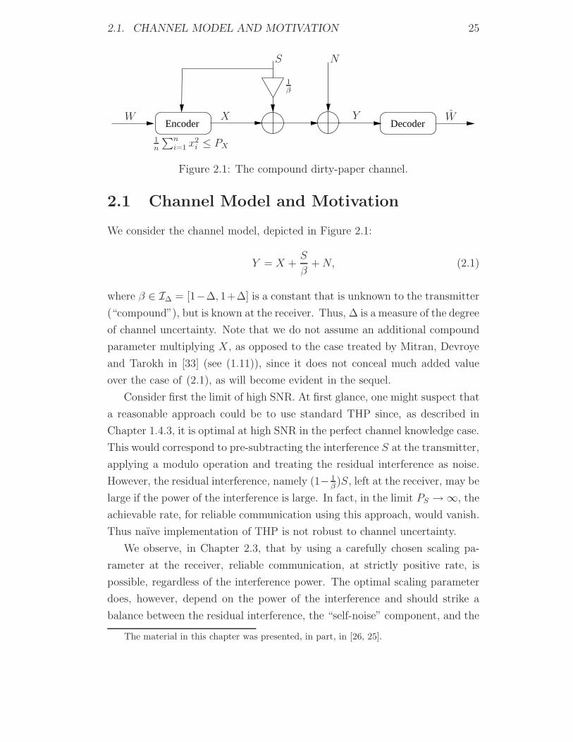
Figure 2.1: The compound dirty-paper channel.
2.1 Channel Model and Motivation
We consider the channel model, depicted in Figure 2.1:
Y = X +S
β+N, (2.1)
where β ∈ IΔ = [1−Δ, 1+Δ] is a constant that is unknown to the transmitter
(“compound”), but is known at the receiver. Thus, Δ is a measure of the degree
of channel uncertainty. Note that we do not assume an additional compound
parameter multiplying X, as opposed to the case treated by Mitran, Devroye
and Tarokh in [33] (see (1.11)), since it does not conceal much added value
over the case of (2.1), as will become evident in the sequel.
Consider first the limit of high SNR. At first glance, one might suspect that
a reasonable approach could be to use standard THP since, as described in
Chapter 1.4.3, it is optimal at high SNR in the perfect channel knowledge case.
This would correspond to pre-subtracting the interference S at the transmitter,
applying a modulo operation and treating the residual interference as noise.
However, the residual interference, namely (1− 1β)S, left at the receiver, may be
large if the power of the interference is large. In fact, in the limit PS → ∞, the
achievable rate, for reliable communication using this approach, would vanish.
Thus naıve implementation of THP is not robust to channel uncertainty.
We observe, in Chapter 2.3, that by using a carefully chosen scaling pa-
rameter at the receiver, reliable communication, at strictly positive rate, is
possible, regardless of the interference power. The optimal scaling parameter
does, however, depend on the power of the interference and should strike a
balance between the residual interference, the “self-noise” component, and the
The material in this chapter was presented, in part, in [26, 25].

26 CHAPTER 2. ROBUSTNESS OF DIRTY PAPER CODING
Gaussian noise.
We then show, in Chapter 2.4, that performance may further be improved
by using randomized (time-varying) scaling at the transmitter. We begin by
examining the more general problem of compound channel with side informa-
tion, introduced in Chapter 1.4.5.
2.2 Compound Channels with Causal Side In-
formation at the Transmitter
The compound DP channel of (2.1) is a compound memoryless state-dependent
channel with SI at the transmitter, as argued in Chapter 1.4.5, where S is the
SI and β plays the role of the compound component (IΔ plays the role of B).
The (worst-case) capacity formula for the (“classical”) compound channel,
derived by Shannon [42], may be easily extended to the case of a compound
channel with SI available causally to the transmitter, as implied by the follow-
ing theorem, which is proved in Appendix A.1.
Theorem 2.1. The worst-case capacity of a compound DMC with causal SI
at the transmitter is given by
C = maxp(t)∈P(T )
infβ∈B
Iβ(T ;Y ) ,
where T denotes the set of all strategy functions of the form t : S −→ X , and
P(T ) is the set of all probability vectors over T .
Remark 2.1.
• The result of Theorem 2.1 suggest that, like in the non-compound DMC
with causal SI problem (see Chapter 1.4.1), only mappings of the current
state needs to be considered.
• The case of non-causal SI is more difficult. The converse of Gel’fand-
Pinsker [19] is not easily extended to the compound scenario, as briefly
discussed in Chapter 1.4.5, and only upper and lower single-letter bounds
on the capacity with non-causal SI, are known. Using Theorem 2.1, a
non single-letter expression for the worst-case capacity in the non-causal

2.3. COMPENSATION FOR CHANNEL UNCERTAINTY AT TX 27
SI case, using k-dimensional vector strategies and taking k to infinity,
follows:
Cnon−casual = lim supk→∞
maxp(t)
infβ
1
kIβ(T ; Y ) .
2.3 Compensation for Channel Uncertainty at
the Transmitter
The compound DP channel was defined in (2.1). In this section, we consider
the case of i.i.d. interference of finite power PS. The results of Chapter 2.2
may readily be extended to continuous alphabet and to incorporate an input
constraint (similarly to [33], Sec. IV). Thus, Theorem 2.1 holds for this setting
as well.
Since the capacity of the dirty-paper channel with causal SI is unknown
even in the standard (non compound) setting, we do not attempt to explicitly
find the capacity in the compound setting. Rather, we shall examine the
performance of THP-like precoding schemes and suggest methods by which
the lack of perfect channel knowledge at the transmitter may be taken into
account and partially compensated for.
2.3.1 THP With Imprecise Channel Knowledge
We shall concentrate on the performance of one-dimensional lattice based
schemes, i.e., lattices of the form Λ = LZ, whose fundamental Voronoi re-
gion is V0 �[−L
2L2
), where L is chosen such that the power constraint is
satisfied: PX = L2
12. Denote by SIR � β2 PX
PSthe signal-to-interference ratio.
Let U ∼ Unif(V0) be a random variable (dither) known to both transmitter
and receiver. We consider a variation of the THP scheme of Chapter 1.4.3, in
which we distinguish between the inflation factors “α”, used at the transmitter
and the receiver:
• Transmitter: for any v ∈ V0, the transmitted signal is
X = [v − αTS − U ] mod Λ.
28 CHAPTER 2. ROBUSTNESS OF DIRTY PAPER CODING
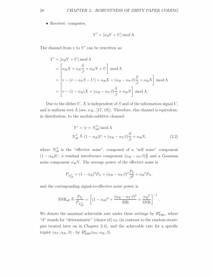
• Receiver: computes,
Y ′ = [αRY + U ] mod Λ.
The channel from v to Y ′ can be rewritten as:
Y ′ = [αRY + U ] mod Λ
=
[αRX + αR
S
β+ αRN + U
]mod Λ
=
[v − (v − αTS − U) + αRX + (αR − αTβ)
S
β+ αRN
]mod Λ
=
[v − (1 − αR)X + (αR − αTβ)
S
β+ αRN
]mod Λ .
Due to the dither U , X is independent of S and of the information signal V ,
and is uniform over Λ (see, e.g., [17, 18]). Therefore, this channel is equivalent,
in distribution, to the modulo-additive channel:
Y ′ = [v +Nβeff] mod Λ
Nβeff � (1 − αR)U + (αR − αTβ)
S
β+ αRN, (2.2)
where Nβeff is the “effective noise”, composed of a “self noise” component
(1 − αR)U , a residual interference component (αR − αTβ)Sβ
and a Gaussian
noise component αRN . The average power of the effective noise is
PNβeff
= (1 − αR)2PX + (αR − αTβ)2PS
β2+ αR
2PN .
and the corresponding signal-to-effective noise power is
SNReff � PX
PNβeff
=
[(1 − αR)2 +
(αR − αTβ)2
SIR+
αR2
SNR
]−1
.
We denote the maximal achievable rate under these settings by RdTHP, where
“d” stands for “deterministic” (choice of) αT (in contrast to the random strate-
gies treated later on in Chapter 2.4), and the achievable rate for a specific
triplet (αT , αR, β) - by RdTHP(αT , αR, β).
2.3. COMPENSATION FOR CHANNEL UNCERTAINTY AT TX 29
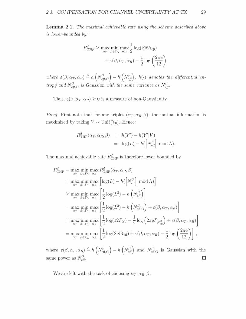
Lemma 2.1. The maximal achievable rate using the scheme described above
is lower-bounded by:
RdTHP ≥ max
αT
minβ∈IΔ
maxαR
1
2log(SNReff)
+ ε(β, αT , αR) − 1
2log
(2πe
12
),
where ε(β, αT , αR) � h(Nβ
eff,G
)− h
(Nβ
eff
), h(·) denotes the differential en-
tropy and Nβeff,G is Gaussian with the same variance as Nβ
eff.
Thus, ε(β, αT , αR) ≥ 0 is a measure of non-Gaussianity.
Proof. First note that for any triplet (αT , αR, β), the mutual information is
maximized by taking V ∼ Unif(V0). Hence:
RdTHP(αT , αR, β) = h(Y ′) − h(Y ′|V )
= log(L) − h([Nβ
eff
]mod Λ).
The maximal achievable rate RdTHP is therefore lower bounded by
RdTHP = max
αT
minβ∈IΔ
maxαR
RdTHP(αT , αR, β)
= maxαT
minβ∈IΔ
maxαR
[log(L) − h(
[Nβ
eff
]mod Λ)
]
≥ maxαT
minβ∈IΔ
maxαR
[1
2log(L2) − h
(Nβ
eff
)]
= maxαT
minβ∈IΔ
maxαR
[1
2log(L2) − h
(Nβ
eff,G
)+ ε(β, αT , αR)
]
= maxαT
minβ∈IΔ
maxαR
[1
2log(12PX) − 1
2log
(2πePNβ
eff
)+ ε(β, αT , αR)
]
= maxαT
minβ∈IΔ
maxαR
[1
2log(SNReff) + ε(β, αT , αR) − 1
2log
(2πe
12
)],
where ε(β, αT , αR) � h(Nβ
eff,G
)− h
(Nβ
eff
)and Nβ
eff,G is Gaussian with the
same power as Nβeff.
We are left with the task of choosing αT , αR, β.

30 CHAPTER 2. ROBUSTNESS OF DIRTY PAPER CODING
2.3.2 Naıve Approach
One could ignore the presence of the inaccuracy factor β and apply standard
THP, using the parameters αR = αT = αMMSE � SNR1+SNR
, which is the best selec-
tion of αR and αT in the perfect knowledge case, as discussed in Chapter 1.4.3.
This gives rise to the following signal-to-effective noise ratio at the receiver:
SNReff = λNaıve(β)(1 + SNR)
λNaıve(β) � 1
1 + 1SIR
+ SNRSIR
(1 − β)2.
Note that since (1 + SNR) is the output SNR in the perfect SI case, the
loss due to the imprecision (1 − β) is manifested in the multiplicative factor
0 < λNaıve(β) ≤ 1.
Moreover, when the interference is very strong, i.e., SIR → 0, even if the
SNR is high, the effective SNR goes to zero along with the rate (as further ex-
plained in Chapter 2.4.1). Nonetheless, a strictly positive rate can be achieved
in this scheme, using a smarter Rx-Tx pair, as is shown in the following sec-
tions.
2.3.3 Smart Receiver - Ignorant Transmitter
Using the fact that ε(β, αT , αR) ≥ 0, we can further loosen the lower-bound of
Lemma 2.1 to
RdTHP ≥ max
αT
minβ∈IΔ
maxαR
1
2log(SNReff) −
1
2log
(2πe
12
). (2.3)
Note that optimizing the r.h.s. of (2.3) is equivalent to maximizing SNReff
with respect to {αT , αR}. In this section we shall optimize with respect to αR
(“smart receiver”) and use αT = αMMSE � SNR1+SNR
(“ignorant transmitter”) as
was done in Chapter 2.3.2, and leave the treatment of a smarter selection of
αT (“smart transmitter”) to Chapter 2.4.
By solving the problem of maximizing the signal-to-effective noise ratio,
the following αR value and corresponding SNReff are obtained:
αMMSET = αMMSE � SNR
1 + SNR
2.3. COMPENSATION FOR CHANNEL UNCERTAINTY AT TX 31
0 5 10 15 20 25 30−10
−5
0
5
10
15
20
SNR [dB]
SN
Ref
f [dB
]
−10dB, MMSE−10dB, Naive0dB, MMSE0dB, Naive10dB, MMSE10dB, Naive
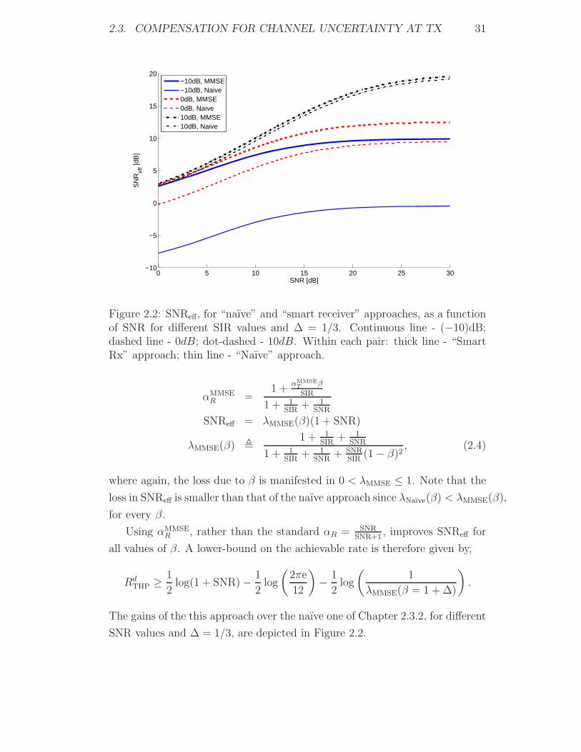
Figure 2.2: SNReff, for “naıve” and “smart receiver” approaches, as a functionof SNR for different SIR values and Δ = 1/3. Continuous line - (−10)dB;dashed line - 0dB; dot-dashed - 10dB. Within each pair: thick line - “SmartRx” approach; thin line - “Naıve” approach.
αMMSER =
1 +αMMSE
T β
SIR
1 + 1SIR
+ 1SNR
SNReff = λMMSE(β)(1 + SNR)
λMMSE(β) � 1 + 1SIR
+ 1SNR
1 + 1SIR
+ 1SNR
+ SNRSIR
(1 − β)2, (2.4)
where again, the loss due to β is manifested in 0 < λMMSE ≤ 1. Note that the
loss in SNReff is smaller than that of the naıve approach since λNaıve(β) < λMMSE(β),
for every β.
Using αMMSER , rather than the standard αR = SNR
SNR+1, improves SNReff for
all values of β. A lower-bound on the achievable rate is therefore given by,
RdTHP ≥ 1
2log(1 + SNR) − 1
2log
(2πe
12
)− 1
2log
(1
λMMSE(β = 1 + Δ)
).
The gains of the this approach over the naıve one of Chapter 2.3.2, for different
SNR values and Δ = 1/3, are depicted in Figure 2.2.

32 CHAPTER 2. ROBUSTNESS OF DIRTY PAPER CODING
Remark 2.2.
1. In the weak interference regime, SIR → ∞, we have λMMSE(β) → 1 (for
all β) and hence αR = SNRSNR+1
and SNReff = 1 + SNR. This is of course a
non-interesting case as THP is unattractive in this regime.
2. In the strong interference regime, SIR → 0, the residual interference com-
ponent of Nβeff has to be completely cancelled. This is done by selecting
αR = αTβ and results in an effective noise with finite power (dictated by
the magnitude of Δ). Thus reliable communication is possible at strictly
positive rates, even when the interference is arbitrarily strong.
2.3.4 High SNR Regime
In the high SNR regime, i.e., SNR � 1, the choice αT = 1 becomes optimal.
Using this choice of αT in (2.4), we achieve the following effective SNR:
SNReff ≥ 1 + SIR
(1 − β)2
(1 − o(1)
),
where o(1) → 0 as SNR → ∞. By substituting this effective SNR in the
lower-bound of Lemma 2.1, we obtain the following achievable rate:
RdTHP ≥ 1
2log(1 + SIR) + log
(1
Δ
)
− 1
2log
(2πe
12
)+ min
β∈IΔ
ε(β, αT = 1, αR) − o(1) , (2.5)
where again, o(1) → 0 as SNR → ∞.
Remark 2.3.
1. In the case of strong interference and high SNR (SIR → 0, SNR → ∞), with
the choice of αT = 1 and the corresponding optimal choice of αMMSER = 1
β,
the effective noise Nβeff has virtually only a self-noise component, i.e.,
Nβeff ≈ (1 − αR)U . Hence, ε(β, αT = 1, αMMSE
R ) → 12log
(2πe12
)as SNR → ∞
(for ∀β ∈ IΔ). Thus, there is no shaping loss compared to high-dimensional
lattices in this case, as further explained in Chapter 2.5, and the correspond-
ing achievable rate is RdTHP = log
(1Δ
)− o(1).

2.3. COMPENSATION FOR CHANNEL UNCERTAINTY AT TX 33
2. The lower bound of (2.5) can be evaluated for any specific distribution of
S, by calculating minβ ε(β, αT = 1, αMMSER ). For instance, if S is uniform,
that is the limit of an M-PAM constellation (M → ∞), then RdTHP can be
lower-bounded by
RdTHP ≥ 1
2log(1 + SIR) + log(
1
Δ) − 1
2log
( e
2
)− o(1) ,
where o(1) → 0 as SNR → ∞. This can be done for a general SNR as well,
viz., not only in the limit of high SNR.
3. Even in the limit of strong interference, i.e., SIR → 0, for the “smart-
receiver” approach, SNReff > 1, due to the extra 1 in the nominator. Hence
a strictly positive rate is achieved in this regime, contrary to the effective
SNR of the naıve approach, SIR(1−β)2
, which goes to zero along with the
achievable rate.
4. In the case of equal interference and signal powers, SIR = 1, there is a gain
of 3dB over the naıve approach, as is seen in Figure 2.2.
5. When the signal and interference have the same power, SIR = 1, αMMSER
strikes a balance between the two effective noise components, the powers of
which become both equal to 14(1 − β)2PX for αR = αMMSE
R . Thus, αMMSER
gives a total noise power of PNβeff
= 12(1 − β)2PX , which is half the noise
power obtained by cancelling out the interference component completely
(αR = β), or alternately, half the noise power obtained by cancelling out
completely the self-noise component (αR = 1).
6. Due to the modulo operation at the receiver’s side and since the effective
noise is not Gaussian, the choice αR = αMMSER does not strictly maximize
the mutual information I(V ;Y ′), but rather is a reasonable approximate
solution. Moreover, in the compound case, in contrast to the perfect SI case,
minimizing the mean-square error (MSE) is not equivalent to maximizing
the effective SNR or the rate, as demonstrated in Example 2.1.

34 CHAPTER 2. ROBUSTNESS OF DIRTY PAPER CODING
2.4 Randomized Scaling at Transmitter
For simplicity, we now restrict our attention to the case of strong interference
and high SNR, i.e., SIR → 0, SNR → ∞. More specifically, we consider a noise-
free channel model:
Y = X +S
β.
In this case, the receiver must completely cancel out the interference by choos-
ing αR = β · αT . Note that if β were known at the transmitter, the capacity
would be infinite.
We now investigate whether performance may be improved by introducing
a random scaling factor α at the transmitter (αT = 1α), which is chosen in an
i.i.d. manner at each time instance and is assumed known to both transmitter
and receiver. Thus, we consider the following transmission scheme:
• Transmitter: for any v ∈ V0, sends
X = [v − 1
αS − U ] mod Λ.
• Receiver: applies the front end operation,
Y ′ = [αRY + U ] mod Λ,
where αR = β/α.
By substituting αT = 1/α and αR = β/α in (2.2), we arrive to the equiva-
lent channel
Y ′ =[v +Nβ
eff
]mod Λ, (2.6)
with Nβeff = α−β
αU . Note that the average power of Nβ
eff now varies from symbol
to symbol according to the value of α.
The rationale for considering such scaling at the transmitter is that had the
transmitter known β, it would choose α = β to match the actual interference
as experienced at the receiver. By using randomization, this will occur some of
the time. Since β is unknown however (to the transmitter), one might suspect
2.4. RANDOMIZED SCALING AT TRANSMITTER 35
that using a deterministic selection of α = 1 may be optimal, as was done in
Chapter 2.3.1. However, due to convexity, it turns out that a better approach
is to let α vary1 from symbol to symbol (or block to block) within the interval
of uncertainty IΔ.
Example 2.1. To further motivate this we shall look at the simple case of a
compound parameter with alphabet of size 2, β ∈ B = {1 ± Δ}. In this case
the best deterministic selection of α is α = 1, which gives rise to a finite rate
for every β ∈ B. However, consider choosing α at random, in an i.i.d. manner
for each symbol, according to
P (α = 1 − Δ) = P (α = 1 + Δ) =1
2.
When the transmitter uses this selection policy of α, approximately for half of
the transmitted symbols the chosen α will equal β, even though β is unknown
to the transmitter; while for the other half of the symbols, the mismatch
between β and the chosen α will be greater than that obtained by taking
α = 1. Since whenever the chosen α is (exactly) equal to β, the mutual
information between the conveyed message signal v and the channel output Y
is infinite, since the channel is noiseless, the total rate is infinite as well.
Remark 2.4. In the absence of noise, if β takes only a finite number of values,
i.e. |B| <∞, then the achievable rate is infinite. The achievability is shown by
generalizing the idea of the binary case: by varying α in an i.i.d. manner from
symbol to symbol according to the uniform distribution α ∼ Unif(B). However
a straightforward extension to the case of an infinite countable cardinality (all
the more to a continuous alphabet), is not possible.
We denote the maximal achievable rate of the “randomized ” scaling scheme
by RrTHP, where “r” stands for “random”. It is given by:
RrTHP = max
f(α)Rr
THP(f) = maxf(α)
minβ∈IΔ
Iβ(V ;Y ′|α), (2.7)
where f(α) is the p.d.f. according to which α is drawn and RrTHP(f) denotes
the mutual information corresponding to the specific choice of f(α). Note that
1Note that by doing so, we in effect extend the class of strategies used in the transmissionscheme.
36 CHAPTER 2. ROBUSTNESS OF DIRTY PAPER CODING
in this case the distribution of α that minimizes the mean-square error (MSE)
is not necessarily the one that maximizes SNReff or the rate RrTHP(f). The
MMSE criterion provides the signal-to-effective noise ratio
SNReff = maxf(α)
minβ
PX
Eα
(Nβ
eff
)2 ,
which differs from the optimal signal-to-effective noise ratio, that can be achieved
by direct optimization:
SNReff = maxf(α)
minβEα
⎡⎢⎣ PX(
Nβeff
)2
⎤⎥⎦ .
Moreover, these optimizations are not equivalent in general to optimizing the
achievable rate RrTHP. Hence a direct optimization of (2.7) needs to be done.
Finally mind that in this case the effective noise will vary with time along with
variations in the value of α.
Lemma 2.2. The maximal achievable rate, when Δ ≤ 13, for the noiseless DP
channel, using the “extended THP scheme”, given in (2.6), is
RrTHP = max
f(α):Supp{f(α)}⊆IΔ
minβ∈IΔ
−Eα
[log
∣∣∣∣α− β
α
∣∣∣∣]. (2.8)
The proof of this lemma is given in Appendix A.2 along with the treatment
of the case of Δ > 13.
Finding the optimal distribution of α in (2.7) is cumbersome. Instead, we
suggest several choices for the distribution f(α) which achieve better perfor-
mance than that of any deterministic selection of α as well as derive an upper
bound on RrTHP.
2.4.1 Quantifying the Achievable Rates
As indicated by Lemma 2.2, we restrict attention to the case of Δ ≤ 13. We
consider three different distributions for α: deterministic selection, uniform
distribution and V-like distribution.
2.4. RANDOMIZED SCALING AT TRANSMITTER 37
0 0.05 0.1 0.15 0.2 0.25 0.30
1
2
3
4
5
6
Δ
R [
nat
s]
Upper−boundV−likeα~Unif[−Δ/2, Δ/2)P(α=1)=1
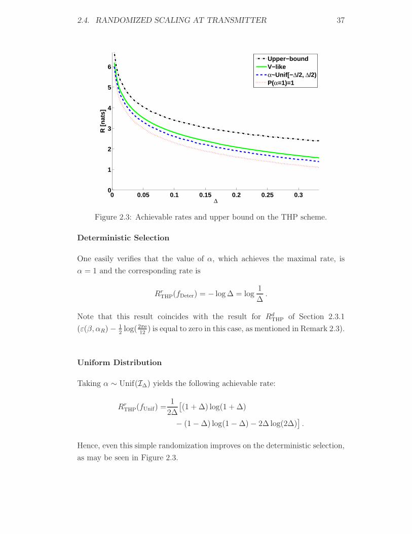
Figure 2.3: Achievable rates and upper bound on the THP scheme.
Deterministic Selection
One easily verifies that the value of α, which achieves the maximal rate, is
α = 1 and the corresponding rate is
RrTHP(fDeter) = − log Δ = log
1
Δ.
Note that this result coincides with the result for RdTHP of Section 2.3.1
(ε(β, αR) − 12log(2πe
12) is equal to zero in this case, as mentioned in Remark 2.3).
Uniform Distribution
Taking α ∼ Unif(IΔ) yields the following achievable rate:
RrTHP(fUnif) =
1
2Δ
[(1 + Δ) log(1 + Δ)
− (1 − Δ) log(1 − Δ) − 2Δ log(2Δ)].
Hence, even this simple randomization improves on the deterministic selection,
as may be seen in Figure 2.3.

38 CHAPTER 2. ROBUSTNESS OF DIRTY PAPER CODING
V-like Distribution
A further improvement is obtained by taking a V-like distribution,
fV−like(α) =|α− 1|
Δ2, |α− 1| ≤ Δ .
The resulting rate is
RrTHP(fV−like) = − 1
2Δ2
[(1 − Δ2) log(1 − Δ2) + Δ2 log(Δ2)
].
We have not pursued numerical optimization of f(α). We note that none
of the three distributions above are optimal since Iβ(V ;Y ′) varies with β.
Moreover, the optimal p.d.f. will not be totally symmetric around 1 due to the
denominator in (2.8). This term becomes, however, less and less significant
(and hence the optimal p.d.f. more and more symmetric) for small Δ. We
next derive an upper bound on the achievable rate which holds for any choice
of f(α).
2.4.2 Upper Bound on Achievable Rates
Lemma 2.3. The rate achievable using THP with randomized scaling is upper
bounded by
RrTHP ≤ log(1 + Δ) − log(Δ) + 1
for any distribution f(α), when Δ ≤ 13.
Proof. Using (2.8), for every distribution f(α), we have
Iβ(V ;Y ′) = minβ
{Eα [logα] −Eα [log |α− β|]}(a)
≤ minβ
{log(1 + Δ) −Eα [log(|α− β| mod Λ)]}
(b)
≤ log(1 + Δ) − 1
2Δ
∫ Δ
−Δ
log |x|dx
= log(1 + Δ) − log(Δ) + 1,
where (a) holds since Supp {f(α)} ⊆ IΔ and (b) is true due to the monotonicity

2.4. RANDOMIZED SCALING AT TRANSMITTER 39
of the log function where equality is achieved for α ∼ Unif(IΔ).
2.4.3 Noisy Case
The randomized approach taken may be extended to the noisy case:
Y ′ =[v +Nβ
eff
]mod Λ ,
Nβeff = (1 − αR)U +
(αR − β
α
)S
β+ αRN.
This result is easily obtained by substituting αT = 1/α in (2.2).
Consider the case of SIR → 0 (and finite SNR). In this case αR has to
be chosen to be equal to β/α, in order to eliminate the residual interference
component in the effective noise. The effective noise in this case is hence:
Nβeff =
α− β
αU +
β
αN.
Note that, unlike in the noiseless case, in which the effective noise had
only a finite support (“self-noise”) component α−βαU , here the noise has an
additional Gaussian component βαN .
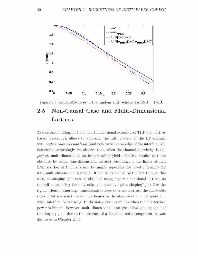
We only examine the deterministic and uniform distributions from Chap-
ter 2.4 and minor variations on them, taking
αT = αMMSE
α� 1
α, where α is selected according to the distributions of Chap-
ter 2.4 and αMMSE � SNR1+SNR
. The performances of the different choices of αT
are shown in Figure 2.4.
Note that in the high SNR regime, the non-deterministic distributions prove
to be more effective than the best deterministic scheme, whereas in the low
SNR regime the deterministic selection becomes superior. This threshold phe-
nomenon can be explained by considering the two components of Nβeff: in the
high SNR regime, the dominant noise component is the “self-noise” compo-
nent α−βαU , which is minimized by a “smart” selection of f(·); in the low SNR
regime, on the other hand, the dominant noise component is the Gaussian
part βαN , whose multiplicative factor β
αshould be deterministic to minimize
its average power. In general, there is a tradeoff between the best deterministic
selection of αT which minimizes the power of the Gaussian component and the
self-noise component, which is to be minimized by a random αT selection.
40 CHAPTER 2. ROBUSTNESS OF DIRTY PAPER CODING
0 0.05 0.1 0.15 0.2 0.25 0.30.4
0.6
0.8
1
1.2
1.4
1.6
Δ
R [
nat
s]
α=1α=α
MMSE
Unif[1−Δ,1+Δ]Unif[α
MMSE(1−Δ),α
MMSE(1+Δ)]
Figure 2.4: Achievable rates in the random THP scheme for SNR = 17dB.
2.5 Non-Causal Case and Multi-Dimensional
Lattices
As discussed in Chapter 1.4.3, multi-dimensional extension of THP (i.e., lattice-
based precoding), allows to approach the full capacity of the DP channel
with perfect channel knowledge (and non-causal knowledge of the interference).
Somewhat surprisingly, we observe that, when the channel knowledge is im-
perfect, multi-dimensional lattice precoding yields identical results to those
obtained by scalar (one-dimensional lattice) precoding, in the limits of high
SNR and low SIR. This is seen by simply repeating the proof of Lemma 2.2
for a multi-dimensional lattice Λ. It can be explained by the fact that, in this
case, no shaping gain can be obtained using higher dimensional lattices, as
the self-noise, being the only noise component, “gains shaping” just like the
signal. Hence, using high-dimensional lattices does not increase the achievable
rates of lattice-based precoding schemes in the absence of channel noise and
when interference is strong. In the noisy case, as well as when the interference
power is limited, however, multi-dimensional strategies allow gaining some of
the shaping gain, due to the presence of a Gaussian noise component, as was
discussed in Chapter 2.4.3.
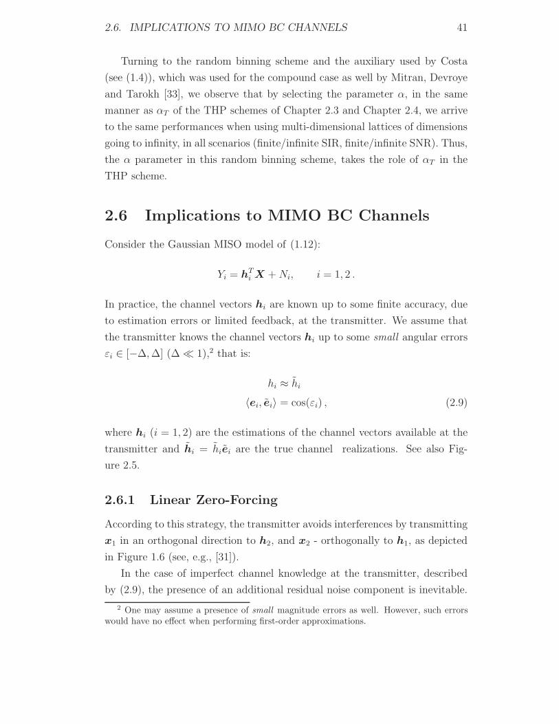
2.6. IMPLICATIONS TO MIMO BC CHANNELS 41
Turning to the random binning scheme and the auxiliary used by Costa
(see (1.4)), which was used for the compound case as well by Mitran, Devroye
and Tarokh [33], we observe that by selecting the parameter α, in the same
manner as αT of the THP schemes of Chapter 2.3 and Chapter 2.4, we arrive
to the same performances when using multi-dimensional lattices of dimensions
going to infinity, in all scenarios (finite/infinite SIR, finite/infinite SNR). Thus,
the α parameter in this random binning scheme, takes the role of αT in the
THP scheme.
2.6 Implications to MIMO BC Channels
Consider the Gaussian MISO model of (1.12):
Yi = hTi X +Ni, i = 1, 2 .
In practice, the channel vectors hi are known up to some finite accuracy, due
to estimation errors or limited feedback, at the transmitter. We assume that
the transmitter knows the channel vectors hi up to some small angular errors
εi ∈ [−Δ,Δ] (Δ � 1),2 that is:
hi ≈ hi
〈ei, ei〉 = cos(εi) , (2.9)
where hi (i = 1, 2) are the estimations of the channel vectors available at the
transmitter and hi = hiei are the true channel realizations. See also Fig-
ure 2.5.
2.6.1 Linear Zero-Forcing
According to this strategy, the transmitter avoids interferences by transmitting
x1 in an orthogonal direction to h2, and x2 - orthogonally to h1, as depicted
in Figure 1.6 (see, e.g., [31]).
In the case of imperfect channel knowledge at the transmitter, described
by (2.9), the presence of an additional residual noise component is inevitable.
2 One may assume a presence of small magnitude errors as well. However, such errorswould have no effect when performing first-order approximations.
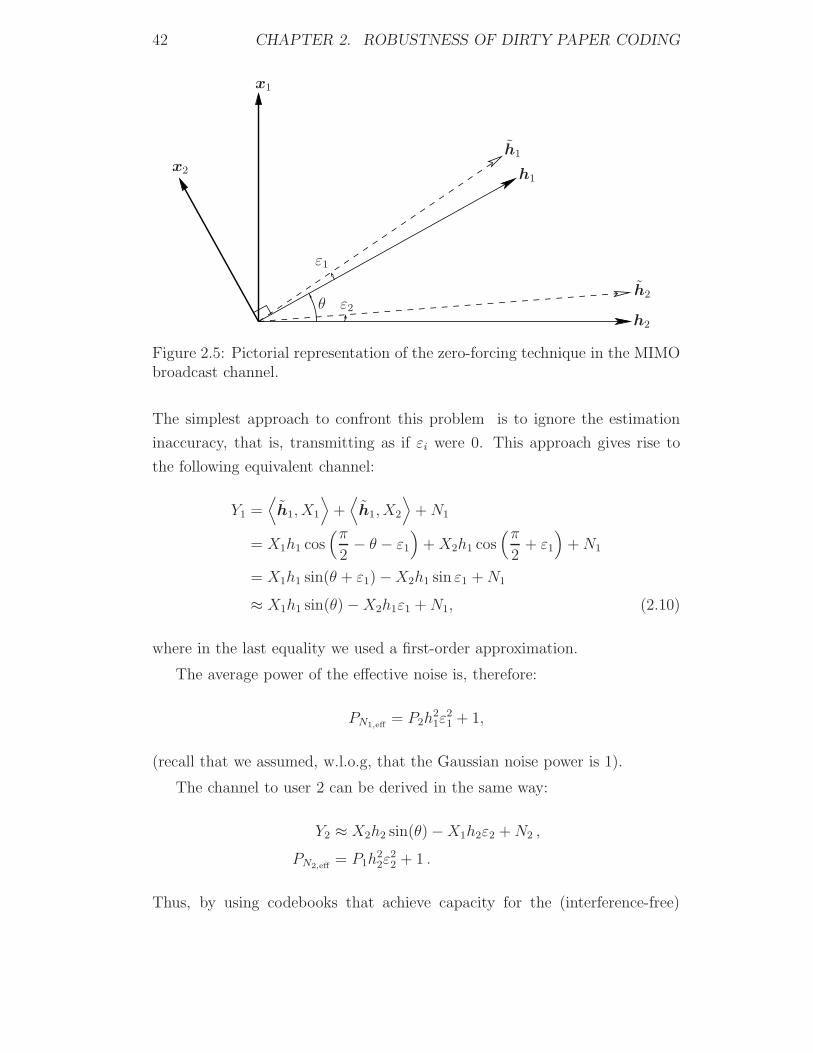
42 CHAPTER 2. ROBUSTNESS OF DIRTY PAPER CODING
θ
ε1
ε2
h1
h2
h1
h2
x1
x2
Figure 2.5: Pictorial representation of the zero-forcing technique in the MIMObroadcast channel.
The simplest approach to confront this problem is to ignore the estimation
inaccuracy, that is, transmitting as if εi were 0. This approach gives rise to
the following equivalent channel:
Y1 =⟨h1, X1
⟩+⟨h1, X2
⟩+N1
= X1h1 cos(π
2− θ − ε1
)+X2h1 cos
(π2
+ ε1
)+N1
= X1h1 sin(θ + ε1) −X2h1 sin ε1 +N1
≈ X1h1 sin(θ) −X2h1ε1 +N1, (2.10)
where in the last equality we used a first-order approximation.
The average power of the effective noise is, therefore:
PN1,eff= P2h
21ε
21 + 1,
(recall that we assumed, w.l.o.g, that the Gaussian noise power is 1).
The channel to user 2 can be derived in the same way:
Y2 ≈ X2h2 sin(θ) −X1h2ε2 +N2 ,
PN2,eff= P1h
22ε
22 + 1 .
Thus, by using codebooks that achieve capacity for the (interference-free)

2.6. IMPLICATIONS TO MIMO BC CHANNELS 43
AWGN channel, any rate pair (R1, R2) satisfying:
R1 ≤1
2log
(1 +
SNR1h21 sin2(θ)
SNR2h21Δ
2 + 1
)− o(1)
R2 ≤1
2log
(1 +
SNR2h22 sin2(θ)
SNR1h22Δ
2 + 1
)− o(1) (2.11)
is achievable, under first-order approximations (Δ � 1), where o(1) → 0 as
Δ → 0.
We suggest improving the above scheme by working matched to the case
of h1 tilted by an additional angle of our choice, when sending x2. That is,
sending x2 in an orthogonal direction to h1 after subtracting a small angle α1.
As the scheme is symmetric for both users, we apply the same strategy in the
transmission direction of x1, by subtracting a small angle α2.
Repeating the steps of (2.10), we arrive to the channel
Y1 ≈ X1h1 sin(θ) +X2h1(α1 − ε1) +N1,
where again, first-order approximation is assumed. As in Chapter 2.4, we
shall allow the use of a random selection of α1, according to some marginal
distribution f(α1). Hence, the (worst-case) achievable rates in this case are:
R1 = maxf(α1)
minε1∈[−Δ,Δ]
I(X1 ;Y1|α1)
≈ maxf(α1)
minε1
Eα1
1
2log
(1 +
SNR1h21 sin2(θ)
SNR2h21(α1 − ε1)2 + 1
),
R2 ≈ maxf(α2)
minε2
Eα2
1
2log
(1 +
SNR2h22 sin2(θ)
SNR1h22(α2 − ε2)2 + 1
). (2.12)
Similarly to the optimization problem of (2.8), the maximization problems
in (2.12) are convex. Thus, the expressions in (2.12) are maximized for
non-deterministic selections of α1 and α2.
2.6.2 Dirty Paper Coding
We now address the problem of working with DPC based schemes, when the
channel knowledge is imperfect and given in the form of (2.9). We analyze

44 CHAPTER 2. ROBUSTNESS OF DIRTY PAPER CODING
θ
ε1
ε2
h1
h2
h1
h2
x1
x2
Figure 2.6: Pictorial representation of the DPC technique for the MIMO broad-cast channel.
the performance of this scheme for the imperfect case, by repeating the steps
in the treatment of the perfect knowledge case, described in Chapter 1.4.6.
We distinguish between the inflation factors at the transmitter, αT , and the
receiver, αR, as explained in Chapter 2.3.1, to facilitate the treatment for
different approaches, similar to the ones discussed for the channel in (2.1)
earlier in this section.
The channel to user 1 (the user that performs DPC), is (see also Figure 2.6):
Y1 =⟨h1,X1
⟩+⟨h1,X2
⟩+N1
= X1h1 cos(π
2− θ − ε1
)+X2h1 cos(θ + ε1) +N1
= X1h1 sin(θ + ε1) +X2h1 cos(θ + ε1) +N1 ,
or equivalently, after dividing both sides by h1 sin(θ + ε1)
Y1 = X1 + ctg(θ + ε1)X2 +1
h1 sin(θ + ε1)N1 .
By constructing the coding scheme, similarly to the one in (1.16), we arrive to
the (lattice) modulo-additive channel, of the form:
X1 = [v1 − αT ctg(θ)X2 − U ] mod Λ ,
2.6. IMPLICATIONS TO MIMO BC CHANNELS 45
Y ′1 =
[αRY1 + U
]mod Λ
=[v1 +N ε1
1,eff
]mod Λ ,
where
N ε11,eff = −(1 − αR)X1 +
(αRctg(θ + ε1) − αT ctg(θ)
)X2
+αR
h1 sin(θ + ε1)N1 . (2.13)
Let us concentrate on the case in which 1 � P1 � P2, that is, the case
in which the interference (the message to user 2) is much stronger than the
power of user 1 and both SNRs are high; we shall further assume that the angle
between the two channel vectors satisfies θ < (π/2 − Δ), since otherwise dirty
paper coding is unattractive as explained in Remark 2.2.1., and also assume
that 0 < Δ � θ, since otherwise the directions of the two channel vectors are
virtually indistinguishable. Note that this means that we continue to assume
small “error intervals”, viz., Δ � 1, like was done for the linear ZF strategy.
Taking the naıve approach, viz., ignoring the imperfectness in the channel
knowledge, suggests working with αR = αT ≈ 1, as the SNRs are high. Thus,
the effective noise in (2.13) is equal, under first order approximation, to:
N ε1
1,eff ≈ −X2 csc2(θ)ε1 +1
h1 sin(θ)N1 ,
where csc(x) � 1/ sin(x).
Note also, that the channel seen by user 2, in this case, is the same as in
the linear ZF scheme. Hence, using the “naıve” approach, we achieve any rate
pair (R1, R2), satisfying:
R1 ≤1
2log
(1 +
SNR1h21 sin2(θ)
SNR2h21 csc2(θ)Δ2 + 1
)− o(1) ,
R2 ≤1
2log
(1 +
SNR2h22
SNR1h22Δ
2 + 1
)− o(1) , (2.14)
where o(1) → 0 as Δ → 0.
We now move to examining the performance of the “smart receiver” (see Chap-
ter 2.3.3) system, which uses the same transmitter as in the “naıve” approach,

46 CHAPTER 2. ROBUSTNESS OF DIRTY PAPER CODING
and a receiver which performs MMSE estimation, to compensate for the ad-
ditional ε1 factor. Since we assumed 1 � P1 � P2, the inflation factor at
the transmitter is αT ≈ 1 and the receiver ought to eliminate any residual
interference by selecting
αR = tg(θ + ε1)ctg(θ)αT ≈ tg(θ + ε1)ctg(θ) .
By using first-order approximations (Δ � 1), we arrive to the following ex-
pression for the effective noise:
N ε11,eff ≈ 2X2 csc(2θ)ε1 +
1
h1 sin(θ)N1 ,
Again, since user 2, sees the same channel as in the linear ZF scheme, the
following rates are achievable:
R1 ≤1
2log
(1 +
SNR1h21 sin2(θ)
SNR1h21 sec2(θ)Δ2 + 1
)− o(1)
R2 ≤1
2log
(1 +
SNR2h22
SNR1h22Δ
2 + 1
)− o(1) , (2.15)
where again o(1) → 0 as Δ → 0.
Finally, we introduce randomization at the transmission, in the form of a
random inflation factor αT for user 1 (the one that performs DPC), to assist
in enlarging its own rate (R1), and “the same” angular fluctuation to the
transmission directions of both users. The perturbations in the transmission
direction of user 1, improves the performance of user 2, just like in the linear
ZF case. The fluctuation in the transmission direction of user 2, causes no
additional (first order) improvement, nevertheless, tilting both vectors (t1 and
t2) by the same angle, facilitates in the choice of the two fluctuations, as will
become apparent in the sequel. We denote by α2 the angular perturbations
of t1 and t2, and by α1 - the perturbation in the amplitude of user 1 (in the
inflation factor of x1).
The channel to user 1, in this case, is therefore
Y1 =⟨h1,X1
⟩+⟨h1,X2
⟩+N1
= X1h1 cos(π
2− θ − (ε1 − α2)
)+X2h1 cos(θ + (ε1 − α2)) +N1

2.6. IMPLICATIONS TO MIMO BC CHANNELS 47
= X1h1 sin(θ + (ε1 − α2)) +X2h1 cos(θ + (ε1 − α2)) +N1 ,
and after dividing by h1 sin(θ + ε1 − α2):
Y1 = X1 + ctg(θ + ε1 − α2)X2 +1
h1 sin(θ + ε1 − α2)N1 .
The (lattice) modulo-additive channel, in this case, is:
X1 = [v1 − ctg(θ − α2 + α1)X2 − U ] mod Λ ,
Y ′1 = [αRy1 + U ] mod Λ
=[v1 +N ε1
1,eff
]mod Λ ,
where
N ε1
1,eff = −(1 − αR)X1 +(αRctg(θ + ε1 − α2)X1 − ctg(θ − α2 + α1)
)X2
+αR
h1 sin(θ + ε1 − α2)N1
≈ 2 csc(2θ)(ε1 − α1)X1 +1
h1 sin(θ)N1 , (2.16)
and (2.16) holds under first order approximation and the choice
αR = ctg(θ − α2α1)tg(θ + ε1 − α2), which eliminates any residual interfer-
ence.
This implicates the achievability of any rate pair (R1, R2) satisfying:
R1 ≤ maxf(α1)
minε1
Eα1
1
2log
(1 +
SNR1h21 sin2(θ)
SNR1h21 sec2(θ)(α1 − ε1)2 + 1
)− o(1)
R2 ≤ maxf(α2)
minε2
Eα2
1
2log
(1 +
SNR2h22
SNR1h22(α2 − ε2)2 + 1
)− o(1) , (2.17)
where o(1) → 0 as Δ → 0.
Just like in (2.12), the maximization problems in (2.17) are convex, which
means that non-deterministic selections of α1 and α2 need to be made to
achieve optimum.
Remark 2.5.
• The intervals of uncertainty might be of different size, i.e., Δ1 �= Δ2.
Nonetheless, the treatment in this section is easily extended to this case.

48 CHAPTER 2. ROBUSTNESS OF DIRTY PAPER CODING
• Note that the crosstalk of user 1 in the DPC based scheme (the “weak”
user which performs DPC) depends on the power of this user rather than
the power of user 2, which is the case in the linear ZF approach. Hence,
in the regime P2 � P1, this suggest a great improvement over linear
schemes.
• Comparing the rates achievable by linear ZF, with the ones - via ZF DPC,
that is, (2.11) with (2.15), and (2.12) with (2.17), we see that contrary to
a common belief that the performance of robust DPC rapidly deteriorates
with the growth of uncertainty in the channel coefficients, in many cases
of interest, the opposite is true: for
SNR2 cos2(θ) > SNR1 ,
both the deterministic and the “randomized” DPC schemes, (2.15) and
(2.17), are in fact “more robust” then their linear counterparts, (2.11)
and (2.12). Moreover, by comparing the rates of the “naıve” DPC
scheme (2.14) with the ones of the parallel linear scheme (2.11), we see
that even if the DPC user ignores the fact that there is a lack of channel
knowledge, its performance does not collapse dramatically, and propose
a trade-off between pairs that are achievable using linear schemes and
those which are achievable using DPC.

Chapter 3
Binary Dirty Multiple-Access
Channel
The general two-user memoryless multiple-access channel with com-
mon channel state information among the encoders has no single-
letter solution which explicitly characterizes its capacity region. In
this chapter a binary “dirty” multiple-access channel with interfer-
ence known at both encoders is considered. We derive an achievable
rate region for this channel and determine its sum-rate capacity,
which equals to the capacity when full-cooperation between trans-
mitters is allowed, contrary to the Gaussian case.
3.1 System Model and Motivation
We treat the binary DMAC with non-causal common interference, defined
in Chapter 1.18, to be (see also Figure 1.8):
Y = X1 ⊕X2 ⊕ S ⊕N ,
with input (“power”) constraints 1nwH(xi) ≤ qi. We assume that the interfer-
ence is “strong”, i.e., S ∼ Bernoulli (1/2). This is the worst-case interference
that can be assumed, as any other distribution of the interference can be trans-
formed into this case by incorporating dithering at the receiver’s end.
For simplicity, we concentrate on the “noiseless case” (N = 0).
In Chapter 1.4.2 a method to cancel known interference was discussed. In
49

50 CHAPTER 3. BINARY DIRTY MULTIPLE-ACCESS CHANNEL
the sequel, we use a super-position of such codes along with successive decoding
of the messages (“onion peeling”) and derive an achievable rate region, which
we conjecture to be the capacity region, and is equal to the binary clean MAC
capacity region up to a loss which stems from the loss seen in the point-to-point
case. Moreover, we show that these strategies achieve the sum-rate capacity of
the binary dirty MAC with common interference, which is equal to the capacity
of the clean MAC when full cooperation between the encoders is allowed.
3.2 Clean MAC
In this section we consider the “clean” binary modulo-additive channel:
Y = X1 ⊕X2 ⊕N
with input constraints q1, q2. Note that this channel is identical to our channel
of interest (1.18) up to the interference which is equal to 0 in this case.
The capacity region of this channel contains the capacity region of the our
channel of interest, and therefore serves as an outer bound on its capacity
region. Again, we concentrate on the “noiseless case” (N = 0).
Contrary to the Gaussian case, in which only stationary inputs need to be
considered to achieve capacity, in the binary case, the use of stationary inputs
is not optimal and the convex hull is necessary to achieve the capacity region
envelope. To see this we rewrite (1.17) explicitly for the binary case:
C � cl conv{
(R1,R2) : R1 ≤ Hb(X1)
R2 ≤ Hb(X2)
R1+R2 ≤ Hb(X1 ⊕X2)},
(3.1)
where the closure and the convex hull are taken over all admissible distributions
of the form p1(x1)p2(x2) on {0, 1}× {0, 1} and such that the input constraints
are satisfied.
One easily verifies that, by allowing only stationary inputs in (3.1), .i.e.,

3.2. CLEAN MAC 51
relinquishing the convex hull, the sum-rate R1 +R2 cannot exceed
R1 +R2 ≤ Hb(q1 � q2) . (3.2)
However, as indicated by the following lemma, this is suboptimal.
Lemma 3.1 (Sum-Rate Capacity of the Binary Clean MAC). The sum-rate
capacity of the binary noiseless modulo-additive MAC with input constraints1nwH(xi) ≤ qi, i = 1, 2, is:
Csumclean = H+
b (q1 + q2) , (3.3)
where H+b (q) � Hb
(min
{q, 1
2
}).
Proof. zmbr
Direct: Using time-sharing one can divide each block into two parts: in the
first q1
q2+q2n block samples user 1 spends all of its power to convey his private
message, while user 2 transmits 0, whereas in the remaining q2
q2+q2n block sam-
ples user 2 spends all of its transmission power to convey his message, while
user 1 is silent. Thus in the first q1
q2+q2n samples, user 1 transmits over a bi-
nary (point-to-point) DP channel, whereas in the remaining samples, user 2
transmits over the same DP channel (with a different power constraint). This
leads to the sum-rate
R1 +R2 =q1
q2 + q2H+
b (q1 + q2) +q2
q2 + q2H+
b (q1 + q2)
= H+b (q1 + q2) .
Converse: Allow full cooperation between the transmitters. This can only
increase the sum-rate capacity. Full cooperation transforms the problem into
a point-to-point problem of transmitting over a binary clean channel with
power constraint 1nwH(x) ≤ q1 + q2, the capacity of which is H+
b (q1 + q2).
Thus, the sum-rate capacity of the binary (clean) MAC (3.3) is strictly
greater than the best rate achievable using only stationary inputs (3.2).

52 CHAPTER 3. BINARY DIRTY MULTIPLE-ACCESS CHANNEL
Remark 3.1.
• The sum-rate of the “noisy” clean MAC can be shown, using the same
methods, to be:
Csumclean = H+
b
((q1 + q2) � ε
)−Hb(ε) .
• If we allow full cooperation between the transmitters, the capacity of
the channel does not outperform (3.3), as pointed out in the converse
part of the proof. In the Gaussian case, on the other hand, the sum-rate
capacity of the MAC channel is equal to 12log(1 + SNR1 + SNR2), which
is strictly smaller than the full-cooperation capacity, 12log(1 + SNR1 +
SNR2 + 2√
SNR1SNR2). This dissimilarity stems from the difference of
the alphabets we work with in both problems and the nature of the addi-
tion: in the binary case, no “coherence” can be attained by transmitting
the same message, and additional power can only assist in exploiting
more time slots within a block. In the Gaussian case, on the other hand,
cooperation allows additional coherence gain, which cannot be achieved
otherwise.
To find the capacity region of (3.1) explicitly, we replace the convex hull
with a time-sharing variable Q, with alphabet of size |Q| = 2 (see, e.g., [13]).
C �⋃ {
(R1, R2) : R1 ≤ Hb(X1|Q)
R2 ≤ Hb(X2|Q)
R1+R2 ≤ Hb(X1 ⊕X2|Q)},
(3.4)
where the union is over all admissible Markov chains X1 ↔ Q↔ X2, satisfying
the input constraints EXi ≤ qi, i = 1, 2. The capacity region for q1 = 1/6 and
q2 = 1/10 is depicted in Figure 3.1.
Remark 3.2. Note that X1 and X2 are not independent in (3.4), but rather
independent given the time-sharing parameter Q.
Nonetheless, time-sharing of the form described in the proof of Lemma 3.1
is suboptimal in general, as can be seen in Figure 3.1.
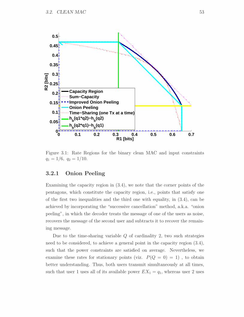
3.2. CLEAN MAC 53
0 0.1 0.2 0.3 0.4 0.5 0.6 0.70
0.05
0.1
0.15
0.2
0.25
0.3
0.35
0.4
0.45
0.5
R1 [bits]
R2
[bit
s]
Capacity RegionSum−CapacityImproved Onion PeelingOnion PeelingTime−Sharing (one Tx at a time)h
b(q1*q2)−h
b(q2)
hb(q2*q1)−h
b(q1)
Figure 3.1: Rate Regions for the binary clean MAC and input constraintsq1 = 1/6, q2 = 1/10.
3.2.1 Onion Peeling
Examining the capacity region in (3.4), we note that the corner points of the
pentagons, which constitute the capacity region, i.e., points that satisfy one
of the first two inequalities and the third one with equality, in (3.4), can be
achieved by incorporating the “successive cancellation” method, a.k.a. “onion
peeling”, in which the decoder treats the message of one of the users as noise,
recovers the message of the second user and subtracts it to recover the remain-
ing message.
Due to the time-sharing variable Q of cardinality 2, two such strategies
need to be considered, to achieve a general point in the capacity region (3.4),
such that the power constraints are satisfied on average. Nevertheless, we
examine these rates for stationary points (viz. P (Q = 0) = 1) , to obtain
better understanding. Thus, both users transmit simultaneously at all times,
such that user 1 uses all of its available power EX1 = q1, whereas user 2 uses

54 CHAPTER 3. BINARY DIRTY MULTIPLE-ACCESS CHANNEL
only some portion of its power EX2 = q′2 (0 ≤ q′2 ≤ q2). User 1 treats q′2 as
noise and can achieve a rate of R1 = Hb(q1 � q′2) − Hb(q′2). After recovering
the message of user 1, it can be subtracted, such that user 2 sees a clean
point-to-point channel and hence can achieve a rate of R2 = Hb(q′2). Note
that even though the capacity region cannot be achieved using this strategy
capacity, it does achieve certain rate pairs which cannot be achieved by simple
time-sharing, like the one used in Lemma 3.1 and depicted in Figure 3.1.
Remark 3.3.
• When using this onion peeling strategy, user 2 does not exploit all of
its power, but only a portion 0 ≤ q′2 ≤ q2. Hence a “residual” power of
q2 − q′2 is left unexploited. This implies that this strategy is not optimal,
as is, and a way to exploit this residual power needs to constructed.
• The roles of user 1 and user 2 are not symmetric: the achievable rate
pairs, using onion peeling, when user 2 is peeled, differ from the rate
pairs that are achieved when user 1 is peeled. Hence, by switching roles
between the two users, one may achieve additional rate points.
3.2.2 Improving the Stationary Onion Peeling
The onion peeling considered in the previous section, can be easily improved,
by dividing each block into two parts (i.e., time-sharing between two strate-
gies): in the first sub-block, onion peeling is applied, whereas in the remaining
time, the user that did not exploit all of its power during the first sub-block
(viz. the onion peeling time period), uses all of its remaining “residual power”,
whereas the other user ought to transmit 0, as he already exploited all of its
power. Let us denote by α the block portion allotted to onion peeling and
by q′2 (0 ≤ q′2 ≤ q2) the power of user 2, used during this period. Hence, the
achievable rates, using this strategy, have the form:
R1 = αH+b
(q1α
� q′2α
)− αH+
b
(q′2α
),
R2 = αH+b
(q′2α
)+ (1 − α)H+
b
(q2 − q′21 − α
), (3.5)

3.3. DIRTY MAC WITH COMMON INTERFERENCE 55
Remark 3.4.
• In the noisy case, one may obtain rate pairs of the form
R1 = αH+b
(q1α
� q′2α
� ε
)− αH+
b
(q′2α
� ε
),
R2 = αH+b
(q′2α
� ε
)+ (1 − α)H+
b
(q2 − q′21 − α
� ε
)−Hb(ε)
in a similar manner.
• Like in “stationary” onion peeling, the roles of the two users are not sym-
metrical. Hence by switching roles between the two users, one achieves
points within the capacity region, that could not be achieved otherwise.
See Remark 3.3.
In fact, by plotting the achievable rate region of this “improved” onion
peeling scheme, for different cases (different {qi} values), 1 we see that it
coincides with the capacity region (3.4). We conjecture that this is always
true and that the capacity region of the binary modulo-additive MAC can be
entirely described by (3.5) (and the symmetric expression in which user 1 and
user 2 switch roles).
3.3 Dirty MAC with Common Interference
We adopt the strategies introduced in Chapter 3.2, to the dirty case, and derive
an achievable rate region.
3.3.1 Sum-Rate Capacity
Similarly to the clean MAC case, the sum-rate capacity of the binary DMAC
with common interference is equal to the capacity of this channel when both
encoders can fully cooperate, as indicated by the following lemma.
Lemma 3.2 (Sum-Rate Capacity of DMAC with Common SI). The sum-
rate capacity of the binary noiseless modulo-additive dirty MAC with common
1We do so for both when user 2 is peeled first and when user 2 is peeled first.

56 CHAPTER 3. BINARY DIRTY MULTIPLE-ACCESS CHANNEL
interference and input constraints 1nwH(xi) ≤ qi, i = 1, 2, is:
Csumdirty = H+
b (q1 + q2) . (3.6)
Proof. zmbr
Direct: We repeat the proof of Lemma 3.1, only now the point-to-point BSC
capacity (1.6) should be replaced by the binary DP channel capacity (1.5).
Nevertheless, in the noiseless case (N = 0), there is no difference between the
two expressions, and thus
R1 +R2 = H+b (q1 + q2) .
Converse: Again, like in the proof of Lemma 3.1, we allow full cooperation
between the transmitters, which in turn transforms the problem into a point-
to-point channel, the capacity of which is H+b (q1 + q2).
Remark 3.5.
• In the presence of noise, the sum-rate capacity of this channel is
CsumDirty = uch max
{H+
b (q1 + q2) − Hb(ε), 0}.
• In the noiseless case, the sum-rate capacities of the binary clean and
dirty MACs are equal. However, in the presence of noise N , the sum-
rate capacity of the dirty MAC channel is strictly smaller than that of
the clean MAC channel (for q1 + q2 <12). This difference stems from the
capacity loss, due to the presence of interference. in the point-to-point
setting, as discussed in Chapter 1.4.2.
• As was mentioned in Remark 3.1, if we allow full cooperation between
the transmitters, the capacity of the channel cannot exceed (3.6), in
contrast to the Gaussian case, in which additional “coherence gain” can
be achieved.
3.3.2 Onion Peeling
The capacity region of the “single informed user” (see Chapter 1.4.8) serves
as an inner bound for the capacity region of the common interference dirty

3.3. DIRTY MAC WITH COMMON INTERFERENCE 57
MAC. To improve the achievable region of our channel of interest, we allow
time-sharing between “single informed user” strategies, where the informed
user is alternately user 1 and user 2.
The strategies used by Philosof, Zamir and Erez [37] to achieve the capacity
region of the single informed user (1.19), can be viewed as onion peeling, where
user 2 transmits in the same way, as described in Chapter 3.2.1, i.e., assumes
a clean channel and input constraint 0 ≤ q′2 ≤ q2; and user 1 treats the signal
of user 2, X2, as noise and uses dirty paper coding of the form (1.5). The
achievable rates, using this strategy, are of the form:
R1 = Hb(q1) −Hb(q′2) ,
R2 = Hb(q′2) ,
where since q′2 can take any value in the interval [0, q2], the single informed
user capacity (1.19) is achieved by time-sharing between such strategies.
Remark 3.6.
• Using such “stationary”strategy alone (with no time-sharing), one can-
not hope to achieve the sum-rate capacity of Lemma 3.2 (or the whole
capacity region of the single-informed user problem (1.19)).
• As in Remark 3.3, there is an average residual power of q2 − q′2, for each
sample, left unexploited.
• This strategy is asymmetric in user 1 and user 2, as was explained in Re-
mark 3.3.
3.3.3 Improved Onion Peeling
As was done for the clean MAC in Chapter 3.2.2, we improve the achievable
rate region of “stationary” onion peeling, by employing time-sharing between
an onion peeling strategy (discussed in Chapter 3.3.2) and transmission of the
residual power (where the other user is silent). This allows to achieve rate
pairs of the form:
R1 = αH+b
(q1α
)− αH+
b
(q′2α
),
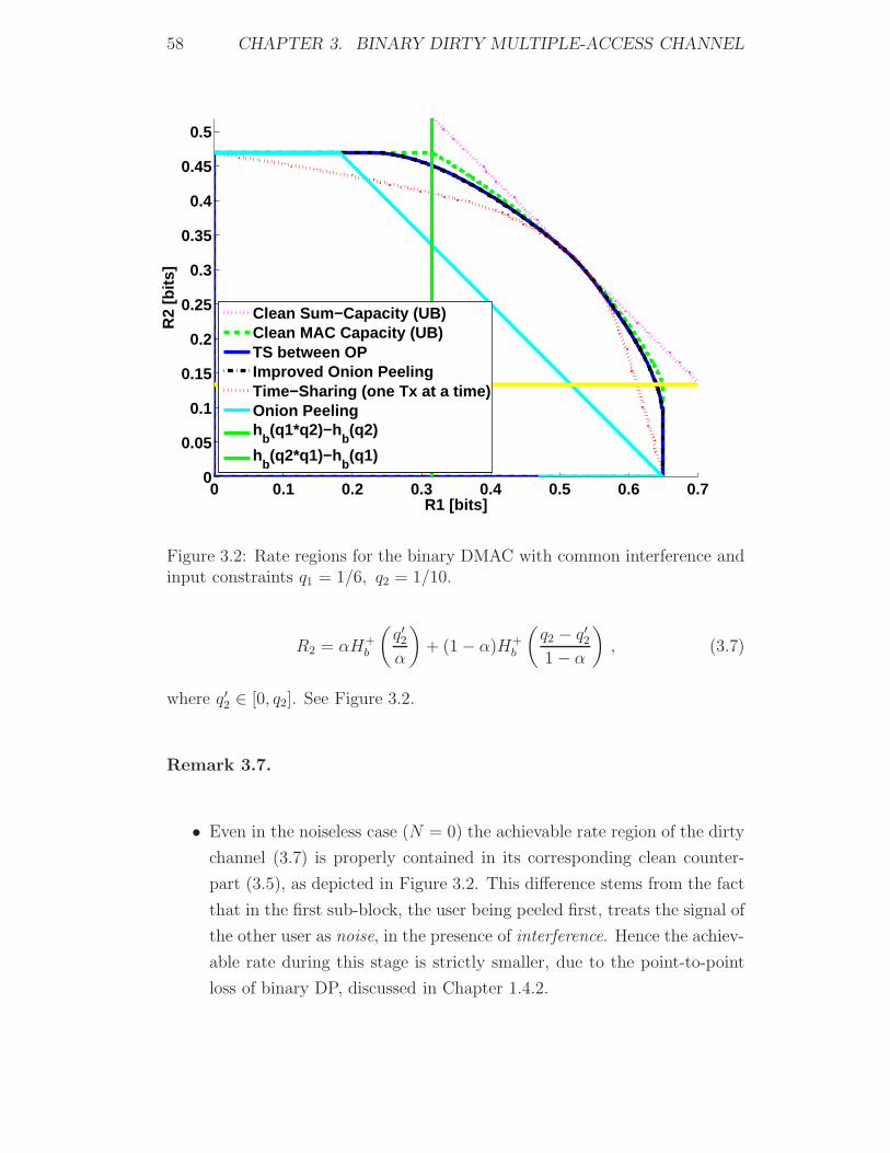
58 CHAPTER 3. BINARY DIRTY MULTIPLE-ACCESS CHANNEL
0 0.1 0.2 0.3 0.4 0.5 0.6 0.70
0.05
0.1
0.15
0.2
0.25
0.3
0.35
0.4
0.45
0.5
R1 [bits]
R2
[bit
s]
Clean Sum−Capacity (UB)Clean MAC Capacity (UB)TS between OPImproved Onion PeelingTime−Sharing (one Tx at a time)Onion Peelingh
b(q1*q2)−h
b(q2)
hb(q2*q1)−h
b(q1)
Figure 3.2: Rate regions for the binary DMAC with common interference andinput constraints q1 = 1/6, q2 = 1/10.
R2 = αH+b
(q′2α
)+ (1 − α)H+
b
(q2 − q′21 − α
), (3.7)
where q′2 ∈ [0, q2]. See Figure 3.2.
Remark 3.7.
• Even in the noiseless case (N = 0) the achievable rate region of the dirty
channel (3.7) is properly contained in its corresponding clean counter-
part (3.5), as depicted in Figure 3.2. This difference stems from the fact
that in the first sub-block, the user being peeled first, treats the signal of
the other user as noise, in the presence of interference. Hence the achiev-
able rate during this stage is strictly smaller, due to the point-to-point
loss of binary DP, discussed in Chapter 1.4.2.
3.3. DIRTY MAC WITH COMMON INTERFERENCE 59
• In the noisy case, one may obtain rate pairs of the form
R1 = αH+b
(q1α
)− αH+
b
(q′2α
� ε
),
R2 = αH+b
(q′2α
� ε
)+ (1 − α)H+
b
(q2 − q′21 − α
� ε
)−Hb(ε)
in a similar manner.
• The roles of the two users are not symmetrical. Hence by switching roles
between the two users, one achieves points within the capacity region,
that could not be achieved otherwise. See Remark 3.3.
One could suspect that allowing time-sharing between a few onion peeling
strategies can further improve this region. Nevertheless, by plotting the corre-
sponding rate region (see Figure 3.2), one sees that no further improvement is
gained this way. Thus, we conjecture, like for the clean MAC, that strategies of
the form (3.7), are in fact sufficient to achieve any point in the capacity region
of the binary DMAC with common interference. Nevertheless, the problem of
determining the capacity region of this problem remains open.

Chapter 4
Summary
In this work, the compound dirty-paper channel was considered. The capacity
of general compound channels with causal side information was determined.
We further studied the performance that may be achieved for the specific case
of the DP channel model by an extended Tomlinson-Harashima precoding
scheme and derived lower bounds on the capacity of the channel. We derived
the MMSE scaling that can be applied at the receiver to compensate for impre-
cise channel knowledge at the transmitter. We further showed that randomized
inflation scaling at the transmitter may further improve the achievable rate.
We also showed that the potential shaping gain of higher lattice dimensions
diminishes with the increase of the channel estimation inaccuracy and that
well designed dirty paper coding techniques for the MIMO broadcast channel
can be even more robust than their linear counterparts.
This work focused exclusively on the performance achievable using THP-
like schemes. It would be interesting to obtain an upper bound on the capacity
(without any restriction on the coding technique) for the noiseless DP channel
under channel uncertainty.
In the second part of this work, we studied the binary dirty multiple-access
channel with common interference. We first studied the clean binary multiple-
access channel. Using our understanding of the clean multiple-access channel,
we were able to derive the sum-rate capacities of both the clean and the dirty
MAC, which were shown to be equal to the capacities of these channels when
full cooperation between the encoders is allowed. We also derived an achievable
rate region for the clean and the dirty multiple-access channels and conjectured
60

61
that the capacities of both of these channels can be described in a simple
manner, which corresponds to a simple successive decoding technique.

Appendix A
A.1 Proof of Theorem 2.1
Direct. Denote by T the family of all mappings from S to X . Use a transmitter
that sends x = t(s), where t is chosen in an i.i.d. manner, according to some
predefined probability distribution p(t). In this case, the problem reduces to
that of a compound channel with no side information, with an input alphabet
T (see [42]), the same output alphabet Y and the corresponding transition
probabilities
p(y|t) =∑s∈S
p(y|x = t(s), s) .
Hence, by maximizing over all possible input probabilities, p(t), of the equiv-
alent channel, we have an inner bound on the (worst-case) capacity (see, e.g.,
[4]):
C ≥ p(t) ∈ P(T ) infβ∈B
Iβ(T ;Y ) .
Converse. For each n, let the information message W be drawn according
to a uniform distribution over {1, ..., 2nR}. Denote the error probability cor-
responding to β ∈ B by P(n)e,β and the error probability of the scheme as the
supremum of these probabilities, P(n)e �
∑β∈B P
(n)e,β . Then we have:
nR = H(W ) ≤ 1 + P(n)e,β nR + Iβ(W ;Y n
1 )
≤ 1 + P (n)e nR +
n∑i=1
Iβ(W ;Yi|Y i−11 ) ,
62

A.2. PROOF OF LEMMA 2.2 AND TREATMENT FOR Δ > 1/3 63
where the first inequality is due to Fano’s inequality (see, e.g., [12]) and the
second inequality follows from the chain-rule for mutual information. By re-
tracing the steps of Shannon in [42], we have Iβ(W ;Yi|Y i−11 ) ≤ Iβ(W,Si−1
1 ;Yi),
for every β ∈ B. Since{W,Si−1
1
}does not depend on the value of β, the
following inequality holds true as explained in detail in [42]:
nR ≤ P (n)e nR +
n∑i=1
Iβ(Ti;Yi), ∀β ∈ B .
The inequality above needs to be held for all β ∈ B simultaneously, and hence
can be rewritten as
nR ≤ maxp(t)∈P(T )
infβ∈B
P (n)e nR + nIβ(T ;Y ) .
Finally, dividing by n, taking Pe → 0 and letting n→ ∞, we obtain
R ≤ maxp(t)∈P(T )
infβ∈B
Iβ(T ;Yi) .
A.2 Proof of Lemma 2.2 and treatment for
Δ > 1/3
Proof of Lemma 2.2. The term
Iβ(V ;Y ′|α) = hβ(Y ′|α) − hβ(Y ′|V, α)
is maximized by taking V ∼ Unif(Λ). Moreover, it is easily seen that the
support of f(α) should be restricted to IΔ. It follows that,
Iβ(V ;Y ′|α) = hβ(Y ′|α) − hβ(Y ′|V, α)
= log(L) − hβ(Y ′|V, α)
= log(L) − h([Nβeff] mod Λ)
= log(L) − Eα
[h
([α− β
αU
]mod Λ
)].

64 APPENDIX A.
The term α−βα
is maximized when α = 1 − Δ and β = 1 + Δ, and is equal to2Δ
1−Δ. Hence, for Δ ≤ 1
3, we have α−β
α≤ 1. Therefore,
Iβ(V ;Y ′|α) = log(L) − Eα
[h
(α− β
αU
)]
= log(L) + Eα
[− log(Δ) − log
∣∣∣∣α− β
α
∣∣∣∣]
= −Eα log
∣∣∣∣α− β
α
∣∣∣∣ .
The case of Δ > 1/3 can be treated in a similar manner by employing the
following lemma.
Lemma A.1. Suppose U ∼ Unif(V0). Then for every a > 1, the entropy of([aU ] mod Λ
)is bounded by
log(L) − log
(�a�a
)≤ h([aU ] mod Λ) ≤ log(L) .
Proof. The upper-bound follows easily from the fact that differential entropy is
maximized by a uniform distribution, when subject to an amplitude constraint,
see, e.g. [12]. To prove the lower-bound, note that there is a unique index k ∈ Z
which satisfies
aU = [aU ] mod Λ + kL,
with alphabet cardinality |K| = �a�. One may easily verify [39], that the
following relation holds
h(aU) = h([aU ] mod Λ) +H(k|[aU ]) ,
which leads to the desired bound:
h([aU ] mod Λ) = log(aL) −H(k|[aU ])
≥ log(aL) −H(k)
= log(aL) − log(a+ 1)

A.2. PROOF OF LEMMA 2.2 AND TREATMENT FOR Δ > 1/3 65
= log(L) − log
(�a�a
).

Bibliography
[1] R. Ahlswede. Multi-way communication channels. In Proceedings of 2nd
International Symposium on Information Theory, Thakadsor, Armenian
S.S.R., Sept. 1971. Akademiai Kiado, Budapest, 1973, pages 23–52.
[2] R. J. Barron, B. Chen, and G. W. Wornell. The duality between in-
formation embedding and source coding with side information and some
applications. IEEE Trans. Information Theory, 49:1159–1180, May 2003.
[3] A. Bennatan, V. Aggarwal, Y. Wu, A. R. Calderbank, J. Hoydis, and
A. Chindapol. Bounds and lattice-based transmission strategies for the
phase-faded dirty-paper channel. IEEE Trans. Wireless Communications.
[4] D. Blackwell, L. Breiman, and A. J. Thomasian. The capacity of a class
of channels. The Annals of Mathematical Statistics, 30:1229–1241, Dec.
1959.
[5] G. Caire, N. Jindal, M. Kobayashi, and N. Ravindran. Quantized vs.
analog feedback for the MIMO broadcast channel: A comparison between
zero-forcing based achievable rates. In Proc. Int. Symp. Inform. Theory
(ISIT), Nice, France, pages 2046–2050, June 2007.
[6] G. Caire and S. Shamai (Shitz). On the achievable throughput of a multi-
antenna Gaussian broadcast channel. IEEE Trans. Information Theory,
IT–49:1649–1706, July 2003.
[7] B. Chen and G. W. Wornell. Quantization index modulation: A class of
provably good methods for digital watermarking and information embed-
ding. IEEE Trans. Information Theory, IT–47:1423–1443, May 2001.
66

BIBLIOGRAPHY 67
[8] R. Chen, R.W. Heath Jr., and J.G. Andrews. Transmit selection diversity
for unitary precoded multiuser spatial multiplexing systems with linear
receivers. IEEE Trans. Signal Processing, vol. 55, no. 3.
[9] A. S. Cohen and A. Lapidoth. The Gaussian watermarking game. IEEE
Trans. Information Theory, June, 2002, 1639–1667. See also, On the Gaus-
sian Watermarking Game, Proc. Int. Symp. Inform. Theory (ISIT), page
48, Sorrento, Italy, June 2000.
[10] J. H. Conway and N. J. A. Sloane. Sphere Packings, Lattices and Groups.
Springer-Verlag, New York, N.Y., 1988.
[11] M. H. M. Costa. Writing on dirty paper. IEEE Trans. Information Theory,
IT-29:439–441, May 1983.
[12] T. M. Cover and J. A. Thomas. Elements of Information Theory. Wiley,
New York, 1991.
[13] I. Csiszar and J. Korner. Information Theory - Coding Theorems for
Discrete Memoryless Systems. Academic Press, New York, 1981.
[14] R. L. Dobrushin. Optimal information transmission over a channel with
unknown parameters (in Russian). Radiotekh. i Elektron., Vol. 4, No.
12:1961–1956, Dec. 1959.
[15] J. J. Eggers, R. Baumel, R. Tzschoppe, and B. Girod. Scalar Costa
scheme for information embedding. IEEE Trans. Signal Processing, pages
1003–1019, Apr., 2003.
[16] U. Erez, S. Litsyn, and R. Zamir. Lattices which are good for (almost) ev-
erything. IEEE Trans. Information Theory, IT-51:3401–3416, Oct. 2005.
[17] U. Erez, S. Shamai (Shitz), and R. Zamir. Capacity and lattice strategies
for cancelling known interference. IEEE Trans. Information Theory, pages
3820–3833, Nov. 2005.
[18] G. D. Forney, Jr. On the role of MMSE estimation in approaching the
information- theoretic limits of linear Gaussian channels: Shannon meets
Wiener. In 41st Annual Allerton Conference on Communication, Control,

68 BIBLIOGRAPHY
and Computing, Allerton House, Monticello, Illinois, pages 430–439, Oct.
2003.
[19] S. I. Gel’fand and M. S. Pinsker. Coding for channel with random pa-
rameters. Problemy Pered. Inform. (Problems of Inform. Trans.), 9, No.
1:19–31, 1980.
[20] S. I. Gel’fand and M. S. Pinsker. On Gaussian channels with random pa-
rameters. In Abstracts of Sixth International Symposium on Information
Theory, Tashkent, U.S.S.R, pages 247–250, Sep. 1984.
[21] P. Grover and A. Sahai. What is needed to exploit knowledge of primary
transmissions? available at arXiv:cs/0702071.
[22] H. Harashima and H. Miyakawa. Matched-transmission technique for
channels with intersymbol interference. IEEE Trans. Communications,
COM-20:774–780, Aug. 1972.
[23] S. A. Jafar. Capacity with causal and non-causal side information - a
unified view. IEEE Trans. Information Theory, IT-52:5468–5475, Dec.
2006.
[24] N. Jindal. MIMO broadcast channels with finite-rate feedback. IEEE
Trans. Information Theory, Vol. 52, No. 11:5045–5060, Nov. 2003.
[25] A. Khina and U. Erez. On the robustness of dirty paper coding. IEEE
Trans. Communications, IT-58, accepted for publication, May 2010.
[26] A. Khina and U. Erez. On robust dirty paper coding. In Proceedings of
IEEE Information Theory Workshop, ITW 2008, Porto, Portugal, pages
204–208, May 2008.
[27] Y. H. Kim, A. Sutivong, and S. Sigurjonsson. Multiple user writing on
dirty paper. In Proceedings of IEEE International Symposium on Infor-
mation Theory, Chicago, USA, June 2004.
[28] S. Kotagiri and J. N. Laneman. Multiple access channels with state infor-
mation known at some encoders. IEEE Trans. Information Theory, July
2006, submitted for publication.

BIBLIOGRAPHY 69
[29] A. V. Kuznetsov and B. S. Tsybakov. Coding in a memory with defective
cells. translated from Prob. Peredach. Inform., 10:52–60, April-June, 1974.
[30] E. A. Lee and D. G. Messerschmitt. Digital Communication. Kluwer, 3rd
ed. Newell, MA, 2004.
[31] J. Lee and N. Jindal. High SNR analysis for MIMO broadcast channels:
Dirty paper coding versus linear precoding. IEEE Trans. Information
Theory, Vol. 53, No. 12:4787–4792, Dec. 2007.
[32] H. Liao. Multiple Access Channels. PhD thesis, Department of Electrical
Engineering, University of Hawaii, Honolulu, 1972.
[33] P. Mitran, N. Devroye, and V. Tarokh. On compound channels with
side information at the transmitter. IEEE Trans. Information Theory,
52:1745–1755, April 2006.
[34] T. Philosof, A. Khisti, U. Erez, and R. Zamir. Lattice strategies for
the dirty multiple access channel. In Proceedings of IEEE International
Symposium on Information Theory, Nice, France, June 2007.
[35] T. Philosof and R. Zamir. On the loss of single-letter characterization:
The dirty multiple access channel. IEEE Trans. Information Theory, IT-
55:2442–2454, June 2009.
[36] T. Philosof, R. Zamir, and U. Erez. Technical report: Achievable rates for
the MAC with correlated channel-state information. In arXiv:0812.4803,
2008.
[37] T. Philosof, R. Zamir, and U. Erez. The capacity region of the binary
dirty MAC. In Proc. of Info. Th. Workshop, Sicily, Italy, pages 273–277,
Oct. 2009.
[38] T. Philosof, R. Zamir, U. Erez, and A. Khisti. Lattice strategies for
the dirty multiple access channel. arXiv:0904.1892v1, also submitted to
Transaction on Information Theory, 2009.
[39] M. S. Pinsker. Information and Information Stability of Random Variables
and Processes. Holden Day, San Francis. CA., 1964.

70 BIBLIOGRAPHY
[40] N. Jindal S. Vishwanath and A. Goldsmith. Duality, achievable rates, and
sum-rate capacity of Gaussian MIMO broadcast channels. IEEE Trans.
Information Theory, 49:2658–2668, Oct. 2003.
[41] C. E. Shannon. Two-way communication channels. In Proceedings of 4th
Berkley Symposium on math. stat. and prob., volume 1, pages 611–644,
1962.
[42] C. E. Shannon. Channels with side information at the transmitter. IBM
Journal of Research and Development, 2:289–293, Oct. 1958.
[43] S. Sigurjonsson and Y. Kim. On multiple user channels with causal
state information at the transmitters. cs.IT/0508096, 2005. Available:
http://arxiv.org.
[44] A. Somekh-Baruch, S. Shamai (Shitz), and S. Verdu. Cooperative
multiple-access encoding with states available at one transmitter. IEEE
Trans. Information Theory, IT-54:4448–4469, Oct. 2008.
[45] M. Tomlinson. New automatic equalizer employing modulo arithmetic.
Electronic Lett., vol. 7:138–139, Mar. 1971.
[46] H. Weingarten, Y. Steinberg, and S. Shamai (Shitz). The capacity region
of the Gaussian multiple-input multiple-output broadcast channel. IEEE
Trans. Information Theory, 52:3936–3964, Sept. 2006.
[47] F. M. J. Willems. On Gaussian channels with side information at the
transmitter. In Proc. of the Ninth Symposium on Information Theory in
the Benelux, Enschede, The Netherlands, 1988.
[48] J. Wolfowitz. Simultaneous channels. Arch. Rational Mech. Anal., 4:371–
386, 1960.
[49] J. Wolfowitz. Coding Theorems of Information Theory. Springer-Verlag,
Berlin Heidelberg, New York, third edition, 1978.
[50] S. Yang and J. Belfiore. The impact of channel estimation error on the
DPC region of the two-user Gaussian broadcast channel. In 43th An-
nual Allerton Conference on Communication, Control, and Computing,
Allerton House, Monticello, Illinois, Oct. 2002.

[51] W. Yu and J. Cioffi. Sum capacity of a Gaussian vector broadcast channel.
IEEE Trans. Information Theory, IT-50:1875–1892, Sept. 2004.
[52] R. Zamir and M. Feder. On lattice quantization noise. IEEE Trans.
Information Theory, IT-42:1152–1159, July 1996.
[53] R. Zamir, S. Shamai (Shitz), and U. Erez. Nested linear/lattice codes
for structured multiterminal binning. IEEE Trans. Information Theory,
48:1250–1276, June 2002.
71
Related Documents