The RoboPol optical polarization survey of gamma-ray - loud blazars

arX

iv:1

311.

3304

v1 [

astr

o-ph

.HE

] 1

3 N

ov 2

013

Mon. Not. R. Astron. Soc. 000, 000–000 (0000) Printed 16 December 2013 (MN LATEX style file v2.2)

The RoboPol optical polarization survey of

gamma-ray–loud blazars

V. Pavlidou1,2⋆, E. Angelakis3⋆, I. Myserlis3, D. Blinov2,7, O.G. King4, I. Papadakis2,1,

K. Tassis2,1,T. Hovatta4, B. Pazderska5, E. Paleologou2, M. Balokovic4, R. Feiler5,

L. Fuhrmann3, P. Khodade6, A. Kus5, N. Kylafis2,1, D. Modi6, G. Panopoulou2,

I. Papamastorakis2,1, E. Pazderski5, T. J. Pearson4, C. Rajarshi6, A. Ramaprakash6,

P. Reig1,2, A. C. S. Readhead4, A. Steiakaki2, J. A. Zensus31Foundation for Research and Technology - Hellas, IESL, Voutes, 7110 Heraklion, Greece2Department of Physics and Institute for Plasma Physics, University of Crete, 71003, Heraklion, Greece3Max-Planck-Institut fur Radioastronomie, Auf dem Hugel 69, 53121 Bonn, Germany4Cahill Center for Astronomy and Astrophysics, California Institute of Technology, 1200 E California Blvd, MC 249-17,Pasadena CA, 91125, USA5Torun Centre for Astronomy, Nicolaus Copernicus University, Faculty of Physics, Astronomy and Informatics,Grudziadzka 5, 87-100 Torun, Poland6Inter-University Centre for Astronomy and Astrophysics, Post Bag 4, Ganeshkhind, Pune - 411 007, India7Astronomical Institute, St. Petersburg State University,Universitetsky pr. 28, Petrodvoretz, 198504 St. Petersburg, Russia

16 December 2013

ABSTRACT

We present first results from RoboPol, a novel-design optical polarimeter operatingat the Skinakas Observatory in Crete. The data, taken during the May – June 2013commissioning of the instrument, constitute a single-epoch linear polarization surveyof a sample of gamma-ray–loud blazars, defined according to unbiased and objectiveselection criteria, easily reproducible in simulations, as well as a comparison sampleof, otherwise similar, gamma-ray–quiet blazars. As such, the results of this survey areappropriate for both phenomenological population studies and for tests of theoreticalpopulation models. We have measured polarization fractions as low as 0.015 downto R magnitude of 17 and as low as 0.035 down to 18 magnitude. The hypothesisthat the polarization fractions of gamma-ray–loud and gamma-ray–quiet blazars aredrawn from the same distribution is rejected at the 10−3 level. We therefore concludethat gamma-ray–loud and gamma-ray–quiet sources have different optical polarizationproperties. This is the first time this statistical difference is demonstrated in opticalwavelengths. The polarization fraction distributions of both samples are well-describedby exponential distributions with averages of 〈p〉 = 6.7+1.0

−0.8×10−2 for gamma-ray–loud

blazars, and 〈p〉 = 3.2+1.8

−1.0 × 10−2 for gamma-ray–quiet blazars. The most probable

value for the difference of the means is 3.4+1.5

−2.0×10−2. The distribution of polarizationangles is statistically consistent with being uniform.

Key words: galaxies: active – galaxies: jets – galaxies: nuclei – polarization.

1 INTRODUCTION

Blazars, which include BL Lac objects and Flat SpectrumRadio Quasars (FSRQs), represent the class of gamma-rayemitters with the largest fraction of members associatedwith known objects (Nolan et al. 2012). They are active

⋆ Contact authors’ e-mail addresses: [email protected](VP); [email protected] (EA)

galactic nuclei with their jets closely aligned to our lineof sight (Blandford & Konigl 1979). Their emission is thusboth beamed and boosted through relativistic effects, sothat a large range of observed behaviours can result fromeven small variations in their physical conditions and orien-tation. As a result, the physics of jet launching and confine-ment, particle acceleration, emission, and variability, remainunclear, despite decades of intense theoretical and observa-tional studies.

2 V. Pavlidou et al.

Blazars are broadband emitters exhibiting spectral en-ergy distributions ranging from cm radio wavelengths tothe highest gamma-ray energies (e.g. Giommi et al. 2012)with a characteristic “double-humped” appearance. Whilethe mechanism of their high-energy (X-ray to gamma-ray)emission remains debatable, it is well established that lower-energy jet emission is due to synchrotron emission from rel-ativistic electrons. As such, the low-energy emission is ex-pected to be intrinsically linearly polarized.

Polarization measurements of blazar synchrotron emis-sion can be challenging, yet remarkably valuable. Theyprobe parts of the radiating magnetised plasma where themagnetic field shows some degree of uniformity quantified byB0

Bwhere B0 is a homogeneous field and B is the total field

(e.g. Sazonov 1972). The polarized radiation then carries in-formation about the structure of the magnetic field in thelocation of the emission (strength, topology and uniformity).Temporal changes in the degree and direction of polarizationcan help us pinpoint the location of the emitting region andthe spatiotemporal evolution of flaring events within the jet.

Of particular interest are rotations of the polarizationangle in optical wavelengths during gamma-ray flares, in-stances of which have been observed through polarimetricobservations concurrent with monitoring at GeV and TeVenergies, with Fermi-LAT (Atwood et al. 2009) and MAGIC(Baixeras et al. 2004) respectively (e.g., Abdo et al. 2010;Marscher et al. 2008). If such rotations were proven to beassociated with the outbursting events of the gamma-rayemission, then the optopolarimetric evolution of the flarecould be used to extract information about the location andevolution of the gamma-ray emission region.

Such events have stimulated intense interest inthe polarimetric monitoring of gamma-ray blazars (e.g.,Hagen-Thorn et al. 2006; Smith et al. 2009; Ikejiri et al.2011). These efforts have been focusing more on “hand-picked” sources and less on statistically well-defined samplesaiming at maximising the chance of correlating events. Con-sequently, although they have resulted in the collection ofinvaluable optopolarimetric datasets for a significant num-ber of blazars, they are not designed for rigorous statisticalstudies of the blazar population; the most obvious one beingthe investigation of whether the observed events are indeedstatistically correlated with gamma-ray flares, or are the re-sult of chance coincidence. The RoboPol program has beendesigned to bridge this gap.

The purpose of this paper is two-fold. Firstly, we aim topresent the results of a survey that RoboPol conducted inJune 2013, which is the first single-epoch optopolarimetricsurvey of an unbiased sample of gamma-ray–loud blazars.As such, it is appropriate for statistical phenomenologicalpopulation studies and for testing blazar population models.Secondly, we wish to alert the community to our optopolari-metric monitoring program and to encourage complemen-tary observations during the Skinakas winter shutdown ofDecember – March.

After a brief introduction to the RoboPol monitoringprogram in Section 2, the selection criteria for the June 2013survey sample and the July – November 2013 monitoringsample are reviewed in Section 3. The results from the June2013 survey are presented in Section 4, where the opticalpolarization properties of the survey sample and possibledifferences between gamma-ray–loud and gamma-ray–quiet

blazars are also discussed. We summarise our findings inSection 5.

2 THE ROBOPOL OPTOPOLARIMETRIC

MONITORING PROGRAM

The RoboPol program has been designed with two guidingprinciples in mind:

(i) to provide datasets ideally suited for rigorous statisti-cal studies;

(ii) to maximise the potential for the detection of polar-ization rotation events.

To satisfy the former requirement, we have selected a largesample of blazars on the basis of strict, bias-free, objectivecriteria, which are discussed later in this paper. To satisfythe latter, we have secured a considerable amount of evenlyallocated telescope time; we have constructed a novel, spe-cially designed polarimeter – the RoboPol instrument – (A.N. Ramaprakash et al. , in preparation, hereafter “instru-ment” paper); and we have developed a system of automatedtelescope operation including data reduction that allows theimplementation of dynamical scheduling (King et al. 2013,hereafter “pipeline” paper). The long-term observing strat-egy of the RoboPol program is the monitoring of ∼ 100 tar-get (gamma-ray–loud) sources and an additional ∼15 con-trol (gamma-ray–quiet) sources with a duty cycle of about3 nights for non-active sources and several times a night forsources in an active state.

2.1 The RoboPol instrument

The RoboPol instrument (described in the “instrument” pa-per) is a novel-design 4-channel photopolarimeter. It hasno moving parts, other than a filter wheel, and simulta-neously measures both linear fractional Stokes parametersq = Q/I and u = U/I . This design bypasses the need formultiple exposures with different half-wave plate positions,thus avoiding unmeasurable errors caused by sky changesbetween measurements and imperfect alignment of rotatingoptical elements. The instrument has a 13′×13′ field of view,enabling relative photometry using standard catalog sourcesand the rapid polarimetric mapping of large sky areas. Itis equipped with standard Johnson-Cousins R- and I-bandband filters from Custom Scientific. The data presentedin this paper are taken with the R-band filter. RoboPolis mounted on the 1.3-m, f/7.7 Ritchey–Cretien telescopeat Skinakas Observatory (1750m, 23◦53′57′′E, 35◦12′43′′N,Papamastorakis 2007) in Crete, Greece. It was commis-sioned in May 2013.

2.2 The first RoboPol observing season

In June 2013 RoboPol performed an optopolarimetric surveyof a sample of gamma-ray–loud blazars, results from whichare presented in this paper. Until November 2013, it wasregularly monitoring (with a cadence of once every few days)an extended sample of blazars, described in Section 3. Thesesources were monitored until the end of the observing seasonat Skinakas (November 2013). The results of this first-seasonmonitoring will be discussed in an upcoming publication.

RoboPol: Blazar optical polarization survey 3

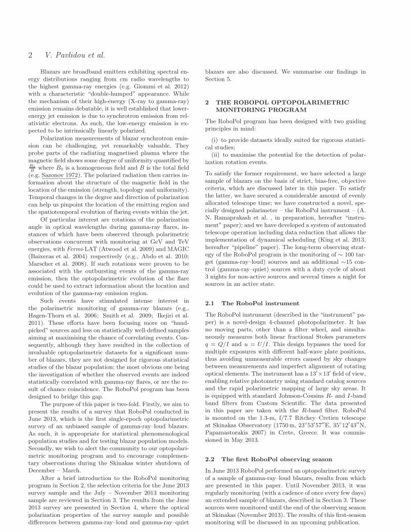
Table 1. Selection criteria for the gamma-ray–loud and the control sample. A summarising chart is shown in Fig. 1.

Property Allowed range for the June survey Allowed range for the 2013 monitoring

Gamma-ray–loud sample

2FGL F (> 100)MeV > 10−8 cm−2 s−1 > 10−8 cm−2 s−1

2FGL source class agu, bzb, or bzq agu, bzb, or bzq

Galactic latitude |b| > 10◦ > 10◦

Elevation (Elv) constrains1 Elv > 30◦ for at least 30min in June Elvmax > 40◦ for at least 120 consecutivedays in the window June – November in-cluding June

R magnitude 6 182 6 17.53

Control sample

CGRaBS/15GHz OVRO monitoring included included

2FGL not included not included

Elevation constrains1 None Elvmax > 40◦ constantly in the windowmid-April – mid-November

R magnitude 6 18 6 17.52

OVRO 15GHz mean flux density N/A > 0.060 Jy

OVRO 15GHz intrinsic modulation in-dex, m

> 0.02 > 0.05

Declination > 54.8◦ (circumpolar) N/A

1Refers to elevation during Skinakas dark hours2Archival value3Average value between archival value and measured during preliminary RoboPol Skinakas observations in June 2012 (when applicable)

2.3 Multi-band monitoring of the RoboPol

sources

All of our sources (including the control sample) are moni-tored twice a week at 15GHz by the OVRO 40-m telescopeblazar monitoring program (Richards et al. 2011). 28 ofthem are also monitored at 30GHz by the Torun 32-m tele-scope (e.g. Browne et al. 2000; Peel et al. 2011). Addition-ally, our sample includes most sources monitored by the F-GAMMA program (Fuhrmann et al. 2007; Angelakis et al.2010) that are visible from Skinakas; for these sources, the F-GAMMA program takes multi-band radio data (total power,linear and circular polarization) approximately once every1.3 months. By design, Fermi-LAT in its sky-scanning modeis continuously providing gamma-ray data for all of ourgamma-ray–loud sources. In this way, our sample has excel-lent multi-band coverage. These multiwavelength data willbe used in the future to correlate the behavior of our sam-ple in optical flux and polarization with the properties andvariations in other wavebands.

3 SAMPLE SELECTION CRITERIA

3.1 Parent Sample

We construct a gamma-ray flux-limited “parent sample” ofgamma-ray–loud blazars from the second Fermi-LAT sourcecatalog (Nolan et al. 2012) using sources tagged as BL Lac

(bzb), FSRQ (bzq), or active galaxy of uncertain type (agu).The parent sample is created the following way:

(i) for each source, we add up Fermi-LAT fluxesabove 100MeV to obtain the integrated photon fluxF (> 100MeV),

(ii) we exclude sources with F (> 100MeV) less than10−8 cm−2 s−1, and

(iii) we exclude sources with galactic latitude |b| < 10◦.

This leaves us with 557 sources in the parent sample. Wehave verified that the sample is truly photon-flux-limitedsince there is no sensitivity dependence on spectral indexor galactic latitude with these cuts. Of these 557 sources,421 are ever observable from Skinakas: they have at leastone night with airmass less than 2, (or, equivalently, eleva-tion higher than 30◦), for at least one hour, within the darkhours of the May – November observing window. Archivaloptical magnitudes were obtained for all 557 sources inthe parent sample mostly in the R-band using the BZ-CAT (Massaro et al. 2009), CGRaBS (Healey et al. 2008b),LQAC 2 (Souchay et al. 2011) and GSC 2.3.2 (Lasker et al.2008) catalogs 1.

1 2 sources were found in V -band, 8 in B-band and 2 in N-band(0.8µm)

4 V. Pavlidou et al.

3.2 June 2013 Survey Sample

The June 2013 survey sample was constructed of parent sam-ple sources with a recorded archival R magnitude less orequal to 18 (R 6 18) which were visible from Skinakas dur-ing dark hours in the month of June 2013 for at least 30minat airmass less than 2. The selection criteria for the candi-date sources in this sample are summarised in Table 1. Thisselection resulted in 142 sources potentially observable inthe month of June which constitute a statistically complete

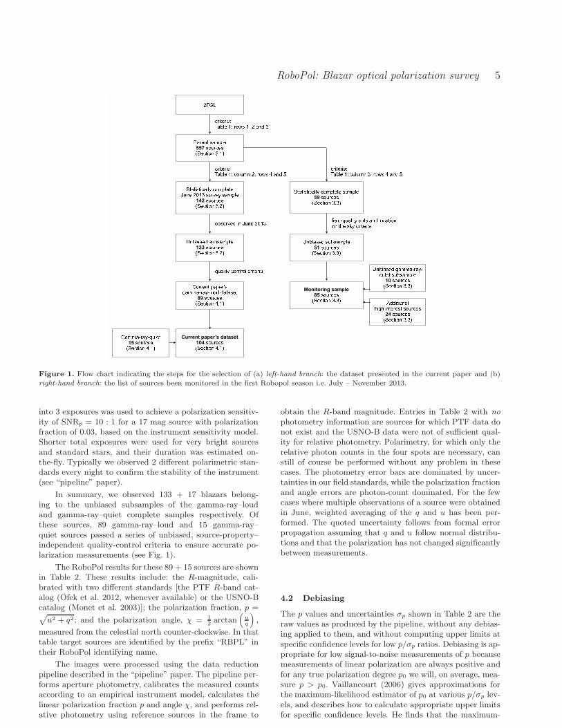
sample. The sources were observed according to a schedul-ing algorithm designed to maximise the number of sourcesthat could be observed in a given time window based on riseand set times, location of sources on the sky, and resultingslewing time of the telescope. At the end of the survey, 133of these sources had been observed. Because the schedulingalgorithm was independent of intrinsic source properties, theresulting set of 133 observed sources is an unbiased subsam-ple of the statistically complete sample of the 142 sources(summary in Fig. 1). The completeness of the sample is 93%for sources brighter than 16 magnitude, 95% (81/85) forsources brighter than 17 magnitude, and 94% (133/142) forsources brighter than 18 magnitude.

To identify sources suitable for inclusion in the “con-trol” sample, a number of non-2FGL CGRaBS (CandidateGamma-Ray Blazar Survey, Healey et al. 2008a) blazarswere also observed during the June survey. Candidatesources for these observations were selected according tothe criteria listed in Table 1. There, the radio variabilityamplitude is quantified through the intrinsic modulation in-

dex m as defined by Richards et al. (2011), which measuresthe flux density standard deviation in units of the meanflux at the source. For the sources discussed in Section 4,m is reported in Table 3. The criteria of Table 1 result in astatistically complete sample of 25 in principle observable,circumpolar, gamma-ray–quiet sources. Of these, 17 sourceswere observed (71%), in order of decreasing polar distance,until the end of our June survey. Since the polar distancecriterion is independent of source properties, the resultinggamma-ray–quiet sources is again an unbiased subsampleof the statistically complete sample of 25 sources. This un-biased subsample is 86% (6/7) complete for sources withR-mag 6 16, 92% (11/12) for sources with R-mag 6 17 andof course 71% (17/24) for sources with R-mag 6 18.

The June 2013 survey results are discussed in Section 4.

3.3 Monitoring Sample

The data collected during the survey phase were used forthe construction of the 2013 observing season monitoringsample which was observed from July 2013 until the endof the 2013 observing season, with an approximate averagecadence of once every 3 days. It consists of three distinctgroups.

(i) An unbiased subsample of a statistically completesample of gamma-ray–loud blazars. Starting from the “par-ent sample” and applying the selection criteria summarisedin Table 1, we obtain a statistically complete sample of 59sources. Application of field-quality cuts (based on data fromthe June survey) and location-on-the-sky criteria that opti-mise continuous observability results in an unbiased subsam-ple of 51 sources.

(ii) An unbiased subsample of a statistically completesample of gamma-ray–quiet blazars. Starting from theCGRaBS, excluding sources in the 2FGL, and applying theselection criteria summarised in Table 1 results in a statis-tically complete sample of 22 sources. Our “control sample”is then an unbiased subsample of 10 blazars, selected fromthis complete sample of gamma-ray–quiet blazars with field-quality and location-on-the-sky criteria.

(iii) 24 additional “high interest” sources, that did nototherwise make it to the sample list.

These observations will later allow the characterisationof each source’s typical behaviour (i.e. average optical fluxand degree of polarization, rate of change of polarization an-gle, flux and polarization degree variability characteristics).This information will be further used to:

(i) improve the optical polarization parameters estimatesfor future polarization population studies,

(ii) develop a dynamical scheduling algorithm, aiming atself-triggering higher cadence observing for blazars display-ing interesting polarization angle rotation events, for the2014 observing season,

(iii) improve the definition of our 2014 monitoring sampleusing a contemporary average, rather than archival single-epoch, optical flux criterion along with some estimate ofthe source variability characteristics in total intensity andin polarized emission.

For the June survey control sample sources, circumpolarsources were selected so that gamma-ray–quiet source obser-vations could be taken at any time and the gamma-ray–loudsources could be prioritized. In contrast, the gamma-ray–quiet sources for the monitoring sample were selected in or-der of increasing declination, to avoid as much as possiblethe northernmost sources which suffer from interference inobservations by strong northern winds at times throughoutthe observing season at Skinakas.

The steps followed for the selection of the June surveysample and the first season monitoring one are summarisedschematically in Fig. 1. The complete sample of our moni-tored sources is available at robopol.org.

4 RESULTS OF JUNE 2013 SURVEY

4.1 Observations

The June survey observations took place between June 1stand June 26th. During that period, we conducted RoboPolobservations, weather permitting, for 21 nights. Of those, 14nights had usable dark hours. The most prohibiting factorshave been wind, humidity and dust, restricting the weatherefficiency to 67%, unusually low based on historical Skinakasweather data. During this period, a substantial amount ofobserving time was spent on system commissioning activi-ties. In the regular monitoring mode of operations a muchhigher efficiency is expected.

During the survey phase a total of 135 gamma-ray–loudtargets (133 of them comprising the unbiased subsampleof the 142-source sample and 2 test targets), 17 potentialcontrol-sample sources, and 10 polarization standards, usedfor calibration purposes, were observed. For the majority ofthe sources, a default exposure time of 15−17.5 min divided

RoboPol: Blazar optical polarization survey 5

Figure 1. Flow chart indicating the steps for the selection of (a) left-hand branch: the dataset presented in the current paper and (b)right-hand branch: the list of sources been monitored in the first Robopol season i.e. July – November 2013.

into 3 exposures was used to achieve a polarization sensitiv-ity of SNRp = 10 : 1 for a 17 mag source with polarizationfraction of 0.03, based on the instrument sensitivity model.Shorter total exposures were used for very bright sourcesand standard stars, and their duration was estimated on-the-fly. Typically we observed 2 different polarimetric stan-dards every night to confirm the stability of the instrument(see “pipeline” paper).

In summary, we observed 133 + 17 blazars belong-ing to the unbiased subsamples of the gamma-ray–loudand gamma-ray–quiet complete samples respectively. Ofthese sources, 89 gamma-ray–loud and 15 gamma-ray–quiet sources passed a series of unbiased, source-property–independent quality-control criteria to ensure accurate po-larization measurements (see Fig. 1).

The RoboPol results for these 89 + 15 sources are shownin Table 2. These results include: the R-magnitude, cali-brated with two different standards [the PTF R-band cat-alog (Ofek et al. 2012, whenever available) or the USNO-Bcatalog (Monet et al. 2003)]; the polarization fraction, p =√

u2 + q2; and the polarization angle, χ = 12arctan

(

uq

)

,

measured from the celestial north counter-clockwise. In thattable target sources are identified by the prefix “RBPL” intheir RoboPol identifying name.

The images were processed using the data reductionpipeline described in the “pipeline” paper. The pipeline per-forms aperture photometry, calibrates the measured countsaccording to an empirical instrument model, calculates thelinear polarization fraction p and angle χ, and performs rel-ative photometry using reference sources in the frame to

obtain the R-band magnitude. Entries in Table 2 with no

photometry information are sources for which PTF data donot exist and the USNO-B data were not of sufficient qual-ity for relative photometry. Polarimetry, for which only therelative photon counts in the four spots are necessary, canstill of course be performed without any problem in thesecases. The photometry error bars are dominated by uncer-tainties in our field standards, while the polarization fractionand angle errors are photon-count dominated. For the fewcases where multiple observations of a source were obtainedin June, weighted averaging of the q and u has been per-formed. The quoted uncertainty follows from formal errorpropagation assuming that q and u follow normal distribu-tions and that the polarization has not changed significantlybetween measurements.

4.2 Debiasing

The p values and uncertainties σp shown in Table 2 are theraw values as produced by the pipeline, without any debias-ing applied to them, and without computing upper limits atspecific confidence levels for low p/σp ratios. Debiasing is ap-propriate for low signal-to-noise measurements of p becausemeasurements of linear polarization are always positive andfor any true polarization degree p0 we will, on average, mea-sure p > p0. Vaillancourt (2006) gives approximations forthe maximum-likelihood estimator of p0 at various p/σp lev-els, and describes how to calculate appropriate upper limitsfor specific confidence levels. He finds that the maximum-

6 V. Pavlidou et al.

0 0.05 0.1 0.15 0.2 0.25polarization fraction

0

0.2

0.4

0.6

0.8

1

cum

ulat

ive

dist

ribu

tion

func

tion

gamma-ray loudgamma-ray quiet

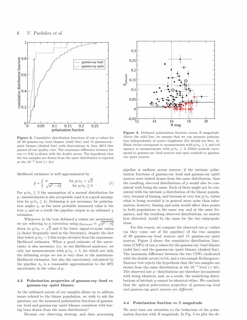
Figure 2. Cumulative distribution functions of raw p values forall 89 gamma-ray–loud blazars (solid line) and 15 gamma-ray–quiet blazars (dashed line) with observations in June 2013 thatpassed all our quality cuts. The maximum difference between thetwo (= 0.6) is shown with the double arrow. The hypothesis thatthe two samples are drawn from the same distribution is rejected

at the 10−3 level (> 3σ).

likelihood estimator is well approximated by

p =

{

0 for p/σp <√2

√

p2 − σ2p for p/σp & 3

. (1)

For p/σp & 3 the assumption of a normal distribution forp−measurements is also acceptable (and it is a good assump-tion for p/σp & 4). Debiasing is not necessary for polariza-tion angles χ, as the most probable measured value is thetrue χ and as a result the pipeline output is an unbiased χestimator.

Whenever in the text debiased p values are mentioned,we are referring to a correction using pdebiased ≈

√

p2 − σ2p

down to p/σp =√2 and 0 for lower signal-to-noise ratios

(a choice frequently used in the literature), despite the factthat below p/σp ∼ 3 this recipe deviates from the maximum-likelihood estimator. When a good estimate of the uncer-tainty is also necessary (i.e. in our likelihood analyses), weonly use measurements with p/σp > 3, for which not onlythe debiasing recipe we use is very close to the maximum-likelihood estimator, but also the uncertainty calculated bythe pipeline σp is a reasonable approximation to the 68%uncertainty in the value of p.

4.3 Polarization properties of gamma-ray–loud vs

gamma-ray–quiet blazars

As the unbiased nature of our samples allows us to addressissues related to the blazar population, we wish to ask thequestion: are the measured polarization fractions of gamma-ray–loud and gamma-ray–quiet blazars consistent with hav-ing been drawn from the same distribution?

Because our observing strategy and data processing

12 14 16 18 20R mag

-0.05

0

0.05

0.1

0.15

0.2

0.25

0.3

p debi

ased

Figure 3. Debiased polarization fraction versus R magnitude.Above the solid line, we assume that we can measure polariza-tion independently of source brightness (for details see Sect. 4).Black circles correspond to measurements with p/σp > 3, and redsquares to measurements with p/σp < 3. Filled symbols corre-spond to gamma-ray–loud sources and open symbols to gamma-ray–quiet sources.

pipeline is uniform across sources, if the intrinsic polar-ization fractions of gamma-ray–loud and gamma-ray–quietsources were indeed drawn from the same distribution, thenthe resulting observed distributions of p would also be con-sistent with being the same. Each of them might not be con-sistent with the intrinsic p distribution of the blazar popula-tion, because of biasing, and because at very low p/σp valueswhat is being recorded is in general more noise than infor-mation; however, biasing and noise would affect data pointsin both populations in the same way and at the same fre-quency, and the resulting observed distributions, no matterhow distorted, would be the same for the two subpopula-tions.

For this reason, we compare the observed raw p−values(as they come out of the pipeline) of the two samplesof 89 gamma-ray–loud sources and 15 gamma-ray–quietsources. Figure 2 shows the cumulative distribution func-tions (CDFs) of raw p values for the gamma-ray–loud blazars(solid line) and the gamma-ray–quiet blazars (dashed line).The maximum difference between the two CDFs (indicatedwith the double arrow) is 0.6, and a two-sample Kolmogorov-Smirnov test rejects the hypothesis that the two samples aredrawn from the same distribution at the 10−3 level (> 3σ).The observed raw p−distributions are therefore inconsistentwith being identical, and, as a result, the underlying distri-butions of intrinsic p cannot be identical either. We concludethat the optical polarization properties of gamma-ray–loud

and gamma-ray–quiet sources are different.

4.4 Polarization fraction vs R magnitude

We next turn our attention to the behaviour of the polar-ization fraction with R magnitude. In Fig. 3 we plot the de-

RoboPol: Blazar optical polarization survey 7

biased value of the polarization fraction as a function of themeasured R magnitude for each source. Sources for whichp/σp < 3 are shown with red colour. There are two notewor-thy pictures in this plot: the clustering of low signal-to-noiseratio measurements in the lower-right corner of the plot, andthe scarcity of observations in the upper-left part of the plot.

The first effect is expected, as low polarization fractionsare harder to measure for fainter sources with fixed time in-tegration. This is a characteristic of the June survey ratherthan the RoboPol program in general: in monitoring mode,RoboPol scheduling features adaptive integration time toachieve a uniform signal-to-noise ratio down to a fixed polar-ization value for any source brightness. For source brightnesshigher than magnitude of 17 we have measured polarizationfractions down to 1.5 × 10−2: most measurements at thatlevel have p/σp > 3. For source brightness lower than mag-nitude of 18 the same is true for polarization fractions downto 3.5 × 10−2. These limits are shown with the thick solidline in Fig. 3, and they are further discussed in Section 4.5in the context of our likelihood analysis to determine themost likely intrinsic distributions of polarization fractionsfor gamma-ray–loud and gamma-ray–quiet sources.

The second effect – the lack of data points for R magni-tudes lower than 16 and polarization fractions higher than1.25× 10−2 as indicated by the dotted lines – may be astro-physical in origin: in sources where unpolarized light fromthe host galaxy is a significant contribution to the overallflux, the polarization fraction should be on average lower.This contribution also tends to make these sources on av-erage brighter. We will return to a quantitative evaluationand analysis of this effect when we present data from ourfirst season of monitoring, using both data from the litera-ture as well as our own variability information to constrainthe possible contribution from the host for as many of oursources as possible.

4.5 Intrinsic distributions of polarization fraction

In Section 4.3 we showed that the intrinsic distributions ofpolarization fraction of gamma-ray–quiet and gamma-ray–loud blazars must be different; however, that analysis did notspecify what these individual intrinsic distributions mightbe. We address this issue in this section. Our approach con-sists of two steps. First, we will determine what the overallshape of the distributions looks like, and we will thus selecta family of probability distribution functions that can bestdescribe the intrinsic probability distribution of polarizationfraction in blazars. Next, we will use a likelihood analysis toproduce best-guess estimates and confidence limits on theparameters of these distributions for each subpopulation.

4.5.1 Selection of Family of Distributions

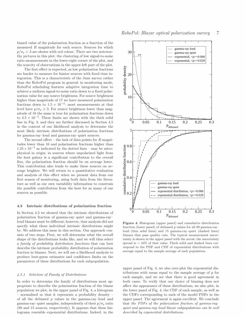
In order to determine the family of distributions most ap-propriate to describe the polarization fraction of the blazarpopulation we plot, in the upper panel of Fig. 4, a histogram– normalised so that it represents a probability density –of all the debiased p values in the gamma-ray–loud andgamma-ray–quiet samples, independently of their p/σp ratio(89 and 15 sources, respectively). It appears that these his-tograms resemble exponential distributions. Indeed, in the

0 0.05 0.1 0.15 0.2 0.25 0.3p

debiased

0

10

20

30

prob

abili

ty d

ensi

ty

gamma-ray loud gamma-ray quietexponential, <p>=0.066exponential, <p>=0.029

0 0.05 0.1 0.15 0.2 0.25 0.3p

debiased

0

0.2

0.4

0.6

0.8

1

cum

ulat

ive

dist

ribu

tion

func

tion

gamma-ray loudgamma-ray quietexponential distribution, <p>=0.066exponential distribution, <p>=0.029

Figure 4. Histogram (upper panel) and cumulative distributionfunction (lower panel) of debiased p values for all 89 gamma-ray–loud (thin solid lines) and 15 gamma-ray–quiet (dashed lines)blazars that pass quality cuts. The typical measurement uncer-tainty is shown in the upper panel with the arrow; the uncertaintyspread is ∼ 10% of that value. Thick solid and dashed lines cor-respond to the PDF and CDF of exponential distributions withaverage equal to the sample average of each population.

upper panel of Fig. 4, we also over-plot the exponential dis-tributions with mean equal to the sample average of p foreach sample, and we see that there is good agreement inboth cases. To verify that our choice of binning does notaffect the appearance of these distributions, we also plot, inthe lower panel of Fig. 4, the CDF of each sample, as well asthe CDFs corresponding to each of the model PDFs in theupper panel. The agreement is again excellent. We concludethat the PDFs of the polarization fraction of gamma-ray–

quiet and gamma-ray–loud blazar subpopulations can be well

described by exponential distributions.

8 V. Pavlidou et al.

0 0.1 0.2<p>

0

10

20

30

40

50

likel

ihoo

d

gamma-ray loudgamma-ray quiet

-0.2 -0.1 0 0.1 0.2<p>

quiet - <p>

loud

0

5

10

15

20

25

30

likel

ihoo

d

1σ

2σ

most probable

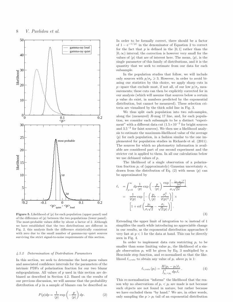
Figure 5. Likelihood of 〈p〉 for each population (upper panel) andof the difference of 〈p〉 between the two populations (lower panel).The most-probable values differ by about a factor of 2. Althoughwe have established that the two distributions are different inFig. 2, this analysis finds the difference statistically consistentwith zero due to the small number of gamma-ray–quiet sourcessurviving the strict signal-to-noise requirements of this section.

4.5.2 Determination of Distribution Parameters

In this section, we seek to determine the best-guess valuesand associated confidence intervals for the parameters of theintrinsic PDFs of polarization fraction for our two blazarsubpopulations. All values of p used in this section are de-biased as described in Section 4.2. Based on the results ofour previous discussion, we will assume that the probabilitydistribution of p in a sample of blazars can be described as

P (p)dp =1

〈p〉 exp(

− p

〈p〉

)

dp . (2)

In order to be formally correct, there should be a factorof 1 − e−1/〈p〉 in the denominator of Equation 2 to correctfor the fact that p is defined in the [0, 1] rather than the[0,∞) interval; the correction is however very small for thevalues of 〈p〉 that are of interest here. The mean, 〈p〉, is thesingle parameter of this family of distributions, and it is thequantity that we seek to estimate from our data for eachsubsample.

In the population studies that follow, we will includeonly sources with p/σp > 3. However, in order to avoid bi-asing our statistics by this choice, we apply sharp cuts inp−space that exclude most, if not all, of our low p/σp mea-surements; these cuts can then be explicitly corrected for inour analysis (which will assume that sources below a certainp value do exist, in numbers predicted by the exponentialdistribution, but cannot be measured). These selection cri-teria are visualised by the thick solid line in Fig. 3.

We thus split each population into two sub-samples,along the (measured) R-mag 17 line, and, for each popula-tion, we consider each subsample to be a distinct “experi-ment” with a different data cut (1.5×10−2 for bright sourcesand 3.5−2 for faint sources). We then use a likelihood analy-sis to estimate the maximum-likelihood value of the average〈p〉 for each population, in a fashion similar to the one im-plemented for population studies in Richards et al. (2011).The sources for which no photometry information is avail-able are considered part of our second experiment and thestricter cut is applied to them. In all our calculations belowwe use debiased values of p.

The likelihood of a single observation of a polariza-tion fraction pi of (approximately) Gaussian uncertainty σi

drawn from the distribution of Eq. (2) with mean 〈p〉 canbe approximated by

ℓi =

∫ ∞

p=0

dp1

〈p〉 exp(

− p

〈p〉

) exp[

− (p−pi)2

2σ2

i

]

σi

√2π

=1

2〈p〉 exp[

−(

pi〈p〉 −

σ2i

2〈p〉2)]

×[

1 + erf

(

pi

σi

√2− σi√

2〈p〉

)]

.

(3)

Extending the upper limit of integration to ∞ instead of 1simplifies the math while introducing no appreciable changein our results, as the exponential distribution approaches 0very fast at p < 1 for the data at hand. This can be directlyseen in Fig. 4.

In order to implement data cuts restricting pi to besmaller than some limiting value pl, the likelihood of a sin-gle observation pi will be given by Eq. 3 multiplied by aHeaviside step function, and re-normalised so that the like-lihood ℓi,cuts to obtain any value of pi above pl is 1:

ℓi,cuts (pl) =H(pi − pl)ℓi∫ 1

pi=pldpiℓi

. (4)

This re-normalisation “informs” the likelihood that the rea-son why no observations of pi < pl are made is not becausesuch objects are not found in nature, but rather becausewe have excluded them “by hand.” We are, in other words,only sampling the p > pl tail of an exponential distribution

RoboPol: Blazar optical polarization survey 9

of mean 〈p〉. The likelihood of N observations of this type is

L(〈p〉) =N∏

i=1

ℓi,cuts (pl) , (5)

and the combination of two experiments with distinct datacuts, described above, will have a likelihood equal to

L(〈p〉) =Nl∏

i=1

ℓi,cuts (pl)

Nu∏

j=1

ℓj,cuts (pu) , (6)

where Nl (equal to 41 for the gamma-ray–loud sources and 7for the gamma-ray–quiet sources) is the number of p/σp > 3objects with R-mag < 17 surviving the pl = 0.015 cut, andNu (equal to 20 for the gamma-ray–loud sources and 1 forthe gamma-ray–quiet sources) is the number of p/σp > 3 ob-jects with R-mag > 17 or no photometry information sur-viving the pu = 0.035 cut. Maximising Eq. (6) we obtainthe maximum-likelihood value of 〈p〉. Statistical uncertain-ties on this value can also be obtained in a straight-forwardway, as Eq. (6), assuming a flat prior on 〈p〉, gives the prob-ability density of the mean polarization fraction 〈p〉 of thepopulation under study.

The upper panel of Fig. 5 shows the likelihood of 〈p〉for the gamma-ray–loud (solid line) and gamma-ray–quiet(dashed line) populations. The maximum-likelihood esti-mate of 〈p〉 with its 68% confidence intervals is 6.7+1.0

−0.8×10−2

for gamma-ray–loud blazars and 3.2+1.8−1.0 × 10−2 for gamma-

ray–quiet blazars. The maximum-likelihood values of 〈p〉 dif-fer by more than a factor of 2, consistent with our earlierfinding that the two populations have different polarizationfraction PDFs. However, because of the small number ofgamma-ray–quiet sources surviving the strict signal-to-noisecuts we have imposed in this section (only 8 objects), thegamma-ray–quiet 〈p〉 cannot be pinpointed with enough ac-curacy and its corresponding likelihood exhibits a long tailtowards high values. For this reason, the probability distri-bution of the difference between the 〈p〉 of the two popula-tions, which is quantified by the cross-correlation of the twolikelihoods, has a peak, at a difference of 3.4 × 10−2, whichis less than 2σ from zero. This result is shown in the lowerpanel of Fig. 5.

The accuracy with which the gamma-ray–quiet 〈p〉 isestimated can be improved in two ways. First, by an im-proved likelihood analysis which allows us to properly treateven low p/σp sources. And second, by an improved sur-vey of the gamma-ray–quiet population (more sources toimprove sample statistics, and longer exposures to improvethe accuracy of individual p measurements).

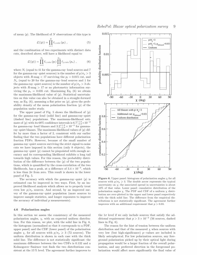
4.6 Polarization angles

In this section we assess the consistency of the measuredpolarization angles, χ, with an expected uniform distribu-tion. For this reason, we plot, with the solid line in Fig. 6,the histogram (normalised so that it corresponds to a PDF,upper panel) and the CDF (lower panel) of the polarizationangles χ, for all sources with p/σp > 3 (72 sources). Theuniform distribution is shown in each case with the thicksolid line. The difference is not statistically significant: themaximum difference between the two CDFs is 0.132 and aKolmogorov–Smirnov test finds the two distributions con-sistent at the 15% level. The agreement further improves to

-90 -60 -30 0 30 60 90χ (deg)

0

0.005

0.01

0.015

prob

abili

ty d

istr

ibut

ion

func

tion

p/σp>3

p/σp>3, p

debiased>0.03

Uniform

-90 -60 -30 0 30 60 90 χ (deg)

0

0.2

0.4

0.6

0.8

1cu

mul

ativ

e di

stri

butio

n fu

nctio

n

All blazars with p/ σp>3

Additional cut: pdebiased

>0.03

Uniform distribution

Figure 6. Upper panel: histogram of polarization angles χ for allsources with p/σp > 3. The double arrow represents the typicaluncertainty on χ; the associated spread in uncertainties is about10% of that value. Lower panel: cumulative distribution of thepolarization angles χ. The PDF and CDF of a uniform χ distri-bution are over-plotted in the upper and lower panel respectivelywith the thick solid line. The difference from the empirical dis-tributions is not statistically significant. The agreement furtherimproves with an additional requirement that p > 0.03.

the 1σ level if we only include sources that satisfy the ad-ditional requirement that p > 3× 10−2 (56 sources, dashedlines in Fig. 6).

The reason for the hint of tension between the uniformdistribution and that of the measured χ when sources withvery low (but high-significance) p−values are included islikely astrophysical. For low polarization sources, any fore-ground polarization picked up by their optical light duringpropagation would be a larger fraction of the overall polar-ization, and any preferred direction in the foreground po-larization would affect more significantly the final value of

10 V. Pavlidou et al.

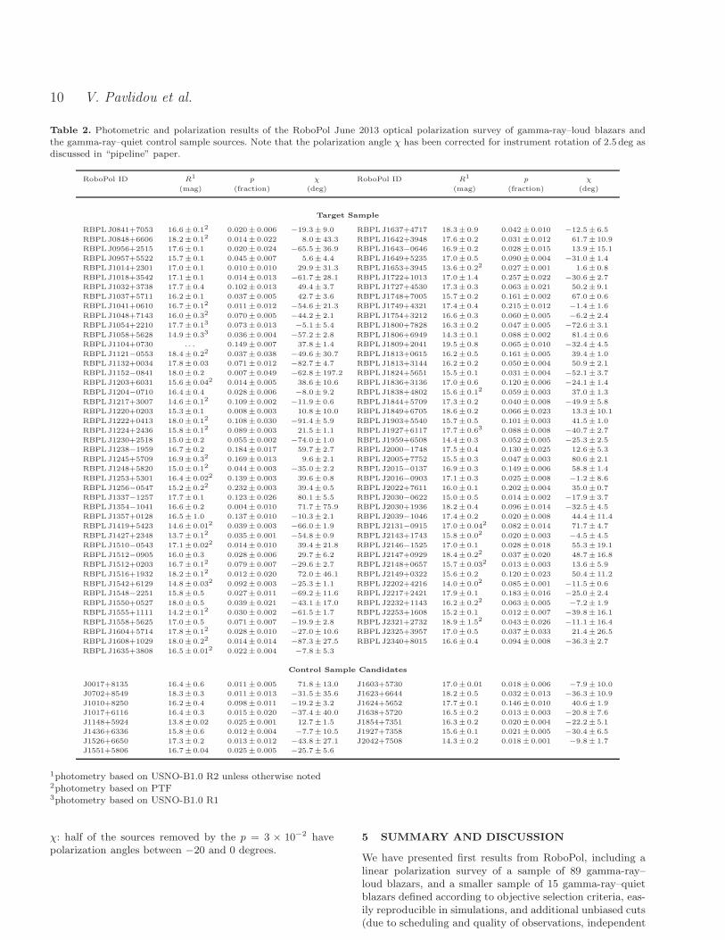
Table 2. Photometric and polarization results of the RoboPol June 2013 optical polarization survey of gamma-ray–loud blazars andthe gamma-ray–quiet control sample sources. Note that the polarization angle χ has been corrected for instrument rotation of 2.5 deg asdiscussed in “pipeline” paper.

RoboPol ID R1 p χ RoboPol ID R1 p χ

(mag) (fraction) (deg) (mag) (fraction) (deg)

Target Sample

RBPLJ0841+7053 16.6± 0.12 0.020± 0.006 −19.3± 9.0 RBPL J1637+4717 18.3± 0.9 0.042± 0.010 −12.5± 6.5

RBPLJ0848+6606 18.2± 0.12 0.014± 0.022 8.0± 43.3 RBPL J1642+3948 17.6± 0.2 0.031± 0.012 61.7± 10.9

RBPLJ0956+2515 17.6± 0.1 0.020± 0.024 −65.5± 36.9 RBPL J1643−0646 16.9± 0.2 0.028± 0.015 13.9± 15.1

RBPLJ0957+5522 15.7± 0.1 0.045± 0.007 5.6± 4.4 RBPL J1649+5235 17.0± 0.5 0.090± 0.004 −31.0± 1.4

RBPLJ1014+2301 17.0± 0.1 0.010± 0.010 29.9± 31.3 RBPL J1653+3945 13.6± 0.22 0.027± 0.001 1.6± 0.8

RBPLJ1018+3542 17.1± 0.1 0.014± 0.013 −61.7± 28.1 RBPL J1722+1013 17.0± 1.4 0.257± 0.022 −30.6± 2.7

RBPLJ1032+3738 17.7± 0.4 0.102± 0.013 49.4± 3.7 RBPL J1727+4530 17.3± 0.3 0.063± 0.021 50.2± 9.1

RBPLJ1037+5711 16.2± 0.1 0.037± 0.005 42.7± 3.6 RBPL J1748+7005 15.7± 0.2 0.161± 0.002 67.0± 0.6

RBPLJ1041+0610 16.7± 0.12 0.011± 0.012 −54.6± 21.3 RBPL J1749+4321 17.4± 0.4 0.215± 0.012 −1.4± 1.6

RBPLJ1048+7143 16.0± 0.32 0.070± 0.005 −44.2± 2.1 RBPL J1754+3212 16.6± 0.3 0.060± 0.005 −6.2± 2.4

RBPLJ1054+2210 17.7± 0.13 0.073± 0.013 −5.1± 5.4 RBPL J1800+7828 16.3± 0.2 0.047± 0.005 −72.6± 3.1

RBPLJ1058+5628 14.9± 0.33 0.036± 0.004 −57.2± 2.8 RBPL J1806+6949 14.3± 0.1 0.088± 0.002 81.4± 0.6

RBPLJ1104+0730 . . . 0.149± 0.007 37.8± 1.4 RBPL J1809+2041 19.5± 0.8 0.065± 0.010 −32.4± 4.5

RBPLJ1121−0553 18.4± 0.22 0.037± 0.038 −49.6± 30.7 RBPL J1813+0615 16.2± 0.5 0.161± 0.005 39.4± 1.0

RBPLJ1132+0034 17.8± 0.03 0.071± 0.012 −82.7± 4.7 RBPL J1813+3144 16.2± 0.2 0.050± 0.004 50.9± 2.1

RBPLJ1152−0841 18.0± 0.2 0.007± 0.049 −62.8± 197.2 RBPL J1824+5651 15.5± 0.1 0.031± 0.004 −52.1± 3.7

RBPLJ1203+6031 15.6± 0.042 0.014± 0.005 38.6± 10.6 RBPL J1836+3136 17.0± 0.6 0.120± 0.006 −24.1± 1.4

RBPLJ1204−0710 16.4± 0.4 0.028± 0.006 −8.0± 9.2 RBPL J1838+4802 15.6± 0.12 0.059± 0.003 37.0± 1.3

RBPLJ1217+3007 14.6± 0.12 0.109± 0.002 −11.9± 0.6 RBPL J1844+5709 17.3± 0.2 0.040± 0.008 −49.9± 5.8

RBPLJ1220+0203 15.3± 0.1 0.008± 0.003 10.8± 10.0 RBPL J1849+6705 18.6± 0.2 0.066± 0.023 13.3± 10.1

RBPLJ1222+0413 18.0± 0.12 0.108± 0.030 −91.4± 5.9 RBPL J1903+5540 15.7± 0.5 0.101± 0.003 41.5± 1.0

RBPLJ1224+2436 15.8± 0.12 0.089± 0.003 21.5± 1.1 RBPL J1927+6117 17.7± 0.63 0.088± 0.008 −40.7± 2.7

RBPLJ1230+2518 15.0± 0.2 0.055± 0.002 −74.0± 1.0 RBPL J1959+6508 14.4± 0.3 0.052± 0.005 −25.3± 2.5

RBPLJ1238−1959 16.7± 0.2 0.184± 0.017 59.7± 2.7 RBPL J2000−1748 17.5± 0.4 0.130± 0.025 12.6± 5.3

RBPLJ1245+5709 16.9± 0.32 0.169± 0.013 9.6± 2.1 RBPL J2005+7752 15.5± 0.3 0.047± 0.003 80.6± 2.1

RBPLJ1248+5820 15.0± 0.12 0.044± 0.003 −35.0± 2.2 RBPL J2015−0137 16.9± 0.3 0.149± 0.006 58.8± 1.4

RBPLJ1253+5301 16.4± 0.022 0.139± 0.003 39.6± 0.8 RBPL J2016−0903 17.1± 0.3 0.025± 0.008 −1.2± 8.6

RBPLJ1256−0547 15.2± 0.22 0.232± 0.003 39.4± 0.5 RBPL J2022+7611 16.0± 0.1 0.202± 0.004 35.0± 0.7

RBPLJ1337−1257 17.7± 0.1 0.123± 0.026 80.1± 5.5 RBPL J2030−0622 15.0± 0.5 0.014± 0.002 −17.9± 3.7

RBPLJ1354−1041 16.6± 0.2 0.004± 0.010 71.7± 75.9 RBPL J2030+1936 18.2± 0.4 0.096± 0.014 −32.5± 4.5

RBPLJ1357+0128 16.5± 1.0 0.137± 0.010 −10.3± 2.1 RBPL J2039−1046 17.4± 0.2 0.020± 0.008 44.4± 11.4

RBPLJ1419+5423 14.6± 0.012 0.039± 0.003 −66.0± 1.9 RBPL J2131−0915 17.0± 0.042 0.082± 0.014 71.7± 4.7

RBPLJ1427+2348 13.7± 0.12 0.035± 0.001 −54.8± 0.9 RBPL J2143+1743 15.8± 0.02 0.020± 0.003 −4.5± 4.5

RBPLJ1510−0543 17.1± 0.022 0.014± 0.010 39.4± 21.8 RBPL J2146−1525 17.0± 0.1 0.028± 0.018 55.3± 19.1

RBPLJ1512−0905 16.0± 0.3 0.028± 0.006 29.7± 6.2 RBPL J2147+0929 18.4± 0.22 0.037± 0.020 48.7± 16.8

RBPLJ1512+0203 16.7± 0.12 0.079± 0.007 −29.6± 2.7 RBPL J2148+0657 15.7± 0.032 0.013± 0.003 13.6± 5.9

RBPLJ1516+1932 18.2± 0.12 0.012± 0.020 72.0± 46.1 RBPL J2149+0322 15.6± 0.2 0.120± 0.023 50.4± 11.2

RBPLJ1542+6129 14.8± 0.032 0.092± 0.003 −25.3± 1.1 RBPL J2202+4216 14.0± 0.02 0.085± 0.001 −11.5± 0.6

RBPLJ1548−2251 15.8± 0.5 0.027± 0.011 −69.2± 11.6 RBPL J2217+2421 17.9± 0.1 0.183± 0.016 −25.0± 2.4

RBPLJ1550+0527 18.0± 0.5 0.039± 0.021 −43.1± 17.0 RBPL J2232+1143 16.2± 0.22 0.063± 0.005 −7.2± 1.9

RBPLJ1555+1111 14.2± 0.12 0.030± 0.002 −61.5± 1.7 RBPL J2253+1608 15.2± 0.1 0.012± 0.007 −39.8± 16.1

RBPLJ1558+5625 17.0± 0.5 0.071± 0.007 −19.9± 2.8 RBPL J2321+2732 18.9± 1.52 0.043± 0.026 −11.1± 16.4

RBPLJ1604+5714 17.8± 0.12 0.028± 0.010 −27.0± 10.6 RBPL J2325+3957 17.0± 0.5 0.037± 0.033 21.4± 26.5

RBPLJ1608+1029 18.0± 0.22 0.014± 0.014 −87.3± 27.5 RBPL J2340+8015 16.6± 0.4 0.094± 0.008 −36.3± 2.7

RBPLJ1635+3808 16.5± 0.012 0.022± 0.004 −7.8± 5.3

Control Sample Candidates

J0017+8135 16.4± 0.6 0.011± 0.005 71.8± 13.0 J1603+5730 17.0± 0.01 0.018± 0.006 −7.9± 10.0

J0702+8549 18.3± 0.3 0.011± 0.013 −31.5± 35.6 J1623+6644 18.2± 0.5 0.032± 0.013 −36.3± 10.9

J1010+8250 16.2± 0.4 0.098± 0.011 −19.2± 3.2 J1624+5652 17.7± 0.1 0.146± 0.010 40.6± 1.9

J1017+6116 16.4± 0.3 0.015± 0.020 −37.4± 40.0 J1638+5720 16.5± 0.2 0.013± 0.003 −20.8± 7.6

J1148+5924 13.8± 0.02 0.025± 0.001 12.7± 1.5 J1854+7351 16.3± 0.2 0.020± 0.004 −22.2± 5.1

J1436+6336 15.8± 0.6 0.012± 0.004 −7.7± 10.5 J1927+7358 15.6± 0.1 0.021± 0.005 −30.4± 6.5

J1526+6650 17.3± 0.2 0.013± 0.012 −43.8± 27.1 J2042+7508 14.3± 0.2 0.018± 0.001 −9.8± 1.7

J1551+5806 16.7± 0.04 0.025± 0.005 −25.7± 5.6

1photometry based on USNO-B1.0 R2 unless otherwise noted2photometry based on PTF3photometry based on USNO-B1.0 R1

χ: half of the sources removed by the p = 3 × 10−2 havepolarization angles between −20 and 0 degrees.

5 SUMMARY AND DISCUSSION

We have presented first results from RoboPol, including alinear polarization survey of a sample of 89 gamma-ray–loud blazars, and a smaller sample of 15 gamma-ray–quietblazars defined according to objective selection criteria, eas-ily reproducible in simulations, and additional unbiased cuts(due to scheduling and quality of observations, independent

RoboPol: Blazar optical polarization survey 11

of source properties). These results are therefore represen-tative of the gamma-ray–loud and gamma-ray–quiet blazarpopulations, and as such are appropriate for populationsstudies.

Our findings can be summarised as follows:

• The hypothesis that the polarization fractions ofgamma-ray–loud and gamma-ray quiet blazars are drawnfrom the same distribution is rejected at the 10−3 level.

• The probability distribution functions of polarizationfraction of gamma-ray–loud and gamma-ray–quiet blazarscan be well described by exponential distributions.

• Using a likelihood analysis we estimate the best-guessvalues and 1σ uncertainties of the mean polarization fractionof each subpopulation, which is the single parameter charac-terising an exponential distribution. We find 〈p〉 = 6.7+1.0

−0.8×10−2 for gamma-ray–loud blazars, and 〈p〉 = 3.2+1.8

−1.0 × 10−2

for gamma-ray–quiet blazars.• The large upwards uncertainty of 〈p〉 for gamma-ray–

quiet blazars is a side-effect of the strict cuts we have appliedin our likelihood analysis, leaving us only with 8 useablesources for the gamma-ray–quiet sample. This is the reasonwhy the statistical inconsistency between the two popula-tions cannot be also verified with this method. This prob-lem can be improved with a larger gamma-ray–quiet blazarsurvey, longer integration times, and a more sophisticatedanalysis.

• Polarization angles, χ, for blazars in our survey are con-sistent with being drawn from a uniform distribution.

It is the first time a statistical difference between theaverage polarization properties of gamma-ray–quiet andgamma-ray–loud blazars is demonstrated in optical wave-lengths. The difference is consistent with the findings ofHovatta et al. (2010) for the radio polarization of gamma-ray–loud and, otherwise similar, gamma-ray–quiet sources.It thus appears that the gamma-ray–loud blazars overall ex-hibit higher degree of polarization in their synchrotron emis-sion than their gamma-ray–quiet counterparts. As we havediscussed in Section 1, the degree of polarization is a mea-sure of the degree of uniformity of the magnetic field overthe emission region. The bulk of synchrotron in gamma-ray–loud blazars seems therefore to originate in regions ofhigher magnetic field uniformity than the emission fromgamma-ray–quiet blazars. It is possible that shocks that arestrong/persistent enough to accelerate particles capable ofgamma-ray emission are also better in locally aligning mag-netic field lines and producing regions of high field unifor-mity, hence a higher polarization degree.

We have found hints of depolarization at high opticalfluxes, an effect that may be attributable to the contribu-tion of unpolarized light to the overall flux by the blazar’shost galaxy. The statistics of BL Lac hosts at least are con-sistent with this idea: in about 50% of the sources studiedby Nilsson et al. (2003) the host would have a contributionof more than 50% the core flux inside our typical aperture.We will examine the effect quantitatively and in more detailusing our full first season data in an upcoming publication.

Inclusion of sources of very low (but significantly mea-sured) polarization fraction in the empirical distribution ofpolarization angles generates some tension (although stillnot statistically significant) between that distribution andan expected uniform one. This may be a result of foreground

polarization at a preferred direction, which, although smalland not important for high-polarization sources, tends toalign lower polarization sources. Although the sources inthe RoboPol sample have been selected to lie away fromthe Galactic plane so foreground polarization due to inter-stellar dust absorption should be at a minimum, nearby in-terstellar material might also induce some degree of fore-ground polarization. For example, such an effect, at thep ∼ 0.8 × 10−2 level, has been seen in the southern sky bySantos et al. (2013). A similar level of foreground polariza-tion, p ∼ 0.9× 10−2, has been suggested by Sillanpaa et al.(1993) for the vicinity of BL Lac (which however lies at rela-tively low Galactic latitude b ∼ −10◦). A cut at p > 3×10−2

ensures that sources are intrinsically at least twice as po-larized as that, so the effect in measured χ is minimised.Because the 13′ × 13′ fields around sources in our monitor-ing program accumulate exposure during our observing sea-son, we will be eventually able to measure the polarizationproperties of non-variable, intrinsically unpolarized sourcesinduced by foregrounds to higher accuracy, and better studyand correct for this effect in the future.

For the remainder of the 2013 season we have beenmonitoring a 3-element sample in linear polarization withRoboPol: an unbiased gamma-ray–loud blazar sample (51sources); a smaller, again unbiased, gamma-ray–quiet sam-ple (10 sources); and a list of high-interest sources that havenot made our cuts (24 sources). After the end of the 2013season, we will present first light curves and analysis ofour sources in terms of polarization variability and cross-correlations in the amplitude and time domains. Finally, wewill revisit our monitoring sample definition, to strengthenthe robustness of criteria (for example, using RoboPol aver-age R-band fluxes for the R-magnitude cuts), and to de-velop our automatic scheduling algorithm which aims toself-trigger high cadence observations during polarizationchanges that are unusually fast for a specific source. In thisway, we aim to better constrain the linear polarization prop-erties of the blazar population at optical wavelengths andto provide a definitive answer to whether a significant frac-tion of fast polarization rotations do indeed coincide withgamma-ray flares.

ACKNOWLEDGMENTS

The U. of Crete group is acknowledging support by the“RoboPol” project, which is implemented under the “ARIS-TEIA” Action of the “OPERATIONAL PROGRAMMEEDUCATION AND LIFELONG LEARNING” and is co-funded by the European Social Fund (ESF) and Greek Na-tional Resources. The NCU group is acknowledging sup-port from the Polish National Science Centre (PNSC), grantnumber 2011/01/B/ST9/04618. This research is supportedin part by NASA grants NNX11A043G and NSF grant AST-1109911. V.P. is acknowledging support by the EuropeanCommission Seventh Framework Programme (FP7) throughthe Marie Curie Career Integration Grant PCIG10-GA-2011-304001 “JetPop”. K.T. is acknowledging support byFP7 through Marie Curie Career Integration Grant PCIG-GA-2011-293531 “SFOnset”. V.P., E.A., I.M., K.T., andJ.A.Z. would like to acknowledge partial support from theEU FP7 Grant PIRSES-GA-2012-31578 “EuroCal”. I.M. is

12 V. Pavlidou et al.

supported for this research through a stipend from the In-ternational Max Planck Research School (IMPRS) for As-tronomy and Astrophysics at the Universities of Bonn andCologne. M.B. acknowledges support from the InternationalFulbright Science and Technology Award. T.H. was sup-ported in part by the Academy of Finland project num-ber 267324. The RoboPol collaboration acknowledges ob-servations support from the Skinakas Observatory, operatedjointly by the U. of Crete and the Foundation for Researchand Technology - Hellas. Support from MPIfR, PNSC, theCaltech Optical Observatories, and IUCAA for the designand construction of the RoboPol polarimeter is also acknowl-edged. Finally, V.P. and E.A. thank the internal referee atthe MPIfR Dr. F. Mantovani for the useful comments on thefinal manuscript.

REFERENCES

Abdo A. A., Ackermann M., Ajello M., et al., 2010, Nature,463, 919

Angelakis E., Fuhrmann L., Nestoras I., Zensus J. A.,Marchili N., Pavlidou V., Krichbaum T. P., 2010, ArXive-prints 1006.5610

Atwood W. B., Abdo A. A., Ackermann M., et al., 2009,ApJ, 697, 1071

Baixeras C., Bastieri D., Bigongiari C., et al., 2004, NuclearInstruments and Methods in Physics Research A, 518, 188

Blandford R. D., Konigl A., 1979, ApJ, 232, 34Browne I. W., Mao S., Wilkinson P. N., Kus A. J., MareckiA., Birkinshaw M., 2000, in Society of Photo-Optical In-strumentation Engineers (SPIE) Conference Series, Vol.4015, Society of Photo-Optical Instrumentation Engineers(SPIE) Conference Series, Butcher H. R., ed., pp. 299–307

Fuhrmann L., Zensus J. A., Krichbaum T. P., Angelakis E.,Readhead A. C. S., 2007, in American Institute of PhysicsConference Series, Vol. 921, git commit -a -m ’Type adescriptive comment here about the changes you havemade’ The First GLAST Symposium, Ritz S., MichelsonP., Meegan C. A., eds., pp. 249–251

Giommi P., Polenta G., Lahteenmaki A., et al., 2012, As-tronomy and Astrophysics, 541, A160

Hagen-Thorn V. A., Larionov V. M., Efimova N. V., et al.,2006, Astronomy Reports, 50, 458

Healey S. E., Romani R. W., Cotter G., et al., 2008a, ApJS,175, 97

Healey S. E. et al., 2008b, ApJS, 175, 97Hovatta T., Lister M. L., Kovalev Y. Y., Pushkarev A. B.,Savolainen T., 2010, International Journal of ModernPhysics D, 19, 943

Ikejiri Y., Uemura M., Sasada M., et al., 2011, PASJ, 63,639

King O. G., Blinov D., Ramaprakash A. N., et al., 2013,submitted to MNRAS, ArXive-prints 1310.7555

Lasker B. M., Lattanzi M. G., McLean B. J., et al., 2008,AJ, 136, 735

Marscher A. P., Jorstad S. G., D’Arcangelo F. D., et al.,2008, Nature, 452, 966

Massaro E., Giommi P., Leto C., Marchegiani P., MaselliA., Perri M., Piranomonte S., Sclavi S., 2009, VizieR On-line Data Catalog, 349, 50691

Monet D. G., Levine S. E., Canzian B., et al., 2003, TheAstronomical Journal, 125, 984

Nilsson K., Pursimo T., Heidt J., Takalo L. O., SillanpaaA., Brinkmann W., 2003, A&A, 400, 95

Nolan P. L. et al., 2012, ApJS, 199, 31Ofek E. O., Laher R., Surace J., et al., 2012, Publicationsof the Astronomical Society of the Pacific, 124, 854

Papamastorakis Y., 2007, Ipparchos, 2, 14Peel M. W. et al., 2011, MNRAS, 410, 2690Richards J. L., Max-Moerbeck W., Pavlidou V., et al.,2011, ApJS, 194, 29

Santos F. P., Franco G. A. P., Roman-Lopes A., Reis W.,Roman-Zuniga C. G., 2013, ArXiv e-prints 1310.7037

Sazonov V. N., 1972, Astrophysics and Space Science, 19,25

Sillanpaa A., Takalo L. O., Nilsson K., Kikuchi S., 1993,ApSS, 206, 55

Smith P. S., Montiel E., Rightley S., Turner J., SchmidtG. D., Jannuzi B. T., 2009, ArXiv e-prints 0912.3621

Souchay J., Andrei A. H., Barache C., Bouquillon S.,Suchet D., Taris F., Peralta R., 2011, VizieR Online DataCatalog, 353, 79099

Vaillancourt J. E., 2006, PASP, 118, 1340