The RMSM-X+P A Minimal Poverty Module for the RMSM-X Derek H. C. Chen (WBIGK), Thilak Ranaweera (DECDG) and Andriy Storozhuk (ECSPE)* The World Bank Washington DC 20433 Abstract This paper presents a new tool, the RMSM-X+P, which essentially consists of a RMSM-X model with an additional module for poverty and social indicators. This linkage facilitates the analysis of the impact of various macroeconomic shocks on a selected set of key social indicators. Poverty analysis is performed by the use of a poverty equation (which is estimated using pooled data for a group of low-income countries) that links the incidence of poverty to inflation, the literacy rate, real GDP per capita, the degree of trade openness and income inequality. Similarly, the effects of various macroeconomic shocks on education and health are analyzed with the aid of equations for education and health. This new tool allows the user to address a limited number of policy issues. However, it does possess several merits, perhaps the most substantial being that it permits the users to move beyond approaches that focus on the partial correlation between growth and poverty in discussions of poverty reduction. World Bank Policy Research Working Paper 3304, May 2004 The Policy Research Working Paper Series disseminates the findings of work in progress to encourage the exchange of ideas about development issues. An objective of the series is to get the findings out quickly, even if the presentations are less than fully polished. The papers carry the names of the authors and should be cited accordingly. The findings, interpretations, and conclusions expressed in this paper are entirely those of the authors. They do not necessarily represent the view of the World Bank, its Executive Directors, or the countries they represent. Policy Research Working Papers are available online at http://econ.worldbank.org. *We are grateful to Pierre-Richard Agénor for suggesting the approach taken up in this paper and to Nihal Bayraktar for assistance with the econometric results. Public Disclosure Authorized Public Disclosure Authorized Public Disclosure Authorized Public Disclosure Authorized

Welcome message from author
This document is posted to help you gain knowledge. Please leave a comment to let me know what you think about it! Share it to your friends and learn new things together.
Transcript
The RMSM-X+P A Minimal Poverty Module for the RMSM-X
Derek H. C. Chen (WBIGK), Thilak Ranaweera (DECDG) and Andriy Storozhuk (ECSPE)*
The World Bank
Washington DC 20433
Abstract This paper presents a new tool, the RMSM-X+P, which essentially
consists of a RMSM-X model with an additional module for poverty and social indicators. This linkage facilitates the analysis of the impact of various macroeconomic shocks on a selected set of key social indicators. Poverty analysis is performed by the use of a poverty equation (which is estimated using pooled data for a group of low-income countries) that links the incidence of poverty to inflation, the literacy rate, real GDP per capita, the degree of trade openness and income inequality. Similarly, the effects of various macroeconomic shocks on education and health are analyzed with the aid of equations for education and health. This new tool allows the user to address a limited number of policy issues. However, it does possess several merits, perhaps the most substantial being that it permits the users to move beyond approaches that focus on the partial correlation between growth and poverty in discussions of poverty reduction.
World Bank Policy Research Working Paper 3304, May 2004 The Policy Research Working Paper Series disseminates the findings of work in progress to encourage the exchange of ideas about development issues. An objective of the series is to get the findings out quickly, even if the presentations are less than fully polished. The papers carry the names of the authors and should be cited accordingly. The findings, interpretations, and conclusions expressed in this paper are entirely those of the authors. They do not necessarily represent the view of the World Bank, its Executive Directors, or the countries they represent. Policy Research Working Papers are available online at http://econ.worldbank.org.
*We are grateful to Pierre-Richard Agénor for suggesting the approach taken up in this paper and to Nihal Bayraktar for assistance with the econometric results.
Pub
lic D
iscl
osur
e A
utho
rized
Pub
lic D
iscl
osur
e A
utho
rized
Pub
lic D
iscl
osur
e A
utho
rized
Pub
lic D
iscl
osur
e A
utho
rized
RMSM-X+P: A Minimal Poverty Module for the RMSM-X 1
Table of Contents 1. Introduction 2. Overview of the Structure of RMSM-X+P 3. Specifications of the Poverty and Social Indicators Equations
3.1 The Poverty Equation 3.1.1 Inflation 3.1.2 Education 3.1.3 Per capita Real GDP 3.1.4 Openness 3.1.5 Income Distribution
3.2 The Education Equation 3.2.1 Per capita Real GDP 3.2.2 Urbanization Rate 3.2.3 Per capita Public Education Expenditure
3.3 The Health Equation 3.3.1 Per capita Real GDP 3.3.2 Per capita Public Health Expenditure 3.3.3 Education
4. Estimation of the Poverty and Social Indicators Equations 4.1 Data and Econometric Methodology 4.1.1 Definitions of Variables 4.1.2 Econometric Methodology 4.2 Estimation Results 4.2.1 The Poverty Regression
4.2.2 The Education Regression 4.2.3 The Health Regressions
5. Linking the Poverty Module with the RMSM-X 5.1 The Detailed Structure of the Poverty Module 5.2 Linking the Poverty Module with the standard RMSM-X
RMSM-X+P: A Minimal Poverty Module for the RMSM-X 2
6. Analysis with RMSM-X+P: An Example 6.1 Changing Public Spending on Education
7. Concluding Remarks References Tables
Table 1 The Poverty Regression Table 1a The Poverty Regression (with log of per capita real GDP fitted
with 1 period lag) Table 1b The Poverty Regression (with log of per capita real GDP fitted
with 1& 2 period lag) Table 2 The Education Regression Table 2a The Education Regression (with public education expenditure
averaged over previous 4 periods) Table 3 Health Regression Table 3a Health Regression (with average public health expenditure) Table 3b Health Regression (with lagged public health expenditure)
Figures
Figure 1 Poverty Sheet - Overview Figure 2 Heath and Education Sheets - Overview Figure 3 Poverty Module - Details Figure 4 Education Sheet – Base Run Values Figure 5 Literacy Rate – Base Run Plot Figure 6 Poverty Headcount - Base Run Plot Figure 7 Infant Mortality Rate – Base Run Plot Figure 8 Increased Literacy Rates Figure 9 Decreased Poverty Incidence Figure 10 Decreased Infant Mortality Rates
Appendix 1: Calibration Note Appendix 2: Poverty Module Formulae and External links to the Poverty
Module
RMSM-X+P: A Minimal Poverty Module for the RMSM-X 3
1. Introduction Given the current global focus on debt relief for highly-indebted, low-income countries, sustained poverty reduction has been widely reaffirmed as one of the key objectives of adjustment programs. As a result, there have been new efforts to amend and extend existing macroeconomic policy tools, as well as to build new ones, so as to enable us to better understand the channels through which adjustment policies can affect the poor. This paper presents a new tool, baptized as the RMSM-X+P, which in our view possesses the lower bound of required sophistication for poverty analysis using RMSM-X. Essentially, we add to the standard RMSM-X a new Poverty Module that contains a poverty worksheet, an education worksheet and a health worksheet. The poverty worksheet contains a poverty regression equation, which enables tracking of changes in poverty levels due to various macroeconomic and policy shocks. The poverty regression is estimated using pooled historical data from low-income countries and links the incidence of poverty, as measured by the headcount index, to inflation, the literacy rate, real GDP per capita, the degree of openness and income inequality. Because the welfare of individuals has many dimensions, we have also added to the RMSM-X+P the capability of analyzing the effects of policy or exogenous shocks on two social indicators. These indicators are the literacy rate, which is a widely accepted proxy for the general level of education, and the infant mortality rate, which acts as a measure of the general level of health1. Pivotal to the analysis of such indicators are the education and health equations embedded in the education and health worksheets of the Poverty Module of the RMSM-X+P. One of the more apparent advantages of the RMSM-X+P approach to poverty and welfare analysis is that it is largely based on a standard World Bank tool for policy analysis. This implies that Bank economists, as well as economists of many client countries, who are already familiar with the RMSM-X, will require a minimal level of training before they are able to use the RMSM-X+P. Another advantage of this model is that is its simple to implement. It does not require much additional information beyond the standard RMSM-X, for which a number of countries already have a working model. Both the familiarity of the model and its minimal data requirements should play a large part in providing an "entry point" for poverty analysis for Poverty Reduction Strategy Paper (PRSP) teams that do not have the means to implement more advanced tools, either due to data or capacity constraints. Lastly, although the RMSM-X+P is relatively simple in structure, it does allow the departure from the relatively narrow focus on the partial correlation between growth and poverty and permits the evaluation of the poverty effects arising from a variety of adjustment policies.
1 Poverty, education and health are all dimensions focused on by the Millennium Development Goals.
RMSM-X+P: A Minimal Poverty Module for the RMSM-X 4
2. Overview of the Structure of RMSM-X+P The RMSM-X+P essentially consists of the RMSM-X model with one additional module, the Poverty Module, which allows poverty and welfare analysis to be conducted within the RMSM-X framework. The poverty headcount index, based on the international poverty line of $1 a day (purchasing power parity adjusted), is a key measure of poverty constructed in the poverty sheet of the Poverty Module. In addition, the RMSM-X+P is supplemented by two other social indicators: the adult literacy rate that serves as a proxy for the general level of education, and the infant mortality rate that acts as a measure of the general level of health. These social indicators are constructed in the respective education and health sheets of the Poverty Module.
The structure of the poverty sheet is presented in Figure 1. Poverty analysis is enabled by the use of a poverty equation that stipulates that poverty is a function of several macroeconomic and structural factors. We postulate that poverty depends on the inflation rate, the general level of education, the level per capita real GDP, the degree of openness to international trade, and income inequality. Our measure of the general level of education is the adult literacy rate, while the degree of income inequality is given by the Gini coefficient. The magnitude of the effects of these macroeconomic and structural variables on poverty is first estimated using a pooled regression with actual data from low-income countries. The resultant estimated coefficients of the independent variables are then used in the poverty equation to project the level of the incidence of poverty, given the macroeconomic projections from the RMSM-X.
The education and health indicators are constructed in a similar manner in the education and health sheets of the Poverty Module (presented in Figure 2). We postulate that the general level of education prevailing within a certain population is dependent on the level of per capita GDP, the urbanization rate and the level of per capita public education expenditure. Likewise, we postulate that the general level of health depends on the level of per capita GDP, the level of per capita public health expenditure and the general level of education. As with the poverty equation, the magnitudes of the effects of these macroeconomic and structural variables on each social indicator are first estimated using cross-country time series regressions based on historical data from low-income countries. The resulting parameter estimates are then combined with macroeconomic projections from the RMSM-X model and assumptions about other exogenous (structural) variables to obtain projections for the social indicators.
Note that for the poverty equation, projections for three determinants of poverty
(i.e. inflation rate, per capita real GDP and openness) are extracted directly from RMSM-X. Projections for the literacy rate (in the poverty equation) are obtained from the education equation in the education sheet, while projections for the Gini coefficient are determined exogenously.
RMSM-X+P: A Minimal Poverty Module for the RMSM-X 5
Similarly, projections for per capita real GDP in the social indicators equations are obtained from the RMSM-X. Projections for public education and public health expenditures are obtained using total government expenditure (obtained from the RMSM-X) and auxiliary assumptions for the shares of public education and health expenditure in total government expenditure. Projections for the urbanization rate, used in the education equation, are determined exogenously. Lastly, projections for the literacy rate, used in the health equation, are obtained from the education equation of the education sheet. 3. Specifications of the Poverty and Social Indicators
Equations This section presents the specifications of the poverty, education and health equations that are employed in the RMSM-X+P. It also briefly reviews the literature on the postulated macroeconomic and structural factors and their effects on poverty, education and health. 3.1 The Poverty Equation2 We postulate the incidence of poverty in an economy is influenced by several macroeconomic and structural factors. These factors include the prevailing inflation rate, the adult literacy rate, the level of per capita real GDP, the level of openness to international trade, trade openness squared, and the degree of income inequality. In this light, our poverty equation has the form: Poverty Headcount = f (Inflation, Literacy Rate, Per Capita Real GDP,
Openness, Openness Squared, Gini) (1) 3.1.1 Inflation
Numerous studies have indicated that inflation tends to have adverse effects on low-income groups. Agénor (2002) suggests that one of the reasons for the vulnerability of those individuals with low incomes to inflation is because their incomes are typically defined in nominal terms, and usually not indexed to inflation. Therefore, in times when inflation is high, the incomes of the poor, ceteris paribus, tend to decrease in real terms
2 We also attempted to include the level of health (measured by life expectancy or the infant mortality rate)
as a determinant of poverty, however, there were not sufficient observations to estimate the regression.
RMSM-X+P: A Minimal Poverty Module for the RMSM-X 6
given the loss in purchasing power. This consequently leads to an increase in both the population share of the poor as well as the depth of poverty of the poor.
Another reason for the susceptibility of the poor to inflation is because they generally tend to have few real assets; most of their savings are typically in the form of cash balances that are subject to the inflation tax. On the other hand, the rich and more sophisticated tend to have better access to financial instruments that hedge in some way against inflation. Therefore, in times of high inflation, individuals in low-income groups usually find themselves relatively poorer in terms of the real value of their savings. In addition, in developing countries with a relatively under-developed financial system, low-income groups typically do not have nominal liabilities, such as mortgages, unlike middle-income groups. As such, inflation tends to result in the erosion of the assets of the low-income individuals while decreasing the nominal liabilities of middle-income individuals. Thus, inflation leads to changes in the income distribution, which can generate further increase the incidence of poverty3,4.
High inflation can also have additional indirect negative effects on poverty via its effect on investment and economic growth. Given that a high rate of inflation generally leads to increased uncertainty with regard to relative prices, investment tends to fall because of the higher risk involved5. A lower level of investment implies lower economic growth, which consequently leads to a high incidence of poverty6. Romer and Romer (1998) make a distinction between the short- and long-term effects of inflation and the income of the poor. They argue that in the short-run, inflation may be able to decrease unemployment, which may benefit the poor. However, in the longer-run, unemployment is neutral to higher inflation and the short-term effects of inflation on the poor can be reversed. Using international time-series data, they find that lower inflation tends to increase the incomes of the poor over the longer-term. Several other studies have also shown that inflation does indeed hurt the poor.7
3 The effects of income distribution on the incidence of poverty are discussed below. 4 Inflation can also affect income distribution by distorting the relative returns on assets. Given the upper –income groups are the principal holders of inflation indexed and foreign-currency-denominated assets, and the assets of low-income groups are mainly domestic currency, then inflation tends to increase inequality as the inflation tax is likely to disproportionately borne by the poor. Empirical studies, such as Bulir and Gulde (1995), do indeed present evidence the inflation has a tendency to increase inequality. 5 Servén (1997, 1998) and Zeufack (1997) present evidence indicating that macroeconomic instability may have substantial negative effects on investment decisions, particularly when significant sunk costs are involved. Also see Oshikoya (1994) for evidence of strong negative effects of high inflation on investment in low-income African countries. For another example, see Choi, Smith, and Boyd (1996). They show that lower inflation rates may increase growth rates through their effect on the level and efficiency of investment 6 The relationship between economic growth and poverty will be discussed below. 7 See Easterly and Fischer (2001), Agénor ( 2002).
RMSM-X+P: A Minimal Poverty Module for the RMSM-X 7
In short, we expect to see higher levels of poverty in periods of high inflation and also lower levels of poverty when inflation is low, implying an expected positive correlation between them. 3.1.2 Education
World Bank (2000a) stresses that while economic growth is a necessary condition for achieving economic development and poverty reduction, it is by no means deemed to be a sufficient force. In addition, World Bank (2000b) further emphasizes the importance of education in the development process. This study on growth and poverty argues that human capital is the main asset of most poor people, and therefore investment in the human capital of the poor should be an appropriate and efficient method to poverty reduction.
Empirically, using a sample spanning 137 countries for the years 1950 to 1999, Dollar and Kraay (2002) find that the primary educational attainment of the workforce and the primary school enrollment rate8 do not seem to have a measurable effect on the income of the poor, beyond their effect on average income. As such, Dollar and Kraay’s work suggests that focusing on education rather than on economic growth might be misplaced as an essential component of any poverty reduction strategy.
Gundlach et al. (2001) argue that Dollar and Kraay find the absence of a positive
effect of education on the well-being of the poor namely because their measure of education is too narrow and does not account for international differences in the quality of education. Using a cross-section sample of 89 countries together with a measure of human capital that considers all levels of education and accounts for international differences in the quality of education, they find that more quality-adjusted education does increase the incomes of the poor. More specifically, they find that a 10 percent increase in the stock of quality-adjusted human capital per worker tends to increase the average income of the poor by 3.2 percent. Hence they conclude that effective education policies should be an essential component of any poverty-reduction strategy. A series of studies have shown that a higher level of schooling tends to reduce income inequality, which consequently tends to reduce the incidence of poverty9. For example, De Gregorio and Lee (1999), based on international panel data for the years between 1960 and 1990, find that higher educational attainment (and a more equal distribution of education) plays a significant role in making the distribution of income more equal.
8 The primary school enrollment rate was used in an earlier version of Dollar and Kraay (2002). 9 The relationship between income inequality and the incidence of poverty will be discussed below.
RMSM-X+P: A Minimal Poverty Module for the RMSM-X 8
In the RMSM-X+P, we use the adult literacy rate as a proxy for the stock of general education that exists within a low-income country.10 We postulate that the higher the adult literacy rate in a country, the higher the general level of education, the lower the incidence of poverty, holding other things constant. 3.1.3 Per Capita Real GDP
Inclusion of per capita real GDP controls for any differences in the standard of living that may exist across countries. It should be clear that with higher standards of living and higher levels of economic output per person, the lower we expect the poverty rate to be, holding other things constant. In addition, recall that there are additional multiplier effects associated with increases in real per capita income that would lead to increases in aggregate demand and generate further increases in income. Such increases in aggregate demand will also tend to decrease unemployment, leading to further decreases in poverty. Empirical research based on cross-country data shows that, on average, the income of the poorest 20 percent rises at the same rate as GDP per capita. For example, Dollar and Kraay (2002) present some evidence of the effects of economic growth on the poor based on the relative measure of poverty. Using historical data from 92 developed and developing countries for the years 1960-2000, they empirically examined the relationship between growth in average incomes of the individuals in the bottom quintile of the income distribution and growth in overall average income. Their regression results indicate that within countries, incomes of these individuals on average rise equiproportionately with the mean income. Hence, they find that the elasticity of average incomes of the poor with respect to income per capita is around 1. Roemer and Gugerty (1997) and Gallup, Radelet and Warner (1999) arrive at similar conclusions.
On the other hand, there are also studies that have found estimates of the growth elasticity to be different from 1. For example, Timmer (1997), using pooled estimation with country fixed effects, finds a slightly smaller elasticity of around 0.8. Gallup, Radelet and Warner (1999), using a sample restricted to low-income countries, find a larger elasticity of 1.3. Foster and Székely (2001), in an effort to use a better measure of the incomes of the poor, employ a variant measure of the mean income that places significantly more weight on lower incomes. With data from 144 household surveys that cover 20 countries between 1976 and 1999, they find that the growth elasticity of this
10 In an earlier version of this paper, the primary school enrollment rate was used as an indicator for the level of general education. While the primary school enrollment rate provides a good indication of the investment in basic education (or a flow measure of education), it does not adequately represent the stock of education that currently exists. Given that it is in fact the stock of education that enters into the production process (as human capital) and thus determines one’s productivity and income level, we decided to use the adult literacy rate instead as the measure of education.
RMSM-X+P: A Minimal Poverty Module for the RMSM-X 9
“bottom-sensitive” mean is positive but significantly smaller than one. They therefore conclude that “…living standards at the bottom of the distribution improve with growth but that the poor gain proportionately much less than the average individual” (p. 18). Ravallion and Chen (1997) estimate the effects of economic on poverty based on an absolute measure of poverty: the headcount index with the international $1 (purchasing power parity adjusted) poverty line. Data from household surveys for 67 developing and transitional economies over 1981 to 1994 were used and they find that the growth elasticity of the proportion of the population living on less than $1 day was –3.1. In summary, World Bank (2000c) accurately depicts the findings of literature on the effects of economic growth on poverty by stating that although growth normally reduces poverty, its effects vary significantly across countries in a given period and across periods for a given country. 3.1.4 Openness Traditional trade theory asserts that international trade and specialization in activities in which a country has comparative advantage lead to a relatively more efficient allocation of resources. Productive resources, including labor, tend to be reallocated toward activities where they used with comparatively greater efficiency, and away from less efficient activities. These factors of production will therefore be able to reap higher return for their services. Workers that are relatively less mobile will also benefit in the long run due to trickle-down effects. Hence, an increase in openness to international trade tends to lead to a decrease in the poverty rate. Gallup, Radelet and Warner (1999) used the openness measure by Sachs and Warner (1995) to test for effects of openness on growth of incomes of the poor11. They found that the incomes of the poor (bottom quintile of the income distribution) grew 2.96 percentage points faster per year in open economies than in closed economies.
International trade can also have indirect effects on via poverty via economic growth. Trade has been widely regarded as a strong engine of economic growth. The endogenous growth literature has emphasized the existence of various mechanisms through which trade openness may lead to an increase in the economy’s rate of growth in the long run. In particular, it has been argued that trade openness may facilitate the
11 The Sachs and Warner index classifies a country as open if (i) import duties average less than 40%, (ii)
less than 40% of imports are covered by quotas, (iii) the black market premium on the exchange rate is less than 20% and (iv) export taxes are moderate. A country is considered to be open, and therefore assigned an index value of 1, in each year that it meets all 4 criteria. For the full time period, the index measures the share of years that a country is considered open. Thus for each country, the openness index is a number between 0 and 1.
RMSM-X+P: A Minimal Poverty Module for the RMSM-X 10
acquisition of less expensive or higher quality intermediate goods, and improved technologies, which enhance the overall productivity of the economy. Empirical studies such as Frankel and Romer (1999), Gallup, Radelet and Warner (1999) and Irwin and Tervio (2002) have shown that countries that are more open to trade indeed also tend to have higher rates of economic growth. Similarly, Dollar and Kraay (2001) regressed decadal changes in GDP per capita on changes in trade volumes for approximately 100 countries over the period 1980 to 2000 and found that 100 percent increases in the trade share would raise incomes by 25 to 50 percent over a decade. Given that higher economic growth rates tend to decrease poverty, as discussed above, an increase in trade openness that leads to increased economic growth provides a indirect secondary route by which trade openness is able to result in poverty alleviation12.
Apart from econometrically determining the first-order effects of trade openness
on poverty, the literature has also begun emphasizing the existence and empirical importance of second-order nonlinear effects. Agénor (2004a) stresses that the relationship between globalization and the incidence of poverty can be non-linear or non-monotonic13. He postulates that globalization can affect poverty via two channels. The first is an output effect, in which globalization results in an increase in income per capita14 and decrease in poverty. In line with evidence provided by Greenaway, Morgan and Wright (2002), this output effect is postulated to have a J-curve shaped: at first, output falls and poverty increases as the import-competing industries decline, and upon the expansion of the export sector, output will gradually increase along with a reduction in poverty.
Agénor’s second postulated channel via which of trade liberalization that affects poverty is a relative wage effect, which is also assumed to be non-monotonic. Specifically, it is possible that the skilled-unskilled wage differential initially increases with trade openness15, leading firms to substitute away from unskilled labor. Employment of unskilled labor thus falls initially and poverty tends to increase. Over time, however, the initial widening in wage differentials may lead to increased investment in human capital and a gradual increase in the supply of skilled labor, this would tend to narrow the wage differential across skill categories, and trade liberalization may end up reducing poverty. This second effect may thus take the form of an inverted U shaped relation.
12 See Agénor (2004a) for a detailed discussion on the various possible channels via which globalization
may be able to have both positive and negative effects on poverty. 13 Agénor (2004a) defines globalization to include trade and financial integration. 14 Which could result from improved efficiency in the allocation of productive resources, as discussed
above. 15 This could occur possibly because of increased imports of capital goods and consequently increased
demand for skilled labor. Note that it is well documented that there exists a complementarity effect between the employment of capital and skilled labor.
RMSM-X+P: A Minimal Poverty Module for the RMSM-X 11
By estimating pooled regressions over 16 countries with the poverty gap as the
dependent variable, Agénor (2004a) finds globalization tends to have a first-order positive effect on poverty and a negative second-order effect on poverty, which gives some support to the above two postulated channels. It will be seen in the empirical section that we follow Agénor (2004a) by including a quadratic term for trade openness to account for the above-mentioned non-linearities. 3.1.5 Income Distribution Income distribution plays a significant role in determining the extent to which economic growth has positive effects on the incidence of poverty. Typically, there are large differences between countries in the amount of poverty alleviation being reaped from economic growth, even if the growth were distribution-neutral. Given that the absolute gain from distribution-neutral economic growth will be smaller the smaller share of total income, the gains to the poor from such growth will tend to be lower the more unequal the income distribution. As such, the initial income distribution is likely to be a significant determinant of the strength of the positive effects economic growth has on the incidence of poverty (World Bank, 2000b). In addition, Bruno, Ravallion and Squire (1996) suggest that growth is not always distribution neutral and that changes in distribution can also have a large impact on poverty. They estimate that, holding mean income constant, a 1 percentage point increase in the Gini index is typically associated with approximately a 4 percentage point increase in the proportion of the population living on less than $1 a day.
Income distribution can also have indirect effects on poverty. For example, some studies indicate that the initial income distribution has some bearing on the amount and pattern of future economic growth (Galor and Zeira, 1993). Alesina and Perotti (1996) argue that severe income inequality can lead to political instability and thus have perverse effects on investment and economic growth. Aghion, Caroli and Garcia-Penalosa (1999) also argue that income inequality can lead to less economic growth because income inequality leads to inequality in access to investment opportunities, due to market imperfections such as collateral effects. This consequently leads to persistent and large cyclical fluctuations in credit that are detrimental to growth. From the above, we therefore see that higher income inequality tends to lead to a higher incidence of poverty. 3.2 The Education Equation
RMSM-X+P: A Minimal Poverty Module for the RMSM-X 12
Similar to the case of the incidence of poverty, we postulate that the level of general education that prevails within a country, as measured by the adult literacy rate, is influenced by macroeconomic and structural factors. These factors are the level of per capita real GDP, the urban share of total population (or urbanization rate) and per capita public expenditure on education. As such, our education equation has the specification: Education = f (Per Capita Real GDP, Urbanization Rate, Per Capita Public Education
Expenditure) (2) 3.2.1 Per capita Real GDP We include per capita real GDP as a factor affecting the adult literacy rate to control for differences in the average level of income across countries. Given that there exist significant opportunity costs associated with educational attainment, we postulate that increases in the average level of income increase the probability that individuals are able to shoulder these opportunity costs, thus leading to higher levels of literacy. Thus, we expect per capita real GDP to have positive effect on the literacy rate. De Gregorio and Lee (1999), using a five-yearly panel data set spanning over 90 countries from 1965 to 1990 and estimating with the Seemingly Unrelated Regressions (SUR) technique that allowed for different time intercepts, show that an increase in per capita income has a significant effect in increasing educational attainment. More specifically, they find that a 10 percent increase in the preceding 5 years increases educational attainment, measured by the average years of schooling, in the next five years by 0.1 year. 3.2.2 Urbanization Rate Given that schools tend to be situated in densely populated areas, we would expect an increased accessibility to schools for children residing in urban areas, thereby increasing the tendency for them to attend school, and consequently be literate. Also, there is a greater tendency for individuals residing in rural areas to be heavily involved in family-owned enterprises, such as farms, thereby increasing the opportunity costs of educational attainment, and leading to a smaller probability of such children being enrolled in schools. In view of the above, we postulate that the urbanization rate or the share of total population residing in urban areas has a positive effect on the literacy rate. 3.2.3 Per Capita Public Education Expenditure An increase in public education expenditure should increase the number of schools and teachers, which consequently increases the accessibility to formal education and also the capacity of the school education system to accommodate more students. It thus follows that public education expenditure should bear a positive effect on the
RMSM-X+P: A Minimal Poverty Module for the RMSM-X 13
general education level as measured by the literacy rate. De Gregorio and Lee (1999) also find that an increase the social expenditure (as a share of GDP) has a significant effect in increasing educational attainment16. Their estimates indicate that a 1 percentage point increase in the share of public social expenditure in GDP would lead to a 0.1 year increase in the average years of schooling. 3.3 The Health Equation As mentioned above, we also postulate that the general level of health that prevails within a certain population depends on certain macroeconomic and structural variables. In the RMSM-X+P, we employ the infant mortality rate as the measure of health and we assert that it is affected by per capita real GDP, per capita public health expenditure and the adult literacy rate. It therefore follows that our health equations has the form: Infant Mortality Rate = f (Per Capita Real GDP, Per Capita Public Health Expenditure,
Literacy Rate) (3) 3.3.1 Per capita Real GDP
It is universally acknowledged that increases in per capita income should lead to increases in the general level of health in the economy. This is mainly because an increase in per capita income represents an increase in the ability to afford better nutrition, better housing, better sanitation and higher levels of health care. As such, we expect the infant mortality rate to decrease with higher levels of per capita income.
Using pooled regressions with instrumental variables, Pritchett and Summers
(1996) find strong evidence that increases in per capita income tend to decrease infant and child mortality rates. They find that the estimated income elasticity of infant and child mortality is between –0.2 and –0.4. On the other hand, Filmer and Pritchett (1999) using cross-section data for the year 1990, find significant elasticities that were larger in magnitude. More specifically, they find that the per capita income elasticity of the infant mortality rate ranges from –0.51 to –0.61. Similarly, Kakwani (1993) uses functional forms that allow for varying income elasticities in cross-section data and finds a range of
16 However, the effect of social expenditure on the education level turn insignificant when the past level of
educational attainment was included as a regressor. They thus concluded that government social expenditure appears to be correlated more closely with cross-country variations in educational attainment rather than with intertemporal variations.
RMSM-X+P: A Minimal Poverty Module for the RMSM-X 14
elasticities between –0.5 and –0.6. His results confirm that increases in income levels tend to decrease infant mortality rates17. 3.3.2 Per Capita Public Health Expenditure We hypothesize that increased public health expenditures tend to lead to a larger number of medical facilities and personnel as well as the quality and quantity of medicine, resulting in a higher level of health care. Flegg (1982) finds some evidence that the number nurses and physicians (per 10,000 persons) does play a significant role in decreasing infant mortality rates. To the extent that public health expenditures are used to hire and train nurses and physicians, we see that higher public health expenditures should generally lead to a decrease in the infant mortality rate.
Anand and Ravallion (1993) further confirm the significance of public health expenditure in improving health outcomes. Using cross section data for 22 developing countries, they find that public health expenditure (per person) does in fact tend to increase life expectancy at birth and decrease the infant and under-five mortality rates18. 3.3.3 Education It has been widely documented that the education level of women has a significant negative influence on infant and child mortality rates19. The reason is that educated mothers are more able to take care of their children, providing them with better nutrition, having higher hygiene standards and being more knowledgeable about health care for children. Both aggregate and household level studies show that higher levels of female education are associated with better health status. For example, using cross-section data for 47 developing countries, Flegg (1982) shows that the illiteracy rate of women tends to increase the infant mortality rate. More specifically, he finds that a 1 percentage point increase in the illiteracy rate of women would tend to increase the infant mortality rate by about 2.5 to 3 percent. Similarly, Filmer and Pritchett (1999), using cross-section data for the year 1990, find that each additional year of female schooling lowered infant and child mortality rates by 7 to 10 percent. 17 He also notes that for poorer countries these social indicators tend to be more responsive to changes in income levels, relative to more developed countries. Higher incomes tend to improve the indicators but at a declining rate. 18 Using cross-section data for the year 1990, Filmer and Pritchett (1999) found that a one-percent increase
in public expenditures on health decreases the infant and child mortality rate by 0.09 to 0.19 percent. However, most of the estimates were not statistically significant.
19 See Caldwell (1990) for a literature review.
RMSM-X+P: A Minimal Poverty Module for the RMSM-X 15
For reasons of conformity of using one measure of educational attainment throughout the model, we will use the adult literacy rate to proxy for effects of education on the infant mortality rate in the RMSM-X+P. 4. Estimation of the Poverty and Social Indicator
Equations
This section focuses on the econometric analyses of effects of postulated variables on the poverty and social indicators. We first present the sources and definitions of the variables used and a description of the estimation methodology will then follow. We then proceed to present the estimation results along with several robustness checks. 4.1 Data and Econometric Methodology The data set underlying the poverty and the social indicator regressions attempts to include all 63 low-income countries for the years 1960 through 2000. Due to missing observations, the number of countries and years actually included in the regression sample are significantly less.
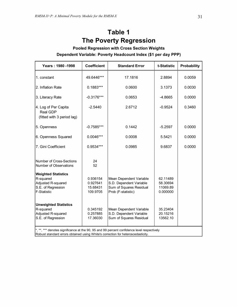
For the poverty regressions, due to that scarcity of data observations on the incidence of poverty as well as the Gini coefficient (which represents income inequality), our poverty regressions using pooled cross-section time-series data only include 24 low-income countries with 52 observations. The coverage of the regressions includes the years 1980 through 1998 (Table 1).
In contrast, we had a significantly larger number of observations for the education and health regressions. For the education regression, there were 229 observations that spanned 32 countries and covered years 1983 through 1998 (Table 2). For the health regression, there were 43 countries and a total of 174 observations. The health regression sample covered years 1990 through 1999 (Table 3). 4.1.1 Definitions of Variables Dependent Variables 1. Poverty headcount index: The percentage share (out of the total population) of
individuals earning less than the international poverty line of Purchasing Power Parity (PPP) adjusted $1.08 per day. (Source: The World Bank Global Poverty Monitoring website at http://www.worldbank.org/research/povmonitor/.)
RMSM-X+P: A Minimal Poverty Module for the RMSM-X 16
2. Adult literacy rate: The percentage of people ages 15 and above who can, with understanding, read and write a short, simple statement on their everyday life. (Source: The World Bank World Development Indicators.)
3. Infant mortality rate: The number of infants dying before reaching one year of
age, per 1,000 live births in a given year. (Source: The World Bank World Development Indicators.)
Independent Variables: Poverty Regression 1. Inflation rate: Measured by the consumer price index. Reflects the annual
percentage change in the cost to the average consumer of acquiring a fixed basket of goods and services that may be fixed or changed at specified intervals, such as yearly. The Laspeyres formula is generally used. (Source: The World Bank World Development Indicators.)
2. Literacy rate20: As defined above. 3. Per capita real GDP: Chain-weighted per capita Real GDP. (Source: Penn World
Table Version 6.1 website at http://pwt.econ.upenn.edu/.)21 To account for the very likely problem of endogeneity, we used as an instrument the previous three lagged values of per capita real GDP. To construct this instrument, we regressed with country fixed-effects per capita real GDP in time t on per capita real GDP in time t-1, t-2 and t-3, after which, the fitted values were used as the independent variable for the poverty regression22.
4. Openness: The ratio of the sum of imports of goods and services23 and exports of
goods and services24 to GDP. (Source: The World Bank World Development Indicators.)
20 Please note that this variable is a dependent variable in a health regression but appears as an independent variable in the poverty and health regressions. 21 See Heston and Summers (1991) and Heston, Summers and Aten (2002) for more details. 22 Mathematically, we initially estimated with fixed effects: log (per capita real GDP it) = β0i + β1 log (per capita real GDPi,t-1) +
β2 log (per capita real GDPi,t-2) + β3 log (per capita real GDPi,t-3)
Subsequently, we obtained predicted values of log (per capita real GDP it)that were used as an instrument for the actual log (per capita real GDP it). 23 Imports of goods and services represent the value of all goods and other market services received from the rest of the world. They include the value of merchandise, freight, insurance, transport, travel, royalties, license fees, and other services, such as communication, construction, financial, information, business, personal, and government services. They exclude labor and property income as well as transfer payments. 24 Exports of goods and services represent the value of all goods and other market services provided to the rest of the world. They include the value of merchandise, freight, insurance, transport, travel, royalties, license fees, and other services, such as communication, construction, financial, information, business, personal, and government services. They exclude labor and property income as well as transfer payments.
RMSM-X+P: A Minimal Poverty Module for the RMSM-X 17
5. Openness squared: The square of the openness term. 6. Gini coefficient: An increase in the Gini coefficient implies an increase income
inequality. The Gini index measures the extent to which the distribution of income (or, in some cases, consumption expenditure) among individuals or households within an economy deviates from a perfectly equal distribution. A Lorenz curve plots the cumulative percentages of total income received against the cumulative number of recipients, starting with the poorest individual or household. The Gini index measures the area between the Lorenz curve and a hypothetical line of absolute equality, expressed as a percentage of the maximum area under the line. Thus a Gini index of zero represents perfect equality, while an index of 100 implies perfect inequality. (Source: Dollar and Kraay, 2001.)
Independent Variables: Education Regression 1. Average per capita public education expenditure: Simple moving average of the
ratio of public education expenditure to total population in time period t, t-1, t-2, t-3. The use of the average level as opposed to the current level of public education expenditure is in recognition of the fact that the level of education, in this case being measured by the literacy rate, tends to move very slowly over time and would require a significant amount of time before increase expenditures can take effect. (Source: The World Bank World Development Indicators.)
2. Trend value of per capita real GDP: Used in the education and health regressions.
Constructed using the Hodrick-Prescott (HP) filtered25 values of the per capita real GDP.
3. Urbanization rate: The share of the total population living in areas defined as
urban in each country. (Source: The World Bank World Development Indicators.)
Independent Variables: Health Regression 1. Per capita public health expenditure: Ratio of public education expenditure to
total population. (Source: The World Bank World Development Indicators.) 2. Trend value of per capita real GDP: As defined above. 3. Literacy rate: As defined above.
25 See Hodrick and Prescott (1997).
RMSM-X+P: A Minimal Poverty Module for the RMSM-X 18
4.1.2 Econometric Methodology To investigate the significance of macroeconomic factors on the incidence of poverty, we estimate:
RMSM-X+P: A Minimal Poverty Module for the RMSM-X 19
Poverty it = β0 + β1 Inflation it + β2 Literacy Rate it + β3 log (Per capita real GDP it ) + β4 Openness it + β5 (Openness it)2 + β6 Gini it
(1) where i denotes country and t denotes year. Similarly, to access the effects of macroeconomic and structural factors on the general level of education, we estimate the Education Regression as: log (Literacy Rate it) = β0i +
β1 log (Average [Public Education Expenditure it / Popit]) + β2 log (Trend per capita real GDP it) + β3 log (Urbanization rate it)
(2) Lastly, to determine the effects of macroeconomic and structural factors on the standard of general health, we estimate the Health Regression as: log (Infant Mortality Rate it) = β0 + β1 log (Public Health Expenditure it / Popit) +
β2 log (Trend per capita real GDP it) + β3 log (Literacy rate it )
(3)
Note that the Poverty Regression was estimated using (unbalanced) panel data without country fixed-effects. Weighted Least Squares together with White’s heteroskedasticity consistent standard errors were employed. However, the Education and Health Regressions were estimated using OLS with country fixed-effects. In addition, we used White’s heteroskedasticity consistent standard errors. 4.2 Estimation Results 4.2.1 The Poverty Regression Table 1 presents the panel regression results of estimating the Poverty Equation (1) where the dependent variable is the level of the poverty headcount index. Note that the adjusted R-squared is 0.93, implying that approximately 93 percent of the variation in the dependent variable is explained by the independent variables. It was argued in the previous section that inflation was expected to have an positive effect on poverty. From the estimation results, we see that the estimated
RMSM-X+P: A Minimal Poverty Module for the RMSM-X 20
coefficient for inflation does have a positive sign that is highly statistically significant and indicates that a one percentage point increase in the inflation rate tends to increase the poverty headcount index by a 0.19 percentage point. Similarly, the estimated coefficient for the literacy rate exhibits the theoretically expected negative sign and is statistically significant at the 99 percent confidence level. We see that the estimated coefficient implies that a percentage point increase in the literacy rate leads to a 0.32 percentage point decrease in the incidence of poverty.
Recall that per capita real GDP was postulated to have a negative effect on poverty and the regression results do indicate that it has a large negative effect on the incidence of poverty, even though the estimated coefficient is not statistically significant. It is noted from Table 1 that poverty decreases by 2.54 percentage points if per capita real GDP increases by 1 percent. Given that the mean level of the poverty headcount index of the observations included in the regression sample is 35.23 percent, it can be calculated that the growth-poverty elasticity implied by our estimates is approximately -7 percent26.
The estimated coefficient of openness has the postulated negative sign and it is
statistically significant at the 99 percent confidence level. However, the estimated coefficient of the openness squared term is positive and also highly significant. This result implies that at low levels of globalization, globalization would tend to decrease poverty, but at high levels of globalization, globalization would tend to increase poverty27. At the regression sample mean level of openness of 58.45 percent, our estimated coefficients for openness and openness squared implies that a one percentage point increase in openness will decrease the poverty headcount index by 0.22 percentage point. Lastly, our results show that the estimated coefficient of the Gini index has the theoretically expected sign and is again highly significant. We see that a percentage point increase in the Gini coefficient tends to increase poverty by 0.95 percentage point.
As simple robustness checks, we also estimated regressions where the instrument for the logged of real GDP per capita was replaced with predicted values of logged of
26 A growth-poverty elasticity of -7 percent is significantly higher than what has been previously found in by Ravallion and Chen (2000), which was –3.1 percent. One possible explanation for the larger growth-poverty elasticity is that our sample of countries includes only low-income countries. It is very plausible that these countries have much higher returns to economic growth in terms of poverty reduction. Recall that Gallup, Radelet and Warner (1999) also found that the growth elasticity of the average income of the bottom quintile of the income distribution was significant higher for low-income countries as compared to a global sample. 27 This result is in sharp contrast to the findings of Agenor (2003). Recall that he found that the coefficient of the first-order globalization term was negative, while the coefficient of the second-order term was positive. Thus his results implied that at low levels of globalization, globalization would tend to increase poverty, but at high levels of globalization, globalization would tend to decrease poverty. Again, recall that our estimates pertain exclusive to low-income countries, and as such, it is conceivable that poverty alleviation in low-income countries resulting from international trade may experience a degree of diminishing returns. Note that this result of diminishing returns to international trade was strongly robust to various regressions specifications examined for this paper.
RMSM-X+P: A Minimal Poverty Module for the RMSM-X 21
real GDP per capita estimated from regressions that included only 1 or 2 lagged periods. Tables 1a and 1b present the results and we see that they are qualitatively and quantitatively similar to those in Table 1.
4.2.2 The Education Regression Table 2 presents the results for the education regression where the dependent variable is the log of the adult literacy rate. With an adjusted R-squared of 0.99, the three independent variables, namely log of average per capita public education expenditure, log of real GDP per capita trend28 and the log of the urbanization ratio, together with the country fixed effects, account for most of the variation of the literacy rate across time and countries.
In addition, we see that all of the explanatory variables possess estimated coefficients that are of the postulated positive sign and are highly statistically significant. We observe that a 1 percent increase in the average public educational expenditure share leads to a 0.02 percent increase in the literacy rate. Similarly, a 1 percent increase in the trend value of real GDP per capita, or the standard of living, tends to increase the literacy rate by 0.09 percent, and 1 percent increase in the urban population share leads to a 0.85 percent increase in the literacy rate.
Recall that the public education expenditure variable here is constructed as the simple moving average of the ratio of public education expenditure to total population in time period t, t-1, t-2, t-3. Some may argue that the choice of this four-period moving average is very arbitrary. Therefore as another robustness check, an alternative regression with the public education expenditure variable being constructed as an average over periods t through t-4, were estimated. Table 2a shows that results were qualitatively somewhat similar, with the exception of a decrease in the level of significance for 2 of the coefficients. We attribute this decrease in significance to the substantial decrease in the number of degrees of freedom as compared to the first education regression. 4.2.3 The Health Regression The regression results for the health regression where the dependent variable is the log of the infant mortality rate are presented in Table 3. As with the education regression, the 3 independent variables, together with the country fixed effects account for most of the cross-country intertemporal variation of the infant mortality rate (99 percent). All independent variables have coefficients of the theoretically expected negative sign. While the public health expenditure and the literacy rate variables have
28 This variable can be interpreted as the standard of living.
RMSM-X+P: A Minimal Poverty Module for the RMSM-X 22
highly significant coefficients, the real GDP per capita variable has an estimated coefficient that is significant at the 90 percent confidence interval.
In terms of the quantitative results, the estimated coefficient of public health expenditure implies that the elasticity of the infant mortality rate with respect to public health expenditure is –0.0229,30.
Similarly, the estimated coefficient of –0.11 for the real GDP variable implies that
a 1 percent increase in the real GDP per capita variable leads to a 0.11 percent decrease in the infant mortality rate. Lastly, the results indicate that a 1 percent increase in the literacy rate tends to decrease the infant mortality rate by 0.60 percent. 5. Linking the Poverty Module with the RMSM-X 5.1 The Detailed Structure of the Poverty Module
In the RMSM-X+P model, projections of the impact of macroeconomic policies on poverty are carried out in the poverty sheet of the Poverty Module, which is linked to the Macroeconomic Module (RX-XP.xls) of the standard RMSM-X.
The Poverty Module follows standard RMSM-X coloring conventions for cells in
worksheets (Figure 3): • Light blue - actual base-year data • Green - estimated coefficients (elasticities) in equations and assumptions • Yellow - actual data, which are input from other parts of RMSM-X model
29 While this estimated coefficient suggests a relatively small elasticity of the average health level with
respect to public health expenditure, it does produce the intuitive result of a positive and statistically significant effect of education level on education. This is in contrast to several previous studies where there were significant positive effects on public education expenditure on the average education levels. For example, see Filmer and Pritchett (1999).
30 As in the case of education regression, we recognize that there are long-term effects extending from public health expenditures to the level of health of the population. However, when the current period public health expenditure variable was replaced with one that was averaged over the current period and period t-1, most of the independent variables returned coefficients that were quantitatively similar but exhibited reduced statistical significance (Table 3a). We therefore attribute this abrupt change in the statistical significance of the estimated coefficients to the sharp decrease in the number of observations in the new regression sample. As an additional robustness test for the possible medium-term effects of public expenditure on health levels, we investigated the effects of lagged per capita public health expenditure on the infant mortality rate (Table 3b) and found similar results as those in Table 3 but the estimated coefficients were less significant.
RMSM-X+P: A Minimal Poverty Module for the RMSM-X 23
• Uncolored cell - are either empty or contain automatically calculated formulae. Data should not be entered into the uncolored cells to avoid overwriting existing formulae.
The Poverty Module, which is an Excel file, includes three worksheets: poverty,
education, and health worksheets. These worksheets follow a standard format as follows:
1. Original data entry for chosen base year • Poverty worksheet: base-year actual (known) poverty headcount and Gini
coefficient • Education worksheet: base-year actual (known) literacy rate, average per
capita public expenditures, share of education expenditures in public expenditures, and urbanization ratio
• Health worksheet: base-year actual (known) infant mortality rate and average per capita public expenditures, and share of health expenditures in public expenditures
2. Regression coefficients for the variables identified in each of the chosen
equations described in the paper • The coefficients (elasticities) were estimated using econometric techniques
based on a representative multi-country, multi-year sample and are assumed to remain constant over the entire projections period. These coefficients are not expected to be changed by the user unless they are re-estimated with a new sample either based on panel data or time series data for the country under study.
3. Assumptions on exogenous variables
• Poverty, Education, and Health worksheets: for projections years, designated macroeconomic variables from RMSM-X or other model and assumptions about the projected values of relevant exogenous variables.
4. Projected results for the identified indicators
• Poverty worksheet: poverty headcount. • Education worksheet: literacy rate. • Health worksheet: infant mortality rate.
5. Working area in each of the worksheets to check the accuracy of the projected
values from the equations. These are provided for the user to check the contribution arising from each of the exogenous terms shown in the particular equation under consideration.
6. Relevant charts pertaining to each of the results indicators: poverty
headcount, literacy rate and infant mortality.
RMSM-X+P: A Minimal Poverty Module for the RMSM-X 24
5.2 Linking the Poverty Module to the standard RMSM-X
There is no unique way to link the poverty module to the RMSM-X model. The links can vary depending on the structure of the RMSM-X or other model. The links in the current version of the poverty module are based on a standard structure of the RMSM-X model. In this case, to link the poverty module to another RMSM-X (say, for example, for another country), one can use the Edit drop down menu. The chain of commands runs as follows: Edit, link, highlight current link, click on “change links” and specify the location of the subdirectory where the desired RMSM-X model could be found.
More recent versions of the RMSM-X available, including the “mini” model are now available. Since the location of the required variables in RMSM-X models can vary, it may be feasible to manually link the two modules. This can easily be done as the number of variables to be linked is very small. Users who find it convenient to bring the poverty module into the RMSM-X can do so by moving the 3 worksheets in question into the main body of the RMSM-X model. One can do this before or after linking the sheets as described above. If these 3 worksheets are brought into the RMSM-X model before linking, it would be necessary to change the links (as described above, or manually) after the worksheets are brought in. The downside of adding 3 more worksheets to the existing RMSM-X is that the size of the Excel file would increase somewhat. This is not a problem in most cases, given the current status of spreadsheet capabilities.
The indicators in the poverty module that need to be linked to the RMSM-X model
are: GDP per capita at constant LCU (row 18, poverty worksheet) GDP deflator (row 17, poverty worksheet) Openness indicator (row 19, poverty worksheet) Total government expenditures per capita (row 18, education worksheet)
6. Analysis with RMSM-X+P: An Example In this section, we present an example where the RMSM-X+P is used to analyze the effects of an increase in the share of public education expenditure in total government expenditure on education, health and poverty. This exercise is performed using our prototype RMSM-X+P that has not been calibrated for any specific country.
RMSM-X+P: A Minimal Poverty Module for the RMSM-X 25
6.1 Changing Public Spending on Education Figure 4 presents the education worksheet as we can see that the share of public education expenditure is constant at 15 percent of total government expenditure from 2003 to 2010 and this corresponds to the literacy rate of 85 percent in 2003 and increasing to 89.6 percent in 2010. Figure 5 shows the corresponding base-run plot of the literacy rate. For the same time period, we see that the poverty headcount index decreases from 50 percent to 20.7 percent (Figure 6) and the infant mortality rate decreases from 50 to 45.9 deaths per 1,000 live births (Figure 7).
Now suppose that the share of total government expenditures devoted to education is doubled to 30 percent beginning in the year 2004. As a result of this change, the literacy rate improves as shown by the curve representing the “current” scenario. Because the literacy rate is also a determinant of the poverty head count, the latter is also re-calculated automatically in the poverty module. The corresponding graph for the poverty headcount shows both a “baseline” and a “current” scenario corresponding to this change in assumption of education expenditures.
From Figure 8, we see the increase in public education expenditure share leads to new literacy rates, represented by the “current” scenario, being all consistently higher than the baseline values for the years 2003 through 2010. The projected literacy rate in 2010 is now 91.0 percent as opposed to the baseline 2010 value of 89.6 percent. Because the literacy rate is also a determinant of the poverty headcount index, the latter is also re-calculated automatically in the poverty sheet. The increase in the literacy rate leads to small decrease in the incidence poverty (Figure 9) where it decreased from a baseline value of 20.7 percent to 20.2 percent in year 2010. Similarly, given that the literacy rate is a determinant of the infant mortality rate, the latter decreases with the increase of the former as shown in Figure 10. The infant mortality rate falls from the 2010 baseline value of 45.9 to 45.5. We see that from the above exercise that an increase in the share of government expenditure on education results in an increase in the literacy rate, which consequently leads to a decrease in poverty and infant mortality rate. The rather small magnitude of the decrease in poverty may suggest that attempting to fight poverty solely by increasing the general level of education may not be sufficient and that a multiple faceted approach may be warranted.
Similar simulations can be carried out with respect to changes in any of the explanatory variables in each of the poverty, education and health equations considered in the Poverty Module. Note that the Module contains a facility to save a “baseline” scenario, which facilitates the generation of the graphs to see the impact of alternative assumptions on the three social sector indicators considered in the Poverty Module.
RMSM-X+P: A Minimal Poverty Module for the RMSM-X 26
7. Concluding Remarks
The RMSM-X+P is a new tool that allows the RMSM-X to perform analysis on the effects of macroeconomic shocks on poverty, education and health. It incorporates a Poverty Module that contains equations that link key macroeconomic, structural and policy variables to the poverty headcount index, the literacy rate, and the infant mortality rate. More specifically, the poverty equation links the incidence of poverty to inflation, the literacy rate, real GDP per capita, the degree of openness and income inequality. Similarly, the education equation depicts the effects of public education expenditure, real GDP per capita and urbanization on the literacy rate. Lastly, the health equation links the infant mortality rate to public health expenditure, per capita real GDP and the literacy rate. These equations thus enable the changes in poverty, education and health due to changes in macroeconomic or policy variables to be projected.
Each of the equations was empirically estimated using cross-country panel
regressions based on historical data for low-income countries, which determined the magnitudes of the effects of the above-mentioned macroeconomic, structural and policy variables on poverty, education and health. The resulting parameter estimates are then combined with macroeconomic projections from the RMSM-X model and assumptions about other exogenous (structural) variables to obtain projections for the indicators.
Although the RMSM-X+P allows the user to address a limited set of policy
issues, it has a number of advantages, perhaps the most substantial being that it permits a move beyond the rather simplistic focus on the partial correlation between growth and poverty in our discussions of poverty reduction.
RMSM-X+P: A Minimal Poverty Module for the RMSM-X 27
References Agénor, Pierre-Richard. “Macroeconomic Adjustment and the Poor: Analytical
Issues and Cross-Section Evidence.” Policy Research Working Paper No. 2788, The World Bank, August 2002. Forthcoming, Journal of Economic Surveys.
Agénor, Pierre-Richard, Alejandro Izquierdo and Hippolyte Fofack. “IMMPA:
An integrated Macroeconomic Framework for the Analysis of Poverty Reduction Strategies,” Policy Research Working Paper No. 3092, World Bank (June 2003).
Agénor, Pierre-Richard. “Does Globalization Hurt the Poor?” Journal of
International Economics and Economic Policy. Vol. 1 (January 2004a), 1-31. Agénor, Pierre-Richard. The Economics of Adjustment and Growth. 2nd ed.,
forthcoming, Harvard University Press (Boston, Mass.: 2004b). Aghion, Philippe, Eva Caroli and Cecilia Garcia-Penalosa. “Inequality and
Growth: The Perspective of the New Growth Theories.” Journal of Economic Literature. Vol. 37, December 1999, pp. 1615-1660.
Alesina, Alberto and Roberto Perotti. “Income Distribution, Political Instability
and Investment.” European Economic Review. Vol. 40, 1996, pp. 1203-1228. Anand, Sudhir and Martin Ravallion (1993). “Human Development in Poor
Countries: On the Role of Private Incomes and Public Services.” Journal of Economic Perspectives. Vol. 7, No. 1 (Winter), pp. 133-150.
Bruno, Michael, Martin Ravallion and Lyn Squire. “Equity and Growth in
Developing Countries: Old and New Perspectives on the Policy Issues.” Policy Research Working Paper No. 1563, The World Bank, January 1996.
Bulir, Ales and Anee-Marie Gulde. “Inflation and Income Distribution: Further
Evidence on Empirical Links.” Working Paper No. 95/86, International Monetary Fund, August 1995.
Caldwell, John C. (1990). “Cultural and Social Factors Influencing Mortality
Levels in Developing Countries.” The Annals of the American Academy of Political and Social Science. Vol. 510 (July), pp. 44-59. Choi, Sangmok, Bruce D. Smith and John H. Boyd. “Inflation, Financial Markets, and Capital Formation.” Review. Federal Reserve Bank of St. Louis, May 1996, pp. 9-35.
RMSM-X+P: A Minimal Poverty Module for the RMSM-X 28
De Gregorio, José and Jong-Wha Lee (1999). “Education and Income Distribution: New Evidence from Cross Country Data.” Harvard Institute for International Development (HIID) Development Discussion Paper No. 714, July. Demery, Lionel and Lyn Squire. “Macroeconomic Adjustment and Poverty in Africa: An Emerging Picture.” World Bank Research Observer. Vol. 11, February 1996, pp. 35-59.
Dollar, David and Aart Kraay. “Trade, Growth, and Poverty.” Policy Research Working Paper 2615, The World Bank, June 2001. Dollar, David and Aart Kraay. “Growth is Good for the Poor.” Journal of Economic Growth. Vol. 7, No. 3, September 2002, pp. 195-225. Dorosh, Paul A. and David E. Sahn. “A General Equilibrium Analysis of the Effect of Macroeconomic Adjustment on Poverty on Africa.” Journal of Policy Modeling. Vol. 22, November 2000, pp. 753-776. Easterly, William and Stanley Fischer. “Inflation and the Poor.” Journal of Money Credit and Banking. Vol. 33, No. 2, May 2001, pp. 160-178. Flegg, A. T. (1982). “Inequality of Income, Illiteracy and Medical Care as Determinants of Infant Mortality in Underdeveloped Countries.” Population Studies. Vol. 36, No. 3, pp. 441-458.
Frankel, Jeffrey A., and David Romer. “Does Trade Cause Growth.” The American Economic Review. Vol. 89, No. 3, June 1999, pp. 379-399.
Foster, James E. and Miguel Székely. “Is Economic Growth Good for the Poor?
Tracking Low Incomes Using General Means.” Working Paper No. 453, Research Department, The Inter-American Development Bank, June 2001 Filmer, Deon and Lant Pritchett. “The Impact of Public Spending on Health: Does Money Matter ?” Social Science and Medicine. Vol. 49, 1993, pp. 1309-1323. Galor, Oded and Joseph Zeira. “Income Distribution and Macroeconomics.” Review of Economic Studies. Vol. 60, January 1993, pp. 35-52. Gallup, John Luke, Steven Radelet and Andrew Warner. “Economic Growth and the Income of the Poor.” Consulting Assistance on Economic Reform II (CAER II) Discussion Paper No. 36. Harvard Institute for International Development, January 1999.
RMSM-X+P: A Minimal Poverty Module for the RMSM-X 29
Greenaway, David, Wyn Morgan and Peter Wright. “Trade Liberalisation and Growth in Developing Countries.” Journal of Development Economics. Vol. 67, No. 1 (February 2002), pp. 229-244. Gundlach, Erich, José Navarro de Pablo and Natascha Weisert. “Education is Good for the Poor: A Note on Dollar Kraay (2001).” World Institute for Development Economics Research (WIDER) Discussion Paper No. 2001/137, November 2001.
Heston, Alan and Robert Summers (1991). “The Penn World Table (Mark 5) : An Expanded Set of International Comparisons, 1950-1988.” Quarterly Journal Economics. May, pp. 327-368.
Heston, Alan, Robert Summers and Bettina Aten (2002). Penn World Table
Version 6.1. Center for International Comparisons at the University of Pennsylvania (CICUP), October.
Hodrick, Robert J. and Edward C. Prescott (1997). “Postwar U.S. Business
Cycles: An Empirical Investigation.” Journal of Money, Credit and Banking. Vol. 29, No. 1 (February), pp. 1-16.
Irwin, Douglas A. and Marko Tervio. “Does Trade Raise Income? Evidence
form the Twentieth Century.” Journal of International Economics. Vol. 58, 2002, pp. 1-18.
Kakwani, N. “Performance in Living Standards: An International Comparison.” Journal of Development Economics. Vol. 41, No. 2, pp. 307-336, 1993. Lora, Eduardo and Mauricio Oliveria. “Macro Policy and Employment Problems in Latin America.” Working Paper No. 372, Inter-American Development Bank, March 1998. Pritchett, Lant and Lawrence H. Summers (1996). “Wealthier is Healthier.” Journal of Human Resources. Vol. 31, No. 4, pp. 841-868. Ravallion, Martin and Shao-Hua Chen (1997). “What can Survey Data tell us about Recent Changes in Distribution and Poverty?” World Bank Economic Review. Vol. 11, No. 2 (May), pp. 357-382 Roemer, Michael and Mary Kay Gugerty. “Does Economic Growth Reduce Poverty.” Consulting Assistance on Economic Reform II (CAER II) Discussion Paper No. 4. Harvard Institute for International Development, January 1997. Romer, Christina and David Romer. “Monetary Policy and the Well-Being of the Poor.” National Bureau of Economic Research Working Paper 6793, November 1998.
RMSM-X+P: A Minimal Poverty Module for the RMSM-X 30
Sachs, Jeffrey D. and Andrew M. Warner (1995). “Economic Reform and the Process of Global Integration.” Brookings Papers on Economic Activity. Vol. 1 (August), pp. 1-118. Sahn, David E., Paul A. Dorosh and Stephen D. Younger. Structural Adjustment Reconsidered: Economic Policy and Poverty in Africa. Cambridge University Press, Cambridge 1997. Servén, Luis. “Uncertainty, Instability and Irreversible Investment: Theory, Evidence and Lessons for Africa.” PRE Working Paper No. 1722, The World Bank, February 1997. -----. “Macroeconomic Uncertainty and Private Investment in Developing Countries.” PRE Working Paper No. 2035, the World Bank, December 1998. Timmer, C. Peter. “How Well Do the Poor Connect to the Growth Process?” Consulting Assistance on Economic Reform II (CAER II) Discussion Paper No. 17. Harvard Institute for International Development, January 1997. World Bank (2000a). Attacking Poverty: World Development Report 2000. The World Bank, Washington DC. World Bank (2000b). The Quality of Growth. The World Bank, Washington DC. World Bank (2000c). “Empirics of the Link Between Growth and Poverty.” PREM Notes. No. 45 (October). The World Bank, Washington DC.
Zeufack, Albert G. “Structure de propriété et comportement d’investissement en environnement incertain.” Revue d’Economie du Développement. March 1997, pp. 29-59.
RMSM-X+P: A Minimal Poverty Module for the RMSM-X 31
Years : 1980 -1998 Coefficient Standard Error t-Statistic Probability
1. constant 49.6446*** 17.1816 2.8894 0.0059
2. Inflation Rate 0.1883*** 0.0600 3.1373 0.0030
3. Literacy Rate -0.3176*** 0.0653 -4.8665 0.0000
4. Log of Per Capita -2.5440 2.6712 -0.9524 0.3460 Real GDP (fitted with 3 period lag)
5. Openness -0.7585*** 0.1442 -5.2597 0.0000
6. Openness Squared 0.0046*** 0.0008 5.5421 0.0000
7. Gini Coefficient 0.9534*** 0.0985 9.6837 0.0000
Number of Cross-Sections 24Number of Observations 52
Weighted StatisticsR-squared 0.936154 Mean Dependent Variable 62.11489Adjusted R-squared 0.927641 S.D. Dependent Variable 58.30694S.E. of Regression 15.68431 Sum of Squares Residual 11069.89F-Statistic 109.9705 Prob (F-statistic) 0.000000
Unweighted StatisticsR-squared 0.345192 Mean Dependent Variable 35.23404Adjusted R-squared 0.257885 S.D. Dependent Variable 20.15216S.E. of Regression 17.36030 Sum of Squares Residual 13562.10
*, **, *** denotes significance at the 90, 95 and 99 percent confidence level respectivelyRobust standard errors obtained using White's correction for heteroscedasticity.
Table 1The Poverty Regression
Pooled Regression with Cross Section WeightsDependent Variable: Poverty Headcount Index ($1 per day PPP)
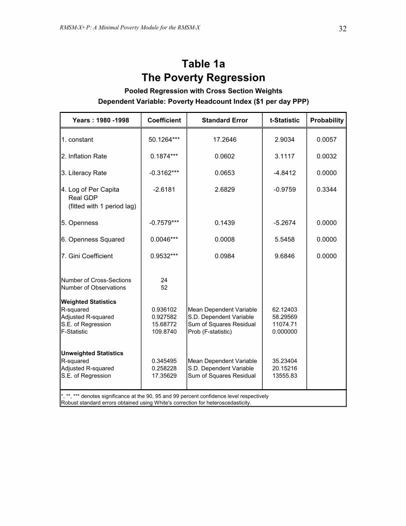
RMSM-X+P: A Minimal Poverty Module for the RMSM-X 32
Years : 1980 -1998 Coefficient Standard Error t-Statistic Probability
1. constant 50.1264*** 17.2646 2.9034 0.0057
2. Inflation Rate 0.1874*** 0.0602 3.1117 0.0032
3. Literacy Rate -0.3162*** 0.0653 -4.8412 0.0000
4. Log of Per Capita -2.6181 2.6829 -0.9759 0.3344 Real GDP (fitted with 1 period lag)
5. Openness -0.7579*** 0.1439 -5.2674 0.0000
6. Openness Squared 0.0046*** 0.0008 5.5458 0.0000
7. Gini Coefficient 0.9532*** 0.0984 9.6846 0.0000
Number of Cross-Sections 24Number of Observations 52
Weighted StatisticsR-squared 0.936102 Mean Dependent Variable 62.12403Adjusted R-squared 0.927582 S.D. Dependent Variable 58.29569S.E. of Regression 15.68772 Sum of Squares Residual 11074.71F-Statistic 109.8740 Prob (F-statistic) 0.000000
Unweighted StatisticsR-squared 0.345495 Mean Dependent Variable 35.23404Adjusted R-squared 0.258228 S.D. Dependent Variable 20.15216S.E. of Regression 17.35629 Sum of Squares Residual 13555.83
*, **, *** denotes significance at the 90, 95 and 99 percent confidence level respectivelyRobust standard errors obtained using White's correction for heteroscedasticity.
Table 1aThe Poverty Regression
Pooled Regression with Cross Section WeightsDependent Variable: Poverty Headcount Index ($1 per day PPP)
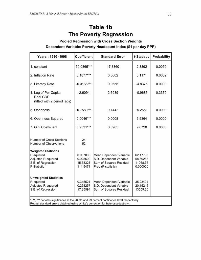
RMSM-X+P: A Minimal Poverty Module for the RMSM-X 33
Years : 1980 -1998 Coefficient Standard Error t-Statistic Probability
1. constant 50.0865*** 17.3360 2.8892 0.0059
2. Inflation Rate 0.1877*** 0.0602 3.1171 0.0032
3. Literacy Rate -0.3166*** 0.0655 -4.8375 0.0000
4. Log of Per Capita -2.6094 2.6939 -0.9686 0.3379 Real GDP (fitted with 2 period lags)
5. Openness -0.7580*** 0.1442 -5.2551 0.0000
6. Openness Squared 0.0046*** 0.0008 5.5364 0.0000
7. Gini Coefficient 0.9531*** 0.0985 9.6728 0.0000
Number of Cross-Sections 24Number of Observations 52
Weighted StatisticsR-squared 0.937000 Mean Dependent Variable 62.17736Adjusted R-squared 0.928600 S.D. Dependent Variable 58.69288S.E. of Regression 15.68323 Sum of Squares Residual 11068.36F-Statistic 111.5471 Prob (F-statistic) 0.000000
Unweighted StatisticsR-squared 0.345521 Mean Dependent Variable 35.23404Adjusted R-squared 0.258257 S.D. Dependent Variable 20.15216S.E. of Regression 17.35594 Sum of Squares Residual 13555.30
*, **, *** denotes significance at the 90, 95 and 99 percent confidence level respectivelyRobust standard errors obtained using White's correction for heteroscedasticity.
Table 1bThe Poverty Regression
Pooled Regression with Cross Section WeightsDependent Variable: Poverty Headcount Index ($1 per day PPP)
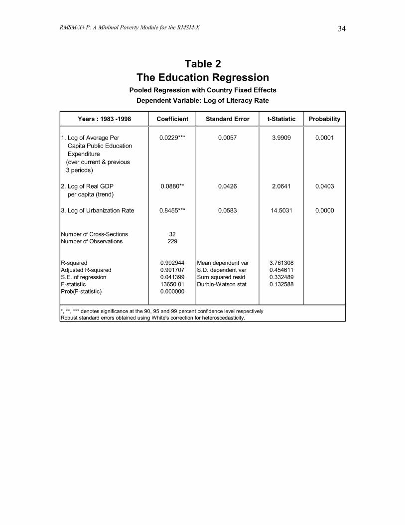
RMSM-X+P: A Minimal Poverty Module for the RMSM-X 34
Years : 1983 -1998 Coefficient Standard Error t-Statistic Probability
1. Log of Average Per 0.0229*** 0.0057 3.9909 0.0001 Capita Public Education Expenditure (over current & previous 3 periods)
2. Log of Real GDP 0.0880** 0.0426 2.0641 0.0403 per capita (trend)
3. Log of Urbanization Rate 0.8455*** 0.0583 14.5031 0.0000
Number of Cross-Sections 32Number of Observations 229
R-squared 0.992944 Mean dependent var 3.761308Adjusted R-squared 0.991707 S.D. dependent var 0.454611S.E. of regression 0.041399 Sum squared resid 0.332489F-statistic 13650.01 Durbin-Watson stat 0.132588Prob(F-statistic) 0.000000
*, **, *** denotes significance at the 90, 95 and 99 percent confidence level respectivelyRobust standard errors obtained using White's correction for heteroscedasticity.
Table 2The Education Regression
Pooled Regression with Country Fixed EffectsDependent Variable: Log of Literacy Rate

RMSM-X+P: A Minimal Poverty Module for the RMSM-X 35
Years : 1983 -1998 Coefficient Standard Error t-Statistic Probability
1. Log of Average Per 0.0251*** 0.0056 4.4949 0.0000 Capita Public Education Expenditure (over current & previous 4 periods)
2. Log of Real GDP 0.0941** 0.0430 2.1890 0.0301 per capita (trend)
3. Log of Urbanization Rate 0.8747*** 0.0662 13.2093 0.0000
Number of Cross-Sections 28Number of Observations 190
R-squared 0.994387 Mean dependent var 3.767409Adjusted R-squared 0.993328 S.D. dependent var 0.446035S.E. of regression 0.036433 Sum squared resid 0.211052F-statistic 14084.21 Durbin-Watson stat 0.168012Prob(F-statistic) 0.000000
*, **, *** denotes significance at the 90, 95 and 99 percent confidence level respectivelyRobust standard errors obtained using White's correction for heteroscedasticity.
Table 2aThe Education Regression
Pooled Regression with Country Fixed EffectsDependent Variable: Log of Literacy Rate
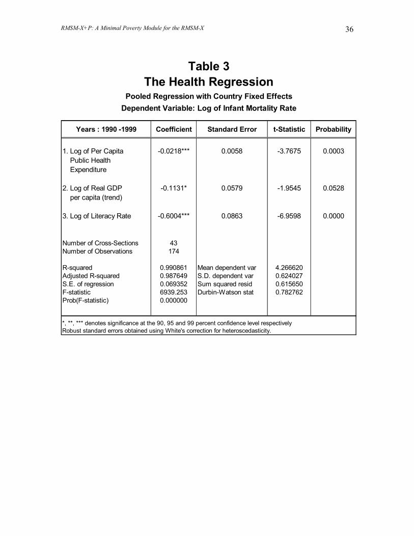
RMSM-X+P: A Minimal Poverty Module for the RMSM-X 36
Years : 1990 -1999 Coefficient Standard Error t-Statistic Probability
1. Log of Per Capita -0.0218*** 0.0058 -3.7675 0.0003 Public Health Expenditure
2. Log of Real GDP -0.1131* 0.0579 -1.9545 0.0528 per capita (trend)
3. Log of Literacy Rate -0.6004*** 0.0863 -6.9598 0.0000
Number of Cross-Sections 43Number of Observations 174
R-squared 0.990861 Mean dependent var 4.266620Adjusted R-squared 0.987649 S.D. dependent var 0.624027S.E. of regression 0.069352 Sum squared resid 0.615650F-statistic 6939.253 Durbin-Watson stat 0.782762Prob(F-statistic) 0.000000
*, **, *** denotes significance at the 90, 95 and 99 percent confidence level respectivelyRobust standard errors obtained using White's correction for heteroscedasticity.
Table 3The Health Regression
Pooled Regression with Country Fixed EffectsDependent Variable: Log of Infant Mortality Rate
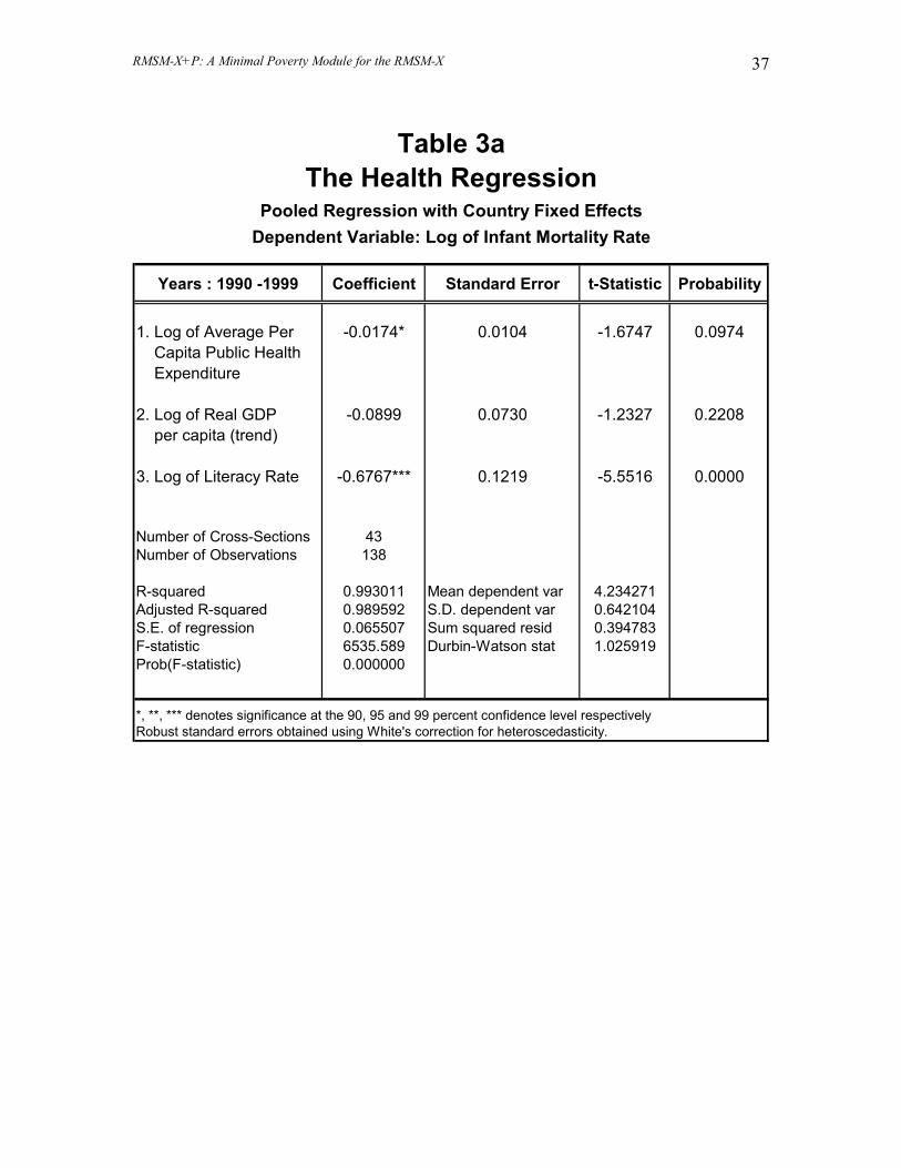
RMSM-X+P: A Minimal Poverty Module for the RMSM-X 37
Years : 1990 -1999 Coefficient Standard Error t-Statistic Probability
1. Log of Average Per -0.0174* 0.0104 -1.6747 0.0974 Capita Public Health Expenditure
2. Log of Real GDP -0.0899 0.0730 -1.2327 0.2208 per capita (trend)
3. Log of Literacy Rate -0.6767*** 0.1219 -5.5516 0.0000
Number of Cross-Sections 43Number of Observations 138
R-squared 0.993011 Mean dependent var 4.234271Adjusted R-squared 0.989592 S.D. dependent var 0.642104S.E. of regression 0.065507 Sum squared resid 0.394783F-statistic 6535.589 Durbin-Watson stat 1.025919Prob(F-statistic) 0.000000
*, **, *** denotes significance at the 90, 95 and 99 percent confidence level respectivelyRobust standard errors obtained using White's correction for heteroscedasticity.
Table 3aThe Health Regression
Pooled Regression with Country Fixed EffectsDependent Variable: Log of Infant Mortality Rate
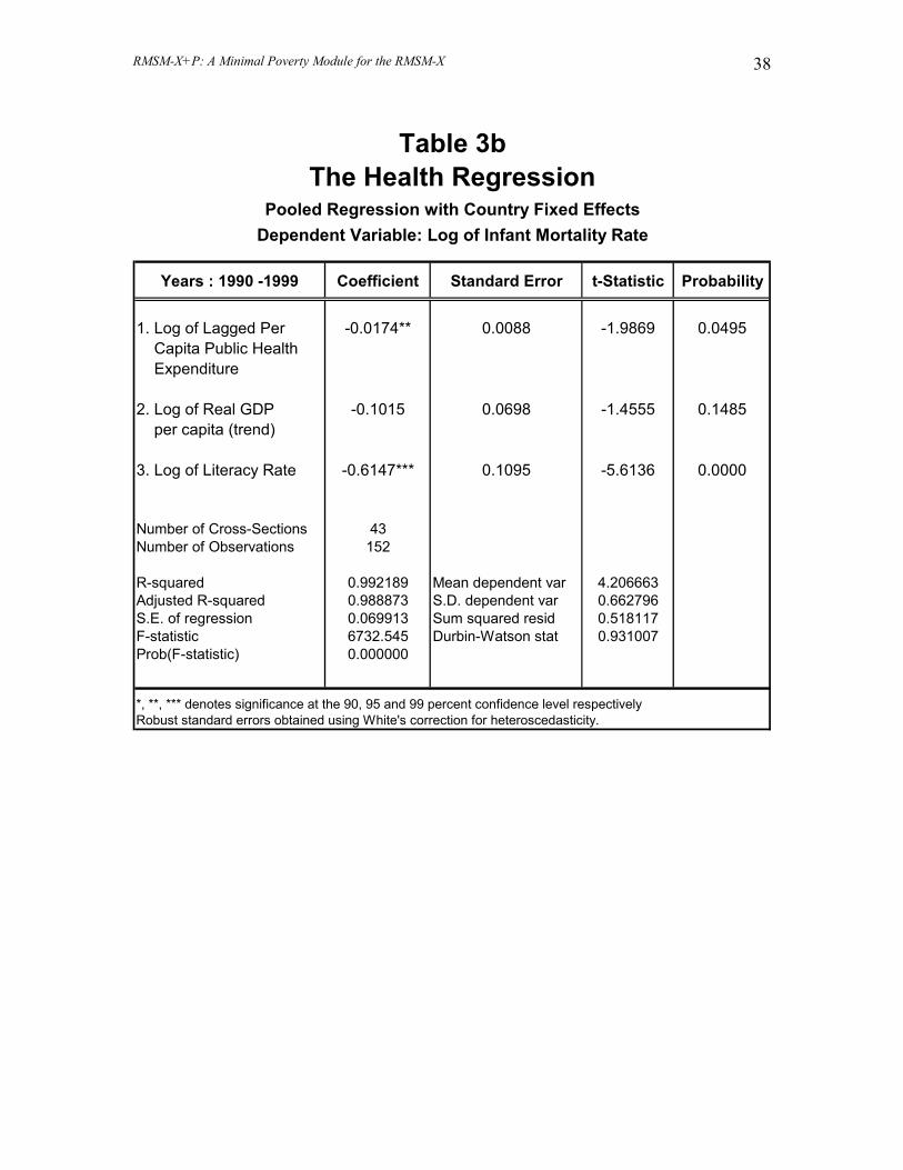
RMSM-X+P: A Minimal Poverty Module for the RMSM-X 38
Years : 1990 -1999 Coefficient Standard Error t-Statistic Probability
1. Log of Lagged Per -0.0174** 0.0088 -1.9869 0.0495 Capita Public Health Expenditure
2. Log of Real GDP -0.1015 0.0698 -1.4555 0.1485 per capita (trend)
3. Log of Literacy Rate -0.6147*** 0.1095 -5.6136 0.0000
Number of Cross-Sections 43Number of Observations 152
R-squared 0.992189 Mean dependent var 4.206663Adjusted R-squared 0.988873 S.D. dependent var 0.662796S.E. of regression 0.069913 Sum squared resid 0.518117F-statistic 6732.545 Durbin-Watson stat 0.931007Prob(F-statistic) 0.000000
*, **, *** denotes significance at the 90, 95 and 99 percent confidence level respectivelyRobust standard errors obtained using White's correction for heteroscedasticity.
Table 3bThe Health Regression
Pooled Regression with Country Fixed EffectsDependent Variable: Log of Infant Mortality Rate
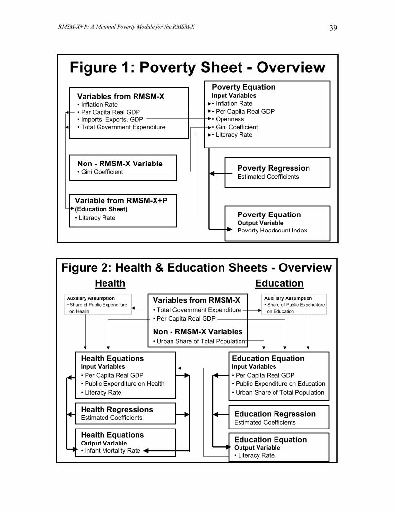
RMSM-X+P: A Minimal Poverty Module for the RMSM-X 39
Figure 2: Health & Education Sheets - Overview
Variables from RMSM-X• Total Government Expenditure• Per Capita Real GDP
Non - RMSM-X Variables• Urban Share of Total Population
Education EquationInput Variables• Per Capita Real GDP• Public Expenditure on Education• Urban Share of Total Population
Auxiliary Assumption• Share of Public Expenditure
on Education
Education EquationOutput Variable• Literacy Rate
Education RegressionEstimated Coefficients
EducationHealthAuxiliary Assumption• Share of Public Expenditure
on Health
Health EquationsInput Variables• Per Capita Real GDP• Public Expenditure on Health• Literacy Rate
Health RegressionsEstimated Coefficients
Health EquationsOutput Variable• Infant Mortality Rate
Figure 1: Poverty Sheet - OverviewVariables from RMSM-X• Inflation Rate• Per Capita Real GDP• Imports, Exports, GDP• Total Government Expenditure
Poverty EquationInput Variables• Inflation Rate• Per Capita Real GDP• Openness• Gini Coefficient• Literacy Rate
Variable from RMSM-X+P(Education Sheet)• Literacy Rate Poverty Equation
Output VariablePoverty Headcount Index
Poverty RegressionEstimated Coefficients
Non - RMSM-X Variable• Gini Coefficient
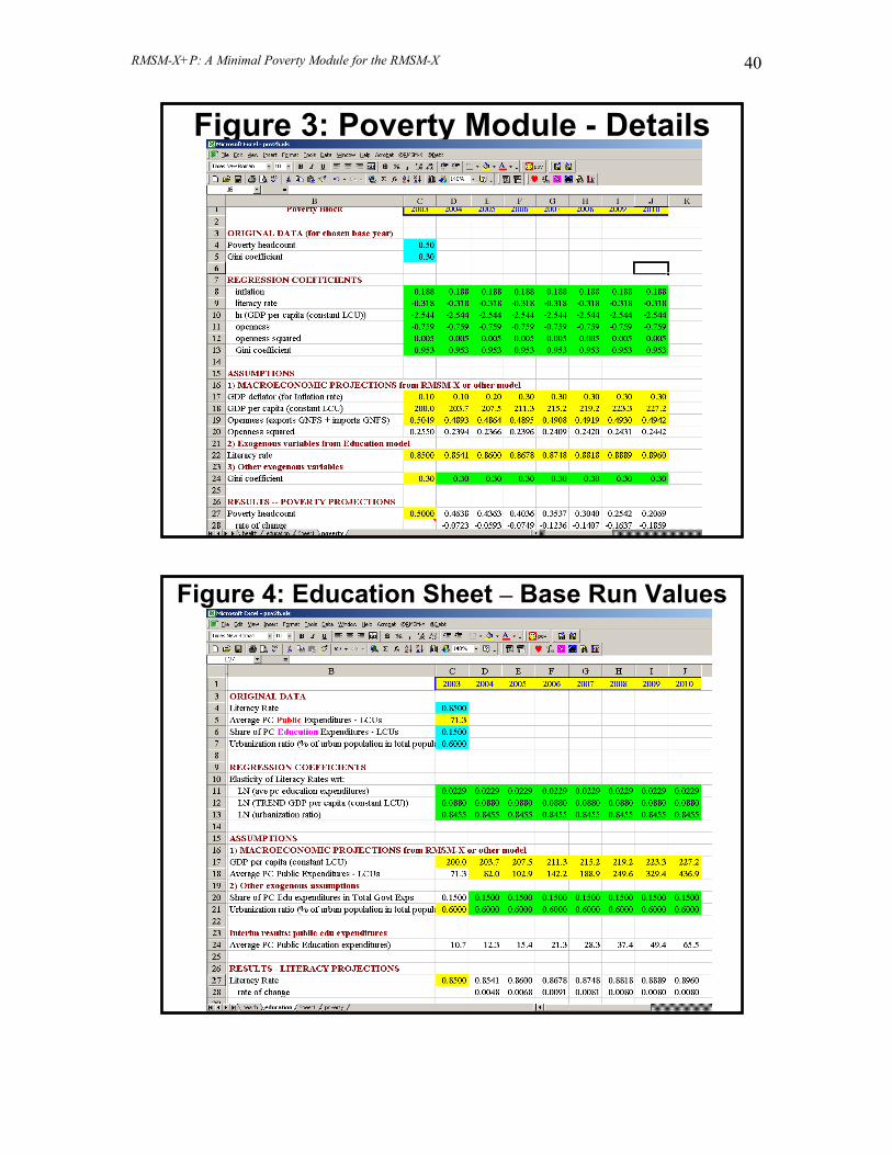
RMSM-X+P: A Minimal Poverty Module for the RMSM-X 40
Figure 3: Poverty Module - Details
Figure 4: Education Sheet – Base Run Values
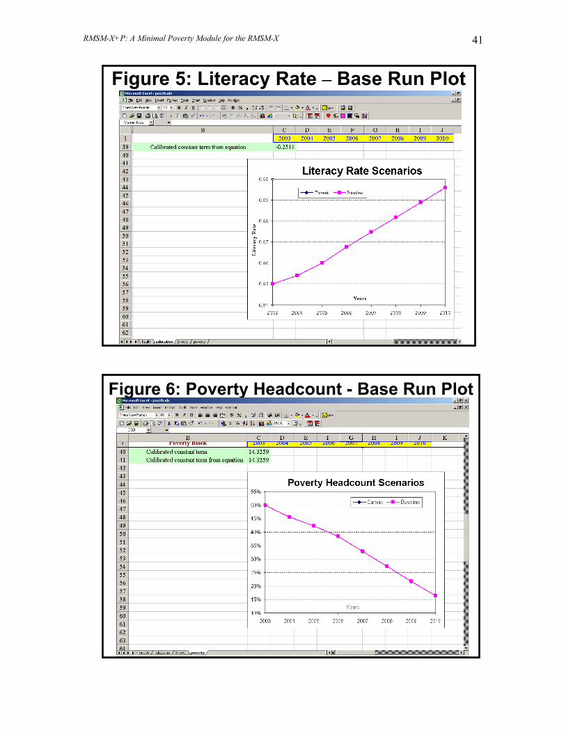
RMSM-X+P: A Minimal Poverty Module for the RMSM-X 41
Figure 5: Literacy Rate – Base Run Plot
Figure 6: Poverty Headcount - Base Run Plot
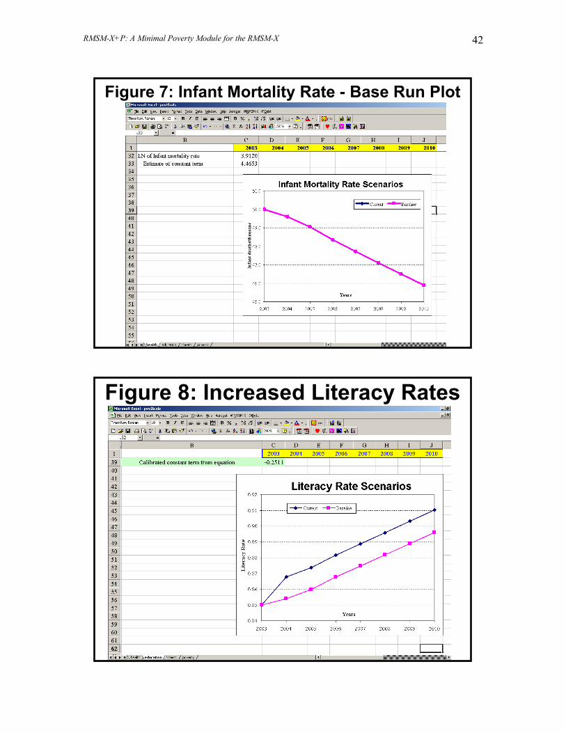
RMSM-X+P: A Minimal Poverty Module for the RMSM-X 42
Figure 7: Infant Mortality Rate - Base Run Plot
Figure 8: Increased Literacy Rates
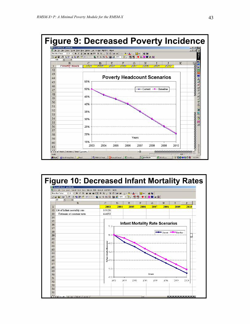
RMSM-X+P: A Minimal Poverty Module for the RMSM-X 43
Figure 9: Decreased Poverty Incidence
Figure 10: Decreased Infant Mortality Rates
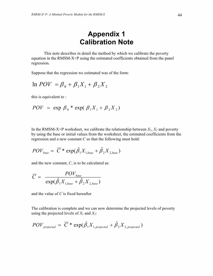
RMSM-X+P: A Minimal Poverty Module for the RMSM-X 44
Appendix 1 Calibration Note
This note describes in detail the method by which we calibrate the poverty
equation in the RMSM-X+P using the estimated coefficients obtained from the panel regression. Suppose that the regression we estimated was of the form:
22110ln XXPOV βββ ++= this is equivalent to :
)exp(*exp 22110 XXPOV βββ += In the RMSM-X+P worksheet, we calibrate the relationship between X1, X2 and poverty by using the base or initial values from the worksheet, the estimated coefficients from the regression and a new constant C so that the following must hold:
)ˆˆexp(* ,22,11 basebasebase XXCPOV ββ += and the new constant, C, is to be calculated as:
)ˆˆexp( ,22,11 basebase
base
XXPOVC
ββ +=
and the value of C is fixed hereafter The calibration is complete and we can now determine the projected levels of poverty using the projected levels of X1 and X2:
)ˆˆexp(* ,22,11 projectedprojectedprojected XXCPOV ββ +=
RMSM-X+P: A Minimal Poverty Module for the RMSM-X 45
Appendix 2 Poverty Module formulae and
External links to the Poverty Module Macroeconomic Projections: GDP deflator: directly feeds from Derived Indicators Table (DIT) sheet of the Macroeconomic Module of RMSM-X (row 112 in the DIT sheet of standard RMSM-X); Government expenditures as a share of GDP: directly feeds from Deriver Indicators Table (DIT) sheet of the Macroeconomic Module of RMSM-X (row 137 in the DIT sheet of standard RMSM-X); Education expenditures as a share of GDP: calculated as a product of Government expenditures as a share of GDP from RMSM-X (as described above) and the assumed share of education expenditures in total public expenditures (row 20 of education sheet of the Poverty module); GDP per capita (constant LCU): calculated as a ratio of total real GDP per capita in local currency and mid-year available population, both directly fed from the Macroeconomic Module of RMSM-X: total GDP per capita – from the System of National Accounts (SNA) sheet (row 46 in the SNA sheet of standard RMSM-X), and mid-year population – from Prices, Interest, Tariffs (PIT) sheet (row 3 in the PIT sheet of standard RMSM-X). Real growth of GDP per capita: calculated from the GDP per capita (constant LCU) series obtained as described above; Openness: calculated as a sum of exports and imports of goods and services from Deriver Indicators Table (DIT) sheet of the Macroeconomic Module of RMSM-X (rows 39 and 40 in the DIT sheet of standard RMSM-X); Poverty Projections: Calibration of constant term: The constant term for the chosen base year is calculated using base year values for the poverty headcount, logarithm of GDP per capita (constant LCU), real growth of GDP per capita, logarithm of economic openness, logarithm of Gini coefficient and the specified elasticities from estimated equations. Poverty level projection: The direct calculation of the headcount indicator is reported in the relevant line in the poverty module sheet. A step-by-step calculation of the relevant equation is provided for checking purposes.
RMSM-X+P: A Minimal Poverty Module for the RMSM-X 46
Charts: For the poverty-related indicators calculated in the worksheet, corresponding charts are provided. These enable the comparison of the current scenarios against a “baseline” scenario, which is obtained by “freezing” any chosen scenario, changing relevant assumptions and comparing the results. For this purpose, a toolbar has been provided with a button linked to an Excel worksheet “macro”. If the toolbar is not visible, use Excel’s view facility to show the toolbar called “pov”. To set any chosen scenario as the “baseline”, click on the toolbar button, which shows a smiling yellow face. Then, change any given assumption and press “F9” to recalculate the results and check the charts to see the impacts of the changes made to assumptions. Alternatively, the same result can be achieved by running the worksheet macro called “pov” and then changing any assumptions as desired.
Related Documents


