THE RELATIVE STRENGTH OF ABIOTIC AND BIOTIC …

THE RELATIVE STRENGTH OF ABIOTIC AND BIOTIC CONTROLS ON SPECIES RANGE

LIMITS

by

ALLISON LOUTHAN

B.A., Grinnell College, 2008

A thesis submitted to the

Faculty of the Graduate School of the

University of Colorado in partial fulfillment

of the requirement for the degree of

Doctor of Philosophy

Environmental Studies Program

2016

This thesis entitled: The Relative Strength of Abiotic and Biotic Controls on Species Range Limits

written by Allison Marie Louthan has been approved for the Environmental Studies Program

Daniel Doak

Sharon Collinge

Brett Melbourne

Date

The final copy of this thesis has been examined by the signatories, and we find that both the content and the form meet acceptable presentation standards

of scholarly work in the above mentioned discipline.

iii

ABSTRACT

Louthan, Allison Marie (Ph.D., Environmental Studies Program)

The Relative Strength of Abiotic and Biotic Controls on Species Range Limits

Thesis directed by Professor Daniel F. Doak

Study of the determinants of species’ geographic distributions has a rich tradition in ecology and

evolution, and understanding these determinants is becoming increasingly important in the face

of climate change. While we know many range limits are set by abiotic stress, species

interactions can also be important drivers of range limits. However, we lack any well-tested

predictive framework for when and where each of these two broad classes of factors will most

commonly set range limits.

A long-standing, but still nearly untested, hypothesis suggests that abiotic stress most

often sets range limits in seemingly stressful areas, such as arctic, high-alpine, or arid systems,

with species interactions having more influence in apparently benign environments, such as the

tropics, low-elevation, or mesic places. In my dissertation, I experimentally tested a fundamental

assumption of this hypothesis: namely, that the relative importance of species interactions and

abiotic stress for population performance varies systematically with abiotic stress. I tested the

relative importance of abiotic stress vs. three species interactions (herbivory, neighbors, and

pollinators) for population dynamics of a model plant species in central Kenya, Hibiscus meyeri,

across a sharp aridity gradient.

I find broad-scale support for Darwin’s hypothesis, with stronger effects of herbivores,

neighbors, and pollinators on population growth rate in mesic areas v. arid areas. Interestingly, I

find universal competitive effects of neighbors (rather than the switch from facilitative to

iv

competitive with increasing rainfall predicted by recent theoretical and empirical work). This

work suggests that species interactions might be critical drivers of range limits only in

unstressful regions of a species range.

This work also has implications for projecting shifts in species’ distributions. While in

some cases, leaving biotic interactions out of species’ distribution models reduces accuracy, the

vast majority of projections of shifts in distributions with climate change do not include such

interactions. This work suggests that species distribution modelers should include species

interactions in their predictions only in abiotically benign portions of a species range.

v

DEDICATION

In memory of Antony Eschwa.

vi

ACKNOWLEDGEMENTS

I would like to thank the invaluable help I have received from my advisor, Daniel Doak, as well

as from my committee members and the Principal Investigators of UHURU. I am also grateful

for funding from the P.E.O. Scholar Award, The University of Colorado-Boulder, the L’Oréal-

UNESCO Award for Women in Science, the American Philosophical Society (Lewis and Clark

Fund), a Doctoral Dissertation Improvement Grant, NSF DEB-1311394, NSF DEB-0812824 to

D. Doak, the University of Wyoming, the Wyoming NASA Space Grant, and the Bureau of Land

Management.

vii

CONTENTS

CHAPTER I. INTRODUCTION .................................................................................... 1 Purpose of the Study ........................................................................... 2 Experimental Design of the Study ...................................................... 3 Arrangement of the Thesis ................................................................. 4 II. WHERE AND WHEN DO SPECIES INTERACTIONS SET RANGE LIMITS? ................................................................ 6 Abiotic and Biotic Determinants of Species Ranges .................... 7 A Brief History of Range Limit Theory ....................................... 9 Tests of the Forces Governing Range Limits ............................. 10 A Clear Definition of SIASH ..................................................... 12 Possible Mechanisms Determining Species Interaction Strength across Stress Gradients ........................................... 15 Concluding Remarks and Future Directions .............................. 21 Supporting Details ...................................................................... 24 III. CLIMATIC STRESS MEDIATES THE IMPACTS OF HERBIVORY ON PLANT POPULATION STRUCTURE AND COMPONENTS OF INDIVIDUAL FITNESS .................................................................. 30 Introduction ................................................................................ 31 Materials and Methods ............................................................... 34 Results ........................................................................................ 40 Discussion ................................................................................... 47

viii

IV. MECHANISMS OF PLANT-PLANT INTERACTIONS: CONCEALMENT FROM HERBIVORES IS MORE IMPORTANT THAN ABIOTIC-STRESS MEDIATION IN AN AFRICAN SAVANNAH ....................................................................... 54 Introduction ................................................................................ 55 Materials and Methods ............................................................... 57 Results ........................................................................................ 64 Discussion ................................................................................... 68 V. SPECIES INTERACTIONS MORE STRONGLY AFFECT POPULATION GROWTH RATE IN UNSTRESSFUL AREAS ......... 73 Introduction ................................................................................ 74 Results and Discussion ............................................................... 76 Materials and Methods ............................................................... 82 VI. CONCLUSION ...................................................................................... 88 Summary of consistent patterns .................................................. 89 Future work ................................................................................. 90 BIBLIOGRAPHY……………………..…………………………………………Error! Bookmark not defined. APPENDIX A. CHAPTER 2 APPENDIX .................................................................... 111 B. CHAPTER 3 APPENDIX .................................................................... 112 C. CHAPTER 4 APPENDIX .................................................................... 121 D. CHAPTER 5 APPENDIX .................................................................... 126 E. PERMISSIONS TO USE PUBLISHED MANUSCRIPTS ................. 139

ix

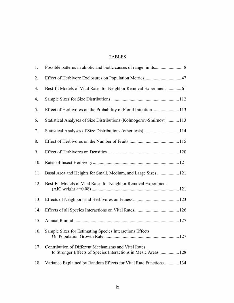
TABLES 1. Possible patterns in abiotic and biotic causes of range limits ......................... 8 2. Effect of Herbivore Exclosures on Population Metrics ................................ 47 3. Best-fit Models of Vital Rates for Neighbor Removal Experiment ............. 61 4. Sample Sizes for Size Distributions ........................................................... 112 5. Effect of Herbivores on the Probability of Floral Initiation ....................... 113 6. Statistical Analyses of Size Distributions (Kolmogorov-Smirnov) .......... 113 7. Statistical Analyses of Size Distributions (other tests) ............................... 114 8. Effect of Herbivores on the Number of Fruits ............................................ 115 9. Effect of Herbivores on Densities .............................................................. 120 10. Rates of Insect Herbivory ........................................................................... 121 11. Basal Area and Heights for Small, Medium, and Large Sizes ................... 121 12. Best-Fit Models of Vital Rates for Neighbor Removal Experiment (AIC weight >=0.08) ............................................................................ 121 13. Effects of Neighbors and Herbivores on Fitness ........................................ 123 14. Effects of all Species Interactions on Vital Rates ....................................... 126 15. Annual Rainfall ........................................................................................... 127 16. Sample Sizes for Estimating Species Interactions Effects On Population Growth Rate ................................................................. 127 17. Contribution of Different Mechanisms and Vital Rates to Stronger Effects of Species Interactions in Mesic Areas ................. 128 18. Variance Explained by Random Effects for Vital Rate Functions ............. 134

x

19. Effect of Species Interactions and Rainfall on Population Growth Rate .................................................................. 136

FIGURES

1. A Functional Definition of Species Interactions- Abiotic Stress Hypothesis ....................................................................... 14

2. Four Mechanisms Dictating the Strength of Species Interactions ............................................................................................. 16 3. A Priori Support for SIASH is Mixed .......................................................... 19

4. The Effect of Herbivore Exclosures on the Probability of Initiating Reproduction .......................................................................................... 41 5. The Effect of Herbivore Exclosures on Fruits Per Biomass ........................ 41 6. The Effect of Herbivore Exclosures on Size Distributions ......................... 42 7. The Effect of Herbivore Exclosures on Basal Area Density ....................... 44 8. Differential Effects of Herbivore Exclosures on Size Distributions .................................................................................. 45 9. The Effect of Herbivores and Neighbors on Growth and Fitness ................ 65 10. Loss of Support for the Stress Gradient Hypothesis with Increasing Herbivore Activity ................................................................ 67 11. The Effect of Species Interactions on Population Growth Rate ................... 77 12. Effect of Rain and Species Interactions on Vital Rates ................................ 78 13. Decomposition of Mechanisms Generating Stronger Effects of Species Interactions in Mesic Areas ....................................................... 80 14. Schematic of UHURU ................................................................................ 116 15. Empirical CDFs of Size Distributions ........................................................ 117 16. Effect of Herbivores on Height: Basal Area Ratio ..................................... 118 17. Effect of Herbivores on Gini Coefficients .................................................. 119

xi

18. Effect of Neighbors and Herbivores on Survival and Reproduction ........................................................................................ 124 19. Effect of Neighbors and Herbivores on Growth (Raw Data) ..................... 125 20. Effect of Species Interactions on Population Growth Rate without Block Effects and with Non-Specific Predictors ..................... 129 21. Sensitivities of Population Growth Rate .................................................... 130 22. Selfing Rates ............................................................................................... 132 23. Measurement Error ..................................................................................... 134

1

CHAPTER 1

INTRODUCTION The ecology of species’ geographic distributions, including range limits and abundance

patterns, has long fascinated ecologists (Darwin 1859), and is becoming increasingly urgent to

understand given accelerating climate change. While we know that both abiotic stress and

species interactions can set species distributions (Sexton et al. 2009), projections of changes in

species’ distributions with climate change still largely rely on the assumption that distributions

are determined only by abiotic stress, such as freezing or aridity tolerance. In contrast, ecologists

have historically predicted that abiotic stress is of primary importance only at some range edges

(e.g., northern and high elevation range limits) with geographic limits in apparently more benign

locations (southern and low-elevation limits) more strongly controlled by biotic factors, such as

parasite load, predation pressure, or herbivory (Darwin 1859, MacArthur 1972, May &

MacArthur 1972). This long-standing hypothesis predicts that the strength of species interactions

in shaping population growth and persistence will shift systematically with increasing abiotic

stress. Determining which of these assumptions or hypotheses is more correct is critical in

understanding applied issues such as climate change, as well as fundamental biogeographic

patterns.

Despite the fact that ecologists have often suggested that abiotic stress may be a more

critical driver of population dynamics in apparently harsher habitats, and biotic factors more

influential in abiotically benign environments (Darwin 1859, May & MacArthur 1972, Gross &

Price 2000, Grace et al. 2002, Harley 2003), we lack strong empirical evidence supporting this

claim (see Chapter 2). Connell’s (1961b) classic studies provide perhaps the best support for this

2

hypothesis: in his work, intertidal species’ distributions were constrained by abiotic stress in

harsh environments and by competition with conspecifics and predation in benign environments.

In addition, subsequent work has shown differential effects of interspecific competition,

pollinator limitation, and herbivory on individual plant performance across stress gradients

(Callaway et al. 2002, Chase et al. 2000, Bingham & Ort 1998). However, many of these studies,

including Connell’s, address stress gradients at extremely local, rather than geographic scales. In

addition, to date, the effects of multiple species interactions have not been combined into a

cohesive framework that addresses their relative importance for populations at different levels of

abiotic stress. Addressing these multiple effects requires a common demographic modeling

framework that explicitly incorporates numerous causal factors, allowing simultaneous analysis

of the strength of multiple biotic and abiotic stressors (Caswell 2001, Morris & Doak 2002,

Palmer et al. 2010).

My dissertation directly addresses this issue, using experimental approaches to gauge the

importance of multiple species interactions (both positive and negative) across stress gradients,

thus allowing explicit predictions about how species interactions and climatic stress interact to

determine population persistence, abundance, and, ultimately, species’ distributions. To construct

these predictions, I study the population level effects of herbivory (a negative interaction that

decreases fitness), pollination (a positive interaction that increases fitness), and inter-plant

interactions (which may shift in sign from negative to positive with increasing stress: Callaway

et al. 2002) for a single, model plant species, Hibiscus meyeri, across a sharp aridity gradient in

an arid sub-Saharan savanna community in East Africa. In this precipitation-driven system, water

availability is one of the major gradients in abiotic stress and is thought to strongly influence

plant distributions. Traditional theory suggests that population dynamics should be controlled

3

primarily by water stress in arid areas, but by species interactions in more mesic sites. Since

largely natural communities of both large and small herbivores and their predators still persist in

my study area, this system is uniquely suited to explore the relative strength of multiple biotic

factors and climatic stress in a relatively intact ecosystem.

A unique benefit of a demographic approach is the ability to distinguish the demographic

mechanisms driving responses to species interactions. In particular, studying individual plant

responses to a range of manipulated and quantified species interactions allows me to tease apart

three distinct but often confounded mechanisms by which the strength of biotic effects can

change across stress gradients: (A) changes in the ratio of number of plants to interactors (e.g. a

higher number of herbivores per plant in mesic areas); (B) alterations in the strength of the per

capita effect of a given interactor on a plant (e.g., if plants in arid areas are better defended, each

herbivore may remove smaller amounts of tissue per plant); or (C) changes in the sensitivity of

population growth to an interaction (e.g., lower seedling germination in arid areas reduces the

elasticity of population growth to herbivores’ reduction of fruit number). My work will

distinguish among these different scenarios, thus isolating the effect of aridity on pollinator,

herbivore, or neighboring plant population densities from its alterations of life history patterns

and hence effects of interactors.

In addition, my focus on aridity as an abiotic stressor is unusual. Predictions about the

relative importance of biotic interactions apply to all gradients of abiotic stress, but have largely

been invoked for latitudinal or elevational patterns in performance, often thought to mainly result

from temperature. In contrast, little work has focused on aridity gradients, though we know

precipitation patterns will change drastically with climate change and that these changes will

result in as great or greater disruption in ecosystems than will warming alone (IPCC Climate

4

Change 2007, Crimmins et al. 2011). Further, aridity is one of the most pervasive forms of

abiotic stress, with 40% of the world’s landmass classified as arid or semi-arid, according to the

UNCCD classification system, and nearly 40% of the world’s human population living in these

areas (White & Nackoney 2003). Aridity is also known to strongly control plant performance

and abundance, and is predicted to change drastically with future climate change (Covey et al.

2003). In arid areas, we need to know when and where biotic interactions are critical drivers of

individual species’ population dynamics, both to anticipate range shifts in natural areas, and to

correctly manage controllable interactions, such as cattle grazing, that could either exacerbate or

help ameliorate climate-driven shifts in species and community distributions.

In addition to providing a framework for assessing the relative strength of different

drivers on population performance, and an empirical test of a long-standing theory on the origins

and maintenance of range limits, my dissertation also has direct implications for accurately

predicting shifts in species distributions with climate change. Although we know species

interactions can be critical drivers of population health and species’ distributions (Brown 1971,

Gotelli et al. 2010, Jankowski et al. 2010, Sexton et al. 2009), faithfully incorporating them into

distribution models is a formidable challenge. As noted above, most “climate envelope” or

species distribution modeling approaches implicitly assume that species’ distributions are

primarily a function of abiotic variables (e.g. temperature and precipitation) and the biotic factors

that directly covary with these abiotic variables. Thus, this work will serve to illuminate where

and when species interactions should be included in species distribution models, and where and

when abiotic variables alone can be used to accurately predict shifts in species range limits.

Together, the following chapters seek to cover the range of topics just outlined. Chapter 2

provides a theoretical and empirical background for the hypotheses of differential mechanisms

5

for range limitation, including predictions for when and where species interactions might be most

common and why. This chapter has been published as: Louthan AM, Doak DF, Angert, AL.

2015. Where and When do Species Interactions Set Range Limits? Trends in Ecology &

Evolution 30, 780-792. Chapter 3 addresses the population-level effects of herbivores on H.

meyeri; this chapter has been published as: Louthan AM, Doak DF, Goheen JR, Palmer TM,

Pringle RM. 2013. Climatic stress mediates the impacts of herbivory on plant population

structure and components of individual fitness. Journal of Ecology 101, 1074-1083. Chapter 4

presents results on the fitness consequences of neighboring plants and how these effects interact

with herbivory. This chapter has been published as: Louthan AM, Doak DF, Goheen JR, Palmer

TM, Pringle RM. 2014 Mechanisms of plant – plant interactions: concealment from herbivores is

more important than abiotic-stress mediation in an African savannah. Proc. R. Soc. B 281:

20132647. In Chapter 5, I synthesize all of these data to show at what level of aridity species

interactions exert stronger effects on H. meyeri population performance and why. Finally, a brief

concluding chapter summarizes my overall findings.

6

CHAPTER 2

WHERE AND WHEN DO SPECIES INTERACTIONS SET RANGE LIMITS? Used with permission from Louthan AM, Doak DF, Angert, AL, Where and When do Species

Interactions Set Range Limits?, Trends in Ecology & Evolution, 30, 780-792, Elsevier, 2015. See

Appendix.

Abstract

A long-standing theory, originating with Darwin, suggests that abiotic forces set species range

limits at high latitude, high elevation, and other abiotically ‘stressful’ areas, while species

interactions set range limits in apparently more benign regions. This theory is of considerable

importance for both basic and applied ecology, and while it is often assumed to be a ubiquitous

pattern, it has not been clearly defined or broadly tested. We review tests of this idea and dissect

how the strength of species interactions must vary across stress gradients to generate the

predicted pattern. We conclude by suggesting approaches to better test this theory, which will

deepen our understanding of the forces that determine species ranges and govern responses to

climate change.

Trends

Both climate and species interactions set species range limits, but it is unclear when each

is most important.

An old hypothesis, first proposed by Darwin, suggests that abiotic factors should be key

drivers of limits in abiotically stressful areas, and species interactions should dominate in

abiotically benign areas.

7

Four distinct mechanisms, ranging from per-capita effects to community-level synergies,

could result in differential importance of species interactions across stress gradients.

These mechanisms, operating alone or in tandem, can result in patterns consistent or

inconsistent with Darwin's hypothesis, depending on the strength and direction of effects.

The most robust test of this hypothesis, not to date performed in any study, is to analyze

how sensitive range limit location is to changes in the strength of one or more species

interactions and also to abiotic stressors.

Abiotic and Biotic Determinants of Species Ranges

The ever-mounting evidence of continuing climate change has focused attention on

understanding the geographic ranges (see Glossary in Appendix) of species, and in particular

how these ranges might shift with changes in climate (Parmesan & Yohe 2003, Loarie et al.

2009). A major complication to these efforts, often mentioned but rarely formalized, is that all

populations occur in a milieu of other species, with multiple, often complex species interactions

affecting individual performance, population dynamics, and hence geographic ranges. The

implicit assumption of most modern work on range shifts is that either directly or indirectly,

climate is the predominant determinant of ranges, but interactions among species might also limit

species, current and future geographic ranges (Van der Putten et al. 2010, Pigot & Tobias 2013,

Wisz et al. 2013). Determining where and when climate alone creates range limits, and where

and when it is also critical to consider species interactions, will allow us to identify the most

likely forces setting species range limits.

A better understanding of the forces creating range limits is especially important for the

accurate prediction of geographic range shifts in the face of both climate change and

anthropogenic impacts on species interactions (e.g., introduction of exotic species, shifts in

8

interacting species ranges, and extinction or substantial reductions of native populations; Bois et

al. 2013, Gillson et al. 2013, Raffa et al. 2013, Ripple et al. 2014). For example, predictions of

shifts in species distributions might only need to consider direct effects of climate to be accurate,

but if species interactions also exert strong effects, we must include both climate and these more

complex effects in our predictions. Finally, if species interactions are important in some sections

of a species range but not in others, we can be adaptive in the inclusion of these effects when

formulating predictions.

We frame our discussion of the drivers of range limits around the long-standing

prediction that climate and other abiotic factors are far more important in what appear to be

abiotically stressful areas, whereas the effects of species interactions predominate in setting

range limits in apparently more benign areas; we call this the ‘Species Interactions–Abiotic

Stress Hypothesis’ (SIASH; Table 1). To clarify the evidence and possible causal mechanisms

underlying SIASH, we first summarize past work on the drivers of range limits. We then propose

a more operational statement of the hypothesis and discuss a series of different mechanisms that

could explain systematic shifts in the strength of species interactions across abiotic stress

gradients. We end by discussing ways to better test the factors setting range limits.

Cause of cold edge range limit

Cause of warm edge range limit

Pattern generated

Abiotic stress Abiotic stress Only abiotic stress determines species

distribution Species interactions Species interactions Only species interactions

determine species distribution

Abiotic stress Species interactions SIASH Species interactions Abiotic stress Opposite of SIASH

Table 1. Possible patterns in abiotic and biotic causes of range limits.

9

A Brief History of Range Limit Theory

Most early work on range limits emphasized the role of abiotic stress (e.g., von Humboldt &

Bonpland 1807, Merriam 1894; see “Causes of Range Limits, below”), but naturalists also

speculated that both abiotic stress and species interactions were important determinants of limits

(Table 1). For example, Grinnell (1917) observed that the California thrasher (Toxostoma

redivivum) range is loosely constrained to a specific climatic zone, but in the presence of another

thrasher species, it is more tightly constrained. Also, not all authors agreed that the importance of

species interactions would vary as predicted by SIASH. Griggs (1914) found that competition

sets northern range limits for some plant species, and Janzen (1967) hypothesized that the

breadth of abiotic tolerance is narrower in tropical montane species than in temperate montane

species, and thus that climate constrains species elevational ranges more tightly in the tropics.

Despite these different ideas, most thinking about the role of species interactions in range

limit formation has centered around the predictions of SIASH. As with so many ecological

concepts and theories, Darwin, in On the Origin of Species (1859), provides the first clear

articulation of the idea:

When we travel from south to north, or from a damp region to a dry, we invariably see some species gradually. . .disappearing; and the change of climate being conspicuous, we are tempted to attribute the whole effect to its direct action. But. . .each species. . .is constantly suffering enormous destruction. . .from enemies or from competitors for the same place and food. . .When we travel southward and see a species decreasing in numbers, we may feel sure that the cause lies quite as much in other species being favoured, as in this one being hurt. . .When we reach the Arctic regions, or snow-capped summits, or absolute deserts, the struggle for life is almost exclusively with the elements. (Darwin 1859, Chapter 3, p. 66)

Dobzhansky (1950) MacArthur (1972) and Brown (1995) all emphasized geographic patterns

arising from SIASH, suggesting that low-latitude range limits are set by species interactions

10

(most commonly negative interactions such as competition or predation) and higher-latitude

limits by abiotic stressors.

Tests of the Forces Governing Range Limits

A plethora of correlational studies suggest a major role for abiotic stress in setting range limits

(see references in Gaston 2003), but direct effects of abiotic stress on physiological performance

or fitness in the context of range limits have been more difficult to document (Sexton et al. 2009;

we also note that species find many different conditions ‘stressful’).

There is also abundant evidence that species interactions, both negative and positive (e.g.,

facilitation or pollination), can and do influence species ranges. In addition to modeling work

(e.g., Case et al. 2005), Sexton et al. (2009) found that the majority of empirical studies looking

for biotic determinants of range limits found support for these effects. Most commonly, studies

addressing biotic determinants of range limits show correlations between density of a focal

species and that of their competitors or predators (e.g., Bullock et al. 2000), or attribute a lack of

demonstrable abiotic control over nonstressful or trailing range limits to biotic factors (Ettinger

et al. 2011, Sunday et al. 2012). Competition, predator– prey dynamics, or hybridization can all

constrain occurrence patterns of species (Anderson et al. 2002, Aragón & Sánchez-Fernández

2013, Pigot & Tobias 2013, Tingley et al. 2014), while mutualisms can extend ranges (Afkhami

et al. 2014). However, little work measures effects of biotic factors on demographic or

extinction–colonization processes (See “Causes of Range Limits”; but see Pennings & Silliman

2005, Kauffman & Maron 2006), and fewer still connect such fine-scale information to

geographic range limits (but see Stanton-Geddes et al. 2012).

It is even more difficult to quantify the fraction of range limits set by abiotic versus biotic

factors, or when and where abiotic versus biotic factors will dominate, much less why such

11

patterns might arise. Doing so is primarily limited by a lack of studies that address both abiotic

and biotic determinants of species ranges in the same system. Nonetheless, studies in several

ecological systems allow provisional tests of SIASH, although often with a lack of connection

between work on local processes and large-scale patterns. At the fine scale, Kunstler et al. (2011)

show that tree growth is more reduced by competitors in areas with greater water availability and

temperature. Conversely, for an annual plant along a moisture gradient, Moeller et al. (2012)

show that plant reproduction is more limited by pollinator service in stressful than in benign

locations. There are also many large-scale studies suggestive of SIASH: in conifers, abiotic

stress more often limits growth at high elevations, while other factors, presumably species

interactions, are more important at low-elevation limits (Ettinger et al. 2011, but see Ettinger &

HilleRisLambers 2013, which finds no variation in the strength of competition across

elevations), and similar work shows correlations suggestive of SIASH in crabs (DeRivera et al.

2005) and birds (Gross & Price 2000). Stott and Loehle's work (1998) on boreal trees also

supports SIASH. In a meta-analysis of over-the-range-limit transplant experiments, Hargreaves

et al. (2014) demonstrated that fitness is often reduced beyond high latitude or high elevation

limits (consistent with limits set by abiotic stress), whereas fitness remains high beyond most

low latitude or low elevation limits (consistent with at least partial control by species

interactions). Studies of invasive species, which are often known or suspected of having reduced

enemies or competitors in their introduced range, show mixed results. In the tropics, many

invasive birds and mammals have very broad geographic ranges, suggesting that their native

ranges were tightly controlled by species interactions, consistent with SIASH. However, outside

the tropics, most high-latitude invasive species have larger range sizes than extratropical lower-

12

latitude invasive species, inconsistent with SIASH (Sax 2001). Importantly, a minority of these

studies use experimental manipulations (Moeller et al. 2012, Hargreaves et al. 2014).

The rocky intertidal offers the best work on the mechanisms settings range limits at both

large and small scales. These systems offer clear local stress gradients and harbor many

experimentally tractable species, with low adult mobility and clear-cut range limits; all of the

studies cited below use experimental manipulations. At the fine-scale, Connell (1961b) found

support for SIASH: predation and competition more strongly affect population density in the

lower intertidal, which is less abiotically stressful than the upper intertidal. Subsequent work

found similar patterns for these and other interactions, including predation (Paine 1974, but see

Wootton 1993, one of multiple studies showing large effects of predation by birds in the upper

intertidal), competition (Wethey 1984, Wethey 2002), and herbivory (Harley 2003; but see

Underwood 1980, where herbivores prevent establishment of algae in the upper intertidal). At

the macroecological scale, Sanford et al. (2003) found support for SIASH, with increased

frequency of predation on the mussel Mytilus californianus in low latitudes (see also Paine 1966,

Freestone et al. 2011). Wethey (1983, 2002) has shown that for intertidal barnacles, high-latitude

limits are set by competition and low-latitude limits by temperature intolerance, a pattern

conforming to the prediction of SIASH regarding abiotic stress, but not the common latitudinal

pattern in range limits that assumes stress is lowest in the tropics.

A Clear Definition of SIASH

Although there is an extensive literature on the causes of range limits, and ecologists often

assume that SIASH is a strong generality (e.g., Connell 1961b, Ettinger et al. 2011, Hargreaves

et al. 2014), a clear operational definition of the hypothesis is lacking. Many of the studies

discussed above show evidence that one or more performance measures are differentially

13

affected by biotic or abiotic forces, but not evidence concerning their influence on range limits or

expansion or population growth at range margins. An added complication is that ‘stress’ is

extremely difficult to define or manipulate (e.g., Helmuth et al. 2006, Crimmins et al. 2011),

since multiple conditions can be stressful, many species are known to find both ends of an

abiotic gradient stressful (e.g., thermal neutral zones of endotherms and physiological activity

ranges of ecotherms), and many abiotic stressors are negatively correlated (e.g., drought stress

and freezing stress along an elevational gradient). Before delving further into how the patterns

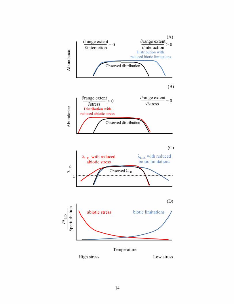
predicted by SIASH could arise, we therefore suggest this definition: ‘amelioration of biotic

limits to growth would expand the range much more at the nonstressful than the stressful end of

some gradient in abiotic conditions, and conversely for amelioration of abiotic stress’. This

definition also has a corollary about the forces governing local population growth at range limits:

low density stochastic growth rate (λL.D.) of local populations is predicted to be more strongly

influenced by species interactions at the nonstressful end of an abiotic gradient, and by abiotic

forces near to the stressful end; because population presence or extinction are functions of

population growth at low densities, controls on performance under these conditions are the

critical metric of effects on range limits. This definition emphasizes the dual pattern that SIASH

predicts, has a clear graphical interpretation (Fig. 1), and also can be analyzed using standard

demographic methods (See “Formulating Demographic Tests of SIASH”). We also know of no

studies that quantify response of range-limit growth rate to different drivers while accounting for

density to arrive at estimates of low-density growth rate.

14

Abu

ndan

ce

Abu

ndan

ce

λ L.D

.

!1!

Temperature

(A)

(B)

(C)

(D)

High stress Low stress

∂range extent ∂stress > 0

∂λL.

D.!

∂p

ertu

rbat

ion

∂range extent ∂interaction = 0

∂range extent ∂interaction > 0

Observed distribution

Distribution with reduced biotic limitations

Observed distribution

Distribution with reduced abiotic stress

abiotic stress biotic limitations

Observed λL.D.

λL.D. with reduced biotic limitations

λL.D. with reduced abiotic stress

∂range extent ∂stress = 0

15

Figure 1. A Functional Definition of Species Interactions–Abiotic Stress Hypothesis (SIASH) Patterns and Predictions. SIASH predicts that the sensitivity of range extent to species interactions (∂range extent/∂interaction) is high at the nonstressful end of a species range. At the nonstressful end, species interactions drive local abundances to zero (i.e., set the range limit), so that release from these limitations (blue line) would lead to significant, stable expansion from the observed distribution (black line). (B) Conversely, SIASH predicts that sensitivity of range extent to stress (∂range extent/ ∂stress) is high at the stressful end of a species range, such that release from these limitations (red line) will result in stable range expansion from the observed distribution (black line). (C) While conducting experiments to measure actual range expansion is generally difficult (Connell's experimental work on barnacles, 1961b, is perhaps the best example of such a study), under realistic assumptions, sensitivities of low-density population growth rate (λL.D.) mirror sensitivities of range extent, such that alleviation of biotic limitations or stress results in range expansion (species is extant where λL.D.≥ 1; colors as in A and B). (D) SIASH can be tested by assessing the sensitivity of λL.D. to perturbations in both species interactions and abiotic stress (∂λL.D./ ∂perturbation; red is sensitivity to abiotic stress and blue to biotic limitations).

Possible Mechanisms Determining Species Interaction Strength across Stress Gradients

It is evident (and perhaps even tautological) that abiotic stress will be limiting in places that are

abiotically stressful. The less obvious aspect of SIASH is why species interactions should be

weak in stressful areas and strong in abiotically benign areas. Understanding if these patterns

hold is therefore a key part of testing the generality of SIASH. There are a number of aspects or

levels of species interactions, not all of which necessarily lead to SIASH, but few statements of

the theory are specific about what component of species interactions are alleged to change across

stress gradients. For example, SIASH predicts that parasitism should exert stronger effects on

range limits in less stressful areas. However, one might predict that where stress is high, there

should be larger effects of a given parasite load on host performance because of decreased ability

to recover from infection. Where stress is low, conversely, there might be weaker effects of that

same parasite load due to increased reproductive rates that compensate for negative effects of

parasites. In this scenario, we would actually expect that parasitism will have larger effects in

stressful places, contrary to the predictions of SIASH. To further complicate matters, variation in

16

parasite load, parasite infection rate, and parasite species diversity will also influence the net

effect of the interaction.

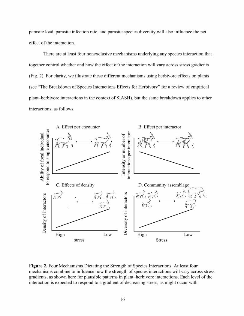
There are at least four nonexclusive mechanisms underlying any species interaction that

together control whether and how the effect of the interaction will vary across stress gradients

(Fig. 2). For clarity, we illustrate these different mechanisms using herbivore effects on plants

(see “The Breakdown of Species Interactions Effects for Herbivory” for a review of empirical

plant–herbivore interactions in the context of SIASH), but the same breakdown applies to other

interactions, as follows.

Figure 2. Four Mechanisms Dictating the Strength of Species Interactions. At least four mechanisms combine to influence how the strength of species interactions will vary across stress gradients, as shown here for plausible patterns in plant–herbivore interactions. Each level of the interaction is expected to respond to a gradient of decreasing stress, as might occur with

Div

ersi

ty o

f int

erac

tors

Den

sity

of i

nter

acto

rs

Abi

lity

of fo

cal i

ndiv

idua

l to

resp

ond

to si

ngle

enc

ount

er

In

tens

ity o

r num

ber o

f in

tera

ctio

ns p

er in

tera

ctor

High Low stress

High Low Stress

A. Effect per encounter B. Effect per interactor

C. Effects of density D. Community assemblage

17

increasing temperature, rainfall, or nutrient availability. Inset pictographs illustrate these mechanisms for interactions between a focal food plant and its gazelle herbivore. (A) Effect per encounter. The impact of a single feeding bout on the fitness of an individual plant, with increased plant regrowth following herbivory in low-stress areas. (B) Effect per interactor. Cumulative effects of a lifetime of interactions between one gazelle and one plant, with higher consumption, and hence impact, in high-stress areas. (C) Effects of density. The effect of a population of gazelle on the population of a focal plant, with higher gazelle-to-plant ratio in low-stress areas. (D) Community assemblage. Effects of a guild of interactors on a plant population, with greater diversity of herbivore species in low-stress areas. The direction of each mechanism across a stress gradient might be positive or negative, and will not necessarily conform to the pattern shown in these panels (see text for more details).

Mechanism 1: Effect per Encounter

The demographic effect of each interspecific encounter (e.g., one bite from one herbivore)

changes across stress gradients, such that focal individuals respond differentially to an encounter

as a function of abiotic stress level. For example, the ability of an individual plant to maintain λ

= 1 following one feeding bout by one herbivore appears likely to decrease as stress increases

(Fig. 2), opposing SIASH.

Mechanism 2: Effect per Interactor

The effect of an individual interactor on a focal individual (e.g., the effect of one herbivore on

one plant over their lifetimes) varies across stress gradients. For example, colder conditions are

likely to mean greater energetic needs for endothermic herbivores and hence higher feeding rates

(Fig. 2); this would contradict SIASH. Alternatively, a generalist herbivore might feed on a

variety of plant species in stressful, low-primary-productivity environments, but specialize on a

focal plant species in nonstressful, high-productivity environments; this could support SIASH.

Mechanism 3: Effects of Density

The ratio of the population densities of two species changes across stress gradients, such that

population-level effects of the interaction vary. For example, herbivore-to-plant ratios might

18

increase with increasing temperature or rainfall, supporting SIASH (Fig. 2), or show the opposite

pattern, contradicting SIASH.

Mechanism 4: Community Assemblage

Finally, the richness or diversity of species within a guild changes across stress gradients, with

resulting changes in the limitations imposed on species the guild interacts with. For example, a

plant suffering more types of damage from a richer herbivore community might be more strongly

impacted than one living with a less diverse set of consumers (Fig. 2). If herbivore communities

are richer in low-stress areas than in high-stress areas, this would support SIASH.

The most fundamental difference among the above mechanisms is between effects

generated by the interactions between pairs of individuals (mechanisms 1 and 2) versus effects

generated by the populations and communities of interacting species (mechanisms 3 and 4). The

original proponents of SIASH (Darwin 1859, Dobzhansky 1950, MacArthur 1972, Brown 1995)

emphasized that gradients in interactor density or richness, mechanisms 3 and 4, are common

along gradients in abiotic stress. Similarly, Menge and Sutherland's formulation of this

hypothesis (1987) relies on increased food web complexity in nonstressful areas. A recent review

by Schemske et al. (2009) suggests that, concomitant with the well-known decreases in species

richness with latitude, the frequency of many types of species interactions also decrease with

latitude for a wide variety of species. We might predict that increases in interactor density and

species richness with decreasing stress (and by extension, increased number and diversity of

interactions) might make SIASH very common in nature. However, variation in interaction

strength (mechanisms 1 or 2) could strongly influence this conclusion. For example, if a prey's

risk of capture increases with stress (mechanism 1), but, simultaneously, predator density

decreases with stress (mechanism 3), the net effect of predation might not vary. Similarly, if

19

predators require more food in stressful areas to maintain body condition (mechanism 2), but

predator density decreases with stress (mechanism 3), the net effect of predation might vary in

either direction. Different combinations of these mechanisms can generate an overall pattern

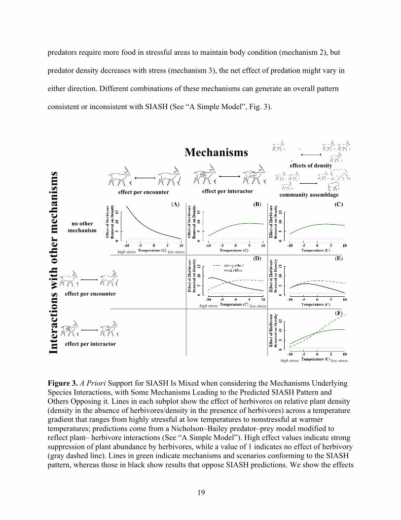
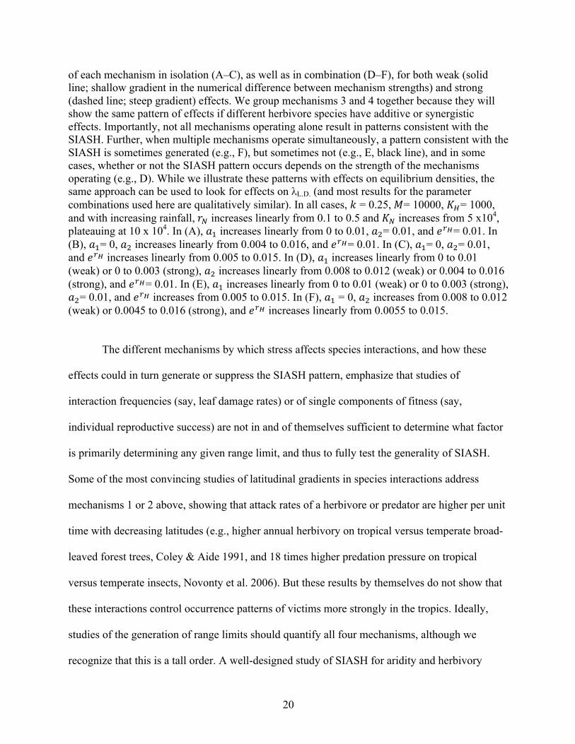
consistent or inconsistent with SIASH (See “A Simple Model”, Fig. 3).

Figure 3. A Priori Support for SIASH Is Mixed when considering the Mechanisms Underlying Species Interactions, with Some Mechanisms Leading to the Predicted SIASH Pattern and Others Opposing it. Lines in each subplot show the effect of herbivores on relative plant density (density in the absence of herbivores/density in the presence of herbivores) across a temperature gradient that ranges from highly stressful at low temperatures to nonstressful at warmer temperatures; predictions come from a Nicholson–Bailey predator–prey model modified to reflect plant– herbivore interactions (See “A Simple Model”). High effect values indicate strong suppression of plant abundance by herbivores, while a value of 1 indicates no effect of herbivory (gray dashed line). Lines in green indicate mechanisms and scenarios conforming to the SIASH pattern, whereas those in black show results that oppose SIASH predictions. We show the effects

effect per encounter

effect per interactor

no other mechanism

Inte

ract

ions

with

oth

er m

echa

nism

s

effect per encounter effect per interactor community assemblage

effects of density

Mechanisms

high stress low stress

high stress low stress

high stress low stress

20

of each mechanism in isolation (A–C), as well as in combination (D–F), for both weak (solid line; shallow gradient in the numerical difference between mechanism strengths) and strong (dashed line; steep gradient) effects. We group mechanisms 3 and 4 together because they will show the same pattern of effects if different herbivore species have additive or synergistic effects. Importantly, not all mechanisms operating alone result in patterns consistent with the SIASH. Further, when multiple mechanisms operate simultaneously, a pattern consistent with the SIASH is sometimes generated (e.g., F), but sometimes not (e.g., E, black line), and in some cases, whether or not the SIASH pattern occurs depends on the strength of the mechanisms operating (e.g., D). While we illustrate these patterns with effects on equilibrium densities, the same approach can be used to look for effects on λL.D. (and most results for the parameter combinations used here are qualitatively similar). In all cases, 𝑘 = 0.25,  𝑀= 10000, 𝐾!= 1000, and with increasing rainfall,  𝑟! increases linearly from 0.1 to 0.5 and 𝐾! increases from 5 x104, plateauing at 10 x 104. In (A), 𝑎! increases linearly from 0 to 0.01, 𝑎!= 0.01, and 𝑒!!= 0.01. In (B), 𝑎!= 0, 𝑎! increases linearly from 0.004 to 0.016, and 𝑒!!= 0.01. In (C), 𝑎!= 0, 𝑎!= 0.01, and 𝑒!! increases linearly from 0.005 to 0.015. In (D), 𝑎! increases linearly from 0 to 0.01 (weak) or 0 to 0.003 (strong), 𝑎! increases linearly from 0.008 to 0.012 (weak) or 0.004 to 0.016 (strong), and 𝑒!!= 0.01. In (E), 𝑎! increases linearly from 0 to 0.01 (weak) or 0 to 0.003 (strong), 𝑎!= 0.01, and 𝑒!! increases from 0.005 to 0.015. In (F), 𝑎! = 0, 𝑎! increases from 0.008 to 0.012 (weak) or 0.0045 to 0.016 (strong), and 𝑒!! increases linearly from 0.0055 to 0.015.

The different mechanisms by which stress affects species interactions, and how these

effects could in turn generate or suppress the SIASH pattern, emphasize that studies of

interaction frequencies (say, leaf damage rates) or of single components of fitness (say,

individual reproductive success) are not in and of themselves sufficient to determine what factor

is primarily determining any given range limit, and thus to fully test the generality of SIASH.

Some of the most convincing studies of latitudinal gradients in species interactions address

mechanisms 1 or 2 above, showing that attack rates of a herbivore or predator are higher per unit

time with decreasing latitudes (e.g., higher annual herbivory on tropical versus temperate broad-

leaved forest trees, Coley & Aide 1991, and 18 times higher predation pressure on tropical

versus temperate insects, Novonty et al. 2006). But these results by themselves do not show that

these interactions control occurrence patterns of victims more strongly in the tropics. Ideally,

studies of the generation of range limits should quantify all four mechanisms, although we

recognize that this is a tall order. A well-designed study of SIASH for aridity and herbivory

21

might assess sensitivity of λL.D. to rainfall and herbivore density at range limits and conduct over-

the-range-limit transplants with and without supplemental watering treatments and herbivore

exclosures (“Formulating Demographic Tests of SIASH”). Support for or against SIASH might

arise due to any of the four mechanisms detailed above.

Concluding Remarks and Future Directions

Understanding why range limits are where they are, and predicting how climate change, species

losses, and other global changes will alter them are key questions in applied and basic ecology.

While SIASH is a long-standing hypothesis, there are still few thorough tests of its predictions.

Whether or not SIASH provides a strong generality depends on the relative strength of different

mechanisms that will combine to create or negate patterns in the importance of abiotic versus

biotic limitations to population persistence (Fig. 3). However, we currently lack empirical tests

of the underlying processes or exact predictions of the hypothesis that would be needed to judge

support for SIASH (see “Outstanding Questions”).

We see three avenues to increase our understanding of when and where SIASH is a

useful generality. First, field studies that quantify the strength of each of the four interaction

mechanisms affecting population growth rate could be used to parameterize simple models (e.g.,

“A Simple Model”) to assess support for SIASH. Such work could use relatively simple

experiments replicated across broad-scale geographic gradients to fill in information in already

well-studied systems (Maron et al. 2014).

A second need is for studies of how demographic processes vary with stress, or multiple

stressors, across a species range, and thus the effect of stress in limiting low-density population

growth rates. For example, if seedling germination is already limited by abiotic determinants of

safe site abundance, reduction of plant fecundity by herbivores might have muted effects on

22

plant abundance; conversely, if recruitment is not safe site-limited, reduction of fecundity by

herbivores will have large population-level effects (Maron et al. 2014). Few studies address

variation in vital rates and sensitivity of population growth rate to those vital rates across broad

geographic ranges (but see Angert 2009, Doak & Morris 2010, Eckhart et al. 2011, Villellas et

al. 2012), and even fewer quantify the factors driving variation in these rates (e.g., Doak &

Morris 2010, Fisichelli, Frelich & Reich 2012), Stanton-Geddes et al. 2012) or consider density

effects.

Finally, even if the predictions of SIASH are supported, there are very few studies that

directly address whether simple reductions in local population performance are usually the key

factor limiting ranges (“Causes of Range Limits”), (Angert 2009, Doak & Morris 2010, Eckhart

et al. 2011). In particular, we have little empirical evidence showing how metapopulation

dynamics affect range limits (Fukaya et al. 2014). In addition, it is unclear if small-scale

determinants of species range limits at the local scale are governed by mechanisms similar to

determinants that operate at geographic scales. Thus, studies trying to address determinants of

range limits should clearly articulate the scale of their work relative to the range of the study

species (e.g., Emery et al. 2012).

Predicting where and when the inclusion of species interactions will meaningfully

improve range limit predictions is critical to predicting the ecological consequences of climate

change (Guisan & Thuiller 2005, Angert et al. 2013), but we have evidence that there is wide

variation in how important these species interactions are (Godsoe et al. 2015). Focusing on the

relative importance of different factors in driving ranges and their dynamics are particularly

important because species might shift their ranges idiosyncratically with climate, resulting in

novel communities, and because many climate change-caused extinction events have been

23

suggested to arise via altered species interactions, rather than climate shifts per se (Harley 2011,

Cahill et al. 2013, Tunney et al. 2014). While the predictions of SIASH might or might not prove

robust to empirical tests, the four mechanisms underlying SIASH provide a framework for

testing the most likely forces setting species range limits in a variety of systems and thus could

help us more accurately predict shifts in geographic ranges.

Outstanding Questions

Do abiotic stress or species interactions have a strong influence on species range limits? Whereas

there is ample evidence from the literature that both abiotic stress and species interactions can set

limits, some species limits may be caused by dispersal limitation, or ranges may not be at

equilibrium. Thus, we encourage ecologists to devote substantial time to observing causes of

reduced performance at range limits, and assessing whether abiotic and biotic factors are likely

drivers, before quantifying their influence on population growth.

What is the effect of both abiotic and biotic forces on fitness or population growth? Many

existing studies quantify responses of only one fitness component to abiotic or biotic forces, but

not overall population growth, especially at low densities, and hence range limits.

What is the total effect of a given species interaction across abiotic gradients, considering

potentially different trends at multiple levels of the interaction, including individual responses, as

well as density and community assemblage effects? The four mechanisms we outline here are a

starting point to consider effects at multiple levels; measuring the strength of poorly studied

mechanisms in well-studied systems that have already measured some mechanisms could be

especially productive.

24

How do different demographic processes vary with abiotic stress? We have a poor

understanding of how abiotic stress affects vital rates for many species, and thus a limited ability

to predict how species interactions will influence population growth.

Are reductions in local population performance or metapopulation persistence the key

driver of range limits? Conducting more studies comparing these two forces would both increase

our ability to predict whether SIASH is a strong generality, as well as further our understanding

of all species range limits and geographic shifts in those limits with climate change.

Causes of Range Limits

In addition to simple dispersal limitation, three demographic processes can set range limits (Holt

& Keitt 2000, Holt et al. 2005): (i) a reduction of average deterministic growth rate such that a

population can no longer be established or survive; (ii) increased variability in demographic

rates, such that stochastic growth rates are too low for establishment or persistence (Boyce et al.

2006); and (iii) increasingly patchy habitat distributions or lower equilibrium local population

sizes, so that extinction–colonization dynamics will no longer support a viable metapopulation.

For simplicity, we emphasize declines in mean performance in our presentation, but both of the

other processes can also enforce range limits, through similarly interacting effects of species

interactions and abiotic variables on demographic rates. Both empirical and modeling work

suggest that all of these demographic processes can operate in nature, but this breakdown of

demographic causes of range limits is agnostic with respect to underlying abiotic or biotic

drivers.

Anywhere a species is extant, we expect that, over the long term, populations are able to

grow from small numbers to some stable population density (although not necessarily the same

density everywhere), but the demographic reasons that this condition is not met – and hence a

25

range limit is hit – can vary geographically. For example, survival rates could decline at high

temperatures, while reproduction fails at low temperatures, such that population growth rates are

higher at intermediate temperatures, but fall at both extremes. Similarly, different abiotic

stressors might simultaneously vary over a single geographic gradient: at high elevations cold

can reduce survival, while at low elevations, drought can do the same (e.g., Morin et al. 2007: for

aspen, drought is stressful in southern populations, but cold is stressful in northern populations).

In contrast to these examples, the classic assumption behind SIASH, and most tests of SIASH, is

that abiotic stress gradients are one dimensional and monotonic in their effects on population

growth, either increasing or decreasing along a latitudinal or elevational gradient. SIASH also

assumes that each range limit arises either from abiotic or biotic factors, while it is quite likely

that many range limits result from strong synergies between abiotic and biotic factors, rather than

just one class of factors alone.

Formulating Demographic Tests of SIASH

SIASH is sometimes phrased in a way that denies contradiction: a range limit at the stressful end

of an abiotic gradient is determined by stress, and the range limit at the other, nonstressful end of

the gradient is determined by something else (species interactions), because there is no abiotic

stress there. Stress gradients are also often assumed to follow what humans might see as stressful

versus nonstressful conditions. However, both ends of even a simple abiotic gradient can pose

difficulties for a species, and many stress gradients are nonlinear or polytonic. Finally, range

limits can be determined by multiple, interacting factors, with biotic and abiotic factors exerting

some control over population performance across a species range.

Given these difficulties, the most robust test of SIASH is analyzing how sensitive range

limit location is to changes in the strength of one or more species interactions (in the currency of

26

any of the four mechanisms we outline) versus abiotic stressors. SIASH predicts that the

sensitivity of range limit expansion to the alleviation of a biotic limitation (reduction of a

negative interaction or increase in a positive one) will be much greater at the low-stress end of a

geographic range than the other, with a converse sensitivity to abiotic stress alleviation (Fig. 1)

over the long term.

SIASH could be tested using across-range-limit transplants combined with manipulations

of abiotic and abiotic factors. However, such experiments can be difficult, must be conducted

over fairly long time periods, and are sometimes inadvisable ethically. An alternative is to

evaluate whether λL.D. values of populations at low-stress range limits have greater sensitivity to

experimental reduction of biotic limitations than do λL.D. values at high-stress limits (and,

whether sensitivity to abiotic stress shows the converse pattern). Low-density growth rates,

which determine probability of population establishment or extinction, will best correlate with

population presence and persistence even if range limit populations are at high density (Birch

1953). In established populations, short-term focal individual manipulations (e.g., local density

reductions) can be used to estimate λL.D.. Assuming that this sensitivity is a continuous function

of abiotic conditions and such conditions change continuously across range limits, sensitivity of

λL.D. to abiotic or biotic factors should mirror the sensitivity of range limitation (Fig. 1).

Discontinuities in either abiotic stressors or species interactions across range limits will

obviously complicate the interpretation of this measure of range limitation sensitivity.

The Breakdown of Species Interactions Effects for Herbivory

Studies of herbivory, a particularly well-studied set of species interactions, help illustrate how

the direction and strength of the four mechanisms can differ along a stress gradient. The

Compensatory Continuum Hypothesis (CCH) predicts that stressed plants are less able to

27

compensate for herbivore damage (mechanism 1, Maschinski & Whitman 1989; although Hilbert

et al. 1981 predict the opposite, also see Hawkes & Sullivan 2001). Relevant to mechanism 2,

herbivore metabolic rate, and thus food intake, is also often higher in thermally stressful areas

(Dunbar & Brigham 2010, Dell et al. 2011), but the opposite is true for precipitation (Scheck

1982, Soobramoney et al. 2003). Supporting our illustration of mechanisms 3 and 4, herbivore

densities, herbivore/plant ratios, and herbivore species richness are generally higher in dense

plant stands and nonstressful areas (Root 1973, McNaughton et al. 1989, Rosenzweig 1995,

Ritchie & Olff 1999, Forkner & Hunter 2000, Jones et al. 2011, Salazar & Marquis 2012).

Some studies of herbivory also quantify the relative strength of multiple mechanisms.

Pennings et al. (2009) found very high herbivory rates on low latitude salt marsh plants,

consistent with SIASH, resulting from a combination of higher herbivore feeding rates

(mechanism 2) and much higher herbivore densities (mechanism 3) in low latitudes than in high

latitudes (but high herbivore densities have also been shown to drastically impact salt marsh

plants in the high arctic; Handa et al. 2002). However, differences in the strength and direction of

these very same mechanisms can lead to net effects inconsistent with SIASH: in Piper plants,

herbivore densities are highest at the equator, but lower herbivore feeding rates in these same

areas (possibility due to higher plant defenses) mean that herbivory rates do not differ with

latitude (Salazar & Marquis 2012).

Different mechanisms can also exert strong feedback on one another, further complicating

efforts to predict when we expect to see SIASH-like patterns. Miller et al. (2009) showed that

cactus (Opuntia imbricata) herbivores were most abundant at low elevations (mechanism 3); in

turn, this high herbivore pressure acted to reduce cactus densities, thus increasing per-capita

effect of herbivores (mechanism 2) due to lack of food. These examples serve to illustrate that

28

mechanisms can exacerbate or nullify one another and, that in some cases, the pattern generated

by multiple mechanisms is extremely difficult to predict using only limited data on single

mechanisms.

A Simple Model

We use a simple heuristic model of plant response to herbivory to show how the four

mechanisms composing a species interaction could contribute to the generation of range limits.

We simplify herbivory, the only species interaction in this example, to a simple consumptive

effect that results in an immediate reduction in plant size and growth. We use this model to

explore how different mechanisms contribute to the sum effect of herbivory on plant populations

across a temperature gradient.

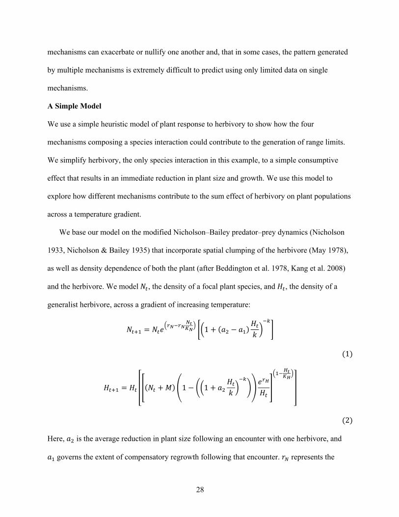
We base our model on the modified Nicholson–Bailey predator–prey dynamics (Nicholson

1933, Nicholson & Bailey 1935) that incorporate spatial clumping of the herbivore (May 1978),

as well as density dependence of both the plant (after Beddington et al. 1978, Kang et al. 2008)

and the herbivore. We model  𝑁!, the density of a focal plant species, and 𝐻!, the density of a

generalist herbivore, across a gradient of increasing temperature:

𝑁!!! = 𝑁!𝑒!!!!!

!!!! 1+ 𝑎! − 𝑎!

𝐻!𝑘

!!

(1)

𝐻!!! = 𝐻! 𝑁! +𝑀 1− 1+ 𝑎!𝐻!𝑘

!! 𝑒!!𝐻!

!!!!!!

(2)

Here, 𝑎! is the average reduction in plant size following an encounter with one herbivore, and

𝑎!  governs the extent of compensatory regrowth following that encounter. 𝑟! represents the

29

intrinsic rate of increase of the plant, 𝐾! the carrying capacity, and  𝑘 the spatial clumping of

herbivores. Analogously, 𝑟! represents the conversion rate of plants to herbivores and 𝐾!

herbivore carrying capacity; 𝑀 is the density of other food sources of herbivores. We model

mechanism 1 (effect per encounter) by increasing 𝑎!with temperature, mechanism 2 (effect per

herbivore) by increasing 𝑎! with temperature, and mechanisms 3 and 4 via increasing 𝑟! with

temperature.

We first consider each mechanism in isolation, assuming what seem to us plausible

directions for these effects with increasing temperature, and then explore combinations of

mechanisms. While effects of each mechanism in isolation are relatively easy to predict (Fig.

3A–C), when considering multiple mechanisms, support for SIASH is highly contingent on the

strength of individual effects (Fig. 3D–F), illustrating that the conditions under which SIASH is

supported or refuted will depend on the strength and exact pattern of each of the four

mechanisms and how they vary with stress. These results suggest that the net pattern generated

by multiple mechanisms is impossible to predict in the absence of quantitative data on the

relative strength of different mechanisms. No empirical study to our knowledge measures the

strength of all of these mechanisms for any one species or type of interaction.

Acknowledgments

We would like to thank members of the Doak laboratory, J. Maron, and A. Hargreaves for

helpful comments. Support for this work came from CU-Boulder, the P.E.O. Scholar Award, the

L’Oréal–UNESCO Award for Women in Science, and NSF 1311394 to A.M.L., NSF 1242355,

1340024 and 1353781 to D.F.D, and NSF 0950171 and Natural Sciences and Engineering

Research Council of Canada to A.L.A.

30

CHAPTER 3

CLIMATIC STRESS MEDIATES THE IMPACTS OF HERBVIORY ON PLANT POPULATION STRUCTURE AND COMPONENTS OF INDIVIDUAL FITNESS

Published as: Louthan AM, Doak DF, Goheen JR, Palmer TM, Pringle RM. 2013. Climatic

stress mediates the impacts of herbivory on plant population structure and components of

individual fitness. Journal of Ecology 101, 1074-1083.

Summary

Past studies have shown that the strength of top-down herbivore control on plant physiological

performance, abundance and distribution patterns can shift with abiotic stress, but it is still

unclear whether herbivores generally exert stronger effects on plants in stressful or in

nonstressful environments. One hypothesis suggests that herbivores’ effects on plant biomass

and fitness should be strongest in stressful areas, because stressed plants are less able to

compensate for herbivore damage. Alternatively, herbivores may reduce plant biomass and

fitness more substantially in nonstressful areas, either because plant growth rates in the absence

of herbivory are higher and/or because herbivores are more abundant and diverse in nonstressful

areas. We test these predictions of where herbivores should exert stronger effects by measuring

individual performance, population size structure and densities of a common subshrub, Hibiscus

meyeri, in a large-scale herbivore exclosure experiment arrayed across an aridity gradient in East

Africa. We find support for both predictions, with herbivores exerting stronger effects on

individual-level performance in arid (stressful) areas, but exerting stronger effects on population

size structure and abundance in mesic (nonstressful) areas. We suggest that this discrepancy

arises from higher potential growth rates in mesic areas, where alleviation of herbivory leads to

31

substantially more growth and thus large changes in population size structure. Differences in

herbivore abundance do not appear to contribute to our results. Synthesis: Our work suggests that

understanding the multiple facets of plant response to herbivores (e.g. both individual

performance and abundance) may be necessary to predict how plant species’ abundance and

distribution patterns will shift in response to changing climate and herbivore numbers.

Introduction

Where, when and how top-down forces are important in structuring populations and

communities is an enduring topic in ecology. Trophic interactions such as predation and

herbivory affect primary productivity and species composition in a variety of systems, both

through direct reductions in prey or producer biomass (e.g. Estes & Palmisan 1974; McNaughton

1985; Olff & Ritchie 1998), as well as via indirect effects mediated through prey risk perception

or through plant and prey establishment patterns (e.g. Schmitz 2005; Riginos & Young 2007).

While much of the literature on top-down control focuses on trophic cascades, with effects of

predators transmitted through herbivores to primary producers, we also know that climatic and

other abiotic factors affect the strength of herbivore control of plant productivity and

performance. However, most of this work has been conducted in artificial settings or via

simulated herbivory, and most studies have addressed herbivores’ effects on individual

performance. Here, we ask whether climate influences the degree to which herbivory shapes both

individual plant performance and population structure using a large-scale exclosure experiment

arrayed across a natural rainfall gradient in an East African savanna.

Herbivores affect plant communities in a variety of ways, including consumption of

biomass, suppression of competitively dominant or highly palatable species, and alteration of

habitat structure (Olff & Ritchie 1998). Although we know that the strength of these effects can

32

be contingent on abiotic context (Maschinski & Whitham 1989; Anderson et al. 2007; Pringle et

al. 2007; Schmitz 2008), results from past studies on the relative direction and magnitude of

herbivore effects on plant abundance and composition across stress gradients have been

inconsistent. Some studies show that herbivores have weaker effects on plant biomass in areas of

lower stress (Chase et al. 2000), but, conversely, denser and more diverse herbivore communities

(Cyr & Pace 1993) or higher plant growth rates in lower-stress areas may result in stronger

herbivore suppression of potential plant biomass in these sites. Similarly, while most studies find

that herbivores exert stronger effects on community composition in less stressful areas (e.g.

Chase et al. 2000; Bakker et al. 2006), others show that herbivores alter plant species

composition most markedly in areas of intermediate or even low rainfall (Anderson et al. 2007).

The apparent inconsistency of these results stems in part from a poor understanding of how the

relatively well-studied individual-level responses to herbivory translate into changes in

population abundance and structure across stress gradients at a broader scale (Anderson & Frank

2003). This lack of knowledge limits our ability to predict how variation in abiotic stress and

herbivory regimes will drive shifts in plant populations and communities.

From past work, three hypotheses about how herbivores affect plants across abiotic stress

gradients generate competing predictions; we call these the ‘Compensatory Continuum Model’

(following Maschinski & Whitham 1989), the ‘Herbivore Pressure Hypothesis’ and the

‘Differential Growth Rate Hypothesis.’ The Compensatory Continuum Model predicts that in

less productive areas, plants will suffer a reduced ability to compensate for herbivory (e.g.

Josefsson 1970; Louda & Collinge 1992; Joern & Mole 2005), and the combination of stress and

herbivory will therefore generate synergistic effects that strongly reduce plant performance and

abundance. In more productive areas, plants can better tolerate and/or compensate for the effects

33

of herbivory (e.g. via plant regrowth or sustained recruitment of new individuals following

herbivory), and thus, the impacts of herbivory on plant biomass should be low (White 1984). In

contrast, the Herbivore Pressure and Differential Growth Rate Hypotheses predict that herbivores

exert stronger effects on biomass in less stressful areas. This phenomenon occurs either because

herbivores are generally more abundant and diverse in less stressful areas (Cyr & Pace 1993,

here called the Herbivore Pressure Hypothesis) or because in less stressful areas, potential plant

growth in the absence of herbivory is high (Differential Growth Rate Hypothesis). Both of these

hypotheses predict that the difference between plant populations with and without herbivores

(e.g. individual-, population- and community-level biomass) should be greater in less stressful

areas.

Most studies of herbivory effects concentrate on one of two scales: individual plant

responses or changes in abundance or biomass at the population level. For example, the

Compensatory Continuum model is usually measured at the individual scale, whereas the

Herbivore Pressure and Differential Growth Rate Hypotheses are often tested at the population

level. Between these two extremes are herbivore effects on the population structure of plants

(size, shape or age distribution), which reflect how the responses of individual plants manifest as

population-wide effects (Staudhammer & LeMay 2001; Rubin et al. 2006; Drewa et al. 2008;

Prior et al. 2011). These distributions provide a straightforward way to capture information on

the cumulative effects of herbivory and abiotic stress on populations (Prior et al. 2011), averaged

over many years of variation in these factors. This approach is particularly valuable for assessing

the long-term effects of herbivores, whose population densities – and thus their effects on plants

– can be quite variable from year to year. Thus, examining the consequences of herbivory for

34

population structure is a promising approach with which to augment our understanding of where

and how herbivores are important drivers of plant population dynamics.

Here, we examine how herbivory by large mammals affects several aspects of (i)

individual performance and (ii) population structure in a common East African savanna plant

(the subshrub Hibiscus meyeri) using large-scale herbivore exclosures replicated across an

abiotic stress gradient of variable rainfall. To assess support for each of the three nonexclusive

hypotheses outlined above at both the individual and population scale, we conducted short-term

measurements of growth and reproductive rates, and also characterized patterns of population

densities and size structures to measure population-wide effects of herbivory and aridity.

Materials and methods

Our study was conducted at the Mpala Research Centre, in the Laikipia District of central Kenya

(0°18′ N, 37°54′ E). Rainfall in this semi-arid acacia-dominated savanna falls in a weekly bi- or

tri-modal pattern, with little seasonality in temperature. Large common herbivores include

elephant (Loxodonta africana), giraffe (Giraffa camelopardalis), eland (Taurotragus oryx),

buffalo (Syncerus caffer), zebra (Equus quagga), waterbuck (Kobus ellipsiprymnus), impala

(Aepyceros melampus), warthog (Phacochoerus africanus) and dik-dik (Madoqua guentheri).

Elephant, impala and dik-dik attain the greatest biomass densities (2882, 813 and 693 kg km-2,

respectively), with zebra a distant fourth at 263 kg km-2 (Augustine 2010).

We assessed the effect of herbivores and climate using a largescale herbivore exclusion

experiment (Ungulate Herbivory Under Rainfall Uncertainty: ‘UHURU’) established in

September 2008 (Goheen et al. 2013). One of four treatments in UHURU is to 1-ha plots in a

randomized block design using different configurations of electric fencing: LMH treatments

exclude all Large Mammalian Herbivores (> 5 kg); MESO treatments allow dik-diks but exclude

35

mega- and mesoherbivores (> 40 kg); MEGA treatments exclude only megaherbivores

(elephants and giraffes); and Control treatments are unfenced, allowing access by all native

herbivores. Each treatment is replicated three times at each of three sites (arid, intermediate and

mesic) across a 22-km rainfall gradient (Appendix Fig. 1). Total rainfall increases > 45% from

the Arid to Mesic site (440 mm/year at the Arid site, 580 mm/year at the Intermediate site and

640 mm /year at the Mesic site). Indirect measures of herbivore activity (quarterly dung counts)

show little variation across this gradient. Only two large mammalian herbivores (impala and

zebra) show variation in densities across the gradient; impala dung density is significantly

greater at the Arid than Intermediate and Mesic sites, and zebra dung density is greater at the

Arid than Intermediate sites, neither of which differ significantly from Mesic (Goheen et al.

2013). Major soil texture and nutrient characteristics do not differ systematically across the

gradient, although the Intermediate site has lower pH than the Arid and Mesic sites (Goheen et

al. 2013). The Intermediate site also suffers from a history of overgrazing (M. Littlewood, Mpala

Ranch, pers. comm.).

Hibiscus meyeri is a short-lived subshrub present in all treatment x site combinations in

UHURU. Hibiscus meyeri’s distribution is extremely patchy, and in the presence of herbivores, it

typically occurs near or beneath trees. While some Hibiscus species produce extrafloral nectar to

attract ants that deter floral herbivores (e.g. Sugiura et al. 2006), and many species produce leaf

trichomes, presumably to deter insect herbivores, little is known about H. meyeri’s chemical

defences, and it is heavily browsed by a variety of mammalian herbivores (A. Louthan, pers.

obs.). Plant height can be substantially reduced by herbivory, and compensatory regrowth

following browsing is common, with regrowth generally occurring from extant lateral meristems

below the damaged apical meristem. Thus, stem diameter at ground level augments height to

36

provide a more reliable and stable measure of past plant size and growth. While individuals are

often single stemmed, repeated herbivory events result in a multi-stemmed phenotype that is also

common. Together, summed basal area(s) and height provide a good estimate of dry above-

ground plant biomass (adjusted r2 = 0.92, n = 39). Flowering can occur throughout the year in

response to both low- and high-volume rainfall events; fruits mature c.1 month after pollination.

Data collection: We conducted several small-scale experiments and observations to test whether

aridity is a strong driver of performance. To test that differences in performance at the Arid and

Mesic sites were driven by rainfall rather than site-specific effects, we watered 12 plants (six at

Arid site and six at Mesic site) once with 4.5 L of water during the height of a dry season in

January 2012 and, after 17–18 days, compared their performance to an unmanipulated control

group using log ratios of post vs. pretreatment fruit number. Additionally, in July 2010, we

collected one to three fruits from 47 haphazardly chosen plants (n = 22 and 25 at the Arid and

Mesic sites, respectively) and counted the nonaborted, nonpredated seeds within each fruit.

Finally, in August 2010, we simulated herbivory on 21 plants of varying sizes at the Arid and

Mesic sites by removing all leaves and reproductive organs. Two months later, we measured

regrowth of floral buds relative to the original number of buds and compared their performance

using ln[(final number of reproductive organs +1)/(initial number of reproductive organs +1)].

We tested for interacting effects of aridity and herbivory by quantifying plant

reproductive performance and population size structure at the UHURU sites over a 10-week

period in May-August 2011, c. 3 years after the exclosures were built. At each site, we searched

all treatments consecutively within one of the three blocks, moving to the next site only after the

block in the previous site was completely searched, to ensure that any phenologically driven

variability in individual performance or population structure would be confined to among-block

37

effects in our analyses. To facilitate searching and mapping, we divided each plot into fourths;

we then conducted independent searches for H. meyeri plants > 30 cm tall within each

subsection. Searches within each subsection involved scanning sequential 4-m2 areas in a

consistent predetermined pattern, censusing all plants within each 4-m2 area. We terminated our

search when we found at least four plants in a subsection or continued until the entire subsection

had been searched. We measured and mapped each plant and searched for seedlings in a 2 m

radius around all plants > 30 cm tall. At the Intermediate site, block 1 was searched during this

same period, but blocks 2 and 3 were searched over a 2-week period in January-February 2012.

We use data from these surveys to analyse population size structure.

We adopted two strategies to increase our confidence in our estimates of individual-level

effects of stress and herbivory and to investigate any artefacts arising from the UHURU

experiment. First, we increased our sample size by measuring additional, haphazardly selected

plants of varying sizes within Control and LMH treatments that were chosen as part of another

experiment (in May-August 2011, see Appendix Table 1 for sample sizes). Second, to ensure

that plants measured within Control plots in UHURU reflected the general characteristics of

plants at each site, in May-August 2011, we measured haphazardly selected plants along two 100

9 15 m belt transects within 300 m (but outside of) the UHURU Arid and Mesic sites. We used

data on height, basal area, number of fruits, number of flower buds and flowers, and probability

of reproduction from both of these sets of haphazardly selected plants to bolster samples sizes for

analyses involving these response variables. We assigned all plants measured within UHURU to

the appropriate block and treated the transect plants as a separate (fourth) block. Including these

haphazardly selected plants in our analyses of height/basal area ratio, number and probability of

reproduction had no qualitative effect on our results.

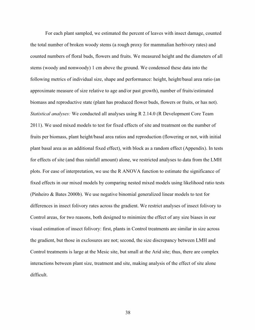
38

For each plant sampled, we estimated the percent of leaves with insect damage, counted

the total number of broken woody stems (a rough proxy for mammalian herbivory rates) and

counted numbers of floral buds, flowers and fruits. We measured height and the diameters of all

stems (woody and nonwoody) 1 cm above the ground. We condensed these data into the

following metrics of individual size, shape and performance: height, height/basal area ratio (an

approximate measure of size relative to age and/or past growth), number of fruits/estimated

biomass and reproductive state (plant has produced flower buds, flowers or fruits, or has not).

Statistical analyses: We conducted all analyses using R 2.14.0 (R Development Core Team

2011). We used mixed models to test for fixed effects of site and treatment on the number of

fruits per biomass, plant height/basal area ratios and reproduction (flowering or not, with initial

plant basal area as an additional fixed effect), with block as a random effect (Appendix). In tests

for effects of site (and thus rainfall amount) alone, we restricted analyses to data from the LMH

plots. For ease of interpretation, we use the R ANOVA function to estimate the significance of

fixed effects in our mixed models by comparing nested mixed models using likelihood ratio tests

(Pinheiro & Bates 2000b). We use negative binomial generalized linear models to test for

differences in insect folivory rates across the gradient. We restrict analyses of insect folivory to

Control areas, for two reasons, both designed to minimize the effect of any size biases in our

visual estimation of insect folivory: first, plants in Control treatments are similar in size across

the gradient, but those in exclosures are not; second, the size discrepancy between LMH and

Control treatments is large at the Mesic site, but small at the Arid site; thus, there are complex

interactions between plant size, treatment and site, making analysis of the effect of site alone

difficult.

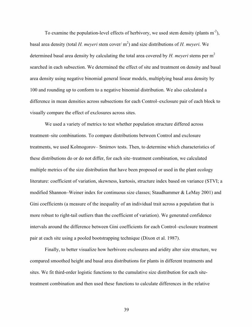
39

To examine the population-level effects of herbivory, we used stem density (plants m-2),

basal area density (total H. meyeri stem cover/ m2) and size distributions of H. meyeri. We

determined basal area density by calculating the total area covered by H. meyeri stems per m2

searched in each subsection. We determined the effect of site and treatment on density and basal

area density using negative binomial general linear models, multiplying basal area density by

100 and rounding up to conform to a negative binomial distribution. We also calculated a

difference in mean densities across subsections for each Control–exclosure pair of each block to

visually compare the effect of exclosures across sites.

We used a variety of metrics to test whether population structure differed across

treatment–site combinations. To compare distributions between Control and exclosure

treatments, we used Kolmogorov– Smirnov tests. Then, to determine which characteristics of

these distributions do or do not differ, for each site–treatment combination, we calculated

multiple metrics of the size distribution that have been proposed or used in the plant ecology

literature: coefficient of variation, skewness, kurtosis, structure index based on variance (STVI; a

modified Shannon–Weiner index for continuous size classes; Staudhammer & LeMay 2001) and

Gini coefficients (a measure of the inequality of an individual trait across a population that is

more robust to right-tail outliers than the coefficient of variation). We generated confidence

intervals around the difference between Gini coefficients for each Control–exclosure treatment

pair at each site using a pooled bootstrapping technique (Dixon et al. 1987).

Finally, to better visualize how herbivore exclosures and aridity alter size structure, we

compared smoothed height and basal area distributions for plants in different treatments and

sites. We fit third-order logistic functions to the cumulative size distribution for each site-

treatment combination and then used these functions to calculate differences in the relative

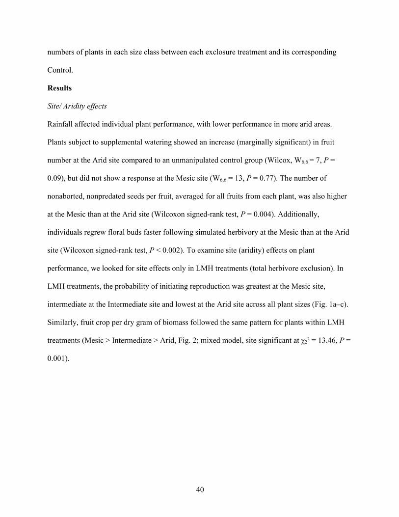
40

numbers of plants in each size class between each exclosure treatment and its corresponding

Control.

Results

Site/ Aridity effects

Rainfall affected individual plant performance, with lower performance in more arid areas.

Plants subject to supplemental watering showed an increase (marginally significant) in fruit

number at the Arid site compared to an unmanipulated control group (Wilcox, W6,6 = 7, P =

0.09), but did not show a response at the Mesic site (W6,6 = 13, P = 0.77). The number of

nonaborted, nonpredated seeds per fruit, averaged for all fruits from each plant, was also higher

at the Mesic than at the Arid site (Wilcoxon signed-rank test, P = 0.004). Additionally,

individuals regrew floral buds faster following simulated herbivory at the Mesic than at the Arid

site (Wilcoxon signed-rank test, P < 0.002). To examine site (aridity) effects on plant

performance, we looked for site effects only in LMH treatments (total herbivore exclusion). In

LMH treatments, the probability of initiating reproduction was greatest at the Mesic site,

intermediate at the Intermediate site and lowest at the Arid site across all plant sizes (Fig. 1a–c).

Similarly, fruit crop per dry gram of biomass followed the same pattern for plants within LMH

treatments (Mesic > Intermediate > Arid, Fig. 2; mixed model, site significant at χ2² = 13.46, P =

0.001).

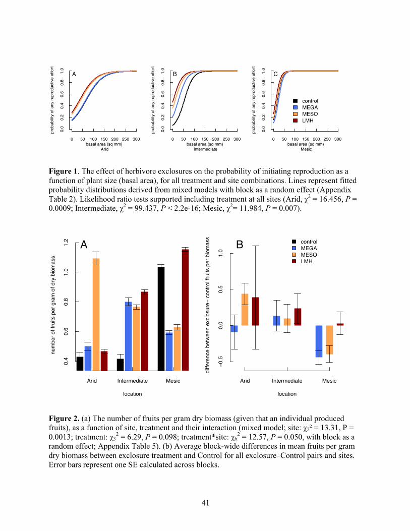
41

Figure 1. The effect of herbivore exclosures on the probability of initiating reproduction as a function of plant size (basal area), for all treatment and site combinations. Lines represent fitted probability distributions derived from mixed models with block as a random effect (Appendix Table 2). Likelihood ratio tests supported including treatment at all sites (Arid, χ2 = 16.456, P = 0.0009; Intermediate, χ2 = 99.437, P < 2.2e-16; Mesic, χ2= 11.984, P = 0.007).

Figure 2. (a) The number of fruits per gram dry biomass (given that an individual produced fruits), as a function of site, treatment and their interaction (mixed model; site: χ2² = 13.31, P = 0.0013; treatment: χ3

2 = 6.29, P = 0.098; treatment*site: χ62 = 12.57, P = 0.050, with block as a

random effect; Appendix Table 5). (b) Average block-wide differences in mean fruits per gram dry biomass between exclosure treatment and Control for all exclosure–Control pairs and sites. Error bars represent one SE calculated across blocks.

basal area (sq mm) Arid

prob

abilit

y of

any

repr

oduc

tive

effo

rt

0.0

0.2

0.4

0.6

0.8

1.0

0 50 100 150 200 250 300

A

basal area (sq mm) Intermediate

prob

abilit

y of

any

repr

oduc

tive

effo

rt

0.0

0.2

0.4

0.6

0.8

1.0

0 50 100 150 200 250 300

B

basal area (sq mm) Mesic

prob

abilit

y of

any

repr

oduc

tive

effo

rt

0.0

0.2

0.4

0.6

0.8

1.0

0 50 100 150 200 250 300

C

controlMEGAMESOLMH

location

num

ber o

f fru

its p

er g

ram

of d

ry b

iom

ass

Arid Intermediate Mesic

0.4

0.6

0.8

1.0

1.2 A

location

diffe

renc

e be

twee

n ex

clos

ure−

con

trol f

ruits

per

bio

mas

s

Arid Intermediate Mesic

−0.5

0.0

0.5

1.0

controlMEGAMESOLMH

B

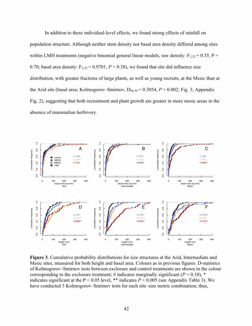
42

In addition to these individual-level effects, we found strong effects of rainfall on

population structure. Although neither stem density nor basal area density differed among sites

within LMH treatments (negative binomial general linear models, raw density: F2,32 = 0.35, P =

0.70; basal area density: F2,32 = 0.9701, P = 0.38), we found that site did influence size

distribution, with greater fractions of large plants, as well as young recruits, at the Mesic than at

the Arid site (basal area; Kolmogorov–Smirnov, D96,59 = 0.3054, P = 0.002; Fig. 3; Appendix

Fig. 2), suggesting that both recruitment and plant growth are greater in more mesic areas in the

absence of mammalian herbivory.

Figure 3. Cumulative probability distributions for size structures at the Arid, Intermediate and Mesic sites, measured for both height and basal area. Colours as in previous figures. D-statistics of Kolmogorov–Smirnov tests between exclosure and control treatments are shown in the colour corresponding to the exclosure treatment; # indicates marginally significant (P < 0.10), * indicates significant at the P < 0.05 level, ** indicates P < 0.005 (see Appendix Table 3). We have conducted 3 Kolmogorov–Smirnov tests for each site–size metric combination; thus,

basal area (sq mm)Arid

cum

ulat

ive fr

eque

ncy

●●●●●●●●●

●

●

●

●●●●●

●●●●●●●●●●●●●●●●●●●●●●

●●●●●●●●

●●●

●●●

●

0.0

0.2

0.4

0.6

0.8

1.0

0 100 200 300 400

●

●●●●●●●●

●

●●

●

●●

●●

●●●

●●●●●

●●●●●

●●●●●

●●

●●●

●●

●●

●

●●●●●

●●

●●●●●●●●●●●●●

●●●●●●●●●●●●●●●●●●●●

●●●

●●●●

●●

●●●

●●

●●

●●●

●●

●

●●●●●●●●●●●●●●●●●●●●●●●●●●●●●●●●●●●●●

●●●

●

A0.14950.2900**0.1241

controlMEGAMESOLMH

basal area (sq mm)Intermediate

cum

ulat

ive fr

eque

ncy

●●

●●

●●

●●●●●●

●

●

●●●●●●●●●●●●●●●●●●●●●●●●●●●●

●●

●●

●●

●●

B

0.0

0.2

0.4

0.6

0.8

1.0

0 100 200 300 400

●●●●●●●●●●●●●●●●●●●●●●●●●●●●●●●●●●●●●●●●●●●●●●●●●●●●●●●

●●●●

●●

●

●●●●●●●●●●●●●●●●●●●

●●●●●●●●●●●●●●●●●●●●●●●●●●●●●●●●

●●

●

●●●

●

●●●●

●●●●●●●●●●●●●●●●●●●●●●●●●●●●●●●●●●

●●●●●●●●

●●●●●●

●●

0.13030.2529*0.2638*

basal area (sq mm)Mesic

cum

ulat

ive fr

eque

ncy

●●

●●

●

●

●

●●●●

●●●●●●●●●●●●●●●●●●●●●●●●●●●●●●●●●●●●●●

●

0.0

0.2

0.4

0.6

0.8

1.0

0 100 200 300 400

●●

●

●●●●●●●●●●●●●●●●●●●●●●●●●●●●●●●●●●●●●●●●●●●●●●●●●●● ●●

●●●●●●●

● ● ● ● ● ● ● ● ●

●●●●●●●

●

●

●●●

●●●●●●●●●●●●●●●●●●●●

●●●●●●●●●●

●●

●●●●●●●●●●●

●

●●●●●●●●●●●●

●●●

●●●●●●●●●●●●●●●●●●

●●●●●●●●

● ●●●

C0.18070.20800.3966**

height (cm)Arid

cum

ulat

ive fr

eque

ncy

●●●●●●●●●●●●●●●●●●●●●●●●●●●●●●●●●●●●●●●●●●●●●●●●●●●●●●●●●●

●●●●

●●

●●●

●

D

0.0

0.2

0.4

0.6

0.8

1.0

0 100 200 300 400

●●●●●●●●●●●●●●●●●●●●●●●●●●●●●●●●●●●●●

●●●

●●●

●●●●

●●●●●●

●●

●●

●●

●

●●●●●●●●●●●●●●●●●●●●●●●●●

●●●●●●●●●●●

●●●●●●●●●●●●●●

●●●●

●●

●●

●●

●●

●●●

●●

●●

●●●●●●●●●●●●●●●●●●●●●●●●●●●●●●●●●●●●●●●●

●●●●●

●●●●●●

●●●

●●

●●●●

●●

0.14410.4131**0.2862**

height (cm)Intermediate

cum

ulat

ive fr

eque

ncy

●●●●●●●●●●●●●●●●●●●●●●●●●●●●●●●●●●●●●●●●●●●●

●●●●●●●●●●

●●

●

E

0.0

0.2

0.4

0.6

0.8

1.0

0 100 200 300 400

●●●●●●

●●●●●●●●●●●●●●●●●

●●●●●●●●

●●●●

●●●●●●●

●●●●●●

●●●

●●

●●

●●●●●

●●

●●

●●●●●●●●●●●●●●●●●●●●●●●●●●●●●●●●●●●●●●●●●●●●●●●●●

●●

●●●●

●●●

●●

●●●●●●●●●●●●●●●●●●●●●●●●●●●●●●●●●●●●●●●●●●●●●●●●●●●●●●

●●

●●●●

●●●

●●

0.2796*0.4103**0.6466**

height (cm)Mesic

cum

ulat

ive fr

eque

ncy

●●●●●●●●●●●●●●●●●●●●●●●●●●●●●●●●●●●●●●●●●●●●●●●●●●●●●●●●

●●●●●●●●●●●●●●● ● ●●

●●● ●

F

0.0

0.2

0.4

0.6

0.8

1.0

0 100 200 300 400

●●●●●●●●●●●

●●●●●●●●●●●●●●●●●●●●●●●●●●

●●●●●●

●●●●●●●●●●●●●●●●

●●●●●●●●

●●●●●●●●●●

●●●●● ●●●

● ●● ● ● ●

●●●

●●●●●●●●●●●●●●●●●●●●●●●●●●●●●●●●●●●●

●●●●●●●

●●

●●●●●●●●●

●●

●●●●●●●●●●●●●●●●●●●●●●●●●●●●●●●●●●●●●●●●●●●●●●●●●●●●●● ●● ●●

●●●●●●●●

● ●●● ●● ● ●

0.2052#0.18330.4125**

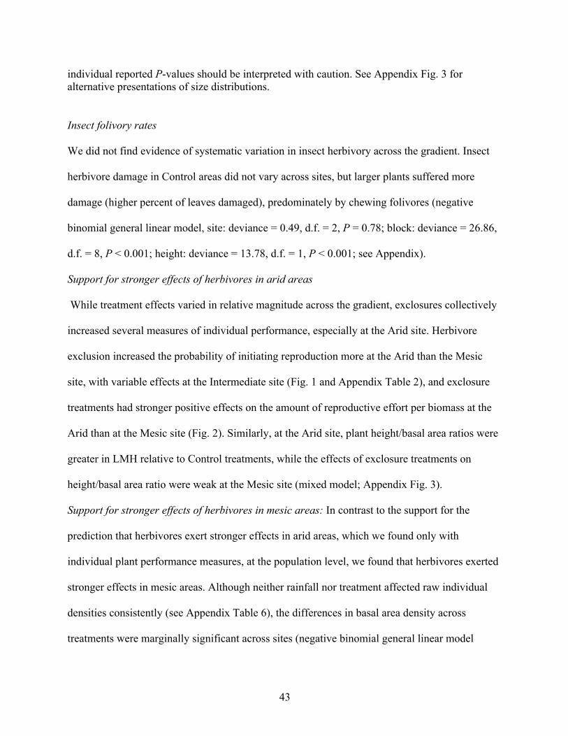
43

individual reported P-values should be interpreted with caution. See Appendix Fig. 3 for alternative presentations of size distributions.

Insect folivory rates

We did not find evidence of systematic variation in insect herbivory across the gradient. Insect

herbivore damage in Control areas did not vary across sites, but larger plants suffered more

damage (higher percent of leaves damaged), predominately by chewing folivores (negative

binomial general linear model, site: deviance = 0.49, d.f. = 2, P = 0.78; block: deviance = 26.86,

d.f. = 8, P < 0.001; height: deviance = 13.78, d.f. = 1, P < 0.001; see Appendix).

Support for stronger effects of herbivores in arid areas

While treatment effects varied in relative magnitude across the gradient, exclosures collectively

increased several measures of individual performance, especially at the Arid site. Herbivore

exclusion increased the probability of initiating reproduction more at the Arid than the Mesic

site, with variable effects at the Intermediate site (Fig. 1 and Appendix Table 2), and exclosure

treatments had stronger positive effects on the amount of reproductive effort per biomass at the

Arid than at the Mesic site (Fig. 2). Similarly, at the Arid site, plant height/basal area ratios were

greater in LMH relative to Control treatments, while the effects of exclosure treatments on

height/basal area ratio were weak at the Mesic site (mixed model; Appendix Fig. 3).

Support for stronger effects of herbivores in mesic areas: In contrast to the support for the

prediction that herbivores exert stronger effects in arid areas, which we found only with

individual plant performance measures, at the population level, we found that herbivores exerted

stronger effects in mesic areas. Although neither rainfall nor treatment affected raw individual

densities consistently (see Appendix Table 6), the differences in basal area density across

treatments were marginally significant across sites (negative binomial general linear model

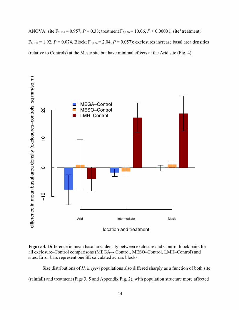
44

ANOVA: site F2,139 = 0.957, P = 0.38; treatment F3,136 = 10.06, P < 0.00001; site*treatment;

F6,130 = 1.92, P = 0.074, Block; F6,124 = 2.04, P = 0.057): exclosures increase basal area densities

(relative to Controls) at the Mesic site but have minimal effects at the Arid site (Fig. 4).

Figure 4. Difference in mean basal area density between exclosure and Control block pairs for all exclosure–Control comparisons (MEGA–- Control, MESO–Control, LMH–Control) and sites. Error bars represent one SE calculated across blocks.

Size distributions of H. meyeri populations also differed sharply as a function of both site

(rainfall) and treatment (Figs 3, 5 and Appendix Fig. 2), with population structure more affected

location and treatmentdiffe

renc

e in

mea

n ba

sal a

rea

dens

ity (e

xclo

sure

s−co

ntro

ls, s

q m

m/s

q m

)

Arid Intermediate Mesic

−10

010

20

MEGA−ControlMESO−ControlLMH−Control

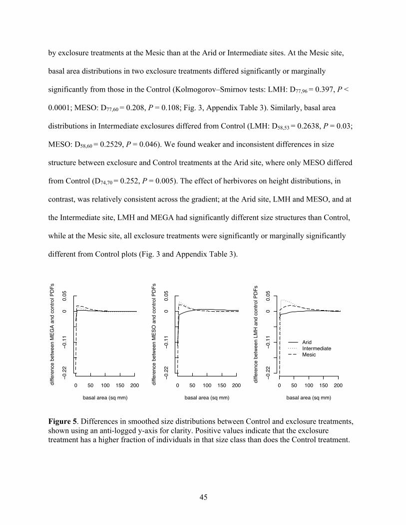
45

by exclosure treatments at the Mesic than at the Arid or Intermediate sites. At the Mesic site,

basal area distributions in two exclosure treatments differed significantly or marginally

significantly from those in the Control (Kolmogorov–Smirnov tests: LMH: D77,96 = 0.397, P <

0.0001; MESO: D77,60 = 0.208, P = 0.108; Fig. 3, Appendix Table 3). Similarly, basal area

distributions in Intermediate exclosures differed from Control (LMH: D58,53 = 0.2638, P = 0.03;

MESO: D58,60 = 0.2529, P = 0.046). We found weaker and inconsistent differences in size

structure between exclosure and Control treatments at the Arid site, where only MESO differed

from Control (D74,70 = 0.252, P = 0.005). The effect of herbivores on height distributions, in

contrast, was relatively consistent across the gradient; at the Arid site, LMH and MESO, and at

the Intermediate site, LMH and MEGA had significantly different size structures than Control,

while at the Mesic site, all exclosure treatments were significantly or marginally significantly

different from Control plots (Fig. 3 and Appendix Table 3).

Figure 5. Differences in smoothed size distributions between Control and exclosure treatments, shown using an anti-logged y-axis for clarity. Positive values indicate that the exclosure treatment has a higher fraction of individuals in that size class than does the Control treatment.

basal area (sq mm)

diffe

renc

e be

twee

n M

EGA

and

cont

rol P

DFs

−0.2

2−0

.11

00.

05

0 50 100 150 200

basal area (sq mm)

diffe

renc

e be

twee

n M

ESO

and

con

trol P

DFs

−0.2

2−0

.11

00.

05

0 50 100 150 200

basal area (sq mm)

diffe

renc

e be

twee

n LM

H a

nd c

ontro

l PD

Fs

Arid IntermediateMesic

−0.2

2−0

.11

00.

05

0 50 100 150 200

46

We found that the relative effect size of treatments varied across sites, but that LMH

treatments consistently have stronger effects on size structure in more mesic areas. To assess

which size classes were affected by exclosures at each site, we generated smoothed differences

between the plant basal area size distributions in exclosure treatments and their corresponding

Control plots. These plots (Fig. 5) indicate that the difference in size distributions between

exclosures and Control treatments is driven by consistent increases in the frequencies of small

plants at all sites, with corresponding reductions in relative numbers of medium-sized plants,

suggesting higher recruitment. These effects are strongest at the Mesic site. At both the Mesic

and Intermediate sites, these size structures suggest there was a substantial pulse of young

recruits in LMH and, at the Mesic site, the LMH treatment also increased the proportion of very

large individuals (Fig. 3). At the Arid site, in contrast, increases in small plants in the LMH

treatment were muted (Fig. 5). At the Mesic and Intermediate sites, the most extreme treatment

(LMH) had the strongest effects on size structure, but at the Arid site, MESO and MEGA had

strong effects relative to LMH.

Consistent with our analyses of full size distributions, we found weaker but similar

patterns using traditional summary metrics of size distributions. Most of these metrics showed

fairly consistent patterns across sites and supported stronger effects of herbivores at the Mesic

site. Exclosures generally increase the CV of height distributions, and the CV and kurtosis of

basal area distributions (correlated at > 0.50) at the Mesic and Intermediate sites, reflecting

greater numbers of small individuals in these areas (Table 1). We found significant differences in

Gini coefficients of height distributions in Control vs. exclosure treatments only at the Mesic site

(Appendix Fig. 4), indicating lower dispersion of size structures in exclosure treatments. For

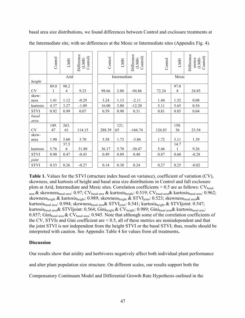
47

basal area size distributions, we found differences between Control and exclosure treatments at

the Intermediate site, with no differences at the Mesic or Intermediate sites (Appendix Fig. 4).

Con

trol

LMH

Diff

eren

ce

(LM

H-

Con

trol)

Con

trol

LMH

Diff

eren

ce

(LM

H-

Con

trol)

Con

trol

LMH

Diff

eren

ce

eren

ce

(LM

H-

Con

trol)

height Arid Intermediate Mesic

CV 89.0

1 98.2

4 9.23 98.66 3.80 -94.86 72.24 97.0

8 24.85 skew-ness 1.41 1.12 -0.29 3.24 1.13 -2.11 1.44 1.52 0.08 kurtosis 4.37 3.27 -1.09 16.00 3.80 -12.20 5.11 5.65 0.54 STVI 0.92 0.99 0.07 0.59 0.90 0.31 0.81 0.85 0.04 basal area

CV 149.47

263.61 114.15 288.39

121.65 -166.74 126.83

150.36 23.54

skew-ness 1.90 5.60 3.70 5.58 1.73 -3.86 1.72 3.11 1.39

kurtosis 5.76 37.5

6 31.80 36.17 5.70 -30.47 5.46 14.7

1 9.26 STVI 0.90 0.47 -0.43 0.49 0.89 0.40 0.87 0.60 -0.28 joint STVI 0.53 0.26 -0.27 0.14 0.38 0.24 0.27 0.25 -0.02

Table 1. Values for the STVI (structure index based on variance), coefficient of variation (CV), skewness, and kurtosis of height and basal area size distributions in Control and full exclosure plots at Arid, Intermediate and Mesic sites. Correlation coefficients > 0.5 are as follows: CVbasal

area & skewnessbasal area: 0.97; CVbasal area & kurtosisheight: 0.519; CVbasal area& kurtosisbasal area: 0.962; skewnessheight & kurtosisheight: 0.989; skewnessheight & STVIjoint: 0.523; skewnessbasal area& kurtosisbasal area: 0.994; skewnessbasal area& STVIjoint: 0.541; kurtosisheight & STVIjoint: 0.547; kurtosisbasal area& STVIjoint: 0.564; Giniheight & CVheight: 0.989; Ginibasal area& kurtosisbasal area: 0.857; Ginibasal area & CVbasal area: 0.945. Note that although some of the correlation coefficients of the CV, STVIs and Gini coefficient are < 0.5, all of these metrics are nonindependent and that the joint STVI is not independent from the height STVI or the basal STVI; thus, results should be interpreted with caution. See Appendix Table 4 for values from all treatments. Discussion Our results show that aridity and herbivores negatively affect both individual plant performance

and alter plant population size structure. On different scales, our results support both the

Compensatory Continuum Model and Differential Growth Rate Hypothesis outlined in the

48

introduction. We do not find support for the Herbivore Pressure Hypothesis; herbivore densities

are not higher in mesic areas. The effects of herbivory vary as a function of aridity, with the

strongest individual-level effects of herbivory occurring at our driest site. In contrast, herbivores

had the largest effects on population size structure at our wettest site.

Three potential mechanisms may underlie the discrepancy we observe at the individual

versus population scale. First, it is possible that there are a higher number of safe sites for

seedling establishment in mesic areas, such that smaller increases in reproductive output when

herbivores are excluded result in higher numbers of seedlings in mesic areas but not in arid areas.

However, we found no differences in total plant densities across sites, which does not support

this possibility. Second, as is true for many plant species, increases in reproductive output with

size may be nonlinear, such that relatively small increases from, for example, medium to large

size classes in mesic areas following herbivore exclusion result in substantial increases in seed

number and thus population growth – and conversely, that large absolute increases in the sizes of

(smaller) plants in arid areas result in only moderate increases in seed number and thus

population growth.

Finally, consistent with the Differential Growth Rate Hypothesis, herbivory may reduce

total plant growth more substantially in mesic areas, such that excluding herbivores results in

large effects at the Mesic site relative to dampened effects at the Arid site, giving rise to the

population-level effects we observed. Under this last scenario, the absolute potential for plant

growth in arid areas is low due to constraints imposed by aridity, even when released from

herbivory (e.g. Fig. 2). Thus, while herbivores have large individual-level effects on plant

reproduction and shape (height/ basal area ratio) in arid areas, low growth rates limit plant

response to alleviation of herbivore pressure, leading to small population-level effects, especially

49

when accumulated over time. In mesic areas, higher potential growth and reproductive rates

mean that removing herbivore pressure results in substantial increases in total growth and thus

large effects on population size structure. In support of this third hypothesis, we found that plants

at the Mesic site regrow more quickly following damage, and plants protected from herbivores

initiate reproduction at smaller sizes (Fig. 1) and produce more fruits (Fig. 2A) at the Mesic vs.

Arid or Intermediate sites. Thus, we hypothesize that herbivores exert strong effects on the

individual scale variables we measured in arid areas (supporting the Compensatory Continuum

Model), while in mesic areas, herbivores more strongly reduce potential plant growth, largely

because of reduced abiotic limitation of growth rates, supporting the Differential Growth Rate

Hypothesis at the population level.

Consistent with the predictions of the Compensatory Continuum Model, synergistic

effects of herbivory and aridity at the organismal level may result if individuals are less able to

tolerate and/or respond to damage when water stressed. A variety of studies have shown a

reduced ability to compensate for herbivore damage in the presence of abiotic stress (e.g.

Mueggler 1967; Janzen 1974; Willis et al. 1993). However, because we also observed higher

numbers of impala at the Arid site, it is unclear if higher densities of herbivores (and likely,

increased herbivory) or reduced regrowth is driving the stronger individual-level responses we

observed at the Arid site. Our study site is unusual in that we find higher densities of at least one

herbivore (impala) in arid areas, contrasting with the usual pattern of greater herbivore densities

in more mesic areas (Cyr & Pace 1993). The strong effect of MESO treatments at both the

individual and population level at the Arid site suggests that impala herbivory is an important

driver of plant performance and might also indicate that herbivore numbers are a driver of

stronger individual-level effects at the Arid site.

50

Our results also provide support for the Differential Growth Rate Hypothesis, showing

that plant densities and population size distributions are more strongly affected by herbivory in

more mesic areas. In mesic areas, excluding herbivores leads to an increase in basal area density,

with weaker effects in more arid areas (Fig. 4). This result suggests that herbivores consume a

larger quantity of the potential biomass in mesic areas (i.e. biomass in the absence of herbivory),

reducing both total recruit number and the number of large plants (Figs. 3 and 5). In our system,

total herbivore densities are not higher in mesic areas; thus, our finding that herbivory more

strongly reduces plant biomass in mesic areas is likely not due to increased herbivory, as

predicted by the Herbivore Pressure Hypothesis, but rather to some other mechanism, such as a

larger number of safe sites, nonlinear increases in reproduction with size, or, most plausibly,

differential growth rates, as outlined above. Support for the Differential Growth Rate Hypothesis

depends on the fact that H. meyeri is an herbivore-tolerant species and regrows quickly following

herbivory. For plant species that grow more slowly (e.g. those that invest substantially in

defences), we might expect to see weaker or quite different population-level patterns than those

observed in H. meyeri.

The Intermediate site was an outlier in many respects, where H. meyeri shows very low

performance in Control treatments with respect to probability of reproduction (Fig. 1), but a high

number of fruits per biomass in the absence of herbivores (Fig. 2) and significant reductions in

Gini coefficients of basal area size distributions in exclosure treatments (Appendix Fig. 4). This

site has a history of overgrazing (M. Littlewood, Mpala Ranch, pers. comm.) and also probably

experiences reduced rainfall infiltration relative to the Arid and Mesic sites (Goheen et al. 2013).

Reductions in probability of reproducing and increased number of fruits per reproductive event

may result from less frequent rainfall infiltration events that can trigger fruiting, such that while

51

reproduction is less common, investment in each fruiting event may be higher. Differences in

size distributions may arise from substantial amounts of bare ground in between appropriate

understorey habitat. These effects may also be an artefact of reduced sample size at the

Intermediate site; there were very low H. meyeri densities in the Control treatment in one block,

and we did not measure any plants outside of the UHURU experiment at the Intermediate site.

Whereas the total herbivore exclusion treatment (LMH) shows quite consistent and

expected patterns of effects relative to Control plots, the other two treatments in our study

showed far more variable effects. Large differences in total- vs. mesoherbivore-exclusion

treatments at both the Mesic and Intermediate sites suggest that chronic low-intensity herbivory

by smaller species (namely dik-dik) is most important in driving the observed population-level

effects of mammalian herbivory, both for recruitment and for growth of large plants. It is

possible that the high densities of impala at the Arid site obscure this pattern in this location.

Based on metabolic allometries (Nagy et al. 1999), dik-diks’s energy consumption per unit area

is similar to larger mammalian herbivores such as giraffe and elephant (Augustine 2010),

suggesting that the amount of biomass per area consumed by dik-dik and by larger herbivores

could be similar in our study system. One of the primary effects of these small herbivores is

likely to be limitation of plant recruitment; our results indicate that plant populations in LMH

treatments exhibit a strong recruitment pulse and an increased proportion of large individuals

(Figs. 3 and 5). Together, these results suggest that the frequency of both large and small plants

is more strongly affected by chronic, low-severity herbivory pressure than by infrequent-but-

catastrophic herbivory events (such as by elephants), as has also been seen in other systems

(Sullivan & Howe 2010).

52

It is also possible that the strong effects of LMH treatments relative to other exclosure

treatments could arise if the damage inflicted by multiple species exerts synergistic effects. For

example, small-scale but chronic herbivory could make plants more susceptible to infrequent

bouts of severe herbivory, or herbivores acting on different life stages could decrease fitness

more than reductions in performance in one life stage alone. Supporting this interpretation, the

contrasting effects of the MESO and MEGA treatments revealed strong effects of

mesoherbivores (likely impala) on height size structure, with weaker effects of this treatment on

basal area size structure and recruitment (Fig. 3). Similarly, effects of treatments on basal area

density at the Arid site, where impala exclusion (MESO vs. MEGA) leads to increased densities,

and dik-dik exclusion (LMH vs. MESO) leads to decreased densities (Fig. 4), suggest that

different-sized guilds of herbivores exerted disparate effects. Very few studies have addressed

the effect of more than one species or guild of mammalian herbivores on plant performance

(Gomez & Zamora 2000; Midgley & Bond 2001; Maclean et al. 2011), but those studies have

shown that different species of herbivores can often have synergistic effects (Olff & Ritchie

1998; Maclean et al. 2011).

Our results show that measuring both organismal and population-level responses provides

a more complete picture of how herbivory affects performance (Anderson & Frank 2003). We

find support for both the Compensatory Continuum Model and the Differential Growth Rate

Hypothesis, with herbivores exerting stronger effects at the individual scale in arid areas, but

consuming a higher fraction of potential population biomass in mesic areas. These disparate

results suggest that quantifying how individual species respond to the interacting effects of

herbivory and stress, and how interspecific variation in growth rates affects these responses, is

critical to predicting how species will respond to these effects. This understanding will allow us

53

to predict how climatic change (e.g. future changes in aridity) will interact with changes in

herbivore distribution (via reduction or extinction of predator populations, livestock stocking

rates or extirpation of herbivores through hunting or climate change) to determine the future

structure and distribution patterns of plant populations.

Acknowledgements

We dedicate this paper to the late A. Eshwa, and thank him for his insights and assistance in the

field. We thank K. Elkana, R. Shriver, J. Lomuria, S. Lima and A. Hussein for field assistance,

Mpala Research Centre for logistical support, the Government of Kenya for permission to

conduct research and two reviewers for their helpful comments and insights. A.M.L. received

funds from NSF DEB-0812824, the UW President’s Fund and a UW PiE Fellowship. The

UHURU experiment has been funded via a NSERC Discovery grant, NSERC Research Tools

and Instruments grant, funds from the University of British Columbia and the University of

Wyoming to J.R.G., funds from the University of Florida to T.M.P. and NSF OISE-0852961 to

R.M.P.

54

CHAPTER 4

MECHANISMS OF PLANT-PLANT INTERACTIONS: CONCEALMENT FROM HERBIVORES IS MORE IMPORTANT THAN ABIOTIC-STRESS MEDIATION IN AN

AFRICAN SAVANNAH Published as: Louthan AM, Doak DF, Goheen JR, Palmer TM, Pringle RM. 2014 Mechanisms

of plant – plant interactions: concealment from herbivores is more important than abiotic-stress

mediation in an African savannah. Proc. R. Soc. B 281: 20132647. This manuscript is used with

permission by the Royal Society; see Appendix.

Abstract

Recent work on facilitative plant–plant interactions has emphasized the importance of

neighbours’ amelioration of abiotic stress, but the facilitative effects of neighbours in reducing

plant apparency to herbivores have received less attention. Whereas theory on stress reduction

predicts that competition should be more important in less stressful conditions, with facilitation

becoming more important in harsh environments, apparency theory suggests that facilitation

should be greater in the presence of herbivores, where it is disadvantageous to be conspicuous

regardless of abiotic stress level. We tested the relative strength of neighbours’ stress reduction

versus apparency reduction on survival, growth, reproduction and lifetime fitness of Hibiscus

meyeri, a common forb in central Kenya, using neighbour removals conducted inside and outside

large-herbivore exclosures replicated in arid and mesic sites. In the absence of herbivores,

neighbours competed with H. meyeri in mesic areas and facilitated H. meyeri in arid areas, as

predicted by stress-reduction mechanisms. By contrast, neighbours facilitated H. meyeri in the

presence of herbivory, regardless of aridity level, consistent with plant apparency. Our results

show that the facilitative effects arising from plant apparency are stronger than the effects arising

55

from abiotic stress reduction in this system, suggesting that plant-apparency effects may be

particularly important in systems with extant large-herbivore communities.

Introduction

Recent work on plant–plant interactions has emphasized that neighbours often act as facilitators

in stressful conditions, but the role of consumers has received less attention in this literature

(Smit et al. 2009). Amelioration of abiotic stress in harsh environments is a well-supported

mechanism of facilitation in many communities (Bertness & Callaway 1994, Callaway et al.

2002, Maestre et al. 2002, Daleo & Iribarne 2009). However, neighbouring plants can also

facilitate one another via reduced plant apparency (i.e. concealment), in which neighbours reduce

herbivory on focal individuals by making them less conspicuous or accessible (Feeny 1976, see

Callaway 2007 for a recent review). We know little about the relative strength of these two

facilitative mechanisms, or how they interact, since few experimental studies incorporate both

variable stress levels and herbivory (Smit et al. 2009, but see Daleo & Iribarne 2009, Bulleri et

al. 2011, Graff & Aguiar 2011).

The literatures on abiotic stress reduction and plant apparency make different predictions

concerning when and where plant –plant facilitation should be most common or intense. Work

on abiotic stress reduction predicts that the frequency or intensity of facilitation conferred by

neighbours varies with environmental conditions (Bertness & Callaway 1994): competition

should predominate in low-stress environments, with facilitation increasing in strength and/or

frequency in high-stress areas. While many authors refer to this pattern as the ‘stress gradient

hypothesis’ (SGH, e.g. Callaway et al. 2002), some revisions to the SGH predict slightly

different patterns (e.g. hump-shaped, Maestre et al. 2009). Hence, here we refer to the original

monotonic relationship as facilitation via stress reduction. Studies conducted across a variety of

56

gradients— including altitudinal (Callaway et al. 2002), aridity (Maestre et al. 2005, Lortie &

Callaway 2006) and nutrient gradients (Bakker et al. 2013)—show effects consistent with these

predictions. By contrast, plant-apparency theory suggests that rather than varying systematically

with abiotic stress, facilitation should be stronger and/or more frequent when neighbouring

plants provide safety from herbivores, irrespective of abiotic stress level (Feeny 1976, Riginos &

Young 2007, Smit et al. 2009, Graff & Aguiar 2011). Consistent with plant apparency, a variety

of studies have shown that facilitation is more common or intense when herbivore pressure is

greater (Graff et al. 2007, Alberti et al. 2008, Le Bagousse-Pinguet et al. 2012).

Few studies have addressed the relative strength of, or interactions between, the stress-

reduction and plant-apparency mechanisms of facilitation; consequently, we have little empirical

data regarding which mechanism is stronger or more common in natural systems. However,

recent theoretical models predict that facilitation via plant apparency might, in the presence of

herbivores, temper or even overwhelm the competitive– facilitative continuum predicted by the

stress-reduction literature (Smit et al. 2009). Consistent with this prediction, Bulleri et al. (2011)

found weak support for the competition– facilitation continuum predicted by the stress-reduction

literature under moderate herbivore pressure, but these patterns broke down with an increase in

herbivory such that neighbours’ effects were either neutral or competitive, depending on

neighbour density and stress level. By contrast, Crain (2008) found no support for the hypothesis

that herbivore pressure alters the predictions of the stress-reduction literature: consistent with

stress reduction, in the absence of herbivory, neighbours increased biomass of focal plants in

stressful saline environments, but reduced biomass in milder non-saline areas. However, in the

presence of herbivores, neighbours exerted the same pattern of effects (facilitative in stressful

saline habitats, competitive in less-stressful ones); lack of an herbivore effect in this system was

57

likely due to substantial spatial and temporal variability in herbivore pressure. These contrasting

results in different systems underscore the paucity of empirical data on the relative strength of

facilitation via plant apparency versus stress-reduction mechanisms under naturally occurring

herbivore densities.

Here, we experimentally evaluate the relative strength of these two mechanisms of

facilitation on a common subshrub in East Africa, Hibiscus meyeri (Malvaceae). Specifically, we

tested whether the competition – facilitation continuum predicted by stress-reduction theory was

altered by large mammalian herbivores in central Kenya. To do this, we removed H. meyeri’s

understory neighbours in the presence and the absence of herbivory, using sets of large-scale

herbivore exclosures replicated in both arid areas (high stress; Louthan et al. 2013) and mesic

areas (low stress). We quantified neighbours’ effect on multiple metrics of plant performance,

and also synthesized these responses into estimates of plant fitness. Although many studies have

measured the effect of neighbours on one or a few response variables, we have a poor

understanding of the importance of neighbours for lifetime fitness (Malkinson & Tielbörger

2010). Our work helps to bridge a key gap in the facilitation literature: the need for experiments

that illuminate the independent and interactive effects of plant apparency and stress reduction on

plant fitness at scales large enough to encompass biologically meaningful variation in the abiotic

environment (Callaway 2007).

Material and methods

Study site and experimental design

All fieldwork was conduxcted at the Mpala Research Centre in the Laikipia County of central

Kenya (0°18’ N, 37°54’ E). Rainfall in this acacia-dominated savannah usually falls in a bimodal

pattern, with substantial interannual variability in rainfall but little seasonality in temperature.

58

Data were collected within a large-scale herbivore-exclusion experiment (Ungulate Herbivory

Under Rainfall Uncertainty: ‘UHURU’) established in September 2008 (Goheen et al. 2013).

UHURU includes four treatments, which use different configurations of electric fencing around

1-ha plots to exclude different subsets of the large-herbivore fauna. We used the two most

extreme treatments in this study: ‘total exclosure’, which excludes all medium- to large-sized

mammalian herbivores of more than 5 kg, and ‘control’, which is unfenced and allows access by

all wild herbivores. Each treatment is replicated three times at either end of a 22-km rainfall

gradient, making three ‘blocks’ of total exclosure/control pairs at each end. From 2009 through

2011, mean annual precipitation increased more than 45% from the North (arid) to the South

(mesic) site (440 mm yr-1 in arid, 640 mm yr-1 in mesic, Goheen et al. 2013). We conducted our

experiment between June 2011 and August 2012, during a comparatively wet year (1034 mm yr-1

in mesic and 757 mm yr-1 in arid).

Major soil-texture and nutrient concentrations do not differ systematically across these

sites (Goheen et al. 2013). Common large herbivores include elephant (Loxodonta africana),

giraffe (Giraffa camelopardalis), eland (Taurotragus oryx), buffalo (Syncerus caffer), zebra

(Equus quagga), impala (Aepyceros melampus), warthog (Phacochoerus africanus) and dik-dik

(Madoqua guentheri). Elephant, impala and dik-dik attain the greatest biomass densities at

Mpala (2882, 813 and 693 kg km-2, respectively; Augustine 2010). Activity levels of most

herbivores do not vary markedly across these sites: mean number of dung piles in open controls,

including dung of all common herbivores listed above, was 48.1 (±9.8 s.e.) in mesic and 73.2

(±19.8) in arid areas, averaged across seven surveys of nine 2 60 m transects in each aridity level

between 2009 and 2011 (Goheen et al. 2013). Impala dung counts are significantly higher in the

arid site (Goheen et al. 2013). Perhaps most importantly, regular dung counts (Goheen et al.

59

2013) suggest that dik-dik, which appear to exert the strongest influences on H. meyeri

performance in this system (Louthan et al. 2013), are equally active in the arid and mesic sites.

Total exclosure treatments were highly effective; mean number of dung piles was 58.7 per level

in control and 1.4 in total exclosures (total dung of all common herbivores listed above, averaged

across seven surveys between 2009 and 2011 and both aridity levels; Goheen et al. 2013).

Hibiscus meyeri is a short-lived, common, perennial subshrub, frequently occurring near

or beneath trees. Little is known about its chemical defences (Louthan et al. 2013), but it is

consumed by a variety of large herbivores (A. Louthan 2012, personal observation), which often

substantially reduce its height and reproductive output. Compensatory regrowth following

browsing is common, with extensive branching from the remaining portion of extant stems

damaged or removed by herbivores. In the absence of herbivory, H. meyeri growth and

reproduction are higher in mesic areas and individuals respond more positively to supplemental-

watering treatments in arid areas than in mesic areas, suggesting that water limitation is a strong

driver of performance (Louthan et al. 2013). Hibiscus meyeri is present but patchily distributed

in all herbivore exclosure treatments at all aridity levels within the UHURU experiment;

densities did not vary systematically across the herbivore-exclusion treatments after 3 years of

herbivore exclosure, although there is a weak trend for both higher stem density and higher basal

area density in the more arid site (Louthan et al. 2013). Herbivores do exert strong effects on H.

meyeri population size structure, with significant increases in plant recruitment in the absence of

herbivores (Louthan et al. 2013). In this system, neighbours could facilitate H. meyeri by

ameliorating water stress (e.g. via soil water retention, decreasing runoff or decreasing

transpiration through shading; Callaway et al. 2002), or through protection from herbivory (most

60

co-occurring species of grasses and forbs in this system are similar in size to H. meyeri; A.

Louthan 2012, personal observation).

Field methods

Between 6 June and 7 July 2011, we marked and measured the height and basal area of

haphazardly chosen plants in each of the three replicates of exclosures and controls at each site

(171 total plants in arid control, 79 in arid exclosure, 185 in mesic control and 55 in mesic

exclosure). These plants fell into three size classes: small (mean basal area 4.7 cm2+0.06 s.e.,

mean height 21.4 cm ± 0.10 s.e.); medium (16.8 cm2 ± 0.11 s.e., 50.6 cm ± 0.17 s.e.); and large

(50.9 cm2 ± 0.35 s.e., 91.6 cm ± 0.35 s.e.; see Appendix Table 8). To control for any artifactual

effects arising from the location of the UHURU experiment, we also include data on 59 plants

marked and measured along two 200-m transects that were located 200–300 m outside of the

UHURU experiment at each site, fully accessible to large herbivores; we code these plants as a

separate fourth block in our analyses. In total, we measured 543 plants.

We randomly designated half of the plants in each size class (small, medium and large)

for neighbour-removal treatments. Between 1 September and 31 November 2011, we initiated

neighbour-removal treatments by cutting down all neighbouring understory plants (grass and

forbs) in a 30-cm radius around focal plants and carefully applying Roundup herbicide with a

paintbrush to the remaining rootstocks to kill neighbours’ roots and underground stems. The

rapid pace of regrowth in this tropical system necessitated the use of herbicides to maintain

removal treatments. We re-measured the height, basal area and number of fruits of all plants

between 29 May and 26 August 2012. Although the majority of H. meyeri plants were more than

30 cm from trunks of overstorey shrubs, 6% of plants (33 of 543) were within 30 cm of an

overstorey plant trunk. Our results were largely unchanged when presence/ absence of an

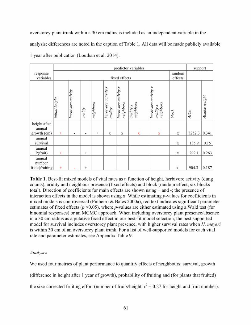
61

overstorey plant trunk within a 30 cm radius is included as an independent variable in the

analysis; differences are noted in the caption of Table 1. All data will be made publicly available

1 year after publication (Louthan et al. 2014).

response variables

predictor variables support

fixed effects random effects

initi

al h

eigh

t

herb

ivor

e ac

tivity

arid

ity

neig

hbor

s

herb

ivor

e ac

tivity

x

arid

ity

herb

ivor

e ac

tivity

x

neig

hbor

s

arid

ity x

ne

ighb

ors

herb

ivor

e ac

tivity

x

arid

ity x

ne

ighb

ors

bloc

k

AIC

c

Akai

ke w

eigh

t

height after annual

growth (cm) + - - + x x x x x 3252.3 0.341 annual

survival

x 135.9 0.15 annual P(fruit) + +

x 292.1 0.263

annual number

fruits|fruiting + - +

x 904.3 0.187 Table 1. Best-fit mixed models of vital rates as a function of height, herbivore activity (dung counts), aridity and neighbour presence (fixed effects) and block (random effect; six blocks total). Direction of coefficients for main effects are shown using + and -; the presence of interaction effects in the model is shown using x. While estimating p-values for coefficients in mixed models is controversial (Pinheiro & Bates 2000a), red text indicates significant parameter estimates of fixed effects (p ≤0.05), where p-values are either estimated using a Wald test (for binomial responses) or an MCMC approach. When including overstorey plant presence/absence in a 30 cm radius as a putative fixed effect in our best-fit model selection, the best supported model for survival includes overstorey plant presence, with higher survival rates when H. meyeri is within 30 cm of an overstorey plant trunk. For a list of well-supported models for each vital rate and parameter estimates, see Appendix Table 9.

Analyses

We used four metrics of plant performance to quantify effects of neighbours: survival, growth

(difference in height after 1 year of growth), probability of fruiting and (for plants that fruited)

the size-corrected fruiting effort (number of fruits/height: r2 = 0.27 for height and fruit number).

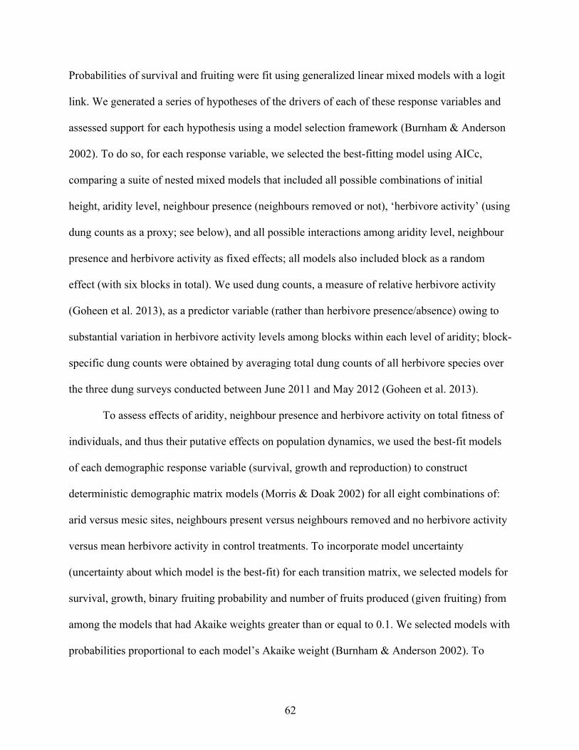
62

Probabilities of survival and fruiting were fit using generalized linear mixed models with a logit

link. We generated a series of hypotheses of the drivers of each of these response variables and

assessed support for each hypothesis using a model selection framework (Burnham & Anderson

2002). To do so, for each response variable, we selected the best-fitting model using AICc,

comparing a suite of nested mixed models that included all possible combinations of initial

height, aridity level, neighbour presence (neighbours removed or not), ‘herbivore activity’ (using

dung counts as a proxy; see below), and all possible interactions among aridity level, neighbour

presence and herbivore activity as fixed effects; all models also included block as a random

effect (with six blocks in total). We used dung counts, a measure of relative herbivore activity

(Goheen et al. 2013), as a predictor variable (rather than herbivore presence/absence) owing to

substantial variation in herbivore activity levels among blocks within each level of aridity; block-

specific dung counts were obtained by averaging total dung counts of all herbivore species over

the three dung surveys conducted between June 2011 and May 2012 (Goheen et al. 2013).

To assess effects of aridity, neighbour presence and herbivore activity on total fitness of

individuals, and thus their putative effects on population dynamics, we used the best-fit models

of each demographic response variable (survival, growth and reproduction) to construct

deterministic demographic matrix models (Morris & Doak 2002) for all eight combinations of:

arid versus mesic sites, neighbours present versus neighbours removed and no herbivore activity

versus mean herbivore activity in control treatments. To incorporate model uncertainty

(uncertainty about which model is the best-fit) for each transition matrix, we selected models for

survival, growth, binary fruiting probability and number of fruits produced (given fruiting) from

among the models that had Akaike weights greater than or equal to 0.1. We selected models with

probabilities proportional to each model’s Akaike weight (Burnham & Anderson 2002). To

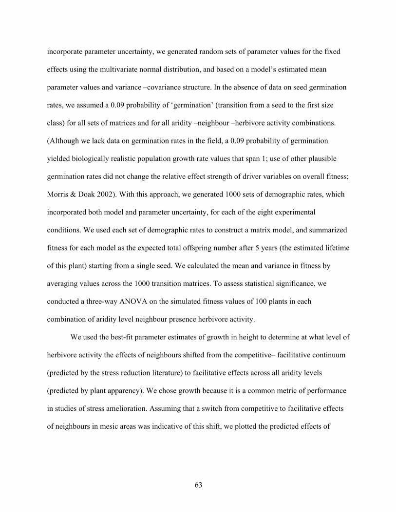
63

incorporate parameter uncertainty, we generated random sets of parameter values for the fixed

effects using the multivariate normal distribution, and based on a model’s estimated mean

parameter values and variance –covariance structure. In the absence of data on seed germination

rates, we assumed a 0.09 probability of ‘germination’ (transition from a seed to the first size

class) for all sets of matrices and for all aridity –neighbour –herbivore activity combinations.

(Although we lack data on germination rates in the field, a 0.09 probability of germination

yielded biologically realistic population growth rate values that span 1; use of other plausible

germination rates did not change the relative effect strength of driver variables on overall fitness;

Morris & Doak 2002). With this approach, we generated 1000 sets of demographic rates, which

incorporated both model and parameter uncertainty, for each of the eight experimental

conditions. We used each set of demographic rates to construct a matrix model, and summarized

fitness for each model as the expected total offspring number after 5 years (the estimated lifetime

of this plant) starting from a single seed. We calculated the mean and variance in fitness by

averaging values across the 1000 transition matrices. To assess statistical significance, we

conducted a three-way ANOVA on the simulated fitness values of 100 plants in each

combination of aridity level neighbour presence herbivore activity.

We used the best-fit parameter estimates of growth in height to determine at what level of

herbivore activity the effects of neighbours shifted from the competitive– facilitative continuum

(predicted by the stress reduction literature) to facilitative effects across all aridity levels

(predicted by plant apparency). We chose growth because it is a common metric of performance

in studies of stress amelioration. Assuming that a switch from competitive to facilitative effects

of neighbours in mesic areas was indicative of this shift, we plotted the predicted effects of

64

neighbours in the mesic and arid site as a function of herbivore activity and found the x-intercept

of the mesic line.

Results

For H. meyeri growth in the absence of large herbivores, our best-fitting model predictions were

generally consistent with the competition– facilitation continuum predicted by the stress-

reduction literature: neighbours slightly increased growth in arid areas and strongly decreased

growth in mesic areas (Figure 1a). In the presence of herbivores, however, neighbours increased

growth in both arid and mesic sites, with a weak facilitative effect in the arid site and a strong

facilitative effect in the mesic site (Figure 1b). In other words, the presence of herbivores

eliminated the interaction between neighbour presence and aridity on growth (indicated by

support for a three-way interaction among aridity, neighbours and herbivore activity; Table 1 and

Appendix, Table 9), suggesting that concealment by neighbours may be more important than

stress-mediation as a mechanism of facilitation in this large-herbivore-dominated system.

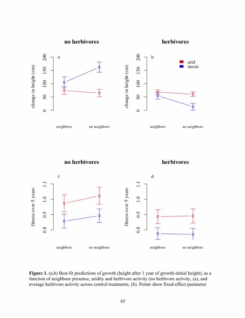
65

Figure 1. (a,b) Best-fit predictions of growth (height after 1 year of growth-initial height), as a function of neighbour presence, aridity and herbivore activity (no herbivore activity, (a), and average herbivore activity across control treatments, (b). Points show fixed-effect parameter

66

estimates and bars represent standard errors based on uncertainties of fixed-effect parameter estimates, without random effects. See Appendix Fig. 6 for a presentation of raw data using herbivore activity as a continuous predictor variable. (c,d) Projections of 5-year fitness of an individual seed as a function of neighbour presence, aridity and herbivore activity (zero herbivore activity, (c), and average herbivore activity across control treatments, (d)). Demographic projections incorporate model and fixed-effect parameter uncertainty for change in height, reproduction and survival, including all models with Akaike weights greater than or equal to 0.10. Error bars represent standard deviation across 1000 replicate deterministic projections. According to a three-way ANOVA with aridity, herbivore activity (zero herbivore activity versus average herbivore activity across control treatments) and neighbour presence (and all interactions among these main effects) as predictors, all main effects and the interaction between herbivore activity and neighbour presence are significant (p ≤ 0.05; Appendix Table 10). These models predict higher 5-year fitness in arid areas because probability of fruiting and number of fruits are higher in arid areas (presumably an evolutionary adaptation to counterbalance low germination probability and seedling survival; Louthan et al. 2013), but we assume similar seed set per fruit and germination rates in all matrices.

In contrast to neighbours’ effects on growth, neighbours did not exert strong effects on H.

meyeri reproduction; instead, negative effects of herbivory and positive effects of aridity were

important (Table 1). For survival, neither herbivory, neighbours nor aridity was important (Table

1).

Our results for the effects of neighbours on lifetime fitness were not consistent with the

predictions of the stress-reduction literature (Fig. 1c,d; Appendix Table 10). In the absence of

large herbivores, neighbours reduced projected fitness at both arid and mesic sites (Fig. 1c). By

contrast, there was no net effect of neighbours on fitness in unfenced control plots, suggesting

that facilitative effects in the presence of herbivores were strong enough to counterbalance the

competitive effects observed in herbivore exclosures (Fig. 1d; significant interaction between

neighbour presence and herbivore activity F = 4.3209, p = 0.038; Appendix Table 10). This

result supports the prediction from plant-apparency theory that neighbours should exert

facilitative effects in the presence of herbivores, but not in their absence.

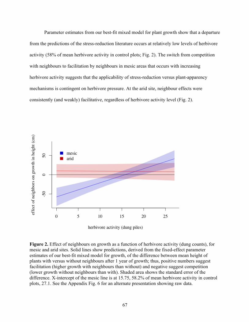
67

Parameter estimates from our best-fit mixed model for plant growth show that a departure

from the predictions of the stress-reduction literature occurs at relatively low levels of herbivore

activity (58% of mean herbivore activity in control plots; Fig. 2). The switch from competition

with neighbours to facilitation by neighbours in mesic areas that occurs with increasing

herbivore activity suggests that the applicability of stress-reduction versus plant-apparency

mechanisms is contingent on herbivore pressure. At the arid site, neighbour effects were

consistently (and weakly) facilitative, regardless of herbivore activity level (Fig. 2).

Figure 2. Effect of neighbours on growth as a function of herbivore activity (dung counts), for mesic and arid sites. Solid lines show predictions, derived from the fixed-effect parameter estimates of our best-fit mixed model for growth, of the difference between mean height of plants with versus without neighbours after 1 year of growth; thus, positive numbers suggest facilitation (higher growth with neighbours than without) and negative suggest competition (lower growth without neighbours than with). Shaded area shows the standard error of the difference. X-intercept of the mesic line is at 15.75, 58.2% of mean herbivore activity in control plots, 27.1. See the Appendix Fig. 6 for an alternate presentation showing raw data.

68

Discussion

In the absence of herbivory, our results for plant growth offer qualified support for the stress-

reduction literature, with neighbours weakly facilitating plant growth in arid areas and reducing

growth in mesic areas (Fig. 1a). In mesic areas, competitive effects of neighbours outweighed

any facilitative effects, such that the net effect of neighbours on plant growth was negative;

conversely, the net effect of neighbours was neutral-to-positive in arid areas, suggesting that

facilitative effects were at least as strong as competitive ones (Callaway 2007, Brooker &

Callaghan 1998, Armas et al. 2011). These competitive effects could include direct uptake of soil

water or rainfall interception, whereas facilitative effects could include amelioration of vapour

pressure deficit, increased soil water retention or reduced soil evaporation via shading

(Holmgren et al. 1997, Tielbörger & Kadmon 2000, Zou et al. 2005, Callaway 2007). Further

work would be necessary to establish which of these mechanisms are operating in our study

system.

Our results support the predictions of plant apparency in the presence of large herbivores.

In the presence of herbivores, neighbours enhanced growth regardless of abiotic stress level

(Fig.1b), and herbivores alleviated the competitive effects of neighbours on fitness (Fig. 1c,d).

Our work is consistent with the suggestion of Graff et al. (2011) that plant –plant interactions in

the presence of herbivores should primarily be facilitative. The effects of plant apparency were

strong enough to obscure the competition – facilitation continuum predicted by the stress-

reduction literature: in mesic areas, herbivores switched the net effect of neighbours from

competitive to neutral or facilitative (for fitness and growth, respectively). Thus, neighbours’

concealment of plants in mesic areas was strong enough to match or overwhelm neighbours’

stress-mediated competitive effects. In arid areas, facilitative effects were weak in the absence of

69

herbivores, and we did not find additional facilitative effects conferred by plant apparency in the

presence of herbivores, perhaps because of lower overall growth rates in arid areas.

Our results are consistent with theoretical predictions that the competition– facilitation

continuum predicted by stress reduction can be mitigated or even negated by herbivory (Smit et

al. 2009). In spite of these predictions, there have been few empirical tests of the relative strength

of stress amelioration versus plant apparency in ecosystems with extant herbivore communities

at densities comparable to historical records (Eskelinen 2007, Graff & Aguiar 2011, Solivered et

al. 2011). In a salt marsh community, Crain (2008) found that the effects of plant apparency were

weaker than those of stress reduction, an effect attributed to low and spatially variable herbivore

densities. In the absence of herbivores, Bulleri et al. (2011) found no support for the

competitive– facilitative continuum predicted by the stress-reduction literature; instead,

interactions between vermetid snails and macroalgae were always competitive. However, in the

presence of sea urchin herbivory, vermetids exerted a positive effect on macroalgae at

intermediate grazing pressure. These results show that the relative strength and sign of

neighbours’ effects can depend critically on herbivore density. Our results suggest that for intact

communities of large mammalian herbivores, the effects of plant apparency are stronger than the

competitive– facilitative effects of stress reduction. Our study further suggests that relatively low

herbivore densities can effect a switch from support for stress reduction to support for plant

apparency: our results show that a switch from net competition to net facilitation in mesic areas

occurs at around half of average herbivore activity levels (Fig. 2).

Effects of neighbours on lifetime fitness are complicated by vital rate- or life stage-

specific neighbour effects (Goldberg et al. 1999, Miriti 2006), and investigators rarely quantify

all of these stage-specific effects, limiting our understanding of the sum effect of neighbours on

70

plant fitness (Malkinson & Tielbörger 2010). Consistent with previous studies, our work shows

that neighbour effects vary for different vital rates. In contrast to strong effects on growth,

neighbours’ effects on reproduction and survival in H. meyeri were weak; instead, the direct

effects of aridity and herbivory were most important (Table 1 and Appendix Fig. 5).

Surprisingly, aridity has a positive effect on cumulative probability of reproduction and fruit

number, but these effects are likely mitigated by fewer reproductive events (Louthan et al. 2013).

Our integration of multiple vital rates into a summed fitness metric shows that, in this system, the

overall effect of neighbours on fitness is inconsistent with the predictions of the stress-reduction

literature, likely because the effect of growth rate is diluted by effects of aridity and herbivores

on reproduction and survival (Fig. 1c). Our results are consistent with those of the only other

experimental study of which we are aware that has synthesized neighbours’ effect on lifetime

fitness in different stress environments (Stanton-Geddes et al. 2012). Because quantifying the

total effect of neighbours on fitness is critical to assessing whether neighbours and aridity exert

biologically relevant effects on population dynamics, additional studies along these lines would

be valuable.

We assumed identical seed germination rates across all of our demographic projections,

largely because we lack the requisite data to quantify germination rates under field conditions;

however, our results on 5-year (approx. lifetime) fitness are robust to this (probably incorrect)

assumption. First, seed germination rates are probably higher in mesic areas, increasing overall

fitness in mesic areas to levels approaching those found in arid areas (Fig. 1c,d), but not

changing the direction of the effect of neighbours. Second, neighbours probably increase 5-year

fitness by increasing seedling germination rates (e.g. by providing safe sites or reducing seedling

desiccation; Callaway 2007). It is possible that neighbours’ facilitation of 5-year fitness via

71

seedling facilitation is strong enough to counteract their observed competitive effects in the

absence of herbivory (Fig. 1c). However, in the presence of herbivores, this effect will only serve

to increase the facilitative effects of neighbours; thus, incorporating neighbours’ facilitation of 5-

year fitness would likely still show results consistent with plant apparency.

Most empirical tests of the stress-reduction literature have been conducted in places

where large mammalian herbivores are either not present or have been functionally extirpated; as

a result, we have a poor understanding of how large consumers might affect the competition–

facilitation continuum arising from abiotic stress reduction. Determining how plant–plant

interactions shape plant performance is a critical first step in assessing how these interactions

shape community structure, but our results highlight that such interactions hinge critically on the

top-down effects of herbivores. Considering the effects of plant–plant interactions in the context

of higher trophic levels—particularly in ecosystems that harbour diverse, intact assemblages of

large mammals—will provide a more complete picture of community dynamics.

Acknowledgements

We thank A. Eshwa, K. Elkana, R. Shriver, J. Lomuria, S. Lima and A. Hussein for field

assistance, Mpala Research Centre for logistical support, and the Government of Kenya for

permission to conduct research.

Data accessibility

Dataset will be uploaded onto the Dryad data repository 1 year following publication.

Funding statement

A.M.L. received funds from NSF DEB-0812824, a L’oréal-UNESCO fellowship and from the

University of Wyoming (President’s Fund, Berry Center Avian Ecology Fund, Cheney

International Fellowship for Excellence, Haub Creative Activities Grant, Menkens Memorial

72

Scholarship, Women in Conservation Biology scholarship, Plummer Grant, and Menkens

Memorial Scholarship). The UHURU experiment has been funded via a NSERC Discovery

grant, NSERC Research Tools and Instruments grant, funds from the University of British

Columbia and the University of Wyoming to J.R.G., funds from the University of Florida to

T.M.P., and NSF OISE-0852961 to R.M.P.

73

CHAPTER 5

SPECIES INTERACTIONS MORE STRONGLY AFFECT POPULATION GROWTH RATE IN UNSTRESSFUL AREAS

Abstract

Understanding the forces that determine the origin and maintenance of species range limits is one

of the central questions of ecology (Gaston 2003) with implications for both biodiversity of

natural communities and climate change impacts on species distribution patterns (Parmesan

2006). Two broad classes of factors constrain species ranges: abiotic factors, such as temperature

and precipitation, and species interactions such as predation and herbivory (Sexton et al. 2009).

However, we lack a clear understanding of when and where each of these classes of factors

operates most strongly. A hypothesis dating back to Darwin suggests that abiotic factors more

often set limits in stressful areas, while species interactions dominate in more benign

environments (Louthan et al. 2015). Despite the widespread assumption that this is a powerful

generality, we have little empirical evidence that directly tests the idea. Here, we report strong

support for this pattern from a series of experimental manipulations conducted across a sharp

aridity gradient. We find stronger effects of herbivory, neighboring plants, and pollination

limitation on estimated population growth rate of our focal plant species in mesic areas. We also

show that larger effects of interactions in less stressful areas arise because of changes in the

responsiveness of population growth to these effects with stress (Louthan et al. 2015), rather than

higher densities or diversities of interactors in less stressful areas, commonly assumed to be the

primary generating mechanism starting with Darwin (1859). Our results suggest that this pattern

may occur across a wide variety of taxa with similar life histories and effects of species

74

interactions on vital rates. This work supports theoretical predictions concerning the factors

setting range limits, provides new understanding about why these shifting effects occur, and has

implications for understanding when and where we need to consider species interactions in both

biodiversity studies and projections of species’ ranges shifts.

Introduction

What sets and maintains species range limits is one of the fundamental questions of ecology and

evolution (Gaston 2003), and also has profound implications for projections of the ecological

effects of climate change (Parmesan 2006). While we know that abiotic conditions often set

species range limits (Sexton et al. 2009), both long-standing theory (Darwin 1859) and a few

empirical studies (reviewed in Sexton et al. 2009) show that species interactions, such as

predation, competition, or parasitism, can also be important factors limiting population growth at

species range limits. However, we lack a well-supported framework for predicting when and

where each of these classes of factors might be most important. One long-standing but little-

tested hypothesis predicts that abiotic stress should most often set range limits in apparently

stressful environments, while species interactions should exert stronger effects in apparently

benign environments (we refer to this idea, first proposed by Darwin (1859), as the Species

Interactions-Abiotic Stress Hypothesis, SIASH; Louthan et al. 2015). Some small-scale studies

have clearly supported this predicted pattern of effects (especially in intertidal systems; Connell

1961a,b), and correlational data suggest that it might exist across elevations (Ettinger et al. 2011)

and latitudes (Sanford et al. 2003). Indeed, it has been cited as the main reason for lack of

consistent, predicted shifts in the trailing edge of species range limits in recent climate change

studies (Ettinger et al. 2011, Sunday et al. 2012). However, other studies have found

contradictory evidence (Louthan et al. 2015) and to date we have few clear tests of the idea,

75

particularly experimental tests, and none that quantify the importance of multiple species

interactions on population performance or test for why such effects might arise.

The foundational assumption of SIASH asserts that species interactions exert stronger

effects on population growth rate in unstressful areas, ultimately setting distributional limits by

driving populations into decline. We tested this hypothesis for multiple species interactions

across a rainfall gradient, using Hibiscus meyeri, a model plant species in East Africa that occurs

across a substantial range of aridities (Louthan et al. 2013, Louthan et al. 2014). Hibiscus meyeri

is a common subshrub in this acacia-dominated semi-arid savanna that experiences rainfall

limitation (see Appendix), both competitive and facilitative effects from grasses and shrubs

(Louthan et al. 2014), is browsed by a wide array of herbivores (Louthan et al. 2013), and

appears to undergo delayed autonomous self-pollination that favors outcrossing while still

ensuring self-pollination if outcross pollination does not occur (see Appendix; Ruiz-Guajardo

2008). Across three sites that span a substantial aridity gradient (22% higher rainfall in our Mesic

than Arid Site), we collected demographic data on unmanipulated plants and plants within a

nested set of experimental treatments including herbivore exclosures and neighbor removals

(Goheen et al. 2013; Appendix). We used data collected over 4 years to estimate effects of

multiple factors on survival, growth, and reproduction, and used these vital rate functions to

construct demographic models that estimate population growth rate, λ, as a function of aridity

(including both temporal and spatial variation), plant neighbors (we focus here on grass and

herbaceous neighbors, which we experimentally manipulated, rather than trees and shrubs),

mammalian herbivores, and pollinators (which were not manipulated in the field; see Appendix);

this unified demographic approach allows us to both predict differences in population growth

rate and dissect the mechanisms driving these changes.

76

Results and Discussion

In this system, SIASH predicts that species interactions exert stronger effects on

population growth rate in mesic than in more arid areas. Consistent with this prediction, we find

that all three species interactions (herbaceous neighbors, herbivores, and pollinators) exert

stronger effects on λ in the Mesic Site (Fig. 1; woody plants were not considered here). The

interacting effects of neighbors and herbivores are subadditive, such that neighbors exert some

facilitative effects in the presence of herbivores (reducing the magnitude of their competitive

effect), likely due to plant apparency effects (Fig. 1D; Louthan et al. 2014). However, the net

effect of neighbors and herbivores together was still stronger in our Mesic Site. Similarly,

pollinators increase λ substantially more in the Mesic Site; in combination with neighbors and

herbivores these effects are also subadditive, such that adding pollinators to populations that

have herbivores and neighbors has a weaker positive effect than adding pollinators to

populations with no interactions. This subadditivity likely arises from negative effects of

herbivores on reproduction (Fig. 2) and of neighbors on fruit-to-seedling transition (Appendix

Table 11).

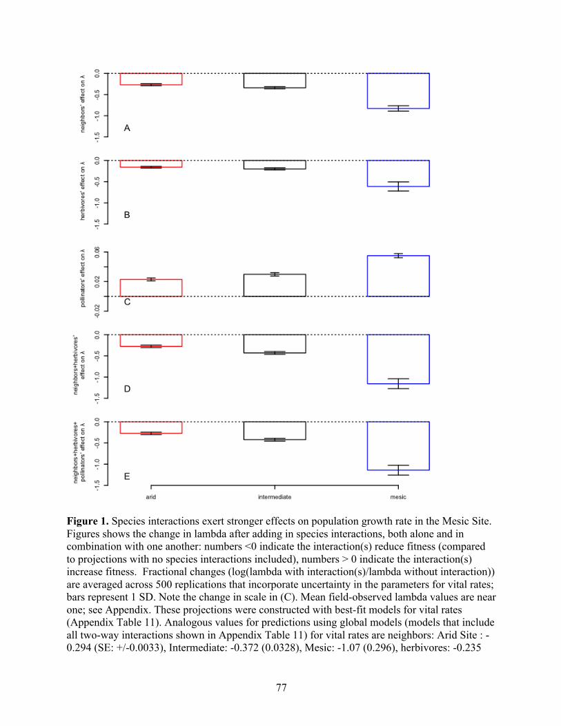
77

Figure 1. Species interactions exert stronger effects on population growth rate in the Mesic Site. Figures shows the change in lambda after adding in species interactions, both alone and in combination with one another: numbers <0 indicate the interaction(s) reduce fitness (compared to projections with no species interactions included), numbers > 0 indicate the interaction(s) increase fitness. Fractional changes (log(lambda with interaction(s)/lambda without interaction)) are averaged across 500 replications that incorporate uncertainty in the parameters for vital rates; bars represent 1 SD. Note the change in scale in (C). Mean field-observed lambda values are near one; see Appendix. These projections were constructed with best-fit models for vital rates (Appendix Table 11). Analogous values for predictions using global models (models that include all two-way interactions shown in Appendix Table 11) for vital rates are neighbors: Arid Site : -0.294 (SE: +/-0.0033), Intermediate: -0.372 (0.0328), Mesic: -1.07 (0.296), herbivores: -0.235

78

(0.0384), -0.276 (0.0423), -0.846 (0.3416), pollinators: 0.023 (0.0022), 0.031 (0.0025), 0.06 (0.0052), neighbors + herbivores: -0.305 (0.0382), -0.475 (0.0407), -1.378 (0.3366), neighbors+ herbivores+ pollinators: -0.302 (0.038), -0.424 (0.0298), -1.155 (0.1286). For comparison, see Appendix Fig. 7 for an analogous figure that includes only per-capita effects of species interactions (projections without block effects and with the same interactor densities at all rainfall levels).

Figure 2. Effects of rain and species interactions on vital rates are reasonable. Figure shows the direction of fixed effect coefficients (initial biomass, rainfall, neighbor density, herbivore activity, and distance to woody plant; woody plants here are acacia and Euphorbia nyikae; see Appendix) for best-fit models of each vital rate (interactions, if present in the best-fit model, are shown in right-most bar; see Appendix Table 11). See Appendix Table 11 for fixed-effect estimates for variance in growth. Absence of bars indicates that fixed effect was not present in the best-supported model. Bars indicate standard error of coefficients. All coefficients are from models fit with standardized predictor variables, so magnitude of values reflects relative effect

79

size. Effects on variance in growth and fruit to seedling transition are shown in Appendix Table 11.

Several different mechanisms could explain the pattern of greater species interaction

effects in more mesic areas. First, there may be higher density and diversity of interactors (e.g.,

herbivores, plant neighbors) in mesic areas: many of the earliest and most well-known advocates

of the SIASH pattern suggest that this is the main driver of stronger effects on population growth

rate in more benign environments (Darwin 1859; MacArthur 1972; we refer to these as “density

effects”). Second, each interactor might exert stronger effects on individual vital rates in benign

areas (“per capita demographic impact”; note that our vital rate functions show per interactor or

interaction effects); for example, an herbivore could consume more H. meyeri in mesic areas,

perhaps due to higher plant palatability, or due to patchier populations with higher local

population densities, making plants easier to find. Finally, stress might change the life history of

a species such that the same effects of interactors on vital rates would have stronger population-

level effects in mesic areas (“life history effects”). For example, if sensitivity of populations in

mesic areas to size-specific survival is higher than in arid areas, then herbivores’ reduction of

survival will have more substantial effects on λ in the Mesic Site. We decomposed these

different effects by estimating changes in lambda that would result from these separate aspects of

species interactions, quantifying the relative contribution of each effect (see Appendix). This

decomposition shows that for all interactions, by far the most important driver of stronger effects

of species interactions in the Mesic Site is life history effects (Fig. 3A-C). Only for neighbors is

there any effect of density in generating this pattern, and in the case of herbivory, density effects

actually result in stronger effects in Arid Sites (our system has higher herbivore densities in arid

areas, the opposite of most systems; McNaughton et al. 1989, Salazar & Marquis 2012). This

80

result is in direct contrast to the oft-cited density effects that researchers assume drive most of

the SIASH pattern (Louthan et al. 2015).

Figure 3. The life history mechanism drives support for the SIASH, with the majority of the effect generated by fruit-to-seedling transition rates. Figure shows the decomposition of the factors creating greater effects of species interactions on population growth rates (λ) in the Mesic v. Arid Site. The response variable in all panels, ∆∆𝜆, is the difference between estimated lambda without and with each species interaction in the Mesic Site, minus the same difference for the Arid Site, and then rescaled to equal 1 for the observed full effect on lambda. A-C) The contribution of density effects, per-capita demographic effects, and life history effects to the total SIASH pattern seen in neighbor, herbivore, and pollination interactions. D-F) The contributions of individual vital rates (where reproduction includes both probability of reproduction and the number of fruits produced| reproduction) to generation of the SIASH pattern. “Total” bars serve as a reference for the total net effect of an interaction. Negative numbers indicate effects that contradict the main effect; for example, life history effects in neighbors weaken the net negative effects of neighbors in the Mesic Site. Numbers >1 indicate that some of that effect’s interaction

81

is negated by contrasting effect of other mechanisms. See Appendix Table 14 for the contribution of variance in growth, and Appendix Fig. 8 for sensitivities of lambda to individual vital rates.

A second, orthogonal approach to decomposing effects on population growth is to dissect

how the effect of a species interaction on each vital rate influences overall differences in

interaction strengths in Arid vs. Mesic Sites. Individually, the effects of each factor on different

vital rates were consistent with our expectations: rainfall increased several aspects of H. meyeri

performance (growth, and two components of reproduction; Fig. 2); herbivores had negative

effects on these three vital rates (Fig. 2); neighbors decreased growth rates (Fig. 2) and fruit-to-

seedling transition rates (Appendix Table 11); and distance to woody plants increased

reproduction (Fig. 2). Despite these diverse effects, for all species interactions, effects on the

fruit to seedling transition generate the majority of stronger effects of species interactions in the

Mesic Site (Fig. 3D-F), likely due to H. meyeri population growth being sensitive to this vital

rate (Appendix Fig. 8). These results suggest that the population-level effect of species

interactions can in some cases be distilled to effects on one vital rate (making future studies of

species interactions simpler, if researchers can identify that key vital rate).

It is not clear how commonly life history will generate stronger effects of species

interactions in unstressful places, simply because we have limited data on how sensitivities of

populations vary with stress, and sensitivity patterns can vary with life history strategy. Further,

if species interactions do not happen to affect the vital rates to which populations are sensitive,

we would likely see little support for SIASH. For example, in the case of herbivory, predation or

parasitism, these interactions might exert no or weak effects on vital rates in unstressful areas,

because unstressed victims are able to compensate for damage (as we may be seeing here in the

case of herbivory; Maschinski & Whitman 1989), are less susceptible to attack, or more able to

82

combat infection (Nelson & Demas 1996, Wirsing et al. 2002). Although it is difficult to

generalize about the importance of the life history mechanisms generating the SIASH across

species (particularly since this effect arises largely due to sensitivity to just one vital rate), our

consistent results on multiple species interactions suggest that life history effects may be

universally important.

Our findings add experimental support for a foundational assumption of a long-held but

poorly-tested hypothesis concerning the forces governing range limits, and suggest that clear and

consistent patterns in the control of population growth rate and hence range limits may exist.

Concomitant with the lack of abiotic control over some warm-edge limits (Ettinger et al. 2011,

Sunday et al. 2012), our results suggest that species interactions could be driving many trailing-

edge or tropical range limits, even without gradients in interactor density (Darwin 1859,

MacArthur 1972) or interaction frequency (Schemske et al. 2009). In particular, our results

caution against ignoring or minimizing effects of species interactions in setting range limits

(Afkhami et al. 2014, Tingley et al. 2014) or in predicting future distribution patterns (Van der

Putten et al. 2010, Blois et al. 2013, Raffa et al. 2013, Wisz et al. 2013), but we also provide a

heuristic framework for when and where species interactions might be most important within a

species range, and where they might be less important.

Materials and Methods

We worked at the Mpala Research Centre in central Kenya, in a semi-arid acacia-

dominated savanna just off the equator, with little variation in temperature and a relatively intact,

diverse herbivore community (see Appendix). We used a large-scale herbivore-exclusion

experiment arrayed across a pronounced rainfall gradient (UHURU; Ungulate Herbivory Under

Rainfall Uncertainty; Goheen et al. 2013); UHURU is comprised of an open control with three

83

highly effective exclosures (see Appendix) that exclude different sized- guilds of herbivores,

replicated three times (“blocks”) at each of three sites across this rainfall gradient. Total rainfall

increases 22% from the Arid to Mesic Site (Appendix Table 12), and soil characteristics do not

vary substantially across this gradient (Goheen et al. 2013). We used rain gauges to get rainfall

values, and we used quarterly herbivore dung counts (see Goheen et al. 2003) as a proxy for

herbivore activity (see Appendix). Herbivore community composition is similar across sites,

with elephant (Loxodonta africana), impala (Aepyceros melampus) and dik-dik (Madoqua

guentheri) dominating (Louthan et al. 2014). In this ecosystem, Hibiscus meyeri is a common,

apparently moderately palatable subshrub with no known chemical or physical defenses, which

exhibits moderate compensatory regrowth following herbivory events. It is heavily browsed by

many different herbivore species and experiences water limitation (Appendix). Flowers in H.

meyeri present their style for insect-mediated outcross pollination, but also have a mechanism to

touch their style to their anthers (presumably self-pollinating themselves) if no insects visit (A.

Louthan, pers. obs). Self pollination is very common, but bouts of outcrossing can also occur

(see Appendix), suggesting inbreeding depression is likely.

To quantify the importance of rainfall and herbivory on plant vital rates, between June

24- August 5 2011 we exhaustively searched randomly selected areas in all Sites and exclosure

treatments (controlling for plant phenology; Louthan et al. 2013), as well as in transects outside

of the UHURU experiment (coded as a separate block in our analyses) and marked and mapped

all H. meyeri individuals, measuring size, reproduction, and neighbor cover in a 30 cm radius

(see sample sizes in Appendix Table 13). Until 2014, we returned annually to remeasure these

plants, also noting survival and distance to nearest woody plant (acacia, Vachellia sp and

Senegalia sp, as well as Euphorbia nyikae, Croton sp, Grewia sp, Balanities sp, or Boscia sp) >

84

30 cm tall. We marked new plants in the same area to replace those that died, measuring 1719

unique individuals throughout the experiment.

To quantify the effect of neighbors on plant vital rates, we marked and measured

haphazardly chosen plants in the full exclosures and open controls at all levels (see Louthan et al.

2014), as well as on transects outside of the UHURU experiment, randomly assigned 1/3 of them

to a neighbor removal treatment, and cut down all biomass within a 30 cm radius, carefully

painting the cut stalks with Roundup®. We removed this biomass every 6 months, and

remeasured both unmanipulated and neighbor-removed plants annually, replacing dead or

missing plants as necessary, resulting in 1504 individuals total (Appendix Table 13).

We used work on a congeneric species with a similar floral phenotype (Hibiscus trionum;

Seed, Vaughton, and Ramsey 2006; see Appendix) to simulate a release from inbreeding

depression caused by increased pollinator visitation rates. Our pollinator treatments, which

assume that all fruits we observed in the field were selfed, represents a shift from no outcross

pollination to all outcross pollination (both likely outcomes; field observed per-plant pollination

rates are usually either none or all of flowers; see Appendix). Thus, our results represent the

maximum possible effect pollinators could exert in this system.

Finally, we obtained fruit to seedling transition rates by counting all seedlings in a 2m

radius around 118 highly fecund individuals arrayed across rainfall levels and herbivore

exclosure combinations, once just after the dry season and once after the wet season. Seedlings

entered the population with a height of 5.44 cm & a basal area of 0.96, the mean of all H. meyeri

with height< 10 & a basal diameter of 2 (the upper limits for seedlings in the field; A. Louthan

pers. obs).

85

We used a model selection framework to select best-fit mixed models for survival,

growth, variance in growth, probability of reproduction, and number of fruits produced given

reproduction. We found the best model from all subsets of a global model with initial biomass

and all two-way interactions between rain (measured as site-and year-specific rainfall totals),

herbivore activity, neighbor cover, and distance to nearest woody plant as fixed effects. Block

and plant-measurer (of initial plant size) were random effects (see Appendix). We provide

estimates of change in λ using global models in the figure legends. We first ensured that each

subset of our data (unmanipulated plants, unmanipulated haphazardly selected plants, and

unmanipulated plants within and outside of the UHURU experiment; Appendix) did not unduly

change the parameter estimates of the global model. To obtain fruit to seedling transition rates,

we divided seedling number by fruit number, and used a similar mixed model selection approach

to select the best model for log-transformed seedlings per fruit, comparing all subsets of a global

model with all interactions among rain, herbivore activity, and neighbor cover as fixed effects,

and with block as a random effect (all the measurements were done by the same measurer).

Hibiscus meyeri fruits have a maximum of 15 seeds (A. Louthan, pers. obs.), so we fixed the

maximum seedlings per fruit at 15.

We used the model with the highest AIC weight for each vital rate to construct

deterministic demographic matrices for 6 combinations of species interactions (none, +

neighbors, + herbivory, + pollination, + herbivory & neighbors, + herbivory & neighbors &

pollination) at each aridity level. We incorporated parameter uncertainty by sampling from the

multivariate distribution of fixed effect parameter estimates (Appendix Table 11) and calculating

each of the 6 above matrices for each set of parameter values. We show projections that include

block effects and rainfall level x herbivore exclosure –specific predictor values (herbivore

86

activity, neighbor cover, and distance to woody plant) in the main text. We show projections

without block effects and with non- specific predictor values in the supplemental information;

these include no effects of density nor unmeasured differences across levels (Appendix Fig. 7;

effects in the Mesic Site are greater than effects in the Arid Site).

To understand whether per-capita demographic rates, sensitivities, or densities effect

larger changes in λ in mesic areas, we decomposed the change in λ in Mesic v. Arid Sites into

each of these three components. For each species interaction, we calculated  ∆𝜆  

(𝜆!"#$#%&#  !"  !"#$%#!  !"#$%&'#!("-𝜆!"#$%&$  !"  !"#$%#!  !"#$%&'#!(") for both Mesic (∆𝜆!) and Arid

(∆𝜆!) Sites to obtain ∆∆𝜆   =  ∆𝜆! − ∆𝜆!. For each interaction, we then estimated both the total

value for ∆∆𝜆 and the value for ∆∆𝜆 when two types of effects were removed from the

calculation (Appendix Table 14). We calculated three ∆∆𝜆’s that set different effects to mean

values:

1. focal species interactor densities

2. rain terms in rain* focal species interaction terms

3. block effects and rainfall in all other terms

Letting (1) vary represents varying interactor density with rainfall, (2) represents the variation in

per-capita demographic rates, and (3) represents the variation in life history effects. For this

calculation, we used the mean of the Mesic and Arid Site values of other predictor variables

(besides rainfall and the focal species interaction; e.g., for the contribution of neighbors, we set

herbivore and distance to woody plant to their mean value in Mesic and Arid Sites’ full herbivore

exclosure treatments, and pollinators to zero) to isolate the effect of rainfall and the species

interaction of interest.

87

Finally, to assess which vital rates contributed most to ∆∆𝜆, we used a similar approach,

setting block effects and the rainfall terms for individual vital rates to the mean value to obtain

the fractional contribution of each vital rate to the sum  ∆∆𝜆.  

88

CHAPTER 6

CONCLUSION

In the study system that was my focus in this work, species interactions exert stronger effects on

population growth rate in less stressful areas. Neighbors and herbivores exert stronger negative

effects in mesic areas, and pollinators exert stronger positive effects in these same more mesic

habitats. However, predicting population growth rates of Hibiscus meyeri subjected to multiple

species interactions is not as straightforward: for example, herbivores modify the effect of

neighbors, such that neighbors exert some positive effects in the presence of herbivores due to

plant apparency. Further, these effects appear to be most often mediated by changes in the

sensitivity to population growth rate to different vital rates with changing rainfall, such that small

differences in the effect of species interactions on vital rates are amplified by large sensitivities

to those vital rates in mesic areas, resulting in a strong net effect on population vital rate. These

results have important implications for our understanding of species range limits, as well as for

our predictions of shifts in species range limits.

Several added complexities were also revealed in my work regarding patterns in the

strength of species interactions across stress gradients. For example, my third chapter shows that

while herbivores exert stronger levels on population-level performance (e.g., abundance) in

mesic areas, they exert weaker effects on individual performance (e.g., the reduction herbviores

have on individual plants’ growth rate). My fifth chapter shows similar effects; though we see

stronger effects of herbivores on population growth rate in mesic areas, for at least some vital

rates (e.g., growth) we see stronger effects of herbivores in arid, not mesic, areas. This

discrepancy arises due to changes in the sensitivity of population growth rate to growth in mesic

89

v. arid areas. These findings suggest that studies of individual-level plant response to herbivores

do not necessarily translate up to responses of plants at the population or abundance level. Thus,

studies that look at changes in plant abundance or community composition should address

multiple levels of plant performance.

Herbivores and neighbors also interact in complex ways that modify the importance of

species interactions across stress gradients. Neighbors exert competitive effects on H. meyeri, but

also appear to confer protection from herbivores due to plant apparency effects. Thus, the effect

of neighbors on H. meyeri is different in the presence v. absence of herbivores, and relatively

low herbivore densities (only half of what we see in the field) alter the net effect of neighbors on

H. meyeri performance. Interestingly, predictions of the recent ecological literature (that

neighbors exert facilitate effects in arid areas, but competitive effects in mesic areas) enjoy little

support in our system, particularly for components of fitness.

In spite of these complications, using all the data I collected during my dissertation to

parameterize demographic models that include multiple effects on population growth, I find that

herbivores, neighbors, and pollinators (all of the species interactions I studied in my dissertation)

have stronger effects in mesic areas. These results provide strong support for the predictions of

the species interactions-abiotic stress hypothesis (SIASH; see Chapter 2): neighbors, herbivores

and pollinators exert stronger effects on populations in mesic areas than in arid areas. Neighbors

exert the strongest effect (competitive, but with some facilitative effects in the presence of

herbivores), herbivores an intermediate, negative effect, and pollinators the weakest, positive

effect. Higher densities of interactors in mesic areas are not the primary driver of this pattern.

Instead, changes in the sensitivity of population growth rate to vital rates result in stronger

effects of species interactions in mesic areas.

90

This work provides support for a broad, long-standing, but relatively untested, hypothesis

concerning the origin of and persistence of species range limits. There is still a dearth of

empirical evidence testing this idea, despite the fact that it is often assumed to be a strong

generality. In particular, there are four non-independent mechanisms that may govern the

strength of species interactions and could result in the SIASH-predicted pattern, both at the level

of plant response and at the community level. However, these mechanisms do not necessarily

lead to SIASH-like patterns in nature. In trying to address these questions, my work is

particularly novel in its synthetic approach that includes data on multiple types of species

interactions, its focus on aridity as a stressor, and the relatively well-preserved ecosystem that

still has many species interactions intact. Further work on this system will try to dissect the role

of different size-guilds of herbivores as a function of abiotic stress, using the UHURU

experimental setup, as well as expand on the implications for species distribution models by

recommending locations where these models should include species interactions.

91

BIBLIOGRAPHY

Afkhami, ME, McIntrye, PJ, and Strauss, SY. 2014. Mutualist-mediated effects on species’

range limits across large geographic scales. Ecology Letters 17, 1265–1273

Alberti, J, Escapa, M, Iribarne O, Silliman, B, and Bertness, M. 2008. Crab herbivory regulates

plant facilitative and competitive processes in Argentinean marshes. Ecology 89, 155 –

164

Anderson, RP, Peterson, AT, and Gómez-Laverde, M. 2002. Using niche-based GIS modeling to

test geographic predictions of competitive exclusion and competitive release in South

American pocket mice. Oikos 98, 3–16

Anderson, TM and Frank, DA. 2003. Defoliation effects on reproductive biomass: importance of

scale and timing. Journal of Range Management 56, 501–516

Anderson, TM, Ritchie, ME, and McNaughton, SJ. 2007. Rainfall and soils modify plant

community response to grazing in Serengeti National Park. Ecology 88, 1191–1201

Angert, AL. 2009. The niche, limits to species’ distributions, and spatiotemporal variation in

demography across the elevation ranges of two monkey flowers. Proceedings of the

National Academy of Sciences U.S.A. 106, 19693

Angert, AL, LaDeau, SL, and Ostfeld, RS. 2013. Climate change and species interactions: ways

forward. Annals of the New York Academy of Sciences 1297, 1–7

Aragón, P and Sánchez-Fernández, D. 2013. Can we disentangle predator–prey interactions from

species distributions at a macro-scale? A case study with a raptor species. Oikos 122, 64–

72

Armas, C, Rodríguez-Echeverría S, and Pugnaire, FI. 2011 A field test of the stress–gradient

hypothesis along an aridity gradient. Journal of Vegetation Science 22, 818– 27

92

Armbruster, P, and Reed, D. 2005. Inbreeding depression in benign and stressful environments.

Heredity 95, 235-242

Augustine, DJ. 2010 Response of native ungulates to drought in semi-arid Kenyan rangeland.

African Journal of Ecology 48, 1009 – 1020

Bakker ES, Dobrescu I, Straile D, and Holmgren M. 2013. Testing the stress gradient hypothesis

in herbivore communities: facilitation peaks at intermediate nutrient levels. Ecology 94,

1776– 1784

Bakker, ES, Ritchie, ME, Olff, H, Milchunas, DG and Knops, JMH. 2006. Herbivore impact on

grassland plant diversity depends on habitat productivity and herbivore size. Ecology

Letters 9, 780–788

Beddington, JR, Free, CA, and Lawton, JH. 1978. Characteristics of successful natural enemies

in models of biological-control of insect pests. Nature 273, 513–519

Bertness MD and Callaway R. 1994. Positive interactions in communities. Trends in Ecology

and Evolution 9, 191 – 193

Bingham, RA and Ort, AR. 1998. Efficient pollination of alpine plants. Nature 391 238-239

Birch, LC. 1953. Experimental background to the study of the distribution and abundance of

insects: I. The influence of temperature, moisture and food on the innate capacity for

increase of three grain beetles. Ecology 34, 698–711

Blois, JL, Zarnetske, PL, Fitzpatrick, MC, and Finnegan, S. 2013. Climate change and the past,

present, and future of biotic interactions. Science 341, 499–504

Boyce, MS, Haridas, CV, Lee, CT, Boggs, CL, Bruna, EM, Couson, T, Doak, D, Drake, JM,

Gaillard, JM, Horvitz, CC, Kalisz, S, Kendall, BE, Knight, T, Mastrandrea, M, Menges,

93

ES, Morris, WF, Pfister, CA, and Tuljapurkar, SD. 2006. Demography in an increasingly

variable world. Trends in Ecology and Evolution 21, 141–148

Brooker RW and Callaghan TV. 1998 The balance between positive and negative plant

interactions and its relationship to environmental gradients: a model. Oikos 81, 196– 207

Brown, JH. 1971. Mechanisms of competitive exclusion between two species of chipmunks.

Ecology 52, 305-311

Brown, JH. 1995. Macroecology, University of Chicago Press

Bulleri, F, Cristaudo, C, Alestra, T, and Benedetti-Cecchi, L. 2011 Crossing gradients of

consumer pressure and physical stress on shallow rocky reefs: a test of the stress-gradient

hypothesis. Journal of Ecology 99, 335– 344

Bullock, JM, Edwards, RJ, Carey, PD, and Rose, RJ. 2000. Geographical separation of two Ulex

species at three spatial scales: does competition limit species’ ranges? Ecography 23,

257–271

Burnham KP, Anderson DR. 2002. Model selection and multimodel inference, Springer

Cahill, AE, Aiello-Lammens, ME, Fisher-Reid, MC, Hua X, Karanewsky, CJ, Ryu, HY, Sbeglia,

GC, Spagnolo, F, Waldron, JB, Warsi, O, and Wiens, JJ. 2013. How does climate change

cause extinction? Proceedings of the Royal Society of London B: Biological Sciences

280, 20121890

Callaway, RM. 2007 Positive interactions and interdependence in plant communities, Springer.

Callaway, RM, Brooker, RW, Choler, P, Kikvidze, Z, Lortie, CJ, Michalet, R, Paolini, L,

Pugnaire, FI, Newingham, B, Aschehoug, ET, Armas, C, Kikodze, D, and Cook, BJ.

2002. Positive interactions among alpine plants increase with stress. Nature 417, 844-848

94

Case, TJ, Holt, RD, McPeek, MA, and Keitt, TH. 2005. The community context of species’

borders: ecological and evolutionary perspectives. Oikos 108, 28–46

Caswell, H. 2001. Matrix Population Models, Sinauer Associates, Inc.

Chase, JM, Leibold, MA, Dowling, AL and Shurin, JB. 2000. The Effects of Productivity,

Herbivory, and Plant Species Turnover in Grassland Food Webs. Ecology 81, 2485–2497

Coley, PD and Aide, TM. 1991. Comparison of herbivory and plant defenses in temperate and

tropical broad-leaved forests. In Plant–Animal Interactions: Evolutionary Ecology in

Tropical and Temperate Regions (Price, P.W. et al., eds), pp. 25–49, Wiley

Connell, JH. 1961a. Effects of competition, predation by Thais lapillus, and other factors on

natural populations of the barnacle Balanus balanoides. Ecological Monographs 31, 61–

104

Connell, JH. 1961b. Influence of interspecific competition and other factors on distribution of

barnacle Chthamalus stellatus. Ecology 42, 710-723

Covey, C, AchutaRao, KM, Cubasch, U, Jones, P, Lambert, SJ, Mann, ME, Phillips, TJ, and

Taylor, KE. 2003. An overview of results from the Coupled Model Intercomparison

Project. Global and Planetary Change 37, 103-133

Crain, CM. 2008. Interactions between marsh plant species vary in direction and strength

depending on environmental and consumer context. Journal of Ecology 96, 166 – 173

Crimmins, SM, Dobrowski, SZ, Greenberg, JA, Abatzoglou, JT, and Mynsberge, AR. 2011.

Changes in climatic water balance drive downhill shifts in plant species’ optimum

elevations. Science 331, 324–327

Cyr, H, and Pace, ML. 1993. Magnitude and patterns of herbivory in aquatic and terrestrial

ecosystems. Nature 361, 148–150

95

Daleo, P and Iribarne, O. 2009. Beyond competition: the stress-gradient hypothesis tested in

plant – herbivore interactions. Ecology 90, 2368 – 2374

Darwin, C. 1859. On the origin of species by means of natural selection, or the preservation of

favoured races in the struggle for life, D. Appleton

Dell, IA, Pawar, S, and Savage, VM. 2011. Systematic variation in the temperature dependence

of physiological and ecological traits. Proceedings of the National Academy of Sciences

U.S.A. 186, 10591–10596

DeRivera, CE, Ruiz, GM, Hines, AH, and Jivoff, P. 2005. Biotic resistance to invasion: native

predator limits abundance and distribution of an introduced crab. Ecology 86, 3364–3376

Dixon, PM, Weiner, J, Mitchell-Olds, T, and Woodley, R. 1987. Bootstrapping the Gini

coefficient of inequality. Ecology 68, 1548–1551

Doak, DF and Morris, WF. 2010. Demographic compensation and tipping points in climate-

induced range shifts. Nature 467, 959–962

Dobzhansky, T. 1950. Evolution in the tropics. American Scientist 38, 209–221

Drewa, PB, Platt, WJ, Kwit, C, and Doyle, TW. 2008. Stand structure and dynamics of sand pine

differ between the Florida panhandle and peninsula. Plant Ecology 196, 15–25

Dunbar, MB and Brigham, RM. 2010. Thermoregulatory variation among populations of bats

along a latitudinal gradient. Journal of Comparative Physiology B 180, 885–893

Eckhart, VM, Geber, MA, Morris, WF, Fabio, ES, Tiffin, P, and Moeller, DA. 2011. The

geography of demography: longterm demographic studies and species distribution

models reveal a species border limited by adaptation. American Naturalist 178, S26–S43

96

Emery, NC, Forrestal, EJ, Jui, G, Park, MS, Baldwin, BG, and Ackerly, DD. 2012. Niche

evolution across spatial scales: climate and habitat specialization in California Lasthenia

(Asteraceae). Ecology 93, S151–S166

Eskelinen, A. 2008. Herbivore and neighbour effects on tundra plants depend on species identity,

nutrient availability and local environmental conditions. Journal of Ecology 96, 155– 165

Estes, JA and Palmisan, JF. 1974. Sea otters: their role in structuring nearshore communities.

Science 185, 1058–1060

Ettinger, AK, Ford, KR, and HilleRisLambers, J. 2011. Climate determines upper, but not lower,

altitudinal range limits of Pacific Northwest conifers. Ecology 92, 1323–1331

Ettinger, AK and HilleRisLambers, J. 2013. Climate isn’t everything: biotic interactions, life

stage, and seed origin will also affect range shifts in a warming world. American Journal

of Botany 100, 1344–1355

Feeny P. 1976. Plant apparency and chemical defense. In Biochemical interaction between plants

and insects: proceedings of the fifteenth annual meeting of the Phytochemical Society of

North America (eds JW Wallace and RL Mansell), pp. 1 – 40, Plenum Press

Fisichelli, N, Frelich, LE, and Reich, PB. 2012. Sapling growth responses to warmer

temperatures ‘cooled’ by browse pressure. Global Change Biology 18, 3455–3463

Forkner, RE and Hunter, MD. 2000. What goes up must come down? Nutrient addition and

predation pressure on oak herbivores. Ecology 81, 1588–1600

Freestone, AL, Osman, RW, Ruiz, GM, and Torchin, ME. 2011. Stronger predation in the tropics

shapes species richness patterns in marine communities. Ecology 92, 983–993

97

Fukaya, K, Okuda, T, Nakaoka, M, and Noda, T. 2014. Effects of spatial structure of population

size on the population dynamics of barnacles across their elevational range. Journal of

Animal Ecology 83, 1334–1343

Gaston, KJ. 2003. The Structure and Dynamics of Geographic Ranges, Oxford University Press

Gillson, L, Dawson, TP, Jack, S, McGeoch, MA. 2013. Accommodating climate change

contingencies in conservation strategy. Trends in Ecology and Evolution 28, 135–142

Godsoe, W, Murray, P, Plant, MJ. 2015. Information on biotic interactions improves

transferability of distribution models. American Naturalist 185, 281–290

Goheen, JRG, Palmer, TM, Charles, GK, Helgen, KM, Kinyua, SN, Maclean, JE, Young, HS,

and Pringle, RM. 2013. Piecewise disassembly of a large-herbivore community across a

rainfall gradient: the UHURU experiment. PLoS ONE 8, 1–16

Goldberg, DE, Rajaniemi, T, Gurevitch, J, and Stewart-Oaten, A. 1999. Empirical approaches to

quantifying interaction intensity: competition and facilitation along productivity

gradients. Ecology 80, 1118– 1131

Gómez, JM and Zamora, R. 2000. Differential impact of vertebrate and invertebrate herbivores

on the reproductive output of Hormathophylla spinosa. Ecoscience 7, 299–306

Gotelli, NJ, Graves, GR, and Rahbek, C. 2010. Macroecological signals of species interactions in

the Danish avifauna. Proceedings of the National Academy of Sciences of America U.S.A.

107, 5030-5035

Grace, J, Berninger, F, and Nagy, L. 2002. Impacts of climate change on the tree line. Annals of

Botany 90, 537-544

Graff, P, Aguiar, MR, and Chaneton, EJ. 2007. Shifts in positive and negative plant interactions

along a grazing intensity gradient. Ecology 88, 188– 199

98

Graff, P and Aguiar, MR. 2011. Testing the role of biotic stress in the stress gradient hypothesis.

Processes and patterns in arid rangelands. Oikos 120, 1023 – 1030

Griggs, RF. 1914. Observations on the behavior of some species at the edges. Bulletin of the

Torrey Botanical Club 41, 25–49

Grinnell, J. 1917. The niche-relationships of the California thrasher. Auk 34, 427–433

Gross, SJ and Price, TD. 2000. Determinants of the northern and southern range limits of a

warbler. Journal of Biogeography 27, 869–878

Guisan, A and Thuiller, W. 2005. Predicting species distribution: offering more than simple

habitat models. Ecology Letters 8, 993–1009

Handa, IT, Harmsen, R, and Jefferies, RL. 2002. Patterns of vegetation change and the recovery

potential of degraded areas in a coastal marsh system of the Hudson Bay lowlands.

Journal of Ecology 90, 86–99

Hargreaves, AL, Samis, KE, and Eckert, CG. 2014. Are species’ range limits simply niche limits

writ large? A review of transplant experiments beyond the range. American Naturalist

183, 157–173

Harley, CDG. 2003. Abiotic stress and herbivory interact to set range limits across a two-

dimensional stress gradient. Ecology 84, 1477-1488

Harley, CDG. 2011. Climate change, keystone predation, and biodiversity loss. Science 334,

1124–1127

Hawkes, CV and Sullivan, JJ. 2001. The impact of herbivory on plants in different resource

conditions: a meta-analysis. Ecology 82, 2045–2058

Helmuth, B, Broitman, BR, Blanchette, CA, Gilman, S, Halpin, P, Harley, CDG, O’Donnell, MJ,

Hofmann, GE, Menge, B, and Strickland, D. 2006. Mosaic patterns of thermal stress in

99

the rocky intertidal zone: implications for climate change. Ecological Monographs 76,

462–479

Hilbert, DW, Swift, DM, Detling, JK, and Dyer, MI. 1981. Relative growth rates and the grazing

optimization hypothesis. Oecologia 51, 14–18

Holmgren M, Scheffer M, and Huston MA. 1997. The interplay of facilitation and competition in

plant communities. Ecology 78, 1966 – 1975

Holt, RD and Keitt, TH. 2000. Alternative causes for range limits: a metapopulation perspective.

Ecology Letters 3, 41–47

Holt, RD, Keitt, TH, Lewis, MA, Maurer, BA, and Taper, ML. 2005. Theoretical models of

species’ borders: single species approaches. Oikos 108, 18–27

IPCC Climate Change 2007: The Physical Science Basis. 2007. Contribution of Working Group

I to the Fourth Assessment Report of the IPCC. [Solomon, S, Qin, D, Manning, M, Chen,

Z, Marquis, M, Averyt, KB, Tignor, M, and Miller, HL (eds.)]. Cambridge University

Press, Cambridge, United Kingdom and New York, NY, USA

Jankowski, JE, Robinson, SK, and Levey, DJ. 2010. Squeezed at the top: Interspecific aggression

may constrain elevational ranges in tropical birds. Ecology 91, 1877-1884

Janzen, DH. 1967. Why mountain passes are higher in the tropics. American Naturalist 101,

233–249

Janzen, DH. 1974. Tropical blackwater rivers, animals, and mast fruiting by the

Dipterocarpaceae. Biotropica, 6, 69–103

Joern, A and Mole, S. 2005. The plant stress hypothesis and variable responses by blue grama

grass (Bouteloua gracilis) to water, mineral nitrogen, and insect herbivory. Journal of

Chemical Ecology 31, 2069–2090

100

Jones, ME, Fenn, ME, and Paine, TD. 2011. The effect of nitrogen additions on bracken fern and

its insect herbivores at sites with high and low atmospheric pollution. Arthropod Plant

Interactions 5, 163– 173

Josefsson, E. 1970. Glucosinolate content and amino acid composition of rapeseed (Brassica

napus) meal as affected by sulphur and nitrogen nutrition. Journal of the Science of Food

and Agriculture 21, 98–103

Kang, Y, Armbruster, D, and Kuang, Y. 2008. Dynamics of a plant–herbivore model. Journal of

Biological Dynamics 2, 89–101

Kauffman, MJ and Maron, JL. 2006. Consumers limit the abundance and dynamics of a

perennial shrub with a seed bank. American Naturalist 168, 454–470

Kunstler, G, Albert, CH, Courbaud, B, Lavergne, S, Thuiller, W, Vieilledent, G, Zimmermann,

NE, and Coomes, DA. 2011. Effects of competition on tree radial-growth vary in

importance but not in intensity along climatic gradients. Journal of Ecology 99, 300–312

Le Bagousse-Pinguet, Y, Gross, EM, and Straile, D. 2012. Release from competition and

protection determine the outcome of plant interactions along a grazing gradient. Oikos

121, 95 – 101

Loarie, SR, Duffy, PB, Hamilton, H, Asner, GP, Field, CB, and Ackerly, DD. 2009. The velocity

of climate change. Nature 462, 1052–1055

Lortie, CJ and Callaway, RM. 2006. Re-analysis of metaanalysis: support for the stress–gradient

hypothesis. Journal of Ecology 94, 7–16

Louda, SM and Collinge, SK. 1992. Plant resistance to insect herbivores: a field test of the

environmental stress hypothesis. Ecology 73, 153–169

101

Louthan, AM, Doak, DF, and Angert, AL. 2015. Where and when do species interactions set

range limits? Trends in Ecology and Evolution 30, 780-792

Louthan, AM, Doak, DF, Goheen, JR, Palmer, TM, and Pringle, RM. 2014. Mechanisms of plant

– plant interactions: concealment from herbivores is more important than abiotic-stress

mediation in an African savannah. Proceedings of the Royal Society B 281, 20132647

Louthan, AM, Doak, DF, Goheen, JR, Palmer, TM, and Pringle, RM. 2013. Climatic stress

mediates the impacts of herbivory on plant population structure and components of

individual fitness. Journal of Ecology 101, 1074– 1083

MacArthur, RH. 1972. Geographical ecology: patterns in the distribution of species, Harper and

Row

Maclean, JE, Goheen, JR, Doak, DF, Palmer, TM, and Young, TP. 2011. Cryptic herbivores

mediate the strength and form of ungulate impacts on a long-lived savanna tree. Ecology

92, 1626–1636

Maestre, FT, Bautista, S, and Cortina, J. 2002. Positive, negative, and net effects in grass–shrub

interactions in Mediterranean semiarid grasslands. Ecology 84, 3186 – 3197

Maestre, FT, Callaway, RM, Valladares, F, and Lortie, CJ. 2009. Refining the stress-gradient

hypothesis for competition and facilitation in plant communities. Journal of Ecology 97,

199– 205

Maestre, FT, Valladares, F, and Reynolds, JF. 2005. Is the change of plant –plant interactions

with abiotic stress predictable? A meta-analysis of field results in arid environments.

Journal of Ecology 95, 748– 757

Malkinson, D and Tielbörger, K. 2010. What does the stress–gradient hypothesis predict?

Resolving the discrepancies. Oikos 119, 1546– 1552

102

Maron, J, Baer, KC, and Angert, AL. 2014. Disentangling the drivers of context-dependent

plant–animal interactions. Journal of Ecology 102, 1485–1496

Maschinski, J and Whitham, TG. 1989. The continuum of plant responses to herbivory: the

influence of plant association, nutrient availability, and timing. American Naturalist 134,

1–9

May, RM. 1978. Host–parasitoid systems in patchy environments: a phenomenological model.

Journal of Animal Ecology 47, 833–844

May, RM and MacArthur, RH. 1972. Niche overlap as a function of environmental variability.

Proceedings of the National Academy of Sciences of America U.S.A. 69, 1109-1113

McNaughton, SJ. 1985. Ecology of a grazing ecosystem: the Serengeti. Ecological Monographs

55, 259–294

McNaughton, SJ, Oestherheld, M, Frank, DA, and Williams, KJ. 1989. Ecosystem-level patterns

of primary productivity and herbivory in terrestrial habitats. Nature 341, 142–144

Menge, BA and Sutherland, JP. 1987. Community regulation: variation in disturbance,

competition, and predation in relation to environmental stress and recruitment. American

Naturalist 130, 730–757

Merriam, CH. 1894. Laws of temperature control of the geographic distribution of terrestrial

animals and plants. National Geographic Magazine 6, 229–238

Midgley, JJ and Bond, WJ. 2001. A synthesis of the demography of African acacias. Journal of

Tropical Ecology 17, 871–886.

Miller, TEX, Louda, SM, Rose, KA, and Eckberg, JO. 2009. Impacts of insect herbivory on

cactus population dynamics: experimental demography across an environmental gradient.

Ecological Monographs 79, 155–172

103

Miriti, MN. 2006. Ontogenetic shift from facilitation to competition in a desert shrub. Journal of

Ecology 94, 973 – 979

Moeller, DA, Geber, MA, Eckhart, VM, and Tiffin, P. 2012. Reduced pollinator service and

elevated pollen limitation at the geographic range limit of an annual plant. Ecology 93,

1036–1048

Morin, X, Augspurger, C, and Chuine, I. 2007. Process-based modeling of species’ distributions:

what limits temperate tree species’ range boundaries? Ecology 88, 2280–2291

Morris, WF and Doak, DF. 2002. Quantitative Conservation Biology, Sinauer Associates, Inc.

Mueggler, WF. 1967. Response of mountain grassland vegetation to clipping in southwestern

Montana. Ecology 48, 942–949

Nagy, KA, Girard, IA and Brown, TK. 1999. Energetics of free-ranging mammals, reptiles, and

birds. Annual Review of Nutrition 19, 247–277

Nelson, RJ and Demas, GE. 1996. Seasonal changes in immune function. The Quarterly Review

of Biology 71, 511–548

Nicholson, AJ. 1933. The balance of animal populations. Journal of Animal Ecology 2, 131–178

Nicholson, AJ and Bailey, VA. 1935. The balance of animal populations. Part I. Proceedings of

the Zoological Society of London 105, 551–598

Novonty, V, Drozd, P, Miller, SE, Kulfan, M, Janda, M, Basset, Y, and Weiblen, GD. 2006.

Why are there so many species of herbivorous insects in tropical rainforests? Science

313, 1115–1118

Olff, H and Ritchie, ME. 1998. Effects of herbivores on grassland plant diversity. Trends in

Ecology and Evolution 13, 261–265

Paine, RT. 1966. Food web complexity and species diversity. American Naturalist 100, 65–75

104

Paine, RT. 1974. Intertidal community structure. Oecologia 15, 93–120

Palmer, TM, Doak, DF, Stanton, ML, Bronstein, JL, Kiers, ET, Young, TP, Goheen, JR, and

Pringle, RM. 2010. Synergy of multiple partners, including freeloaders, increases host

fitness in a multispecies mutualism. Proceedings of the National Academy of Sciences

107, 17234-17239

Parmesan, C. 2006. Ecological and evolutionary responses to recent climate change. Annual

Review of Ecology, Evolution, and Systematics 37, 637-669

Parmesan, C and Yohe, G. 2003. A globally coherent fingerprint of climate change impacts

across natural systems. Nature 421, 37–42

Pennings, SC and Silliman, BR. 2005. Linking biogeography and community ecology: latitudinal

variation in plant–herbivore interaction strength. Ecology 86, 2310–2319

Pennings, SC, Ho, C, Salgado, CS, Wieski, K, Davé, N, Kunza, AE, and Wason, EL. 2009.

Latitudinal variation in herbivore pressure in Atlantic Coast salt marshes. Ecology 90,

183–195

Pigot, AL and Tobias, JA. 2013. Species interactions constrain geographic range expansion over

evolutionary time. Ecology Letters 16, 330–338

Pinheiro, JC and Bates, DM. 2000a. Linear mixed-effects models: basic concepts and examples,

Springer

Pinheiro, JC and Bates, DM. 2000b. Mixed-Effects Models in S and S-PLUS (Statistics and

Computing Series), Springer

Pringle, RM, Young, TP, Rubenstein, DI and McCauley, DJ. 2007. Herbivore-initiated

interaction cascades and their modulation by primary productivity in an African savanna.

105

Proceedings of the National Academy of Sciences of the United States of America U.S.A.

104, 193–197

Prior, LD, McCaw, WL, Grierson, PF, Murphy, BP and Bowman, DMJS. 2011. Population

structures of the widespread Australian conifer Callitris columellaris are a bio-indicator

of continental environmental change. Forest Ecology and Management 282, 252–262

R Development Core Team (2011) R: A Language and Environment for Statistical Computing. R

Foundation for Statistical Computing, Vienna, Austria. ISBN 3-900051-07-0, URL

http://www.R-project.org/

Raffa, KF, Powell, EN, and Townsend, PA. 2013. Temperature-driven range expansion of an

irruptive insect heightened by weakly coevolved plant defenses. Proceedings of the

National Academy of Sciences U.S.A. 110, 2193–2198

Rex, MA, Stuart, CT, and Coyne, G. 2000. Latitudinal gradients of species richness in the deep-

sea benthos of the North Atlantic. Proceedings of the National Academy of Sciences

U.S.A. 97, 4082–4085

Riginos, C and Young, TP. 2007. Positive and negative effects of grass, cattle, and wild

herbivores on Acacia saplings in an East African savanna. Oecologia 153, 985–995

Ripple, WJ, Estes, JA, Beschta, RL, Wilmer, CC, Ritchie, EG, Hebblewhite, M, Berger, J,

Elmhagen, B, Letnic, M, Nelson, MP, Schmitz, OJ, Smith, DW, Wallach, AD, and

Wirsing, AJ. 2014. Status and ecological effects of the world's largest carnivores. Science

343, 1241484

Ritchie, ME and Olff, H. 1999. Herbivore diversity and plant dynamics: compensatory and

additive effects. In Herbivores: Between Plants and Predators (eds. Drent, R. et al.), pp.

175– 204, Blackwell

106

Root, RB. 1973. Organization of a plant–arthropod association in simple and diverse habitats: the

fauna of collards (Brassica oleracea). Ecological Monographs 43, 95–124

Rosenzweig, ML. 1995. Species Diversity in Space and Time, Cambridge University Press

Rubin, BD, Manion, PD and Faber-Langendoen, D. 2006. Diameter distributions and structural

sustainability in forests. Forest Ecology and Management 222, 427–438

Ruiz-Guajardo, J.C. 2008. Community plant-pollinator interactions in a Kenyan savannah.

University of Edinburgh, PhD thesis

Salazar, D and Marquis, RJ. 2012. Herbivore pressure increases toward the equator. Proceedings

of the National Academy of Sciences U.S.A. 109, 12616– 12620

Sanford, E, Roth, MS, Johns, GC, Wares, JP, and Somero, GN. 2003. Local selection and

latitudinal variation in a marine predator–prey interaction. Science 300, 1135–1137

Sax, DF. 2001. Latitudinal gradients and geographic ranges of exotic species: implications for

biogeography. Journal of Biogeography 28, 139–150

Scheck, SH. 1982. A comparison of thermoregulation and evaporative water loss in the hispid

cotton rat. Sigmodon hispidus texianus, from Northern Kansas and South-Central Texas.

Ecology 63, 361–369

Schemske, DW, Mittelbach, GG, Cornell, HV, Sobel, JM, and Roy, K. 2009. Is there a

latitudinal gradient in the importance of biotic interactions? Annual Review of Ecology,

Evolution, and Systematics 40, 245–269

Schmitz, OJ. 2005. Behavior of predators and prey and links with population level processes. In

Ecology of Predator-Prey Interactions (eds P. Barbosa and I. Castellanos), pp. 256–278.

Oxford University Press, Oxford, UK

107

Schmitz, OJ. 2008. Effects of predator hunting mode on grassland ecosystem function. Science

319, 952–954

Seed, L, Vaughton, G, and Ramsey, M. 2006. Delayed autonomous selfing and inbreeding

depression in the Australian annual Hibiscus trionum var. vesicarious (Malvaceae).

Australian Journal of Botany 54, 27-34

Sexton, JP, McIntyre, PJ, Angert, AL, and Rice, KJ. 2009. Evolution and ecology of species

range limits. Annual Review of Ecology, Evolution, and Systematics 40, 415–436

Smit, C, Rietkerk, M, and Wassen, MJ. 2009. Inclusion of biotic stress (consumer pressure)

alters predictions from the stress gradient hypothesis. Journal of Ecology 97, 1215 – 1219

Soliveres, S, García-Palacios, P, Castillo-Monroy, AP, Maestre, FT, Escudero, A, and

Valladares, F. 2011. Temporal dynamics of herbivory and water availability interactively

modulate the outcome of a grass– shrub interaction in a semi-arid ecosystem. Oikos 120,

710– 719.

Soobramoney, S, Downs, CT, and Adams, NJ. 2003. Physiological variability in the fiscal shrike

Lanius collaris along an altitudinal gradient in South Africa. Journal of Thermal Biology

28, 581–594

Stanton-Geddes, J, Tiffin, P, and Shaw, RG. 2012. Role of climate and competitors in limiting

fitness across range edges of an annual plant. Ecology 93, 1604– 1613

Staudhammer, CL and LeMay, VM. 2001. Introduction and evaluation of possible indices of

stand structural diversity. Canadian Journal of Forest Research 31, 1105–1115

Stott, P. and Loehle, C. 1998. Height growth rate tradeoffs determine northern and southern

range limits for trees. Journal of Biogeography 25, 735–742

108

Sugiura, S, Testsuto, A, and Makino, S. 2006. Loss of extrafloral nectary on an oceanic island

plant and its consequences for herbivory. American Journal of Botany 93, 491–495

Sullivan, AT and Howe, HF. 2010. Response of two prairie forbs to repeated vole herbivory.

Oecologia 165, 1007–1015

Sunday, JM, Bates, AE, and Dulvy, NK. 2012. Thermal tolerance and the global redistribution of

animals. Nature Climate Change 2, 686–690

Tielbörger, K and Kadmon, R. 2000. Temporal environmental variation tips the balance between

facilitation and interference in desert plants. Ecology 81, 1544– 1553

Tingley, R, Vallinoto, M, Sequeira, F, and Kearney, MR. 2014. Realized niche shift during a

global biological invasion. Proceedings of the National Academy of Sciences U.S.A. 111,

10233–10238

Tunney, TD, McCann, KS, Lester, NP, and Shuter, BJ. 2014. Effects of differential habitat

warming on complex communities. Proceedings of the National Academy of Sciences

U.S.A. 111, 8077–8082

Underwood, AJ. 1980. The effects of grazing by gastropods and physical factors on the upper

limits of distribution of intertidal macroalgae. Oecologia 46, 201–213

Van der Putten, WH, Macel, M, and Visser, ME. 2010. Predicting species distribution and

abundance responses to climate change: why it is essential to include biotic interactions

across trophic levels. Philosophical Transactions of the Royal Society of London B:

Biological Sciences 365, 2025–2034

Villellas, J, Ehrlén, J, Olesen, JM, Braza, R, and García, MB. 2012. Plant performance in central

and northern peripheral populations of the widespread Plantago coronopus. Ecography

36, 136–145

109

von Humboldt, A and Bonpland, A. 1807. Essay on the Geography of Plants, University of

Chicago Press

Wethey, DS. 1983. Geographic limits and local zonation: the barnacles Semibalanus (Balanus)

and Chthamalus in New England. Biological Bulletin 165, 330–341

Wethey, DS. 1984. Sun and shade mediate competition in the barnacles Chthamalus and

Semibalanus: a field experiment. Biol. Bull. 167, 176–185

Wethey, DS. 2002. Biogeography, competition, and microclimate: the barnacle Chthamalus

fragilis in New England. Integrative and Comparative Biology 42, 872–880

White, RP and Nackoney, J. 2003. Drylands, people, and ecosystem goods and services: A web-

based geospatial analysis. World Resources Institute Report

White, TCR. 1984. The abundance of invertebrate herbivores in relation to the availability of

nitrogen in stressed food plants. Oecologia 63, 90–105

Willis, AJ, Ash, JE and Groves, RH. 1993. Combined effects of two arthropod herbivores and

water stress on growth of Hypericum species. Oecologia 96, 517–525

Wirsing, AJ, Steury, TD, Murray, DL. 2002. Relationship between body condition and

vulnerability to predation in red squirrels and showshoe hares. Journal of Mammalogy

83, 707-715.

Wisz, MS, Pottier, J, Kissling, WD, Pellissier, L, Lenoir, J, Damgaard, CF, Dormann, CF,

Forchhammer, MC, Grytnes, JA, Guisan, A, Heikkinen, RK, Høye, TT, Kühn, I, Luoto,

M, Maiorano, L, Nilsson, MC, Normand, S, Öckinger, E, Schmidt, NM, Termansen, M,

Timmermann, A, Wardle, DA, Aastrup, P, and Svenning, JC. 2013. The role of biotic

interactions in shaping distributions and realised assemblages of species: implications for

species distribution modelling. Biological Reviews 88, 15–30

110

Wootton, JT. 1993. Indirect effects and habitat use in an intertidal community: interaction chains

and interaction modifications. American Naturalist 141, 71–89

Zou, CB, Barnes, PW, Archer, S, and McMurtry, CR. 2005. Soil moisture redistribution as a

mechanism of facilitation in savanna tree –shrub clusters. Oecologia 145, 32 – 40

111

APPENDIX Chapter 2 Appendix Glossary

Deterministic growth rate: population growth rate assuming no temporal variation in growth

rate.

Geographic range: the geographic area where a species is extant. In this work, we are primarily

concerned with coarse-grained species ranges (e.g., at the continental scale) rather than

distributions at a fine-grain scale (e.g., east- versus west-facing slopes of the same mountain).

Low density stochastic growth rate (λL.D.): stochastic population growth rate at low densities,

such as when a new population is establishing or a current one is on the verge of extinction, both

of which will drive range limits. Population growth at higher densities might be strongly affected

by negative density dependence and density-dependent species interactions, and thus might

provide a biased assessment of the factors driving range limits. Range limit: the geographic area

where a species transitions from being present to being absent. Here we are primarily concerned

with coarse-grained species ranges (see ‘geographic range’).

Sensitivity of population growth rate: how responsive population growth rate is to perturbations

from current values of a factor of interest. For example, high sensitivity to pollination indicates

that changing pollination rates would substantially change population growth rate; low

sensitivity to pollination indicates that changing pollination rates would have minimal effect on

population growth rate.

Species Interactions–Abiotic Stress Hypothesis (SIASH): the hypothesis that range limits in

stressful areas are more often set by stress tolerance, but range limits in nonstressful areas are

more often set by species interactions.

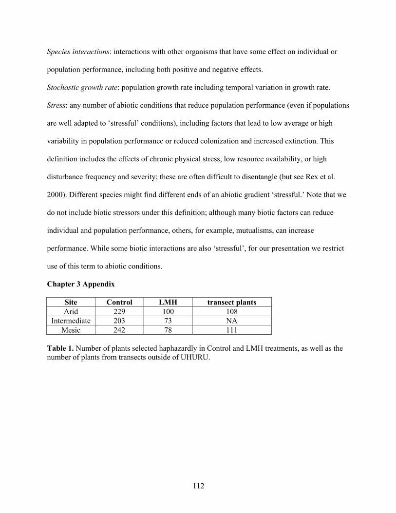
112

Species interactions: interactions with other organisms that have some effect on individual or

population performance, including both positive and negative effects.

Stochastic growth rate: population growth rate including temporal variation in growth rate.

Stress: any number of abiotic conditions that reduce population performance (even if populations

are well adapted to ‘stressful’ conditions), including factors that lead to low average or high

variability in population performance or reduced colonization and increased extinction. This

definition includes the effects of chronic physical stress, low resource availability, or high

disturbance frequency and severity; these are often difficult to disentangle (but see Rex et al.

2000). Different species might find different ends of an abiotic gradient ‘stressful.’ Note that we

do not include biotic stressors under this definition; although many biotic factors can reduce

individual and population performance, others, for example, mutualisms, can increase

performance. While some biotic interactions are also ‘stressful’, for our presentation we restrict

use of this term to abiotic conditions.

Chapter 3 Appendix

Site Control LMH transect plants Arid 229 100 108

Intermediate 203 73 NA Mesic 242 78 111

Table 1. Number of plants selected haphazardly in Control and LMH treatments, as well as the number of plants from transects outside of UHURU.

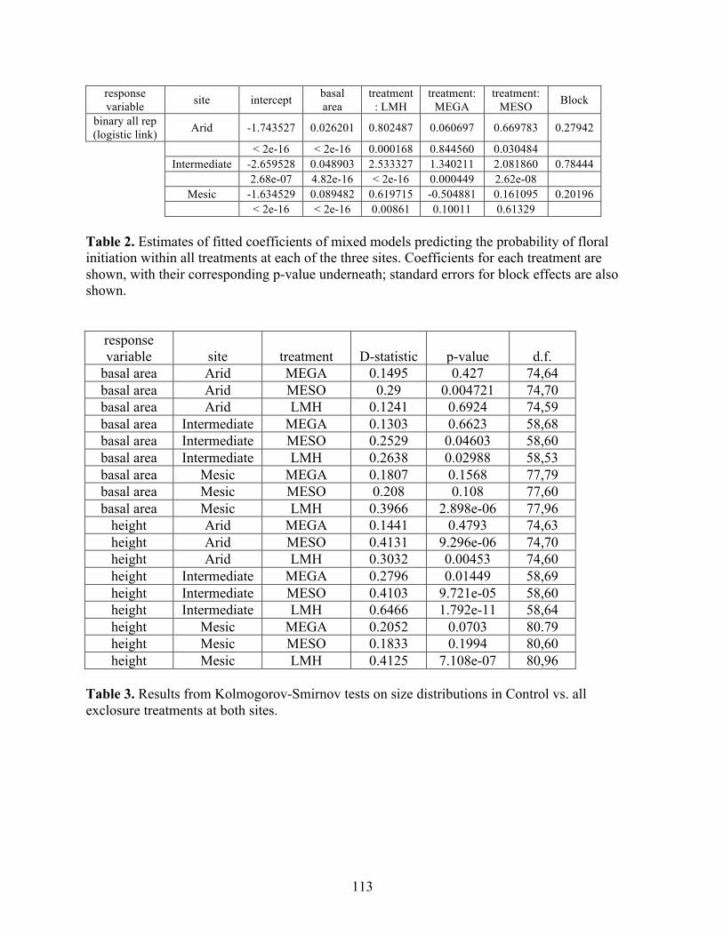
113

response variable site intercept basal

area treatment

: LMH treatment:

MEGA treatment:

MESO Block

binary all rep (logistic link) Arid -1.743527 0.026201 0.802487 0.060697 0.669783 0.27942

< 2e-16 < 2e-16 0.000168 0.844560 0.030484 Intermediate -2.659528 0.048903 2.533327 1.340211 2.081860 0.78444 2.68e-07 4.82e-16 < 2e-16 0.000449 2.62e-08 Mesic -1.634529 0.089482 0.619715 -0.504881 0.161095 0.20196 < 2e-16 < 2e-16 0.00861 0.10011 0.61329

Table 2. Estimates of fitted coefficients of mixed models predicting the probability of floral initiation within all treatments at each of the three sites. Coefficients for each treatment are shown, with their corresponding p-value underneath; standard errors for block effects are also shown.

response variable site treatment D-statistic p-value d.f.

basal area Arid MEGA 0.1495 0.427 74,64 basal area Arid MESO 0.29 0.004721 74,70 basal area Arid LMH 0.1241 0.6924 74,59 basal area Intermediate MEGA 0.1303 0.6623 58,68 basal area Intermediate MESO 0.2529 0.04603 58,60 basal area Intermediate LMH 0.2638 0.02988 58,53 basal area Mesic MEGA 0.1807 0.1568 77,79 basal area Mesic MESO 0.208 0.108 77,60 basal area Mesic LMH 0.3966 2.898e-06 77,96

height Arid MEGA 0.1441 0.4793 74,63 height Arid MESO 0.4131 9.296e-06 74,70 height Arid LMH 0.3032 0.00453 74,60 height Intermediate MEGA 0.2796 0.01449 58,69 height Intermediate MESO 0.4103 9.721e-05 58,60 height Intermediate LMH 0.6466 1.792e-11 58,64 height Mesic MEGA 0.2052 0.0703 80.79 height Mesic MESO 0.1833 0.1994 80,60 height Mesic LMH 0.4125 7.108e-07 80,96

Table 3. Results from Kolmogorov-Smirnov tests on size distributions in Control vs. all exclosure treatments at both sites.

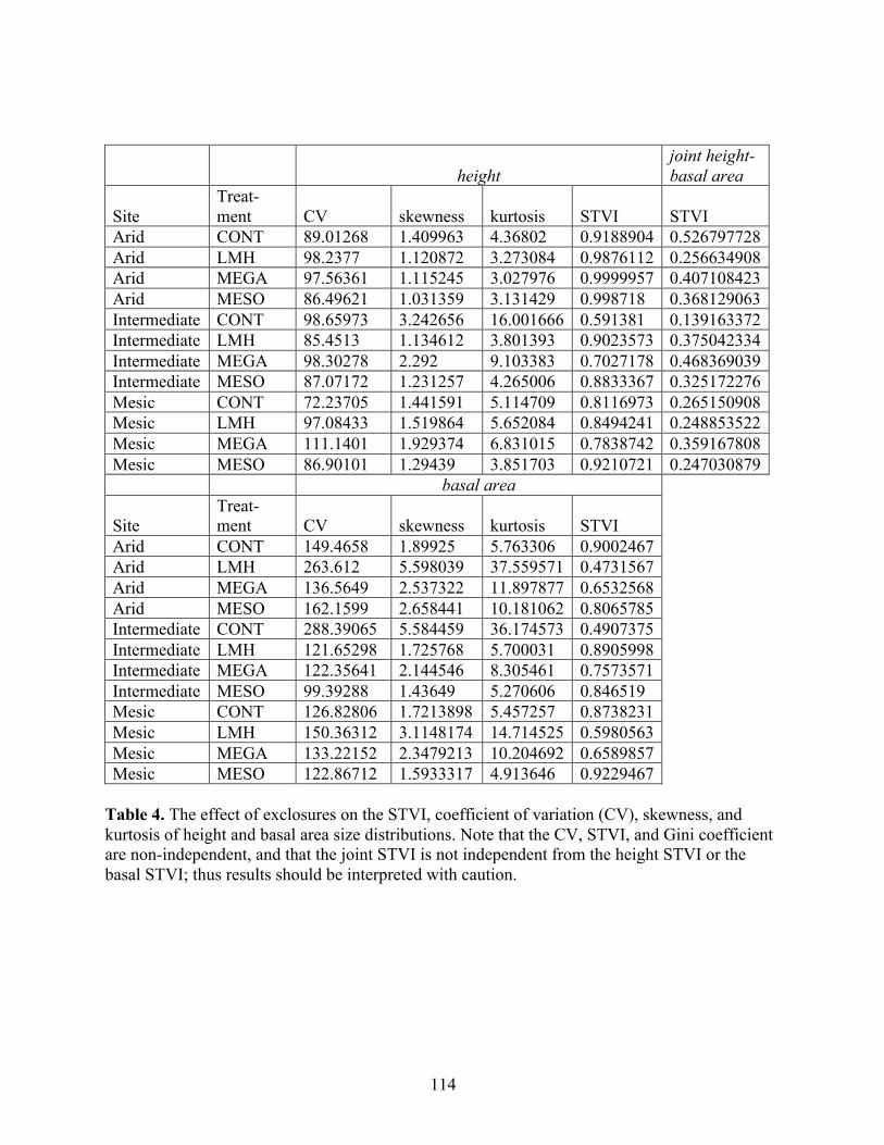
114

height joint height-basal area

Site Treat-ment CV skewness kurtosis STVI STVI

Arid CONT 89.01268 1.409963 4.36802 0.9188904 0.526797728 Arid LMH 98.2377 1.120872 3.273084 0.9876112 0.256634908 Arid MEGA 97.56361 1.115245 3.027976 0.9999957 0.407108423 Arid MESO 86.49621 1.031359 3.131429 0.998718 0.368129063 Intermediate CONT 98.65973 3.242656 16.001666 0.591381 0.139163372 Intermediate LMH 85.4513 1.134612 3.801393 0.9023573 0.375042334 Intermediate MEGA 98.30278 2.292 9.103383 0.7027178 0.468369039 Intermediate MESO 87.07172 1.231257 4.265006 0.8833367 0.325172276 Mesic CONT 72.23705 1.441591 5.114709 0.8116973 0.265150908 Mesic LMH 97.08433 1.519864 5.652084 0.8494241 0.248853522 Mesic MEGA 111.1401 1.929374 6.831015 0.7838742 0.359167808 Mesic MESO 86.90101 1.29439 3.851703 0.9210721 0.247030879 basal area

Site Treat-ment CV skewness kurtosis STVI

Arid CONT 149.4658 1.89925 5.763306 0.9002467 Arid LMH 263.612 5.598039 37.559571 0.4731567 Arid MEGA 136.5649 2.537322 11.897877 0.6532568 Arid MESO 162.1599 2.658441 10.181062 0.8065785 Intermediate CONT 288.39065 5.584459 36.174573 0.4907375 Intermediate LMH 121.65298 1.725768 5.700031 0.8905998 Intermediate MEGA 122.35641 2.144546 8.305461 0.7573571 Intermediate MESO 99.39288 1.43649 5.270606 0.846519 Mesic CONT 126.82806 1.7213898 5.457257 0.8738231 Mesic LMH 150.36312 3.1148174 14.714525 0.5980563 Mesic MEGA 133.22152 2.3479213 10.204692 0.6589857 Mesic MESO 122.86712 1.5933317 4.913646 0.9229467

Table 4. The effect of exclosures on the STVI, coefficient of variation (CV), skewness, and kurtosis of height and basal area size distributions. Note that the CV, STVI, and Gini coefficient are non-independent, and that the joint STVI is not independent from the height STVI or the basal STVI; thus results should be interpreted with caution.

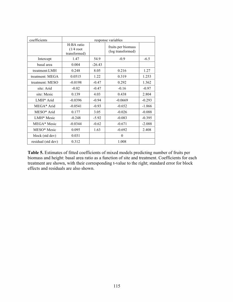
115

coefficients response variables

H:BA ratio

(1/4 root transformed)

fruits per biomass (log transformed)

Intercept 1.47 54.9 -0.9 -6.5 basal area 0.004 -26.43

treatment:LMH 0.248 8.05 0.216 1.27 treatment: MEGA 0.0515 1.22 0.319 1.253 treatment: MESO -0.0198 -0.47 0.292 1.362

site: Arid -0.02 -0.47 -0.16 -0.97 site: Mesic 0.139 4.03 0.438 2.804 LMH* Arid -0.0396 -0.94 -0.0669 -0.293

MEGA* Arid -0.0541 -0.93 -0.652 -1.866 MESO* Arid 0.177 3.05 -0.026 -0.088 LMH* Mesic -0.248 -5.92 -0.083 -0.395

MEGA* Mesic -0.0344 -0.62 -0.671 -2.088 MESO* Mesic 0.095 1.63 -0.692 2.408 block (std dev) 0.031 0

residual (std dev) 0.312 1.008 Table 5. Estimates of fitted coefficients of mixed models predicting number of fruits per biomass and height: basal area ratio as a function of site and treatment. Coefficients for each treatment are shown, with their corresponding t-value to the right; standard error for block effects and residuals are also shown.

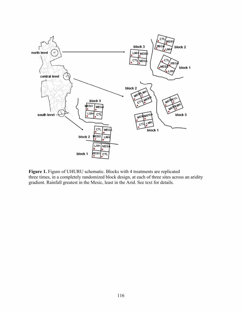
116

Figure 1. Figure of UHURU schematic. Blocks with 4 treatments are replicated three times, in a completely randomized block design, at each of three sites across an aridity gradient. Rainfall greatest in the Mesic, least in the Arid. See text for details.

117

Figure 2. Empirical CDFS constructed with raw numbers rather than proportion of the population, for both basal area and height CDFs in all site- treatment combinations. Colours as in previous figures.

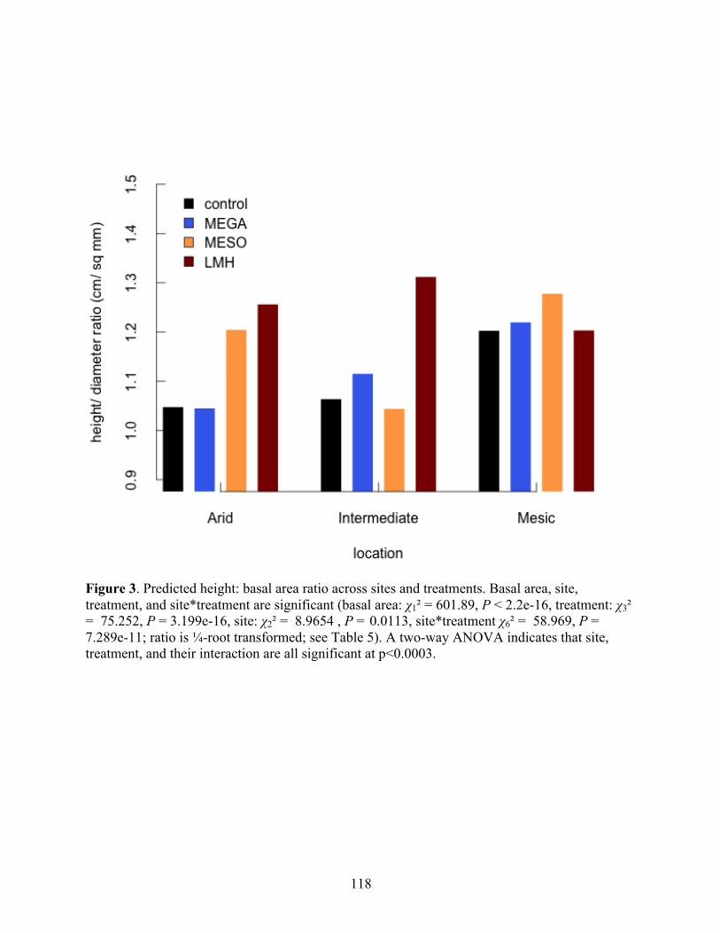
118

Figure 3. Predicted height: basal area ratio across sites and treatments. Basal area, site, treatment, and site*treatment are significant (basal area: χ1² = 601.89, P < 2.2e-16, treatment: χ3² = 75.252, P = 3.199e-16, site: χ2² = 8.9654 , P = 0.0113, site*treatment χ6² = 58.969, P = 7.289e-11; ratio is ¼-root transformed; see Table 5). A two-way ANOVA indicates that site, treatment, and their interaction are all significant at p<0.0003.

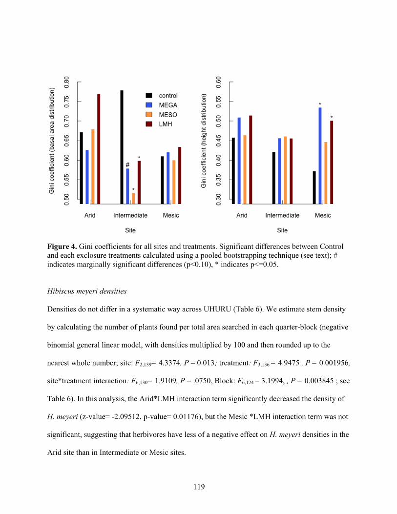
119

Figure 4. Gini coefficients for all sites and treatments. Significant differences between Control and each exclosure treatments calculated using a pooled bootstrapping technique (see text); # indicates marginally significant differences (p<0.10), * indicates p<=0.05. Hibiscus meyeri densities

Densities do not differ in a systematic way across UHURU (Table 6). We estimate stem density

by calculating the number of plants found per total area searched in each quarter-block (negative

binomial general linear model, with densities multiplied by 100 and then rounded up to the

nearest whole number; site: F2,139= 4.3374, P = 0.013; treatment: F3,136 = 4.9475 , P = 0.001956,

site*treatment interaction: F6,130= 1.9109, P = .0750, Block: F6,124 = 3.1994, , P = 0.003845 ; see

Table 6). In this analysis, the Arid*LMH interaction term significantly decreased the density of

H. meyeri (z-value= -2.09512, p-value= 0.01176), but the Mesic *LMH interaction term was not

significant, suggesting that herbivores have less of a negative effect on H. meyeri densities in the

Arid site than in Intermediate or Mesic sites.

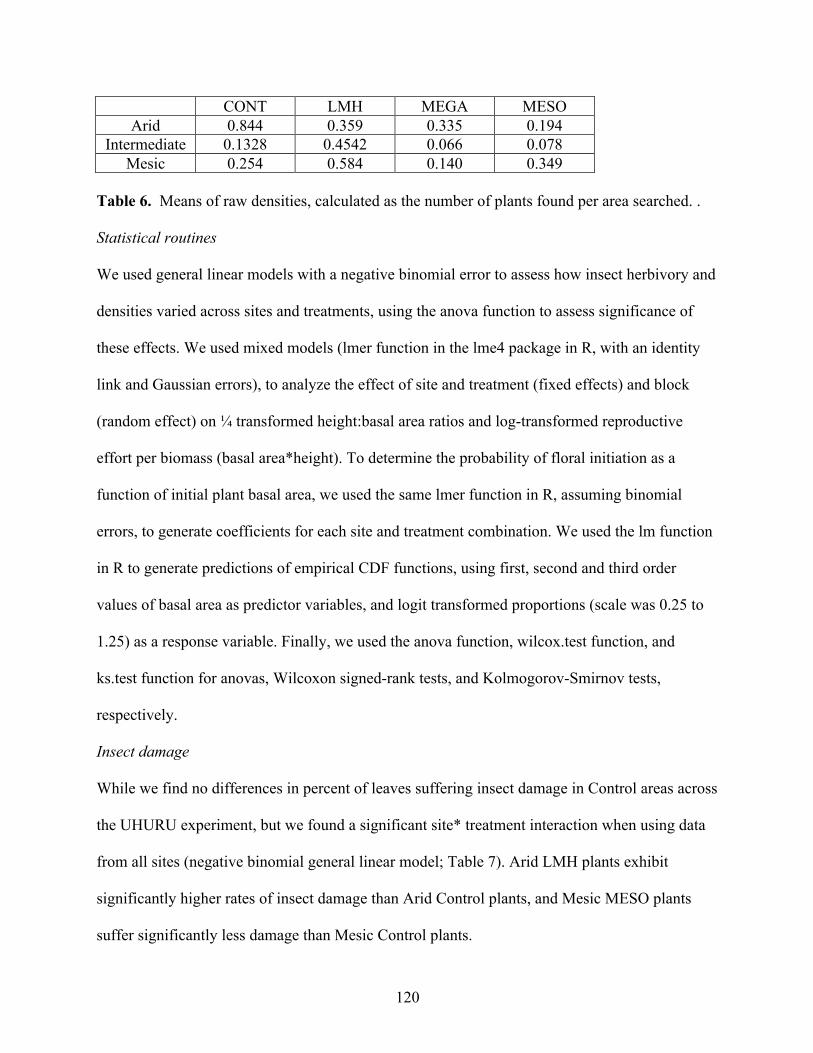
120

CONT LMH MEGA MESO Arid 0.844 0.359 0.335 0.194

Intermediate 0.1328 0.4542 0.066 0.078 Mesic 0.254 0.584 0.140 0.349

Table 6. Means of raw densities, calculated as the number of plants found per area searched. . Statistical routines

We used general linear models with a negative binomial error to assess how insect herbivory and

densities varied across sites and treatments, using the anova function to assess significance of

these effects. We used mixed models (lmer function in the lme4 package in R, with an identity

link and Gaussian errors), to analyze the effect of site and treatment (fixed effects) and block

(random effect) on ¼ transformed height:basal area ratios and log-transformed reproductive

effort per biomass (basal area*height). To determine the probability of floral initiation as a

function of initial plant basal area, we used the same lmer function in R, assuming binomial

errors, to generate coefficients for each site and treatment combination. We used the lm function

in R to generate predictions of empirical CDF functions, using first, second and third order

values of basal area as predictor variables, and logit transformed proportions (scale was 0.25 to

1.25) as a response variable. Finally, we used the anova function, wilcox.test function, and

ks.test function for anovas, Wilcoxon signed-rank tests, and Kolmogorov-Smirnov tests,

respectively.

Insect damage

While we find no differences in percent of leaves suffering insect damage in Control areas across

the UHURU experiment, but we found a significant site* treatment interaction when using data

from all sites (negative binomial general linear model; Table 7). Arid LMH plants exhibit

significantly higher rates of insect damage than Arid Control plants, and Mesic MESO plants

suffer significantly less damage than Mesic Control plants.

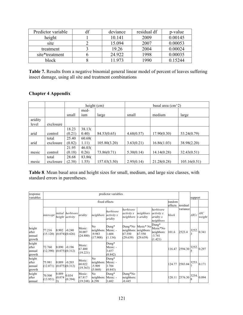
121

Predictor variable df deviance residual df p-value height 1 10.141 2009 0.00145

site 2 15.094 2007 0.00053 treatment 3 19.26 2004 0.00024

site*treatment 6 24.922 1998 0.00035 block 8 11.973 1990 0.15244

Table 7. Results from a negative binomial general linear model of percent of leaves suffering insect damage, using all site and treatment combinations

Chapter 4 Appendix

height (cm) basal area (cm^2)

small

med-ium large small medium large

aridity level exclosure

arid control

18.23(0.21)

38.13(0.40) 84.53(0.65) 4.68(0.57) 17.90(0.30) 53.24(0.79)

arid total exclosure

25.40(0.82)

60.68(1.11) 105.80(3.20) 3.63(0.21) 16.86(1.03) 38.98(2.20)

mesic control 21.95(0.18)

46.03(0.26) 73.86(0.71) 5.30(0.14) 14.14(0.28) 32.43(0.51)

mesic total exclosure

28.68(2.38)

83.86(1.55) 157.03(3.50) 2.95(0.14) 21.28(0.28) 105.16(0.51)

Table 8. Mean basal area and height sizes for small, medium, and large size classes, with standard errors in parentheses.

response variables

predictor variables

residual variance

support

fixed effects random

effects

intercept initial height

herbivore activity aridity neighbors

herbivore activity x aridity

herbivore activity x neighbors

neighbors x aridity

herbivore activity x aridity x neighbors

block AICc AIC weight

height after annual growth

77.216 (15.120)

0.902 (0.074)

-0.240 (0.426)

Mesic: 30.007 (24.880)

No neighbors: -9.983 (17.908)

Dung* Mesic: -1.604 (1.134)

Dung*No neighbors: 67.550 (29.639)

Mesic* No neighbors: 67.550 (29.639)

Dung* Mesic*No neighbors: -3.741 (1.421)

101.6 2523.4 3252.3 0.341

height after annual growth

72.760 (12.390)

0.890 (0.075)

-0.196 (0.312)

Mesic: 67.400 (19.221)

Dung* Mesic: -3.657 (0.842)

116.47 2594.30 3252.5 0.297

height after annual growth

75.981 (12.871)

0.889 (0.075)

-0.203 (0.312)

Mesic: 68.022 (19.363)

No neighbors: -5.909 (5.868)

Dung* Mesic: -3.704 (0.843)

124.77 2583.04 3253.7 0.171

height after annual

70.500 (13.951)

0.889 (0.0743)

0.034 (0.394)

Mesic: 67.817 (19.248)

No neighbors: 4.298

Dung* Mesic: -3.682

Dung*No neighbors: -0.445

120.11 2576.30 3254.8 0.094

122

growth (12.026) (0.841) (0.458)

annual survival

2.850 (0.249)

0 1 135.9 0.15

annual survival

2.619 (0.312)

No neighbors: 0.552 (0.521)

0 1 136.8 0.097

annual survival

1.964 (0.807) 0.016

( 0.027)

Mesic: -2.590 (1.472)

No neighbors: 1.574 (1.586)

Dung* Mesic: 0.293 (0.140)

Dung*No neighbors: -0.026 (0.0480)

Mesic* No neighbors: 5.027 (3.324)

Dung* Mesic*No neighbors: -0.429 (0.188)

0 1 137 0.087

annual p(fruit)

0.774 (0.327)

0.018 (0.005)

Mesic: -0.852 (0.357)

0.056 1 292.1 0.263

annual p(fruit)

1.288 (0.593)

0.017 (0.005)

-0.016 (0.016)

Mesic: -1.036 (0.380)

0.029 1 -141.438

293.1

annual p(fruit)

0.843 (0.356)

0.018 (0.005)

Mesic: -0.855 (0.355)

No neighbors: -0.147 (0.295)

0.054 1 -141.843

293.9

annual p(fruit)

0.380 (0.324)

0.018 (0.005) 0.226 1

-143.987

294.1

annual number of fruits | fruiting

1.702 (0.242)

0.010 (0.002)

-0.017 (0.006)

Mesic: -0.544 (0.161)

0 1.466 904.3 0.187

annual number of fruits | fruiting

1.443 (0.285)

0.010 (0.002)

-0.008 (0.009)

Mesic: -0.534 (0.161)

No neighbors: 0.504 (0.299)

Dung * no neighbors: -0.018 (0.011)

3.33E-12

1.450e+00

-444.527

905.6

annual number of fruits | fruiting

1.661 (0.252)

0.010 (0.002)

-0.017 (0.006)

Mesic: -0.542 (0.161)

No neighbors: 0.085 (0.146)

0 1.4637 -445.811

906.0

annual number of fruits | fruiting

1.271 (0.314)

0.010 (0.002)

-0.004 (0.009)

Mesic: -0.332 (0.224)

No neighbors: 0.863 (0.408)

Dung* no neighbors: -0.025 (0.013)

Mesic *no neighbors: -0.413 (0.321)

6.1974e-13

1.4416e+00

-443.705

906.1

annual number of fruits | fruiting

1.698 (0.245)

0.010 (0.002)

-0.017 (0.007)

Mesic: -0.507 (0.390)

Dung * Mesic: -0.002 (0.019)

0 1.4655 -445.976

906.4

Table 9. Best-fit models (AIC weight >0.08) of vital rates as a function of height, herbivore presence, aridity, and neighbor presence. Parameter estimates for coefficients for main effects are shown, with standard errors in parentheses and MCMC estimates of p-values in italics; for categorical or interaction effects, each parameter estimate is shown separately. Variance of random effects and residual variance are also shown; for binomial mixed models, residual variance is fixed at 1. We do not present significance values for individual parameters, as their interpretation for mixed models is not straightforward (Golderg et al. 1999).

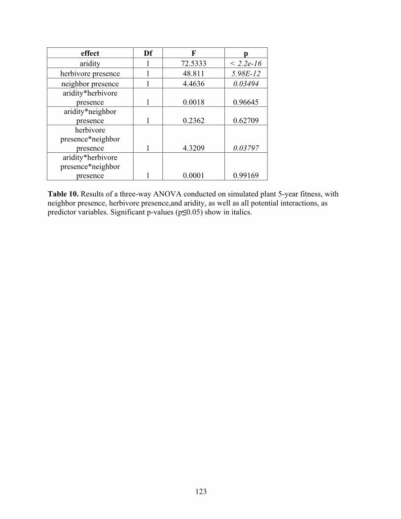
123

effect Df F p aridity 1 72.5333 < 2.2e-16

herbivore presence 1 48.811 5.98E-12 neighbor presence 1 4.4636 0.03494 aridity*herbivore

presence 1 0.0018 0.96645 aridity*neighbor

presence 1 0.2362 0.62709 herbivore

presence*neighbor presence 1 4.3209 0.03797

aridity*herbivore presence*neighbor

presence 1 0.0001 0.99169 Table 10. Results of a three-way ANOVA conducted on simulated plant 5-year fitness, with neighbor presence, herbivore presence,and aridity, as well as all potential interactions, as predictor variables. Significant p-values (p≤0.05) show in italics.

124

Figure 5. Best fit mixed-model predictions of survival, probability of fruiting, and number of fruits given fruiting, as a function of neighbor presence, aridity, and herbivore presence (zero herbivore activity, A, C, E, and average herbivore activity across control treatments, B, D, F). Bars represent standard error of fixed-effect parameter estimates.

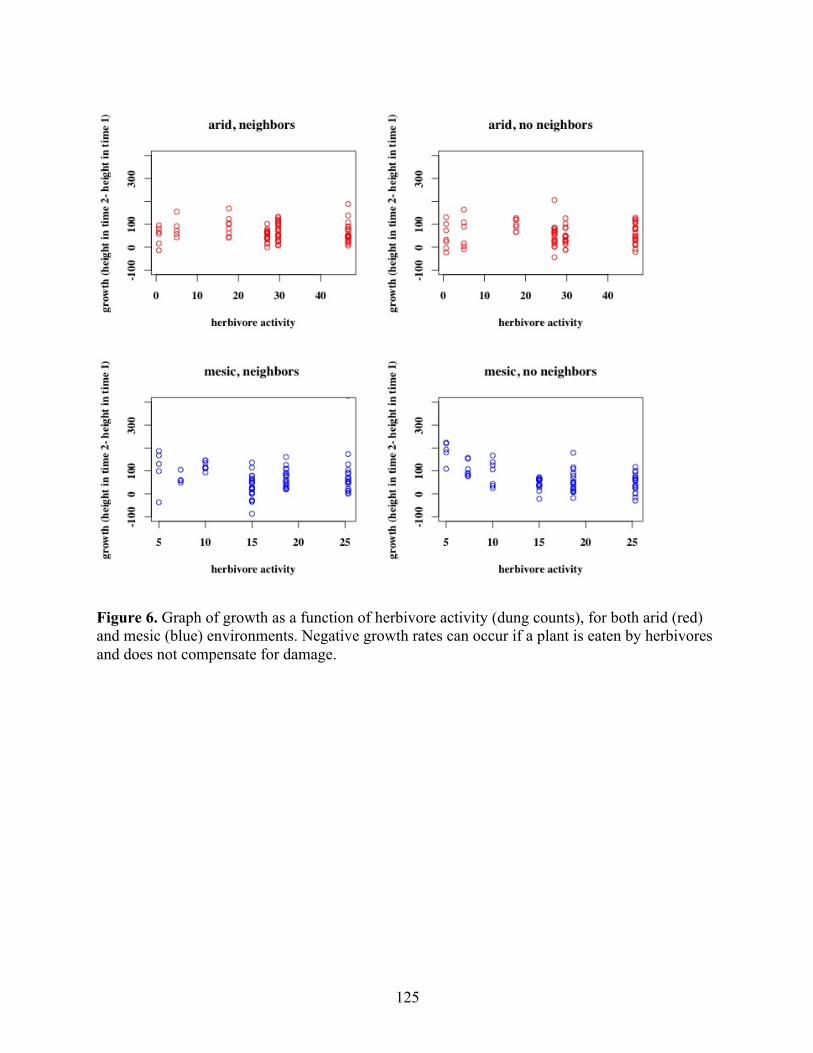
125

Figure 6. Graph of growth as a function of herbivore activity (dung counts), for both arid (red) and mesic (blue) environments. Negative growth rates can occur if a plant is eaten by herbivores and does not compensate for damage.

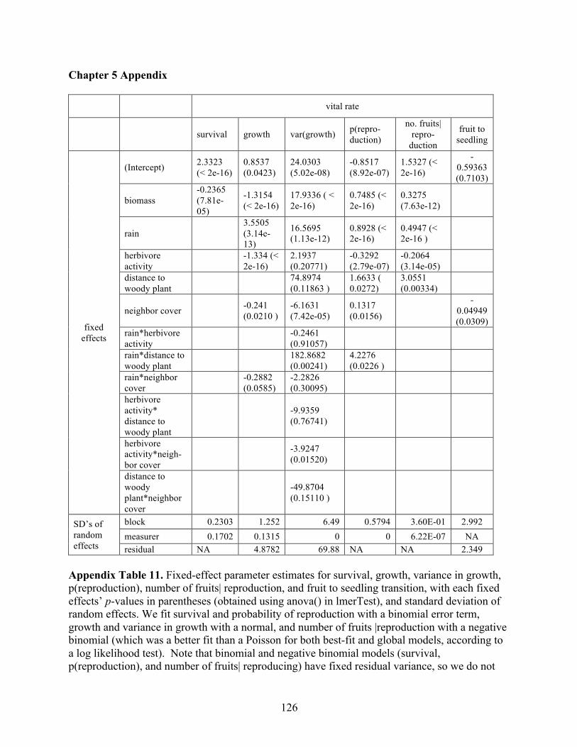
126

Chapter 5 Appendix

vital rate

survival growth var(growth) p(repro-duction)

no. fruits| repro-

duction

fruit to seedling

fixed effects

(Intercept) 2.3323 (< 2e-16)

0.8537 (0.0423)

24.0303 (5.02e-08)

-0.8517 (8.92e-07)

1.5327 (< 2e-16)

-0.59363 (0.7103)

biomass -0.2365 (7.81e-05)

-1.3154 (< 2e-16)

17.9336 ( < 2e-16)

0.7485 (< 2e-16)

0.3275 (7.63e-12)

rain

3.5505 (3.14e-13)

16.5695 (1.13e-12)

0.8928 (< 2e-16)

0.4947 (< 2e-16 )

herbivore activity

-1.334 (< 2e-16)

2.1937 (0.20771)

-0.3292 (2.79e-07)

-0.2064 (3.14e-05)

distance to woody plant

74.8974 (0.11863 )

1.6633 ( 0.0272)

3.0551 (0.00334)

neighbor cover

-0.241 (0.0210 )

-6.1631 (7.42e-05)

0.1317 (0.0156)

-0.04949 (0.0309)

rain*herbivore activity

-0.2461 (0.91057)

rain*distance to woody plant

182.8682 (0.00241)

4.2276 (0.0226 )

rain*neighbor cover

-0.2882 (0.0585)

-2.2826 (0.30095)

herbivore activity* distance to woody plant

-9.9359 (0.76741)

herbivore activity*neigh-bor cover

-3.9247 (0.01520)

distance to woody plant*neighbor cover

-49.8704 (0.15110 )

SD’s of random effects

block 0.2303 1.252 6.49 0.5794 3.60E-01 2.992 measurer 0.1702 0.1315 0 0 6.22E-07 NA residual NA 4.8782 69.88 NA NA 2.349

Appendix Table 11. Fixed-effect parameter estimates for survival, growth, variance in growth, p(reproduction), number of fruits| reproduction, and fruit to seedling transition, with each fixed effects’ p-values in parentheses (obtained using anova() in lmerTest), and standard deviation of random effects. We fit survival and probability of reproduction with a binomial error term, growth and variance in growth with a normal, and number of fruits |reproduction with a negative binomial (which was a better fit than a Poisson for both best-fit and global models, according to a log likelihood test). Note that binomial and negative binomial models (survival, p(reproduction), and number of fruits| reproducing) have fixed residual variance, so we do not

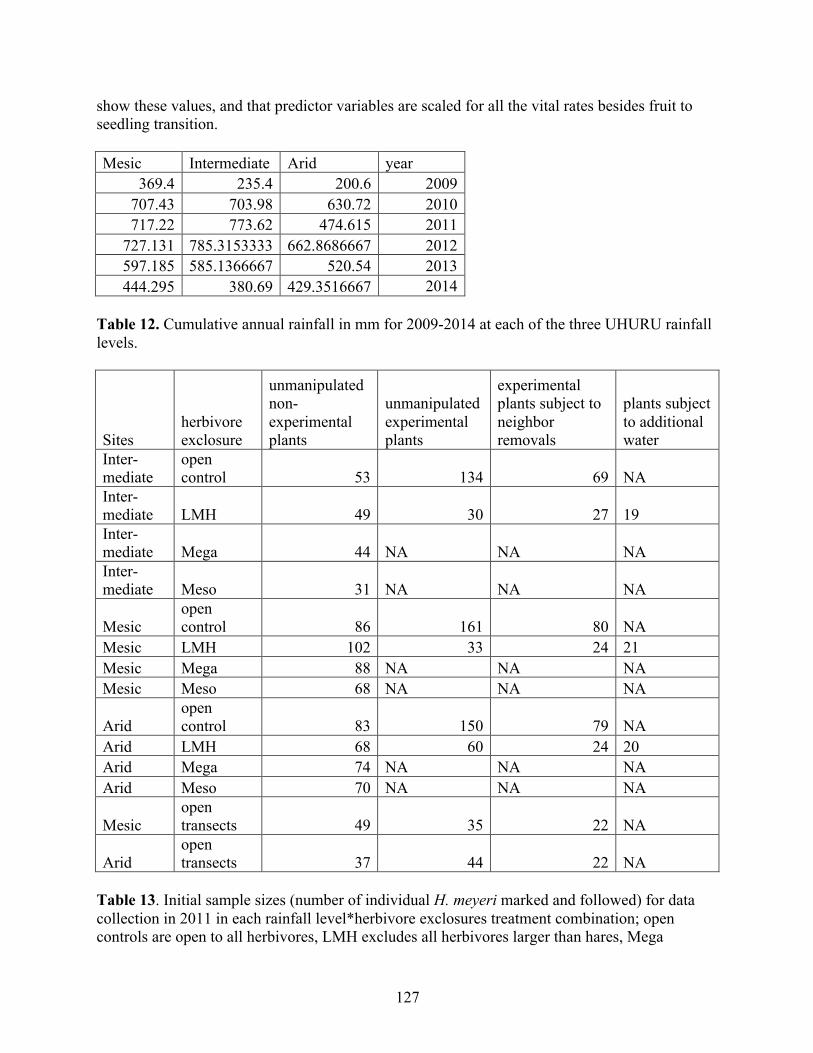
127

show these values, and that predictor variables are scaled for all the vital rates besides fruit to seedling transition. Mesic Intermediate Arid year

369.4 235.4 200.6 2009 707.43 703.98 630.72 2010 717.22 773.62 474.615 2011

727.131 785.3153333 662.8686667 2012 597.185 585.1366667 520.54 2013 444.295 380.69 429.3516667 2014

Table 12. Cumulative annual rainfall in mm for 2009-2014 at each of the three UHURU rainfall levels.

Sites herbivore exclosure

unmanipulated non-experimental plants

unmanipulated experimental plants

experimental plants subject to neighbor removals

plants subject to additional water

Inter-mediate

open control 53 134 69 NA

Inter-mediate LMH 49 30 27 19 Inter-mediate Mega 44 NA NA NA Inter-mediate Meso 31 NA NA NA

Mesic open control 86 161 80 NA

Mesic LMH 102 33 24 21 Mesic Mega 88 NA NA NA Mesic Meso 68 NA NA NA

Arid open control 83 150 79 NA

Arid LMH 68 60 24 20 Arid Mega 74 NA NA NA Arid Meso 70 NA NA NA

Mesic open transects 49 35 22 NA

Arid open transects 37 44 22 NA

Table 13. Initial sample sizes (number of individual H. meyeri marked and followed) for data collection in 2011 in each rainfall level*herbivore exclosures treatment combination; open controls are open to all herbivores, LMH excludes all herbivores larger than hares, Mega

128

excludes mega-herbivores and larger, and Meso excludes meso-herbivores and larger. At each census, we replaced plants as necessary to maintain consistent sample sizes; plants were lost due to mortality or inability to relocate plants. For our experimental work, we tagged more plants in control plots than we did in herbivore exclosure plots (due to a desire to leave some plants in herbivore exclosures unmanipulated for future experiments). Further, in LMH plots, experimental plants were 1/3 control, 1/3 neighbor removal, and 1/3 supplemental water, while in control plots, experimental plants were 1/3 neighbor removal plants and 2/3 control, with no supplemental watering (a pilot experiment indicated that elephants preferentially consume supplementally watered plants, so we did not conduct this experiment in the open control).

Interaction

Total ∆∆𝜆 Density ∆∆𝜆 Life history ∆∆𝜆

Per capita ∆∆𝜆

Total ∆∆𝜆 (non-specific predictors)

neighbors -1.725 -0.02110436 -1.203694 -0.0320246 -1.213367

herbivory -1.461 0.08938248 -0.9333092

-0.0004559

387 -0.7433832

pollination 0.1744 0 0.1151085 0.005195311 0.1247737

Interaction

Total ∆∆𝜆

Sur-vival ∆∆𝜆

growth ∆∆𝜆

Var(gr) ∆∆𝜆

P(rep) ∆∆𝜆

No seeds |repro-duction ∆∆𝜆

Fruit-to-seed-ling ∆∆𝜆

Total ∆∆𝜆 (non-specific predictors)

neighbors

-1.725

-0.021758

57

-0.01452455

-0.0396728

4

0.01431554

0.04155432

-1.50182843

-1.213367

herbivory -1.461

0.088153

62

0.08646560

0.072363

0.08099107

0.1321458

-0.83239250

-0.7433832

pollination

0.1744 5.889145e-05

-3.546622e-04

0.001502456

-0.00396262

3

-0.006100006

1.559514e-01 0.1247737

Table 14. ∆∆𝜆 values for each interaction and the contribution of each type of mechanism and vital rate to total ∆∆𝜆. Note that the Total ∆∆𝜆 (non-specific predictors) sets all other species interactions to the mean value between the Arid and Mesic Sites (e.g., for neighbors, herbivore activity is the mean herbivore activity in the Mesic and Arid Sites’ full herbivore exclosures, pollinator density is zero, and distance to woody plant is the mean distance in the Mesic and Arid Sites’ full exclosures; see Chapter 5), so is not the same as the Total ∆∆𝜆, which uses Site-specific species interactions values, such that Arid Site values are different than Mesic Site values. “Total ∆∆𝜆” is the value used in Chapter 5 Figure 1.

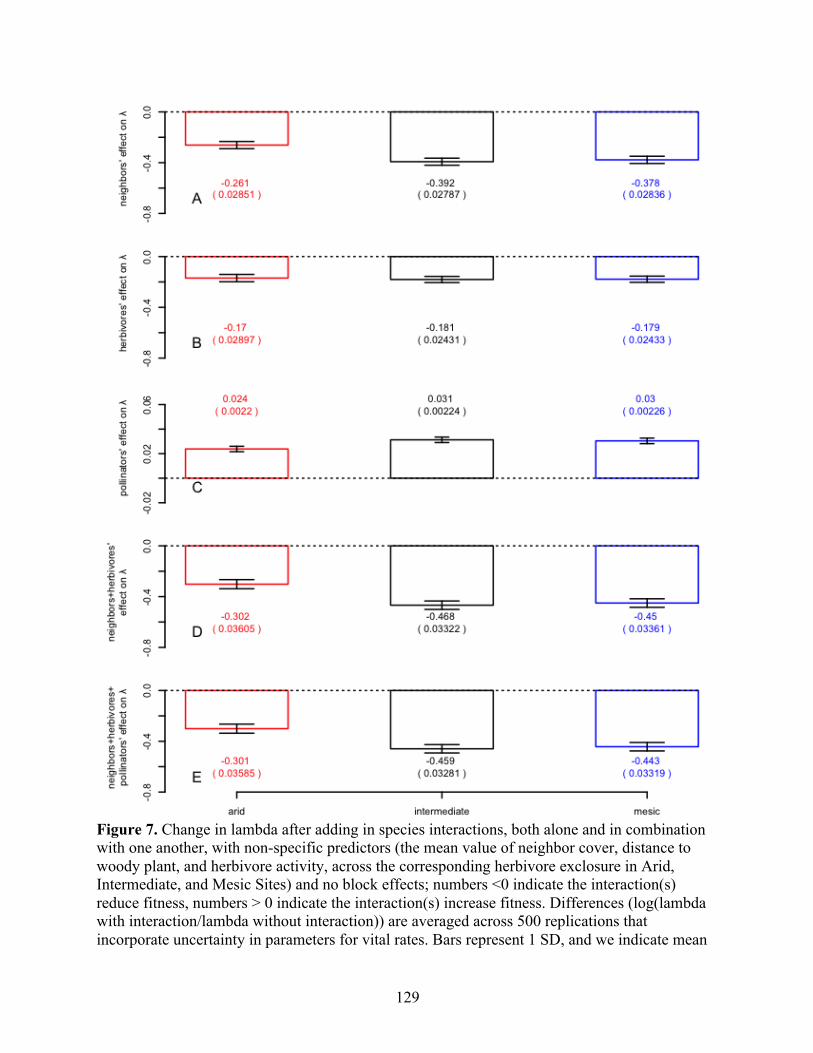
129

Figure 7. Change in lambda after adding in species interactions, both alone and in combination with one another, with non-specific predictors (the mean value of neighbor cover, distance to woody plant, and herbivore activity, across the corresponding herbivore exclosure in Arid, Intermediate, and Mesic Sites) and no block effects; numbers <0 indicate the interaction(s) reduce fitness, numbers > 0 indicate the interaction(s) increase fitness. Differences (log(lambda with interaction/lambda without interaction)) are averaged across 500 replications that incorporate uncertainty in parameters for vital rates. Bars represent 1 SD, and we indicate mean

130

change in lambda (with standard errors in parentheses) because differences are difficult to see. Note that the similarity between this figure and Chapter 5 Fig. 1 suggest that density exerts minimal effects on the overall magnitude of the change in lambda between Mesic and Arid Sites, as our main text analyses also indicate. Analogous values for predictions using global models for vital rates are neighbors: Arid Site: -0.288 (SE: 0.04), Intermediate: -0.432 (0.0405), Mesic: -0.417 (0.0409), herbivores: -0.244 (0.0427), -0.262 (0.0439), -0.26 (0.0435), pollinators: 0.025 (0.0028), 0.032 (0.0027), 0.031 (0.0028), neighbors + herbivores: -0.336 (0.0471), -0.521 (0.0467), -0.502 (0.0467), neighbors+ herbivores+ pollinators: -0.334 (0.047), -0.459 (0.0328), -0.443 (0.0332).

Figure 8. Sensitivities of lambda to size-specific vital rates at Arid and Mesic Sites. Results are shown for matrices with no species interactions and Site-specific values of distance to woody

131

plant (as in the reference matrix in Chapter 5, Fig. 1). Sensitivities were obtained via perturbation. Note the change in scale between growth, variance in growth, and number of fruits given reproduction.

Pollinator effects

Hibiscus meyeri has a floral phenotype that appears to favor outcrossing by an insect vector, but

presumably assures self-fertilization in the absence of an effective pollination event. Similar to a

well-studied Hibiscus in this same system (Ruiz-Guajardo 2008), H. meyeri displays flowers for

only one day; stigmas remain exposed to outcross pollen until the afternoon, when, if they have

not received outcross pollen, they bend back to touch their style to the anthers surrounding the

style (presumably resulting in self-pollination; A. Louthan, pers. obs). Hibiscus trionum, a

facultative selfer with a similar floral phenotype to H. meyeri, shows weak, delayed inbreeding

depression, likely due to repeated incidences of self-fertilization. In H. trionun, performance of

selfers compared to outcrosses was worst for maternal seeds per fruit (outcross to selfer

performance ratio= 1.0526) and flowers per plant in the F1 generation (ratio=1.0989) (Seed,

Vaughton, and Ramsey 2006).

We opportunistically collected data on fraction of self-pollinated flowers in 245 plants

across all levels and treatments from 2010 to 2013. Fraction of self-pollinated flowers per plant

in the field ranges from 0 to 1, but there is little variation among levels in per plant average

selfing rate across flowers (Arid Site 0.99, Intermediate, 0.99, Mesic, 1.0); note that

incorporating lower selfing rates in Arid Sites into our analysis would result in even weaker

effects of pollinators in Arid Sites.

Most commonly, plants self-pollinate all their flowers, but some plants receive outcross

pollen on all their flowers (Fig. 9). Thus, we assumed that all observed H. meyeri plants selfed in

the field, and for our pollination treatment, we simulated outcrossing of all flowers by adding a

132

fractional increase of 1.0526 in seeds per fruit and a fractional increase in 1.0989 in fruits per

plant. Thus, our “pollinator” treatment represents the most optimistic gains possible in pollinator

service: complete selfing to complete outcrossing, but these are both realistic possibilities in the

field.

Figure 9. Fraction of selfed flowers on a plant (where a style recurved more than 90 degrees counted as a selfed flower) across all levels and treatments.

Another possible complication to our way of simulating pollination effects is that effects

of inbreeding depression are usually more severe in stressful environments (Armbruster & Reed

2005). Thus, a change from 0 to 100% outcross pollination may have more substantial impacts in

our Arid Site than in our Mesic Site. When incorporating a 69% increase in the magnitude of

inbreeding depression in the Arid Site compared to the Mesic Site (species-wide average of

increase in inbreeding depression in stressful v. benign sites, according to a recent review,

Armbruster & Reed 2005), we see stronger effects of pollinators in our Arid Site (completely

contrary to SIASH). It is possible that this percentage is an overestimation of the magnitude of

effects of inbreeding depression in the Arid Site in H. meyeri, for three reasons: (i) while some of

133

the “benign” sites in this review were greenhouse conditions, watering H. meyeri in our Mesic

Site still increases performance, indicating our Mesic Site is clearly still stressful; (ii) lineages

within an inbred population often exhibit very different relationships between stress and

inbreeding depression, suggesting inconsistent responses (Armbruster & Reed 2005); and (iii)

24% of species show no change at all in inbreeding depression with stress (Armbruster & Reed

2005).

Random effects are unimportant

We conducted replicate measurements by different measurers at the same time (or within ~2

days) to get an estimate of measurer effects on our measurement of size. Our two metrics of size,

basal area and height, were strongly correlated across multiple measurers. We assumed that

measurements by A. Louthan (who performed measurements consistently throughout the

duration of this study) were “true” measurements. Average fractional deviation from Louthan’s

measurements [(alternate measurer’s measurements- Louthan’s measurements)/Louthan’s

measurements] was small (0.14 for basal area and 0.12 for height), and the r-squared of log-

transformed basal area*height (we use basal area*height in our biomass estimation; see below)

of a linear regression between the alternate measurer’s measurements and Louthan’s

measurements was 0.93 (see Fig. 10). Further, the random effect of measurer only explained a

small fraction of total variance of the model (see Table 15).

134

Figure 10. Louthan’s measurement v. alternate measurers’ measurement of basal area*height. We expect to see more substantial variation at larger sizes, as larger plants are likely measured with more error.

vital rate model

fraction variance explained by block

fraction variance explained by measurer

survival, best fit 4.90E-02 2.68E-02 growth, best fit 6.18E-02 6.81E-04 variance in growth, best fit 8.55E-03 0.00E+00 p(reproduction), best fit 2.51E-01 0.00E+00 number of fruits|reproduction, best fit 1.15E-01 3.43E-13 survival, global 4.02E-02 2.18E-02 growth, global 5.98E-02 8.79E-04 variance in growth, global 7.52E-03 1.85E-16 p(reproduction), global 2.47E-01 0.00E+00 number of fruits|reproduction, global 1.09E-01 0.00E+00

Table 15. Fraction of total variance (residual variance + variance explained by block + variance explained by measurer) attributed to each random effect, for both best-fit and global vital rates.

135

Getting biomass

To generate a unified metric of size, we measured and harvested above-ground biomass of 30

plants arrayed equally across the three rainfall levels, drying to a constant weight and then

regressing log-transformed dry biomass on log-transformed basal area *height. This gave us

biomass= exp( 0.3338488 * log(basal area*height)), which had an r-squared of 0.88.

Plants subject to neighbor removal treatments show a different relationship between basal

area and height (increased basal area growth relative to height, perhaps due to alleviation of light

limitation; A. Louthan personal observation). To generate a separate biomass regression for

plants without neighbors, in July 2012 we also conducted neighbor removals on 19 plants using

the same protocols as neighbor removals in the main text (7 at the Intermediate site, 3 at the Arid

Site, 9 at the Mesic Site; sample sizes are unequal due to mortality after establishment of these

treatments, and for each site, we had roughly equal numbers of plants in both the full exclosures

and areas open to herbivores). In June 2014, we measured and harvested them, drying to a

constant weight and then regressing log-transformed dry biomass on log-transformed basal area

*height. This gave us biomass= exp(0.3593906 * log(basal area*height)), which had an r-

squared of 0.90. We used these two equations to get estimates of biomass for both

unmanipulated plants and plants subject to neighbor removal treatments.

Rainfall is a stressor

We know that water is a limiting resource. First, we observed the highest lambda values in the

Mesic Site in the absence of any of our three measured species interactions (Table 16). Also, we

conducted a watering experiment within the full exclosures at each of three levels, watering 19-

21 plants at each level (see Table 9 for sample sizes) with 7.5 L every month for 10 months

(March 2014-Feburary 2015) and comparing them to the growth of unmanipulated control plants

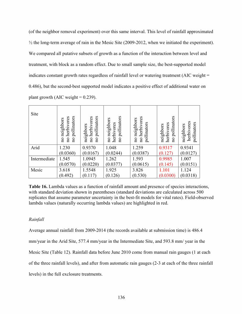
136

(of the neighbor removal experiment) over this same interval. This level of rainfall approximated

½ the long-term average of rain in the Mesic Site (2009-2012, when we initiated the experiment).

We compared all putative subsets of growth as a function of the interaction between level and

treatment, with block as a random effect. Due to small sample size, the best-supported model

indicates constant growth rates regardless of rainfall level or watering treatment (AIC weight =

0.486), but the second-best supported model indicates a positive effect of additional water on

plant growth (AIC weight = 0.239).

Site

no n

eigh

bors

no

her

bivo

res

no p

ollin

ator

s

neig

hbor

s no

her

bivo

res

no p

ollin

ator

s

no n

eigh

bors

he

rbiv

ores

no

pol

linat

ors

no n

eigh

bors

no

her

bivo

res

polli

nato

rs

neig

hbor

s he

rbiv

ores

no

pol

linat

ors

neig

hbor

s h

erbi

vore

s po

llina

tors

Arid 1.230 (0.0360)

0.9370 (0.0167)

1.048 (0.0244)

1.259 (0.0387)

0.9317 (0.127)

0.9341 (0.0127)

Intermediate 1.545 (0.0570)

1.0945 (0.0220)

1.262 (0.0377)

1.593 (0.0615)

0.9985 (0.145)

1.007 (0.0151)

Mesic 3.618 (0.492)

1.5548 (0.117)

1.925 (0.126)

3.826 (0.530)

1.101 (0.0300)

1.124 (0.0318)

Table 16. Lambda values as a function of rainfall amount and presence of species interactions, with standard deviation shown in parentheses (standard deviations are calculated across 500 replicates that assume parameter uncertainty in the best-fit models for vital rates). Field-observed lambda values (naturally occurring lambda values) are highlighted in red.

Rainfall

Average annual rainfall from 2009-2014 (the records available at submission time) is 486.4

mm/year in the Arid Site, 577.4 mm/year in the Intermediate Site, and 593.8 mm/ year in the

Mesic Site (Table 12). Rainfall data before June 2010 come from manual rain gauges (1 at each

of the three rainfall levels), and after from automatic rain gauges (2-3 at each of the three rainfall

levels) in the full exclosure treatments.

137

Calculation of rain & interactor density values

We used cumulative rainfall (the average of 2-3 automatic rain gauges at each rainfall

level) between the midpoint of the first H. meyeri remeasurement period (this period was usually

2-3 months long) and the midpoint of the second H. meyeri remeasurement period as a predictor

variable. Specifically, we used rainfall between each of our H. meyeri remeasurement periods as

a predictor variable for survival and growth during that same interval, as well as reproduction at

the end of that interval.

Similarly, we used dung counts (a proxy for herbivore activity) during the interval as a

predictor of survival and growth during that interval and reproduction at the end of that interval.

For each dung survey*rainfall level*block*treatment combination, we summed total dung counts

collected along 3 transects to get an estimate of herbivore activity per survey (Goheen et al.

2013). To obtain an estimate of average herbivore activity in each rainfall level*block*treatment

during the intervals between H. meyeri measurements, we averaged the data from the dung

counts conducted between the midpoint of the first H. meyeri remeasurement period and the

midpoint of the second H. meyeri remeasurement period. We used the midpoint of the dates over

which the dung survey was conducted as the date of the dung survey in this analysis. For our

initial measurements, we averaged the data from the dung counts collected over the previous

year. We discarded dung counts for hippo, which are only counted in 1 survey (only 1 dung pile

was found), as well as for all predators. For survey 9, the Intermediate Site blocks 1 & 2 were not

labeled, so we discarded these dung counts. For survey 8, there were missing data for a few

species (new camel dung, old waterbuck dung, baboon), so we replaced these missing data with

zeros, as average dung counts across all transects for these species were 0.004, 0.004, 0.005,

respectively.

138

For our transects outside of the UHURU plots, for which we had neither rainfall data nor

herbivore dung counts, we used the average of all that rainfall levels’ blocks’ data for a given

time period. Transects were ~200 m from the plots, and thus likely experience similar herbivore

densities and rainfall levels.

For our main results, presented in Figs. 1 and 2 of Chapter 5, we used the average of

observed rainfall values between our H. meyeri remeasurement periods to get rainfall level-

specific values of rainfall, and we averaged across all blocks’ observed herbivore activity values

between our H. meyeri remeasurement periods to get rainfall level* herbivore exclosure

treatment-specific herbivore activity predictor variables. For neighbor cover and distance to

woody plant, we averaged all non-manipulated plants’ observed values in each rainfall level*

herbivore exclosure plot to get a mean value for each rainfall level* herbivore exclosure. For our

results with non-specific predictor variables, for rainfall we used the average of observed rainfall

values between our H. meyeri remeasurement periods to get rainfall level-specific values of

rainfall (as above). For dung counts, we averaged across all blocks’ observed herbivore activity

values between our H. meyeri remeasurement periods to get herbivore exclosure treatment-

specific herbivore activity predictor variables. Finally, for neighbor cover and distance to woody

plant, we averaged all non-manipulated plants’ observed values to get a universal mean value.

For our calculations of sensitivities, we used a matrix with no neighbors, herbivores, or

pollinators, and the mean distance to woody plant (across Arid, Intermediate, and Mesic Sites) in

the absence of herbviores. We assumed that herbivore activity in full exclosures was “no

herbivory” and that a neighbor cover of 0 was “no neighbors.”

Densities of herbivores across herbivore exclosures & rainfall levels

139

Herbivore exclosures are highly effective and herbivore densities are higher in our Arid

Site. We used dung count data from the 19 dung count surveys used in this study, conducted

between July 2010 and May 2015, to test for differences in herbivore activity. We summed total

dung found in each rainfall level*treatment*block* survey combination, then averaged across

blocks for each survey. We found a significant effect of rainfall level on log-transformed dung

counts in control areas open to herbivores (ANOVA, F= 5.69 p= 0.006), with higher herbivore

activity in the Arid Site than in the Mesic Site (Tukey’s HSD, p= 0.004); mean dung counts

values in open controls are Arid Site: 23.6, Intermediate: 21.5, and Mesic: 13.4. Herbivore

exclosure had significant effects on total dung: a two-way ANOVA revealed nonsignifincant

effects of level and level*treatment, but significant effects of treatment (F=94.7488 p=<2e-16).

Control, MEGA, and MESO had greater amounts of total dung than LMH (Tukey’s HSD,

p<<0.05).

Permission to use Published works in Dissertation

140

3/5/2016 RightsLink Printable License

https://s100.copyright.com/AppDispatchServlet 1/6

ELSEVIER LICENSE

TERMS AND CONDITIONS

Mar 05, 2016

This is a License Agreement between Allison M Louthan ("You") and Elsevier ("Elsevier")provided by Copyright Clearance Center ("CCC"). The license consists of your order details,the terms and conditions provided by Elsevier, and the payment terms and conditions.

All payments must be made in full to CCC. For payment instructions, please see

information listed at the bottom of this form.

Supplier Elsevier LimitedThe Boulevard,Langford LaneKidlington,Oxford,OX5 1GB,UK

Registered CompanyNumber

1982084

Customer name Allison M Louthan

Customer address 964 Lost Angel Road

  BOULDER, CO 80302

License number 3822551416798

License date Mar 05, 2016

Licensed content publisher Elsevier

Licensed content publication Trends in Ecology & Evolution

Licensed content title Where and When do Species Interactions Set Range Limits?

Licensed content author Allison M. Louthan,Daniel F. Doak,Amy L. Angert

Licensed content date December 2015

Licensed content volumenumber

30

Licensed content issuenumber

12

Number of pages 13

Start Page 780

End Page 792

Type of Use reuse in a thesis/dissertation

Portion full article

Format print

Are you the author of thisElsevier article?

Yes

Will you be translating? No

Title of yourthesis/dissertation

THE RELATIVE STRENGTH OF ABIOTIC AND BIOTIC CONTROLS ONSPECIES RANGE LIMITS

Expected completion date Mar 2016

141

3/5/2016 RightsLink Printable License

https://s100.copyright.com/AppDispatchServlet 2/6

Estimated size (number ofpages)

150

Elsevier VAT number GB 494 6272 12

Permissions price 0.00 USD

VAT/Local Sales Tax 0.00 USD / 0.00 GBP

Total 0.00 USD

Terms and Conditions

INTRODUCTION1. The publisher for this copyrighted material is Elsevier.  By clicking "accept" inconnection with completing this licensing transaction, you agree that the following termsand conditions apply to this transaction (along with the Billing and Payment terms andconditions established by Copyright Clearance Center, Inc. ("CCC"), at the time that youopened your Rightslink account and that are available at any time athttp://myaccount.copyright.com).

GENERAL TERMS2. Elsevier hereby grants you permission to reproduce the aforementioned material subject tothe terms and conditions indicated.3. Acknowledgement: If any part of the material to be used (for example, figures) hasappeared in our publication with credit or acknowledgement to another source, permissionmust also be sought from that source.  If such permission is not obtained then that materialmay not be included in your publication/copies. Suitable acknowledgement to the sourcemust be made, either as a footnote or in a reference list at the end of your publication, asfollows:"Reprinted from Publication title, Vol /edition number, Author(s), Title of article / title ofchapter, Pages No., Copyright (Year), with permission from Elsevier [OR APPLICABLESOCIETY COPYRIGHT OWNER]." Also Lancet special credit - "Reprinted from TheLancet, Vol. number, Author(s), Title of article, Pages No., Copyright (Year), withpermission from Elsevier."4. Reproduction of this material is confined to the purpose and/or media for whichpermission is hereby given.5. Altering/Modifying Material: Not Permitted. However figures and illustrations may bealtered/adapted minimally to serve your work. Any other abbreviations, additions, deletionsand/or any other alterations shall be made only with prior written authorization of ElsevierLtd. (Please contact Elsevier at [email protected])6. If the permission fee for the requested use of our material is waived in this instance,please be advised that your future requests for Elsevier materials may attract a fee.7. Reservation of Rights: Publisher reserves all rights not specifically granted in thecombination of (i) the license details provided by you and accepted in the course of thislicensing transaction, (ii) these terms and conditions and (iii) CCC's Billing and Paymentterms and conditions.8. License Contingent Upon Payment: While you may exercise the rights licensedimmediately upon issuance of the license at the end of the licensing process for thetransaction, provided that you have disclosed complete and accurate details of your proposeduse, no license is finally effective unless and until full payment is received from you (eitherby publisher or by CCC) as provided in CCC's Billing and Payment terms and conditions.  Iffull payment is not received on a timely basis, then any license preliminarily granted shall bedeemed automatically revoked and shall be void as if never granted.  Further, in the eventthat you breach any of these terms and conditions or any of CCC's Billing and Paymentterms and conditions, the license is automatically revoked and shall be void as if never

3/5/2016 RightsLink Printable License

https://s100.copyright.com/AppDispatchServlet 3/6

granted.  Use of materials as described in a revoked license, as well as any use of thematerials beyond the scope of an unrevoked license, may constitute copyright infringementand publisher reserves the right to take any and all action to protect its copyright in thematerials.9. Warranties: Publisher makes no representations or warranties with respect to the licensedmaterial.10. Indemnity: You hereby indemnify and agree to hold harmless publisher and CCC, andtheir respective officers, directors, employees and agents, from and against any and allclaims arising out of your use of the licensed material other than as specifically authorizedpursuant to this license.11. No Transfer of License: This license is personal to you and may not be sublicensed,assigned, or transferred by you to any other person without publisher's written permission.12. No Amendment Except in Writing: This license may not be amended except in a writingsigned by both parties (or, in the case of publisher, by CCC on publisher's behalf).13. Objection to Contrary Terms: Publisher hereby objects to any terms contained in anypurchase order, acknowledgment, check endorsement or other writing prepared by you,which terms are inconsistent with these terms and conditions or CCC's Billing and Paymentterms and conditions.  These terms and conditions, together with CCC's Billing and Paymentterms and conditions (which are incorporated herein), comprise the entire agreementbetween you and publisher (and CCC) concerning this licensing transaction.  In the event ofany conflict between your obligations established by these terms and conditions and thoseestablished by CCC's Billing and Payment terms and conditions, these terms and conditionsshall control.14. Revocation: Elsevier or Copyright Clearance Center may deny the permissions describedin this License at their sole discretion, for any reason or no reason, with a full refund payableto you.  Notice of such denial will be made using the contact information provided by you. Failure to receive such notice will not alter or invalidate the denial.  In no event will Elsevieror Copyright Clearance Center be responsible or liable for any costs, expenses or damageincurred by you as a result of a denial of your permission request, other than a refund of theamount(s) paid by you to Elsevier and/or Copyright Clearance Center for deniedpermissions.

LIMITED LICENSEThe following terms and conditions apply only to specific license types:15. Translation: This permission is granted for non-exclusive world English rights onlyunless your license was granted for translation rights. If you licensed translation rights youmay only translate this content into the languages you requested. A professional translatormust perform all translations and reproduce the content word for word preserving theintegrity of the article.16. Posting licensed content on any Website: The following terms and conditions apply asfollows: Licensing material from an Elsevier journal: All content posted to the web site mustmaintain the copyright information line on the bottom of each image; A hyper-text must beincluded to the Homepage of the journal from which you are licensing athttp://www.sciencedirect.com/science/journal/xxxxx or the Elsevier homepage for books athttp://www.elsevier.com; Central Storage: This license does not include permission for ascanned version of the material to be stored in a central repository such as that provided byHeron/XanEdu.Licensing material from an Elsevier book: A hyper-text link must be included to the Elsevierhomepage at http://www.elsevier.com . All content posted to the web site must maintain thecopyright information line on the bottom of each image.

Posting licensed content on Electronic reserve: In addition to the above the following

142

3/5/2016 RightsLink Printable License

https://s100.copyright.com/AppDispatchServlet 4/6

clauses are applicable: The web site must be password-protected and made available only tobona fide students registered on a relevant course. This permission is granted for 1 year only.You may obtain a new license for future website posting.17. For journal authors: the following clauses are applicable in addition to the above:Preprints:A preprint is an author's own write-up of research results and analysis, it has not been peer-reviewed, nor has it had any other value added to it by a publisher (such as formatting,copyright, technical enhancement etc.).Authors can share their preprints anywhere at any time. Preprints should not be added to orenhanced in any way in order to appear more like, or to substitute for, the final versions ofarticles however authors can update their preprints on arXiv or RePEc with their AcceptedAuthor Manuscript (see below).If accepted for publication, we encourage authors to link from the preprint to their formalpublication via its DOI. Millions of researchers have access to the formal publications onScienceDirect, and so links will help users to find, access, cite and use the best availableversion. Please note that Cell Press, The Lancet and some society-owned have differentpreprint policies. Information on these policies is available on the journal homepage.Accepted Author Manuscripts: An accepted author manuscript is the manuscript of anarticle that has been accepted for publication and which typically includes author-incorporated changes suggested during submission, peer review and editor-authorcommunications.Authors can share their accepted author manuscript:

‑         immediatelyvia their non-commercial person homepage or blogby updating a preprint in arXiv or RePEc with the accepted manuscriptvia their research institute or institutional repository for internal institutional

uses or as part of an invitation-only research collaboration work-groupdirectly by providing copies to their students or to research collaborators for

their personal usefor private scholarly sharing as part of an invitation-only work group on

commercial sites with which Elsevier has an agreement‑         after the embargo period

via non-commercial hosting platforms such as their institutional repositoryvia commercial sites with which Elsevier has an agreement

In all cases accepted manuscripts should:

‑         link to the formal publication via its DOI‑         bear a CC-BY-NC-ND license - this is easy to do‑         if aggregated with other manuscripts, for example in a repository or other site, be

shared in alignment with our hosting policy not be added to or enhanced in any way toappear more like, or to substitute for, the published journal article.

Published journal article (JPA): A published journal article (PJA) is the definitive finalrecord of published research that appears or will appear in the journal and embodies allvalue-adding publishing activities including peer review co-ordination, copy-editing,formatting, (if relevant) pagination and online enrichment.Policies for sharing publishing journal articles differ for subscription and gold open accessarticles:Subscription Articles: If you are an author, please share a link to your article rather than the

143

3/5/2016 RightsLink Printable License

https://s100.copyright.com/AppDispatchServlet 5/6

full-text. Millions of researchers have access to the formal publications on ScienceDirect,and so links will help your users to find, access, cite, and use the best available version.Theses and dissertations which contain embedded PJAs as part of the formal submission canbe posted publicly by the awarding institution with DOI links back to the formalpublications on ScienceDirect.If you are affiliated with a library that subscribes to ScienceDirect you have additionalprivate sharing rights for others' research accessed under that agreement. This includes usefor classroom teaching and internal training at the institution (including use in course packsand courseware programs), and inclusion of the article for grant funding purposes.Gold Open Access Articles: May be shared according to the author-selected end-userlicense and should contain a CrossMark logo, the end user license, and a DOI link to theformal publication on ScienceDirect.Please refer to Elsevier's posting policy for further information.18. For book authors the following clauses are applicable in addition to the above:  Authors are permitted to place a brief summary of their work online only. You are notallowed to download and post the published electronic version of your chapter, nor may youscan the printed edition to create an electronic version. Posting to a repository: Authors arepermitted to post a summary of their chapter only in their institution's repository.19. Thesis/Dissertation: If your license is for use in a thesis/dissertation your thesis may besubmitted to your institution in either print or electronic form. Should your thesis bepublished commercially, please reapply for permission. These requirements includepermission for the Library and Archives of Canada to supply single copies, on demand, ofthe complete thesis and include permission for Proquest/UMI to supply single copies, ondemand, of the complete thesis. Should your thesis be published commercially, pleasereapply for permission. Theses and dissertations which contain embedded PJAs as part ofthe formal submission can be posted publicly by the awarding institution with DOI linksback to the formal publications on ScienceDirect. Elsevier Open Access Terms and ConditionsYou can publish open access with Elsevier in hundreds of open access journals or in nearly2000 established subscription journals that support open access publishing. Permitted thirdparty re-use of these open access articles is defined by the author's choice of CreativeCommons user license. See our open access license policy for more information.Terms & Conditions applicable to all Open Access articles published with Elsevier:Any reuse of the article must not represent the author as endorsing the adaptation of thearticle nor should the article be modified in such a way as to damage the author's honour orreputation. If any changes have been made, such changes must be clearly indicated.The author(s) must be appropriately credited and we ask that you include the end userlicense and a DOI link to the formal publication on ScienceDirect.If any part of the material to be used (for example, figures) has appeared in our publicationwith credit or acknowledgement to another source it is the responsibility of the user toensure their reuse complies with the terms and conditions determined by the rights holder.Additional Terms & Conditions applicable to each Creative Commons user license:CC BY: The CC-BY license allows users to copy, to create extracts, abstracts and newworks from the Article, to alter and revise the Article and to make commercial use of theArticle (including reuse and/or resale of the Article by commercial entities), provided theuser gives appropriate credit (with a link to the formal publication through the relevantDOI), provides a link to the license, indicates if changes were made and the licensor is notrepresented as endorsing the use made of the work. The full details of the license areavailable at http://creativecommons.org/licenses/by/4.0.CC BY NC SA: The CC BY-NC-SA license allows users to copy, to create extracts,

144

3/5/2016 RightsLink Printable License

https://s100.copyright.com/AppDispatchServlet 6/6

abstracts and new works from the Article, to alter and revise the Article, provided this is notdone for commercial purposes, and that the user gives appropriate credit (with a link to theformal publication through the relevant DOI), provides a link to the license, indicates ifchanges were made and the licensor is not represented as endorsing the use made of thework. Further, any new works must be made available on the same conditions. The fulldetails of the license are available at http://creativecommons.org/licenses/by-nc-sa/4.0.CC BY NC ND: The CC BY-NC-ND license allows users to copy and distribute the Article,provided this is not done for commercial purposes and further does not permit distribution ofthe Article if it is changed or edited in any way, and provided the user gives appropriatecredit (with a link to the formal publication through the relevant DOI), provides a link to thelicense, and that the licensor is not represented as endorsing the use made of the work. Thefull details of the license are available at http://creativecommons.org/licenses/by-nc-nd/4.0.Any commercial reuse of Open Access articles published with a CC BY NC SA or CC BYNC ND license requires permission from Elsevier and will be subject to a fee.Commercial reuse includes:

‑         Associating advertising with the full text of the Article‑         Charging fees for document delivery or access‑         Article aggregation‑         Systematic distribution via e-mail lists or share buttons

Posting or linking by commercial companies for use by customers of those companies. 20. Other Conditions: v1.8

Questions? [email protected] or +1­855­239­3415 (toll free in the US) or

+1­978­646­2777.

145

3/5/2016 RightsLink Printable License

https://s100.copyright.com/CustomerAdmin/PLF.jsp?ref=2671a1e9-d710-4a79-b722-8cfa39c61d60 1/5

JOHN WILEY AND SONS LICENSE

TERMS AND CONDITIONS

Mar 05, 2016

This Agreement between Allison M Louthan ("You") and John Wiley and Sons ("JohnWiley and Sons") consists of your license details and the terms and conditions provided byJohn Wiley and Sons and Copyright Clearance Center.

License Number 3822531097753

License date Mar 05, 2016

Licensed Content Publisher John Wiley and Sons

Licensed Content Publication Journal of Ecology

Licensed Content Title Climatic stress mediates the impacts of herbivory on plantpopulation structure and components of individual fitness

Licensed Content Author Allison M. Louthan,Daniel F. Doak,Jacob R. Goheen,Todd M.Palmer,Robert M. Pringle

Licensed Content Date Jun 7, 2013

Pages 10

Type of use Dissertation/Thesis

Requestor type Author of this Wiley article

Format Print and electronic

Portion Full article

Will you be translating? No

Title of your thesis /dissertation

THE RELATIVE STRENGTH OF ABIOTIC AND BIOTIC CONTROLS ONSPECIES RANGE LIMITS

Expected completion date Mar 2016

Expected size (number ofpages)

150

Requestor Location Allison M Louthan964 Lost Angel Road

BOULDER, CO 80302United StatesAttn: Allison M Louthan

Billing Type Invoice

Billing Address Allison M Louthan964 Lost Angel Road

BOULDER, CO 80302United StatesAttn: Allison M Louthan

Total 0.00 USD

Terms and Conditions

146

3/5/2016 RightsLink Printable License

https://s100.copyright.com/CustomerAdmin/PLF.jsp?ref=2671a1e9-d710-4a79-b722-8cfa39c61d60 2/5

TERMS AND CONDITIONSThis copyrighted material is owned by or exclusively licensed to John Wiley & Sons, Inc. orone of its group companies (each a"Wiley Company") or handled on behalf of a society withwhich a Wiley Company has exclusive publishing rights in relation to a particular work(collectively "WILEY"). By clicking "accept" in connection with completing this licensingtransaction, you agree that the following terms and conditions apply to this transaction(along with the billing and payment terms and conditions established by the CopyrightClearance Center Inc., ("CCC's Billing and Payment terms and conditions"), at the time thatyou opened your RightsLink account (these are available at any time athttp://myaccount.copyright.com).

Terms and Conditions

The materials you have requested permission to reproduce or reuse (the "WileyMaterials") are protected by copyright.

You are hereby granted a personal, non-exclusive, non-sub licensable (on a stand-alone basis), non-transferable, worldwide, limited license to reproduce the WileyMaterials for the purpose specified in the licensing process. This license, and anyCONTENT (PDF or image file) purchased as part of your order, is for a one-timeuse only and limited to any maximum distribution number specified in the license.The first instance of republication or reuse granted by this license must be completedwithin two years of the date of the grant of this license (although copies preparedbefore the end date may be distributed thereafter). The Wiley Materials shall not beused in any other manner or for any other purpose, beyond what is granted in thelicense. Permission is granted subject to an appropriate acknowledgement given to theauthor, title of the material/book/journal and the publisher. You shall also duplicatethe copyright notice that appears in the Wiley publication in your use of the WileyMaterial. Permission is also granted on the understanding that nowhere in the text is apreviously published source acknowledged for all or part of this Wiley Material. Anythird party content is expressly excluded from this permission.

With respect to the Wiley Materials, all rights are reserved. Except as expresslygranted by the terms of the license, no part of the Wiley Materials may be copied,modified, adapted (except for minor reformatting required by the new Publication),translated, reproduced, transferred or distributed, in any form or by any means, and noderivative works may be made based on the Wiley Materials without the priorpermission of the respective copyright owner.For STM Signatory Publishersclearing permission under the terms of the STM Permissions Guidelines only, theterms of the license are extended to include subsequent editions and for editionsin other languages, provided such editions are for the work as a whole in situ anddoes not involve the separate exploitation of the permitted figures or extracts,You may not alter, remove or suppress in any manner any copyright, trademark orother notices displayed by the Wiley Materials. You may not license, rent, sell, loan,lease, pledge, offer as security, transfer or assign the Wiley Materials on a stand-alonebasis, or any of the rights granted to you hereunder to any other person.

The Wiley Materials and all of the intellectual property rights therein shall at all timesremain the exclusive property of John Wiley & Sons Inc, the Wiley Companies, ortheir respective licensors, and your interest therein is only that of having possession of

147

3/5/2016 RightsLink Printable License

https://s100.copyright.com/CustomerAdmin/PLF.jsp?ref=2671a1e9-d710-4a79-b722-8cfa39c61d60 3/5

and the right to reproduce the Wiley Materials pursuant to Section 2 herein during thecontinuance of this Agreement. You agree that you own no right, title or interest in orto the Wiley Materials or any of the intellectual property rights therein. You shall haveno rights hereunder other than the license as provided for above in Section 2. No right,license or interest to any trademark, trade name, service mark or other branding("Marks") of WILEY or its licensors is granted hereunder, and you agree that youshall not assert any such right, license or interest with respect thereto

NEITHER WILEY NOR ITS LICENSORS MAKES ANY WARRANTY ORREPRESENTATION OF ANY KIND TO YOU OR ANY THIRD PARTY,EXPRESS, IMPLIED OR STATUTORY, WITH RESPECT TO THE MATERIALSOR THE ACCURACY OF ANY INFORMATION CONTAINED IN THEMATERIALS, INCLUDING, WITHOUT LIMITATION, ANY IMPLIEDWARRANTY OF MERCHANTABILITY, ACCURACY, SATISFACTORYQUALITY, FITNESS FOR A PARTICULAR PURPOSE, USABILITY,INTEGRATION OR NON-INFRINGEMENT AND ALL SUCH WARRANTIESARE HEREBY EXCLUDED BY WILEY AND ITS LICENSORS AND WAIVEDBY YOU.

WILEY shall have the right to terminate this Agreement immediately upon breach ofthis Agreement by you.

You shall indemnify, defend and hold harmless WILEY, its Licensors and theirrespective directors, officers, agents and employees, from and against any actual orthreatened claims, demands, causes of action or proceedings arising from any breachof this Agreement by you.

IN NO EVENT SHALL WILEY OR ITS LICENSORS BE LIABLE TO YOU ORANY OTHER PARTY OR ANY OTHER PERSON OR ENTITY FOR ANYSPECIAL, CONSEQUENTIAL, INCIDENTAL, INDIRECT, EXEMPLARY ORPUNITIVE DAMAGES, HOWEVER CAUSED, ARISING OUT OF OR INCONNECTION WITH THE DOWNLOADING, PROVISIONING, VIEWING ORUSE OF THE MATERIALS REGARDLESS OF THE FORM OF ACTION,WHETHER FOR BREACH OF CONTRACT, BREACH OF WARRANTY, TORT,NEGLIGENCE, INFRINGEMENT OR OTHERWISE (INCLUDING, WITHOUTLIMITATION, DAMAGES BASED ON LOSS OF PROFITS, DATA, FILES, USE,BUSINESS OPPORTUNITY OR CLAIMS OF THIRD PARTIES), ANDWHETHER OR NOT THE PARTY HAS BEEN ADVISED OF THE POSSIBILITYOF SUCH DAMAGES. THIS LIMITATION SHALL APPLYNOTWITHSTANDING ANY FAILURE OF ESSENTIAL PURPOSE OF ANYLIMITED REMEDY PROVIDED HEREIN.

Should any provision of this Agreement be held by a court of competent jurisdictionto be illegal, invalid, or unenforceable, that provision shall be deemed amended toachieve as nearly as possible the same economic effect as the original provision, andthe legality, validity and enforceability of the remaining provisions of this Agreementshall not be affected or impaired thereby.

The failure of either party to enforce any term or condition of this Agreement shall notconstitute a waiver of either party's right to enforce each and every term and conditionof this Agreement. No breach under this agreement shall be deemed waived or

148

3/5/2016 RightsLink Printable License

https://s100.copyright.com/CustomerAdmin/PLF.jsp?ref=2671a1e9-d710-4a79-b722-8cfa39c61d60 4/5

excused by either party unless such waiver or consent is in writing signed by the partygranting such waiver or consent. The waiver by or consent of a party to a breach ofany provision of this Agreement shall not operate or be construed as a waiver of orconsent to any other or subsequent breach by such other party.

This Agreement may not be assigned (including by operation of law or otherwise) byyou without WILEY's prior written consent.

Any fee required for this permission shall be non-refundable after thirty (30) daysfrom receipt by the CCC.

These terms and conditions together with CCC's Billing and Payment terms andconditions (which are incorporated herein) form the entire agreement between you andWILEY concerning this licensing transaction and (in the absence of fraud) supersedesall prior agreements and representations of the parties, oral or written. This Agreementmay not be amended except in writing signed by both parties. This Agreement shall bebinding upon and inure to the benefit of the parties' successors, legal representatives,and authorized assigns.

In the event of any conflict between your obligations established by these terms andconditions and those established by CCC's Billing and Payment terms and conditions,these terms and conditions shall prevail.

WILEY expressly reserves all rights not specifically granted in the combination of (i)the license details provided by you and accepted in the course of this licensingtransaction, (ii) these terms and conditions and (iii) CCC's Billing and Payment termsand conditions.

This Agreement will be void if the Type of Use, Format, Circulation, or RequestorType was misrepresented during the licensing process.

This Agreement shall be governed by and construed in accordance with the laws ofthe State of New York, USA, without regards to such state's conflict of law rules. Anylegal action, suit or proceeding arising out of or relating to these Terms andConditions or the breach thereof shall be instituted in a court of competent jurisdictionin New York County in the State of New York in the United States of America andeach party hereby consents and submits to the personal jurisdiction of such court,waives any objection to venue in such court and consents to service of process byregistered or certified mail, return receipt requested, at the last known address of suchparty.

WILEY OPEN ACCESS TERMS AND CONDITIONSWiley Publishes Open Access Articles in fully Open Access Journals and in Subscriptionjournals offering Online Open. Although most of the fully Open Access journals publishopen access articles under the terms of the Creative Commons Attribution (CC BY) Licenseonly, the subscription journals and a few of the Open Access Journals offer a choice ofCreative Commons Licenses. The license type is clearly identified on the article.The Creative Commons Attribution LicenseThe Creative Commons Attribution License (CC-BY) allows users to copy, distribute andtransmit an article, adapt the article and make commercial use of the article. The CC-BY

149

3/5/2016 RightsLink Printable License

https://s100.copyright.com/CustomerAdmin/PLF.jsp?ref=2671a1e9-d710-4a79-b722-8cfa39c61d60 5/5

license permits commercial and non-Creative Commons Attribution Non-Commercial LicenseThe Creative Commons Attribution Non-Commercial (CC-BY-NC)License permits use,distribution and reproduction in any medium, provided the original work is properly citedand is not used for commercial purposes.(see below)

Creative Commons Attribution-Non-Commercial-NoDerivs LicenseThe Creative Commons Attribution Non-Commercial-NoDerivs License (CC-BY-NC-ND)permits use, distribution and reproduction in any medium, provided the original work isproperly cited, is not used for commercial purposes and no modifications or adaptations aremade. (see below)Use by commercial "for-profit" organizationsUse of Wiley Open Access articles for commercial, promotional, or marketing purposesrequires further explicit permission from Wiley and will be subject to a fee.Further details can be found on Wiley Online Libraryhttp://olabout.wiley.com/WileyCDA/Section/id-410895.html

Other Terms and Conditions:

v1.10 Last updated September 2015Questions? [email protected] or +1­855­239­3415 (toll free in the US) or

+1­978­646­2777.