The relative importance of permanent and transitory components ...

Digitized by the Internet Archive

in 2011 with funding from

Boston Library Consortium IVIember Libraries

http://www.archive.org/details/relativeimportanOOquah

working paper

department

of economics

THE RELATIVE IMPORTANCE OF PERMANENT ANDTRANSITORY COMPONENTS;

IDENTIFICATION AND SOME THEORETICAL BOUNDS

Danny Quah

No. 498 June 1988

massachusetts

institute of

technology

50 memorial drive

Cambridge, mass. 02139

THE RELATIVE IMPORTANCE OF PERMANENT ANDTRANSITORY COMPONENTS;

IDENTIFICATION AND SOME THEORETICAL BOUNDS

Danny Quah

No. 498 June 1988

The Relative Importance of Permanent and Transitory Components:

Identification and Some Theoretical Bounds.

by

Danny Quah *

June 1988.

* Department of Economics, MIT and NBER. I am grateful to Olivier Blanchard and Jeffrey Wooldridge

for ongoing discussions that have helped sharpen my understanding of the issues here. Conversations with

Robert Engle and Mark Watson have also been useful. I thank the MIT Statistics Center for its hospitality.

All errors and misinterpretations are mine.

The Relative Importance of Permanent and Transitory Components:

Identification and Some Theoretical Bounds.

by

Danny QuahEkonomics Department, MIT.

June 1988.

Abstra.ct

The relative contribution of permiLnent and transitory disturbances is a question of considerable

importance in the study of economic fluctuations. A number of alternative empirical models have

been proposed and used to estimate the relative sizes of these different components. These empirical

models are typically just-identified or over-identified by assumptions that are open to dispute. This

paper develops exact theoretical bounds on the relative importance of the permanent and transitory

components focusing only on assumptions of orthogonality and lag lengths. The paper shows tiiat

the orthogonality restriction is inessential and that there is a direct relation between the theoretical

minimum importance of the permanent component and assumptions on its lag length. Thus the

importance of the permanent component is maximized by setting it to a random walk. The paper

proves that for any given difference stationary time series, there aJways exists a decomposition into

the sum of a series that is arbitrari/y smooth (i.e. "close" to being deterministic) and a stationed

residual series. The "long run effect" of a disturbance in the permanent component is shown to be

the same regardless of the researcher's assumptions regcirding lag lengths and orthogonality between

the permanent and transitory components. The theoretical results are applied to examine possible

permanent and transitory components in US aggregate output.

1. Introduction.

What is the relative importance of disturbances that tire transitory versus disturbances that are permanent in

economic fluctuations? What are the dynamic effects of such disturbances? Both empirical and theoretical

papers have recently emphasized that these Eire questions of considerable importance in macroeconomic

analysis. A partial list of such papers includes Beveridge and Nelson (1981), Campbell and Mankiw (1987),

Clark (1987), Cochrane (1988), Diebold and Rudebusch (1988), Harvey (1985), King, Plosser, Stock and

Watson (1987), Nelson and Plosser (1982), Watson (1986) and West (1988).

Suppose that aggregate output does contain a unit root.

Under this maintained hypothesis, one may choose to identify the innovation in aggregate output as

the fundamental disturbance to an economy (where innovation is used in the technical time series sense of

projection residual on lagged values of the variable itself). If one adopts this view, there is then little left to

be said or done: estimating the dynamic response of the economy to this one fundamental shock is simply

an exercise in parametrizing the Wold representation.

Alternatively still maintaining the hypothesized unit root property for output, one may conjecture that

there is in fact more than one fundamental disturbance that drives aggregate output. It is then an interesting

question to disentangle the dynamic eff'ects of the different disturbances. A convenient place to begin is to

decompose a unit root time series (aggregate output say) in terms of two components, one permanent and

one transitory.

Some well-known such decompositions are the Beveridge-Nelson decomposition (Beveridge and Nelson

(1981)), and the unobserved components representation, as in Watson (1986). A key characteristic in these

models is that the permanent component is restricted to be a pure random walk, that is, its first difference

is serially uncorrelated.

King, Plosser, Stock and Watson (1987), Blanchard and Quah (1988) and Shapiro and Watson (1988)

have recently considered models of aggregate output where the serial correlation properties of the permanent

component are unrestricted. The motivation for doing this is to study the dynamic eff'ects of those distur-

bances that wiU turn out eventually to have permanent impact. Thus this breaks the artificial distinction

between short run and long run fluctuations. King, Plosser, Stock and Watson use a common trends rep-

3

resentation whereas Blanchard and Quah and Shapiro and Watson construct an orthogonal decomposition

of output into "interpret able" permanent and transitory components. In the first paper (as in Beveridge

and Nelson), the innovations in the common trends are allowed to be correlated with the innovations in

the residual terms so that short run and long run fluctuations are not distinct. Thus while each common

trend is written as a random walk, its first difference is correlated with the stationary component; strictly

speaking therefore the common trend itself is not the entire permanent component. On the other hand, the

second and third papers explicitly construct the moving average representation of the permanent component.

In both of these cases therefore (i.e. both the orthogonal decompositions in Blanchard and Quah and in

Shapiro and Watson, and in the common trends representations in King, Plosser, Stock and Watson) one can

meaningfully discuss the dynamic effects of both permanent disturbances and transitory disturbances. By

contrast, restricting the permanent component to be a random walk orthogonal to the transitory component

simply assumes away any interesting answer to this question.

This paper considers the effects of certain kinds of identifying assumptions for the question of the

relative importance of permanent and transitory components. More specifically, this paper uses only orthog-

onality and lag length restrictions to develop theoretical bounds on the relative magnitudes of permanent

versus transitory components. Thus formally the results below relate specifically to the issue of econometric

identification.

It is importcint to carry out the kind of "sensitivity analysis" exercises as in this paper. For example,

identifying permanent and transitory components from a bivariate VAR (as in Blanchard and Quah) tempts

other researchers to "try a different variable, and see what happens". The results below provide tight

(i.e. achievable) bounds on how much these results on the relative importance of permanent and transitory

components can change should those other researchers work sufficiently hard. An interesting paper with

somewhat similar concerns is Hasbrouck (1988).

The remainder of this paper is organized as follows: Section 2 first provides a general existence propo-

sition for the decomposition of a unit root process into (orthogonal) permanent and transitory components.

This section then presents a general approximation result: given an (almost) arbitrary pattern of serial cor-

relation and an (almost) arbitrary observed unit root process, there exists a permanent component for that

4

process with exactly that pattern of serial correlation. However regardless of the orthogonality cissumption

between the permanent and transitory components or the hypothesized serial correlation in the permanent

component, the long run effect of an innovation in the permanent component is always the same. The results

in this section imply that (except in unrealistic degenerate cases) economic examples of difference stationary

sequences can be regarded as made up of a stationary part and a "permanent" part that is close to a deter-

ministic time trend. Section 3 specializes the general theory and provides exact calculations for permanent

components that are finite ARIMA processes. Let 5(0) be the spectral density at frequency zero of the

first difference of the observable original process. Then if the first difference of its permanent component

is hypothesized to be a g-th order moving average, its variance has greatest lower bound [q + l)~''^5(0),

while the variance of its innovation has greatest lower bound given by 4~'5(0). The greatest lower bound

in the autoregressive case is trivial and equal to zero. Section 4 presents the application of the ideas of the

preceding sections to US GNP. The paper concludes with a brief Section 5; the Technical Appendix contains

proofs of all the results.

2. General Results.

Consider a representative random process Y, assumed to be difference stationary. We wish to view this as

being comprised of two kinds of disturbances, one that has permanent effects, and the other having only

transitory effects.

Let W he a. stochastic sequence and let AW denote the first difference sequence: Aiy(f) = ^(*) —

W{t — 1). The elements of a sequence (stochastic or otherwise) will be denoted by integer arguments in

parentheses; subscripts will indicate distinct sequences or the elements of a matrix. Thus for example Yoo

and Yi are different stochastic processes, with the t-th element of each written as Foo(t) and yi(t). Since

there is some arbitrariness in a 27r normalization, we specify explicitly the spectral density matrix to be

the fourier transform of the covariogram matrix sequence: for W a covariance stationary vector process,

Sw{<jj) = 2,=_oo E' [W^(y)W^(0)') e"'"-'. Unless stated otherwise, all integrals are taken from —n to w. All

proofs are in the Technical Appendix.

Definition 2.1: Let Y be a difference stationary sequence. A permanent-transitory (PT) decomposition

for Y is a pair of stochastic processes Yoo, Yi such that:

(i) Yea is difference stationary, and Yi is covariance stationary;

(ii) Var(Ay«,), Var(Ari) > 0;

(iU) AY{t) = AYoo{t) + AYi(t) in mean square, i.e., E \AY{t) - AYoo{t) - AYi(t)\^'\ = 0.

Further;

(iv) If AYoo is orthogonid to Y^ at all ieads and lags, then the PT decomposition is said to be orthogonal.

Notice that the decomposition of interest is in the sense of mean square (condition (Hi)): the two

stochastic sequences AV and AY^o + AYi should be indistinguishable in that for each t the difference

AY{t) — AYoo{t) — AYi(t) is a random variable with zero mean and variance.

To see why this is important consider the following (incorrect but frequently used) argument: (a.) AYi

is the first difference of a covariance stationary sequence, thus its spectral density vanishes at frequency zero.

If further (b.) AY^o and AYi are orthogonal at all leads and lags, then the spectral density of their sum is the

sum of the individual spectral densities. Then (c.) one can always construct an orthogonal decomposition

6

of Ay into AYoo and AYi: simply let the spectral densities of AY and Ayoo be equal at frequency zero.

Let the spectral density of Ayoo nowhere exceed that of Ay, and choose Yi so that its first difference has

spectral density equal to the difference in spectral densities of Ay and Ayoo- The permanent component

Ayoo is of course then arbitrary (so the argument goes) up to satisfying these two conditions, and therefore

one can choose Ayoo to have as small a variance as one wishes.

Why is the preceding argument incorrect? The key observation here is that technically all that one has

done by the above is simply to write the spectral density of Ay as the sum of two spectral densities. However

there is no sense in which by doing so, a decomposition of Y has actually been constructed. To see this

suppose for instance that the variance of the growth rate in US GNP is 1.5 while the variance of the growth

rate in consumption of durables is 1.0. Suppose further that the variance of the range in daily temperature

as a percentage of the mean temperature on a representative Malaysian beach is 0.5. Is there any sense

in which US GNP is the sum of durables consumption and daily temperature? One has not constructed

a decomposition of a random process (say of GNP into permanent and transitory components) if one has

simply shown an appropriate "adding up" property for second moments.

Notice that this is also why the Wold decomposition theorem is proven by constructing a sequence of

projections, cind not simply as a result of factoring spectral densities.

This discussion suggests that one should be suspicious of the common practice of simply writing down

the decomposition Y(t) = Yoo(t) + Yi(t) without first establishing a general existence result. Beveridge and

Nelson have shown that if yoo is a random walk and is perfectly correlated with Yi, then such a decomposition

always exists. It is also well-known however that if yoo is required to be a random walk and orthogonal to

Yi at aU leads and lags, such a decomposition may not exist. We therefore provide here a general existence

proposition.

To rule out trivial degenerate Ccises, both permanent and transitory components are required to have

strictly positive variances. Notice that the permanent component yoo is not required to be a random walk.

Nelson and Plosser (1982, pp.155-158) briefly treat a first order moving average model for Ayoo in

a discussion to bound the relative importajice of permanent and transitory components in output. They

concluded that for US GNP the standard deviation of innovations in the permanent component relative to

7

that of the transitory component is in the neighborhood of five or six. The results below may be viewed as

generalizing their calculations.

Sometimes it is of interest to impose additional conditions on a PT decomposition. One such set of

conditions has been proposed by Blanchcird and Quah (1988). Recall that a white noise vector process r]

is said to be fundamental for a covariance stationary vector process W if each entry in 77 can be recovered

as a linear combination of square summable linear combinations of the components of current and lagged

values of W. (See for example Rozanov (1965); this is simply the multivariate analogue of Box-Jenkins'

invertibility.) For Y a difference stationary sequence, we wiU identify its innovation with the innovation of

its first difference.

Proposition 2.2 (Blanchard-Quah): Let Y be a difference stationary stochastic process, and let X be

such that (AY, X)' is jointly covariance stationary, and of full rank spectral density. Then there exists an

orthogonal PT decomposition (Vooi ^1) forY such that the vector of innovations in Y^o and Yi is fundamental

for (AY, X) if and only if AY is not Granger causally prior to X. Further, if such an orthogonal PT

decomposition exists, then it is unique.

Thus it turns out that there is an interesting relation between Granger causality and the decomposition

proposed by Blanchard and Quah who take Y to be the log of GNP and X to be the measured unemployment

rate. In particular by the proof of the Proposition, selecting an X such that it is Granger caused by AY, but

not vice versa will result in a decomposition that places minimum importance on the transitory component.

Blanchard and Quah argue persuasively however that their choice for X is well-justified. (See in particular

their discussion of multiple demand disturbances, aa well as the results in the Appendix of their paper.) The

decomposition asserted in this Proposition wUl serve as a useful benchmark for the subsequent discussion.

Notice that in the decomposition above, information on the second Vciriable X is crucial for identifying

the permanent cind transitory components in Y. However there is sometimes interest in isolating the perma-

nent component without using such multivariate information. This may arise out of a suspicion on the part

of a researcher that there is actually some well-defined permanent component in Y independent of all other

series. The above Proposition indicates that there may be no loss in doing so if and only if F is Granger

causally prior to all other series.

8

The next proposition provides necessary and sufficient conditions characterizing PT decompositions.

Proposition 2.3: Suppose that Y is difference stationary, and that Ycx, and Yi are stoc/iastic processes such

that E\AY{t) - AY^{t) - AYi[t)f = for all t. Suppose further that (AYoo, Ay)' is jointly covariance

stationary witA bounded spectral density matrix S = ( „ " _ 1. Then:

(i) (Yoo,Yi) is a PT decomposition if and only if

faj 5Ay„(w) = Say(^) = 5'ArAr„(w) at w = 0; and

(b) J S^Y^{w)dw>0, j{SAY„H + S^Y(w)\dw>2ReJS^YAY^Hdu}.

(ii) {Yoo,Yi) is an orthogonal PT decomposition if and only if

(a) as in (i);

(b) as in (i); and

(c) Say > Say„ = Sayay„ at all w.

In the following, we will repeatedly use the above alternative representation result to establish that cer-

tain proposed candidates are in fact PT decompositions. We also immediately have the following convenient

implication:

Corollary 2.4: If (Yooi ^i) is an orthogonal PT decomposition for a difference stationary sequence Y, then

AYco is Granger causally prior to AY. If further AYoo and Ay do not have precisely the same serial

correlation pattern, then AY is not Granger causally prior to Ayoo.

Thus except in degenerate cases the original series and a permanent component are distinguished by

the Granger causality patterns between them.

We now use these characterizations to derive restrictions on the dynamics of possible PT decompositions.

The following is the principal result of this paper.

Theorem 2.5: Let Y be a difference stationary stochastic process, and let {Yoo, Yi) be a PT decomposition

for Y.

(i) Suppose [Yoo jYiY hasa full rank variance covariance matrix, and spectral density matrix strictly positiire

definite and bounded from above. Let S be a spectral density such that at w = S(uj) = Say{^), ^^^^

9

f S{uj)doj > 0, but is otherwise arbitrary. Then there exists a PT decomposition (Xqo) -X^i) for Y such

that AXoo has spectral density equal to S.

(ii) Suppose that {Yoo, Yi) is an orthogonal PT decomposition for Y , and Jet S be a spectral density such

that Say — S > 0, with equality at w = 0, but is otherwise arbitrary. Then there exists an orthogonal

PT decomposition (Xqo, -X^i) for Y such that AXqo hiLS spectral density equal to S.

This Theorem is a general possibility result. In words, it says that for any hypothesized serial correlation

behavior, there exists a permanent component that has exactly that dynamic pattern of correlations, and

such that the deviation from it in the observed Y is covariance stationary.

Notice that the existence claim is proven by explicitly constructing the PT (meem square) decomposition,

and therefore circumvents the criticisms above.

The Theorem (together with the preceding Propositions) also makes the following strong identification

statement: regardless of the dynamic structure of the hypothesized permanent component, the long run

effect of an innovation in the permanent component is always the same and equal to the square root of the

spectral density at frequency zero of the observed data itself. This extends Watson's (1986) statement for

unobserved components models (where the permanent component is restricted to be a random walk and

orthogonal to the transitory component) to the case of general permanent-transitory decomposition models,

where neither orthogonality nor random walk behavior is assumed.

The results imply that there are many PT decompositions all of whom fit equally well. While they all

imply identical long run conclusions (and in fact conclusions that can be adduced without ever estimating

any one PT decomposition), each also provides a different picture of the short run dynamics implied by a

permanent disturbance.

We have the following immediate corollary:

Proposition 2.6: Let Y be a difference stationary stochastic process, and let (Yoo,Yi) be a PT decom-

position for Y. Then for any real number 6 > 0, there exists a PT decomposition (Xco,.X^i) for Y where

Var(AXoo) < <5.

The implications of this Proposition wUl be meide more concrete in the next section. Notice that this

10

result applies whether or not one seeks only orthogonal PT decompositions. In words, it says that given

any nonstationary process, one can always imagine it to be comprised of a permanent and a transitory

component, where the permanent component is arbitrarily smooth (i.e. have the variance of its changes

arbitrarily small).

But the limiting ceise (which is never attained, but can be approached arbitrarily closely) is simply

a deterministic trend. Thus this result provides a sense in which those who have argued that difference

stationary stochastic processes aren't that different from trend stationary processes are correct. However

it differs significantly from other arguments that have been offered in the literature (see for example Clark

(1988), Diebold and Rudebusch (1988) or West (1988)) as it imposes no requirements on the dynamics of

the observed process Y itself, but rather applies regardless of those dynamics.

Cochrane (1987) has also presented an approximation argument that may at first appear identical to the

result here. Notice however that (as he correctly emphasizes) his argument is actually one of matching a finite

number of covariogram terms, and speaks to the problem of econometrically distinguishing difference and

trend stationary models when one only has available a finite data segment. By contrast the representation

result here is one that applies to the underlying probability model, and is not a problem of statistical

inference.

The Proposition on arbitrarily small variance makes no assumptions about the form of the serial cor-

relation permitted. The next section provides exact results when the permanent component is required to

be a finite ARIMA process. It turns out this imposes a stricter lower bound on the Vciriance of the first

difference than the trivial bound of zero: however the flavor of the current result carries over to that case as

well. The results of the next section will also put in perspective the results that have been obtained when

Yoo is restricted to be a random walk.

11

3. Finite ARIMA Components.

We first consider finite moving average models for AYao, and then finite autoregressive models. The results

for mixed moving average autoregressive models follow from the finite autoregressive case.

Let injiov(W^) denote the innovation in the stochastic process W. As above, if V7 is difference stationary,

we identify mnov[W) with innov(AW^).

Proposition 3.1: Suppose (Vrc, Yi) is a PT decomposition for the difference stationary sequence Y, and

AYoo is a moving average process of order q. Then for S^y the spectral density of AY:

(i) Var(innov(Ayoo)) > 4-«• Say (0); and

(ii) Var(An«) > (g+ 1)-' • Say{0).

Further, there always exist (different) PT decompositions for Y that have permanent components whose

first differences are moving' average process of order q, and whose innovation variances and variances are

arbitrarily close to the theoretical lower bounds in (i) and (ii).

The lower bounds in Proposition 3.1 are strictly decreasing in the order of the moving average process

permitted on AY^o- Thus, we can also immediately conclude that letting AFqo be a pure random walk

maximizes the contribution of the permanent component to Y , in the sense of variance decomposition. The

random walk specification sets g = 1, and consequently identifies the variance of the change in the permanent

component with its innovation variance with the square of the long-run impact of a unit innovation (the sum

of the coefficients).

With the result for finite moving average models in hand, the situation for autoregressive models for

AYoo is simple. A first order autoregressive model for AFoo suffices to obtain an (arbitreirily closely achiev-

able) theoretical lower bound of zero on both its innovation variance and variance. To see this, apply the same

arguments as in the proof of the Proposition above to 5Ay„(0) = |l — C(l)|~ Var(innov(AFoo)) = '5Ar(0),

and to Var(Ayoo) = ^]j!gn -^Ay (0), where now C(l) is the projection coefficient in a first order autore-

gression. Then simply let C(l) | 1. Since a first order autoregressive model already comes arbitrarily close

to the trivial lower bound of zero, the same will be true of higher order autoregressive models.

Next, since a purely autoregressive model is simply a restriction of a mixed moving average autoregressive

12

model, the result for a first order autoregression applies directly to general ARMA models for AVoo-

4. An Empirical Application: GNP.

This section describes the results of applying the ideas of the preceding sections to examining permanent

and transitory components in US GNP. First we establish that there exists an orthogonal PT decomposition

for aggregate output. From Proposition 2.2, it suffices to find some stationary series X such that the growth

rate of aggregate output is not Granger causally prior to X.

Blanchard and Quah (1988) used the measured rate of aggregate unemployment in their study; it is

convenient to do so here as well (although any such stationary series will do). Marginal significance levels

for testing the coefficients on unemployment to be zero in the projection of output growth on itself and

unemployment lagged are 0.86% , 1.71% , and 4.57% for the 4-, 8- and 12-lag bivariate projections. The

data are quarterly from 1948:1 to 1987:2 and the marginal significance levels are for the F-statistics reported

by the RATS econometric package.

The discussion following Definition 2.1 warns against simply examining the spectral density of output

growth for evidence on a permanent-transitory decomposition for output. However the Granger causality

results above together with Propositions 2.2 and 2.3 and Theorem 2.5 assure us that in this case, we are

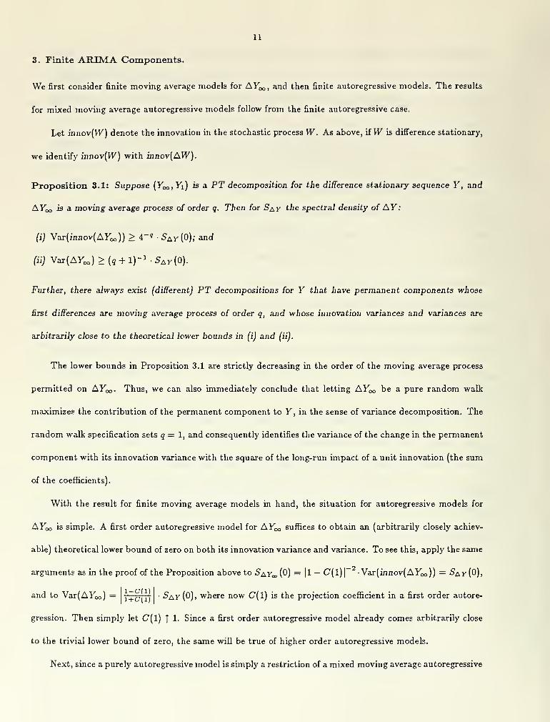
not misled by doing so. Figure 4.1 graphs two diff'erent estimates of the spectral density function for

output growth. One is a smoothed periodogram estimate (using a rectcmgular two-sided filter of length

17), the other is an autoregressive spectral density estimate. For the second, the eight-lag autoregressive

representation is estimated by least squares, then the reciprocal of the square of the fourier transform of the

projection representation is graphed here. Under standard regularity conditions, both of these are pointwise

consistent for the true spectral density function (see for example BriUinger Theorems 5.6.1 and 5.6.2 cind

the surrounding discussion [1981, pp. 147-9] and Berk Theorem 1 [1974]). Notice that the overall shape of

the spectral density estimates in Figure 4.1 are roughly the same, although differing in details.

Our focus here is not the value of the spectral density at any particular fijced frequency, but whether

PT decompositions such as those described in Propositions 2.6 and 3.1 can be found for aggregate output.

Recall that these decompositions are such that the permanent component is smooth in the sense of having

0.00

0.00

Figore 4.1

GNPGrovth

atrtoregressive estimate

0.25 0.50 0.75

V a irvction of PI

1.00

0.00

0.00

Fi^» 4.2

GUP «ad Supply DistarbanoM

0.23 0.50 0.75

Frgqgency as « fraction of PI

— GHPgrovth

— Supply

1.00

0.00

0.00

Figore 4.3

GUP Grovtlt, Hill ItutoTBtiott Varitiwe

0.25 0.50 0.75

Txtfptcucf tB a fraction of PI

— Artaal GUP

— Order 1

- Order 3

Order 5

— Order 10

-- Order 15

1.00

3.00 T

2.50-

Figore 4.4

GNP GrovUc Uia Vuiafioe

0.00

— ActaalGNP

— Order 1

- Orders

Order 5

— Ord«rlD

- Order 13

0.00 0.23 0.30 0.73

Freqaeacy as a fraction of PI

1.00

13

"small" variance.

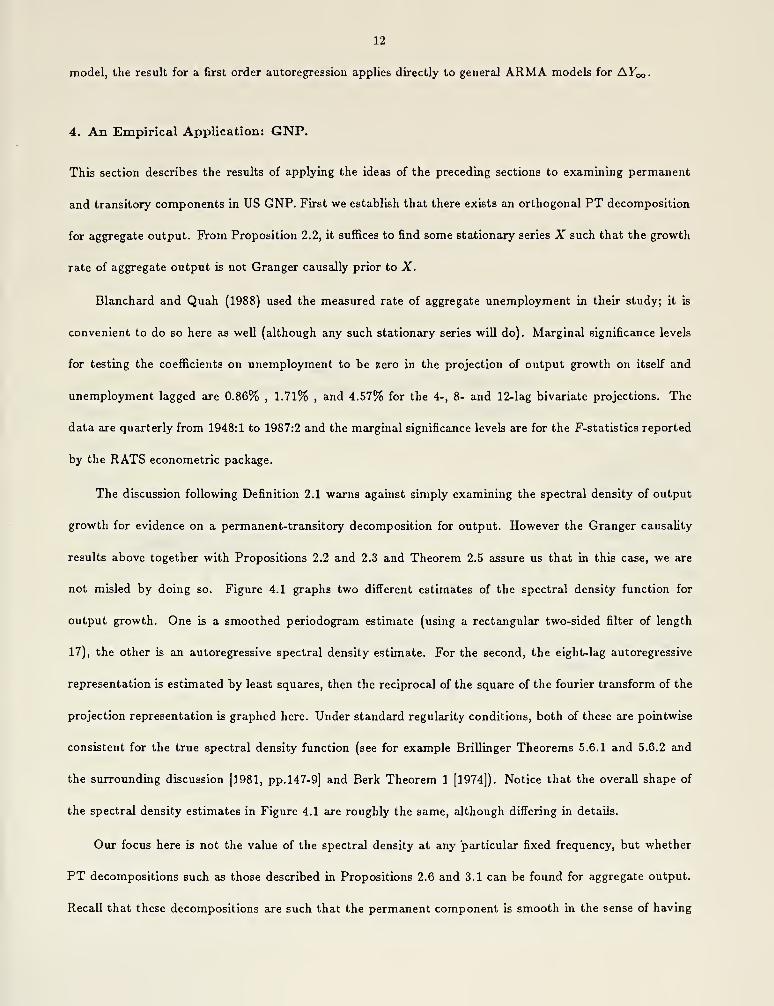
Figure 4.2 presents the estimated spectral densities for the growth in output and in the supply component

of output (in the terminology of Blanchard and Quah). These are smoothed periodogram estimates (unless

specified otherwise, all spectral density estimates hereafter are obtained by smoothing the periodogram

using a rectangular two-sided window of length 17). The supply component is calculated from "historical

realization" by Blanchard and Quah. Due to sampling error, the estimates of the spectral densities at

frequency zero of these two stochastic sequences are not exactly equal: they are 1.83 and 1.76 for the

original data and for the supply component respectively. For the purposes of graphing the spectral densities

in Figure 4.2, that for the supply component is scaled upwards so that the spectral densities coincide at zero.

Notice that even in the presence of sampling error and after upwards scaling, except for one or two ordinates

the estimate for the supply component never exceeds that for the original data. This is an implication of

the orthogonal nature of the supply-demand decomposition in Blanchard and Quah.

The supply component as calculated by those authors is evidently not special in any way, and is certainly

not "trivially implied by their assumptions" (I have heard this assertion made a number of times). The results

that they actually obtain derive precisely from their use of the unemployment rate as the additional indicator

in the system that they estimate. The use of the unemployment rate series is sensible for reasons that are

described in their paper.

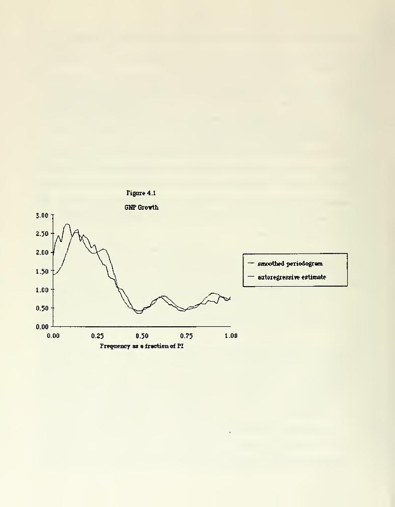
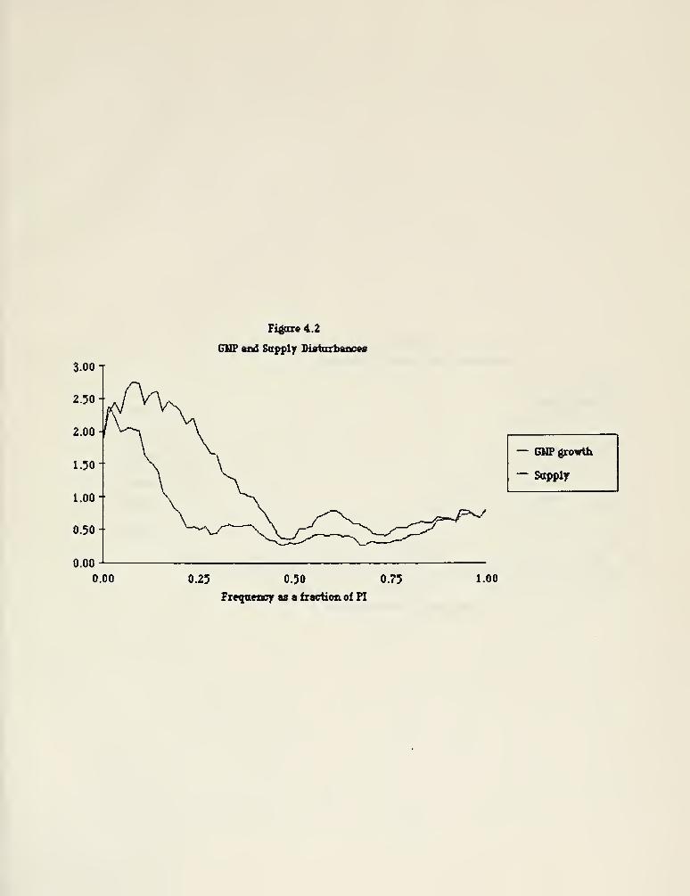
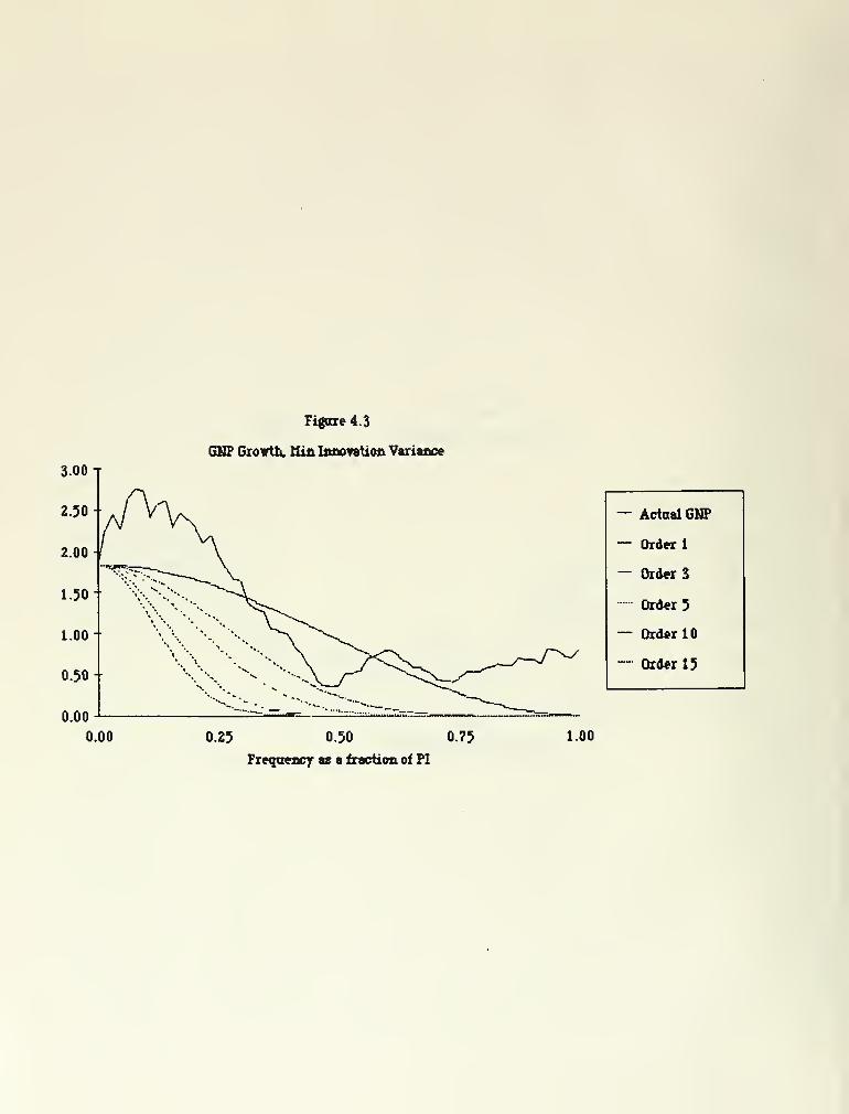
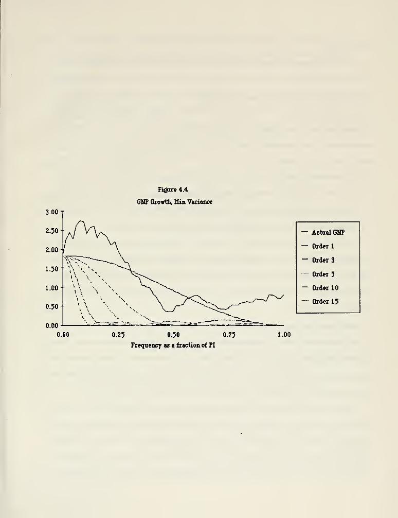
Figures 4.3 and 4.4 again graph the estimated spectral density function for output growth. Superimposed

on this and scaled to coincide at frequency zero are the theoretical spectral densities of moving average

permanent components attaining the lower bounds described in Proposition 3.1. Figure 4.3 graphs the

spectral densities of minimum innovation variance permanent components (part (i) of the Proposition), and

Figure 4.4 graphs those of minimum variance permanent components (part (ii) of the Proposition).

Without explicitly developing precision properties for these estimates, it is difficult to say if an orthogonal

PT decomposition where the permanent component is a pure random walk (say) "fits" aggregate output. The

appropriate condition in these graphs would be that the spectral density at zero must also be the minimum

value for the spectral density everywhere. However we note that if some orthogonal PT decomposition

exists, then there necessarily also exists another such decomposition with a permanent component that is

14

even smoother (in the sense of having a smaller innovation variance or Vtiriance): this follows from the way

in which richer moving average structures collapse in towards the horizontal axis in Figures 4.3 and 4.4.

5. Conclusion.

This paper has considered the general problem of decomposing a difference stationary process into the sum

of a permanent and a transitory component.

It is by now well-known that unit root and trend stationary time series data generate drastically different

implications for classical econometric inference. How does this difference carry over onto the observable

dynamics of economic variables?

We have shown that without lag length restrictions, the permanent component may be arbitrarily

smooth in the sense of having its changes be of arbitrarily small variance. Thus there is a sense in which

the observable dynamics in a unit root sequence is close to that in a trend stationary sequence. The precise

"long run effect" of a disturbance in the permanent component is always identified and identical, regardless

of lag length and orthogonaUty assumptions.

We have also derived exact lower bounds on the variability in the permanent component when that

permanent component is restricted to be a finite ARIMA process. We have shown that the case when

the permanent component is a random walk maximizes the importance of that permanent component for

explaining the observed data.

In application to US aggregate output, the theoretical results here indicate that GNP can be inter-

preted as the sum of a stationeiry component and a permanent component that is arbitrarily smooth. The

supply component that is calculated by Blanchcird and Quah is seen to be one of many possible permanent

components: it is neither the smoothest nor the most volatile.

15

Technical Appendix.

Proof of Proposition 2.2: By the Wold Decomposition Theorem, I „j

iias a unique moving average

representation I I = C * I 1, wiiere C is an array of square-summable sequences, zero except on

the non-negative integers; C(0) is lower triangular; * denotes convolution; and e = (£i,£2)' is serially

uncorrelated with the identity covaxiance matrix, and is fundamental for {AY, X)'. There exists a unique

orthogonal matrix V such that D = CV has its (1,2) entry sum to zero. Writing

(^^\=D*V'e=D*r), where r? =V'e,

we see that r) is fundamental for [AY, X)' , and is serially uncorrelated with variance covariance matrix equal

to the identity. By the construction, such a {D,r]) pair is unique, i.e., no other pair admits simultaneously

a (1,2) entry in the array of moving average coefficients that sums to zero, and a fundamental disturbance

vector that is contemporaneously uncorrelated. Identify AYoo to be Dn * rji, AYi to be D12 * ^2- Since

2,-Ci2{y) = 0, AYi has spectral density that vanishes at frequency zero, so that then Yi itself can be

chosen to be covariance stationary. Suppose then that AY is Granger causally prior to X. This implies that

there exists a moving average representation [AY, X)' = 5 * i/, wiiere the (1,2) entry in B can be taken to

be identically zero; the variance covariance matrix of the serially uncorrelated v is arbitrary. It then follows

that the (1,2) entry in C is identically zero, so that the orthogonal matrix V above is simply the identity.

But then AYi is identically zero so that Var(y"i) = 0. Thus if AV is Granger causally prior to X, a PT

decomposition does not exist. Next suppose the opposite, i.e., consider when AY is not Granger causally

prior to X. Then C12 cannot be identically zero and thus no nontrivial linear combination of Cn and C12

is identically zero. It then follows that both AY^o (or equivalently Dn * rji) and AYi (or D12 * r/sj have

strictly positive variances, and thus are uniquely determined by the above construction. Q.E.D.

Proof of Proposition 2.S: (i) Suppose (1^00,^1) is a PT decomposition for Y. Since Yi is covariance

stationary, S^Yi (w) = at w = 0. By the inequality \S^YiAYa^ \^ S/\Yi • Say„, this implies that at w = 0,

SaYiAY„ = S^YAY„ - S^Y^ = 0. Next, recall that S^Yi = Say^c + ^ay - 2ReS'ArAyco- At w = 0, this

then becomes S^y — SaYoc = 0- Thus we have established (a). Further since VarfAFi) > 0,

Var(Ayi) =J

S^Y.dij =J

[5Ay„(w) + SayH - 2Re5ArAr„(c^)] dw > 0.

16

Next Var(Ayoo) = / S^^y^ (w) > 0, and so we have established (b). To prove the converse, suppose (a). Then

at w = 0, S^Yi = 2S^Y„ — 2Re5'Ar A^co = 2 [5Ay„ — S'Ar^] = 0. Thus Yi can be chosen to be covariance

stationary- By (b), both AYi and AFoo Aave strictly positive variances. Thus (Foo . ^i ) is a PT decomposition

for Y. (a) Suppose (yooi ^'i) ^ an orthogonal PT decomposition for Y. It only remains to establish (c). By

orthogonality, for all w, S^YiAY^ — Sayay„ - Say„ = 0, which implies that Sayay„ = -^Arco- Farther

since for all u, S^n = -^Ay - Say„ > 0, (c.) follows. Conversely, suppose (a) and (b). By (i) (1^00,^1) is a

PT decomposition. In addition, if (c) is true, then AYi is orthogonal to AVoo at all Jeads and iags, so that

(yooi Yi) is an orthogonid decomposition. Q.E.D.

Proof of Corollary 2.4: By Proposition 2.3, (Yoo,Yi) being an orthogonal decomposition for Y implies

that the joint spectral density of (^00,^1)' can be written as S^^y^, (11 / )-^"^ some reai symmetric

positive definite function ip, zero at frequency zero, S^y = (1 + V')^Aroo — ^ay„- But then the projection

of AY on lead, current and lag values of AYoo has coefHcients whose fourier transform is •S'^y^ /•^'aVoo ~ ^^

This is simply the identity however and therefore places zero weight on lead values. Thus AYoo is Granger

causcdly prior to AY. Next the projection of AYoo on lead, current and lag values ofAY has coefficients with

fourier transform {l + if>)~^. When AYoo ^Jid AY do not have exactly the same serial correlation patterns, ip

varies over (— t, +7r]. But then the coefEcient sequence has a fourier transform that is nontrivial and real, and

thus the coefEcient sequence itself is two-sided and symmetric. Consequently AY is not Granger-causally

prior to AYoo- Q.E.D.

Proof of Theorem 2.5: (i) Choose b to be the (one-sided) sequence of Wold moving average coefEcients

for the spectral density S/S^y^, i-^-, \b\^ = •S'^y S- Notice that since S{(jj) = 5'Ay(w) = 5Ay„(w) at

w = 0, we have J^y ^[j] = 1- S'et Xoo = b * Yoo, and Xi = Y — Xoo- The spectral density matrix of the

jointly covariance stationary vector sequence [AXoojAY)' is:

( 5ax„ \^(b 0\( S^Y^ . \ (l' 0\\Sayax„ Say J \0 iJ\Sayay^ S^y J \0 l)

^(\b?SAY^ \^f, S \

Vi5AyAy„ Say„ J Vi-^AyAy^ S^Yo. )'

Thus AXoo has the required dynamics in S. Further since b = 1 atw = 0, and (Yoo, ^i) is a PT decomposition

for Y, this matrix is seen to have all its elements equal at w = 0. Finally, the determinant of this spectral

17

density matrix is

S S^Y - \b\'' \S^Y ^yJ^ = \b\^ det ( Z^'"'--

)X'^AYAYo^ JAY J

which implies:

J \-^AYAX„ ^AY /

Because in addition / S{w) doj > 0, we then have that the variance covariance matrix of (AXoo, Ay)' is full

rank. By Proposition 2.3, (Xoo,-^i) is a PT decomposition for Y. (ii) Since (Foo, Yi) is an orthogonal PT

decomposition for Y , Proposition 2.3 implies that the spectral density matrix of (AVoo , AF )' can be written

as SaYo, I1 1 / )) fo^ V" some positive definite real symmetric function with i>(tL)) = at w = 0. For

b,c square summable sequences, define AXoo{b,c) to be the process b * AFoo + c * Ay. By construction,

(AXqo, Ay)' is jointly covariance stationary, and has spectral density m.atrix given by:

b c\ „ (I I \ f'b'

lj*^^^"l,l 1 + ip) [c' 1

Up to a stochastic process whose first difference vanishes in mean square, Xoo{b,c) is uniquely defined by

the requirement that its first difference be b* AYoo + c * AY. Let Xi(b,c) = Y — X^o (&) c) . By Proposition

2.3, for {Xoo{b,c),Xi[b,c)) to be an orthogonal PT decomposition, it is necessary and sufficient that there

exist symmetric positive definite functions Sx, 4>x, with V'x(w) = at w = 0, such that the spectral density

matrix of (AXqo, Ay) above can be represented as Sx [ .. - , 1 • Set Sx to S in the statement of the

Theorem, and deBne V'x = '^x^^^Ya^i^ + V") — 1 = S~^{Say — S), which is therefore guaranteed to be a

real symmetric positive deSnite function, vanishing at w = 0. Select square summable sequences b,c such

that their fourier transforms b, c satisfy:

— {S/S^Ya,) ' V'x/V' for w ^ 0, and at w = 0;

c=(l + rP)-'[{S/SAYj-b].

Notice that b is restricted only to the extent that its modulus on each frequency satisfies the above equality.

Since the right hand side is real symmetric and positive definite, it is a spectral density. Thus b can be

chosen to be the (one-sided) Wold moving average coefficients corresponding to that spectral density. It is

straightforweird to verify that these sequences b,c imply that:

VO 1 ; U l + rpj\c* l) \Say^J\1 1 + rPxJ

18

Thus {Xoo(b,c),Xi{b,c)) is an orthogona.1 PT decomposition. Q.E.D.

Proof of Proposition 2.6: It is always possible to choose S in the Theorem to be such that ^ J S[(j)da}

is no greater than S. Q.E.D.

Proof of Proposition 3.1: Since AYoo is a moving average process of order q,

AY„ (f) =^ C{j)innov{AY^){t - j), for aU t,

3=0

with C(0) = 1, X^y=o ^(j)^'' 7^ ^ ^"^ Nl ^ 1- Since Yoo is a permanent component for Y,

Var(innov(AF<„)) = Say{0).

Thus the lower bound on Var(innov(Ayoo)) is obtained by solving:

y=o

supc y=o 1 j=0

subject to C(0) = 1, ^ C(j)z' ^ for |2r| < 1.

Recall that any such polynomial Yl'i=o ^(j)^^ above may be written as the product of q monomials:

Z)'=o^(j)^^ = ny=i(l + C'(y)'=^). ^'^^ 1-^0)1 ^ l.y = l. 2,...,g appearing in complex conjugate pairs

if not real. Since \'^C{j)z'\'^ = |n'=i(l + ^U)^)? = n'=i |1 + D{j)z\^, its maximization at z = 1

is equivalent to the maximization of \1 + D(y)p, for each j = 1, 2,...,g. This occurs at D{j) = 1 for

each j. Therefore the solution to the optimization problem attains the value 4'. The lower bound on the

innovation variance is then 4~'• 5Ar(0), and results when the moving average representation for AYoo is

(l + L)''innov{AYoo) , where L is the lag operator. Next, the lower bound on Var(Ayoo) is obtained by

solving:

inf cy^Tcijf(Co-'

3=0

subject to C(0) = 1, E <^0>'' ^ for \z\ < 1, and| J2 C(:?')l^<^^ = Say{0).

3=0 3=0

19

Substituting out for cr^, we need to minimize iYl'i=o ^U)'') I Sv=o ^iJ) subject to the boundary condi-

tions above. First notice that ^^_Q C(y) < (Sy=o I^O)!) • Next apply the Cauchy-Schwarz inequality:

3=0

Therefore we have:

< it\^u)i\\ < l±\cu)A • lE^M = lE^wl •(^+1)-

E^ur]/iy=o 3=0

>(g + i)-^

Notice that C{j) = 1 for j = 0,1, . . . ,q, achieves this lower bound, and because Yl'',=o^^ ~ limATi ^~

i-xl >

this satisfies the boundary conditions as well. Thus Var(Ayoo) > (? + 1)~^S^y{0), and this theoreti-

cal lower bound is evidently approached arbitrarily closely by finite moving average processes of the form

Ey=o A^innov(Ayoo)(f - j), where A < 1. Q.E.D.

20

References

Berk, K.N. (1974): "Consistent Autoregressive Spectral Estimates," Annals of Statistics, 2 no.3, 489-

502.

Beveridge, S. and C.R. Nelson (1981): "A New Approach to Decomposition of Economic Time Series

into Permanent and Transitory Components with Particuliir Attention to Measurement of the 'Business

Cycle'," Journal of Monetary Bkonomics, 7, 151-174.

Blanchard, O.J. and D. Quah (1988): "The Dynamic Effects of Aggregate Demand and Supply Distur-

bances," mimeo, February, MIT.

Brillinger, D. (1981): Time Series, Data Analysis and Theory. San Francisco: Holden-Day.

Campbell, J.Y. and N.G. Mankiw (1987): "Are Output Fluctuations Transitory?" Quarteriy Journal

of Economics , November, 857-880.

Clark, P.K. (1987): "The Cyclical Component in US Economic Activity," Quarterly Journal of Eko-

nomics, November, 797-814.

Clark, P.K. (1988): "Nearly Redundant Parameters and Measure of Persistence in Economic Time

Series," Graduate School of Business, Stanford University, January.

Cochrane, J. (1987): "A Critique of the Application of Unit Roots Tests," University of Chicago Working

Paper, December.

Cochrane, J. (1988): "How Big is the Random Walk Component in GNP?" forthcoming. Journal of

Political Economy.

Diebold, F.X. and G.D. Rudebusch (1988): "Long Memory and Persistence in Aggregate Output," Fi-

nance and Economics Discussion Series, Division of Research and Statistics, Federal Reserve Board, January.

Harvey, A.C. (1985): "Trends and Cycles in Macroeconomic Time Series," Journal of Business and

Economic Statistics, 3 no. 3, 216-227.

Hasbrouck, J. (1988): "Bounding the Variance of the Stationary Component of a Detrended Univariate

Time Series," NYU Department of Finance Working Paper, May.

21

King, R., C. Plosser, J. Stock and M. Watson (1987): "Stochastic Trends and Exonomic Fluctuations,"

NBER Working Paper No. 2229, Cambridge, April.

Nelson, C. (1987): "A Reappraisal of Recent Tests of the Permanent Income Hypothesis," Jonrnal of

Political Economy, 95 No. 3, 641-646.

Nelson, C. and C. Plosser (1982): "Trends and Random Walks in Macroeconomic Time Series," Journal

of Monetary Economics, 10, 139-162.

Rozanov, Y.A. (1965): Stationary Random Processes, San Francisco: Holden-Day.

Shapiro, M. and M. Watson (1988): "Sources of Business Cycle Fluctuations," in Fischer, S. (ed.):

NBER Macroeconomics Annual 1988, Cambridge: MIT Press.

Watson, M.W. (1986): "Univariate Detrending Methods with Stochastic Trends," Journal of Monetary

Economics, July, 18, 1-27.

West, K.D. (1988): "On the Interpretation of Near Random Walk Behavior in GNP," American Eco-

nomic Review, March, 78 no. 1, 202-209.

2 8 10 25

^--Z^

'ji^MI

Ca-^-e'^

Date Due

f^^ou,,^''cf

M/<R 8?991

im.04m 3

m. > s^^^^

m. ^ ^^

Lib-26-67

WITT lIBRARtES OUPL

3 ^DflD DOS 2M3 SMS