The relationship between wealth and health

The relationship

between wealth and

health

Marta Tiainen

University of Helsinki

Faculty of Social Science

Economics

Master’s Thesis

April 2018

1

Tiedekunta/Osasto –

Fakultet/Sektion – Faculty

Faculty of Social Sciences

Laitos – Institution – Department

Economics

Tekijä – Författare – Author

Marta Tiainen

Työn nimi – Arbetets titel – Title

The relationship between wealth and health

Oppiaine – Läroämne – Subject

Economics

Työn laji – Arbetets

art – Level

Master’s Thesis

Aika – Datum – Month

and year

April 2018

Sivumäärä – Sidoantal – Number of pages

44

Tiivistelmä – Referat – Abstract

The thesis is about the relationship between health and wealth. The goal is to show that they are

connected to each other, and that improving health can lead to improve of wealth.

The first part discusses the effect of health on wealth and vice versa. It shows that better wealth

is connected to better health and health increase lead to the wealth increase.

Then there is a theoretical model by Grossman (1972) and which was modified by Jacobson

(2000). The model shows that the health is seen as a stock and that individual can invest into the

health during the lifetime. The model shows also the change, when there is a family without

children (partners can invest into each other’s health) and the family with a child (parents invest

into child’s health). The wage and education effect is shown and developed by Grossman

(1972). The increase in wage leads to increase in health, individual has more money to visit the

doctors. The increase in education also leads to increase in health, but in this case individual

gets more information on healthy lifestyle and follows it.

The literature review shows how education, social status, early childhood, family and nutrition

affect the health. Better educated have better health and higher income. An additional year of

education increases the life. Lower socioeconomic status increases the probability of consuming

unhealthy goods and being less educated. The subjective social status affects the childhood, the

mental health and the income. Family plays a crucial role: the mother’s health, parents

education, family’s socioeconomic status effect the health of a child and the future income. The

low birth weight, mental health problems in childhood and bad nutrition lead to problems in

health in the future and lower income.

When the connection between health and wealth, and factors affecting the health are known, it

is easier to implement policies to increase the total health and wealth. The healthy individual is

more productive and it leads to economic growth, what is another topic and also widely

discussed.

Avainsanat – Nyckelord – Keywords

health, wealth, early childhood, nutrition, education, family, socioeconomic status, subjective

social status, wage

2

Contents

1. Introduction .................................................................................................................................... 3

2. The relation between health and wealth ...................................................................................... 4

2.1 The effect of health on wealth .................................................................................................... 6

2.2 The effect of socioeconomic status on health .......................................................................... 10

3. Theoretical model ......................................................................................................................... 13

3.1. Family effect............................................................................................................................ 17

3.1.1. The husband-wife family .................................................................................................. 17

3.1.2. The parents – child family ................................................................................................ 22

3.2. Wage effect .............................................................................................................................. 26

3.3. The role of human capital ........................................................................................................ 31

4. Literature review .......................................................................................................................... 35

4.1. Education ................................................................................................................................. 35

4.2. Social status and wage ............................................................................................................. 36

4.3. Early childhood, family and nutrition ..................................................................................... 37

5. Conclusions ................................................................................................................................... 38

References. ........................................................................................................................................ 41

3

1. Introduction

There have been many researches founding out that rich people expected to live longer than the

poorer. In 1980 men in the United States who had income in the top 5% of distribution lived 25%

longer than men with the income in the bottom 5%. The recent findings in Britain show the

difference in life expectancy between the top and bottom social classes has increased from five to

nine years (Deaton, 2016). Indeed socioeconomic status, education, wealth, race, place of the

residence and social class are related to mortality and morbidity. Healthier people are better

workers: they work harder and more intelligently. Healthier students have higher cognitive

functioning, what helps them to perform better at the school and give the possibility to get a higher

social status later on.

Most of the public health literature has a strong negative view that the different groups of people are

treated differently within the system and has skeptical view of the value of medical care. McKeown

(1979) concluded that rising living standards, like housing and nutrition, lead to the increasing of

life expectancy. Robert Fogel (1997) also found out that the nutrition is important in the process of

economic development and growth. (Deaton, 2016). So, here I will not discuss the effect of race,

place of the residence and the access to health care; I will focus mostly on health and wealth

relations and the factors like education, family and early childhood.

The relationship between health and wealth is called “gradient”: the health improves when the

income grows, and the poor has worse health than the rich, what means the higher the gradient the

better the health. Poor health decreases the time available for working and decreases the earnings,

at the same time it increases medical expenses, all of these lead to even poorer life than before. I

believe that increasing the health is one way to increase the wealth.

Candeias (2016) studied the effect of diabetes on the economic growth. The number of people

having diabetes is rising. In 2010 around 11.6% of the total health expenditures in the world were

spent on diabetes. Candeias writes: “Diabetes, and other preventable non-communicable diseases,

can lead to increased absenteeism and reduced productivity while at work, inability to work as a

result of disease-related disability, and lost productive capacity due to early mortality and exclusion

from the workplace to take care of sick family members.”

4

Candeias (2016) concludes that preventing diabetes will help to prevent other diseases, like

cardiovascular diseases and cancer, and the households can spend more money on other goods and

services.

In this paper the next section will discuss the relation between wealth and health and how do they

affect each other. Then there is a theoretical model developed by Michael Grossman in 1972 and

modified by Lena Jacobson in 2000. Also Grossman showed how the increase in wage and

education change the health stock. The forth section is based on empirical findings of other

researches that show how early childhood and education affect the health. And for the last are

conclusions.

2. The relation between health and wealth

James P. Smith (1999) made calculations using data from Panel Study of Income Dynamics (PSID).

His researches are based on the data from the United States of America. He made a table (Table 1)

for different age groups and 3 different years (1984, 1989, 1994), where he showed the correlation

between self-reported general health status and income (in 1996 dollars). He noticed that those in

excellent health in 1984 have 74 percent more wealth than respondents in fair or poor health do.

This difference in income is also related to schooling, “median incomes of 1984 college graduates

were $77 000 compared to $ 28 000 among high school dropouts – virtually the same as the income

gradient from excellent to poor health.”(Smith, 1999).

According to Smith, changes in health lead to changes in income. Among those in the age group 35-

44, who reported excellent health in 10 years (from 1984 to 1994) the medium income almost

increased by $100 000, at the same time the income of those who reported fair or poor health

increased only by less than $10 000. So, if the person’s self-estimated health increased from 1984,

his or her income also increased.

The other factors which influence health are risk behaviors – like smoking, eating unhealthy food,

drinking alcohol etc. These risk behaviors are more common in lower socioeconomic groups. For

example, Marmout (1999) has found that the percentage of those with lower incomes or less

education smoking is higher than of those who are well educated or earn more. In 1995, 40 percent

5

of men who had not studied in a high school smoked, while only 14 percent of male college

graduates smoked. Similar health patterns exist for other risk behaviors.

It is also important to mention that periods of poor health in the middle age has a negative impact

on retirement. If the earnings are reduced in the middle age, it will lead to reducing of the pension

and social benefits later on. Smith (1999): “Since health status is positively correlated even across

quite distant ages, a correlation of retirement income and current health may flow from past health

to current retirement income”.

Table 1

Median Wealth by Self-Reported 1984 Health Status

Age Group 1984 1989 1994

All Households

Excellent 68.3 99.3 127.9

Very Good 66.3 81.9 90.9

Good 51.8 59.6 64.9

Poor 39.2 36.0 34.7

25-34

Excellent 28.5 51.5 84.3

Very Good 19.5 34.7 50.1

Good 10.5 17.2 28.2

Fair/Poor 0.9 3.1 10.4

35-44

Excellent 100.1 150.1 194.7

Very Good 81.1 96.3 117.5

Good 49.5 45.3 83.5

Fair/Poor 23.8 15.5 32.4

45-54

Excellent 164.2 198.3 255.8

Very Good 132.1 176.2 186.9

Good 87.8 76.9 97.1

Fair/Poor 59.7 61.6 69.4

Source: Smith JP, Healthy Bodies and Thick Wallets: The Dual Relation between Health and

Economic Status, 1999

6

2.1 The Effect of Health on Wealth

As was mentioned before, health has an important influence on wealth, if the person experience

poor health it may reduce the savings and the current income, at the same time it may increase out-

of pocket savings. Health is a stock, which has potential effects on future income, consumption and

medical expenses.

Smith (1999) made a table (Table 2) using the data from Health and Retirement Survey (HRS) and

from the Asset and Health Dynamics of the Oldest Old Survey (AHEAD). The table consists of two

households, ages 51-61 and ages 70+, and distributions of out-of-pocket medical expenses

separately for those who experienced severe, mild or no new chronic diseases. Smith explained that

severe conditions were defined as cancer, heart condition, stroke, and disease of the lung. All other

onsets defined as mild.

Table 2

Out-of-Pocket Medical Expenditures

Percentiles

HRS (ages 51-61) Between Waves 1-3

(severe new chronic) 32 793 1 985 4 399 11 659 17 108 31 601

(mild new chronic) 49 434 1 072 2 255 6 324 9 489 18 322

(no new chronic) 22 358 868 1 833 4 774 7 983 15 452

severe-with H.I. 159 1 003 2 147 4 407 11 564 16 855 28 233

severe without H.I. 0 143 1 060 4 463 16 503 30 519 64 678

AHEAD (ages 70+) Between Waves

1-2

(severe new chronic) 0 622 1 530 3 150 8 600 16 334 34 188

(mild new chronic) 0 400 980 1 910 5 681 8 894 14 800

(no new chronic) 0 255 800 1 800 4 839 8 000 19 008



7

The results show that the expenses with severe new chronic diseases for average 70+ aged

individual are almost double compare to the one with no new chronic disease. And in the age group

51-61 the difference in expenses is more than double. And in both age groups 2 percent with new

chronic diseases spent more than $30 000.

Smith argues that these results can be helpful to understand savings behavior that “some current

wealth may have been accumulated to deal with today’s health problems”.

The problems in health reduce also the labor supply. In case of family, the spouse can work more

and invest into the partner; this can be seen in section 3. But anyway the current health problems

may reduce the household income in the retirement period.

Another way when health affects savings is when the individuals want to consume more when they

are healthy than during the period when they are sick. So it can be that savings rise if the individual

expect himself to get sick.

Smith (1999) also made an empirical model which estimates effects of new chronic health problems

on household wealth accumulation and the pathways through which savings effects take place. The

data he used was from panel surveys of HRS and AHEAD, he used the ordinary least square

regression models and the results are in table 3. The table has 3 columns (dependent variables),

which shows “between-wave” (there were several surveys conducted in three different years, and

Smith calls these surveys as “waves”) changes in total household wealth, OOP=out-of-pocket

medical expenses and total medical expenses. The results are mean estimates.

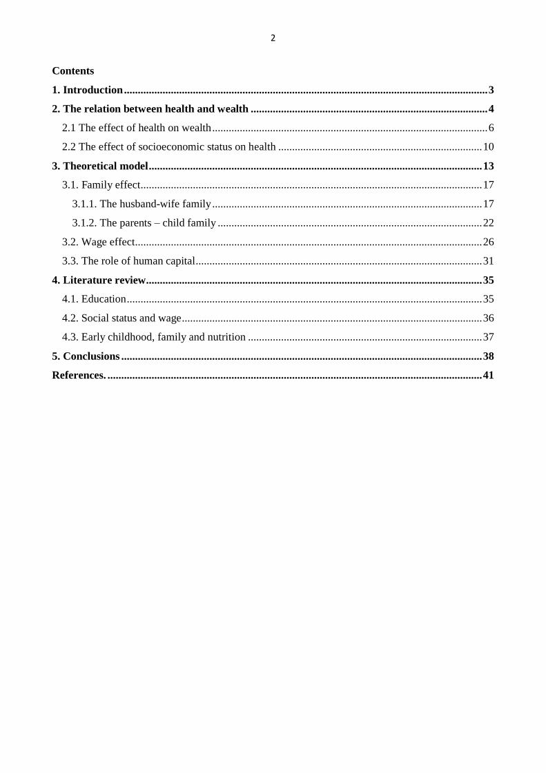
The table 3 shows that even with the mild onset in ages 51-61 with total medical expenditures

$2 555, and the out-of-pocket expenditures are $635, the household wealth is lowered by $3 620.

But with the severe onset diseases, when the out-of-pocket medical expenditures are not yet that

high, the wealth is lowered by $16 846. The change in wealth is even more dramatic for the

household with above median income, the household wealth is lowered by $25 371. There are also

results showing that health insurance doesn’t affect much on the incomes lowering, the difference is

$175.

8

Table 3

Economic Effects of New Health Onset

Wealth OOP Expenses Total Medical Expenses

HRS

Mild onset -3 620 635 2 555

Severe onset -16 846 2 266 28 963

AHEAD

Any onset -10 481 1 026 NA

HRS severe onset only

Below median income -11 348 2 439 29 829

Above median income -25 371 2 014 28 085

AHEAD any onset

Below median income -4 427 915 NA

Above median income -17 040 1 101 NA



Because there was not enough data available for AHEAD, there is no information for mild and

severe onset separated. The table 3 shows that any disease lows the income by $10 481. There is no

information on total medical expenditure in AHEAD, that’s why Smith put NA in the column. In

case of households ages 70+ the income is also has a dramatic lowering for the ones with above

median income - $17 040.

Because table 3 doesn’t show the reasons behind the income lowering, except the health conditions,

Smith made calculations using “empirical models of the alternative pathways though which wealth

accumulation can change – out-of-pocket and total medical expenses, changes in labor supply and

household income, changes in bequest intentions, and changes in mortality expectations. Three

waves of HRS and two waves of AHEAD were used with separate models estimated for changes

observed between each survey wave”. Table 4 shows the results.

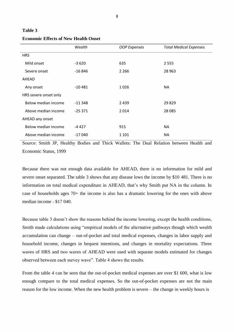
From the table 4 can be seen that the out-of-pocket medical expenses are over $1 600, what is low

enough compare to the total medical expenses. So the out-of-pocket expenses are not the main

reason for the low income. When the new health problem is severe – the change in weekly hours is

9

about 4 hours per week and a 15 percent point decline in the probability of staying at work. And

there is no evidence if the person returns to normal weekly hours. The change in own earnings is

lowered by around $2 600. The table 4 also shows that with new health “shocks” the person also

changes the expectation in probability of living to 75.

Table 4

Pathways of Effects of New Health Events in HRS Survey

(t statistics in parentheses)

Type of

Health Onset

Out-of-Pocket Medical Costs

Total Medical Costs

Change in Probability of

Living to 75

W2-W1 W3-W2 W2-W1 W3-W2 W2-W1 W3-W2

Major 1-2 1 608 (11.3) 792 (3.09) 18 299 (20.0) 11 712 (5.31) -6.59 (5.66) -2.88 (1.96)

Minor 1-2 181 (1.76) 308 (1.68) 230 (0.35) 2 191 (1.38) -1.75 (2.13) -0.207 (0.21)

Major 2-3 NA 1 699 (7.33) NA 23 637 (11.8) NA -5.97 (4.46)

Minor 2-3 NA 677 (3.67) NA 4 534 (2.85) NA -0.91 (0.88)

Type of

Health Onset

Change in Weekly Hours

Probability of Staying at

Work

Change in Own Earnings

W2-W1 W3-W2 W2-W1 W3-W2 W3-W1

Major 1-2 -4.13 (6.09) 0.28 (0.38) -0.15 (7.08) -0.06 (2.24) -2 639 (2.96)

Minor 1-2 -1.45 (2.99) -0.54 (1.04) -0.05 (3.40) -0.02 (1.12) -1 638 (2.57)

Major 2-3 NA -3.92 (6.01) NA -0.16 (7.67) NA

Minor 2-3 NA -1.19 (2.28) NA -0.04 (2.67) NA



At the same time Smith agreed that these results create a puzzle, the out-of-pocket medical

expenditures are not that high compare to the total medical expenditures, and the change in income

own earnings is not that big, but the total change in wealth, shown in table 3, can be dramatic.

Smith explained that it can be caused by “measurement issues that understate medical costs or

household income changes, or that overstate changes in household wealth. Out-of-pocket medical

costs may well understate the full financial costs of an illness. There are expenditures associated

with an illness of a family member – transportation, reconfiguration of home care environments,

and so on – which people may not think of as medical costs and are often not reimbursed. Although

10

household wealth is notoriously difficult to measure, it is not apparent why any errors should be

systematically related to health events unless estimates of wealth shift from optimistic to pessimistic

with the onset of an illness.”

At the same time with the reduction of income, there is possibility for rising consumption of

household; Lillard and Weiss (1993) found out that the marginal utility of consumption increases in

periods of poor health. Also people may “invest” in their siblings or consume at a very high rate.

2.2 The Effect of Wealth on Health

Smith (2005) estimated a probit model using HRS survey data, where he used as variables

education, parental health and education, wealth and health during childhood. The results can be

found in Table 5.

Table 5

Probits predicting the future onset of major and minor chronic diseases

Major condition Minor condition

SES Indicator Estimate Chi square Estimate Chi square

Income 0.0456 0.93 -0.0044 0.00

Wealth -0.0040 1.60 -0.0001 0.00

Change in stock wealth -0.0008 1.06 0.0003 0.75

12-15 years schooling -0.0783 2.66 -0.0527 1.38

College or more -0.0483 0.52 -0.0927 2.33

Health excellent or very

good as child

-0.0870

4.68

0.0042

0.01

Not poor during childhood -0.0949 6.31 0.0155 0.20

Mother’s education 0.0028 0.18 0.0004 0.00

Father’s education -0.0018 0.09 -0.0046 0.72

Father alive -0.1362 1.34 -0.2001 3.32

Age of father at death -0.0001 0.00 -0.0014 0.88

Mother alive -0.0743 0.49 -0.2465 6.51

Age of mother at death -0.0002 0.09 -0.0028 4.60

Source: Smith JP (2005) Unraveling the SES-Health Connection. RAND

11

From the Table 5 can be seen that Smith found that for the major onsets, better health and wealth

reduce the risk of incurring a serious health onset in 50s. For the minor onsets, parental health

reduces the risk of getting new chronic disease in 50s. From the Table 5 it is also seen that the

education plays a crucial role for both major and minor onsets.

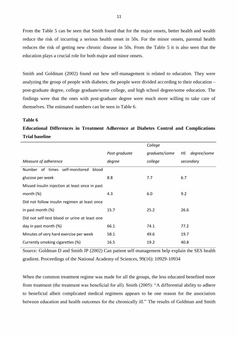
Smith and Goldman (2002) found out how self-management is related to education. They were

analyzing the group of people with diabetes; the people were divided according to their education –

post-graduate degree, college graduate/some college, and high school degree/some education. The

findings were that the ones with post-graduate degree were much more willing to take care of

themselves. The estimated numbers can be seen in Table 6.

Table 6

Educational Differences in Treatment Adherence at Diabetes Control and Complications

Trial baseline

Measure of adherence

Post-graduate

degree

College

graduate/some

college

HS degree/some

secondary

Number of times self-monitored blood

glucose per week

8.8

7.7

6.7

Missed insulin injection at least once in past

month (%)

4.3

6.0

9.2

Did not follow insulin regimen at least once

in past month (%)

15.7

25.2

26.6

Did not self-test blood or urine at least one

day in past month (%)

66.1

74.1

77.2

Minutes of very hard exercise per week 58.1 49.6 19.7

Currently smoking cigarettes (%) 16.5 19.2 40.8

Source: Goldman D and Smith JP (2002) Can patient self-management help explain the SES health

gradient. Proceedings of the National Academy of Sciences, 99(16): 10929-10934

When the common treatment regime was made for all the groups, the less educated benefited more

from treatment (the treatment was beneficial for all). Smith (2005): “A differential ability to adhere

to beneficial albeit complicated medical regimens appears to be one reason for the association

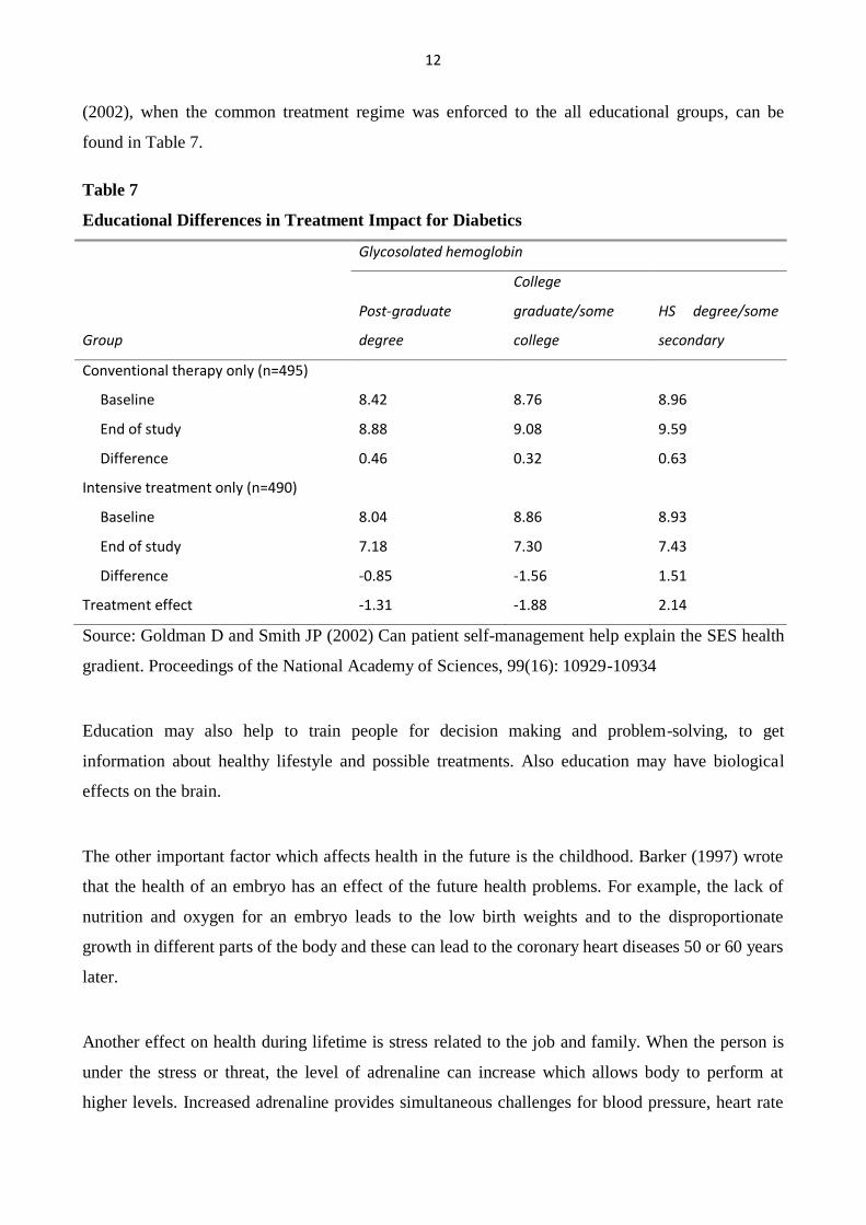
between education and health outcomes for the chronically ill.” The results of Goldman and Smith

12

(2002), when the common treatment regime was enforced to the all educational groups, can be

found in Table 7.

Table 7

Educational Differences in Treatment Impact for Diabetics

Glycosolated hemoglobin

Group

Post-graduate

degree

College

graduate/some

college

HS degree/some

secondary

Conventional therapy only (n=495)

Baseline 8.42 8.76 8.96

End of study 8.88 9.08 9.59

Difference 0.46 0.32 0.63

Intensive treatment only (n=490)

Baseline 8.04 8.86 8.93

End of study 7.18 7.30 7.43

Difference -0.85 -1.56 1.51

Treatment effect -1.31 -1.88 2.14

Source: Goldman D and Smith JP (2002) Can patient self-management help explain the SES health

gradient. Proceedings of the National Academy of Sciences, 99(16): 10929-10934

Education may also help to train people for decision making and problem-solving, to get

information about healthy lifestyle and possible treatments. Also education may have biological

effects on the brain.

The other important factor which affects health in the future is the childhood. Barker (1997) wrote

that the health of an embryo has an effect of the future health problems. For example, the lack of

nutrition and oxygen for an embryo leads to the low birth weights and to the disproportionate

growth in different parts of the body and these can lead to the coronary heart diseases 50 or 60 years

later.

Another effect on health during lifetime is stress related to the job and family. When the person is

under the stress or threat, the level of adrenaline can increase which allows body to perform at

higher levels. Increased adrenaline provides simultaneous challenges for blood pressure, heart rate

13

and the immune system. In the short-run this changes are not dangerous, but when the stress occurs

too often, the results can lead to disease, like high blood pressure, diabetes or cholesterol.

Income inequality is also one of the factors which affect health. A common idea is that the social

inequality raises levels of psycho-social stress which negatively affects adrenaline and

immunological processes. In industrial countries the material level matters less than the fact being

at the bottom in the social ranking. (Smith, 1999).

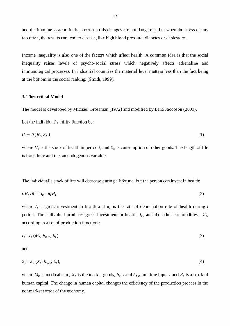
3. Theoretical Model

The model is developed by Michael Grossman (1972) and modified by Lena Jacobson (2000).

Let the individual’s utility function be:

, (1)

where is the stock of health in period t, and is consumption of other goods. The length of life

is fixed here and it is an endogenous variable.

The individual’s stock of life will decrease during a lifetime, but the person can invest in health:

t = - , (2)

where is gross investment in health and is the rate of depreciation rate of health during t

period. The individual produces gross investment in health, , and the other commodities, ,

according to a set of production functions:

= ( , ; ) (3)

and

= ( , ; ), (4)

where is medical care, is the market goods, and are time inputs, and is a stock of

human capital. The change in human capital changes the efficiency of the production process in the

nonmarket sector of the economy.

14

The individual stock of health over time is expressed by:

, (5)

where is transfers and is wealth, and are the prices of and , is the wage rate,

is time in market work and r is the market interest rate.

Health has an effect on market income through the effect on wage and the time in market work.

Jacobson assume that wage rate ( ) depends on health capital ( ) and human capital ( ), so it

can be thought as “labor market earnings rate of return on human capital”.

The total time available is shaped by time spent sick ( , time in market work ( ), time spent

in producing health ( ) and time spent in other commodities ( :

Ω = + + + . (6)

The model assumes that is inversely related to the stock of health, ∂ /∂ <0. If Ω would be

measured in number of days in a year, the would be the number of healthy days:

= Ω - . (7)

Grossman explains that the time which is spent on a visit to a doctor is not a sick time, but the time

invested in health.

The individual can spend his wealth partly on market goods, partly on nonmarket production time,

and part is lost due to sickness. The problem is to maximize lifetime utility by choosing the paths

of the control variables and :

Max. U=

s.t.

= –

Ω = + + +

H(0)= , W(0)= , and given

15

H(T)= , W(T)= ,

T free

and for all tϵ[0,T] (8)

where is individual’s subjective rate of time preference,

and

are the equations of motion

for the state variables, H and W, T is the time of death and t is the present time.

To solve the problem the Hamiltonian is formed:

– ,

From Hamiltonion the interior solution is found and the Langrangian is formed:

– Ω

], (9)

where is the lagrange multiplier for the time restriction, and are costate variables.

is the increase in lifetime utility if health in period t is increase by one unit of health capital. When

the budget is binding is high. According to Jacobson (2000) and can be considered as

measures of economic and time stress.

F.O.C (interior solution):

for all tϵ[0,T]

equation of motion for the state variable H (10)

equation of motion for the state variable W

equation of motion for


From these F.O.C. follow:

(11)

16

since = ( , ; ). Rearranging the equation (11) is found:

. (12)

To make equation (12) simpler it is assumed that what is the effective price of

medical care goods and services ( ):

, (13)

and

. (14)

From equation (13) is seen that when or are high, will be high too, and it means that the

individual’s stock of health is low.

(15)

, (16)

where = ( , ; ).

(17)

(18)

, (19)

where , is marginal utility of health capital, is the marginal

effect of health on wage and is the marginal effect of health on the amount of sick time.

From the rearranging equation (19) can be seen that is depend on the rate of depreciation, the

marginal effect of health on wage and the valuation of time. So, like in equation (14) when the

depreciation rate increases, will increase and the health stock will decrease. When wage

increases the individual will invest more in health and will decrease. And the higher valuation

of time will increase the investments in health, which also leads to decrease of :

.

17

(20)

Since , combining the equation (14) and (19):

. (21)

Putting equation (20) and (13) to equation (21):

(22)

The equation (22) is divided by :

(23)

And now all the parameters are moved to the right side of equation and here is the solution to the

maximization problem:

, (24)

. (25)

Equation (25) means that individual will invest in health until the marginal benefit of new health

equals the marginal cost of health.

Jacobson (2000): “…the solution shows that decreases over time with a rate equal to the rate of

interest r…the individual is free to borrow and lend capital at each period of time…but is

restricted to be non-negative…”

3.1 Family effect

Jacobson (2000) extended Grossman model to show that family also effects on health: the husband

can invest in the wife’s health (and vice versa), the parents can invest in child’s health.

3.1.1Husband-wife model

The extended model includes the variables for husband, m (male), and wife f (female). Basic

assumptions are the same like in the first model. The utility function is:

, (26)

18

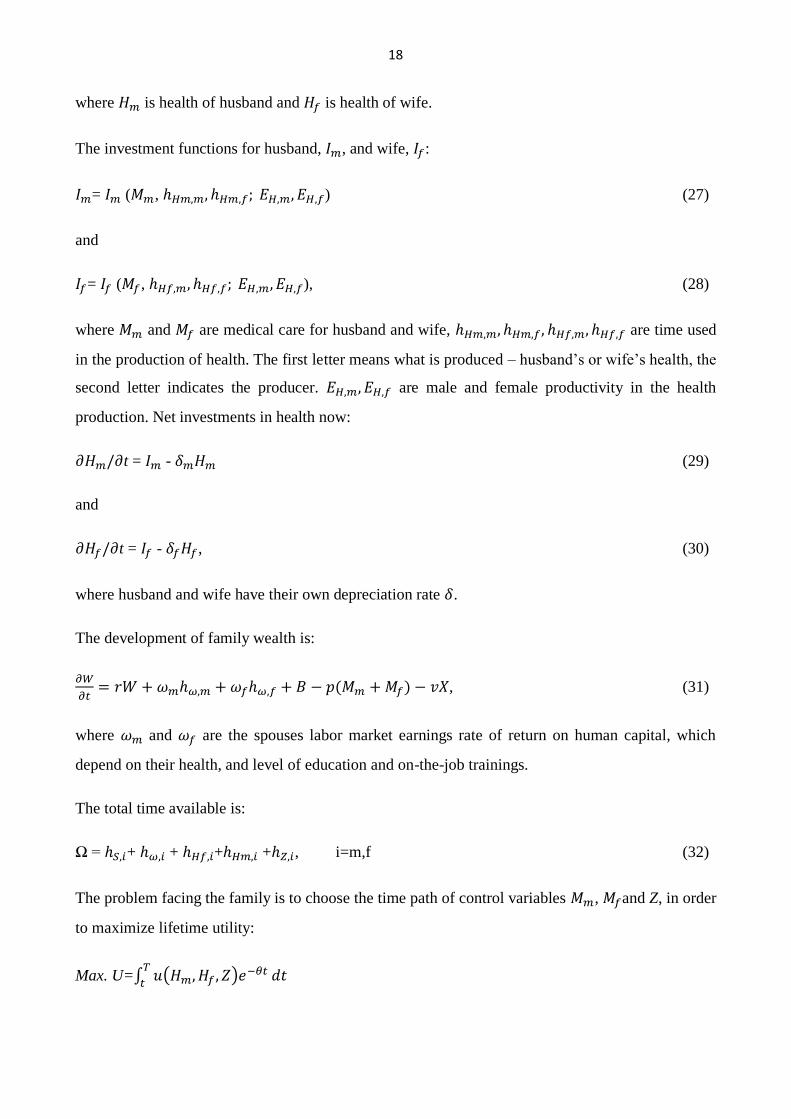
where is health of husband and is health of wife.

The investment functions for husband, , and wife, :

= ( , ) (27)

and

= ( , ), (28)

where and are medical care for husband and wife, are time used

in the production of health. The first letter means what is produced – husband’s or wife’s health, the

second letter indicates the producer. are male and female productivity in the health

production. Net investments in health now:

t = - (29)

and

t = - , (30)

where husband and wife have their own depreciation rate .

The development of family wealth is:

, (31)

where and are the spouses labor market earnings rate of return on human capital, which

depend on their health, and level of education and on-the-job trainings.

The total time available is:

Ω = + + + + , i=m,f (32)

The problem facing the family is to choose the time path of control variables , and Z, in order

to maximize lifetime utility:

Max. U=

19

s.t. t = -

t = -

Ω = + + + + , i=m,f

(0), (0), W(0) given

(T) and/or

W(T) ,

T free

and for all tϵ[0,T]. (33)

T is the lifetime of the husband-wife family, the family “dies” when one of the partners reaches

.


– –

( + ,


– –

Ω ]+ Ω

] (34)


for all tϵ[0,T]

equation of motion for the state variable H for husband (35)

20

equation of motion for the state variable H for wife





To make calculations easier to read m and f are substituted by i (i=m,f) in some equations:

– – = –

From the interior F.O.C. follow:

(36)

From equation (36) is found:

= (37)

Like in previous model there is a substitution of by .

= (38)

, (39)

where = ( ; ).

(40)

(41)

– (42)

(43)

(44)

21

, (45)

The equations (37) and (38) are set in equation (45):

(46)

Equation (43) is set to equation (46) and then divided the whole equation by :

(47)

Then all terms moved to the left, and substituted i by m and f:

(48)

The optimal condition for husband:

(49)

and for wife:

. (50)

In this model the optimal condition, equations (49) and (50), is not valid anymore.

To get the marginal condition equations (49) and (50) are rearranged, the marginal utility of the

health is left on the left side and the rest is put on the right side and the expression (49) for husband

is divided by the expression (50) for wife:

, (51)

the equation (51) is reduced by , and the marginal condition is:

. (52)

22

It means that both partners invest in health until the rate of marginal consumption benefits equals

the rate of marginal net effective cost of health capital. The net effective cost of health capital

equals the user cost of capital less the marginal investment less the marginal investment benefit of

health capital.

The result derived from equation (37) for lifetime utility for health is:

(53)

It means that partners will invest in health until the rate of lifetime utility of health to the effective

rice of health is equal for all family members.

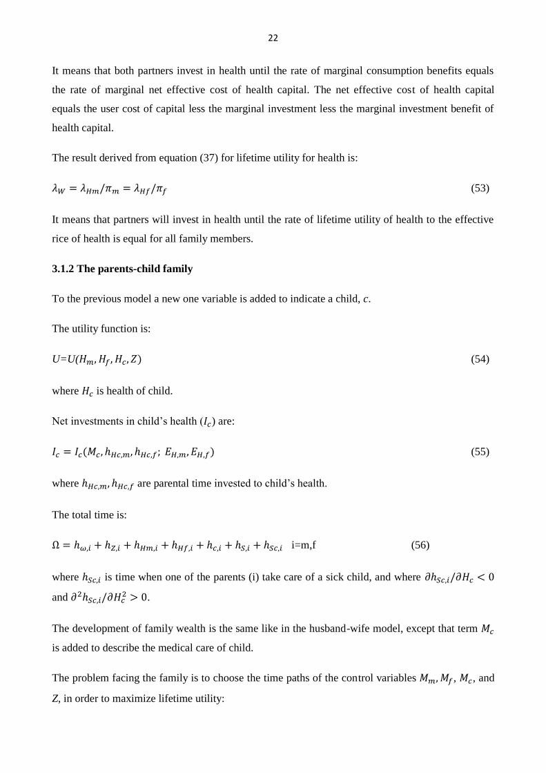
3.1.2 The parents-child family

To the previous model a new one variable is added to indicate a child, c.

The utility function is:

U=U( (54)

where is health of child.

Net investments in child’s health ( ) are:

(55)

where are parental time invested to child’s health.

The total time is:

i=m,f (56)

where is time when one of the parents (i) take care of a sick child, and where

and .

The development of family wealth is the same like in the husband-wife model, except that term

is added to describe the medical care of child.

The problem facing the family is to choose the time paths of the control variables , , and

Z, in order to maximize lifetime utility:

23

Max. U=

s.t. t = - for j=m,f,c

Ω = , i=m,f

(0) for j=m,f,c

for at least one of j=m,f,c

W(T) ,

T free

and for all tϵ[0,T], j=m,f,c. (57)


– – –

,


– – –

, + , + ( + + + [Ω , , , , ,

]+ Ω ]. (58)


for all tϵ[0,T]

equation of motion for the state variable H for husband (59)

equation of motion for the state variable H for wife

24

equation of motion for the state variable H for child






To make calculations easier to read m, f and c are substituted by j (j=m,f,c) in some equations:

– – = – –

From the interior F.O.C. follow:

(60)

From equation (36) is found:

= (61)

Like in previous model there is a substitution of by .

= (62)

, (63)

where = ( ; ).

(64)

(65)

– (66)

(67)

25

(68)

, i=m,f (69)

(70)

Equations (61) and (62) are set to equation (70) and changed j into c:

(71)

Into equation (71) is set equation (67) and the whole equation is divided by :

(72)

All terms are moved to the right, and the solution to the parents-child problem is:

(73)

rewriting the equation (73) gives:

(74)

To get the marginal condition equation (74) is rearranged and the optimal condition is used,

(equation (48) from the husband-wife model, where i=m,f); the marginal utility is left of the health

on the left side and the rest put on the right side and the expression (48) for parents is divided by

expression (74) for child:

,

i=m,f (75)

the equation (75) is reduced by , and the marginal condition is:

. (76)

26

Net effective marginal cost of adult health capital is the same as in equation (52). Net effective

marginal cost of child health is equal to the user cost of child health capital less the marginal

investment benefit of child health, which is the sum of the monetary value of the change in time

taking care of a sick child for father and mother, respectively, for a marginal change in child health.

Equation (53) extends to:

, (77)

implying that the family invests in health until the rate of marginal utilities of (lifetime) health to

effective price of health for all family members is equal and equal to marginal utility of wealth. The

family will not try to equalize the amount of health capital between family members.

Rearranging the equation (77) gives:

, (78)

what means that poor families value a marginal change of child health higher than rich families. In

the family where parents are unhealthy is expected that child health is lower than in “healthy

parents”-family.

3.1 Wage effect

This effect is calculates by Grossman (1972).

It was discussed previously that the wealthier the individual more he can invest into his health. The

less days spent sick mean that the individual can spend more days on market and nonmarket

activities and increase his utility. Thus, the wage rate is positively correlated with the benefits of a

reduction in the time individual loses from the production of money earnings due to sickness and

the benefits from a reduction in time lost from nonmarket production are also positively correlated

with the wage.

Figure 1 shows the shift of demand curve (MEC) when the wage increases from to , where

r+δ is the cost of health capital.

27

Figure 1

Source: Grossman M (1972) On the Concept of Health Capital and the Demand for Health. Journal

of Political Economy, 80(2): 223-255

The figure 1 shows that when the wage increases, the MEC shifts to the right, from to ,

the demand for optimal health stock grows from to , while the cost of health capital stays the

same. The wage elasticity of health capital is:

=(1-K)ε, (79)

where K is the fraction of the total cost of gross investment accounted for by time, and ε is elasticity

of MEC schedule. The wage elasticity is larger, the larger the elasticity of the MEC schedule and

the larger the share of medical care in total gross investment cost.

The increase in wage also has an effect of increasing the demand for medical care. The wage

elasticity of medical care is:

=K +(1-K)ε, (80)

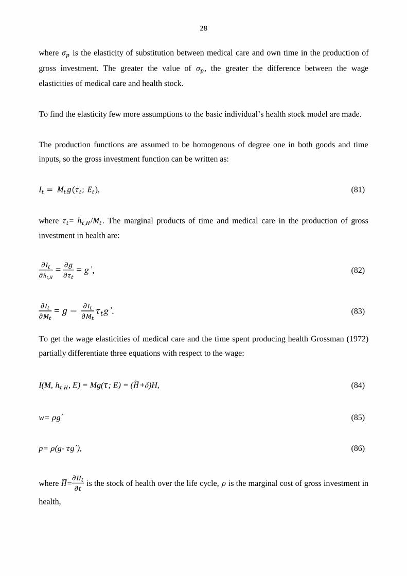
28

where is the elasticity of substitution between medical care and own time in the production of

gross investment. The greater the value of , the greater the difference between the wage

elasticities of medical care and health stock.

To find the elasticity few more assumptions to the basic individual’s health stock model are made.

The production functions are assumed to be homogenous of degree one in both goods and time

inputs, so the gross investment function can be written as:

), (81)

where = / . The marginal products of time and medical care in the production of gross

investment in health are:

=

= g’, (82)

=

g’. (83)

To get the wage elasticities of medical care and the time spent producing health Grossman (1972)

partially differentiate three equations with respect to the wage:

I(M, , E) = Mg( ; E) = ( +δ)H, (84)

w= g´ (85)

p= (g- g´), (86)

where =

is the stock of health over the life cycle, is the marginal cost of gross investment in

health,

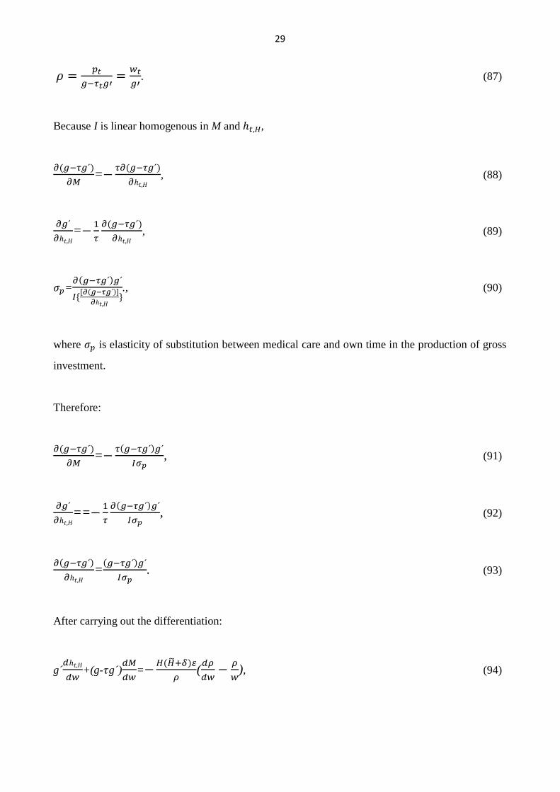
29

. (87)

Because I is linear homogenous in M and ,

=

, (88)

=

, (89)

=

., (90)

where is elasticity of substitution between medical care and own time in the production of gross

investment.

Therefore:

=

, (91)

==

, (92)

=

. (93)

After carrying out the differentiation:

g´

+(g- g´)

=

(

), (94)

30

where is elasticity of the MEC (the shift of demand curve).

1= g´

+ (

+

, (95)

0=(g- g´)

+π[

+

. (96)

With the help of cost-minimization conditions and equation (93) and rearranging terms:

Iε

+w

+p

=

, (97)

I

p

+ p

=I

, (98)

I

+ w

- w

=0. (99)

To solve

in equation (99) Cramer’s rule can be applied):

. (100)

The determinants are:

dM=

(I M+I ε

). (101)

dw=( 2I2)/ M (102)

31

Therefore:

=

( +

). (103)

In elasticity notation, it becomes:

=K +(1-K)ε. (104)

To find the same calculations as previously are done. To solve

in equation (99)

Cramer’s rule can be applied):

. (105)

And it is found:

=(1-K)(ε- (106)

3.2. The Role of Human Capital

This effect is also calculates by Grossman (1972).

The education has an important role for an individual, better educated people are usually earning

more than people without education. Also education changes the productivity in the households and

in the market. Deaton (2016) assumes that better educated people usually have better health; there

are less alcoholic drinkers and smokers. Maybe it caused that people have access to the health

related information and make rational choices.

32

Grossman (1972) proposes that education improves nonmarket productivity. From the basic model

follows that the index of human capital (E) would be:

=M

+

, (107)

where is the marginal product of medical care and is the marginal product of time. The

equation can be rewritten as:

=

=[

](

+(

. (108)

Equation (108) indicates that the percentage change in gross investment supplied to a consumer by

a one-unit change in E is a weighted average of the percentage changes in the marginal products of

M and .

The percentage in the marginal products of medical care and own time for a one-unit change in

human capital:

=

, (109)

= . (110)

If a shift in human capital is “factor neutral”, what means the education has a “neutral” impact on

the marginal products of all factors. :

=

(111)

If education increases productivity, then >0, and equation (108) can be simplified to:

33

= = . (112)

If education increases the marginal products of medical care and own time by certain percent, it

would reduce the price of gross investment by the same percent.

Figure 2 shows the effect of increase in education. It would raise the marginal efficiency of health

capital and shift the MEC schedule to the right, from to , the demand for optimal health

stock grows from to , while the cost of health capital stays the same.

Figure 2

Source: Grossman M (1972) On the Concept of Health Capital and the Demand for Health. Journal

of Political Economy, 80(2): 223-255

The percentage increase in the amount of health demanded for a one-unit increase in E is given by

= ε. (113)

The average cost of gross investment in health is:

34

=(PM+W ) =(P+Wt) . (114)

Given factor neutrality,

. (115)

Therefore,

π=P( , (116)

and

(

´= = . (117)

Taking the total derivative of E in the gross investment function:

=M

M+

+ (118)

Because = and :

. (119)

Because indicates the percentage increase in gross investment supplied by a one-unit increase in

E, shifts in this variable would not alter the demand for medical care or own time if e ualed .

Any effect of a change in E on the demand for medical care or time reflects a positive or negative

difference between and :

M = = (ε-1). (120)

35

Grossman (1972): “E uation (120) suggests that, if the elasticity of the MEC schedule were less

than unity, the more educated would demand more health but less medical care”.

4. Litereture review on the factors increasing the health

There are several researches about the factors influencing health and wealth. Most of them study the

effect of childhood health and education on future income and health. Smith (2007) found that

better health in childhood is related to higher income, higher wealth, more weeks worked and a

higher growth rate of income.

4.1 Education

Strulik (2018) had studied the effect of return to education in terms of wealth and health. Strulik

assumed that every individual had 9 obligatory years of school and studied how the additional year

of schooling would effect on health. He also discussed that the less educated individuals are more

likely to spend money on unhealthy products (such as alcohol and tobacco), than educated. He

concluded that the individuals who care about their health decrease the unhealthy consumption and

increase spending in health. Strulik had done several experiments. One of the experiments shows

the result that the additional year of education changes behavior: the person increases the health

expenditures and decreases the unhealthy consumption. It means that the additional year of

education increases the expectancy of life. He also found that the more educated individuals

demand more health services and benefit more from the medical technological progress.

Oreopolus (2007) studied the effect on health from compulsory schooling. He also found out that

the compulsory schooling increases the life-expectancy. According to his results the year of

compulsory schooling decreases the probability of reporting being in poor health. Compulsory

schooling also lowers the chance of being unemployed and increases the probability of likelihood of

being satisfied with life. He concludes that “lifetime wealth increases by about 15% with an extra

year of compulsory schooling.”

Grossman (2015) had studied the relationship between infant mortality and education. He found that

the schooling coefficient is negative and statistically significant, what helps to “explain” the

decrease in infant mortality and increase in life-expectancy between the years 1910-2000.

36

Grossman discussed different health studies and collected the important results, for example, that

the women in poor countries with more education have less sexual partners and more likely to use

contraception.

4.2 Social Status and Wage

Demakakos et al. (2008) studied the role of subjective social status (SSS). Subjective social status

means where the individual places himself in the social hierarchy. Demakakos et al made an

analysis using cross-sectional data from the second wave (2004-2005) of English Longitudinal

Study of Ageing. The measures were subjective social status, objective social status (which

included education, occupational class and wealth), sociodemographic characteristics (age and

marital status) and health outcome (self-rated health, long-lasting illness or disability, depression,

hypertension, diabetes, central obesity, HDL-cholesterol, triglycerides, fibrinogen, and C-reactive

protein). The results showed that individuals who reported the lower SSS had worse health. Also it

was found that wealth is more related with SSS than occupational class or education. The main

result of this paper is that SSS is related to self-rated health and mental health. Euteneur (2014)

reviewed the works on relation between SSS and health. He also concluded that SSS is related to

self-rated health and mental health.

Karvonen and Rahkonen (2011) studied the relations between SSS and health among the youth.

They collected data at the Finnish schools from 8th

-9th

graders through questionnaires. The

questions included the highest educational level of one of the parents, the occupational status of the

parents, the amount of pocket money the pupil gets, the performance at school, how the pupil put

the family on the social ladder (SSS), self-rated health, long-lasting illnesses and mental health. The

results also showed that the pupils who put their families on the top of social ladder had the better

health. Karvonen and Rahkonen also found that SSS is related with parents’ level of education, with

school performance, with weekly money allowance, and with parents’ employment status.

Komro et al (2016) studied the effect of increasing minimum wage on infant mortality and birth

weight. The research included data from the United States. Komro et al (2016): “We estimated the

effects of state-level minimum wage using a quasiexperimental difference-in-difference research

design.” The result is that one dollar increase in wage decreases the low birth weight births by 1-2%

and decreases the infant postneonatal mortality by 4%.

37

4.3 Early Childhood, Family and Nutrition

All the researches were collected and discussed by Currie (2009).

Currie (2009) studied how parents’ socioeconomic status affects health of child and does health in

childhood affects future educational and market outcomes. Currie showed that wealthier parents are

able to buy more or better quality health inputs, like safer toys, medical care, housing, and

neighborhoods. It is discussed that the difference in health between poor children and rich children

grows with the age. The poor children recover slower and the probability to get a chronic disease is

higher for them, also low SES acts as a stressor and leads to mental health problems. The disease,

like asthma, causes more problems to poor children, because they are less likely to manage properly

their disease. The children from low income families are less likely to be properly diagnosed

because of lack of medical attention. Rich and poor parents have different view on the injuries

which require the medical assistance; it can be seen as one of the reasons of higher rate of children

death in low income families. The risk of obesity is higher for poor children than for rich.

Currie wrote that the poor child health will affect future health, what can affect the labor supply and

productivity. The low socioeconomic status in childhood will affect the health also in the future,

even if the individual gets the higher socioeconomic status. Children from poor families are less

willing to get education what affects their future income. Health in utero is related with birth weight

and metabolism, the unhealthy consumption of mother can lead to brain damage or birth trauma.

Low birth weight babies have lower scores at school and on intellectual and social development

tests; they also have lower probability to be employed as of age 33, same results are as of age 42.

Currie discussed the fetal origins, what means that the exogenous shock caused by conditions

outside the control of mother. One of the examples is famine in the Netherlands during the Second

World War, which is known as “Dutch Hunger Winter”. The babies who were in utero during that

period are more likely to get health impairments, including disorders of central neural system, heart

diseases and antisocial personality disorders. Maternal diseases during the pregnancy have also a

negative influence on babies causing health impairments. It was also found that children who were

infected in utero are less likely to graduate from high school; they are more likely to get low

socioeconomic status due to health disabilities. The same results are in case when mothers drank

38

alcohol being pregnant. The experiments showed that negative shocks to health in utero have

significant effects on the future health and socioeconomic status.

Another effect discussed by Currie is birth weight. It was found that babies who had higher birth

weight are taller and get more schooling. Low birth children are less likely to graduate from high

school. It was found that increasing in birth weight would decrease infant mortality, and for the

higher birth weight the increase in weight will reduce hospital costs. Low birth weight has

significant effect on the future socioeconomic status.

Nutrition plays a crucial role in achieving the higher socioeconomic status in the future. It was

studied in the developing countries, that the children who had better nutrition were more likely to

complete the education and to have higher cognitive abilities. Nutrition in childhood affects the

height, and it is discussed that there is a robust relationship between adult height and earnings.

Mental health problems in childhood strike in the future, the individual loose the income being out

of work place. Children with mental health problems are less likely to finish the high school or to

attend the college. They have lower grades at school and it leads to a lower chance to be employed

in the future. Currie writes: “The available evidence suggests that “externalizing conditions” such as

ADHD (Attention Deficit Hyperactivity Disorder) or aggression have more significant

consequences for outcomes such as completed education and earnings than internalizing

conditions.”

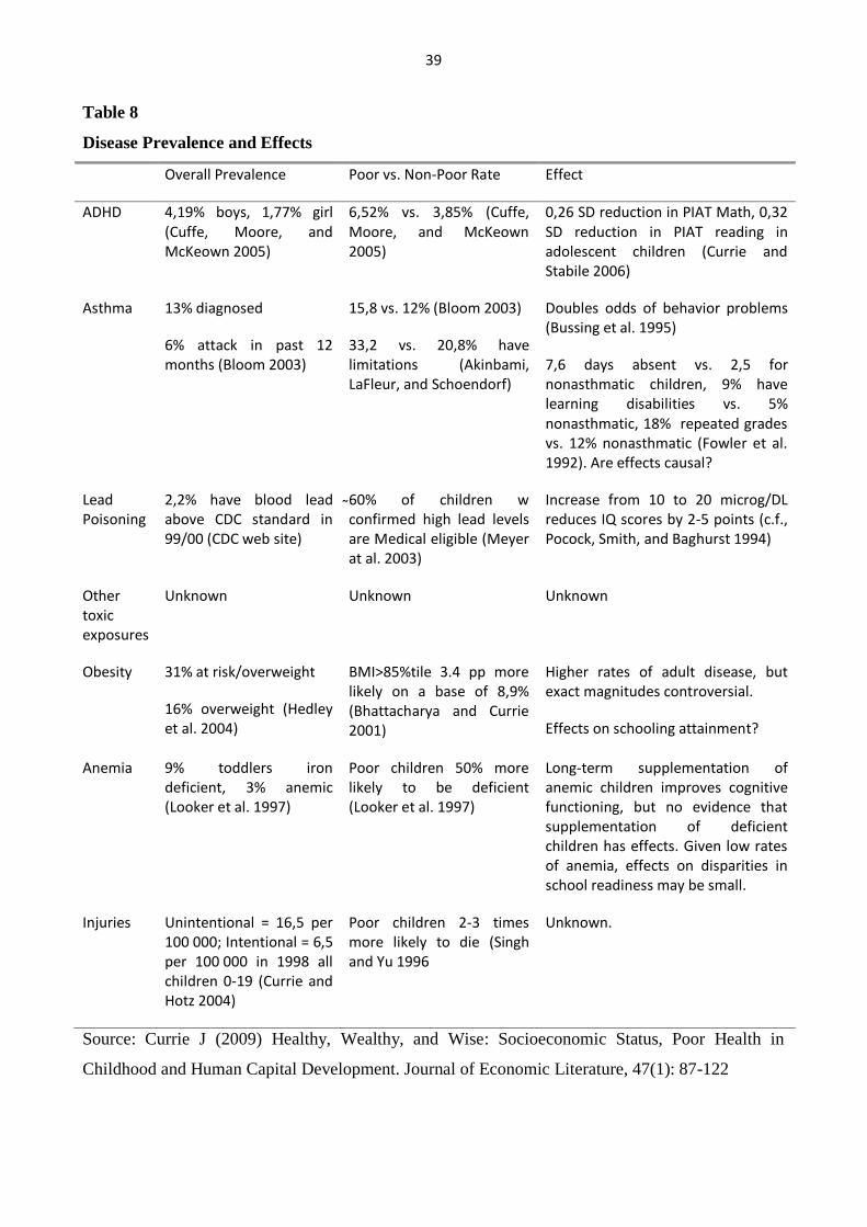
Table 8 copied from Currie (2009) and summarizes the evidence linking several different domains

of child health to outcomes. The researches were made using the data from U.S. CDC stands for

Centers for Disease Control, BMI is for Body Mass Index, PIAT is the Peabody Individual

Achievement Test, and SD is score distribution.

5. Conclusions

In this paper I tried to show the connection between wealth in health. From the previous sections it

can be seen that they are related. It is seen that through health wealth can be increased. When it is

known which factors affect health then it is easier to think about the policies.

39

Table 8

Disease Prevalence and Effects

Overall Prevalence Poor vs. Non-Poor Rate Effect

ADHD 4,19% boys, 1,77% girl (Cuffe, Moore, and McKeown 2005)

6,52% vs. 3,85% (Cuffe, Moore, and McKeown 2005)

0,26 SD reduction in PIAT Math, 0,32 SD reduction in PIAT reading in adolescent children (Currie and Stabile 2006)

Asthma 13% diagnosed

6% attack in past 12 months (Bloom 2003)

15,8 vs. 12% (Bloom 2003)

33,2 vs. 20,8% have limitations (Akinbami, LaFleur, and Schoendorf)

Doubles odds of behavior problems (Bussing et al. 1995)

7,6 days absent vs. 2,5 for nonasthmatic children, 9% have learning disabilities vs. 5% nonasthmatic, 18% repeated grades vs. 12% nonasthmatic (Fowler et al. 1992). Are effects causal?

Lead Poisoning

2,2% have blood lead above CDC standard in 99/00 (CDC web site)

60% of children w confirmed high lead levels are Medical eligible (Meyer at al. 2003)

Increase from 10 to 20 microg/DL reduces IQ scores by 2-5 points (c.f., Pocock, Smith, and Baghurst 1994)

Other toxic exposures

Unknown Unknown Unknown

Obesity 31% at risk/overweight

16% overweight (Hedley et al. 2004)

BMI>85%tile 3.4 pp more likely on a base of 8,9% (Bhattacharya and Currie 2001)

Higher rates of adult disease, but exact magnitudes controversial.

Effects on schooling attainment?

Anemia 9% toddlers iron deficient, 3% anemic (Looker et al. 1997)

Poor children 50% more likely to be deficient (Looker et al. 1997)

Long-term supplementation of anemic children improves cognitive functioning, but no evidence that supplementation of deficient children has effects. Given low rates of anemia, effects on disparities in school readiness may be small.

Injuries Unintentional = 16,5 per 100 000; Intentional = 6,5 per 100 000 in 1998 all children 0-19 (Currie and Hotz 2004)

Poor children 2-3 times more likely to die (Singh and Yu 1996

Unknown.

Source: Currie J (2009) Healthy, Wealthy, and Wise: Socioeconomic Status, Poor Health in

Childhood and Human Capital Development. Journal of Economic Literature, 47(1): 87-122

40

For example, redistribution of wealth is not seen as the best policy, because it is not Pareto efficient.

Redistribution will improve the wealth of low-income group, but reduces the wealth of high-income

group, in total it can be seen that the health of nation stays at the same level, because the loss of

health among the rich will be offset against the gains among the poor.

Grossman model modified by Jacobson shows that health can be viewed as a durable capital stock

where individual can invest in. Partners can invest in to the health of each other, and parents can

invest in health of a child. Jacobson model suggests that there should be different types of families

taken into account when the policies are made.

One of the discussions of this paper is that the fetal health is very important. The improving of

health should include the protection of the health of mothers. The health of child is important not

only for its own sake but it brings a large payoff in terms of future human capital accumulation.

Education is one of the factors that affects both wealth and health, improving the education and

making it accessible for all leads to a better health and wealth conditions. Also new technological

innovations and medical innovations will increase the health. Better access to the medical service

and information would also increase the health.

Improvements in health will not only increase the wealth of an individual, but it leads to economic

growth. There should be more studied which policies could help to improve the unhealthy children

opportunities and how to prevent the affect of past low socioeconomic status on future.

41

References:

Akinbami LJ, LaFleur BJ, and Schoendorf KC (2002) Racial and Income Disparities in Childhood

Asthma in the United States. Ambulatory Pediatrics, 2(5): 382-387

Bhattacharya J, and Currie J (2001): Youths at Nutrition Risk: Malnourished or Misnourished? In

Risky Behavior among Youths: An Economic Analysis, ed. Gruber J, 483-522. Chicago: University

of Chicago Press.

Bloom B, Cohen RA, Vickerie JL and Wondimu EA (2003) Summary Health Statistics for U.S.

Children: National Health Interview Survey, 2001. National Center for Health Statistics: Vital and

Health Statistics, Series 10, no. 216

Bussing R, Halfon N, Benjamin B, and Wells KB (1995) Prevalence of Behavior Problems in US

Children with Asthma. Archives of Pediatrics and Adolescent Medicine, 149(5): 565-572

Candeias V (2016) 5 Reasons why Tackling Diabetes will Boost Economic Growth.

https://www.weforum.org/agenda/2016/04/5-reasons-why-tackling-diabetes-boosts-economic-

growth/

Cuffe SP, Moore Cg., McKeown RE (2005) Prevalence and Correlates of ADHD Symptoms in

National Health Interview Survey. Journal of Attention Disorders, 9(2): 392-401

Currie J and Hotz J (2004) Inequality in Life and Death: What Drives Racial Trends in U.S. Child

Death Rates? In Social Inequality, ed. Neckerman KM, 569-632. New York: Russell Sage

Foundation.

Currie J and Stabile M (2006) Child Mental Health and Human Capital Accumulation: The Case of

ADHD. Journal of Health Economics, 25(6): 1094-1118

Currie J (2009) Healthy, Wealthy, and Wise: Socioeconomic Status, Poor Health in Childhood and

Human Capital Development. Journal of Economic Literature, 47(1): 87-122

Deaton A (2016) Policy Implications of the Gradient of Health and Wealth

Demakakos P, Nazroo J, Breeze E, Marmot M (2008) Socioeconomic Status and Health: The Role

of Subjective Social Status. Social Status & Medicine, 67: 330-340

42

Euteneuer F (2014) Subjective Social Status and Health. Current Opinion in Psychiatry, 27(5): 337-

343

Fogel RW (1997) New Findings on Secular Trends in Nutrition and Mortality: Some Implications

for Population Theory. Handbook of Population and Family Economics 1A

Fowler MG, Davenport MG, Garg R (1992) School Functioning of US Children with Asthma.

Pediatrics, 90(6): 939-944

Goldman D and Smith JP (2002) Can Patient Self-management Help Explain the SES Health

Gradient. Proceedings of the National Academy of Sciences, 99(16): 10929-10934

Grossman M (1972) On the Concept of Health Capital and the Demand for Health. Journal of

Political Economy, 80: 223-255

Grossman M (2015) The Relationship between Health and Schooling: What’s new? Nordic Journal

of Health Economics, 3(1): 7-17

Hedley AA, Ogden CL, JohnsonCL, Carroll MD, Curtin LR, and Flegal KM (2004) Prevalence of

Overweight and Obesity among US Children, Adolescents, and Adults, 1999-2002. Journal of the

American Medical Association, 291(23): 2847-2850

Jacobson L (2000) The Family as Producer of Health – an Extended Grossman Model. Journal of

Health Economics 19: 611-637

Karvonen S and Rahkonen O (2011) Subjective Social Status and Health in Young People.

Sociology of Health & Illness, 33(3): 372-383

Komro KA, Livingston MD, Markowitz S and Wagenaar AC (2016) The Effect of an Increased

Minimum Wage on Infant Mortality and Birth Weight. American Journal of Public Health, 106(8):

1514-1516

Liljas B (1998) The Demand for Health with Uncertainty and Insurance. Journal of Health

Economics 17: 153-170

Lillard L and Weiss Y (1996) Uncertain Health and Survival: Effect of End-of-Life Consumption.

Journal of Business and Economic Statistics, 15(2): 254-268

43

Looker AC, Dallman PR, Carroll MD, Gunter EW, and Johnson CL (1997) Prevalence of Iron

Deficiency in the United States. Journal of the American Medical Association, 277(12): 973-976

Marmot M (1999) Multi-Level Approaches to Understanding Social Determinants. Social

Epidemiology. Berkman L and Ichiro K, eds. Oxford: Oxford University Press

McKeown T (1979) The Role of Medicine: Dream, Mirage, or Nemesis. Princeton, N.J.: Princeton

University Press

Meyer PA, Pivetz T, Dignam TA, Homa DM, Schoonover J, and Brody D (2003) Surveillance for

Elevated Blood Lead Levels among Children – United States, 1997-2001. Morbidity and Mortality

Weekly Report: Surveillance Summaries, 52(10): 1-21

Oreopoulus (2007) Do Dropouts Drop Out Too Soon? Wealth, Health and Happiness from

Compulsory Schooling. Journal of Public Economics, 91: 2213-2229

Pocock SJ, Smith M, and Baghurst P (1994) Environmental Lead and Children’s Intelligence: A

Systematic Review of the Epidemiological Evidence. British Medical Journal, 309(6963): 1189-

1197

Singh GK and Yu SM (1996) US Childhood Mortality, 1950 through 1993: Trends and

Socioeconomic Differentials. American Journal of Public Health, 86(4): 505-512

Smith JP (1999) Healthy Bodies and Thick Wallets: The Dual Relation between Health and

Economic Status. Journal of Economic Perspectives, 13(2): 145-166

Smith JP (2005) Unraveling the SES-Health Connection. RAND

Smith JP (2007) The impact of Socioeconomic Status on Health over the Life-Course. Journal of

Human Resources, 42(4): 739-764

Strulik H (2018) The Return to Education in Terms of Wealth and Health. The Journal of the

Economics of Ageing, 12: 1-14

The relationship between wealth and health

Documents