The Relationship Between the Low Salinity Zone …deltacouncil.ca.gov/sites/default/files/documents/files/10-Outflow... · The Relationship Between the Low Salinity Zone and Delta

Michael L. MacWilliams, Ph.D.

The Relationship Between the Low Salinity Zone and Delta Outflow

Delta Outflows Workshop

February 10, 2014

Outline • Relationship Between X2 and Low Salinity Zone

– Modeling X2 – Low Salinity Zone (LSZ) Modeling

• Relationship Between X2 and Fish Habitat Indices • Estimating Outflow and X2

– Dayflow vs USGS Observations – Surface EC vs Auto-regressive Equations

• Long Term Implications • Conclusions

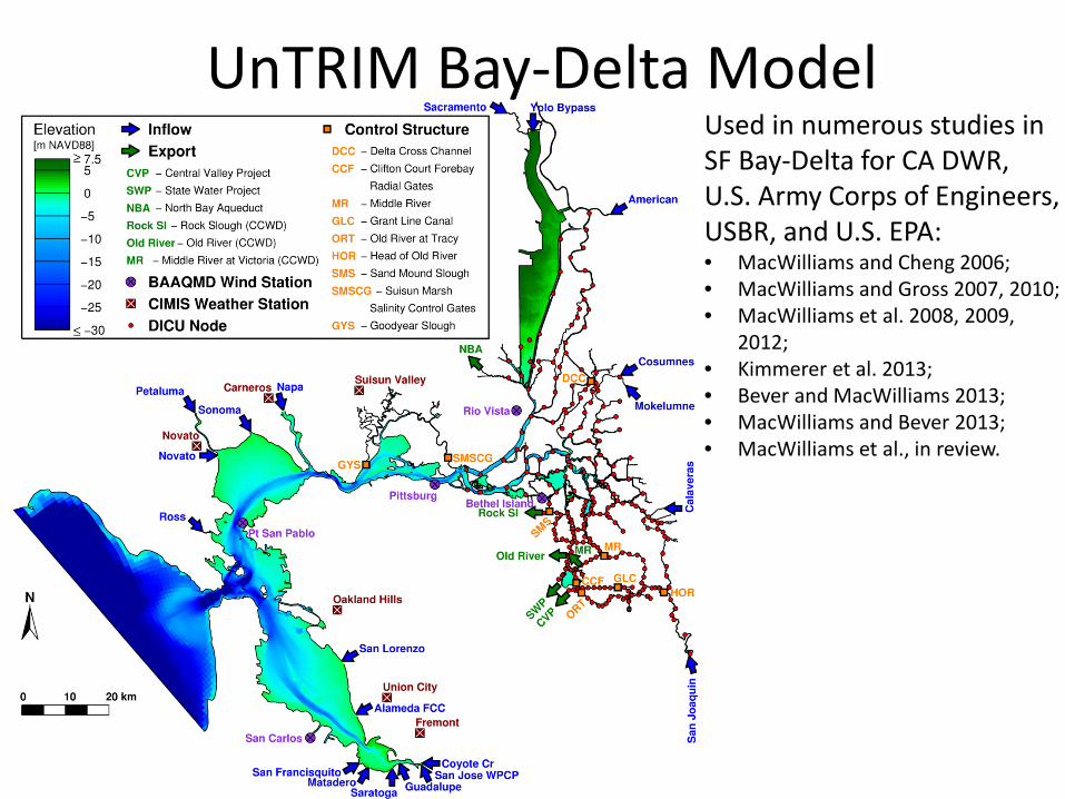
UnTRIM Bay-Delta Model Used in numerous studies in SF Bay-Delta for CA DWR, U.S. Army Corps of Engineers, USBR, and U.S. EPA: • MacWilliams and Cheng 2006; • MacWilliams and Gross 2007, 2010; • MacWilliams et al. 2008, 2009,

2012; • Kimmerer et al. 2013; • Bever and MacWilliams 2013; • MacWilliams and Bever 2013; • MacWilliams et al., in review.

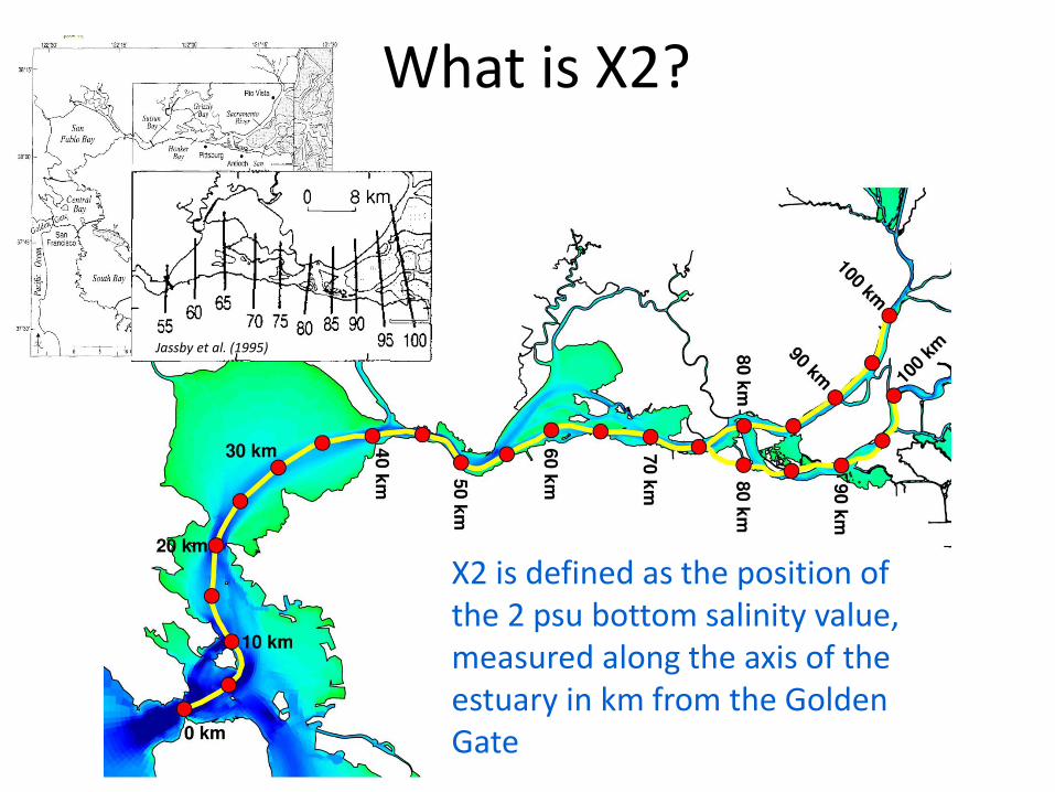
What is X2?

X2 is defined as the position of the 2 psu bottom salinity value, measured along the axis of the estuary in km from the Golden Gate

Jassby et al. (1995)

Low Salinity Zone (LSZ) Area • Calculated from predicted daily-average depth-averaged

salinity in each grid cell. • Total area of region with salinity between 0.5 and 6 psu for

each day.

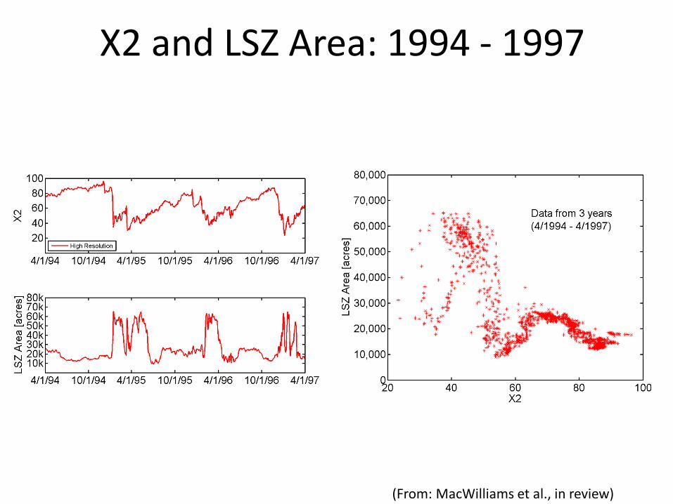
X2 and LSZ Area: 1994 - 1997

(From: MacWilliams et al., in review)

X2 and LSZ Area: 1994 - 1997

(From: MacWilliams et al., in review)

X2 and LSZ Area: 1994 - 1997

(From: MacWilliams et al., in review)

Low Salinity Zone (LSZ): X2 = 75

(From: MacWilliams et al., in review)

Outline • Relationship Between X2 and Low Salinity Zone

– Modeling X2 – Low Salinity Zone (LSZ) Modeling

• Relationship Between X2 and Fish Habitat Indices • Estimating Outflow and X2

– Dayflow vs USGS Observations – Surface EC vs Auto-regressive Equations

• Long Term Implications • Conclusions

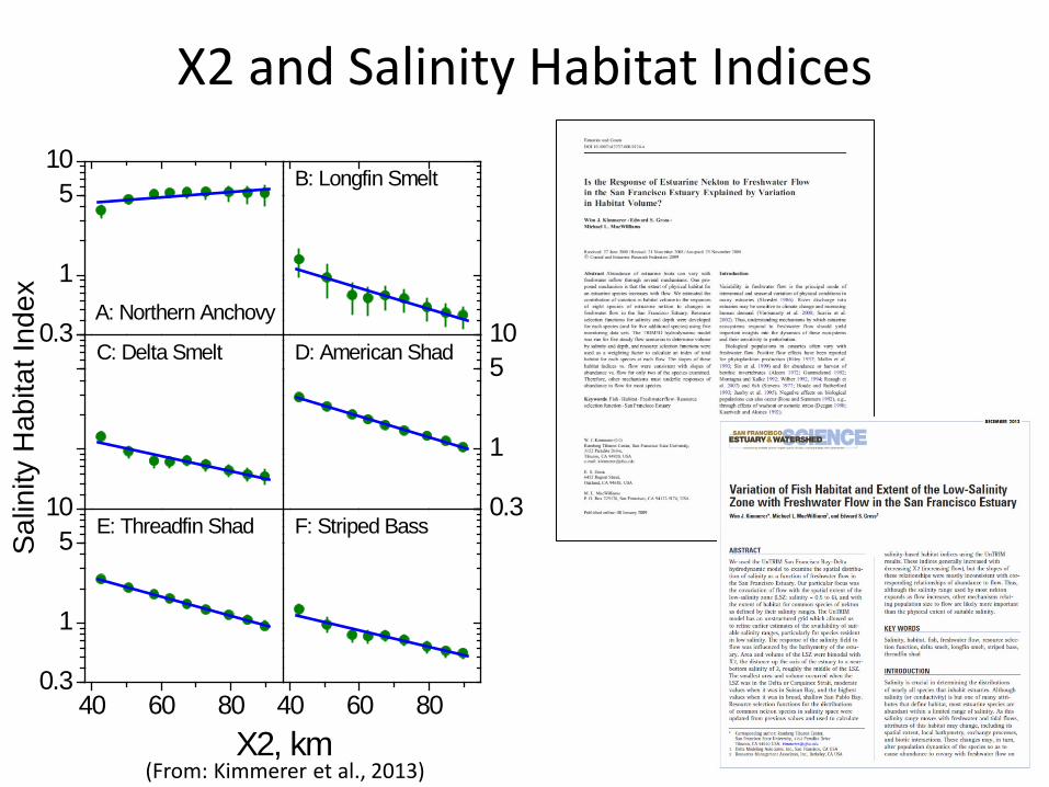
X2 and Salinity Habitat Indices

0.3

1

510

0.3

1

510

40 60 800.3

1

510

40 60 80

A: Northern Anchovy

B: Longfin Smelt

C: Delta Smelt

Habi

tat I

ndex D: American Shad

X2, km

E: Threadfin Shad F: Striped Bass

(From: Kimmerer et al., 2013)

Salin

ity H

abita

t Ind

ex

Outline • Relationship Between X2 and Low Salinity Zone

– Modeling X2 – Low Salinity Zone (LSZ) Modeling

• Relationship Between X2 and Fish Habitat Indices • Estimating Outflow and X2

– Dayflow vs USGS Observations – Surface EC vs Auto-regressive Equations

• Long Term Implications • Conclusions

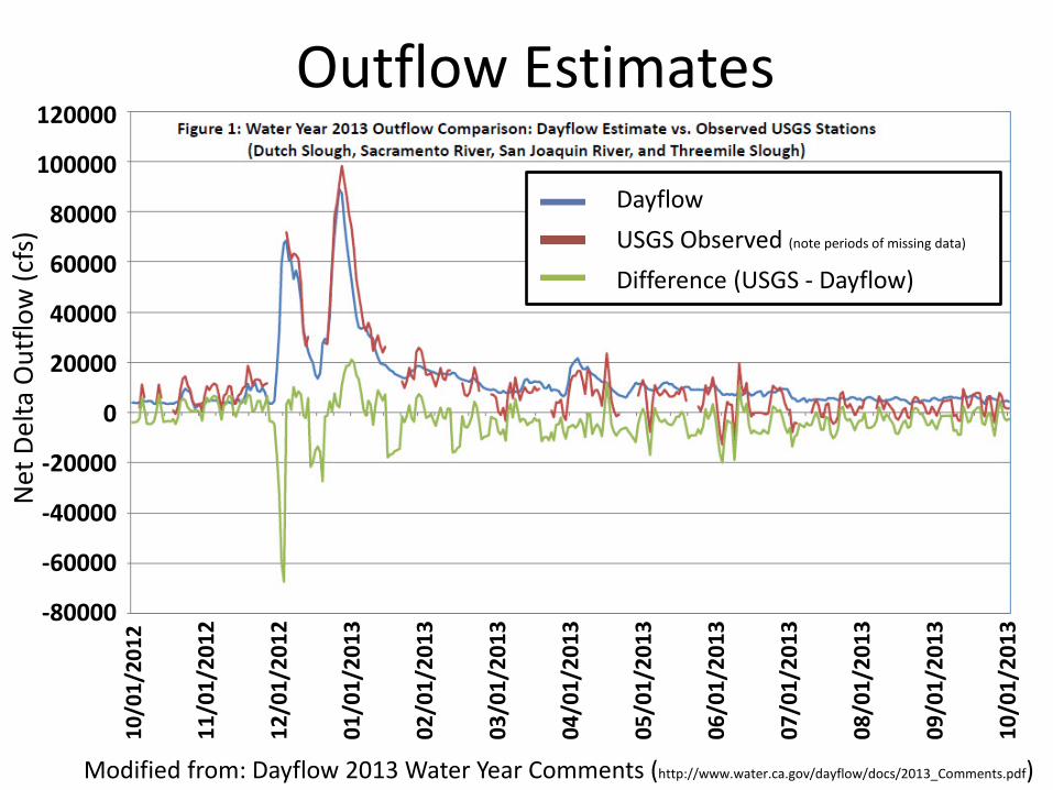
Modified from: Dayflow 2013 Water Year Comments (http://www.water.ca.gov/dayflow/docs/2013_Comments.pdf)

120000

100000

80000

60000

40000

20000

0

-20000

-40000

-60000

-80000

Net

Del

ta O

utflo

w (c

fs)

Dayflow USGS Observed (note periods of missing data)

Difference (USGS - Dayflow)

Outflow Estimates 10

/01/

2012

11/0

1/20

12

12/0

1/20

12

01/0

1/20

13

02/0

1/20

13

03/0

1/20

13

04/0

1/20

13

05/0

1/20

13

06/0

1/20

13

07/0

1/20

13

08/0

1/20

13

09/0

1/20

13

10/0

1/20

13

1) Direct Observations (USGS Cruises) 2) Using Flow-X2 Auto-Regressive Relationships 3) From Observed Surface Salinity (CX2) 4) Using Hydrodynamic Models

How is X2 Estimated?

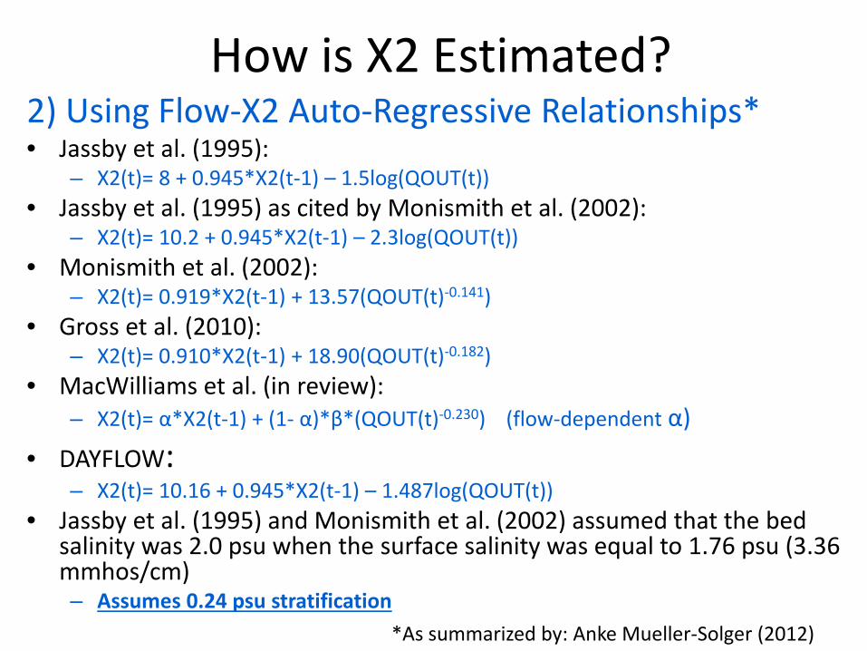
2) Using Flow-X2 Auto-Regressive Relationships* • Jassby et al. (1995):

– X2(t)= 8 + 0.945*X2(t-1) – 1.5log(QOUT(t)) • Jassby et al. (1995) as cited by Monismith et al. (2002):

– X2(t)= 10.2 + 0.945*X2(t-1) – 2.3log(QOUT(t)) • Monismith et al. (2002):

– X2(t)= 0.919*X2(t-1) + 13.57(QOUT(t)-0.141) • Gross et al. (2010):

– X2(t)= 0.910*X2(t-1) + 18.90(QOUT(t)-0.182) • MacWilliams et al. (in review):

– X2(t)= α*X2(t-1) + (1- α)*β*(QOUT(t)-0.230) (flow-dependent α) • DAYFLOW:

– X2(t)= 10.16 + 0.945*X2(t-1) – 1.487log(QOUT(t)) • Jassby et al. (1995) and Monismith et al. (2002) assumed that the bed

salinity was 2.0 psu when the surface salinity was equal to 1.76 psu (3.36 mmhos/cm) – Assumes 0.24 psu stratification

How is X2 Estimated?

*As summarized by: Anke Mueller-Solger (2012)

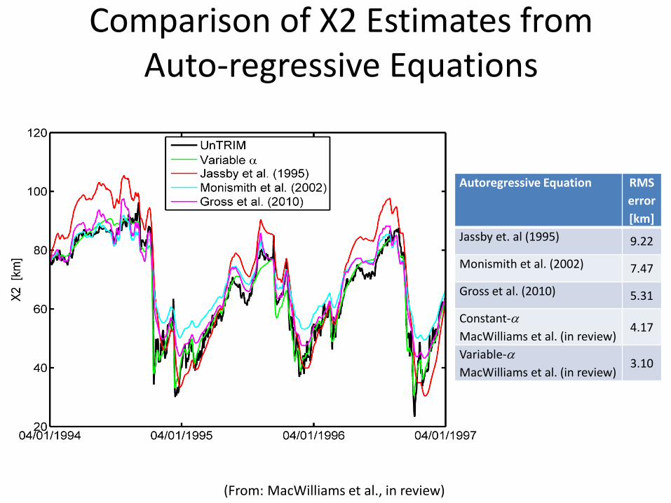
Comparison of X2 Estimates from Auto-regressive Equations

(From: MacWilliams et al., in review)

Autoregressive Equation RMS error [km]

Jassby et. al (1995) 9.22

Monismith et al. (2002) 7.47

Gross et al. (2010) 5.31

Constant-α MacWilliams et al. (in review)

4.17

Variable-α MacWilliams et al. (in review)

3.10

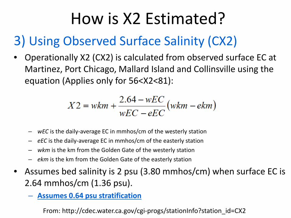
3) Using Observed Surface Salinity (CX2) • Operationally X2 (CX2) is calculated from observed surface EC at

Martinez, Port Chicago, Mallard Island and Collinsville using the equation (Applies only for 56<X2<81): – wEC is the daily-average EC in mmhos/cm of the westerly station – eEC is the daily-average EC in mmhos/cm of the easterly station – wkm is the km from the Golden Gate of the westerly station – ekm is the km from the Golden Gate of the easterly station

• Assumes bed salinity is 2 psu (3.80 mmhos/cm) when surface EC is 2.64 mmhos/cm (1.36 psu). – Assumes 0.64 psu stratification

How is X2 Estimated?

From: http://cdec.water.ca.gov/cgi-progs/stationInfo?station_id=CX2

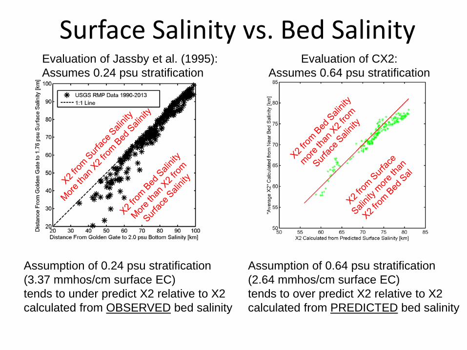
Surface Salinity vs. Bed Salinity Evaluation of CX2:

Assumes 0.64 psu stratification

Assumption of 0.64 psu stratification (2.64 mmhos/cm surface EC) tends to over predict X2 relative to X2 calculated from PREDICTED bed salinity

Assumption of 0.24 psu stratification (3.37 mmhos/cm surface EC) tends to under predict X2 relative to X2 calculated from OBSERVED bed salinity

Evaluation of Jassby et al. (1995): Assumes 0.24 psu stratification

Outline • Relationship Between X2 and Low Salinity Zone

– Modeling X2 – Low Salinity Zone (LSZ) Modeling

• Relationship Between X2 and Fish Habitat Indices • Estimating Outflow and X2

– Dayflow vs USGS Observations – Surface EC vs Auto-regressive Equations

• Long Term Implications • Conclusions

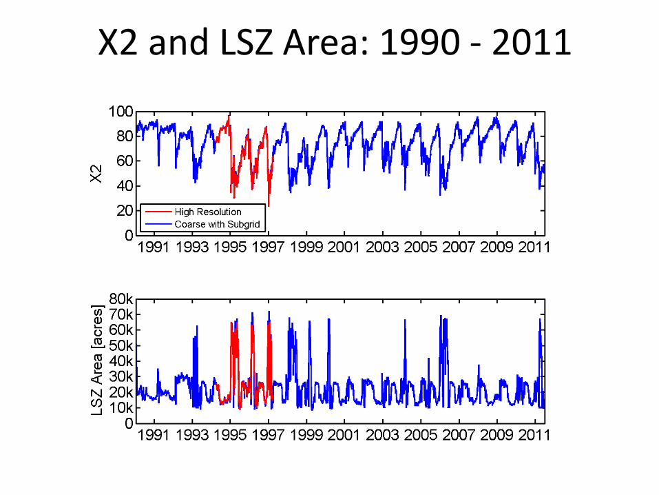
X2 and LSZ Area: 1990 - 2011

LSZ Area vs. X2

Fall LSZ Area: 1990-2010

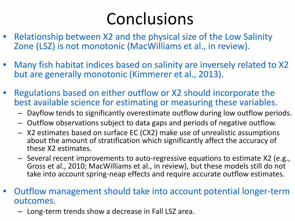
Conclusions • Relationship between X2 and the physical size of the Low Salinity

Zone (LSZ) is not monotonic (MacWilliams et al., in review).

• Many fish habitat indices based on salinity are inversely related to X2 but are generally monotonic (Kimmerer et al., 2013).

• Regulations based on either outflow or X2 should incorporate the best available science for estimating or measuring these variables. – Dayflow tends to significantly overestimate outflow during low outflow periods. – Outflow observations subject to data gaps and periods of negative outflow. – X2 estimates based on surface EC (CX2) make use of unrealistic assumptions

about the amount of stratification which significantly affect the accuracy of these X2 estimates.

– Several recent improvements to auto-regressive equations to estimate X2 (e.g., Gross et al., 2010; MacWilliams et al., in review), but these models still do not take into account spring-neap effects and require accurate outflow estimates.

• Outflow management should take into account potential longer-term outcomes. – Long-term trends show a decrease in Fall LSZ area.

Acknowledgments UnTRIM Model:

Vincenzo Casulli

JANET Grid Generator:

Christoph Lippert

LSZ Expertise:

Bruce Herbold (EPA)

Wim Kimmerer (SFSU)

Edward Gross (RMA)

Larry Smith (USGS)

Fred Feyrer (USBR)

Project Funding:

USACE

CA DWR

USBR

IEP/POD Contact info: [email protected]