The Relationship Between Keynesian Militarism and Economic Growth

1/25

Assist Prof.Dr.Mehmet Mercan

Assoc.Prof.Dr.Özlem Arzu Azer

2/25

Contents

1. The Concept of Military Keynesianism

2. A View to the Military Spending

Worldwide

3. Emprical Analysis

4. Conclusion

1 2

3/25

Popularity of Keynesian

Economics • After Great Depression in 1929, Keynesian

economics took place into the classical

economics since it had seen the negative effect

of non-intervention politics of government.

Keynes emphasized the importance of

consumption and government’s significant role

to increase aggregate demand. Economic

recovery was realized thanks to the New Deal

Program by Roosevelt and II.World War

1 3

4/25

Classical school lost its validity in the process that resulted

in all asset loss of the investors who could not guaranteed

their gaps and the bankruptcy of mediating financial

institutions with the decline of the prices on the Wall Street

and it was estimated that the deficit would be much lower

than expected through the goverment intervention to the

markets on time. A worldwide production losses and

unemployment increases were observed in this great crisis

spreading to the world from the USA.

1 4

5/25

Solving the decline in production and

increasing unemployment problems

happening in the Great Depression in 1929

recognized with the beginning of 2nd World

War beyond the implementation of “New

Deal” programme. Cooperation between

industry, military and politicians realized as a

result of depression and following 2nd

World War

1 5

6/25

The Concept of Military

Keynesianism‘New Deal’ programme carried out for dealing with the

troubles after the Great Deppression and stimulating the

production was not sufficient and resurge of the American

economy accounted for the period after 2nd World War.

Keynesian policies foreseeing an increase in effective

demand with the public expenditures moved to a new

phase with the start of the war and economy was

stimulated through the public expenditures as ‘defence

expenditures’ mainly. 1 6

7/25

The policy of increasing production and

correspondingly effective demand through

the increase in ‘defence expenditures’ called

as ‘Military Keynasianism’ led Keynasian

economy to get heavy criticism.

Some economists argued about the

negative effect of Military Keynesianism in

terms of crowding-out effect and income

redistribution

1 7

8/25

A View to the Military Spending

Worldwide

According to SIPRI data, total military spending in the

World decreased to USD 1.747 billion in 2013 since US

military spending declined by 7.8 % as of USD 640 billion

due to its decreasing role in the overseas military

operations. However, US has still been the toppest country

in the military spending ranking. The top 15 countries’

military spending constitute % 80,5 of total military

spending.

1 8

9/25

Economic Growth as a Driver: Countries to be a

global player, have to complete their power

triangle between economy, politics and military.

Economic growth has been a driving factor to

increase military spending. It is also seen that the

top countries’ military spending ratio to GDP

changes in the range of 1,0 % - 9,3 %. The biggest

military spender countries’ total spending is 77,5 %

of the world military expenditures.

As seen in the table, biggest economies also

spend biggest shares of military spending.

9

10/25

R

a

n

ki

n

g

Country Military Spending (bio,

USD)

Share of domestic GDP,

%

Share of World GDP, %

1 USA 640 3,8 37

2 China 188 2 11

3 Russia 87,8 4,1 5

4 Saudi Arabia 67 9,3 3,8

5 France 61,2 2,2 3,5

6 UK 57,9 2,3 3,3

7 Germany 48,8 1,4 2,8

8 Japan 48,6 1 2,8

9 India 47,4 2,5 2,7

1

0

South Korea 33,9 2,8 1,9

11 Italy 32,7 1,6 1,9

1

2

Brazil 33,5 1,4 1,81 10

11/25

Emprical Analysis

Data Set and Model: In this study, the annual data

of 1988 and 2013 period belonging to the biggest

10 countries (USA, China, Japan, Germany,

France, UK, Brasil, Russian Federation, Italy,

India) worlwide as economic size were used when

the year of 2013 is based on. Variables in the

analysis; real economic growth( growth, with 2005

fixed prices) and military expenditures (milexp, as

a rate for GDP). Data were obtained from World

Development Indicator (WDI).

11

12/25

Coeeficients

Range 1988-2013

growth Economic Growth

milexp military expenditures (as a rate for GDP).

Estimated model in the study is:

13/25

Panel Data Analysis Method

Unit root tests which were used in Panel unit root

tests are classified into two as homogeneous and

heterogeneous models according to the selected data

set. Levin, Lin and Chu (2002), Breitung (2000) and

Hadri (2000) are based on homogeneous model

hypothesis, whereas Im, Pesaran and Shin (2003),

Maddala and Wu (1999), Choi (2001) are based on

heterogeneous model hypothesis.

Since the countries included in analysis are not

homogeneous, Im,Peseran and Shin (2003) (IPS) test

and also different tests will be used in order to

support this test in this study.

14/25

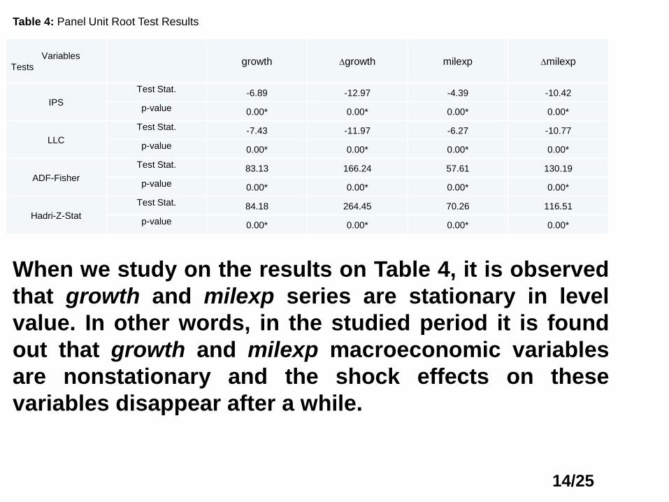
When we study on the results on Table 4, it is observed

that growth and milexp series are stationary in level

value. In other words, in the studied period it is found

out that growth and milexp macroeconomic variables

are nonstationary and the shock effects on these

variables disappear after a while.

Variables

Testsgrowth ∆growth milexp ∆milexp

IPS

Test Stat. -6.89 -12.97 -4.39 -10.42

p-value 0.00* 0.00* 0.00* 0.00*

LLC

Test Stat. -7.43 -11.97 -6.27 -10.77

p-value 0.00* 0.00* 0.00* 0.00*

ADF-Fisher

Test Stat. 83.13 166.24 57.61 130.19

p-value 0.00* 0.00* 0.00* 0.00*

Hadri-Z-Stat

Test Stat. 84.18 264.45 70.26 116.51

p-value 0.00* 0.00* 0.00* 0.00*

Table 4: Panel Unit Root Test Results

15/25

Testing Individual and Time Effects in Fixed

Effects Model (F test) In this stage of the analysis F test was conducted to identify the

existence of individual effects and time effects. Since the selected

countries are energy exporting countries in a certain economic

group, it is forseen that individual and time effects could be

stationary. Whether there are individual and time effects or not can

be decided by F test (Baltagi.2005:34).

With the help of different hypothesis for F test, the existence of

individual and time effects can be tested seperately or together. F

test can be implemented in three different cases as F1, F2 and F3. F1

tests the existence of individual and time effects, F2 tests the

existence of individual effects and F3 tests the existence of time

effects.

16/25

TestStatisctics

Valus

Probability

ValusDecision

F1 29.68 0.00 Individual and Time Effects

F2 3.66 0.00 Individual Effects

F3 10.56 0.00 Time Effects

Table 5: F Tests

When we look at the results on Table 5 in general, we can see that there

are individual effects and time effects. So it is estimated with two-way fixed

effect model.

17/25

Variable Coefficient Stnd. Error t-Statistics Probability Value

growth(-1) 0.555 0.055 10.06 0.000

Milexp -0.209 0.101 -2.067 0.039

constant term 1.793 0.360 4.975 0.000

Diagnostic Tests

R-square 0.74 Avarage dependent variable 2.97

Corrected R-square 0.70 Dependent variable error 4.03

Standard error for equation 2.20 Akaike info criterion 4.55

Square error sum 1042.82 Schwarz criterion 5.06

Log likelihood -533.26 Hannan-Quinn criterion 4.75

F statistics 17.64 (0.00) Durbin Watson statistics 2.30

Jarque-Bera 417.35 (0.00)

Lagrange Multiplier (LM) Heteroscedasticity Test Probability Value: 0.326

Decision: (H0 ret), No heteroscedasticity problem.

Breusch Pagan Autocorrelation Test Probability Value: 0.157

Decision: (H0 ret), No autocorrelation problem.

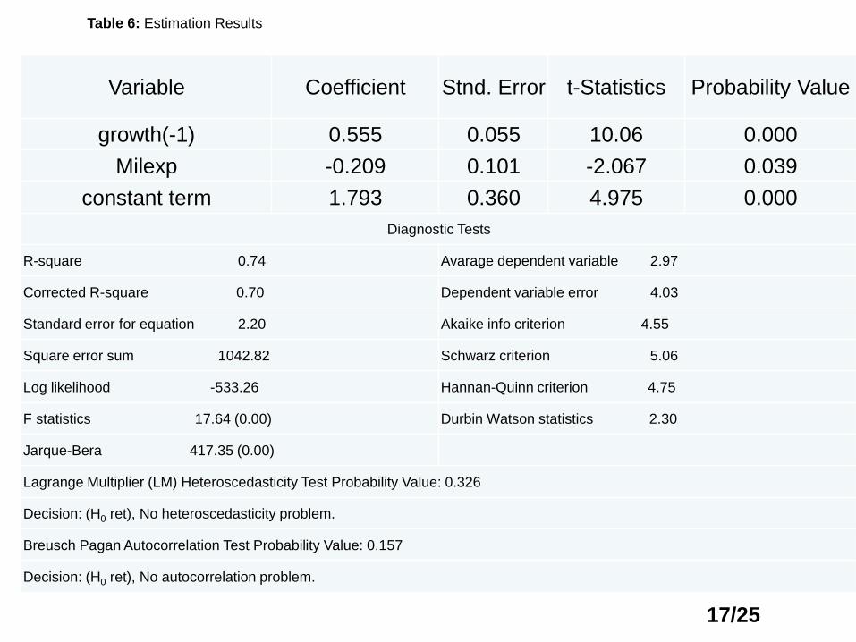
Table 6: Estimation Results

18/25

When we look to the diagnostic test statistics on

Table 6, we can see that model is statistically

reliable. Also it is observed that there is no

heteroskedasticity problem in the model and

autocorrelation problem is solved by adding a

lagged one of dependent variable to the model.

Estimation results are reliable and interpretable.

19/25

When the analysis results are studied on Table 6,

it is identified that increases in military

expenditures in searched countries affected

economic growth negatively and the hypothesis

in question (Benoit Hypothesis) was valid. 10 %

of increase in military expenditures declines

economic growth 2.09 %.

20/25

Conclusion • Effects of military expenditures on economic growth

were discussed by economists and counter-views were

profounded.

• In terms of positive effects of military expenditures on

economic growth, while it is emphasized that they

especially cause technological developments and their

increasing effect on aggregate demand by providing

employment, in critical approaches their exclusionary

effects of private sector as a result that government

shifted their resources to military expenditures are

featured and by a group of economists it is pointed out

that military expenditures are unproductive.

1 20

21/25

• In our study the biggest 10 economy in the world were

handled with the data between 1988 and 2013 and as a

result of panel data analysis it was identified that military

expenditures affected economic growth negatively.

• In addition, we observe that the biggest economies in the

world increased their military expenditures

corresponding to their economic growth or they maintain

their GDP at flate rate.

1 21

22/25

• The reason for this is power. Imperial power is formed by

the combination of economic, military and political power

trio.

• So, since providing only economic power will not provide

the hegemony, at their development rates big economies

sometimes increase their military expenditures at the risk

of increasing their current account deficits.

• The requirement for being a global power is this

paradox. A global power should form this power trio in

order to penetrate and rule. In Keynesian perspective

military expenditures lead to both military equipment and

power supremacy through the technologic developments

they provide beyond an increase in effective demand.

Therefore, it will be true to say that the way to be a

global power is the military expenditures.

1 22

23/25

Thank you

1 23