The relationship between financial flexibility and firm value: - http

1

The relationship between financial

flexibility and firm value:

Examined via an event study methodology considering LBO

announcements

Master Thesis Financial Management

Ron de Vaan MSc.

University of Tilburg

2

Title: The relationship between financial flexibility and firm value

Subtitle: Examined via an event study methodology considering LBO announcements

Date of graduation: 2011, February 22

Name of graduation department: Department of Finance

Faculty name: Faculty of Economics and Business administration

Student: Ron de Vaan MSc.

Student number: s374591

Supervisor: Dr. M.R.R. van Bremen

Number of words: 15.645 (excluding figures and appendices)

3

To Lambert and Ad

4

Table of contents (Paper)

Acknowledgements ....................................................................................................................... 6

Abstract ............................................................................................................................ 8

Introduction ............................................................................................................................ 9

Chapter 1 Theory .............................................................................................................. 16

§1.1 The relationship between financial flexibility and firm value ............................... 16

§1.2 The relationship between financial distress costs and firm value .......................... 17

§1.3 The opportunity costs of financial distress .............................................................. 20

Chapter 2 Methodology .................................................................................................... 23

§2.1 Research design .......................................................................................................... 23

§2.2 Hypotheses .................................................................................................................. 28

§2.2.1 The investment opportunity magnitude hypothesis ...................................................... 28

§2.2.2 The cash flow volatility hypothesis .............................................................................. 31

§2.3 Data ............................................................................................................................. 33

§2.3.1 Sample selection and data sources .............................................................................. 33

§2.3.2 Descriptive statistics .................................................................................................... 37

§2.4 Empirical techniques ................................................................................................. 41

§2.4.1 Event study ................................................................................................................... 41

§2.4.2 Cross-sectional regression analysis ............................................................................. 43

Chapter 3 Results .............................................................................................................. 48

§3.1 Event study ................................................................................................................. 48

§3.2 Cross-sectional regression analysis........................................................................... 50

Chapter 4 Discussion ........................................................................................................ 54

§4.1 The investment opportunity magnitude hypothesis ................................................ 55

§4.2 The cash flow volatility hypothesis ........................................................................... 58

§4.3 Other interesting results ............................................................................................ 60

Chapter 5 Conclusion ....................................................................................................... 62

References .......................................................................................................................... 64

5

Table of contents (Appendices)

Appendix A Theoretical background ................................................................................. 69

A1. The different sources of funds to finance investments ............................................ 69

A2. Perfectly competitive and efficient markets ............................................................ 70

A3. Factors explaining leverage ....................................................................................... 71

Appendix B Elaborate descriptive statistics ...................................................................... 73

B1. Deal characteristics .................................................................................................... 73

B2. Accounting and share price based measures ........................................................... 76

B3. Investment opportunity magnitude and cash flow volatility .................................. 79

B4. Ownership ................................................................................................................... 82

B5. Derivatives .................................................................................................................. 85

B6. Summary ..................................................................................................................... 87

Appendix C Event studies ................................................................................................... 89

C1. Methodology ............................................................................................................... 89

C2. Results ......................................................................................................................... 93

C3. Test statistics............................................................................................................... 97

Appendix D Regression analysis ....................................................................................... 102

D1. Test for heteroskedasticity ...................................................................................... 102

D2. Tests for multicollinearity ....................................................................................... 103

D3. Robustness checks .................................................................................................... 108

D4. Description of independent variables ..................................................................... 111

Appendix E Non-completed deals .................................................................................... 115

E1. Comparison of CAARS of completed and non-completed deals ......................... 115

E2. Regression with non-completed deal dummy variable ......................................... 116

6

Acknowledgements

Writing this thesis was more challenging for me than the thesis I wrote for my Master in

Economics at Tilburg University 2 years ago. Although the subjects of both theses were equally

challenging, the circumstances I faced when writing this thesis were less favorable. When I

wrote my previous thesis I still lived with my parents and I had all the time in the world to write

it. For this thesis much less time was available to me, especially because of the internship at

Rembrandt Fusies & Overnames, which later became a job, I did simultaneously. In addition,

there were some bumps in the road during the last year that kept me from working on the thesis:

a compulsory moving of house due to neglect of our lessor and the death of two very close

friends. All in all, I am very glad I found the energy to finish the thesis, which means my life as a

student at Tilburg University will come to an end and my working life will begin.

I would like to thank several persons who have contributed directly and indirectly to this thesis.

First of all, I would like to thank my girlfriend Iris for her unconditional support. Although I was

considerably stressed and moody because of the high workload of the thesis and my job, she

understood my situation and was there to cheer me up when I most needed it. In addition, I am

very grateful to my parents Ad en Marian for their moral and financial support. I have also

benefited from the friendships with my best friends and close family-members as these

relationships brought relaxation and distraction while writing the thesis. For this I thank them.

I am also very grateful to my colleagues at Rembrandt Fusies & Overnames who gave me the

chance to do an internship and combine the theory and practice of Finance. Because of the

7

internship I know that I made the right educational choices in my life. In addition, I was able to

obtain working experience because of the internship, which is a very valuable matter that many

economical programs at Dutch Universities unfortunately still lack.

In particular, I would like to thank my supervisor Dr. Michel van Bremen for his good and well-

meant advice. I am especially grateful to him for understanding my busy life of combining an

internship / job with writing a master thesis.

Ron de Vaan.

8

Abstract

There are two strategies that lead firms to financial flexibility: (1) adopting a conservative capital

structure, and (2) reducing cash flow volatility. While there is strong empirical evidence

confirming the value of reducing cash flow volatility for firms, there is less convincing empirical

evidence confirming the value of the other strategy to achieve financial flexibility. In this paper

we explore whether financial flexibility, achieved by adopting a conservative capital structure,

creates value for firms. We use the special character of leveraged buyout transactions as a tool to

examine the value of financial flexibility. Leveraged buyouts (LBOs), namely, lead to a

deterioration in the financial flexibility of target firms since they often result in the adoption of a

more non-conservative capital structure by target firms in relation to the capital structure of these

firms before such transactions. By performing an event study and a cross-sectional regression

analysis considering 151 LBO announcements for US target firms in the period 2006 – 2009, we

find that the abnormal returns on a target firm‟s stock during the period surrounding a LBO

announcement are negatively related to the magnitude of a firm‟s investment opportunities and

to a firm‟s cash flow volatility. Both the magnitude of a firm‟s investment opportunities and a

firm‟s cash flow volatility are larger for firms that have a higher need for financial flexibility. As

a result, we conclude that the strategy of adopting a conservative capital structure to achieve

financial flexibility is valuable for firms, especially for those firms who have a higher need for

financial flexibility.

9

Introduction

The recent credit crisis, which broke out in summer 2007 (Brunnermeier, 2009: 77), has once

again invigorated the discussion on the value of financial flexibility for firms. Too heavily

financed and therefore financially inflexible companies, for example the originators of subprime

mortgages, went bankrupt (FT, May 6, 2009). On the other hand, the crisis has provided

investment opportunities for companies who were financially healthier. In the oil and gas

industry, for example, there has been a wave of consolidation as weaker firms were taken over

by their stronger counterparts at much lower prices than would have been paid before the credit

crisis (FT, October 20, 2008). In addition, it is very likely that companies in highly innovative

industries that were able to invest in product development, because of their financial flexibility,

were able to create a technological gap with those firms that were not able to invest during the

crisis.

According to Gamba and Triantis (2008: 2) financial flexibility represents the firm‟s ability to

access and restructure it‟s financing at low cost, by means of which firms become able to avoid

the costs of financial distress and to fund investment when profitable opportunities arise. There

are numerous examples of financially distressed companies that had to sell value-creating

businesses to manage liquidity constraints. According to Léautier (2007: 30) US independent

power producers were forced to sell power generation assets under fair value to meet debt

obligations in the period 2002 – 2003 following the crisis that hit the US power industry. Culp

and Miller (1999) discuss how Metallgesellschaft had to liquidate its „value-creating‟ oil

derivatives portfolio to manage a liquidity constraint. In addition, there are many examples of

10

financially vulnerable or inflexible firms who were not able to finance profitable investment

opportunities. Minton and Schrand (1999), for example, show by examining 1300 non-financial

companies that firms in the top quartile in cash flow volatility in their industry are characterized

by 19% less capital expenditures than the average firm operating in the industry. Doherty (2000:

213) reports that every 1 US dollar reduction in a firm‟s capital reduces the firm‟s investment

budget by approximately 35%. Léautier (2007: 31) also mentions the non-pursuance of value-

creating acquisition opportunities of firms, because of the adverse impact of such acquisitions on

the financial situation of a firm, as a clear negative effect of financial inflexibility or

vulnerability.

The value of financial flexibility seems to be well recognized in the field. In a survey study of

392 CFOs of US firms Graham and Harvey (2001: 210) find that the main motivation of firms to

choose a certain capital structure is financial flexibility. Brounen et al. (2001: 1) confirm this

finding in a survey of 313 CFOs of European firms. Bancel and Mittoo (2004: 1) also support the

finding of Graham and Harvey (2001) examining managers of European firms. In addition, there

is theoretical justification for the value of financial flexibility. In a theoretical model Tirole

(2006), for example, describes how misaligned incentives between equity holders (owners), bond

holders (creditors) and managers in relation with information asymmetries between managers

(insiders) and equity and debt holders (outsiders) can lead to credit rationing. In his model

providers of capital simply refuse to lend to firms, independent of the rate offered by managers

or equity holders, thereby reducing the probability that value-creating investment opportunities

will be financed significantly. Reducing the need for external financing of firms would increase

11

this probability. While the value of financial flexibility is recognized in the field and is supported

theoretically, its value is less well documented in the empirical literature.

According to Léautier (2007: 38-39) there are two paths that lead firms to financial flexibility:

(1) adopting a conservative capital structure, and (2) reducing cash flow volatility. By „adopting

a conservative capital structure‟ we mean „not attracting too much debt, but relying on internal

funds and equity too in order to finance investments‟1. Firms should finance some or even a large

share of their investments with equity as adopting a non-conservative capital structure or

financing many investments with debt comes with certain risks. The main risks firms face after

passing a certain threshold level of debt is the incurrence of financial distress costs and the

inability to finance promising investment opportunities. By not attracting too much debt firms

can prevent the incurrence of financial distress costs and maintain the ability to finance

promising investment opportunities. Adopting a conservative capital structure leads to financial

flexibility for three reasons: (1) the availability of internal funds makes it easier to fund

investments and withstand adverse cash flow shocks, (2) equity protects firms from the downside

as there are no obligated payments to providers of equity capital such as is the case with

providers of debt capital, and (3) a conservative capital structure makes it easier and less

expensive for firms to attract external funds which provides flexibility to finance operations and

investments even when facing adverse cash flow shocks2. Although adopting a conservative

1 In Appendix A1 we treat the different sources a firm has to finance investments more elaborately.

2 A firm‟s capital structure is reflected in the cost of capital providers of external funds charge to firms. Firms with

more debt are generally perceived as more risky by investors, which is consequently reflected in a higher rate of

return demanded on the funds they provide to firms and in the willingness of investors to provide funds to firms as

investors incorporate the risk of bankruptcy in their investment decision. As a result, it is, in general, more

expensive and more difficult for firms with more debt to obtain external funds. This statement can be supported by

showing what happens to a firm‟s credit ratings when its debt ratio deteriorates. Firms with higher debt ratios,

namely, in general receive lower credit ratings than firms with lower debt ratios. Credit ratings serve as a guideline

for the riskiness of a firm to many investors. As a result, obtaining funds to finance investments becomes more

12

capital structure can be rewarding for firms, financing investments with retained earnings or

equity is an expensive manner of financing investments3. Therefore, firms also try to become

more financially flexible by reducing their cash flow volatility, for example, via risk transfer. By

„reducing cash flow volatility‟ we mean adopting strategies that smooth a firm‟s income pattern.

By adopting such strategies firms can lower the probability of being confronted with financial

distress costs and lower the probability of not being able to finance investments when facing

adverse cash flow shocks at a lower cost than issuing equity (Léautier, 2007: 39).

One can demonstrate the value of financial flexibility for firms when showing that one of these

two strategies is positively related to firm value. Especially on the relationship between

(reducing) cash flow volatility and firm value there is convincing evidence on such a positive

relation. First of all, Shin and Stulz (2000: 20-21), and Allayannis and Weston (2003: 23-24) find

a negative relationship between cash flow volatility and shareholder value, measured among

others by price-to-book ratio. In addition, Smithson and Simkins (2005: 13) sum up several

studies that associate the usage of derivatives contracts, which are instruments that reduce cash

flow volatility, with higher firm values. Allayannis and Weston (2001: 273-274), for example,

find a positive relationship between the use of foreign exchange derivatives and firm value,

measured by Tobin‟s Q, by investigating 720 large nonfinancial firms. There is, however, less

empirical evidence on the proposed positive relation between „adopting a conservative capital

structure‟ and firm value in the light of financial flexibility. Of course, there are other studies that

difficult and more expensive when credit ratings deteriorate. Some examples of the difficulties that accompany a

decrease in credit ratings are the inability to access capital markets for very short-term lending and the need to

collateralize all lending (Léautier, 2007: 34). 3 A firm that holds liquid internal funds, such as cash or liquid short-term assets, cannot invest these funds and earn

a positive return on the funds. Forgoing this positive return can be interpreted as an opportunity cost of holding

liquid internal funds. Equity financing is, among others, more expensive than debt financing because of an adverse

selection problem inherent to this source of financing. In Appendix A1 the adverse selection problem of equity is

treated more extensively.

13

theoretically support the assumption of Léautier (2007: 38-39) that adopting a conservative

capital structure is value-creating for firms in the light of financial flexibility (Gamba and

Triantis, 2008; Nash et al., 2003). Direct empirical evidence on this relationship, however, is

rare. Consequently, we have to rely on more indirect evidence that supports the assumed positive

relation. Since financial flexibility actually helps firms to avoid the costs of financial distress, we

could interpret empirical evidence on a negative relationship between financial distress costs and

firm value as such indirect evidence. According to Andrade and Kaplan (1998: 1444) financial

economists have indicated the measurement of financial distress costs to be difficult. The reason

is that economists find it hard to distinguish whether financial distress or the factors that pushed

a firm into financial distress are the cause of bad performance of a firm. Altman (1984: 1067-

1089), for example, finds the indirect costs of financial distress to be substantial. Altman,

however, cannot separate the costs of financial distress from negative shocks in operating

income. Asquith, Gertner, and Scharfstein (1994: 625-658), Gilson (1997: 161-197), Hotchkiss

(1995: 3-22), and LoPucki and Whitford (1993: 597-618) provide indirect evidence on the notion

that financial distress is costly. Because the firms used in the samples of these papers are

economically distressed, in addition to financially distressed, however, it is hard to conclude

whether the costs of financial distress, the costs of economic distress or an interaction of these

costs is measured in these papers. Andrade and Kaplan (1998: 1445) estimate financial distress

costs to be 10 percent to 20 percent of firm value by studying thirty-one highly leveraged

transactions that become financially and not economically distressed4. In addition, Andrade and

Kaplan (1998: 1445) find that the primary cause of financial distress is high leverage. Hence,

4 All firms in the sample of Andrade and Kaplan have positive operating margins which exceed the industry margin.

Consequently, the firms considered by Andrade and Kaplan are healthy in relation to their industry comparatives

irrespective of their leverage ratio.

14

Andrade and Kaplan provide evidence on the negative relationship between financial distress

costs, caused by adopting a non-conservative capital structure, and firm value.

While there is strong empirical evidence on a positive relationship between reducing a firm‟s

cash flow volatility and firm value, there is less convincing empirical evidence on a positive

relationship between the adoption of a conservative capital structure and firm value in the light

of financial flexibility. The aim of this thesis is to provide empirical support for this proposed

positive relationship. Consequently, our main research question is: does financial flexibility,

achieved by adopting a conservative capital structure, create value for firms? We use the special

character of leveraged buyout transactions as a tool to examine the value of financial flexibility.

We actually measure the effect of financial flexibility on firm value by analyzing the abnormal

returns of target firms during the announcement of a leveraged buyout transaction. Leveraged

buyout announcements, namely, reveal a target firm‟s financial flexibility is very likely going to

deteriorate in the near future. We hypothesize that this deterioration will have the largest

negative impact on those firms that value financial flexibility the most.

The structure of this paper is as follows. In chapter 1 we examine more elaborately what

financial flexibility exactly is. In addition, we explore the relationship between financial

flexibility and firm value according to economic theory more extensively. In chapter 2 we

discuss the methodology we use to answer our main research question. First of all, we explain

the research design of the study and we formulate our hypotheses. Then, we describe the data

and the empirical techniques we used to test these hypotheses. In chapter 3 we present the results

15

of this study. Chapter 4 discusses the meaning and the implications of the results. Finally, we

draw conclusions in chapter 5.

16

Chapter 1 Theory

In the Introduction we have framed our main research question and we have embedded the topic

of this thesis in the literature. Although we have already defined financial flexibility in short and

although we have given a comprehensive description of the relationship between financial

flexibility and firm value in the Introduction, we treat both subjects more extensively in this

chapter. First of all, we describe financial flexibility and its relationship with firm value more

elaborately. Then, we discuss how financial distress costs are related to firm value as this

relationship is closely connected to the relationship between financial flexibility and firm value.

§1.1 The relationship between financial flexibility and firm value

Financial flexibility is the firm‟s ability to finance its operations or investments even when

facing adverse cash flow shocks (Léautier, 2007: 29). The goal of achieving financial flexibility

often is part of a broader risk management strategy of firms. Financial flexibility creates value

for firms in two manners: (1) by helping firms to avoid the direct and indirect costs of financial

distress, and (2) by providing firms with the ability to always have the resources available to

invest. The second source of value creation of financial flexibility can, in fact, also be interpreted

as helping firms to avoid the opportunity cost of financial distress, namely not having the

resources available to invest. We define a firm as in financial distress when a firm experiences

difficulties in meeting its debt obligations (Berk and DeMarzo, 2007: 491). The direct costs of

financial distress are the costs corresponding to the most extreme situation of financial distress,

namely bankruptcy. When a firm becomes financially distressed and files for bankruptcy, outside

17

professionals, such as legal and accounting experts, consultants, appraisers, and auctioneers, are

generally hired (Berk and DeMarzo, 2007: 495). Hiring such professionals leads to high costs.

The indirect costs of financial distress are harder to measure, but are commonly much larger than

the direct costs. Indirect costs of financial distress exist of, among others, the loss of customers,

the loss of suppliers, the loss of employees, the loss of receivables and the forced sale of valuable

assets in order to meet financial obligations. The third category of financial distress costs are the

opportunity costs of financial distress, which are probably even harder to measure than the

indirect costs of financial distress. We define these opportunity costs as the inability of firms to

invest in promising investment opportunities. Financial flexibility provides firms with the ability

to avoid all of these costs. Consequently, it helps firms to prevent value destruction and it

provides firms with the ability to exploit promising investment opportunities. Both

characteristics of financial flexibility create value for firms.

§1.2 The relationship between financial distress costs and firm value

The relationship between financial distress costs and firm value is already well-documented in

the economic literature. Financial distress costs, namely, are an important ingredient in the

theories discussing the relationship between capital structure and cost of capital (a u-shaped

curve) and the relationship between capital structure and firm value (an inverted u-shaped curve).

According to Modigliani and Miller (1958: 268) in a perfect capital market5 a firm‟s financing

choice or capital structure choice does not affect a firm‟s weighted average cost of capital (after

5 According to Modigliani and Miller a capital market is perfect if it meets the following 3 conditions: (1) Investors

and firms can trade the same set of securities at competitive market prices equal to the present value of their future

cash flows, (2) there are no taxes, transaction costs or issuance costs associated with security trading, and (3) a

firm‟s financing decisions do not change the cash flows generated by its investments, nor do they reveal new

information about them (Berk and DeMarzo, 2007: 432).

18

this: “WACC”) or a firm‟s value6. Not many capital markets, however, are perfect. In most

capital markets, namely, there is taxation and there are considerable transaction costs.

The effects of taxation and financial distress costs on the WACC, or risk profile, of a firm and on

firm value can be well illustrated by considering what happens to both variables when a firm

attracts more debt and consequently adopts a less conservative capital structure. Taxation

positively affects a firm‟s WACC (i.e. the WACC becomes lower) when attracting more debt

because of the tax deductibility of interest payments. Transaction costs, which are primarily

financial distress costs, however, affect a firm‟s WACC negatively when attracting more debt.

Leverage, namely, increases the risk for firms of incurring financial distress costs, which

effectively reduce the cash flows available to investors. The tradeoff theory weights the benefits

of debt that result from shielding cash flows from taxes against the costs of financial distress

associated with leverage (Berk and DeMarzo, 2007: 501). The tradeoff theory, discussed

extensively among others by Stewart Myers (1983: 575-592), states that the total value of a

levered firm equals the value of the firm without leverage plus the present value of the tax

savings from debt, less the present value of financial distress costs. The tradeoff theory indicates

that companies have an incentive to take on more debt to take advantage of the tax benefits of

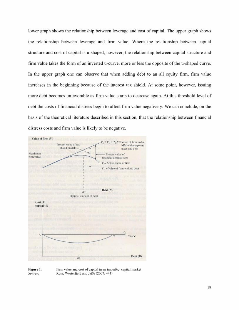
debt, but that taking on too much debt leads to value decreasing financial distress costs. Figure 1

illustrates the effects of taxation and transaction costs on a firm‟s WACC and on firm value. The

6 Modigliani and Miller argue that when a firm attracts more debt it‟s cost of equity rises since the firm becomes

more risky to invest in for equity holders. More debt holders in a firm, namely, means more investors who receive

their money earlier than equity holders, the residual claimants of a firm, when the firm goes bankrupt. The cost of

debt, however, rises very slowly and the fraction of firm value financed with debt increases when a firm attracts

more debt holders. Because more emphasis is put on the relatively low cost of debt, a firm‟s WACC does not change

when a firm increases its usage of debt as a source of funding. Since the WACC does not change when altering the

capital structure of a firm, in a perfect capital market, firm value is also unaffected by a change in capital structure.

The cash flows a firm will earn in the future do not change and neither does the discount rate at which these cash

flows are transformed to present value.

19

lower graph shows the relationship between leverage and cost of capital. The upper graph shows

the relationship between leverage and firm value. Where the relationship between capital

structure and cost of capital is u-shaped, however, the relationship between capital structure and

firm value takes the form of an inverted u-curve, more or less the opposite of the u-shaped curve.

In the upper graph one can observe that when adding debt to an all equity firm, firm value

increases in the beginning because of the interest tax shield. At some point, however, issuing

more debt becomes unfavorable as firm value starts to decrease again. At this threshold level of

debt the costs of financial distress begin to affect firm value negatively. We can conclude, on the

basis of the theoretical literature described in this section, that the relationship between financial

distress costs and firm value is likely to be negative.

Figure 1: Firm value and cost of capital in an imperfect capital market

Source: Ross, Westerfield and Jaffe (2007: 443)

20

§1.3 The opportunity costs of financial distress

In perfectly competitive markets or efficient markets firms cannot make a profit nor are they able

to create value7. Fortunately for firms there are not many markets that approach the definitions of

a perfectly competitive or efficient market. The market descriptions of these markets are mere

extreme exhibits of the direction in which markets tend to move. Nevertheless, it is important to

recognize that not all industries offer equal opportunities for sustained profitability (Porter, 1985:

1). According to Porter (1985: 4) the rules of competition are embodied in five competitive

forces: (1) the entry of new competitors, (2) the threat of substitutes, (3) the bargaining power of

buyers, (4) the bargaining power of suppliers, and (5) the rivalry among the existing competitors.

The collective strength of these five competitive forces will determine the ability of firms to

make a profit or to create value in a market. As the strength of each of these five forces will be

different from market to market, the inherent profitability of markets will also differ from market

to market. Consequently, firms will be able to create more value in markets where the five

competitive forces are favorable than in markets where they are unfavorable. The competitive

forces, however, are dynamical and subject to change. Consequently, when defining competitive

strategy firms should not only focus on being in the right market as to some extent one could also

consider the market a firm operates in as a natural endowment. In contrast, irrespective of the

market a firm operates in, a firm should focus even more on how it can change the competitive

forces in a market to its own favor when defining competitive strategy. In order to be able to

make a profit or to create value a firm should focus on its relative position in the market. Firms

can realize a favorable relative position in a market by creating a sustained competitive

advantage.

7 In Appendix A2 perfectly competitive markets and efficient markets are shortly described.

21

A sustained competitive advantage is a value creating strategy not simultaneously being

implemented by any current or potential competitors who are, above all, unable to duplicate the

benefits of this strategy (Barney, 1991: 206). The indication that a competitive advantage is

sustained does not mean that the specific competitive advantage has eternal life. It does imply

that it will not disappear because of duplication efforts of other firms. Porter (1985: 11) defines

two basic types of competitive advantage a firm can possess: (1) low cost, and (2) differentiation.

Combined with the scope of activities for which firms seek to achieve a competitive advantage

these two types of competitive advantage lead to three generic strategies for achieving a

favorable relative position in a market: (1) cost leadership, (2) differentiation, and (3) focus

(Porter, 1985: 11). Firms use the cost leadership and differentiation strategy to realize a

competitive advantage in many segments of a market, while they use the focus strategy to

acquire cost leadership or differentiation in a more narrow market segment or niche market. In

all strategies firms are effectively trying to influence the five competitive forces in a market to

change them to their favor. In a cost leadership strategy firms try to create barriers to entry by

realizing innovative cost efficient production techniques or by taking over competitors to create

economies of scale. In a differentiation strategy firms try to create barriers to entry by being

unique. Firms may realize the creation of such barriers by producing highly innovative products,

by creating a very strong brand name or by taking over firms that operate in different segments

in the same market in order to be able to offer a unique package of products and services to

buyers. The common characteristic that these strategies share is that the achievement of a

competitive advantage via any strategy requires investments. The ability to invest in investment

opportunities that correspond to a firm‟s strategy is instrumental for a firm wanting to achieve a

competitive advantage. When a firm is in financial distress it does not have the resources

22

available to invest in promising investment opportunities that support the strategy which leads to

a firm‟s ultimate goal: achieving a competitive advantage. The disability to invest can be

interpreted as the opportunity cost of financial distress. Financial flexibility provides firms with

the ability to always have the resources available to invest and, consequently, helps firms to

avoid the opportunity costs of financial distress. Since firms can better execute the actions which

lead to the achievement of a competitive advantage when financially flexible, financial flexibility

is value-creating for firms.

23

Chapter 2 Methodology

At this point, we understand what financial flexibility is and how it theoretically creates value for

firms. In the Introduction we have already defined the two strategies firms can adopt in order to

become financially flexible. We showed that there is strong empirical evidence on a positive

relationship between ‘reducing cash flow volatility’ and firm value. Additionally, we indicated

there is less empirical evidence on the proposed positive relationship between ‘adopting a

conservative capital structure’ and firm value. Consequently, we aim to provide empirical

support on this relationship in this paper. In chapter 2 we describe the methodology we use to

investigate this relationship. First of all, we explain the research design we employed to examine

our main research question. Second, we formulate our main hypotheses. Finally, we define the

data and empirical techniques we make use of in this paper to test our main hypotheses.

§2.1 Research design

We believe we can measure the effect of financial flexibility on firm value by analyzing the

abnormal stock returns of target firms surrounding the period of a leveraged buyout (LBO)

announcement. According to Sudarsanam (2003: 268) a LBO is an acquisition of a corporation

financed mostly with cash, the cash being raised with a preponderance of debt. Almost all LBOs

are transactions where a listed company is acquired and subsequently delisted. Consequently,

they are referred to as public-to-private or going-private transactions (Renneboog and Simons,

2005: 2). According to Renneboog and Simons (2005: 2) virtually all these transactions are

financed by borrowing substantially above the industry average. In general, there are three types

24

of public to private transactions or LBOs: (1) the management buyout (MBO), (2) the

management buyin (MBI), and (3) the institutional buyout (IBO). In a MBO the incumbent

management takes the initiative to take the company private. The funding of the deal is provided

by the management team itself and by private equity investors. In a MBI the company is taken

over by an outside team of managers. Again the funding is provided by the management team

and private equity investors. A LBO is indicated to be an IBO when the new owners of the

delisted firm are solely institutional investors or private equity firms (Renneboog and Simons,

2005: 592).

The market considers LBO‟s as value creating. Substantial premiums are paid for target firms by

acquirers and substantial abnormal returns are observed during the takeover period. Renneboog,

Simons and Wright (2007: 610), for example, find the premiums offered in all UK public-to-

private transactions in the period 1997-2003 to be approximately 41%. The UK evidence is quite

similar to US evidence as Harlow and Howe (1993: 109-118)8 and Travlos and Cornett (1993: 1-

25)9 find the premiums to be 44.9% and 41.9% respectively. In addition, Renneboog, Simons

and Wright (2007: 610) find that the cumulative average abnormal returns (CAARs) surrounding

the announcement of a public-to-private transaction amount to approximately 26% over the event

window [-5,+5] and amount to approximately 29% over the event window [-40,+40] for their

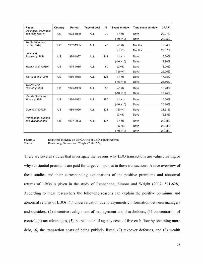
sample of firms. Again there are several studies that obtain similar results for US transactions

(see figure 2).

8 Harlow and Howe (1993: 109-118) examine LBO transactions in the period 1980-1989.

9 Travlos and Cornett (1993: 1-25) examine LBO transactions in the period 1975-1983.

25

Paper Country Period Type of deal N Event window Time event window CAAR

DeAngelo, DeAngelo and Rice (1984) US 1973-1980 ALL 72 (-1,0) Days 22.27%

(-10,+10) Days 28.05%

Torabzadeh and Bertin (1987) US 1982-1985 ALL 48 (-1.0) Months 18.64%

(-1,+1) Months 20.57%

Lehn and Poulsen (1989) US 1980-1987 ALL 244 (-1,+1) Days 16.30%

(-10,+10) Days 19.90%

Marais et al. (1989) US 1974-1985 ALL 80 (0,+1) Days 13.00%

(-69,+1) Days 22.00%

Slovin et al. (1991) US 1980-1988 ALL 128 (-1,0) Days 17.35%

(-15,+15) Days 24.86%

Travlos and Cornett (1993) US 1975-1983 ALL 56 (-1,0) Days 16.20%

(-10,+10) Days 19.24%

Van de Gucht and Moore (1998) US 1980-1992 ALL 187 (-1,+1) Days 15.60%

(-10,+10) Days 20.20%

Goh et al. (2002) US 1980-1996 ALL 323 (-20,+1) Days 21.31%

(0,+1) Days 12.68%

Renneboog, Simons and Wright (2007) UK 1997-2003 ALL 177 (-1,0) Days 22.68%

(-5,+5) Days 25.53%

(-40,+40) Days 29.28%

Figure 2: Empirical evidence on the CAARs of LBO announcements

Source: Renneboog, Simons and Wright (2007: 622)

There are several studies that investigate the reasons why LBO transactions are value creating or

why substantial premiums are paid for target companies in these transactions. A nice overview of

these studies and their corresponding explanations of the positive premiums and abnormal

returns of LBOs is given in the study of Renneboog, Simons and Wright (2007: 591-628).

According to these researchers the following reasons can explain the positive premiums and

abnormal returns of LBOs: (1) undervaluation due to asymmetric information between managers

and outsiders, (2) incentive realignment of management and shareholders, (3) concentration of

control, (4) tax advantages, (5) the reduction of agency costs of free cash flow by obtaining more

debt, (6) the transaction costs of being publicly listed, (7) takeover defenses, and (8) wealth

26

transfers from stakeholders to shareholders. Renneboog, Simons and Wright (2007: 610-619)

conclude that only three of the reasons summed up above can significantly explain the gains

from going private: undervaluation, incentive realignment of management and shareholders and

concentration of control.

In this study we do not intend to explain the gains of LBOs or public-to-private transactions. We

do, however, want to explain why the gains of LBO transactions are larger for some firms than

for other firms. In fact, we use the special character of LBO transactions as a tool to measure the

value of financial flexibility. Since virtually all LBOs are financed with a lot of debt, one may

expect the leverage ratio of the target firm to be much higher and the capital structure of the

target firm to be much less conservative after the transaction. According to Marais et al. (1989:

155) the proportion of debt in the capital structure of the target firm more than triples on average

following a successful buyout. Lehn and Poulsen (1988) present similar results. In addition,

Marais et al. (1989: 155) indicate that most rated debt securities of LBO targets experience

serious downgradings. Warga and Welch (1993: 961) also state that bond ratings of firms

involved in LBOs are usually significantly downgraded. Undergoing a LBO can actually be

interpreted as the opposite of the strategy to achieve financial flexibility we are interested in,

namely adopting a conservative capital structure, as it leads the target firm to adopt a more non-

conservative capital structure. Consequently, the announcement of a leveraged buyout

transaction reveals a target firm‟s financial flexibility is very likely going to deteriorate in the

near future. This deterioration in financial flexibility will have the largest negative impact on

those firms that value financial flexibility the most.

27

The value of financial flexibility for firms heavily depends on a firm‟s need for financial

flexibility. In general, there are two crucial factors that determine a firm‟s need for financial

flexibility: (1) the characteristics of a firm‟s investment opportunities, and (2) a firm‟s cash flow

volatility (Léautier, 2007: 6). The two main characteristics of investment opportunities are timing

and magnitude (Léautier, 2007: 31). Firms that are more regularly confronted with investment

opportunities whose timing is more unpredictable have a higher need for financial flexibility,

since these firms often do not exactly know when they need money to invest in promising

projects, which makes it harder for these firms to match income and expenses. Firms whose

investment opportunities are of a larger magnitude also have a higher need for financial

flexibility, since financing larger investments obviously is more difficult. Consequently, we can

conclude that these firms have a higher need for financial flexibility. The value of financial

flexibility is also larger for these firms as the need for financial flexibility is positively related to

the value of financial flexibility. The cash flow volatility of a firm is the other, next to a firm‟s

investment opportunity characteristics, crucial factor determining a firm‟s need for financial

flexibility. The probability of being confronted with direct and indirect financial distress costs

and the probability of not being able to finance investments when facing adverse cash flow

shocks is higher for firms characterized by a higher cash flow volatility. As a result, the need for

financial flexibility and the value of financial flexibility is also higher for these firms.

Hence, we expect a deterioration in financial flexibility to have the largest negative impact on

those firms characterized by investment opportunities that arise more quickly after one another,

that arise on a more unpredictable pattern and whose magnitude is larger than those of other

firms and on those firms characterized by a higher cash flow volatility. Consequently, we expect

28

the abnormal stock returns of target firms surrounding the period of a leveraged buyout

announcement to be lower for these type of firms.

§2.2 Hypotheses

On the basis of the research design we have just described we are able to formulate our main

hypothesis. In total, we formulate two main hypotheses. In this section we define our hypotheses

accurately and we embed them in the literature.

§2.2.1 The investment opportunity magnitude hypothesis

In the previous section we concluded that firms characterized by investment opportunities that

arise more quickly after one another, that arise on a more unpredictable pattern and whose

magnitude is larger than those of other firms, value financial flexibility more. While this

relationship is a clear one , it is harder to indicate how one should measure the characteristics of

the investment opportunities of firms in order to be able to test whether the relationship

empirically holds. Especially the rate at which a firm gets confronted with investment

opportunities and the unpredictability of investment opportunities seem very hard to measure.

Consequently, we focus on measuring the magnitude of the investment opportunities of firms in

order to be able to test whether the proposed relationship empirically holds. We measure the

magnitude of a firm‟s investment opportunities by four variables: (1) sales growth, (2) capital

expenditures, (3) research and development expenses, and (4) the number of patents or

trademarks a firm possesses. We build upon the real options literature where investments today

are perceived as opportunities to generate returns tomorrow (Luehrman, 1998; Copeland and

29

Antikarov, 2003) to support our methodology of measuring investment opportunities by the

investments firms made in the recent past. First of all, we believe that historical sales growth can

measure the magnitude of a firm‟s investment opportunities as (sales) growth often is a result of

investments made in the past. Pindado and Rodrigues (2005: 348), for example, anticipate that

the investment opportunities of a firm will influence a firm‟s future sales growth. Nash et al.

(2003: 211) find that high investment opportunity firms are characterized by a significantly

higher sales growth than firms with less investment opportunities in a study of the costs and

benefits of restrictive covenants. Del Monte and Papagni (2003: 1003-1014) find the sales

growth rate of firms with R&D expenditures to be higher than that of firms without R&D

expenditures. Second, we believe that the amount of capital expenditures of a firm is a good

measure of the magnitude of a firm‟s investment opportunities. According to John and Mishra

(1989, 837), namely, capital expenditures represent levels of current investment. Additionally,

capital expenditures are purchases of new property, plant and equipment of firms and are

depicted as cash required for investment activities on a firm‟s cash flow statement (Berk and

DeMarzo, 2007: 33). The expenditures can be qualified as investment opportunities since their

goal is to generate positive future cash flows or, in other words, to create value in the future.

Finally, we believe the R&D expenditures of firms and the number of patents or trademarks that

firms possess to be a valid measure of the magnitude of a firm‟s investment opportunities. Nash

et al. (2003: 211), for example, find that high investment opportunity firms are characterized by

significantly higher R&D expenditures than firms with less investment opportunities. In addition,

Gaver and Gaver (1993), Chung and Charoenwong (1991), Gilson (1997) and Skinner (1993)

also measure investment opportunities with R&D expenses. A patent confers firms perfect

appropriability or a monopoly position for a self-developed product for a limited amount of time

30

(Levin et al., 1987: 783). Consequently, because of a patent firms are able to reap the benefits of

R&D activities. As a result, acquiring a patent can be interpreted as an investment of firms to

generate positive returns in the future. According to Landes and Posner (1987: 268) a trademark

is a word, symbol, or other signifier used to distinguish a good or service produced by one firm

from the goods or services of other firms. Consequently, a trademark protects the name a

company has invested in for probably several years on the basis of which it is often able to sell

more of its products than competitors or to sell products at a premium in relation to competitors.

As a result, acquiring a trademark can be interpreted as an investment of firms to generate

positive returns in the future too.

Hypothesis 1: The abnormal returns on a target firm‟s stock during the period surrounding a

LBO announcement are negatively related to the magnitude of a firm‟s investment opportunities,

measured either by sales growth, capital expenditures, research and development expenses, or

the number of patents or trademarks a firm possesses.

The exact hypothesis formulated above has never been tested directly before. There is, however,

some theoretical and indirect evidence. We interpret empirical evidence on the notion that

financial distress costs differ across firms and on the notion that firms incurring the highest

financial distress costs are the least likely to adopt non-conservative capital structures as such

indirect evidence. In a theoretical study Gamba and Triantis (2008: 2263) show that the value of

financial flexibility depends positively on a firm‟s growth potential, which we belief to measure

up to a certain extent by a firm‟s historical sales growth. Bartram et al. (2009: 17), show that

firms who use derivatives are characterized with lower capital expenditures. Since derivative

31

users are likely to have a higher need for financial flexibility, this finding indicates that firms

with a higher need for financial flexibility employ less investment activities measured by a firm‟s

capital expenditures. The finding suggests that firms who have a higher need for financial

flexibility are slowed down in their investment activity by financial inflexibility, which

obviously will affect firm value negatively. Opler and Titman (1994: 1015) find that highly

leveraged firms lose substantial market share to their more conservatively financed competitors

in industry downturns. In addition, Opler and Titman (1994: 1037) show that these indirect

financial distress costs are more pronounced for firms with high R&D expenditures and for firms

operating in more concentrated and more competitive industries. Consequently, Opler and

Titman provide indirect evidence that the value of financial flexibility differs across firms. In

addition, Opler and Titman (1993: 1985) find that firms with high expected costs of financial

distress, i.e. firms characterized by high R&D expenditures, are less likely to undertake

leveraged buyouts. Since a LBO leads to a severe deterioration in a firm‟s capital structure, i.e. a

firm‟s capital structure becomes less conservative because of a LBO, one can interpret the

findings of Opler and Titman as indirect evidence on the notion that certain firms, namely those

firms with high R&D expenditures, are less willing to adopt a non-conservative capital structure

since these firms are characterized by high expected costs of financial distress.

§2.2.2 The cash flow volatility hypothesis

In paragraph 2.1 we concluded that firms characterized by a higher cash flow volatility than

other firms value financial flexibility more. We believe the cash flow volatility of firms can be

measured by the following two variables: (1) the standard deviation of a firm‟s EBITDA over a

recent time period, and (2) the beta coefficient of a firm‟s security. First of all, we believe the

32

standard deviation of a firm‟s EBITDA over a recent time period to be a good measure of a

firm‟s cash flow volatility as EBITDA can be interpreted as a rude measure of a firm‟s cash flow

since it reflects the cash a firm has earned from its operations (Berk and DeMarzo, 2007: 30). In

addition, EBITDA is used in many other empirical studies as estimator variable of a firm‟s true

cash flow (see for example Stein et al., 2001: 100-109, and Kaplan and Zingales, 1997: 169-

215). Second, we believe we can measure a firm‟s cash flow volatility by the beta coefficient of

a firm‟s security. According to Berk and DeMarzo (2007: 308) the beta of a security is the

sensitivity of the security‟s return to the return of the overall market. The beta actually measures

how much of the variability of the return on a firm‟s stock is due to systematic, market-wide

risks (Berk and DeMarzo, 2007: 308). The beta coefficient thus is not an exact measure of a

firm‟s cash flow volatility. However, since the price of a firm‟s security reflects the present value

of the cash flows a firm is expected to generate in the future (Berk and DeMarzo, 2007: 245)

there certainly is a positive relationship between a firm‟s beta coefficient and its cash flow

volatility. The beta coefficient, however, should be interpreted more as the risk on fluctuations

in a firm‟s cash flow due to fluctuations in the business cycle.

Hypothesis 2: The abnormal returns on a target firm‟s stock during the period surrounding a

LBO announcement are negatively related to the cash flow volatility of a firm, measured either

by the standard deviation of a firm‟s EBITDA over a recent time period, or the beta coefficient

of a firm‟s security.

There is no direct empirical evidence that the value of financial flexibility is larger for more

cash-flow volatile firms. In addition, there neither is indirect empirical evidence on this

33

proposed relationship which shows a positive relation between financial distress costs and cash

flow volatility. Shin and Stulz (2000: 20-21), and Allayannis and Weston (2003: 23-24),

however, report a negative relationship between cash flow volatility and shareholder value,

measured among others by price-to-book ratio. In addition, Smithson and Simkins (2005: 13)

report several studies that associate the usage of derivatives contracts, which are instruments that

reduce cash flow volatility, with higher firm values. We belief that the negative relationship

between cash flow volatility and firm value can be explained to a large extent by the positive

relationship between cash flow volatility and financial distress costs. There are theoretical

studies that confirm the positive relation between financial distress costs and cash flow volatility.

Stein et al. (2001: 102), for example, indicate the most important determinant of distress to be

the variability of cash flows. Consequently, we believe the value of financial flexibility to be

higher for firms characterized by a higher cash flow volatility.

§2.3 Data

Now we have formulated our main hypotheses we can start with explaining the method we use to

test our hypotheses. We begin by describing the dataset we gathered on the basis of which we are

able to test the hypotheses. First of all, we will discuss the sample selection procedure. Then, we

will shortly describe the most important descriptive statistics of our dataset.

§2.3.1 Sample selection and data sources

We retrieved all 160 officially disclosed LBO announcements in the United States from October

2006 until September 2009 from the SDC Platinum Worldwide M&A database ( “SDC”), which

provides detailed information on mergers & acquisitions. We focus on the US market solely

34

because of data availability motives. We focus on the time period October 2006 – September

2009 primarily in order to capture the effects of the financial market turmoil or financial credit

crisis which had its most severe impact on the US stock market between October 2007 and

October 2008 (Brunnermeier, 2009: 77). We do realize that data selection out of this specific

time period may bias our results, as financial flexibility is of more worth to firms in financially

unstable times. However, since the goal of this study is examining the value of financial

flexibility to firms, we see no harm in examining it in a period when firms are expected to need it

the most. In addition, although there is evidence of increased takeover activity since mid 2003

(Martynova and Renneboog, 2008: 2152) until summer 2007, the beginning of the credit crisis,

few economists officially, i.e. in published articles, speak of this period as the sixth merger wave.

As the focus of this study is on examining the value of financial flexibility we do not recognize

the added value of examining this value by studying the period of the „sixth merger wave‟ and

thereby adding to the literature on the wealth effects of LBOs. We chose the end date of the time

period we examine, September 2009, because the market index proxy (CRSP equally-weighted

daily returns on the S&P 500 index) we use to conduct our event studies was only available until

December 31, 2009 at the time we conducted the analysis. Since the maximum event window we

use stretches from 60 transaction days before the announcement date to 60 transaction days after

the announcement date, the end date was set 3 months before December 31, 2009. The starting

date of the time period we examine was set exactly 3 years before the end date.

In relation to other mergers and acquisitions a LBO is a special kind of transaction. For some

firms who are eventually taken over via a LBO, the first takeover announcement does not already

reveal the target firm will be taken over via a LBO, but does only reveal there is takeover interest

35

in the target firm. The announcement that the transaction will be a LBO thus follows later. The

SDC database provides information on both announcements and their corresponding dates. In

addition, the SDC database provides a lot of other information about the proposed transaction:

the transaction value, a deal synopsis, information concerning deal characteristics such as

whether the transaction is a MBO or an IBO, whether the bid was perceived as a hostile bid,

whether there was talk of bidder competition, whether the target firm undertook defensive action,

whether the offer was a tender offer and whether the target firm was in financial distress at the

time of the announcement. The SDC database also provides information on the target firm such

as firm activities and accounting information. Since the accounting data available on the target

firms via the SDC database dispose of many missing variables, we gathered most of the

accounting data of the target firms from the COMPUSTAT database which was accessible for us

via Wharton Research Data Services (“WRDS”). We consulted the annual reports of the target

companies when the COMPUSTAT database contained missing variables for specific firms. The

annual reports were accessible for us via the website of the U.S. Securities and Exchange

Commission (“SEC”). The annual reports can be found in the SEC-filings database where they

are indicated as 10-K filings.

We supplemented the data by also gathering share price data of the target firms, information

concerning the ownership structure of the target firms, information concerning R&D

expenditures of the target firms, information on patents and trademarks possessed by the target

firms and the usage of derivatives by the target firms. We gathered the unadjusted share prices of

our target firms from DataStream via the Ticker Codes reported for the target firms in the SDC

database. We downloaded our market index proxy (CRSP equally-weighted daily returns on the

36

S&P 500 index excluding dividends) and the three-month Treasury Bill rate from the CRSP

database which was accessible for us via WRDS. Data on beneficial ownership by management

or by outside shareholders was collected from the target firm‟s last proxy statement prior to the

LBO announcement. The proxy statement is the official notification to shareholders of matters to

be brought to a vote at a company‟s Annual Meeting (Kole, 1995: 416). In the proxy statement a

firm is obligated to indicate security ownership of management and other beneficial owners for

all owners of five percent or more of the firm‟s voting securities (Kole, 1995: 415). The proxy

statements were also accessible for us via the website of the U.S. Securities and Exchange

Commission (after this: “SEC”). They can be found in the SEC-filings database where they are

indicated as DEF 14A filings. Finally, we retrieved information concerning R&D expenditures of

the target firms, the number of patents possessed by the target firms and the usage of derivatives

(interest rate swaps and other derivatives) by the target firms from the annual reports of these

firms. Especially the data we gathered via the annual reports and the proxy statements of the

target firms make our dataset a unique one as these data are not available in any electronic

database. Unfortunately, we had to exclude 9 firms from our sample of 160 firms, because of

divergent reasons. Hence, we retain a sample of 151 firms. First of all, we had to exclude 5

firms10

from our sample due to data unavailability of their stock prices in the time period

surrounding the LBO announcement. Second, we had to remove 4 firms11

from our sample

because of data unavailability of the SEC filings of these firms.

10

The specific firms are RailAmerica Inc., Brand Energy & Infrastructure Services Inc., Sum Total Systems Inc.,

Exotacar Inc. and MSC Software Corp. 11

The specific firms are North Country Hospitality Inc., Maxim Crane Works Holdings Inc., Loring Ward

International Ltd. and Mercari Communications Group Ltd.

37

§2.3.2 Descriptive statistics

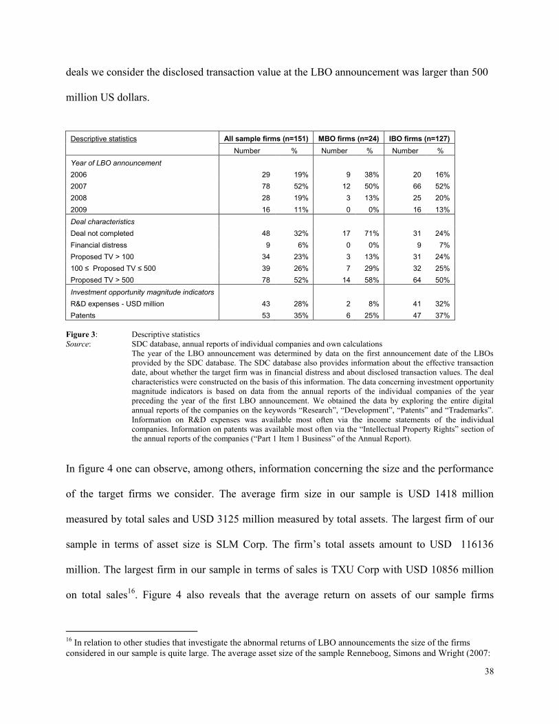
Figure 3 and 4 display instructive descriptive statistics of the proposed LBO transactions we

consider. The goal of showing these statistics is to provide some background information on the

dataset we use on the basis of which we draw important conclusions12

. In figure 3 one can

observe we were only able to distinguish between MBO transactions and IBO transactions on the

basis of the information provided in the deal synopsis of the SDC database13

. In total, our dataset

contains 127 IBOs and 24 MBOs. Additionally, one can observe in the last row of figure 3 that

we do not only consider the announcements of completed LBO deals, but also the

announcements of LBO deals that were not completed14

. Since we focus on explaining the value

of financial flexibility in this study and not on explaining the wealth effects of completed LBO

transactions, we believe that considering the announcements of not completed deals in addition

to the announcements of completed deals does not create bias in our data sample15

. Figure 3 also

shows that most of the announcements we consider took place in the year 2007. The drop in

takeover activity and consequently in LBO activity in 2008 and 2009 can easily be explained by

the credit crisis. Furthermore, one can observe that our sample contains 9 transactions where the

target firm was in financial distress at the time of the announcement. For more than half of the

12

In Appendix B more elaborate descriptive statistics of the dataset we use are depicted. 13

Consequently, we are not able to indicate whether some of the proposed IBO transactions in our sample are

actually MBIs. 14

We can distinguish the not completed deals from the completed deals, since no effective transaction dates are

given for these deals by the SDC database. In the deal synopsis provided by the SDC database this observation is

confirmed as the synopsis reveals a LBO takeover agreement was officially disclosed, but also that it was later

withdrawn. The announcement dates given by the SDC database for these transactions reflect the announcements of

the LBO takeover agreements and not the announcements of the withdrawals. 15

One could argue that not completed deals could be associated with lower abnormal returns as shareholders could

somehow be able to determine the uncertain character of these announced deals. Nevertheless, we test this

relationship in our regression analysis and we are not able to find a significant negative or positive relationship

between the abnormal returns of the LBO announcements we consider and a dummy variable for not completed

deals. In addition, the cumulative abnormal returns for target firms of completed and non-completed deals are quite

similar. In Appendix E the test and the comparison we just described are depicted.

38

deals we consider the disclosed transaction value at the LBO announcement was larger than 500

million US dollars.

Descriptive statistics All sample firms (n=151) MBO firms (n=24) IBO firms (n=127)

Number % Number % Number %

Year of LBO announcement

2006 29 19% 9 38% 20 16%

2007 78 52% 12 50% 66 52%

2008 28 19% 3 13% 25 20%

2009 16 11% 0 0% 16 13%

Deal characteristics

Deal not completed 48 32% 17 71% 31 24%

Financial distress 9 6% 0 0% 9 7%

Proposed TV > 100 34 23% 3 13% 31 24%

100 ≤ Proposed TV ≤ 500 39 26% 7 29% 32 25%

Proposed TV > 500 78 52% 14 58% 64 50%

Investment opportunity magnitude indicators

R&D expenses - USD million 43 28% 2 8% 41 32%

Patents 53 35% 6 25% 47 37%

Figure 3: Descriptive statistics

Source: SDC database, annual reports of individual companies and own calculations

The year of the LBO announcement was determined by data on the first announcement date of the LBOs

provided by the SDC database. The SDC database also provides information about the effective transaction

date, about whether the target firm was in financial distress and about disclosed transaction values. The deal

characteristics were constructed on the basis of this information. The data concerning investment opportunity

magnitude indicators is based on data from the annual reports of the individual companies of the year

preceding the year of the first LBO announcement. We obtained the data by exploring the entire digital

annual reports of the companies on the keywords “Research”, “Development”, “Patents” and “Trademarks”.

Information on R&D expenses was available most often via the income statements of the individual

companies. Information on patents was available most often via the “Intellectual Property Rights” section of

the annual reports of the companies (“Part 1 Item 1 Business” of the Annual Report).

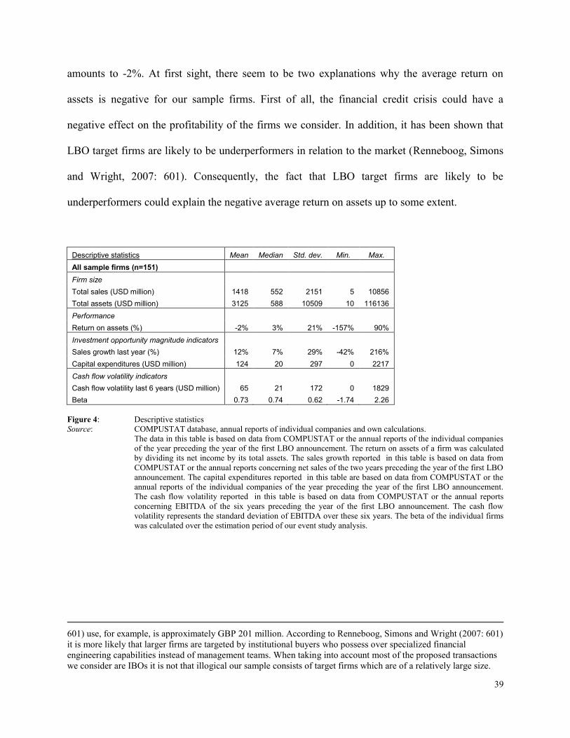
In figure 4 one can observe, among others, information concerning the size and the performance

of the target firms we consider. The average firm size in our sample is USD 1418 million

measured by total sales and USD 3125 million measured by total assets. The largest firm of our

sample in terms of asset size is SLM Corp. The firm‟s total assets amount to USD 116136

million. The largest firm in our sample in terms of sales is TXU Corp with USD 10856 million

on total sales16

. Figure 4 also reveals that the average return on assets of our sample firms

16

In relation to other studies that investigate the abnormal returns of LBO announcements the size of the firms

considered in our sample is quite large. The average asset size of the sample Renneboog, Simons and Wright (2007:

39

amounts to -2%. At first sight, there seem to be two explanations why the average return on

assets is negative for our sample firms. First of all, the financial credit crisis could have a

negative effect on the profitability of the firms we consider. In addition, it has been shown that

LBO target firms are likely to be underperformers in relation to the market (Renneboog, Simons

and Wright, 2007: 601). Consequently, the fact that LBO target firms are likely to be

underperformers could explain the negative average return on assets up to some extent.

Descriptive statistics Mean Median Std. dev. Min. Max.

All sample firms (n=151)

Firm size

Total sales (USD million) 1418 552 2151 5 10856

Total assets (USD million) 3125 588 10509 10 116136

Performance

Return on assets (%) -2% 3% 21% -157% 90%

Investment opportunity magnitude indicators

Sales growth last year (%) 12% 7% 29% -42% 216%

Capital expenditures (USD million) 124 20 297 0 2217

Cash flow volatility indicators

Cash flow volatility last 6 years (USD million) 65 21 172 0 1829

Beta 0.73 0.74 0.62 -1.74 2.26

Figure 4: Descriptive statistics

Source: COMPUSTAT database, annual reports of individual companies and own calculations.

The data in this table is based on data from COMPUSTAT or the annual reports of the individual companies

of the year preceding the year of the first LBO announcement. The return on assets of a firm was calculated

by dividing its net income by its total assets. The sales growth reported in this table is based on data from

COMPUSTAT or the annual reports concerning net sales of the two years preceding the year of the first LBO

announcement. The capital expenditures reported in this table are based on data from COMPUSTAT or the

annual reports of the individual companies of the year preceding the year of the first LBO announcement.

The cash flow volatility reported in this table is based on data from COMPUSTAT or the annual reports

concerning EBITDA of the six years preceding the year of the first LBO announcement. The cash flow

volatility represents the standard deviation of EBITDA over these six years. The beta of the individual firms

was calculated over the estimation period of our event study analysis.

601) use, for example, is approximately GBP 201 million. According to Renneboog, Simons and Wright (2007: 601)

it is more likely that larger firms are targeted by institutional buyers who possess over specialized financial

engineering capabilities instead of management teams. When taking into account most of the proposed transactions

we consider are IBOs it is not that illogical our sample consists of target firms which are of a relatively large size.

40

Finally, figure 3 and 4 report information about the magnitude of the investment opportunities

and about the cash flow volatility of the target firms in our sample, which are, in fact, the most

important variables in our analysis as it are key inputs for testing our hypotheses. One can

observe in figure 4 that the average sales growth, measured over the two years preceding the year

of the (first) LBO announcement, of our target firms was 12%. Although we cannot compare this

number to firms that were not involved in a LBO takeover process, the number seems rather

high. The high growth in sales observed among the firms in our sample suggests high growth

firms are more likely targets for LBOs. In addition, figure 4 indicates average capital

expenditures to be USD 124 million, average cash flow volatility over the 6 years preceding the

year of the (first) LBO announcement to be USD 65 million and an average beta coefficient of

0.73 for our sample firms. The average beta coefficient observed is lower than one, which

indicates the stock returns of our sample firms are less prone to swings in the business cycle than

the average firm. Figure 3 shows how many firms in our sample spend money on research and

development and how many firms possess patents or trademarks. One can observe that 43 firms

in our sample have positive R&D expenses and 53 firms in our sample possess patents or

trademarks. The firms that have positive R&D expenses often do also possess patents or

trademarks, which is not surprising as patents and trademarks are only filed for when serious

research and development activity has taken place already. In total, 67 of the firms in our sample

have positive R&D expenses or possess patents or trademarks. 84 of the firms in our sample do

not spend money on R&D nor do they possess patents or trademarks.

41

§2.4 Empirical techniques

In the previous section we described the data selection procedure, we described the different data

sources we have used in order to gather our data and we provided some informative descriptive

statistics of our dataset. In this section we describe the empirical techniques we used to analyze

the data we gathered in order to test whether the hypotheses we formulated in section 2.2

empirically hold. We employed two empirical techniques for our data analysis: (1) event studies,

and (2) cross-sectional regression analysis. In this section we will explain both techniques more

extensively.

§2.4.1 Event study

We examine the effect of a LBO announcement on firm value in the light of financial flexibility,

among others, by using the event study methodology. An event study measures the impact of a

specific event on the value of a firm using financial market data (MacKinlay, 1997: 13). The

usefulness of event studies leans heavily on the hypothesis that stock markets are rational and

consequently that the impact of events is immediately reflected in stock market prices. The event

study methodology has been frequently used in the corporate finance literature concerning

mergers and acquisitions. As a result, the methodology can well be used to analyze the effect of a

LBO announcement on firm value in the light of financial flexibility.

We identify two events for LBO transactions: (1) the first announcement of takeover interest in

the target firm, and (2) the first announcement that the type of deal is a LBO17

. In general, event

17

Defining the event of interest is non-standard for LBO‟s in relation to other mergers or acquisitions as a LBO is a

special kind of transaction. For some firms who are eventually taken over via a LBO, the first takeover

42

1 and event 2 coincide for some LBO announcements, and do not coincide for others18

. We

examine five event windows, i.e. the period over which the stock market returns on the securities

of the firms examined are observed: (1) one trading day before the event to one trading day after

the event [-1,+1], (2) five trading days before the event to five trading days after the event [-

5,+5], (3) twenty trading days before the event to twenty trading days after the event [-20,+20],

(4) forty trading days before the event to forty trading days after the event [-40,+40], and (5)

sixty trading days before the event to sixty trading days after the event [-60,+60]. In order to

determine abnormal returns in the event window, one has to define a measure of normal returns.

We choose a CAPM type model to measure normal returns: ( ). One

needs to identify an estimation window to measure the of the CAPM type model in order to

be able to construct the measure of normal returns in the event window. We use an estimation

window that starts 317 trading days before event 1 and that ends 66 trading days before event 1.

Finally, we define the measure of abnormal return as the actual return on a firm‟s stock during

the event window minus the normal return on a firm‟s stock during the event window:

19.

announcement does not already reveal the target firm will be taken over via a LBO, but does only announce there is

takeover interest in the target firm (Renneboog, Simons and Wright, 2007: 608). The announcement that the

transaction will be a LBO thus follows later. 18

For 87% of the firms (i.e. 132) in our sample event1 and event 2 coincide. Consequently, 13% (i.e. 19) of the

LBO announcements of our sample firms are, in fact, two announcements: an announcement of takeover interest and

an announcement that the proposed transaction is a LBO. In order to be able to compare the abnormal returns of

these two groups of LBO announcement target firms, we added the abnormal returns of event 1 and event 2 for the

group of firms characterized by 2 event dates in order to make them better comparable to the group of firms

characterized by 1 event date. Naturally, we excluded overlap in the event windows of event 1 and event 2 for the

first group of firms. 19

In Appendix C1 the event study methodology we use is described more elaborately.

43

§2.4.2 Cross-sectional regression analysis

Remember that we hypothesized in section 2.2 we expect the abnormal returns of target firms

during the period in which a LBO announcement is made to be negatively related to the

magnitude of a firm‟s investment opportunities and a firm‟s cash flow volatility. In this section

we explain how we intend to test these hypotheses. We test the two main hypotheses formulated

in section 2.2 by estimating a cross-sectional regression using the cumulative abnormal returns of

our smallest event window, CAR[-1,+1], as main dependent variable20

. We use the CAR

measured over the smallest event window as dependent variable, since we feel this number

measures the abnormal returns of LBO announcements most precisely. We use the four

indicators of the magnitude of investment opportunities of firms (sales growth, capital

expenditures, research and development expenses and the number of patents or trademarks a firm

possesses) and the two indicators of the cash flow volatility of firms (the standard deviation of a

firm‟s EBITDA over a recent time period and the beta coefficient of a firm‟s security), also

discussed in section 2.2, as main independent variables. In addition, we include several control

variables as our main independent variables are not likely to be the only variables explaining the

variation in our dependent variable21

. In total, we distinguish four groups of relevant control

variables: (1) factors explaining the gains from going private, (2) factors indicating leverage,

20

The calculation of the CAR measure is explained in Appendix C3. 21

Multiple regression analysis allows us to explicitly control for many other factors than our main independent

variables that simultaneously affect the dependent variable (Wooldridge, 2006: 73). Including all the relevant

variables that might affect the dependent variable is crucial as it improves the explanatory power of the regression

model and prevents underspecification of the model. Underspecification should be prevented as it causes the

coefficients in an ordinary least squares (after this: “OLS”) regression to be biased. The bias caused by

underspecification is also known as the omitted variable bias (Wooldridge, 2006: 73). On the other hand, we should

also be wary of including too many independent variables or overspecifying the model, since this would cause

multicollinearity. Multicollinearity can be described as a high, but not perfect, correlation between two or more

independent variables (Wooldridge, 2006: 102). Multicollinearity leads to higher variances for the OLS estimators

of the coefficients of independent variables (Wooldridge, 2006: 73). As a result, the OLS estimators become less

efficient.

44

(3) derivatives, and (4) other control variables. We will now describe the four groups of control

variables more extensively.

Factors explaining the gains from going private

In section 2.1, where we described our research design, we showed that according to Renneboog,

Simons and Wright (2007: 595-600) there are, in essence, 8 reasons that explain the wealth gains

of going-private. We also pointed out that Renneboog, Simons and Wright (2007: 610-619)

conclude that only three of these reasons can significantly explain the gains from going private:

undervaluation, incentive realignment of management and shareholders and concentration of

control. Consequently, we choose to only incorporate these 3 reasons as explanatory control

variables in our cross-sectional regression and to not test for the other 5 reasons22

. First of all,

undervaluation due to asymmetric information between managers and outsiders might explain

the gains of going private. Managers may believe the share price of a firm is undervalued relative

to the potential they believe the firm to have based on superior private information. When listed

firms have difficulties for fund expansion and when their shares can be characterized as illiquid

or as thinly traded, the prospect that the firm‟s shares will remain to be lowly valued might be a

rationale for firms to go private (Renneboog, Simons and Wright, 2007: 599). We examine the

undervaluation hypothesis by including the average share price returns of the target firms we

22

The other 5 reasons are: (1) tax advantages, (2) the reduction of agency costs of free cash flow by obtaining more

debt, (3) the transaction costs of being publicly listed, (4) takeover defenses, and (5) wealth transfers from

stakeholders to shareholders. We do actually test for tax advantages and the reduction of agency costs of free cash

flow as explanatory variables of the wealth gains of going private by including the taxes paid and the EBITDA of

our target firms as independent variables in our cross-sectional regression. However, because we neither find a

significant relationship between these two variables and CAR[-1,+1], we choose not to include these variables as

independent variables in our regression. Additionally, the transaction costs of being publicly listed, takeover

defenses and wealth transfers from stakeholders to shareholders might explain the gains from going private. Because

of the difficulty to collect the data needed to test these last three hypotheses and the expectation that all of them will

not exhibit significant relationships with our main dependent variable, we choose not to test for these hypotheses.

45

consider measured in the estimation window of our event study analysis as an independent

variable23

. Second, incentive realignment of management and shareholders might explain the

gains of going private because potential agency problems are expected to be reduced in buyouts

(Renneboog, Simons and Wright, 2007: 618). Managers who are also the owners of a firm

extract pecuniary and non-pecuniary benefits from the firm they own. When the share of

ownership of these managers decreases in a company they will extract even more of such private

benefits as they have to bear a smaller fraction of the costs that accompany such extraction.

Consequently, firms whose managers own only a small stake in the firm‟s equity will benefit

more from a LBO. We examine the incentive realignment hypothesis24

by including the highest

managerial equity stake of the target firms we consider as an independent variable25

. Third,

concentration of control might explain the gains of going private because a LBO can increase the

degree of monitoring in firms with a dispersed ownership structure as the buyout often leads to

fewer owners in such firms. Grossman and Hart (1980) show that public corporations often

suffer from a lack of monitoring because of a dispersed ownership structure where all the owners

free-ride on each other concerning the monitoring of managers. Consequently, we expect higher

gains from going-private for firms who have smaller (in percentages of shares owned) outside

monitoring shareholders or blockholders. We examine the concentration of control hypothesis26

by including the highest outside blockholder equity stake of the target firms we consider as an

23

Renneboog, Simons and Wright (2007: 617) find a significant negative relationship between the share price

returns over a one-year period ending 1 month before the first LBO announcement and the CAARs measured during

a short period surrounding the LBO announcement. 24

Renneboog, Simons and Wright (2007: 616) find a significant negative relationship between managerial equity

ownership in the pre-transaction firm and the CAARs measured during a short period surrounding the LBO

announcement. 25

We choose to use the highest managerial equity stake and not the total managerial equity stake in order to exclude

small ownership stakes of managers from the analysis. 26

Renneboog, Simons and Wright (2007: 616) find a significant negative relationship between the presence of

institutional or corporation blockholders with stakes larger than 5% in the pre-transaction firm and the CAARs

measured during a short period surrounding the LBO announcement.

46

independent variable27

. In addition, we include 5 dummy variables to indicate the type of

blockholder as certain blockholders are expected to monitor more than others: (1) individual, (2)

company, (3) bank, insurance company or pension fund, (4) investor group or private equity

investor, and (5) trust fund (often established by or for employees).

Factors indicating leverage

In chapter one we showed that higher debt levels are associated with higher costs of financial

distress. Consequently, the abnormal returns of LBO announcements might be negatively related

to the debt levels or leverage of firms as these firms are likely to have a higher need for financial

flexibility and consequently are likely to value financial flexibility more. In order to control for

this possible relationship, we include 5 control variables. First of all, we include the four factors

explaining leverage according to the influential empirical study of Rajan and Zingales (1995):

tangibility of assets, market-to-book ratio, firm size and profitability28

. We limit ourselves to

these variables as they have shown up most consistently in previous studies as being correlated

with leverage (Rajan and Zingales, 1995: 1451)29

. In addition, we include the ratio of debt, i.e.

the sum of current liabilities and long-term debt, to total assets in our regression as a control

variable.

27

We choose to use the highest equity stake and not the total equity stake in order to exclude small ownership stakes

from the analysis and in order to capture that blockholder who has the largest incentive to monitor. 28

We include the tangible assets, the total sales and the EBIT of our target firms in our regression as control

variables. In addition, we include the market value to total assets in our regression as a control variable. Although

this ratio does not precisely measure the market-to-book ratio, where market value is divided by stockholder‟s

equity, we decided to use market value to total assets because of some negative stockholder‟s equity values observed

among some of our sample firms. 29

According to Rajan and Zingales (1995) tangibility of assets and size correlate positively with leverage, and

market-to-book ratio and profitability correlate negatively with leverage. In appendix A3 we explain the

relationships between leverage and tangibility of assets, market-to-book ratio, firm size and profitability more

elaborately.

47

Derivatives

We belief there is a positive relationship between the usage of derivatives of target firms and the

abnormal returns of LBO announcements. Firms use derivatives, among others to decrease their

cash flow volatility. Consequently, these firms will have a lower need for financial flexibility

established via adopting a conservative capital structure. As a result, we expect higher abnormal

returns for firms who use derivatives than for firms who do not use derivatives. The fact that a

firm uses derivatives, however, might also indicate that the firm suffers from high cash flow

volatility. The abnormal returns might therefore also be lower for derivative users. We measure

derivative usage by two dummy variables: one dummy variable measures whether a company

uses interest rate swaps or not, and the other dummy variable measures whether a company uses

derivatives other than interest rate swaps or not.

Other control variables

Finally, we include a MBO dummy variable and a financial distress dummy variable as control

variables. The MBO dummy indicates whether the proposed deal is a management buyout. We

expect the relationship between the MBO dummy and the CARs to be positive as a higher

ownership stake for management (not too high however) alleviates agency problems in the

company. The financial distress dummy indicates whether the target company is financially

distressed or not. We expect the relationship between this dummy variable and the CARs to be

negative, among others, because more debt is likely to have an adverse effect on the financial

flexibility and, consequently, on the value of these firms.

48

Chapter 3 Results

In chapter 2 we discussed the research design we use in this paper and we formulated our main

hypotheses. In addition, we described the dataset and the empirical techniques we use to test our

hypotheses. In this chapter we present the results of the data analysis procedures we employed.

First of all, we present the results of the event study. Second, we depict the results of the cross-

sectional regression analysis.

§3.1 Event study

The cumulative average abnormal returns (CAARs) of the LBO announcements for our entire

sample of target firms are depicted in figure 5. One can observe that the CAAR over the event

window [-1,+1] amounts to 22.94% for all our sample firms and increases to 30.63% for the

largest event window considered [-60,+60]. We also depict the CAARs of all our sample firms

for the event window [-5,+5] graphically in figure 6. One can observe in figure 2, depicted in

paragraph 2.1, that these results are quite comparable to previous empirical evidence on the

CAARs of LBO announcements. In addition, we find that the CAARs are different from zero at

the 1% significance level for all event windows30

, which is also comparable to previous

empirical evidence on the CAARs of LBO announcements. The fact that the results we obtain for

our event study are in line with the results of previous studies leads us to conclude we performed

the event study analysis correctly.

30

In appendix C2 and C3 the event study results and the empirical tests we run on these results are treated more

elaborately.

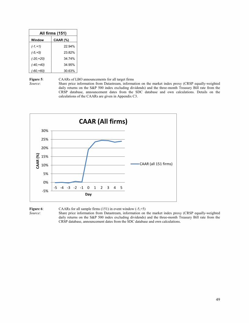
49

All firms (151)

Window CAAR (%)

(-1,+1) 22.94%

(-5,+5) 23.82%

(-20,+20) 34.74%

(-40,+40) 34.95%

(-60,+60) 30.63%

Figure 5: CAARs of LBO announcements for all target firms

Source: Share price information from Datastream, information on the market index proxy (CRSP equally-weighted

daily returns on the S&P 500 index excluding dividends) and the three-month Treasury Bill rate from the

CRSP database, announcement dates from the SDC database and own calculations. Details on the

calculations of the CAARs are given in Appendix C3.

Figure 6: CAARs for all sample firms (151) in event window (-5,+5)

Source: Share price information from Datastream, information on the market index proxy (CRSP equally-weighted

daily returns on the S&P 500 index excluding dividends) and the three-month Treasury Bill rate from the

CRSP database, announcement dates from the SDC database and own calculations.

-5%

0%

5%

10%

15%

20%

25%

30%

-5 -4 -3 -2 -1 0 1 2 3 4 5

CA

AR

(%

)

Day

CAAR (All firms)

CAAR (all 151 firms)

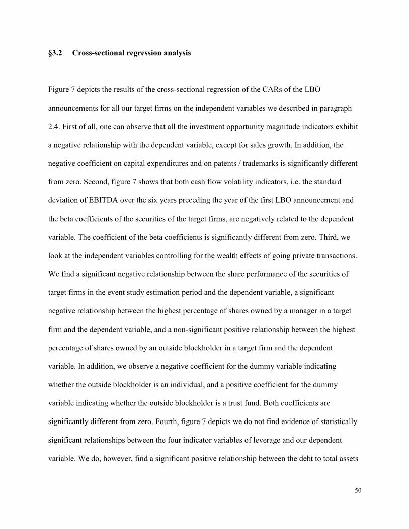
50

§3.2 Cross-sectional regression analysis

Figure 7 depicts the results of the cross-sectional regression of the CARs of the LBO

announcements for all our target firms on the independent variables we described in paragraph

2.4. First of all, one can observe that all the investment opportunity magnitude indicators exhibit

a negative relationship with the dependent variable, except for sales growth. In addition, the

negative coefficient on capital expenditures and on patents / trademarks is significantly different

from zero. Second, figure 7 shows that both cash flow volatility indicators, i.e. the standard

deviation of EBITDA over the six years preceding the year of the first LBO announcement and

the beta coefficients of the securities of the target firms, are negatively related to the dependent

variable. The coefficient of the beta coefficients is significantly different from zero. Third, we

look at the independent variables controlling for the wealth effects of going private transactions.

We find a significant negative relationship between the share performance of the securities of

target firms in the event study estimation period and the dependent variable, a significant

negative relationship between the highest percentage of shares owned by a manager in a target

firm and the dependent variable, and a non-significant positive relationship between the highest

percentage of shares owned by an outside blockholder in a target firm and the dependent

variable. In addition, we observe a negative coefficient for the dummy variable indicating

whether the outside blockholder is an individual, and a positive coefficient for the dummy

variable indicating whether the outside blockholder is a trust fund. Both coefficients are

significantly different from zero. Fourth, figure 7 depicts we do not find evidence of statistically

significant relationships between the four indicator variables of leverage and our dependent

variable. We do, however, find a significant positive relationship between the debt to total assets

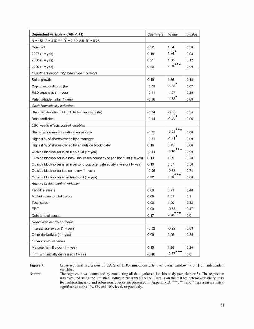
51

Dependent variable = CAR(-1,+1) Coefficient t-value p-value

N = 151; F = 3.07***; R2 = 0.39; Adj. R

2 = 0.26

Constant 0.22 1.04 0.30

2007 (1 = yes) 0.18 1.74* 0.08

2008 (1 = yes) 0.21 1.58 0.12

2009 (1 = yes) 0.59 3.69*** 0.00

Investment opportunity magnitude indicators

Sales growth 0.19 1.36 0.18

Capital expenditures (ln) -0.05 -1.86* 0.07

R&D expenses (1 = yes) -0.11 -1.07 0.29

Patents/trademarks (1=yes) -0.16 -1.73* 0.09

Cash flow volatility indicators

Standard deviation of EBITDA last six years (ln) -0.04 -0.95 0.35

Beta coefficient -0.14 -1.88* 0.06

LBO wealth effects control variables

Share performance in estimation window -0.05 -3.23*** 0.00

Highest % of shares owned by a manager -0.51 -1.71* 0.09

Highest % of shares owned by an outside blockholder 0.16 0.45 0.66

Outside blockholder is an individual (1= yes) -0.34 -3.16*** 0.00

Outside blockholder is a bank, insurance company or pension fund (1= yes) 0.13 1.09 0.28

Outside blockholder is an investor group or private equity investor (1= yes) 0.10 0.67 0.50

Outside blockholder is a company (1= yes) -0.06 -0.33 0.74

Outside blockholder is an trust fund (1= yes) 0.92 4.45*** 0.00

Amount of debt control variables

Tangible assets 0.00 0.71 0.48

Market value to total assets 0.05 1.01 0.31

Total sales 0.00 1.00 0.32

EBIT 0.00 -0.73 0.47

Debt to total assets 0.17 2.78*** 0.01

Derivatives control variables

Interest rate swaps (1 = yes) -0.02 -0.22 0.83

Other derivatives (1 = yes) 0.09 0.95 0.35

Other control variables

Management Buyout (1 = yes) 0.15 1.28 0.20

Firm is financially distressed (1 = yes) -0.46 -2.57*** 0.01

Figure 7: Cross-sectional regression of CARs of LBO announcements over event window [-1,+1] on independent

variables.

Source: The regression was computed by conducting all data gathered for this study (see chapter 3). The regression

was executed using the statistical software program STATA. Details on the test for heteroskedasticity, tests

for multicollinearity and robustness checks are presented in Appendix D. ***, **, and * represent statistical

significance at the 1%, 5% and 10% level, respectively.

52

ratio of the target firms and the dependent variable. Fifth, one can observe positive and

statistically significant coefficients for the dummy variables indicating whether the LBO

announcement took place in 2007 and 2009. Furthermore, one can observe we do not find a

statistically significant relationship between the dependent variable and one of the derivative

control variables, nor do we find such a relationship between the dependent variable and the

management buyout dummy variable. Finally, we do find a negative coefficient for the dummy

variable indicating whether a target company was in financial distress at the time of the LBO

announcement, which is significantly different from zero.

We test our main cross-sectional regression for heteroskedasticity by means of a White test

(White, 1980). We do not find evidence of heteroskedasticity. In addition, we test our regression

for multicollinearity. We use a correlation matrix, variance inflation factors and the condition

number computed by means of eigenvalues in order to detect multicollinearity. We, however, do

not find strong evidence of multicollinearity. Finally, we also check the robustness of our

regression, by also using CARs of wider event windows as dependent variable. We find that the

significant negative relationships between capital expenditures and cumulative abnormal returns,

and between patents or trademarks and cumulative abnormal returns continue to hold and even

become more significant when widening the event window to CAAR[-10,+10]. When widening

the window further the relationships do not hold anymore. The negative significant relationship

between the beta coefficient and the cumulative abnormal returns immediately becomes

insignificant when widening the event window. We can conclude that the results we obtain

depend on the narrowness of the event window used to examine cumulative abnormal returns.

53

We belief this is not an odd observation, as smaller event windows capture the effect of the event

more precisely since less noise will be incorporated31

.

31

All the tests are described more elaborately in Appendix D.

54

Chapter 4 Discussion

In the Introduction we formulated our main research question and we motivated why the topic of

this thesis is interesting. On the basis of the theoretical background discussed, among others, in

chapter 1 we formulated our main hypotheses in chapter 2. Subsequently, we described the

methodology with the help of which we test these hypotheses. In the last chapter we presented the

results. In this chapter we discuss the meaning and the implications of the results presented in

the previous chapter. In addition, we link the results obtained to previous empirical evidence

earlier discussed in this paper.

Remember the two main hypotheses we formulated in chapter 2. In fact, we build upon two

assumptions when we formulated these hypotheses: (1) the value of financial flexibility is

highest for those firms who have a higher need for financial flexibility (Léautier, 2007: 6), and

(2) the announcement of a leveraged buyout transaction reveals a target firm‟s financial

flexibility is very likely going to deteriorate in the near future. On the basis of these two basic

assumptions we expected the abnormal returns on a target firm‟s stock during the period

surrounding a LBO announcement to be negatively related to the magnitude of a firm‟s

investment opportunities (measured either by sales growth, capital expenditures, research and

development expenses, or the number of patents or trademarks a firm possesses) and to the cash

flow volatility of a firm (measured either by the standard deviation of a firm‟s EBITDA over a

recent time period, or the beta coefficient of a firm‟s security). We will now discuss whether

these expectations have all been confirmed by or results and whether this is explicable or not.

First of all, we will discuss the results that can be associated with the investment opportunity

55

magnitude hypothesis. Second, we treat the meaning and implications of the results that can be

associated with the cash flow volatility hypothesis. Finally, we will address some other

interesting results our cross-sectional regression has produced.

§4.1 The investment opportunity magnitude hypothesis

In chapter 3 we showed that all the investment opportunity magnitude indicators exhibit a

negative relationship with the dependent variable in the cross-sectional regression we run, except

for sales growth. In addition, we showed the negative coefficient on capital expenditures and on

patents / trademarks is significantly different from zero. Consequently, the evidence on a

negative relationship between the abnormal returns on a target firm‟s stock during the period

surrounding a LBO announcement and capital expenditures and the possession of patents and / or

trademarks is most convincing.

First of all, we motivated capital expenditures to be a good measure of the magnitude of a firm‟s

investment opportunities in paragraph 2.2 by, among others, the notion of John and Mishra

(1989, 837) that capital expenditures represent current levels of investment. In addition, we

provided indirect empirical evidence on the assumed positive relationship between the amount of

capital expenditures of a firm and the value of financial flexibility. We interpreted evidence of

Bartram et al. (2009: 17), who show that firms who use derivatives are characterized with lower

capital expenditures, as indirect evidence on the notion that firms who have a higher need for

financial flexibility (derivative users) are slowed down in their investment activity by financial

inflexibility, which will affect their firm value negatively. Our finding on the negative

56

relationship between capital expenditures and the abnormal returns of target firm‟s securities

during a LBO announcement confirms this interpretation to some extent. In addition, it provides

more direct evidence on the assumed positive relationship between the amount of capital

expenditures of a firm and the value of financial flexibility. Second, we motivated the amount of

patents or trademarks a firm possesses to be a good measure of the magnitude of a firm‟s

investment opportunities in paragraph 2.2 by arguing that acquiring a patent or trademark is

primarily done by firms to reap the future benefits of previous investments made, for example

investments made in R&D activities or in a brand name. In addition, we provided indirect

empirical evidence on the assumed positive relationship between the amount of patents or

trademarks a firm possesses and the value of financial flexibility. We interpret evidence of Opler

and Titman (1994: 1037), who show that indirect financial distress costs are more pronounced

for firms with high R&D expenditures and for firms operating in more concentrated and more

competitive industries, as such indirect evidence as we also expect patents and trademarks to be a

more important ingredient of business in these industries. Our finding on the negative

relationship between the amount of patents or trademarks a firm possesses and the abnormal

returns of target firm‟s securities during a LBO announcement confirms this interpretation to

some extent. In addition, it provides more direct evidence on the assumed positive relationship

between the amount of patents or trademarks a firm possesses and the value of financial

flexibility. Third, we motivated the research and development expenses of firms to be a good

measure of the magnitude of a firm‟s investment opportunities in paragraph 2.2 by, among

others, citing the finding of Nash et al. (2003: 211) that high investment opportunity firms are

characterized by significantly higher R&D expenditures than firms with less investment

opportunities. In addition, we provided indirect empirical evidence on the assumed positive

57

relationship between the research and development expenses of firms and the value of financial

flexibility. We interpret evidence of Opler and Titman (1993: 1985), who find that firms with

high expected costs of financial distress, i.e. firms characterized by high R&D expenditures, are

less likely to undertake leveraged buyouts, as such indirect evidence. Our finding on the negative

relationship between the research and development expenses of firms and the abnormal returns

of target firm‟s securities during a LBO announcement provides more direct evidence on the

assumed positive relationship between the amount of R&D expenditures of a firm and the value

of financial flexibility. The finding, however, is less strong than the finding for capital

expenditures and patents or trademarks. An explanation might be that R&D expenses measure

investment opportunities too specifically, i.e. only for high-tech firms, and neglect the

investments of less technology-oriented companies which are measured by capital expenditures

or patents and / or trademarks. Finally, we motivated the (historical) sales growth of firms to be

a good measure of the magnitude of a firm‟s investment opportunities in paragraph 2.2 by,

among others, citing the finding of Nash et al. (2003: 211) that high investment opportunity

firms are characterized by a significantly higher sales growth than firms with less investment

opportunities. In addition, we provided theoretical evidence on the assumed positive relationship

between sales growth and the value of financial flexibility by quoting the study of Gamba and

Triantis (2008). In this study Gamba and Triantis (2008: 2263) show that the value of financial

flexibility depends positively on a firm‟s growth potential, which we belief to measure up to a

certain extent by a firm‟s historical sales growth. We, however, cannot support the hypotheses by

the results of our cross sectional regression as we find a positive relationship between sales

growth and the abnormal returns of target firm‟s securities during a LBO announcement. An

explanation might be that the sales growth measure we use represents the potential of a firm to

58

grow rather than the magnitude of its investment opportunities. When assuming that LBO target

firms are underperformers as shortly discussed in paragraph 2.3 sales growth might measure for

the potential to reorganize a firm and make it profitable again by cutting its operating costs and

increasing its sales. To a certain extent this finding would support the notion of Jensen (1980)

that private equity firms, who are often involved in LBO transactions, bring financial,

governance and operational engineering to a company and will therefore ameliorate a company‟s

operating performance and consequently create value. The positive coefficient could also

indicate that investors value young and emerging firms, often targeted by venture capitalist firms

(Kaplan and Strömberg, 2009: 121), who first did not appear clearly but who have just begun to

make progression, more.

§4.2 The cash flow volatility hypothesis

In chapter 3 we showed that all the cash flow volatility indicators exhibit a negative relationship

with the dependent variable in the cross-sectional regression we run. In addition, we showed the

negative coefficient on the beta coefficient is significantly different from zero, but that the

negative coefficient on the standard deviation of EBITDA is not. Consequently, the evidence on

a negative relationship between the abnormal returns on a target firm‟s stock during the period

surrounding a LBO announcement and the beta coefficient is most convincing.

First of all, we motivated the beta coefficient of a firm‟s security to be a good measure of a

firm‟s cash flow volatility in paragraph 2.2 by arguing it can actually be interpreted as the risk

on fluctuations in a firm‟s cash flow due to fluctuations in the business cycle. In addition, we

59

provided indirect empirical evidence on the assumed positive relationship between the beta

coefficient of a firm‟s security and the value of financial flexibility. We interpret evidence on

the negative relation between cash flow volatility and firm value (Smithson and Simkins, 2005:

13) and evidence on the positive relation between cash flow volatility and financial distress costs

(Stein et al., 2001: 102) as such indirect evidence. Our finding on the negative relationship

between the beta coefficient of a firm‟s security and the abnormal returns of target firm‟s

securities during a LBO announcement provides more direct evidence on the assumed positive

relationship between the cash flow volatility of a firm and the value of financial flexibility.

Second, we motivated the standard deviation of a firm‟s EBITDA to be a good measure of a

firm‟s cash flow volatility in paragraph 2.2 by arguing EBITDA can be interpreted as a rude

measure of a firm‟s cash flow since it reflects the cash a firm has earned from its operations

(Berk and DeMarzo, 2007: 30). Our finding on the negative relationship between the standard

deviation of a firm‟s EBITDA and the abnormal returns of target firm‟s securities during a LBO

announcement provides weak direct evidence on the assumed positive relationship between the

cash flow volatility of a firm and the value of financial flexibility, as the coefficient in the cross-

sectional regression is not significantly different from zero. The beta coefficient could be a better

measure of the cash flow volatility of firms than the standard deviation of EBITDA because

EBITDA, in fact, is an imperfect measure of a firm‟s cash flow.

60

§4.3 Other interesting results

We also include several control variables in our regression: (1) factors explaining the gains from

going private, (2) factors indicating leverage, (3) derivatives, and (4) other control variables.

First of all, we tested for the undervaluation, incentive realignment and concentration of control

hypothesis which have been shown to explain the wealth gains of going private up to some

extent as discussed in paragraph 2.4. In chapter 3 we showed that we find strong support for the

undervaluation hypothesis as the share price performance of our sample firms is negatively

related to our dependent variable at the 1% level. In addition, we can support the incentive

realignment hypothesis as the highest management equity ownership stake in our target firms is

negatively and significantly related to the dependent variable. We do not find very strong support

for the control hypothesis as the coefficient for the highest equity stake of an outside blockholder

is positive and insignificant. We expected a negative sign as the presence of larger outside

blockholders means that monitoring probably is already taken care of in the company. We do,

however, find a strongly significant negative relationship between the dummy variable indicating

whether the outside blockholder is an individual and the dependent variable, which leads us to

conclude that private persons are likely to be good monitors. In addition, we find a strongly

significant positive relationship between the dummy variable indicating whether the outside

blockholder is a trust fund, often established for and by employees, and the dependent variable,

which leads us to conclude that these trust funds are likely to be bad monitors. Second, we

observe that the ratio of debt to total assets exhibits a strongly significant and positive

relationship with our dependent variable. We, however, expected the coefficient of this ratio to

be negative and not positive since we associate higher debt levels with higher costs of financial

distress and consequently with a higher need for financial flexibility. Since we already measure

61

the need for financial flexibility with investment opportunity magnitude indicators and cash flow

volatility indicators, however, the debt ratio might, in fact, measure something else. The positive

relationship could, for example, indicate that a LBO is especially value decreasing for low debt

firms as they still enjoy the benefits of low debt levels. Another explanation might be that the

target firms with higher debt levels could have already proven to be good managers of high debt

levels. Consequently, such firms are more likely to be targeted for LBOs as they probably suffer

less of the negative consequences of attracting more debt. Finally, we include year dummies to

measure whether the announcement year impacts the cumulative abnormal returns32

. We find

significant positive coefficients for the year dummies 2007 and 2009. We believe the strongly

significant positive coefficient of the year 2009 can be explained by the effects the credit crisis

might have had on the takeover market. Because of the crisis firms may have become much more

conscientious in selecting their targets. Consequently, only the best deals will reach the final

phases of the takeover process. The much lower number of LBO announcements in 2009 relative

to 2007, described in paragraph 2.3 supports this hypothesis. Because the best deals create most

value the abnormal returns of LBO announcements after the credit crisis could be higher than the

abnormal returns of LBO announcements before the credit crisis.

32

Because of the inclusion of the year dummies the intercept of our regression becomes negative. In Appendix D3

(figure W) we depict the same regression as depicted in figure 7 without the year dummies. One can observe the

intercept then becomes significant. In addition, most of our main findings still hold when leaving the dummies out.

62

Chapter 5 Conclusion

We can confirm both of the hypotheses we formulated in chapter 2. First of all, we are able to

confirm the investment opportunity magnitude hypothesis as we observe negative relationships

between all the investment opportunity magnitude indicators we use, except for sales growth,

and the abnormal returns on a target firm‟s stock during the period surrounding a LBO

announcement. By confirming this hypothesis we add to previous empirical studies on this

subject which show that the value of financial flexibility is higher for firms characterized by

investment opportunities of a larger magnitude in a more indirect manner (Bartram et al., 2009:

17; Opler and Titman, 1994: 1037; Nash et al., 2003: 211 and Opler and Titman, 1993: 1985).

More important, however, we provide direct evidence on the assumed positive relationship

between the magnitude of a firm‟s investment opportunities and the value of financial flexibility.

Second, we are able to confirm the cash flow volatility hypothesis as we observe negative

relationships between both of the cash flow volatility indicators we use and the abnormal returns

on a target firm‟s stock during the period surrounding a LBO announcement. By confirming this

hypothesis we add to previous empirical studies on this subject which suggest that the value of

financial flexibility is higher for firms characterized by a higher cash flow volatility as these

studies find a negative relationship between cash flow volatility and firm value (Shin and Stulz,

2000: 20-21; Allayannis and Weston, 2003: 23-24; and Smithson and Simkins, 2005: 13). More

important, however, we provide direct evidence on the assumed positive relationship between a

firm‟s cash flow volatility and the value of financial flexibility. Since we can confirm both the

investment opportunity magnitude hypothesis and the cash flow volatility hypothesis, we are

able to empirically support the theory put forward by (Léautier, 2007: 6) that the need and

63

therefore the value of financial flexibility, achieved via adopting a conservative capital structure,

is higher for firms characterized by investment opportunities of a larger magnitude and by a

higher cash flow volatility. As a result, we conclude that the strategy of adopting a conservative

capital structure to achieve financial flexibility is valuable for firms, especially for those firms

who have a higher need for financial flexibility. Thereby we add to earlier, but more indirect,

empirical evidence on the relationship between financial flexibility and firm value, such as the

evidence of Andrade and Kaplan (1998: 1445) on the negative relationship between financial

distress costs and firm value discussed in the Introduction of this paper. Moreover, by examining

the value of financial flexibility via analyzing the abnormal returns of leveraged buyout

announcements, we are able to support the idea that the strategy of adopting a conservative

capital structure in order to become financially flexible is valuable to firms empirically. In the

Introduction we showed that in the empirical literature there is only direct empirical evidence on

the value of the other strategy that leads firms to financial flexibility, i.e. reducing cash flow

volatility. Consequently, our findings add to the current literature since they support the idea that

the strategy of adopting a conservative capital structure in order to achieve financial flexibility is

valuable for firms too.

We realize that the data we use to test our hypotheses is drawn from a time period which is

affected by the credit crisis. The value of financial flexibility could be larger for firms in the

period we examine in comparison with other periods, because of the economic downturn.

Consequently, it would be interesting to examine whether the results also hold for periods that

are not affected by an economic downturn. Another interesting path for further research would

be to explore the same relationships for LBO announcements of non-US targets.

64

References

Akerlof, G.A. (1970). The market for “lemons”: quality, uncertainty and the market mechanism. The quarterly

journal of economics, 84, (3), 488-500.

Allayannis, G. and Weston, J. (2001). The use of foreign currency derivatives and firm market value. Review of

Financial Studies, 14, 243-276.

Allayannis, G. and Weston, J. (2003). Earnings volatility, cash flow volatility and firm value. Retrieved August 16,

2010, from http://faculty.darden.virginia.edu/allayannisy/EARNVOL0727.pdf

Altman, E. (1984). A further investigation of the bankruptcy cost question. Journal of Finance, 39, 1067–1089.

Andrade, G. and Kaplan, S.N. (1998). How costly is financial (not economic) distress? Evidence from highly

leveraged transactions that became distressed. The Journal of Finance, 53, 5, 1443-1493.

Asquith, P., Gertner, R. and Scharfstein, D. (1994). Anatomy of financial distress: An examination of junk-bond

issuers. Quarterly Journal of Economics, 109, 625–658.

Bancel, F., and Mittoo, U.R. (2004). Cross-country determinants of capital structure choice: a survey of European

firms. Financial management, 33, 103-132.

Barney, J.B. (1991). Firm resources and sustained competitive advantage. Journal of management, 17, (1), 99-120.

Bartram, S.M., Brown, G.W. and Fehle F.R. (2003). International evidence on financial derivatives usage. Working

paper, University of North Carolina.

Berk, J. and DeMarzo, P. (2007). Corporate Finance, Boston: Pearson Education.

Bodnar, G.M. and Wong, M.H. (2003). Estimating exchange rate exposures: issues in model structure. Financial

Management, (Spring), 35-67.

Bradfield, D. (2003). Investment basics XLVI: on estimating the beta coefficient. Investment Analysts Journal, 57,

47-53.

Bradley, M., Jarrell G. and Kim, E.H. (1984). On the existence of an optimal capital structure: theory and evidence.

The journal of finance, 39, 857-878.

Brewer, E., Jackson, W. and Moser, J. (2001), The value of using interest rate derivatives to manage risk of U.S.

banking organizations. Economic Perspectives, Federal Reserve Bank of Chicago, 49-66.

Brounen, D., de Jong, A. and Koedijk, K. (2004). Corporate finance in Europe: confronting theory with practice.

Financial management, 33, 71-101.

Brown, S. and Warner, J. (1980) Measuring security price performance. Journal of Financial Economics, 8, 205-258.

Brunnermeier, M.K. (2008). Deciphering the liquidity and credit crunch 2007-2008. Journal of economic

perspectives, 23, (1), 77-100.

Choi, J. , Elyasiani, E. and Kopecky, K. (1992). The sensitivity of bank stock returns to market, interest and

exchange rate risks. Journal of banking and finance, 16, 983-1004.

Chow, E.H., Lee, W.Y. and Solt, M.E. (1997). The economic exposure of U.S. multinational firms. The journal of

financial research, 20, (2), 191-210.

65

Chung, K. and Charoenwong, C. (1991). Investment options, assets in place, and the risk of stocks. Financial

Management, 20, 21– 33.

Copeland, T. and Antikarov, V. (2003). Real options: a practitioner‟s guide. New York: Texere.

Cowan, A.R. (1992). Nonparametric event study tests. Review of quantitative finance and accounting, 2, 343-358.

Culp, C.L. and Miller, M.H. (1999). Corporate hedging in theory and practice: lessons from Metallgesellschaft,

London: Risk Books.

DeAngelo, H., DeAngelo, L. and Rice, E.M. (1984). Going private: minority freezeouts and stockholder wealth.

Journal of Law and Economics, 27, 367-401.

DeAngelo, H. and Masulis, R. (1980). Optimal capital structure under corporate and personal taxation. Journal of

financial economics, 8, 3-29.

Del Monte, A. and Papagni, E. (2003). R&D and the growth of firms. Research policy, 32, (6), 1003-1014.

Doherty, N. (2000). Integrated risk management: techniques and strategies for reducing risk, New York: McGraw-

Hill.

Frank, M.Z. and Goyal, V.K. (2003). Testing the pecking order theory of capital structure. Journal of financial

economics, 67, 217-248.

Froot, K.A., Scharfstein, D.S. and Stein, J.C. (1993). Risk management: coordinating corporate investment and

finance policies. Journal of Finance, 48, (5), 1629-1658.

Gamba, A. and Triantis, A. (2008). The value of financial flexibility. The journal of finance, 63, (5), 2263-2296.

Gaver, J. and Gaver, K. (1993). Additional evidence on the association between the investment opportunity set and

corporate financing, dividend and compensation policies. Journal of Accounting and Economics, 16, 125–

160.

Gilson, S. (1997). Transactions costs and capital structure choice: Evidence from financially distressed firms.

Journal of Finance, 52, 161–197.

Gilson, S. and Warner, J. (1998). Private versus public debt: evidence from firms that replace bank loans with junk

bonds. Working paper, Harvard Business School.

Goh, J., Gombola, M., Liu, F.Y. and Chou, D.W. (2002). Going private restructuring and earnings expectations: a

test of the release of favorable information for target firms and industry rivals. Working paper.

Graham, J. (2000). How big are the tax benefits of debt? The journal of finance, 55, (5), 1901-1941.

Graham, J. R., and Harvey, C.R. (2001). The theory and practice of corporate finance: evidence from the field.

Journal of financial economics, 60, 187-243.

Grossman, S.J. and Hart, O.D. (1980). Take-over bids, the free-rider problem and the theory of the corporation. Bell

Journal of Economics, 11, 42–64.

Harlow, W.V. and Howe, J.S. (1993). Leveraged buyouts and insider nontrading. Financial Management, 22, 109–

118.

Harris, M. and Raviv, A. (1991). The theory of capital structure. The journal of finance, 46, 297-355.

Hotchkiss, E. (1995). Post-bankruptcy performance and management turnover. Journal of Finance, 50, 3–22.

66

Horimoto, K. and Toh, H. (200). A procedure for estimating cluster boundaries in gene expression profile data.

Genome informatics, 11, 247-248.

Hull, J.C. (2009). Options, futures, and other derivatives: seventh edition. New Jersey: Pearson Prentice Hall.

Jensen, M. (1989). Eclipse of the Public Corporation. Harvard Business Review, 67, (5): 61–74.

John, K. and Mishra, B. (1989). Information content of insider trading around corporate announcements: the case of

capital expenditures. Journal of Finance, 45, (3), 835-855.

Jong, de F. (2007). Event study methodology. Lecture notes written for the course Empirical Finance and investment

cases, Tilburg University.

Kaplan, S.N. (1989). The effects of management buyouts on operating performance and value. Journal of finance,

44, 611-632.

Kaplan, S.N. and Strömberg, P. (2009). Leveraged buyouts and private equity. Journal of economic perspectives, 23,

(1), 121-146.

Kaplan, S.N. and Zingales, L. (1997). Do investment-cash flow sensitivities provide useful measures of financing

constraints? Quarterly Journal of Economics, February, 169-215.

Keller, G. and Warrack, B. (2003). Statistics for management and economics: 6th edition. Pacific Grove: Thomson

Learning.

Kim, Y., Mathur, I. and Nam, J. (2006). Is operational hedging a substitute for or a complement to financial

hedging? Journal of corporate finance, 12, (4), 834-853.

Kole, S.R. (1995). Measuring managerial equity ownership: a comparison of sources of ownership data. Journal of

corporate finance, 1, 413-435.

Kothari, S.P. and Warner, J.B. (1997). Measuring long-horizon security performance. Journal of financial

economics, 43, 301-339.

Landes, W.M. and Posner, R.A. (1987). Trademark law: an economic perspective. Journal of law and economics,

30, (2), 265-309.

Léautier, T. (2007). Corporate Risk Management for Value Creation: a guide to real-life applications, London: Risk

Books.

Lee, I., Lochhead, S. and Ritter, J. (1996). The costs of raising capital. The journal of financial research, 19, (1), 59-

74.

Lehn, K. and A. Poulsen (1988). Leveraged buyouts: wealth created or wealth redistributed. Published in

Wridenbaum, M. and Chilton K. (1988). Public policy towards corporate takeovers, New York:

Transaction Publishers.

Lehn, K. and Poulsen, A. (1989). Free cash flow and stockholder gains in going private transactions. Journal of

finance, 44, 771-788.

Levin, R.C., Klevorick, A.K., Nelson, R.R. and Winter, S.G. (1987). Appropriating the returns from industrial

research and development. Brookings papers on economic activity, 1987, (3), 783-831.

Long, J. and Malitz, I. (1985). Investment patterns and financial leverage, in Benjamin Friedman, Ed.: Corporate

Capital Structure in the United States (The University of Chicago Press, Chicago).

67

LoPucki, L. and Whitford, W. (1993). Patterns in the bankruptcy reorganization of large, publicly-held companies.

Cornell University Law Review, 78, 597–618.

Luehrman, T.A. (1998). Investment opportunities as real options: getting started on the numbers. Harvard business

review, reprint 98404, 1-16.

MacKinlay, A.C. (1997). Event studies in economics and finance. The journal of economic literature, 35, (1), 13-39.

Malkiel, B.G. (2003). The efficient market hypothesis and its critics. Journal of economic perspectives, 17, (1), 59-

82.

Mankiw, N.G. and Taylor, M.P. (2006). Economics, London: Thomson.

Mansfield, E.R. and Helms, B.P. (1982: 158-160). Detecting Multicollinearity. The American statistician, 36, (3),

158-160.

Marais, L., Schipper, K. and Smith, A. (1989). Wealth effects of going private for senior securities. Journal of

financial economics, 23, 155-191.

Martynova, M. and Renneboog, L. (2008). A century of corporate takeovers: what have we learned and where do we

stand? Journal of Banking & Finance, 32, 2148-2177.

Minton, B.A. and Schrand, C. (1999). The impact of cash flow volatility on discretionary investment and the costs

of debt and equity financing. Journal of financial economics, 54, 423-460.

Modigliani, F. and Miller, M.H. (1958). The cost of capital, corporation finance and the theory of investment. The

American economic review, 48, (3), 261-297.

Myers, S.C. (1983). The capital structure puzzle. The journal of finance, 39, (3), 575-592.

Nash, R.C., Netter, J.M. and Poulsen, A.B. (2003). Determinants of contractual relations between shareholders and

bondholders: investment opportunities and restrictive covenants. Journal of corporate finance, 9, 201-232.

Opler, T.C. and Titman, S. (1993). The determinants of leveraged buyout activity: free cash flow vs. financial

distress costs. Journal of finance, 48, (5), 1985-1999.

Opler, T.C. and Titman, S. (1994). Financial distress and corporate performance. Journal of finance, 49, (3), 1015-

1040.

Paris, Q. (2001). Multicollinearity and maximum entropy estimators. Economics Bulletin, 3, (11), 1-9.

Pettit, J, (2007). Strategic corporate finance: applications in valuations and capital structure. New Jersey: Wiley

Finance.

Pindado, J. and Rodrigues, L. (2005). Determinants of financial distress costs. Financial markets and portfolio

management, 19, (4), 343-359.

Porter, M.E. (1985). Competitive advantage: creating and sustaining superior performance, New York: Simon &

Schuster Inc.

Pritamani, M., Shome, D. and Singal, V. (2004). Foreign exchange exposure of exporting and importing firms.

Journal of Banking and Finance, 28, 1697-1710.

Rajan, R.G. and Zingales, L. (1995). What do we know about capital structure? Some evidence form international

data. The journal of finance, 50, (5), 1421-1460.

68

Renneboog, L. and Simons, T. (2005). Public-to-private transactions: LBOs, MBOs, MBIs and IBOs, ECGI finance

working paper, No. 94.

Renneboog, L., Simons. T. and Wright, M. (2007). Why do public firms go private in the UK? The impact of private

equity investors, incentive realignment and undervaluation. Journal of corporate finance, 13, 591-628.

Richards, W. and Seary, A. (2000). Eigen analysis of networks. Journal of social structure, 1: 1-15.

Ross, S.A., Westerfield, R.W. and Jaffe, J. (2005). Corporate finance, 7th edition, New York: McGraw-Hill.

Shin, H. and Stulz, R. (2000). Shareholder wealth and firm risk. School of Management, State University of New

York at Buffalo, Ohio State University Dice Center Working Paper No. 2000-19 and National Bureau of

Economic Research Working Paper, December.

Skinner, D. (1993). The investment opportunity set and accounting procedure choice. Journal of Accounting and

Economics, 16, 407– 445.

Slovin, M.B., Sushka, M.E. and Bendeck, Y.M. (1991). The intra-industry effects of going-private proposals.

Journal of finance, 46, 1537-1550.

Smithson, C. and Simkins, B. (2005). Does risk management add value? A survey of the evidence. Journal of

applied corporate finance, 17, (3), 8-18.

Sobel, R.S., Stroup, R.L., Macpherson, D.A. and Gwartney, J.D. (2006). Understanding Microeconomics, London:

Thomson.

Stein, J.C., Usher, S.E., LaGattuta, D. Youngen, J. (2001). A comparables approach to measuring cashflow-at-risk

for non-financial firms. Journal of applied corporate finance, 13, (4), 100-109.

Sudarsanam, S. (2003). Creating value from mergers and acquisitions: the challenges. London: Pearson Education

Limited.

Torabzadeh, K.M. and Bertin, W.J. (1987). Leveraged buyouts and shareholder wealth. Journal of financial research,

10, 313-319.

Tirole, J. (2006). The theory of corporate finance. New Jersey: Princeton University Press.

Titman, S. and Martin, J.D. (2007). Valuation: the art and science of corporate investment decisions, Boston:

Pearson Education.

Titman, S. and Wessels, R. (1988). The determinants of capital structure choice. The journal of finance, 43, (1), 1-

19.

Travlos, N.G. and Cornett, M.M. (1993). Going private buyouts and determinants of shareholders' returns. Journal

of Accounting, Auditing & Finance, 8, 1–25.

Van de Gucht, L.M. and Moore, W.T. (1998). Predicting the duration and reversal probability of leveraged buyouts.

Journal of empirical finance, 5, 299-315.

Warga, A. and Welch, I. (1993). Bondholder losses in leveraged buyouts. The review of financial studies, 6, (4),

959-982.

White, H. (1980). A heteroskedasticity-consistent covariance matrix estimator and a direct test for

heteroskedasticity. Econometrica, 48, 817-838.

Wooldridge, J.M. (2006). Introductory econometrics: a modern approach. Mason: Thomson Higher Education.

69

Appendix A Theoretical background

A1. The different sources of funds to finance investments

In general, a firm has three sources of funds at its disposal to finance its activities: (1) internal

funds or retained earnings, (2) equity, and (3) debt. The pecking order hypothesis, described

among others by Stewart Myers (1983: 576) states that firms prefer to use internal funds to

external funds when financing investments. The opportunity cost of not being able to invest

liquid internal funds for a certain period and earn a positive return, is perceived lower by firms

than the cost of attracting the same funds from an external source according to this theory. There

are, however, limits to financing investments with internal funds. Consequently, many firms

have to make an appeal on external funds in addition to internal funds in order to be able to

finance their investments. If firms do use external funds to finance investments they prefer debt

to equity according to the pecking order hypothesis. According to Frank and Goyal (2003: 220)

this order can be explained by the adverse selection problem. Frank and Goyal (2003: 220)

indicate that retained earnings have no adverse selection problem, debt only has a minor adverse

selection problem and equity has a large adverse selection problem33

. The larger the adverse

selection problem, the larger the risk premium investors demand. As a result, firms prefer

internal funds over external funds and debt over equity when financing their investments.

33

Adverse selection can be defined as the idea that buyers will be skeptical of a seller‟s motivation for selling which

leads to a discounted price for the sold product (Akerlof, 1970: 488-500). This definition can be translated to the

market for external funds as follows. A firm that issues equity will not issue equity unless it knows for sure its

shares are not underpriced. Consequently, most firms issue equity when their shares are overpriced. As a result,

investors demand a higher return on their investment to be compensated for this risk. Debt issues may also suffer

from the adverse selection problem, but not as much as equity issues as the value of debt is not that sensitive to a

manager‟s private information about the firm, but is driven more by interest rates (Berk and DeMarzo, 2007: 517).

70

A2. Perfectly competitive and efficient markets

The principal characteristics of a perfectly competitive market are: (1) an infinite number of

buyers and sellers who cannot influence the price of a product and who, consequently, are all

price-takers, (2) no barriers to entry or exit, (3) perfect information concerning product and firm

characteristics, (4) zero transaction costs, (5) the main objective of firms is profit or value

maximization, (6) homogeneous products, and (7) constant returns to scale (Mankiw and Taylor,

2006: 268; Sobel et al., 2006: 198). In the long run marginal revenues will equal marginal costs

and average costs in these markets (Sobel et al., 2006: 204-205). As a consequence, firms are not

able to make a profit or to create value in perfectly competitive markets in the long run.

It is often argued that the stock market approaches the description of a perfectly competitive

market quite closely. The theory that reflects this statement is known as the efficient market

hypothesis. The ability of securities markets to reflect information about individual stocks and of

the entire stock market is a key aspect underlying the efficient market hypothesis (Malkiel, 2003:

59). The efficient market hypothesis effectively promotes the idea that when new information

arises, it is aggregated immediately by securities markets as they incorporate the new

information directly in stock prices. The competition among investors, namely the purchase of

„positive information‟ stocks and the sale of „negative information‟ stocks, is the mechanism that

helps securities markets aggregate all information. In the end, the competition among investors

will eliminate all positive net present value trading opportunities (Berk and DeMarzo, 2007:

268), which is another way of saying that no profits can be made or value can be created in

efficient markets.

71

A3. Factors explaining leverage

In their study Rajan and Zingales (1995) investigate the determinants of capital structure choice

by analyzing the financing decisions of public firms in the major industrialized countries. They

find significant correlations between leverage and the four variables: tangibility of assets,

market-to-book ratio, firm size and profitability. First of all, Rajan and Zingales find there is a

positive relationship between the tangibility of a firm‟s assets and leverage. Rajan and Zingales

(1995: 1454-1455) measure the tangibility of assets with the ratio of fixed to total assets. The

factor is positively correlated with debt as tangible assets are easy to collateralize and therefore

reduce the agency costs of debt, for example risk shifting. More tangible assets means a higher

willingness of lenders to supply loans. Second, Rajan and Zingales (1995: 1455-1456) find a

negative correlation between the market-to-book ratio of firms and leverage. The researchers

conclude that the negative correlation seems to be driven by the tendency of firms to issue equity

when their stock price is high relative to book value. Because it is more lucrative for firms with

high market-to-book ratio‟s to issue stock we expect them to have lower leverage ratios. Third,

Rajan and Zingales (1995: 1456-1457) find a positive correlation between the size of firms and

leverage in most of their regressions. They hypothesize that this correlation might be explained

by the fact that large firms are more diversified and too big to fail on the basis of which they can

easier attract debt. Nevertheless, they explicitly indicate that the correlation between size and

leverage is ambiguous as some regressions also show a negative correlation. The negative

relation could be explained by the fact that larger firms (have the obligation to) provide more

information to outsiders on the basis of which they become more interesting for equity investors

to invest in. Rajan and Zingales (1995: 1456) measure the size of a firm with the logarithm of a

72

firm‟s sales. Fourth, Rajan and Zingales (1995: 1456-1457) find a negative correlation between

the profitability of firms and leverage in most of their regressions. The explanation might be that

firms prefer to finance their investments with internal funds rather than with debt. When a firm is

more profitable it will have more retained earnings which it can use to finance investments.

Consequently, the need for debt financing of these firms is lower.

73

Appendix B Elaborate descriptive statistics

B1. Deal characteristics

Figure A displays the deal characteristics of the proposed LBO transactions we consider. On the

basis of the information in the deal synopsis provided by the SDC database we were only able to

distinguish between MBO transactions and IBO transactions. Consequently, we are not able to

indicate whether some of the proposed IBO transactions in our sample are actually MBIs.

Additionally, one can observe in the last row of figure A that we do not only consider the

announcements of completed LBO deals, but also the announcements of LBO deals that were not

completed34

. Since we focus on explaining the value of financial flexibility in this study and not

on explaining the wealth effects of completed LBO transactions, we believe that considering the

announcements of not completed deals in addition to the announcements of completed deals does

not create bias in our data sample. One could argue that not completed deals could be associated

with lower abnormal returns as shareholders could somehow be able to determine the uncertain

character of these announced deals. Nevertheless, we test this relationship in our regression

analysis and we are not able to find a significant negative or positive relationship between the

abnormal returns of the LBO announcements we consider and a dummy variable for not

completed deals35

. In addition, the cumulative abnormal returns for target firms of completed and

34

We can distinguish the not completed deals from the completed deals, since no effective transaction dates are

given for these deals by the SDC database. In the deal synopsis provided by the SDC database this observation is

confirmed as the synopsis reveals a LBO takeover agreement was officially disclosed, but also that it was later

withdrawn. The announcement dates given by the SDC database for these transactions reflect the announcements of

the LBO takeover agreements and not the announcements of the withdrawals. 35

See Appendix E.

74

non-completed deals are quite similar36

. One can observe that 32% of the LBO announcements

we consider are announcements of deals that are eventually not completed. This percentage is

much larger for MBOs (72%) than for IBOs (24%), which suggests the closing probability of

these transactions is lower.

Deal characteristics All sample firms (n=151) MBO firms (n=24) IBO firms (n=127)

Number % Number % Number %

Year of LBO announcement

2006 29 19% 9 38% 20 16%

2007 78 52% 12 50% 66 52%

2008 28 19% 3 13% 25 20%

2009 16 11% 0 0% 16 13%

Deal characteristics

Hostile bid 15 10% 6 25% 9 7%

Bidder competition 19 13% 4 17% 15 12%

Defensive action 1 1% 0 0% 1 1%

Financial distress 9 6% 0 0% 9 7%

Proposed TV < 100 34 23% 3 13% 31 24%

100 ≤ Proposed TV ≤ 500 39 26% 7 29% 32 25%

Proposed TV > 500 78 52% 14 58% 64 50%

Deal not completed 48 32% 17 71% 31 24%

Figure A: Deal characteristics

Source: SDC database and own calculations

The year of the LBO announcement was determined by data on the first announcement date of the LBOs

provided by the SDC database. The SDC database also provides information about the initial reception of

bids, the number of bidders involved, whether defensive action was undertaken by the target firm, whether

the target firm was bankrupt and about disclosed transaction values. The deal characteristics were constructed

on the basis of this information.

Figure A shows that most of the announcements we consider took place in the year 2007. The

drop in takeover activity and consequently in LBO activity in 2008 and 2009 can easily be

explained by the credit crisis. In addition, figure A reveals that 10% of the LBO announcements

can be described as hostile bids as the initial reception of the target board preceding the

announcement was disapproving. Our sample contains 19 proposed transactions with more than

one bidder, only 1 proposed transaction where defensive action was undertaken by the target

firm and 9 transactions where the target firm was in financial distress. For more than half of the

36

See appendix E.

75

deals we consider the disclosed transaction value at the LBO announcement was larger than 500

million US dollars.

76

B2. Accounting and share price based measures

Figure B shows statistics on accounting and share price based measures for all 151 target firms.

The average firm size in our sample is USD 1418 million measured by total sales and USD 3125

million measured by total assets. The largest firm of our sample in terms of asset size is SLM

Corp. The firm‟s total assets amount to USD 116136 million. The largest firm in our sample in

terms of sales is TXU Corp with USD 10856 million on total sales. In relation to other studies

that investigate the abnormal returns of LBO announcements the size of the firms considered in

our sample is quite large. The average asset size of the sample Renneboog, Simons and Wright

(2007: 601) use, for example, is approximately GBP 201 million. According to Renneboog,

Simons and Wright (2007: 601) it is more likely that larger firms are targeted by institutional

buyers who possess over specialized financial engineering capabilities instead of management

teams. This statement is confirmed in figure B when comparing the average size of MBO target

firms (smaller than average) and IBO target firms (larger than average). On the basis of these

observations it is not illogical we find such a large number of proposed IBO transactions in our

sample.

Figure B also reveals that the average return on assets of our sample firms amounts to -2%. At

first sight, there seem to be two explanations why the average return on assets is negative for our

sample firms. First of all, the financial credit crisis could have a negative effect on the

profitability of the firms we consider. In addition, it has been shown that LBO target firms are

likely to be underperformers in relation to the market (Renneboog, Simons and Wright, 2007:

601). Consequently, the fact that LBO target firms are likely to be underperformers could explain

the negative average return on assets up to some extent. When comparing the individual stock

77

Accounting and share price based measures Mean Median Std. dev. Min. Max.

All sample firms (n=151) Firm size

Total sales (USD million) 1418 552 2151 5 10856 Total assets (USD million) 3125 588 10509 10 116136 Total market value (USD million) 2027 426 4205 1 23051 Performance

Return on assets (%) -2% 3% 21% -157% 90% EBIT (USD million) 158 36 405 -94 3148 Net Income (USD million) 71 12 246 -669 1775 Other

Debt to total assets (%) 58% 52% 69% 8% 842% Taxes (USD million) 43 5 105 -20 797 EBITDA (USD million) 287 63 783 -61 7548

MBO firms (n=24) Firm size

Total sales (USD million) 1319 575 1610 34 5354 Total assets (USD million) 1721 1257 2142 28 9820 Total market value (USD million) 1686 563 2413 19 8959 Performance

Return on assets (%) 1% 3% 10% -34% 18% EBIT (USD million) 101 57 139 -21 611 Net Income (USD million) 22 27 173 -669 406 Other

Debt to total assets (%) 57% 50% 31% 9% 133% Taxes (USD million) 31 10 50 -2 209 EBITDA (USD million) 247 94 371 -16 1586

IBO firms (n=127) Firm size

Total sales (USD million) 1436 552 2243 5 10856 Total assets (USD million) 3390 504 11410 10 116136 Total market value (USD million) 2091 402 4468 1 23051 Performance

Return on assets (%) -2% 2% 23% -157% 90% EBIT (USD million) 169 28 438 -94 3148 Net Income (USD million) 80 10 257 -251 1775 Other

Debt to total assets (%) 58% 52% 74% 8% 842% Taxes (USD million) 45 5 112 -20 797 EBITDA (USD million) 294 57 839 -61 7548

Figure B: Accounting and share price based measures

Source: COMPUSTAT database, annual reports of individual companies and own calculations.

The data in this table is based on data from COMPUSTAT or the annual reports of the individual companies

of the year preceding the year of the first LBO announcement. The total market value of a firm was

calculated by multiplying the number of common shares outstanding and the closing share price at the end of

the year before the LBO announcement. The return on assets of a firm was calculated by dividing its net

income by its total assets. Because of several negative values observed for stockholder‟s equity of several

firms we decided to use a debt to total assets ratio instead of a debt to stockholder‟s equity ratio in order to

report on the amount of debt of a company. We calculated the total debt of a company by adding up its

current liabilities and its long-term debt.

78

returns of our sample firms to the market performance in the estimation period of the event study

analysis we employ in this study, we do not find conclusive evidence that LBO target firms are

underperformers. 90 of the total sample firms have lower individual stock returns than the

market in the estimation period. One can observe in figure C that only for the target firms for

which the first LBO announcement was made in 2008 the average individual stock returns

underperforms the market. Since we believe that this relationship is not found for the other years

because of, among others, some outlier firms, we also computed the difference between median

individual stock returns and the median market returns. When looking at this difference, we can

conclude that the LBO target firms underperform the market as a whole and for the years 2006,

2007 and 2008. We can also observe that the average return on assets is higher for MBO firms

than for IBO firms. This suggests MBOs focus on better performing firms (in terms of

accounting performance) than IBOs.

Mean

Year of LBO announcement Number of firms Stock return (1Y) Market return (1Y) Difference

2006 29 9.26% 7.74% 1.52%

2007 78 18.92% 15.26% 3.66%

2008 28 -17.68% -1.78% -15.90%

2009 16 244.68% -28.89% 273.56%

Total 151 34.20% 5.98% 28.22%

Median

Year of LBO announcement Number of firms Stock return (1Y) Market return (1Y) Difference

2006 29 -2.25% 6.99% -9.67%

2007 78 5.09% 14.95% -7.70%

2008 28 -19.17% -6.80% -14.93%

2009 16 -28.36% -31.72% 3.02%

Total 151 -2.28% 11.26% -9.67%

Figure C: Mean and median of yearly stock return and yearly market return (and difference) in the estimation window

used in the event study analysis for all sample firms

Source: Share price information from Datastream, information on the market index proxy (CRSP equally-weighted

daily returns on the S&P 500 index excluding dividends) from the CRSP database and own calculations. The

high average stock return observed for the year 2009 is caused by a very large stock return of 3844% for one

specific firm (NationsHealth Inc.).

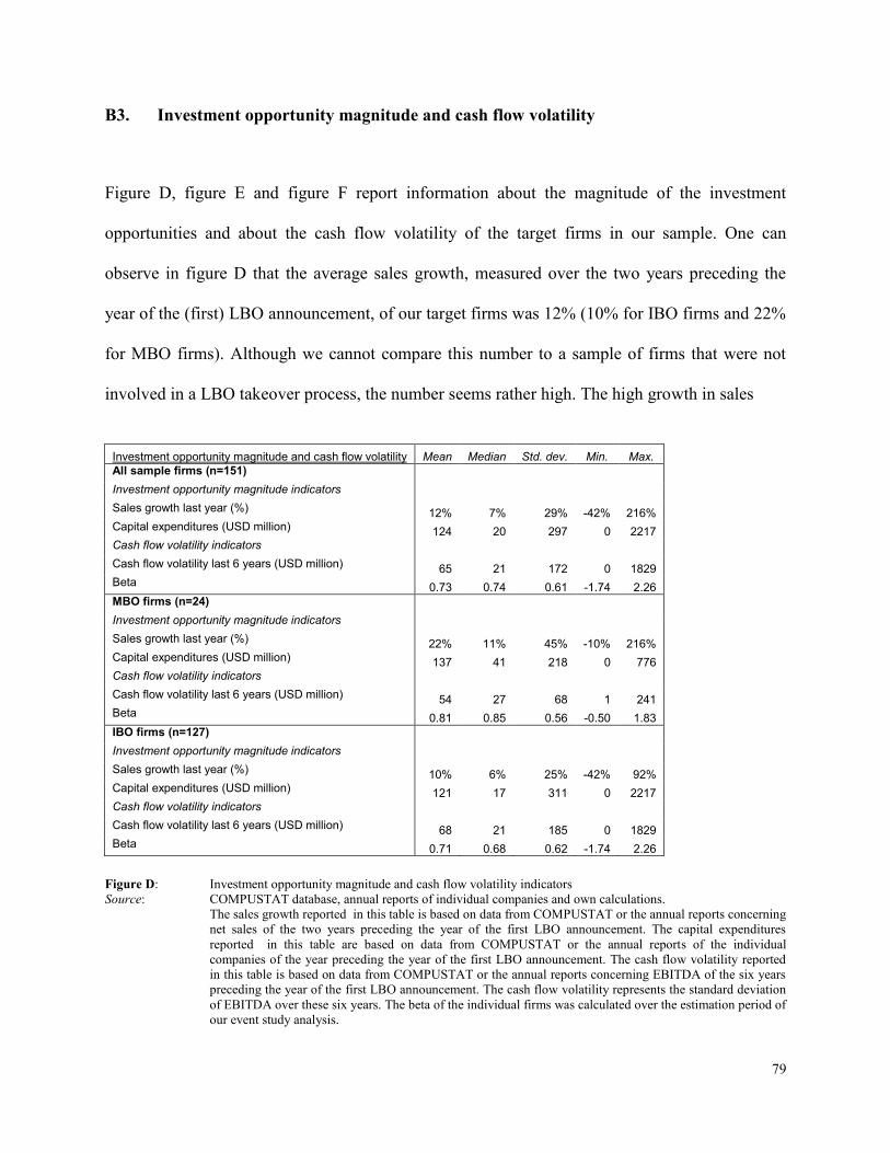
79

B3. Investment opportunity magnitude and cash flow volatility

Figure D, figure E and figure F report information about the magnitude of the investment

opportunities and about the cash flow volatility of the target firms in our sample. One can

observe in figure D that the average sales growth, measured over the two years preceding the

year of the (first) LBO announcement, of our target firms was 12% (10% for IBO firms and 22%

for MBO firms). Although we cannot compare this number to a sample of firms that were not

involved in a LBO takeover process, the number seems rather high. The high growth in sales

Investment opportunity magnitude and cash flow volatility Mean Median Std. dev. Min. Max.

All sample firms (n=151) Investment opportunity magnitude indicators

Sales growth last year (%) 12% 7% 29% -42% 216% Capital expenditures (USD million) 124 20 297 0 2217 Cash flow volatility indicators

Cash flow volatility last 6 years (USD million) 65 21 172 0 1829 Beta 0.73 0.74 0.61 -1.74 2.26

MBO firms (n=24) Investment opportunity magnitude indicators

Sales growth last year (%) 22% 11% 45% -10% 216% Capital expenditures (USD million) 137 41 218 0 776 Cash flow volatility indicators

Cash flow volatility last 6 years (USD million) 54 27 68 1 241 Beta 0.81 0.85 0.56 -0.50 1.83

IBO firms (n=127)

Investment opportunity magnitude indicators

Sales growth last year (%) 10% 6% 25% -42% 92% Capital expenditures (USD million) 121 17 311 0 2217 Cash flow volatility indicators

Cash flow volatility last 6 years (USD million) 68 21 185 0 1829 Beta 0.71 0.68 0.62 -1.74 2.26

Figure D: Investment opportunity magnitude and cash flow volatility indicators

Source: COMPUSTAT database, annual reports of individual companies and own calculations.

The sales growth reported in this table is based on data from COMPUSTAT or the annual reports concerning

net sales of the two years preceding the year of the first LBO announcement. The capital expenditures

reported in this table are based on data from COMPUSTAT or the annual reports of the individual

companies of the year preceding the year of the first LBO announcement. The cash flow volatility reported

in this table is based on data from COMPUSTAT or the annual reports concerning EBITDA of the six years

preceding the year of the first LBO announcement. The cash flow volatility represents the standard deviation

of EBITDA over these six years. The beta of the individual firms was calculated over the estimation period of

our event study analysis.

80

observed among the firms in our sample suggests high growth firms are more likely targets for

LBOs. In addition, figure D indicates average capital expenditures to be USD 124 million,

average cash flow volatility over the 6 years preceding the year of the (first) LBO announcement

to be USD 65 million and an average beta coefficient of 0.73. These numbers do not differ too

much between MBO and IBO firms. The average beta coefficient observed is lower than one,

which indicates the stock returns of our sample firms are less prone to swings in the business

cycle than the average firm. Among our sample firms we do observe firms with negative beta

coefficients, which indicates these firm‟s stock returns move opposite to the returns on the

market index. In total, only 11 firms in our sample have a negative beta coefficient.

Figure E shows how many firms in our sample spend money on research and development and

how many firms possess patents or trademarks. Figure F reports information concerning the

magnitude of R&D expenses and the number of patents for the firms that actually spend money

on R&D and that actually possess patents or trademarks. One can observe that 43 firms in our

sample have positive R&D expenses and 53 firms in our sample possess patents or trademarks.

Figure F shows that the average R&D expenses of our sample firms amount to USD 61 million

and that the average amount of patents or trademarks our sample firms possess amounts to 271.

These numbers are substantially lower for MBO firms than for IBO firms, which can be

explained by the fact that the MBO firms are of smaller size than the IBO firms. Consequently,

the MBO firms have less resources at their disposal than IBO firms to invest in R&D or patents.

The firms that have positive R&D expenses often do also possess patents or trademarks, which is

not surprising as patents and trademarks are only filed for when serious research and

development activity has taken place already. In total, 67 of the firms in our sample have positive

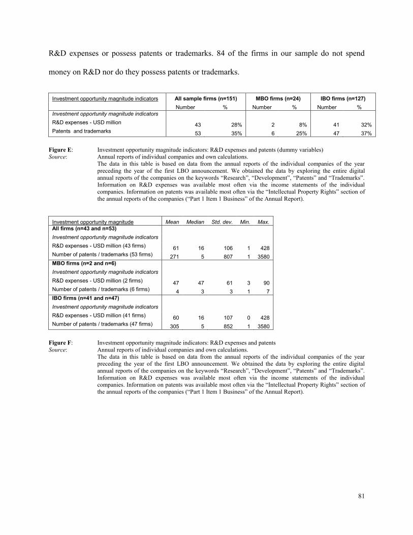
81

R&D expenses or possess patents or trademarks. 84 of the firms in our sample do not spend

money on R&D nor do they possess patents or trademarks.

Investment opportunity magnitude indicators All sample firms (n=151) MBO firms (n=24) IBO firms (n=127)

Number % Number % Number %

Investment opportunity magnitude indicators R&D expenses - USD million 43 28% 2 8% 41 32% Patents and trademarks 53 35% 6 25% 47 37%

Figure E: Investment opportunity magnitude indicators: R&D expenses and patents (dummy variables)

Source: Annual reports of individual companies and own calculations.

The data in this table is based on data from the annual reports of the individual companies of the year

preceding the year of the first LBO announcement. We obtained the data by exploring the entire digital

annual reports of the companies on the keywords “Research”, “Development”, “Patents” and “Trademarks”.

Information on R&D expenses was available most often via the income statements of the individual

companies. Information on patents was available most often via the “Intellectual Property Rights” section of

the annual reports of the companies (“Part 1 Item 1 Business” of the Annual Report).

Investment opportunity magnitude Mean Median Std. dev. Min. Max.

All firms (n=43 and n=53) Investment opportunity magnitude indicators

R&D expenses - USD million (43 firms) 61 16 106 1 428 Number of patents / trademarks (53 firms) 271 5 807 1 3580

MBO firms (n=2 and n=6) Investment opportunity magnitude indicators

R&D expenses - USD million (2 firms) 47 47 61 3 90 Number of patents / trademarks (6 firms) 4 3 3 1 7

IBO firms (n=41 and n=47) Investment opportunity magnitude indicators

R&D expenses - USD million (41 firms) 60 16 107 0 428 Number of patents / trademarks (47 firms) 305 5 852 1 3580

Figure F: Investment opportunity magnitude indicators: R&D expenses and patents

Source: Annual reports of individual companies and own calculations.

The data in this table is based on data from the annual reports of the individual companies of the year

preceding the year of the first LBO announcement. We obtained the data by exploring the entire digital

annual reports of the companies on the keywords “Research”, “Development”, “Patents” and “Trademarks”.

Information on R&D expenses was available most often via the income statements of the individual

companies. Information on patents was available most often via the “Intellectual Property Rights” section of

the annual reports of the companies (“Part 1 Item 1 Business” of the Annual Report).

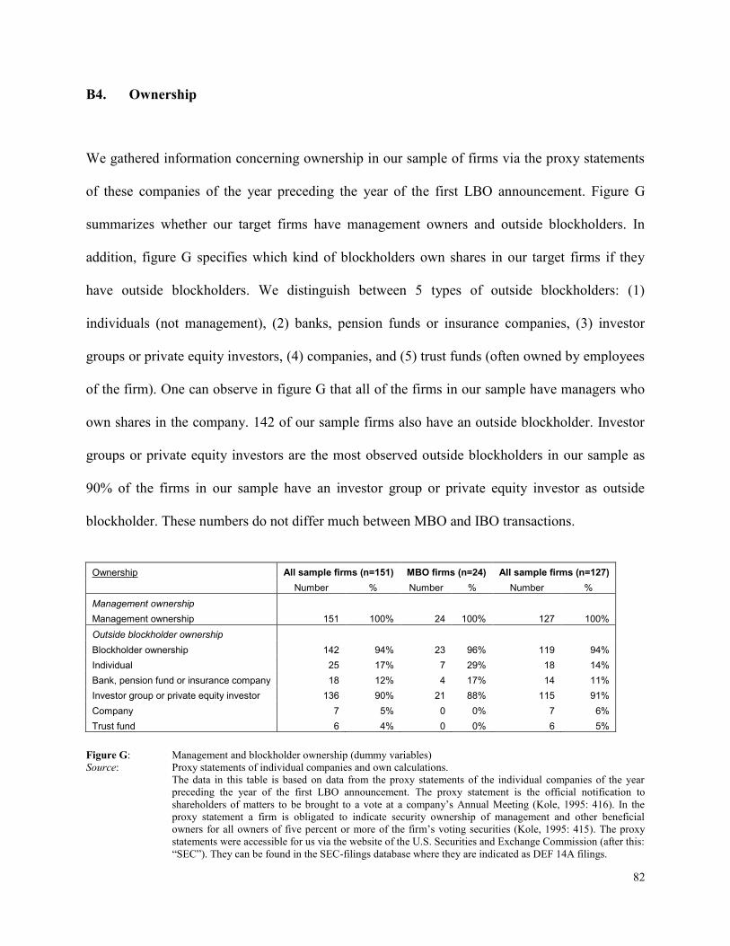
82

B4. Ownership

We gathered information concerning ownership in our sample of firms via the proxy statements

of these companies of the year preceding the year of the first LBO announcement. Figure G

summarizes whether our target firms have management owners and outside blockholders. In

addition, figure G specifies which kind of blockholders own shares in our target firms if they

have outside blockholders. We distinguish between 5 types of outside blockholders: (1)

individuals (not management), (2) banks, pension funds or insurance companies, (3) investor

groups or private equity investors, (4) companies, and (5) trust funds (often owned by employees

of the firm). One can observe in figure G that all of the firms in our sample have managers who

own shares in the company. 142 of our sample firms also have an outside blockholder. Investor

groups or private equity investors are the most observed outside blockholders in our sample as

90% of the firms in our sample have an investor group or private equity investor as outside

blockholder. These numbers do not differ much between MBO and IBO transactions.

Ownership All sample firms (n=151) MBO firms (n=24) All sample firms (n=127)

Number % Number % Number %

Management ownership

Management ownership 151 100% 24 100% 127 100%

Outside blockholder ownership

Blockholder ownership 142 94% 23 96% 119 94%

Individual 25 17% 7 29% 18 14%

Bank, pension fund or insurance company 18 12% 4 17% 14 11%

Investor group or private equity investor 136 90% 21 88% 115 91%

Company 7 5% 0 0% 7 6%

Trust fund 6 4% 0 0% 6 5%

Figure G: Management and blockholder ownership (dummy variables)

Source: Proxy statements of individual companies and own calculations.

The data in this table is based on data from the proxy statements of the individual companies of the year

preceding the year of the first LBO announcement. The proxy statement is the official notification to

shareholders of matters to be brought to a vote at a company‟s Annual Meeting (Kole, 1995: 416). In the

proxy statement a firm is obligated to indicate security ownership of management and other beneficial

owners for all owners of five percent or more of the firm‟s voting securities (Kole, 1995: 415). The proxy

statements were accessible for us via the website of the U.S. Securities and Exchange Commission (after this:

“SEC”). They can be found in the SEC-filings database where they are indicated as DEF 14A filings.

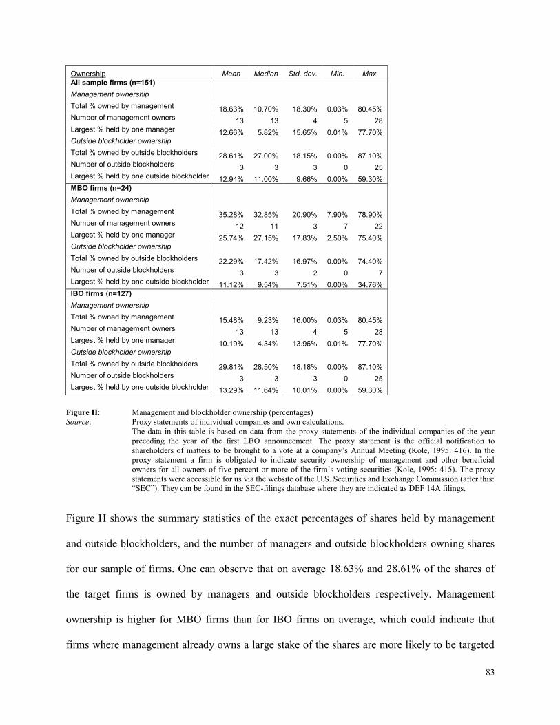
83

Ownership Mean Median Std. dev. Min. Max.

All sample firms (n=151) Management ownership

Total % owned by management 18.63% 10.70% 18.30% 0.03% 80.45% Number of management owners 13 13 4 5 28 Largest % held by one manager 12.66% 5.82% 15.65% 0.01% 77.70% Outside blockholder ownership

Total % owned by outside blockholders 28.61% 27.00% 18.15% 0.00% 87.10% Number of outside blockholders 3 3 3 0 25 Largest % held by one outside blockholder 12.94% 11.00% 9.66% 0.00% 59.30%

MBO firms (n=24) Management ownership

Total % owned by management 35.28% 32.85% 20.90% 7.90% 78.90% Number of management owners 12 11 3 7 22 Largest % held by one manager 25.74% 27.15% 17.83% 2.50% 75.40% Outside blockholder ownership

Total % owned by outside blockholders 22.29% 17.42% 16.97% 0.00% 74.40% Number of outside blockholders 3 3 2 0 7 Largest % held by one outside blockholder 11.12% 9.54% 7.51% 0.00% 34.76%

IBO firms (n=127)

Management ownership

Total % owned by management 15.48% 9.23% 16.00% 0.03% 80.45% Number of management owners 13 13 4 5 28 Largest % held by one manager 10.19% 4.34% 13.96% 0.01% 77.70% Outside blockholder ownership

Total % owned by outside blockholders 29.81% 28.50% 18.18% 0.00% 87.10% Number of outside blockholders 3 3 3 0 25 Largest % held by one outside blockholder 13.29% 11.64% 10.01% 0.00% 59.30%

Figure H: Management and blockholder ownership (percentages)

Source: Proxy statements of individual companies and own calculations.

The data in this table is based on data from the proxy statements of the individual companies of the year

preceding the year of the first LBO announcement. The proxy statement is the official notification to

shareholders of matters to be brought to a vote at a company‟s Annual Meeting (Kole, 1995: 416). In the

proxy statement a firm is obligated to indicate security ownership of management and other beneficial

owners for all owners of five percent or more of the firm‟s voting securities (Kole, 1995: 415). The proxy

statements were accessible for us via the website of the U.S. Securities and Exchange Commission (after this:

“SEC”). They can be found in the SEC-filings database where they are indicated as DEF 14A filings.

Figure H shows the summary statistics of the exact percentages of shares held by management

and outside blockholders, and the number of managers and outside blockholders owning shares

for our sample of firms. One can observe that on average 18.63% and 28.61% of the shares of

the target firms is owned by managers and outside blockholders respectively. Management

ownership is higher for MBO firms than for IBO firms on average, which could indicate that

firms where management already owns a large stake of the shares are more likely to be targeted

84

for MBOs. On the other hand, average blockholder ownership is higher for IBO firms than for

MBO firms. On average our sample firms have 13 management owners and 3 outside

blockholders. These numbers do not differ much between MBO and IBO transactions.

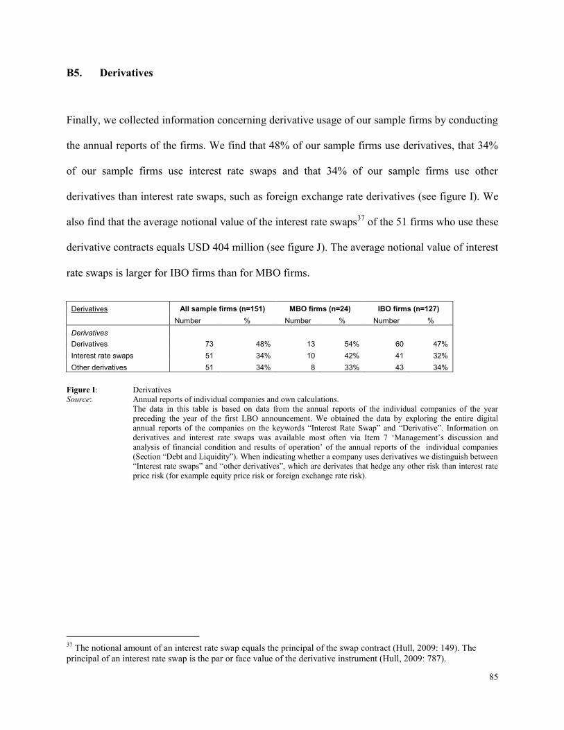
85

B5. Derivatives

Finally, we collected information concerning derivative usage of our sample firms by conducting

the annual reports of the firms. We find that 48% of our sample firms use derivatives, that 34%

of our sample firms use interest rate swaps and that 34% of our sample firms use other

derivatives than interest rate swaps, such as foreign exchange rate derivatives (see figure I). We

also find that the average notional value of the interest rate swaps37

of the 51 firms who use these

derivative contracts equals USD 404 million (see figure J). The average notional value of interest

rate swaps is larger for IBO firms than for MBO firms.

Derivatives All sample firms (n=151) MBO firms (n=24) IBO firms (n=127)

Number % Number % Number %

Derivatives

Derivatives 73 48% 13 54% 60 47%

Interest rate swaps 51 34% 10 42% 41 32%

Other derivatives 51 34% 8 33% 43 34%

Figure I: Derivatives

Source: Annual reports of individual companies and own calculations.

The data in this table is based on data from the annual reports of the individual companies of the year

preceding the year of the first LBO announcement. We obtained the data by exploring the entire digital

annual reports of the companies on the keywords “Interest Rate Swap” and “Derivative”. Information on

derivatives and interest rate swaps was available most often via Item 7 „Management‟s discussion and

analysis of financial condition and results of operation‟ of the annual reports of the individual companies

(Section “Debt and Liquidity”). When indicating whether a company uses derivatives we distinguish between

“Interest rate swaps” and “other derivatives”, which are derivates that hedge any other risk than interest rate

price risk (for example equity price risk or foreign exchange rate risk).

37

The notional amount of an interest rate swap equals the principal of the swap contract (Hull, 2009: 149). The

principal of an interest rate swap is the par or face value of the derivative instrument (Hull, 2009: 787).

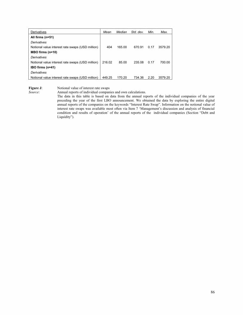
86

Derivatives Mean Median Std. dev. Min. Max.

All firms (n=51)

Derivatives

Notional value interest rate swaps (USD million) 404 165.00 670.91 0.17 3579.20

MBO firms (n=10)

Derivatives

Notional value interest rate swaps (USD million) 216.02 85.00 235.08 0.17 700.00

IBO firms (n=41)

Derivatives

Notional value interest rate swaps (USD million) 449.25 170.20 734.36 2.20 3579.20

Figure J: Notional value of interest rate swaps

Source: Annual reports of individual companies and own calculations.

The data in this table is based on data from the annual reports of the individual companies of the year

preceding the year of the first LBO announcement. We obtained the data by exploring the entire digital

annual reports of the companies on the keywords “Interest Rate Swap”. Information on the notional value of

interest rate swaps was available most often via Item 7 „Management‟s discussion and analysis of financial

condition and results of operation‟ of the annual reports of the individual companies (Section “Debt and

Liquidity”).

87

B6. Summary

The descriptive statistics show that most of the LBO announcements of the target firms in our

sample were made in 2007, which is very likely to be caused by the credit crisis. It also shows

that 52% of the proposed transactions we investigate are characterized by a proposed transaction

value of more than USD 500 million. The average size of the firms considered in our sample

seems quite large in relation to other studies that investigate the abnormal returns of LBO

announcements. According to Renneboog, Simons and Wright (2007: 601) it is more likely that

larger firms are targeted by institutional buyers who possess over specialized financial

engineering capabilities instead of management teams. Consequently, it is not illogical we find

so many IBO target firms in our sample. Sales growth also seems to be high for our sample

firms, which could suggest high growth firms are more likely targets for LBOs. The average

return on assets, however, of the firms in our sample is -2%, which can probably be partly

explained by the effect of the credit crisis on the accounting performance of our firms and by the

notion that LBO firms are likely to be firms that underperform the market. The average beta

coefficient observed for our sample firms is lower than one, which indicates the stock returns of

our sample firms are less prone to swings in the business cycle than the average firm. In total,

44% of the firms we consider has R&D expenses or possesses patents or trademarks. Finally, all

sample firms have management owners, almost all sample firms have blockholder owners and

48% of the sample firms uses derivatives.

We can conclude on the basis of the descriptive statistics that the target firms of our sample are

not drawn from a homogeneous population. The announcements of MBO deals are more often

88

announcements of deals that are eventually not completed than the announcements of IBO deals.

This could suggest the closing probability of MBO deals is lower than that of IBO deals. In

addition, the MBO target firms are on average of smaller size than the IBO target firms, which

underwrites the idea of Renneboog, Simons and Wright (2007: 601) that larger firms are more

likely to be targeted by institutional buyers who possess over specialized financial engineering

capabilities than by management teams. IBO target firms have higher R&D expenditures and

more patents than MBO target firms, which can probably be explained by the larger size and

consequently the larger magnitude of resources of these companies. The MBO target firms are

also characterized by a higher return on assets ratio than IBO target firms, which seem to suggest

MBO target firms are more likely to be better performing firms than IBO firms. The higher sales

growth observed for MBO target firms in relation to IBO firms seems to confirm this idea.

Finally, while management ownership is higher for MBO target firms than for IBO target firms,

blockholder ownership is higher for IBO target firms than for MBO target firms. The fact that

management ownership is higher for the MBO target firms could indicate that firms where

management already owns a large stake of the shares are more likely to be targeted for MBOs.

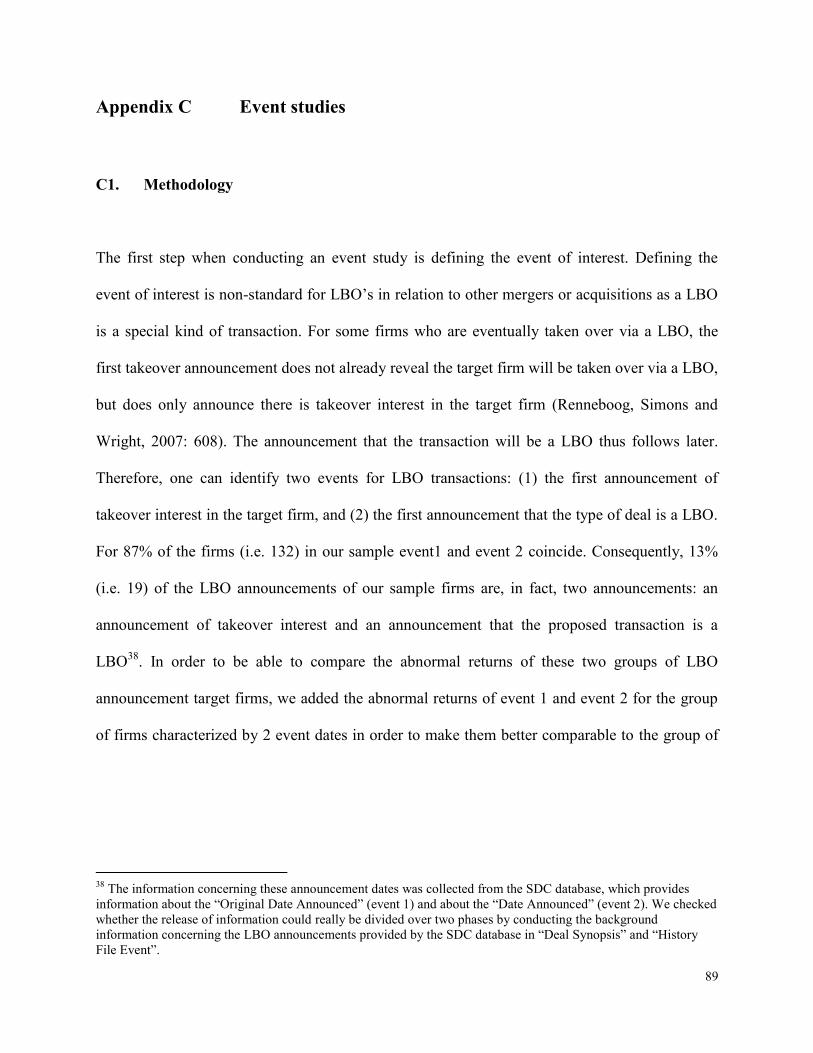
89

Appendix C Event studies

C1. Methodology

The first step when conducting an event study is defining the event of interest. Defining the

event of interest is non-standard for LBO‟s in relation to other mergers or acquisitions as a LBO

is a special kind of transaction. For some firms who are eventually taken over via a LBO, the

first takeover announcement does not already reveal the target firm will be taken over via a LBO,

but does only announce there is takeover interest in the target firm (Renneboog, Simons and

Wright, 2007: 608). The announcement that the transaction will be a LBO thus follows later.

Therefore, one can identify two events for LBO transactions: (1) the first announcement of

takeover interest in the target firm, and (2) the first announcement that the type of deal is a LBO.

For 87% of the firms (i.e. 132) in our sample event1 and event 2 coincide. Consequently, 13%

(i.e. 19) of the LBO announcements of our sample firms are, in fact, two announcements: an

announcement of takeover interest and an announcement that the proposed transaction is a

LBO38

. In order to be able to compare the abnormal returns of these two groups of LBO

announcement target firms, we added the abnormal returns of event 1 and event 2 for the group

of firms characterized by 2 event dates in order to make them better comparable to the group of

38

The information concerning these announcement dates was collected from the SDC database, which provides

information about the “Original Date Announced” (event 1) and about the “Date Announced” (event 2). We checked

whether the release of information could really be divided over two phases by conducting the background

information concerning the LBO announcements provided by the SDC database in “Deal Synopsis” and “History

File Event”.

90

firms characterized by 1 event date39

. Naturally, we excluded overlap in the event windows of

event 1 and event 2 for the first group of firms.

Figure K: Estimation window and event windows for LBOs

Source: Jong, de F. (2009: 4)

The second step when conducting an event study is defining the event window, the period over

which the stock market returns on the securities of the firms examined are observed. In figure K

one can observe the time line around the event on the basis of which the methodology of event

studies can be made more visual. One can observe the two event windows in figure K for event 1

and for event 2. The precise event days are indicated by in the middle of the event

windows. The event windows run from till for event 1 [ ] and from till for

event 2 [ ]. The event window is often set broader than the specific period of interest, in

order to examine the periods close to the event. We examine five event windows: (1) one trading

day before the event to one trading day after the event [-1,+1], (2) five trading days before the

event to five trading days after the event [-5,+5], (3) twenty trading days before the event to

twenty trading days after the event [-20,+20], (4) forty trading days before the event to forty

39

In our sample there are 19 firms for which event 1 and event 2 do not coincide. For 5 of these firms event 1 and

event 2 take place on 2 successive days. For these firms we took the date of event 2 as . Since the event dates

are clustered so closely together for these firms we did not add the returns of the 2 event dates in order to determine

the abnormal return at , but assumed event 1 to be and event 2 to be . Since both dates fall under

the event window [ ], we feel the assumption can be well defended.

91

trading days after the event [-40,+40], and (5) sixty trading days before the event to sixty trading

days after the event [-60,+60].

The third step when conducting an event study is defining a measure of the abnormal return,

which is the actual return on a firm‟s stock during the event window minus the normal return on

a firm‟s stock during the event window: , where represents abnormal

return, represents actual return and represents normal return (MacKinlay, 1997: 15). We

calculate the daily actual returns by the following formula:

, where are the

unadjusted share prices of the companies‟ securities we gathered via Datastream40

. There are

several approaches to estimate the normal return on a firm‟s stock. In general these approaches

can be divided into two groups: (1) statistical approaches, and (2) economic approaches.

Statistical approaches construct normal returns by relying on statistical assumptions concerning

the behavior of asset returns. Economic approaches add assumptions on investor behavior to the

statistical assumptions and are therefore better able of calculating more precise measures of

normal return (MacKinlay, 1997: 15). Because of this preciseness we choose to use an economic

approach to measure normal returns, namely a CAPM type model: ( ),

where represents the risk free rate , where represents an OLS estimate of the beta

coefficient of a firms‟ security, where represents the market index return and where

( ) represents the market risk premium. We downloaded our market index proxy

40

Since the share prices gathered via Datastream contain share prices of dates which are actually no transaction days

(such as, for example, Christmas) and the data on the market index proxy (CRSP equally-weighted daily returns on

the S&P 500 index excluding dividends) we use does not contain these dates, we had to remove the non-transaction

dates (approximately 9 days a year) from the share price data provided by Datastream in order to make the data

comparable to the market index proxy return data.

92

(CRSP equally-weighted daily returns on the S&P 500 index excluding dividends) and the three-

month Treasury Bill rate from the CRSP database which was accessible for us via WRDS41

.

One needs to identify an estimation window to measure the of the CAPM type model in order

to be able to construct the measure of normal returns in the event window. In order to prevent

overlap and interdependencies the estimation window usually precedes the event window. The

estimation window is also shown on the time line depicted in figure K. The estimation window

runs from till [ ]. We use an estimation window that starts 317 trading days before

event 1 and that ends 66 trading days before event 1. Consequently, we use an estimation period

of 252 transaction days, which approximately covers one calendar year, for our event studies.

We estimate the beta coefficient of each stock over this estimation window by making use of the

market model ( ). Consequently, the beta coefficient we use to determine

normal returns is the OLS estimate of the regression coefficient of beta in the following

regression: 42. According to Bradfield (2003: 47) the market model has

traditionally been used to estimate the beta coefficient.

41

Since the data concerning the three-month Treasury Bill rate were daily quoted in terms of yearly rates and

defined as percentages we had to transform the data to daily rates and fractions conform the following formula:

[(

)

] . Because the market index return data were already daily quoted in terms of daily rates and

defined as fractions, we did not have to transform these data. 42

According to Bradley (2003: 47) the market model is usually estimated by running ordinary least square

regressions (after this: “OLS”). We run these regressions in Microsoft Excel. The OLS estimate of beta is equal to:

.

93

C2. Results

The abnormal returns of the LBO announcements for our sample of firms are depicted in figure

L. We show the abnormal returns as cumulative average abnormal returns (“CAARs”)43

. One

can observe that the CAAR over the event window [-1,+1] amounts to 22.94% for all our sample

firms and increases to 30.63% for the largest event window considered [-60,+60]. One can

observe in figure 2 depicted in paragraph 2.1 that these results are quite comparable to previous

empirical evidence on the CAARs of LBO announcements. The CAARs are also depicted

separately for the firms where event 1 and event 2 coincide (“1 event firms”) and for the firms

where event 1 and event 2 do not coincide (“2 event firms”). One can observe that the CAARs of

the 1 event firms are quite similar to the CAARs of the entire sample. The CAARs of the 2 event

firms differ more from the CAARs of the entire sample, i.e. they are considerably lower44

. We

test the null hypothesis that the CAARs are equal to zero with 2 parametric t-tests: (1) a simple t-

test used, among others, by Renneboog, Simons and Wright (2007: 622), which incorporates the

variance of event-induced abnormal returns, and (2) a t-test proposed by Kothari and Warner

(1997), in which the variance of the abnormal returns is determined in the estimation window. In

addition, we also run a non-parametric test: the generalized sign test proposed by Cowan (1992).

The results of the tests are also depicted in figure L. For the entire sample of firms the null

hypothesis can be rejected at a 1% significance level for the CAARs of all event windows on the

basis of all three test procedures. The same holds for the CAARs of the 1 event firms. The tests

of the CAARS of the 2 event firms are less conclusive, which is probably due to the low number

43

The specifications concerning the calculations of the CAARs are given in Appendix C3. 44

Because of the low number of observations of 2 event firms in our sample one cannot interpret these numbers as

representative for the CAARs of LBO announcements that come in two stages.

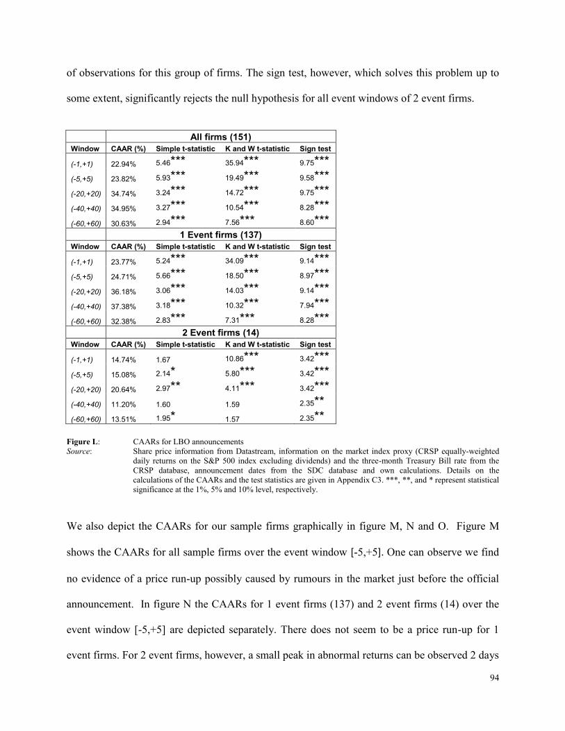
94

of observations for this group of firms. The sign test, however, which solves this problem up to

some extent, significantly rejects the null hypothesis for all event windows of 2 event firms.

All firms (151)

Window CAAR (%) Simple t-statistic K and W t-statistic Sign test

(-1,+1) 22.94% 5.46*** 35.94*** 9.75***

(-5,+5) 23.82% 5.93*** 19.49*** 9.58***

(-20,+20) 34.74% 3.24*** 14.72*** 9.75***

(-40,+40) 34.95% 3.27*** 10.54*** 8.28***

(-60,+60) 30.63% 2.94*** 7.56*** 8.60***

1 Event firms (137)

Window CAAR (%) Simple t-statistic K and W t-statistic Sign test

(-1,+1) 23.77% 5.24*** 34.09*** 9.14***

(-5,+5) 24.71% 5.66*** 18.50*** 8.97***

(-20,+20) 36.18% 3.06*** 14.03*** 9.14***

(-40,+40) 37.38% 3.18*** 10.32*** 7.94***

(-60,+60) 32.38% 2.83*** 7.31*** 8.28***

2 Event firms (14)

Window CAAR (%) Simple t-statistic K and W t-statistic Sign test

(-1,+1) 14.74% 1.67 10.86*** 3.42***

(-5,+5) 15.08% 2.14* 5.80*** 3.42***

(-20,+20) 20.64% 2.97** 4.11*** 3.42***

(-40,+40) 11.20% 1.60 1.59 2.35**

(-60,+60) 13.51% 1.95* 1.57 2.35**

Figure L: CAARs for LBO announcements

Source: Share price information from Datastream, information on the market index proxy (CRSP equally-weighted

daily returns on the S&P 500 index excluding dividends) and the three-month Treasury Bill rate from the

CRSP database, announcement dates from the SDC database and own calculations. Details on the

calculations of the CAARs and the test statistics are given in Appendix C3. ***, **, and * represent statistical

significance at the 1%, 5% and 10% level, respectively.

We also depict the CAARs for our sample firms graphically in figure M, N and O. Figure M

shows the CAARs for all sample firms over the event window [-5,+5]. One can observe we find

no evidence of a price run-up possibly caused by rumours in the market just before the official

announcement. In figure N the CAARs for 1 event firms (137) and 2 event firms (14) over the

event window [-5,+5] are depicted separately. There does not seem to be a price run-up for 1

event firms. For 2 event firms, however, a small peak in abnormal returns can be observed 2 days

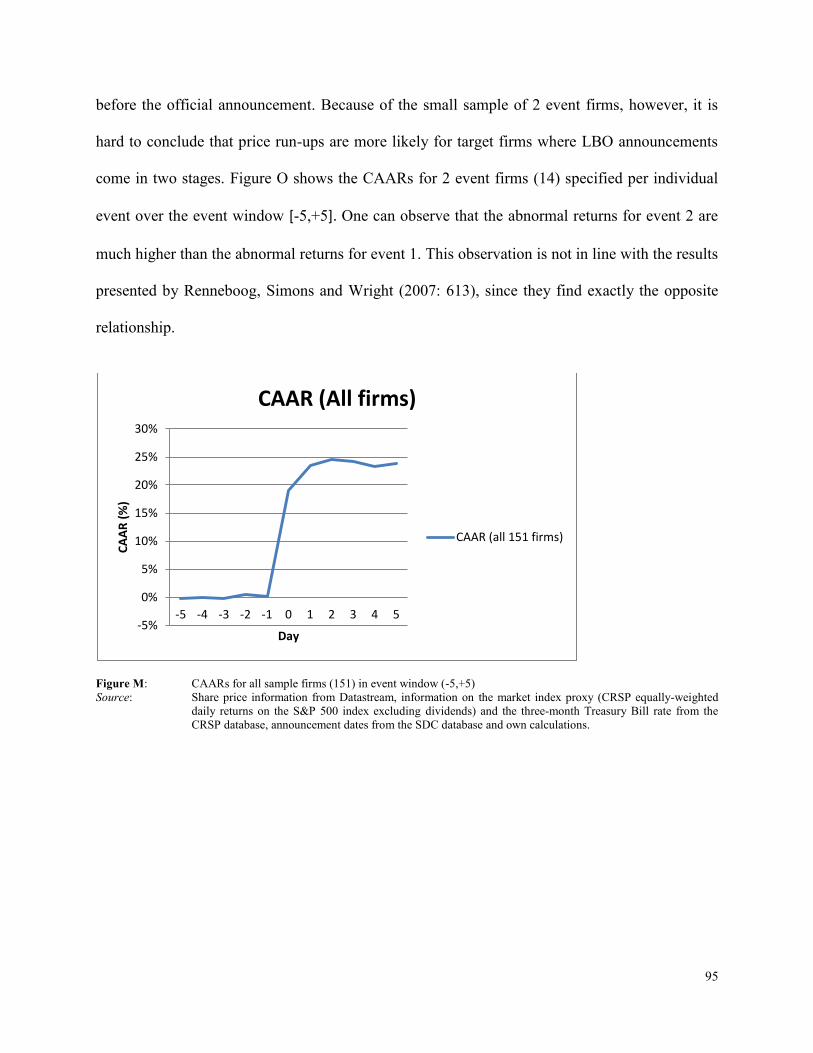
95

before the official announcement. Because of the small sample of 2 event firms, however, it is

hard to conclude that price run-ups are more likely for target firms where LBO announcements

come in two stages. Figure O shows the CAARs for 2 event firms (14) specified per individual

event over the event window [-5,+5]. One can observe that the abnormal returns for event 2 are

much higher than the abnormal returns for event 1. This observation is not in line with the results

presented by Renneboog, Simons and Wright (2007: 613), since they find exactly the opposite

relationship.

Figure M: CAARs for all sample firms (151) in event window (-5,+5)

Source: Share price information from Datastream, information on the market index proxy (CRSP equally-weighted

daily returns on the S&P 500 index excluding dividends) and the three-month Treasury Bill rate from the

CRSP database, announcement dates from the SDC database and own calculations.

-5%

0%

5%

10%

15%

20%

25%

30%

-5 -4 -3 -2 -1 0 1 2 3 4 5

CA

AR

(%

)

Day

CAAR (All firms)

CAAR (all 151 firms)

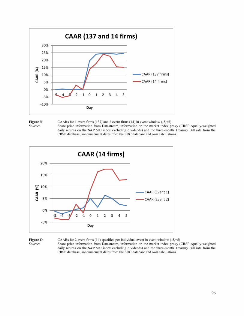
96

Figure N: CAARs for 1 event firms (137) and 2 event firms (14) in event window (-5,+5)

Source: Share price information from Datastream, information on the market index proxy (CRSP equally-weighted

daily returns on the S&P 500 index excluding dividends) and the three-month Treasury Bill rate from the

CRSP database, announcement dates from the SDC database and own calculations.

Figure O: CAARs for 2 event firms (14) specified per individual event in event window (-5,+5)

Source: Share price information from Datastream, information on the market index proxy (CRSP equally-weighted

daily returns on the S&P 500 index excluding dividends) and the three-month Treasury Bill rate from the

CRSP database, announcement dates from the SDC database and own calculations.

-10%

-5%

0%

5%

10%

15%

20%

25%

30%

-5 -4 -3 -2 -1 0 1 2 3 4 5

CA

AR

(%

)

Day

CAAR (137 and 14 firms)

CAAR (137 firms)

CAAR (14 firms)

-5%

0%

5%

10%

15%

20%

-5 -4 -3 -2 -1 0 1 2 3 4 5

CA

AR

(%

)

Day

CAAR (14 firms)

CAAR (Event 1)

CAAR (Event 2)

97

C3. Test statistics

When analyzing the abnormal returns of our sample firms we first group the abnormal returns

according to the matrix depicted in figure P.

Figure P: Matrix of abnormal returns

Source: Jong, de (2007: 7)

We define Average Abnormal Returns (AAR) of a specific transaction day by equation (1):

∑

where j represents the target firm and t represents a specific trading day.

98

We define Cumulative Abnormal Returns (CAR) over a specific time period for a specific target

firm by equation (2):

∑

where and represent the first and the final day of the event window.

We define Cumulative Average Abnormal Returns (CAAR) over a specific time period by

equation (3):

∑

Simple t-test (Renneboog, Simons and Wright, 2007: 622)

To test the null hypothesis that the CAARs are equal to zero we first use a simple t-test proposed,

among others, by Renneboog, Simons and Wright (2007: 622). According to Renneboog, Simons

and Wright (2007: 622) this test incorporates the variance of event-induced abnormal returns.

We incorporate this test as it is well possible that variance of the abnormal returns is different for

event and non-event periods. When the variance would, for example, increase in event periods,

the variances calculated for non-event periods would underestimate the real variance.

The test statistic can be computed by equation (4):

√ ⁄

Where N represents the number of target firms and is given by equation (5):

99

√

∑( )

Test statistic proposed by Kothari and Warner (1997)

Kothari and Warner (1997) calculate the variance of the abnormal returns in the estimation

window. Estimating the variance of the abnormal returns is primarily done to deal with the

problem of cross-sectional dependence (Jong, de, 2007: 13). Cross-sectional dependence means

that the abnormal returns of two different events are correlated: ( ) where

. Cross-sectional correlation between abnormal returns in our sample is well possible as

there is event clustering in our sample, i.e. the occurrence of more events in one period. To deal

with cross-sectional dependence we incorporate the crude dependence adjustment (Jong, de,

2007: 13) proposed, among others, by Kothari and Warner (1997) and Brown and Warner

(1980).

The test statistic can be computed by equation (6):

√

where represents the number of days in the event window and where is given by

equation (7):

√

∑

100

where and represent the first and the final day of the estimation window and where is

given by equation (8):

∑

Where T represents the number of transaction days in the estimation window.

Non-parametric generalized sign test (Cowan, 1992)

We also incorporate a non-parametric test to test the null hypothesis to resolve the problem that

the abnormal returns in our sample might have fat tails. The fat tails might be caused by the fact

we use daily data on stock returns, which are usually fat-tailed (Jong, de, 2007: 15). In addition,

the cross-section we have of 2 event firms is very small (14 firms), which may also lead to fat

tails. Consequently, we also use the non-parametric test to resolve this particular problem. In

general, one can use two non-parametric tests for event studies: (1) the sign test, and (2) the rank

test (Jong, de, 2007: 16-17). According to Cowan (1992: 23) the rank test provides more power

than the sign test. The power of the rank test, however, drops when the days in the event window

increase, when the sample contains thinly traded stocks and when the return variance increases

on the event date (Cowan, 1992: 23-24). Since we incorporate quite large event windows (121

days), since the securities we consider might be thinly traded and since the return variance might

indeed increase on the event date for our sample firms, we choose to use the generalized sign test

proposed by Cowan (1992).

101

We first define in equation (9):

∑

∑

where N represents the number of firms, where and represent the first and the final day of

the estimation window, where T represents the number of transaction days in the estimation

window and where is given by equation (10):

{

The test statistic is defined in equation (11):

[ ]

where w is defined as the number of positive CAARs in the event window.

102

Appendix D Regression analysis

D1. Test for heteroskedasticity

According to Wooldridge (2006: 56-57) heteroskedasticity means that the variance of the

unobservable error variable is not constant. Consequently, under heteroskedasticity the

assumption of homoskedasticity is violated. Under heteroskedasticty the “standard” formulas and

estimators of coefficients under ordinary least squares regression are invalid (Wooldridge, 2006:

60). Hence, we test our main regression for heteroskedasticity to make sure the assumption of

homoskedasticity holds and our coefficient estimates are not biased.

We test for heteroskedasticity by means of the White test (White, 1980). We execute this test

after running our regression in STATA by entering the command: estat imtest, white. Figure Q

shows the results of running the White test on our regression in STATA. As the p-value is quite

large, we cannot reject the null hypothesis of homoskedasticity.

White's test for Ho: Homoskedasticity

Against Ha: Unrestricted heteroskedasticity

Results

Chi2(150) 151

Prob > chi2 0.4617

Figure Q: White test for heteroskedasticity

Source: The regression was computed by conducting all data gathered for this study (see chapter 3). The

White test was executed using the statistical software program STATA.

103

D2. Tests for multicollinearity

According to Wooldridge (2006: 102) multicollinearity represents high (but not perfect)

correlation between two or more independent variables of a regression. The main problem of

multicollinearity is that the coefficient estimators of ordinary least squares regression exhibit

large variances, which may result in too large estimates and in signs that disagree with the

known theoretical properties of the variables (Mansfield and Helms, 1982: 159). In order to test

whether our main regression suffers from multicollinearity we performs 3 checks: (1) the

correlation matrix, (2) variance inflation factors and (3) the condition number.

Correlation matrix

According to Mansfield and Helms (1982: 158) one can detect multicollinearity by examining

the pairwise correlations between the independent variables of a regression. We examine these

correlations by conducting the correlation matrix of all our independent variables (see figure R).

We conducted the matrix in STATA by entering the command: pwcorr, independent variables,

sig. Although it is hard to determine when a correlation coefficient between two independent

variables is too high, we conclude that of the independent variables we use for our main

regression only three exhibit high correlation. The correlation coefficient between „Total Sales‟

and „Log Standard Deviation EBITDA‟ is 0.68 and significant at the 1% level. The correlation

coefficient between „Total Sales‟ and „EBIT‟ is 0.81 and significant at the 1% level. Although

these correlations are high, we do not feel the coefficients are that high we have to exclude the

variables from our regression. Excluding these variables, namely, would decrease the

explanatory power of our regression.

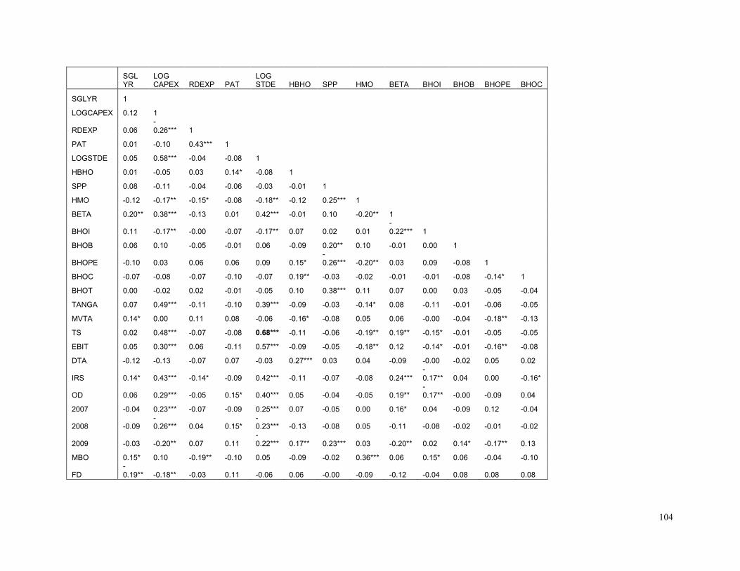
104

SGL YR

LOG CAPEX RDEXP PAT

LOG STDE HBHO SPP HMO BETA BHOI BHOB BHOPE BHOC

SGLYR 1

LOGCAPEX 0.12 1

RDEXP 0.06 -0.26*** 1

PAT 0.01 -0.10 0.43*** 1

LOGSTDE 0.05 0.58*** -0.04 -0.08 1

HBHO 0.01 -0.05 0.03 0.14* -0.08 1

SPP 0.08 -0.11 -0.04 -0.06 -0.03 -0.01 1

HMO -0.12 -0.17** -0.15* -0.08 -0.18** -0.12 0.25*** 1

BETA 0.20** 0.38*** -0.13 0.01 0.42*** -0.01 0.10 -0.20** 1

BHOI 0.11 -0.17** -0.00 -0.07 -0.17** 0.07 0.02 0.01 -0.22*** 1

BHOB 0.06 0.10 -0.05 -0.01 0.06 -0.09 0.20** 0.10 -0.01 0.00 1

BHOPE -0.10 0.03 0.06 0.06 0.09 0.15* -0.26*** -0.20** 0.03 0.09 -0.08 1

BHOC -0.07 -0.08 -0.07 -0.10 -0.07 0.19** -0.03 -0.02 -0.01 -0.01 -0.08 -0.14* 1

BHOT 0.00 -0.02 0.02 -0.01 -0.05 0.10 0.38*** 0.11 0.07 0.00 0.03 -0.05 -0.04

TANGA 0.07 0.49*** -0.11 -0.10 0.39*** -0.09 -0.03 -0.14* 0.08 -0.11 -0.01 -0.06 -0.05

MVTA 0.14* 0.00 0.11 0.08 -0.06 -0.16* -0.08 0.05 0.06 -0.00 -0.04 -0.18** -0.13

TS 0.02 0.48*** -0.07 -0.08 0.68*** -0.11 -0.06 -0.19** 0.19** -0.15* -0.01 -0.05 -0.05

EBIT 0.05 0.30*** 0.06 -0.11 0.57*** -0.09 -0.05 -0.18** 0.12 -0.14* -0.01 -0.16** -0.08

DTA -0.12 -0.13 -0.07 0.07 -0.03 0.27*** 0.03 0.04 -0.09 -0.00 -0.02 0.05 0.02

IRS 0.14* 0.43*** -0.14* -0.09 0.42*** -0.11 -0.07 -0.08 0.24*** -0.17** 0.04 0.00 -0.16*

OD 0.06 0.29*** -0.05 0.15* 0.40*** 0.05 -0.04 -0.05 0.19** -0.17** -0.00 -0.09 0.04

2007 -0.04 0.23*** -0.07 -0.09 0.25*** 0.07 -0.05 0.00 0.16* 0.04 -0.09 0.12 -0.04

2008 -0.09 -0.26*** 0.04 0.15*

-0.23*** -0.13 -0.08 0.05 -0.11 -0.08 -0.02 -0.01 -0.02

2009 -0.03 -0.20** 0.07 0.11 -0.22*** 0.17** 0.23*** 0.03 -0.20** 0.02 0.14* -0.17** 0.13

MBO 0.15* 0.10 -0.19** -0.10 0.05 -0.09 -0.02 0.36*** 0.06 0.15* 0.06 -0.04 -0.10

FD -0.19** -0.18** -0.03 0.11 -0.06 0.06 -0.00 -0.09 -0.12 -0.04 0.08 0.08 0.08

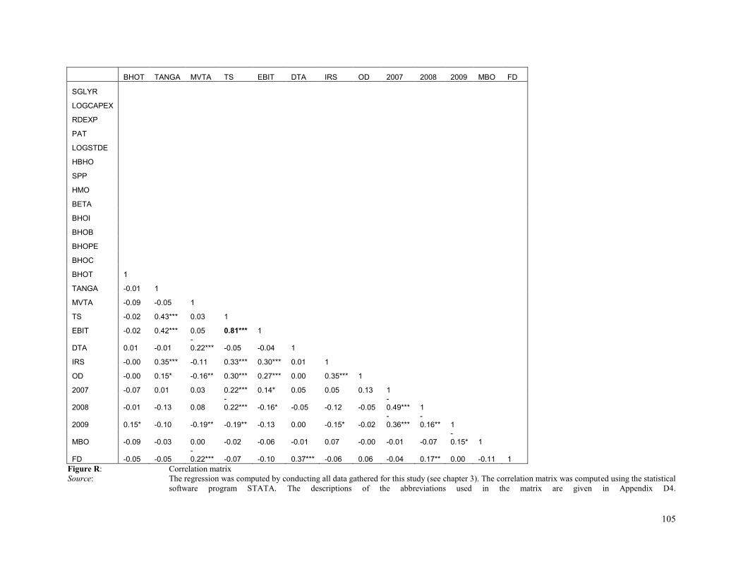
105

BHOT TANGA MVTA TS EBIT DTA IRS OD 2007 2008 2009 MBO FD

SGLYR

LOGCAPEX

RDEXP

PAT

LOGSTDE

HBHO

SPP

HMO

BETA

BHOI

BHOB

BHOPE

BHOC

BHOT 1

TANGA -0.01 1

MVTA -0.09 -0.05 1

TS -0.02 0.43*** 0.03 1

EBIT -0.02 0.42*** 0.05 0.81*** 1

DTA 0.01 -0.01 -0.22*** -0.05 -0.04 1

IRS -0.00 0.35*** -0.11 0.33*** 0.30*** 0.01 1

OD -0.00 0.15* -0.16** 0.30*** 0.27*** 0.00 0.35*** 1

2007 -0.07 0.01 0.03 0.22*** 0.14* 0.05 0.05 0.13 1

2008 -0.01 -0.13 0.08 -0.22*** -0.16* -0.05 -0.12 -0.05

-0.49*** 1

2009 0.15* -0.10 -0.19** -0.19** -0.13 0.00 -0.15* -0.02 -0.36***

-0.16** 1

MBO -0.09 -0.03 0.00 -0.02 -0.06 -0.01 0.07 -0.00 -0.01 -0.07 -0.15* 1

FD -0.05 -0.05 -0.22*** -0.07 -0.10 0.37*** -0.06 0.06 -0.04 0.17** 0.00 -0.11 1

Figure R: Correlation matrix

Source: The regression was computed by conducting all data gathered for this study (see chapter 3). The correlation matrix was computed using the statistical

software program STATA. The descriptions of the abbreviations used in the matrix are given in Appendix D4.

106

Variance inflation factors

Variable VIF 1/VIF

TS 4.26 0.23

EBIT 3.75 0.27

LOGSTDE 2.98 0.34

LOGCAPEX 2.53 0.40

2007 2.08 0.48

2008 2.01 0.50

2009 1.89 0.53

BETA 1.67 0.60

HMO 1.65 0.61

TANGA 1.63 0.61

RDEXP 1.61 0.62

SPP 1.55 0.65

IRS 1.54 0.65

PAT 1.53 0.65

OD 1.5 0.67

MBO 1.47 0.68

BHOPE 1.46 0.68

FD 1.39 0.72

DT 1.36 0.74

MVTA 1.36 0.74

HBHO 1.34 0.75

BHOT 1.26 0.80

SGLYR 1.25 0.80

BHOC 1.23 0.82

BHOI 1.22 0.82

BHOB 1.15 0.87

Mean VIF 1.79

Figure S: VIFs of independent variables

Source: The regression was computed by

conducting all data gathered for this

study (see chapter 3). The VIFs were

computed using the statistical software

program STATA. The descriptions of

the abbreviations are given in Appendix

D4.

According to Mansfield and Helms (1982: 158)

multicollinearity can also be detected by

examining the variance inflation factors of the

independent variables (VIF). We compute the

VIFs in STATA by entering the command vif

after running our regression. The results are

presented in figure S. Horimoto and Toh (2000:

248) indicate that a popular cutoff value of VIF

is 10. Consequently, when the VIF of an

independent variable is larger than 10, the

variable shows multicollinearity (Horimoto and

Toh, 2000: 248). We can conclude that no

independent variable used in our regression has

a VIF larger than 10.

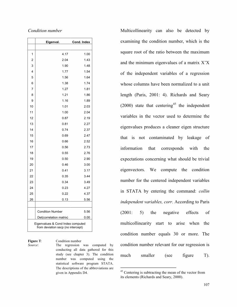
107

Condition number

Eigenval. Cond. Index

1 4.17 1.00

2 2.04 1.43

3 1.90 1.48

4 1.77 1.54

5 1.56 1.64

6 1.38 1.74

7 1.27 1.81

8 1.21 1.86

9 1.16 1.89

10 1.01 2.03

11 1.00 2.04

12 0.87 2.19

13 0.81 2.27

14 0.74 2.37

15 0.69 2.47

16 0.66 2.52

17 0.56 2.73

18 0.55 2.76

19 0.50 2.90

20 0.46 3.00

21 0.41 3.17

22 0.35 3.44

23 0.34 3.49

24 0.23 4.27

25 0.22 4.37

26 0.13 5.56

Condition Number 5.56

Det(correlation matrix) 0.00

Eigenvalues & Cond Index computed from deviation sscp (no intercept)

Figure T: Condition number

Source: The regression was computed by

conducting all data gathered for this

study (see chapter 3). The condition

number was computed using the

statistical software program STATA.

The descriptions of the abbreviations are

given in Appendix D4.

Multicollinearity can also be detected by

examining the condition number, which is the

square root of the ratio between the maximum

and the minimum eigenvalues of a matrix X‟X

of the independent variables of a regression

whose columns have been normalized to a unit

length (Paris, 2001: 4). Richards and Seary

(2000) state that centering45

the independent

variables in the vector used to determine the

eigenvalues produces a cleaner eigen structure

that is not contaminated by leakage of

information that corresponds with the

expectations concerning what should be trivial

eigenvectors. We compute the condition

number for the centered independent variables

in STATA by entering the command: collin

independent variables, corr. According to Paris

(2001: 5) the negative effects of

multicollinearity start to arise when the

condition number equals 30 or more. The

condition number relevant for our regression is

much smaller (see figure T).

45

Centering is subtracting the mean of the vector from

its elements (Richards and Seary, 2000).

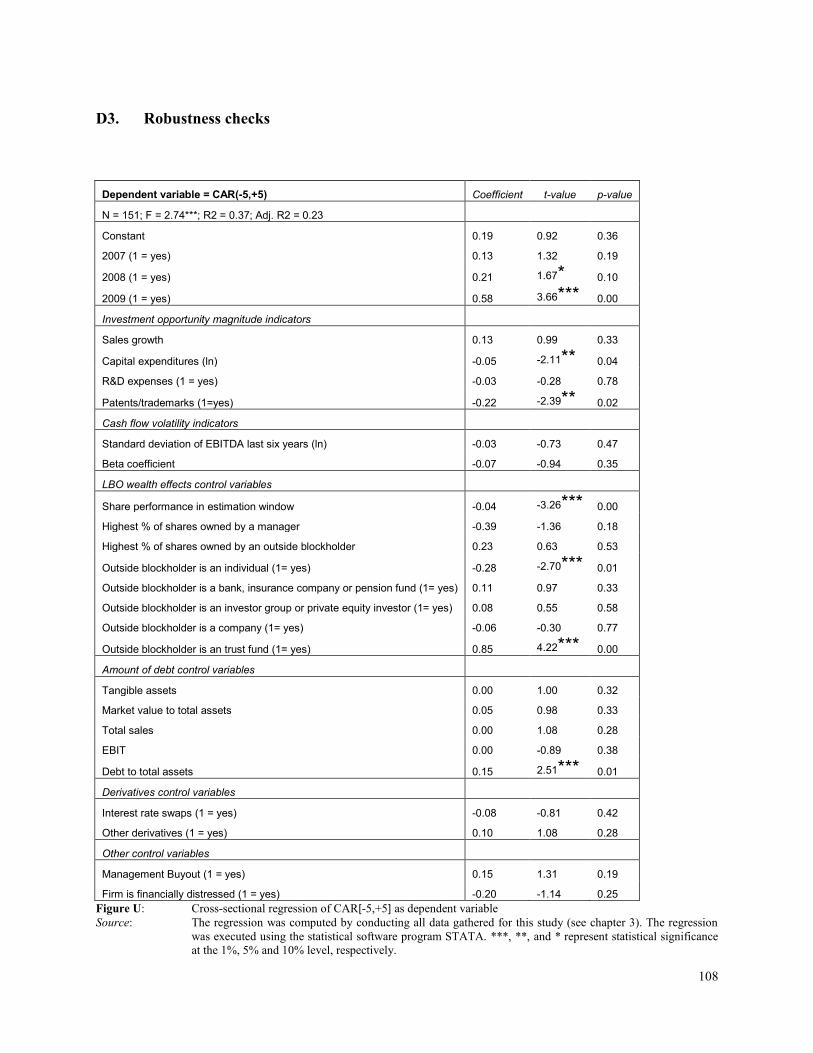
108

D3. Robustness checks

Dependent variable = CAR(-5,+5) Coefficient t-value p-value

N = 151; F = 2.74***; R2 = 0.37; Adj. R2 = 0.23

Constant 0.19 0.92 0.36

2007 (1 = yes) 0.13 1.32 0.19

2008 (1 = yes) 0.21 1.67* 0.10

2009 (1 = yes) 0.58 3.66*** 0.00

Investment opportunity magnitude indicators

Sales growth 0.13 0.99 0.33

Capital expenditures (ln) -0.05 -2.11** 0.04

R&D expenses (1 = yes) -0.03 -0.28 0.78

Patents/trademarks (1=yes) -0.22 -2.39** 0.02

Cash flow volatility indicators

Standard deviation of EBITDA last six years (ln) -0.03 -0.73 0.47

Beta coefficient -0.07 -0.94 0.35

LBO wealth effects control variables

Share performance in estimation window -0.04 -3.26*** 0.00

Highest % of shares owned by a manager -0.39 -1.36 0.18

Highest % of shares owned by an outside blockholder 0.23 0.63 0.53

Outside blockholder is an individual (1= yes) -0.28 -2.70*** 0.01

Outside blockholder is a bank, insurance company or pension fund (1= yes) 0.11 0.97 0.33

Outside blockholder is an investor group or private equity investor (1= yes) 0.08 0.55 0.58

Outside blockholder is a company (1= yes) -0.06 -0.30 0.77

Outside blockholder is an trust fund (1= yes) 0.85 4.22*** 0.00

Amount of debt control variables

Tangible assets 0.00 1.00 0.32

Market value to total assets 0.05 0.98 0.33

Total sales 0.00 1.08 0.28

EBIT 0.00 -0.89 0.38

Debt to total assets 0.15 2.51*** 0.01

Derivatives control variables

Interest rate swaps (1 = yes) -0.08 -0.81 0.42

Other derivatives (1 = yes) 0.10 1.08 0.28

Other control variables

Management Buyout (1 = yes) 0.15 1.31 0.19

Firm is financially distressed (1 = yes) -0.20 -1.14 0.25

Figure U: Cross-sectional regression of CAR[-5,+5] as dependent variable

Source: The regression was computed by conducting all data gathered for this study (see chapter 3). The regression

was executed using the statistical software program STATA. ***, **, and * represent statistical significance

at the 1%, 5% and 10% level, respectively.

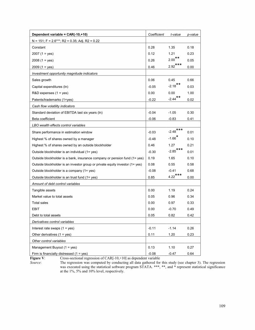
109

Dependent variable = CAR(-10,+10) Coefficient t-value p-value

N = 151; F = 2.6***; R2 = 0.35; Adj. R2 = 0.22

Constant 0.28 1.35 0.18

2007 (1 = yes) 0.12 1.21 0.23

2008 (1 = yes) 0.26 2.00** 0.05

2009 (1 = yes) 0.46 2.92*** 0.00

Investment opportunity magnitude indicators

Sales growth 0.06 0.45 0.66

Capital expenditures (ln) -0.05 -2.18** 0.03

R&D expenses (1 = yes) 0.00 0.00 1.00

Patents/trademarks (1=yes) -0.22 -2.44** 0.02

Cash flow volatility indicators

Standard deviation of EBITDA last six years (ln) -0.04 -1.05 0.30

Beta coefficient -0.06 -0.83 0.41

LBO wealth effects control variables

Share performance in estimation window -0.03 -2.48*** 0.01

Highest % of shares owned by a manager -0.48 -1.66* 0.10

Highest % of shares owned by an outside blockholder 0.46 1.27 0.21

Outside blockholder is an individual (1= yes) -0.30 -2.85*** 0.01

Outside blockholder is a bank, insurance company or pension fund (1= yes) 0.19 1.65 0.10

Outside blockholder is an investor group or private equity investor (1= yes) 0.08 0.55 0.58

Outside blockholder is a company (1= yes) -0.08 -0.41 0.68

Outside blockholder is an trust fund (1= yes) 0.85 4.22*** 0.00

Amount of debt control variables

Tangible assets 0.00 1.19 0.24

Market value to total assets 0.05 0.96 0.34

Total sales 0.00 0.97 0.33

EBIT 0.00 -0.70 0.49

Debt to total assets 0.05 0.82 0.42

Derivatives control variables

Interest rate swaps (1 = yes) -0.11 -1.14 0.26

Other derivatives (1 = yes) 0.11 1.20 0.23

Other control variables

Management Buyout (1 = yes) 0.13 1.10 0.27

Firm is financially distressed (1 = yes) -0.08 -0.47 0.64

Figure V: Cross-sectional regression of CAR[-10,+10] as dependent variable

Source: The regression was computed by conducting all data gathered for this study (see chapter 3). The regression

was executed using the statistical software program STATA. ***, **, and * represent statistical significance

at the 1%, 5% and 10% level, respectively.

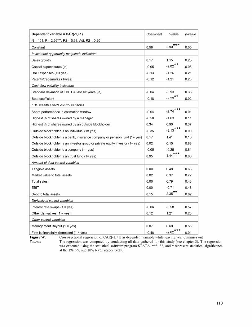
110

Dependent variable = CAR(-1,+1) Coefficient t-value p-value

N = 151; F = 2.66***; R2 = 0.33; Adj. R2 = 0.20

Constant 0.56 2.90*** 0.00

Investment opportunity magnitude indicators

Sales growth 0.17 1.15 0.25

Capital expenditures (ln) -0.05 -2.02** 0.05

R&D expenses (1 = yes) -0.13 -1.26 0.21

Patents/trademarks (1=yes) -0.12 -1.21 0.23

Cash flow volatility indicators

Standard deviation of EBITDA last six years (ln) -0.04 -0.93 0.36

Beta coefficient -0.18 -2.29** 0.02

LBO wealth effects control variables

Share performance in estimation window -0.04 -2.74*** 0.01

Highest % of shares owned by a manager -0.50 -1.63 0.11

Highest % of shares owned by an outside blockholder 0.34 0.90 0.37

Outside blockholder is an individual (1= yes) -0.35 -3.13*** 0.00

Outside blockholder is a bank, insurance company or pension fund (1= yes) 0.17 1.41 0.16

Outside blockholder is an investor group or private equity investor (1= yes) 0.02 0.15 0.88

Outside blockholder is a company (1= yes) -0.05 -0.25 0.81

Outside blockholder is an trust fund (1= yes) 0.95 4.44*** 0.00

Amount of debt control variables

Tangible assets 0.00 0.48 0.63

Market value to total assets 0.02 0.37 0.72

Total sales 0.00 0.79 0.43

EBIT 0.00 -0.71 0.48

Debt to total assets 0.15 2.35** 0.02

Derivatives control variables

Interest rate swaps (1 = yes) -0.06 -0.58 0.57

Other derivatives (1 = yes) 0.12 1.21 0.23

Other control variables

Management Buyout (1 = yes) 0.07 0.60 0.55

Firm is financially distressed (1 = yes) -0.48 -2.62*** 0.01

Figure W: Cross-sectional regression of CAR[-1,+1] as dependent variable while leaving year dummies out

Source: The regression was computed by conducting all data gathered for this study (see chapter 3). The regression

was executed using the statistical software program STATA. ***, **, and * represent statistical significance

at the 1%, 5% and 10% level, respectively.

111

D4. Description of independent variables

Abbreviation Short description Elaborate description

SGLYR Sales growth last year The sales growth is based on data from COMPUSTAT or the annual reports concerning net sales of the two years preceding the year of the first LBO announcement

LOGCAPEX Natural logarithm of capital expenditures

The capital expenditures are based on data from COMPUSTAT or the annual reports of the individual companies of the year preceding the year of the first LBO announcement.

RDEXP R&D expenses (1 = yes) R&D expenses are based on data from the annual reports of the individual companies of the year preceding the year of the first LBO announcement. Information on R&D expenses was available most often via the income statements of the individual companies.

PAT Patents or trademarks (1 = yes) Number of patents or trademarks are based on data from the annual reports of the individual companies of the year preceding the year of the first LBO announcement. Information on patents was available most often via the “Intellectual Property Rights” section of the annual reports of the companies (“Part 1 Item 1 Business” of the Annual Report).

LOGSTDE Natural logarithm of standard deviation of EBITDA last six years

The cash flow volatility is based on data from COMPUSTAT or the annual reports concerning EBITDA of the six years preceding the year of the first LBO announcement. The cash flow volatility represents the standard deviation of EBITDA over these six years.

BETA Beta coefficient The beta of the individual firms was calculated over the estimation period of our event study analysis

SPP Share performance in estimation window

The average yearly share performance of the individual firms was calculated over the estimation period of our event study analysis

112

HMO Highest % of shares owned by a manager

The information concerning is based on data from the proxy statements of the individual companies of the year preceding the year of the first LBO announcement.

HBHO Highest % of shares owned by an outside blockholder

The information concerning is based on data from the proxy statements of the individual companies of the year preceding the year of the first LBO announcement.

BHOI Outside blockholder is an individual (1= yes)

The information concerning is based on data from the proxy statements of the individual companies of the year preceding the year of the first LBO announcement.

BHOB Outside blockholder is a bank, insurance company or pension fund (1= yes)

The information concerning is based on data from the proxy statements of the individual companies of the year preceding the year of the first LBO announcement.

BHOPE Outside blockholder is an investor group or private equity investor (1= yes)

The information concerning is based on data from the proxy statements of the individual companies of the year preceding the year of the first LBO announcement.

BHOC Outside blockholder is a company (1= yes)

The information concerning is based on data from the proxy statements of the individual companies of the year preceding the year of the first LBO announcement.

BHOT Outside blockholder is an trust fund (1= yes)

The information concerning is based on data from the proxy statements of the individual companies of the year preceding the year of the first LBO announcement.

TANGA Tangible assets The tangible assets are based on data from COMPUSTAT or the annual reports of the individual companies of the year preceding the year of the first LBO announcement.

113

MVTA Market value to total assets The total market value of a firm was calculated by multiplying the number of common shares outstanding and the closing share price at the end of the year before the LBO announcement. Both the number of common shares outstanding and the closing share price are based on data from COMPUSTAT or the annual reports of the individual companies of the year preceding the year of the first LBO announcement.

TS Total sales The total sales are based on data from COMPUSTAT or the annual reports of the individual companies of the year preceding the year of the first LBO announcement.

EBIT EBIT The EBIT is based on data from COMPUSTAT or the annual reports of the individual companies of the year preceding the year of the first LBO announcement.

DTA Debt to total assets We calculated the total debt of a company by adding up its current liabilities and its long-term debt. Both the current liabilities and the long-term debt are based on data from COMPUSTAT or the annual reports of the individual companies of the year preceding the year of the first LBO announcement.

IRS Interest rate swaps (1 = yes) This dummy variable is based on data from the annual reports of the individual companies of the year preceding the year of the first LBO announcement. We obtained the data by exploring the entire digital annual reports of the companies on the keyword “Interest Rate Swap”. Information on interest rate swaps was available most often via Item 7 „Management‟s discussion and analysis of financial condition and results of operation‟ of the annual reports of the individual companies (Section “Debt and Liquidity”).

OD Other derivatives (1 = yes) This dummy variable is based on data from the annual reports of the individual companies of the year preceding the year of the first LBO announcement. We obtained the data by exploring the entire digital annual reports of the companies on the keyword “Derivative”. Information on derivatives was available most often via Item 7 „Management‟s discussion and analysis of financial condition and results of operation‟ of the annual reports of the individual companies (Section “Debt and Liquidity”).

2007 2007 (1 = yes) Information on announcement dates was collected via the SDC database

2008 2008 (1 = yes) Information on announcement dates was collected via the SDC database

114

2009 2009 (1 = yes) Information on announcement dates was collected via the SDC database

MBO Management Buyout (1 = yes) Information on deal type was collected via the SDC database (deal synopsis)

FD Firm is financially distressed (1 = yes)

Information on whether a firm was financially distressed was collected via the SDC database (target bankrupt)

Figure X: Description of independent variables

115

Appendix E Non-completed deals

E1. Comparison of CAARS of completed and non-completed deals

CAAR(-1,+1) CAAR (-5,+5)

Completed deals 23.49% 23.40%

Non-completed deals 21.74% 24.70%

Figure Y: Comparison of CAARS of completed and non-completed deals in event windows [-1,+1] and [-5,+5] Source: Share price information from Datastream, information on the market index proxy (CRSP equally-weighted

daily returns on the S&P 500 index excluding dividends) and the three-month Treasury Bill rate from the

CRSP database, announcement dates from the SDC database and own calculations.

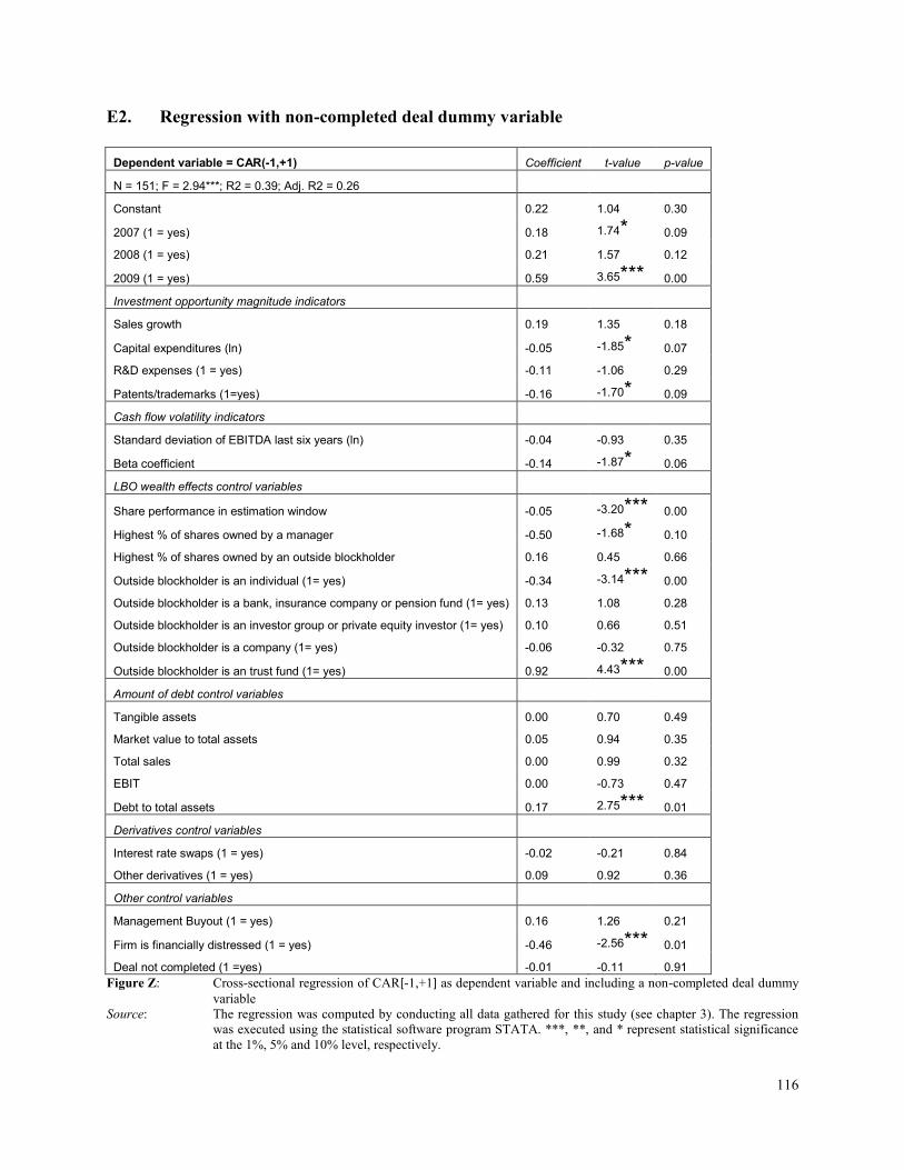
116

E2. Regression with non-completed deal dummy variable

Dependent variable = CAR(-1,+1) Coefficient t-value p-value

N = 151; F = 2.94***; R2 = 0.39; Adj. R2 = 0.26

Constant 0.22 1.04 0.30

2007 (1 = yes) 0.18 1.74* 0.09

2008 (1 = yes) 0.21 1.57 0.12

2009 (1 = yes) 0.59 3.65*** 0.00

Investment opportunity magnitude indicators

Sales growth 0.19 1.35 0.18

Capital expenditures (ln) -0.05 -1.85* 0.07

R&D expenses (1 = yes) -0.11 -1.06 0.29

Patents/trademarks (1=yes) -0.16 -1.70* 0.09

Cash flow volatility indicators

Standard deviation of EBITDA last six years (ln) -0.04 -0.93 0.35

Beta coefficient -0.14 -1.87* 0.06

LBO wealth effects control variables

Share performance in estimation window -0.05 -3.20*** 0.00

Highest % of shares owned by a manager -0.50 -1.68* 0.10

Highest % of shares owned by an outside blockholder 0.16 0.45 0.66

Outside blockholder is an individual (1= yes) -0.34 -3.14*** 0.00

Outside blockholder is a bank, insurance company or pension fund (1= yes) 0.13 1.08 0.28

Outside blockholder is an investor group or private equity investor (1= yes) 0.10 0.66 0.51

Outside blockholder is a company (1= yes) -0.06 -0.32 0.75

Outside blockholder is an trust fund (1= yes) 0.92 4.43*** 0.00

Amount of debt control variables

Tangible assets 0.00 0.70 0.49

Market value to total assets 0.05 0.94 0.35

Total sales 0.00 0.99 0.32

EBIT 0.00 -0.73 0.47

Debt to total assets 0.17 2.75*** 0.01

Derivatives control variables

Interest rate swaps (1 = yes) -0.02 -0.21 0.84

Other derivatives (1 = yes) 0.09 0.92 0.36

Other control variables

Management Buyout (1 = yes) 0.16 1.26 0.21

Firm is financially distressed (1 = yes) -0.46 -2.56*** 0.01

Deal not completed (1 =yes) -0.01 -0.11 0.91

Figure Z: Cross-sectional regression of CAR[-1,+1] as dependent variable and including a non-completed deal dummy

variable

Source: The regression was computed by conducting all data gathered for this study (see chapter 3). The regression

was executed using the statistical software program STATA. ***, **, and * represent statistical significance

at the 1%, 5% and 10% level, respectively.