The relationship between crude oil prices and stock markets in ...

The relationship between

crude oil prices and stock

markets in Sweden and Norway

Petter Hälldahl, Mohammad Refaet Rahman

Department of Business Administration

Master's Program in Finance

Master's Thesis in Business Administration I, 15 Credits, Spring 2020

Supervisor: Dennis Sundvik

ii

[THIS PAGE WAS INTENTIONALLY LEFT BLANK]

iii

Preface This 1st year's master’s Thesis 15 ECTS has been made at Umeå University during the latter

part of the spring term year 2020. Most of the work on the thesis has been made from

distance since the current Covid-19 has its effects.

First of all, the authors, Petter Hälldahl and Mohammad Refaet Rahman, would like to

greatly thank our supervisor Dennis Sundvik for his time and support. During the progress

concrete and creative suggestions have been given for which we are very thankful.

Thanks a lot!

iv

Abstract In this study, the authors examined the relationship between crude oil price and the Swedish

and Norwegian stock markets. Using linear regression models the authors found that the

Swedish stock market and Norwegian stock market both have a positive relation with crude

oil price. This supports the hypothesis that crude oil price has a positive impact on

Norwegian stock market, since Norway is an oil exporting country. However, this result

contradicts a hypothesis of a negative relationship for an oil importing country like Sweden.

The authors also looked into the relationship between exchange rates (Swedish krona and

Norwegian krone) and oil price, which reveals that oil price is significantly negatively

correlated with Swedish krona and Norwegian Krone. The study contributes with evidence

from underexplored regions of the world.

Keywords: oil price, stock market, exchange rate, financial markets

Abbreviation and explanation list

Diff Difference measured in significance and coefficients between two variables

OMXSPI All listed stocks on the OMX Nordic Exchange Stockholm

OSEBX All listed stocks on the Oslo stock exchange

USD American Dollar

USD/SEK 1 US dollar in Swedish kronor

USD/NOK 1 US dollar in Norwegian crowns

SWE Sweden

SEK Swedish krona

NOK Norwegian krone

NOR Norway

v

Table of contents 1. Introduction 1

1.1 Problem background 1

1.2 Problem and research questions 2

1.3 Purpose 2

1.4 Delimitations 2

2. Theoretical framework 3

2.1 Oil price 3

2.2 Stock market 5

3. Prior studies 6

3.1 Empirical literature review 6

3.2 Formulation of hypothesis 9

3.2.1 Oil price relationship to Swedish stock market 9

3.2.2 Oil price relationship to Norwegian stock market 9

3.3 Analysis model 10

4. Method 11

4.1 Literature gathering and source criticism 11

4.2 Method and research design 11

4.3 Sampling 12

4.4 Collection of data 12

4.5 Definitions of the variables 12

4.5.1 Oil price 13

4.5.2 Swedish stock market 13

4.5.3 Norwegian stock market 13

4.5.4 Swedish exchange rate 13

4.5.5 Norwegian exchange rate 13

4.6 Model specification 13

4.7 Statistical processing 14

4.8 Validity and reliability 15

4.9 Ethical approach 16

5. Results and analysis 17

5.1 Graphs and descriptive statistics 17

5.1.1 Graphs 17

5.1.2 Descriptive statistics 18

5.2 Correlation matrix 19

5.2.1 Correlation matrix for monthly observations 20

vi

5.2.2 Correlation matrix for daily observations 21

5.3 Multiple linear regression 22

5.3.1 Multiple linear regression for monthly observations 23

5.3.2 Multiple linear regression for daily observations 25

5.3.3 Significance of difference in coefficients 28

5.3.4 Robustness test 29

5.4 Multicollinearity 30

5.5 Analysis 31

5.6 Results of hypothesis 32

6. Conclusion and proposal for future studies 33

6.1 Conclusion 33

6.2 Limitations and proposal for future studies 33

6.3 Generalizability 34

Table list

Table 1. Compilation of hypotheses 10

Table 2. Descriptive statistics of monthly data 18

Table 3. Descriptive statistics of daily data 19

Table 4. Monthly correlation matrix for data measured by level of the variables 20

Table 5. Monthly correlation matrix for data measured by changes of the variables 20

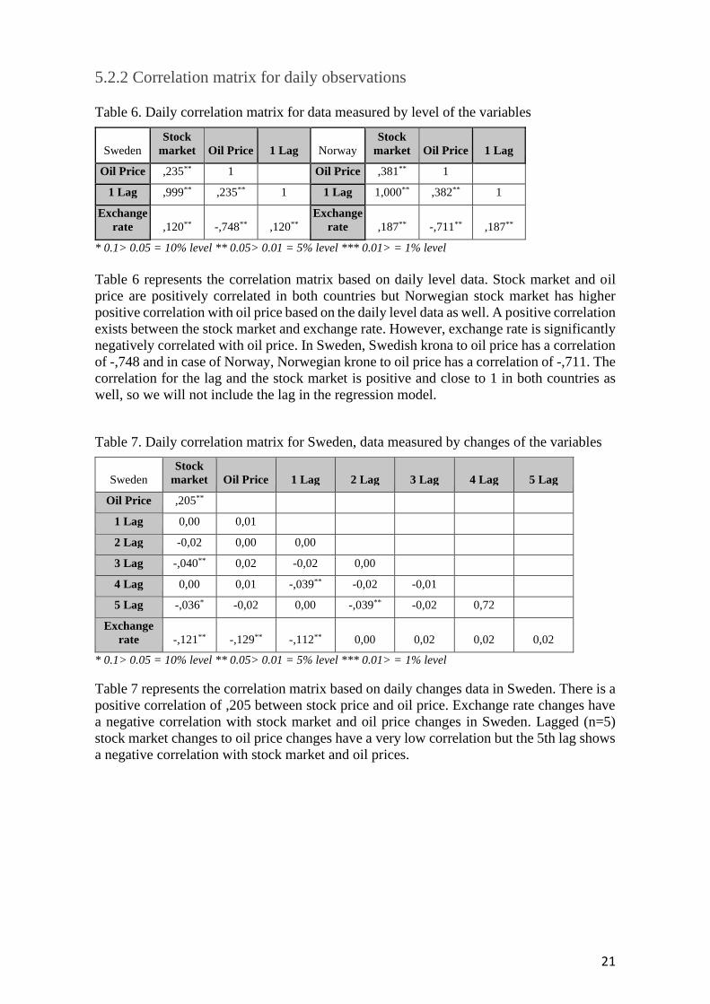
Table 6. Daily correlation matrix for data measured by level of the variables 21

Table 7. Daily correlation matrix for Sweden, data measured by changes of the variables

21

Table 8. Daily correlation matrix for Norway, data measured by changes of the variables

22

Table 9. Monthly regression for data measured by level of the variables 23

Table 10. Monthly regression for data measured by changes of the variables 24

Table 11. Daily regression for data measured by level of the variables 25

Table 12. Daily regression for data measured by changes of the variables 26

Table 13. Test of difference in coefficients on daily observations 28

Table 14. Test of difference in coefficients on monthly observations 29

Table 15. Summary of hypothesis testing 32

Figure List: Figure 1. Analysis model 10

Figure 2. Historical price movement of oil price, stock market in Sweden (OMXSPI) and

stock market in Norway (OSEBX). 17

1

1. Introduction

In the introductory chapter the focus is on presenting the problem background and previous

research concerning the relationship between oil price changes and stock markets. The

introduction also focuses on previous research on the oil price relationship with exchange

rates. The problem focuses on the lack of research in Sweden dealing with the oil price

relationship with the stock market. Then this is formulated into a problem and a purpose of

the study. Lastly, the limitations of the research are presented.

1.1 Problem background

Crude oil price plays a key role in the world economy and the impact of crude oil price

fluctuation has always been a matter of concern to the economists (Barsky and Kilian, 2004;

Hamilton, 1996, 2003; Hooker, 1996; Kilian, 2008, 2009; Kilian and Park, 2009; Wang et

al. 2013). Since World War II, crude oil price hikes were responsible for all the recessions

except one in the United States (Bjørnland, 2009). The authors of this study believe that

crude oil price plays a vital role in the Swedish and Norwegian economy as well.

Researchers have considered oil price as an underlying factor for stock market volatility

(Sadorsky, 1999; Cuñado and Perez de Gracia, 2003; Park and Ratti, 2008; Apergis and

Miller, 2009; Kilian and Park, 2009; Zhang and Asche, 2014). Some researchers concluded

that there is a positive relationship between crude oil price and stock markets whereas some

found that there is a negative correlation between crude oil price and stock markets (Badeeb

and Lean, 2018; Fang and Egan, 2018; Filis et al. 2011; Nath Sahu et al., 2014; Wang et al.,

2013). Although many researchers examined the relationship between oil price and

Norwegian stock market, there are only a few researches that examined the impact of oil

price change on the Swedish stock market. The correlation between stock price and oil price

is ambiguous and the reason behind this can be the underlying reason behind oil price

change (Bjørnland, 2009). Hence, the authors would like to examine the association

between crude oil price and the Swedish stock exchange and Norwegian stock exchange in

this research.

The Stockholm stock exchange, which is formally known as Nasdaq Stockholm, is

Sweden’s main stock exchange. It was established back in 1863. Currently there are 368

companies that are listed in the stock exchange (Nasdaq, 2020a). Oslo stock exchange is the

main stock exchange of Norway which is also known as Oslo Børs. It was founded in 1819.

In Oslo Børs, 198 companies are currently listed (Oslo Børs, 2020a).

Exchange rate is one of the most important macroeconomic factors. It has always been an

influential macroeconomic factor which has a huge impact on every economy (Alley, 2018).

After the first oil price shock back in 1973, Hamilton’s (1983) influential seminal paper first

revealed that crude oil price and other macro economic factors are largely connected. Since

crude oil is related to export and import activities, the authors of this thesis will include

controls for the exchange rate of Norway and Sweden in this research paper.

2

1.2 Problem and research questions

Due to Covid-19, crude oil prices went down drastically and this may change the world’s

economic order (David, 2020). A price war and a ploughing demand for crude oil brought

down oil price from 70$ per barrel in December, 2019 to around 20$ per barrel in April,

2020 which put the industry in survival mode (Carrington et al., 2020). As oil price hit 20

years low, two third of the annual investment amounting 130 billion US dollar in the oil

industry was halted and major stock market valuations came down heavily since January,

2020 (Carrington et al., 2020). Many research works can be found which try to find the

impact of the crude oil in the large economies like the United States, China etc. and its

impact on the stock exchanges. But there are only a few research works which show the

impact of crude oil price fluctuations in Swedish stock exchange and Norwegian stock

exchange. Therefore, the authors of this study would like to explore this area and try to

answer following research questions:

- What is the relationship between oil price and the Swedish stock market?

- What is the relationship between oil price and the Norwegian stock market?

An additional research question that will be examined is whether the relationship between

the oil price and the stock market is different in Norway from Sweden. This questions is

grounded in the fact that Norway is an oil exporting country whereas Sweden is an oil

importing country.

1.3 Purpose

The main purpose of this study is to examine the relationship of crude oil price with Swedish

stock market and Norwegian stock market. A sub-purpose is to examine whether the

relationship is different for oil importing and oil exporting economies.

1.4 Delimitations

First delimitation of this study is that authors took sample data from 2000 to 2019. The

authors used the stock market index and oil price of the last 20 years for data analysis and

research. This makes the study more focused on the 21st century which leaves out

information before that. So, there will be a bit of sampling bias in this case.

Second delimitation of this study is the lack of prior studies on the impact of oil price on

Swedish stock market. Only a few researchers worked on this topic. The authors needed to

find research papers which contained research on this topic on some other comparable

countries and used those in the prior studies to formulate the hypothesis.

Last but not the least delimitation of the study is that the research is limited to the

Scandinavian region, to be more precise within Sweden and Norway. The authors wanted

to work with all the four Scandinavian countries. However, time is a major constraint for

the authors. Due to time shortage, the study only covers two countries.

3

2. Theoretical framework

In this chapter the underlying theories of the variables included in the study are described.

It begins by describing the independent variable oil price. After that the dependent variable

stock market is described. Finally, the control variable exchange rate is described which is

also an independent variable.

2.1 Oil price

Crude oil, one kind of fossil fuel, is an unrefined petroleum product which is comprised of

hydrocarbons and other organic materials (Chen, 2020). Refining the crude oil, it can be

converted into different kinds of usable products such as diesel, petrol, gasoline etc. (Chen,

2020). Amaded (2019) concluded that roughly 1.73 trillion barrels were the worlds’ proven

oil reserves in 2018 which can meet the oil demand for the next 50 years. Venezuela, Saudi

Arabia and Canada tops in the worlds’ oil reserves and these three countries have a 17.5%,

17,2% and 9.7% of total oil reserves in the world respectively. In 2019, China, USA and

India were the top oil importing countries in the world whereas Saudi Arabia, Russia and

Iraq were top oil exporting countries during this period (Workman, 2020).

Oil price has always been a matter of concern for the world economy. Predicting the oil

price is one of the hardest tasks for the analysts. Western countries believe that oil price is

still linked to the development that took place back in 1970 and 1980 with the emergence

of persian gulf countries and OPEC nations (Carollo, 2012). So, the base of the oil price

index was laid in the 1970s. Main factors that affect the oil price are oil supply and demand,

oil production cost, oil inventory levels and US dollar exchange rate (Li and Liu, 2011).

During 1973-1974, oil price fluctuation was caused by Arab-Israel war. Iranian revolution

in 1978 and global financial crisis in 2008 also caused oil price hikes (Radetzki, 2012). If

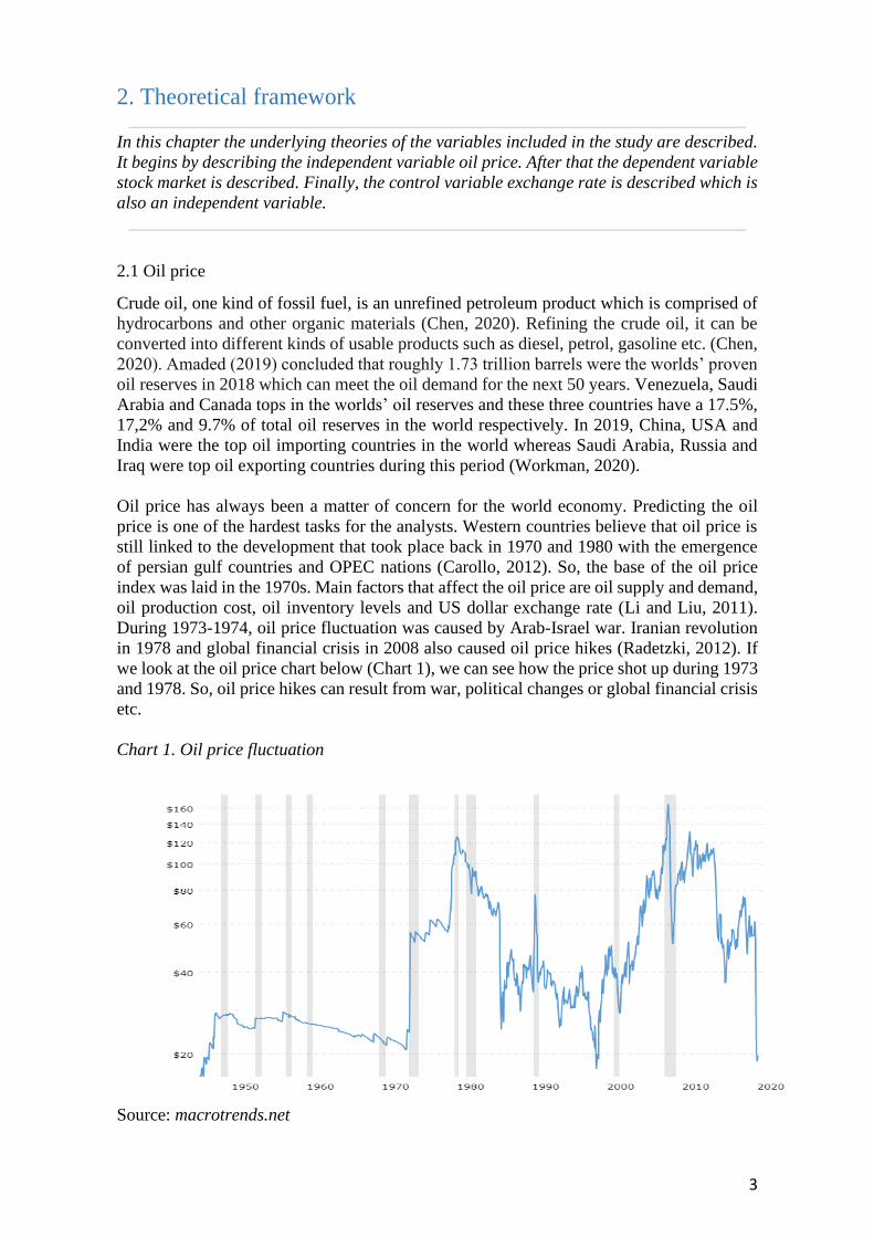
we look at the oil price chart below (Chart 1), we can see how the price shot up during 1973

and 1978. So, oil price hikes can result from war, political changes or global financial crisis

etc.

Chart 1. Oil price fluctuation

Source: macrotrends.net

4

Islamic Republic of Iran, Venezuela, Kuwait, Saudi Arabia and Iraq founded the

Organization of the Petroleum Exporting Countries (OPEC) in 1960 (OPEC, 2020). Later

Qatar, Indonesia, Libya, the United Arab Emirates, Algeria, Nigeria, Gabon, Angola,

Equatorial Guinea and Congo joined the cartel (OPEC, 2020). OPEC produces

approximately 44% of the total crude oil production (Garside, 2019). OPEC tries to control

the oil price by manipulating the supply and demand of the oil (Radetzki, 2012). Marginal

revenue for OPEC is calculated subtracting the marginal revenue which the group would

lose if it had to lower the price to all its prior clients from that marginal barrel (Hamilton,

2009). On the other hand, deducting the lost revenue to the member from the price would

give the marginal revenue for the OPEC members (Hamilton, 2009). As a result, there is an

arbitrary profit for the member countries if they produce a little more than the group agreed

(Hamilton, 2009).

Unexpected fluctuations in the supply of the crude oil negatively affect the prices (Fawley

et al., 2012). For example, oil prices will go up if OPEC decides to cut the production

unexpectedly. Higher demand for oil can also put pressure on the oil price. A growing world

economy leads to higher demand for industrial commodities such as crude oil (Fawley et

al., 2012). Higher demand for crude oil in emerging markets like China and India pushes

the global oil demand and its price (Fawley et al., 2012). A rise in oil production increases

the supply of oil in the market which sometimes causes oil price to drop. Growing foreign

exchange value of the US dollar can affect the oil price as well (Demirbas et al., 2017).

Historically it has been seen that a stronger US dollar value negatively affects the oil price

(Demirbas et al., 2017). Kilian (2009) concluded that China and India have more influence

on the oil price hike in recent years.

It is statistically proved that oil prices follow a random walk without drift (Hamilton, 2009).

But analysts might have more success on shorter samples and doing more detailed analysis,

but predicting the long term oil price is not that easy (Hamilton, 2009).

Speculation on crude oil price is possible in the financial market (Hamilton, 2009).

According to Fawley et al. (2012), speculation is buying something today with a hope to

sell it at a higher price in the future. Speculation on oil prices in the financial market can be

done in the following way: Investors purchase a future contract on oil to be exercised at a

future date and sell the future contract before maturity or expiration and then buys another

futures contract with a more distant maturity date expecting that the price of the crude oil

will go up in the future (Fawley et al., 2012). Thus, the demand for the crude oil futures

contracts rises which eventually pushes up the futures price and this moves the spot crude

oil price (Fawley et al., 2012).

From the above discussion, we can summarize that the supply and demand of crude oil can

be disrupted automatically due to political policy changes, war, interference of OPEC,

speculation or financial crisis. Different macroeconomic factors are affected by this reason

and oil prices spike up or go down. Global macroeconomic factors influence the oil supply

and demand.

5

2.2 Stock market

The stock market is a place where companies issue shares to the investors through initial

public offering to raise share capital and stocks of these publicly listed firms are traded

(Economic Times, 2020). Stock markets give opportunities to the investors to increase their

assets (Zhang et al., 2014). Every stock market has its own index. A market index is

basically a smaller subset of the stock market which helps the stakeholders compare the

current performance with past performance (Caplinger, 2020). The index can be of different

types such as price weighted index, market-capitalization-weighted index, equal-weight

index. When indexes give more weight to higher stock prices firms, it is called price

weighted index (Caplinger, 2020). Indexes which give more weight to larger capitalized

companies are called market-capitalization-weighted indexes. Nasdaq Composite and S and

P 500, both are market capitalization based indexes where big companies like Apple and

Microsoft get more weight compared to small companies (Caplinger, 2020). Another type

of index is equity weighted index. In this index, weight is equally assigned to all the stocks

of the market (Caplinger, 2020).

Information about future prospects and current economic conditions of the firms determine

the asset prices on the stock market (Bjørnland, 2009). Many researchers examined the

relationship between the stock market and macroeconomic factors (Bastianin et al.., 2016).

In the seminal work of Campbell (1991), shows that stock market fluctuation depends on

both financial variables like crude oil price and macroeconomic factors such as interest rate,

inflation rate, exchange rate etc. which laid the theoretical foundation of the relationship

(Bastianin et al., 2016). Geske and Roll (1983) argued that stock returns tend to reflect real

economic activities, where unexpected negative stock returns could signal an increase in

expected inflation. According to Basher et al. (2018), “The price of a share in a company is

equal to the expected present value of discounted future cash flows.” Current and future

cash flow of a company can be affected by crude oil price fluctuations as price volatility in

the crude oil market affects the interest rate (Basher et al. 2018). So, different

macroeconomic factors and oil price fluctuations play key roles in stock market volatility.

From an investor's point of view, assets that are positively correlated but not perfectly

correlated is seen as diversification. The opposite correlation (negative) or a non-correlated

asset creates a hedge (Baur and Lucey, 2010).

6

3. Prior studies

This chapter describes the empirical literature review where research is shown concerning

the relationship of oil price and stock market. After that formulations of hypotheses are

shown for the relationship between oil price and stock market. Finally, this chapter ends up

with showing an analysis model that has been developed.

3.1 Empirical literature review

In this part the previous research on the connection between oil price and stock prices is

presented. The main focus is on describing earlier studies of oil price relationship to stock

markets in importing and exporting countries. There is a lot of research regarding the

relationship between oil price and stock markets. There exist ambiguous results regarding

the relationship and correlation between the variables and what causes the variables to

change their value. The reason for this could be due to what Bjørnland (2009) mentions

where the effect could come from an underlying change in oil price and not from the stock

market. Killin (2009) also concluded that the impact of crude oil fluctuation depends on the

underlying reasons behind the crude oil price fluctuation.

Although, some of the previous research found a positive relationship between oil price and

stock market (Badeeb and Lean, 2018; Fang and Egan, 2018; Oskooe, 2012; Filis et al.,

2011; Nath Sahu, et al. 2014). The relationship is positive according to Badeeb and Lean

(2018) in the short run, and stock market indices react in a linear manner with oil price

changes. Another aspect that may be of importance when research has been done is what

kind of industries the stocks included are based on. For instance, Fang and Egan (2018)

finds that stock market returns of the coal, chemical, mining and oil industries are positively

affected by crude oil price movements. So, the relationship depends a lot of what the stocks

in the market indices are built by, therefore the correlation and relationship differ in prior

research. When looking into the method of using percentage changes in oil price and stock

markets Oskooe, (2012) finds a positive weak relationship. An interesting point that the

article also finds is that variance of oil price fluctuations does not cause the variance in stock

returns. This was found when the research was done in Iran 1999 to 2010 using weekly data

(Oskooe, 2012). Another article that finds that the relationship can be both negative and

positive due to different factors is one by Filis et al. (2011). The positive relationship was

mainly found when the oil price shocks were in demand for oil, and then had a positive

effect on the stock market. This in comparison to the negative relationship that exists when

there is a shock in supply of oil, which led to a negative effect on the stock market. Their

study results are based on exporting countries such as Canada, Mexico and Brazil. And

importing countries such as USA, Germany and Netherlands over the period 1987 to 2009

using monthly data (Filis et al., 2011). Lastly there is a research by Nath Sahu et al. (2014)

that finds a positive long run relationship between oil prices and the movement of stock

market indices. This was found when they examined the relationship during 2001 to 2013

using daily data in India. (Nath Sahu et al, 2014) Another research by Nwosa (2014) have

found that oil prices have a significant relationship with the stock market in the long run

and that the stock market and oil price are cointegrated.

Even though there is research showing that the relationship between oil price and stock

market is positive due to different reasons, there is also research showing that a negative

relationship exists (Badeeb and Lean, 2018; Fang and Egan, 2018; Filis et al. 2011; Nath

Sahu et al., 2014; Wang et al., 2013). To be more specific, Badeeb and Lean, 2018 found a

negative relationship in the long run. This research was based in the Middle East from 1996

7

to 2016 using monthly data. The research shows that stocks gain from a decline in oil price

(Badeeb and Lean, 2018). A similar result was found by Nath Sahu et al., (2014) where the

result showed that an increase in the oil price led to negative effects on the stock market.

One aspect in that research is that oil-exporting economies have the opposite whereas an

increase in oil price leads to a positive effect on the stock market (Nath Sag hu et al., 2014).

This research has some similarities with the research by Wang et al., (2013) where

uncertainties in oil supply leads to negative effects on oil-importing economies and their

stock markets. There is also another aspect to see if a stock market has a positive or negative

relationship to oil price changes. A research by Fang et al. (2018) which was mentioned in

the paragraph above regarding what kind of industries that achieved a positive relationship.

Their research has also stated that there exist negative relationships to some industries such

as electronics, food manufacturing, general equipment, pharmaceuticals, retail, rubber and

vehicle industries. So, these industries have negative effects when the price of crude oil

changes. What Fang et al. (2018) research then shows that depending on what a stock market

index contains, it will have different effects when oil price changes due to if the industry is

positively or negatively related. Finally, there is a research of Filis et al., (2011) that found

a negative relationship between oil price and stock market when using the variables as

lagged. These negative relationship results were both found in importing countries and

exporting countries of oil (Filis et al., (2011).

So, there are both positive and negative relationships that have been found in previous

research regarding the relationship between oil price and stock market. But there is also

some prior research that has found a non-existing relationship between the variables. For

example, a research of Louis and Balli (2014) finds a low degree of relationship between

oil price and stock market. There is also another earlier research of Nath Sahu et al., (2014)

that mentions a non-existing relationship at all. What that research found was that prices of

crude oil have no significant causal effect on Indian stock market. That research was based

on daily observations from 2001 to 2013 using daily data and methods as Johansen’s

cointegration test, VECM, IRFs and VDCs (Nath Sahu et al., 2014).

From the above discussion it is evident that many researchers studied the relationship

between oil price and stock markets. Some researchers argued there is a positive relationship

between the stock market and crude oil price and some researchers also argued there is a

negative relationship between the stock market and crude oil price. Amid this ambiguity,

Wang et al. (2013) found that stock market return of a country in response to crude oil price

fluctuation depends on the countries’ position in the crude oil market and also on the factors

that drive the crude oil price. Marashdeh and Afandi (2017) also found the same result in

their research and concluded that the relationship between stock market and oil prices is

likely to depend on whether the countries are net importers of oil or net exporters of oil.

China, India, Italy, France, Germany and Korea are oil importing countries and Canada,

Mexico, Saudi Arabia, Norway, Venezuela, Russia and Kuwait are oil export oriented

countries (Wang et al., 2013).

According to Li et al. (2012), China is one of the major oil importing countries. The Chinese

stock market and oil prices have a negative correlation in the long run. Zhu et al. (2015)

argued that crude oil price sensitivity to Chinese stock market changes over time and it

changes by industry. Cong et al. (2008) studied the sensitivity of oil price fluctuation to

Chinese stock market for the time period of 1986 to 2005 and they concluded that there is

no significant relationship between Chinese stock market and crude oil price. According to

these researches Chinese stock market is less sensitive to crude oil price fluctuation.

8

Zhang and Asche (2014) studied the Nordic market and concluded that a positive

relationship exists between crude oil price and each Nordic stock market. Despite being oil

importing countries, three Nordic countries (Sweden, Finland and Denmark) move in the

same direction in the long run. Norway, a net oil exporter, has benefited from the oil price

hike which helped the country’s economic growth in the short run (Bjørnland, 2009). Basher

et al. (2018) concluded that a sudden rise in the idiosyncratic oil-market shocks on the stock

market is statistically significant for Norway. Zhang and Asche (2014) also expected that

an oil price hike has a positive effect on the oil-exporting country like Norway. Hammoudeh

and Li (2005) studied two oil-exporting countries (Mexico and Norway) to determine the

oil sensitivity and they found that an increase in oil prices has a positive impact on the stock

market in oil-exporting countries.

Bildirici and Badur (2018) found that India, an oil importing country, has a bidirectional

causality from crude oil price to stock market. Higher oil prices may increase the production

cost in the oil importing countries and stock market return can decline due to lower

profitability and dividend which means higher oil price has a negative impact on the Indian

capital market (Fang and You, 2014).

Canada, also a net-oil exporter, acts more in line with the oil importing countries as its

economy shows declining growth with a hike in the crude oil price (Basher et al., 2018).

Sadorsky (2001) indicated that there is a positive relationship between the price of crude oil

and oil and gas equity index in Canada. A probable reason behind this can be what Wang et

al. (2013) explained as, a rise in the oil price can also increase the production cost in Canada

as it is one of the top oil consuming countries. However, Basher et al. (2018) concluded

that oil inventory shock which is a “speculative component” of the real price of oil can have

a statistically significant impact on stock market return in Canada.

A rise in the oil price leads to higher production costs in oil importing countries resulting in

less disposable income for those countries and oil exporting countries will have a positive

economic effect as their income will rise from the high oil price (Bjørnland, 2009). In the

oil importing countries, oil price hike affects the production output and reduces usage of

energy in production. Because a rise in oil price leads to an increase in cost of production

which forces the firms to produce less. This reduction in production of goods and lower

income in oil importing countries leads to less consumption and investment spending which

reduces aggregate demand and supply (Bohi, 1989). Huge amount of empirical research

shows that oil price hikes have significantly adverse consequences for the world economy

(Hamilton, 1983); (Burbidge and Harrison, 1984); (Bjørnland, 2000); and (Hamilton, 2003).

However, this theory was challenged for the first time in 1986 following an oil price collapse

in the international market. Some researchers re-examined the previous results and and

found a negative relation between oil price and oil importing economies (Mork, 1989);

(Mork et al., 1994); (Lee et al., 1995); Hamilton (1996, 2003).

In case of oil exporting countries, an increase in oil price can affect the economy in two

ways. First, with positive wealth and income effects and second, with negative trade effects

(Bjørnland, 2009). An increase in oil price tunnels wealth from oil importers to oil exporters

which increases the money circulation in the domestic economy. However, inflation and

domestic currency value may go up due to this high level of monetary activities which is

good for the oil exporting countries (Haldane, 1997). Due to the rise in the oil price hike,

oil importing shall face economic pressure and they shall reduce their import due to

economic downturn (Bjørnland, 2009). But the net effect of both positive wealth effect and

negative trade effect remains unequivocal (Bjørnland, 1998, 2000).

9

The Appendix provides a summary of the prior studies, where in the result column the

relationship is bolded.

3.2 Formulation of hypothesis

In this chapter hypotheses are formulated based on previous research of the relationship

between oil price and stock market. The hypotheses are based on that oil price is an

independent variable and the stock markets in Sweden and Norway are dependent variables.

3.2.1 Oil price relationship to Swedish stock market

In this study the authors recognize Sweden as an importer of oil. It has very little oil

production in their own country which forces the country to import oil from other countries.

Data from JodiOil (2019) shows that Sweden's net-result for 2019 was negative (-4 065)

measured by thousand barrels per day. This was done by netting the difference between

export and import oil. As rise in the oil price leads to higher production costs in oil importing

countries resulting in less disposable income for those countries which shall have adverse

effect on share price and profitability of the firms (Bjørnland, 2009). India, an oil importing

country, has a negative relation between oil price and stock market (Fang and You, 2014).

Therefore, the conclusions from previous research lead to the following hypothesis:

H1: There is a negative relationship between oil price and the stock market in Sweden

Thus, the null hypothesis is that there is no relationship between oil price and the stock

market in Sweden.

3.2.2 Oil price relationship to Norwegian stock market

In this study the authors recognize Norway as an exporter of oil. Data from JodiOil, (2019)

shows that Norway in 2019 net-result was positive (14 059) measured by thousand barrels

per day. Since Norway is a net-exporter the economy as a whole and also the stock market

depends a lot on the oil price and its fluctuations. Hammoudeh and Li (2005) did a research

on the Mexican and the Norwegian stock market where they found that oil price increase

led to a positive effect on the stock markets in oil-exporting countries. That research is also

in line with prior studies where Bjørnland (2009), Basher et al. (2018) and Zhang and Asche

(2014) all found positive relationships between oil price and stock markets in oil-exporting

countries. Therefore, the conclusions from previous research lead to the following

hypothesis:

H2: There is a positive relationship between oil price and the stock market in Norway

Thus, the null hypothesis is that there is no relationship between oil price and the stock

market in Norway.

10

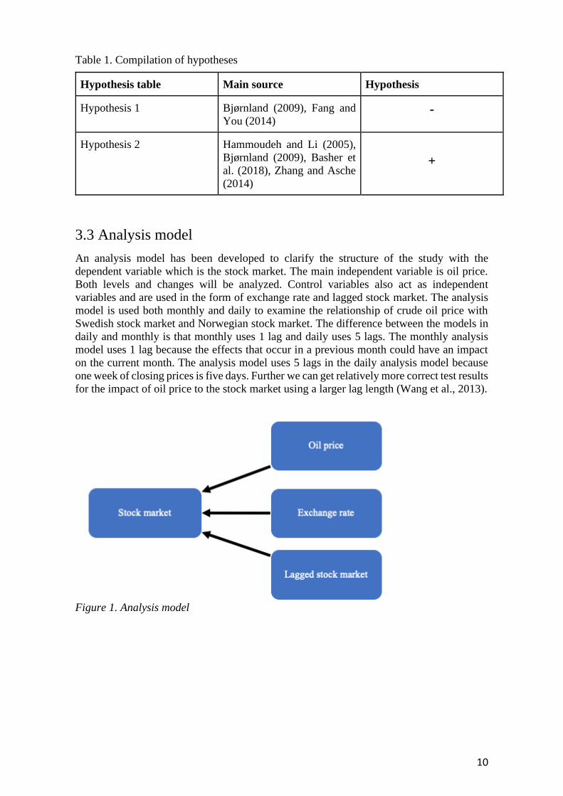
Table 1. Compilation of hypotheses

Hypothesis table Main source Hypothesis

Hypothesis 1 Bjørnland (2009), Fang and

You (2014) -

Hypothesis 2 Hammoudeh and Li (2005),

Bjørnland (2009), Basher et

al. (2018), Zhang and Asche

(2014)

+

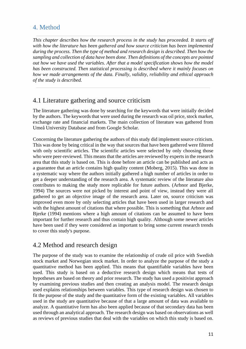
3.3 Analysis model

An analysis model has been developed to clarify the structure of the study with the

dependent variable which is the stock market. The main independent variable is oil price.

Both levels and changes will be analyzed. Control variables also act as independent

variables and are used in the form of exchange rate and lagged stock market. The analysis

model is used both monthly and daily to examine the relationship of crude oil price with

Swedish stock market and Norwegian stock market. The difference between the models in

daily and monthly is that monthly uses 1 lag and daily uses 5 lags. The monthly analysis

model uses 1 lag because the effects that occur in a previous month could have an impact

on the current month. The analysis model uses 5 lags in the daily analysis model because

one week of closing prices is five days. Further we can get relatively more correct test results

for the impact of oil price to the stock market using a larger lag length (Wang et al., 2013).

Figure 1. Analysis model

11

4. Method

This chapter describes how the research process in the study has proceeded. It starts off

with how the literature has been gathered and how source criticism has been implemented

during the process. Then the type of method and research design is described. Then how the

sampling and collection of data have been done. Then definitions of the concepts are pointed

out how we have used the variables. After that a model specification shows how the model

has been constructed. Then statistical processing is described where it mainly focuses on

how we made arrangements of the data. Finally, validity, reliability and ethical approach

of the study is described.

4.1 Literature gathering and source criticism

The literature gathering was done by searching for the keywords that were initially decided

by the authors. The keywords that were used during the research was oil price, stock market,

exchange rate and financial markets. The main collection of literature was gathered from

Umeå University Database and from Google Scholar.

Concerning the literature gathering the authors of this study did implement source criticism.

This was done by being critical in the way that sources that have been gathered were filtered

with only scientific articles. The scientific articles were selected by only choosing those

who were peer-reviewed. This means that the articles are reviewed by experts in the research

area that this study is based on. This is done before an article can be published and acts as

a guarantee that an article contains high quality content (Moberg, 2015). This was done in

a systematic way where the authors initially gathered a high number of articles in order to

get a deeper understanding of the research area. A systematic review of the literature also

contributes to making the study more replicable for future authors. (Arbnor and Bjerke,

1994) The sources were not picked by interest and point of view, instead they were all

gathered to get an objective image of the research area. Later on, source criticism was

improved even more by only selecting articles that have been used in larger research and

with the highest amount of citations that where possible. This is something that Arbnor and

Bjerke (1994) mentions where a high amount of citations can be assumed to have been

important for further research and thus contain high quality. Although some newer articles

have been used if they were considered as important to bring some current research trends

to cover this study's purpose.

4.2 Method and research design

The purpose of the study was to examine the relationship of crude oil price with Swedish

stock market and Norwegian stock market. In order to analyze the purpose of the study a

quantitative method has been applied. This means that quantifiable variables have been

used. This study is based on a deductive research design which means that tests of

hypotheses are based on theory and prior research. The study has used a positivist approach

by examining previous studies and then creating an analysis model. The research design

used explains relationships between variables. This type of research design was chosen to

fit the purpose of the study and the quantitative form of the existing variables. All variables

used in the study are quantitative because of that a large amount of data was available to

analyze. A quantitative form has also been applied because of that secondary data has been

used through an analytical approach. The research design was based on observations as well

as reviews of previous studies that deal with the variables on which this study is based on.

12

The measurement method for the study's variables the oil price, stock market and exchange

rate were used in a multiple linear regression analysis. This in order to fulfill the purpose of

the study. An advantage of this study is that similar methods and research designs have been

used by Sadorsky (2001) and Zhu et al. (2015). Sadorsky (2001) demonstrates that the

regression model would be more appropriate by using interest rate and exchange rate as

control variables. So, a disadvantage in this study is that interest rates have not been

implemented in the regression model.

4.3 Sampling

This study is only based on the Swedish stock market and the Norwegian stock market as

dependent variables. The study is also only based on these two countries' exchange rates in

comparison to the USD. The study has also only used one oil price which is the Europe

Brent Spot Price FOB. Sampling of the theoretical work has mainly been based on research

from other parts of the world that in Scandinavia since research is lacking. Although, some

articles have been used which are mainly having Norway as a country included in the

research. The Swedish exchange rate could be included since from 1992 Sweden has a

moveable exchange rate. The study uses 20 years of data (2000 to 2019) since Norway

implemented a moveable exchange rate year 1999. The study is only based on monthly and

daily observations. Guru-Gharana, Matiur and Parayitam (2009) state that it is how long the

time period that is analyzed and not the frequency that determines the degree of explanation.

The degree of explanation is the degree to explain the relationship between the variables

(Guru-Gharana, Matiur and Parayitam, 2009).

4.4 Collection of data

The data that was collected in this study is mainly based on public statistics and is therefore

regarded as secondary data. This study has used sources from government agencies and

larger organizations that the authors considered to be seen as reliable information. These

are the Swedish Riksbank, Norwegian Central bank, U.S Energy Information

Administration and Nasdaq.

The oil price was collected in this study by downloading it from the Energy Information

Administration. The oil price that was collected is Europe Brent Spot Price FOB. (Energy

Information Administration, 2020a) The Swedish stock exchange index was gathered from

the Swedish Riksbank where this study used OMXSPI (Nasdaq, 2020a). The Norwegian

stock exchange index that has been used is OSEBX, which was collected by downloading

it from Oslo Børs. (Oslo Børs, 2020b). The Swedish exchange rate was gathered by

downloading it on the Swedish Riksbanks web page. The Swedish exchange rate has been

used by USD/SEK (Riksbanken, 2020a). The Norwegian exchange rate was collected from

the Norwegian Bank. The Norwegian exchange rate has been used by USD/NOK. (Norges

Bank, 2020a)

4.5 Definitions of the variables

The purpose of the study was to examine the relationship of crude oil price with Swedish

stock market and Norwegian stock market. Except for the variables used to fulfill the

purpose of the study, the authors are also going to use the exchange rate as a control variable

since prior studies used this variable in their research. Therefore, the variables on which the

study is based on are presented and explained below.

13

4.5.1 Oil price

In this study the authors used Europe Brent Spot Price FOB as oil price. We used Europe

Brent Spot Price FOB for oil price as Sweden and Norway both countries are within Europe.

So, this index is more relevant for these two countries. This variable is measured by Dollars

per Barrel. One barrel is approximately 0,136 Tonnes of Crude Oil (Energy Information

Administration, 2020a).

4.5.2 Swedish stock market

The Swedish stock market is referred to as OMXSPI. This is an index of all listed stocks on

the OMX Nordic Exchange Stockholm (Nasdaq, 2020b). The index is based on the highest

turnover on the Stockholm Stock Exchange. A similar index but for the US has been used

by Areal, Oliveira and Sampaio (2015) and Miyazaki and Hamori (2013). The index is

reviewed twice each year.

4.5.3 Norwegian stock market

The Norwegian stock market is used in this study by OSEBX. This is a representative

selection of all listed shares on the Oslo Stock Exchange (Oslo Børs,2020b). As mentioned

in 4.5.2 above, a similar index has been used in the US by Areal, Oliveira and Sampaio

(2015) and Miyazaki and Hamori (2013).

4.5.4 Swedish exchange rate

The Swedish exchange rate has been used by USD/SEK. The USD/SEK ratio can both

increase and decrease when the SEK appreciates or depreciates as well the USD appreciates

or depreciates. The exchange rate is the main variable in countries with open economies and

international trade that affect stock market prices (Kim, 2003). This is one of the reasons

why exchange rates for Sweden and Norway have been included as independent control

variables.

4.5.5 Norwegian exchange rate

The Norwegian exchange rate was used in this study by NOK/USD. This ratio can also

increase and decrease in the same way as described in 4.5.4 above.

4.6 Model specification

This study is based on two analysis models where one is used by absolute numbers which

we refer to as level. Then we also use another analysis model which is based on percentage

changes of the variables which are referred to as changes. A previous study by Oskooe,

(2012) have also used percentage changes in a similar research area.

In order to analyze the relationship between stock market (dependent variable) and oil price

(independent variable), exchange rate as control variable (independent variable) and lagged

stock market (independent variables) a multiple linear regression analysis has been applied.

The model that is based on level data was implemented as follows:

Y = α + b1X1 + b2X2 + e

Each part in the formula above represents:

Y = Swedish and Norwegian stock markets in absolute numbers (dependent variable).

14

α = Alpha, starting point without impact of the other variables (constant).

b(i) = Coefficients, the effects of the independent variables on the dependent variable.

X1 = Oil price in absolute numbers (independent variable).

X2 = Exchange rate in absolute numbers (independent variable).

e = Error term, represents the variation in Y that cannot be explained using the independent

variables. In other words, there are external factors that may affect the study's results.

One regression has been made for Sweden and one for Norway for the levels. The levels

multiple linear regression analysis was used in this study as follows:

Stock market = α + (oil price) + (exchange rate) + e

The model that is based on changes data was implemented as follows:

Y = α + b1X1 + b2X2 + b3X3 + e

One regression has been made for Sweden and one for Norway on the data that is based on

changes. The changes multiple linear regression analysis was used in this study as follows:

△Stock market = α + △Oil price + △Lagged stock market + △Exchange rate + e

Each new part in the formula for changes represents:

△ = Change

Lagged stock market = Growth of stock market -1, -2, -3, -4, -5 days

4.7 Statistical processing

All the data that were collected in this study was handled with Excel. Statistical processing

has been done in order to fulfill the requirements from the model that has been used. This

study is based on monthly and daily data of all variables, therefore some statistical

processing had to be accomplished. The variables that were not reported on a monthly basis

had to be calculated. Daily to monthly calculations have been made for the Swedish stock

market and the Norwegian stock market. This was accomplished by using the mean of all

notable stocks listing in one month and using that as monthly data. The reason for using the

means of all variables is that the variables that were reported monthly were because of oil

price and the exchange rates were using means. After the stock market had a monthly data

it then had to be calculated as lagged. Calculation for lagged stock market was made by

growth of the stock market -1 day or month and so on for the other lagged days.

The daily data had to be calculated as well. The variables that we have used were

mismatching in the amount of observations. This could be due to the reason that for example

Sweden has red days which means bank holidays where the stock market is not open but

the oil market is open on that day and vice versa. What we had to do was that all the variables

had to use the same amount of observations and the exact same dates in order to do a proper

analysis. So in other words, we had to phase off some of the variables to match each other's

dates. This ended up with 4904 daily observations over the 20 years in total.

15

All data of daily and monthly observations were summarized in Excel in order to transfer it

to IBM SPSS. In SPSS we used descriptive statistics in order to get an overview of the

variables as descriptive statistics of the study's variables. The figures created in Excel do

show the variables' development over time. We based our descriptive statistics of level data

in both a table for monthly statistics and one for daily statistics. The statistical processing

also involved four correlation matrices between the variables in the study. This was made

by two for monthly and two for daily observations and separated as one for level and for

changes. The monthly data ended up with 240 observations over the 20 years used.

The data was analyzed in four multiple linear regression models, based on the same structure

as in correlation matrices between monthly and daily, level and changes. The tables were

structured so that a proper comparison could be made between Sweden and Norway as well

as when excluding and including the control variables. This was made because the authors

wanted to examine if the multiple linear regression analysis would achieve a result that

shows that the relationship still holds and if there was any difference between the countries.

The authors also tested the significance of the difference between coefficients of two

countries using an interaction term following Höglund and Sundvik (2019). Using the

regression analysis tool from excel we found the coefficient of the interaction for both daily

and monthly data. Authors also constructed a robustness test which basically excluded year

2008 from the regressions. Statistical processing in SPSS was also done by limiting the

decimals to 2 except for when showing p-values which has been used 3 decimals in order

to show which significance level that was achieved.

4.8 Validity and reliability

To start we want to discuss and state what is meant by validity and reliability in this study.

Arbnor and Bjerke (1994) mentions that validity is something that investigates if the study

measures what is meant to be measured. In other words validity is that the study measures

the purpose of the research. This compared to reliability where it is based on how the

research has been measured. A reasonably good reliability is when the research can be

redone with a similar result. (Arbnor and Bjerke, 1994)

In general several aspects have been done in order to strengthen the validity and reliability.

For example the variables that the research is based on was picked with purpose and with

similarities from prior studies. The data, how information was collected and how the

information was handled was all done with purpose in order to not be angled in any

direction.

The validity in this study has been improved by using variables that prior studies have used.

Validity was also improved by using a similar analysis model that previous research have

done in this research area. There has been a lot of research regarding the relationship

between oil price and stock markets all over the world, but not that many in Norway and

especially not Sweden. Therefore we used similarities from prior studies when constructing

the data, analysis method and the study as a whole. The authors tried to the greatest extent

to gather prior articles with the highest amount of citations possible, this is something that

could improve the validity. Although, there was not much available prior studies in the

nordic countries and especially not in Sweden regarding the relationship between oil price

and stock market. In this sense, the authors used less cited articles which could have a

16

negative impact on the validity. Validity was also improved in the study by first only

including the main variables stock market and oil price to examine that relationship

separately, and then adding control variables to examine if the same relationships hold in

the Swedish and the Norwegian analysis.

Reliability in this study was improved by both examining the relationship between oil price

and stock market on a monthly and a daily basis. Even though Guru-Gharana, Matiur and

Parayitam (2009) state that it is the long time period that is analyzed and not the frequency

that determines the degree of explanation. The study was based on 20 years of data, in order

to gather enough data for a more reliable result. Reliability was also improved by the usage

of reliable sources such as Energy Information Administration (2020b) is a statistical

agency of U.S Department of Energy that informs independent statistics, Nasdaq, Inc. is the

world's largest listed company (Nasdaq 2020b), Oslo Børs operates as the only regulated

securities markets in Norway, Riksbanken which is the central bank of Sweden (Riksbanken

2020b) and lastly Norges Bank which is the central bank in Norway (Norges Bank, 2020c).

All these sources are seen as reliable by the authors and if a research would be redone the

data would be reliable and therefore the results as well. Reliability was increased in the

study by comparing the results from SPSS´s multiple regression analysis with Excel´s

multiple regression analysis. Reliability was also improved in this study by both using level

data and changes data. Another aspect that increases the reliability is that a test of the

significance between the differences in coefficients have been made.

4.9 Ethical approach

This study is based on public information, data and indexes that have been collected from

several different openly available websites on the Internet. All the data that have been

collected have been used for research purposes. The data collected from companies does

not have any company-specific information that sets the risks of damaging the company's

reputation. The study has tried to not interpret data on the basis of the study's purpose and

problem formulations. Instead focus has been on only analyzing the data from its results

without any connection to the recent research and the purpose of this study.

17

5. Results and analysis

In this chapter the results and analysis is presented. It begins by showing graphs and

descriptive statistics. Secondly, it continues on with correlation matrices. Thirdly, the

multiple regression analysis is shown. Then the chapter ends with analysis and results of

the hypotheses.

5.1 Graphs and descriptive statistics

In this sub-chapter, graphs and general descriptive statistics are shown.

5.1.1 Graphs

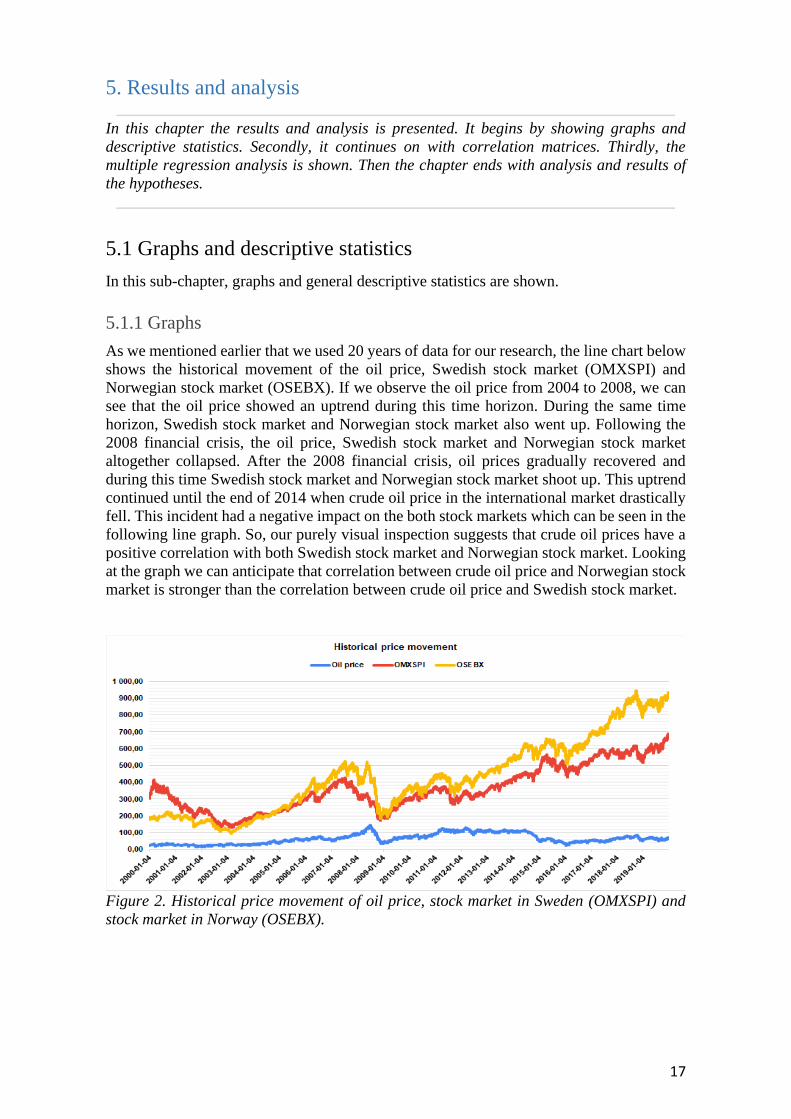
As we mentioned earlier that we used 20 years of data for our research, the line chart below

shows the historical movement of the oil price, Swedish stock market (OMXSPI) and

Norwegian stock market (OSEBX). If we observe the oil price from 2004 to 2008, we can

see that the oil price showed an uptrend during this time horizon. During the same time

horizon, Swedish stock market and Norwegian stock market also went up. Following the

2008 financial crisis, the oil price, Swedish stock market and Norwegian stock market

altogether collapsed. After the 2008 financial crisis, oil prices gradually recovered and

during this time Swedish stock market and Norwegian stock market shoot up. This uptrend

continued until the end of 2014 when crude oil price in the international market drastically

fell. This incident had a negative impact on the both stock markets which can be seen in the

following line graph. So, our purely visual inspection suggests that crude oil prices have a

positive correlation with both Swedish stock market and Norwegian stock market. Looking

at the graph we can anticipate that correlation between crude oil price and Norwegian stock

market is stronger than the correlation between crude oil price and Swedish stock market.

Figure 2. Historical price movement of oil price, stock market in Sweden (OMXSPI) and

stock market in Norway (OSEBX).

18

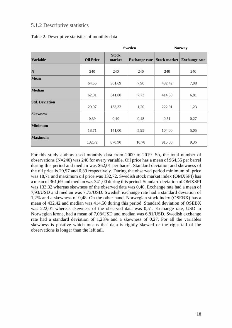
5.1.2 Descriptive statistics

Table 2. Descriptive statistics of monthly data

Sweden Norway

Variable Oil Price

Stock

market Exchange rate Stock market Exchange rate

N 240 240 240 240 240

Mean

64,55 361,69 7,90 432,42 7,08

Median

62,01 341,00 7,73 414,50 6,81

Std. Deviation

29,97 133,32 1,20 222,01 1,23

Skewness

0,39 0,40 0,48 0,51 0,27

Minimum

18,71 141,00 5,95 104,00 5,05

Maximum

132,72 670,90 10,78 915,00 9,36

For this study authors used monthly data from 2000 to 2019. So, the total number of

observations (N=240) was 240 for every variable. Oil price has a mean of $64,55 per barrel

during this period and median was $62,01 per barrel. Standard deviation and skewness of

the oil price is 29,97 and 0,39 respectively. During the observed period minimum oil price

was 18,71 and maximum oil price was 132,72. Swedish stock market index (OMXSPI) has

a mean of 361,69 and median was 341,00 during this period. Standard deviation of OMXSPI

was 133,32 whereas skewness of the observed data was 0,40. Exchange rate had a mean of

7,93/USD and median was 7,73/USD. Swedish exchange rate had a standard deviation of

1,2% and a skewness of 0,48. On the other hand, Norwegian stock index (OSEBX) has a

mean of 432,42 and median was 414,50 during this period. Standard deviation of OSEBX

was 222,01 whereas skewness of the observed data was 0,51. Exchange rate, USD to

Norwegian krone, had a mean of 7,08/USD and median was 6,81/USD. Swedish exchange

rate had a standard deviation of 1,23% and a skewness of 0,27. For all the variables

skewness is positive which means that data is rightly skewed or the right tail of the

observations is longer than the left tail.

19

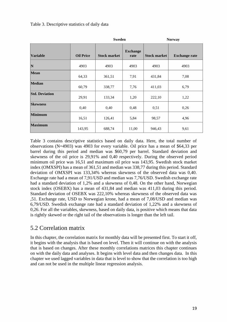
Table 3. Descriptive statistics of daily data

Sweden Norway

Variable Oil Price Stock market

Exchange

rate Stock market Exchange rate

N 4903 4903 4903 4903 4903

Mean 64,33 361,51 7,91 431,84 7,08

Median 60,79 338,77 7,76 411,03 6,79

Std. Deviation 29,91 133,34 1,20 222,10 1,22

Skewness 0,40 0,40 0,48 0,51 0,26

Minimum 16,51 126,41 5,84 98,57 4,96

Maximum 143,95 688,74 11,00 946,43 9,61

Table 3 contains descriptive statistics based on daily data. Here, the total number of

observations (N=4903) was 4903 for every variable. Oil price has a mean of $64,33 per

barrel during this period and median was $60,79 per barrel. Standard deviation and

skewness of the oil price is 29,91% and 0,40 respectively. During the observed period

minimum oil price was 16,51 and maximum oil price was 143,95. Swedish stock market

index (OMXSPI) has a mean of 361,51 and median was 338,77 during this period. Standard

deviation of OMXSPI was 133,34% whereas skewness of the observed data was 0,40.

Exchange rate had a mean of 7,91/USD and median was 7,76/USD. Swedish exchange rate

had a standard deviation of 1,2% and a skewness of 0,48. On the other hand, Norwegian

stock index (OSEBX) has a mean of 431,84 and median was 411,03 during this period.

Standard deviation of OSEBX was 222,10% whereas skewness of the observed data was

,51. Exchange rate, USD to Norwegian krone, had a mean of 7,08/USD and median was

6,79/USD. Swedish exchange rate had a standard deviation of 1,22% and a skewness of

0,26. For all the variables, skewness, based on daily data, is positive which means that data

is rightly skewed or the right tail of the observations is longer than the left tail.

5.2 Correlation matrix

In this chapter, the correlation matrix for monthly data will be presented first. To start it off,

it begins with the analysis that is based on level. Then it will continue on with the analysis

that is based on changes. After these monthly correlations matrices this chapter continues

on with the daily data and analyses. It begins with level data and then changes data. In this

chapter we used lagged variables in data that is level to show that the correlation is too high

and can not be used in the multiple linear regression analysis.

20

5.2.1 Correlation matrix for monthly observations

Table 4. Monthly correlation matrix for data measured by level of the variables

Sweden

Stock

market Oil Price 1 Lag Norway

Stock

market Oil Price 1 Lag

Oil Price ,233** Oil Price ,381**

1 Lag ,994** ,234** 1 Lag ,996** ,382**

Exchange

rate 0,123 -,752** ,129*

Exchange

rate ,189** -,715** ,190**

* 0.1> 0.05 = 10% level ** 0.05> 0.01 = 5% level *** 0.01> = 1% level

Table 4 represents the correlation among the stock market, oil price and other control

variables based on monthly level data. Correlation matrix based on monthly level data

shows that both Swedish and Norwegian stock markets are positively correlated with the

crude oil price. But Norwegian stock market (.381) is more positively correlated with the

oil price compared to the Swedish stock market (.233). For this monthly level data, oil price

to lag correlation is almost equivalent to the stock market to oil price correlation in both

the countries. The lagged variables are perfectly correlated with the current stock market,

so we will not include the lag in the levels regression model. Exchange rate has relatively

low correlation with the stock market in case of Sweden but Norwegian stock market to

Norwegian krone has a correlation of ,189. However, the exchange rate to oil price has a

significantly negative correlation with oil price. Swedish krona to oil price and Norwegian

krone to oil price has a correlation of -,752 and -,715 respectively.

Table 5. Monthly correlation matrix for data measured by changes of the variables

Sweden

Stock

market Oil Price 1 Lag Norway

Stock

market Oil Price 1 Lag

Oil Price ,195** Oil Price ,489**

1 Lag ,268** ,195** 1 Lag ,355** ,322**

Exchange

rate -,179** -,309** -,171**

Exchange

rate -,286** -,449** -,219**

* 0.1> 0.05 = 10% level ** 0.05> 0.01 = 5% level *** 0.01> = 1% level

Table 5 represents the correlation matrix based on monthly changes. Correlation based on

monthly changes also supports our previous results based on monthly level data. Oil price

to the stock market has a positive correlation in both countries. Like the monthly level data,

compared to Swedish stock market, Norwegian stock market to oil price has a higher

positive correlation (.489) based on monthly changes as well. However, authors found a

negative correlation between stock market and exchange rate using monthly changes. Oil

prices and exchange rates still have a negative relation, with a more significant level

compared to monthly level data. Lagged (n=1) effect is also positive in both the countries.

But in case of the stock market and oil price, the lagged (n=1) effect is higher in Norway.

21

5.2.2 Correlation matrix for daily observations

Table 6. Daily correlation matrix for data measured by level of the variables

Sweden

Stock

market Oil Price 1 Lag Norway

Stock

market Oil Price 1 Lag

Oil Price ,235** 1 Oil Price ,381** 1

1 Lag ,999** ,235** 1 1 Lag 1,000** ,382** 1

Exchange

rate ,120** -,748** ,120**

Exchange

rate ,187** -,711** ,187**

* 0.1> 0.05 = 10% level ** 0.05> 0.01 = 5% level *** 0.01> = 1% level

Table 6 represents the correlation matrix based on daily level data. Stock market and oil

price are positively correlated in both countries but Norwegian stock market has higher

positive correlation with oil price based on the daily level data as well. A positive correlation

exists between the stock market and exchange rate. However, exchange rate is significantly

negatively correlated with oil price. In Sweden, Swedish krona to oil price has a correlation

of -,748 and in case of Norway, Norwegian krone to oil price has a correlation of -,711. The

correlation for the lag and the stock market is positive and close to 1 in both countries as

well, so we will not include the lag in the regression model.

Table 7. Daily correlation matrix for Sweden, data measured by changes of the variables

Sweden

Stock

market Oil Price 1 Lag 2 Lag 3 Lag 4 Lag 5 Lag

Oil Price ,205**

1 Lag 0,00 0,01

2 Lag -0,02 0,00 0,00

3 Lag -,040** 0,02 -0,02 0,00

4 Lag 0,00 0,01 -,039** -0,02 -0,01

5 Lag -,036* -0,02 0,00 -,039** -0,02 0,72

Exchange

rate -,121** -,129** -,112** 0,00 0,02 0,02 0,02

* 0.1> 0.05 = 10% level ** 0.05> 0.01 = 5% level *** 0.01> = 1% level

Table 7 represents the correlation matrix based on daily changes data in Sweden. There is a

positive correlation of ,205 between stock price and oil price. Exchange rate changes have

a negative correlation with stock market and oil price changes in Sweden. Lagged (n=5)

stock market changes to oil price changes have a very low correlation but the 5th lag shows

a negative correlation with stock market and oil prices.

22

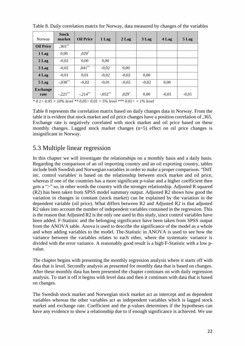
Table 8. Daily correlation matrix for Norway, data measured by changes of the variables

Norway

Stock

market Oil Price 1 Lag 2 Lag 3 Lag 4 Lag 5 Lag

Oil Price ,365**

1 Lag 0,00 ,029*

2 Lag -0,02 0,00 0,00

3 Lag -0,02 ,041** -0,02 0,00

4 Lag -0,01 0,01 -0,02 -0,02 0,00

5 Lag -,038** -0,02 -0,01 -0,02 -0,02 0,00

Exchange

rate -,221** -,214** -,052** ,029* 0,00 -0,01 -0,01

* 0.1> 0.05 = 10% level ** 0.05> 0.01 = 5% level *** 0.01> = 1% level

Table 8 represents the correlation matrix based on daily changes data in Norway. From the

table it is evident that stock market and oil price changes have a position correlation of ,365.

Exchange rate is negatively correlated with stock market and oil price based on these

monthly changes. Lagged stock market changes (n=5) effect on oil price changes is

insignificant in Norway.

5.3 Multiple linear regression

In this chapter we will investigate the relationships on a monthly basis and a daily basis.

Regarding the comparison of an oil importing country and an oil exporting country, tables

include both Swedish and Norwegian variables in order to make a proper comparison. “Diff.

inc. control variables' is based on the relationship between stock market and oil price,

whereas if one of the countries has a more significant p-value and a higher coefficient then

gets a “>” so, in other words the country with the stronger relationship. Adjusted R squared

(R2) has been taken from SPSS model summary output. Adjusted R2 shows how good the

variation in changes in constant (stock market) can be explained by the variation in the

dependent variable (oil price). What differs between R2 and Adjusted R2 is that adjusted

R2 takes into account the number of independent variables contained in the regression. This

is the reason that Adjusted R2 is the only one used in this study, since control variables have

been added. F-Statistic and the belonging significance have been taken from SPSS output

from the ANOVA table. Anova is used to describe the significance of the model as a whole

and when adding variables to the model. The-Statistic in ANOVA is used to see how the

variance between the variables relates to each other, where the systematic variance is

divided with the error variance. A reasonably good result is a high F-Statistic with a low p-

value.

The chapter begins with presenting the monthly regression analysis where it starts off with

data that is level. Secondly analysis as presented for monthly data that is based on changes.

After these monthly data has been presented the chapter continues on with daily regression

analysis. To start it off it begins with level data and then it continues with data that is based

on changes.

The Swedish stock market and Norwegian stock market act as intercept and as dependent

variables whereas the other variables act as independent variables which is lagged stock

market and exchange rate. Coefficient and the p-values determines if the hypotheses can

have any evidence to show a relationship due to if enough significance is achieved. We use

23

a 5 % level of significance in order to find evidence for the hypothesis that a relationship

exists between the variables.

The four regression tables above also include the control variable exchange rate. The

Swedish exchange rate and stock market has a positive relationship on data measured by

level. Data measured by changes resulted in negative relationships and only significant on

the daily basis. Stock markets have a positive relationship to the Norwegian exchange rate

in the results that were measured as level. In contrast the results from the data measured by

changes resulted in negative relationships and only significant on the daily basis.

5.3.1 Multiple linear regression for monthly observations

This chapter shows the regressions for monthly observations where the first one is for level

and second is for changes.

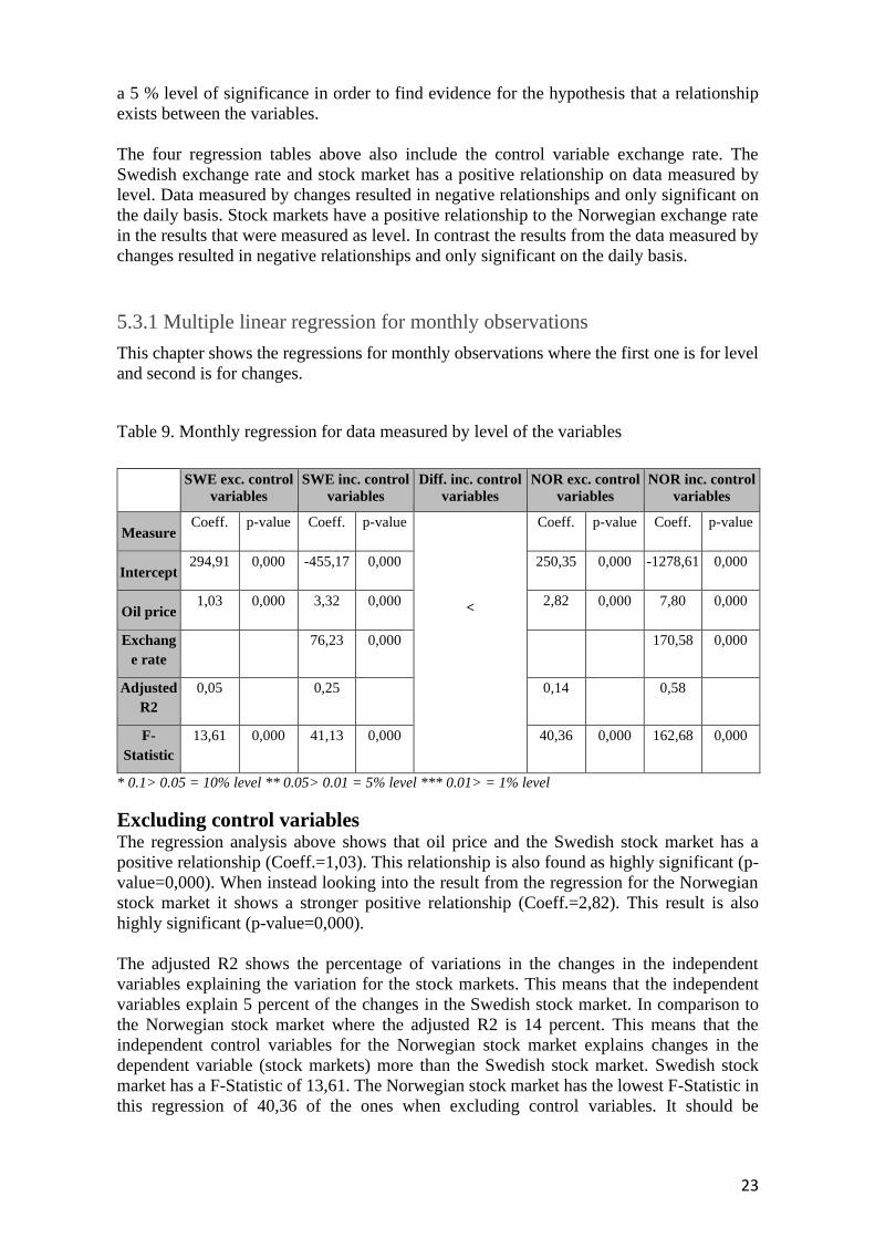
Table 9. Monthly regression for data measured by level of the variables

SWE exc. control

variables SWE inc. control

variables Diff. inc. control

variables NOR exc. control

variables NOR inc. control

variables

Measure Coeff. p-value Coeff. p-value Coeff. p-value Coeff. p-value

Intercept 294,91 0,000 -455,17 0,000 250,35 0,000 -1278,61 0,000

Oil price 1,03 0,000 3,32 0,000

< 2,82 0,000 7,80 0,000

Exchang

e rate

76,23 0,000

170,58 0,000

Adjusted

R2

0,05 0,25

0,14 0,58

F-

Statistic

13,61 0,000 41,13 0,000

40,36 0,000 162,68 0,000

* 0.1> 0.05 = 10% level ** 0.05> 0.01 = 5% level *** 0.01> = 1% level

Excluding control variables The regression analysis above shows that oil price and the Swedish stock market has a

positive relationship (Coeff.=1,03). This relationship is also found as highly significant (p-

value=0,000). When instead looking into the result from the regression for the Norwegian

stock market it shows a stronger positive relationship (Coeff.=2,82). This result is also

highly significant (p-value=0,000).

The adjusted R2 shows the percentage of variations in the changes in the independent

variables explaining the variation for the stock markets. This means that the independent

variables explain 5 percent of the changes in the Swedish stock market. In comparison to

the Norwegian stock market where the adjusted R2 is 14 percent. This means that the

independent control variables for the Norwegian stock market explains changes in the

dependent variable (stock markets) more than the Swedish stock market. Swedish stock

market has a F-Statistic of 13,61. The Norwegian stock market has the lowest F-Statistic in

this regression of 40,36 of the ones when excluding control variables. It should be

24

mentioned that all F-Statistics have the lowest possible significance (p-value=0,000) among

all regressions made, except for one that is mentioned below.

Including control variables The Swedish stock market still holds a positive relationship when including control

variables, which is even stronger than when excluding control variables. (Coeff.=3,32). This

relationship is also found as significant (p-value=0,000). The same pattern is followed by

the Norwegian stock market which has also increased its relationship (Coeff.=7,80). The

same significance level is still achieved in this relationship (p-value=0,000). So, the reason

why the Norwegian stock market achieved a “<” was due to the stronger coefficient since

both stock markets had a significant p-value on the lowest possible level (*** 0.01> = 1%

level) in both excluding control variables and when including control variables. The

regression also shows that the exchange rate has a higher coefficient on the Norwegian stock

market (Coeff.=170,58) than the Swedish stock market (Coeff.=76,23).

The adjusted R2 for the Swedish stock market is 0,25. The Norwegian stock market which

has a higher adjusted R2 of 0,58. This adjusted R2 result for Norway is the highest achieved

adjusted R2 result in the whole study. This is the regression analysis that has the highest

adjusted R2 values as a whole for both Sweden and Norway together. This is exactly the

same explanation as above when excluding control variables, that the independent control

variables for the Norwegian stock market explains changes in the dependent variable (stock

markets) more than the Swedish stock market. Therefore from here on, the adjusted R2

comparison analysis between the Swedish stock market and the Norwegian stock markets

will not be explained as deeply as these. This is because along all regressions, the

Norwegian stock markets have achieved higher adjusted R2 results. F-Statistic for Sweden

was 41,13 and for Norway 162,68 when including control variables.

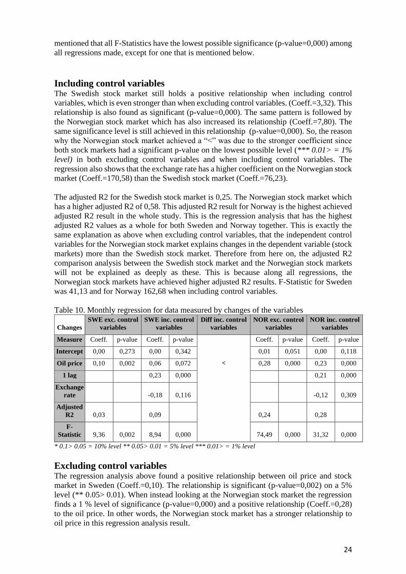
Table 10. Monthly regression for data measured by changes of the variables

Changes

SWE exc. control

variables

SWE inc. control

variables

Diff inc. control

variables

NOR exc. control

variables

NOR inc. control

variables

Measure Coeff. p-value Coeff. p-value

<

Coeff. p-value Coeff. p-value

Intercept 0,00 0,273 0,00 0,342 0,01 0,051 0,00 0,118

Oil price 0,10 0,002 0,06 0,072 0,28 0,000 0,23 0,000

1 lag 0,23 0,000 0,21 0,000

Exchange

rate -0,18 0,116 -0,12 0,309

Adjusted

R2 0,03 0,09 0,24 0,28

F-

Statistic 9,36 0,002 8,94 0,000 74,49 0,000 31,32 0,000

* 0.1> 0.05 = 10% level ** 0.05> 0.01 = 5% level *** 0.01> = 1% level

Excluding control variables The regression analysis above found a positive relationship between oil price and stock

market in Sweden (Coeff.=0,10). The relationship is significant (p-value=0,002) on a 5%

level (** 0.05> 0.01). When instead looking at the Norwegian stock market the regression

finds a 1 % level of significance (p-value=0,000) and a positive relationship (Coeff.=0,28)

to the oil price. In other words, the Norwegian stock market has a stronger relationship to

oil price in this regression analysis result.

25

The adjusted R2 for the Swedish stock market is 0,03 which is the lowest adjusted R2 result

in this study. For the Norwegian stock market it is 0,24 which is the highest adjusted R2

result for Norway when excluding the control variables. For the Swedish stock market this

is the result that indicates the lowest F-Statistic of 9,36. This is also the only F-Statistic that

has a 5% level of significance ** 0.05> 0.01. The significance level of the F-Statistic was

(p-value=0,002). The Norwegian stock market had a F-Statistic of 74,49 with lowest

possible significance exactly as all other F-Statistics.

Including control variables The relationship between the oil price and the Swedish stock market is still positive when

adding control variables in the regression analysis (Coeff.=0,06), though it should be

mentioned that this is a weaker coefficient compared to when excluding control variables.

This relationship is significant (p-value=0,072) but on a 10% level * 0.1> 0.05 . A 10 %

level is not enough significance in order to find evidence for the hypothesis. When instead

looking into the Norwegian stock market, the oil price has a relationship that still is positive

but with a weaker coefficient (Coeff.=0,23). This with the same significance level as when

excluding control variables (p-value=0,000). So, all in all the Norwegian stock market

achieves a “<” since it has higher coefficients and p-values when both excluding and

including control variables.

The lagged variables have similar results where both are significant on 1 % level and the

coefficient for Sweden (Coeff.=0,23) is slightly higher than Norway (Coeff.=0,21).

Exchange rate has a negative relationship for both the Swedish stock market (Coeff.=-0,18)

and the Norwegian stock market (Coeff.=-0,12). Neither of the exchange rates has a

significant level.

The adjusted R2 for the Swedish stock market is 0,09 which compared to the Norwegian

stock market which is 0,28. These regression results show the lowest F-Statistic when

including control variables for both Sweden and for Norway. For Sweden it had a result of

8,94 and for Norway it had a result of 31,32.

5.3.2 Multiple linear regression for daily observations

This chapter shows the regressions for daily observations where the first one is for level and

second is for changes.

Table 11. Daily regression for data measured by level of the variables

Level

SWE exc. control

variables

SWE inc. control

variables

Diff inc. control

variables

NOR exc. control

variables

NOR inc. control

variables

Measure Coeff. p-value Coeff. p-value

<

Coeff. p-value Coeff. p-value

Intercept 294,13 0,000 -439,06 0,000 249,65 0,000 -1258,04 0,000

Oil price 1,05 0,000 3,28 0,000 2,83 0,000 7,73 0,000

Exchange

rate 74,55 0,000 168,32 0,000

Adjusted

R2 0,06 0,25 0,15 0,57

F-

Statistic 286,37 0,000 829,92 0,000 834,62 0,000 3255,22 0,000

* 0.1> 0.05 = 10% level ** 0.05> 0.01 = 5% level *** 0.01> = 1% level

26

Excluding control variables The regression analysis above finds a positive relationship between oil price and the stock

market in Sweden (Coeff.=1,05). This relationship is also significant (p-value=0,000). The

Norwegian stock market also finds a positive relationship (Coeff.=2,83) but with a higher

coefficient than Sweden. This relationship is also significant (p-value=0,000) on the same

level as the Swedish stock market.

Adjusted R2 result for Sweden is 0,06 compared to Norway which has a result of 0,15.

The Swedish stock market had a F-Statistic of 286,37. The F-Statistic in this regression for

the Norwegian stock market is the highest of the ones when excluding control variables.

This F-Statistic was 834,62 for Norway.

Including control variables The Swedish stock market holds the positive relationship when including the control

variables (Coeff.=3,28) which also is significant (p-value=0,000). The Norwegian stock

market is still having a higher coefficient than Sweden when including the variables

(Coeff.=7,73), this relationship is also significant on the same level as Sweden and when

excluding control variables (p-value=0,000). This is the strongest relationship found in this

study when examining the relationship between oil price and stock market. All these

regression analysis for daily level has the lowest possible significance values. So when

comparing Sweden and Norway in the relationship to oil price it can be seen that larger

coefficients are achieved in Norway. This is the reason why the Norwegian stock market

gets a “<” when investigating the difference between the stock markets.

The exchange rate for the Swedish stock market has a positive relationship (Coeff.=74,55)

with a significant result (p-value=0,000). This in comparison to the Norwegian stock market

which has a stronger coefficient (Coeff.=168,32) with the same significance level as the

Swedish stock market.

The adjusted R2 result for Sweden is 0,25 which split the position of scoring the highest

result with “monthly regression measured by level” that also had a result of 0,25. In

comparison to the Norwegian stock market that had an adjusted R2 result of 0,57. The F-

Statistic for Sweden in this result is 829,92. The F-Statistic for the Norwegian stock market

has an extremely high result compared to the other results in this study of 3255,22.

27

Table 12. Daily regression for data measured by changes of the variables

Changes

SWE exc. control

variables

SWE inc. control

variables

Diff inc. control

variables

NOR exc. control

variables

NOR inc. control

variables

Measure Coeff. p-value Coeff. p-value

<

Coeff. p-value Coeff. p-value

Intercept 0,019 0,321 0,023 0,224 0,032 0,087 0,040 0,032

Oil price 0,123 0,000 0,115 0,000 0,227 0,000 0,208 0,000

1 lag -0,019 0,185 -0,022 0,101

2 lag -0,023 0,104 -0,018 0,174

3 lag -0,041 0,003 -0,034 0,010

4 lag -0,006 0,681 -0,018 0,160

5 lag -0,031 0,025 -0,033 0,011

Exchange

rate -0,173 0,000 -0,283 0,000

Adjusted

R2 0,042 0,053 0,133 0,157

F-

Statistic 215,32 0,000 40,36 0,000 753,75 0,000 131,27 0,000

* 0.1> 0.05 = 10% level ** 0.05> 0.01 = 5% level *** 0.01> = 1% level

Excluding control variables The results above show that the Swedish stock market has a positive relationship to oil price

(Coeff.=0,123) with a significant result (p-value=0,000). Compared to the Norwegian stock

market where the coefficient is stronger (Coeff.=0,227) but with the same significance level

(p-value=0,000).

Adjusted R2 result of the Swedish stock market was 0,042 in this regression. For the

Norwegian stock market the result was 0,133 which also is the lowest adjusted R2 result for

Norway in this study when excluding control variables. The F-Statistic in Sweden had a

result of 215,32 and for Norway it had a result of 753,75.

Including control variables This is the part of the study that includes the most control variables since daily observations

and analysis based on changes involved 5 stock market lags. Therefore, the result of this

regression shows that oil price and the Swedish stock market has a positive relationship

(Coeff.=0,115) that is weaker than when excluding control variables. The result is though,

still significant (p-value=0,000). When comparing this to the Norwegian stock market it can

be found that the coefficient have also been reduced (Coeff.=0,208) here when including

control variables. The relationship is still positive with a significant result (p-value=0,000).

Compared to Sweden it is clear that the Norwegian stock market has higher coefficients

when excluding and including control variables, and all results of the relationship between

oil price and stock markets is significant. Therefore, the Norwegian stock market gets the

“<” since it resulted in higher coefficients when comparing the stock markets results.

The lagged variables have negative relationships to the stock markets in both Sweden and

Norway where only some few are significant. The exchange rate relationship to the Swedish

stock market in this regression analysis was negative (Coeff.=-0,173) with significance (p-

value=0,000). The exchange rate for the Norwegian stock market had a relationship to its

stock market that was also negative (Coeff.=-0,283) with a significant result (p-

value=0,000).

28

Adjusted R2 for the Swedish stock market was 0,053 which is the lowest result for Sweden

when including control variables. This compared to the Norwegian stock market who had

an adjusted R2 result of 0,157 which is the lowest result for Norway when including control

variables. The F-Statistic for Sweden was 40,36 and for Norway it was 131,27.

5.3.3 Significance of difference in coefficients

In the separate country regressions analysis, it is clearly evident that coefficient of Norway

is larger than coefficient in Sweden but it can not be said whether the difference is

statistically significant or not. So, we included an interaction between oil price and Swedish

observations and ran a pooled regression including both Sweden and Norway to be sure if

the difference between the coefficients of the two countries is significant or not.

Table 13. Test of difference in coefficients on daily observations

Daily Data Daily changes

exc. control

variables

Daily changes inc.

control variables Daily Level exc.

control variables Daily Level inc.

control variables

Measure Coeff. p-value Coeff. p-value Coeff. p-value Coeff. p-value

Intercept 0,00 0,088 0,00 0,036 249,65 0,000 -1012,83 0,000

OilC 0,23 0,000 0,21 0,000 2,83 0,000 6,94 0,000

Swe 0,00 0,616 0,00 0,549 44,43 0,000 44,47 0,000

OilC*Swe -0,10 0,000 -0,10 0,000 -1,79 0,000 -1,79 0,000

5 Lag -0,03 0,001

4 Lag -0,01 0,211

3 Lag -0,04 0,000

2 Lag -0,02 0,032

1 Lag -0,02 0,028

Exchange Rate -0,23 0,000 140,95 0,000

Adjusted R2 0,09 0,11 0,15 0,58

F-Statistic 321,76 0,000 131,23 0,000 589,90 0,000 3320,69 0,000

**OilC=coefficients in Norwegian sample, **Oil*Swe= interaction coefficient

Table 13 contains coefficients, interaction coefficients, and the respective p-values for the

Swedish and Norwegian observations. According to Martin (2020), “The presence of a

significant interaction indicates that the effect of one predictor variable on the response

variable is different at different values of the other predictor variable.” From Table 13 it is

evident that interaction coefficient is significant based on all sorts of data sets. The

interaction coefficient based on daily level data, including and excluding control variables,

is -1,79 and its corresponding p-value (,000) which is less than ,05. It means that the

interaction coefficient is significant thus the difference between coefficients in Swedish

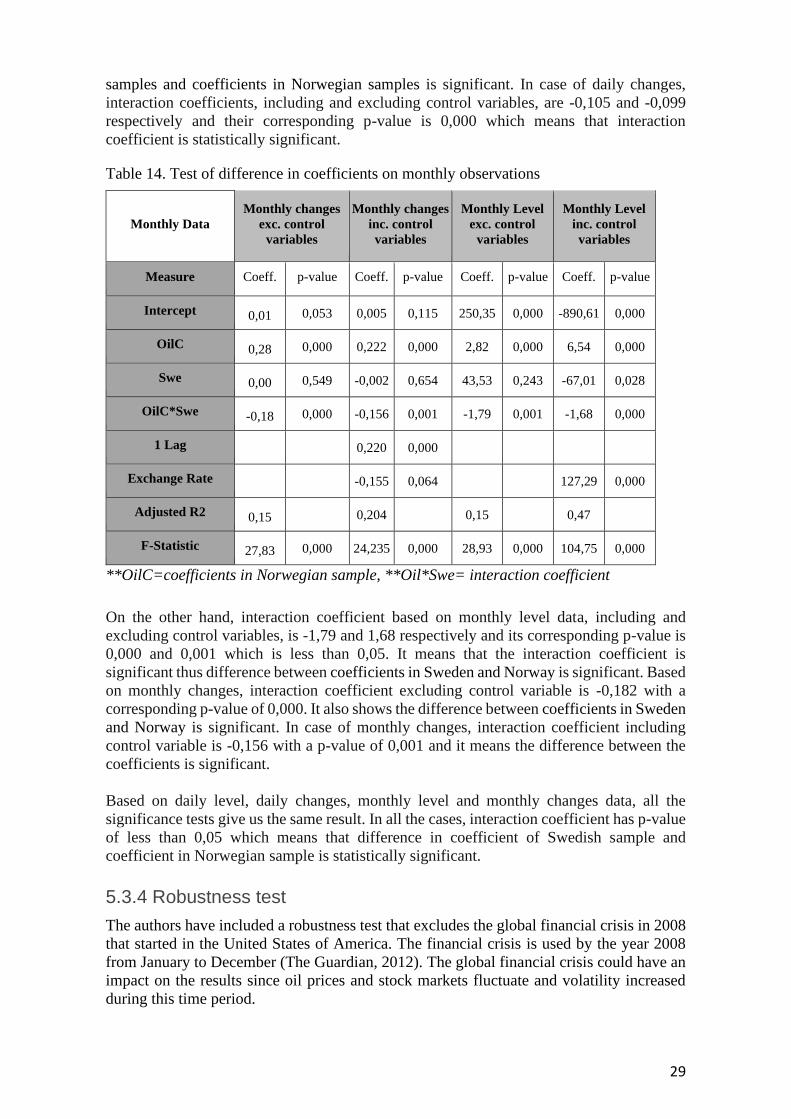
29

samples and coefficients in Norwegian samples is significant. In case of daily changes,

interaction coefficients, including and excluding control variables, are -0,105 and -0,099

respectively and their corresponding p-value is 0,000 which means that interaction

coefficient is statistically significant.

Table 14. Test of difference in coefficients on monthly observations

Monthly Data Monthly changes

exc. control

variables

Monthly changes

inc. control

variables

Monthly Level

exc. control

variables

Monthly Level

inc. control

variables

Measure Coeff. p-value Coeff. p-value Coeff. p-value Coeff. p-value

Intercept 0,01 0,053 0,005 0,115 250,35 0,000 -890,61 0,000

OilC 0,28 0,000 0,222 0,000 2,82 0,000 6,54 0,000

Swe 0,00 0,549 -0,002 0,654 43,53 0,243 -67,01 0,028

OilC*Swe -0,18 0,000 -0,156 0,001 -1,79 0,001 -1,68 0,000

1 Lag 0,220 0,000

Exchange Rate -0,155 0,064 127,29 0,000

Adjusted R2 0,15 0,204 0,15 0,47

F-Statistic 27,83 0,000 24,235 0,000 28,93 0,000 104,75 0,000

**OilC=coefficients in Norwegian sample, **Oil*Swe= interaction coefficient

On the other hand, interaction coefficient based on monthly level data, including and

excluding control variables, is -1,79 and 1,68 respectively and its corresponding p-value is

0,000 and 0,001 which is less than 0,05. It means that the interaction coefficient is

significant thus difference between coefficients in Sweden and Norway is significant. Based

on monthly changes, interaction coefficient excluding control variable is -0,182 with a

corresponding p-value of 0,000. It also shows the difference between coefficients in Sweden

and Norway is significant. In case of monthly changes, interaction coefficient including

control variable is -0,156 with a p-value of 0,001 and it means the difference between the

coefficients is significant.

Based on daily level, daily changes, monthly level and monthly changes data, all the

significance tests give us the same result. In all the cases, interaction coefficient has p-value

of less than 0,05 which means that difference in coefficient of Swedish sample and

coefficient in Norwegian sample is statistically significant.

5.3.4 Robustness test

The authors have included a robustness test that excludes the global financial crisis in 2008

that started in the United States of America. The financial crisis is used by the year 2008

from January to December (The Guardian, 2012). The global financial crisis could have an

impact on the results since oil prices and stock markets fluctuate and volatility increased

during this time period.

30

The results of the (untabulated) robustness test when including the control variables on a

daily basis shows that the significance level of a 1 percent level still holds for all results (p-

value=0,000). Looking at the difference in coefficients when including and excluding year

2008 shows that the Swedish stock market got a weaker relationship (Coeff.=3,28) in the

robustness test than the result in table 11 (Coeff.=3,447) on a level regression. When instead

looking into the Swedish stock market on a regression based on changes the robustness test

showed a weaker relationship (Coeff.=0,102) than in table 12 (Coeff.=0,115). The

Norwegian stock market based on level regression showed a robustness test result of

(Coeff.=7,893) which is stronger than the result in table table 11 (Coeff.=7,73). The same

pattern is followed by the Norwegian stock market where also the regression based on

changes resulted in a higher coefficient when excluding 2008 (Coeff.=0,208) than when

including it (Coeff.=0,181).

So, the result based on data that is level resulted in stronger relationships in the robustness

test than the results in table 11 and table 12. Since the same significance level is achieved

in the robustness tests as in the regressions tables 11 and 12 the comparison of coefficient

was described above. Although the authors could not find any abnormal results in the

robustness tests compared to the regressions in table 11 and 12 since the coefficients are

very close to each other even when excluding year 2008 in the regression.

5.4 Multicollinearity

Besides observing correlations in a correlation matrix to assess multicollinearity concerns,

variance inflation factors (VIF) are assessed r. If there is multicollinearity, it is difficult to

distinguish between the effect that the independent variables actually have on each other

and the effect on the dependent variable. In a multicollinearity test, two different values, a

tolerance value and a variance inflation factor, are analyzed. If multicollinearity does not

occur, the tolerance value should preferably be as high as possible, where the highest value

is 1. The VIF value would preferably be as low as possible, where the lowest value is 1. To

have a relatively approved VIF value, you want it to be below 10. A VIF value above 10

can be directly detrimental to the result since it may contain high degree of multicollinearity

(Yoo et al., 2014).

In general, the Tolerance values for this study is between 0,43 and 1. This as a general aspect

looks reasonably good as a value of 1 is the best possible. The variable that has the lowest

result in VIF and therefore has the lowest possibility of indicating that multicollinearity

exists, is all the lags for Norwegian stock market (VIF=1,00). Instead when looking into the

lowest multicollinearity except for the lagged variables the oil price for Sweden on a daily

basis with changes has the lowest VIF of 1,018. When instead comparing Sweden and

Norway's Tolerance values the authors find that in general Sweden has slightly higher

values, though this is only by a small margin. What the authors of the study did found was

that Tolerance and VIF values for changes become very close to 1 all of them. This is found

as a problem which may occur from using lagged stock market variables. The variable that

has the highest result of indicating that multicollinearity exists (VIF), is oil price (VIF=2,30)

and exchange (VIF=2,30) rate for Sweden on a daily basis with analysis that is level. When

looking at the VIF values as a whole, the lowest was 1 and the highest was 2,30. This is a

similar result as the Tolerance values since one wants to achieve the lowest possible result

close to 1. So, according to Yoo et.al (2014) this is a result that has not caused any problems

since the VIF values are all under 10. In order to look at a more detailed result see appendix

(Table of Multicollinearity).

31

5.5 Analysis

Analyzing the correlation matrices, it is evident that Swedish stock market and Norwegian

stock market both are positively correlated with crude oil price. In case of Sweden,

correlation based on monthly data is in line with correlation based on daily data. We found

a weak positive correlation between crude oil price and Swedish stock market which is in

line with the finding of Zhang and Asche (2014). However, it contradicts theories provided

by Bjørnland (2009) and Fang and You (2014) which we discussed in prior studies.

Bjørnland (2009) and Fang and You (2014) concluded that oil importing countries will have

a negative correlation with the crude oil price. Despite being an oil importing country,

Swedish stock market has a positive correlation with crude oil price which supports Zhang

and Asche (2014). On the other hand Norwegian stock market has a relatively stronger

positive correlation with crude oil price which supports the findings of Zhang and Asche

(2014), Basher et al. (2018) and Bjørnland (2009). Zhang and Asche (2014) concluded that

crude oil price has a stronger positive correlation with Norwegian stock market compared

to Swedish stock market and we also found the same evidence in this study.

All results from the four regression analyses confirm the correlations matrices when looking

into the relationships found. The similarities found by the authors is also that the Norwegian

stock market has a stronger correlation and coefficient than the Swedish stock market when

looking at the relationship to oil price. The positive relationship between the Swedish stock

market and the oil price is not in line with this study's stated hypothesis that was built on

research by Bjørnland (2009) and Fang and You (2014). The reason due to the differences

in the results of their research compared to this study could be that the Swedish stock market

includes industries that not absorbs negative effects when oil price increases and vice versa

(Fang and Egan, 2018).

When comparing the results to the Norwegian stock markets relationship to oil price it can

be found that the research by Hammoudeh and Li (2005), Bjørnland (2009), Basher et al.

(2018) and Zhang and Asche (2014) are in line with the results with this study when

analyzing a oil-exporting country. Since the research by both Hammoudeh and Li (2005)

and Bjørnland (2009) included Norway as their oil-exporting country it is reasonable that

the same result has been found in this study. As mentioned in theory when describing what

causes stock market prices to move, the research by Campbell (1991), shows that fluctuation

depends on crude oil prices. This is what is found in both the Swedish stock market and the

Norwegian stock market. The Norwegian stock market has more evidence than Sweden in

order to support the hypothesis since all the regressions are significant on a 1 % level. So,

since we use a 5 % significance level in order to find evidence that supports the hypothesis

this is something that supports the relationship between the Norwegian stock market and

the oil price, consistent with Hypothesis 2. Since the hypothesis for the Swedish stock

market relationship to the oil price was set as negative and all the regressions showed a

positive relationship, evidence could not be found to support the hypothesis. Although it

was found that the Swedish stock market has a positive significant relationship to oil price

except for one regression on monthly changes when including control variables. So all in

all the Swedish stock market has a positive significant relationship to oil price on a 5 %

significance level except for one regression. Thus, we do not find supportive evidence of

Hypothesis 1, but we are still not able to reject the null of no relationship.

Both the Swedish stock market and the Norwegian stock market have a positive relationship

to the oil price. So, from an investor's point of view a portfolio would benefit as for

diversification effect since the correlations between the stock markets and oil price are

positive but not perfectly correlated (Baur and Lucey, 2010). If having the Swedish stock

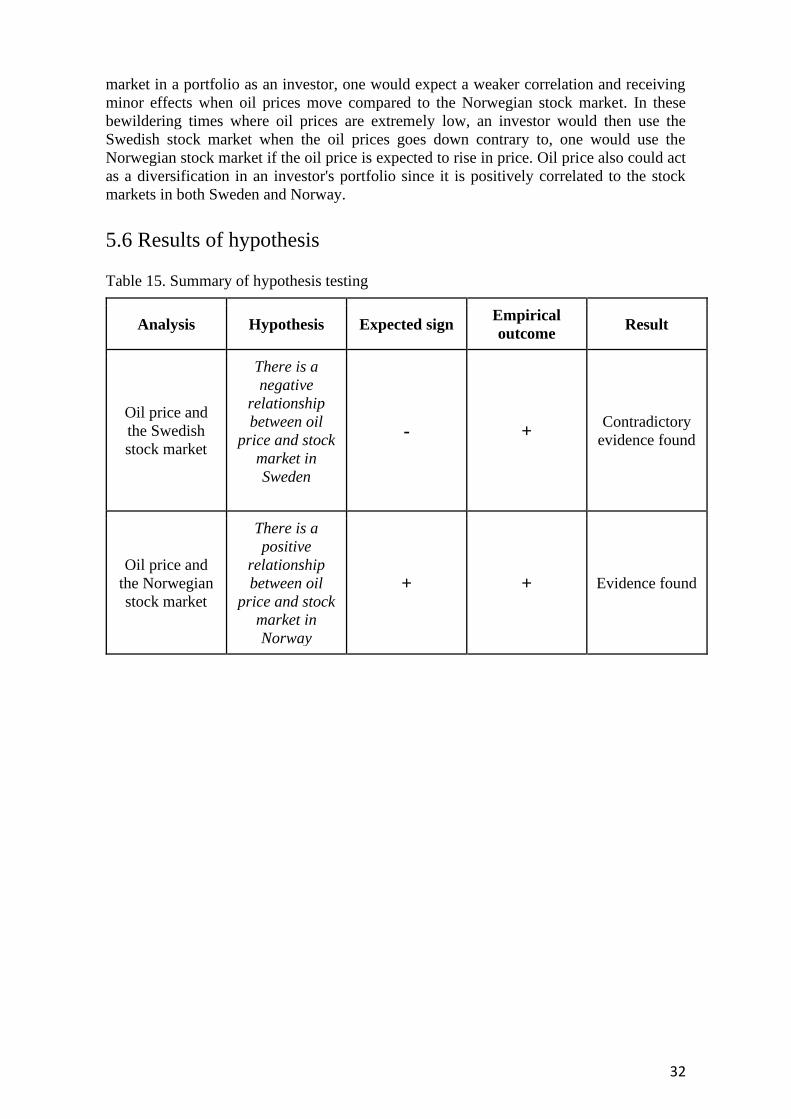
32

market in a portfolio as an investor, one would expect a weaker correlation and receiving

minor effects when oil prices move compared to the Norwegian stock market. In these

bewildering times where oil prices are extremely low, an investor would then use the

Swedish stock market when the oil prices goes down contrary to, one would use the

Norwegian stock market if the oil price is expected to rise in price. Oil price also could act

as a diversification in an investor's portfolio since it is positively correlated to the stock

markets in both Sweden and Norway.

5.6 Results of hypothesis

Table 15. Summary of hypothesis testing

Analysis Hypothesis Expected sign Empirical

outcome Result

Oil price and

the Swedish

stock market

There is a

negative

relationship

between oil

price and stock

market in

Sweden

- + Contradictory

evidence found

Oil price and

the Norwegian

stock market

There is a

positive

relationship

between oil

price and stock

market in

Norway

+ + Evidence found

33

6. Conclusion and proposal for future studies

This chapter presents a conclusion of the study. Where the results and study´s contribution

of the research area will be presented. After that the proposal for future studies will be

discussed.

6.1 Conclusion

The main purpose of this study was to examine the relationship of crude oil price with

Swedish stock market and Norwegian stock market. It also explores the exchange rate and

lagged stock market relationship to the stock markets in Sweden and Norway. Here, authors

used a linear regression model to examine the relationship between crude oil price and stock

market. Using the linear regression model and correlation matrix, authors found that

Swedish stock market and Norwegian stock market have a positive relationship with crude

oil price.

So, this paper supports the hypothesis that there is a positive relationship between oil price

and stock market in Norway as there has been evidence found in this research. In Norwegian

economy, an increase in oil price has a stimulating impact on the stock market which is

consistent with the prior studies on oil exporting countries. This result is in line with

previous researchers such as Hammoudeh and Li (2005), Bjørnland (2009), Basher et al.

(2018) and Zhang and Asche (2014). However, no evidence has been found on the

hypothesis that there is a negative relationship between oil price and stock market in

Sweden. Instead we found a positive correlation between crude oil price and Swedish stock

market in this study which contradicts Bjørnland (2009) and Fang and You (2014) but this

result is supported by Zhang and Asche (2014). Bjørnland (2009) and Fang and You (2014)

concluded that oil importing countries have a negative relation with crude oil price. Despite

being an oil importing country, Sweden has a positive relation with crude oil price. Main

reason behind this can be market integration in the Nordic region. In a general aspect, the

relationships still stay the same as for significance level and coefficients in the robustness

test made. One contribution of this study is that investors can use oil price in order to create

a diversification effect in their portfolios in both the Swedish and the Norwegian stock

market.

We used the exchange rate which is a macro economic factor, as an independent control

variable. The estimates showed that there is a strong negative correlation between exchange

rates (Swedish krona and Norwegian krone) and crude oil price in both of the countries. So,

Swedish krona and Norwegian krone depreciates when oil price goes up and vice versa. We

also conducted a significance test to determine if the interaction in the regression is

significant or not. We found that the difference in coefficient of Swedish sample and

coefficient in Norwegian sample is statistically significant. Finally, this study contributes to

the research in the Nordic region. Only a few studies can be found in this region, specially

in Sweden. Hence, this study will enrich the research works on this region.

6.2 Limitations and proposal for future studies

In the last decade, the Nordic region has experienced some financial reforms. As a matter

of fact, markets are becoming more integrated day by day. Market integration in this region

can be one of the main reasons behind the positive correlation with Swedish stock market

34

and crude oil price. We suggest to examine the market integration of this region to look at

how much one country influences another. We would also suggest to analyze the fact that

to what extent the effects on the stock market depends on the different reasons behind the

oil price changes. Lastly, our study was focused on oil importing and exporting countries in

the Nordic region. We would like to suggest to examine the other stock market indices from

other parts of the world and see if the relation between oil price and stock market is the

same as it is in this region. While conducting this research, we could not avoid some issues.

These issues are the main limitations of this study. One limitation of this study is that authors

explored only one macroeconomic factor among many. The authors tried to figure out the

impact of oil price change on the exchange rate. But there are other important

macroeconomic factors such as interest rate, inflation rate etc., which are extremely vital

for every economy. The authors could not cover those macroeconomic factors in this study.

Therefore, the proposal for future studies is that future researchers can include other

macroeconomic factors such as inflation interest rate etc. and see the co movement of the

factors.

6.3 Generalizability

The generalizability of this study is based on how well the research can be generalized in

different research and different markets. This is in other words a discussion of how well the

research findings can be redone in other circumstances which also relies on validity

(Saunders et al., 2009). We think that the generalizability of our findings is at least for the

Norwegian stock market assure since prior studies have found the same relationships. In the

contrary, the Swedish stock market which was very new in this research area, found a

relationship that is not the most usual in oil-importing countries. Therefore, we think that in

general this finding may not be good in a generalizability aspect. But in similar economies

and in the same region (Nordic countries) it may be good. Our study is based on long series

of data and well known methods which is good for the generalizability according to us.

35

References

Arbnor, I., and Bjerke, Bjorn. (1994). Foretagsekonomisk Metodlara.

Areal, N., Oliveira, B., and Sampaio, R. (2013). When times get tough, gold is golden.

The European Journal of Finance, 1-20.

Apergis, Nicholas, Miller, Stephen M., (2009). Do structural oil-market shocks affect

stock prices? Energy Economics 31, 569–575.

Basher, S. A., Haug, A. A., and Sadorsky, P. (2018). The impact of oil-market shocks on

stock returns in major oil-exporting countries. Journal of International Money and

Finance, 86, 264–280.

Barsky, Robert, Kilian, Lutz, (2004). Oil and macroeconomy since the 1970s. Journal of

Economic Perspectives 18, 115–134.

Baur, D and Lucey, B. (2010). Is Gold a Hedge or a Safe Haven? An Analysis of Stocks,

Bonds and Gold. Financial Review, 45( 2), 217-229.

Bastianin, A., Conti, F., and Manera, M. (2016). The impacts of oil price shocks on stock

market volatility: Evidence from the G7 countries. Energy Policy, 98, 160–169.

Bjørnland, H. C. (2009). Oil price shocks and stock market booms in an oil exporting

country. Scottish Journal of Political Economy, 56(2), 232–254.

Bjørnland, H. C. (2000). The dynamic effects of aggregate demand, supply and oil

price shocks - a comparative study. The Manchester School of Economic Studies, 68, pp.

578–607.

Bohi, D. R. (1989). Energy Price Shocks and Macroeconomic Performance. Washington:

Resources for the Future.

Burbidge, J. and HARRISON, A. (1984). Testing for the effects of oil-price rises using

vector auto regressions. International Economic Review, 25, pp. 459–84.

Carollo, S. (2012). Understanding oil prices : a guide to what drives the price of oil in

today's markets. Hoboken, N.J.: Hoboken, N.J. : Wiley.

Carrington, D., Ambrose, J. and Taylor, M. (2020). Will the coronavirus kill the oil

industry and help save the climate? The Guardian. Available via:

https://www.theguardian.com/environment/2020/apr/01/the-fossil-fuel-industry-is-broken-

will-a-cleaner-climate-be-the-result (2020-05-13)

Caplinger, D. (2020). What Is a Stock Market Index? The Motley Fool. Available via:

https://www.fool.com/knowledge-center/what-is-a-stock-index.aspx (Retrieved 2020-05-

11)

Chen, J. (2020). What Is Crude Oil? Investopedia. Available via:

https://www.investopedia.com/terms/c/crude-oil.asp (Retrieved 2020-05-15)

36

Chen, S.-S. (2010). Do higher oil prices push the stock market into bear territory? Energy

Economics, 32(2), 490–495.

Cong RG, Wei YM, Jiao JL et al. (2008) Relationships between oil price shocks and stock

market: An empirical analysis from China. Energy Policy, 36, 3544–3553.

Cuñado, J. Perez De Gracia, F. (2003). Do oil price shocks matter? Evidence from some

European countries. Energy Economics, 25, pp. 137–54.

David, D., (2020). Coronavirus: Oil price collapses to lowest level for 18 years. BBC

News. https://www.bbc.com/news/business-52089127 [Retrieved 2020-05-05]

Demirbas, A., Omar Al-Sasi, B., and Nizami, A.-S. (2017). Recent volatility in the price

of crude oil. Energy Sources, Part B: Economics, Planning, and Policy, 12(5), 408–414.

Energy Information Administration. (2020a). Petroleum & other liquids. Available via:

https://www.eia.gov/dnav/pet/hist/rbrteD.htm. (Retrieved 2020-03-30)

Energy Information Administration. (2020b). Information Quality Guidelines. Available

via: https://www.eia.gov/about/information_quality_guidelines.php. (Retrieved 2020-04-

14)

Fang, C., and You, S. (2014). The impact of oil price shocks on the large emerging

countries’ stock prices: Evidence from China, India and Russia. International Review of

Economics and Finance, 29, 330–338.

Filis, G., Degiannakis, S., and Floros, C. (2011). Dynamic correlation between stock

market and oil prices: The case of oil-importing and oil-exporting countries. International

Review of Financial Analysis, 20(3), 152–164.

Fang, S., Lu, X., and Egan, P. G. (2018). Reinvestigating the Oil Price–Stock Market

Nexus: Evidence from Chinese Industry Stock Returns. China & World Economy, 26(3),

43–62.

Fawley, B.W., Juvenal, L. and Petrella, I. (2012). When Oil Prices Jump, Is Speculation

To Blame? Federal Reserve Bank of St. Louis. Available via:

https://www.stlouisfed.org/publications/regional-economist/april-2012/when-oil-prices-

jump-is-speculation-to

blame#:~:text=Higher%20oil%20prices%20require%20that,dollar%20increase%20in%20

oil%20prices.&text=Speculative%20demand%20can%20and%20did,bust%20cycle%20in

%20commodity%20prices. (Retrieved 2020-06-10)

Geske, R., and Roll, R. (1983). The Fiscal and Monetary Linkage between Stock Returns

and Inflation. Journal of Finance 38: 1–33.

Hamilton, J. (2009). Understanding Crude Oil Prices. The Energy Journal, 30(2), 179–

206.

Hammoudeh, S., & Li, H. (2005). Oil sensitivity and systematic risk in oil-sensitive stock

indices. Journal of Economics and Business, 57(1), 1–21.

Hazem Marashdeh, and Akhsyim Afandi. (2017). Oil Price Shocks and Stock Market

Returns in the Three Largest Oil-producing Countries. International Journal of Energy

Economics and Policy, 7(5), 312–322.

37

JodiOil, (2019). JODI Oil World Database. Available via: https://www.jodidata.org/oil/

(retrieved 2020-05-12)

Kilian, Lutz, (2008). Exogenous oil supply shocks: how big are they and how much do

they matter for the US economy? Review of Economics and Statistics 90, 216–240.

Kilian, L. (2009). Not All Oil Price Shocks Are Alike: Disentangling Demand and Supply

Shocks in the Crude Oil Market. American Economic Review, 99(3), 1053–1069.

Kilian, Lutz, (2009). Not all oil price shocks are alike: disentangling demand and supply

shocks in the crude oil market. American Economic Review 99, 1053–1069.

Kilian, Lutz, Park, Cheolbeom, 2009. The impact of oil price shocks on the US stock

market. International Economic Review 50, 1267–1287.

Kim, K. (2003). Dollar exchange rate and stock price: Evidence from multivariate

cointegration and error correction model. Review of Financial Economics, 12(3), 301-313.

Miyazaki, T., and Hamori, S. (2013). Testing for causality between the gold return and

stock market performance: Evidence for ‘gold investment in case of emergency’. Applied

Financial Economics, 23(1), 27-40.

Guru-Gharana, K K, Rahman, M and Parayitam S, (2009),’Influence of

SelectedMacroeconomic Variables on U.S Stock Market Returns and their Predictability

over Varying Time Horizons’, Academy of Accounting and Financial Studies Journal,

13(1), s.1-19

Haldane, A. G. (1997). The monetary framework in Norway. In A. B. Christiansen and J.

F. Qvigstad (eds.), Choosing a Monetary Policy Target. Oslo: Scandinavian University

Press, pp. 67–108.

Hamilton, James D., (1983). Oil and the macroeconomy since World War II. Journal of

Political Economy 91, 228–248.

Hamilton, James D., (1996). This is what happened to the oil price-macroeconomy

relationship. Journal of Monetary Economics 38, 215–220.

Hamilton, James D., (2003). What is an oil shock? Journal of Econometrics 113, 363–

398.

Hooker, Mark A., (1996). What happened to the oil price-macroeconomy relationship?

Journal of Monetary Economics 38, 195–213.

Höglund, H. and Sundvik, D., (2019). Do auditors constrain intertemporal income shifting

in private companies? Accounting and Business Research, 49(3), 245-270

LEE, K., NI, S. and RATTI, R. A. (1995). Oil shocks and the macroeconomy: the role of

price variability. Energy Journal, 16, pp. 39–56.

Li, S.-F., Zhu, H.-M. and Yu, K. (2012) Oil prices and stock market in China: A sector

analysis using panel cointegration with multiple breaks, Energy Economics, 34, 1951–8.

38

Li, X., and Liu, Yuan Chun. (2011). Analysis of influencing factors of international oil

price fluctuations. ProQuest Dissertations Publishing. Retrieved from

http://search.proquest.com/docview/1874969161/

Louis, R. J., and Balli, F. (2014). Oil Price and Stock Market Synchronization in Gulf

Cooperation Council Countries. Emerging Markets Finance and Trade, 50(1), 22–51.

Martin, K. J. (2020). Interpreting Interactions in Regression. The Analysis Factor.

https://www.theanalysisfactor.com/interpreting-interactions-in-regression/ [Retrieved

2020-05-04]

Macrotrends (2020). Crude Oil Prices - 70 Year Historical Chart. Macrotrends.

https://www.macrotrends.net/1369/crude-oil-price-history-chart [Retrieved 2020-04-15]

Melike E. Bildirici, and Mesut M. Badur. (2018). The effects of oil prices on confidence

and stock return in China, India and Russia. Quantitative Finance and Economics, 2(4),

884–903.

Moberg, K. (2015-03-03). Ar artikeln peer reviewed?. Karolinska institutet.

https://kib.ki.se/whatsup/blog/ar-artikeln-peer-reviewed. (Retrieved: 2020-03-31)

Mork, K. A. (1989). Oil and the macroeconomy when prices go up and down: an

extension of Hamilton's results. Journal of Political Economy, 91, pp. 740–4.

Mork, K. A., OLSEN, Ø. and MYSEN, H. T. (1994). Macroeconomic responses to oil

price

increases and decreases in seven OECD countries. Energy Journal, 15, pp. 19–35.

Muhammad, Z., Suleiman, H., and Kouhy, R. (2012). Exploring oil price—exchange rate

nexus for Nigeria. OPEC Energy Review, 36(4), 383–395.

Narayan, P.K., Narayan, S. (2010), Modeling the impact of oil prices on Vietnam’s stock

prices. Apply Energy, 87, 356-361.

Nasdaq. (2020a). OMXSPI. OMX STOCKHOLM PI. Available via:

http://www.nasdaqomxnordic.com/indexes/historical_prices?Instrument=SE0000744195.

(Retrieved 2020-03-30)

Nasdaq. (2020b). Om oss. Available via: http://www.nasdaqomxnordic.com/omoss.

(Retrieved 2020-04-14)

Nath Sahu, T., Bandopadhyay, K., and Mondal, D. (2014). An empirical study on the

dynamic relationship between oil prices and Indian stock market. Managerial Finance,

40(2), 200–215.

Norges Bank. (2020a). USD/NOK. Available via: https://www.norges-

bank.no/tema/Statistikk/Valutakurser/?tab=currency&id=USD. (Retrieved 2020-04-07)

Norges Bank. (2020b). Om Banken. Available via: https://www.norges-bank.no/tema/Om-

Norges-Bank/ . (Retrieved 2020-04-07)

Nwosa, P. I. (2014). Oil prices and stock market price in Nigeria. OPEC Energy Review,

38(1), 59–74.

39

Organization of the Petroleum Exporting Countries (2020). Member Countries. Available

via: https://www.opec.org/opec_web/en/about_us/25.htm (Retrieved 2020-06-07)

Oslo Børs. (2020a).The history in words and pictures. Available via:

https://www.oslobors.no/anniversary. (Retrieved: 2020-03-29)

Oslo Børs. (2020b). OSEBX. Hovedindeksen. Available via:

https://www.oslobors.no/markedsaktivitet/#/details/OSEBX.OSE/overview. (Retrieved:

2020-04-06)

Oslo Børs. (2020c). Om Oslo Børs. Available via: https://www.oslobors.no/Oslo-

Boers/Om-Oslo-Boersv. (Retrieved: 2020-04-06)

Oskooe, S. A. P. (2012). Oil price shocks and stock market in oil‐exporting countries:

evidence from Iran stock market. OPEC Energy Review, 36(4), 396–412.

Park, Jungwook, Ratti, Ronald A., (2008). Oil price shocks and stock markets in the US

and 13 European countries. Energy Economics 30, 2587–2608.

Radetzki, M. (2012). Politics—not OPEC interventions—explain oil's extraordinary price

history. Energy Policy, 46, 382–385.

R.A. Badeeb, H.H. Lean. (2018). Asymmetric impact of oil price on Islamic sectoral

stocks. Energy Economics, 71 , pp. 128-139

Riksbanken. (2020a). USD/SEK. Available via: https://www.riksbank.se/sv/statistik/sok-

rantor--valutakurser/?g130-SEKUSDPMI=on&from=1999-01-29&to=2020-01-

02&f=Month&c=cAverage&s=Comma. (Retrieved 2020-04-07)

Riksbanken. (2020b). Om Riksbanken. Available via: https://www.riksbank.se/sv/om-

riksbanken/ . (Retrieved 2020-04-07)

Sadorsky, P. (1999). Oil price shocks and stock market activity. Energy Economics, 21, 5,

pp. 449–69.

Sadorsky, P., (2001). Risk factors in stock returns of Canadian oil and gas companies.

Energy Econ. 23 (1), 17–28.

Saunders, M., Lewis, P. & Thornhill, A. 2009. Research Methods for Business. 5th

edition. England: Pearson Education Limited.

Garside, M. (2019). OPEC - Statistics & Facts. Statista. Available via:

https://www.statista.com/topics/1830/opec/ (Retrieved 2020-06-08)

The Guardian. (2012). Financial crisis. timeline. Available via:

https://www.theguardian.com/business/2012/aug/07/credit-crunch-boom-bust-timeline

(Retrieved 2020-05-12)

Times, T. E. (2020). Definition of 'Stock Market'. The Economic Times.

https://economictimes.indiatimes.com/definition/stock-market (Retrieved 2020-05-11)

Wang, Y., Wu, C., and Yang, L. (2013). Oil price shocks and stock market activities:

Evidence from oil-importing and oil-exporting countries. Journal of Comparative

Economics, 41(4), 1220–1239.

40

Workman, D. (2020). Crude Oil Imports by Country. World's Top Exports. Available via:

http://www.worldstopexports.com/crude-oil-imports-by-country/ [Retrieved: 2020-05-19]

Yoo, W., Mayberry, R., Bae, S., Singh, K., Peter He, Q., and Lillard, J. (2014). A Study of

Effects of MultiCollinearity in the Multivariable Analysis. International Journal of

Applied Science and Technology, 4(5), 9-19.

Zhang, D, Asche, F. (2014) The oil price shocks and Nordic stock markets. Int. J. of Trade

and Global Markets, 7(4), 300–315.

Zhu, H., Guo, Y., and You, W. (2015). An empirical research of crude oil price changes

and stock market in China: evidence from the structural breaks and quantile regression.

Applied Economics, 47(56), 6055–6074.

Zhang H., Wei J. and Huang J. (2014). Scaling and Predictability in Stock Markets: A

Comparative Study. Plos One 9(3), e91707.

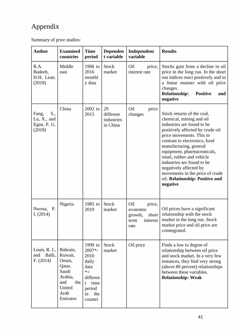
41

Appendix

Summary of prior studies:

Author Examined

countries

Time

period

Dependen

t variable

Independent

variable

Results

R.A.

Badeeb,

H.H. Lean.

(2018)

Middle

east

1996 to

2016

monthl

y data

Stock

market

Oil price,

interest rate

Stocks gain from a decline in oil

price in the long run. In the short

run indices react positively and in

a linear manner with oil price

changes.

Relationship: Positive and

negative

Fang, S.,

Lu, X., and

Egan, P. G.

(2018)

China 2002 to

2015

29

different

industries

in China

Oil price

changes Stock returns of the coal,

chemical, mining and oil

industries are found to be

positively affected by crude oil

price movements. This in

contrast to electronics, food

manufacturing, general

equipment, pharmaceuticals,

retail, rubber and vehicle

industries are found to be

negatively affected by

movements in the price of crude

oil. Relationship: Positive and

negative

Nwosa, P.

I. (2014)

Nigeria 1985 to

2010

Stock

market

Oil price,

economic

growth, short

term interest

rate

Oil prices have a significant

relationship with the stock

market in the long run. Stock

market price and oil price are

cointegrated.

Louis, R. J.,

and Balli,

F. (2014)

Bahrain,

Kuwait,

Oman,

Qatar,

Saudi

Arabia,

and the

United

Arab

Emirates

1999 to

2007*-

2010

daily

data

*=

differen

t time

period

in the

countri

Stock

market

Oil price Finds a low to degree of

relationship between oil price

and stock market. In a very few

instances, they find very strong

(above 80 percent) relationships

between these variables.

Relationship: Weak

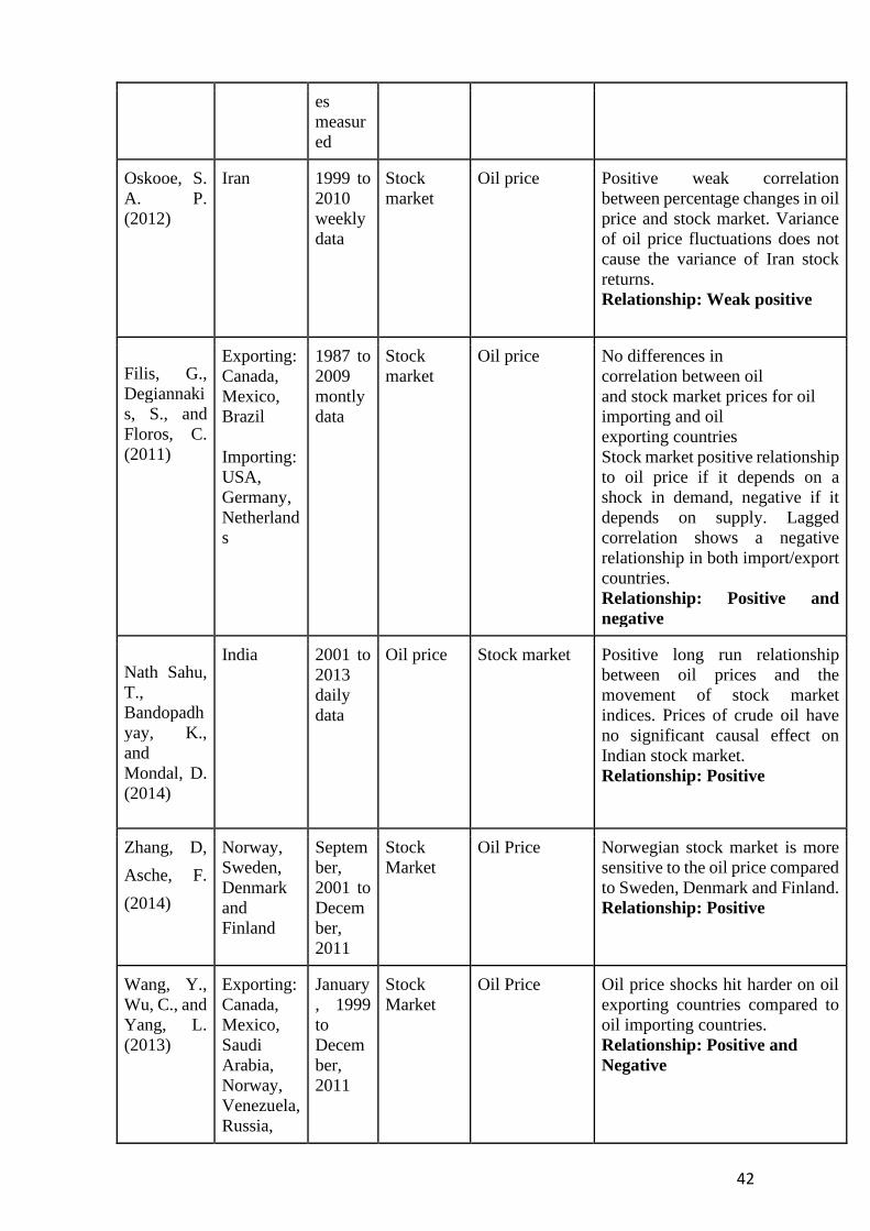
42

es

measur

ed

Oskooe, S.

A. P.

(2012)

Iran 1999 to

2010

weekly

data

Stock

market

Oil price Positive weak correlation

between percentage changes in oil

price and stock market. Variance

of oil price fluctuations does not

cause the variance of Iran stock

returns.

Relationship: Weak positive

Filis, G.,

Degiannaki

s, S., and

Floros, C.

(2011)

Exporting:

Canada,

Mexico,

Brazil

Importing:

USA,

Germany,

Netherland

s

1987 to

2009

montly

data

Stock

market

Oil price No differences in

correlation between oil

and stock market prices for oil

importing and oil

exporting countries

Stock market positive relationship

to oil price if it depends on a

shock in demand, negative if it

depends on supply. Lagged

correlation shows a negative

relationship in both import/export

countries.

Relationship: Positive and

negative

Nath Sahu,

T.,

Bandopadh

yay, K.,

and

Mondal, D.

(2014)

India 2001 to

2013

daily

data

Oil price Stock market Positive long run relationship

between oil prices and the

movement of stock market

indices. Prices of crude oil have

no significant causal effect on

Indian stock market.

Relationship: Positive

Zhang, D,

Asche, F.

(2014)

Norway,

Sweden,

Denmark

and

Finland

Septem

ber,

2001 to

Decem

ber,

2011

Stock

Market

Oil Price Norwegian stock market is more

sensitive to the oil price compared

to Sweden, Denmark and Finland.

Relationship: Positive

Wang, Y.,

Wu, C., and

Yang, L.

(2013)

Exporting:

Canada,

Mexico,

Saudi

Arabia,

Norway,

Venezuela,

Russia,

January

, 1999

to

Decem

ber,

2011

Stock

Market

Oil Price Oil price shocks hit harder on oil

exporting countries compared to

oil importing countries.

Relationship: Positive and

Negative

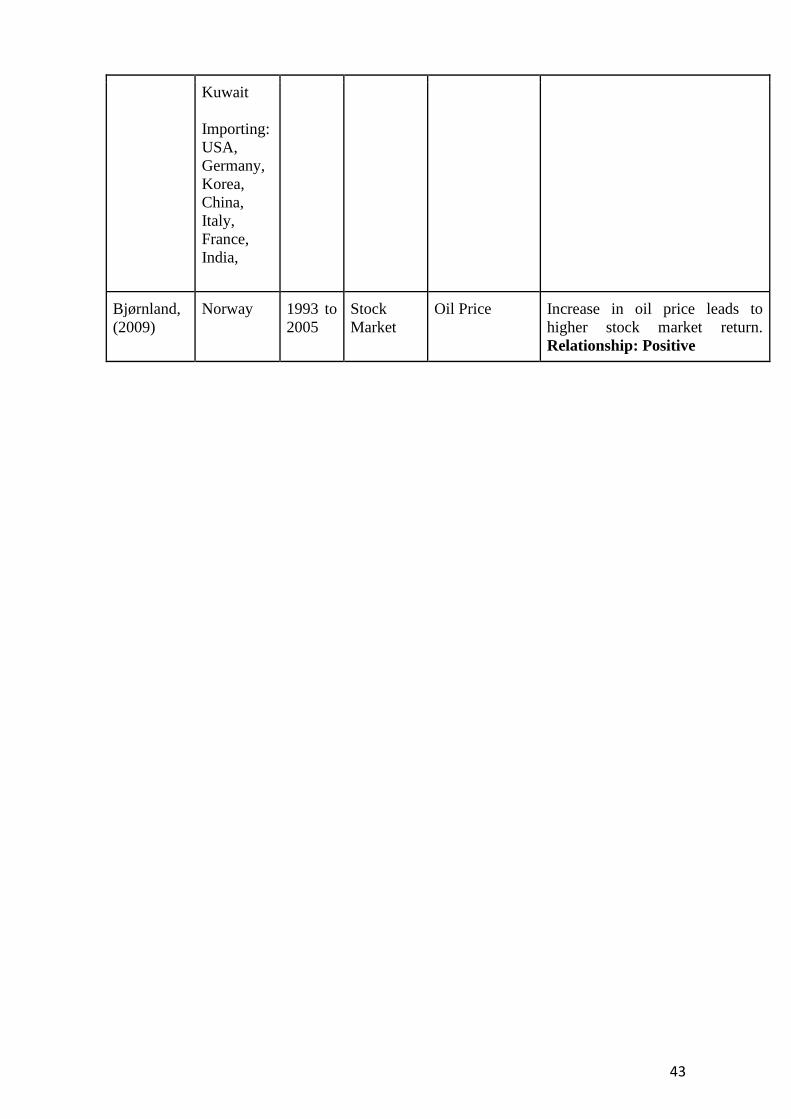
43

Kuwait

Importing:

USA,

Germany,

Korea,

China,

Italy,

France,

India,

Bjørnland,

(2009)

Norway 1993 to

2005

Stock

Market

Oil Price Increase in oil price leads to

higher stock market return.

Relationship: Positive

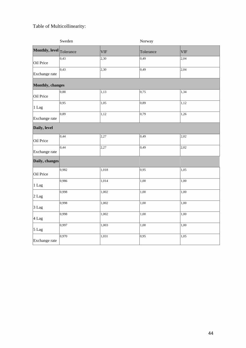
44

Table of Multicollinearity:

Sweden Norway

Monthly, level Tolerance VIF Tolerance VIF

Oil Price 0,43 2,30 0,49 2,04

Exchange rate 0,43 2,30 0,49 2,04

Monthly, changes

Oil Price 0,88 1,13 0,75 1,34

1 Lag 0,95 1,05 0,89 1,12

Exchange rate 0,89 1,12 0,79 1,26

Daily, level

Oil Price 0,44 2,27 0,49 2,02

Exchange rate 0,44 2,27 0,49 2,02

Daily, changes

Oil Price 0,982 1,018 0,95 1,05

1 Lag 0,986 1,014 1,00 1,00

2 Lag 0,998 1,002 1,00 1,00

3 Lag 0,998 1,002 1,00 1,00

4 Lag 0,998 1,002 1,00 1,00

5 Lag 0,997 1,003 1,00 1,00

Exchange rate 0,970 1,031 0,95 1,05

45

Business Administration SE-901 87 Umeå www.usbe.umu.se