The relation between Acid Volatile Sulfides (AVS) and metal accumulation in aquatic invertebrates: Implications of feeding behavior and ecology

lable at ScienceDirect

Environmental Pollution 158 (2010) 1381–1391

Contents lists avai

Environmental Pollution

journal homepage: www.elsevier .com/locate/envpol

The relation between Acid Volatile Sulfides (AVS) and metal accumulation inaquatic invertebrates: Implications of feeding behavior and ecology

Maarten De Jonge*, Ronny Blust, Lieven BervoetsDepartment of Biology, Ecophysiology, Biochemistry and Toxicology Group, University of Antwerp, Groenenborgerlaan 171, B-2020 Antwerp, Belgium

The relation between AVS and metal accumulation in aquatic inverteb

a r t i c l e i n f o

Article history:Received 22 October 2009Received in revised form28 December 2009Accepted 7 January 2010

Keywords:AVSMacro-invertebratesBioaccumulationExposure routes

* Corresponding author. Tel.: þ32 3 265 3533; fax:E-mail address: [email protected] (M. De

0269-7491/$ – see front matter � 2010 Elsevier Ltd.doi:10.1016/j.envpol.2010.01.001

a b s t r a c t

The present study evaluates the relationship between Acid Volatile Sulfides (AVS) and metal accumu-lation in invertebrates with different feeding behavior and ecological preferences. Natural sediments,pore water and surface water, together with benthic and epibenthic invertebrates were sampled at 28Flemish lowland rivers. Different metals as well as metal binding sediment characteristics including AVSwere measured and multiple regression was used to study their relationship with accumulated metals inthe invertebrates taxa.

Bioaccumulation in the benthic taxa was primarily influenced by total metal concentrations in thesediment. Regarding the epibenthic taxa metal accumulation was mostly explained by the morebioavailable metal fractions in both the sediment and the water. AVS concentrations were generallybetter correlated with metal accumulation in the epibenthic invertebrates, rather than with the benthictaxa. Our results indicated that the relation between AVS and metal accumulation in aquatic inverte-brates is highly dependent on feeding behavior and ecology.

� 2010 Elsevier Ltd. All rights reserved.

1. Introduction

Metal accumulation in aquatic organisms is very complex anddepends on different exposure routes (overlying water, pore water,food and sediment) and environmental influences on bioavail-ability in both water and sediment (Luoma and Rainbow, 2005). Inthe oxic boundary layer of natural sediments, trace elements aremainly associated with sedimentary phases such as organic matter,clay content and iron, manganese and aluminum oxides (Luoma,1983; Bervoets et al., 1997, 2005). In anoxic sediments one of themost important factors controlling metal availability are the AcidVolatile Sulfides (AVS). AVS is operationally defined as the amountof sulfides volatilized by the addition of 1 N HCl and is mainlyconsisting of iron and manganese sulfides (Di Toro et al., 1990,1992). The metals which are associated with AVS are calledSimultaneously Extracted Metals (SEM). SEM is generally deter-mined as the metal fraction which describes the sum of molarconcentrations of toxicologically important, cationic metals (Cu, Pb,Cd, Zn and Ni) which are extracted together with AVS (Di Toro et al.,1992). Furthermore also Cr (Berry et al., 2004) and Ag (Yoo et al.,2004) can be associated with AVS. From this, Di Toro et al. (1990)

þ32 3 265 3497.Jonge).

All rights reserved.

formulated the SEM–AVS model for metal sediment toxicity. Thismodel predicts that when AVS concentrations in sediments, ona molar basis, exceed SEM concentrations (SEM–AVS < 0), allmetals will be bound to sulfides and the sediment pore water isconsidered to be non-toxic. On the opposite, when the sedimentcontains an excess of SEM (SEM–AVS > 0), metals will be releasedinto the sediment pore water and become potentially toxic to theaquatic life (Di Toro et al., 1990, 1992).

The SEM–AVS model has been validated for both acute (e.g. DiToro et al., 1990) and chronic toxicity (Hare et al., 1994; Ingersollet al., 1994). However, the relation between AVS and metal accu-mulation is not yet fully understood. During the last years, signifi-cant evidence has been gained that benthic invertebrates canaccumulate metals, even when [SEM–AVS] < 0; This as well duringlaboratory experiments (Hare et al., 1994; Ingersoll et al., 1994; Leeet al., 2000a,b, 2001; Yoo et al., 2004) as under natural fieldconditions (De Jonge et al., 2009). These results can be explained bythe fact that benthic invertebrates, which live most of the time inthe sediment, ingest sediment particles as their main food source,regardless of AVS (Lee et al., 2000a,b; De Jonge et al., 2009). Asconditions within animal guts can differ substantially from sedi-mentary environments, metal availability can be modified drasti-cally. This will finally result in an enhanced bioaccumulation(Griscom et al., 2000, 2002). Since the preceding studies almostonly assessed bioaccumulation in benthic invertebrates, it is not

M. De Jonge et al. / Environmental Pollution 158 (2010) 1381–13911382

obvious that the same assumptions can be made for other inver-tebrates, which do not reside most of the time in the sediment butinhabit the overlying surface water. This because the relativeimportance of metal exposure routes (overlying water, pore water,food and sediment) is likely to depend on the feeding behavior andecological preferences of animals (Warren et al., 1998). Therefore itis important to consider these biological characteristics as wellwhen studying the relation between AVS and metal accumulation.

The main objective of the present study was to evaluate therelationship between [SEM–AVS] and metal accumulation ininvertebrates with different feeding behavior and ecologicalpreferences. This was done by assessing AVS and other importantmetal binding characteristics in sediments of different Flemishlowland rivers and relate these characteristics to metal concen-trations found in several invertebrate taxa. We hypothesized thatinvertebrate species, living most of the time in the surface water(epibenthic taxa), are more exposed to metal concentrations in thewater (mainly through the Free metal Ion), which leaches out viathe sediment pore water. Therefore it is likely that metal accu-mulation in epibenthic taxa is correlated with [SEM–AVS]. This incontrast with sediment inhabiting taxa (benthic), which ingest thebulk sediment and as a result accumulate metals primarily fromthe sediment, regardless of AVS or other metal bindingcharacteristics.

2. Material and methods

2.1. Study area and sampling design

In total 28 sampling sites were chosen, based on measurements performed bythe Flemish Environment Agency (see database available from www.vmm.be, 2009,Flemish Environmental Association: water monitoring data bank, Belgium) andresults from former studies (Bervoets et al., 1997, 2005; Bervoets and Blust, 2003; DeJonge et al., 2009) (Table 1). All samples were taken in the spring of 2008.

At every sampling site, pH, temperature, dissolved oxygen and ElectricalConductivity (EC) of the surface water were measured in-situ using a HachHQ30d Multi-Parameter field kit; each time 3 water samples were collected forthe analysis of trace metals, major cations and Dissolved Organic Carbon (DOC).

Table 1Location and coordinates of the different sampling sites.

Site River Basin Location XY-Coordinates

1 Eindergatloop Dommel/Meuse Neerpelt 223398 2143672 Dommel Meuse Neerpelt 223907 2135683 Dommel Meuse Neerpelt 223523 2145124 Dommel Meuse Neerpelt 223533 2173955 Dommel Meuse Neerpelt 223950 2180806 Kneutersloop Nete/Scheldt Olen 185353 2089637 Asbeek Nete/Scheldt Balen 210621 2028128 Desselse Nete Nete/Scheldt Dessel 199929 2155829 Molse Nete Nete/Scheldt Mol 211498 20906710 Asbeek Nete/Scheldt Olmen 210621 20281211 Diepteloop Nete/Scheldt Beerse 179427 21411812 Kleine Nete Nete/Scheldt Dessel 199000 21456013 Scheppelijke Nete Nete/Scheldt Mol 203131 20930514 Scheppelijke Nete Nete/Scheldt Mol 208591 21083015 Zwarte beek Demer/Scheldt Beringen 207810 19132016 Visbeddebeek Nete/Scheldt Leopoldsburg 208625 20383917 Molse Nete Nete/Scheldt Mol 206536 20831318 Molse Nete Nete/Scheldt Mol 201657 20770919 Diepteloop Nete/Scheldt Beerse 179430 21412420 Diepteloop Nete/Scheldt Beerse 180661 22268021 Rijt Dender/Scheldt Ninove 124728 16891822 Kruisbeek Dender/Scheldt Ternat 131472 17492923 Moerbeek Scheldt Nazareth 101249 18380724 Molenbeek Scheldt Puurs 144568 19683325 Fabrieksloop Nete/Scheldt Willebroek 150165 19513726 Bankloop Nete/Scheldt Olen 187070 20910927 Dalloop Nete/Scheldt Beerse 181778 22299028 Laakbeek Nete/Scheldt Beerse 181637 222337

Also 3 field blanks were transported to the field in order to detect possiblecontamination while taking and transporting the samples. All samples werestored in 20 ml acid-washed polypropylene vials at 4 �C until analysis. Thesediment top layer (0–2 cm) was sampled manually in triplicates. At the lab, thesamples were immediately frozen at �20 �C, which is the recommended storingprocedure to maintain AVS concentrations within the sampled sediment (deLange et al., 2008).

Invertebrate samples were taken with a pondnet (500 mm mesh, 200 � 300 mmframe and 500 mm bag depth) fitted to a 1.5 m handle. The collected invertebrateswere depurated by placing them for 24 h in artificial OECD (Organization ofEconomic Cooperation and Development) water (2 mM CaCl2.2H2O, 500 mMMgSO4.7H2O, 771 mM NaHCO3 and 77.1 mM KCl). The samples were dried for at least24 h at 60 �C. Subsequently, the biological material was digested with concentratedultrapure nitric acid (96% HNO3) in a microwave (Blust et al., 1988) and stored untilanalysis.

The different invertebrates analyzed for metal content were identified asChironomus gr. thummi, a benthic species complex living and feeding on thesediment (Hare and Campbell, 1992), Tubifex sp., a benthic Oligochaete (Pennak,1989); Asellus aquaticus and Physa acuta, two epibenthic invertebrates mostlyfeeding on algae (van Hattum et al., 1989; Goodyear and McNeill, 1999); Erpobdellaoctoculata, a freshwater leech feeding on Chironomus gr. thummi and A. aquaticus(Goodyear and McNeill, 1999; Kutschera, 2003) and the predating stonefly larvaeIsoperla grammatica, which also feeds on Chironomus gr. thummi (Elliott, 2004)(Table 1). At each site 3 till 6 replicates of the collected invertebrate taxa wereanalyzed (Table 2).

2.2. Water and sediment characterization

Dissolved Organic Carbon content (DOC) in the water samples was measuredusing a Total Organic Carbon Analyzer (TOC-5000/5050, Shimadzu Corporation,Kyoto, Japan). In order to get a general image of the water hardness, Ca and Mgconcentrations were measured together with the trace metals (see 2.3).Regarding the sediment samples, a subsample of each sediment was centrifugedat 10 000 g using a 5804 R Eppendorf centrifuge (Eppendorf AG, Hamburg,Germany) in order to collect pore water (PW) (Ankley and Schubauer-Berigan,1994). The supernatant was decanted and filtered through a 0.22 mm membranefilter and acidified with concentrated HNO3 (69%; Merck, Germany). Acid VolatileSulfides were extracted from wet sediment using the modified diffusion methodof Leonard et al. (1996); the extracted amount of sulfides was measured with anORION 96-16 ion-selective sulphur electrode (Ionplus, Beverly, MA, USA). After-wards the wet/dry ratio of the sediment sample was determined in order toconvert the measured sulfide value to dry weight. The remaining SEM fractionwas stored in a fridge at 4 �C until metal analysis. The organic matter content ofthe sediment was determined through Loss of Ignition (LOI). For this purpose drysediment was incinerated at 550 �C for 4 h. In order to quantify the sediment’sclay content, it’s particle-size distribution was analyzed via laser diffraction(Malvern Mastersizer S., Worcestershire, UK) (Queralt et al., 1999). The total metalcontent was measured by drying the sediments at 60 �C for 48 h and addinga mixture of HNO3 (69%) and HCl (37%)(1:3, v/v); subsequently, samples weretransferred to Teflon� bombs and digested in a microwave oven (ETHOS 900Microwave Labstation, Milestone, Italy) (Tessier et al., 1984). After digestion,samples were filtered and diluted with ultrapure water (MilliQ�, Bedford, MA,USA) up to 50 ml and stored until metal analysis.

2.3. Metal analysis and chemical speciation

Trace metals (As, Cd, Co, Ag, Cr, Cu, Zn, Ni and Pb) and other important cations(Al, Ca, Na, K, Fe, Mn and Mg) were measured in total surface water and in samplesfiltered through a 0.2 mm cellulose acetate filter (Schleicher & Schuell MicroScienceGmbH, Dassel, Germany). Particulate bound metals (PaSW) in the surface waterwere calculated by subtracting the dissolved metal concentrations from the totalmetal concentrations. Trace metals together with Al, Fe and Mn were measured inpore water (also filtered through a 0.22 mm membrane), sediment (Total as well asSEM) and invertebrate samples. Together with the trace metals Al, Fe and Mn, whichare known to form oxyhydroxide precipitates and regulate the metal concentrationin the sediment (Davis and Leckie, 1978), were measured in the extracted SEMfraction. All metal analysis were performed using an Inductively Coupled PlasmaMass Spectrometer (ICP-MS, Varian UlatraMass 700, Victoria, Australia), withGermanium (Ge) as internal standard. Analytical accuracy was achieved by the useof blanks and certified reference material (CRM) of the Community Bureau ofReference (European Union, Brussels, Belgium) during all the above-mentioneddestruction protocols, including standards for trace elements in river sediment(CRM 320) and mussel tissue (CRM 278). Recoveries were within 10% of the certifiedvalues.

The Free metal Ion Activity (FIA) of the different trace metals in the surface waterwas calculated using the Windermere Humic Aqueous Model version 6 softwarepackage (WHAM 6; Natural Environment Research Council, Swindon, UK) (Tipping,1998). This model utilizes the Humic Ion-Binding Model VI for the calculations ofion-binding by humic matter. Concentrations of the cations (Al, Ca, Na, K, Fe, Mn and

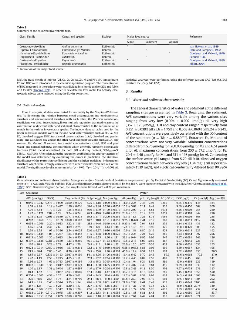
Table 2Summary of the collected invertebrate taxa.

Class–Family Genus and species Ecology Major food source Reference

Algae Sediment Animal

Crustaceae–Asellidae Asellus aquaticus Epibenthic * van Hattum et al., 1989Diptera–Chironomidae Chironomus gr. thummi Benthic * Hare and Campbell, 1992Hirudinea–Erpobdellidae Erpobdella octoculata Epibenthic * Goodyear and McNeill, 1999Oligochaeta–Tubificidae Tubifex sp. Benthic * Pennak, 1989Gastropoda–Physidae Physa acuta Epibenthic * Goodyear and McNeill, 1999Plecoptera–Perlodiddae Isoperla grammatica Epibenthic * Elliott, 2004

*: Indication of the major food source.

M. De Jonge et al. / Environmental Pollution 158 (2010) 1381–1391 1383

Mg), the trace metals of interest (Cd, Co, Cr, Cu, As, Zn, Ni and Pb), pH, temperature,EC and DOC were introduced in the chemical speciation program. The concentrationof DOC measured in the surface water was divided into humic acid for 20% and fulvicacid for 80% (Tipping, 1998). In order to calculate the Free metal Ion Activity, elec-trostatic effects were included using the Davies correction.

2.4. Statistical analysis

Prior to analysis, all data were tested for normality by the Shapiro–Wilkinsontest. To determine the relation between metal accumulation and environmentalvariables and environmental variables with each other, the Pearson correlation-coefficient was used. Subsequently, linear multiple regression was used to assess thecontribution of different water and sediment characteristics to the accumulation ofmetals in the various invertebrate species. The independent variables used for thelinear regression models were on the one hand water variables such as pH, Ca, Mg,EC, dissolved oxygen, DOC, trace metal concentrations (total, dissolved and partic-ulate) and calculated FIA, and on the other hand sediment variables such as LOI, claycontent, Fe, Mn and Al content, trace metal concentrations (total, SEM and porewater) and normalized metal concentrations which generally represent bioavailablefractions (Total metal normalized for both LOI and clay content, SEMMe–AVS,SEMMe–AVS/LOI). After calculating the regression coefficients the appropriateness ofthe model was determined by examining the errors in prediction, the statisticalsignificance of the regression coefficients and the variation explained. Independentvariables which were strongly correlated with other variables were left out of themodel. The significance level is represented as *p< 0.05; **p< 0.01; ***p< 0.001. All

Table 3General water and sediment characteristics. Average values (n ¼ 3) and standard deviationonce (n¼ 1). AVS: Acid Volatile Sulfides; LOI: Loss of Ignition (Organic Matter content); Fe1996); DOC: Dissolved Organic Carbon, the samples were filtered with a 0.22 mm memb

Site Sediment

AVS (mmol/g) LOI (%) Clay content (%) Fe (mmol/g) Mn (mmol/g) Al

1 0.045 � 0.042 0.476 � 0.099 0.600 � 0.170 5.75 � 1.18 0.099 � 0.017 112 2.09 � 2.98 1.12 � 0.447 1.56 � 0.036 68.6 � 3.86 0.296 � 0.057 153 4.01 � 5.64 1.70 � 1.22 1.15 � 0.515 56.0 � 13.9 0.199 � 0.010 134 1.22 � 0.171 2.04 � 1.29 9.24 � 6.24 76.3 � 49.6 0.440 � 0.278 235 1.18 � 1.05 0.801 � 0.589 0.777 � 0.275 39.2 � 27.1 0.200 � 0.256 136 0.292 � 0.460 1.19 � 0.169 0.850 � 0.182 48.7 � 10.0 0.191 � 0.053 9.77 0.054 � 0.066 2.20 � 0.933 3.22 � 1.15 282 � 44.6 0.549 � 0.113 9.38 1.65 � 2.54 2.43 � 2.69 3.89 � 2.75 189 � 123 1.44 � 1.48 179 6.59 � 2.55 1.05 � 0.336 2.54 � 0.025 52.0 � 6.27 0.036 � 0.008 1010 0.556 � 0.135 1.08 � 0.257 1.84 � 0.352 51.5 � 13.8 0.099 � 0.026 1411 0.013 � 0.003 1.30 � 0.623 1.34 � 0.530 25.9 � 6.55 1.96 � 1.81 3912 0.197 � 0.138 0.981 � 0.589 1.23 � 0.250 46.1 � 5.77 0.123 � 0.040 1013 120 � 70.5 3.28 � 2.74 4.47 � 1.70 245 � 119 1.40 � 1.52 2314 0.024 � 0.014 0.450 � 0.036 1.67 � 0.211 72.2 � 11.6 0.040 � 0.006 6.515 29.5 � 36.4 7.80 � 5.45 8.76 � 6.59 245 � 55.6 1.26 � 0.597 4516 1.85 � 2.57 0.836 � 0.163 0.937 � 0.159 14.1 � 4.96 0.106 � 0.080 1617 2.42 � 1.19 2.58 � 0.245 4.05 � 1.11 253 � 57.2 0.234 � 0.100 1418 7.96 � 6.23 1.62 � 0.733 0.947 � 0.195 142 � 18.2 0.345 � 0.043 1019 0.047 � 0.040 1.35 � 0.817 0.877 � 0.123 10.4 � 1.00 0.605 � 0.190 2320 4.10 � 2.83 1.38 � 0.644 1.47 � 0.493 41.6 � 17.0 0.264 � 0.309 1521 10.4 � 1.42 1.19 � 0.057 0.503 � 0.060 47.4 � 8.18 4.47 � 0.742 3622 0.204 � 0.065 4.57 � 2.25 4.79 � 3.61 95.4 � 24.5 20.4 � 4.46 1923 226 � 88.6 25.6 � 1.75 3.74 � 0.700 244 � 68.4 11.0 � 3.00 8324 14.3 � 3.85 2.40 � 0.544 5.75 � 1.54 28.6 � 7.08 0.801 � 0.226 2125 357 � 125 19.9 � 8.23 5.20 � 1.17 227 � 57.6 4.35 � 2.01 3126 0.004 � 0.002 0.828 � 0.512 3.36 � 1.26 42.6 � 8.59 0.052 � 0.011 6.527 0.063 � 0.044 0.710 � 0.075 1.43 � 0.307 11.2 � 2.53 0.111 � 0.056 1228 0.045 � 0.053 0.351 � 0.039 0.810 � 0.260 26.6 � 3.10 0.120 � 0.061 9.5

statistical analyses were performed using the software package SAS (SAS 9.2, SASInstitute Inc., Cary, NC, USA).

3. Results

3.1. Water and sediment characteristics

The general characteristics of water and sediment at the differentsampling sites are presented in Table 3. Regarding the sediment,AVS concentrations were very variable among the various sitesranging from very low (0.004 � 0.002 mmol/g) till very high(357 � 125 mmol/g). LOI and clay content ranged respectively from0.351�0.039% till 25.6�1.75% and 0.503� 0.060% till 9.24� 6.24%.AVS concentrations were positively correlated with the LOI contentof the sediment (n ¼ 38; r ¼ 0.889***). Extracted Fe, Mn and Alconcentrations were not very variable. Minimum concentrationsdiffered from 5.75 mmol/g for Fe, 0.036 mmol/g for Mg and 6.51 mmol/g for Al; maximum concentrations from 253 � 57.2 mmol/g for Fe,20.4 � 4.46 mmol/g for Mn and 311 �198 mmol/g for Al. Concerningthe surface water, pH ranged from 5.70 till 9.10, dissolved oxygenconcentrations varied between very low (3.34 mg/l) till supersatu-rated (11.19 mg/l), and electrical conductivity differed from 80.9 mS/

s are presented; pH, O2, Electrical Conductivity (EC), Ca and Mg were only measured, Mn and Al were together extracted with the SEM after HCl extraction (Leonard et al.,rane.

Water

(mmol/g) pH O2 (mg/l) EC (mS/cm) DOC (mg/l) Ca (mmol/l) Mg (mmol/l)

.0 � 2.24 7.35 7.98 3260 9.65 � 0.316 1135 184

.2 � 5.07 7.11 9.48 335 9.09 � 0.450 562 209

.9 � 2.00 7.12 8.81 1031 9.26 � 0.008 755 210

.6 � 10.6 7.19 8.75 1057 8.42 � 0.303 842 216

.1 � 11.6 7.23 8.76 1066 9.26 � 0.008 868 2255 � 0.478 7.41 7.15 762 6.00 � 0.013 2112 2163 � 1.05 7.04 8.88 234 8.14 � 0.132 433 122.1 � 10.6 9.10 9.96 326 15.8 � 0.329 608 155.9 � 1.81 6.80 10.19 628 5.09 � 0.013 1225 192.7 � 2.28 7.24 8.25 280 7.34 � 0.054 997 256.1 � 9.44 6.95 9.96 546 9.97 � 0.081 743 126.5 � 2.15 6.97 10.56 367 6.07 � 0.041 726 161.9 � 15.0 6.70 10.35 438 4.50 � 0.031 1036 1938 � 0.652 6.83 9.96 499 4.40 � 0.057 1124 195.9 � 12.4 6.57 8.22 197 9.02 � 0.062 336 76.3.4 � 6.42 5.70 9.45 80.9 15.6 � 0.068 77.5 37.0.2 � 4.40 6.82 7.55 408 7.52 � 6.45 768 141.4 � 1.04 6.24 8.62 394 15.0 � 0.468 625 119.2 � 4.02 7.49 9.81 416 9.29 � 0.183 639 112.8 � 2.49 6.18 8.50 302 9.57 � 0.038 539 113.7 � 4.18 8.16 10.58 785 5.15 � 0.218 1856 550.7 � 3.61 8.34 9.95 614 34.3 � 0.184 1606 389.8 � 27.0 7.97 11.19 603 10.5 � 0.041 1904 202.0 � 2.96 8.41 7.43 835 6.13 � 0.043 2160 4881 � 198 7.45 3.34 2370 16.9 � 0.364 2078 3491 � 1.74 6.97 5.26 4810 7.89 � 0.087 237 72.4.5 � 1.88 6.81 8.48 392 13.2 � 0.059 233 53.72 � 7.61 6.42 4.84 310 6.47 � 0.027 671 102

M. De Jonge et al. / Environmental Pollution 158 (2010) 1381–13911384

cm till 5810 mS/cm. DOC concentrations showed little variation,ranging from 4.40� 0.057 mg/l till 34.3� 0.184 mg/l; Ca ranged from77.5 mmol/l till 2112 mmol/l and Mg from 37.0 mmol/l till 550 mmol/l.Ca and Mg concentrations were positively correlated (n ¼ 38;r¼ 0.773***). Ca was positively correlated (n¼ 38; r¼ 0.603***) withpH as well; dissolved oxygen in the surface water was negativelycorrelated with AVS concentrations in the sediment (r ¼ �0.494**).

3.2. Metal concentrations in the environment

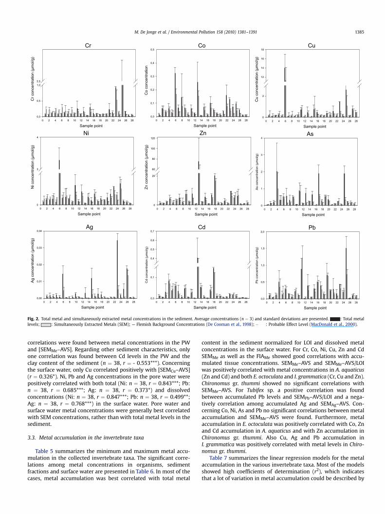
Fig. 1 presents the total (ToSW), dissolved (DiSW) as well asparticulate (PaSW) metal concentrations and Free metal IonActivities (FIA) in the surface water. At most sites dissolved metalconcentrations were rather high with maximum values of1.62 � 0.075 mmol/l for Cr; 2.75 � 0.214 mmol/l for Co;1.61 � 0.224 mmol/l for Ni; 6.74 � 0.962 mmol/l for Cu;47.5 � 4.33 mmol/l for Zn; 0.416 � 0.065 mmol/l for As; 1.31710�3 � 0.114 10�3 mmol/l for Ag; 0.127 � 0.016 mmol/l for Cd and0.235� 0.583 mmol/l for Pb. Except for sampling point 26, 27 and 28dissolved metal concentrations were generally higher than partic-ulate bound metals. Regarding the calculated Free metal Ion

Cr

Sample point

Cr c

once

ntra

tion

(µm

ol/l)

Ni

Sample point

Ni c

once

ntra

tion

(µm

ol/l)

Ag

Sample point

Ag c

once

ntra

tion

(µm

ol/l)

C

Sa

Co

conc

entra

tion

(µm

ol/l)

Z

Sam

Zn c

once

ntra

tion

(µm

ol/l)

C

Sa

Cd

conc

entra

tion

(µm

ol/l)

Fig. 1. Dissolved metal concentrations and free metal ion activity in the surface water. Withdeviations are presented. Regarding the free ion activity only one value was calculated. ADissolved metal levels; : Particulate metal levels; : Free metal ion activity; — —: FFramework directive criteria (Nixon and Zabel, 2005).

Activities (FIA) of the different metals in the surface water, veryhigh values were found for Cu (0.931 mmol/l), Zn (7.89 mmol/l), Cd(0.212 mmol/l) and Pb (0.672 mmol/l). The FIA of Cu was positivelycorrelated with [SEMCu–AVS] (n ¼ 38; r ¼ 0.333*).

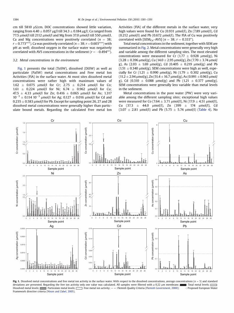
Total metal concentrations in the sediment, together with SEM aresummarized in Fig. 2. Metal concentrations were generally very highand variable among the different sampling sites. The most elevatedconcentrations were measured for Cr (1.77 � 0.928 mmol/g), Ni(3.28� 0.396 mmol/g), Cu (14.0� 2.95 mmol/g), Zn (7.70� 3.74 mmol/g), As (2.03 � 1.69 mmol/g), Cd (0.405 � 0.219 mmol/g) and Pb(1.51 � 0.340 mmol/g). SEM concentrations were high as well, espe-cially for Cr (1.21 � 0.990 mmol/g), Ni (1.79 � 0.302 mmol/g), Cu(11.2� 2.94 mmol/g), Zn (51.4�16.7 mmol/g), As (0.991�0.963 mmol/g), Cd (0.310 � 0.088 mmol/g) and Pb (1.21 � 0.377 mmol/g).SEM concentrations were generally less variable than metal levelsin the sediment.

Metal concentrations in the pore water (PW) were very vari-able among the different sampling sites; exceptional high valueswere measured for Co (7.64 � 3.71 mmol/l), Ni (17.9 � 4.51 mmol/l),Cu (37.3 � 44.0 mmol/l), Zn (399 � 174 mmol/l), Cd(3.07 � 2.81 mmol/l) and Pb (5.75 � 5.74 mmol/l) (Table 4). No

o

mple point

n

ple point

d

mple point

Cu

Sample point

Cu

conc

entra

tion

(µm

ol/l)

As

Sample point

As c

once

ntra

tion

(µm

ol/l)

Pb

Sample point

Pb c

once

ntra

tion

(µm

ol/l)

respect to the dissolved concentrations, average concentrations (n ¼ 3) and standardll samples were filtered with a 0.22 mm membrane. : Total metal levels; :lemish Quality Criteria (Flemish Government, 2000); : Proposed European Water

Cr

Sample point0 2 4 6 8 10 12 14 16 18 20 22 24 26 28

Cr c

once

ntra

tion

(µm

ol/g

)

0,0

0,5

1,02,5

Ni

Sample point0 2 4 6 8 10 12 14 16 18 20 22 24 26 28

Ni c

once

ntra

tion

(µm

ol/g

)

0

3

4

Ag

Sample point0 2 4 6 8 10 12 14 16 18 20 22 24 26 28

Ag c

once

ntra

tion

(µm

ol/g

)

0,00

0,01

0,02

0,03

0,04

Co

Sample point0 2 4 6 8 10 12 14 16 18 20 22 24 26 28

Co

conc

entra

tion

0,0

0,1

0,2

0,3

0,4

0,5

Zn

Sample point0 2 4 6 8 10 12 14 16 18 20 22 24 26 28

Zn c

once

ntra

tion

(µm

ol/g

)

0

20

60

80

100

120

Cd

Sample point0 2 4 6 8 10 12 14 16 18 20 22 24 26 28

Cd

conc

entra

tion

(µm

ol/g

)

0,0

0,1

0,4

0,5

0,6

0,7

Cu

Sample point0 2 4 6 8 10 12 14 16 18 20 22 24 26 28

Cu

conc

entra

tion

(µm

ol/g

)

0

2

12

14

16

18

As

Sample point0 2 4 6 8 10 12 14 16 18 20 22 24 26 28

As c

once

ntra

tion

(µm

ol/g

)

0

1

2

3

4

Pb

Sample point0 2 4 6 8 10 12 14 16 18 20 22 24 26 28

Pb c

once

ntra

tion

(µm

ol/g

)

0,0

0,5

1,0

1,5

2,0

Fig. 2. Total metal and simultaneously extracted metal concentrations in the sediment. Average concentrations (n ¼ 3) and standard deviations are presented. : Total metallevels; : Simultaneously Extracted Metals (SEM); — Flemish Background Concentrations (De Cooman et al., 1998); : Probable Effect Level (MacDonald et al., 2000).

M. De Jonge et al. / Environmental Pollution 158 (2010) 1381–1391 1385

correlations were found between metal concentrations in the PWand [SEMMe–AVS]. Regarding other sediment characteristics, onlyone correlation was found between Cd levels in the PW and theclay content of the sediment (n ¼ 38, r ¼ - 0.553***). Concerningthe surface water, only Cu correlated positively with [SEMCu–AVS](r ¼ 0.326*). Ni, Pb and Ag concentrations in the pore water werepositively correlated with both total (Ni: n ¼ 38, r ¼ 0.843***; Pb:n ¼ 38, r ¼ 0.685***; Ag: n ¼ 38, r ¼ 0.373*) and dissolvedconcentrations (Ni: n ¼ 38, r ¼ 0.847***; Pb: n ¼ 38, r ¼ 0.499**;Ag: n ¼ 38, r ¼ 0.768***) in the surface water. Pore water andsurface water metal concentrations were generally best correlatedwith SEM concentrations, rather than with total metal levels in thesediment.

3.3. Metal accumulation in the invertebrate taxa

Table 5 summarizes the minimum and maximum metal accu-mulation in the collected invertebrate taxa. The significant corre-lations among metal concentrations in organisms, sedimentfractions and surface water are presented in Table 6. In most of thecases, metal accumulation was best correlated with total metal

content in the sediment normalized for LOI and dissolved metalconcentrations in the surface water. For Cr, Co, Ni, Cu, Zn and CdSEMMe as well as the FIAMe showed good correlations with accu-mulated tissue concentrations. SEMMe–AVS and SEMMe–AVS/LOIwas positively correlated with metal concentrations in A. aquaticus(Zn and Cd) and both E. octoculata and I. grammatica (Cr, Cu and Zn).Chironomus gr. thummi showed no significant correlations withSEMMe–AVS. For Tubifex sp. a positive correlation was foundbetween accumulated Pb levels and SEMPb–AVS/LOI and a nega-tively correlation among accumulated Ag and SEMAg–AVS. Con-cerning Co, Ni, As and Pb no significant correlations between metalaccumulation and SEMMe–AVS were found. Furthermore, metalaccumulation in E. octoculata was positively correlated with Co, Znand Cd accumulation in A. aquaticus and with Zn accumulation inChironomus gr. thummi. Also Cu, Ag and Pb accumulation inI. grammatica was positively correlated with metal levels in Chiro-nomus gr. thummi.

Table 7 summarizes the linear regression models for the metalaccumulation in the various invertebrate taxa. Most of the modelsshowed high coefficients of determination (r2), which indicatesthat a lot of variation in metal accumulation could be described by

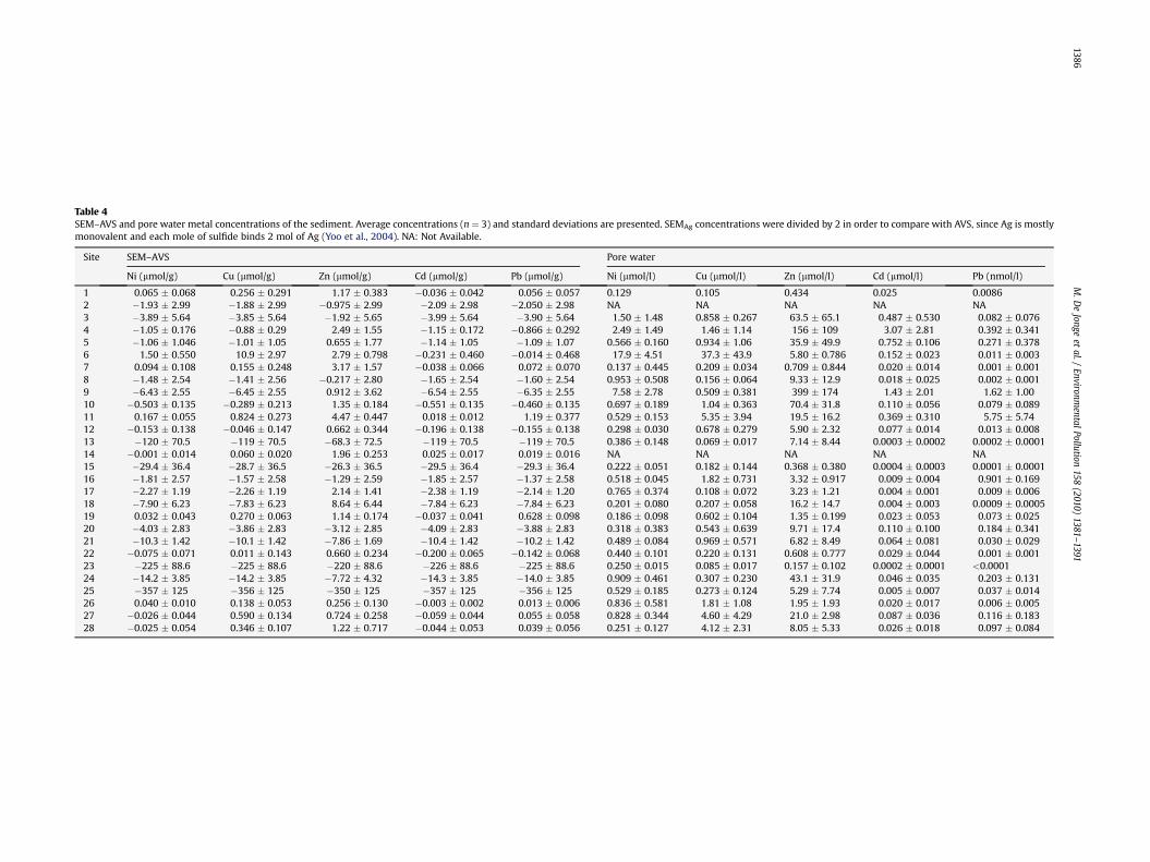
Table 4SEM–AVS and pore water metal concentrations of the sediment. Average concentrations (n ¼ 3) and standard deviations are presented. SEMAg concentrations were divided by 2 in order to compare with AVS, since Ag is mostlymonovalent and each mole of sulfide binds 2 mol of Ag (Yoo et al., 2004). NA: Not Available.

Site SEM–AVS Pore water

Ni (mmol/g) Cu (mmol/g) Zn (mmol/g) Cd (mmol/g) Pb (mmol/g) Ni (mmol/l) Cu (mmol/l) Zn (mmol/l) Cd (mmol/l) Pb (nmol/l)

1 0.065 � 0.068 0.256 � 0.291 1.17 � 0.383 �0.036 � 0.042 0.056 � 0.057 0.129 0.105 0.434 0.025 0.00862 �1.93 � 2.99 �1.88 � 2.99 �0.975 � 2.99 �2.09 � 2.98 �2.050 � 2.98 NA NA NA NA NA3 �3.89 � 5.64 �3.85 � 5.64 �1.92 � 5.65 �3.99 � 5.64 �3.90 � 5.64 1.50 � 1.48 0.858 � 0.267 63.5 � 65.1 0.487 � 0.530 0.082 � 0.0764 �1.05 � 0.176 �0.88 � 0.29 2.49 � 1.55 �1.15 � 0.172 �0.866 � 0.292 2.49 � 1.49 1.46 � 1.14 156 � 109 3.07 � 2.81 0.392 � 0.3415 �1.06 � 1.046 �1.01 � 1.05 0.655 � 1.77 �1.14 � 1.05 �1.09 � 1.07 0.566 � 0.160 0.934 � 1.06 35.9 � 49.9 0.752 � 0.106 0.271 � 0.3786 1.50 � 0.550 10.9 � 2.97 2.79 � 0.798 �0.231 � 0.460 �0.014 � 0.468 17.9 � 4.51 37.3 � 43.9 5.80 � 0.786 0.152 � 0.023 0.011 � 0.0037 0.094 � 0.108 0.155 � 0.248 3.17 � 1.57 �0.038 � 0.066 0.072 � 0.070 0.137 � 0.445 0.209 � 0.034 0.709 � 0.844 0.020 � 0.014 0.001 � 0.0018 �1.48 � 2.54 �1.41 � 2.56 �0.217 � 2.80 �1.65 � 2.54 �1.60 � 2.54 0.953 � 0.508 0.156 � 0.064 9.33 � 12.9 0.018 � 0.025 0.002 � 0.0019 �6.43 � 2.55 �6.45 � 2.55 0.912 � 3.62 �6.54 � 2.55 �6.35 � 2.55 7.58 � 2.78 0.509 � 0.381 399 � 174 1.43 � 2.01 1.62 � 1.0010 �0.503 � 0.135 �0.289 � 0.213 1.35 � 0.184 �0.551 � 0.135 �0.460 � 0.135 0.697 � 0.189 1.04 � 0.363 70.4 � 31.8 0.110 � 0.056 0.079 � 0.08911 0.167 � 0.055 0.824 � 0.273 4.47 � 0.447 0.018 � 0.012 1.19 � 0.377 0.529 � 0.153 5.35 � 3.94 19.5 � 16.2 0.369 � 0.310 5.75 � 5.7412 �0.153 � 0.138 �0.046 � 0.147 0.662 � 0.344 �0.196 � 0.138 �0.155 � 0.138 0.298 � 0.030 0.678 � 0.279 5.90 � 2.32 0.077 � 0.014 0.013 � 0.00813 �120 � 70.5 �119 � 70.5 �68.3 � 72.5 �119 � 70.5 �119 � 70.5 0.386 � 0.148 0.069 � 0.017 7.14 � 8.44 0.0003 � 0.0002 0.0002 � 0.000114 �0.001 � 0.014 0.060 � 0.020 1.96 � 0.253 0.025 � 0.017 0.019 � 0.016 NA NA NA NA NA15 �29.4 � 36.4 �28.7 � 36.5 �26.3 � 36.5 �29.5 � 36.4 �29.3 � 36.4 0.222 � 0.051 0.182 � 0.144 0.368 � 0.380 0.0004 � 0.0003 0.0001 � 0.000116 �1.81 � 2.57 �1.57 � 2.58 �1.29 � 2.59 �1.85 � 2.57 �1.37 � 2.58 0.518 � 0.045 1.82 � 0.731 3.32 � 0.917 0.009 � 0.004 0.901 � 0.16917 �2.27 � 1.19 �2.26 � 1.19 2.14 � 1.41 �2.38 � 1.19 �2.14 � 1.20 0.765 � 0.374 0.108 � 0.072 3.23 � 1.21 0.004 � 0.001 0.009 � 0.00618 �7.90 � 6.23 �7.83 � 6.23 8.64 � 6.44 �7.84 � 6.23 �7.84 � 6.23 0.201 � 0.080 0.207 � 0.058 16.2 � 14.7 0.004 � 0.003 0.0009 � 0.000519 0.032 � 0.043 0.270 � 0.063 1.14 � 0.174 �0.037 � 0.041 0.628 � 0.098 0.186 � 0.098 0.602 � 0.104 1.35 � 0.199 0.023 � 0.053 0.073 � 0.02520 �4.03 � 2.83 �3.86 � 2.83 �3.12 � 2.85 �4.09 � 2.83 �3.88 � 2.83 0.318 � 0.383 0.543 � 0.639 9.71 � 17.4 0.110 � 0.100 0.184 � 0.34121 �10.3 � 1.42 �10.1 � 1.42 �7.86 � 1.69 �10.4 � 1.42 �10.2 � 1.42 0.489 � 0.084 0.969 � 0.571 6.82 � 8.49 0.064 � 0.081 0.030 � 0.02922 �0.075 � 0.071 0.011 � 0.143 0.660 � 0.234 �0.200 � 0.065 �0.142 � 0.068 0.440 � 0.101 0.220 � 0.131 0.608 � 0.777 0.029 � 0.044 0.001 � 0.00123 �225 � 88.6 �225 � 88.6 �220 � 88.6 �226 � 88.6 �225 � 88.6 0.250 � 0.015 0.085 � 0.017 0.157 � 0.102 0.0002 � 0.0001 <0.000124 �14.2 � 3.85 �14.2 � 3.85 �7.72 � 4.32 �14.3 � 3.85 �14.0 � 3.85 0.909 � 0.461 0.307 � 0.230 43.1 � 31.9 0.046 � 0.035 0.203 � 0.13125 �357 � 125 �356 � 125 �350 � 125 �357 � 125 �356 � 125 0.529 � 0.185 0.273 � 0.124 5.29 � 7.74 0.005 � 0.007 0.037 � 0.01426 0.040 � 0.010 0.138 � 0.053 0.256 � 0.130 �0.003 � 0.002 0.013 � 0.006 0.836 � 0.581 1.81 � 1.08 1.95 � 1.93 0.020 � 0.017 0.006 � 0.00527 �0.026 � 0.044 0.590 � 0.134 0.724 � 0.258 �0.059 � 0.044 0.055 � 0.058 0.828 � 0.344 4.60 � 4.29 21.0 � 2.98 0.087 � 0.036 0.116 � 0.18328 �0.025 � 0.054 0.346 � 0.107 1.22 � 0.717 �0.044 � 0.053 0.039 � 0.056 0.251 � 0.127 4.12 � 2.31 8.05 � 5.33 0.026 � 0.018 0.097 � 0.084

M.D

eJonge

etal./

Environmental

Pollution158

(2010)1381–1391

1386

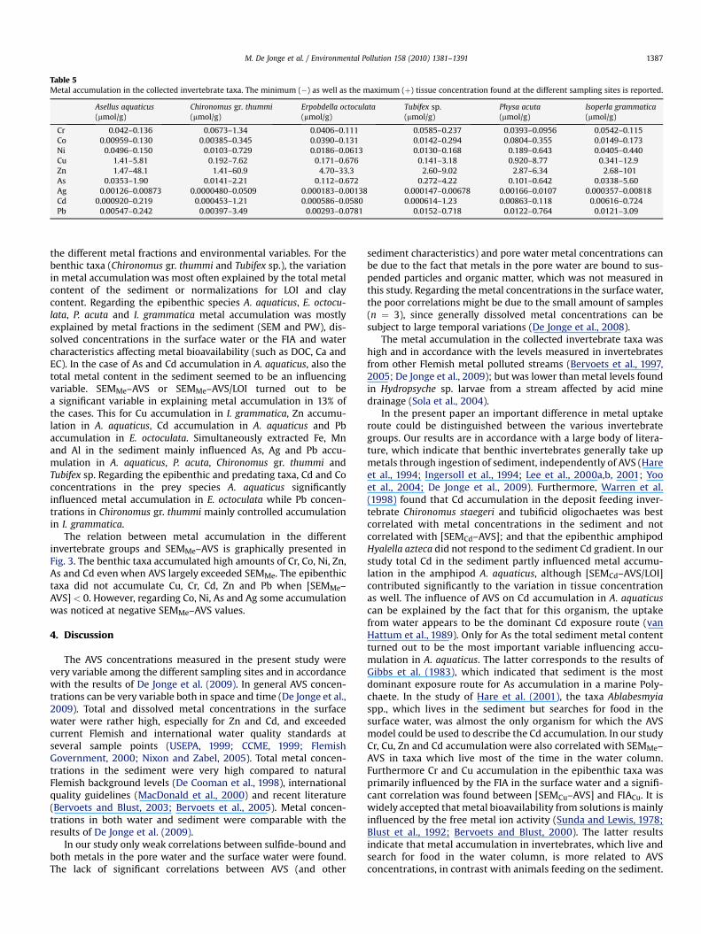
Table 5Metal accumulation in the collected invertebrate taxa. The minimum (�) as well as the maximum (þ) tissue concentration found at the different sampling sites is reported.

Asellus aquaticus(mmol/g)

Chironomus gr. thummi(mmol/g)

Erpobdella octoculata(mmol/g)

Tubifex sp.(mmol/g)

Physa acuta(mmol/g)

Isoperla grammatica(mmol/g)

Cr 0.042–0.136 0.0673–1.34 0.0406–0.111 0.0585–0.237 0.0393–0.0956 0.0542–0.115Co 0.00959–0.130 0.00385–0.345 0.0390–0.131 0.0142–0.294 0.0804–0.355 0.0149–0.173Ni 0.0496–0.150 0.0103–0.729 0.0186–0.0613 0.0130–0.168 0.189–0.643 0.0405–0.440Cu 1.41–5.81 0.192–7.62 0.171–0.676 0.141–3.18 0.920–8.77 0.341–12.9Zn 1.47–48.1 1.41–60.9 4.70–33.3 2.60–9.02 2.87–6.34 2.68–101As 0.0353–1.90 0.0141–2.21 0.112–0.672 0.272–4.22 0.101–0.642 0.0338–5.60Ag 0.00126–0.00873 0.0000480–0.0509 0.000183–0.00138 0.000147–0.00678 0.00166–0.0107 0.000357–0.00818Cd 0.000920–0.219 0.000453–1.21 0.000586–0.0580 0.000614–1.23 0.00863–0.118 0.00616–0.724Pb 0.00547–0.242 0.00397–3.49 0.00293–0.0781 0.0152–0.718 0.0122–0.764 0.0121–3.09

M. De Jonge et al. / Environmental Pollution 158 (2010) 1381–1391 1387

the different metal fractions and environmental variables. For thebenthic taxa (Chironomus gr. thummi and Tubifex sp.), the variationin metal accumulation was most often explained by the total metalcontent of the sediment or normalizations for LOI and claycontent. Regarding the epibenthic species A. aquaticus, E. octocu-lata, P. acuta and I. grammatica metal accumulation was mostlyexplained by metal fractions in the sediment (SEM and PW), dis-solved concentrations in the surface water or the FIA and watercharacteristics affecting metal bioavailability (such as DOC, Ca andEC). In the case of As and Cd accumulation in A. aquaticus, also thetotal metal content in the sediment seemed to be an influencingvariable. SEMMe–AVS or SEMMe–AVS/LOI turned out to bea significant variable in explaining metal accumulation in 13% ofthe cases. This for Cu accumulation in I. grammatica, Zn accumu-lation in A. aquaticus, Cd accumulation in A. aquaticus and Pbaccumulation in E. octoculata. Simultaneously extracted Fe, Mnand Al in the sediment mainly influenced As, Ag and Pb accu-mulation in A. aquaticus, P. acuta, Chironomus gr. thummi andTubifex sp. Regarding the epibenthic and predating taxa, Cd and Coconcentrations in the prey species A. aquaticus significantlyinfluenced metal accumulation in E. octoculata while Pb concen-trations in Chironomus gr. thummi mainly controlled accumulationin I. grammatica.

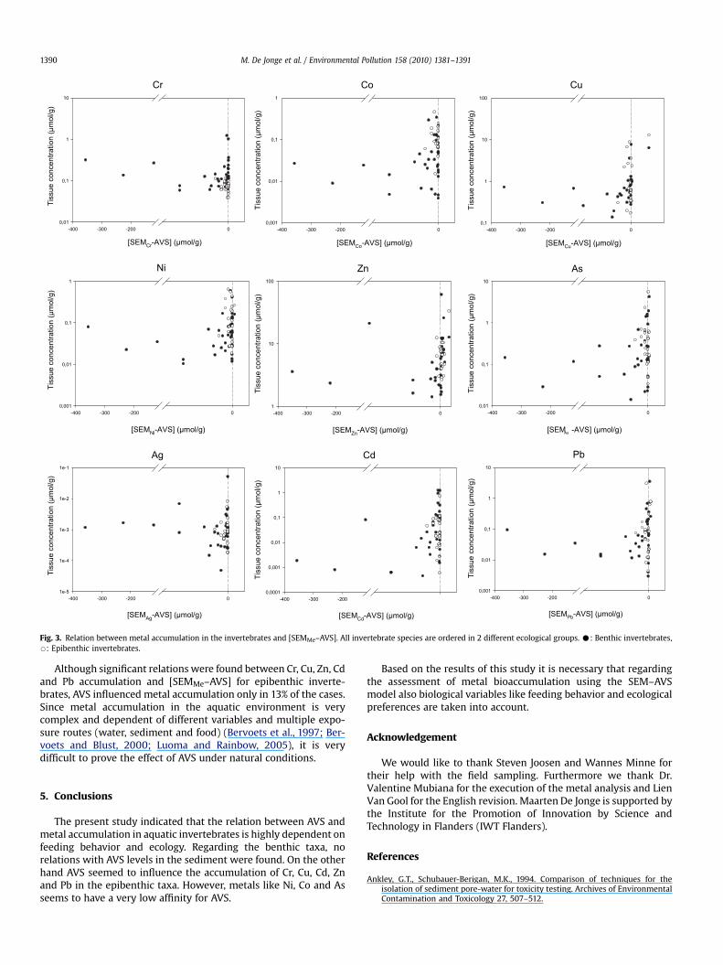
The relation between metal accumulation in the differentinvertebrate groups and SEMMe–AVS is graphically presented inFig. 3. The benthic taxa accumulated high amounts of Cr, Co, Ni, Zn,As and Cd even when AVS largely exceeded SEMMe. The epibenthictaxa did not accumulate Cu, Cr, Cd, Zn and Pb when [SEMMe–AVS] < 0. However, regarding Co, Ni, As and Ag some accumulationwas noticed at negative SEMMe–AVS values.

4. Discussion

The AVS concentrations measured in the present study werevery variable among the different sampling sites and in accordancewith the results of De Jonge et al. (2009). In general AVS concen-trations can be very variable both in space and time (De Jonge et al.,2009). Total and dissolved metal concentrations in the surfacewater were rather high, especially for Zn and Cd, and exceededcurrent Flemish and international water quality standards atseveral sample points (USEPA, 1999; CCME, 1999; FlemishGovernment, 2000; Nixon and Zabel, 2005). Total metal concen-trations in the sediment were very high compared to naturalFlemish background levels (De Cooman et al., 1998), internationalquality guidelines (MacDonald et al., 2000) and recent literature(Bervoets and Blust, 2003; Bervoets et al., 2005). Metal concen-trations in both water and sediment were comparable with theresults of De Jonge et al. (2009).

In our study only weak correlations between sulfide-bound andboth metals in the pore water and the surface water were found.The lack of significant correlations between AVS (and other

sediment characteristics) and pore water metal concentrations canbe due to the fact that metals in the pore water are bound to sus-pended particles and organic matter, which was not measured inthis study. Regarding the metal concentrations in the surface water,the poor correlations might be due to the small amount of samples(n ¼ 3), since generally dissolved metal concentrations can besubject to large temporal variations (De Jonge et al., 2008).

The metal accumulation in the collected invertebrate taxa washigh and in accordance with the levels measured in invertebratesfrom other Flemish metal polluted streams (Bervoets et al., 1997,2005; De Jonge et al., 2009); but was lower than metal levels foundin Hydropsyche sp. larvae from a stream affected by acid minedrainage (Sola et al., 2004).

In the present paper an important difference in metal uptakeroute could be distinguished between the various invertebrategroups. Our results are in accordance with a large body of litera-ture, which indicate that benthic invertebrates generally take upmetals through ingestion of sediment, independently of AVS (Hareet al., 1994; Ingersoll et al., 1994; Lee et al., 2000a,b, 2001; Yooet al., 2004; De Jonge et al., 2009). Furthermore, Warren et al.(1998) found that Cd accumulation in the deposit feeding inver-tebrate Chironomus staegeri and tubificid oligochaetes was bestcorrelated with metal concentrations in the sediment and notcorrelated with [SEMCd–AVS]; and that the epibenthic amphipodHyalella azteca did not respond to the sediment Cd gradient. In ourstudy total Cd in the sediment partly influenced metal accumu-lation in the amphipod A. aquaticus, although [SEMCd–AVS/LOI]contributed significantly to the variation in tissue concentrationas well. The influence of AVS on Cd accumulation in A. aquaticuscan be explained by the fact that for this organism, the uptakefrom water appears to be the dominant Cd exposure route (vanHattum et al., 1989). Only for As the total sediment metal contentturned out to be the most important variable influencing accu-mulation in A. aquaticus. The latter corresponds to the results ofGibbs et al. (1983), which indicated that sediment is the mostdominant exposure route for As accumulation in a marine Poly-chaete. In the study of Hare et al. (2001), the taxa Ablabesmyiaspp., which lives in the sediment but searches for food in thesurface water, was almost the only organism for which the AVSmodel could be used to describe the Cd accumulation. In our studyCr, Cu, Zn and Cd accumulation were also correlated with SEMMe–AVS in taxa which live most of the time in the water column.Furthermore Cr and Cu accumulation in the epibenthic taxa wasprimarily influenced by the FIA in the surface water and a signifi-cant correlation was found between [SEMCu–AVS] and FIACu. It iswidely accepted that metal bioavailability from solutions is mainlyinfluenced by the free metal ion activity (Sunda and Lewis, 1978;Blust et al., 1992; Bervoets and Blust, 2000). The latter resultsindicate that metal accumulation in invertebrates, which live andsearch for food in the water column, is more related to AVSconcentrations, in contrast with animals feeding on the sediment.

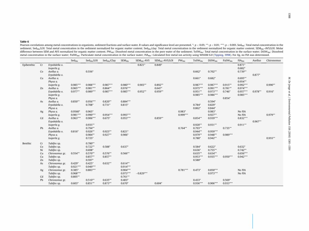
Table 6Pearson correlations among metal concentrations in organisms, sediment fractions and surface water. R-values and significance level are presented. *: p < 0.05; **: p < 0.01; ***: p < 0.001. SedMe: Total metal concentration in thesediment; SedMe/LOI: Total metal concentration in the sediment normalized for organic matter content; SedMe/clay: Total metal concentration in the sediment normalized for organic matter content; SEMMe–AVS/LOI: Molardifference between SEM and AVS normalized for organic matter content; PWME: Dissolved metal concentration in the pore water of the sediment; ToSWMe: Total metal concentration in the surface water; DiSWMe: Dissolvedmetal concentration in the surface water; PaSWMe: Particulate metal concentration in the surface water; FIAMe: Calculated free metal ion activity using WHAM 6.0 (Tipping, 1998). For Ag, no FIA was determined.

SedMe SedMe/LOI SedMe/Clay SEMMe SEMMe-AVS SEMMe-AVS/LOI PWMe ToSWMe DiSWMe PaSWMe FIAMe Asellus Chironomus

Epibenthic Cr Erpobdella o. 0.821* 0.849* 0.871*Isoperla g. 0.682*

Co Asellus a. 0.556* 0.662* 0.702** 0.739**Erpobdella o. 0.877*

Cu Asellus a. 0.661* 0.682* 0.695**Physa a. 0.954**Isoperla g. 0.985*** 0.988*** 0.987*** 0.980*** 0.903** 0.892** 0.987*** 0.987*** 0.915** 0.992*** 0.990**

Zn Asellus a. 0.965*** 0.981*** 0.864** 0.976*** 0.647* 0.975*** 0.991*** 0.781** 0.974***Erpobdella o. 0.977** 0.989*** 0.987*** 0.985*** 0.952** 0.959** 0.951** 0.973*** 0.746* 0.957*** 0.978** 0.916*Isoperla g. 0.985*** 0.986*** 0.985***Physa a. 0.854*

As Asellus a. 0.850** 0.956*** 0.820** 0.884*** 0.594*Erpobdella o. 0.708* 0.731* 0.815* 0.784* 0.829*Physa a. 0.862* 0.844*

Ag Physa a. 0.9560* 0.965* 0.983* 0.983* No FIAIsoperla g. 0.981*** 0.990*** 0.954*** 0.993*** 0.999*** 0.927** No FIA 0.979**

Cd Asellus a. 0.963*** 0.906*** 0.675* 0.953*** 0.859** 0.854** 0.939*** 0.832***Erpobdella o. 0.967**Isoperla g. 0.935** 0.920** 0.931** 0.911**

Pb Asellus a. 0.794** 0.764** 0.793** 0.735**Erpobdella o. 0.816* 0.926** 0.923** 0.821* 0.944** 0.959***Physa a. 0.984** 0.927** 0.906* 0.979** 0.948** 0.989***Isoperla g. 0.725* 0.780* 0.942** 0.955**

Benthic Cr Tubifex sp. 0.780**Co Tubifex sp. 0.722** 0.588* 0.637* 0.584* 0.622* 0.632*Ni Tubifex sp. 0.698* 0.636* 0.755** 0.742**Cu Chironomus gr. 0.554** 0.570** 0.576** 0.566** 0.635** 0.634** 0.656***Cu Tubifex sp. 0.857** 0.857** 0.953*** 0.935*** 0.950*** 0.942***Zn Tubifex sp. 0.597* 0.580*As Chironomus gr. 0.429* 0.425* 0.632** 0.614**

Tubifex sp. 0.921*** 0.949*** 0.914***Ag Chironomus gr. 0.385* 0.883*** 0.904*** 0.781*** 0.473* 0.850*** No FIA

Tubifex sp. 0.968*** 0.973*** �0.829*** 0.973*** No FIACd Tubifex sp. 0.805** 0.761**Pb Chironomus gr. 0.510** 0.635** 0.403* 0.433* 0.569*

Tubifex sp. 0.603* 0.851** 0.873** 0.670* 0.604* 0.936*** 0.906*** 0.933***

M.D

eJonge

etal./

Environmental

Pollution158

(2010)1381–1391

1388

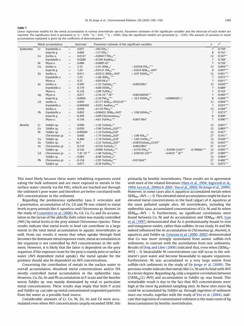
Table 7Linear regression models for the metal accumulation in various invertebrate species. Parameter estimates of the significant variables and the intercept of each model arereported. The significance level is presented as *p < 0.05; **p < 0.01; ***p < 0.001. Only the significant models are presented (p < 0.05). The amount of variation in metalaccumulation explained is given by the coefficient of determination r2.

Metal accumulation Intercept Parameter estimate of the significant variables n r2

Epibenthic Cr Erpobdella o. ¼ 0.057 þ592 FIACr* 7 0.758*Isoperla g. ¼ 0.069 þ117 FIACr* 8 0.741*

Co Asellus a. ¼ 0.0127 þ0.00417 FIACo** 12 0.547**Erpobdella o. ¼ 0.0280 þ0.549 AsellusCo* 7 0.768*

Ni Physa a. ¼ 0.088 þ0.0005 EC* 7 0.728*Cu Asellus a. ¼ 2.33 þ2.91 SEMCu* þ 0.0558 FIACu*** 12 0.894***

Isoperla g. ¼ 1.29 þ0.0131 FIACu*** þ 0.024 SEMCu–AVS* 8 0.997***Zn Asellus a. ¼ 0.611 þ0.0212 SEMZn-AVS* þ 4.97 DiSWZn*** 12 0.991***

Erpobdella o. ¼ 5.25 þ1.66 SEMZn *** 7 0.972***Physa a. ¼ 9.21 �0.0519Ca** 7 0.851**

As Asellus a. ¼ 0.285 þ1.22 TotSedAs*** �0.00220Fe* 12 0.820***Erpobdella o. ¼ 0.179 þ6.80 DiSWAs* 7 0.680*Physa a. ¼ 0.126 þ3.08 ToSWAs* 7 0.743*

Ag Physa a. ¼ 0.017 þ2.54 10�5 Al** �0.00166DOC** 7 0.999***Isoperla g. ¼ �0.0005 þ5.20 PWAg*** þ 10.5 DiSWAg** �0.0000569�2* 8 0.999***

Cd Asellus a. ¼ 0.003 þ0.177 SEMCd–AVS/LOI*** 12 0.984***Erpobdella o. ¼ �0.000439 þ0.651 AsellusCd*** 7 0.935***Asellus a. ¼ 0.058 þ0.119 PWPb** 12 0.584**

Pb Erpobdella o. ¼ 0.002 þ0.00432 SEMPb-AVS* þ 5.98 DiSWPb** 7 0.973**Isoperla g. ¼ �0.369 þ6.89 ChironomusPb* 8 0.906*Physa a. ¼ 0.156 þ4.61 PaSWPb*** �0.00176Fe* 7 0.996***

Benthic Cr Tubifex sp. ¼ 0.006 þ1.42 TotSedCr** 12 0.661**Co Tubifex sp. ¼ �0.050 þ5.96 TotSedCo/LOI*** 12 0.869***Ni Tubifex sp. ¼ �0.00260 þ1.16 TotSedNi/LOI* 12 0.437*

Chironomus gr. ¼ 0.666 þ1.74 TotSedCu/LOI* þ 3.89 FIACu** 27 0.541**Cu Tubifex sp. ¼ 0.406 þ1.74 TotSedCu/LOI* þ 3.89 ToSWCu** 12 0.938***Zn Tubifex sp. ¼ 10.7 þ2.23 TotSedZn/LOI** �0.683TotSedZn/CLAY* 12 0.943***As Chironomus gr. ¼ 0.210 þ0.534 TotSedAs** �0.00228Fe* 27 0.316**

Tubifex sp. ¼ 0.142 þ0.969 TotSedAs*** þ 0.576 PWAs** þ 0.0399 CLAY** �0.790Mn*** 12 0.995***Cd Chironomus gr. ¼ 7.41 10�4 þ1.48 TotSedAg*** þ 0.00105 LOI*** �4.4410�3 Al** 27 0.980***

Tubifex sp. ¼ �0.083 þ8.88 TotSedCd** 12 0.984**Pb Chironomus gr. ¼ �0.154 þ2.95 TotSedPb*** �0.0136Al** 27 0.486***

Tubifex sp. ¼ 0.077 þ6.30 PaSWPb*** 12 0.875***

M. De Jonge et al. / Environmental Pollution 158 (2010) 1381–1391 1389

This most likely because these water inhabiting organisms avoideating the bulk sediment and are more exposed to metals in thesurface water (mostly via the FIA), which are leached out throughthe sediment’s pore water and therefore are better correlated withAVS concentrations in the sediment.

Regarding the predatorous epibenthic taxa E. octoculata andI. grammatica, accumulation of Co, Cd and Pb was related to metallevels in prey animals like A. aquaticus and Chironomus gr. thummi. Inthe study of Croisetiere et al. (2006) As, Cd, Co, Cu and Zn accumu-lation in the larvae of the alderfly Sialis velata was mainly controlled(94%) by metal levels in the prey animal Chironomus riparius. Theseresults indicate that metal levels in food can contribute in a largeextent to the total metal accumulation in aquatic invertebrates aswell. From our results it seems that when uptake through foodbecomes the dominant metal exposure route, metal accumulation inthe organism is not controlled by AVS concentrations in the sedi-ment. However, it is likely that the latter is dependent on the preyorganism. If the exposure route for the prey is mainly pore or surfacewater (AVS dependent metal uptake), the metal uptake for thepredator should also be dependent on AVS concentrations.

Concerning the contribution of metals in the surface water tooverall accumulation, dissolved metal concentrations and/or FIAmostly controlled metal accumulation in the epibenthic taxa.However, Cu, Zn, As and Pb accumulation in P. acuta and the benthicworm Tubifex sp. was mainly dominated by total or particulatemetal concentrations. These results may imply that both P. acutaand Tubifex sp. can take up metal contaminated suspended particlesfrom the water as a possible food source.

Considerable amounts of Cr, Co, Ni, Zn, As and Cd were accu-mulated even when AVS concentrations largely exceeded SEM; this

primarily by benthic invertebrates. These results are in agreementwith most of the related literature (Hare et al., 1994; Ingersoll et al.,1994; Lee et al., 2000a,b, 2001; Yoo et al., 2004; De Jonge et al., 2009).However, in some cases also A. aquaticus accumulated metals whenSEMMe–AVS<<0. This elevated metal accumulation might be due toelevated metal concentrations in the food (algae) of A. aquaticus atthe most polluted sample sites. All invertebrates, including theepibenthic taxa, accumulated concentrations of Co, Ni and As whenSEMMe–AVS < 0. Furthermore, no significant correlations werefound between Co, Ni and As accumulation and SEMMe–AVS. Guoet al. (1997) demonstrated that As is predominantly bound to ironand manganese oxides, rather than sulfides. In our study, Fe and Mnindeed influenced the As accumulation in Chironomus gr. thummi, A.aquaticus and Tubifex sp. Griscom et al. (2000, 2002) demonstratedthat Co was more strongly assimilated from anoxic sulfide-richsediments, in contrast with the assimilation from oxic sediments.Results of Doig and Liber (2006) indicated that, even when [SEMNi–AVS] < 0, bioavailable Ni concentrations can still occur in the sed-iment’s pore water and become bioavailabe to aquatic organisms.Furthermore, Ni was accumulated to a very large extent fromsulfide-rich sediments in the study of De Jonge et al. (2009). Theprevious results indicate that metals like Co, Ni and As bind with AVSto a lesser degree. Regarding Ag, only a negative correlation between[(SEMAg/2)–AVS] and accumulation in Tubifex sp. was found. Thisremarkable result is due to the fact that AVS concentrations werehigh at the most Ag polluted sampling sites. At these sites more Agcould be accumulated by Tubifex sp. through ingestion of sedimentsince our results, together with the study of Yoo et al. (2004), indi-cate that ingestion of contaminated sediment is the main route of Agbioaccumulation by benthic invertebrates.

Cr

[SEMCr-AVS] (µmol/g)

0002-003-004-

Tiss

ue c

once

ntra

tion

(µm

ol/g

)

0,01

0,1

1

10

Ni

[SEMNi-AVS] (µmol/g)

0002-003-004-

Tiss

ue c

once

ntra

tion

(µm

ol/g

)

0,001

0,01

0,1

1

Ag

[SEMAg-AVS] (µmol/g)

0002-003-004-

Tiss

ue c

once

ntra

tion

(µm

ol/g

)

1e-5

1e-4

1e-3

1e-2

1e-1

Co

[SEMCo-AVS] (µmol/g)

0002-003-004-

Tiss

ue c

once

ntra

tion

(µm

ol/g

)

0,001

0,01

0,1

1

Zn

[SEMZn-AVS] (µmol/g)

0002-003-004-

Tiss

ue c

once

ntra

tion

(µm

ol/g

)

1

10

100

Cd

[SEMCd-AVS] (µmol/g)

002-003-004-

Tiss

ue c

once

ntra

tion

(µm

ol/g

)

0,0001

0,001

0,01

0,1

1

10

Cu

[SEMCu-AVS] (µmol/g)

0002-003-004-

Tiss

ue c

once

ntra

tion

(µm

ol/g

)

0,1

1

10

100

As

[SEMAs -AVS] (µmol/g)

0002-003-004-

Tiss

ue c

once

ntra

tion

(µm

ol/g

)

0,01

0,1

1

10

Pb

[SEMPb-AVS] (µmol/g)

0002-003-004-

Tiss

ue c

once

ntra

tion

(µm

ol/g

)

0,001

0,01

0,1

1

10

Fig. 3. Relation between metal accumulation in the invertebrates and [SEMMe–AVS]. All invertebrate species are ordered in 2 different ecological groups. C: Benthic invertebrates,B: Epibenthic invertebrates.

M. De Jonge et al. / Environmental Pollution 158 (2010) 1381–13911390

Although significant relations were found between Cr, Cu, Zn, Cdand Pb accumulation and [SEMMe–AVS] for epibenthic inverte-brates, AVS influenced metal accumulation only in 13% of the cases.Since metal accumulation in the aquatic environment is verycomplex and dependent of different variables and multiple expo-sure routes (water, sediment and food) (Bervoets et al., 1997; Ber-voets and Blust, 2000; Luoma and Rainbow, 2005), it is verydifficult to prove the effect of AVS under natural conditions.

5. Conclusions

The present study indicated that the relation between AVS andmetal accumulation in aquatic invertebrates is highly dependent onfeeding behavior and ecology. Regarding the benthic taxa, norelations with AVS levels in the sediment were found. On the otherhand AVS seemed to influence the accumulation of Cr, Cu, Cd, Znand Pb in the epibenthic taxa. However, metals like Ni, Co and Asseems to have a very low affinity for AVS.

Based on the results of this study it is necessary that regardingthe assessment of metal bioaccumulation using the SEM–AVSmodel also biological variables like feeding behavior and ecologicalpreferences are taken into account.

Acknowledgement

We would like to thank Steven Joosen and Wannes Minne fortheir help with the field sampling. Furthermore we thank Dr.Valentine Mubiana for the execution of the metal analysis and LienVan Gool for the English revision. Maarten De Jonge is supported bythe Institute for the Promotion of Innovation by Science andTechnology in Flanders (IWT Flanders).

References

Ankley, G.T., Schubauer-Berigan, M.K., 1994. Comparison of techniques for theisolation of sediment pore-water for toxicity testing. Archives of EnvironmentalContamination and Toxicology 27, 507–512.

M. De Jonge et al. / Environmental Pollution 158 (2010) 1381–1391 1391

Berry, W.J., Boothman, W.S., Serbst, J.R., Edwards, P.A., 2004. Predicting the toxicityof chromium in sediments. Environmental Toxicology and Chemistry 23,2981–2992.

Bervoets, L., Blust, R., 2000. Effects of pH on cadmium and zinc uptake by the midgelarvae Chironomus riparius. Aquatic Toxicology 49, 145–157.

Bervoets, L., Blust, R., 2003. Metal concentrations in water, sediment and gudgeon(Gobio gobio) from a pollution gradient: relationship with fish condition factor.Environmental Pollution 126, 9–19.

Bervoets, L., Blust, R., de Wit, M., Verheyen, R., 1997. Relationships between riversediment characteristics and trace metal concentrations in Tubificid worms andChironomid larvae. Environmental Pollution 95, 345–356.

Bervoets, L., Voets, J., Covaci, A., Chu, S.G., Qadah, D., Smolders, R., Schepens, P.,Blust, R., 2005. Use of transplanted zebra mussels (Dreissena polymorpha) toassess the bioavailability of microcontaminants in Flemish surface waters.Environmental Science and Technology 39, 1492–1505.

Blust, R., Van der Linden, A., Verheyen, E., Decleir, W., 1988. Evaluation of micro-wave heating digestion and graphite furnace atomic absorption spectrometrywith continuum source background correction for the determination of Fe,Cu and Cd in brine shrimp. Journal of Analytical Atomic Spectrometry 3,387–393.

Blust, R., Kockelbergh, E., Baillieul, M., 1992. Effect of salinity on the uptake ofcadmium by the brine shrimp Artemia franciscana. Marine Ecology ProgressSeries 84, 245–254.

Canadian Council of Ministers of the Environment (CCME), 1999. Canadian Envi-ronmental Quality Guidelines, Winnipeg, MB, Canada.

Croisetiere, L., Hare, L., Tessier, A., 2006. A field experiment to determine therelative importance of prey and water as sources of As, Cd, Co, Cu, Pb and Zn forthe aquatic invertebrate Sialis velata. Environmental Science and Technology 40,873–879.

Davis, J.A., Leckie, J.O., 1978. Effect of adsorbed complexing ligands on trace metaluptake by hydrons oxides. Environmental Science and Technology 12, 1309–1315.

De Cooman, W., Florus, M., Devroede, M.P., 1998. Characterization of Sediments ofFlemish Watercourses. Ministry of the Flemish Government, Brussels, Belgium.

De Jonge, M., Van de Vijver, B., Blust, R., Bervoets, L., 2008. Responses of aquaticorganisms to metal pollution in a lowland river in Flanders: a comparison ofdiatoms and macroinvertebrates. Science of the Total Environment 407,615–629.

De Jonge, M., Dreesen, F., De Paepe, J., Blust, R., Bervoets, L., 2009. Do Acid VolatileSulfides (AVS) influence the accumulation of sediment-bound metals to benthicinvertebrates under natural field conditions? Environmental Science andTechnology 43, 4510–4516.

de Lange, H.J., van Griethuysen, C., Koelmans, A.A., 2008. Sampling method, storageand pretreatment of sediment affect AVS concentrations with consequences forbioassay responses. Environmental Pollution 151, 243–251.

Di Toro, D.M., Mahony, J.D., Hansen, D.J., Scott, K.J., Carlson, A., Ankley, G.T., 1992.Acid Volatile Sulphide predicts the acute toxicity of cadmium and nickel insediments. Environmental Science and Technology 26, 96–101.

Di Toro, D.M., Mahony, J.D., Hansen, D.J., Scott, K.J., Hicks, M.B., Mays, S.M.,Redmond, M.S., 1990. Toxicity of cadmium in sediments: the role of acid volatilesulfides. Environmental Toxicology and Chemistry 9, 1487–1502.

Doig, L.E., Liber, K., 2006. Influence of dissolved organic matter on nickel bioavail-ability and toxicity to Hyalella azteca in water-only exposures. Aquatic Toxi-cology 78, 203–216.

Elliott, J.M., 2004. Prey switching in four species of carnivorous stoneflies. Fresh-water Biology 49, 709–720.

Flemish Government, 2000. Besluit van de Vlaamse Regering van 1 juni 1995houdende vaststelling van het Vlaamse reglement betreffende de milieu-vergunning (Vlarem), zoals gewijzigd bij besluit van 17 juli 2000. BelgischStaatsblad. 5 augustus 2000 (in Dutch).

Gibbs, P.E., Langston, W.J., Burt, G.R., Pascoe, P.L., 1983. Tharyx marioni (Polychaeta) –a remarkable accumulator of arsenic. Journal of the Marine Biological Associ-ation of the United Kingdom 63, 313–325.

Goodyear, K.L., McNeill, S., 1999. Bioaccumulation of heavy metals by aquaticmacro-invertebrates of different feeding guilds: a review. Science of the TotalEnvironment 229, 1–19.

Griscom, S.B., Fisher, N.S., Luoma, S.N., 2000. Geochemical influences on assimila-tion of sediment-bound metals in clams and mussels. Environmental Scienceand Technology 34, 91–99.

Griscom, S.B., Fisher, N.S., Aller, R.C., Lee, B.-G., 2002. Effects of gut chemistry inmarine bivalves on the assimilation of metals from ingested sediment particles.Journal of Marine Research 60, 101–120.

Guo, T., De Laune, R.D., Patrick Jr., W.H., 1997. The influence of sediment redoxchemistry on chemically active forms of arsenic, cadmium, chromium and zincin estuarine sediment. Environment International 23, 305–316.

Hare, L., Campbell, P.G.C., 1992. Temporal variations of trace metals in aquaticinsects. Freshwater Biology 27, 13–27.

Hare, L., Carignan, R., Huerta-Diaz, M., 1994. A field study of metal toxicity andaccumulation by benthic invertebrates – implications for the acid-volatilesulphide (AVS) model. Limnology and Oceanography 39, 1653–1668.

Hare, L., Tessier, A., Warren, L., 2001. Cadmium accumulation by invertebrates livingat the sediment–water interface. Environmental Toxicology and Chemistry 20,880–889.

Ingersoll, C.G., Brumbaugh, W.G., Dwyer, F.J., Kemble, N.E., 1994. Bioaccumulation ofmetals by Hyalella azteca exposed to contaminated sediments from the upperClark-fork River, Montana. Environmental Toxicology and Chemistry 13,2013–2020.

Kutschera, U., 2003. The feeding strategies of the leech Erpobdella octoculata (L.):a laboratory study. International Review of Hydrobiology 88, 94–101.

Lee, B.-G., Griscom, S.B., Lee, J.-S., Choi, H.-J., Koh, C.-H., Luoma, S.N., Fisher, N.S.,2000a. Influences of dietary uptake and reactive sulfides on metal bioavail-ability from aquatic sediments. Science 287, 282–284.

Lee, B.-G., Lee, J.-S., Luoma, S.N., Choi, H.-J., Koh, C.-H., 2000b. Influence of AcidVolatile Sulfide and metal concentrations on metal bioavailability to marineinvertebrates in contaminated sediments. Environmental Science and Tech-nology 34, 4511–4516.

Lee, J.-S., Lee, B.-G., Yoo, H., Koh, C.-H., Luoma, S.N., 2001. Influence of reactivesulfide (AVS) and supplementary food on Ag, Cd and Zn bioaccumulation in themarine polychaete Neanthes arenaceodentata. Marine Ecology Progress Series216, 129–140.

Leonard, E.N., Cotter, A.M., Ankley, G.T., 1996. Modified diffusion method for anal-ysis of acid volatile sulfides and simultaneously extracted metals in freshwatersediment. Environmental Toxicology and Chemistry 15, 1479–1481.

Luoma, S.N., 1983. Bioavailability of trace metals to aquatic organisms. A review.Science of the Total Environment 28, 1–22.

Luoma, S.N., Rainbow, P.S., 2005. Why is metal bioaccumulation so variable?Biodynamics as a unifying concept. Environmental Science and Technology 39,1921–1931.

MacDonald, D.D., Ingersoll, C.G., Berger, T.A., 2000. Development and evaluation ofconsensus-based sediment quality guidelines for freshwater ecosystems.Archives of Environmental Contamination and Toxicology 39, 20–31.

Nixon, S., Zabel, T., 2005. Proposed environmental quality standards for prioritysubstances – current compliance and potential benefits.

Pennak, R.W., 1989. Fresh-water Invertebrates of the United States, third ed.. Wiley.Queralt, I., Barreiros, M.A., Carvalho, M.L., Costa, M.M., 1999. Application of different

techniques to assess sediment quality and point source pollution in low-levelcontaminated estuarine recent sediments (Lisboa coast, Portugal). Science ofthe Total Environment 241, 39–51.

Sola, C., Burgos, M., Plazuelo, A., Toja, J., Plans, M., Prat, N., 2004. Heavy metalbioaccumulation and macroinvertebrate community changes in a Mediterra-nean stream affected by acid mine drainage and an accidental spill (GuadiamarRiver, SW Spain). Science of the Total Environment 333, 109–126.

Sunda, W.G., Lewis, A.M., 1978. Effect of complexation by natural organic ligands onthe toxicity of copper on unicellular alga, Monochrysis lutheri. Limnology andOceanography 23, 870–876.

Tessier, A., Campbell, P.G.C., Auclair, J.C., Bisson, M., 1984. Relationships between thepartitioning of trace metals in sediments and their accumulation in the tissuesof the freshwater mollusc Elliptio complanata in a mining area. CanadianJournal of Fisheries and Aquatic Sciences 41, 1463–1472.

Tipping, E., 1998. Humic ion-binding model VI: an improved description of theinteractions of protons and metal ions with humic substances. AquaticGeochemistry 4, 3–48.

US Environmental Protection Agency, 1999. National Recommended Water QualityCriteria–Correction. US. EPA, Washington, DC. 822/Z-99–001.

van Hattum, B., De Voogt, P., Van den Bosch, L., van Straalen, N.M., Joosse, E.N.G.,1989. Bioaccumulation of cadmium by the freshwater isopod Asellus aquaticus(L.) from aqueous and dietary sources. Environmental Pollution 62, 129–151.

Warren, L.A., Tessier, A., Hare, L., 1998. Modelling cadmium accumulation by benthicinvertebrates in situ: the relative contributions of sediment and overlying waterreservoirs to organism cadmium concentrations. Limnology and Oceanography43, 1442–1454.

Yoo, H., Lee, J.-S., Lee, B.-G., Lee, I.T., Schlekat, C.E., Koh, C.-H., Luoma, S.N., 2004.Uptake pathway for Ag bioaccumulation in three benthic invertebrates exposedto contaminated sediments. Marine Ecology Progress Series 270, 141–152.