The regression model with one stochastic regressor ...

Regression model with stochastic regressor (RM2) The multiple regression model (I)

The regression model with one stochasticregressor (summary) and multiple regression

(start)

Ragnar Nymoen

University of Oslo

12 February 2013

1 / 22


Summary of Lecture 7 and 8 I

I Assumptions: The n pairs of random variables {Yi ,Xi}i = 1, 2, . . . , n are IID and representative of the populationdistribution function fXY (X ,Y ).

I Argument: With use of factorization of the n identical jointdensities fXY we can establish the conditional expectationfunction, aka the regression function:

E (Yi | Xi = xi ) = β0 + β1Xi ∀ i (1)

with homoskedasticity:

Var(Yi | Xi = xi ) = σ2 ∀ i (2)

2 / 22


Summary of Lecture 7 and 8 II

I Remember that the linearity of E (Yi | Xi = xi ) in mostpractical situations is a result of modelling choices: Variabletransformations and choice of functional form (HGL Ch 4;BN kap 2; Lecture 2 and 7).

I When there is no danger of misunderstanding, we use themore compact notation

E (Yi | Xi ) = β0 + β1Xi ∀ i

Var(Yi | Xi ) = σ2 ∀ i

where is understood that in a given sample of observablerandom variables “| Xi” operates on Xi and turns it into aparameter xi .

3 / 22


Summary of Lecture 7 and 8 III

I The OLS estimators β0 and β1 are unbiased. The proof is bythe use of the theorem of Iterated Expectations (Lect 6 and8), for example

E[E (β1 | X )

]= E [β1] = β1

where we first find the expectation of the function where X isa parameter, namely of E (β1 | X ). This is the same operationas in RM1, giving E (β1 | X ) = β1.

I Inference: Since the distributions of the t−statistics thatwe use for hypothesis testing and confidence intervals areindependent of X , the inference procedures for RM1 are validfor the case with deterministic regressor Xi .

4 / 22


Model specification with disturbance term

Bringing back the disturbance term I

I The disturbance term was a central concept in RM1.

I We can align the two models with regard to the disturbanceterm, and give the model a similar specification as we had forRM1, this will be closer to the typical textbook specification

I As in Ch 10.1.1 in HGL

5 / 22



The disturbances and their properties I

DefinitionWe have {Xi ,Yi} i = 1, 2, . . . , n random variables and theconditional expectation E (Yi | Xi ).Define n new random variablesε i by

ε i := Yi − E (Yi | Xi ) ∀ i (3)

which are the disturbances.Expectation of ε i :

E (ε i | Xi ) = E [(Yi | Xi )]− E (Yi | Xi ) | Xi ] =

= E (Yi | Xi )− E (Yi | Xi ) = 0 (4)

6 / 22



The disturbances and their properties IIConsequence: Exogeneity of Xi : Since the conditionalexpectation of ε i given Xi is constant, we have that (Lecture 6):

Cov(ε i ,Xi ) = 0 (5)

in econometric terminology this is called (strict) exogeneity of Xi

with respect to ε i . This type of exogeneity is generic in ourregression model.Variance of ε i

Var(ε i | Xi ) = Var {(Yi | Xi )− E (Yi | Xi ) | Xi )}

The second term, E (Yi | Xi ) is a parameter for fixed Xi (= xi ),hence

Var(ε i | Xi ) = Var(Yi | Xi ) = σ2 (6)

7 / 22



The disturbances and their properties III

which is the conventional way of stating the homoskedasticityproperty.Covariance:Also from IID:

Cov(ε i , εj | Xi ) = E (ε i εj | Xi ) = Cov(Yi ,Yj | Xi ) = 0 ∀i 6= j(7)

8 / 22



“Classical” model specification and properitesThe model can be specified by the linear relationship:

Yi = β0 + β1Xi + ε i i = 1, 2, . . . , n (8)

and the set of assumptions:

a. Xi (i = 1, 2, . . . , n) are IID stochastic variables withVar(Xi ) = σ2

X > 0 ∀ ib. E (ε i | Xh) = 0, ∀ i and hc. Var (ε i | Xh) = σ2, ∀ i and hd. Cov (ε i , εj | Xh) = 0, ∀ i 6= j , and for all he. β0, β1 and σ2 are constant parameters

For the purpose of statistical inference we assume normally distributeddisturbances:

f. ε i ∼ N(0, σ2 | Xh

).

OLS estimators β1 and β0 are BLUE.

9 / 22


Asymptotic analysis for RM2

Consistency of estimators I

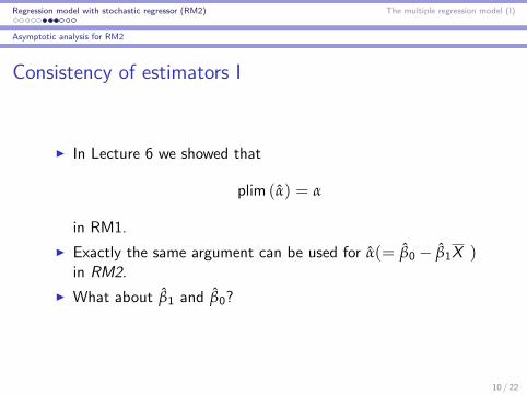
I In Lecture 6 we showed that

plim (α) = α

in RM1.

I Exactly the same argument can be used for α(= β0 − β1X )in RM2.

I What about β1 and β0?

10 / 22



Consistency of estimators II

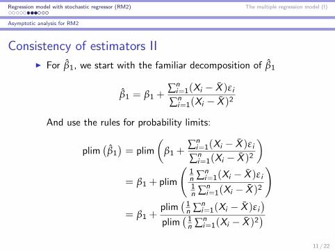
I For β1, we start with the familiar decomposition of β1

β1 = β1 +∑n

i=1(Xi − X )ε i

∑ni=1(Xi − X )2

And use the rules for probability limits:

plim(

β1

)= plim

(β1 +

∑ni=1(Xi − X )ε i

∑ni=1(Xi − X )2

)= β1 + plim

(1n ∑n

i=1(Xi − X )ε i1n ∑n

i=1(Xi − X )2

)

= β1 +plim

(1n ∑n

i=1(Xi − X )ε i)

plim(

1n ∑n

i=1(Xi − X )2)

11 / 22



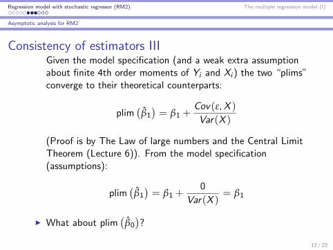
Consistency of estimators IIIGiven the model specification (and a weak extra assumptionabout finite 4th order moments of Yi and Xi ) the two “plims”converge to their theoretical counterparts:

plim(

β1

)= β1 +

Cov(ε,X )

Var(X )

(Proof is by The Law of large numbers and the Central LimitTheorem (Lecture 6)). From the model specification(assumptions):

plim(

β1

)= β1 +

0

Var(X )= β1

I What about plim(

β0

)?

12 / 22



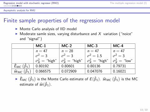
Finite sample properties of the regression modelI Monte Carlo analysis of IID modelI Moderate samle sizes, varying disturbance and X variation (“noice”

and “signal”)

MC-1 MC-2 MC-3 MC-4n = 47 n = 28 n = 47 n = 47σ2 = 3 σ2 = 3 σ2 = 1.5 σ2 = 3σ2X = “high” σ2

X = “high” σ2X = “high” σ2

X = “low”

EMC

(β1

)0.80192 0.80601 0.80136 0.79731

seMC

(β1

)0.066575 0.072909 0.047076 0.16021

I EMC

(β1

)is the Monte Carlo estimate of E (β1). seMC

(β1

)is the MC

estimate of se(β1).

13 / 22



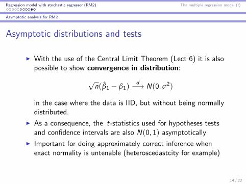
Asymptotic distributions and tests

I With the use of the Central Limit Theorem (Lect 6) it is alsopossible to show convergence in distribution:

√n(β1 − β1)

d−→ N(0, σ2)

in the case where the data is IID, but without being normallydistributed.

I As a consequence, the t-statistics used for hypotheses testsand confidence intervals are also N(0, 1) asymptotically

I Important for doing approximately correct inference whenexact normality is untenable (heteroscedastcity for example)

14 / 22



Summary of summaryI All the properties for the OLS estimators, and the inference theory hold

in the regression model with random regressorI The gap between RM1 and RM2 has now been bridged, and we do not

need the distinction any longer.I In applied modelling we are free to use deterministic and random

explanatory variables, and to combine them in multiple regressionmodels.

I The main bridge principles are conditional expectation and IIDsampling. Later in the course we will return to both and ask newquestions. For example: “What, remains of all the nice OLS propertiesif the variables are not independent?”

I But first we will develop the multivariate regression model under theIID assumption

15 / 22


References: I

I HGL Chapter 5 and 6

I BN Kap 7

16 / 22


Motivation for multivariate regression I

I Economic variables are influenced by several factors, ratherthan one single “primary causal factor”

I Economic theory often imply multivariate models

I In order to test competing theories with the aid of regression,must allow for at least two explanatory variables (bivariate)

I Even if there is only one explanatory variable, the use of apolynomials to model a non-linear relationship, e.g.,

E (Y | Xi ) = β0 + β1Xi + β2X2i

leads to regression models with two regressors

17 / 22


Motivation for multivariate regression II

I Although multiple regression indicates that we will want touse models where the number of regressors is large (k), all thenew theoretical points can be understood with the use of thebivariate model (k = 2).

18 / 22


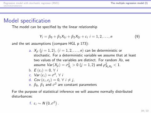
Model specificationThe model can be specified by the linear relationship

Yi = β0 + β1X1i + β2X2i + ε i i = 1, 2, . . . , n (9)

and the set assumptions (compare HGL p 173):

a. Xji (j = 1, 2), (i = 1, 2, . . . , n) can be deterministic orstochastic. For a deterministic variable we assume that at leasttwo values of the variables are distinct. For random Xs, weassume Var(Xji ) = σ2

Xj> 0 (j = 1, 2) and ρ2

X1X2< 1.

b. E (ε i ) = 0, ∀ ic. Var (ε i ) = σ2, ∀ id. Cov (ε i , εj ) = 0, ∀ i 6= j ,e. β0, β1 and σ2 are constant parameters

For the purpose of statistical inference we will assume normally distributeddisturbances:

f. ε i ∼ N(0, σ2

).

19 / 22


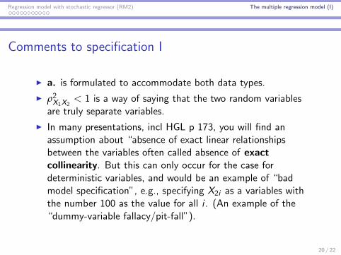
Comments to specification I

I a. is formulated to accommodate both data types.

I ρ2X1X2

< 1 is a way of saying that the two random variablesare truly separate variables.

I In many presentations, incl HGL p 173, you will find anassumption about “absence of exact linear relationshipsbetween the variables often called absence of exactcollinearity. But this can only occur for the case fordeterministic variables, and would be an example of “badmodel specification”, e.g., specifying X2i as a variables withthe number 100 as the value for all i . (An example of the“dummy-variable fallacy/pit-fall”).

20 / 22


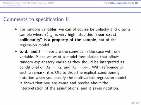
Comments to specification II

I For random variables, we can of course be unlucky and draw asample where r2

X1X2is very high. But this “near exact

collinearity” is a property of the sample, not of theregression model

I b.-d. and f. These are the same as in the case with onevariable. Since we want a model formulation that allowsrandom explanatory variables they should be interpreted asconditional on X1i = x1i and X2i = x21. With reference tosuch a remark, it is OK to drop the explicit conditioningnotation when you specify the multivariate regression model.It shows that you are aware and precise about theinterpretation of the assumptions, and it saves notation.

21 / 22


OLS estimationNothing new here. Chose the estimates that minimize

S(β0,β2,β1) =n

∑i=1

(Yi − β0 − β1X1i − β2X2i )2 (10)

or, equivalently.

S(α,β2,β1) =n

∑i=1

(Yi − α− β1(X1i − X 1)− β2(X2i − X 2))2

whereα := β0 + β1X 1 + β2X 2

I Rest of derivation and examples in class

22 / 22

The regression model with one stochastic regressor ...

Documents