Astronomy & Astrophysics manuscript no. GEVpaper c ESO 2014 February 20, 2014 The RAVE survey: the Galactic escape speed and the mass of the Milky Way T. Piffl 1, 2? , C. Scannapieco 1 , J. Binney 2 , M. Steinmetz 1 , R.-D. Scholz 1 , M. E. K. Williams 1 , R. S. de Jong 1 , G. Kordopatis 3 , G. Matijeviˇ c 4 , O. Bienaymé 5 , J. Bland-Hawthorn 6 , C. Boeche 7 , K. Freeman 8 , B. Gibson 9 , G. Gilmore 3 , E. K. Grebel 7 , A. Helmi 10 , U. Munari 11 , J. F. Navarro 12 , Q. Parker 13, 14, 15 , W. A. Reid 13, 14 , G. Seabroke 16 , F. Watson 17 , R. F. G. Wyse 18 , and T. Zwitter 19, 20 1 Leibniz-Institut für Astrophysik Potsdam (AIP), An der Sternwarte 16, 14482 Potsdam, Germany 2 Rudolf Peierls Centre for Theoretical Physics, 1 Keble Road, Oxford OX1 3NP, UK 3 Institute for Astronomy, University of Cambridge, Madingley Road, Cambridge CB3 0HA, UK 4 Dept. of Astronomy and Astrophysics, Villanova University, 800 E Lancaster Ave, Villanova, PA 19085, USA 5 Observatoire astronomique de Strasbourg, Université de Strasbourg, CNRS, UMR 7550, 11 rue de l’Universié, F-67000 Stras- bourg, France 6 Sydney Institute for Astronomy, University of Sydney, School of Physics A28, NSW 2088, Australia 7 Astronomisches Rechen-Institut, Zentrum für Astronomie der Universität Heidelberg, Mönchhofstr. 12–14, 69120 Heidelberg, Germany 8 Research School of Astronomy and Astrophysics, Australian National University, Cotter Rd., Weston, ACT 2611, Australia 9 Jeremiah Horrocks Institute, University of Central Lancashire, Preston, PR1 2HE, UK 10 Kapteyn Astronomical Institute, University of Groningen, P.O. Box 800, 9700 AV Groningen, The Netherlands 11 National Institute of Astrophysics INAF, Astronomical Observatory of Padova, 36012 Asiago, Italy 12 Senior CIfAR Fellow, University of Victoria, Victoria BC, Canada V8P 5C2 13 Department of Physics, Macquarie University, Sydney, NSW 2109, Australian 14 Research Centre for Astronomy, Astrophysics and Astrophotonics, Macquarie University, Sydney, NSW 2109 Australia 15 Australian Astronomical Observatory, PO Box 296, Epping, NSW 1710, Australia 16 Mullard Space Science Laboratory, University College London, Holmbury St Mary, Dorking, RH5 6NT, UK 17 Australian Astronomical Observatory, PO Box 915, North Ryde, NSW 1670, Australia 18 Department of Physics & Astronomy, Johns Hopkins University, Baltimore, MD 21218, USA 19 University of Ljubljana, Faculty of Mathematics and Physics, Jadranska 19, Ljubljana, Slovenia 20 Center of excellence space-si, Askerceva 12, Ljubljana, Slovenia Received ???; Accepted ??? ABSTRACT We construct new estimates on the Galactic escape speed at various Galactocentric radii using the latest data release of the Radial Velocity Experiment (RAVE DR4). Compared to previous studies we have a database larger by a factor of 10 as well as reliable distance estimates for almost all stars. Our analysis is based on the statistical analysis of a rigorously selected sample of 90 high- velocity halo stars from RAVE and a previously published data set. We calibrate and extensively test our method using a suite of cosmological simulations of the formation of Milky Way-sized galaxies. Our best estimate of the local Galactic escape speed, which we define as the minimum speed required to reach three virial radii R 340 , is 533 +54 -41 km s -1 (90% confidence) with an additional 4% systematic uncertainty, where R 340 is the Galactocentric radius encompassing a mean overdensity of 340 times the critical density for closure in the Universe. From the escape speed we further derive estimates of the mass of the Galaxy using a simple mass model with two options for the mass profile of the dark matter halo: an unaltered and an adiabatically contracted Navarro, Frenk & White (NFW) sphere. If we fix the local circular velocity the latter profile yields a significantly higher mass than the uncontracted halo, but if we instead use the statistics on halo concentration parameters in large cosmological simulations as a constraint, we find very similar masses for both models. Our best estimate for M 340 , the mass interior to R 340 (dark matter and baryons), is 1.3 +0.4 -0.3 × 10 12 M (corresponding to M 200 = 1.6 +0.5 -0.4 × 10 12 M ). This estimate is in good agreement with recently published independent mass estimates based on the kinematics of more distant halo stars and the satellite galaxy Leo I. Key words. Galaxy: fundamental parameters – Galaxy: kinematics and dynamics – Galaxy: halo 1. Introduction In the recent years quite a large number of studies concerning the mass of our Galaxy were published. This parameter is of partic- ular interest, because it provides a test for the current cold dark matter paradigm. There is now convincing evidence (e.g. Smith ? email: [email protected] et al. 2007) that the Milky Way (MW) exhibits a similar discrep- ancy between luminous and dynamical mass estimates as was already found in the 1970’s for other galaxies. A robust mea- surement of this parameter is needed to place the Milky Way in the cosmological framework. Furthermore, a detailed knowl- edge of the mass and the mass profile of the Galaxy is crucial for understanding and modeling the dynamic evolution of the MW Article number, page 1 of 16 arXiv:1309.4293v3 [astro-ph.GA] 13 Nov 2013

Welcome message from author
This document is posted to help you gain knowledge. Please leave a comment to let me know what you think about it! Share it to your friends and learn new things together.
Transcript

Astronomy & Astrophysics manuscript no. GEVpaper c©ESO 2014February 20, 2014
The RAVE survey: the Galactic escape speed and the mass of theMilky Way
T. Piffl1, 2?, C. Scannapieco1, J. Binney2, M. Steinmetz1, R.-D. Scholz1, M. E. K. Williams1, R. S. de Jong1,G. Kordopatis3, G. Matijevic4, O. Bienaymé5, J. Bland-Hawthorn6, C. Boeche7, K. Freeman8, B. Gibson9,G. Gilmore3, E. K. Grebel7, A. Helmi10, U. Munari11, J. F. Navarro12, Q. Parker13, 14, 15, W. A. Reid13, 14,
G. Seabroke16, F. Watson17, R. F. G. Wyse18, and T. Zwitter19, 20
1 Leibniz-Institut für Astrophysik Potsdam (AIP), An der Sternwarte 16, 14482 Potsdam, Germany2 Rudolf Peierls Centre for Theoretical Physics, 1 Keble Road, Oxford OX1 3NP, UK3 Institute for Astronomy, University of Cambridge, Madingley Road, Cambridge CB3 0HA, UK4 Dept. of Astronomy and Astrophysics, Villanova University, 800 E Lancaster Ave, Villanova, PA 19085, USA5 Observatoire astronomique de Strasbourg, Université de Strasbourg, CNRS, UMR 7550, 11 rue de l’Universié, F-67000 Stras-
bourg, France6 Sydney Institute for Astronomy, University of Sydney, School of Physics A28, NSW 2088, Australia7 Astronomisches Rechen-Institut, Zentrum für Astronomie der Universität Heidelberg, Mönchhofstr. 12–14, 69120 Heidelberg,
Germany8 Research School of Astronomy and Astrophysics, Australian National University, Cotter Rd., Weston, ACT 2611, Australia9 Jeremiah Horrocks Institute, University of Central Lancashire, Preston, PR1 2HE, UK
10 Kapteyn Astronomical Institute, University of Groningen, P.O. Box 800, 9700 AV Groningen, The Netherlands11 National Institute of Astrophysics INAF, Astronomical Observatory of Padova, 36012 Asiago, Italy12 Senior CIfAR Fellow, University of Victoria, Victoria BC, Canada V8P 5C213 Department of Physics, Macquarie University, Sydney, NSW 2109, Australian14 Research Centre for Astronomy, Astrophysics and Astrophotonics, Macquarie University, Sydney, NSW 2109 Australia15 Australian Astronomical Observatory, PO Box 296, Epping, NSW 1710, Australia16 Mullard Space Science Laboratory, University College London, Holmbury St Mary, Dorking, RH5 6NT, UK17 Australian Astronomical Observatory, PO Box 915, North Ryde, NSW 1670, Australia18 Department of Physics & Astronomy, Johns Hopkins University, Baltimore, MD 21218, USA19 University of Ljubljana, Faculty of Mathematics and Physics, Jadranska 19, Ljubljana, Slovenia20 Center of excellence space-si, Askerceva 12, Ljubljana, Slovenia
Received ???; Accepted ???
ABSTRACT
We construct new estimates on the Galactic escape speed at various Galactocentric radii using the latest data release of the RadialVelocity Experiment (RAVE DR4). Compared to previous studies we have a database larger by a factor of 10 as well as reliabledistance estimates for almost all stars. Our analysis is based on the statistical analysis of a rigorously selected sample of 90 high-velocity halo stars from RAVE and a previously published data set. We calibrate and extensively test our method using a suite ofcosmological simulations of the formation of Milky Way-sized galaxies. Our best estimate of the local Galactic escape speed, whichwe define as the minimum speed required to reach three virial radii R340, is 533+54
−41 km s−1 (90% confidence) with an additional 4%systematic uncertainty, where R340 is the Galactocentric radius encompassing a mean overdensity of 340 times the critical density forclosure in the Universe. From the escape speed we further derive estimates of the mass of the Galaxy using a simple mass modelwith two options for the mass profile of the dark matter halo: an unaltered and an adiabatically contracted Navarro, Frenk & White(NFW) sphere. If we fix the local circular velocity the latter profile yields a significantly higher mass than the uncontracted halo,but if we instead use the statistics on halo concentration parameters in large cosmological simulations as a constraint, we find verysimilar masses for both models. Our best estimate for M340, the mass interior to R340 (dark matter and baryons), is 1.3+0.4
−0.3 × 10¹² M(corresponding to M200 = 1.6+0.5
−0.4 × 10¹² M). This estimate is in good agreement with recently published independent mass estimatesbased on the kinematics of more distant halo stars and the satellite galaxy Leo I.
Key words. Galaxy: fundamental parameters – Galaxy: kinematics and dynamics – Galaxy: halo
1. Introduction
In the recent years quite a large number of studies concerning themass of our Galaxy were published. This parameter is of partic-ular interest, because it provides a test for the current cold darkmatter paradigm. There is now convincing evidence (e.g. Smith
? email: [email protected]
et al. 2007) that the Milky Way (MW) exhibits a similar discrep-ancy between luminous and dynamical mass estimates as wasalready found in the 1970’s for other galaxies. A robust mea-surement of this parameter is needed to place the Milky Wayin the cosmological framework. Furthermore, a detailed knowl-edge of the mass and the mass profile of the Galaxy is crucial forunderstanding and modeling the dynamic evolution of the MW
Article number, page 1 of 16
arX
iv:1
309.
4293
v3 [
astr
o-ph
.GA
] 1
3 N
ov 2
013

satellite galaxies (e.g. Kallivayalil et al. (2013) for the Magel-lanic clouds) and the Local Group (van der Marel et al. 2012b,a).Generally, it can be observed, that mass estimates based on stel-lar kinematics yield low values <∼ 1012 M (Smith et al. 2007;Xue et al. 2008; Kafle et al. 2012; Deason et al. 2012; Bovyet al. 2012), while methods exploiting the kinematics of satellitegalaxies or statistics of large cosmological dark matter simula-tions find larger values (Wilkinson & Evans 1999; Li & White2008; Boylan-Kolchin et al. 2011; Busha et al. 2011; Boylan-Kolchin et al. 2013). There are some exceptions, however.For example, Przybilla et al. (2010) find a rather high value of1.7× 1012 M taking into account the star J1539+0239, a hyper-velocity star approaching the MW and Gnedin et al. (2010) find asimilar value using Jeans modeling of a stellar population in theouter halo. On the other hand Vera-Ciro et al. (2013) estimatea most likely MW mass of 0.8 × 10¹² M analyzing the Aquar-ius simulations (Springel et al. 2008) in combination with semi-analytic models of galaxy formation. Watkins et al. (2010) reportan only slightly higher value based on the line of sight veloci-ties of satellite galaxies (see also Sales et al. (2007)), but whenthey include proper motion estimates they again find a highermass of 1.4 × 10¹² M. Using a mixture of stars and satellitegalaxies Battaglia et al. (2005, 2006) also favor a low mass be-low 1012 M. McMillan (2011) found an intermediate mass of1.3 × 1012 M including also constraints from photometric data.A further complication of the matter comes from the definitionof the total mass of the Galaxy which is different for differentauthors and so a direct comparison of the quoted values has tobe done with care. Finally, there is an independent strong upperlimit for the Milky Way mass coming from Local Group timingarguments that estimate the total mass of the combined mass ofthe Milky Way and Andromeda to 3.2 ± 0.6 × 10¹² M (van derMarel et al. 2012b).In this work we attempt to estimate the mass of the MW throughmeasuring the escape speed at several Galactocentric radii. Inthis we follow up on the studies by Leonard & Tremaine (1990),Kochanek (1996) and Smith et al. (2007) (S07, hereafter). Thelatter work made use of an early version of the Radial VelocityExperiment (RAVE; Steinmetz et al. (2006)), a massive spectro-scopic stellar survey that finished its observational phase in April2013 and the almost complete set of data will soon be publiclyavailable in the fourth data release (Kordopatis et al. 2013). Thistremendous data set forms the foundation of our study.The escape speed measures the depth of the potential well of theMilky Way and therefore contains information about the massdistribution exterior to the radius for which it is estimated. Itthus constitutes a local measurement connected to the very out-skirts of our Galaxy. In the absence of dark matter and a purelyNewtonian gravity law we would expect a local escape speedof√
2VLSR = 311 km s−1, assuming the local standard of rest,VLSR to be 220 km s−1 and neglecting the small fraction of visi-ble mass outside the solar circle (Fich & Tremaine 1991). How-ever, the estimates in the literature are much larger than thisvalue, starting with a minimum value of 400 km s−1 (Alexander1982) to the currently most precise measurement by S07 whofind [498,608] km s−1 as 90% confidence range.The paper is structured as follows: in Section 2 we introduce thebasic principles of our analysis. Then we go on (Section 3) todescribe how we use cosmological simulations to obtain a priorfor our maximum likelihood analysis and thereby calibrate ourmethod. After presenting our data and the selection process inSection 4 we obtain estimates on the Galactic escape speed inSection 5. The results are extensively discussed in Section 6and mass estimates for our Galaxy are obtained and compared to
previous measurements. Finally, we conclude and summarize inSection 7.
2. Methodology
The basic analysis strategy applied in this study was initially in-troduced by Leonard & Tremaine (1990) and later extended byS07. They assumed that the stellar system could be described byan ergodic distribution function (DF) f (E) that satisfied f → 0as E → Φ, the local value of the gravitational potential Φ(r).Then the density of stars in velocity space will be a function n(3)of speed 3 and tend to zero as 3 → 3esc = (2Φ)1/2. Leonard &Tremaine (1990) proposed that the asymptotic behavior of n(3)could be modeled as
n(3) ∝ (3esc − 3)k, (1)
for 3 < 3esc, where k is a parameter. Hence we should be able toobtain an estimate of 3esc from a local sample of stellar velocities.S07 used a slightly different functional form
n(3) ∝ (32esc − 32)k = (3esc − 3)k(3esc + 3)k, (2)
that can be derived if f (E) ∝ Ek is assumed, but, as we will seein Section 3, results from cosmological simulations are betterapproximated by Eq. 1.Currently, the most accurate velocity measurements are line-of-sight velocities, 3los, obtained from spectroscopy via the Dopplereffect. These measurements have typically uncertainties of a fewkm s−1, which is an order of magnitude smaller than the typicaluncertainties on tangential velocities obtained from proper mo-tions currently available. Leonard & Tremaine (1990) alreadyshowed with simulated data, that because of this, estimates fromradial velocities alone are as accurate as estimates that use propermotions as well. The measured velocities 3los have to be cor-rected for the solar motion to enter a Galactocentric rest frame.These corrected velocities we denote with 3‖.Following Leonard & Tremaine (1990) we can infer the distri-bution of 3‖ by integrating over all perpendicular directions:
n‖(3‖ | r, k) ∝
∫dv n(v | r, k)δ(3‖ − v · m)
∝(3esc(r) − |3‖|
)k+1 (3)
again for |3‖| < 3esc. Here δ denotes the Dirac delta function andm represents a unit vector along the line of sight.We do not expect that our approximation for the velocity DFis valid over the whole range of velocities, but only at the highvelocity tail of the distribution. Hence we impose a lower limit3min for the stellar velocities. A further important requirementis that the stellar velocities come from a population that is notrotationally supported, because such a population is clearly notdescribed by an ergodic DF. In the case of stars in the Galaxy,this means that we have to select for stars of the Galactic stellarhalo component.We now apply the following approach to the estimation of 3esc.We adopt the likelihood function
L(3‖) =(3esc − |3‖|)k+1∫ 3esc
3mind3 (3esc − |3‖|)k+1
= (k + 2)(3esc − |3‖|)k+1
(3esc − 3min)k+2 (4)
and determine the likelihood of our catalog of stars that have|3‖| > 3min for various choices of 3esc and k, then we marginalizethe likelihood over the nuisance parameter k and determine thetrue value of 3esc as the speed that maximizes the marginalizedlikelihood.
Article number, page 2 of 16
T. Piffl et al.: The RAVE survey: the Galactic escape speed and the mass of the Milky Way
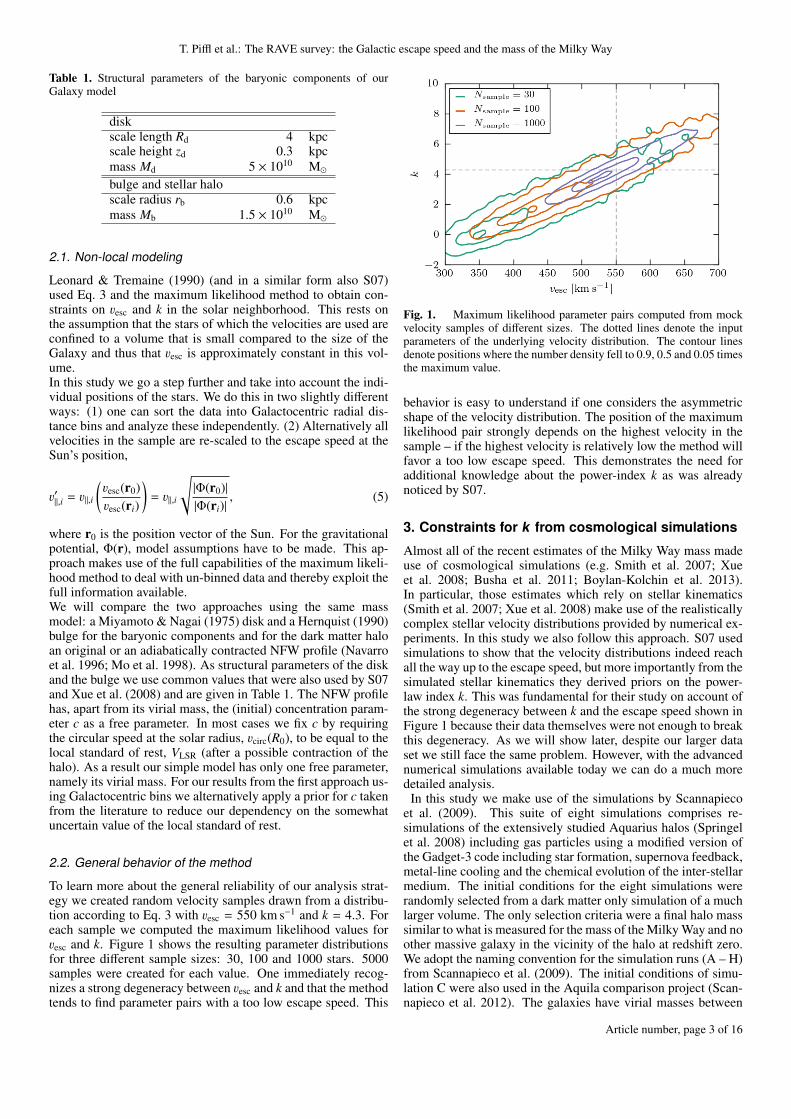
Table 1. Structural parameters of the baryonic components of ourGalaxy model
diskscale length Rd 4 kpcscale height zd 0.3 kpcmass Md 5 × 10¹⁰ Mbulge and stellar haloscale radius rb 0.6 kpcmass Mb 1.5 × 10¹⁰ M
2.1. Non-local modeling
Leonard & Tremaine (1990) (and in a similar form also S07)used Eq. 3 and the maximum likelihood method to obtain con-straints on 3esc and k in the solar neighborhood. This rests onthe assumption that the stars of which the velocities are used areconfined to a volume that is small compared to the size of theGalaxy and thus that 3esc is approximately constant in this vol-ume.In this study we go a step further and take into account the indi-vidual positions of the stars. We do this in two slightly differentways: (1) one can sort the data into Galactocentric radial dis-tance bins and analyze these independently. (2) Alternatively allvelocities in the sample are re-scaled to the escape speed at theSun’s position,
3′‖,i = 3‖,i
(3esc(r0)3esc(ri)
)= 3‖,i
√|Φ(r0)||Φ(ri)|
, (5)
where r0 is the position vector of the Sun. For the gravitationalpotential, Φ(r), model assumptions have to be made. This ap-proach makes use of the full capabilities of the maximum likeli-hood method to deal with un-binned data and thereby exploit thefull information available.We will compare the two approaches using the same massmodel: a Miyamoto & Nagai (1975) disk and a Hernquist (1990)bulge for the baryonic components and for the dark matter haloan original or an adiabatically contracted NFW profile (Navarroet al. 1996; Mo et al. 1998). As structural parameters of the diskand the bulge we use common values that were also used by S07and Xue et al. (2008) and are given in Table 1. The NFW profilehas, apart from its virial mass, the (initial) concentration param-eter c as a free parameter. In most cases we fix c by requiringthe circular speed at the solar radius, 3circ(R0), to be equal to thelocal standard of rest, VLSR (after a possible contraction of thehalo). As a result our simple model has only one free parameter,namely its virial mass. For our results from the first approach us-ing Galactocentric bins we alternatively apply a prior for c takenfrom the literature to reduce our dependency on the somewhatuncertain value of the local standard of rest.
2.2. General behavior of the method
To learn more about the general reliability of our analysis strat-egy we created random velocity samples drawn from a distribu-tion according to Eq. 3 with 3esc = 550 km s−1 and k = 4.3. Foreach sample we computed the maximum likelihood values for3esc and k. Figure 1 shows the resulting parameter distributionsfor three different sample sizes: 30, 100 and 1000 stars. 5000samples were created for each value. One immediately recog-nizes a strong degeneracy between 3esc and k and that the methodtends to find parameter pairs with a too low escape speed. This
Fig. 1. Maximum likelihood parameter pairs computed from mockvelocity samples of different sizes. The dotted lines denote the inputparameters of the underlying velocity distribution. The contour linesdenote positions where the number density fell to 0.9, 0.5 and 0.05 timesthe maximum value.
behavior is easy to understand if one considers the asymmetricshape of the velocity distribution. The position of the maximumlikelihood pair strongly depends on the highest velocity in thesample – if the highest velocity is relatively low the method willfavor a too low escape speed. This demonstrates the need foradditional knowledge about the power-index k as was alreadynoticed by S07.
3. Constraints for k from cosmological simulations
Almost all of the recent estimates of the Milky Way mass madeuse of cosmological simulations (e.g. Smith et al. 2007; Xueet al. 2008; Busha et al. 2011; Boylan-Kolchin et al. 2013).In particular, those estimates which rely on stellar kinematics(Smith et al. 2007; Xue et al. 2008) make use of the realisticallycomplex stellar velocity distributions provided by numerical ex-periments. In this study we also follow this approach. S07 usedsimulations to show that the velocity distributions indeed reachall the way up to the escape speed, but more importantly from thesimulated stellar kinematics they derived priors on the power-law index k. This was fundamental for their study on account ofthe strong degeneracy between k and the escape speed shown inFigure 1 because their data themselves were not enough to breakthis degeneracy. As we will show later, despite our larger dataset we still face the same problem. However, with the advancednumerical simulations available today we can do a much moredetailed analysis.
In this study we make use of the simulations by Scannapiecoet al. (2009). This suite of eight simulations comprises re-simulations of the extensively studied Aquarius halos (Springelet al. 2008) including gas particles using a modified version ofthe Gadget-3 code including star formation, supernova feedback,metal-line cooling and the chemical evolution of the inter-stellarmedium. The initial conditions for the eight simulations wererandomly selected from a dark matter only simulation of a muchlarger volume. The only selection criteria were a final halo masssimilar to what is measured for the mass of the Milky Way and noother massive galaxy in the vicinity of the halo at redshift zero.We adopt the naming convention for the simulation runs (A – H)from Scannapieco et al. (2009). The initial conditions of simu-lation C were also used in the Aquila comparison project (Scan-napieco et al. 2012). The galaxies have virial masses between
Article number, page 3 of 16

Table 2. Virial radii, masses and velocities after re-scaling the sim-ulations to have a circular speed of 220 km s−1 at the solar radiusR0 = 8.28 kpc.
Simulation R340 M340 V340 scaling factor(kpc) (1010 M) (km s−1)
A 154 77 147 1.20B 179 120 170 0.82C 157 81 149 1.22D 176 116 168 1.05E 155 79 148 1.07F 166 96 158 0.94G 165 94 157 0.88H 143 62 137 1.02
0.7−1.6×10¹²M and span a large range of morphologies, fromgalaxies with a significant disk component (e.g. simulations Cand G) to pure elliptical galaxies (simulation F). The mass res-olution is 0.22 – 0.56 × 10⁶ M. For a detailed description ofthe simulations we refer the reader to Scannapieco et al. (2009,2010, 2011). Details regarding the simulation code can be foundin Scannapieco et al. (2005, 2006) and also in Springel (2005).An important aspect of the Scannapieco et al. (2009) sample isthat the eight simulated galaxies have a broad variety of mergerand accretion histories, providing a more or less representativesample of Milky Way-mass galaxies formed in a ΛCDM uni-verse (Scannapieco et al. 2011). Our set of simulations is thususeful for the present study, since it gives us information on theevolution of various galaxies, including all the necessary cosmo-logical processes acting during the formation of galaxies, and ata relatively high resolution.Also, we note that the same code has been successfully appliedto the study of dwarf galaxies (Sawala et al. 2011, 2012), us-ing the same set of input parameters. Despite a mismatch in thebaryon fraction (which is common to almost all simulations ofthis kind), the resulting galaxies exhibited structures and stellarpopulations consistent with observations, proving that the codeis able to reproduce the formation of galaxies of different massesin a consistent way. Taking into account that the outer stellarhalo of massive galaxies form from smaller accreted galaxies,the fact that we do not need to fine-tune the code differently fordifferent masses proves once more the reliability of the simula-tion code and its results.To allow a better comparison to the Milky Way we re-scalethe simulations to have a circular speed at the solar radius,R0 = 8.28 kpc, of 220 km s−1 by the following transformation:
r′i = ri/ f , v′i = vi/ f ,m′i = mi/ f 3, Φ′i = Φi/ f 2 (6)
with mi and Φi are the mass and the gravitational potential energyof the ith star particle in the simulations. The resulting masses,M340, radii, R340, and velocities, V340 as well as the scaling fac-tors are given in Table 2. Throughout this work we use a Hubbleconstant H = 73 km s−1 Mpc−1 and define the virial radius tocontain a mean matter density 340 ρcrit, where ρcrit = 3H2/8πGis the critical energy density for a closed universe. The abovetransformations do not alter the simulation results as they pre-serve the numerical value of the gravitational constant G gov-erning the stellar motions and also the mass density field ρ(r)that governs the gas motions as well as the numerical star forma-tion recipe. Only the supernova feedback recipe is not scaling inthe same way, but since our scaling factors f are close to unitythis is not a major concern.
Since the galaxies in the simulations are not isolated systems,we have to define a limiting distance above which we considera particle to have escaped its host system. We set this distanceto 3R340 and set the potential to zero at this radius which resultsin distances between 430 and 530 kpc in the simulations. Thischoice is an educated guess and our results are not sensitive tosmall changes, because the gravitational potential changes onlyweakly with radius at these distances and in addition, the result-ing escape speed is only proportional to the square root of thepotential. However, we must not choose a too small value, be-cause otherwise we underestimate the escape speed encoded inthe stellar velocity field. On the other hand, we must cut in aregime where the potential is yet not dominated by neighboring(clusters of) galaxies. Our choice is in addition close to half ofthe distance of the Milky Way and its nearest massive neighbor,the Andromeda galaxy. We further test our choice below. Withthis definition of the cut-off radius we obtain local escape speedsat R0 from the center between 475 and 550 km s−1.Now we select a population of star particles belonging to thestellar halo component. In many numerical studies the separa-tion of the particles into disk and bulge/halo populations is doneusing a circularity parameter which is defined as the ratio be-tween the particle’s angular momentum in the z-direction1 andthe angular momentum of a circular orbit either at the particle’scurrent position (Scannapieco et al. 2009, 2011) or at the par-ticle’s orbital energy (Abadi et al. 2003). A threshold value isthen defined which divides disk and bulge/halo particles. We optfor the very conservative value of 0 which means that we onlytake counter-rotating particles. Practically, this is equivalent toselecting all particles with a positive tangential velocity w.r.t theGalactic center. This choice allows us to do exactly the sameselection as we will do later with the real observational data forwhich we have to use a very conservative value because of thelarger uncertainties in the proper motion measurements.For similar reasons we also keep only particles in our samplethat have Galactocentric distances between 4 and 12 kpc whichreflects the range of values of the stars in the RAVE survey whichwe will use for this study. This further ensures that we excludeparticles belonging to the bulge component.Finally, we set the distance R0 of the observer from the Galac-tic center to be 8.28 kpc and choose an azimuthal position φ0and compute the line-of-sight velocity 3‖,i for each particle in thesample. We further know the exact potential energy Φi of eachparticle and therefore their local escape speed 3esc,i is easily com-puted.We do this for 4 different azimuthal positions separated fromeach other by 90. The positions were chosen such that theinclination angle w.r.t. a possible bar is 45. The correspond-ing samples are analyzed individually and also combined. Note,that these samples are practically statistically independent eventhough a particle could enter two or more samples. However,because we only consider the line-of-sight component of the ve-locities, only in the unlikely case that a particle is located exactlyon the line-of-sight between two observer positions it would gainan incorrect double weight in the combined statistical analysis.Figure 2 shows the velocity-space density of star particles as a
function of 1 − 3‖/3esc and we see that, remarkably, at the high-est speeds these plots have a reasonably straight section, just asLeonard & Tremaine (1990) hypothesized. The slopes of theserectilinear sections scatter around k = 3 as we will see later.We also considered the functional form proposed by S07 for the
1 The coordinate system is defined such that the disk rotates in thex − y-plane.
Article number, page 4 of 16

T. Piffl et al.: The RAVE survey: the Galactic escape speed and the mass of the Milky Way
Fig. 2. Normalized velocity distributions of the stellar halo populationin our eight simulations plotted as a function of 1−3‖/3esc. Only counter-rotating particles that have Galactocentric distances r between 4 and12 kpc are considered to select for halo particles (see Section 3.1) and tomatch the volume observed by the RAVE survey. To allow a comparisoneach velocity was divided by the escape speed at the particle’s position.Different colors indicate different simulations and for each simulationthe 3‖ distribution is shown for four different observer positions. Thetop bundle of curves shows the mean of these four distributions for eachsimulation plotted on top of each other to allow a comparison. Theprofiles are shifted vertically in the plot for better visibility. The graylines illustrate Eq. 3 with power-law index k = 3.
Fig. 3. Same as the top bundle of lines in Figure 2 but plotted as afunction of 1 − 32
‖/32esc. If the data follows the velocity DF proposed by
S07 (gray line) the data should form a straight line in this representation.
Fig. 4. Median values of the likelihood distributions of the power-lawindex k as a function of the applied threshold velocity 3min.
velocity DF, that is n(3) ∝ (32esc− 32)k. Figure 3 tests this DF with
the simulation data. The curvature implies that this DF does notrepresent the simulation data as well as the formula proposed byLeonard & Tremaine (1990).If we fit Eq. 3 to the velocity distributions while fixing k to 3 werecover the escape speeds within 6%. This confirms our choiceof the cut-off radius for the gravitational potential, 3R340, thatwas used during the definition of the escape speeds.
3.1. The velocity threshold
We now try to find the best value for the lower threshold veloc-ity 3min. S07 had to use a high threshold value for their radialvelocities of 300 km s−1, because the threshold had an additionalpurpose, namely to select stars from the non-rotating halo com-ponent. If one can identify these stars by other means the veloc-ity threshold can be lowered significantly. This adds more starsto the sample and thereby puts our analysis on a broader basis.If the stellar halo had the shape of an isotropic Plummer (1911)sphere, the threshold could be set to zero, because for this modelthe S07 verison of our approximated velocity distribution func-tion would be exact. However, for other DFs we need to choosea higher value to avoid regions where our approximation breaksdown. Again, we use the simulations to select an appropriatevalue.We compute the likelihood distribution of k in each simulationusing different velocity thresholds using the likelihood estimator
Ltot(k | 3min) =∏
i
L(3‖,i). (7)
Figure 4 plots the median values of the likelihood distributionsas a function of the threshold velocity. We see a trend of in-creasing k for 3min <∼ 150 km s−1 and roughly random behav-ior above. For low values of 3min simulation G does not followthe general trend. This simulation is the only one in the samplethat has a dominating bar in its center (Scannapieco & Athanas-soula 2012) which could contain counter-rotating stars. Giventhis fact a likely explanation for its peculiar behavior is that witha low velocity threshold, bar particles start entering the sampleand thereby alter the velocity distribution.Simulation E exhibits a dip around 3min ' 300 km s−1. A spa-tially dispersed stellar stream of significant mass is counter-orbiting the galaxy and is entering the sample at one of the ob-
Article number, page 5 of 16
server positions. This is also clearly visible in Figure 2 as a bumpin one of the velocity distributions between 0.2 and 0.3. Further-more, this galaxy has a rapidly rotating spheroidal component(Scannapieco et al. 2009).The galaxy in Simulation C has a satellite galaxy very close by.We exclude all star particles in a radius of 3 kpc around the satel-lite center from our analysis, but there will still be particles enter-ing our samples which originate from this companion and whichdo not follow the general velocity DF.All three cases are unlikely to apply for our Milky Way. Ourgalaxy hosts a much shorter bar and up to now no signatures ofa massive stellar stream were found in the RAVE data (Seabrokeet al. 2008; Williams et al. 2011; Antoja et al. 2012). However,it is very interesting to see how our method performs in theserather extreme cases.We adopt threshold velocities 3min = 200 km s−1 and 300 km s−1.Both are far enough from the regime where we see systematicevolution in the k values (3min ≤ 150 km s−1). For the highervalue we can drop the criterion for the particles to be counter-rotating because we can expect the contamination by disk starsto be negligible (S07) and thus partly compensate for the reducedsample size.
3.1.1. An optimal prior for k
From Figure 4 it seems clear that the different simulated galaxiesdo not share exactly the same k, but cover a considerable rangeof values. Thus in the analysis of the real data we will have toconsider this whole range. We fix the extent of this range byrequiring that it delivers optimal results for all four observer po-sitions in all eight simulated galaxies. Hence we applied ouranalysis to the simulated data by computing the posterior proba-bility distribution
p(3esc) ∝∫ kmax
kmin
dk∏
i
L(3′‖,i | 3esc, k), (8)
where L was defined in Eq. 4 and 3′‖,i is the ith re-scaled line-
of-sight velocity as defined in Eq. 5. We define the median ofp(3esc), 3esc, as the best estimate. For a comparison of the esti-mates between different simulations we consider the normalizedestimate 3esc = 3esc/3esc,true with 3esc,true being the true local es-cape speed in the simulation. By varying kmin and kmax we iden-tify those values that minimize the scatter in the sample of 323esc values and at the same time leave the median of the sampleclose to unity. We find very similar intervals for both thresholdvelocities and adopt the interval
2.3 < k < 3.7 . (9)
Reassuringly, this is very close to the lower part of the intervalfound by S07 (2.7 – 4.7) using a different set of simulations.The scatter of the 3esc〉 values is smaller than 3.5% (1σ) for bothvelocity thresholds. This scatter cannot be completely explainedby the statistical uncertainties of the estimates, so there seems tobe an additional uncertainty intrinsic to our analysis techniqueitself. We will try to quantify this in the next section.
3.1.2. Realistic tests
One important test for our method is whether it still yieldscorrect results if we have imperfect data and a non-isotropicdistribution of lines of sights. To simulate typical RAVEmeasurement errors we attached random Gaussian errors on
Fig. 5. Distribution of 3esc resulting from our 32 test runs of our anal-ysis on simulation data equipped with RAVE-like observational errorsand observed in a RAVE-like sky region. In each of the eight simula-tions four different azimuthal observer positions were tested. A valueof unity means an exact recovery of the true local escape speed. Thetwo histograms correspond to our two velocity thresholds applied to thedata.
the parallaxes (distance−1), radial velocities and the two propermotion values with standard deviations of 30%, 3 km s−1 and2 mas, respectively. We computed the angular positions of eachparticle (for a given observer position) and selected only thoseparticles which fell into the approximate survey geometry of theRAVE survey. The latter we define by declination δ < 0 andgalactic latitude |b| > 15.Figure 5 shows the resulting distributions of 3esc for the twovelocity thresholds. Again, the width of the distributions cannotbe soly explained by the statistical uncertainties computed fromthe likelihood distribution, but an additional uncertainty of ' 4%is required to explain the data in a Gaussian approximation. Thedistribution for 3min = 300 km s−1 in addition exhibits a shift tohigher values by ' 3%. Due to the low number statistics thesignificance of the shift is unclear (∼ 3σ). As we will see inSection 5, compared to the statistical uncertainties arising whenwe analyse the real data it would presents a minor contributionto the overall uncertainty and we neglect the shift for this study.
We can go a step further and try to recover the masses of thesimulated galaxies using the escape speed estimates. To do thiswe use the original mass profile of the baryonic componentsof the galaxies to model our knowledge about the visual partsof the Galaxy and impose an analytic expression for the darkmatter halo. As we will do for the real analysis we try twomodels: an unaltered and an adiabatically contracted NFWsphere. We adjust the halo parameters, the virial mass M340and the concentration c, to match both boundary conditions,the circular speed and the escape speed at the solar radius.Figure 6 plots the ratios of the estimated masses and thereal virial masses taken from the simulations directly. Theadiabatically contracted halo on average over-estimates thevirial mass by 25%, while the pure NFW halo systematicallyunderstates the mass by about 15%. For both halo models wefind examples which obtain a very good match with the realmass (e.g. simulation B for the contracted halo and simulationH for the pure NFW halo). However, the cases where thecontracted halo yields better results coincide with those caseswhere the escape speed was underestimated. The coloredsymbols in Figure 6 mark the mass estimates obtained using theexact escape speed computed from the gravitational potential
Article number, page 6 of 16

T. Piffl et al.: The RAVE survey: the Galactic escape speed and the mass of the Milky Way
Fig. 6. Ratios of the estimated and real virial masses in the eightsimulations. For each simulation four mass estimates are plotted basedon four azimuthal positions of the Sun in the galaxy. The symbols witherror-bars represent the estimates based on the median velocities 3escobtained from the error-prone simulation data, while the black symbolsshow mass estimates for which the real escape speed was used as aninput.
in the simulation directly. This reveals that the mass estimatesfrom the two halo models effectively bracket the real mass asexpected. Note, that we also recover the masses of the threesimulations C, E and G that show peculiarities in their velocitydistributions. Only for simulation E and one azimuthal observerposition do we completely fail to recover the mass. In this casethere is a prominent stellar stream moving along the line of sight.
4. Data
4.1. The RAVE survey
The major observational data for this study comes from thefourth data release (DR4) of Radial Velocity Experiment(RAVE), a massive spectroscopic stellar survey conducted us-ing the 6dF multi-object spectrograph on the 1.2-m UK SchmidtTelescope at the Siding Springs Observatory (Australia). A gen-eral description of the project can be found in the data releasepapers: Steinmetz et al. (2006); Zwitter et al. (2008); Siebertet al. (2011); Kordopatis et al. (2013). The spectra are measuredin the Ca ii triplet region with a resolution of R = 7000. In or-der to provide an unbiased velocity sample the survey selectionfunction was kept as simple as possible: it is magnitude limited(9 < I < 12) and has a weak color-cut of J − Ks > 0.5 for starsnear the Galactic disk and the Bulge.In addition to the very precise line-of-sight velocities, 3los, sev-eral other stellar properties could be derived from the spectra.The astrophysical parameters effective temperature Teff , surfacegravity log g and metallicity [M/H] were multiply estimated us-ing different analysis techniques (Zwitter et al. 2008; Siebertet al. 2011; Kordopatis et al. 2011). Breddels et al. (2010), Zwit-ter et al. (2010), Burnett et al. (2011) and Binney et al. (2013) in-dependently used these estimates to derive spectro-photometricdistances for a large fraction of the stars in the survey. Matije-vic et al. (2012) performed a morphological classification of thespectra and in this way identify binaries and other peculiar stars.Finally Boeche et al. (2011) developed a pipeline to derive indi-vidual chemical abundances from the spectra.The DR4 contains information about nearly 500 000 spectra of
more than 420 000 individual stars. The target catalog was alsocross-matched with other databases to be augmented with ad-ditional information like apparent magnitudes and proper mo-tions. For this study we adopted the distances provided by Bin-ney et al. (2013)2 and the proper motions from the UCAC4 cat-alog (Zacharias et al. 2013).
4.2. Sample selection
The wealth of information in the RAVE survey presents an idealfoundation for our study. Since S07 the amount of availablespectra has grown by a factor of 10 and stellar parameters havebecome available. The number of high-velocity stars has unfor-tunately not increased by the same factor, which is most likelydue to the fact that RAVE concentrated more on lower Galacticlatitudes where the relative abundance of halo stars – which canhave these high velocities – is much lower.We use only high-quality observations by selecting only starswhich fulfill the following criteria:
– the stars must be classified as ’normal’ according to the clas-sification by Matijevic et al. (2012),
– the Tonry-Davis correlation coefficient computed by theRAVE pipeline measuring the quality of the spectral fit(Steinmetz et al. 2006) must be larger than 10,
– the radial velocity correction due to calibration issues (cf.Steinmetz et al. 2006) must be smaller than 10 km s−1,
– the signal-to-noise ratio (S/N) must be larger than 25,– the stars must have a distance estimate by Binney et al.
(2013),– the star must not be associated with a stellar cluster.
The first requirement ensures that the star’s spectrum can be wellfitted with a synthetic spectral library and excludes, among otherthings, spectral binaries. The last criterion removes in particularthe giant star (RAVE-ID J101742.6-462715) from the globularcluster NGC 3201 that would have otherwise entered our high-velocity samples. Stars in gravitationally self-bound structureslike globular clusters, are clearly not covered by our smoothapproximation of the velocity distribution of the stellar halo.We further excluded two stars (RAVE-IDs J175802.0-462351and J142103.5-374549) because of their peculiar location in theHertzsprung-Russell diagram (green symbols in Figure 93.In some cases RAVE observed the same target multiple times. Inthis case we adopt the measurements with the highest S/N, ex-cept for the line-of-sight velocities, 3los, where we use the meanvalue. The median S/N of the high-velocity stars used in the lateranalysis is 56.We then convert the precisely measured 3los into the Galacticrest-frame using the following formula:
3‖,i = 3los,i + (U cos li + (V+VLSR) sin li) cos bi +W sin bi, (10)
We define the local standard of rest, VLSR, to be 220 km s−1 andfor the peculiar motion of the Sun we adopt the values given bySchönrich et al. (2010): U = 11.1 km s−1, V = 12.24 km s−1
and W = 7.25 km s−1.As mentioned in Section 2 we need to construct a halo sampleand we do this in the same way as was done for the simulationdata. We compute the Galactocentric tangential velocities, 3φ, ofall stars in a Galactocentric cylindrical polar coordinate system
2 We actually use the parallax estimates, as these are more robust ac-cording to Binney et al. (2013).3 Including these stars does not significantly affect our results.
Article number, page 7 of 16
using the line-of-sight velocities, proper motions, distances andthe angular coordinates of the stars. For the distance betweenthe Sun and the Galactic center we use the value R0 = 8.28 kpc(Gillessen et al. 2009). We performed a full uncertainty propa-gation using the Monte-Carlo technique with 2000 re-samplingsper star to obtain the uncertainties in 3φ. As already done for thesimulations we discard all stars with positive median estimate of3φ and also those for which the upper end of the 95% confidenceinterval of 3φ reaches above 100 km s−1 to obtain a pure stellarhalo sample. This is important because a contamination by starsfrom the rapidly rotating disk component(s) would invalidate ourassumptions made in Section 2. Note, that only for this step wemake use of proper motions.We use the measurements from the UCAC4 catalog (Zachariaset al. 2013) and we avoid entries that are flagged as (projected)double star in UCAC4 itself or in one of the additional sourcecatalogs that are used for the proper motion estimate. In suchcases we perform the Monte-Carlo analysis with a flat distribu-tion of proper motions between -50 and 50 mas yr−1, both inRight Ascension, α and declination, δ.In principle, we could also use a metallicity criterion to selecthalo stars. There are several reasons why we did not opt forthis. First, we want to be able to reproduce our selection inthe simulations. Unfortunately, the simulated galaxies are alltoo metal-poor compared to the Milky Way (Tissera et al. 2012)and are thus not very reliable in this aspect. This is particu-larly important in the context of the findings by Schuster et al.(2012) who identified correlations between kinematics and metalabundances in the stellar halo that might be related to differentorigins of the stars (in-situ formation or accretion). Note, how-ever, that despite the unrealistic metal abundances the formationof the stellar halo is modeled realistically in the simulations in-cluding all aspects of accretion and in-situ star formation. Inthe simulated velocity distributions (Figure 2) we do not detectany characteristic features that would indicate that the dualityof the stellar halo as found by Schuster et al. (2012) is relevantfor our study. Second, we would have to apply a very conser-vative metallicity threshold in order to avoid contamination bymetal-poor disk stars. Because of this our sample size wouldnot significantly increase using a metallicity criterion instead ofa kinematic one.It is worth mentioning, that the star with the highest 3‖ =−448.8 km s−1 in the sample used by S07 (RAVE-ID: J151919.7-191359) did not enter our samples, because it was classified tohave problems with the continuum fitting by Matijevic et al.(2012). S07 showed via re-observations that the velocity mea-surement is reliable, however, the star did not get a distanceestimate from Binney et al. (2013). Zwitter et al. (2010) esti-mate a distance of 9.4 kpc which, due to its angular position(l, b) = (344.6, 31.4), would place the star behind and abovethe Galactic center. The star thus clearly violates the assumptionby S07 to deal with a locally confined stellar sample and poten-tially leads to an over-estimate of the escape speed. For the sakeof a homogeneous data set we ignored the alternative distanceestimate by Zwitter et al. (2010) and discarded the star.
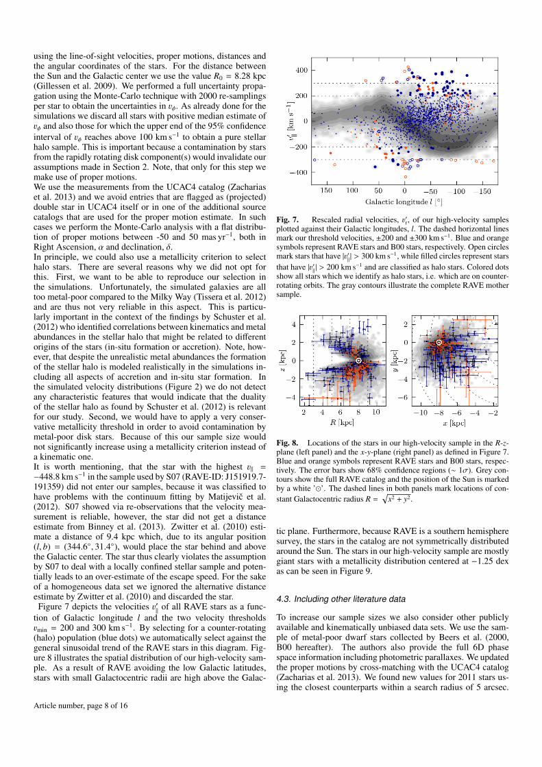
Figure 7 depicts the velocities 3′‖
of all RAVE stars as a func-tion of Galactic longitude l and the two velocity thresholds3min = 200 and 300 km s−1. By selecting for a counter-rotating(halo) population (blue dots) we automatically select against thegeneral sinusoidal trend of the RAVE stars in this diagram. Fig-ure 8 illustrates the spatial distribution of our high-velocity sam-ple. As a result of RAVE avoiding the low Galactic latitudes,stars with small Galactocentric radii are high above the Galac-
Fig. 7. Rescaled radial velocities, 3′r, of our high-velocity samplesplotted against their Galactic longitudes, l. The dashed horizontal linesmark our threshold velocities, ±200 and ±300 km s−1. Blue and orangesymbols represent RAVE stars and B00 stars, respectively. Open circlesmark stars that have |3′
‖| > 300 km s−1, while filled circles represent stars
that have |3′‖| > 200 km s−1 and are classified as halo stars. Colored dots
show all stars which we identify as halo stars, i.e. which are on counter-rotating orbits. The gray contours illustrate the complete RAVE mothersample.
Fig. 8. Locations of the stars in our high-velocity sample in the R-z-plane (left panel) and the x-y-plane (right panel) as defined in Figure 7.Blue and orange symbols represent RAVE stars and B00 stars, respec-tively. The error bars show 68% confidence regions (∼ 1σ). Grey con-tours show the full RAVE catalog and the position of the Sun is markedby a white ’’. The dashed lines in both panels mark locations of con-stant Galactocentric radius R =
√x2 + y2.
tic plane. Furthermore, because RAVE is a southern hemispheresurvey, the stars in the catalog are not symmetrically distributedaround the Sun. The stars in our high-velocity sample are mostlygiant stars with a metallicity distribution centered at −1.25 dexas can be seen in Figure 9.
4.3. Including other literature data
To increase our sample sizes we also consider other publiclyavailable and kinematically unbiased data sets. We use the sam-ple of metal-poor dwarf stars collected by Beers et al. (2000,B00 hereafter). The authors also provide the full 6D phasespace information including photometric parallaxes. We updatedthe proper motions by cross-matching with the UCAC4 catalog(Zacharias et al. 2013). We found new values for 2011 stars us-ing the closest counterparts within a search radius of 5 arcsec.
Article number, page 8 of 16

T. Piffl et al.: The RAVE survey: the Galactic escape speed and the mass of the Milky Way
Fig. 9. Upper panel: Distribution of our high-velocity stars as de-fined in Figure 7 in a Hertzsprung-Russell diagram (symbols with blueerror-bars). For comparison the distribution of all RAVE stars (graycontours) and an isochrone of a stellar population with an age of 10 Gyrand a metallicity of −1 dex (red line) is also shown. The two green sym-bols represent two stars that were excluded from the samples becauseof the their peculiar locations in this diagram. Lower panel: Metallicitydistribution of our high-velocity sample (blue histogram). The blackhistogram shows the metallicity distribution all RAVE stars.
For ten stars we found two sources in the UCAC4 catalog closerthan 5 arcsec and hence discarded these stars. There were further5 cases where two stars in the B00 catalog have the same closestneighbor in the UCAC4 catalog. All these 10 stars were dis-carded as well. Finally, we kept only those stars with uncertain-ties in the line-of-sight velocity measurement below 15 km s−1.There is a small overlap of 123 stars with RAVE, 68 of whichhave got a parallax estimate, $, by Binney et al. (2013) withσ($) < $. By chance two of these stars entered our high-velocity samples. This, on the first glance, very unlikely event isnot so surprising if we consider our selection for halo stars, thestrong bias towards metal-poor halo stars of the B00 catalog andthe significant completeness of the RAVE survey >50% in thebrighter magnitude bins (Kordopatis et al. 2013).In order to compare the two distance estimates we convert alldistances, d, into distance moduli, µ = 5 log(d/10 pc), becauseboth estimates are based on photometry, so the error distributionshould be approximately4 symmetric in this quantity. We findthat σBeers should be about 1.3 mag for the weighted differences(Figure 10, upper panel) to have a standard deviation of unity.B00 quote an uncertainty of 20% on their photometric parallax
4 Note, that Binney et al. (2013) actually showed that the RAVE paral-lax uncertainty distribution is close to normal. However, since both, theRAVE and the B00 distances, are based on the apparent magnitudes ofthe stars, comparing the distance moduli seems to be the better choice,even though the uncertainties are not driven by the uncertainties in thephotometry.
Fig. 10. Upper panel: Distribution of the differences of the distancemodulus estimates, µ, by B00 and Binney et al. (2013), divided by theircombined uncertainty for a RAVE-B00 overlap sample of 68 stars. WithσBeers = 1.3 mag we find a spread of 1σ in the distribution with the me-dian shifted by 0.6σ ' 0.9 mag. The grey curve shows a shifted normaldistribution. The two red data points mark two stars which were alsoentering our high-velocity samples. Lower panel: Direct comparison ofthe two distance estimates with 1 − σ error bars. The solid grey linerepresents equality, while the dashed-dotted line marks equality afterreducing the B00 distances by a factor of 1.5.
estimates, while our estimate corresponds to roughly 60%. Weadopt our more conservative value and emphasize that this uncer-tainty is only used during the selection of counter-rotating halostars.We further find a systematic shift by a factor fdist = 1.5 (δµ = 0.9mag) between the two distance estimates, in the sense that theB00 distances are greater. Since more information was taken intoaccount to derive the RAVE distances we consider them more re-liable. In order to have consistent distances we decrease all B00distances by f −1
dist and use these calibrated values in our furtheranalysis.The data set with the currently most accurately estimated6D phase space coordinates is the Geneva-Copenhagen sur-vey (Nordström et al. 2004) providing Hipparcos distances andproper motions as well as precise radial velocity measurements.However, this survey is confined to a very small volume aroundthe Sun and is therefore even strongly dominated by disk starsthan the RAVE survey. We find only 2 counter-rotating stars inthis sample with |3‖| > 200 km s−1 as well as two (co-rotating)stars with |3‖| > 300 km s−1. For the sake of homogeneity of oursample we neglect these measurements.
Article number, page 9 of 16
5. Results
5.1. Comparison to Smith et al. (2007)
As a first check we do an exact repetition of the analysis appliedby S07 to see whether we get a consistent result. This is inter-esting because strong deviations could point to possible biasesin the data due to, e.g., the slightly increased survey footprintof the sky. RAVE contains 76 stars fulfilling the criteria, whichis an increase by a factor 5 (3 if we take the 19 stars from theB005 catalog into account). The median values of the distribu-tions are effectively the same (537 km s−1 instead of 544 km s−1)and the uncertainties resulting from the 90% confidence inter-val ([504,574]) are reduced by a factor 0.6 (0.7) for the upper(lower) margin, respectively. If we assume that the precision isproportional to the square root of the sample size we expect adecrease in the uncertainties of a factor 3−
12 ' 0.6.
With the distance estimates available now, we know that thisanalysis rests on the incorrect assumption that we deal with alocal sample. If we apply a distance cut dmax = 2.5 kpc ontothe data we obtain a sample of 15 RAVE stars and 16 starsfrom the B00 catalog and we compute a median estimate of526+63
−43 km s−1. A lower value is expected because the distancecriteria removes mainly stars from the inner Galaxy where starsgenerally have higher velocities. The reason for this is thatRAVE is a southern hemisphere survey and therefore observesmostly the inner Galaxy.
5.2. The local escape speed
As described as option (2) in Section 2.1 we can estimate for allstars in the catalogs what their radial velocity would be if theywere situated at the position of the Sun. We then create two sam-ples using the new velocities. For the first sample we select allstars with re-scaled velocities 3′
‖> 300 km s−1. S07 showed that
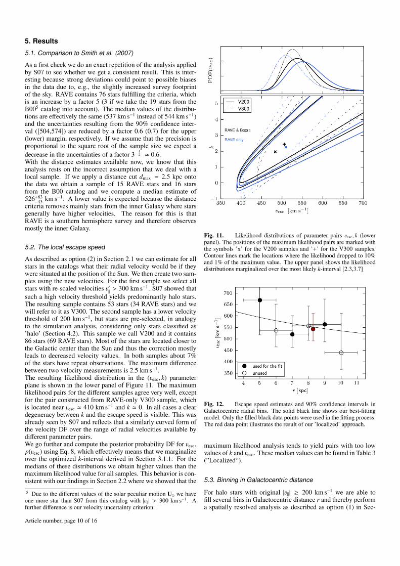
such a high velocity threshold yields predominantly halo stars.The resulting sample contains 53 stars (34 RAVE stars) and wewill refer to it as V300. The second sample has a lower velocitythreshold of 200 km s−1, but stars are pre-selected, in analogyto the simulation analysis, considering only stars classified as’halo’ (Section 4.2). This sample we call V200 and it contains86 stars (69 RAVE stars). Most of the stars are located closer tothe Galactic center than the Sun and thus the correction mostlyleads to decreased velocity values. In both samples about 7%of the stars have repeat observations. The maximum differencebetween two velocity measurements is 2.5 km s−1.The resulting likelihood distribution in the (3esc, k) parameterplane is shown in the lower panel of Figure 11. The maximumlikelihood pairs for the different samples agree very well, exceptfor the pair constructed from RAVE-only V300 sample, whichis located near 3esc ' 410 km s−1 and k ' 0. In all cases a cleardegeneracy between k and the escape speed is visible. This wasalready seen by S07 and reflects that a similarly curved form ofthe velocity DF over the range of radial velocities available bydifferent parameter pairs.We go further and compute the posterior probability DF for 3esc,p(3esc) using Eq. 8, which effectively means that we marginalizeover the optimized k-interval derived in Section 3.1.1. For themedians of these distributions we obtain higher values than themaximum likelihood value for all samples. This behavior is con-sistent with our findings in Section 2.2 where we showed that the
5 Due to the different values of the solar peculiar motion U we haveone more star than S07 from this catalog with |3‖| > 300 km s−1. Afurther difference is our velocity uncertainty criterion.
Fig. 11. Likelihood distributions of parameter pairs 3esc, k (lowerpanel). The positions of the maximum likelihood pairs are marked withthe symbols ’x’ for the V200 samples and ’+’ for the V300 samples.Contour lines mark the locations where the likelihood dropped to 10%and 1% of the maximum value. The upper panel shows the likelihooddistributions marginalized over the most likely k-interval [2.3,3.7]
Fig. 12. Escape speed estimates and 90% confidence intervals inGalactocentric radial bins. The solid black line shows our best-fittingmodel. Only the filled black data points were used in the fitting process.The red data point illustrates the result of our ’localized’ approach.
maximum likelihood analysis tends to yield pairs with too lowvalues of k and 3esc. These median values can be found in Table 3(”Localized“).
5.3. Binning in Galactocentric distance
For halo stars with original |3‖| ≥ 200 km s−1 we are able tofill several bins in Galactocentric distance r and thereby performa spatially resolved analysis as described as option (1) in Sec-
Article number, page 10 of 16
T. Piffl et al.: The RAVE survey: the Galactic escape speed and the mass of the Milky Way
tion 2.1. We chose 6 overlapping bins with a radial width of2 kpc between 4 and 11 kpc. This bin width is larger than theuncertainties of the projected radius estimates for almost all oursample stars (cf. Figure 8). The number of stars in the bins are11, 28, 44, 52, 35 and 8, respectively. The resulting median val-ues (again after marginalizing over the optimal k-interval) of theposterior PDF and the 90% confidence intervals are plotted inFigure 12. The values near the Sun are in very good agreementwith the results of the previous section. We find a rather flat es-cape speed profile except for the out-most bins which containvery few stars, though, and thus have large confidence intervals.
6. Discussion
6.1. Influence of the input parameters
The 90% confidence intervals provided by our analysis tech-nique reflect only the statistical uncertainties resulting from thefinite number of stars in our samples. In this section we considersystematic uncertainties. In Section 3.1.2 we already showedthat our adopted interval for the power-law index k introduces asystematic scatter of about 4%.A further source of uncertainties comes from the motion of theSun relative to the Galactic center. While the radial and ver-tical motion of the Sun is known to very high precision, sev-eral authors have come to different conclusions about the tan-gential motion, V (e.g. Reid & Brunthaler 2004; Bovy et al.2012; Schönrich 2012). In this study we used the standardvalue for VLSR = 220 km s−1 and the V = 12.24 km s−1 fromSchönrich et al. (2010). We repeated the whole analysis usingVLSR = 240 km s−1 and compared the resulting escape speedswith the values of our standard analysis (cf. the lower part of Ta-ble 3). The magnitudes of the deviations are statistically not sig-nificant, but we find systematically lower estimates of the localescape speed for the higher value of VLSR. The shift is close to20 km s−1 and thus comparable to the difference ∆VLSR. This canbe understood if we consider that most stars in the RAVE surveyand – also in our samples – are observed at negative Galacticlongitudes and thus against the direction of Galactic rotation (seeFigure 7). In this case correcting the measured heliocentric line-of-sight velocities with a higher solar tangential motion leads tolower 3‖ which eventually reflects into the escape speed estimate.Note, that this systematic dependency is induced by the half-skynature of the RAVE survey, while for an all-sky survey this ef-fect might cancel out. In contrast, the exact value of R0 is notinfluencing our results, as long as it is kept within the range ofproposed values around 8 kpc.The quantity with the largest uncertainties used in this study isthe heliocentric distance of the stars. In Section 4.3 we founda systematic difference between the distances derived for theRAVE stars and for the stars in the B00 catalog. Such system-atic shifts can arise from various reasons, e.g. different sets oftheoretical isochrones, systematic errors in the stellar parameterestimates or different extinction laws. Again we repeated ouranalysis, this time with all distances increased by a factor 1.5,practically moving to the original distance scale of B00. Againwe find a systematic shift to lower local escape speeds of thesame order as for alternative value of VLSR.We finally also tested the influence of the Galaxy model we useto re-scale the stellar velocities according to their spatial posi-tion. We changed the disk mass to 6.5 × 10¹⁰ M and decreasedthe disk scale radius to 2.5 kpc, in this way preserving the localsurface density of the standard model. The resulting differencesin the corrected velocities are below 1% and no measurable dif-
ference in the escape speed estimates were found illustrating therobustness of our methods to reasonable changes in the Galaxyparameters.
6.2. A critical view on the input assumptions
Our analysis stands and falls with the reliability of our approxi-mation of the velocity DF given in Eq. 1. The conceptual under-pinning of this approximation is very weak for four reasons:
– In many analytic equilibrium models of stellar systems atany spatial point there is a non-zero probability density offinding a star right up to the escape speed 3esc at that point,and zero probability at higher speeds. For example the Jaffe(1983) and Hernquist (1990) models have this property butKing-Michie models (King 1966) do not: in these modelsthe probability density falls to zero at a speed that is smallerthan the escape speed. There is hence an important counter-example to the proposition that n(3) first vanishes at 3 = 3esc.
– All theories of galaxy formation, including the standardΛCDM paradigm, predict that the velocity distribution be-comes radially biased at high speed, so in the context of anequilibrium model there must be significant dependence ofthe DF on the total angular momentum J in addition to E.
– As Spitzer & Thuan (1972) pointed out, in any stellar sys-tem, as E → 0 the periods of orbits diverge. Consequentlythe marginally-bound part of phase space cannot be expectedto be phase mixed. Specifically, stars that are acceleratedto speeds just short of 3esc by fluctuations in Φ in the innersystem take arbitrarily long times to travel to apocenter andreturn to radii where we may hope to study them. Hence dif-ferent mechanisms populate the outgoing and incoming partsof phase space at speeds 3 ∼ 3esc: while parts are populatedby cosmic accretion (Abadi et al. 2009; Teyssier et al. 2009;Piffl et al. 2011), the outgoing part in addition is populatedby slingshot processes (e.g. Hills 1988; Brown et al. 2005)and violent relaxation in the inner galaxy. It follows that wecannot expect the distribution of stars in this portion of phasespace to conform to Jeans theorem, even approximately. YetEq. 1 is founded not just on Jeans theorem but a very specialform of it.
– Counts of stars in the Sloan Digital Sky Survey (SDSS) havemost beautifully demonstrated that the spatial distribution ofhigh-energy stars is very non-smooth. The origin of thesefluctuations in stellar density is widely acknowledged to bethe impact of cosmic accretion, which ensures that at highenergies the DF does not satisfy Jeans theorem.
From this discussion it should be clear that to obtain a cred-ible relationship between the density of fast stars and 3esc wemust engage with the processes that place stars in the marginallybound part of phase space. Fortunately sophisticated simula-tions of galaxy formation in a cosmological context do just that.Figure 2 illustrated that Eq. 1 catches the general shape of thevelocity DF very well. The fact that we find a relatively smallinterval for the power-law index k that fits all simulated galaxieswith their variety of morphologies, argues for the appropriate-ness of the functional form by Leonard & Tremaine (1990).The question remains whether the applied simulation techniqueinfluences the range of k-values we find, since all eight galaxymodels were produced with the same simulation code. In partic-ular, the numerical recipes for so-called sub-grid physics like starformation and stellar energy feedback can have a significant im-pact on the simulation result as was recently demonstrated in the
Article number, page 11 of 16
Aquila code comparison project (Scannapieco et al. 2012). How-ever, the main differences were found in the formation of galaxydisks, while in this study we explicitly focus on the stellar halothat was build up from in-falling satellite galaxies. Differing im-plementations of sub-grid physics might change the amount ofstellar and gas mass being brought in by small galaxies, but itappears unlikely that the phase-space structure of Galactic halowill change significantly. This view is confirmed by the verysimilar k-interval found by S07 using simulations with a com-pletely different implementation of sub-grid physics.
6.3. Estimating the mass of the Milky Way
We now attempt to derive the total mass of the Galaxy usingour escape speed estimates. Doing this we exploit the fact thatthe escape speed is a measure of the local depth of the poten-tial well Φ(R0) = − 1
2 32esc. A critical point in our methodology
is the question whether the velocity distribution reaches up to3esc or whether it is truncated at some lower value. S07 usedtheir simulations to show that the level of truncation in the stel-lar component cannot be more than 10%. However, to test thisthey first had to define the local escape speed by fixing a limitingradius beyond which a star is considered unbound. The authorsstate explicitly that the choice of this radius to be 3Rvir is ratherarbitrary. More stringent would be to state that the velocity dis-tribution in the simulations point to a limiting radius of ∼ 3Rvirbeyond which stars do not fall back onto the galaxy or fall backonly with significantly altered orbital energies, e.g. as part of anin-falling satellite galaxy.It is not a conceptual problem to define the escape speed as thehigh end of the velocity distribution in disregard of the poten-tial profile outside the corresponding limiting radius. Then it isimportant, however, to use the same limiting radius while deriv-ing the total mass of the system using an analytic profile. Thismeans we have to re-define the escape speed to
3esc(r | Rmax) =√
2|Φ(r) − Φ(Rmax)|. (11)
Rmax = 3R340 seems to be an appropriate value (cf. Section 3).This leads to somewhat higher mass estimates. For example, S07found an escape speed of 544 km s−1 and derived a halo mass of0.85 × 1012 M for an NFW profile, practically using Rmax = ∞.If one consistently applies Rmax = 3Rvir the resulting halo massis 1.05 × 10¹² M, an increase by more than 20%. This is thereason why our mass estimates are higher than those by S07 eventhough we find a similar escape speed. Note, that these valuesrepresent the masses of the dark matter halo alone while in theremainder of this study we mean the total mass of the Galaxywhen we refer to the virial mass M340. Keeping this in mind itis then straightforward to compute the virial mass correspondingto a certain local escape speed. As already mentioned, we usethe simple mass model presented in Section 2.In the case of the escape speed profile obtained via the binneddata, the procedure becomes slightly more elaborate. We haveto compute the escape speeds at the centers of the radial binsRi and then take the likelihood from the probability distributionsPDFRi (3esc) in each bin. The product of all these likelihoods6 isthe general likelihood assigned to the mass of the model, i.e.
L(M340) =∏
i
PDFRi (3esc(Ri | M340)) (12)
6 We only use half of the radial bins in order to have statistically inde-pendent measurements.
The results of these mass estimates are presented in Table 3.As already seen in Figure 6 for the simulations the adiabaticallycontracted halo model yields always larger results than the unal-tered halo.
6.4. Fitting the halo concentration parameter
Up to now we assumed a fixed value for the local standard ofrest, VLSR = 220 km s−1, to reduce the number of free parame-ters in our Galaxy model to one. Recently several authors foundlarger values for VLSR of up to 240 km s−1 (e.g. Bovy et al.2012; Schönrich 2012). If we change the parametrization in themodel and use the halo concentration c as a free parameter, wecan compute the likelihood distribution in the (M340, c)-plane inthe same way as described in the previous section. Figure 13plots the resulting likelihood contours for an NFW halo profile(left panel) and the adiabatically contracted NFW profile (rightpanel). The solid black curves mark the locations where the like-lihood dropped to 10% and 1% of the maximum value (whichlies near c ' 0). Grey dotted lines connect locations with com-mon circular velocities at the solar radius.Navarro et al. (1997) showed that the concentration parameter isstrongly related to the mass and the formation time of a dark mat-ter halo (see also Neto et al. 2007; Macciò et al. 2008; Ludlowet al. 2012). With this information we can further constrain therange of likely combinations (M340, c). We use the relation forthe mean concentration as a function of halo mass proposed byMacciò et al. (2008). For this we converted their relation for c200to c340 to be consistent with our definition of the virial radius.There is significant scatter around this relation reflecting the va-riety of formation histories of the halos. This scatter is reason-ably well fitted by a log-normal distribution with σlog c = 0.11(e.g. Macciò et al. 2008; Neto et al. 2007). If we apply this asa prior to our likelihood estimation we obtain the black solidcontours plotted in Figure 13. Note, that in the adiabaticallycontracted case the concentration parameters we are quoting arethe initial concentrations before the contraction. Only these arecomparable to results obtained from dark matter-only simula-tions.The maximum likelihood pair of values (marked by a black ’+’in the figure) for the normal NFW halo is M340 = 1.37×10¹² Mand c = 5, which implies a circular speed of 196 km s−1 at thesolar radius. The adiabatically contracted NFW profile yields thesame c but a somewhat smaller mass of 1.22 × 10¹² M. Herethe resulting circular speed is only 236 km s−1.If we marginalize the likelihood distribution along the c-axis weobtain the one-dimensional posterior PDF for the virial mass.The median and the 90% confidence interval we find to be
M340 = 1.3+0.4−0.3 × 10¹² M
for the un-altered halo profile. For the adiabatically contractedNFW profile we find
M340 = 1.2+0.4−0.3 × 10¹² M ,
in both cases almost identical to the maximum likelihood value.It is worth noting that in this approach the adiabatically con-tracted halo model yields the lower mass estimate, while the op-posite was the case when we fixed the local standard of rest asdone in the previous section.There are several definitions of the virial radius used in the lit-erature. In this study we used the radius which encompassesa mean density of 340 times the critical density for closure inthe universe. If one adopts an over-density of 200 the resulting
Article number, page 12 of 16
T. Piffl et al.: The RAVE survey: the Galactic escape speed and the mass of the Milky Way
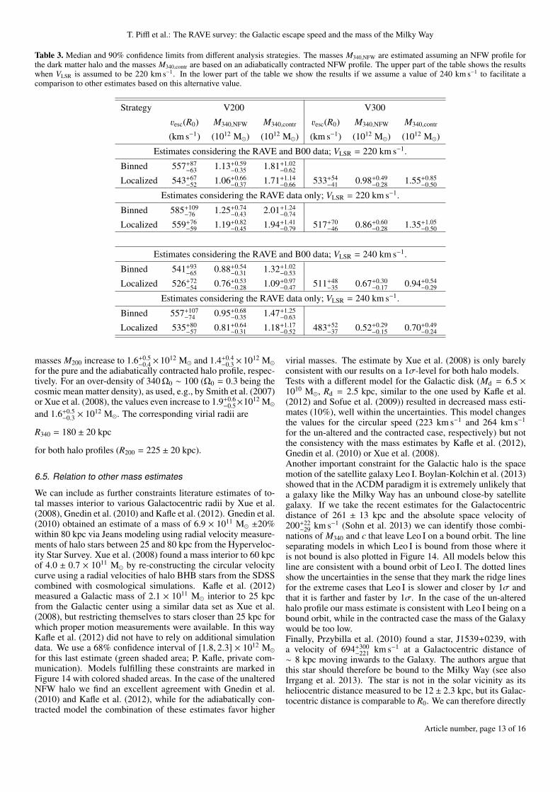
Table 3. Median and 90% confidence limits from different analysis strategies. The masses M340,NFW are estimated assuming an NFW profile forthe dark matter halo and the masses M340,contr are based on an adiabatically contracted NFW profile. The upper part of the table shows the resultswhen VLSR is assumed to be 220 km s−1. In the lower part of the table we show the results if we assume a value of 240 km s−1 to facilitate acomparison to other estimates based on this alternative value.
Strategy V200 V300
3esc(R0) M340,NFW M340,contr 3esc(R0) M340,NFW M340,contr
(km s−1) (1012 M) (1012 M) (km s−1) (1012 M) (1012 M)
Estimates considering the RAVE and B00 data; VLSR = 220 km s−1.
Binned 557+87−63 1.13+0.59
−0.35 1.81+1.02−0.62
Localized 543+67−52 1.06+0.66
−0.37 1.71+1.14−0.66 533+54
−41 0.98+0.49−0.28 1.55+0.85
−0.50
Estimates considering the RAVE data only; VLSR = 220 km s−1.
Binned 585+109−76 1.25+0.74
−0.43 2.01+1.24−0.74
Localized 559+76−59 1.19+0.82
−0.45 1.94+1.41−0.79 517+70
−46 0.86+0.60−0.28 1.35+1.05
−0.50
Estimates considering the RAVE and B00 data; VLSR = 240 km s−1.
Binned 541+93−65 0.88+0.54
−0.31 1.32+1.02−0.53
Localized 526+72−54 0.76+0.53
−0.28 1.09+0.97−0.47 511+48
−35 0.67+0.30−0.17 0.94+0.54
−0.29
Estimates considering the RAVE data only; VLSR = 240 km s−1.
Binned 557+107−74 0.95+0.68
−0.35 1.47+1.25−0.63
Localized 535+80−57 0.81+0.64
−0.31 1.18+1.17−0.52 483+52
−37 0.52+0.29−0.15 0.70+0.49
−0.24
masses M200 increase to 1.6+0.5−0.4 × 10¹² M and 1.4+0.4
−0.3 × 10¹² Mfor the pure and the adiabatically contracted halo profile, respec-tively. For an over-density of 340 Ω0 ∼ 100 (Ω0 = 0.3 being thecosmic mean matter density), as used, e.g., by Smith et al. (2007)or Xue et al. (2008), the values even increase to 1.9+0.6
−0.5×10¹² Mand 1.6+0.5
−0.3 × 10¹² M. The corresponding virial radii are
R340 = 180 ± 20 kpc
for both halo profiles (R200 = 225 ± 20 kpc).
6.5. Relation to other mass estimates
We can include as further constraints literature estimates of to-tal masses interior to various Galactocentric radii by Xue et al.(2008), Gnedin et al. (2010) and Kafle et al. (2012). Gnedin et al.(2010) obtained an estimate of a mass of 6.9 × 10¹¹ M ±20%within 80 kpc via Jeans modeling using radial velocity measure-ments of halo stars between 25 and 80 kpc from the Hyperveloc-ity Star Survey. Xue et al. (2008) found a mass interior to 60 kpcof 4.0 ± 0.7 × 10¹¹ M by re-constructing the circular velocitycurve using a radial velocities of halo BHB stars from the SDSScombined with cosmological simulations. Kafle et al. (2012)measured a Galactic mass of 2.1 × 10¹¹ M interior to 25 kpcfrom the Galactic center using a similar data set as Xue et al.(2008), but restricting themselves to stars closer than 25 kpc forwhich proper motion measurements were available. In this wayKafle et al. (2012) did not have to rely on additional simulationdata. We use a 68% confidence interval of [1.8, 2.3] × 1012 Mfor this last estimate (green shaded area; P. Kafle, private com-munication). Models fulfilling these constraints are marked inFigure 14 with colored shaded areas. In the case of the unalteredNFW halo we find an excellent agreement with Gnedin et al.(2010) and Kafle et al. (2012), while for the adiabatically con-tracted model the combination of these estimates favor higher
virial masses. The estimate by Xue et al. (2008) is only barelyconsistent with our results on a 1σ-level for both halo models.Tests with a different model for the Galactic disk (Md = 6.5 ×10¹⁰ M, Rd = 2.5 kpc, similar to the one used by Kafle et al.(2012) and Sofue et al. (2009)) resulted in decreased mass esti-mates (10%), well within the uncertainties. This model changesthe values for the circular speed (223 km s−1 and 264 km s−1
for the un-altered and the contracted case, respectively) but notthe consistency with the mass estimates by Kafle et al. (2012),Gnedin et al. (2010) or Xue et al. (2008).Another important constraint for the Galactic halo is the spacemotion of the satellite galaxy Leo I. Boylan-Kolchin et al. (2013)showed that in the ΛCDM paradigm it is extremely unlikely thata galaxy like the Milky Way has an unbound close-by satellitegalaxy. If we take the recent estimates for the Galactocentricdistance of 261 ± 13 kpc and the absolute space velocity of200+22
−29 km s−1 (Sohn et al. 2013) we can identify those combi-nations of M340 and c that leave Leo I on a bound orbit. The lineseparating models in which Leo I is bound from those where itis not bound is also plotted in Figure 14. All models below thisline are consistent with a bound orbit of Leo I. The dotted linesshow the uncertainties in the sense that they mark the ridge linesfor the extreme cases that Leo I is slower and closer by 1σ andthat it is farther and faster by 1σ. In the case of the un-alteredhalo profile our mass estimate is consistent with Leo I being on abound orbit, while in the contracted case the mass of the Galaxywould be too low.Finally, Przybilla et al. (2010) found a star, J1539+0239, witha velocity of 694+300
−221 km s−1 at a Galactocentric distance of∼ 8 kpc moving inwards to the Galaxy. The authors argue thatthis star should therefore be bound to the Milky Way (see alsoIrrgang et al. 2013). The star is not in the solar vicinity as itsheliocentric distance measured to be 12 ± 2.3 kpc, but its Galac-tocentric distance is comparable to R0. We can therefore directly
Article number, page 13 of 16
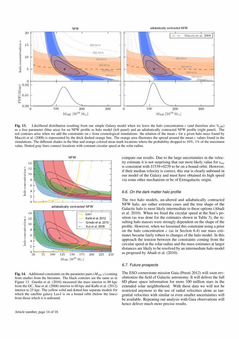
Fig. 13. Likelihood distribution resulting from our simple Galaxy model when we leave the halo concentration c (and therefore also VLSR)as a free parameter (blue area) for an NFW profile as halo model (left panel) and an adiabatically contracted NFW profile (right panel). Thered contours arise when we add the constraints on c from cosmological simulations: the relation of the mean c for a given halo mass found byMacciò et al. (2008) is represented by the thick dashed orange line. The orange area illustrates the spread around the mean c values found in thesimulations. The different shades in the blue and orange colored areas mark locations where the probability dropped to 10%, 1% of the maximumvalue. Dotted gray lines connect locations with constant circular speed at the solar radius.
Fig. 14. Additional constraints on the parameter pairs (M340, c) comingfrom studies from the literature. The black contours are the same as inFigure 13. Gnedin et al. (2010) measured the mass interior to 80 kpcfrom the GC, Xue et al. (2008) interior to 60 kpc and Kafle et al. (2012)interior to 25 kpc. The yellow solid and dotted line separate models forwhich the satellite galaxy Leo I is on a bound orbit (below the lines)from those which it is unbound.
compare our results. Due to the large uncertainties in the veloc-ity estimate it is not surprising that our most likely value for 3escis consistent with J1539+0239 to be on a bound orbit. However,if their median velocity is correct, this star is clearly unbound inour model of the Galaxy and must have obtained its high speedvia some other mechanism or be of Extragalactic origin.
6.6. On the dark matter halo profile
The two halo models, un-altered and adiabatically contractedNFW halo, are rather extreme cases and the true shape of theGalactic halo is most likely intermediate to these options (Abadiet al. 2010). When we fixed the circular speed at the Sun’s po-sition (as was done for the estimates shown in Table 3), the re-sulting halo masses were strongly dependent on the shape of theprofile. However, when we loosened this constraint using a prioron the halo concentration c (as in Section 6.4) our mass esti-mates became fairly robust to changes of the halo model. In thisapproach the tension between the constraints coming from thecircular speed at the solar radius and the mass estimates at largerdistances are likely to be resolved by an intermediate halo modelas proposed by Abadi et al. (2010).
6.7. Future prospects
The ESO cornerstone mission Gaia (Prusti 2012) will soon rev-olutionize the field of Galactic astronomy. It will deliver the full6D phase space information for more 100 million stars in theextended solar neighborhood. With these data we will not berestricted anymore to the use of radial velocities alone as tan-gential velocities with similar or even smaller uncertainties willbe available. Repeating our analysis with Gaia observations willhence deliver much more precise results.
Article number, page 14 of 16
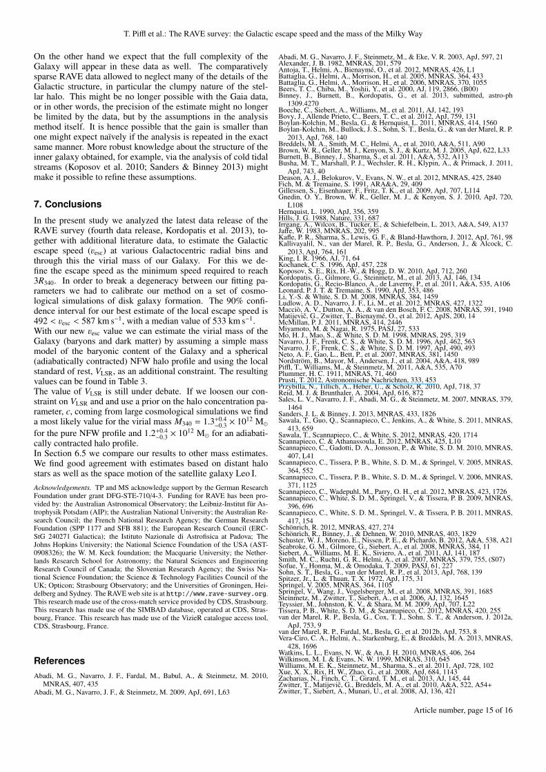
T. Piffl et al.: The RAVE survey: the Galactic escape speed and the mass of the Milky Way
On the other hand we expect that the full complexity of theGalaxy will appear in these data as well. The comparativelysparse RAVE data allowed to neglect many of the details of theGalactic structure, in particular the clumpy nature of the stel-lar halo. This might be no longer possible with the Gaia data,or in other words, the precision of the estimate might no longerbe limited by the data, but by the assumptions in the analysismethod itself. It is hence possible that the gain is smaller thanone might expect naïvely if the analysis is repeated in the exactsame manner. More robust knowledge about the structure of theinner galaxy obtained, for example, via the analysis of cold tidalstreams (Koposov et al. 2010; Sanders & Binney 2013) mightmake it possible to refine these assumptions.
7. Conclusions
In the present study we analyzed the latest data release of theRAVE survey (fourth data release, Kordopatis et al. 2013), to-gether with additional literature data, to estimate the Galacticescape speed (3esc) at various Galactocentric radial bins andthrough this the virial mass of our Galaxy. For this we de-fine the escape speed as the minimum speed required to reach3R340. In order to break a degeneracy between our fitting pa-rameters we had to calibrate our method on a set of cosmo-logical simulations of disk galaxy formation. The 90% confi-dence interval for our best estimate of the local escape speed is492 < 3esc < 587 km s−1, with a median value of 533 km s−1.With our new 3esc value we can estimate the virial mass of theGalaxy (baryons and dark matter) by assuming a simple massmodel of the baryonic content of the Galaxy and a spherical(adiabatically contracted) NFW halo profile and using the localstandard of rest, VLSR, as an additional constraint. The resultingvalues can be found in Table 3.The value of VLSR is still under debate. If we loosen our con-straint on VLSR and and use a prior on the halo concentration pa-rameter, c, coming from large cosmological simulations we finda most likely value for the virial mass M340 = 1.3+0.4
−0.3 × 10¹² Mfor the pure NFW profile and 1.2+0.4
−0.3 × 10¹² M for an adiabati-cally contracted halo profile.In Section 6.5 we compare our results to other mass estimates.We find good agreement with estimates based on distant halostars as well as the space motion of the satellite galaxy Leo I.Acknowledgements. TP and MS acknowledge support by the German ResearchFoundation under grant DFG-STE-710/4-3. Funding for RAVE has been pro-vided by: the Australian Astronomical Observatory; the Leibniz-Institut für As-trophysik Potsdam (AIP); the Australian National University; the Australian Re-search Council; the French National Research Agency; the German ResearchFoundation (SPP 1177 and SFB 881); the European Research Council (ERC-StG 240271 Galactica); the Istituto Nazionale di Astrofisica at Padova; TheJohns Hopkins University; the National Science Foundation of the USA (AST-0908326); the W. M. Keck foundation; the Macquarie University; the Nether-lands Research School for Astronomy; the Natural Sciences and EngineeringResearch Council of Canada; the Slovenian Research Agency; the Swiss Na-tional Science Foundation; the Science & Technology Facilities Council of theUK; Opticon; Strasbourg Observatory; and the Universities of Groningen, Hei-delberg and Sydney. The RAVE web site is at http://www.rave-survey.org.This research made use of the cross-match service provided by CDS, Strasbourg.This research has made use of the SIMBAD database, operated at CDS, Stras-bourg, France. This research has made use of the VizieR catalogue access tool,CDS, Strasbourg, France.
ReferencesAbadi, M. G., Navarro, J. F., Fardal, M., Babul, A., & Steinmetz, M. 2010,
MNRAS, 407, 435Abadi, M. G., Navarro, J. F., & Steinmetz, M. 2009, ApJ, 691, L63
Abadi, M. G., Navarro, J. F., Steinmetz, M., & Eke, V. R. 2003, ApJ, 597, 21Alexander, J. B. 1982, MNRAS, 201, 579Antoja, T., Helmi, A., Bienaymé, O., et al. 2012, MNRAS, 426, L1Battaglia, G., Helmi, A., Morrison, H., et al. 2005, MNRAS, 364, 433Battaglia, G., Helmi, A., Morrison, H., et al. 2006, MNRAS, 370, 1055Beers, T. C., Chiba, M., Yoshii, Y., et al. 2000, AJ, 119, 2866, (B00)Binney, J., Burnett, B., Kordopatis, G., et al. 2013, submitted, astro-ph
1309.4270Boeche, C., Siebert, A., Williams, M., et al. 2011, AJ, 142, 193Bovy, J., Allende Prieto, C., Beers, T. C., et al. 2012, ApJ, 759, 131Boylan-Kolchin, M., Besla, G., & Hernquist, L. 2011, MNRAS, 414, 1560Boylan-Kolchin, M., Bullock, J. S., Sohn, S. T., Besla, G., & van der Marel, R. P.
2013, ApJ, 768, 140Breddels, M. A., Smith, M. C., Helmi, A., et al. 2010, A&A, 511, A90Brown, W. R., Geller, M. J., Kenyon, S. J., & Kurtz, M. J. 2005, ApJ, 622, L33Burnett, B., Binney, J., Sharma, S., et al. 2011, A&A, 532, A113Busha, M. T., Marshall, P. J., Wechsler, R. H., Klypin, A., & Primack, J. 2011,
ApJ, 743, 40Deason, A. J., Belokurov, V., Evans, N. W., et al. 2012, MNRAS, 425, 2840Fich, M. & Tremaine, S. 1991, ARA&A, 29, 409Gillessen, S., Eisenhauer, F., Fritz, T. K., et al. 2009, ApJ, 707, L114Gnedin, O. Y., Brown, W. R., Geller, M. J., & Kenyon, S. J. 2010, ApJ, 720,
L108Hernquist, L. 1990, ApJ, 356, 359Hills, J. G. 1988, Nature, 331, 687Irrgang, A., Wilcox, B., Tucker, E., & Schiefelbein, L. 2013, A&A, 549, A137Jaffe, W. 1983, MNRAS, 202, 995Kafle, P. R., Sharma, S., Lewis, G. F., & Bland-Hawthorn, J. 2012, ApJ, 761, 98Kallivayalil, N., van der Marel, R. P., Besla, G., Anderson, J., & Alcock, C.
2013, ApJ, 764, 161King, I. R. 1966, AJ, 71, 64Kochanek, C. S. 1996, ApJ, 457, 228Koposov, S. E., Rix, H.-W., & Hogg, D. W. 2010, ApJ, 712, 260Kordopatis, G., Gilmore, G., Steinmetz, M., et al. 2013, AJ, 146, 134Kordopatis, G., Recio-Blanco, A., de Laverny, P., et al. 2011, A&A, 535, A106Leonard, P. J. T. & Tremaine, S. 1990, ApJ, 353, 486Li, Y.-S. & White, S. D. M. 2008, MNRAS, 384, 1459Ludlow, A. D., Navarro, J. F., Li, M., et al. 2012, MNRAS, 427, 1322Macciò, A. V., Dutton, A. A., & van den Bosch, F. C. 2008, MNRAS, 391, 1940Matijevic, G., Zwitter, T., Bienaymé, O., et al. 2012, ApJS, 200, 14McMillan, P. J. 2011, MNRAS, 414, 2446Miyamoto, M. & Nagai, R. 1975, PASJ, 27, 533Mo, H. J., Mao, S., & White, S. D. M. 1998, MNRAS, 295, 319Navarro, J. F., Frenk, C. S., & White, S. D. M. 1996, ApJ, 462, 563Navarro, J. F., Frenk, C. S., & White, S. D. M. 1997, ApJ, 490, 493Neto, A. F., Gao, L., Bett, P., et al. 2007, MNRAS, 381, 1450Nordström, B., Mayor, M., Andersen, J., et al. 2004, A&A, 418, 989Piffl, T., Williams, M., & Steinmetz, M. 2011, A&A, 535, A70Plummer, H. C. 1911, MNRAS, 71, 460Prusti, T. 2012, Astronomische Nachrichten, 333, 453Przybilla, N., Tillich, A., Heber, U., & Scholz, R. 2010, ApJ, 718, 37Reid, M. J. & Brunthaler, A. 2004, ApJ, 616, 872Sales, L. V., Navarro, J. F., Abadi, M. G., & Steinmetz, M. 2007, MNRAS, 379,
1464Sanders, J. L. & Binney, J. 2013, MNRAS, 433, 1826Sawala, T., Guo, Q., Scannapieco, C., Jenkins, A., & White, S. 2011, MNRAS,
413, 659Sawala, T., Scannapieco, C., & White, S. 2012, MNRAS, 420, 1714Scannapieco, C. & Athanassoula, E. 2012, MNRAS, 425, L10Scannapieco, C., Gadotti, D. A., Jonsson, P., & White, S. D. M. 2010, MNRAS,
407, L41Scannapieco, C., Tissera, P. B., White, S. D. M., & Springel, V. 2005, MNRAS,
364, 552Scannapieco, C., Tissera, P. B., White, S. D. M., & Springel, V. 2006, MNRAS,
371, 1125Scannapieco, C., Wadepuhl, M., Parry, O. H., et al. 2012, MNRAS, 423, 1726Scannapieco, C., White, S. D. M., Springel, V., & Tissera, P. B. 2009, MNRAS,
396, 696Scannapieco, C., White, S. D. M., Springel, V., & Tissera, P. B. 2011, MNRAS,
417, 154Schönrich, R. 2012, MNRAS, 427, 274Schönrich, R., Binney, J., & Dehnen, W. 2010, MNRAS, 403, 1829Schuster, W. J., Moreno, E., Nissen, P. E., & Pichardo, B. 2012, A&A, 538, A21Seabroke, G. M., Gilmore, G., Siebert, A., et al. 2008, MNRAS, 384, 11Siebert, A., Williams, M. E. K., Siviero, A., et al. 2011, AJ, 141, 187Smith, M. C., Ruchti, G. R., Helmi, A., et al. 2007, MNRAS, 379, 755, (S07)Sofue, Y., Honma, M., & Omodaka, T. 2009, PASJ, 61, 227Sohn, S. T., Besla, G., van der Marel, R. P., et al. 2013, ApJ, 768, 139Spitzer, Jr., L. & Thuan, T. X. 1972, ApJ, 175, 31Springel, V. 2005, MNRAS, 364, 1105Springel, V., Wang, J., Vogelsberger, M., et al. 2008, MNRAS, 391, 1685Steinmetz, M., Zwitter, T., Siebert, A., et al. 2006, AJ, 132, 1645Teyssier, M., Johnston, K. V., & Shara, M. M. 2009, ApJ, 707, L22Tissera, P. B., White, S. D. M., & Scannapieco, C. 2012, MNRAS, 420, 255van der Marel, R. P., Besla, G., Cox, T. J., Sohn, S. T., & Anderson, J. 2012a,
ApJ, 753, 9van der Marel, R. P., Fardal, M., Besla, G., et al. 2012b, ApJ, 753, 8Vera-Ciro, C. A., Helmi, A., Starkenburg, E., & Breddels, M. A. 2013, MNRAS,
428, 1696Watkins, L. L., Evans, N. W., & An, J. H. 2010, MNRAS, 406, 264Wilkinson, M. I. & Evans, N. W. 1999, MNRAS, 310, 645Williams, M. E. K., Steinmetz, M., Sharma, S., et al. 2011, ApJ, 728, 102Xue, X. X., Rix, H. W., Zhao, G., et al. 2008, ApJ, 684, 1143Zacharias, N., Finch, C. T., Girard, T. M., et al. 2013, AJ, 145, 44Zwitter, T., Matijevic, G., Breddels, M. A., et al. 2010, A&A, 522, A54+Zwitter, T., Siebert, A., Munari, U., et al. 2008, AJ, 136, 421
Article number, page 15 of 16
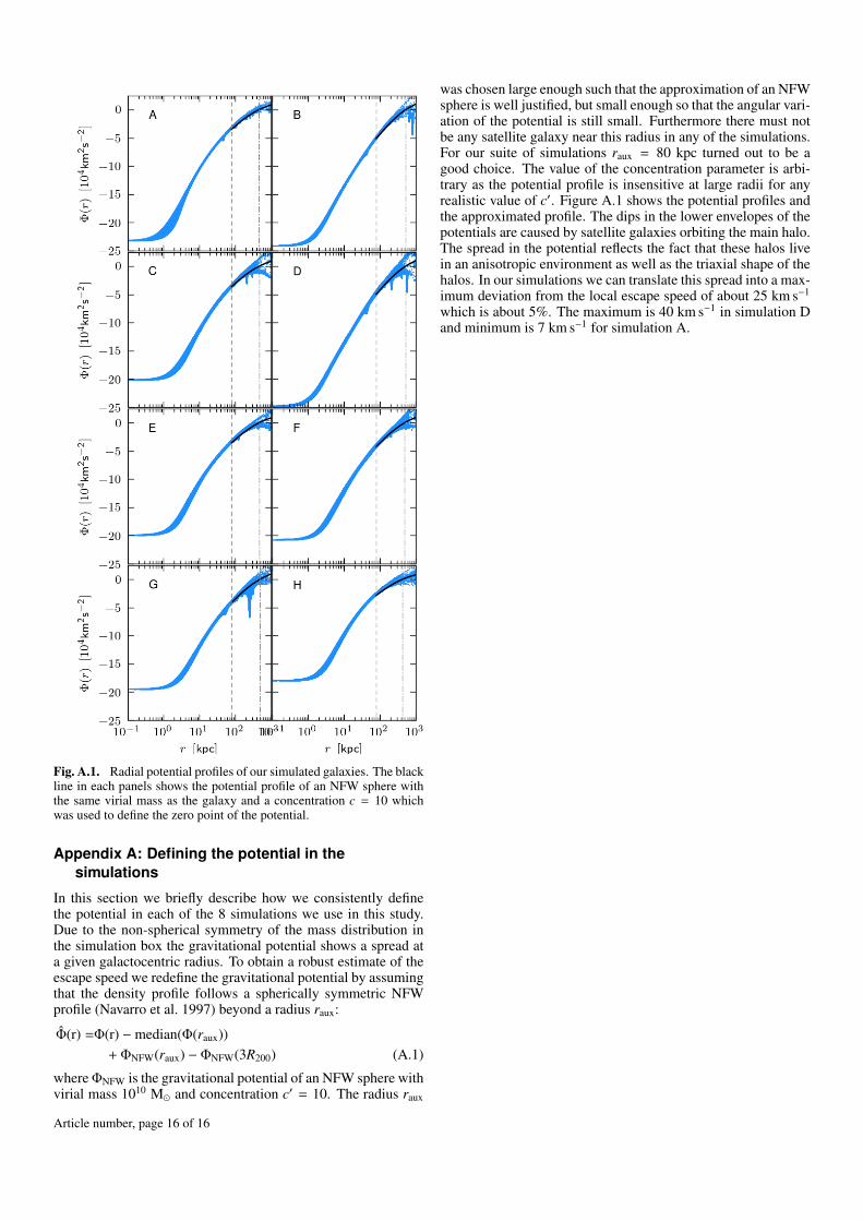
Fig. A.1. Radial potential profiles of our simulated galaxies. The blackline in each panels shows the potential profile of an NFW sphere withthe same virial mass as the galaxy and a concentration c = 10 whichwas used to define the zero point of the potential.
Appendix A: Defining the potential in thesimulations
In this section we briefly describe how we consistently definethe potential in each of the 8 simulations we use in this study.Due to the non-spherical symmetry of the mass distribution inthe simulation box the gravitational potential shows a spread ata given galactocentric radius. To obtain a robust estimate of theescape speed we redefine the gravitational potential by assumingthat the density profile follows a spherically symmetric NFWprofile (Navarro et al. 1997) beyond a radius raux:
Φ(r) =Φ(r) −median(Φ(raux))+ ΦNFW(raux) − ΦNFW(3R200) (A.1)
where ΦNFW is the gravitational potential of an NFW sphere withvirial mass 1010 M and concentration c′ = 10. The radius raux
was chosen large enough such that the approximation of an NFWsphere is well justified, but small enough so that the angular vari-ation of the potential is still small. Furthermore there must notbe any satellite galaxy near this radius in any of the simulations.For our suite of simulations raux = 80 kpc turned out to be agood choice. The value of the concentration parameter is arbi-trary as the potential profile is insensitive at large radii for anyrealistic value of c′. Figure A.1 shows the potential profiles andthe approximated profile. The dips in the lower envelopes of thepotentials are caused by satellite galaxies orbiting the main halo.The spread in the potential reflects the fact that these halos livein an anisotropic environment as well as the triaxial shape of thehalos. In our simulations we can translate this spread into a max-imum deviation from the local escape speed of about 25 km s−1
which is about 5%. The maximum is 40 km s−1 in simulation Dand minimum is 7 km s−1 for simulation A.
Article number, page 16 of 16
Related Documents