THE QUARTERLY JOURNAL OF ECONOMICS Vol. 133 May 2018 Issue 2 DISTRIBUTIONAL NATIONAL ACCOUNTS: METHODS AND ESTIMATES FOR THE UNITED STATES ∗ THOMAS PIKETTY EMMANUEL SAEZ GABRIEL ZUCMAN This article combines tax, survey, and national accounts data to estimate the distribution of national income in the United States since 1913. Our distributional national accounts capture 100% of national income, allowing us to compute growth rates for each quantile of the income distribution consistent with macroeconomic growth. We estimate the distribution of both pretax and posttax income, making it possible to provide a comprehensive view of how government redistribution affects inequality. Average pretax real national income per adult has increased 60% from 1980 to 2014, but we find that it has stagnated for the bottom 50% of the distribution at about $16,000 a year. The pretax income of the middle class—adults between the median and the 90th percentile—has grown 40% since 1980, faster than what tax and survey data suggest, due in particular to the rise of tax-exempt fringe benefits. Income has boomed at the top. The upsurge of top incomes was first a labor income phenomenon but has mostly been a capital income phenomenon ∗ We thank the editors, Lawrence Katz and Andrei Shleifer; four anony- mous referees; Facundo Alvaredo, Tony Atkinson, Gerald Auten, Lucas Chancel, Patrick Driessen, Oded Galor, David Johnson, Arthur Kennickell, Nora Lustig, Jean-Laurent Rosenthal, John Sabelhaus, David Splinter, and Danny Yagan; and numerous seminar and conference participants for helpful discussions and com- ments. Antoine Arnoud, Kaveh Danesh, Sam Karlin, Juliana Londo ˜ no-V´ elez, and Carl McPherson provided outstanding research assistance. We acknowledge finan- cial support from the Center for Equitable Growth at UC Berkeley, the Institute for New Economic Thinking, the Laura and John Arnold foundation, NSF grants SES-1156240 and SES-1559014, the Russell Sage foundation, the Sandler foun- dation, and the European Research Council under the European Union’s Seventh Framework Programme, ERC Grant Agreement No. 340831. C The Author(s) 2017. Published by Oxford University Press on behalf of the Presi- dent and Fellows of Harvard College. All rights reserved. For Permissions, please email: [email protected] The Quarterly Journal of Economics (2018), 553–609. doi:10.1093/qje/qjx043. Advance Access publication on October 10, 2017. 553 Downloaded from https://academic.oup.com/qje/article-abstract/133/2/553/4430651 by guest on 01 April 2018

Welcome message from author
This document is posted to help you gain knowledge. Please leave a comment to let me know what you think about it! Share it to your friends and learn new things together.
Transcript

THE
QUARTERLY JOURNALOF ECONOMICS
Vol. 133 May 2018 Issue 2
DISTRIBUTIONAL NATIONAL ACCOUNTS: METHODS ANDESTIMATES FOR THE UNITED STATES∗
THOMAS PIKETTY
EMMANUEL SAEZ
GABRIEL ZUCMAN
This article combines tax, survey, and national accounts data to estimate thedistribution of national income in the United States since 1913. Our distributionalnational accounts capture 100% of national income, allowing us to compute growthrates for each quantile of the income distribution consistent with macroeconomicgrowth. We estimate the distribution of both pretax and posttax income, makingit possible to provide a comprehensive view of how government redistributionaffects inequality. Average pretax real national income per adult has increased60% from 1980 to 2014, but we find that it has stagnated for the bottom 50% of thedistribution at about $16,000 a year. The pretax income of the middle class—adultsbetween the median and the 90th percentile—has grown 40% since 1980, fasterthan what tax and survey data suggest, due in particular to the rise of tax-exemptfringe benefits. Income has boomed at the top. The upsurge of top incomes was firsta labor income phenomenon but has mostly been a capital income phenomenon
∗We thank the editors, Lawrence Katz and Andrei Shleifer; four anony-mous referees; Facundo Alvaredo, Tony Atkinson, Gerald Auten, Lucas Chancel,Patrick Driessen, Oded Galor, David Johnson, Arthur Kennickell, Nora Lustig,Jean-Laurent Rosenthal, John Sabelhaus, David Splinter, and Danny Yagan; andnumerous seminar and conference participants for helpful discussions and com-ments. Antoine Arnoud, Kaveh Danesh, Sam Karlin, Juliana Londono-Velez, andCarl McPherson provided outstanding research assistance. We acknowledge finan-cial support from the Center for Equitable Growth at UC Berkeley, the Institutefor New Economic Thinking, the Laura and John Arnold foundation, NSF grantsSES-1156240 and SES-1559014, the Russell Sage foundation, the Sandler foun-dation, and the European Research Council under the European Union’s SeventhFramework Programme, ERC Grant Agreement No. 340831.
C© The Author(s) 2017. Published by Oxford University Press on behalf of the Presi-dent and Fellows of Harvard College. All rights reserved. For Permissions, please email:[email protected] Quarterly Journal of Economics (2018), 553–609. doi:10.1093/qje/qjx043.Advance Access publication on October 10, 2017.
553Downloaded from https://academic.oup.com/qje/article-abstract/133/2/553/4430651by gueston 01 April 2018
554 QUARTERLY JOURNAL OF ECONOMICS
since 2000. The government has offset only a small fraction of the increase ininequality. The reduction of the gender gap in earnings has mitigated the increasein inequality among adults, but the share of women falls steeply as one moves upthe labor income distribution, and is only 11% in the top 0.1% in 2014. JEL Codes:E01, H2, H5, J3.
I. INTRODUCTION
Income inequality has increased in many developed coun-tries over the past several decades. This trend has attractedconsiderable interest among academics, policy makers, and thegeneral public. In recent years, following up on Kuznets’ (1953)pioneering attempt, a number of authors have used administra-tive tax records to construct long-run series of top income shares(Alvaredo et al. 2011–2017). Despite this endeavor, we still facethree important limitations when measuring income inequality.First and most important, there is a large gap between nationalaccounts—which focus on macro totals and growth—and inequal-ity studies—which focus on distributions using survey and taxdata, usually without trying to be fully consistent with macro to-tals. This gap makes it hard to address questions such as: whatfraction of economic growth accrues to the bottom 50%, the middle40%, and the top 10% of the distribution? How much of the rise inincome inequality owes to changes in the share of labor and capi-tal in national income, and how much to changes in the dispersionof labor earnings, capital ownership, and returns to capital? Sec-ond, about a third of U.S. national income is redistributed throughtaxes, transfers, and public spending on goods and services suchas education, police, and defense. Yet we do not have a compre-hensive measure of how the distribution of pretax income differsfrom the distribution of posttax income, making it hard to assesshow government redistribution affects inequality. Third, existingincome inequality statistics use the tax unit or the household asunit of observation, adding up the income of men and women. Asa result, we do not have a clear view of how long-run trends in in-come concentration are shaped by the major changes in women’slabor force participation—and gender inequality generally—thathave occurred over the past century.
This article attempts to compute inequality statistics for theUnited States that overcome the limits of existing series by cre-ating distributional national accounts. We combine tax, survey,and national accounts data to build new series on the distributionof national income since 1913. In contrast to previous attempts
Downloaded from https://academic.oup.com/qje/article-abstract/133/2/553/4430651by gueston 01 April 2018

DISTRIBUTIONAL NATIONAL ACCOUNTS 555
that capture less than 60% of U.S. national income—such as Cen-sus Bureau estimates (U.S. Census Bureau 2016) and top incomeshares (Piketty and Saez 2003)—our estimates capture 100% ofthe national income recorded in the national accounts. This en-ables us to provide decompositions of growth by income groupsconsistent with macroeconomic growth. We compute the distri-bution of both pretax and posttax income. Posttax series deductall taxes and add back all transfers and public spending, so thatboth pretax and posttax incomes add up to national income. Thisallows us to provide the first comprehensive view of how govern-ment redistribution affects inequality. Our benchmark series usesthe adult individual as the unit of observation and splits incomeequally among spouses. We also report series in which each spouseis assigned her or his own labor income, enabling us to study howlong-run changes in gender inequality shape the distribution ofincome.
Distributional national accounts provide information on thedynamics of income across the entire spectrum—from the bot-tom decile to the top 0.001%—which, we believe, is more accuratethan existing inequality data. Our estimates capture employeefringe benefits, a growing source of income for the middle classoverlooked by both Census Bureau estimates and tax data. Theycapture all capital income, which is large (about 30% of total na-tional income) and concentrated, yet is very imperfectly coveredby surveys (due to small sample and top-coding issues) and by taxdata, as a large fraction of capital income goes to pension fundsand is retained in corporations. They make it possible to producelong-run inequality statistics that control for socio-demographicchanges—such as the rise in the fraction of retired individuals andthe decline in household size—contrary to the currently availabletax-based series.
Methodologically, our contribution is to construct micro-filesof pretax and posttax income consistent with macro aggregates.These micro-files contain all the variables of the national accountsand synthetic adult individual observations that we obtain by sta-tistically matching tax and survey data and making explicit as-sumptions about the distribution of income categories for whichthere is no directly available source of information. By construc-tion, the totals in these micro-files add up to the national accountstotals, while the distributions are consistent with those seen in taxand survey data. These files can be used to compute a wide array ofdistributional statistics—labor and capital income earned, taxespaid, transfers received, wealth owned, and so on—by age groups,
Downloaded from https://academic.oup.com/qje/article-abstract/133/2/553/4430651by gueston 01 April 2018

556 QUARTERLY JOURNAL OF ECONOMICS
gender, and marital status. Our objective, in the years ahead, isto construct similar micro-files in as many countries as possible tobetter compare inequality across countries.1 Just like we use GDPor national income to compare the macroeconomic performancesof countries today, so could distributional national accounts beused to compare inequality across countries tomorrow.
We stress at the outset that there are numerous data issuesinvolved in distributing national income, discussed in the textand the Online Appendix.2 First, we take the national accountsas a given starting point, although we are well aware that thenational accounts themselves are imperfect (e.g., Zucman 2013).They are, however, the most reasonable starting point, becausethey aggregate all the available information from surveys, taxdata, corporate income statements and balance sheets, and so on,in a standardized, internationally agreed on, and regularly im-proved accounting framework. Second, imputing all national in-come, taxes, transfers, and public goods spending requires makingassumptions on a number of complex issues, such as the economicincidence of taxes and who benefits from government spending.Our goal is not to provide definitive answers to these questionsbut to be comprehensive, consistent, and explicit about what as-sumptions we are making and why. We view our article as at-tempting to construct prototype distributional national accounts,a prototype that could be improved upon as more data becomeavailable, new knowledge emerges on who pays taxes and whobenefits from government spending, and refined estimation tech-niques are developed—just as today’s national accounts are regu-larly improved. Third, our estimates of incomes at the top of thedistribution are based on tax data, and hence disregard tax eva-sion. Because top marginal tax rates, tax evasion technologies,and tax enforcement strategies have changed a lot over time, taxdata may paint a biased picture of income concentration at thevery top.3
1. All the results will be made available on the World Wealth and IncomeDatabase (WID.world) website: http://wid.world/.
2. The Online Appendix and data files are available at http://gabriel-zucman.eu/usdina.
3. Using random audits and random leaks from offshore financial institu-tions, Alstadsæter, Johannesen, and Zucman (2017a) find that the top 0.01% rich-est Scandinavians evade about 25% of their taxes. Alstadsæter, Johannesen, andZucman (2017b) investigate the implications of top-end tax evasion for wealthdistributions in a sample of 10 countries, including the United States. In futurework we plan to include estimates of tax evasion into our distributional nationalaccounts.
Downloaded from https://academic.oup.com/qje/article-abstract/133/2/553/4430651by gueston 01 April 2018

DISTRIBUTIONAL NATIONAL ACCOUNTS 557
The analysis of our U.S. distributional national accountsyields a number of striking findings.
First, our data show a sharp divergence in the growth expe-rienced by the bottom 50% versus the rest of the economy. Theaverage pretax income of the bottom 50% of adults has stagnatedat about $16,000 per adult (in constant 2014 dollars, using thenational income deflator) since 1980, while average national in-come per adult has grown by 60% to $64,500 in 2014. As a result,the bottom 50% income share has collapsed from about 20% in1980 to 12% in 2014. In the meantime, the average pretax incomeof top 1% adults rose from $420,000 to about $1.3 million, andtheir income share increased from about 12% in the early 1980sto 20% in 2014. The two groups have essentially switched theirincome shares, with eight points of national income transferredfrom the bottom 50% to the top 1%. The top 1% income share isnow almost twice as large as the bottom 50% share, a group thatis by definition 50 times more numerous. In 1980, top 1% adultsearned on average 27 times more than bottom 50% adults beforetax, while they earn 81 times more today.
Second, government redistribution has offset only a smallfraction of the increase in pretax inequality. Even after taxes andtransfers, there has been close to zero growth for working-ageadults in the bottom 50% of the distribution since 1980. The aggre-gate flow of individualized government transfers has increased,but these transfers are largely targeted to the elderly and themiddle-class (individuals above the median and below the 90thpercentile). Transfers that go to the bottom 50% of earners havenot been large enough to lift their incomes significantly.
Third, we find that the upsurge of top incomes has mostlybeen a capital-driven phenomenon since the late 1990s. There isa widespread view that rising income inequality mostly derivesfrom booming wages at the top end (Piketty and Saez 2003). Ourresults confirm that this view is correct from the 1970s to the1990s. But in contrast to earlier decades, the increase in incomeconcentration over the past 15 years derives from a boom in the in-come from equity and bonds at the top. Top earners were youngerin the 1980s and 1990s but have been trending older since then.
Fourth, the reduction in the gender gap has mitigated theincrease in inequality among adults since the late 1960s, but theUnited States is still characterized by a spectacular glass ceiling.When we allocate labor incomes to individual earners (instead ofsplitting it equally within couples, as we do in our benchmarkseries), the rise in inequality is less dramatic, thanks to the rise
Downloaded from https://academic.oup.com/qje/article-abstract/133/2/553/4430651by gueston 01 April 2018
558 QUARTERLY JOURNAL OF ECONOMICS
of female labor market participation. Men aged 20–64 earned onaverage 3.7 times more labor income than women aged 20–64 inthe early 1960s, while they earn 1.7 times more today. Until theearly 1980s, the top 10%, top 1%, and top 0.1% of the labor incomedistribution were less than 10% women. Since then, this sharehas increased, but the increase is smaller the higher one movesup in the distribution. As of 2014, women make up only about 16%of the top 1% labor income earners, and 11% of the top 0.1%.
The article is organized as follows. Section II relates our workto the existing literature. Section III lays out our methodology. InSection IV, we present our results on the distribution of pretaxand posttax national income, and we provide decompositions ofgrowth by income groups consistent with macroeconomic growth.Section V analyzes the role of changes in gender inequality, capitalversus labor factor shares, and taxes and transfers for the dynamicof U.S. income inequality. We conclude in Section VI.
II. PREVIOUS ATTEMPTS AT INTRODUCING DISTRIBUTIONAL
MEASURES IN THE NATIONAL ACCOUNTS
There is a long tradition of research attempting to intro-duce distributional measures in the national accounts. The firstnational accounts in history—King’s famous social tables pro-duced in the late seventeenth century—were in fact distribu-tional national accounts, showing the distribution of England’sincome, consumption, and saving across 26 social classes—fromtemporal lords and baronets down to vagrants—in 1688 (seeBarnett 1936). In the United States, Kuznets was interested inboth national income and its distribution and made path-breakingadvances on both fronts (Kuznets 1941, 1953).4 His innovationwas estimating top income shares by combining tabulations offederal income tax returns—from which he derived the income oftop earners using Pareto extrapolations—and newly constructednational accounts series, which he used to compute the total in-come denominator. Kuznets, however, did not fully integrate thetwo approaches: his inequality series capture taxable income onlyand miss all tax-exempt capital and labor income. The top in-come shares later computed by Piketty (2001, 2003), Piketty andSaez (2003), Atkinson (2005), and Alvaredo et al. (2011–2017) ex-tended Kuznets’s methodology to more countries and years butdid not address this shortcoming.
4. Earlier attempts include King (1915, 1927, 1930).
Downloaded from https://academic.oup.com/qje/article-abstract/133/2/553/4430651by gueston 01 April 2018

DISTRIBUTIONAL NATIONAL ACCOUNTS 559
Introducing distributional measures in the national accountshas received renewed interest in recent years. In 2009, a reportfrom the Commission on the Measurement of Economic Perfor-mance and Social Progress emphasized the importance of includ-ing distributional measures such as household income quintilesin the System of National Accounts (Stiglitz, Sen, and Fitoussi2009). In response to this report, an OECD Expert Group on theDistribution of National Accounts was created. A number of coun-tries, such as Australia, have introduced distributional statisticsin their national accounts (Australian Bureau of Statistics 2015)while others are in the process of doing so. Furlong (2014), Fixlerand Johnson (2014), McCully (2014), and Fixler et al. (2015) de-scribe the ongoing U.S. effort, which focuses on scaling up incomefrom the Current Population Survey to match personal income.5
There are two main methodological differences between ourarticle and the work currently conducted by statistical agencies.First, we start with tax data—rather than surveys—that wesupplement with surveys to capture forms of income that arenot visible in tax returns, such as tax-exempt transfers. Theuse of tax data is critical to capture the top of the distribution,which cannot be studied properly with surveys because oftop-coding, insufficient oversampling of the top, sampling errors,or nonsampling errors.6 Second, we are primarily interested inthe distribution of total national income rather than householdor personal income. National income is in our view a more mean-ingful starting point, because it is internationally comparable, itis the aggregate used to compute macroeconomic growth, and it is
5. Using tax data, Auten and Splinter (2017) have recently produced U.S.top income share series since 1960 by broadening the fiscal income definition.Instead of attempting to systematically match national income as we do, they addcomponents to fiscal income. Their estimates capture about 88% of national incomein recent years. They find much more modest increases in the top 1% income sharefor reasons we discuss in detail in the Online Appendix section C. Their work isstill in progress and we will update our Online Appendix accordingly. Armour,Burkhauser, and Larrimore (2014) also construct distributions that go beyond themarket income reported on tax returns.
6. Some studies have attempted to measure the world distribution of income byalso combining national accounts with survey data but without using individualtax data (e.g., Sala-i-Martin 2006; Lakner and Milanovic 2013). Tax data arecritical to capture the top and to reconcile survey income with macro income. Partof the gap between surveys and national accounts is also due to mismeasurementin national accounts, especially in developing countries where national accountsare not as well developed as in advanced economies (see Deaton 2005 for a thoroughdiscussion).
Downloaded from https://academic.oup.com/qje/article-abstract/133/2/553/4430651by gueston 01 April 2018

560 QUARTERLY JOURNAL OF ECONOMICS
comprehensive, including all forms of income that eventuallyaccrue to individuals.7 Although we focus on national income,our micro-files can be used to study a wide range of incomeconcepts, including the household or personal income conceptsmore traditionally analyzed.
Little work has contrasted the distribution of pretax incomewith that of posttax income. Top income share studies only dealwith pretax income, as many forms of transfers are tax-exempt.Official income statistics from the Census Bureau focus on pretaxincome and include only some government transfers (U.S. Cen-sus Bureau 2016).8 Congressional Budget Office (2016) estimatescompute both pretax and posttax inequality measures, but theyinclude only federal taxes—disregarding state and local taxes,which amount to around 10% of national income—and do not tryto incorporate government consumption, which is large too: about18% of national income. By contrast, we attempt to allocate alltaxes (including state and local taxes) and all forms of governmentspending to provide a comprehensive view of how government re-distribution affects inequality.
III. METHODOLOGY TO DISTRIBUTE U.S. NATIONAL INCOME
In this section, we outline the main concepts and methodologywe use to distribute U.S. national income. All the data sources andcomputer code we use are described in Online Appendix A; herewe focus on the main conceptual issues.9
III.A. The Income Concept We Use: National Income
We are interested in the distribution of total national income.We follow the official definition of national income codified in the
7. Personal income is a concept that is specific to the U.S. National Income andProduct Accounts (NIPA). It is an ambiguous concept (neither pretax nor posttax),as it does not deduct taxes but adds back cash government transfers. The Systemof National Accounts (United Nations 2009) does not use personal income.
8. In our view, not deducting taxes but counting (some) transfers is not con-ceptually meaningful, but it parallels the definition of personal income in the U.S.national accounts.
9. A discussion of the general issues involved in creating distributional na-tional accounts and general guidelines are presented in Alvaredo et al. (2016).These guidelines are not specific to the United States but they are based on thelessons learned from constructing the U.S. distributional national accounts pre-sented here, and from similar ongoing projects in other countries.
Downloaded from https://academic.oup.com/qje/article-abstract/133/2/553/4430651by gueston 01 April 2018

DISTRIBUTIONAL NATIONAL ACCOUNTS 561
latest System of National Accounts,10 as we do for all other na-tional accounts concepts used in this article. National income isGDP minus capital depreciation plus net income received fromabroad. Although macroeconomists, the press, and the generalpublic often focus on GDP, national income is a more meaningfulstarting point for two reasons. First, capital depreciation is noteconomic income: it does not allow one to consume or accumulatewealth. Allocating depreciation to individuals would artificiallyinflate the economic income of capital owners. Second, includingforeign income is important, because foreign dividends and in-terest are sizable for top earners.11 In moving away from GDPand toward national income, we follow one of the recommenda-tions made by the Stiglitz, Sen, and Fitoussi (2009) commissionand also return to the pre–World War II focus on national income(King 1930; Kuznets 1941).
The national income of the United States is the sum of allthe labor income—the flow return to human capital—and capi-tal income—the flow return to nonhuman capital—that accruesto U.S. resident individuals. Some parts of national income nevershow up on any person’s bank account, but it is not a reason toignore them. Two prominent examples are the imputed rents ofhomeowners and taxes. First, there is an economic return to own-ing a house, whether the house is rented or not; national incometherefore includes both monetary rents (for houses rented out)and imputed rents (for owner-occupiers). Second, some income isimmediately paid to the government in the form of payroll or cor-porate taxes. But these taxes are part of the flow return to capitaland labor and as such accrue to the owners of the factors of pro-duction. The same is true for sales and excise taxes. Out of theirsales proceeds at market prices (including sales taxes), producerspay workers labor income and owners capital income but mustalso pay sales and excise taxes to the government. Hence, sales
10. See United Nations (2009) for a thorough presentation of the System ofNational Accounts.
11. National income also includes the sizable flow of undistributed profitsreinvested in foreign companies that are more than 10% U.S.-owned (hence areclassified as U.S. direct investments abroad). It does not, however, include undis-tributed profits reinvested in foreign companies in which the United States ownsa share of less than 10% (classified as portfolio investments). Symmetrically, na-tional income deducts all the primary income paid by the United States to nonres-idents, including the undistributed profits reinvested in U.S. companies that aremore than 10% foreign-owned.
Downloaded from https://academic.oup.com/qje/article-abstract/133/2/553/4430651by gueston 01 April 2018

562 QUARTERLY JOURNAL OF ECONOMICS
and excise taxes are part of national income even if they are notexplicitly part of employee compensation or profits. Who exactlyearns the fraction of national income paid in the form of corporate,payroll, and sales taxes is a tax incidence question to which wereturn in Section III.C. Although national income includes all theflow returns to the factors of production, it does not include thechange in the price of these factors; that is, it excludes the capitalgains caused by pure asset price changes.12
National income is larger and has been growing faster thanthe other income concepts traditionally used to study inequality.Figure I provides a reconciliation between national income—asrecorded in the national accounts—and the fiscal income reportedby individual taxpayers to the IRS, for labor and capital incomeseparately.13 About 70% of national income is labor income and30% is capital income. Although most of national labor incomeis reported on tax returns today, the gap between taxable laborincome and national labor income has been growing over the lastseveral decades. Untaxed labor income includes tax-exempt fringebenefits, employer payroll taxes, the labor income of nonfilers(large before the early 1940s) and unreported labor income dueto tax evasion. The fraction of labor income which is taxable hasdeclined from 80% to 85% in the post–World War II decades tojust under 70% in 2014, due to the rise of employee fringe bene-fits. As for capital, only a third of total capital income is reportedon tax returns. In addition to the imputed rents of homeownersand various taxes, untaxed capital income includes the dividendsand interest paid to tax-exempt pension accounts and corporateretained earnings. The low ratio of taxable to total capital income
12. In the long run, a large fraction of capital gains arises from the fact thatcorporations retain part of their earnings, which leads to share price appreciation.Since retained earnings are part of national income, these capital gains are in effectincluded in our series on an accrual basis. In the short run, however, most capitalgains are pure asset price effects. These short-term capital gains are excludedfrom national income and from our series. Our micro-data also provide estimatesof individual wealth by broad asset class as in Saez and Zucman (2016) that canbe used to study capital gains due to price effects.
13. A number of studies have tried to reconcile totals from the national ac-counts and totals from household surveys or tax data; see, for example, Fesseau,Wolff and Mattonetti (2012) and Fesseau and Mattonetti (2013). Such comparisonshave long been conducted at national levels (e.g., Atkinson and Micklewright1983, for the United Kingdom) and there have been earlier cross-country com-parisons (e.g., in the OECD report by Atkinson, Rainwater, and Smeeding 1995,section 3.6).
Downloaded from https://academic.oup.com/qje/article-abstract/133/2/553/4430651by gueston 01 April 2018

DISTRIBUTIONAL NATIONAL ACCOUNTS 563
0%
10%
20%
30%
40%
50%
60%
70%
80%
1916
1920
1924
1928
1932
1936
1940
1944
1948
1952
1956
1960
1964
1968
1972
1976
1980
1984
1988
1992
1996
2000
2004
2008
2012
% o
f nat
iona
l inc
ome
From taxable to total labor income
Wages and self-employment income on tax returns
Employer fringe benefits & payroll taxes
Nonfilers
Tax evasion & other
Source: Appendix Table I-S.A8b.
0%
5%
10%
15%
20%
25%
30%
1916
1920
1924
1928
1932
1936
1940
1944
1948
1952
1956
1960
1964
1968
1972
1976
1980
1984
1988
1992
1996
2000
2004
2008
2012
% o
f nat
iona
l inc
ome
From taxable to total capital income
Dividends, interest, rents & profits reported on tax returns
Imputed rents + property tax
Retained earnings
Income paid to pensions & insurance
Nonfilers & other
Corporate income tax
Source: Appendix Table I-S.A8.
FIGURE I
From Taxable Income to National Income (1916–2014)
The top panel decomposes total labor income into (i) taxable labor income re-ported on individual income tax returns (taxable wages and the labor share—assumed to be 70%—of reported noncorporate business income); (ii) tax-exemptemployee fringe benefits (health and pension contributions) and the employershare of payroll taxes; (iii) wages and labor share of noncorporate business incomeearned by nonfilers; (iv) tax evasion (the labor share of noncorporate business in-comes that evade taxes) and other discrepancies. The bottom panel decomposestotal capital income into (i) capital income reported on tax returns (dividends,interest, rents, royalties, and the capital share of reported noncorporate businessincome); (ii) imputed rents net of mortgage interest payments plus residentialproperty taxes; (iii) capital income paid to pensions and insurance funds; (iv)corporate income tax; (v) corporate retained earnings; (vi) tax evasion, nonfilers,nonmortgage interest and other discrepancies. Business taxes are allocated pro-portionally to each category of capital income. In both panels, sales taxes areallocated proportionally to each category of income. All categories are expressedas a fraction of national income (see Online Appendix Table I-A4 for completedetails). Color artwork available at the online version of this article.
Downloaded from https://academic.oup.com/qje/article-abstract/133/2/553/4430651by gueston 01 April 2018

564 QUARTERLY JOURNAL OF ECONOMICS
is not a new phenomenon—there is no trend in this ratio overtime. However, when taking into account both labor and capitalincome, the fraction of national income that is reported in indi-vidual income tax data has declined from 70% in the late 1970s toabout 60% today. This implies that tax data underestimate boththe levels and growth rates of U.S. incomes.14 They particularlyunderestimate growth for the middle class, as we shall see.
III.B. Pretax Income and Posttax Income
At the individual level, income differs whether it is observedbefore or after the operation of the pension system and govern-ment redistribution. We therefore define three income conceptsthat all add up to national income: pretax factor income, pretaxnational income, and posttax national income. The key differencebetween pretax factor income and pretax national income is thetreatment of pensions, which are counted on a contribution basisfor pretax factor income and on a distribution basis for pretax na-tional income. Posttax national income deducts all taxes and addsback all public spending, including public goods consumption. Byconstruction, average pretax factor income, pretax national in-come, and posttax national income are all the same in our bench-mark series (and equal to average national income), which makescomparing growth rates straightforward.
1. Pretax Factor Income. Pretax factor income (or more sim-ply factor income) is equal to the sum of all the income flowsaccruing to the individual owners of the factors of production,labor and capital, before taking into account the operation of pen-sions and the tax and transfer system. Pension benefits are notincluded in factor income, nor is any form of private or publictransfer. Factor income is also gross of all taxes and all contri-butions, including contributions to private pensions and SocialSecurity. One problem with this concept of income is that retireestypically have little factor income, so that the inequality of factorincome tends to rise mechanically with the fraction of old-ageindividuals in the population, potentially biasing comparisonsover time and across countries. Looking at the distribution of
14. As shown by Online Appendix Figure S.18, average per-adult nationalincome has grown significantly more than average survey or tax income. This istrue even when using the same price index (e.g., the national income deflator) andunit of observation (e.g., individual adults instead of tax units or households).
Downloaded from https://academic.oup.com/qje/article-abstract/133/2/553/4430651by gueston 01 April 2018

DISTRIBUTIONAL NATIONAL ACCOUNTS 565
factor incomes can yield certain insights, especially if we restrictthe analysis to the working-age population. For instance, it allowsus to measure the distribution of labor costs paid by employers.
2. Pretax National Income. Pretax national income (or moresimply pretax income) is our benchmark concept to study the dis-tribution of income before government intervention. Pretax in-come is equal to the sum of all income flows going to labor andcapital, after taking into account the operation of private andpublic pensions, as well as disability and unemployment insur-ance, but before taking into account other taxes and transfers.That is, the difference with factor income is that pretax income in-cludes Social Security (old-age, survivor, and disability insurance)benefits, unemployment insurance benefits, and private pensionbenefits, while it excludes the contributions to Social Security,private pensions, and unemployment insurance.15 Pretax incomeis broader but conceptually similar to what the IRS attempts totax, as pensions, Social Security, and unemployment benefits arelargely taxable, while contributions are largely tax deductible.16
3. Posttax National Income. Posttax national income (ormore simply posttax income) is equal to pretax income after sub-tracting all taxes and adding all forms of government spending—cash transfers, in-kind transfers, and collective consumption ex-penditures.17 It is the income that is available for saving and forthe consumption of private and public goods. One advantage ofallocating all forms of government spending to individuals—and
15. Contributions to private pensions include the capital income earned andreinvested in tax-exempt pension plans and accounts. On aggregate, contributionsto private pensions largely exceed distributions in the United States, while contri-butions to Social Security have been smaller than Social Security disbursementsin recent years (see Online Appendix Table I-A10). To match national income, weadd back the surplus or deficit to individuals, proportionally to wage income forprivate pensions, and proportionally to taxes paid and benefits received for SocialSecurity (as we do for the government deficit when computing posttax income, seebelow).
16. Social Security benefits were fully tax exempt before 1984 (as well asunemployment benefits before 1979).
17. Social Security and unemployment insurance taxes were already sub-tracted in pretax income and the corresponding benefits added in pretax income,so they do not need to be subtracted and added again when going from pretax toposttax income.
Downloaded from https://academic.oup.com/qje/article-abstract/133/2/553/4430651by gueston 01 April 2018

566 QUARTERLY JOURNAL OF ECONOMICS
not just cash transfers—is that it ensures that posttax incomeadds up to national income, just like factor and pretax income.18
Our objective is to construct the distribution of factor income,pretax income, and posttax income. To do so, we match tax datato survey data and make explicit assumptions about the distri-bution of income categories for which there is no available sourceof information. We start by describing how we move from fiscalincome to total pretax income, before describing how we deal withtaxes and transfers to obtain posttax income.
III.C. From Fiscal Income to Pretax National Income
The starting point of our distributional national accounts isthe fiscal income reported by taxpayers to the IRS on individ-ual income tax returns. The main data source for the post-1962period is the set of annual public-use micro-files, created by theStatistics of Income division of the IRS and available through theNBER, which provide information for a large sample of taxpayerswith detailed income categories. We supplement this dataset usingthe internal-use Statistics of Income (SOI) Individual Tax ReturnSample files from 1979 onward which in particular include ageinformation.19 For the pre-1962 period, no micro-files are avail-able so we rely instead on the Piketty and Saez (2003) series oftop incomes, which were constructed from annual tabulations ofincome and its composition by size of income since 1913 (U.S. Trea-sury Department, Internal Revenue Service, Statistics of Income,1916–present). As a result, our series cover the top 1% since 1913,the top 10% since 1917 (tax data cover only the top 1% pre-1917),and the full population since 1962. We can present breakdownsby age since 1979. Tax data contain information about most of thecomponents of pretax income, including private pension distri-butions (the vast majority of which are taxable), Social Securitybenefits (taxable since 1984), and unemployment compensation
18. Government spending typically exceeds government revenue. To matchnational income, we add back to individuals the government deficit proportionallyto taxes paid and benefits received; see Section III.D.
19. SOI maintains high-quality individual tax sample data since 1979 andpopulation-wide data since 1996. All the estimates using internal data presentedin this paper are gathered in Saez (2016). Saez (2016) uses internal data statisticsto supplement the public-use files with tabulated information on age, gender,earnings split for joint filers, and nonfilers’ characteristics, which are used in thisstudy.
Downloaded from https://academic.oup.com/qje/article-abstract/133/2/553/4430651by gueston 01 April 2018

DISTRIBUTIONAL NATIONAL ACCOUNTS 567
(taxable since 1979). However, they miss a growing fraction oflabor income and about two-thirds of economic capital income.
1. Nonfilers. To supplement tax data, we start by addingsynthetic observations representing nonfiling tax units using theCurrent Population Survey (CPS). We identify nonfilers in theCPS based on their taxable income and weight these observationssuch that the total number of adults in our final dataset matchesthe total number of adults living in the United States, for both theworking-age population (aged 20–65) and the elderly.20
2. Tax-Exempt Labor Income. To capture total pretax laborincome in the economy, we proceed as follows. First, we computeemployer payroll taxes by applying the statutory tax rate in eachyear. Second, we allocate nontaxable health and pension fringebenefits to individual workers using information reported in theCPS.21 Fringe benefits have been reported to the IRS on W2 formsin recent years (data on employee contributions to defined con-tribution plans are available since 1999, and health insurancecontributions since 2013). We have checked that our imputedpension benefits are consistent with the high-quality informationreported on W2s.22 They are also consistent with the results of
20. The IRS receives information returns that also allow us to estimate theincome of nonfilers. Saez (2016) computes detailed statistics for nonfilers using IRSdata for the period 1999–2014. We have used these statistics to adjust our CPS-based nonfilers. Social security benefits, the major income category for nonfilers,is very similar in both CPS and IRS data and does not need adjustment. However,there are more wage earners and more wage income per wage earner in the IRSnonfilers statistics (perhaps due to the fact that very small wage earners mayreport zero wage income in CPS). We adjust our CPS nonfilers to match the IRSnonfilers characteristics; see Online Appendix Section B.1.
21. More precisely, we use the CPS to estimate the probability to be covered bya retirement or health plan in 40 wage bins (decile of the wage distribution × mar-ital status × above or below 65 years old) separately for each year, and we imputecoverage at the micro-level using these estimated probabilities. For health, we thenimpute fixed benefits by bin, as estimated each year from the CPS and adjusted tomatch the macroeconomic total of employer-provided health benefits. For pensions,we assume that the contributions of pension plan participants are proportional towages winsorized at the 99th percentile.
22. The Statistics of Income division of the IRS produces valuable statis-tics on pension contributions reported on W2 wage income forms. In the future,our imputations could be refined using individual-level information on pensioncontributions (and now health insurance as well) available on W2 wage incometax forms.
Downloaded from https://academic.oup.com/qje/article-abstract/133/2/553/4430651by gueston 01 April 2018

568 QUARTERLY JOURNAL OF ECONOMICS
Pierce (2001) and Monaco and Pierce (2015), who study nonwagecompensation using a different dataset, the employment cost in-dex micro-data. Like these authors, we find that the changingdistribution of nonwage benefits has slightly reinforced the rise ofwage inequality.23
3. Tax-Exempt Capital Income. To capture total pretax cap-ital income in the economy, we first distribute the total amountof household wealth recorded in the Financial Accounts followingthe methodology of Saez and Zucman (2016). That is, we capitalizethe interest, dividends and realized capital gains, rents, and busi-ness profits reported to the IRS to capture fixed-income claims,equities, tenant-occupied housing, and business assets. For item-izers, we impute main homes and mortgage debt by capitalizingproperty taxes and mortgage interest paid. We impute all formsof wealth that do not generate reportable income or deductions—currency, nonmortgage debt, pensions, municipal bonds before1986, and homes and mortgages for nonitemizers—using the Sur-vey of Consumer Finances.24 Next, for each asset class we computea macroeconomic yield by dividing the total flow of capital in-come by the total value of the corresponding asset. For instance,the yield on corporate equities is the flow of corporate profits—distributed and retained—accruing to U.S. residents divided bythe market value of U.S.-owned equities. Last, we multiply in-dividual wealth components by the corresponding yield. By con-struction, this procedure ensures that individual capital incomeadds up to total capital income in the economy. In effect, it blowsup dividends and capital gains observed in tax data to match themacro flow of corporate profits including retained earnings—andsimilarly for other asset classes.
Is it reasonable to assume that retained earnings are dis-tributed like dividends and realized capital gains? The wealthymight invest in companies that do not distribute dividends toavoid the dividend tax, and they might never sell their shares toavoid the capital gains tax, in which case retained earnings wouldbe more concentrated than dividends and capital gains. Income
23. In our estimates, the share of total nonwage compensation earned bybottom 50% income earners has declined from about 25% in 1970 to about 16%today, while the share of taxable wages earned by bottom 50% income earners hasfallen from 25% to 17%, see Online Appendix Table II-B15.
24. For complete methodological details, see Saez and Zucman (2016).
Downloaded from https://academic.oup.com/qje/article-abstract/133/2/553/4430651by gueston 01 April 2018

DISTRIBUTIONAL NATIONAL ACCOUNTS 569
tax avoidance might also have changed over time as top dividendtax rates rose and fell, biasing the trends in our inequality series.We have investigated this issue carefully and found no evidencethat such avoidance behavior is quantitatively significant—evenin periods when top dividend tax rates were very high. Since 1995,there is comprehensive evidence from matched estates-income taxreturns that taxable rates of return on equity are similar acrossthe wealth distribution, suggesting that equities (hence retainedearnings) are distributed similarly to dividends and capital gains(Saez and Zucman 2016, Figure V). This also was true in the 1970swhen top dividend tax rates were much higher. Exploiting a pub-licly available sample of matched estates-income tax returns forpeople who died in 1976, Saez and Zucman (2016) find that despitefacing a 70% top marginal income tax rate, individuals in the top0.1% and top 0.01% of the wealth distribution had a high divi-dend yield (4.7%), almost as large as the average dividend yieldof 5.1%. Even then, wealthy people were unable or unwilling todisproportionally invest in non–dividend-paying equities. Theseresults suggest that allocating retained earnings proportionallyto equity wealth is a reasonable benchmark.
4. Tax Incidence Assumptions. Computing pretax income re-quires making tax incidence assumptions. Should the corporatetax, for instance, be fully added to corporate profits, hence allo-cated to shareholders? As is well known, the burden of a tax isnot necessarily borne by whoever nominally pays it. Behavioralresponses to taxes can affect the relative price of factors of pro-duction, thereby shifting the tax burden from one factor to theother; taxes also generate deadweight losses (see Fullerton andMetcalf 2002 for a survey). In this article, we do not attempt tomeasure the complete effects of taxes on economic behavior andthe money-metric welfare of each individual. Rather, and perhapsas a reasonable first approximation, we make the following simpleassumptions regarding tax incidence.25
First, we assume that taxes neither affect the overall levelof national income nor its distribution across labor and capital.Hence, pretax and posttax income both add up to the same na-tional income total, and taxes on capital are borne by capital only,while taxes on labor are borne by labor only. In a standard tax
25. For a detailed discussion of our tax incidence assumptions, see OnlineAppendix Section B.4.
Downloaded from https://academic.oup.com/qje/article-abstract/133/2/553/4430651by gueston 01 April 2018

570 QUARTERLY JOURNAL OF ECONOMICS
incidence model, this is indeed the case whenever the elasticityeL of labor supply with respect to the net-of-tax wage rate andthe elasticity eK of capital supply with respect to the net-of-taxrate of return are small relative to the elasticity of substitution σ
between capital and labor.26 This implies, for instance, that pay-roll taxes are entirely paid by workers, irrespective of whetherthey are nominally paid by employers or employees. These arestrong assumptions, and they are unlikely to be true. An alter-native strategy would be to make explicit assumptions about theelasticities of supply and demand for labor and capital, so as toestimate what would be the counterfactual level of output and in-come if the tax system did not exist (one would also need to modelhow public infrastructure is paid for and how it contributes tothe production function). This is beyond the scope of the presentarticle and is left for future work.
Second, within the capital sector, and consistent with the sem-inal analysis of Harberger (1962), we allow for the corporate taxto be shifted to forms of capital other than corporate equities.27
We differ from Harberger’s analysis only in that we treat resi-dential real estate separately. Because the residential real estatemarket does not seem perfectly integrated with financial mar-kets, it seems more reasonable to assume that corporate taxes areborne by all capital except residential real estate, while residen-tial property taxes only fall on residential real estate. Last, we as-sume that sales and excise taxes are paid proportionally to factorincome minus saving.28 We have tested a number of alternativetax incidence assumptions, and found only second-order effectson the level and time pattern of our pretax income series.29 Our
26. However whenever supply effects cannot be neglected, the aggregate levelof domestic output and national income will be affected by the tax system, and alltaxes will be partly shifted to both labor and capital.
27. Harberger (1962) shows that under reasonable assumptions, capital bears100% of the corporate tax but that the tax is shifted to all forms of capital.
28. In effect, this assumes that sales taxes are shifted to prices rather thanto the factors of production so that they are borne by consumers. In practice,assumptions about the incidence of sales taxes make little difference to the levelor trend of our income shares, as sales taxes are not very important in the UnitedStates and have been constant at 5%–6% of national income since the 1930s; seeOnline Appendix Table I-S.A12b.
29. For instance, we tried allocating the corporate tax to all capital assetsincluding housing; allocating residential property taxes to all capital assets; al-locating consumption taxes proportionally to income (instead of income minussavings). None of this made any significant difference.
Downloaded from https://academic.oup.com/qje/article-abstract/133/2/553/4430651by gueston 01 April 2018

DISTRIBUTIONAL NATIONAL ACCOUNTS 571
incidence assumptions are broadly similar to the assumptionsmade by the U.S. Congressional Budget Office (2016) which pro-duces distributional statistics for federal taxes.30 Our micro-filesare constructed in such a way that users can make alternative taxincidence assumptions. These assumptions might be improved aswe learn more about the economic incidence of taxes. It is alsoworth noting that our tax incidence assumptions only matter forthe distribution of pretax income—they do not matter for posttaxseries, which by definition subtract all taxes.
III.D. From Pretax Income to Posttax Income
To move from pretax to posttax income, we deduct all taxesand add back all government spending. We incorporate all levelsof government (federal, state, and local) in our analysis of taxesand government spending, which we decompose into monetarytransfers, in-kind transfers, and collective consumption expendi-ture. Using our micro-files, it is possible to separate out taxes andspending at the federal versus state and local level.
1. Monetary Social Transfers. We impute all monetary so-cial transfers directly to recipients. The main monetary transfersare the Earned Income Tax Credit, the Aid for Families with De-pendent Children (which became the Temporary Aid to NeedyFamilies in 1996), food stamps,31 and Supplemental Security In-come. Together, they make up about 2.5% of national income; seeOnline Appendix Table I-S.A11. (Remember that Social Securitypensions, unemployment insurance, and disability benefits, whichtogether make up about 6% of national income, are already in-cluded in pretax income.) We impute monetary transfers to theirbeneficiaries based on rules and CPS data.
30. The CBO assumes that corporate taxes fall 75% on all forms of capitaland 25% on labor income. Because U.S. multinational firms can fairly easily avoidU.S. taxes by shifting profits to offshore tax havens without having to change theiractual production decisions (e.g., through the manipulation of transfer prices), itdoes not seem plausible to us that a significant share of the U.S. corporate tax isborne by labor (see Zucman 2014). By contrast, in small countries—where firms’location decisions may be more elastic—or in countries that tax capital at sourcebut do not allow firms to easily avoid taxes by artificially shifting profits offshore,it is likely that a more sizable fraction of corporate taxes fall on labor.
31. Food stamps (renamed the Supplemental Nutrition Assistance Programas of 2008) is not a monetary transfer, strictly speaking, because it must be used tobuy food but it is almost equivalent to cash in practice as food expenditures exceedbenefits for most families (see Currie 2003 for a survey).
Downloaded from https://academic.oup.com/qje/article-abstract/133/2/553/4430651by gueston 01 April 2018

572 QUARTERLY JOURNAL OF ECONOMICS
2. In-Kind Social Transfers. In-kind social transfers are alltransfers that are not monetary (or quasi-monetary) but are in-dividualized, that is, go to specific beneficiaries. In-kind transfersamount to about 8% of national income today. Almost all in-kindtransfers in the United States correspond to health benefits, pri-marily Medicare and Medicaid. Beneficiaries are again imputedbased on rules (such as all persons aged 65 and above or per-sons receiving disability insurance for Medicare) or based on CPSdata (for Medicaid). Because the number of Medicaid beneficia-ries is underreported by about 20% in the CPS, we blow up mul-tiplicatively the recorded number of beneficiaries across 40 binsof income deciles × marital status × above or below 65 years oldto match the total number of beneficiaries from administrativerecords. Medicare and Medicaid benefits are imputed as a fixedamount per beneficiary at cost value, separately for each program.
3. Collective Expenditure (Public Goods Consumption). Weallocate collective consumption expenditure proportionally toposttax disposable income, defined as pretax income minus alltaxes plus all individualized monetary transfers. Given that weknow relatively little about who benefits from spending on de-fense, police, the justice system, infrastructure, and the like, thisseems like the most reasonable benchmark to start with. It hasthe advantage of being neutral: our posttax income shares arenot affected by the allocation of public goods consumption. Thereare of course other possible ways of allocating public goods. Thetwo polar cases would be distributing public goods equally (fixedamount per adult), and proportionally to wealth (which might bejustifiable for some types of public goods, such as police and de-fense spending). An equal allocation would increase the level ofincome at the bottom, but would have small effects on its growth,because public goods spending has been constant at around 18%of national income since the end of World War II. Our treatmentof public goods could easily be improved as we learn more aboutwho benefits from them.
In our benchmark series, we also allocate public educationconsumption expenditure proportionally to posttax disposable in-come.32 This can be justified from a lifetime perspective where
32. That is, we treat government spending on education as government spend-ing on other public goods such as defense and police. Note that in the Systemof National Accounts, public education consumption expenditure are included in
Downloaded from https://academic.oup.com/qje/article-abstract/133/2/553/4430651by gueston 01 April 2018

DISTRIBUTIONAL NATIONAL ACCOUNTS 573
everybody benefits from education and where higher earners at-tended better schools and for longer. In the Online Appendix Sec-tion B.5.2, we propose a polar alternative where we consider thecurrent parents’ perspective and attribute education spending asa lump sum per child.33 This slightly increases the level of bottom50% posttax incomes without affecting the trend.34
4. Government Deficit. Government revenue usually doesnot add up to total government expenditure. To match nationalincome, we impute the primary government deficit to individu-als. We allocate 50% of the deficit proportionally to taxes paid,and 50% proportionally to government spending received. This ef-fectively assumes that any government deficit will translate intoincreased taxes and reduced government spending 50/50. The im-putation of the deficit does not affect the distribution of incomemuch, as taxes and government spending are both progressive, sothat increasing taxes and reducing government spending by thesame amount has little net distributional effect. However, imput-ing the deficit affects real growth, especially when the deficit islarge. In 2009–2011, the government deficit was around 10% ofnational income, about 7 points higher than usual. The growth ofposttax incomes would have been much stronger in the aftermathof the Great Recession had we not allocated the deficit back toindividuals.35
IV. THE DISTRIBUTION OF NATIONAL INCOME
We start the analysis with a description of the levels andtrends in pretax income and posttax income across the distribu-tion. The unit of observation is the adult, that is, the U.S. resident
individual consumption expenditure (together with public health spending) ratherthan in collective consumption expenditure.
33. For married couples, we attribute each child 50/50 to each parent. Notethat children going to college and supported by parents are typically claimed as de-pendents so that our lump-sum measure gives more income to families supportingchildren through college.
34. See Online Appendix Figure S.21.35. Interest income paid on government debt is included in individual pretax
income but is not part of national income (as it is a transfer from governmentto debt holders). Hence we also deduct interest income paid by the governmentto U.S. residents in proportion to taxes paid and government spending received(50/50).
Downloaded from https://academic.oup.com/qje/article-abstract/133/2/553/4430651by gueston 01 April 2018

574 QUARTERLY JOURNAL OF ECONOMICS
aged 20 and over.36 We use 20 years old as the age cut-off—insteadof the official majority age, 18—as many young adults still dependon their parents.37 Throughout this section, the income of marriedcouples is split equally between spouses. We analyze how assign-ing each spouse her or his own labor income affects the results inSection V.A.
IV.A. The Levels of Pretax and Posttax Income in 2014
To get a sense of the distribution of pretax and posttax na-tional income in 2014, consider first Table I. Average income peradult in the United States is equal to $64,600—by definition, forthe full adult population, pretax and posttax average nationalincomes are the same. But this average masks a great deal of het-erogeneity. The bottom 50% adults (more than 117 million individ-uals) earn on average $16,200 a year before taxes and transfers,that is, about a fourth of the average income in the economy. Ac-cordingly, the bottom 50% receives 12.5% (a fourth of 50%) of totalpretax income. Table I further breaks down the bottom 50% intotwo groups, the bottom 20% and the next 30%. The bottom 20%earns very little pretax income, $5,400 in 2014. The next 30%—70million adults with income between $12,800 (the 20th percentile)and $36,000 (the median)—earns $23,400 on average pretax.
Moving up the distribution, the middle 40%—the group be-tween the median and the 90th percentile that can be described asthe middle class—has roughly the same average pretax income asthe economy-wide average, so their income share is close to 40%.The top 10% earns 47% of total pretax income, that is, 4.7 timesthe average income. There is a ratio of 1 to 20 between averagepretax income in the top 10% and in the bottom 50%. For context,
36. We include the institutionalized population in our base population. Thisincludes prison inmates (about 1% of adult population), the population living in old-age institutions and mental institutions (about 0.6% of the adult population), andthe homeless. The institutionalized population is generally not covered by surveys.Furlong (2014) and Fixler et al. (2015) remove the income of institutionalizedhouseholds from the national account aggregates to construct their distributionalseries. We prefer to take everybody into account and allocate zero incomes toinstitutionalized adults when they have no income. Such adults file tax returnswhen they earn income.
37. The earned income of teenagers is very small (filers and nonfilers underthe age of 20 earn less than 1% of total wages). This wage income is effectivelyreattributed back to all adults aged 20 and above proportionally to their wageincome when we match national income totals.
Downloaded from https://academic.oup.com/qje/article-abstract/133/2/553/4430651by gueston 01 April 2018

DIS
TR
IBU
TIO
NA
LN
AT
ION
AL
AC
CO
UN
TS
575
TABLE ITHE DISTRIBUTION OF NATIONAL INCOME IN THE UNITED STATES IN 2014
Pretax national income Posttax national income
Number of Income Average Income Income Average IncomeIncome group adults threshold income share threshold income share
Full population 234,400,000 $64,600 100% $64,600 100%Bottom 50% 117,200,000 $16,200 12.5% $24,900 19.3%
Bottom 20% (P0–P20) 46,880,000 $5,400 1.7% $13,100 4.1%Next 30% (P20–P50) 70,320,000 $12,800 $23,400 10.9% $22,700 $32,800 15.2%
Middle 40% (P50–P90) 93,760,000 $36,000 $65,300 40.4% $43,900 $67,200 41.6%Top 10% 23,440,000 $119,000 $304,000 47.0% $110,000 $253,000 39.1%
Top 1% 2,344,000 $458,000 $1,310,000 20.2% $383,000 $1,010,000 15.7%Top 0.1% 234,400 $1,960,000 $6,000,000 9.3% $1,520,000 $4,400,000 6.8%Top 0.01% 23,440 $9,560,000 $28,100,000 4.4% $6,870,000 $20,300,000 3.1%Top 0.001% 2,344 $47,200,000 $121,900,000 1.9% $34,300,000 $88,700,000 1.4%
Notes. This table reports statistics on the income distribution in the United States in 2014 for pretax national income and posttax national income. Pretax and posttax nationalincome match national income. The unit is the adult individual (aged 20 or above). Income is split equally among spouses. Fractiles are defined relative to the total number of adultsin the population. Pretax national income fractiles are ranked by pretax national income, and posttax national income fractiles are ranked by posttax national income. Hence, thetwo sets of fractiles do not represent the same groups of individuals due to reranking when switching from one income definition to another.
Downloaded from https://academic.oup.com/qje/article-abstract/133/2/553/4430651
by guest
on 01 April 2018

576 QUARTERLY JOURNAL OF ECONOMICS
this is much more than the ratio of 1 to 8 between average incomein the United States and average income in China—about $7,750per adult in 2013 using market exchange rates to convert yuaninto dollars.38 Further up, the top 1% earns about a fifth of totalpretax income (20 times the average income) and the top 0.1%close to 10% (100 times the average income, or 400 times the av-erage bottom 50% income). The top 0.1% income share is close tothe bottom 50% share.
Posttax national income is more equally distributed than pre-tax income: the tax and transfer system is progressive overall.Transfers play a key role for the bottom 50%, where average post-tax income ($25,000) is 50% higher than pretax income. The 20thpercentile is 80% higher posttax ($22,700) than pretax ($12,800)while median income is 20% higher.39 There is, however, still alot of inequality in posttax incomes. While the bottom 50% earnsabout 40% of the average posttax income, the top 10% earns closeto four times the average. After taxes and transfers, there is thusa ratio of 1 to 10 between the average income of the top 10% andof the bottom 50%—still a larger difference than the ratio of 1 to
38. All our results in this article use the same national income price indexacross the U.S. income distribution to compute real income, disregarding anypotential differences in prices across groups. Using our micro-files, it would bestraightforward to use different price indexes for different groups. This might bedesirable to study the inequality of consumption or standards of living, which isnot the focus of the current article. Should one deflate income differently acrossthe distribution, then one should also use PPP-adjusted exchange rates to compareaverage U.S. and Chinese income, reducing the gap between the two countries to aratio of approximately 1 to 5 (instead of 1 to 8 using market price exchange rates).
39. Most of the difference between pretax and posttax income in the bottom50% owes to in-kind transfers and collective expenditures. As shown by OnlineAppendix Figure S.23, posttax disposable income—that is, posttax income includ-ing cash transfers but excluding in-kind transfers or public goods—is only slightlylarger than pretax national income for the bottom 50% today. That is, the bottom50% pays roughly as much in taxes as it receives in cash transfers; it does not bene-fit on net from cash redistribution. It is solely through in-kind health transfers andcollective expenditure that the bottom half of the distribution sees its income riseabove its pretax level and becomes a net beneficiary of redistribution. In fact, until2008 the bottom 50% paid more in taxes than it received in cash transfers. Theposttax disposable income (defined as pretax income minus all taxes and addingonly monetary transfers) of bottom 50% adults was lifted by the large governmentdeficits run during the Great Recession: Posttax disposable income fell much lessthan posttax income—which imputes the deficit back to individuals as negativeincome—in 2007–2010.
Downloaded from https://academic.oup.com/qje/article-abstract/133/2/553/4430651by gueston 01 April 2018
DISTRIBUTIONAL NATIONAL ACCOUNTS 577
8 between average national income in the United States and inChina.
In Online Appendix Table S.7, we also report the distributionof factor income, that is, income before any taxes and transfers,and before the operation of the pension system. Unsurprisingly,since most retirees have close to zero factor income, average bot-tom 50% income is lower for factor income ($13,300 on averagein 2014) than for pretax income ($16,200).40 For the top 10% andabove, factor and pretax income are almost identical as SocialSecurity and pensions are small at the top. For the working-agepopulation, factor and pretax income are also always nearly iden-tical.
IV.B. The Distribution of Economic Growth in the United States
Our new series on the distribution of national income makeit possible to compute growth by income group in a way that isfully consistent with macro growth. Table II studies growth overtwo 34-year periods: 1946–1980 and 1980–2014. From 1946 to1980, real macro growth per adult was strong (+95%) and equallydistributed—in fact, it was slightly equalizing, as bottom 90%grew faster than top 10% incomes.41 The bottom deciles experi-enced strong gains: +179% for the bottom quintile and +117% forthe next 30%.
In the next 34-year period, aggregate growth slowed down(+61%) and became very skewed. Looking first at income beforetaxes and transfers, income stagnated for bottom 50% earners:for this group, average pretax income was $16,000 in 1980—expressed in 2014 dollars, using the national income deflator—and still is $16,200 in 2014. Pretax income collapsed for the bot-tom 20% (–25%), and barely grew for the next 30%. Growth forthe middle-class was weak, with a pretax increase of 42% since1980 for adults between the median and the 90th percentile. Atthe top, by contrast, income more than doubled for the top 10%;
40. The average factor income of bottom 50% earners is also significantly lessthan their posttax disposable income. That is, when one uses factor income as thebenchmark series for the distribution of income before government intervention,the bottom 50% appears as a net beneficiary of cash redistribution. For detailedseries on the distribution of factor income, see Online Appendix Tables II-A1 toII-A14.
41. Very top incomes (top 0.1% and above), however, grew more in posttaxterms than in pretax terms between 1946 and 1980, because the tax system wasmore progressive at the very top in 1946.
Downloaded from https://academic.oup.com/qje/article-abstract/133/2/553/4430651by gueston 01 April 2018

578 QUARTERLY JOURNAL OF ECONOMICS
TABLE IITHE GROWTH OF NATIONAL INCOME IN THE UNITED STATES SINCE WORLD WAR II
Pretax income growth Posttax income growth
Income group 1946–1980 1980–2014 1946–1980 1980–2014
Full population 95% 61% 95% 61%Bottom 50% 102% 1% 129% 21%
Bottom 20% (P0–P20) 109% −25% 179% 4%Next 30% (P20–P50) 101% 7% 117% 26%
Middle 40% (P50–P90) 105% 42% 98% 49%Top 10% 79% 121% 69% 113%
Top 1% 47% 204% 58% 194%Top 0.1% 54% 320% 104% 298%Top 0.01% 76% 453% 201% 423%Top 0.001% 57% 636% 163% 616%
Notes. The table displays the cumulative real growth rates of pretax and posttax national income per adultover two 34-year periods: 1980 to 2014 and 1946 to 1980. Pretax and posttax national income match nationalincome. The unit is the adult individual (aged 20 or above). Fractiles are defined relative to the total number ofadults in the population. Income is split equally among spouses. Pretax national income fractiles are rankedby pretax national income while posttax national income fractiles are ranked by posttax national income. Weassume that bottom 50% and middle 40% incomes grew at the same rate as average bottom 90% income over1946–1962. The deflator used is the national income price deflator.
it tripled for the top 1%. The further one moves up the ladder,the higher the growth rates, culminating in an increase of 636%for the top 0.001%—10 times the macro growth rate, or about thesame growth rate as that of China since 1980 (Piketty, Yang, andZucman 2017). Such sharply divergent growth experiences overdecades highlight the need for growth statistics disaggregated byincome groups.42
Government redistribution made growth more equitable, butonly slightly so. After taxes and transfers, income in the bottomquintile stagnated (+4%) over the 1980–2014 period while it grewby a meager 21% for the bottom 50% as a whole. That is, transferserased about a third of the gap between macroeconomic growth(61%) and growth for the bottom half of the distribution (+1% be-fore government intervention). Taxes did not hamper the upsurgeof income at the top, which grew almost as much as pretax.
The top panel of Figure II provides a granular view of whobenefited (or not) from growth, by showing the annualized realgrowth of pretax and posttax income for each percentile of the
42. The picture is identical when one looks at factor income rather than pretaxincome—as shown by Online Appendix Table S.8, the average bottom 50% factorincome has not grown at all between 1980 and 2014.
Downloaded from https://academic.oup.com/qje/article-abstract/133/2/553/4430651by gueston 01 April 2018

DISTRIBUTIONAL NATIONAL ACCOUNTS 579
FIGURE II
The Distribution of Economic Growth in the United States
The top panel displays the annualized growth rate of per-adult national income(pretax and posttax, with income equally split between spouses) for each percentileof the income distribution (with a zoom within the top percentile) over the 1980–2014 period. By construction, growth rates add up to the macro growth rate of1.4% displayed as a horizontal thick line. The bottom panel decomposes the pretaxnational income of bottom 90% adults (with income equally split between spouses)into taxable labor income, tax-exempt labor income (employee fringe benefits andemployer payroll taxes), and capital income.
Downloaded from https://academic.oup.com/qje/article-abstract/133/2/553/4430651by gueston 01 April 2018
580 QUARTERLY JOURNAL OF ECONOMICS
distribution over the 1980–2014 period, with a zoom within thetop 1%.43 There are two striking results. First, the vast majorityof the population—from the bottom up to the 87th percentile—experienced less growth than the (modest) macro rate of 1.4% ayear. For instance, the 10th percentile declined by 0.6% a yearpretax (+0.3% posttax); the 30th percentile stagnated pretax andgrew 0.6% posttax; the 80th percentile grew 1.2% pretax (+1.3%posttax). Only the top 12 percentiles of the population achieved agrowth rate as high or higher than the macro rate of 1.4%. Second,even percentiles 88 to 98 experienced unimpressive income gains,between 1.4% and 2.2% a year—in most cases less than the macrogrowth rate of U.S. incomes for the preceding generation, from1946 to 1980. The only group that grew fast is the top 1%, whoseaverage income increased 3.3% pretax and 3.2% posttax, withgrowth culminating at +6.0% a year for the top 0.001%. The top1% has pulled apart from the rest of the economy—not the top20%.
Our distributional national accounts show that there hasbeen more growth for the bottom 90% since 1980 than suggestedby the fiscal data studied by Piketty and Saez (2003). We find thatbottom 90% pretax income has grown 0.8% a year from 1980 to2014, an increase which, although modest, is significantly greaterthan the –0.1% a year one finds using fiscal data only (Saez2008).44 The main reason for this discrepancy is that the tax-exempt income of bottom 90% earners—which fiscal data miss—has grown since 1980. As shown by the bottom panel of Figure II,tax-exempt labor income accounted for 13% of bottom 90% incomein 1962; it now accounts for 23%. Capital income has also been
43. Such growth incidence curves are commonly used in the developmentliterature and the literature on global inequality (e.g., Lakner and Milanovic 2013),usually to display the growth of household disposable income (rather than pretaxor posttax national income). In our context, the growth of the bottom 10 pretaxincome quantiles is not very meaningful because bottom 10% pretax incomes areclose to 0 (and sometimes negative). This is why our figure starts at the 10thpercentile for pretax income and at the 5th percentile for posttax income. Weprovide complete, annual series of pre- and posttax national income quantiles inour Online Appendix, Table II-B4 and II-C4.
44. The bottom 90% has grown slightly faster posttax, at 1.0% a year since1980; see Online Appendix Figure S.16. Redistribution toward the bottom 90% hasincreased over time: in the post–World War II decades, bottom 90% incomes wereonly about 3% higher posttax than pretax, while they are 13% higher today. Butthis redistribution has only offset about one third of the growth gap between thebottom 90% and the average since 1980.
Downloaded from https://academic.oup.com/qje/article-abstract/133/2/553/4430651by gueston 01 April 2018

DISTRIBUTIONAL NATIONAL ACCOUNTS 581
on the rise, from 11% to 15% of average bottom 90% income—allof this increase derives from the rise of imputed capital incomeearned on tax-exempt pension plans. In fact, since 1980, only tax-exempt labor income and capital income have been growing for thebottom 90%. The taxable labor income of bottom 90% earners—which is the only form of income that can be used for the con-sumption of goods and non-health services—has hardly grown atall.45
IV.C. The Stagnation of Bottom 50% Incomes
Perhaps the most striking development in the U.S. economyover the past decades is the stagnation of income in the bottom50%. This evolution therefore deserves a careful analysis.46 Thetop panel of Figure III shows how the pretax and posttax incomeshares of the bottom 50% have evolved since the 1960s. The pre-tax share increased in the 1960s as the wage distribution becamemore equal—the real federal minimum wage rose significantly inthe 1960s and reached its historical maximum in 1969. It thendeclined from about 21% in 1969 down to 12.5% in 2014. Theposttax share initially increased more then the pretax share fol-lowing President Johnson’s “war on poverty”—the Food Stamp Actwas passed in 1965; Aid to Families with Dependent Children in-creased in the second half of the 1960s; Medicaid was created in1965. It then fell along with the pretax share. The gap between
45. Two other factors explain why bottom 90% growth has been strongerthan implied by fiscal income series. First, the inequality literature—includingPiketty and Saez (2003)—deflates incomes by the CPI, while we use the morecomprehensive and accurate national income price index. It is well known thatthe CPI tends to overstate inflation, in particular because it is not chained—contrary to the national income price index—hence does not properly account forthe substitution bias (Boskin 1996). Second, the number of tax units (the unitof observation used by Piketty and Saez 2003) has been growing faster than thenumber of adults (our benchmark unit of observation) due to a secular decrease inthe fraction of married tax units.
46. There is a large literature documenting the stagnation of low-skill wageearnings (see, e.g., Katz and Autor, 1999) and the evolution of the U.S. distributionof wage income (following Katz and Murphy 1992). The U.S. Census Bureau (2016)official statistics show very little growth of median family income in recent decades.Meyer and Sullivan (2017) document the evolution of the P50/10 and P90/P50ratios for income and consumption. Our value added is to include all nationalincome accruing to the bottom 50% adults, to contrast pretax and posttax incomes,and to be able to compare the bottom to the top of the distribution in a singledataset representative of the U.S. population.
Downloaded from https://academic.oup.com/qje/article-abstract/133/2/553/4430651by gueston 01 April 2018

582 QUARTERLY JOURNAL OF ECONOMICS
FIGURE III
Pretax versus Posttax Bottom 50% Incomes
The top panel figure depicts the bottom 50% adult income shares pretax andposttax since 1962. The unit is the individual adult and incomes within marriedcouples are split equally. The bottom panel depicts the bottom 50% average real in-come per adult for three income definitions: (a) pretax national income, (b) posttaxnational income, (c) posttax national income but excluding Medicare and Medicaidbenefits.
Downloaded from https://academic.oup.com/qje/article-abstract/133/2/553/4430651by gueston 01 April 2018
DISTRIBUTIONAL NATIONAL ACCOUNTS 583
the pre- and posttax share increased over time. This is not due tothe growth of Social Security benefits—because pretax income in-cludes pension and Social Security benefits—but reflects the riseof transfers other than Social Security, chiefly Medicaid and Medi-care. In fact, as shown by the bottom panel of Figure III, almostall of the meager growth in real bottom 50% posttax income sincethe 1970s comes from Medicare and Medicaid. Excluding thosetwo transfers, average bottom 50% posttax income would havestagnated around $20,000 since the late 1970s. The bottom half ofthe adult population has thus been shut off from economic growthfor over 40 years, and the modest increase in their posttax incomehas been absorbed by increased health spending.
The growth in Medicare and Medicaid transfers reflects anincrease in the generosity of the benefits, but also the rise inthe price of health services provided by these programs—possiblyabove what people would be willing to pay on a private market(see, e.g., Finkelstein, Hendren, and Luttmer 2016)—and perhapsan increase in the economic surplus of health providers in themedical and pharmaceutical sectors.
From a purely logical standpoint, the stagnation of bot-tom 50% income might reflect demographic changes rather thandeeper evolutions in the distribution of lifetime incomes. People’sincomes tend to first rise with age—as workers build human cap-ital and acquire experience—and then fall during retirement, sopopulation aging may have pushed the bottom 50% income sharedown. It would be interesting to estimate how the bottom 50%lifetime income has changed for different cohorts.47 Existing es-timates suggest that mobility in earnings did not increase in thelong-run (see Kopczuk, Saez, and Song 2010 for an analysis usingSocial Security wage income data), so it seems unlikely that theincrease in cross-sectional income inequality—and the collapse inthe bottom 50% income share—could be offset by rising lifetimemobility out of the bottom 50%.
To shed more light on this issue, we split the population intodifferent age groups, compute the distribution of income withineach group, and consider how the average income among the
47. In our view, both the annual and lifetime perspective are valuable. Thisarticle focuses on the annual perspective. It captures cross-sectional inequality,which is particularly relevant for lower-income groups that have limited abilityto smooth fluctuations in income through saving. Constructing lifetime inequalityseries is left for future research.
Downloaded from https://academic.oup.com/qje/article-abstract/133/2/553/4430651by gueston 01 April 2018

584 QUARTERLY JOURNAL OF ECONOMICS
lowest 50% earners of each age range has evolved. We can dothis computation starting in 1979 when age becomes available ininternal tax data. For the working-age population, as shown bythe top panel of Figure IV, the average bottom 50% income riseswith age, from $13,000 for adults aged 20–44 to $23,000 for adultsaged 45–65 in 2014—still a very low level. But the most strikingfinding is that among working-age adults, average bottom 50%pretax income has collapsed since 1980: −20% for adults aged20–45 and −8% for those between 45 and 65 years old. It is onlyfor the elderly that pretax income has been rising, because of theincrease in Social Security benefits and private pensions. Ameri-cans aged above 65 and in the bottom 50% of that age group nowhave the same average income as all bottom 50% adults—about$16,000 in 2014—while they earned much less in 1980.48 Aftertaxes and transfers, as shown by the bottom panel of Figure IV,the average income of bottom 50% seniors now exceeds the aver-age bottom 50% income in the full population and has grown 70%since 1980. In fact, all the growth in posttax bottom 50% incomeowes to the increase in income for the elderly.49 For the working-age population, posttax bottom 50% income has hardly increasedsince 1980.
There are three main lessons. First, since income has fallenfor the bottom 50% of all working-age groups—including experi-enced workers above 45 years old—it is unlikely that the bottom50% of lifetime income has grown much since the 1980s. Second,the stagnation of the bottom 50% is not due to population aging—quite the contrary: it is only the income of the elderly whichis rising at the bottom. Third, despite the rise in means-testedbenefits—including Medicaid and the Earned Income Tax Credit,
48. The vast majority—about 80% today—of the pretax income for bottom50% elderly Americans is pension benefits. However, the income from salariedwork has been growing over time and now accounts for about 12% of the pretaxincome of poor elderly Americans (close to $2,000 on average out of $16,000); therest is accounted for by a small capital income residual. See Online Appendix TableII-B7c.
49. In turn, most of the growth of the posttax income of bottom 50% elderlyAmericans has been due to the rise of health benefits. Without Medicare and Medi-caid (which covers nursing home costs for poor elderly Americans), average posttaxincome for the bottom 50% seniors would have stagnated at $20,000 since the early2000s, and would have increased only modestly since the early 1980s when it wasaround $15,000; see Online Appendix Table II-C7c and Online Appendix FigureS.5.
Downloaded from https://academic.oup.com/qje/article-abstract/133/2/553/4430651by gueston 01 April 2018

DISTRIBUTIONAL NATIONAL ACCOUNTS 585
FIGURE IV
Bottom 50% Real Incomes by Age Groups
This figure depicts the bottom 50% real incomes per adult by age groups. Thebottom 50% is defined within each of the three age groups, 20–44, 45–64, and 65+.The top panel figure depicts real incomes on a pretax basis and the bottom panelfigure depicts real incomes on a posttax basis. Pretax national income is afterthe operation of pension and unemployment insurance systems. Posttax nationalincome is after all taxes, transfers, and government spending. The unit is theindividual adult and incomes within married couples are split equally.
Downloaded from https://academic.oup.com/qje/article-abstract/133/2/553/4430651by gueston 01 April 2018

586 QUARTERLY JOURNAL OF ECONOMICS
created in 1975 and expanded in 1986 and the early 1990s—government redistribution has not enhanced income growth forlow- and moderate-income working-age Americans over the pastthree decades. There are clear limits to what taxes and transferscan achieve in the face of massive changes in the pretax distribu-tion of income like those that have occurred since 1980.
Another factor contributing to the dynamic of bottom 50%incomes is the evolution of marriage rates. While about 70% ofU.S. adults were married in the 1960s, this share has declinedto 50% in recent years, and the decline has been stronger forlow-income Americans (e.g., Cohn et al. 2011). In our benchmarkseries that split income equally among spouses, marriage has anequalizing effect; lower marriage rates for the bottom 50% con-tribute to rising inequality. One way to assess the role played bychanges in marriage rates is to consider individualized incomeseries where each spouse is given his or her own labor income.While pretax bottom 50% income has stagnated since 1980 whenincome is equally split, it rises a little bit when income is individ-ualized, from $11,200 pretax in 1980 (in constant 2014 dollars)to $13,900 in 2014 (Online Appendix Figure S.9). Individualizingincome, however, is too extreme a way to neutralize changes inmarriage rates, because in individualized series marriage can in-crease inequality by making the spouse work less—which is oneof the reasons why bottom 50% individualized incomes are so lowin the 1960s and 1970s. The marriage-rate-controlled change inbottom 50% incomes is between the two polar cases of equal split-ing (full redistribution between spouses) and individualization (noredistribution); measuring it would require us to estimate the evo-lution of empirical sharing rules within couples, which we leavefor future research.
IV.D. The Rise of Top Incomes
The stagnation of income for the bottom 50% contrastssharply with the upsurge of income at the top. Figure V displaysthe share of pretax and posttax income going to the top 10% andtop 1% adults since 1917 and 1913, the earliest years federal in-come tax statistics can be used to analyze these groups (Pikettyand Saez 2003). Top pretax income shares have been rising rapidlysince the early 1980s and have now returned to their peak of thelate 1920s. The top 1% used to earn 11% of national income in thelate 1960s and now earns slightly over 20%. We saw in Figure III,
Downloaded from https://academic.oup.com/qje/article-abstract/133/2/553/4430651by gueston 01 April 2018

DISTRIBUTIONAL NATIONAL ACCOUNTS 587
FIGURE V
Top Income Shares
The figure displays the share of national income pretax and posttax going to thetop 10% adults from 1917 to 2014 (top panel) and to the top 1% adults from 1913to 2014 (bottom panel). Adults are all U.S. residents aged 20 and above. Incomeswithin married couples are equally split. Pretax national income is factor incomeafter the operation of the public and private pension systems and unemploymentinsurance system. Posttax national income is defined as pretax income minus alltaxes plus all government transfers and spending (federal, state, and local). Bothpretax and posttax national income add up to national income.
Downloaded from https://academic.oup.com/qje/article-abstract/133/2/553/4430651by gueston 01 April 2018

588 QUARTERLY JOURNAL OF ECONOMICS
top panel, that the bottom 50% used to get slightly over 20% andnow gets 12%. Hence, the two groups have basically switched theirincome share. In other words, the top 1% income has made gainslarge enough to more than offset the fall in the bottom 50% share,a group 50 times larger.50 While average pretax income has stag-nated since 1980 at around $16,000 for the bottom 50%, it hasbeen multiplied by three for the top 1% to about $1,300,000 in2014. As a result, while top 1% adults earned 27 times more in-come than bottom 50% adults in 1980, they earn 81 times moretoday. Income is booming at the top for all groups, not only for theelderly. As shown by Online Appendix Figure S.11, the top 0.1%income share rises as much for adults aged 45 to 64 as for theentire population. Population aging plays no role in the upsurgein U.S. income concentration.
Top posttax income shares have also surged, although theyhave not returned to their level of a century ago. Early in thetwentieth century, when the government was small and taxeslow, posttax and pretax top incomes were similar. Pretax andposttax shares started diverging during the New Deal for thetop 1% and World War II for the top 10%—when federal incometaxes increased significantly for that group as a whole. Althoughposttax inequality has increased significantly since 1980, it hasrisen less than pretax inequality. Between 1980 and 2014, thetop 10% income share rose by about 10 points posttax and 13points pretax. Because of the significant 2013 tax increases at thetop, top income shares have increased less posttax than pretax invery recent years. Overall, redistributive policies have preventedposttax inequality from returning all the way to pre–New Deallevels.
The U-shaped evolution of top income shares over the lastcentury is similar to the one seen in fiscal income series (Pikettyand Saez 2003).51 Rising inequality is not an illusion of tax data:when taking a comprehensive and consistent view of income overthe long run, the upsurge of income at the top appears to bea real economic phenomenon. The similarity between our top
50. The next 40% “middle class” has also lost about 5.5 points of nationalincome since 1980, while the upper middle class, the top 10% excluding the top 1%has gained about 3 points since 1980 (see Online Appendix Table II-B1).
51. Online Appendix Figures S.28 and S.29 compare and reconcile our top10% pretax income share to the one estimated by Piketty and Saez (2003, seriesupdated to 2015) based on fiscal income.
Downloaded from https://academic.oup.com/qje/article-abstract/133/2/553/4430651by gueston 01 April 2018

DISTRIBUTIONAL NATIONAL ACCOUNTS 589
shares and those in Piketty and Saez (2003), however, maskstwo discrepancies that go in opposite directions. First, there isgenerally more inequality in pretax national income than in fis-cal income, because most pretax capital income is not taxable—and capital income tends to be concentrated at the top. As On-line Appendix Figure S.29 shows, the unequalizing effect of tax-exempt capital income was particularly strong in the 1950s and1960s, when undistributed corporate profits were high.52 Second,there tends to be less inequality among equal-split adults (ourbenchmark unit of observation) than among tax units (as used byPiketty and Saez 2003).53 These two effects offset each other in1980. But the unequalizing effect of accounting for tax-exemptincome dominated before, while the equalizing effect of usingequal-split adults as the unit of observation has dominated sincethen.
V. DECOMPOSING INEQUALITY: THE ROLE OF GENDER, CAPITAL, AND
GOVERNMENT REDISTRIBUTION
In this section, we use our distributional national accountsto provide a number of new decompositions that shed light onsome of the key forces shaping the distribution of U.S. incomes.We start by studying the effect of changes in gender inequality,before moving to changes in capital versus labor factor shares,and government taxes and transfers.
52. The gap between pretax and fiscal top income shares has fallen since the1960s, for two reasons. First, the type of capital income that is tax-exempt haschanged over time. Since the 1970s, a large and growing fraction of tax-exemptcapital income has been the flow of interest and dividends paid to pension funds.This form of capital income is more equally distributed than corporate retainedearnings, so accounting for it does not increase inequality as much. Second, agrowing fraction of labor income—employee fringe benefits—goes untaxed, andthis income is more equally distributed than taxable income. As a result, the top10% tax units earn about 50% of both fiscal and pretax income today.
53. In the United States, the number of households has been growing fasterthan the number of adults over the past decades, because of the decline of marriageand the rise of single-headed households. This divergence has accelerated since1980 (+0.3% a year). Computing inequality across equal-split adults neutralizesthis demographic trend and, as Online Appendix Figure S.15b shows, leads toa smaller increase in inequality than computing inequality across tax units. Tocompare inequality over time, using the equal-split adult as the unit of observationis therefore a meaningful benchmark, as it abstracts from confounding trends inhousehold size and gender inequality.
Downloaded from https://academic.oup.com/qje/article-abstract/133/2/553/4430651by gueston 01 April 2018
590 QUARTERLY JOURNAL OF ECONOMICS
V.A. Gender Inequality and the Glass Ceiling
So far we have split income equally between spouses. In thissection we present individualized series where each spouse is as-signed his or her own labor income.54 By construction, individu-alized series assign zero labor income to a nonworking spouse;comparing individualized and equal-split series thus makes itpossible to assess the effect of changes in women’s labor forceparticipation—and gender inequality generally—on the evolutionof income inequality. To split earnings, we use information fromW2 forms on the labor income earned by each spouse from 1999onward. Prior to 1999, we rely on IRS tabulations of how wageincome is split among couples in the top 5% that are available forsome years, and on similar tabulations that we computed annu-ally in the CPS for the bottom 95%.55 We always split the capitalincome of married couples equally, due to the lack of informationon property regimes.56
The long-run U-shaped evolution of pretax inequality is stillpresent when assigning each spouse her or his own labor income,but it is less marked. Unsurprisingly, there is always more in-equality when labor income is assigned to each spouse individu-ally rather than equally split. But as shown by the top panel ofFigure VI, the difference has varied a lot over time. When women’slabor force participation was low in the 1950s and 1960s, the top10% income share with individualized labor income was substan-tially higher than the top 10% share with incomes equally split
54. Equal splitting implicitly assumes that all income earned by marriedcouples is shared equally. Individualized series by contrast assume that laborincome is not shared at all. There is obviously a lot of variation across couples inthe actual sharing of resources and division of monetary power. Empirical studiesfind that actual sharing practices are in between full and no sharing (see Chiapporiand Meghir 2015 for a recent survey). Because of the lack of comprehensive data(and especially historical data), we restrict ourselves to the two polar cases of fulland no sharing. Attempting to split incomes using empirical sharing rules is leftfor future research.
55. See Online Appendix Section B.2 for details. Since 1979, internal IRS dataalso provide the exact breakdown for self-employment income across spouses (seeSaez 2016).
56. Wealth acquired during marriage is generally jointly owned. Joint own-ership means wealth is equally split in case of divorce in community propertystates, like Texas and California. In other states, joint ownership means wealthis “equitably distributed” in case of divorce, which might take into account rela-tive contributions and also give more to the spouse with less earning potential.Bequests received and premarriage assets are generally not equally split.
Downloaded from https://academic.oup.com/qje/article-abstract/133/2/553/4430651by gueston 01 April 2018
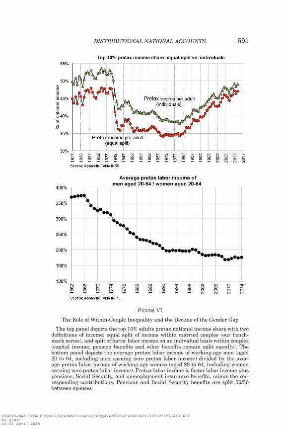
DISTRIBUTIONAL NATIONAL ACCOUNTS 591
FIGURE VI
The Role of Within-Couple Inequality and the Decline of the Gender Gap
The top panel depicts the top 10% adults pretax national income share with twodefinitions of income: equal split of income within married couples (our bench-mark series), and split of factor labor income on an individual basis within couples(capital income, pension benefits and other benefits remain split equally). Thebottom panel depicts the average pretax labor income of working-age men (aged20 to 64, including men earning zero pretax labor income) divided by the aver-age pretax labor income of working-age women (aged 20 to 64, including womenearning zero pretax labor income). Pretax labor income is factor labor income pluspensions, Social Security, and unemployment insurance benefits, minus the cor-responding contributions. Pensions and Social Security benefits are split 50/50between spouses.
Downloaded from https://academic.oup.com/qje/article-abstract/133/2/553/4430651by gueston 01 April 2018

592 QUARTERLY JOURNAL OF ECONOMICS
(+5 points). The gap has declined with the reduction in genderinequality, to about 2 points today. Individualized series thereforeshow a smaller rise in income concentration. The reduction in thegender gap has played an important role in mitigating the rise ofinequality.
The bottom panel of Figure VI quantifies the extent to whichthe gender gap in labor income has shrunk since the 1960s. Wetake the total average pretax labor income of working-age (20–64) men and divide it by the total average pretax labor income ofworking-age women. This measure of the gender gap is larger thanthe one traditionally used—the ratio between men and women’swage conditional on full-time work; see, for example, Blau andKahn (2016)—as it includes not only wage differences conditionalon working, but also differences in labor force participation, hoursof work, fringe benefits, and self-employment income. This is arelevant metric to study overall inequality among adults.57 Menearned 3.7 times more labor income than women in the early 1960sand now earn about 1.75 times more. The gender gap in laborincome has halved but has not disappeared, far from it. Additionalbreakdowns by age—reported in Online Appendix Figure S.7—show that the gender gaps increase with age. Among adults aged20–34, men earn 1.3 times more than women today; the ratioreaches about 2 for adults aged 55 to 64.
In the working-age population (including nonworkers), at themedian, pretax labor income differences between men and womenhave diminished. As shown by the top panel of Figure VII, twoforces are at play. For working-age women, the median pretax in-come has been multiplied by more than five from 1962 to 2014—largely the result of an increase in formal market labor supply—toabout $20,000 today. For working-age men, median pretax laborincome has stagnated: it is the same in 2014 as in 1964, about$35,000. There has been no growth for the median male workerover half a century. The median labor income of men grew rel-atively quickly from 1962 to 1973 and during the 1990s boom,but fell during recessions, effectively erasing all the gains. It col-lapsed, in particular, during the Great Recession, from $40,000in 2007 to $33,000 in 2010. The median labor income of womenhas stopped growing since the late 1990s. For all working-age
57. There is a wide literature on the U.S. gender gap. See, for example, Blau,Ferber, and Winkler (2014) for a classical textbook treatment.
Downloaded from https://academic.oup.com/qje/article-abstract/133/2/553/4430651by gueston 01 April 2018

DISTRIBUTIONAL NATIONAL ACCOUNTS 593
FIGURE VII
Gender Gaps across the Distribution
The top panel shows the median pretax labor income among all working-ageadults (20 to 64), men, and women. Pretax labor income includes pensions, SocialSecurity retirement and disability benefits, and unemployment insurance benefitsand excludes the corresponding contributions. The bottom panel depicts the shareof women in various groups of the distribution of factor labor income. Factor laborincome excludes pensions, Social Security benefits, and unemployment insurancebenefits and is gross of the corresponding contributions. The groups are definedrelative to the full population of adults with positive factor labor income (eitherfrom salaried or nonsalaried work).
Downloaded from https://academic.oup.com/qje/article-abstract/133/2/553/4430651by gueston 01 April 2018

594 QUARTERLY JOURNAL OF ECONOMICS
individuals, as a result, median pretax labor income is only 10%higher in 2014 ($27,500) than 25 years earlier in 1989.
Considerable gender inequalities persist at the top of the dis-tribution. As the bottom panel of Figure VII shows, women arealmost as likely to work as men today. The share of women amongthe population earning positive labor income—from salaried workor self-employment—was 37% in the 1960s and converged to closeto 50% during the 1970s and 1980s: women have closed the par-ticipation gap. But women are much less represented in top laborincome groups. In the 1960s, women accounted for less than 5%of the top 10%, top 1%, and top 0.1% labor income earners. Nowa-days they account for close to 27% of top 10% labor income earners(+22 points), but the increase is smaller the higher one moves upthe distribution, so that the proportion of women in top groupsfalls steeply with income. Women make up only about 16% of thetop 1% labor income earners (+13 points since the 1960s), and11% of the top 0.1% (+9 points). The representation of women atthe very top has only modestly increased since 1999. The glassceiling is not yet close to being shattered.58
V.B. Decomposing Inequality at the Top: Labor versus Capital
Pretax income Y can be decomposed into a labor income com-ponent YL and a capital income component YK. By definition,Y = YL + YK. The share of national income accruing to capitalis α = YK
Y and the labor share is 1 − α = YLY . Our distributional
national accounts make it possible to compute factor shares foreach quantile of the distribution consistent with macroeconomicfactor shares.59 This comprehensive definition of capital income
58. A number of studies have analyzed the share of women in top earningsgroups. Kopczuk, Saez, and Song (2010), Figure X, use Social Security data from1937 to 2004. Because of data limitations, they focus only on commerce and in-dustry employees leaving out all government workers (where women are over-represented particularly in the education sector) and the self-employed. Guvenen,Kaplan, and Song (2014) also use Social Security wage earnings and obtain similarresults. Atkinson, Cesarico, and Voitchovsky (2016) study the share of women intop income groups in a sample of eight countries with individual taxation, but donot consider labor income and capital income separately.
59. To decompose the mixed income of noncorporate businesses into a laborand a capital component, we assume fixed factor shares for simplicity (namely,0.7 for labor income and 0.3 for capital income). This assumption is irrelevant forour results on trends in income levels, income shares, and growth decompositions.It has very little impact on the level and time patterns of capital shares. Weexperimented with other methods to decompose mixed income. For instance, one
Downloaded from https://academic.oup.com/qje/article-abstract/133/2/553/4430651by gueston 01 April 2018
DISTRIBUTIONAL NATIONAL ACCOUNTS 595
is much broader than capital income reported on tax returns. Inparticular, it includes the imputed rents of homeowners, propertytaxes, the returns on pension funds, corporate retained earnings,capital income earned by trusts and estates, and corporate taxes.
For the United States as a whole, the capital share of na-tional income fluctuates around 20% to 30% and has been risingin recent decades, a phenomenon also observed in other countries(Karabarbounis and Neiman 2014; Piketty and Zucman 2014). In2000, 23% of national income was derived from capital; this shareincreased to 30% in 2014. In fact, as shown by Online AppendixTable S.2, almost all the 2000–2014 growth of average nationalincome per adult (0.6% a year on average over this period of time)stems from the rise of capital income: labor income per adult hasgrown by 0.1% per year, while capital income has grown by 2.2%.Corporate retained earnings have increased particularly fast.
The capital share varies widely across the income distribu-tion. The vast majority of Americans earn little capital income.As shown by the top panel of Figure VIII, for the bottom 90%,the capital share is always less than 20%. It has increased overtime, from around 10% from the 1970s to close to 20% today—inlarge part because of the rise of pension funds, which account fora growing share of household wealth (36% in 2014). The capitalshare then rises steeply as one moves up the income distribution.The top 1% derives over half of their incomes from capital, thetop 0.1% more than two thirds today. At the very top, the fluctua-tions in the capital share are spectacular. Early in the twentiethcentury, the top 0.1% derived 70%–80% of its income from capital;this share collapsed during the Great Depression when corporateprofits slumped, before rebounding in the 1950s and 1960s to 90%.In other words, in the post–World War II decades, most top earn-ers derived their income from assets. From the 1970s and 1990s,the fraction of top earners deriving their income from work grew.This process culminated in 2000 when the capital share in the top
can assume the same factor shares in the noncorporate sector as in the corporatesector; or one can attribute to the human capital—education and experience—ofself-employed workers the same return as the one observed for wage earners; orone can attribute to the nonhuman assets used by noncorporate businesses thesame rate of return as the one observed on other assets. This makes very littledifference on the total capital share, see Online Appendix Table I-S.A3.
Downloaded from https://academic.oup.com/qje/article-abstract/133/2/553/4430651by gueston 01 April 2018

596 QUARTERLY JOURNAL OF ECONOMICS
FIGURE VIII
The Capital Share across the Distribution
The top panel depicts the share of capital income in the pretax national incomeof various income groups: full adult population, top 10% incomes, top 1% incomes,and top 0.1% incomes. Total pretax income is the sum of capital income and laborincome so the chart can also be read symmetrically from the top x-axis line as thefraction of labor income in top groups. The bottom panel decomposes the top 1%income share into labor income and capital income.
Downloaded from https://academic.oup.com/qje/article-abstract/133/2/553/4430651by gueston 01 April 2018

DISTRIBUTIONAL NATIONAL ACCOUNTS 597
0.1% reached a low water-mark of 53%. Since then, the capitalshare has bounced back.60
One potential concern with the computation of factor sharesis that the frontier between labor and capital can be fuzzy. Thecapital/labor split can be affected by shifting across tax bases.Is the rise of the capital share—especially at the top—a real phe-nomenon or an illusion caused by changes in tax avoidance? Smithet al. (2017) find that part of S-corporation profits correspond todisguised labor. However, other forms of tax-induced shifting go inthe opposite direction. In all businesses with passive owners—thatis, as long as there is at least one outside investor—active ownershave incentives to pay themselves high wages, as any residualprofit is split across all owners including passive investors. More-over, in all closely held C-corporations, owners have incentives topay themselves high wages too, because the top marginal labor in-come tax rate (43.4% in 2015) is below the top rate on distributedprofits (50.5%). Taking into account all forms of shifting, it is un-clear whether we overstate or understate the capital share.61 Inthis context, we believe it is more justified to follow the stan-dard national accounts labor/capital split in which all profits aretreated as capital income.62
60. As shown by Online Appendix Figure S.33, changes in the age of top earn-ers are consistent with this evolution. The average age of top earners declinedfrom 1979 to 2000, consistent with the notion that the “working rich” were replac-ing capital income earners. Since 2000, this trend has reverted: top earners aregrowing older. The trend break in 2000 mirrors the reversal of the capital share.
61. If anything, it is likely that we underestimate the rise of the capital incomeshare at the top over recent decades. Before the Tax Reform Act of 1986, topmarginal rates on labor income and distributed profits were both high, so thatowners had incentives to pay themselves low wages and low dividends, retainearnings and consume within firms. Part of the high retained earnings we observefrom 1960 to 1985 (3.8% of national income on average) could thus correspondto disguised wages. In Online Appendix Figures S.37 and S.38, we investigatethe effect of treating part of pre-1986 retained earnings as disguised wages. InOnline Appendix Figures S.34, S.35, and S.36, we investigate the effect of treating54% of S-corporation profits as labor income, as advocated by Smith et al. (2017).Because S-corporations profits are only a small part of top 1% income (about 1.5%of national income in recent years) the impact on our capital/labor split at the topis negligible.
62. In Online Appendix Figure S.10, we present another piece of evidence sug-gesting that the rise in the capital share of income is a real economic phenomenon.We compute capital income by assuming a fixed rate of return to capital across thedistribution. This procedure neutralizes potential changes in how labor incomeis reclassified into capital income. The results also show a clear rising share of
Downloaded from https://academic.oup.com/qje/article-abstract/133/2/553/4430651by gueston 01 April 2018

598 QUARTERLY JOURNAL OF ECONOMICS
Capital income has been the key driver of the rise of the top1% income share in the twenty-first century. The bottom panel ofFigure VIII decomposes the top 1% share into labor and capital.The labor income of top 1% earners boomed in the 1980s and1990s, but since the late 1990s it has declined as a fraction ofnational income. Instead, all the increase in the top 1% incomeshare in recent years owes to an upsurge in capital income. Inturn, the key driver of the rise in capital income has been therise in corporate retained earnings—an important macroeconomicphenomenon that could not be studied using individual income taxonly. As shown by Online Appendix Table B.2f, out of the 1.9 pointsincrease in the top 1% pretax income share since 2000, 1.4 pointscome from the rise of retained earnings. These results confirmthe earlier finding from Piketty and Saez (2003) that the rise inincome concentration up to the late 1990s was primarily a laborincome phenomenon; they are also consistent with the more recentfinding by Saez and Zucman (2016) that wealth concentrationhas increased sharply since 2000. The rise in wealth inequalityleads to an increase in capital income concentration, which itselfreinforces wealth inequality as top capital incomes are saved at ahigh rate.
V.C. The Role of Taxes and Transfers
About a third of U.S. national income is redistributed throughtaxes, transfers, and public goods spending. How have changes intaxes and transfers affected the dynamic of posttax income?
1. Taxes. The progressivity of the U.S. tax system hasdeclined significantly over recent decades. The top panel ofFigure IX shows how effective average tax rates vary across theincome distribution.63 The tax rates we compute take into accountall taxes—on individual incomes, payroll, estates, corporate prof-its, properties, and sales—whether levied by federal, state, or localgovernments. Tax rates are computed as a percentage of pretax
capital income at the top, although the increase starts earlier—in the late 1980srather than in the early 2000s.
63. Comprehensive tax rates including all levels of government have beencomputed by Pechman and Okner (1974) for 1966 but long, annual time series ofcomprehensive tax rates had not been computed before. Estimates of federal (butnot state and local) taxes have been produced by the U.S. Congressional BudgetOffice (2016) starting in 1979 and by Piketty and Saez (2007) starting in 1962; noestimates of federal tax rates existed for the pre-1962 period.
Downloaded from https://academic.oup.com/qje/article-abstract/133/2/553/4430651by gueston 01 April 2018
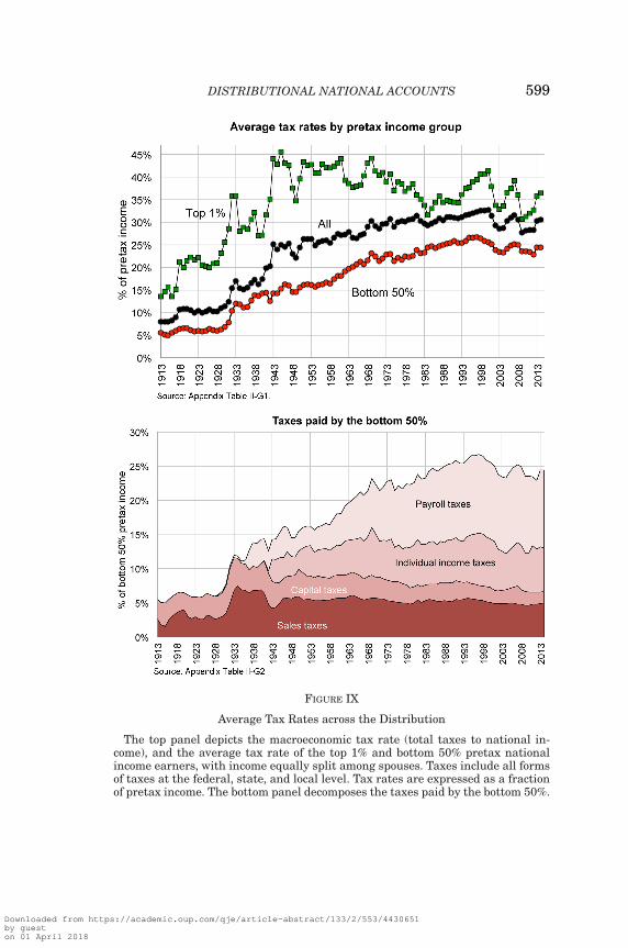
DISTRIBUTIONAL NATIONAL ACCOUNTS 599
FIGURE IX
Average Tax Rates across the Distribution
The top panel depicts the macroeconomic tax rate (total taxes to national in-come), and the average tax rate of the top 1% and bottom 50% pretax nationalincome earners, with income equally split among spouses. Taxes include all formsof taxes at the federal, state, and local level. Tax rates are expressed as a fractionof pretax income. The bottom panel decomposes the taxes paid by the bottom 50%.
Downloaded from https://academic.oup.com/qje/article-abstract/133/2/553/4430651by gueston 01 April 2018

600 QUARTERLY JOURNAL OF ECONOMICS
income. For the United States as a whole, the macroeconomic taxrate increased from 8% in 1913 to 30% in the late 1960s. Sincethen, it has remained at that level. However, effective tax rateshave become more compressed across the income distribution. Inthe 1950s, top 1% income earners paid 40%–45% of their pretaxincome in taxes, while bottom 50% earners paid 15%–20%. Thegap is much smaller today: top earners pay about 30%–35% oftheir income in taxes, while bottom 50% earners pay around 25%.The effective rate paid by the top 1% exhibits cyclical variations.During stock market booms, top 1% income earners realize capitalgains; the taxes paid on those gains are included in the numera-tor of the effective tax rate but the capital gains themselves areexcluded from the denominator, because pretax income (just likenational income) excludes capital gains due to pure price effects.There is, however, a downward trend over time. The bulk of thedecline owes to the fall of corporate and estate taxes. In the 1960s,as shown by Online Appendix Table II-G2, the top 1% paid closeto 20% of its pretax income in corporate and estate taxes while itpays only about 10% today.
The 2013 tax reform has partly reverted the long-run declinein top tax rates. It involved a sizable increase in top marginal in-come tax rates—plus 9.5 points for capital income and 6.5 pointsfor labor income, see Saez (2017)—as a result of surtaxes intro-duced by the Affordable Care Act and the expiration of the 2001Bush tax cuts for top earners. These are the largest hikes in toptax rates since the 1950s, exceeding the 1993 increases of the Clin-ton administration. The effective tax rate paid by top 1% earnershas risen about 4 points between 2011 (32%) and 2013 (36%) andis now back to its level of the early 1980s.64 Although a significantdevelopment, it is worth noting that inequality was much lowerin the 1980s than today, and the long-run decline in corporate andestate taxes continues to exert a downward pressure on effectivetax rates at the top.
While tax rates have tended to fall for top earners since the1960s, they have risen for the bottom 50%. As shown by the bottompanel of Figure IX, this increase essentially derives from the riseof payroll taxes. In the 1960s, payroll taxes amounted to 5% of thepretax income of bottom 50% earners; today they exceed 10%. Infact, payroll taxes are now much more important than any other
64. The U.S. Congressional Budget Office (2016) also finds an increase byabout 4–5 points in the federal tax rate of the top 1% from 2011 to 2013.
Downloaded from https://academic.oup.com/qje/article-abstract/133/2/553/4430651by gueston 01 April 2018

DISTRIBUTIONAL NATIONAL ACCOUNTS 601
taxes—federal and state—borne by the bottom 50%. In 2014, pay-roll taxes amount to 11.3% of pretax income, significantly abovethe next largest items—federal and state income taxes, 6.6% ofpretax income, and sales taxes, 4.7%.65 Although payroll taxes fi-nance transfers—Social Security and Medicare—that go in partto the bottom 50%, their increase contributes to the stagnation ofthe posttax income of working-age bottom 50% Americans.
2. Transfers. One major evolution in the U.S. economy overthe past 50 years is the rise of individualized transfers—monetaryand more importantly in-kind. While public goods spending hasremained constant around 18% of national income, transfers—other than Social Security, disability, and unemployment insur-ance, which are already included in pretax income—have in-creased from about 2% of national income in 1960 to close to 11%today; see Online Appendix Figure S.12 and Online Appendix Ta-ble I-S.A11. The two largest transfers are Medicare (4% of nationalincome in 2014) and Medicaid (3.4%); other important transfersinclude refundable tax credits (0.8%), veterans’ benefits (0.6%),and food stamps (0.5%).
Overall, individualized transfers tend to be targeted to themiddle class. The top panel of Figure X shows the average trans-fer received by posttax income groups, expressed as a percent ofthe average national income in the full adult population.66 DespiteMedicaid and other means-tested programs which entirely go tothe bottom 50%, the middle 40% receives larger transfers than thebottom 50% Americans, in particular because Medicare largelygoes to the middle-class. In 2014, the bottom 50% received theequivalent of 10.5% of per-adult national income, the middle-classreceived more—14%—and the top 10% received less—about 8%.As shown by Online Appendix Figure S.13, there is a similar pat-tern when including Social Security benefits: the average transferthen amounts to close to 17% of average income, and 23% for themiddle 40%.
65. In keeping with the national accounts conventions, we treat the nonrefund-able portion of tax credits and tax deductions as negative taxes, but the refundableportion of tax credits as a transfer. As a result, nobody can have negative incometaxes.
66. We choose this representation for transfers because individualized trans-fers are fairly close to a fixed amount per individual, in contrast to taxes whichare fairly close to being proportional to pretax income.
Downloaded from https://academic.oup.com/qje/article-abstract/133/2/553/4430651by gueston 01 April 2018

602 QUARTERLY JOURNAL OF ECONOMICS
FIGURE X
The Role of Transfers
The top panel depicts average individualized transfers received by posttax na-tional income groups, expressed as a percent of the average national income in thefull adult population. These transfers exclude Social Security retirement and dis-ability benefits, and unemployment insurance benefits. The bottom panel depictsthe average posttax income of the middle 40% (top 50% excluding the top 10%),including versus excluding all transfers (individualized transfers and public goodsspending).
Downloaded from https://academic.oup.com/qje/article-abstract/133/2/553/4430651by gueston 01 April 2018

DISTRIBUTIONAL NATIONAL ACCOUNTS 603
The middle class appears as the main winner of redistribu-tion: while it receives growing individualized transfers, its effec-tive tax rate has remained stable at around 30% since the late1960s. Transfers have played a key role in enabling its income togrow in recent years. As shown by the bottom panel of Figure X,without transfers average income for the middle 40% would nothave grown at all from 1999 to 2014. In fact it grew 8%, thanks toan increase of 32% in transfers received excluding Social Security.Tax credits—the 2008 Economic Stimulus Payments, the Amer-ican Opportunity Tax Credit, the Making Work Pay Tax Credit,and Health Insurance Premium Assistance Credits (in the contextof the Affordable Care Act)—played a particularly important roleduring the Great Recession. Without transfers the average incomeof the middle class would have fallen by 11% between 2007 and2009; thanks to transfers the decline was limited to 3%.
In contrast, given the dynamic in their pretax income, trans-fers have not been sufficient to enable bottom 50% incomes to growsignificantly. As shown by Online Appendix Figure S.4, between1999 and 2014, the posttax income of the bottom 50% excluding to-tal transfers (individualized and collective) collapsed from $9,900to $6,600; transfers were just enough to maintain posttax incomeconstant at around $25,000.
VI. CONCLUSION
In this article, we have combined tax, survey, and nationalaccounts data to build distributional national accounts for theUnited States since 1913. Our series capture 100% of nationalincome. They can be used to provide decompositions of growth byincome groups consistent with macroeconomic growth; to quantifyhow government intervention shapes inequality by contrastingpretax and posttax income; to assess the effect of gender inequalityon the overall distribution of income; to study how factor sharesvary across the income spectrum; and to simulate the growth anddistributional impacts of tax and transfer reforms. As inequalityhas become a key issue in the public debate in the United States,we feel that such distributional national accounts are a neededtool to better monitor economic growth and its distribution. Wesee three main avenues for future research.
First, our data set should be seen as a prototype to be furtherdeveloped and improved on—just like the national accounts them-selves are regularly improved. Looking forward, our assumptions
Downloaded from https://academic.oup.com/qje/article-abstract/133/2/553/4430651by gueston 01 April 2018
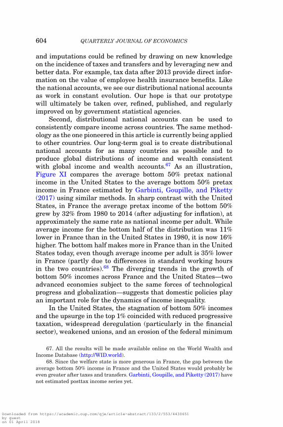
604 QUARTERLY JOURNAL OF ECONOMICS
and imputations could be refined by drawing on new knowledgeon the incidence of taxes and transfers and by leveraging new andbetter data. For example, tax data after 2013 provide direct infor-mation on the value of employee health insurance benefits. Likethe national accounts, we see our distributional national accountsas work in constant evolution. Our hope is that our prototypewill ultimately be taken over, refined, published, and regularlyimproved on by government statistical agencies.
Second, distributional national accounts can be used toconsistently compare income across countries. The same method-ology as the one pioneered in this article is currently being appliedto other countries. Our long-term goal is to create distributionalnational accounts for as many countries as possible and toproduce global distributions of income and wealth consistentwith global income and wealth accounts.67 As an illustration,Figure XI compares the average bottom 50% pretax nationalincome in the United States to the average bottom 50% pretaxincome in France estimated by Garbinti, Goupille, and Piketty(2017) using similar methods. In sharp contrast with the UnitedStates, in France the average pretax income of the bottom 50%grew by 32% from 1980 to 2014 (after adjusting for inflation), atapproximately the same rate as national income per adult. Whileaverage income for the bottom half of the distribution was 11%lower in France than in the United States in 1980, it is now 16%higher. The bottom half makes more in France than in the UnitedStates today, even though average income per adult is 35% lowerin France (partly due to differences in standard working hoursin the two countries).68 The diverging trends in the growth ofbottom 50% incomes across France and the United States—twoadvanced economies subject to the same forces of technologicalprogress and globalization—suggests that domestic policies playan important role for the dynamics of income inequality.
In the United States, the stagnation of bottom 50% incomesand the upsurge in the top 1% coincided with reduced progressivetaxation, widespread deregulation (particularly in the financialsector), weakened unions, and an erosion of the federal minimum
67. All the results will be made available online on the World Wealth andIncome Database (http://WID.world).
68. Since the welfare state is more generous in France, the gap between theaverage bottom 50% income in France and the United States would probably beeven greater after taxes and transfers. Garbinti, Goupille, and Piketty (2017) havenot estimated posttax income series yet.
Downloaded from https://academic.oup.com/qje/article-abstract/133/2/553/4430651by gueston 01 April 2018
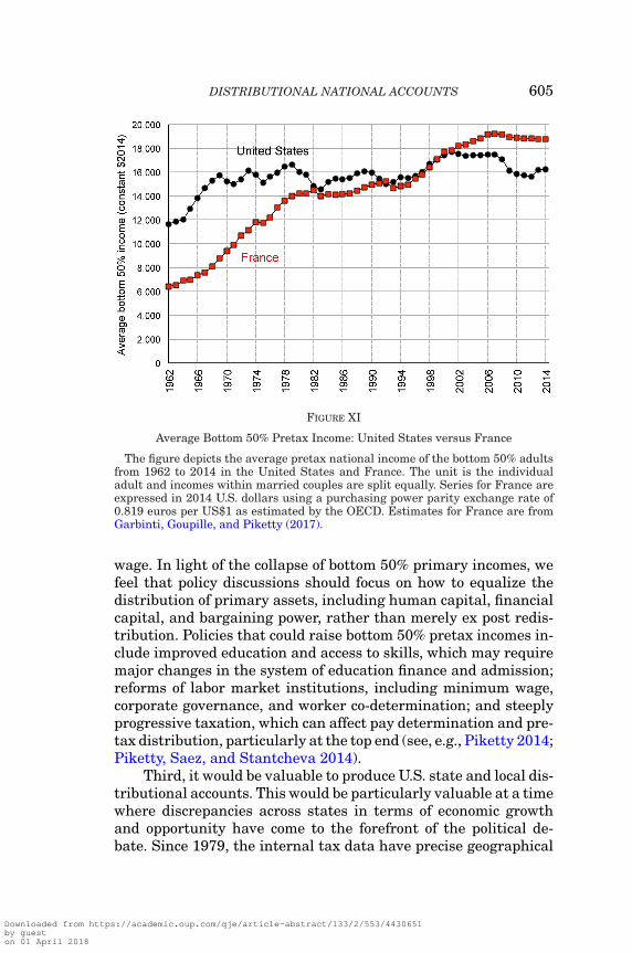
DISTRIBUTIONAL NATIONAL ACCOUNTS 605
FIGURE XI
Average Bottom 50% Pretax Income: United States versus France
The figure depicts the average pretax national income of the bottom 50% adultsfrom 1962 to 2014 in the United States and France. The unit is the individualadult and incomes within married couples are split equally. Series for France areexpressed in 2014 U.S. dollars using a purchasing power parity exchange rate of0.819 euros per US$1 as estimated by the OECD. Estimates for France are fromGarbinti, Goupille, and Piketty (2017).
wage. In light of the collapse of bottom 50% primary incomes, wefeel that policy discussions should focus on how to equalize thedistribution of primary assets, including human capital, financialcapital, and bargaining power, rather than merely ex post redis-tribution. Policies that could raise bottom 50% pretax incomes in-clude improved education and access to skills, which may requiremajor changes in the system of education finance and admission;reforms of labor market institutions, including minimum wage,corporate governance, and worker co-determination; and steeplyprogressive taxation, which can affect pay determination and pre-tax distribution, particularly at the top end (see, e.g., Piketty 2014;Piketty, Saez, and Stantcheva 2014).
Third, it would be valuable to produce U.S. state and local dis-tributional accounts. This would be particularly valuable at a timewhere discrepancies across states in terms of economic growthand opportunity have come to the forefront of the political de-bate. Since 1979, the internal tax data have precise geographical
Downloaded from https://academic.oup.com/qje/article-abstract/133/2/553/4430651by gueston 01 April 2018

606 QUARTERLY JOURNAL OF ECONOMICS
indicators and are large enough to study state-level outcomes. Ourapproach naturally lends itself to the definition of national incomeacross geographical units by considering the individual nationalincome of residents in each geographical unit.69 Starting in 1996,the population-wide tax data could be leveraged to construct mea-sures of national income at an even finer geographical level, suchas the county or the metropolitan statistical area.
PARIS SCHOOL OF ECONOMICS
UNIVERSITY OF CALIFORNIA, BERKELEY,AND NATIONAL BUREAU OF ECONOMIC RESEARCH
UNIVERSITY OF CALIFORNIA, BERKELEY,AND NATIONAL BUREAU OF ECONOMIC RESEARCH
SUPPLEMENTARY MATERIAL
An Online Appendix for this article can be found at The Quar-terly Journal of Economics online. Data replicating tables andfigures in this article can be found in Piketty, Saez, and Zuc-man (2017) in the Harvard Dataverse, doi:10.7910/DVN/SLXCUJ.Data files are also available at http://gabriel-zucman.eu/usdina.
REFERENCES
Alstadsæter, Annette, Niels Johannesen, and Gabriel Zucman, “Tax Evasion andInequality,” NBER Working Paper 23772, 2017a.
———, “Who Owns the Wealth in Tax Havens? Macro Evidence and Implicationsfor Global Inequality,” NBER Working Paper 23805, 2017b.
Alvaredo, Facundo, Anthony Atkinson, Thomas Piketty, Emmanuel Saez, andGabriel Zucman, The World Wealth and Income Database, http://www.wid.world, 2011–2017.
Alvaredo, Facundo, Anthony Atkinson, Lucas Chancel, Thomas Piketty, Em-manuel Saez, and Gabriel Zucman, “Distributional National Accounts (DINA)Guidelines: Concepts and Methods Used in the World Wealth and IncomeDatabase,” WID Working Paper 2016/1, 2016.
Armour, Philip, Richard V. Burkhauser, and Jeffrey Larrimore, “Levels and Trendsin United States Income and Its Distribution: A Crosswalk from Market In-come towards a Comprehensive Haig-Simons Income Measure,” Southern Eco-nomic Journal, 81 (2014), 271–293
Atkinson, Anthony B, “Top Incomes in the UK over the 20th Century,” Journal ofthe Royal Statistical Society: Series A, 168 (2005), 325–343
Atkinson, Anthony B, Alessandra Cesarico, and Sarah Voitchovsky, “Top Incomesand the Gender Divide,” LSE International Inequality Institute Working Pa-per 5, 2016.
69. National accounts provide measures of GDP, personal consumption expen-diture, and personal income (but not national income) at the state level (see U.S.Department of Commerce, Bureau of Economic Analysis, 2016).
Downloaded from https://academic.oup.com/qje/article-abstract/133/2/553/4430651by gueston 01 April 2018

DISTRIBUTIONAL NATIONAL ACCOUNTS 607
Atkinson, Anthony B., and John Micklewright, “On the Reliability of Income Datain the Family Expenditure Survey,” Journal of the Royal Statistical Society,Series A, 146 (1983), 33–61.
Atkinson, Anthony, Thomas Piketty, and Emmanuel Saez, “Top Incomes in theLong-Run of History,” Journal of Economic Literature, 49 (2011), 3–71.
Atkinson, Anthony B., Lee Rainwater, and Timothy M. Smeeding, “Income Distri-bution in OECD Countries,” OECD Social Policy Studies No. 18, 1995.
Australian Bureau of Statistics, “Australian National Accounts: Distribution ofHousehold Income, Consumption and Wealth, 2009–10,” 2015, available on-line at http://www.abs.gov.au/ausstats/[email protected]/mf/5204.0.55.009#.
Auten, Gerald, and David Splinter, “Income Inequality in the United States: UsingTax Data to Measure Long-term Trends,” Mimeo, U.S. Department of theTreasury, Office of Tax Analysis, 2017.
Barnett, G. E., Two Tracts by Gregory King (Baltimore: Johns Hopkins UniversityPress, 1936).
Blau, Francinne, Marianne A. Ferber, and Anne E. Winkler. The Economics ofWomen, Men, and Work, 7th ed. (Upper Saddle River, NJ: Prentice Hall, 2014).
Blau, Francinne, and Lawrence M. Kahn, “The Gender Wage Gap: Extent, Trends,and Explanations,” NBER Working Paper 21913, 2016.
Boskin, Michael, “Toward a More Accurate Measure of the Cost of Living,” Reportto the Senate Finance Committee from the Advisory Commission to Study theConsumer Price Index, 1996.
Chiappori, Pierre-Andre, and Costas Meghir, “Intrahousehold Inequality,” inHandbook of Income Distribution, Anthony B. Atkinson and Francois Bour-guignon eds. (Amsterdam: Elsevier, 2015), 1369–1418.
Cohn, D’Vera, Jeffrey S. Passel, Wendy Wang, and Gretchen Livingston, “BarelyHalf of U.S. Adults Are Married—A Record Low,” Pew Research Center, 2011.
Currie, Janet, “U.S. Food and Nutrition Programs,” in Means-Tested Transfer Pro-grams in the United States, Robert Moffitt, ed. (Chicago: University of ChicagoPress, 2003).
Deaton, Angus, “Measuring Poverty in a Growing World (or Measuring Growth ina Poor World),” Review of Economics and Statistics, 87 (2005), 1–19.
Fesseau, Maryse, and Maria Liviana Mattonetti, “Distributional Measures acrossHousehold Groups in a National Accounts Framework: Results from an Ex-perimental Cross-Country Exercise on Household Income, Consumption andSaving,” OECD Statistics Working Paper, 2013.
Fesseau, Maryse, Florence Wolff, and Maria Liviana Mattonetti, “A Cross Coun-try Comparison of Household Income, Consumption and Wealth between Mi-cro Sources and National Accounts Aggregates,” OECD Working Paper 52,2013.
Finkelstein, Amy, Nathaniel Hendren, and Erzo F. P. Luttmer, “The Value of Med-icaid: Interpreting Results from the Oregon Health Insurance Experiment,”NBER Working Paper 21308, 2016.
Fixler, Dennis, and David S. Johnson, “Accounting for the Distribution of Income inthe U.S. National Accounts,” in Measuring Economic Stability and Progress,D. Jorgenson, J. S. Landefeld, and P. Schreyer, eds. (Chicago: University ofChicago Press), 2014.
Fixler, Dennis, David Johnson, Andrew Craig, and Kevin Furlong, “A ConsistentData Series to Evaluate Growth and Inequality in the National Accounts,”BEA Working Paper, 2015.
Fullerton, Don, and Gilbert E. Metcalf, “Tax Incidence,” in Handbook of PublicEconomics, Volume 4, A. J. Auerbach and M. Feldstein, eds. (Amsterdam:North-Holland, 2002), 1787–1872.
Furlong, Kevin, “Distributional Estimates in the U.S. National Accounts:Integrating Micro and Macro Data,” Bureau of Economic Analysis,ftp://ftp.census.gov/adrm/fesac/2014-06-13_furlong.pdf, 2014.
Garbinti, Bertrand, Jonathan Goupille, and Thomas Piketty, “Inequality Dynam-ics in France, 1900–2014: Evidence from Distributional National Accounts(DINA),” WID Working Paper 4/2017, 2017.
Downloaded from https://academic.oup.com/qje/article-abstract/133/2/553/4430651by gueston 01 April 2018

608 QUARTERLY JOURNAL OF ECONOMICS
Guvenen, Fatih, Greg Kaplan, and Jae Song, “The Glass Ceiling and the PaperFloor: Gender Differences among Top Earners, 1981–2012,” NBER WorkingPaper 20560, 2014.
Harberger, Arnold C., “The Incidence of the Corporation Income Tax,” Journal ofPolitical Economy, 70 (1962), 215–240.
Karabarbounis, Loukas, and Brent Neiman, “The Global Decline of the LaborShare,” Quarterly Journal of Economics, 129 (2014), 61–103
Katz, Lawrence, and David Autor, “Changes in the Wage Structure and EarningsInequality,” in Handbook of Labor Economics, Volume 3A, O. Ashenfelter andD. Card, eds. (Amsterdam: North-Holland, 1999).
Katz, Lawrence, and Kevin Murphy, “Changes in Relative Wages, 1963–1987:Supply and Demand Factors,” Quarterly Journal of Economics 107 (1992),35–78.
King, Willford I., The Wealth and Income of the People of the United States (NewYork: Macmillan, 1915).
———, “Wealth Distribution in the Continental United States at the Close of1921,” Journal of the American Statistical Association, 22 (1927), 135–153.
———, The National Income and Its Purchasing Power (New York: National Bu-reau of Economic Research, 1930).
Kopczuk, Wojciech, Emmanuel Saez, and Jae Song, “Earnings Inequality and Mo-bility in the United States: Evidence from Social Security Data since 1937,”Quarterly Journal of Economics, 125 (2010), 91–128.
Kuznets, Simon, National Income and Its Composition, 1919–1938 (New York:National Bureau of Economic Research, 1941).
———, Shares of Upper Income Groups in Income and Savings (New York: Na-tional Bureau of Economic Research), 1953.
Lakner, Christoph, and Branko Milanovic, “Global Income Distribution: From theFall of the Berlin Wall to the Great Recession,” World Bank Policy ResearchWorking Paper 6719, 2013.
McCully, Clinton, “Integration of Micro and Macro data on Consumer Income andExpenditure,” in Measuring Economic Stability and Progress, D. Jorgenson,J. S. Landefeld and P. Schreyer, eds. (Chicago: University of Chicago Press,2014).
Meyer, Bruce D., and James X. Sullivan, “Consumption and Income Inequality inthe U.S. since the 1960s,” NBER Working Paper 23655, 2017.
Monaco, Kristan, and Brooks Pierce, “Compensation Inequality: Evidence fromthe National Compensation Survey,” Monthly Labor Review (July 2015).
Pechman, Joseph A., and Benjamin A. Okner, Who Bears the Tax Burden? (Wash-ington, DC: Brookings Institution Press, 1974).
Pierce, Brooks, “Compensation Inequality, 1913–1998,” Quarterly Journal of Eco-nomics, 116 (2001), 1493–1525
Piketty, Thomas, Les hauts revenus en France au XXe siecle: Inegalites et redistri-butions 1901–1998 (Paris: Grasset, 2001).
———, “Income Inequality in France, 1901–1998,” Journal of Political Economy,111 (2003), 1004–1042
———, Capital in the 21st Century (Cambridge, MA: Harvard University Press,2014).
Piketty, Thomas, and Emmanuel Saez, “Income Inequality in the United States,1913–1998,” Quarterly Journal of Economics, 118 (2003), 1–39
———, “How Progressive is the U.S. Federal Tax System? A Historical andInternational Perspective,” Journal of Economic Perspectives, 21 (2007),3–24.
Piketty, Thomas, Emmanuel Saez, and Gabriel Zucman, “Replication Data for:‘Distributional Accounts: Methods and Estimates for the United States’,” Har-vard Dataverse (2017), doi:10.7910/DVN/SLXCUJ.
Piketty, Thomas, Emmanuel Saez, and Stefanie Stantcheva, “Optimal Taxation ofTop Labor Incomes: A Tale of Three Elasticities,” American Economic Journal:Economic Policy, 6 (2014), 230–271.
Downloaded from https://academic.oup.com/qje/article-abstract/133/2/553/4430651by gueston 01 April 2018

DISTRIBUTIONAL NATIONAL ACCOUNTS 609
Piketty, Thomas, Li Yang, and Gabriel Zucman, “Capital Accumulation, PrivateProperty, and Rising Income Inequality in China, 1978–2015,” NBER WorkingPaper 23368, 2017.
Piketty, Thomas, and Gabriel Zucman, “Capital Is Back: Wealth-Income Ratiosin Rich Countries, 1700–2010,” Quarterly Journal of Economics, 129 (2014),1255–1310.
Saez, Emmanuel, “Striking It Richer: The Evolution of Top Incomes in the UnitedStates,” Pathways Magazine, Stanford Center for the Study of Poverty andInequality, 6–7, 2008.
———, “Statistics of Income Tabulations: High Incomes, Gender, Age, EarningsSplit, and Nonfilers,” SOI Working Paper, 2016.
———, “Taxing the Rich More: Preliminary Evidence from the 2013 Tax Increase,”Tax Policy and the Economy, Volume 31, Robert Moffitt, ed. (Cambridge, MA:MIT Press, 2017).
Saez, Emmanuel, and Zucman Gabriel, “Wealth Inequality in the United Statessince 1913: Evidence from Capitalized Income Tax Data,” Quarterly Journalof Economics, 131 (2016), 519–578.
Sala-i-Martin, Xavier, “The World Distribution of Income: Falling Poverty and...Convergence, Period,” Quarterly Journal of Economics, 121 (2006), 351–397.
Smith, Matthew, Danny Yagan, Owen Zidar, and Eric Zwick, “Capitalists inthe Twenty-First Century,” UC Berkeley and University of Chicago WorkingPaper, 2017.
Stiglitz, Joseph, Amartya Sen, and Jean-Paul Fitoussi, Report by the Commissionon the Measurement of Economic Performance and Social Progress, INSEE,www.stiglitz-sen-fitoussi.fr, 2009.
United Nations, “System of National Accounts 2008,” European Com-munities, International Monetary Fund, Organisation for EconomicCo-operation and Development, United Nations, and World Bank,http://unstats.un.org/unsd/nationalaccount/docs/SNA2008.pdf, 2009.
U.S. Board of Governors of the Federal Reserve System, “Z.1 Financial Accountsof the United States , Fourth Quarter 2013,” March 6, 2014.
U.S. Census Bureau, “Income and Poverty in the United States: 2015 CurrentPopulation Reports,” Publication P60-252, Census Bureau, 2016.
U.S. Congressional Budget Office, “The Distribution of Household Income andFederal Taxes, 2013,” Congressional Budget Office Report, 2016.
U.S. Department of CommerceBureau of Economic Analysis, National Income andProduct Accounts of the United States, 1929–2015 (Washington, U.S. Depart-ment of Commerce, 2016).
U.S. Treasury Department, Internal Revenue Service, Statistics of Income: In-dividual Income Tax Returns (Washington, U.S. Treasury Department 1916-present).
Zucman, Gabriel, “The Missing Wealth of Nations: Are Europe and the U.S. NetDebtors or Net Creditors?,” Quarterly Journal of Economics, 128 (2013), 1321–1364.
———, “Taxing across Borders: Tracking Personal Wealth and Corporate Profits,”Journal of Economic Perspectives, 28 (2014), 121–148.
Downloaded from https://academic.oup.com/qje/article-abstract/133/2/553/4430651by gueston 01 April 2018
Related Documents


![QUARTERLY JOURNAL OF ECONOMICS - … · The Quarterly Journal of Economics, ... Hastorf and Cantril [1954] examine student perceptions of a contentious football game be- tween Princeton](https://static.cupdf.com/doc/110x72/5b5fab827f8b9a415d8e71e9/quarterly-journal-of-economics-the-quarterly-journal-of-economics-hastorf.jpg)


