arXiv:1606.06687v2 [hep-th] 20 Sep 2016 Preprint typeset in JHEP style - HYPER VERSION January 2016 The Quantum Hall Effect TIFR Infosys Lectures David Tong Department of Applied Mathematics and Theoretical Physics, Centre for Mathematical Sciences, Wilberforce Road, Cambridge, CB3 OBA, UK http://www.damtp.cam.ac.uk/user/tong/qhe.html [email protected] –1–

Welcome message from author
This document is posted to help you gain knowledge. Please leave a comment to let me know what you think about it! Share it to your friends and learn new things together.
Transcript

arX
iv:1
606.
0668
7v2
[he
p-th
] 2
0 Se
p 20
16
Preprint typeset in JHEP style - HYPER VERSION January 2016
The Quantum Hall EffectTIFR Infosys Lectures
David Tong
Department of Applied Mathematics and Theoretical Physics,
Centre for Mathematical Sciences,
Wilberforce Road,
Cambridge, CB3 OBA, UK
http://www.damtp.cam.ac.uk/user/tong/qhe.html
– 1 –

Abstract:
There are surprisingly few dedicated books on the quantum Hall effect. Two prominent
ones are
• Prange and Girvin, “The Quantum Hall Effect”
This is a collection of articles by most of the main players circa 1990. The basics are
described well but there’s nothing about Chern-Simons theories or the importance of
the edge modes.
• J. K. Jain, “Composite Fermions”
As the title suggests, this book focuses on the composite fermion approach as a lens
through which to view all aspects of the quantum Hall effect. It has many good
explanations but doesn’t cover the more field theoretic aspects of the subject.
There are also a number of good multi-purpose condensed matter textbooks which
contain extensive descriptions of the quantum Hall effect. Two, in particular, stand
out:
• Eduardo Fradkin, Field Theories of Condensed Matter Physics
• Xiao-Gang Wen, Quantum Field Theory of Many-Body Systems: From the Origin
of Sound to an Origin of Light and Electrons
Several excellent lecture notes covering the various topics discussed in these lec-
tures are available on the web. Links can be found on the course webpage:
http://www.damtp.cam.ac.uk/user/tong/qhe.html.

Contents
1. The Basics 5
1.1 Introduction 5
1.2 The Classical Hall Effect 6
1.2.1 Classical Motion in a Magnetic Field 6
1.2.2 The Drude Model 7
1.3 Quantum Hall Effects 10
1.3.1 Integer Quantum Hall Effect 11
1.3.2 Fractional Quantum Hall Effect 13
1.4 Landau Levels 14
1.4.1 Landau Gauge 18
1.4.2 Turning on an Electric Field 21
1.4.3 Symmetric Gauge 22
1.5 Berry Phase 27
1.5.1 Abelian Berry Phase and Berry Connection 28
1.5.2 An Example: A Spin in a Magnetic Field 32
1.5.3 Particles Moving Around a Flux Tube 35
1.5.4 Non-Abelian Berry Connection 38
2. The Integer Quantum Hall Effect 42
2.1 Conductivity in Filled Landau Levels 42
2.1.1 Edge Modes 44
2.2 Robustness of the Hall State 48
2.2.1 The Role of Disorder 48
2.2.2 The Role of Gauge Invariance 51
2.2.3 An Aside: The Kubo Formula 54
2.2.4 The Role of Topology 57
2.3 Particles on a Lattice 61
2.3.1 TKNN Invariants 61
2.3.2 The Chern Insulator 65
2.3.3 Particles on a Lattice in a Magnetic Field 66
– 1 –

3. The Fractional Quantum Hall Effect 74
3.1 Laughlin States 76
3.1.1 The Laughlin Wavefunction 76
3.1.2 Plasma Analogy 80
3.1.3 Toy Hamiltonians 83
3.2 Quasi-Holes and Quasi-Particles 85
3.2.1 Fractional Charge 88
3.2.2 Introducing Anyons 90
3.2.3 Fractional Statistics 92
3.2.4 Ground State Degeneracy and Topological Order 97
3.3 Other Filling Fractions 99
3.3.1 The Hierarchy 100
3.3.2 Composite Fermions 101
3.3.3 The Half-Filled Landau Level 106
3.3.4 Wavefunctions for Particles with Spin 110
4. Non-Abelian Quantum Hall States 114
4.1 Life in Higher Landau Levels 114
4.2 The Moore-Read State 116
4.2.1 Quasi-Holes 118
4.2.2 Majorana Zero Modes 123
4.2.3 Read-Rezayi States 129
4.3 The Theory of Non-Abelian Anyons 131
4.3.1 Fusion 132
4.3.2 The Fusion Matrix 135
4.3.3 Braiding 139
4.3.4 There is a Subject Called Topological Quantum Computing 142
5. Chern-Simons Theories 143
5.1 The Integer Quantum Hall Effect 144
5.1.1 The Chern-Simons Term 146
5.1.2 An Aside: Periodic Time Makes Things Hot 148
5.1.3 Quantisation of the Chern-Simons level 150
5.2 The Fractional Quantum Hall Effect 153
5.2.1 A First Look at Chern-Simons Dynamics 154
5.2.2 The Effective Theory for the Laughlin States 156
5.2.3 Chern-Simons Theory on a Torus 161
5.2.4 Other Filling Fractions and K-Matrices 163
– 2 –

5.3 Particle-Vortex Duality 167
5.3.1 The XY -Model and the Abelian-Higgs Model 167
5.3.2 Duality and the Chern-Simons Ginzburg-Landau Theory 171
5.3.3 Composite Fermions and the Half-Filled Landau Level 177
5.4 Non-Abelian Chern-Simons Theories 181
5.4.1 Introducing Non-Abelian Chern-Simons Theories 181
5.4.2 Canonical Quantisation and Topological Order 183
5.4.3 Wilson Lines 185
5.4.4 Chern-Simons Theory with Wilson Lines 189
5.4.5 Effective Theories of Non-Abelian Quantum Hall States 197
6. Edge Modes 198
6.1 Laughlin States 198
6.1.1 The View from the Wavefunction 198
6.1.2 The View from Chern-Simons Theory 200
6.1.3 The Chiral Boson 205
6.1.4 Electrons and Quasi-Holes 207
6.1.5 Tunnelling 212
6.2 The Bulk-Boundary Correspondence 214
6.2.1 Recovering the Laughlin Wavefunction 214
6.2.2 Wavefunction for Chern-Simons Theory 218
6.3 Fermions on the Boundary 223
6.3.1 The Free Fermion 223
6.3.2 Recovering the Moore-Read Wavefunction 226
6.4 Looking Forwards: More Conformal Field Theory 228
– 3 –

Acknowledgements
These lectures were given in TIFR, Mumbai. I’m grateful to the students, postdocs,
faculty and director for their excellent questions and comments which helped me a lot
in understanding what I was saying.
To first approximation, these lecture notes contain no references to original work. I’ve
included some footnotes with pointers to review articles and a handful of key papers.
More extensive references can be found in the review articles mentioned earlier, or in
the book of reprints, “Quantum Hall Effect”, edited by Michael Stone.
My thanks to everyone in TIFR for their warm hospitality. Thanks also to Bart
Andrews for comments and typo-spotting. These lecture notes were written as prepa-
ration for research funded by the European Research Council under the European
Unions Seventh Framework Programme (FP7/2007-2013), ERC grant agreement STG
279943, “Strongly Coupled Systems”.
Magnetic Scales
Cyclotron Frequency: ωB =eB
m
Magnetic Length: lB =
√
~
eB
Quantum of Flux: Φ0 =2π~
e
Hall Resistivity: ρxy =2π~
e21
ν
– 4 –

1. The Basics
1.1 Introduction
Take a bunch of electrons, restrict them to move in a two-dimensional plane and turn
on a strong magnetic field. This simple set-up provides the setting for some of the most
wonderful and surprising results in physics. These phenomena are known collectively
as the quantum Hall effect.
The name comes from the most experimentally visible of these surprises. The Hall
conductivity (which we will define below) takes quantised values
σxy =e2
2π~ν
Originally it was found that ν is, to extraordinary precision, integer valued. Of course,
we’re very used to things being quantised at the microscopic, atomic level. But this
is something different: it’s the quantisation of an emergent, macroscopic property in
a dirty system involving many many particles and its explanation requires something
new. It turns out that this something new is the role that topology can play in quantum
many-body systems. Indeed, ideas of topology and geometry will be a constant theme
throughout these lectures.
Subsequently, it was found that ν is not only restricted to take integer values, but can
also take very specific rational values. The most prominent fractions experimentally
are ν = 1/3 and ν = 2/5 but there are many dozens of different fractions that have
been seen. This needs yet another ingredient. This time, it is the interactions between
electrons which result in a highly correlated quantum state that is now recognised as a
new state of matter. It is here that the most remarkable things happen. The charged
particles that roam around these systems carry a fraction of the charge of the electron,
as if the electron has split itself into several pieces. Yet this occurs despite the fact
that the electron is (and remains!) an indivisible constituent of matter.
In fact, it is not just the charge of the electron that fractionalises: this happens to the
“statistics” of the electron as well. Recall that the electron is a fermion, which means
that the distribution of many electrons is governed by the Fermi-Dirac distribution
function. When the electron splits, so too does its fermionic nature. The individual
constituents are no longer fermions, but neither are they bosons. Instead they are new
entities known as anyons which, in the simplest cases, lie somewhere between bosons
and fermions. In more complicated examples even this description breaks down: the
resulting objects are called non-Abelian anyons and provide physical embodiment of
the kind of non-local entanglement famous in quantum mechanics.
– 5 –

Because of this kind of striking behaviour, the quantum Hall effect has been a con-
stant source of new ideas, providing hints of where to look for interesting and novel
phenomena, most of them related to the ways in which the mathematics of topology
impinges on quantum physics. Important examples include the subject of topological
insulators, topological order and topological quantum computing. All of them have
their genesis in the quantum Hall effect.
Underlying all of these phenomena is an impressive theoretical edifice, which involves
a tour through some of the most beautiful and important developments in theoretical
and mathematical physics over the past decades. The first attack on the problem fo-
cussed on the microscopic details of the electron wavefunctions. Subsequent approaches
looked at the system from a more coarse-grained, field-theoretic perspective where a
subtle construction known as Chern-Simons theory plays the key role. Yet another
perspective comes from the edge of the sample where certain excitations live that know
more about what’s happening inside than you might think. The main purpose of these
lectures is to describe these different approaches and the intricate and surprising links
between them.
1.2 The Classical Hall Effect
The original, classical Hall effect was discovered in 1879 by Edwin Hall. It is a simple
consequence of the motion of charged particles in a magnetic field. We’ll start these
lectures by reviewing the underlying physics of the Hall effect. This will provide a
useful background for our discussion of the quantum Hall effect.
Here’s the set-up. We turn on a constant mag-
xIHV
B
Figure 1: The classical Hall ef-
fect
netic field, B pointing in the z-direction. Meanwhile,
the electrons are restricted to move only in the (x, y)-
plane. A constant current I is made to flow in the
x-direction. The Hall effect is the statement that
this induces a voltage VH (H is for “Hall”) in the
y-direction. This is shown in the figure to the right.
1.2.1 Classical Motion in a Magnetic Field
The Hall effect arises from the fact that a magnetic field causes charged particles to
move in circles. Let’s recall the basics. The equation of motion for a particle of mass
m and charge −e in a magnetic field is
mdv
dt= −ev ×B
– 6 –

When the magnetic field points in the z-direction, so thatB = (0, 0, B), and the particle
moves only in the transverse plane, so v = (x, y, 0), the equations of motion become
two, coupled differential equations
mx = −eBy and my = eBx (1.1)
The general solution is
x(t) = X − R sin(ωBt + φ) and y(t) = Y +R cos(ωBt + φ) (1.2)
We see that the particle moves in a circle which, for B > 0, is inB
Figure 2:
an anti-clockwise direction. The centre of the circle, (X, Y ), the
radius of the circle R and the phase φ are all arbitrary. These
are the four integration constants from solving the two second
order differential equations. However, the frequency with which
the particle goes around the circle is fixed, and given by
ωB =eB
m(1.3)
This is called the cyclotron frequency.
1.2.2 The Drude Model
Let’s now repeat this calculation with two further ingredients. The first is an electric
field, E. This will accelerate the charges and, in the absence of a magnetic field, would
result in a current in the direction of E. The second ingredient is a linear friction term,
which is supposed to capture the effect of the electron bouncing off whatever impedes
its progress, whether impurities, the underlying lattice or other electrons. The resulting
equation of motion is
mdv
dt= −eE − ev ×B− mv
τ(1.4)
The coefficient τ in the friction term is called the scattering time. It can be thought of
as the average time between collisions.
The equation of motion (1.4) is the simplest model of charge transport, treating the
mobile electrons as if they were classical billiard balls. It is called the Drude model and
we met it already in the lectures on Electromagnetism.
– 7 –

We’re interested in equilibrium solutions of (1.4) which have dv/dt = 0. The velocity
of the particle must then solve
v +eτ
mv ×B = −eτ
mE (1.5)
The current density J is related to the velocity by
J = −nev
where n is the density of charge carriers. In matrix notation, (1.5) then becomes
(
1 ωBτ
−ωBτ 1
)
J =e2nτ
mE
We can invert this matrix to get an equation of the form
J = σE
This equation is known as Ohm’s law: it tells us how the current flows in response to
an electric field. The proportionality constant σ is the conductivity. The slight novelty
is that, in the presence of a magnetic field, σ is not a single number: it is a matrix. It
is sometimes called the conductivity tensor. We write it as
σ =
(
σxx σxy
−σxy σxx
)
(1.6)
The structure of the matrix, with identical diagonal components, and equal but opposite
off-diagonal components, follows from rotational invariance. From the Drude model,
we get the explicit expression for the conductivity,
σ =σDC
1 + ω2Bτ
2
(
1 −ωBτωBτ 1
)
with σDC =ne2τ
m
Here σDC is the DC conductivity in the absence of a magnetic field. (This is the same
result that we derived in the Electromagnetism lectures). The off-diagonal terms in the
matrix are responsible for the Hall effect: in equilibrium, a current in the x-direction
requires an electric field with a component in the y-direction.
– 8 –

Although it’s not directly relevant for our story, it’s worth pausing to think about how
we actually approach equilibrium in the Hall effect. We start by putting an electric field
in the x-direction. This gives rise to a current density Jx, but this current is deflected
due to the magnetic field and bends towards the y-direction. In a finite material, this
results in a build up of charge along the edge and an associated electric field Ey. This
continues until the electric field Ey cancels the bending of due to the magnetic field,
and the electrons then travel only in the x-direction. It’s this induced electric field Eywhich is responsible for the Hall voltage VH .
Resistivity vs Resistance
The resistivity is defined as the inverse of the conductivity. This remains true when
both are matrices,
ρ = σ−1 =
(
ρxx ρxy
−ρxy ρyy
)
(1.7)
From the Drude model, we have
ρ =1
σDC
(
1 ωBτ
−ωBτ 1
)
(1.8)
The off-diagonal components of the resistivity tensor, ρxy = ωBτ/σDC , have a couple
of rather nice properties. First, they are independent of the scattering time τ . This
means that they capture something fundamental about the material itself as opposed
to the dirty messy stuff that’s responsible for scattering.
The second nice property is to do with what we measure. Usually we measure the
resistance R, which differs from the resistivity ρ by geometric factors. However, for
ρxy, these two things coincide. To see this, consider a sample of material of length L
in the y-direction. We drop a voltage Vy in the y-direction and measure the resulting
current Ix in the x-direction. The transverse resistance is
Rxy =VyIx
=LEyLJx
=EyJx
= −ρxy
This has the happy consequence that what we calculate, ρxy, and what we measure,
Rxy, are, in this case, the same. In contrast, if we measure the longitudinal resistance
Rxx then we’ll have to divide by the appropriate lengths to extract the resistivity ρxx.
Of course, these lectures are about as theoretical as they come. We’re not actually
going to measure anything. Just pretend.
– 9 –

While we’re throwing different definitions around, here’s one more. For a current Ixflowing in the x-direction, and the associated electric field Ey in the y-direction, the
Hall coefficient is defined by
RH = − EyJxB
=ρxyB
So in the Drude model, we have
RH =ωB
BσDC=
1
ne
As promised, we see that the Hall coefficient depends only on microscopic information
about the material: the charge and density of the conducting particles. The Hall
coefficient does not depend on the scattering time τ ; it is insensitive to whatever friction
processes are at play in the material.
We now have all we need to make an experimental predic-ρxy
ρxx
B
Figure 3:
tion! The two resistivities should be
ρxx =m
ne2τand ρxy =
B
ne
Note that only ρxx depends on the scattering time τ , and ρxx → 0
as scattering processes become less important and τ → ∞. If
we plot the two resistivities as a function of the magnetic field,
then our classical expectation is that they should look the figure
on the right.
1.3 Quantum Hall Effects
Now we understand the classical expectation. And, of course, this expectation is borne
out whenever we can trust classical mechanics. But the world is governed by quantum
mechanics. This becomes important at low temperatures and strong magnetic fields
where more interesting things can happen.
It’s useful to distinguish between two different quantum Hall effects which are asso-
ciated to two related phenomena. These are called the integer and fractional quantum
Hall effects. Both were first discovered experimentally and only subsequently under-
stood theoretically. Here we summarise the basic facts about these effects. The goal of
these lectures is to understand in more detail what’s going on.
– 10 –

1.3.1 Integer Quantum Hall Effect
The first experiments exploring the quantum regime of the Hall effect were performed in
1980 by von Klitzing, using samples prepared by Dorda and Pepper1. The resistivities
look like this:
This is the integer quantum Hall effect. For this, von Klitzing was awarded the 1985
Nobel prize.
Both the Hall resistivity ρxy and the longitudinal resistivity ρxx exhibit interesting
behaviour. Perhaps the most striking feature in the data is the that the Hall resistivity
ρxy sits on a plateau for a range of magnetic field, before jumping suddenly to the next
plateau. On these plateau, the resistivity takes the value
ρxy =2π~
e21
νν ∈ Z (1.9)
The value of ν is measured to be an integer to an extraordinary accuracy — something
like one part in 109. The quantity 2π~/e2 is called the quantum of resistivity (with
−e, the electron charge). It is now used as the standard for measuring of resistivity.
Moreover, the integer quantum Hall effect is now used as the basis for measuring
the ratio of fundamental constants 2π~/e2 sometimes referred to as the von Klitzing
constant. This means that, by definition, the ν = 1 state in (1.9) is exactly integer!
The centre of each of these plateaux occurs when the magnetic field takes the value
B =2π~n
νe=n
νΦ0
1K. v Klitzing, G. Dorda, M. Pepper, “New Method for High-Accuracy Determination of the Fine-
Structure Constant Based on Quantized Hall Resistance”, Phys. Rev. Lett. 45 494.
– 11 –
where n is the electron density and Φ0 = 2π~/e is known as the flux quantum. As we
will review in Section 2, these are the values of the magnetic field at which the first
ν ∈ Z Landau levels are filled. In fact, as we will see, it is very easy to argue that the
Hall resistivity should take value (1.9) when ν Landau levels are filled. The surprise is
that the plateau exists, with the quantisation persisting over a range of magnetic fields.
There is a clue in the experimental data about the origin of the plateaux. Experi-
mental systems are typically dirty, filled with impurities. The technical name for this
is disorder. Usually one wants to remove this dirt to get at the underlying physics.
Yet, in the quantum Hall effect, as you increase the amount of disorder (within reason)
the plateaux become more prominent, not less. In fact, in the absence of disorder, the
plateaux are expected to vanish completely. That sounds odd: how can the presence
of dirt give rise to something as exact and pure as an integer? This is something we
will explain in Section 2.
The longitudinal resistivity ρxx also exhibits a surprise. When ρxy sits on a plateau,
the longitudinal resistivity vanishes: ρxx = 0. It spikes only when ρxy jumps to the
next plateau.
Usually we would think of a system with ρxx = 0 as a perfect conductor. But
there’s something a little counter-intuitive about vanishing resistivity in the presence
of a magnetic field. To see this, we can return to the simple definition (1.7) which, in
components, reads
σxx =ρxx
ρ2xx + ρ2xyand σxy =
−ρxyρ2xx + ρ2xy
(1.10)
If ρxy = 0 then we get the familiar relation between conductivity and resistivity: σxx =
1/ρxx. But if ρxy 6= 0, then we have the more interesting relation above. In particular,
we see
ρxx = 0 ⇒ σxx = 0 (if ρxy 6= 0)
While we would usually call a system with ρxx = 0 a perfect conductor, we would
usually call a system with σxx = 0 a perfect insulator! What’s going on?
This particular surprise has more to do with the words we use to describe the phe-
nomena than the underlying physics. In particular, it has nothing to do with quantum
mechanics: this behaviour occurs in the Drude model in the limit τ → ∞ where there
is no scattering. In this situation, the current is flowing perpendicular to the applied
electric field, so E · J = 0. But recall that E · J has the interpretation as the work
– 12 –

done in accelerating charges. The fact that this vanishes means that we have a steady
current flowing without doing any work and, correspondingly, without any dissipation.
The fact that σxx = 0 is telling us that no current is flowing in the longitudinal direction
(like an insulator) while the fact that ρxx = 0 is telling us that there is no dissipation
of energy (like in a perfect conductor).
1.3.2 Fractional Quantum Hall Effect
As the disorder is decreased, the integer Hall plateaux become less prominent. But
other plateaux emerge at fractional values. This was discovered in 1982 by Tsui and
Stormer using samples prepared by Gossard2. The resistivities look like this:
The is the fractional quantum Hall effect. On the plateaux, the Hall resistivity again
takes the simple form (1.9), but now with ν a rational number
ν ∈ Q
Not all fractions appear. The most prominent plateaux sit at ν = 1/3, 1/5 (not shown
above) and 2/5 but there are many more. The vast majority of these have denominators
which are odd. But there are exceptions: in particular a clear plateaux has been
observed at ν = 5/2. As the disorder is decreased, more and more plateaux emerge. It
seems plausible that in the limit of a perfectly clean sample, we would get an infinite
number of plateaux which brings us back to the classical picture of a straight line for
ρxy!
2D. C. Tsui, H. L. Stormer, and A. C. Gossard, “Two-Dimensional Magnetotransport in the Extreme
Quantum Limit”, Phys. Rev. Lett. 48 (1982)1559.
– 13 –

The integer quantum Hall effect can be understood using free electrons. In contrast,
to explain the fractional quantum Hall effect we need to take interactions between elec-
trons into account. This makes the problem much harder and much richer. The basics
of the theory were first laid down by Laughlin3, but the subject has since expanded in
a myriad of different directions. The 1998 Nobel prize was awarded to Tsui, Stormer
and Laughlin. Sections 3 onwards will be devoted to aspects of the fractional quantum
Hall effect.
Materials
These lectures are unabashedly theoretical. We’ll have nothing to say about how one
actually constructs these phases of matter in the lab. Here I want to merely throw out
a few technical words in an attempt to breed familiarity.
The integer quantum Hall effect was originally discovered in a Si MOSFET (this
stands for “metal-oxide-semiconductor field-effect transistor”). This is a metal-insulator-
semiconductor sandwich, with electrons trapped in the “inversion band” of width∼ 30A
between the insulator and semi-conductor. Meanwhile the fractional quantum Hall ef-
fect was discovered in a GaAs-GaAlAs heterostructure. A lot of the subsequent work
was done on this system, and it usually goes by the name GaAs (Gallium Arsenide
if your chemistry is rusty). In both these systems, the density of electrons is around
n ∼ 1011 − 1012 cm−2.
More recently, both quantum Hall effects have been discovered in graphene, which
is a two dimensional material with relativistic electrons. The physics here is similar in
spirit, but differs in details.
1.4 Landau Levels
It won’t come as a surprise to learn that the physics of the quantum Hall effect in-
volves quantum mechanics. In this section, we will review the quantum mechanics of
free particles moving in a background magnetic field and the resulting phenomenon of
Landau levels. We will look at these Landau levels in a number of different ways. Each
is useful to highlight different aspects of the physics and they will all be important for
describing the quantum Hall effects.
Throughout this discussion, we will neglect the spin of the electron. This is more or
less appropriate for most physically realised quantum Hall systems. The reason is that
in the presence of a magnetic field B there is a Zeeman splitting between the energies of
3R. B. Laughlin, “The Anomalous Quantum Hall Effect: An Incompressible Quantum Fluid with
Fractionally Charged Excitations,” Phys. Rev. Lett. 50, 1395 (1983).
– 14 –

the up and down spins given by ∆ = 2µBB where µB = e~/2m is the Bohr magneton.
We will be interested in large magnetic fields where large energies are needed to flip
the spin. This means that, if we restrict to low energies, the electrons act as if they are
effectively spinless. (We will, however, add a caveat to this argument below.)
Before we get to the quantum theory, we first need to briefly review some of the
structure of classical mechanics in the presence of a magnetic field. The Lagrangian for
a particle of charge −e and mass m moving in a background magnetic field B = ∇×A
is
L =1
2mx2 − ex ·A
Under a gauge transformation, A → A + ∇α, the Lagrangian changes by a total
derivative: L → L − eα. This is enough to ensure that the equations of motion (1.1)
remain unchanged under a gauge transformation.
The canonical momentum arising from this Lagrangian is
p =∂L
∂x= mx− eA
This differs from what we called momentum when we were in high school, namely mx.
We will refer to mx as the mechanical momentum.
We can compute the Hamiltonian
H = x · p− L =1
2m(p+ eA)2
If we write the Hamiltonian in terms of the mechanical momentum then it looks the
same as it would in the absence of a magnetic field: H = 12mx2. This is the statement
that a magnetic field does no work and so doesn’t change the energy of the system.
However, there’s more to the Hamiltonian framework than just the value of H . We
need to remember which variables are canonical. This information is encoded in the
Poisson bracket structure of the theory (or, in fancy language, the symplectic structure
on phase space) and, in the quantum theory, is transferred onto commutation relations
between operators. The fact that x and p are canonical means that
xi, pj = δij with xi, xj = pi, pj = 0 (1.11)
Importantly, p is not gauge invariant. This means that the numerical value of p can’t
have any physical meaning since it depends on our choice of gauge. In contrast, the
mechanical momentum mx is gauge invariant; it measures what you would physically
– 15 –

call “momentum”. But it doesn’t have canonical Poisson structure. Specifically, the
Poisson bracket of the mechanical momentum with itself is non-vanishing,
mxi, mxj = pi + eAi, pj + eAj = −e(
∂Aj∂xi
− ∂Ai∂xj
)
= −eǫijkBk (1.12)
Quantisation
Our task is to solve for the spectrum and wavefunctions of the quantum Hamiltonian,
H =1
2m(p+ eA)2 (1.13)
Note that we’re not going to put hats on operators in this course; you’ll just have to
remember that they’re quantum operators. Since the particle is restricted to lie in the
plane, we write x = (x, y). Meanwhile, we take the magnetic field to be constant and
perpendicular to this plane, ∇×A = Bz. The canonical commutation relations that
follow from (1.11) are
[xi, pj ] = i~δij with [xi, xj ] = [pi, pj] = 0
We will first derive the energy spectrum using a purely algebraic method. This is very
similar to the algebraic solution of the harmonic oscillator and has the advantage that
we don’t need to specify a choice of gauge potential A. The disadvantage is that we
don’t get to write down specific wavefunctions in terms of the positions of the electrons.
We will rectify this in Sections 1.4.1 and 1.4.3.
To proceed, we work with the commutation relations for the mechanical momentum.
We’ll give it a new name (because the time derivative in x suggests that we’re working
in the Heisenberg picture which is not necessarily true). We write
π = p+ eA = mx (1.14)
Then the commutation relations following from the Poisson bracket (1.12) are
[πx, πy] = −ie~B (1.15)
At this point we introduce new variables. These are raising and lowering operators,
entirely analogous to those that we use in the harmonic oscillator. They are defined by
a =1√2e~B
(πx − iπy) and a† =1√2e~B
(πx + iπy)
The commutation relations for π then tell us that a and a† obey
[a, a†] = 1
– 16 –

which are precisely the commutation relations obeyed by the raising and lowering oper-
ators of the harmonic oscillator. Written in terms of these operators, the Hamiltonian
(1.13) even takes the same form as that of the harmonic oscillator
H =1
2mπ · π = ~ωB
(
a†a +1
2
)
where ωB = eB/m is the cyclotron frequency that we met previously (1.3).
Now it’s simple to finish things off. We can construct the Hilbert space in the same
way as the harmonic oscillator: we first introduce a ground state |0〉 obeying a|0〉 = 0
and build the rest of the Hilbert space by acting with a†,
a†|n〉 =√n + 1|n + 1〉 and a|n〉 = √
n|n− 1〉
The state |n〉 has energy
En = ~ωB
(
n +1
2
)
n ∈ N (1.16)
We learn that in the presence of a magnetic field, the energy levels of a particle become
equally spaced, with the gap between each level proportional to the magnetic field B.
The energy levels are called Landau levels. Notice that this is not a small change:
the spectrum looks very very different from that of a free particle in the absence of a
magnetic field.
There’s something a little disconcerting about the above calculation. We started
with a particle moving in a plane. This has two degrees of freedom. But we ended
up writing this in terms of the harmonic oscillator which has just a single degree of
freedom. It seems like we lost something along the way! And, in fact, we did. The
energy levels (1.16) are the correct spectrum of the theory but, unlike for the harmonic
oscillator, it turns out that each energy level does not have a unique state associated
to it. Instead there is a degeneracy of states. A wild degeneracy. We will return to the
algebraic approach in Section 1.4.3 and demonstrate this degeneracy. But it’s simplest
to first turn to a specific choice of the gauge potential A, which we do shortly.
A Quick Aside: The role of spin
The splitting between Landau levels is ∆ = ~ωB = e~B/m. But, for free electrons,
this precisely coincides with the Zeeman splitting ∆ = gµB B between spins, where
µB = e~/2m is the Bohr magneton and, famously, g = 2 . It looks as if the spin up
particles in Landau level n have exactly the same energy as the spin down particles in
– 17 –

level n + 1. In fact, in real materials, this does not happen. The reason is twofold.
First, the true value of the cyclotron frequency is ωB = eB/meff , where meff is the
effective mass of the electron moving in its environment. Second, the g factor can also
vary due to effects of band structure. For GaAs, the result is that the Zeeman energy
is typically about 70 times smaller than the cyclotron energy. This means that first
the n = 0 spin-up Landau level fills, then the n = 0 spin-down, then the n = 1 spin-up
and so on. For other materials (such as the interface between ZnO and MnZnO) the
relative size of the energies can be flipped and you can fill levels in a different order.
This results in different fractional quantum Hall states. In these notes, we will mostly
ignore these issues to do with spin. (One exception is Section 3.3.4 where we discuss
wavefunctions for particles with spin).
1.4.1 Landau Gauge
To find wavefunctions corresponding to the energy eigenstates, we first need to specify
a gauge potential A such that
∇×A = Bz
There is, of course, not a unique choice. In this section and the next we will describe
two different choices of A.
In this section, we work with the choice
A = xBy (1.17)
This is called Landau gauge. Note that the magnetic field B is invariant under both
translational symmetry and rotational symmetry in the (x, y)-plane. However, the
choice of A is not; it breaks translational symmetry in the x direction (but not in
the y direction) and rotational symmetry. This means that, while the physics will be
invariant under all symmetries, the intermediate calculations will not be manifestly
invariant. This kind of compromise is typical when dealing with magnetic field.
The Hamiltonian (1.13) becomes
H =1
2m
(
p2x + (py + eBx)2)
Because we have manifest translational invariance in the y direction, we can look for
energy eigenstates which are also eigenstates of py. These, of course, are just plane
waves in the y direction. This motivates an ansatz using the separation of variables,
ψk(x, y) = eikyfk(x) (1.18)
– 18 –

Acting on this wavefunction with the Hamiltonian, we see that the operator py just
gets replaced by its eigenvalue ~k,
Hψk(x, y) =1
2m
(
p2x + (~k + eBx)2)
ψx(x, y) ≡ Hkψk(x, y)
But this is now something very familiar: it’s the Hamiltonian for a harmonic oscillator
in the x direction, with the centre displaced from the origin,
Hk =1
2mp2x +
mω2B
2(x+ kl2B)
2 (1.19)
The frequency of the harmonic oscillator is again the cyloctron frequency ωB = eB/m,
and we’ve also introduced a length scale lB. This is a characteristic length scale which
governs any quantum phenomena in a magnetic field. It is called the magnetic length.
lB =
√
~
eB
To give you some sense for this, in a magnetic field of B = 1 Tesla, the magnetic length
for an electron is lB ≈ 2.5× 10⁻⁸ m.
Something rather strange has happened in the Hamiltonian (1.19): the momentum
in the y direction, ~k, has turned into the position of the harmonic oscillator in the x
direction, which is now centred at x = −kl2B.
Just as in the algebraic approach above, we’ve reduced the problem to that of the
harmonic oscillator. The energy eigenvalues are
En = ~ωB
(
n +1
2
)
But now we can also write down the explicit wavefunctions. They depend on two
quantum numbers, n ∈ N and k ∈ R,
ψn,k(x, y) ∼ eikyHn(x+ kl2B)e−(x+kl2B)2/2l2B (1.20)
with Hn the usual Hermite polynomial wavefunctions of the harmonic oscillator. The ∼reflects the fact that we have made no attempt to normalise these these wavefunctions.
The wavefunctions look like strips, extended in the y direction but exponentially
localised around x = −kl2B in the x direction. However, the large degeneracy means
that by taking linear combinations of these states, we can cook up wavefunctions that
have pretty much any shape you like. Indeed, in the next section we will choose a
different A and see very different profiles for the wavefunctions.
– 19 –

Degeneracy
One advantage of this approach is that we can immediately see the degeneracy in each
Landau level. The wavefunction (1.20) depends on two quantum numbers, n and k but
the energy levels depend only on n. Let’s now see how large this degeneracy is.
To do this, we need to restrict ourselves to a finite region of the (x, y)-plane. We
pick a rectangle with sides of lengths Lx and Ly. We want to know how many states
fit inside this rectangle.
Having a finite size Ly is like putting the system in a box in the y-direction. We
know that the effect of this is to quantise the momentum k in units of 2π/Ly.
Having a finite size Lx is somewhat more subtle. The reason is that, as we mentioned
above, the gauge choice (1.17) does not have manifest translational invariance in the
x-direction. This means that our argument will be a little heuristic. Because the
wavefunctions (1.20) are exponentially localised around x = −kl2B , for a finite sample
restricted to 0 ≤ x ≤ Lx we would expect the allowed k values to range between
−Lx/l2B ≤ k ≤ 0. The end result is that the number of states is
N =Ly2π
∫ 0
−Lx/l2B
dk =LxLy2πl2B
=eBA
2π~(1.21)
where A = LxLy is the area of the sample. Despite the slight approximation used
above, this turns out to be the exact answer for the number of states on a torus. (One
can do better taking the wavefunctions on a torus to be elliptic theta functions).
The degeneracy (1.21) is very very large. There are E
k
n=1
n=2n=3n=4n=5
n=0
Figure 4: Landau Levels
a macroscopic number of states in each Landau level. The
resulting spectrum looks like the figure on the right, with
n ∈ N labelling the Landau levels and the energy indepen-
dent of k. This degeneracy will be responsible for much of
the interesting physics of the fractional quantum Hall effect
that we will meet in Section 3.
It is common to introduce some new notation to describe
the degeneracy (1.21). We write
N =AB
Φ0with Φ0 =
2π~
e(1.22)
Φ0 is called the quantum of flux. It can be thought of as the magnetic flux contained
within the area 2πl2B. It plays an important role in a number of quantum phenomena
in the presence of magnetic fields.
– 20 –

1.4.2 Turning on an Electric Field
The Landau gauge is useful for working in rectangular geometries. One of the things
that is particularly easy in this gauge is the addition of an electric field E in the x
direction. We can implement this by the addition of an electric potential φ = −Ex.The resulting Hamiltonian is
H =1
2m
(
p2x + (py + eBx)2)
− eEx (1.23)
We can again use the ansatz (1.18). We simply have to complete the square to again
write the Hamiltonian as that of a displaced harmonic oscillator. The states are related
to those that we had previously, but with a shifted argument
ψ(x, y) = ψn,k(x−mE/eB2, y) (1.24)
and the energies are now given by
En,k = ~ωB
(
n+1
2
)
+ eE
(
kl2B − eE
mω2B
)
+m
2
E2
B2(1.25)
This is interesting. The degeneracy in each Landau level E
k
n=1
n=2n=3n=4n=5
n=0
Figure 5: Landau Levels
in an electric field
has now been lifted. The energy in each level now depends
linearly on k, as shown in the figure.
Because the energy now depends on the momentum, it
means that states now drift in the y direction. The group
velocity is
vy =1
~
∂En,k∂k
= e~El2B =E
B(1.26)
This result is one of the surprising joys of classical physics:
if you put an electric field E perpendicular to a magnetic field B then the cyclotron
orbits of the electron drift. But they don’t drift in the direction of the electric field!
Instead they drift in the direction E × B. Here we see the quantum version of this
statement.
The fact that the particles are now moving also provides a natural interpretation
of the energy (1.25). A wavepacket with momentum k is now localised at position
x = −kl2B− eE/mω2B ; the middle term above can be thought of as the potential energy
of this wavepacket. The final term can be thought of as the kinetic energy for the
particle: 12mv2y .
– 21 –

1.4.3 Symmetric Gauge
Having understood the basics of Landau levels, we’re now going to do it all again. This
time we’ll work in symmetric gauge, with
A = −1
2r×B = −yB
2x+
xB
2y (1.27)
This choice of gauge breaks translational symmetry in both the x and the y directions.
However, it does preserve rotational symmetry about the origin. This means that
angular momentum is a good quantum number.
The main reason for studying Landau levels in symmetric gauge is that this is most
convenient language for describing the fractional quantum Hall effect. We shall look
at this in Section 3. However, as we now see, there are also a number of pretty things
that happen in symmetric gauge.
The Algebraic Approach Revisited
At the beginning of this section, we provided a simple algebraic derivation of the energy
spectrum (1.16) of a particle in a magnetic field. But we didn’t provide an algebraic
derivation of the degeneracies of these Landau levels. Here we rectify this. As we will
see, this derivation only really works in the symmetric gauge.
Recall that the algebraic approach uses the mechanical momenta π = p+ eA. This
is gauge invariant, but non-canonical. We can use this to build ladder operators a =
(πx − iπy)/√2e~B which obey [a, a†] = 1. In terms of these creation operators, the
Hamiltonian takes the harmonic oscillator form,
H =1
2mπ · π = ~ωB
(
a†a +1
2
)
To see the degeneracy in this language, we start by introducing yet another kind of
“momentum”,
π = p− eA (1.28)
This differs from the mechanical momentum (1.14) by the minus sign. This means that,
in contrast to π, this new momentum is not gauge invariant. We should be careful when
interpreting the value of π since it can change depending on choice of gauge potential
A.
– 22 –

The commutators of this new momenta differ from (1.15) only by a minus sign
[πx, πy] = ie~B (1.29)
However, the lack of gauge invariance shows up when we take the commutators of π
and π. We find
[πx, πx] = 2ie~∂Ax∂x
, [πy, πy] = 2ie~∂Ay∂y
, [πx, πy] = [πy, πx] = ie~
(
∂Ax∂y
+∂Ay∂x
)
This is unfortunate. It means that we cannot, in general, simultaneously diagonalise
π and the Hamiltonian H which, in turn, means that we can’t use π to tell us about
other quantum numbers in the problem.
There is, however, a happy exception to this. In symmetric gauge (1.27) all these
commutators vanish and we have
[πi, πj] = 0
We can now define a second pair of raising and lowering operators,
b =1√2e~B
(πx + iπy) and b† =1√2e~B
(πx − iπy)
These too obey
[b, b†] = 1
It is this second pair of creation operators that provide the degeneracy of the Landau
levels. We define the ground state |0, 0〉 to be annihilated by both lowering operators,
so that a|0, 0〉 = b|0, 0〉 = 0. Then the general state in the Hilbert space is |n,m〉defined by
|n,m〉 = a†nb†m√n!m!
|0, 0〉
The energy of this state is given by the usual Landau level expression (1.16); it depends
on n but not on m.
The Lowest Landau Level
Let’s now construct the wavefunctions in the symmetric gauge. We’re going to focus
attention on the lowest Landau level, n = 0, since this will be of primary interest when
we come to discuss the fractional quantum Hall effect. The states in the lowest Landau
– 23 –

level are annihilated by a, meaning a|0, m〉 = 0 The trick is to convert this into a
differential equation. The lowering operator is
a =1√2e~B
(πx − iπy)
=1√2e~B
(px − ipy + e(Ax − iAy))
=1√2e~B
(
−i~(
∂
∂x− i
∂
∂y
)
+eB
2(−y − ix)
)
At this stage, it’s useful to work in complex coordinates on the plane. We introduce
z = x− iy and z = x+ iy
Note that this is the opposite to how we would normally define these variables! It’s
annoying but it’s because we want the wavefunctions below to be holomorphic rather
than anti-holomorphic. (An alternative would be to work with magnetic fields B < 0
in which case we get to use the usual definition of holomorphic. However, we’ll stick
with our choice above throughout these lectures). We also introduce the corresponding
holomorphic and anti-holomorphic derivatives
∂ =1
2
(
∂
∂x+ i
∂
∂y
)
and ∂ =1
2
(
∂
∂x− i
∂
∂y
)
which obey ∂z = ∂z = 1 and ∂z = ∂z = 0. In terms of these holomorphic coordinates,
a takes the simple form
a = −i√2
(
lB ∂ +z
4lB
)
and, correspondingly,
a† = −i√2
(
lB∂ − z
4lB
)
which we’ve chosen to write in terms of the magnetic length lB =√
~/eB. The lowest
Landau level wavefunctions ψLLL(z, z) are then those which are annihilated by this
differential operator. But this is easily solved: they are
ψLLL(z, z) = f(z) e−|z|2/4l2B
for any holomorphic function f(z).
– 24 –

We can construct the specific states |0, m〉 in the lowest Landau level by similarly
writing b and b† as differential operators. We find
b = −i√2
(
lB∂ +z
4lB
)
and b† = −i√2
(
lB ∂ − z
4lB
)
The lowest state ψLLL,m=0 is annihilated by both a and b. There is a unique such state
given by
ψLLL,m=0 ∼ e−|z|2/4l2B
We can now construct the higher states by acting with b†. Each time we do this, we
pull down a factor of z/2lB. This gives us a basis of lowest Landau level wavefunctions
in terms of holomorphic monomials
ψLLL,m ∼(
z
lB
)m
e−|z|2/4l2B (1.30)
This particular basis of states has another advantage: these are eigenstates of angular
momentum. To see this, we define angular momentum operator,
J = i~
(
x∂
∂y− y
∂
∂x
)
= ~(z∂ − z∂) (1.31)
Then, acting on these lowest Landau level states we have
JψLLL,m = ~mψLLL,m
The wavefunctions (1.30) provide a basis for the lowest Landau level. But it is a simple
matter to extend this to write down wavefunctions for all high Landau levels; we simply
need to act with the raising operator a† = −i√2(lB∂− z/4lB). However, we won’t have
any need for the explicit forms of these higher Landau level wavefunctions in what
follows.
Degeneracy Revisited
In symmetric gauge, the profiles of the wavefunctions (1.30) form concentric rings
around the origin. The higher the angular momentum m, the further out the ring.
This, of course, is very different from the strip-like wavefunctions that we saw in Landau
gauge (1.20). You shouldn’t read too much into this other than the fact that the profile
of the wavefunctions is not telling us anything physical as it is not gauge invariant.
– 25 –

However, it’s worth seeing how we can see the degeneracy of states in symmetric
gauge. The wavefunction with angular momentum m is peaked on a ring of radius
r =√2mlB. This means that in a disc shaped region of area A = πR2, the number of
states is roughly (the integer part of)
N = R2/2l2B = A/2πl2B =eBA
2π~
which agrees with our earlier result (1.21).
There is yet another way of seeing this degeneracy that makes contact with the
classical physics. In Section 1.2, we reviewed the classical motion of particles in a
magnetic field. They go in circles. The most general solution to the classical equations
of motion is given by (1.2),
x(t) = X − R sin(ωBt + φ) and y(t) = Y +R cos(ωBt + φ) (1.32)
Let’s try to tally this with our understanding of the exact quantum states in terms of
Landau levels. To do this, we’ll think about the coordinates labelling the centre of the
orbit (X, Y ) as quantum operators. We can rearrange (1.32) to give
X = x(t) +R sin(ωBt + φ) = x− y
ωB= x− πy
mωB
Y = y(t)− R cos(ωBt+ φ) = y +x
ωB= y +
πxmωB
(1.33)
This feels like something of a slight of hand, but the end result is what we wanted: we
have the centre of mass coordinates in terms of familiar quantum operators. Indeed,
one can check that under time evolution, we have
i~X = [X,H ] = 0 , i~Y = [Y,H ] = 0 (1.34)
confirming the fact that these are constants of motion.
The definition of the centre of the orbit (X, Y ) given above holds in any gauge. If
we now return to symmetric gauge we can replace the x and y coordinates appearing
here with the gauge potential (1.27). We end up with
X =1
eB(2eAy − πy) = − πy
eBand Y =
1
eB(−2eAx + πx) =
πxeB
where, finally, we’ve used the expression (1.28) for the “alternative momentum” π.
We see that, in symmetric gauge, this has the alternative momentum has the nice
– 26 –

Figure 6: The degrees of freedom x. Figure 7: The parameters λ.
interpretation of the centre of the orbit! The commutation relation (1.29) then tells us
that the positions of the orbit in the (X, Y ) plane fail to commute with each other,
[X, Y ] = il2B (1.35)
The lack of commutivity is precisely the magnetic length l2B = ~/eB. The Heisenberg
uncertainty principle now means that we can’t localise states in both the X coordinate
and the Y coordinate: we have to find a compromise. In general, the uncertainty is
given by
∆X∆Y = 2πl2B
A naive semi-classical count of the states then comes from taking the plane and par-
celling it up into regions of area 2πl2B. The number of states in an area A is then
N =A
∆X∆Y=
A
2πl2B=eBA
2π~
which is the counting that we’ve already seen above.
1.5 Berry Phase
There is one last topic that we need to review before we can start the story of the
quantum Hall effect. This is the subject of Berry phase or, more precisely, the Berry
holonomy4. This is not a topic which is relevant just in quantum Hall physics: it has
applications in many areas of quantum mechanics and will arise over and over again
in different guises in these lectures. Moreover, it is a topic which perhaps captures
the spirit of the quantum Hall effect better than any other, for the Berry phase is
the simplest demonstration of how geometry and topology can emerge from quantum
mechanics. As we will see in these lectures, this is the heart of the quantum Hall effect.
4An excellent review of this subject can be found in the book Geometric Phases in Physics by
Wilczek and Shapere
– 27 –

1.5.1 Abelian Berry Phase and Berry Connection
We’ll describe the Berry phase arising for a general Hamiltonian which we write as
H(xa;λi)
As we’ve illustrated, the Hamiltonian depends on two different kinds of variables. The
xa are the degrees of freedom of the system. These are the things that evolve dynam-
ically, the things that we want to solve for in any problem. They are typically things
like the positions or spins of particles.
In contrast, the other variables λi are the parameters of the Hamiltonian. They are
fixed, with their values determined by some external apparatus that probably involves
knobs and dials and flashing lights and things as shown above. We don’t usually exhibit
the dependence of H on these variables5.
Here’s the game. We pick some values for the parameters λ and place the system
in a specific energy eigenstate |ψ〉 which, for simplicity, we will take to be the ground
state. We assume this ground state is unique (an assumption which we will later relax
in Section 1.5.4). Now we very slowly vary the parameters λ. The Hamiltonian changes
so, of course, the ground state also changes; it is |ψ(λ(t))〉.
There is a theorem in quantum mechanics called the adiabatic theorem. This states
that if we place a system in a non-degenerate energy eigenstate and vary parameters
sufficiently slowly, then the system will cling to that energy eigenstate. It won’t be
excited to any higher or lower states.
There is one caveat to the adiabatic theorem. How slow you have to be in changing
the parameters depends on the energy gap from the state you’re in to the nearest
other state. This means that if you get level crossing, where another state becomes
degenerate with the one you’re in, then all bets are off. When the states separate
again, there’s no simple way to tell which linear combinations of the state you now sit
in. However, level crossings are rare in quantum mechanics. In general, you have to
tune three parameters to specific values in order to get two states to have the same
energy. This follows by thinking about the a general Hermitian 2×2 matrix which can
be viewed as the Hamiltonian for the two states of interest. The general Hermitian 2×2
matrix depends on 4 parameters, but its eigenvalues only coincide if it is proportional
to the identity matrix. This means that three of those parameters have to be set to
zero.
5One exception is the classical subject of adiabatic invariants, where we also think about how H
depends on parameters λ. See section 4.6 of the notes on Classical Dynamics.
– 28 –

The idea of the Berry phase arises in the following situation: we vary the parameters
λ but, ultimately, we put them back to their starting values. This means that we trace
out a closed path in the space of parameters. We will assume that this path did not go
through a point with level crossing. The question is: what state are we now in?
The adiabatic theorem tells us most of the answer. If we started in the ground state,
we also end up in the ground state. The only thing left uncertain is the phase of this
new state
|ψ〉 → eiγ |ψ〉
We often think of the overall phase of a wavefunction as being unphysical. But that’s
not the case here because this is a phase difference. For example, we could have started
with two states and taken only one of them on this journey while leaving the other
unchanged. We could then interfere these two states and the phase eiγ would have
physical consequence.
So what is the phase eiγ? There are two contributions. The first is simply the
dynamical phase e−iEt/~ that is there for any energy eigenstate, even if the parameters
don’t change. But there is also another, less obvious contribution to the phase. This
is the Berry phase.
Computing the Berry Phase
The wavefunction of the system evolves through the time-dependent Schrodinger equa-
tion
i~∂|ψ〉∂t
= H(λ(t))|ψ〉 (1.36)
For every choice of the parameters λ, we introduce a ground state with some fixed
choice of phase. We call these reference states |n(λ)〉. There is no canonical way to do
this; we just make an arbitrary choice. We’ll soon see how this choice affects the final
answer. The adiabatic theorem means that the ground state |ψ(t)〉 obeying (1.36) can
be written as
|ψ(t)〉 = U(t) |n(λ(t))〉 (1.37)
where U(t) is some time dependent phase. If we pick the |n(λ(t = 0))〉 = |ψ(t = 0)〉then we have U(t = 0) = 1. Our task is then to determine U(t) after we’ve taken λ
around the closed path and back to where we started.
– 29 –

There’s always the dynamical contribution to the phase, given by e−i∫dtE0(t)/~ where
E0 is the ground state energy. This is not what’s interesting here and we will ignore it
simply by setting E0(t) = 0. However, there is an extra contribution. This arises by
plugging the adiabatic ansatz into (1.36), and taking the overlap with 〈ψ|. We have
〈ψ|ψ〉 = UU⋆ + 〈n|n〉 = 0
where we’ve used the fact that, instantaneously, H(λ)|n(λ)〉 = 0 to get zero on the
right-hand side. (Note: this calculation is actually a little more subtle than it looks.
To do a better job we would have to look more closely at corrections to the adiabatic
evolution (1.37)). This gives us an expression for the time dependence of the phase U ,
U⋆U = −〈n|n〉 = −〈n| ∂∂λi
|n〉 λi (1.38)
It is useful to define the Berry connection
Ai(λ) = −i〈n| ∂∂λi
|n〉 (1.39)
so that (1.38) reads
U = −iAi λiU
But this is easily solved. We have
U(t) = exp
(
−i∫
Ai(λ) λi dt
)
Our goal is to compute the phase U(t) after we’ve taken a closed path C in parameter
space. This is simply
eiγ = exp
(
−i∮
C
Ai(λ) dλi
)
(1.40)
This is the Berry phase. Note that it doesn’t depend on the time taken to change the
parameters. It does, however, depend on the path taken through parameter space.
The Berry Connection
Above we introduced the idea of the Berry connection (1.39). This is an example of a
kind of object that you’ve seen before: it is like the gauge potential in electromagnetism!
Let’s explore this analogy a little further.
– 30 –
In the relativistic form of electromagnetism, we have a gauge potential Aµ(x) where
µ = 0, 1, 2, 3 and x are coordinates over Minkowski spacetime. There is a redundancy
in the description of the gauge potential: all physics remains invariant under the gauge
transformation
Aµ → A′µ = Aµ + ∂µω (1.41)
for any function ω(x). In our course on electromagnetism, we were taught that if we
want to extract the physical information contained in Aµ, we should compute the field
strength
Fµν =∂Aµ∂xν
− ∂Aν∂xµ
This contains the electric and magnetic fields. It is invariant under gauge transforma-
tions.
Now let’s compare this to the Berry connection Ai(λ). Of course, this no longer
depends on the coordinates of Minkowski space; instead it depends on the parameters
λi. The number of these parameters is arbitrary; let’s suppose that we have d of them.
This means that i = 1, . . . , d. In the language of differential geometry Ai(λ) is said to
be a one-form over the space of parameters, while Ai(x) is said to be a one-form over
Minkowski space.
There is also a redundancy in the information contained in the Berry connection
Ai(λ). This follows from the arbitrary choice we made in fixing the phase of the
reference states |n(λ)〉. We could just as happily have chosen a different set of reference
states which differ by a phase. Moreover, we could pick a different phase for every choice
of parameters λ,
|n′(λ)〉 = eiω(λ) |n(λ)〉
for any function ω(λ). If we compute the Berry connection arising from this new choice,
we have
A′i = −i〈n′| ∂
∂λi|n′〉 = Ai +
∂ω
∂λi(1.42)
This takes the same form as the gauge transformation (1.41).
– 31 –

Following the analogy with electromagnetism, we might expect that the physical
information in the Berry connection can be found in the gauge invariant field strength
which, mathematically, is known as the curvature of the connection,
Fij(λ) =∂Ai
∂λj− ∂Aj
∂λi
It’s certainly true that F contains some physical information about our quantum system
and we’ll have use of this in later sections. But it’s not the only gauge invariant quantity
of interest. In the present context, the most natural thing to compute is the Berry phase
(1.40). Importantly, this too is independent of the arbitrariness arising from the gauge
transformation (1.42). This is because∮
∂iω dλi = 0. In fact, it’s possible to write
the Berry phase in terms of the field strength using the higher-dimensional version of
Stokes’ theorem
eiγ = exp
(
−i∮
C
Ai(λ) dλi
)
= exp
(
−i∫
S
Fij dSij
)
(1.43)
where S is a two-dimensional surface in the parameter space bounded by the path C.
1.5.2 An Example: A Spin in a Magnetic Field
The standard example of the Berry phase is very simple. It is a spin, with a Hilbert
space consisting of just two states. The spin is placed in a magnetic field ~B, with
Hamiltonian which we take to be
H = − ~B · ~σ +B
with ~σ the triplet of Pauli matrices and B = | ~B|. The offset ensures that the ground
state always has vanishing energy. Indeed, this Hamiltonian has two eigenvalues: 0 and
+2B. We denote the ground state as |↓ 〉 and the excited state as |↑ 〉,
H|↓ 〉 = 0 and H|↑ 〉 = 2B|↑ 〉
Note that these two states are non-degenerate as long as ~B 6= 0.
We are going to treat the magnetic field as the parameters, so that λi ≡ ~B in this
example. Be warned: this means that things are about to get confusing because we’ll
be talking about Berry connections Ai and curvatures Fij over the space of magnetic
fields. (As opposed to electromagnetism where we talk about magnetic fields over
actual space).
– 32 –

The specific form of | ↑ 〉 and | ↓ 〉 will depend on the orientation of ~B. To provide
more explicit forms for these states, we write the magnetic field ~B in spherical polar
coordinates
~B =
B sin θ cosφ
B sin θ sin φ
B cos θ
with θ ∈ [0, π] and φ ∈ [0, 2π) The Hamiltonian then reads
H = −B(
cos θ − 1 e−iφ sin θ
e+iφ sin θ − cos θ − 1
)
In these coordinates, two normalised eigenstates are given by
|↓ 〉 =(
e−iφ sin θ/2
− cos θ/2
)
and |↑ 〉 =(
e−iφ cos θ/2
sin θ/2
)
These states play the role of our |n(λ)〉 that we had in our general derivation. Note,
however, that they are not well defined for all values of ~B. When we have θ = π, the
angular coordinate φ is not well defined. This means that | ↓ 〉 and | ↑ 〉 don’t have
well defined phases. This kind of behaviour is typical of systems with non-trivial Berry
phase.
We can easily compute the Berry phase arising from these states (staying away from
θ = π to be on the safe side). We have
Aθ = −i〈↓ | ∂∂θ
|↓ 〉 = 0 and Aφ = −i〈↓ | ∂∂φ
|↓ 〉 = − sin2
(
θ
2
)
The resulting Berry curvature in polar coordinates is
Fθφ =∂Aφ
∂θ− ∂Aθ
∂φ= − sin θ
This is simpler if we translate it back to cartesian coordinates where the rotational
symmetry is more manifest. It becomes
Fij( ~B) = −ǫijkBk
2| ~B|3
But this is interesting. It is a magnetic monopole! Of course, it’s not a real magnetic
monopole of electromagnetism: those are forbidden by the Maxwell equation. Instead
it is, rather confusingly, a magnetic monopole in the space of magnetic fields.
– 33 –

B
S
C
C
S’
Figure 8: Integrating over S... Figure 9: ...or over S′.
Note that the magnetic monopole sits at the point ~B = 0 where the two energy levels
coincide. Here, the field strength is singular. This is the point where we can no longer
trust the Berry phase computation. Nonetheless, it is the presence of this level crossing
and the resulting singularity which is dominating the physics of the Berry phase.
The magnetic monopole has charge g = −1/2, meaning that the integral of the Berry
curvature over any two-sphere S2 which surrounds the origin is∫
S2
Fij dSij = 4πg = −2π (1.44)
Using this, we can easily compute the Berry phase for any path C that we choose to
take in the space of magnetic fields ~B. We only insist that the path C avoids the origin.
Suppose that the surface S, bounded by C, makes a solid angle Ω. Then, using the
form (1.43) of the Berry phase, we have
eiγ = exp
(
−i∫
S
Fij dSij
)
= exp
(
iΩ
2
)
(1.45)
Note, however, that there is an ambiguity in this computation. We could choose to
form S as shown in the left hand figure. But we could equally well choose the surface
S ′ to go around the back of the sphere, as shown in the right-hand figure. In this case,
the solid angle formed by S ′ is Ω′ = 4π−Ω. Computing the Berry phase using S ′ gives
eiγ′
= exp
(
−i∫
S′
Fij dSij
)
= exp
(−i(4π − Ω)
2
)
= eiγ (1.46)
where the difference in sign in the second equality comes because the surface now has
opposite orientation. So, happily, the two computations agree. Note, however, that
this agreement requires that the charge of the monopole in (1.44) is 2g ∈ Z. In the
context of electromagnetism, this was Dirac’s original argument for the quantisation of
– 34 –

monopole charge. This quantisation extends to a general Berry curvature Fij with an
arbitrary number of parameters: the integral of the curvature over any closed surface
must be quantised in units of 2π,
∫
Fij dSij = 2πC (1.47)
The integer C ∈ Z is called the Chern number.
1.5.3 Particles Moving Around a Flux Tube
In our course on Electromagentism, we learned that the gauge potential Aµ is unphys-
ical: the physical quantities that affect the motion of a particle are the electric and
magnetic fields. This statement is certainly true classically. Quantum mechanically, it
requires some caveats. This is the subject of the Aharonov-Bohm effect. As we will
show, aspects of the Aharonov-Bohm effect can be viewed as a special case of the Berry
phase.
The starting observation of the Aharonov-Bohm effect is that the gauge potential ~A
appears in the Hamiltonian rather than the magnetic field ~B. Of course, the Hamil-
tonian is invariant under gauge transformations so there’s nothing wrong with this.
Nonetheless, it does open up the possibility that the physics of a quantum particle can
be sensitive to ~A in more subtle ways than a classical particle.
Spectral Flow
To see how the gauge potential ~A can affect the physics,
B=0
B
Figure 10: A par-
ticle moving around a
solenoid.
consider the set-up shown in the figure. We have a solenoid
of area A, carrying magnetic field ~B and therefore magnetic
flux Φ = BA. Outside the solenoid the magnetic field is
zero. However, the vector potential is not. This follows from
Stokes’ theorem which tells us that the line integral outside
the solenoid is given by
∮
~A · d~r =∫
~B · d~S = Φ
This is simply solved in cylindrical polar coordinates by
Aφ =Φ
2πr
– 35 –

Φ
E
n=1 n=2n=0
Figure 11: The spectral flow for the energy states of a particle moving around a solenoid.
Now consider a charged quantum particle restricted to lie in a ring of radius r outside the
solenoid. The only dynamical degree of freedom is the angular coordinate φ ∈ [0, 2π).
The Hamiltonian is
H =1
2m(pφ + eAφ)
2 =1
2mr2
(
−i~ ∂
∂φ+eΦ
2π
)2
We’d like to see how the presence of this solenoid affects the particle. The energy
eigenstates are simply
ψ =1√2πr
einφ n ∈ Z
where the requirement that ψ is single valued around the circle means that we must
take n ∈ Z. Plugging this into the time independent Schrodinger equation Hψ = Eψ,
we find the spectrum
E =1
2mr2
(
~n +eΦ
2π
)2
=~2
2mr2
(
n +Φ
Φ0
)2
n ∈ Z
Note that if Φ is an integer multiple of the quantum of flux Φ0 = 2π~/e, then the
spectrum is unaffected by the solenoid. But if the flux in the solenoid is not an integral
multiple of Φ0 — and there is no reason that it should be — then the spectrum gets
shifted. We see that the energy of the particle knows about the flux Φ even though the
particle never goes near the region with magnetic field. The resulting energy spectrum
is shown in Figure 11.
Suppose now that we turn off the solenoid and place the particle in the n = 0 ground
state. Then we very slowly increase the flux. By the adiabatic theorem, the particle
remains in the n = 0 state. But, by the time we have reached Φ = Φ0, it is no longer
in the ground state. It is now in the state that we previously labelled n = 1. Similarly,
each state n is shifted to the next state, n + 1. This is an example of a phenomenon
– 36 –

is called spectral flow: under a change of parameter — in this case Φ — the spectrum
of the Hamiltonian changes, or “flows”. As we change increase the flux by one unit
Φ0 the spectrum returns to itself, but individual states have morphed into each other.
We’ll see related examples of spectral flow applied to the integer quantum Hall effect
in Section 2.2.2.
The Aharonov-Bohm Effect
The situation described above smells like the Berry phase story. We can cook up a very
similar situation that demonstrates the relationship more clearly. Consider a set-up like
the solenoid where the magnetic field is localised to some region of space. We again
consider a particle which sits outside this region. However, this time we restrict the
particle to lie in a small box. There can be some interesting physics going on inside the
box; we’ll capture this by including a potential V (~x) in the Hamiltonian and, in order
to trap the particle, we take this potential to be infinite outside the box.
The fact that the box is “small” means that the gauge potential is approximately
constant inside the box. If we place the centre of the box at position ~x = ~X , then the
Hamiltonian of the system is then
H =1
2m(−i~∇ + e ~A( ~X))2 + V (~x− ~X) (1.48)
We start by placing the centre of the box at position ~x = ~X0 where we’ll take the gauge
potential to vanish: ~A( ~X0) = 0. (We can always do a gauge transformation to ensure
that ~A vanishes at any point of our choosing). Now the Hamiltonian is of the kind that
we solve in our first course on quantum mechanics. We will take the ground state to
be
ψ(~x− ~X0)
which is localised around ~x = ~X0 as it should be. Note that we have made a choice of
phase in specifying this wavefunction. Now we slowly move the box in some path in
space. In doing so, the gauge potential ~A(~x = ~X) experienced by the particle changes.
It’s simple to check that the Schrodinger equation for the Hamiltonian (1.48) is solved
by the state
ψ(~x− ~X) = exp
(
−ie~
∫ ~x= ~X
~x= ~X0
~A(~x) · d~x)
ψ(~x− ~X0)
This works because when the ∇ derivative hits the exponent, it brings down a factor
which cancels the e ~A term in the Hamiltonian. We now play our standard Berry game:
– 37 –

we take the box in a loop C and bring it back to where we started. The wavefunction
comes back to
ψ(~x− ~X0) → eiγψ(~x− ~X0) with eiγ = exp
(
−ie~
∮
C
~A(~x) · d~x)
(1.49)
Comparing this to our general expression for the Berry phase, we see that in this
particular context the Berry connection is actually identified with the electromagnetic
potential,
~A( ~X) =e
~
~A(~x = ~X)
The electron has charge q = −e but, in what follows, we’ll have need to talk about
particles with different charges. In general, if a particle of charge q goes around a region
containing flux Φ, it will pick up an Aharonov-Bohm phase
eiqΦ/~
This simple fact will play an important role in our discussion of the fractional quantum
Hall effect.
There is an experiment which exhibits the Berry phase in the Aharonov-Bohm effect.
It is a variant on the famous double slit experiment. As usual, the particle can go
through one of two slits. As usual, the wavefunction splits so the particle, in essence,
travels through both. Except now, we hide a solenoid carrying magnetic flux Φ behind
the wall. The wavefunction of the particle is prohibited from entering the region of the
solenoid, so the particle never experiences the magnetic field ~B. Nonetheless, as we have
seen, the presence of the solenoid induces a phase different eiγ between particles that
take the upper slit and those that take the lower slit. This phase difference manifests
itself as a change to the interference pattern seen on the screen. Note that when Φ is an
integer multiple of Φ0, the interference pattern remains unchanged; it is only sensitive
to the fractional part of Φ/Φ0.
1.5.4 Non-Abelian Berry Connection
The Berry phase described above assumed that the ground state was unique. We now
describe an important generalisation to the situation where the ground state is N -fold
degenerate and remains so for all values of the parameter λ.
We should note from the outset that there’s something rather special about this
situation. If a Hamiltonian has an N -fold degeneracy then a generic perturbation will
break this degeneracy. But here we want to change the Hamiltonian without breaking
the degeneracy; for this to happen there usually has to be some symmetry protecting
the states. We’ll see a number of examples of how this can happen in these lectures.
– 38 –

We now play the same game that we saw in the Abelian case. We place the system
in one of the N degenerate ground states, vary the parameters in a closed path, and
ask: what state does the system return to?
This time the adiabatic theorem tells us only that the system clings to the particular
energy eigenspace as the parameters are varied. But, now this eigenspace has N -fold
degeneracy and the adiabatic theorem does not restrict how the state moves within
this subspace. This means that, by the time we return the parameters to their original
values, the state could lie anywhere within this N -dimensional eigenspace. We want
to know how it’s moved. This is no longer given just by a phase; instead we want to
compute a unitary matrix U ⊂ U(N).
We can compute this by following the same steps that we took for the Abelian Berry
phase. To remove the boring, dynamical phase e−iEt, we again assume that the ground
state energy is E = 0 for all values of λ. The time dependent Schrodinger equation is
again
i∂|ψ〉∂t
= H(λ(t))|ψ〉 = 0 (1.50)
This time, for every choice of parameters λ, we introduce an N -dimensional basis of
ground states
|na(λ)〉 a = 1, . . . , N
As in the non-degenerate case, there is no canonical way to do this. We could just as
happily have picked any other choice of basis for each value of λ. We just pick one. We
now think about how this basis evolves through the Schrodinger equation (1.50). We
write
|ψa(t)〉 = Uab(t) |nb(λ(t))〉with Uab the components of a time-dependent unitary matrix U(t) ⊂ U(N). Plugging
this ansatz into (1.50), we have
|ψa〉 = Uab|nb〉+ Uab|nb〉 = 0
which, rearranging, now gives
U †acUab = −〈na|nb〉 = −〈na|
∂
∂λi|nb〉 λi (1.51)
We again define a connection. This time it is a non-Abelian Berry connection,
(Ai)ba = −i〈na|∂
∂λi|nb〉 (1.52)
We should think of Ai as an N ×N matrix. It lives in the Lie algebra u(N) and should
be thought of as a U(N) gauge connection over the space of parameters.
– 39 –

The gauge connection Ai is the same kind of object that forms the building block
of Yang-Mills theory. Just as in Yang-Mills theory, it suffers from an ambiguity in its
definition. Here, the ambiguity arises from the arbitrary choice of basis vectors |na(λ)〉for each value of the parameters λ. We could have quite happily picked a different basis
at each point,
|n′a(λ)〉 = Ωab(λ) |nb(λ)〉
where Ω(λ) ⊂ U(N) is a unitary rotation of the basis elements. As the notation
suggests, there is nothing to stop us picking different rotations for different values of
the parameters so Ω can depend on λ. If we compute the Berry connection (1.52) in
this new basis, we find
A′i = ΩAiΩ
† + i∂Ω
∂λiΩ† (1.53)
This is precisely the gauge transformation of a U(N) connection in Yang-Mills theory.
Similarly, we can also construct the curvature or field strength over the parameter space,
Fij =∂Ai
∂λj− ∂Aj
∂λi− i[Ai,Aj]
This too lies in the u(N) Lie algebra. In contrast to the Abelian case, the field strength
is not gauge invariant. It transforms as
F ′ij = ΩFijΩ
†
Gauge invariant combinations of the field strength can be formed by taking the trace
over the matrix indices. For example, trFij , which tells us only about the U(1) ⊂ U(N)
part of the Berry connection, or traces of higher powers such as trFijFkl. However,
the most important gauge invariant quantity is the unitary matrix U determined by
the differential equation (1.51).
The solution to (1.51) is somewhat more involved than in the Abelian case because
of ordering ambiguities of the matrix Ai in the exponential: the matrix at one point
of parameter space, Ai(λ), does not necessarily commute with the matrix at anther
point Ai(λ′). However, this is a problem that we’ve met in other areas of physics6. The
solution is
U = P exp
(
−i∮
Ai dλi
)
6See, for example, the discussion of Dyson’s formula in Section 3.1 of the Quantum Field Theory
notes, or the discussion of rotations in Sections 3.1 and 3.7 of the Classical Dynamics lecture notes
– 40 –

Here Ai ⊂ u(N) is an N × N matrix. The notation P stands for “path ordering”. It
means that we Taylor expand the exponential and then order the resulting products so
that matrices Ai(λ) which appear later in the path are placed to the right. The result
is the unitary matrix U ⊂ U(N) which tells us how the states transform. This unitary
matrix is called the Berry holonomy. The holonomy is gauge invariant: it does not
change under a transformation of the form (1.53).
The non-Abelian Berry holonomy does not play a role in the simplest quantum Hall
systems. But it will be important in more subtle quantum Hall states which, for obvious
reasons, are usually called non-Abelian quantum Hall states. These will be discussed in
Section 47.
7There are also examples of non-Abelian Berry holonomies unrelated to quantum Hall physics. I
have a soft spot for a simple quantum mechanics system whose Berry phase is the BPS ’t Hooft-
Polyakov monopole. This was described in J. Sonner and D. Tong, “Scheme for Building a ’t Hooft-
Polyakov Monopole”, Phys. Rev. Lett 102, 191801 (2009), arXiv:0809.3783.
– 41 –

2. The Integer Quantum Hall Effect
In this section we discuss the integer quantum Hall effect. This phenomenon can be
understood without taking into account the interactions between electrons. This means
that we will assume that the quantum states for a single particle in a magnetic field
that we described in Section 1.4 will remain the quantum states when there are many
particles present. The only way that one particle knows about the presence of others is
through the Pauli exclusion principle: they take up space. In contrast, when we come
to discuss the fractional quantum Hall effect in Section 3, the interactions between
electrons will play a key role.
2.1 Conductivity in Filled Landau Levels
Let’s look at what we know. The experimental data for the Hall resistivity shows a
number of plateaux labelled by an integer ν. Meanwhile, the energy spectrum forms
Landau levels, also labelled by an integer. Each Landau level can accommodate a large,
but finite number of electrons.
E
k
n=1
n=2n=3n=4n=5
n=0
Figure 12: Integer quantum Hall effect Figure 13: Landau levels
It’s tempting to think that these integers are the same: ρxy = 2π~/e2ν and when
precisely ν Landau levels are filled. And this is correct.
Let’s first check that this simple guess works. If know that on a plateau, the Hall
resistivity takes the value
ρxy =2π~
e21
ν
with ν ∈ Z. But, from our classical calculation in the Drude model, we have the
expectation that the Hall conductivity should depend on the density of electrons, n
ρxy =B
ne
– 42 –

Comparing these two expressions, we see that the density needed to get the resistivity
of the νth plateau is
n =B
Φ0ν (2.1)
with Φ0 = 2π~/e. This is indeed the density of electrons required to fill ν Landau
levels.
Further, when ν Landau levels are filled, there is a gap in the energy spectrum: to
occupy the next state costs an energy ~ωB where ωB = eB/m is the cyclotron frequency.
As long as we’re at temperature kBT ≪ ~ωB, these states will remain empty. When we
turn on a small electric field, there’s nowhere for the electrons to move: they’re stuck
in place like in an insulator. This means that the scattering time τ → ∞ and we have
ρxx = 0 as expected.
Conductivity in Quantum Mechanics: a Baby Version
The above calculation involved a curious mixture of quantum mechanics and the classi-
cal Drude mode. We can do better. Here we’ll describe how to compute the conductivity
for a single free particle. In section 2.2.3, we’ll derive a more general formula that holds
for any many-body quantum system.
We know that the velocity of the particle is given by
mx = p+ eA
where pi is the canonical momentum. The current is I = −ex, which means that, in
the quantum mechanical picture, the total current is given by
I = − e
m
∑
filled states
〈ψ| − i~∇+ eA|ψ〉
It’s best to do these kind of calculations in Landau gauge, A = xBy. We introduce an
electric field E in the x-direction so the Hamiltonian is given by (1.23) and the states
by (1.24). With the ν Landau levels filled, the current in the x-direction is
Ix = − e
m
ν∑
n=1
∑
k
〈ψn,k| − i~∂
∂x|ψn,k〉 = 0
This vanishes because it’s computing the momentum expectation value of harmonic
oscillator eigenstates. Meanwhile, the current in the y-direction is
Iy = − e
m
ν∑
n=1
∑
k
〈ψn,k| − i~∂
∂y+ exB|ψn,k〉 = − e
m
ν∑
n=1
∑
k
〈ψn,k|~k + eBx|ψn,k〉
– 43 –

The second term above is computing the position expectation value 〈x〉 of the eigen-
states. But we know from (1.20) and (1.24) that these harmonic oscillator states are
shifted from the origin, so that 〈ψn,k|x|ψn,k〉 = −~k/eB +mE/eB2. The first of these
terms cancels the explicit ~k term in the expression for Iy. We’re left with
Iy = −eν∑
k
E
B(2.2)
The sum over k just gives the number of electrons which we computed in (1.21) to be
N = AB/Φ0. We divide through by the area to get the current density J instead of
the current I. The upshot of this is that
E =
(
E
0
)
⇒ J =
(
0
−eνE/Φ0
)
Comparing to the definition of the conductivity tensor (1.6), we have
σxx = 0 and σxy =eν
Φ0
⇒ ρxx = 0 and ρxy = −Φ0
eν= −2π~
e2ν(2.3)
This is exactly the conductivity seen on the quantum Hall plateaux. Although the way
we’ve set up our computation we get a negative Hall resistivity rather than positive;
for a magnetic field in the opposite direction, you get the other sign.
2.1.1 Edge Modes
There are a couple of aspects of the story which they
x
Figure 14:
simple description above does not capture. One of these
is the role played by disorder; we describe this in Section
2.2.1. The other is the special importance of modes at
the edge of the system. Here we describe some basic facts
about edge modes; we’ll devote Section 6 to a more de-
tailed discussion of edge modes in the fractional quantum
Hall systems.
The fact that something special happens along the edge of a quantum Hall system
can be seen even classically. Consider particles moving in circles in a magnetic field.
For a fixed magnetic field, all particle motion is in one direction, say anti-clockwise.
Near the edge of the sample, the orbits must collide with the boundary. As all motion
is anti-clockwise, the only option open to these particles is to bounce back. The result
is a skipping motion in which the particles along the one-dimensional boundary move
– 44 –

only in a single direction, as shown in the figure. A particle restricted to move in a
single direction along a line is said to be chiral. Particles move in one direction on one
side of the sample, and in the other direction on the other side of the sample. We say
that the particles have opposite chirality on the two sides. This ensures that the net
current, in the absence of an electric field, vanishes.
We can also see how the edge modes appear in the
x
V(x)
Figure 15:
quantum theory. The edge of the sample is modelled by
a potential which rises steeply as shown in the figure.
We’ll work in Landau gauge and consider a rectangular
geometry which is finite only in the x-direction, which
we model by V (x). The Hamiltonian is
H =1
2m
(
p2x + (py + eBx)2)
+ V (x)
In the absence of the potential, we know that the wavefunctions are Gaussian of width
lB. If the potential is smooth over distance scales lB, then, for each state, we can Taylor
expand the potential around its location X . Each wavefunction then experiences the
potential V (x) ≈ V (X)+(∂V/∂x)(x−X)+. . .. We drop quadratic terms and, of course,
the constant term can be neglected. We’re left with a linear potential which is exactly
what we solved in Section 1.4.2 when we discussed Landau levels in a background
electric field. The result is a drift velocity in the y-direction (1.26), now given by
vy = − 1
eB
∂V
∂x
Each wavefunction, labelled by momentum k, sits at a different x position, x = −kl2Band has a different drift velocity. In particular, the modes at each edge are both chiral,
travelling in opposite directions: vy > 0 on the left, and vy < 0 on the right. This
agrees with the classical result of skipping orbits.
Having a chiral mode is rather special. In fact, there’s a theorem which says that you
can’t have charged chiral particles moving along a wire; there has to be particles which
can move in the opposite direction as well. In the language of field theory, this follows
from what’s called the chiral anomaly. In the language of condensed matter physics,
with particles moving on a lattice, it follows from the Nielsen-Ninomiya theorem. The
reason that the simple example of a particle in a magnetic field avoids these theorems
is because the chiral fermions live on the boundary of a two-dimensional system, rather
than in a one-dimensional wire. This is part of a general story: there are physical
phenomena which can only take place on the boundary of a system. This story plays
a prominent role in the study of materials called topological insulators.
– 45 –

Let’s now look at what happens when we fill the available states. We do this by
introducing a chemical potential. The states are labelled by y-momentum ~k but,
as we’ve seen, this can equally well be thought of as the position of the state in the
x-direction. This means that we’re justified in drawing the filled states like this:
EF
x
V(x)
From our usual understanding of insulators and conductors, we would say that the bulk
of the material is an insulator (because all the states in the band are filled) but the
edge of the material is a metal. We can also think about currents in this language. We
simply introduce a potential difference ∆µ on the two sides of the sample. This means
that we fill up more states on the right-hand edge than on the left-hand edge, like this:
EF
EF
To compute the resulting current we simply need to sum over all filled states. But, at
the level of our approximation, this is the same as integrating over x
Iy = −e∫
dk
2πvy(k) =
e
2πl2B
∫
dx1
eB
∂V
∂x=
e
2π~∆µ (2.4)
The Hall voltage is eVH = ∆µ, giving us the Hall conductivity
σxy =IyVH
=e2
2π~(2.5)
which is indeed the expected conductivity for a single Landau level.
The picture above suggests that the current is carried entirely by the edge states,
since the bulk Landau level is flat so these states carry no current. Indeed, you can
sometimes read this argument in the literature. But it’s a little too fast: in fact, it’s
even in conflict with the computation that we did previously, where (2.2) shows that all
states contribute equally to the current. That’s because this calculation included the
fact that the Landau levels are tilted by an electric field, so that the effective potential
– 46 –

and the filled states looked more like this:
EF
EF
Now the current is shared among all of the states. However, the nice thing about the
calculation (2.4) is that it doesn’t matter what shape the potential V takes. As long
as it is smooth enough, the resulting Hall conductivity remains quantised as (2.5). For
example, you could consider the random potential like this
EF
EF
and you still get the quantised answer (2.4) as long as the random potential V (x)
doesn’t extend above EF . As we will describe in Section 2.2.1, these kinds of random
potentials introduce another ingredient that is crucial in understanding the quantised
Hall plateaux.
Everything we’ve described above holds for a single Landau level. It’s easily gener-
alised to multiple Landau levels. As long as the chemical potential EF lies between
Landau levels, we have n filled Landau levels, like this
EF
Correspondingly, there are n types of chiral mode on each edge.
A second reason why chiral modes are special is that it’s hard to disrupt them. If
you add impurities to any system, they will scatter electrons. Typically such scattering
makes the electrons bounce around in random directions and the net effect is often that
the electrons don’t get very far at all. But for chiral modes this isn’t possible simply
because all states move in the same direction. If you want to scatter a left-moving
electron into a right-moving electron then it has to cross the entire sample. That’s a
long way for an electron and, correspondingly, such scattering is highly suppressed. It
– 47 –

means that currents carried by chiral modes are immune to impurities. However, as
we will now see, the impurities do play an important role in the emergence of the Hall
plateaux.
2.2 Robustness of the Hall State
The calculations above show that if an integer number of Landau levels are filled,
then the longitudinal and Hall resistivities are those observed on the plateaux. But
it doesn’t explain why these plateaux exist in the first place, nor why there are sharp
jumps between different plateaux.
To see the problem, suppose that we fix the electron density n. Then we only
completely fill Landau levels when the magnetic field is exactly B = nΦ0/ν for some
integer ν. But what happens the rest of the time when B 6= nΦ0/ν? Now the final
Landau level is only partially filled. Now when we apply a small electric field, there
are accessible states for the electrons to scatter in to. The result is going to be some
complicated, out-of-equilibrium distribution of electrons on this final Landau level. The
longitudinal conductivity σxx will surely be non-zero, while the Hall conductivity will
differ from the quantised value (2.3).
Yet the whole point of the quantum Hall effect is that the experiments reveal that
the quantised values of the resistivity (2.3) persist over a range of magnetic field. How
is this possible?
2.2.1 The Role of Disorder
It turns out that the plateaux owe their existence to one further bit of physics: disorder.
This arises because experimental samples are inherently dirty. They contain impurities
which can be modelled by adding a random potential V (x) to the Hamiltonian. As we
now explain, this random potential is ultimately responsible for the plateaux observed
in the quantum Hall effect. There’s a wonderful irony in this: the glorious precision with
which these integers ν are measured is due to the dirty, crappy physics of impurities.
To see how this works, let’s think about what disorder will likely do to the system.
Our first expectation is that it will split the degenerate eigenstates that make up a
Landau level. This follows on general grounds from quantum perturbation theory: any
generic perturbation, which doesn’t preserve a symmetry, will break degeneracies. We
will further ask that the strength of disorder is small relative to the splitting of the
Landau levels,
V ≪ ~ωB (2.6)
– 48 –

E E
Figure 16: Density of states without dis-
order...
Figure 17: ...and with disorder.
In practice, this means that the samples which exhibit the quantum Hall effect actually
have to be very clean. We need disorder, but not too much disorder! The energy
spectrum in the presence of this weak disorder is the expected to change the quantised
Landau levels from the familiar picture in the left-hand figure, to the more broad
spectrum shown in the right-hand figure.
There is a second effect of disorder: it turns many of the quantum states from
extended to localised. Here, an extended state is spread throughout the whole system.
In contrast, a localised state is restricted to lie in some region of space. We can easily
see the existence of these localised states in a semi-classical picture which holds if
the potential, in addition to obeying (2.6), varies appreciably on distance scales much
greater than the magnetic length lB,
|∇V | ≪ ~ωBlB
With this assumption, the cyclotron orbit of an electron takes place in a region of
essentially constant potential. The centre of the orbit, X then drifts along equipoten-
tials. To see this, recall that we can introduce quantum operators (X, Y ) describing
the centre of the orbit (1.33),
X = x− πymωB
and Y = y +πxmωB
with π the mechanical momentum (1.14). (Recall that, in contrast to the canonical
momentum, π is gauge invariant). The time evolution of these operators is given by
i~X = [X,H + V ] = [X, V ] = [X, Y ]∂V
∂Y= il2B
∂V
∂Y
i~Y = [Y,H + V ] = [Y, V ] = [Y,X ]∂V
∂X= −il2B
∂V
∂X
– 49 –

−
+
E
localised
extended
Figure 18: The localisation of states due
to disorder.
Figure 19: The resulting density of
states.
where we used the fact (1.34) that, in the absence of a potential, [X,H ] = [Y,H ] = 0,
together with the commutation relation [X, Y ] = il2B (1.35). This says that the centre
of mass drifts in a direction (X, Y ) which is perpendicular to ∇V ; in other words, the
motion is along equipotentials.
Now consider what this means in a random potential with various peaks and troughs.
We’ve drawn some contour lines of such a potential in the left-hand figure, with +
denoting the local maxima of the potential and − denoting the local minima. The
particles move anti-clockwise around the maxima and clockwise around the minima. In
both cases, the particles are trapped close to the extrema. They can’t move throughout
the sample. In fact, equipotentials which stretch from one side of a sample to another
are relatively rare. One place that they’re guaranteed to exist is on the edge of the
sample.
The upshot of this is that the states at the far edge of a band — either of high or
low energy — are localised. Only the states close to the centre of the band will be
extended. This means that the density of states looks schematically something like the
right-hand figure.
Conductivity Revisited
For conductivity, the distinction between localised and extended states is an important
one. Only the extended states can transport charge from one side of the sample to the
other. So only these states can contribute to the conductivity.
Let’s now see what kind of behaviour we expect for the conductivity. Suppose that
we’ve filled all the extended states in a given Landau level and consider what happens
as we decrease B with fixed n. Each Landau level can accommodate fewer electrons, so
– 50 –
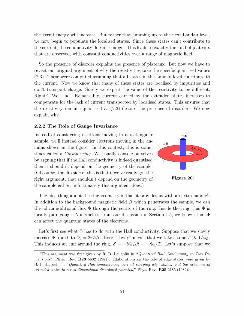
the Fermi energy will increase. But rather than jumping up to the next Landau level,
we now begin to populate the localised states. Since these states can’t contribute to
the current, the conductivity doesn’t change. This leads to exactly the kind of plateaux
that are observed, with constant conductivities over a range of magnetic field.
So the presence of disorder explains the presence of plateaux. But now we have to
revisit our original argument of why the resistivities take the specific quantised values
(2.3). These were computed assuming that all states in the Landau level contribute to
the current. Now we know that many of these states are localised by impurities and
don’t transport charge. Surely we expect the value of the resistivity to be different.
Right? Well, no. Remarkably, current carried by the extended states increases to
compensate for the lack of current transported by localised states. This ensures that
the resistivity remains quantised as (2.3) despite the presence of disorder. We now
explain why.
2.2.2 The Role of Gauge Invariance
Instead of considering electrons moving in a rectangular Φ
B
r
φ
Figure 20:
sample, we’ll instead consider electrons moving in the an-
nulus shown in the figure. In this context, this is some-
times called a Corbino ring. We usually console ourselves
by arguing that if the Hall conductivity is indeed quantised
then it shouldn’t depend on the geometry of the sample.
(Of course, the flip side of this is that if we’ve really got the
right argument, that shouldn’t depend on the geometry of
the sample either; unfortunately this argument does.)
The nice thing about the ring geometry is that it provides us with an extra handle8.
In addition to the background magnetic field B which penetrates the sample, we can
thread an additional flux Φ through the centre of the ring. Inside the ring, this Φ is
locally pure gauge. Nonetheless, from our discussion in Section 1.5, we known that Φ
can affect the quantum states of the electrons.
Let’s first see what Φ has to do with the Hall conductivity. Suppose that we slowly
increase Φ from 0 to Φ0 = 2π~/e. Here “slowly” means that we take a time T ≫ 1/ωB.
This induces an emf around the ring, E = −∂Φ/∂t = −Φ0/T . Let’s suppose that we
8This argument was first given by R. B. Laughlin in “Quantized Hall Conductivity in Two Di-
mensions”, Phys. Rev, B23 5632 (1981). Elaborations on the role of edge states were given by
B. I. Halperin in “Quantized Hall conductance, current carrying edge states, and the existence of
extended states in a two-dimensional disordered potential,” Phys. Rev. B25 2185 (1982).
– 51 –
can argue that n electrons are transferred from the inner circle to the outer circle in
this time. This would result in a radial current Ir = −ne/T .
ρxy =EIr
=2π~
e21
n(2.7)
This is the result we want. Our task, therefore, is to argue that n electrons are indeed
transferred across the ring as the flux is increased to Φ0.
Spectral Flow in Landau Levels
The key idea that we need is that of spectral flow, introduced in Section 1.5.3. The
spectrum of the Hamiltonian is the same whenever Φ is an integer multiple of Φ0.
However, if we start with a particular energy eigenstate when Φ = 0, this will evolve
into a different energy eigenstate with Φ = Φ0. As the change is done suitably slowly,
over a time T ≫ 1/ωB, the adiabatic theorem ensures that the final energy eigenstate
must lie in the same Landau level as the initial state.
To illustrate this, let’s first look at the situation with no disorder. For the ring
geometry, it is sensible to use symmetric gauge and radial coordinates, z = x−iy = reiφ.
The wavefunctions in the lowest Landau level are (1.30),
ψm ∼ zme−|z|2/4l2B = eimφrme−r2/4l2B
The mth wavefunction is strongly peaked at a radius r ≈√
2ml2B (where, of course, we
must now chose m ∈ Z such that the wavefunction lies inside the annulus). From the
discussion in Section 1.5.3, we see that if we increase the flux from Φ = 0 to Φ = Φ0,
the wavefunctions shift from m to m+ 1,
ψm(Φ = 0) −→ ψm(Φ = Φ0) = ψm+1(Φ = 0)
This means that each state moves outwards, from radius r =√
2ml2B to r =√
2(m+ 1)l2B.
The net result is that, if all states in the Landau level are filled, a single electron is
transferred from the inner ring to the outer ring as the flux is increased from Φ = 0 to
Φ = Φ0. It is simple to check that the same result holds for higher Landau levels. If
n Landau levels are filled, then n electrons are transferred from the inner to the outer
ring and the Hall resistivity is given by (2.7) as required.
Spectral Flow in the Presence of Disorder
The discussion above merely reproduces what we already know. Let’s now see how it
changes in the presence of disorder. In polar coordinates, the Hamiltonian takes the
– 52 –

form
HΦ=0 =1
2m
[
−~21
r
∂
∂r
(
r∂
∂r
)
+
(
−i~r
∂
∂φ+eBr
2
)2]
+ V (r, φ)
where V (r, φ) is the random potential capturing the effects of disorder. Note that this
depends on φ, so angular momentum is no longer a good quantum number in this
system. Adding the flux through the centre changes the Hamiltonian to
HΦ =1
2m
[
−~2 1
r
∂
∂r
(
r∂
∂r
)
+
(
−i~r
∂
∂φ+eBr
2+
eΦ
2πr
)2]
+ V (r, φ)
Importantly, the flux Φ affects only the extended states. It does not change the localised
states. To see this, we attempt to undo the flux by a gauge transformation,
ψ(r, φ) → e−ieΦφ/2π~ψ(r, φ)
For the localised states, where ψ is non-zero only in some finite region, there’s no
problem in doing this. However for the extended states, which wrap around the annulus,
we also have the requirement that the wavefunction ψ is single-valued as φ → φ+ 2π.
We see that this is only true when Φ is an integer multiple of Φ0 = 2π~/e.
The upshot of this argument is that the spectrum of the Hamiltonian is again left
unchanged when Φ is an integer multiple of Φ0. But, this time, as the flux is increased
from 0 to Φ0, the localised states don’t change. Only the extended states undergo
spectral flow; these alone must map onto themselves.
There are always at least two extended states: one near the inner ring and one near
the outer ring. The spectral flow happens in the same heuristic manner as described
above: an extended state localised at one radius is transformed into an extended state
at the next available radius. The presence of disorder means that there are fewer
extended states, but this doesn’t change the overall conclusion: if all extended states
in a given Landau level are filled, then the net effect of dialling the flux from Φ = 0
to Φ = Φ0 is to transport one electron from the inner to the outer edge. If n Landau
levels are filled, we again get the result (2.7).
The arguments above involving gauge transformations start to give a hint of the
topological nature of the quantum Hall effect. In fact, there are much deeper topological
ideas underlying the quantisation of the Hall conductivity. We’ll describe these in
Section 2.2.4 and, in a slightly different context, in Section 2.3. However, before we
proceed we first need a basic result which gives an expression for the conductivity in
any quantum mechanical system.
– 53 –

2.2.3 An Aside: The Kubo Formula
Before we get to anything related to topology, we first need to lay some groundwork.
Our task in this section will be to derive a formula for the Hall conductivity σxy in
terms of quantum mechanical observables. The expression that we’re looking for is
called the Kubo formula; it is part of more general story that goes by the name of
linear response9.
We’ll derive the Kubo formula for a general, multi-particle Hamiltonian H0 where
the subscript 0 means that this is the unperturbed Hamiltonian before we turn on an
electric field. At this point, H0 could be that of many non-interacting particles each,
for example, obeying the single-particle Hamiltonian (1.13) that we saw previously, or
it could be something more complicated. Later, we’ll apply the Kubo formula both to
Hamiltonians which describe particles moving in the continuum and to Hamiltonians
that describe particles moving on a lattice. We denote the energy eigenstates of H0 as
|m〉, with H0|m〉 = Em|m〉.
Now we add a background electric field. We work in the gauge with At = 0 so that
the electric field can be written as E = −∂tA. The new Hamiltonian takes the form
H = H0 +∆H with
∆H = −J ·A (2.8)
where J is the quantum operator associated to the electric current. For the simple
Hamiltonians that we considered in Section 1.4, J is equal (up to constants) to the me-
chanical momentum π = p+ eA = mx which we defined in equation (1.14). However,
we’ll use more general definitions of J in what follows.
At this point, there’s a couple of tricks that makes life simpler. First, we’re ultimately
interested in applying a constant, DC electric field. However, it turns out to be simpler
to apply an AC electric field, E(t) = Ee−iωt with frequency ω, and to then take the
limit ω → 0. Second, it’s also somewhat simpler if we work with a complexified A.
There’s nothing deep in this: it’s just easier to write e−iωt than, say, cos(ωt). Because
all our calculations will be to linear order only, you can take the real part at any time.
We then have
A =E
iωe−iωt (2.9)
9You can read about this story in the lecture notes on Kinetic Theory where a slightly more
sophisticated discussion of the Kubo formula can be found in Sections 4.3 and 4.4. In particular, there
is often an extra term proportional to A2 in ∆H which contributes to σxx but not σxy so is ignored
in the present discussion.
– 54 –

Our goal is to compute the current 〈J〉 that flows due to the perturbation ∆H . We will
assume that the electric field is small and proceed using standard perturbation theory.
We work in the interaction picture. This means that operators evolve as O(t) =
V −1OV with V = e−iH0t/~. In particular J, and hence ∆H(t) itself, both vary in time
in this way. Meanwhile states |ψ(t)〉, evolve by
|ψ(t)〉I = U(t, t0)|ψ(t0)〉I
where the unitary operator U(t, t0) is defined as
U(t, t0) = T exp
(
− i
~
∫ t
t0
∆H(t′) dt′)
(2.10)
Here T stands for time ordering; it ensures that U obeys the equation i~ dU/dt = ∆H U .
We’re interested in systems with lots of particles. Later we’ll only consider non-
interacting particles but, importantly, the Kubo formula is more general than this. We
prepare the system at time t→ −∞ in a specific many-body state |0〉. This is usuallytaken to be the many-body ground state, although it needn’t necessarily be. Then,
writing U(t) = U(t, t0 → −∞), the expectation value of the current is given by
〈J(t)〉 = 〈0(t)| J(t)|0(t) 〉= 〈0|U−1(t)J(t)U(t) |0〉
≈ 〈0|(
J(t) +i
~
∫ t
−∞
dt′ [∆H(t′),J(t)]
)
|0〉
where, in the final line, we’ve expanded the unitary operator (2.10), keeping only the
leading terms. The first term is the current in the absence of an electric field. We’ll
assume that this term vanishes. Using the expressions (2.8) and (2.9), the current due
to the electric field is then
〈Ji(t)〉 =1
~ω
∫ t
−∞
dt′ 〈0|[Jj(t′), Ji(t)]|0〉Ej e−iωt′
Because the system is invariant under time translations, the correlation function above
can only depend on t′′ = t− t′. We can then rewrite the expression above as
〈Ji(t)〉 =1
~ω
(∫ ∞
0
dt′′ eiωt′′ 〈0|[Jj(0), Ji(t′′)]|0〉
)
Eje−iωt
The only t dependence in the formula above sits outside as e−iωt. This is telling us that
if you apply an electric field at frequency ω, the current responds by oscillating at the
– 55 –

same frequency ω. This is the essence of linear response. The proportionality constant
defines the frequency-dependent conductivity matrix σ(ω). The Hall conductivity is
the off-diagonal part
σxy(ω) =1
~ω
∫ ∞
0
dt eiωt 〈0|[Jy(0), Jx(t)]|0〉
This is the Kubo formula for the Hall conductivity.
We can massage the Kubo formula into a slightly more useful form. We use the fact
that the current operator evolves as J(t) = V −1 J(0) V with V = e−iH0t/~. We then
evaluate σxy(ω) by inserting complete basis of energy eigenstates of H0,
σxy(ω) =1
~ω
∫ ∞
0
dt eiωt∑
n
[
〈0|Jy|n〉〈n|Jx|0〉ei(En−E0)t/~ − 〈0|Jx|n〉〈n|Jy|0〉ei(E0−En)t/~]
We now perform the integral over∫
dt. (There’s a subtlety here: to ensure convergence,
we should replace ω → ω+ iǫ, with ǫ infinitesimal. There is a story related to causality
and where poles can appear in the complex ω plane which you can learn more about
in the Kinetic Theory lecture notes.) Since the states with |n〉 = |0〉 don’t contributeto the sum, we get
σxy(ω) = − i
ω
∑
n 6=0
[〈0|Jy|n〉〈n|Jx|0〉~ω + En −E0
− 〈0|Jx|n〉〈n|Jy|0〉~ω + E0 −En
]
(2.11)
Now, finally, we can look at the DC ω → 0 limit that we’re interested in. We expand
the denominators as
1
~ω + En − E0
≈ 1
En − E0
− ~ω
(En −E0)2+O(ω2) . . .
and similar for the other term. The first term looks divergent. Indeed, such divergences
do arise for longitudinal conductivities and tell us something physical, often that mo-
mentum is conserved due to translational invariance so there can be no DC resistivity.
However, in the present case of the Hall conductivity, there is no divergence because
this term vanishes. This can be shown on general grounds from gauge invariance or,
equivalently, from the conservation of the current. Alternatively – although somewhat
weaker – it can quickly seen by rotational invariance which ensures that the expression
should be invariant under x → y and y → −x. We’re then left only with a finite
contribution in the limit ω → 0 given by
σxy = i~∑
n 6=0
〈0|Jy|n〉〈n|Jx|0〉 − 〈0|Jx|n〉〈n|Jy|0〉(En − E0)2
(2.12)
This is the Kubo formula for Hall conductivity.
– 56 –

Before we proceed, I should quickly apologise for being sloppy: the operator that we
called J in (2.8) is actually the current rather than the current density. This means
that the right-hand-side of (2.12) should, strictly speaking, be multiplied by the spatial
area of the sample. It was simpler to omit this in the above derivation to avoid clutter.
2.2.4 The Role of Topology
In this section, we describe a set-up in which we can see the deep connections between
topology and the Hall conductivity. The set-up is closely related to the gauge-invariance
argument that we saw in Section 2.2.2. However, we will consider the Hall system on
a spatial torus T2. This can be viewed as a rectangle with opposite edges identified.
We’ll take the lengths of the sides to be Lx and Ly.
We thread a uniform magnetic field B through the torus. The first result we need is
that B obeys the Dirac quantisation condition,
BLxLy =2π~
en n ∈ Z (2.13)
This quantisation arises for the same reason that we saw in Section 1.5.2 when discussing
the Berry phase. However, it’s an important result so here we give an alternative
derivation.
We consider wavefunctions over the torus and ask: what periodicity requirements
should we put on the wavefunction? The first guess is that we should insist that
wavefunctions obey ψ(x, y) = ψ(x+Lx, y) = ψ(x, y+Ly). But this turns out to be too
restrictive when there is a magnetic flux through the torus. Instead, one has to work in
patches; on the overlap between two different patches, wavefunctions must be related
by a gauge transformation.
Operationally, there is a slightly simpler way to implement this. We introduce the
magnetic translation operators,
T (d) = e−id·p/~ = e−id·(i∇+eA/~)
These operators translate a state ψ(x, y) by position vector d. The appropriate bound-
ary conditions will be that when a state is translated around a cycle of the torus, it
comes back to itself. So Txψ(x, y) = ψ(x, y) and Tyψ(x, y) = ψ(x, y) where Tx = T (d =
(Lx, 0)) and Ty = T (d = (0, Ly)).
– 57 –

It is clear from the expression above that the translation operators are not gauge
invariant: they depend on our choice of A. We’ll choose Landau gauge Ax = 0 and
Ay = Bx. With this choice, translations in the x direction are the same as those in
the absence of a magnetic field, while translations in the y direction pick up an extra
phase. If we take a state ψ(x, y), translated around a cycle of the torus, it becomes
Txψ(x, y) = ψ(x+ Lx, y) = ψ(x, y)
Tyψ(x, y) = e−ieBLyx/~ ψ(x, y + Ly) = ψ(x, y)
Notice that we can see explicitly in the last of these equations that the wavefunction
is not periodic in the naive sense in the y direction: ψ(x, y + Ly) 6= ψ(x, y). Instead,
the two wavefunctions agree only up to a gauge transformation.
However, these equations are not consistent for any choice of B. This follows by
comparing what happens if we translate around the x-cycle, followed by the y-cycle, or
if we do these in the opposite order. We have
TyTx = e−ieBLxLy/~ TxTy (2.14)
Since both are required to give us back the same state, we must have
eBLxLy~
∈ 2πZ
This is the Dirac quantisation condition (2.13).
There is an interesting story about solving for the wavefunctions of a free particle
on a torus in the presence of a magnetic field. They are given by theta functions. We
won’t discuss these here.
Adding Flux
Now we’re going to perturb the system. We do this by threading two fluxes, Φx and
Φy through the x and y-cycles of the torus respectively. This means that the gauge
potential becomes
Ax =ΦxLx
and Ay =ΦyLy
+Bx
This is the same kind of set-up that we discussed in Section 2.2.2; the only difference
is that now the geometry allows us to introduce two fluxes instead of one. Just as
in our previous discussion, the states of the quantum system are only sensitive to the
non-integer part of Φi/Φ0 where Φ0 = 2π~/e is the quantum of flux. In particular, if
we increase either Φi from zero to Φ0, then the spectrum of the quantum system must
be invariant. However, just as in Section 2.2.2, the system can undergo spectral flow.
– 58 –

The addition of the fluxes adds an extra term Φx
Φy
Figure 21:
to the Hamiltonian of the form (2.8),
∆H = −∑
i=x,y
JiΦiLi
We want to see how this affects the ground state of the
system which we will denote as |ψ0〉. (We called this
|0〉 when deriving the Kubo formula, but we’ll want to
differentiate it soon and the expression ∂0∂Φ
just looks
too odd!). We’ll assume that the ground state is non-
degenerate and that there is a gap to the first excited
state. Then, to first order in perturbation theory, the ground state becomes
|ψ0〉′ = |ψ0〉+∑
n 6=ψ0
〈n|∆H|ψ0〉En − E0
|n〉
Considering infinitesimal changes of Φi, we can write this as
|∂ψ0
∂Φi〉 = − 1
Li
∑
n 6=ψ0
〈n|Ji|ψ0〉En −E0
|n〉
But the right-hand-side is exactly the kind of expression that appeared in the Kubo
formula (2.12). This means that, including the correct factors of the spatial area, we
can write the Hall conductivity as
σxy = i~LxLy∑
n 6=ψ0
〈ψ0|Jy|n〉〈n|Jx|ψ0〉 − 〈ψ0|Jx|n〉〈n|Jy|ψ0〉(En − E0)2
= i~
[
〈∂ψ0
∂Φy| ∂ψ0
∂Φx〉 − 〈 ∂ψ0
∂Φx|∂ψ0
∂Φy〉]
= i~
[
∂
∂Φy〈ψ0|
∂ψ0
∂Φx〉 − ∂
∂Φx〈ψ0|
∂ψ0
∂Φy〉]
As we now explain, this final way of writing the Hall conductivity provides a novel
perspective on the integer quantum Hall effect.
Hall Conductivity and the Chern Number
The fluxes Φi appear as parameters in the perturbed Hamiltonian. As we discussed
above, the spectrum of the Hamiltonian only depends on Φi mod Φ0, which means that
these parameters should be thought of as periodic: the space of the flux parameters
– 59 –

is itself a torus, T2Φ, where the subscript is there to distinguish it from the spatial
torus that we started with. We’ll introduce dimensionless angular variables, θi to
parameterise this torus,
θi =2πΦiΦ0
with θi ∈ [0, 2π)
As we discussed in Section 1.5, given a parameter space it is natural to consider the
Berry phase that arises as the parameters are varied. This is described by the Berry
connection which, in this case, lives over T2Φ. It is
Ai(Φ) = −i〈ψ0|∂
∂θi|ψ0〉
The field strength, or curvature, associated to the Berry connection is given by
Fxy =∂Ax
∂θy− ∂Ay
∂θx= −i
[
∂
∂θy〈ψ0|
∂ψ0
∂θx〉 − ∂
∂θx〈ψ0|
∂ψ0
∂θy〉]
This is precisely our expression for the Hall conductivity! We learn that, for the torus
with fluxes, we can write
σxy = −e2
~Fxy
This is a nice formula. But, so far, it doesn’t explain why σxy is quantised. However,
suppose that we average over all fluxes. In this case we integrate over the torus T2Φ of
parameters to get
σxy = −e2
~
∫
T2Φ
d2θ
(2π)2Fxy
The integral of the curvature over T2Φ, is a number known as the first Chern number
C =1
2π
∫
T2Φ
d2θ Fxy
Importantly, this is always an integer: C ∈ Z. This follows from the same kind of
argument that we made in Section 1.5 (or, alternatively, the kind of argument that we
made at the beginning of this section on Dirac quantisation). The net result is that if
we average over the fluxes, the Hall conductivity is necessarily quantised as
σxy = − e2
2π~C (2.15)
This, of course, is the integer quantum Hall effect. The relationship between the Hall
conductivity and the Chern number is usually referred to as the TKNN invariant (after
Thouless, Kohomoto, Nightingale and den Nijs) although, strictly speaking, this name
should be reserved for a very similar expression that we’ll discuss in the next section.
– 60 –

2.3 Particles on a Lattice
We saw in the previous section that there is a deep relationship between the Hall
conductivity and a certain topological quantity called the Chern number that is related
to the Berry phase. Here we’ll continue to explore this relationship but in the slightly
different context of particles moving on a lattice. The kind of ideas that we will describe
have had a resurgence in recent years when it was realised that they are the key to
understanding the subject of topological insulators.
The advantage of looking at the particle on a lattice is that its momentum lies
on a torus T2, known as the Brillouin zone. It is this torus that will allow us to find
interesting topological features. Indeed, it will play a very similar role to the parameter
space T2Φ that we met in the previous section. We’ll learn that one can define a Berry
connection over the Brillouin zone and that the associated Chern number determines
the Hall conductivity.
2.3.1 TKNN Invariants
We’ll consider a particle moving on a rectangular lattice. The distance between lattice
sites in the x-direction is a; the distance in the y-direction is b. Recall from earlier
courses that the energy spectrum of this system form bands. Within each band, states
are labelled by lattice momentum which takes values in the Brillouin zone, parame-
terised by
−πa< kx ≤
π
aand − π
b< ky ≤
π
b(2.16)
The states with momenta at the edges of the Brillouin zone are identified. This means
that the Brillouin zone is a torus T2 as promised. The wavefunctions in a given band
can be written in Bloch form as
ψk(x) = eik·x uk(x) (2.17)
where uk(x) is usually periodic on a unit cell so that uk(x + e) = uk(x) with either
e = (a, 0) or e = (0, b).
We’re now in a position to describe the topology underlying the quantum Hall effect.
The results below are very general: they don’t rely on any specific Hamiltonian, but
rather apply to any system that satisfies a few simple criteria.
• First, we will assume that the single particle spectrum decomposes into bands,
with each band parameterised by a momentum label k which lives on a torus
T2. This is obviously true for simple lattice models. As we explain in Section
– 61 –

2.3.3, it is also true (under certain assumptions) for particles moving in a lattice
in the presence of a magnetic field where the torus in question is slightly different
concept called a magnetic Brillouin zone. (In this case, the periodicity conditions
on uk are altered slightly but the formula we derive below still holds.)
• Second, we’ll assume that the electrons are non-interacting. This means that we
get the multi-particle spectrum simply by filling up the single-particle spectrum,
subject to the Pauli exclusion principle.
• Finally, we’ll assume that there is a gap between bands and that the Fermi energy
EF lies in one of these gaps. This means that all bands below EF are completely
filled while all bands above EF are empty. In band theory, such a situation
describes an insulator.
Whenever these three criteria are obeyed, one can assign an integer-valued topo-
logical invariant C ∈ Z to each band. The topology arises from the way the phase of
the states winds as we move around the Brillouin zone T2. This is captured by a U(1)
Berry connection over T2, defined by
Ai(k) = −i〈uk|∂
∂ki|uk〉
There is one slight conceptual difference from the type of Berry connection we met
previously. In Section 1.5, the connections lived on the space of parameters of the
Hamiltonian; here the connection lives on the space of states itself. Nonetheless, it is
simple to see that many of the basic properties that we met in Section 1.5 still hold.
In particular, a change of phase of the states |uk〉 corresponds to a change of gauge of
the Berry connection.
We can compute the field strength associated to Ai. This is
Fxy =∂Ax
∂ky− ∂Ay
∂kx= −i
⟨
∂u
∂ky
∣
∣
∣
∣
∂u
∂kx
⟩
+ i
⟨
∂u
∂kx
∣
∣
∣
∣
∂u
∂ky
⟩
(2.18)
Once again, we can compute the first Chern number by integrating F over the Brillouin
zone T2,
C = − 1
2π
∫
T2
d2k Fxy (2.19)
In the present context, it is usually referred to as the TKNN invariant10. As we’ve seen
before, the Chern number is always an integer: C ∈ Z. In this way, we can associate
an integer Cα to each band α.10As we mentioned in the previous section, the initials stand for Thouless, Kohomoto, Nightingale
and den Nijs. The original paper is “Quantized Hall Conductance in a Two-Dimensional Periodic
Potential”, Phys. Rev. Lett. 49, 405 (1982).
– 62 –

The Chern number once again has a beautiful physical manifestation: it is related
to the Hall conductivity σxy of a non-interacting band insulator by
σxy =e2
2π~
∑
α
Cα (2.20)
where the sum is over all filled bands α and Cα is the Chern class associated to that
band. This is the famous TKNN formula. It is, of course, the same formula (2.15) that
we met previously, although the context here is rather different.
Let’s now prove the TKNN formula. Our starting point is the Kubo formula (2.12).
We previously wrote this in terms of multi-particle wavefunctions. If we’re dealing with
non-interacting particles, then these can be written as tensor products of single particle
wavefunctions, each of which is labelled by the band α and momentum k ∈ T2. The
expression for the Hall conductivity becomes
σxy = i~∑
Eα<EF<Eβ
∫
T2
d2k
(2π)2〈uαk|Jy|uβk〉〈uβk|Jx|uαk〉 − 〈uαk|Jx|uβk〉〈uβk|Jy|uαk〉
(Eβ(k)− Eα(k))2
where the index α runs over the filled bands and β runs over the unfilled bands. We
note that this notation is a little lazy; there are really separate momentum integrals for
each band and no reason that the states in the expression have the same momentum
k. Our lazy notation will save us from adding yet more annoying indices and not affect
the result below.
To make progress, we need to define what we mean by the current J. For a single, free
particle in the continuum, the current carried by the particle was simply J = ex where
the velocity operator is x = (p+ eA)/m. Here we’ll use a more general definition. We
first look at the Schrodinger equation acting on single-particle wavefunctions of Bloch
form (2.17),
H|ψk〉 = Ek|ψk〉 ⇒ (e−ik·xHeik·x)|uk〉 = Ek|uk〉⇒ H(k)|uk〉 = Ek|uk〉 with H(k) = e−ik·xHeik·x
We then define the current in terms of the group velocity of the wavepackets,
J =e
~
∂H
∂k
Before proceeding, it’s worth checking that coincides with our previous definition. In
the continuum, the Hamiltonian was simply H = (p + eA)2/2m, which gives H =
(p+ ~k+ eA)2/2m and the current due to a single particle is J = ex as expected.
– 63 –

From now on it’s merely a question of doing the algebra. The Kubo formula becomes
σxy =ie2
~
∑
Eα<EF<Eβ
∫
T2
d2k
(2π)2〈uαk|∂yH|uβk〉〈uβk|∂xH|uαk〉 − 〈uαk|∂xH|uβk〉〈uβk|∂yH|uαk〉
(Eβ(k)−Eα(k))2
where ∂x and ∂y in this expression are derivatives with respect to momenta kx and kyrespectively. We can then write
〈uαk|∂iH|uβk〉 = 〈uαk|∂i(
H|uβk〉)
− 〈uαk|H|∂iuβk〉= (Eβ(k)−Eα(k))〈uαk|∂iuβk〉= −(Eβ(k)− Eα(k))〈∂iuαk|uβk〉
The missing term, proportional to ∂iEβ , doesn’t appear because α and β are necessarily
distinct bands. Substituting this into the Kubo formula gives
σxy =ie2
~
∑
Eα<EF<Eβ
∫
T2
d2k
(2π)2〈∂yuαk|uβk〉〈uβk|∂xuαk〉 − 〈∂xuαk|uβk〉〈uβk|∂yuαk〉
But now we can think of the sum over the unfilled bands as∑
β |uβk〉〈uβk| = 1 −∑
α |uαk〉〈uαk|. The second term vanishes by symmetry, so we’re left with
σxy =ie2
~
∑
α
∫
T2
d2k
(2π)2〈∂yuαk|∂xuαk〉 − 〈∂xuαk|∂yuαk〉
where now the sum is only over the filled bands α. Comparing to (2.18), we see that
the Hall conductivity is indeed given by the sum of the Chern numbers of filled bands
as promised,
σxy = − e2
2π~
∑
α
Cα
The TKNN formula is the statement that the Hall conductivity is a topological invariant
of the system. It’s important because it goes some way to explaining the robustness of
the integer quantum Hall effect. An integer, such as the Chern number C, can’t change
continuously. This means that if we deform our system in some way then, as long as
we retain the assumptions that went into the derivation above, the Hall conductivity
can’t change: it’s pinned at the integer value.
The existence of the TKNN formula is somewhat surprising. The right-hand side
is simple and pure. In contrast, conductivities are usually thought of as something
complicated and messy, depending on all the intricate details of a system. The essence
of the TKNN formula, and indeed the quantum Hall effect itself, is that this is not the
case: the Hall conductivity is topological.
– 64 –

2.3.2 The Chern Insulator
Let’s look at an example. Perhaps surprisingly, the simplest examples of lattice models
with non-vanishing Chern numbers don’t involve any magnetic fields at all. Such lattice
models with filled bands are sometimes called Chern insulators, to highlight the fact
that they do something interesting — like give a Hall response — even though they are
insulating states.
The simplest class of Chern insulators involve just two bands. The single-particle
Hamiltonian written, written in momentum space, takes the general form
H(k) = ~E(k) · ~σ + ǫ(k)1
where k ∈ T2 and ~σ = (σ1, σ2, σ3) are the three Pauli matrices. The energies of the
two states with momentum k are ǫ(k) ± | ~E(k)|. An insulator requires a gap between
the upper and lower bands; we then fill the states of the lower band. An insulator can
only occur when ~E(k) 6= 0 for all k.
For any such model, we can introduce a unit three-vector,
~n(k) =~E(k)
| ~E(k)|
Clearly ~n describes a point on a two-dimensional sphere S2. This is the Bloch sphere.
As we move in the Brillouin zone, ~n(k) gives a map from T2 → S2 as shown in the
figure. This Chern number (2.19) for this system can be written in terms of ~n as
C =1
4π
∫
T2
d2k ~n ·(
∂~n
∂kx× ∂~n
∂ky
)
There is a particularly nice interpretation of this formula: it measures the area of the
unit sphere (counted with sign) swept out as we vary k over T2. In other words, it
counts how many times T2 wraps around S2.
Perhaps the simplest lattice model with a non-trivial Chern number arises on a square
lattice, with the Hamiltonian in momentum space given by11.
H(k) = (sin kx)σ1 + (sin ky)σ2 + (m+ cos kx + cos ky)σ3
11This model was first constructed in Xiao-Liang Qi, Yong-Shi Wu and Shou-Cheng Zhang, “Topo-
logical quantization of the spin Hall effect in two-dimensional paramagnetic semiconductors”, cond-
mat/0505308. An earlier model of a quantum Hall effect without a magnetic field, involving a honey-
comb lattice, was described by Duncan Haldane, “Model for a Quantum Hall Effect without Landau
Levels: Condensed Matter Realisation of the Parity Anomaly”, Phys. Rev. Lett. 61, 2015 (1988).
– 65 –

kx
ky
Brillouin zone
n
Bloch sphere
Figure 22: The map from Brillouin zone to Bloch sphere
In the continuum limit, this becomes the Hamiltonian for a 2-component Dirac fermion
in d = 2+1 dimensions. For this reason, this model is sometimes referred to as a Dirac-
Chern insulator.
For general values of m, the system is an insulator with a gap between the bands.
There are three exceptions: the gap closes and the two bands touch at m = 0 and
at m = ±2. As m varies, the Chern number — and hence the Hall conductivity —
remains constant as long as the gap doesn’t close. A direct computation gives
C =
−1 −2 < m < 0
1 0 < m < 2
0 |m| > 2
2.3.3 Particles on a Lattice in a Magnetic Field
So far, we’ve discussed the integer quantum Hall effect in lattice models but, perhaps
surprisingly, we haven’t explicitly introduced magnetic fields. In this section, we de-
scribe what happens when particles hop on a lattice in the presence of a magnetic field.
As we will see, the physics is remarkably rich.
To orient ourselves, first consider a particle hopping on two-dimensional square lattice
in the absence of a magnetic field. We’ll denote the distance between adjacent lattice
sites as a. We’ll work in the tight-binding approximation, which means that the position
eigenstates |x〉 are restricted to the lattice sites x = a(m,n) with m,n ∈ Z. The
Hamiltonian is given by
H = −t∑
x
∑
j=1,2
|x〉〈x+ ej|+ h.c. (2.21)
– 66 –

where e1 = (a, 0) and e2 = (0, a) are the basis vectors of the lattice and t is the hopping
parameter. (Note: t is the standard name for this parameter; it’s not to be confused
with time!) The lattice momenta k lie in the Brillouin zone T2, parameterised by
−πa< kx ≤
π
aand − π
a< ky ≤
π
a(2.22)
Suppose that we further make the lattice finite in spatial extent, with size L1×L2. The
momenta ki are now quantised in units of 1/2πLi. The total number of states in the
Brillouin zone is then (2πa/ 12πL1
)× (2πa/ 12πL1
) = L1L2/a2. This is the number of sites in
the lattice which is indeed the expected number of states in the Hilbert space.
Let’s now add a background magnetic field to the story. The first thing we need to
do is alter the Hamiltonian. The way to do this is to introduce a gauge field Aj(x)
which lives on the links between the lattice sites. We take A1(x) to be the gauge field
on the link to the right of point x, and A2(x) to be the gauge field on the link above
point x, as shown in the figure. The Hamiltonian is then given by
H = −t∑
x
∑
j=1,2
|x〉e−ieaAj(x)/~〈x+ ej |+ h.c. (2.23)
It might not be obvious that this is the correct way to
A (x)1
A (x+e )
x
1
A (x)2
x+e +e
2
x+e
x+e
12 2
1
1
1
A (x+e +e )2
Figure 23:
incorporate a magnetic field. To gain some intuition,
consider a particle which moves anti-clockwise around a
plaquette. To leading order in t, it will pick up a phase
e−iγ , where
γ =ea
~(A1(x) + A2(x+ e1)−A1(x+ e2)−A2(x))
≈ ea2
~
(
∂A2
∂x1− ∂A1
∂x2
)
=ea2B
~
where B is the magnetic field which passes through the
plaquette. This expression is the same as the Aharonov-Bohm phase (1.49) for a particle
moving around a flux Φ = Ba2.
Let’s now restrict to a constant magnetic field. We can again work in Landau gauge,
A1 = 0 and A2 = Bx1 (2.24)
We want to understand the spectrum of the Hamiltonian (2.23) in this case and, in
particular, what becomes of the Brillouin zone.
– 67 –

Magnetic Brillouin Zone
We saw above that the key to finding topology in a lattice system was the presence
of the Brillouin zone T2. Yet it’s not immediately obvious that the Brilliouin zone
survives in the presence of the magnetic field. The existence of lattice momenta k are
a consequence of the discrete translational invariance of the lattice. But, as usual, the
choice of gauge breaks the explicit translational invariance of the Hamiltonian, even
though we expect the underlying physics to be translational invariant.
In fact, we’ll see that the interplay between lattice effects and magnetic effects leads
to some rather surprising physics that is extraordinarily sensitive to the flux Φ = Ba2
that threads each plaquette. In particular, we can define a magnetic version of the
Brillouin zone whenever Φ is a rational multiple of Φ0 = 2π~/e,
Φ =p
qΦ0 (2.25)
with p and q integers which share no common divisor. We will see that in this situation
the spectrum splits up into q different bands. Meanwhile, if Φ/Φ0 is irrational, there
are no distinct bands in the spectrum: instead it takes the form of a Cantor set!
Nonetheless, as we vary Φ/Φ0, the spectrum changes continuously. Needless to say, all
of this is rather odd!
We start by defining the gauge invariant translation operators
Tj =∑
x
|x〉e−ieaAj(x)/~〈x+ ej |
This shifts each state by one lattice site; T1 moves us to the left and T †1 to the right,
while T2 moves us down and T †2 up, each time picking up the appropriate phase from
the gauge field. Clearly we can write the Hamiltonian as
H = −t(
∑
j=1,2
Tj + T †j
)
These translation operators do not commute. Instead it’s simple to check that they
obey the nice algebra
T2 T1 = eieΦ/~T1 T2 (2.26)
This is the discrete version of the magnetic translation algebra (2.14). In the present
context it means that [Ti, H ] 6= 0 so, in the presence of a magnetic field, we don’t get
to label states by the naive lattice momenta which would be related to eigenvalues of
Ti. This shouldn’t be too surprising: the algebra (2.26) is a reflection of the fact that
the gauge invariant momenta don’t commute in a magnetic field, as we saw in (1.15).
– 68 –

However, we can construct closely related operators that do commute with Tj and,
hence, with the Hamiltonian. These are defined by
Tj =∑
x
|x〉e−ieaAj(x)/~〈x+ ej |
where the new gauge field Aj is constructed to obey ∂kAj = ∂jAk. In Landau gauge,
this means that we should take
A1 = Bx2 and A2 = 0
When this holds, we have
[Tj , Tk] = [T †j , Tk] = 0 ⇒ [H, Tj] = 0
These operators commute with the Hamiltonian, but do not themselves commute. In-
stead, they too obey the algebra (2.26).
T2 T1 = eieΦ/~ T1 T2 (2.27)
This means that we could label states of the Hamiltonian by eigenvalues of, say, T2but not simultaneously by eigenvalues of T1. This isn’t enough to construct a Brillouin
zone.
At this point, we can see that something special happens when the flux is a rational
multiple of Φ0, as in (2.25). We can now build commuting operators by
[T n1
1 , T n2
2 ] = 0 wheneverp
qn1n2 ∈ Z
This means in particular that we can label energy eigenstates by their eigenvalue under
T2 and, simultaneously, their eigenvalue under T q1 . We call these states |k〉 with k =
(k1, k2). They are Bloch-like eigenstates, satisfying
H|k〉 = E(k)|k〉 with T q1 |k〉 = eiqk1a|k〉 and T2|k〉 = eik2a|k〉
Note that the momenta ki are again periodic, but now with the range
− π
qa< k1 ≤
π
qaand − π
a< k2 ≤
π
a(2.28)
The momenta ki parameterise the magnetic Brillouin zone. It is again a torus T2, but
q times smaller than the original Brillouin zone (2.22). Correspondingly, if the lattice
has size L1 × L2, the number of states in each magnetic Brillouin zone is L1L2/qa2.
This suggests that the spectrum decomposes into q bands, each with a different range
of energies. For generic values of p and q, this is correct.
– 69 –

The algebraic structure above also tells us that any energy eigenvalue in a given band
is q-fold degenerate. To see this, consider the state T1|k〉. Since [H, T1] = 0, we know
that this state has the same energy as |k〉: HT1|k〉 = E(k)T1|k〉. But, using (2.27),
the ky eigenvalue of this state is
T2(T1|k〉) = eieΦ/~T1T2|k〉 = ei(2πp/q+k2a)T1|k〉
We learn that |k〉 has the same energy as T1|k〉 ∼ |(k1, k2 + 2πp/qa)〉.
The existence of a Brillouin zone (2.28) is the main result we need to discuss Hall
conductivities in this model. However, given that we’ve come so far it seems silly not
to carry on and describe what the spectrum of the Hamiltonian (2.23) looks like. Be
warned, however, that the following subsection is a slight detour from our main goal.
Hofstadter Butterfly
To further understand the spectrum of the Hamiltonian (2.23), we’ll have to roll up
our sleeves and work directly with the Schrodinger equation. Let’s first look in position
space. We can write the most general wavefunction as a linear combination of the
position eigenstates |x〉,
|ψ〉 =∑
x
ψ(x)|x〉
The Schrodinger equation H|ψ〉 = E|ψ〉 then becomes an infinite system of coupled,
discrete equations
[
ψ(x+ e1) + ψ(x− e1) + e−i2πpx1/qaψ(x+ e2) + e+i2πpx
1/qaψ(x− e2)]
= −Etψ(x)
We want to find the possible energy eigenvalues E.
The way we usually solve these kinds of problems is by doing a Fourier transform of
the wavefunction to work in momentum space, with
ψ(k) =∑
x
e−ik·x ψ(x) (2.29)
where, since x takes values on a discrete lattice, k takes values in the original Brillouin
zone (2.22). In the absence of a magnetic field, modes with different momenta k
decouple from each other. However, if you try the same thing in the presence of a
magnetic field, you’ll find that the modes with momentum k = (k1, k2) couple to
modes with momentum (k1 + 2πp/qa, k2). The reflects the fact that, as we have seen,
– 70 –

the magnetic Brillouin zone (2.28) is q times smaller. For this reason, we instead split
the wavefunction (2.29) into q different wavefunctions ψr(k), with r = 1, . . . , q as
ψr(k) =∑
x
e−i(k1+2πpr/qa,k2)·x ψ(x)
These contain the same information as (2.29), but now the argument k ranges over the
magnetic Brillouin zone (2.28). Given the wavefunctions ψr, we can always reconstruct
ψ(x) by the inverse Fourier transform,
ψ(x) =
q∑
r=1
∫ +π/qa
−π/qa
dk12π
∫ +π/a
−π/a
dk22π
eik·x ψr(k)
In this way, we see that we have a q-component vector of wavefunctions, ψr(k) living
on the magnetic Brillouin zone.
Taking the Fourier transform of the discrete Schrodinger equation in position space
yields the following equation
2 cos
(
k1a+2πpr
q
)
ψr(k) + eik2aψr+1(k) + e−ik2aψr−1(k) = −E(k)t
ψr(k)
This is known as the Harper equation.
The Harper equation can be solved numerically. The resulting spectrum is quite
wonderful. For rational values, Φ/Φ0 = p/q, the spectrum indeed decomposes into
q bands with gaps between them, as we anticipated above. Yet the spectrum also
varies smoothly as we change Φ. Obviously if we change Φ/Φ0 continuously it will
pass through irrational values; when this happens the spectrum forms something like a
Cantor set. The result is a beautiful fractal structure called the Hofstadter butterfly12
shown in Figure 24. Here, a point is drawn in black if there is a state with that energy.
Otherwise it is white. To get a sense of the structure, you could look at the specific
values Φ/Φ0 = 1/q, above which you should see q vertical bands of black.
TKNN Invariants for Particles on a Lattice in a Magnetic Field
Finally we reach our main goal: to compute the Hall conductivity of the lattice model
for a particle in a background magnetic field. We can only do this for rational fluxes
12The spectrum was first solved numerically by Douglas Hofstadter in ”Energy levels and
wave functions of Bloch electrons in rational and irrational magnetic fields”, Phys. Rev.
B14, 2239 (1976). The picture of the butterfly was taken from Or Cohen’s webpage
http://phelafel.technion.ac.il/∼orcohen/butterfly.html where you can find a nice description of the
techniques used to generate it.
– 71 –

Figure 24: The Hofstadter butterfly
Φ = pΦ0/q for which there exists a magnetic Brillouin zone. In this case, we can
use the TKNN formula (2.20), but with the Chern number, which used to be defined
by integrating over the Brillouin zone, now arising by integrating over the magnetic
Brillouin zone.
The computation of the Chern numbers is not so straightforward. (You can find it
in the original paper of TKNN or, in more detail, in the book by Fradkin). Here we
just state the answer. Even this is not totally straightforward.
First consider the rth of the q bands. Then, to compute the Chern number, you are
invited to solve the linear Diophantine equation
r = qsr + ptr
with |tr| ≤ q/2. The Chern number of the rth band is given by
Cr = tr − tr−1
where t0 ≡ 0. If the first r bands are filled, so that Er < EF < Er+1, then the Hall
conductivity is given by
σxy =e2
2π~tr
It’s helpful to look at some examples. First, when Φ = pΦ0, there is only a single
band and the Hall conductivity vanishes. A more complicated, illustrative example
– 72 –

is given by p/q = 11/7. Here the solutions to the Diophantine equation are (sr, tr) =
(−3, 2), (5,−3), (2,−1), (−1, 1), (−4, 3), (4,−2), (1, 0). As we fill consecutive bands, the
second number tr in these pairs determines the Hall conductivity. We see that the Hall
conductivity varies in an interesting way, sometimes negative and sometimes positive.
– 73 –

3. The Fractional Quantum Hall Effect
We’ve come to a pretty good understanding of the integer quantum Hall effect and
the reasons behind it’s robustness. Indeed, some of the topological arguments in the
previous chapter are so compelling that you might think the Hall resistivity of an
insulator has to be an integer. But each of these arguments has a subtle loophole and
ultimately they hold only for non-interacting electrons. As we will now see, much more
interesting things can happen when we include interactions.
As with the integer quantum Hall effect, these interesting things were first discovered
by experimenters rather than theorists. Indeed, it came as a great surprise to the
community when, in 1982, plateaux in the Hall resistivity were seen at non-integer
filling fractions. These plateaux were first seen at filling fraction ν = 13and 2
3, and
later at ν = 15, 25, 37, 49, 59, 35, . . . in the lowest Landau level and ν = 4
3, 53, 75, 52, 12
5, 13
5, . . .
in higher Landau levels, as well as many others. There are now around 80 quantum
Hall plateaux that have been observed. A number of these are shown below13:
There’s two things that we can say immediately. First, the interactions between elec-
trons must be playing some role. And second, the answer to why these plateaux form
is likely to be very hard. Let’s see why.
Suppose, for the sake of argument, that we have ν < 1 so that the lowest Landau
level is partially filled. Each Landau level can house N = AB/Φ0 (spin polarised)
13This data is from R. Willett, J. P. Eisenstein, H. L. Stormer, D. C. Tsui, A. C. Gossard and
H. English “Observation of an Even-Denominator Quantum Number in the Fractional Quantum Hall
Effect”, Phys. Rev. Lett. 59, 15 (1987).
– 74 –

E E
Figure 25: Density of states in the lowest
Landau level without interactions
Figure 26: ...and with interactions (with
only a single gap at ν = 1/3 shown.
electrons, where B is the magnetic field and A is the area of the sample. This is a
macroscopic number of electrons. The number of ways to fill νN of these states is(
NνN
)
which, using Stirling’s formula, is approximately(
1ν
)νN ( 11−ν
)(1−ν)N. This is a
ridiculously large number: an exponential of an exponential. The ground state of any
partially filled Landau level is wildly, macroscopically degenerate.
Now consider the effect of the Coulomb interaction between electrons,
VCoulomb =e2
4πǫ0|ri − rj|(3.1)
On general grounds, we would expect that such an interaction would lift the degen-
eracy of ground states. But how to pick the right one? The approach we’re taught
as undergraduates is to use perturbation theory. But, in this case, we’re stuck with
extraordinarily degenerate perturbation theory where we need to diagonalise a macro-
scopically large matrix. That’s very very hard. Even numerically, no one can do this
for more than a dozen or so particles.
We can, however, use the experiments to intuit what must be going on. As we
mentioned above, we expect the electron interactions to lift the degeneracy of the
Landau level, resulting in a spectrum of states of width ∼ ECoulomb. The data would
be nicely explained if this spectrum had gaps at the filling fractions ν where Hall states
are seen. In the picture above, we’ve depicted just a single gap at ν = 1/3. Presumably
though there are many gaps at different fractions: the more prominent the plateaux,
the larger the gap.
Then we can just re-run the story we saw before: we include some disorder, which
introduces localised states within the gap, which then gives rise both to the plateaux
– 75 –
in ρxy and the observed ρxx = 0. The bigger the gap, the more prominent the observed
plateaux. This whole story requires the hierarchy of energy scales,
~ωB ≫ ECoulomb ≫ Vdisorder
We will assume in what follows that this is the case. The question that we will focus
on instead is: what is the physics of these fractional quantum Hall states?
In what follows, we will take advantage of the difficulty of a direct theoretical attack
on the problem to give us license to be more creative. As we’ll see, the level of rigour
in the thinking about the fractional quantum Hall effect is somewhat lower than that
of the integer effect. Instead, we will paint a compelling picture, using a number of
different approaches, to describe what’s going on.
3.1 Laughlin States
The first approach to the fractional quantum Hall effect was due to Laughlin14, who
described the physics at filling fractions
ν =1
m
with m an odd integer. As we’ve explained above, it’s too difficult to diagonalise the
Hamiltonian exactly. Instead Laughlin did something very bold: he simply wrote down
the answer. This was motivated by a combination of physical insight and guesswork.
As we will see, his guess isn’t exactly right but, it’s very close to being right. More
importantly, it captures all the relevant physics.
3.1.1 The Laughlin Wavefunction
Laughlin’s wavefunction didn’t come out of nowhere. To motivate it, let’s start by
considering an illuminating toy model.
Two Particles
Consider two particles interacting in the lowest Landau level. We take an arbitrary
central potential between them,
V = V (|r1 − r2|)
Recall that in our first courses on classical mechanics we solve problems like this by
using the conservation of angular momentum. In quantum physics, this means that we
14The original paper is “Anomalous quantum Hall effect: An Incompressible quantum fluid with
fractionally charged excitations” , Phys. Rev. Lett. 50 (1983) 1395.
– 76 –

work with eigenstates of angular momentum. As we saw in Section 1.4, if we want to
talk about angular momentum in Landau levels, we should work in symmetric gauge.
The single particle wavefunctions in the lowest Landau level take the form (1.30)
ψm ∼ zme−|z|2/4l2B
with z = x − iy. These states are localised on a ring of radius r =√2mlB. The
exponent m of these wavefunctions labels the angular momentum. This can be seen by
acting with the angular momentum operator (1.31),
J = i~
(
x∂
∂y− y
∂
∂x
)
= ~(z∂ − z∂) ⇒ Jψm = ~mψm
Rather remarkably, this information is enough to solve our two-particle problem for
any potential V ! As long as we neglect mixing between Landau levels (which is valid
if ~ωB ≫ V ) then the two-particle eigenstates for any potential must take the form
ψ ∼ (z1 + z2)M(z1 − z2)
me−(|z1|2+|z2|2)/4l2B
where M,m are non-negative integers, with M determining the angular momentum of
the centre of mass, and m the relative angular momentum. Note that here, and below,
we’ve made no attempt to normalise the wavefunctions.
It’s surprising that we can just write down eigenfunctions for a complicated potential
V (r) without having to solve the Schrodinger equation. It’s even more surprising that
all potentials V (r) have the same energy eigenstates. It is our insistence that we lie in
the lowest Landau level that allows us to do this.
Many-Particles
Unfortunately, it’s not possible to generalise arguments similar to those above to
uniquely determine the eigenstates for N > 2 particles. Nonetheless, on general
grounds, any lowest Landau level wavefunction must take the form,
ψ(z1, . . . , zn) = f(z1, . . . , zN)e−
∑Ni=1 |zi|
2/4l2B (3.2)
for some analytic function f(z). Moreover, this function must be anti-symmetric under
exchange of any two particle zi ↔ zj , reflecting the fact that the underlying electrons
are fermions.
– 77 –

Laughlin’s proposal for the ground state wavefunction at filling fraction ν = 1/m is:
ψ(zi) =∏
i<j
(zi − zj)me−
∑ni=1 |zi|
2/4l2B (3.3)
Clearly this is anti-symmetric when m is an odd integer. For m an even integer, it
can be thought of as a quantum Hall state for bosons. The pre-factor vanishes with
a zero of order m whenever two electrons come together. Meanwhile, the exponential
factor decreases quickly whenever the electrons get too far away from the origin. The
wavefunction is peaked on configurations that balance these two effects.
Let’s first show that the wavefunction has the desired filling fraction. To do this,
focus on what the wavefunction is telling us about a single particle, say z1. The terms
that depend on z1 in the pre-factor of the Laughlin wavefunction are
∏
i<j
(zi − zj)m ∼
N∏
i=2
(z1 − zi)m
which tells us that there are m(N − 1) powers of z1. This, in turn, tells us that the
maximum angular momentum of the first particle is m(N − 1) and so its maximum
radius is R ≈√2mNlB. Correspondingly, the area of the droplet is A ≈ 2πmNl2B
(where we’ve replaced N − 1 with N). Recall that the number of states in the full
Landau level is AB/Φ0 = A/2πl2B ≈ mN . This argument gives us the filling fraction
ν =1
m(3.4)
as promised.
It can be shown numerically that, at least for small numbers of particles, this wave-
function has greater than 99% overlap with the true ground state arising arising from
both the Coulomb repulsion (3.1) as well as a number of other repulsive potentials V .
Heuristically this occurs because the wavefunction has a zero of order m whenever two
electrons coincide. Of course, a single zero is guaranteed by Pauli exclusion, but the
Laughlin wavefunction does more. It’s as if each electron carves out a space around it
which helps it minimise the energy for repulsive potentials.
The high numerical overlap with the true ground state is often put forward as strong
evidence for the veracity of the Laughlin wavefunction. While it’s certainly impressive,
this isn’t the reason that the Laughlin wavefunction is interesting. Finding the ground
state numerically is difficult and can only be done for a couple of dozen particles. While
this may provide 99.99% overlap with the Laughlin wavefunction, by the time we get
– 78 –

to 1011 particles or so, the overlap is likely to be essentially zero. Instead, we should
think of the Laughlin wavefunctions as states which lie in the same “universality class”
as the true ground state. We will explain what this means in Section 3.2 but, roughly
speaking, it is the statement that the states have the same fractional excitations and
the same topological order as the true ground states.
The Fully Filled Landau Level
From the arguments above, the Laughlin state (3.3) with m = 1 should describe a
completely filled Landau level. But this is something we can compute in the non-
interacting picture and it provides a simple check on the Laughlin ansatz.
Let us first review how to build the many-particle wavefunction for non-interacting
electrons. Suppose that N electrons sit in states ψi(x), with 1 = 1, . . . , N . Because
the electrons are fermions, these states must be distinct. To build the many-particle
wavefunction, we need to anti-symmetrise over all particles. This is achieved by the
Slater determinant,
ψ(xi) =
∣
∣
∣
∣
∣
∣
∣
∣
∣
∣
∣
ψ1(x1) ψ1(x2) . . . ψ1(xN )
ψ2(x1) ψ2(x2) . . . ψ2(xN )...
...
ψN (x1) ψN (x2) . . . ψN (xN)
∣
∣
∣
∣
∣
∣
∣
∣
∣
∣
∣
(3.5)
We can now apply this to the lowest Landau level, with the single-particle states built
up with successive angular momentum quantum numbers
ψm(z) ∼ zm−1e−|z|2/4l2B m = 1, . . . , N
The resulting Slater determinant gives a state of the general form (3.2), with f(zi)
given by a function known as the Vandermonde determinant,
f(zi) =
∣
∣
∣
∣
∣
∣
∣
∣
∣
∣
∣
z01 z02 . . . z0N
z1 z2 . . . z3...
...
zN−11 zN−1
2 . . . zN−1N
∣
∣
∣
∣
∣
∣
∣
∣
∣
∣
∣
=∏
i<j
(zi − zj)
To see that the determinant is indeed given by the product factor, note that∏
i<j(zi−zj)is the lowest order, fully anti-symmetric polynomial (because any such polynomial must
have a factor (zi−zj) for each pair i 6= j). Meanwhile, the determinant is also completely
– 79 –

anti-symmetric and has the same order as the product factor. This ensures that they
must be equal up to an overall numerical factor which can be checked to be 1. We see
that m = 1 Laughlin state does indeed agree with the wavefunction for a completely
filled lowest Landau level.
The Competing Phase: The Wigner Crystal
The Laughlin state should be thought of as a liquid phase of electrons. In fact, strictly
speaking, it should be thought of as an entirely new phase of matter, distinguished by
a property called topological order which we’ll discuss in Section 3.2.4. But, if you’re
looking for a classical analogy, a liquid is the best.
There is a competing solid phase in which the electrons form a two-dimensional
triangular lattice, known as a Wigner crystal. Indeed, before the discovery of the
quantum Hall effect, it was thought that this would be the preferred phase of electrons
in high magnetic fields. It’s now known that the Wigner crystal has lower energy than
the Laughlin state only when the densities of electrons are low. It is observed for filling
fractions ν . 17
3.1.2 Plasma Analogy
The Laughlin wavefunctions (3.3) are very easy to write down. But it’s hard to actually
compute with them. The reason is simple: they are wavefunctions for a macroscopic
number of particles which means that if we want to compute expectation values of
operators, we’re going to have to do a macroscopic number of integrals∫
d2zi. And
that’s difficult.
For example, suppose that we want to figure out the average density of the quantum
Hall droplet. We need to compute the expectation value of the density operator
n(z) =N∑
i=1
δ(z − zi)
This is given by
〈ψ|n(z)|ψ〉 =∫∏N
i=1 d2zi n(z)P [zi]
∏Ni=1 d
2zi P [zi](3.6)
where we’ve introduced the un-normalised probability density associated to the Laugh-
lin wavefunction
P [zi] =∏
i<j
|zi − zj |2ml2mB
e−∑
i |zi|2/2l2B (3.7)
The integrals in (3.6) are hard. How to proceed?
– 80 –
The key observation is that the expectation value (3.6) has the same formal structure
as the kind of things we compute in classical statistical mechanics, with the denominator
interpreted as the partition function,
Z =N∏
i=1
d2zi P [zi]
Indeed, we can make this analogy sharper by writing the probability distribution (3.7)
so it looks like a Boltzmann distribution function,
P [zi] = e−βU(zi)
with
βU(zi) = −2m∑
i<j
log
( |zi − zj |lB
)
+1
2l2B
N∑
i=1
|zi|2
Of course, this hasn’t helped us do the integrals. But the hope is that perhaps we can
interpret the potential U(zi) as something familiar from statistical physics which will
at least provide us with some intuition for what to expect. And, indeed, this does turn
out to be the case, but only if we pick β — which, in a statistical mechanics context is
interpreted as inverse temperature — to take the specific value
β =2
m(3.8)
I stress that the quantum Hall state isn’t placed at a finite temperature. This is an
auxiliary, or fake, “temperature”. Indeed, you can tell it’s not a real temperature
because it’s dimensionless! To compensate, the potential is also dimensionless, given
by
U(zi) = −m2∑
i<j
log
( |zi − zj |lB
)
+m
4l2B
N∑
i=1
|zi|2 (3.9)
We’ll now show that this is the potential energy for a plasma of charged particles
moving in two-dimensions, where each particle carried electric charge q = −m.
The first term in (3.9) is the Coulomb potential between two particles of charge
q when both the particle and the electric field lines are restricted to lie in a two-
dimensional plane. To see this, note that Poisson equation in two dimensions tells us
that the electrostatic potential generated by a point charge q is
−∇2φ = 2πqδ2(r) ⇒ φ = −q log(
r
lB
)
The potential energy between two particles of charge q is then U = qφ, which is indeed
the first term in (3.9).
– 81 –

The second term in (3.9) describes a neutralising background of constant charge. A
constant background of charge density ρ0 would have electrostatic potential obeying
−∇2φ = 2πρ0. Meanwhile, the second term in the potential obeys
−∇2
( |z|24l2B
)
= − 1
l2B
which tells us that each electron feels a background charge density
ρ0 = − 1
2πl2B(3.10)
Note that this is equal (up to fundamental constants) to the background flux B in the
quantum Hall sample.
Now we can use our intuition about this plasma. To minimise the energy, the plasma
will want to neutralise, on average, the background charge density. Each particle carries
charge q = −m which means that the compensating density of particles n should be
mn = ρ0, or
n =1
2πl2Bm
This is the expected density of a state at filling fraction ν = 1/m. This argument has
also told us something new. Naively, the form of the Laughlin wavefunction makes it
look as if the origin is special. But that’s misleading. The plasma analogy tells us that
the average density of particles is constant.
The plasma analogy can also help answer more detailed questions about the variation
of the density (3.6) on shorter distance scales. Intuitively, we might expect that at
low temperatures (keeping the density fixed), the plasma forms a solid, crystal like
structure, while at high temperatures it is a liquid. Alternatively, at low densities
(keeping the temperature fixed) we would expect it to form a solid while, at high
densities, it would be a liquid. To determine the structure of the Laughlin wavefunction,
we should ask which phase the plasma lies in at temperature β = 2/m and density
n = 1/2πl2Bm.
This is a question which can only be answered by numerical work. It turns out that
the plasma is a solid when m & 70. For the low m of interest, in particular m = 3 and
5, the Laughlin wavefunction describes a liquid. (Note that this is not the same issue as
whether the Wigner crystal wavefunction is preferred over the Laughlin wavefunction:
it’s a question of whether the Laughlin wavefunction itself describes a liquid or solid).
– 82 –
3.1.3 Toy Hamiltonians
The Laughlin state (3.3) is not the exact ground state of the Hamiltonian with Coulomb
repulsion. However, it is possible to write down a toy Hamiltonian whose ground state
is given by the Laughlin state. Here we explain how to do this, using some tools which
will also provide us with a better understanding of the general problem.
Let’s go back to the problem of two particles interacting through a general central
potential V (|r1 − r2|). As we saw in Section 3.1.1, in the lowest Landau level the
eigenstates for any potential are the same, characterised by two non-negative integers:
the angular momentum of the centre of mass M and the relative angular momentum
m,
|M,m〉 ∼ (z1 + z2)M(z1 − z2)
me−(|z1|2+|z2|2)/4l2B
We should take m odd if the particles are fermions, m even if they are bosons.
The eigenvalues of the potential V are given by
vm =〈M,m|V |M,m〉〈M,m|M,m〉 (3.11)
These eigenvalues are sometimes referred to as Haldane pseudopotentials. For central
potentials, they do not depend on the overall angular momentum M .
These eigenvalues capture a crude picture of the spatial profile of the potential. This
is because, as we have seen, the wavefunctions |M,m〉 are peaked on a circle of radius
r ≈√2mlB. Correspondingly, the eigenvalues are roughly
vm ≈ V (r =√2mlB) (3.12)
This means that typically the vm are positive for a repulsive potential and negative for
an attractive potential, in each case falling off as V (r) as m increases.
Importantly, however, the eigenvalues are discrete. This simple fact is telling us
some interesting physics: it means that each of the states |M,m〉 can be thought of
as a bound state of two particles, even if the potential is repulsive! This is in stark
contrast to quantum mechanics in the absence of a magnetic field where there are no
discrete-energy bound states for a repulsive potential, only scattering states with a
continuous spectrum. But the magnetic field changes this behaviour.
– 83 –

Given the eigenvalues vm, we can always reconstruct the potential V . In this lowest
Landau level, there is no kinetic energy and the potential is the only contribution to
the Hamiltonian. It’s useful to write it as
H =∑
m′
vm′Pm′ (3.13)
where Pm is the operator which projects onto states in which the two particles have
relative angular momentum m.
Now we can just pick whatever vm we like to design our own Hamiltonians. Of course,
they may not be very realistic when written in terms of V (r) but we won’t let that
bother us too much. In this spirit, consider the choice
vm′ =
1 m′ < m
0 m′ ≥ m(3.14)
This Hamiltonian means that you pay an energy cost if the relative angular momentum
of the particles dips below some fixed value m. But it costs you nothing to have a high
angular momentum. In position space, the equation (3.12) tells us that there’s a finite
energy cost if the particles get too close.
Toy Hamiltonians for Many Particles
We can also use the pseudopotentials to construct Hamiltonians for N particles. To
do this, we introduce the operator Pm(ij). This projects the wavefunction onto the
state in which the ith and jth particles have relative angular momentum m. We then
construct the Hamiltonian as
H =
∞∑
m′=1
∑
i<j
vm′Pm′(ij) (3.15)
Note, however, that Pm(ij) and Pm(kj) do not commute with each other. This is what
makes these many-particle Hamiltonians difficult to solve.
Now consider the many-particle Hamiltonian with vm′ given by (3.14). This time,
you pay an energy cost whenever the relative angular momentum of any pair of particles
is less than m. You can avoid this energy cost by including a factor of (zi − zj)m for
each pair of particles, and writing down a wavefunction of the form
ψ(zi) = s(zi)∏
i<j
(zi − zj)m e−
∑i |zi|
2/4l2B (3.16)
where s(zi) can be any symmetric polynomial in the zi to preserve the statistics of the
particles. All such wavefunctions have the vanishing energy.
– 84 –
So far this doesn’t pick out the Laughlin state, which has s(zi) = 1, as the ground
state. But there is something special about this state: among all states (3.16), it is the
most compact. Indeed, we saw in Section 3.1.1 that it takes up an area A = 2πmNl2B.
Any state with s(zi) 6= 1 necessarily spreads over a larger spatial area. This means that
the Laughlin wavefunction will be the ground state if we also add a confining potential
to the system.
We can state this in a slightly different way in terms of angular momentum. We know
that states with higher angular momentum sit at larger radius. This means that we
can take the total angular momentum operator J as a proxy for the confining potential
and consider the Hamiltonian
H =
m−1∑
m′=1
∑
i<j
Pm′(ij) + ωJ (3.17)
The Laughlin wavefunction has the lowest energy: E0 =12ωmN(N−1). Any wavefunc-
tion of the form (3.16) with s(zi) 6= 1 has spatial extent larger than the ground state,
and hence higher angular momentum, and so costs extra energy due to the second
term; any wavefunction with spatial extent smaller than the Laughlin wavefunction
necessarily has a pair of particles with relative angular momentum less than m and so
pays an energy cost due to the first term.
The fact that it costs a finite energy to squeeze the wavefunction is expected to
hold for more realistic Hamiltonians as well. It is usually expressed by saying that
the quantum Hall fluid is incompressible. This is responsible for the gap in the bulk
spectrum described in the introduction of this section. However, it turns out that the
dynamics of states with s(zi) 6= 1 contains some interesting information. We’ll return
to this in Section 6.1.
3.2 Quasi-Holes and Quasi-Particles
So far, we’ve only discussed the ground state of the ν = 1/m quantum Hall systems.
Now we turn to their excitations. There are two types of charged excitations, known
as quasi-holes and quasi-particles. We discuss them in turn.
Quasi-Holes
The wavefunction describing a quasi-hole at position η ∈ C is
ψhole(z; η) =
N∏
i=1
(zi − η)∏
k<l
(zk − zl)m e−
∑ni=1 |zi|
2/4l2B (3.18)
– 85 –

We see that the electron density now vanishes at the point η. In other words, we have
created a “hole” in the electron fluid. More generally, we can introduce M quasi-holes
in the quantum Hall fluid at positions ηj with j = 1, . . . ,M , with wavefunction
ψM−hole(z; η) =
M∏
j=1
N∏
i=1
(zi − ηj)∏
k<l
(zk − zl)m e−
∑ni=1 |zi|
2/4l2B (3.19)
The quasi-hole has a remarkable property: it carries a fraction of the electric charge of
the electron! In our convention, the electron has charge −e; the quasi-hole has charge
e∗ = +e/m.
A heuristic explanation of the fractional charge follows from noting that if we place
m quasi-holes at the same point η then the wavefunction becomes
ψm−hole(z; η) =N∏
i=1
(zi − η)m∏
k<l
(zk − zl)m e−
∑ni=1 |zi|
2/4l2B
If η was a dynamical variable, as opposed to a parameter, this is just the original
wavefunction with an extra electron at position η. But because η is not a dynamical
variable, but instead a parameter, it’s really a Laughlin wavefunction that describes a
deficit of a single electron at position η. This means that m holes act like a deficit of a
single electron, so a single quasi-hole is 1/mth of an electron. It should therefore carry
charge +e/m.
We can make exactly the same argument in the context of the plasma analogy for
the quasi-hole wavefunction (3.18). The resulting plasma potential energy has an extra
term compared to (3.9),
U(zi) = −m2∑
i<j
log
( |zi − zj |lB
)
−m∑
i
log
( |zi − η|lB
)
+m
4l2B
N∑
i=1
|zi|2
This extra term looks like an impurity in the plasma with charge 1. The particles
in the plasma are expected to swarm around and screen this impurity. Each particle
corresponds to a single electron, but has charge q = −m in the plasma. The impurity
carries −1/m the charge of the electron. So the effective charge that’s missing is +1/m;
this is the charge of the quasi-hole.
The existence of fractional charge is very striking. We’ll discuss this phenomenon
more in the following section, but we’ll postpone a direct derivation of fractional charge
until Section 3.2.3 where we also discuss the related phenomenon of fractional statistics.
– 86 –

Quasi-Particles
There are also excitations of the quantum Hall fluid which carry charge e∗ = −e/m,
i.e. the same sign as the charge of an electron. These are quasi-particles.
It seems to be somewhat harder to write down quasi-particle eigenstates compared
to quasi-hole eigenstates. To see the problem, note that we want to increase the density
of electrons inside the Hall fluid and, hence, decrease the relative angular momentum
of some pair of electrons. In the case of the quasi-hole, it was simple enough to increase
the angular momentum: for example, for a hole at the origin we simply need to multiply
the Laughlin wavefunction by the factor∏
i zi. But now that we want to decrease the
angular momentum, we’re not allowed divide by∏
i zi as the resulting wavefunction
is badly singular. Nor can we multiply by∏
i zi because, although this will decrease
the angular momentum, the resulting wavefunction no longer sits in the lowest Landau
level. Instead, a simple way to reduce the degree of a polynomial is to differentiate.
This leads us to a candidate wavefunction for the quasi-particle,
ψparticle(z, η) =
[
N∏
i=1
(
2∂
∂zi− η
)
∏
k<l
(zk − zl)m
]
e−∑n
i=1 |zi|2/4l2B (3.20)
Here the derivatives act only on the polynomial pre-factor; not on the exponential. The
factor of 1/2 in front of the position of the quasi-particle comes from a more careful
analysis.
The quasi-particle wavefunction (3.20) is not quite as friendly as the quasi-hole wave-
function (3.18). For a start, the derivatives make it harder to work with and, for this
reason, we will mostly derive results for quasi-holes in what follows. Further, the quasi-
hole wavefunction (3.18) is an eigenstate of the toy Hamiltonian (3.15) (we’ll see why
shortly) while (3.20) is not. In fact, as far as I’m aware, the quasi-particle eigenstate
of the toy Hamiltonain is not known.
Neutral Excitations
Before we proceed, we mention in passing that there are also neutral, collective exci-
tations of the quantum Hall fluid in which the density and charge ripples in wave-like
behaviour over large distances. These are similar to the phonon excitations in super-
fluids, except the energy cost does not vanish as the momentum ~k → 0. The fact
that these modes are gapped at k = 0 is the statement that the quantum Hall liquid
is incompressible. In both cases, the energy-momentum dispersion relation exhibits
a minimum at some finite wavevector k, referred to as a roton in superfluids and a
magneto-roton in quantum Hall fluids. In both cases this is indicating the desire of the
– 87 –

E
k
roton
phonon
E
k
magneto−roton
Figure 27: A cartoon of the dispersion
relation in superfluids...
Figure 28: ...and for neutral excitations
in quantum Hall fluids.
liquid to freeze to a solid – which, for the quantum Hall fluid is a Wigner crystal. In
both cases, this desire is ultimately thwarted by quantum fluctuations.
In the quantum Hall fluid, the minimum occurs at momentum k ∼ 1/lB. In recent
years, experiment has shown there is a rich structure underlying this. In particular, at
other filling fractions (which we will discuss in Section 3.3) more than one minima is
observed. We will not discuss these neutral excitations in these lectures.
3.2.1 Fractional Charge
The existence of an object which carries fractional electric charge is rather surprising.
In this section, we’ll explore some consequences.
Hall Conductivity Revisited
The most basic question we should ask of the Laughlin state is: does it reproduce the
right Hall conductivity? To see that it does, we can repeat the Corbino disc argument
of Section 2.2.2. As before, we introduce a flux Φ(t) into the centre of the ring which
we slowly increase from zero to Φ0. This induces a spectral flow so that when we reach
Φ = Φ0 we sit in a new eigenstate of the Hamiltonian in which the angular momentum
of each electron increased by one. This is achieved by multiplying the wavefunction
by the factor∏
i zi. We could even do this procedure in the case where both the inner
circle and the inserted solenoid become vanishingly small. In this case, multiplying by∏
i zi gives us precisely the quasi-hole wavefunction (3.18) with η = 0.
As an aside, note that we can also make the above argument above tells us that
the quasi-hole wavefunction with η = 0 must be an eigenstate of the toy Hamiltonian
(3.17), and indeed it is. (The wavefunction with η 6= 0 is also an eigenstate in the
presence of the confining potential if we replace η → ηeiωt, which tells us that the
confining potential causes the quasi-hole to rotate).
– 88 –
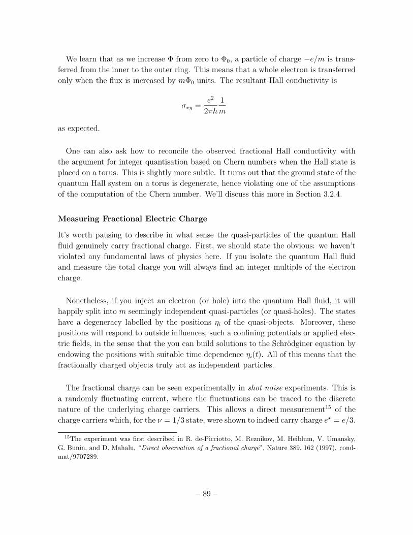
We learn that as we increase Φ from zero to Φ0, a particle of charge −e/m is trans-
ferred from the inner to the outer ring. This means that a whole electron is transferred
only when the flux is increased by mΦ0 units. The resultant Hall conductivity is
σxy =e2
2π~
1
m
as expected.
One can also ask how to reconcile the observed fractional Hall conductivity with
the argument for integer quantisation based on Chern numbers when the Hall state is
placed on a torus. This is slightly more subtle. It turns out that the ground state of the
quantum Hall system on a torus is degenerate, hence violating one of the assumptions
of the computation of the Chern number. We’ll discuss this more in Section 3.2.4.
Measuring Fractional Electric Charge
It’s worth pausing to describe in what sense the quasi-particles of the quantum Hall
fluid genuinely carry fractional charge. First, we should state the obvious: we haven’t
violated any fundamental laws of physics here. If you isolate the quantum Hall fluid
and measure the total charge you will always find an integer multiple of the electron
charge.
Nonetheless, if you inject an electron (or hole) into the quantum Hall fluid, it will
happily split into m seemingly independent quasi-particles (or quasi-holes). The states
have a degeneracy labelled by the positions ηi of the quasi-objects. Moreover, these
positions will respond to outside influences, such a confining potentials or applied elec-
tric fields, in the sense that the you can build solutions to the Schrodginer equation by
endowing the positions with suitable time dependence ηi(t). All of this means that the
fractionally charged objects truly act as independent particles.
The fractional charge can be seen experimentally in shot noise experiments. This is
a randomly fluctuating current, where the fluctuations can be traced to the discrete
nature of the underlying charge carriers. This allows a direct measurement15 of the
charge carriers which, for the ν = 1/3 state, were shown to indeed carry charge e⋆ = e/3.
15The experiment was first described in R. de-Picciotto, M. Reznikov, M. Heiblum, V. Umansky,
G. Bunin, and D. Mahalu, “Direct observation of a fractional charge”, Nature 389, 162 (1997). cond-
mat/9707289.
– 89 –

3.2.2 Introducing Anyons
We’re taught as undergrads that quantum particles fall into two categories: bosons
and fermions. However, if particles are restricted to move in a two-dimensional plane
then there is a loophole to the usual argument and, as we now explain, much more
interesting things can happen16.
Let’s first recall the usual argument that tells us we should restrict to boson and
fermions. We take two identical particles described by the wavefunction ψ(r1, r2).
Since the particles are identical, all probabilities must be the same if the particles are
exchanged. This tells us that |ψ(r1, r2)|2 = |ψ(r2, r1)|2 so that, upon exchange, the
wavefunctions differ by at most a phase
ψ(r1, r2) = eiπαψ(r2, r1) (3.21)
Now suppose that we exchange again. Performing two exchanges is equivalent to a
rotation, so should take us back to where we started. This gives the condition
ψ(r1, r2) = e2iπαψ(r1, r2) ⇒ e2πiα = 1
This gives the two familiar possibilities of bosons (α = 0) or fermions (α = 1).
So what’s the loophole in the above argument? The weak point is the statement that
when we rotate two particles by 360 we should get back to where we came from. Why
should this be true? The answer lies in thinking about the topology of the worldlines
particles make in spacetime.
In d = 3 spatial dimensions (and, if you’re into string theory, higher), the path that
the pair of particles take in spacetime can always be continuously connected to the
situation where the particles don’t move at all. This is the reason the resulting state
should be the same as the one before the exchange. But in d = 2 spatial dimensions,
this is not the case: the worldlines of particles now wind around each other. When
particles are exchanged in an anti-clockwise direction, like this
16This possibility was first pointed out by Jon Magne Leinaas and Jan Myrheim, “On the Theory
of Identical Particles”, Il Nuovo Cimento B37, 1-23 (1977). This was subsequently rediscovered by
Frank Wilczek in “Quantum Mechanics of Fractional-Spin Particles”, Phys. Rev. Lett. 49 (14) 957
(1982).
– 90 –

the worldlines get tangled. They can’t be smoothly continued into the worldlines of
particles which are exchanged clockwise, like this:
Each winding defines a different topological sector. The essence of the loophole is that,
after a rotation in the two-dimensions, the wavefunction may retain a memory of the
path it took through the phase. This means that may have any phase α in (3.21). In
fact, we need to be more precise: we will say that after an anti-clockwise exchange, the
wavefunction is
ψ(r1, r2) = eiπαψ(r2, r1) (3.22)
After a clockwise exchange, the phase must be e−iπα. Particles with α 6= 0, 1 are referred
to as anyons. This whole subject usually goes by the name of quantum statistics or
fractional statistics. But it has less to do with statistics and more to do with topology.
The Braid Group
Mathematically, what’s going on is that in dimensions d ≥ 3, the exchange of parti-
cles must be described by a representation of the permutation group. But, in d = 2
dimensions, exchanges are described a representation of the braid group.
Suppose that we have n identical particles sitting along a line. We’ll order them
1, 2, 3, . . . , n. The game is that of a street-magician: we shuffle the order of the parti-
cles. The image that their worldlines make in spacetime is called a braid. We’ll only
distinguish braids by their topological class, which means that two braids are consid-
ered the same if we can smoothly change one into the other without the worldlines
crossing. All such braidings form an infinite group which we call Bn
We can generate all elements of the braid group from a simple set of operations,
R1, . . . , Rn−1 where Ri exchanges the ith and (i + 1)th particle in an anti-clockwise
direction. The defining relations obeyed by these generators are
RiRj = RjRi |i− j| > 2
together with the Yang-Baxter relation,
RiRi+1Ri = Ri+1RiRi+1 i = 1, . . . , n− 1
This latter relation is most easily seen by drawing the two associated braids and noting
that one can be smoothly deformed into the other.
– 91 –

R1
R2
R1
R2
R1
R2
Figure 29: The left hand-side of the
Yang-Baxter equation...
Figure 30: ...is topologically equivalent
to the right-hand side.
In quantum mechanics, exchanges of particles act as unitary operators on the Hilbert
space. These will form representations of the braid group. The kind of anyons that
we described above form a one-dimensional representation of the braid group in which
each exchange just gives a phase: Ri = eiπαi . The Yang-Baxter equation then requires
eiπαi = eiπαi+1 which simply tells us that all identical particles must have the same
phase.
One dimensional representation of the braid group are usually referred to as Abelian
anyons. As we’ll show below, these are the kind of anyons relevant for the Laughlin
states. However, there are also more exotic, higher-dimensional representations of the
braid group. These are called non-Abelian anyons. We will discuss some examples in
Section 4.
3.2.3 Fractional Statistics
We will now compute the quantum statistics of quasi-holes in the ν = 1/m Laughlin
state. In passing, we will also provide a more sophisticated argument for the fractional
charge of the quasi-hole. Both computations involve the Berry phase that arises as
quasi-holes move17.
We consider a state of M quasi-holes which we denote as |η1, . . . , ηM〉. The wave-
function is (3.19)
〈z, z|η1, . . . , ηM〉 =M∏
j=1
N∏
i=1
(zi − ηj)∏
k<l
(zk − zl)m e−
∑ni=1 |zi|
2/4l2B
17The structure of this calculation was first described in Daniel Arovas, John Schrieffer and Frank
Wilczek, “Fractional statistics and the quantum Hall effect”, Phys. Rev. Lett. 53, 772 (1984), although
they missed the importance of working with normalised wavefunctions. This was subsequently clarified
by M. Stone. in the collection of reprints he edited called, simply, “The Quantum Hall Effect”.
– 92 –

However, whenever we compute the Berry phase, we should work with the normalised
states. We’ll call this state |ψ〉, defined by
|ψ〉 = 1√Z|η1, . . . , ηM〉
where the normalisation factor is defined as Z = 〈η1, . . . , ηM |η1, . . . , ηM〉, which reads
Z =
∫
∏
d2zi exp
(
∑
i,j
log |zi − ηj |2 +m∑
k,l
log |zk − zl|2 −1
2l2B
∑
i
|zi|2)
(3.23)
This is the object which plays the role of the partition function in the plasma analogy,
now in the presence of impurities localised at ηi.
The holomorphic Berry connection is
Aη(η, η) = −i〈ψ| ∂∂η
|ψ〉 = i
2Z
∂Z
∂η− i
Z〈η| ∂
∂η|η〉
But because |η〉 is holomorphic, and correspondingly 〈η| is anti-holomorphic, we have∂Z∂η
= ∂∂η〈η|η〉 = 〈η| ∂
∂η|η〉. So we can write
Aη(η, η) = − i
2
∂logZ
∂η
Meanwhile, the anti-holomorphic Berry connection is
Aη(η, η) = −i〈ψ| ∂∂η
|ψ〉 = +i
2
∂logZ
∂η
So our task in both cases is to compute the derivative of the partition function (3.23).
This is difficult to do exactly. Instead, we will invoke our intuition for the behaviour
of plasmas.
Here’s the basic idea. In the plasma analogy, the presence of the hole acts like
a charged impurity. In the presence of such an impurity, the key physics is called
screening18. This is the phenomenon in which the mobile charges – with positions zi– rearrange themselves to cluster around the impurity so that its effects cannot be
noticed when you’re suitably far away. More mathematically, the electric potential
due to the impurity is modified by an exponential fall-off e−r/λ where λ is called the
Debye screening length and is proportional to√T . Note that, in order for us to use
this argument, it’s crucial that the artificial temperature (3.8) is high enough that the
plasma lies in the fluid phase and efficient screening can occur.
18You can read about screening in the final section of the lecture notes on Electromagnetism.
– 93 –

Whenever such screening occurs, the impurities are effectively hidden at distances
much greater than λ. This means that the free energy of the plasma is independent of
the positions of the impurities, at least up to exponentially small corrections. This free
energy is, of course, proportional to logZ which is the thing we want to differentiate.
However, there are two ingredients missing: the first is the energy cost between the
impurities and the constant background charge; the second is the Coulomb energy
between the different impurities. The correct potential energy for the plasma with M
impurities should therefore be
U(zk; ηi) = −m2∑
k<l
log
( |zk − zl|lB
)
−m∑
k,i
log
( |zi − ηi|lB
)
−∑
i<j
log
( |ηi − ηj |lB
)
+m
4l2B
N∑
k=1
|zk|2 +1
4l2B
M∑
i=1
|ηi|2 (3.24)
The corrected plasma partition function is then
∫
∏
d2zi e−βU(zi;η) = exp
(
− 1
m
∑
i<j
log |ηi − ηj |2 +1
2ml2B
∑
i
|ηi|2)
Z
As long as the distances between impurities |ηi− ηj | are greater than the Debye length
λ, the screening argument tells us that this expression should be independent of the
positions ηi for high enough temperature. In particular, as we described previously, the
temperature β = 2/m relevant for the plasma analogy is high enough for screening as
long as m . 70 . This means that we must have
Z = C exp
(
1
m
∑
i<j
log |ηi − ηj|2 −1
2ml2B
∑
i
|ηi|2)
for some constant C which does not depend on ηi. This gives some idea of the power
of the plasma analogy. It looks nigh on impossible to perform the integrals in (3.23)
directly; yet by invoking some intuition about screening, we are able to write down the
answer, at least in some region of parameters.
The Berry connections over the configuration space ofM quasi-holes are then simple
to calculate: they are
Aηi = − i
2m
∑
j 6=i
1
ηi − ηj+
iηi4ml2B
(3.25)
– 94 –

η3
η2
η1 η3η1
η2
Figure 31: The path taken to compute
the fractional charge of the quasi-hole...
Figure 32: ...and the path to compute
the fractional statistics.
and
Aηi = +i
2m
∑
j 6=i
1
ηi − ηj− iηi
4ml2B(3.26)
where we stress that these expressions only hold as long as the quasi-holes do not get
too close to each other where the approximation of complete screening breaks down.
We can now use these Berry connections to compute both the charge and statistics of
the quasi-hole.
Fractional Charge
Let’s start by computing the charge of the anyon. The basic idea is simple. We pick
one of the quasi-holes — say η1 ≡ η — and move it on a closed path C. For now we
choose a path which does not enclose any of the other anyons. This ensures that only
the second term in the Berry phase contributes,
Aη =iη
4ml2Band Aη = − iη
4ml2B
After traversing the path C, the quasi-hole will return with a phase shift of eiγ, given
by the Berry phase
eiγ = exp
(
−i∮
C
Aηdη +Aηdη
)
(3.27)
This gives the Berry phase
γ =eΦ
m~(3.28)
where Φ is the total magnetic flux enclosed by the path C. But there’s a nice interpre-
tation of this result: it’s simply the Aharonov-Bohm phase picked up by the particle.
As described in Section 1.5.3, a particle of charge e⋆ will pick up phase γ = e⋆Φ/~.
Comparing to (3.28), we learn that the charge of the particle is indeed
e⋆ =e
m
as promised.
– 95 –

Fractional Statistics
To compute the statistics, we again take a particular quasi-hole — say η1 — on a
journey, this time on a path C which encloses one other quasi-hole, which we’ll take
to be η2. The phase is once again given by (3.27) where, this time, both terms in the
expressions (3.25) and (3.26) for Aη and Aη contribute. The second term once again
gives the Aharonov-Bohm phase; the first term tells us about the statistics. It is
eiγ = exp
(
− 1
2m
∮
C
dη1η1 − η2
+ h.c.
)
= e2πi/m
This is the phase that arises from one quasi-hole encircling the other. But the quantum
statistics comes from exchanging two objects, which can be thought of as a rotating by
180 rather than 360. This means that, in the notation of (3.22), the phase above is
e2πiα = e2πi/m ⇒ α =1
m(3.29)
Note that for a fully filled Landau level, with m = 1, the quasi-holes are fermions.
(They are, of course, actual holes). But for a fractional quantum Hall state, the quasi-
holes are anyons.
Suppose now that we put n quasi-holes together and consider this as a single object.
What are its statistics? If we exchange two such objects, then each quasi-hole in the
first bunch gets exchanged with each quasi-hole in the second bunch. The net result is
that the statistical parameter for n quasi-holes is α = n2/m (recall that the parameter
α is defined mod 2). Note that α does not grow linearly with n. As a check, suppose
that we put m quasi-holes together to reform the original particle that underlies the
Hall fluid. We get α = m2/m = m which is a boson for m even and a fermion for m
odd.
There’s a particular case of this which is worth highlighting. The quasi-particles in
the m = 2 bosonic Hall state have statistical parameter α = 1/2. They are half-way
between bosons and fermions and sometimes referred to as semions. Yet two semions
do not make a fermion; they make a boson.
More generally, it’s tempting to use this observation to argue that an electron can
only ever split into an odd number of anyons. This argument runs as follow: if an
electron were to split into an even number of constituents n, each with statistical
parameter α, then putting these back together again would result in a particle with
statistical parameter n2α. The argument sounds compelling. However, as we will see
in Section 4, there is a loop hole!
– 96 –

While the fractional charge of quasi-holes has been measured experimentally, a direct
detection of their fractional statistics is more challenging. There have been a number of
proposed (and performed) experiments using interferometry to demonstrate but their
conclusions remain open to interpretation.
A Slightly Different Viewpoint
There is a slightly different way of presenting the calculation. It will offer nothing
new here, but often appears in the literature as it proves useful when discussing more
complicated examples. The idea is that we consider a wavefunction that already has
the interesting η dependence built in. So, instead of (3.19), we work with
ψ =∏
a<b
(ηa − ηb)1/m
N∏
a,i
(zi − ηa)∏
k<l
(zk − zl)m e−
∑i |zi|
2/4l2B−∑
a |ηa|2/4ml2B (3.30)
This wavefunction is cooked up so that the associated probability distribution is given
precisely by the partition function with energy (3.24) and hence has no dependence
on η and η. This means that the Berry connection for this wavefunction has only the
second terms in (3.25) and (3.26), corresponding to the Aharonov-Bohm effect due to
the background magnetic field. The term in the Berry connection that was responsible
for fractional statistics is absent. But this doesn’t mean that the physics has changed.
Instead, this phase is manifest in the form of the wavefunction itself, which is no longer
single-valued in ηa. Indeed, if η1 encircles a neighbouring point η2, the wavefunction
pick up a phase e2πi/m, so exchanging two quasi-holes gives the phase eiπ/m.
Of course, this approach doesn’t alleviate the need to determine the Berry phase
arising from the exchange. You still need to compute it to check that it is indeed zero.
3.2.4 Ground State Degeneracy and Topological Order
In this section we describe a remarkable property of the fractional quantum Hall states
which only becomes apparent when you place them on a compact manifold: the number
of ground states depends on the topology of the manifold. As we now explain, this is
intimately related to the existence of anyonic particles.
Consider the following process on a torus. We create from the vacuum a quasi-
particle – quasi-hole pair. We then separate this pair, taking them around one of the
two different cycles of the torus as shown in the figure, before letting them annihilate
again. We’ll call the operator that implements this process T1 for the first cycle and T2for the second.
– 97 –

T1T2
Figure 33: Taking a quasi-hole (red) and
quasi-particle (blue) around one cycle of
the torus
Figure 34: ...or around the other.
Now suppose we take the particles around one cycle and then around the other.
Because the particles are anyons, the order in which we do this matters: there is a
topological difference between the paths taken. Indeed, you can convince yourself that
T1T2T−11 T−1
2 is equivalent to taking one anyon around another: the worldlines have
linking number one. This means that the Ti must obey the algebra
T1T2 = e2πi/m T2T1 (3.31)
But such an algebra of operators can’t be realised on a single vacuum state. This imme-
diately tells us that the ground state must be degenerate. The smallest representation
of (3.31) has dimension m, with the action
T1|n〉 = e2πni/m|n〉T2|n〉 = |n+ 1〉
The generalisation of this argument to a genus-g Riemann surface tells us that the
ground state must have degeneracy mg. Notice that we don’t have to say anything
about the shape or sizes of these manifolds. The number of ground states depends only
on the topology!
It is also possible to explicitly construct the analog of the Laughlin states on a torus
in terms of Jacobi theta functions and see that there are indeed m such states.
Before we proceed, we note that this resolves a puzzle. In Section 2.2.4, we described
a topological approach to the integer quantum Hall effect which is valid when space
is a torus. With a few, very mild, assumptions, we showed that the Hall conductivity
is equal to a Chern number and must, therefore, be quantised. In particular, this cal-
culation made no assumption that the electrons were non-interacting: it holds equally
well for strongly interacting many-body systems. However, one of the seemingly mild
assumptions was that the ground state was non-degenerate. As we’ve seen, this is not
true for fractional quantum Hall states, a fact which explains how these states avoid
having integer Hall conductivity.
– 98 –

Topological Order
We’ve seen in this section that the Laughlin states have a number of very special
properties. One could ask: how can we characterise these states? This is an old
and venerable question in condensed matter physics and, for most systems, has an
answer provided by Landau. In Landau’s framework, different states of matter are
characterised by their symmetries, both those that are preserved by the ground state
and those that are broken. This is described using order parameters of the kind that
we met in the lectures on Statistical Physics when discussing phase transitions.
However, the quantum Hall fluids fall outside of this paradigm. There is no symmetry
or local order parameter that distinguishes quantum Hall states. It turns out that there
is a non-local order parameter, usually called “off-diagonal long-range order” and this
can be used to motivate a Ginzburg-Landau-like description. We will describe this in
Section 5.3.2 but, as we will see, it is not without its pitfalls.
Instead, Wen19 suggested that we should view quantum Hall fluids as a new type of
matter, characterised by topological order. The essence of the proposal is that quantum
states can be characterised their ground state degeneracy and the way in which these
states transform among themselves under operations like (3.31).
3.3 Other Filling Fractions
So far, we have only described the quantum Hall states at filling fraction ν = 1/m.
Clearly there are many more states that are not governed by the Laughlin wavefunction.
As we now show, we can understand many of these by variants of the ideas above.
A Notational Convention
Before we proceed, let’s quickly introduce some new notation. All wavefunctions in the
lowest Landau level come with a common exponential factor. It gets tiresome writing
it all the time, so define
ψ(z, z) ∼ ψ(z)e−∑n
i=1 |zi|2/4l2B
where ψ(z) is a holomorphic function. In what follows we will often just write ψ(z).
Be warned that many texts drop the exponential factor in the wavefunctions but don’t
give the resulting object a different name.
19The original paper is Xiao-Gang Wen, “Topological Orders in Rigid States”, Int. J. Mod. Phys.
B4, 239 (1990), available at Xiao-Gang’s website.
– 99 –

3.3.1 The Hierarchy
We saw in Section 3.2.1 how one can induce quasi-hole (or quasi-particle) states by
introducing a local excess (or deficit) of magnetic field through a solenoid. We could
also ask what happens if we change the magnetic field in a uniform manner so that the
system as a whole moves away from ν = 1/m filling. For definiteness, suppose that we
increase B so that the filling fraction decreases. It seems plausible that for B close to
the initial Laughlin state, the new ground state of the system will contain some density
of quasi-holes, arranged in some, perhaps complicated, configuration. The key idea of
this section is that these quasi-holes might themselves form a quantum Hall state. Let’s
see how this would work.
We know that Laughlin states take the form
ψ ∼∏
i<j
(zi − zj)m
where m is odd for fermions and even for bosons. What would a Laughlin state look like
for anyons with positions ηi and statistical parameter α? To have the right statistics,
the wavefunctions must take the form
ψ ∼N∏
i<j
(ηi − ηj)2p+α
with p a positive integer. As we’ve seen, above the ν = 1/m state, quasi-holes have
statistics α = 1/m while quasi-particles have statistics α = −1/m. It’s simple to
repeat our previous counting of the filling fraction, although now we need to be more
careful about what we’re counting. The maximum angular momentum of a given quasi-
excitation is N(2p ± 1m) so the area of the droplet is A ≈ 2π(2p ± 1
m)N(ml2B) where
the usual magnetic length l2B = ~/eB is now replaced by ml2B because the charge of the
quasi-excitations is q = ±e/m. The number of electron states in a full Landau level is
AB/Φ0 and each can be thought of as made of m quasi-things. So the total number of
quasi-thing states in a full Landau level is mAB/Φ0 = (2p± 1m)m2N .
The upshot of this is that the quasi-holes or quasi-particles give a contribution to
the filling of electron states
νquasi = ∓ 1
2pm2 ±m
where the overall sign is negative for holes and positive for particles. Adding this to
the filling fraction of the original ν = 1/m state, we have
ν =1
m∓ 1
2pm2 ±m=
1
m± 12p
(3.32)
– 100 –

Note that the filling fraction is decreased by quasi-holes and increased by quasi-particles.
Let’s look at some simple examples. We start with the ν = 1/3 state. The p = 1
state for quasi-particles then gives ν = 2/5 which is one of the more prominent Hall
plateaux. The p = 1 state for quasi-hole gives ν = 2/7 which has also been observed;
while not particularly prominent, it’s harder to see Hall states at these lower filling
fractions.
Now we can go further. The quasi-objects in this new state can also form quantum
Hall states. And so on. The resulting fillings are given by the continuous fractions
ν =1
m±1
2p1 ±1
2p2 ± · · ·
(3.33)
For example, building on the Hall state ν = 1/3, the set of continuous fractions for
quasi-particles with pi = 1 leads to the sequence ν = 2/5 (which is the fraction (3.32)),
followed by ν = 3/7, 4/9, 5/11 and 6/13. This is precisely the sequence of Hall
plateaux shown in the data presented at the beginning of this chapter.
3.3.2 Composite Fermions
We now look at an alternative way to think about the hierarchy known as composite
fermions20. Although the starting point seems to be logically different from the ideas
above, we will see the same filling fractions emerging. Moreover, this approach will
allow us to go further ending, ultimately, in Section 3.3.3 with a striking prediction for
what happens at filling fraction ν = 1/2.
First, some motivation for what follows. It’s often the case that when quantum
systems become strongly coupled, the right degrees of freedom to describe the physics
are not those that we started with. Instead new, weakly coupled degrees of freedom
may emerge. Indeed, we’ve already seen an example of this in the quantum Hall effect,
where we start with electrons but end up with fractionally charged particles.
20This concept was first introduced by Jainendra Jain in the paper“Composite-Fermion Approach
to the Fractional Quantum Hall Effect”, Phys. Rev. Lett. 63 2 (1989). It is reviewed in some detail
in his book called, appropriately, “Composite Fermions”. A clear discussion can also be found in the
review “Theory of the Half Filled Landau Level” by Nick Read, cond-mat/9501090.
– 101 –

The idea of this section is to try to find some new degrees of freedom — these are
the “composite fermions”. However, for the most part these won’t be the degrees of
freedom that are observed in the system. Instead, they play a role in the intermediate
stages of the calculations. (There is an important exception to this statement which is
the case of the half-filled Landau level, described in Section 3.3.3, where the observed
excitations of the system are the composite fermions.) Usually it is difficult to identify
the emergent degrees of freedom, and it’s no different here. We won’t be able to
rigorously derive the composite fermion picture. Instead, we’ll give some intuitive and,
in parts, hand-waving arguments that lead us to a cartoon description of the physics.
But the resulting cartoon is impressively accurate. It gives ansatze for wavefunctions
which are in good agreement with the numerical studies and it provides a useful and
unified way to think about different classes of quantum Hall states.
We start by introducing the idea of a vortex. Usually a vortex is a winding in some
complex order parameter. Here, instead, a vortex will mean a winding in the wavefunc-
tion itself. Ultimately we will be interested in vortices in the Laughlin wavefunction,
but to understand the key physics it’s simplest to revisit the quasi-hole whose wave-
function includes the factor
∏
i
(zi − η)
Clearly the wavefunction now has a zero at the position η. This does two things. First,
it depletes the charge there. This, of course, is what gives the quasi-hole its fractional
charge e/m. But because the lowest Landau level wavefunction is holomorphic, there
is also fixed angular dependence: the phase of the wavefunction winds once as the
position of any particle moves around η. This is the vortex.
The winding of the wavefunction is really responsible for the Berry phase calculations
we did in Section 3.2.3 to determine the fractional charge and statistics of the quasi-
hole. Here’s a quick and dirty explanation. The phase of the wavefunction changes by
2π as a particle moves around the quasi-hole. Which means that it should also change
by 2π when the quasi-hole moves around the particle. So if we drag the quasi-hole
around N = νΦ/Φ0 particles, then the phase changes by γ = 2πN = νeΦ/~. This is
precisely the result (3.28) that we derived earlier. Meanwhile, if we drag one quasi-hole
around a region in which there is another quasi-hole, the charge inside will be depleted
by e/m, so the effective number of particles inside is now N = νΦ/Φ0−1/m. This gives
an extra contribution to the phase γ = −2π/m which we associate the statistics of the
quasi-holes: γ = 2πα = 2π/m so α = 1/m, reproducing our earlier result (3.29). We
stress that all of these results really needed only the vortex nature of the quasi-hole.
– 102 –

Now let’s turn to the Laughlin wavefunction itself
ψm(z) ∼∏
i<j
(zi − zj)m
For now we focus on m odd so that the wavefunction is anti-symmetric and we’re
dealing with a Hall state of fermions. One striking feature is that the wavefunction
has a zero of order m as two electrons approach. This means that each particle can
be thought of as m vortices. Of course, one of these zeros was needed by the Pauli
exclusion principle. Moreover, we needed m zeros per particle to get the filling fraction
right. But nothing forced us to have the other m− 1 zeros sitting at exactly the same
place. This is something special about the Laughlin wavefunction.
Motivated by this observation, we define a composite fermion to be an electron (which
gives rise to one vortex due to anti-symmetry) bound to m − 1 further vortices. The
whole thing is a fermion when m is odd. You’ll sometimes hear composite fermions
described as electrons attached to flux. We’ll describe this picture in the language
of Chern-Simons theory in Section 5 but it’s not overly useful at the moment. In
particular, it’s important to note that the composite fermions don’t carry real magnetic
flux with them. This remains uniform. Instead, as we will see later, they carry a
different, emergent flux.
Let’s try to treat this as an object in its own right and see what behaviour we find.
Consider placing some density n = νB/Φ0 of electrons in a magnetic field and subse-
quently attaching these vortices to make composite fermions. We will first show that
these composite fermions experience both a different magnetic field B⋆ and different
filling fraction ν⋆ than the electrons. To see this, we repeat our Berry phase argument
where we move the composite fermion along a path encircling an area A. The resulting
Berry phase has two contributions,
γ = 2π
(
AB
Φ0
− (m− 1)nA
)
(3.34)
with n the density of electrons. The first term is the usual Aharonov-Bohm phase due
to the total flux inside the electron path. The second term is the contribution from the
electron encircling the vortices: there are m − 1 such vortices attached to each of the
ρA electrons.
When we discussed quasi-holes, we also found a different Aharonov-Bohm phase. In
that context, we interpreted this as a different charge of quasi-particles. In the present
context, one usually interprets the result (3.34) in a different (although ultimately
– 103 –

ν =1∗
ν=1/3
ν =2∗
ν=2/5
Figure 35: The composite fermion picture describes a hierarchy of plateaux around, starting
with ν = 1/3, in terms of the integer quantum Hall effect for electrons bound to two vortices.
equivalent) way: we say that the composite fermions experience a different magnetic
field which we call B⋆. The Aharonov-Bohm phase should then be
γ =2πAB⋆
Φ0⇒ B⋆ = B − (m− 1)nΦ0 (3.35)
Because there is one electron per composite fermion, the density is the same. But
because the magnetic fields experienced by electrons and composite fermions differ, the
filling fractions must also differ: we must have n = ν⋆B⋆/Φ0 = νB/Φ0. This gives
ν =ν⋆
1 + (m− 1)ν⋆(3.36)
This is an interesting equation! Suppose that we take the composite fermions to com-
pletely fill their lowest Landau level, so that ν⋆ = 1. Then we have
ν⋆ = 1 ⇒ ν =1
m
In other words, the fractional quantum Hall effect can be thought of as an integer
quantum Hall effect for composite fermions. That’s very cute! Indeed, we can even see
some hint of this in the Laughlin wavefunction itself which we can trivially rewrite as
ψm(z) ∼∏
i<j
(zi − zj)m−1
∏
k<l
(zk − zl) (3.37)
The second term in this decomposition is simply the wavefunction for the fully-filled
lowest Landau level. We’re going to think of the first term as attaching m− 1 vortices
to each position zi to form the composite fermion.
So far we’ve said a lot of words, but we haven’t actually derived anything new from
this perspective. But we can extract much more from (3.36). Suppose that we fill
– 104 –
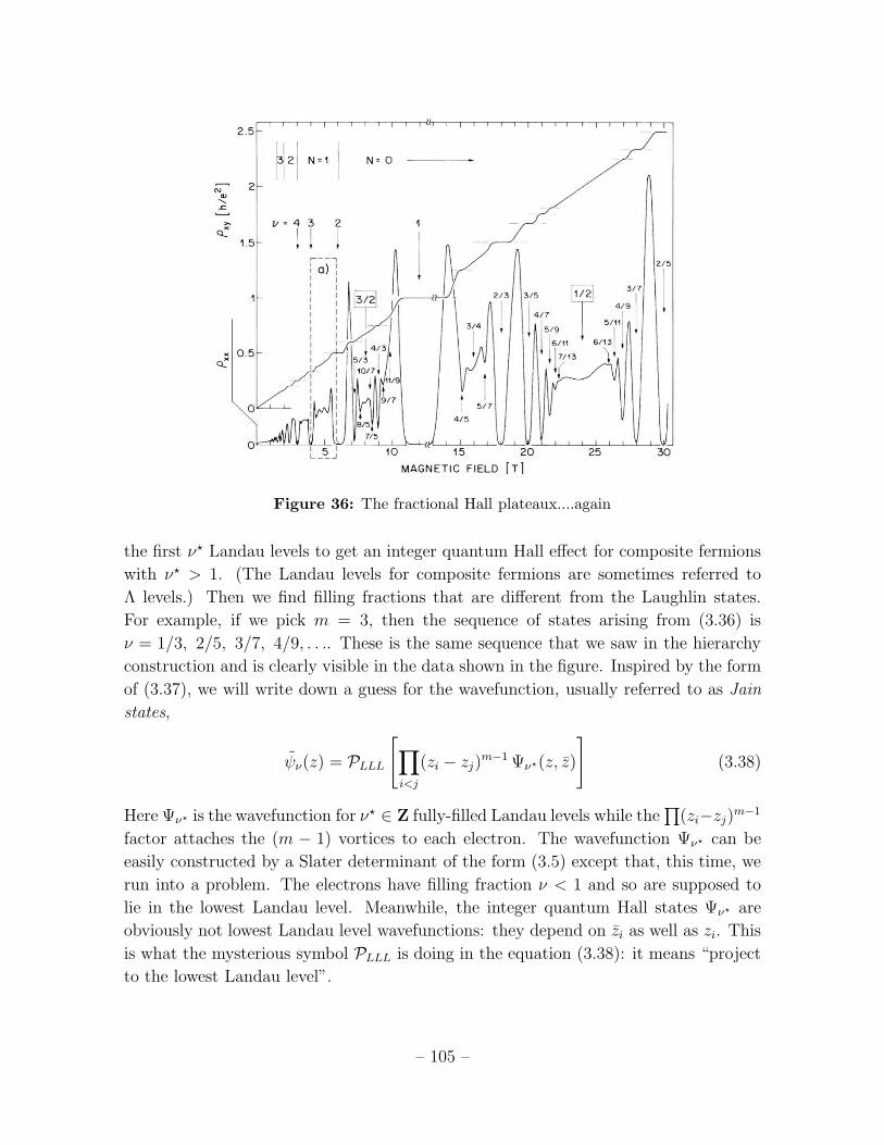
Figure 36: The fractional Hall plateaux....again
the first ν⋆ Landau levels to get an integer quantum Hall effect for composite fermions
with ν⋆ > 1. (The Landau levels for composite fermions are sometimes referred to
Λ levels.) Then we find filling fractions that are different from the Laughlin states.
For example, if we pick m = 3, then the sequence of states arising from (3.36) is
ν = 1/3, 2/5, 3/7, 4/9, . . .. These is the same sequence that we saw in the hierarchy
construction and is clearly visible in the data shown in the figure. Inspired by the form
of (3.37), we will write down a guess for the wavefunction, usually referred to as Jain
states,
ψν(z) = PLLL[
∏
i<j
(zi − zj)m−1Ψν⋆(z, z)
]
(3.38)
Here Ψν⋆ is the wavefunction for ν⋆ ∈ Z fully-filled Landau levels while the∏
(zi−zj)m−1
factor attaches the (m − 1) vortices to each electron. The wavefunction Ψν⋆ can be
easily constructed by a Slater determinant of the form (3.5) except that, this time, we
run into a problem. The electrons have filling fraction ν < 1 and so are supposed to
lie in the lowest Landau level. Meanwhile, the integer quantum Hall states Ψν⋆ are
obviously not lowest Landau level wavefunctions: they depend on zi as well as zi. This
is what the mysterious symbol PLLL is doing in the equation (3.38): it means “project
to the lowest Landau level”.
– 105 –

Operationally, PLLL is defined by moving all factors of zi in [. . .] to the left. We then
make the substitution
zi → 2l2B∂
∂zi(3.39)
Note that this is the same kind of substitution we made in constructing the quasi-
particle wavefunction (3.20). For a small number of particles (N ≈ 20 or so) one
can compute numerically the exact wavefunctions in different filling fractions: the
wavefunctions (3.38) built using the procedure described above have an overlap of
around 99% or so.
Note that it’s also possible to have B⋆ < 0. In this case, we have ρ = −ν⋆B⋆/Φ0 and
the relationship (3.36) becomes
ν =ν⋆
(m− 1)ν⋆ − 1
Then filling successive Landau levels ν⋆ ∈ Z gives the sequence ν = 1, 2/3, 3/5, 4/7, 5/9, . . .
which we again see as the prominent sequence of fractions sitting to the left of ν = 1/2
in the data.
We can also use the projection trick (3.38) to construct excited quasi-hole and quasi-
particle states in these new filling fractions. For each, we can determine the charge and
statistics. We won’t do this here, but we will later revisit this question in Section 5.2.4
from the perspective of Chern-Simons theory.
3.3.3 The Half-Filled Landau Level
The composite fermion construction does a good job of explaining the observed plateaux.
But arguably its greatest success lies in a region where no quantum Hall state is ob-
served: ν = 1/2. (Note that the Laughlin state for m = 2 describes bosons at half
filling; here we are interested in the state of fermions at half filling). Looking at the
data, there’s no sign of a plateaux in the Hall conductivity at ν = 1/2. In fact, there
seems to be a distinct absence of Hall plateaux in this whole region. What’s going on?!
The composite fermion picture gives a wonderful and surprising answer to this. Con-
sider a composite fermion consisting of an electron bound to two vortices. If ν = 1/2, so
that the electrons have density n = B/2Φ0 then the effective magnetic field experienced
by the composite fermions is (3.35)
B⋆ = B − 2nΦ0 = 0 (3.40)
– 106 –

According to this, the composite fermions shouldn’t feel a magnetic field. That seems
kind of miraculous. Looking at the data, we see that the ν = 1/2 quantum Hall state
occurs at a whopping B ≈ 25 T or so. And yet this cartoon picture we’ve built up of
composite fermions suggests that the electrons dress themselves with vortices so that
they don’t see any magnetic field at all.
So what happens to these fermions? Well, if they’re on experiencing a magnetic
field, then they must pile up and form a Fermi sea. The resulting state is simply the
compressible state of a two-dimensional metal. The wavefunction describing a Fermi
sea of non-interacting fermions is well known. If we have N particles, with position
ri, and the N lowest momentum modes are ki, then we place particles in successive
plane-wave states eiki·ri and subsequently anti-symmetrise over particles. The resulting
slater determinant wavefunction is
ψFermi Sea = det(
eiki·rj)
(3.41)
The Fermi momentum is defined to be the highest momentum i.e. kF ≡ |kN |. Once
again, this isn’t a lowest Landau level wavefunction since, in complex coordinates,
k · r = 12(kz + kz). This is cured, as before, by the projection operator giving us the
ground state wavefunction at ν = 1/2,
ψν= 12= PLLL
[
∏
i<j
(zi − zj)2 det
(
eikm·rl)
]
(3.42)
where, as before, the (zi − zj)2 factor captures the fact that each composite fermion
contains two vortices. This state, which describes an interacting Fermi sea, is sometimes
called the Rezayi-Read wavefunction. (Be warned: we will also describe a different
class of wavefunctions in Section 4.2.3 which are called Read-Rezayi states!). There
is a standard theory, due to Landau, about what happens when you add interactions
to a Fermi sea known as Fermi liquid theory. The various properties of the state at
ν = 1/2 and its excitations were studied in this context by Halperin, Lee and Read,
and is usually referred to as the HLR theory21.
There is overwhelming experimental evidence that the ν = 1/2 state is indeed a Fermi
liquid. The simplest way to see this comes when we change the magnetic field slightly
away from ν = 1/2. Then the composite fermions will experience a very small magnetic
field B⋆ as opposed to the original B. We can then see the Fermi surface and measure
kF through standard techniques such as de Haas-van Alphen oscillations. Perhaps the
21The paper is “Theory of the half-filled Landau level”, Phys. Rev. B 47, 7312 (1993).
– 107 –

cleanest demonstration is then to look at excitations above the Fermi surface. Using
simple classical physics, we expect that the particles will move in the usual cyclotron
circles, with x + iy = Reiωt where ω = eB⋆/m⋆. The slight problem here is that we
don’t know m⋆. But if we differentiate, we can relate the radius of the circle to the
momentum of the particle which, in the present case, we can take to be ~kF . We then
get the simple prediction
R =~kFeB⋆
which has been confirmed experimentally.
The Dipole Interpretation
Usually when we build a Fermi sea by filling successive momentum states, it’s obvious
where the momentum comes from. But not so here. The problem is that the electrons
are sitting in the lowest Landau level where all kinetic energy is quenched. The entire
Hamiltonian is governed only by the interactions between electrons,
H = Vint(|ri − rj|)
Typically we take this to be the Coulomb repulsion (3.1) or some toy Hamiltonian of
the kind described in Section 3.1.3. How can we get something resembling momentum
out of such a set-up?
A potential answer comes from looking at the wavefunction (3.41) in more detail.
The plane wave state is ei2(kz+kz). Upon making the substitution (3.39), this includes
the term
exp
(
ikl2B∂
∂z
)
But this is simply a translation operator. It acts by shifting z → z + ikl2B. It means
that in this case we can rewrite the wavefunction (3.42) explicitly in holomorphic form,
ψν= 12= A
[
∏
i
eikizi−|zi|2/4l2B
]
∏
i<j
(
(zi + ikil2B)− (zj + ikjl
2B))2
where A is what’s left of the determinant, and means that we should anti-symmetrise
over all different ways of pairing up ki and zi. Note that, for once, we’ve written the
wavefunction including the exponential factor. The net result is that the zeros of the
wavefunction — which are the vortices — are displaced by a distance |kl2B| from the
electron, in the direction perpendicular to ~k.
– 108 –

d
k
−e +ed
k
+e/2−e/2Figure 37: The composite fermion is a
dipole like this.
Figure 38: Or perhaps like this.
As with much of the discussion on composite fermions, the ideas above are no more
than suggestive. But they have turned out to be useful. Now that we have an extended
object, thinking in terms of a reduced magnetic field is perhaps not so useful since
the two ends can experience different magnetic fields. Instead, we can return to our
original quasi-hole interpretation in which the vortices carry charge. One end then has
two vortices, each with charge +e/2. The other end consists of an electron with charge
−e. The net result is the symmetric, dipole configuration shown in the figure with a
dipole moment ~d, with magnitude proportional to ~k, such that ~d ·~k = 0 and |~d| = ekl2B.
The energy needed to produce such a dipole separation now comes entirely from the
Coulomb interaction V (|d|) which we now interpret as V (|~k|). On rotational grounds,
the expansion of the potential energy should start with a term ∼ |~d|2 for small ~d. This
is the origin of the kinetic energy. The electron will drift along equipotentials of V |~k|),while the vortices experience it as a magnetic field. The net effect is that both ends of
the dipole move in the same direction, ~k with velocity ∂V/∂~k as expected.
We note that, more recently it’s been suggested that it’s better to think of the
displacement as acting on just one of the two vortices bound to the electron22. This
can be justified on the grounds that each electron always accompanies a single zero
because of Pauli exclusion. The end with a single vortex has charge +e/2, while the
end that consists of an electron bound to a single vortex has charge −e+ e/2 = −e/2.We get the same qualitative physics as before, but with |~d| = ekl2B/2 as shown in the
figure. The only difference between these two possibilities lies in the Berry phase that
the dipole acquires as it moves around the Fermi surface. This helps resolve an issue
about particle-hole symmetry at half-filling which we will discuss briefly in Section
5.3.3.
22This was proposed by Chong Wang and Senthil in “Half-filled Landau level, topological insulator
surfaces, and three dimensional quantum spin liquids”, arXiv:1507.08290.
– 109 –

3.3.4 Wavefunctions for Particles with Spin
Until now we’ve neglected the role of spin in the quantum Hall states, arguing that
the Zeeman effect is sufficient to polarise the spin of the electron. Here we describe a
simple generalisation of the Laughlin wavefunction for particles that carry spin23.
We split our particles into two sets. The first set has spin-up, with positions
z1, . . . zN↑ . The second set has spin-down, with positions w1, . . . , wN↓ . Note that each
electron has a fixed spin which is an eigenvalue of Sz: we don’t allow the spin to
fluctuate, nor do we allow the spin to be misaligned from the z-axis. We’ll relax this
condition shortly.
If the two sets of particles didn’t talk to each other, we can trivially take the product
of two Laughlin wavefunctions,
ψ(z, w) =N↑∏
i<j
(zi − zj)m1
N↓∏
k<l
(wk − wl)m2 e−
∑|zi|2/4l2B−
∑|ωi|2/4l2B
Such a state would have filling fraction ν↑ = 1/m1 and ν↓ = 1/m2, giving total filling
fraction ν = ν↑ + ν↓.
Clearly there’s nothing new in these wavefunctions. What’s more, they miss the
interesting physics. As we saw above, the Coulomb interactions are what drives the
state to the Laughlin wavefunction. But these Coulomb interactions are blind to spin.
They must also give correlations between the two sets of electrons. Halperin proposed
to capture this with the simple wavefunction
ψ(z, w) =
N↑∏
i<j
(zi − zj)m1
N↓∏
k<l
(wk − wl)m2
∏
i,k
(zi − wk)n (3.43)
where now ψ means that we’re dropping the exponential factors for both variables.
This set of wavefunctions are characterised by the three integers and usually referred
to as the (m1, m2, n) states, or sometimes as Halperin states.
These wavefunctions have very similar properties to the Laughlin states. In particu-
lar, the relative angular momentum is never less thanm1 between two spin-up particles,
never less than m2 for two down-spin particles and never less than n for particles of
opposite spin. This kind of intuition allows us to build toy Hamiltonians, similar to
those of Section 3.1.3, which have these wavefunctions as ground states.
23These wavefunctions were first introduced by Bert Halperin in “Theory of the quantized Hall
conductance”, Helv. Phys. Acta, 56 (1983).
– 110 –
Let’s now compute the filling fractions of these wavefunctions. Following our calcu-
lation in Section 3.1.1, we’ll look at the highest power of a given spin-up electron, say
z1. We see that this has maximum angular momentum m1N↑ + nN↓ and hence fills
out an area
A↑ = 2π(m1N↑ + nN↓)l2B
Meanwhile, the same computation for the spin-down particles gives us the area
A↓ = 2π(m2N↓ + nN↑)l2B
If we want to focus on the places where both spin-up and spin-down particles intermin-
gle, we should take A↑ = A↓. Clearly for a given state (m1, m2, n) this puts a constraint
on, say, N↓ given N↑. The filling fractions are then
ν↑ =N↑
m1N↑ + nN↓=
m2 − n
m1m2 − n2
ν↓ =N↓
m2N↓ + nN↑=
m1 − n
m1m2 − n2
where, in the second equality, we have used the constraint that follows from choosing
A↑ = A↓. The total filling fraction is then
ν = ν↑ + ν↓ =m1 +m2 − 2n
m1m2 − n2(3.44)
The most prominent states of this kind have the form (m,m, n). These have filling
fractions ν↑ = ν↓ = ν/2 with
ν =2
m+ n(3.45)
Interesting examples include
• (3, 3, 1) with ν = 1/2. Note that this is a genuine quantum Hall state at ν = 1/2,
as opposed to the Fermi liquid state described in Section 3.3.3. It has been seen
in bi-layer samples, in which the z and w coordinate refer to the positions of
particles in the two different layers24.
• (3, 3, 2) with ν = 2/5. This state competes with the spin-polarised Jain state
that occurs at the same filling.
24See Y. Suen et. al, “Observation of a ν = 1/2 Fractional Quantum Hall State in a Double-Layer
Electron System”, Phys. Rev. Lett 68 9 (1992).
– 111 –

Given these states, we could now start to construct quasi-hole and quasi-particle
states for these multi-component wavefunctions. The quasi-holes in the (m,m, n) state
turn out to have charge e/(m+ n). We’ll postpone this discussion to Section 5, where
we’ll see that we can describe both the (m1, m2, n) states and the Jain states of Section
3.3.2 in a unified framework.
Putting Spin Back In
So far, we’ve been calling the different sets of particles “spin-up” and “spin-down”, but
the wavefunctions (3.43) don’t really carry the spin information. For example, there’s
no way to measure the spin of the particle in along the x-axis, as opposed to the z-
axis. However, there’s a simple way to remedy this. We just add the spin information,
σ =↑ or ↓ for each particle and subsequently anti-symmetrise (for fermions) over all
N = N↑ +N↓ particles. For (m,m, n) states, with m > n and N↑ = N↓ = N/2, this is
written as
ψ(z, σ) = A
N∏
i<j
(zi − zj)n∏
1<i<j<N/2
(zi − zj)m−n
∏
N/2+1<k<l<N
(zk − zl)m−n | ↑ . . . ↑ ↓ . . . ↓〉
where A stands for anti-symmetrise over all particles, exchanging both positions and
spins. Since the spin state above is symmetric in the first N/2 spins and the second
N/2 spins, we must have m odd. (For bosons we could symmetrise over all particles
providing m is even).
A particularly interesting class of wavefunction are spin singlets. Given a bunch of
N spins, one simple way to form a spin singlet state is to choose a pairing of particles
— say (12) and (34) and so on — and, for each pair, forming the spin singlet
|12〉 = 1√2
(
| ↑1↓2〉 − | ↓1↑2〉)
Then the spin state |Ψ〉 = |12〉|34〉 . . . |N − 1, N〉 is a spin singlet.
An Aside: Of course, the spin singlet constructed above is not unique. The number
of spin singlet states is given by the Catalan number, N !/(N↑+1)!N↑! where N = 2N↑.
We now want to write a spin singlet quantum Hall wavefunction. (Note that this is
the opposite limit to the Laughlin wavefunctions which were fully spin polarised). Since
the spin singlet state is itself anti-symmetric, we now require, in addition to having m
odd, that n is even. It is then straightforward to construct a spin singlet version of the
– 112 –

(n+ 1, n+ 1, n) Halperin state by writing
ψ(z, w, σ) = A[
N∏
i<j
(zi − zj)n∏
i<j odd
(zi − zj)∏
k<l even
(zk − zl) |12〉|34〉 . . . |N − 1, N〉]
It can be seen to be a spin singlet because the last two factors are just Slater determi-
nants for spin up and spin down respectively, which is guaranteed to form a spin singlet.
Meanwhile, the first factor is a symmetric polynomial and doesn’t change the spin. A
stronger statement, which would require somewhat more group theory to prove, is that
the (n+ 1, n+ 1, n) Halperin states are the only spin singlets.
There is much more interesting physics in these quantum Hall states with spin. In
particular, for the case m = n, the Halperin states become degenerate with others
in which the spins do not lie in along the z-direction and the spin picks up its own
dynamics. The resulting physics is much studied and associated to the phenomenon of
quantum Hall ferromagnetism
– 113 –
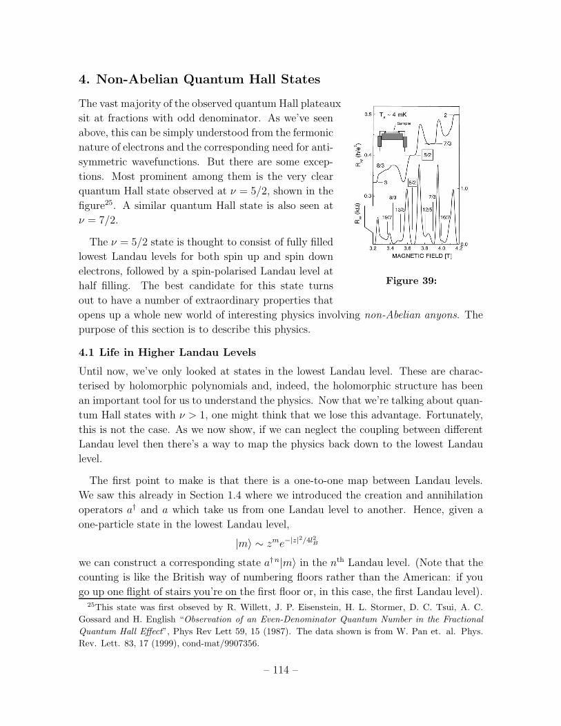
4. Non-Abelian Quantum Hall States
The vast majority of the observed quantum Hall plateaux
Figure 39:
sit at fractions with odd denominator. As we’ve seen
above, this can be simply understood from the fermonic
nature of electrons and the corresponding need for anti-
symmetric wavefunctions. But there are some excep-
tions. Most prominent among them is the very clear
quantum Hall state observed at ν = 5/2, shown in the
figure25. A similar quantum Hall state is also seen at
ν = 7/2.
The ν = 5/2 state is thought to consist of fully filled
lowest Landau levels for both spin up and spin down
electrons, followed by a spin-polarised Landau level at
half filling. The best candidate for this state turns
out to have a number of extraordinary properties that
opens up a whole new world of interesting physics involving non-Abelian anyons. The
purpose of this section is to describe this physics.
4.1 Life in Higher Landau Levels
Until now, we’ve only looked at states in the lowest Landau level. These are charac-
terised by holomorphic polynomials and, indeed, the holomorphic structure has been
an important tool for us to understand the physics. Now that we’re talking about quan-
tum Hall states with ν > 1, one might think that we lose this advantage. Fortunately,
this is not the case. As we now show, if we can neglect the coupling between different
Landau level then there’s a way to map the physics back down to the lowest Landau
level.
The first point to make is that there is a one-to-one map between Landau levels.
We saw this already in Section 1.4 where we introduced the creation and annihilation
operators a† and a which take us from one Landau level to another. Hence, given a
one-particle state in the lowest Landau level,
|m〉 ∼ zme−|z|2/4l2B
we can construct a corresponding state a†n|m〉 in the nth Landau level. (Note that the
counting is like the British way of numbering floors rather than the American: if you
go up one flight of stairs you’re on the first floor or, in this case, the first Landau level).25This state was first obseved by R. Willett, J. P. Eisenstein, H. L. Stormer, D. C. Tsui, A. C.
Gossard and H. English “Observation of an Even-Denominator Quantum Number in the Fractional
Quantum Hall Effect”, Phys Rev Lett 59, 15 (1987). The data shown is from W. Pan et. al. Phys.
Rev. Lett. 83, 17 (1999), cond-mat/9907356.
– 114 –

Similarly, a state of two particles in the lowest Landau level decomposes into a centre
of mass part and a relative part, written as
|M,m〉 ∼ (zi + zj)M(zi − zj)
me−(|zi|2+|zj |2)/4l2B
We can also again construct the corresponding state a†n1 a†n2 |M,m〉 in which each par-
ticle now sits in the nth Landau level.
We’ve already seen in Section 3.1.3 that, if we focus attention to the lowest Landau
level, then the interactions between particles can be characterised by pseudopotentials,
defined by (3.11)
vm =〈M,m|V (|ri − rj|)|M,m〉
〈M,m|M,m〉
For a potential of the form V (|r1 − r2|) which is both translationally and rotationally
invariant, these pseudopotentials depend only on a single integer m.
However, this same argument also holds for higher Landau levels. Once again we
can define pseudopotentials, now given by
v(n)m =〈M,m|ani anj V (|ri − rj|)a†ni a†nj |M,m〉
〈M,m|M,m〉 (4.1)
Of course, these differ from the vn, but otherwise the resulting problem is the same.
The upshot of this is that we can think of particles in the nth Landau level, interacting
through a potential V as equivalent to particles in the lowest Landau level interacting
with a potential given by (4.1). Typically one finds that the values of v(n)m are smaller
than the values of vm for low m. This means that there’s less of a penalty paid for
particles coming close.
Practically speaking, all of this provides us with a handy excuse to continue to work
with holomorphic wavefunctions, even though we’re dealing with higher Landau levels.
Indeed, you may have noticed that we’ve not exactly been careful about what potential
we’re working with! Solving the Schrodinger equation for any realistic potential is way
beyond our ability. Instead, we’re just at the stage of making up reasonable looking
wavefunctions. Given this, the fact that we have to deal with a different potential is
not going to be much of a burden.
Moreover, these ideas also explain how ν = 5/2 can be an incompressible quantum
Hall state while, as we’ve seen, ν = 1/2 is a compressible Fermi liquid state. Both
states must be possible at half filling, but which is chosen depends on the detailed
– 115 –

interactions that the electrons experience. Our first task, then, is to write down the
quantum Hall state for electrons at half filling. In fact, we’ve already seen an example
of this: the (3, 3, 1) state described in Section 3.3.4. But, as we now explain, there is
also another, much more interesting candidate.
4.2 The Moore-Read State
The Moore-Read, or Pfaffian state describes an even number of particles, N , with filling
fraction ν = 1/m. It is given by26
ψMR(z) = Pf
(
1
zi − zj
)
∏
i<j
(zi − zj)m (4.2)
In contrast to the Laughlin state, the wavefunction is anti-symmetric, and hence de-
scribes fermions, for m even. It is symmetric for m odd. To see this, we first need to
answer the question:
What’s a Pfaffian?
Consider a n N × N anti-symmetric matrix, Mij . The determinant of such a matrix
vanishes when N is odd, but when N is even the determinant can be written the square
of an object known as the Pfaffian,
det(M) = Pf(M)2
The Pfaffian is itself a polynomial of degree N/2 in the elements of the matrix, with
integer coefficients.
There are a number of alternative expressions for the Pfaffian. Perhaps the simplest
is to partition N into N/2 pairs of numbers. For, example the simplest such partition
is (12), (34), . . . , (N − 1, N). The Pfaffian then takes the form
Pf(M) = A [M12M34 . . .MN−1,N ] (4.3)
where all the details are hidden in the notation A which means anti-symmetrise on the
indices, i.e. sum over all (N)!
2N/2(N/2)!partitions with ± signs. Equivalently, can be written
as
Pf(M) =1
2N/2(N/2)!
∑
σ
sign(σ)
N/2∏
k=1
Mσ(2k−1),σ(2k)
26This state was proposed by Greg Moore and Nick Read in “NonAbelions in the Fractional Quantum
Hall Effect”, Nucl. Phys B360 362 (1991) which can be found here. This important paper also
introduces the relationship between wavefunctions and conformal field theory described later in these
lectures.
– 116 –

where the sum is over all σ ∈ SN , the symmetric group, and sign(σ) is the signature of
σ.
For example, if we have four particles then
Pf
(
1
zi − zj
)
=1
z1 − z2
1
z3 − z4+
1
z1 − z3
1
z4 − z2+
1
z1 − z4
1
z2 − z3
Of course, the expressions rapidly get longer as N increases. For 6 particles, there are
12 terms; for 8 particles there are 105.
What’s the Physics?
The Pfaffian removes factors of zi − zj compared to the Laughlin wavefunction, but in
a clever way so that ψ is never singular: whenever two particles approach, the Pfaffian
diverges but is compensated by the∏
(zi − zj)m factor.
In particular, for the bosonic m = 1 state, the wavefunction doesn’t vanish when
a pair of particles coincides, but it does vanish when the positions of three particles
become coincident. This means that the m = 1 state is a zero-energy ground state of
the 3-body toy Hamiltonian,
H = A∑
i<j<k
δ2(zi − zj)δ2(zi − zk) (4.4)
Similar toy Hamiltonians can be constructed that have the general-mMoore-Read state
as their ground state.
The presence of the Pfaffian means that the Moore-Read state has fewer zeros than
the Laughlin state, suggesting that the particles are more densely packed. However, the
difference is irrelevant in the thermodynamic N → ∞ limit. To see this, we compute
the filling fraction. There are m(N − 1) powers of z1 in the Laughlin-like factor and
a single 1/z1 factor from the Pfaffian. This tells us that the area of the droplet in the
large N limit is the same as the area of the Laughlin droplet with N particles. We
again have
ν =1
m
as promised.
The case ofm = 1 describes a fully filled Landau level of bosons and may be realisable
using cold atoms in a rotating trap. The case of m = 2 describes a half-filled Landau
level of fermions. This will be our primary focus here.
– 117 –

The View from the Composite Fermion
The Moore-Read wavefunction is crying out to be interpreted in terms of composite
fermions. In this language, the∏
(zi− zj)m factor attaches m vortices to each electron.
If m is even, then the underlying electron was a fermion. Attaching an even number of
vortices leaves it as a fermion. In contrast, if m was odd then the underlying “electron”
was a boson. Attaching an odd number of vortices now turns it into a fermion. Either,
way, the combined object of electron + m vortices is a fermion.
We saw in Section 3.3.3 that for m = 2, attaching the vortices results in a composite
fermion in an effectively vanishing magnetic field. The question is: how should we
interpret the Pfaffian in this language? In fact, there is a very natural interpretation:
the Moore-Read state describes composite fermions which pile up to form a Fermi liquid
and subsequently suffer a BCS pairing instability to superconductivity
More meat can be put on this proposal. Here we skip the meat and offer only some
pertinent facts27. In a conventional superconductor, the spins of the electrons form a
spin singlet. This provides the necessary anti-symmetry of the wavefunction so that
the angular momentum part is symmetric. The simplest choice is that the electron pair
condense in the s-wave. However, our composite fermions all have the same spin so
the anti-symmetry must now come from the angular momentum. The simplest choice
is now that the composite fermion pair condenses in the p-wave. In fact, the relevant
choice of spherical harmonics gives what’s known as a px + ipy superconductor. The
appropriate BCS wavefunction for such a superconductor, in the weak pairing limit,
indeed takes the form of the Pfaffian factor in (4.2).
4.2.1 Quasi-Holes
We can now look at excitations of the Moore-Read state. We will focus on quasi-holes.
One obvious thing to try is to simply repeat what we did for the Laughlin quasi-hole
(3.18) and propose the wavefunction,
ψ(z) =∏
k
(zk − η) Pf
(
1
zi − zj
)
∏
i<j
(zi − zj)m (4.5)
and, indeed, there’s nothing wrong with this. By the same arguments we used before,
the resulting object has charge e/m and can be thought of as the addition of a single
flux quantum or, in the language of (3.3.2), a single vortex.
27This idea was proposed by Martin Greiter, Xiao-Gang Wen and Frank Wilzcek in “On Paired Hall
States”, with all the details provided in the paper by Nick Read and Dmitry Green, “Paired states of
fermions in two dimensions with breaking of parity and time-reversal symmetries, and the fractional
quantum Hall effect”, cond-mat/9906453.
– 118 –

However, in the Moore-Read state (much) more interesting things can happen. The
Laughlin quasi-hole, described by (4.5), can itself split into two! We describe this by
building the positions of the new objects into the Pfaffian part of the wavefunction like
so:
ψ(z) = Pf
(
(zi − η1)(zj − η2) + (zj − η1)(zi − η2)
zi − zj
)
∏
i<j
(zi − zj)m (4.6)
Note that the argument of the Pfaffian remains anti-symmetric, as it must. Multiplying
out the Pfaffian, we see that this state contains the same number of (z − η) factors as
(4.5), but clearly encodes the positions η1 and η2 of two independent objects. We will
refer to these smaller objects as the quasi-holes. When these two quasi-holes coincide,
so η1 = η2, we get back the state (4.5).
This means that the individual quasi-holes in (4.6) can each be thought of as a
half-vortex. They have charge
e⋆ =e
2m
In particular, for the m = 2 state at half-filling, the quasi-holes should have charge
e/4. There are claims that this prediction has been confirmed in the ν = 5/2 state
by shot-noise experiments28, although the results remain somewhat controversial and
are certainly less clean than the analogous experiments in the Abelian quantum Hall
states.
How Many States with 4 Quasi-Holes?
What about multiple quasi-holes? This is where things start to get interesting. Suppose
that we want to write down a wavefunction for 4 quasi-holes. Clearly we need to include
the positions ηα, α = 1, 2, 3, 4 into the elements of the Pfaffian. One simple guess is
the following expression
ψ(12),(34)(z) = Pf(12),(34)(z)∏
i<j
(zi − zj)m (4.7)
where we’ve defined
Pf(12),(34)(z) = Pf
(
(zi − η1)(zi − η2)(zj − η3)(zj − η4) + (i↔ j)
zi − zj
)
28M. Dolev, M. Heiblum, V. Umansky, A. Stern and D. Mahalu, “Observation of a Quarter of an
Electron Charge at the ν = 5/2 Quantum Hall State”, Nature 452, 829-834 (2008).
– 119 –
Indeed, (4.7) is a fine quasi-hole state. But it’s not unique: there was an arbitrariness
in the way split the four quasi-particles into the two groups (12) and (34). This makes
it look as if there are two further states that we can write down,
ψ(13),(24)(z) and ψ(14),(23)(z)
So it looks as if there are three states describing 4 quasi-holes. But this isn’t right. It
turns out that these states are not all linearly independent.
It’s a little fiddly to derive the linear dependence of quasi-hole states, but it’s impor-
tant. Here we’ll derive the result for the simplest case of 4 quasi-holes and then just
state the result for the general case of 2n quasi-holes29. The first step is to note the
relation
(z1 − η1)(z1 − η2)(z2 − η3)(z2 − η4) − (z1 − η1)(z1 − η3)(z2 − η4)(z2 − η2) + (1 ↔ 2)
= (z1 − z2)2(η1 − η4)(η2 − η3) (4.8)
which is simplest to see by noting that the left-hand side indeed vanishes on the roots.
To save space, we introduce some new notation. Define ηαβ = ηα − ηβ and
(12, 34) ≡ (z1 − η1)(z1 − η2)(z2 − η3)(z2 − η4) + (1 ↔ 2)
So that (4.8) reads
(12, 34)− (13, 24) = (z1 − z2)2η14η23
Then, using the definition of the Pfaffian (4.3), we have
Pf(13),(24)(z) = A(
(13, 24)
z1 − z2
(13, 24)
z3 − z4. . .
)
= A(
(12, 34)− (z1 − z2)2η14η23
z1 − z2
(12, 34)− (z3 − z4)2η14η23
z3 − z4. . .
)
= A(
(12, 34)
z1 − z2
(12, 34)
z3 − z4. . .
)
−A(
(z1 − z2)η14η23(12, 34)η14η23
z3 − z4. . .
)
+ A(
(z1 − z2)η14η23(z3 − z4)η14η23(12, 34)η14η23
z5 − z6. . .
)
+ . . .
where the terms that we didn’t write down have factors like (z1−z2)(z3−z4)(z5−z6) andso on. However, in the last term, the anti-symmetrisation acts on the (z1− z2)(z3− z4)
29The proof was first given by Chetan Nayak and Frank Wilczek in “2n Quasihole States Realize
2n−1-Dimensional Spinor Braiding Statistics in Paired Quantum Hall States, cond-mat/9605145. The
derivation above for 4 particles also follows this paper.
– 120 –

factor which vanishes. Indeed, for all the remaining terms we have to anti-symmetrise
a polynomial which is linear in each factor and this too vanishes. We’re left with
Pf(13),(24)(z) = Pf(12),(34)(z)−A(
(z1 − z2)η14η23(12, 34)η14η23
z3 − z4. . .
)
The same kind of calculation also gives
Pf(14),(23)(z) = Pf(12),(34)(z)−A(
(z1 − z2)η13η24(12, 34)η14η23
z3 − z4. . .
)
But this gives the result that we want: it says that there is a linear relation between
the three different Pfaffian wavefunctions.
Pf(12),(34)(z)− Pf(13),(24)(z) =η14η23η13η24
(
Pf(12),(34)(z)− Pf(14),(23)(z))
There are two lessons to take from this. The first is that if we fix the positions ηα of
the four quasi-holes, then there is not a unique state that describes them. Instead, the
state is degenerate. But it’s not as degenerate as we might have thought. There are
only 2 states describing four quasi-holes, rather than the 3 that a naive counting gives.
How Many States with Multiple Quasi-holes?
We can now repeat this for the general situation of 2n quasi-hole. To build a suitable
wavefunction, we first decompose these quasi-particles into two groups of n. For ex-
ample let’s pick (1 . . . n) and (n + 1 . . . 2n) as a particularly obvious choice. Then the
wavefunction takes the form (4.7), but with the Pfaffian component replaced by
Pf
(
(zi − η1)(zi − η2) . . . (zi − ηn)(zj − ηn+1)(zj − ηn+2) . . . (zj − ηn) + (i↔ j)
zi − zj
)
(4.9)
Clearly this again depends on the choice of grouping. The number of ways of placing
2n elements into two groups is
1
2
(2n)!
n!n!
but, as our previous discussion shows, these states are unlikely to be linearly indepen-
dent. The question is: how many linearly independent states are there? It turns out
that the answer is:
dimension of Hilbert space = 2n−1 (4.10)
Obviously this agrees with our answer of 2 when we have four quasi-holes.
– 121 –

A moments thought shows that the counting (4.10) is very peculiar. We’re quite used
to the Hilbert space for a group of particles having a degeneracy when each particle
has an internal degree of freedom. For example, if we have N particles each of spin-1/2
then the total Hilbert space has dimension 2N . But that can’t be what’s going on with
our quasi-holes. We have 2n quasi-holes but an internal Hilbert space of dimension
2n−1. Even ignoring the factor of 2−1 for now, we have many fewer states than could
be accounted for by each particle having it’s own internal degree of freedom.
This simple observation is really the key bit of magic captured by the Moore-Read
excitations. The “internal” degrees of freedom described by the Hilbert space of di-
mension 2n−1 are not associated to any individual quasi-hole and they can’t be seen by
looking at any local part of the wavefunction. Instead they are a property of the entire
collection of particles. It is information stored non-locally in the wavefunction.
Quasi-Holes are Non-Abelian Anyons
Let’s now think about what happens when the quasi-holes are exchanged. As we have
seen, if we have 2n quasi-holes then there are 2n−1 possible ground states. When we
take any closed path in the configuration space of quasi-holes, the state of the system
can come back to itself up to a unitary U(2n−1) rotation. This is an example of the
non-Abelian Berry holonomy discussed in Section 1.5.4. The quasi-holes are referred
to as non-Abelian anyons. (The original suggested name was “non-Abelions”, but it
doesn’t seem to have caught on.)
Our task is to figure out the unitary matrices associated to the exchange of particles.
Conceptually, this task is straightforward. We just need to construct an orthonormal
set of 2n−1 wavefunctions and compute the non-Abelian Berry connection (1.52). In
practice, that’s easier said than done. Recall that in the computation of the Berry
connection for Laughlin quasi-holes we relied heavily on the plasma analogy. This
suggests that to make progress we would need to develop a similar, but more involved,
plasma analogy for the Moore-Read state. The resulting calculations are quite long30.
The good news is that although the calculation is somewhat involved, the end result
is quite simple However, this also suggests that there might be a more physical way to
get to this result. And, indeed there is: it involves returning to the composite fermion
picture.
30The results were conjectured in the ’96 paper by Nayak and Wilczek, but a full proof had to
wait until the work of Parsa Bonderson, Victor Guarie and Chetan Nayak, “Plasma Analogy and
Non-Abelian Statistics for Ising-type Quantum Hall States”, arXiv:1008.5194.
– 122 –

4.2.2 Majorana Zero Modes
Recall that, at ν = 1/2, composite fermions are immune to the background magnetic
field and instead form a Fermi sea. The Moore-Read state arises when these composite
fermions pair up and condense, forming a p-wave superconductor.
This viewpoint provides a very simple way to understand the non-Abelian statistics.
Moreover, the results are general and apply to any other (px + ipy) superconductor.
The unconventional superconductor Sr2RuO4 is thought to fall into this class, and it
may be posisible to construct these states in cold atom systems. (A warning: this last
statement is usually wheeled out for almost anything that people don’t really know
how to build.)
To proceed, we will need a couple of facts about the p-wave superconducting state
that I won’t prove. The first is that, in common with all superconductors, there are
vortices, in which the phase of the condensate winds around the core. Because the
composite electrons condense in pairs, the simplest vortex can carry Φ0/2e flux as
opposed to Φ0/e. For this reason, it’s sometimes called a half-vortex, although we’ll
continue to refer to it simply as the vortex. This will be our quasi-hole.
The second fact that we’ll need is the crucial one, and is special to px + ipy super-
conductors. The vortices have zero modes. These are solutions to the equation for
the fermion field in the background of a vortex. They can be thought of as a fermion
bound to the vortex. Importantly, for these p-wave superconductors, this zero mode is
Majorana31.
A Hilbert Space from Majorana Zero Modes
To explain what a Majorana mode means, we’ll have to work in the language of creation
and annihilation operators for particles which is more familiar in the context of quantum
field theory. We start by reviewing these operators for standard fermions. We define
c†i to be the operator that creates an electron (or, more generally a fermion). Here the
index i labels any other quantum numbers of the electron, such as momentum or spin.
Meanwhile, the conjugate operator ci annihilates an electron or, equivalently, creates a
hole. (In high-energy physics, we’d call this an anti-particle.) These fermionic creation
and annihilation operators obey
ci, c†j = δij and ci, cj = c†i , c†j = 0 (4.11)
which can be thought of as the manifestation of the Pauli exclusion principle.
31A very simple explanation of Majorana fermions in different contexts can be found in Frank
Wilczek’s nice review “Majorana Returns”, Nature Physics 5 614 (2009).
– 123 –

A Majorana particle is a fermion which is its own anti-particle. It can be formally
created by the operator
γi = ci + c†i (4.12)
which clearly satisfies the condition γi = γ†i . From (4.11), we see that these Majorana
operators satisfy
γi, γj = 2δij (4.13)
This is known as the Clifford algebra.
While it’s simple to write down the equation (4.12), it’s much harder to cook up
a physical system in which these excitations exist as eigenstates of the Hamiltonian.
For example, if we’re talking about real electrons then c† creates a particle of charge
−e while c creates a hole of charge +e. This means that γ creates a particle which
is in a superposition of different charges. Usually, this isn’t allowed. However, the
environment in a superconductor makes it possible. Electrons have paired up into
Cooper pairs to form a boson which subsequently condenses. The ground state then
contains a large reservoir of particles which can effectively absorb any ±2e charge. This
means that in a superconductor, charge is conserved only mod 2. The electron and hole
then have effectively the same charge.
Suppose now that we have 2n well-separated vortices, each with their Majorana
zero mode γi. (We’ll see shortly why we restrict to an even number of vortices.) We
fix the positions of the vortices. What is the corresponding Hilbert space? To build
the Hilbert space, we need to take two Majorana modes and, from them, reconstruct
a complex fermion zero mode. To do this, we make an arbitrary choice to pair the
Majorana mode associated to one vortex with the Majorana mode associated to a
different vortex. There’s no canonical way to pair vortices like this but any choice we
make will work fine. For now, let’s pair (γ1, γ2) and (γ3, γ4) and so on. We then define
the complex zero modes
Ψk =1
2(γ2k−1 + iγ2k) k = 1, . . . , n (4.14)
These obey the original fermionic commutation relations
Ψk,Ψ†l = δkl and Ψk,Ψl = Ψ†
k,Ψ†l = 0
The Hilbert space is then constructed in a way which will be very familiar if you’ve
taken a first course on quantum field theory. We first introduce a “vacuum”, or reference
– 124 –

state |0〉 which obeys Ψk|0〉 = 0 for all k. We then construct the full Hilbert space by
acting with successive creation operators, Ψ†k to get
|0〉Ψ†k|0〉
Ψ†kΨ
†l |0〉 (4.15)...
Ψ†1 . . .Ψ
†n|0〉
The sector with p excitations has(
pn
)
possible states. The dimension of the full Hilbert
space is
dimension of Hilbert space = 2n
Note, firstly, that the same comments we made for quasi-hole wavefunctions also apply
here. There’s no way to think of this Hilbert space as arising from local degrees of
freedom carried by each of the 2n vortices. Indeed, one advantage of this approach
is that it demonstrates very clearly the non-local nature of the Hilbert space. Each
individual vortex carries only a Majorana zero mode. But a single Majorana zero mode
doesn’t buy you anything: you need two of them to form a two-dimensional Hilbert
space.
The dimension of the Hilbert space we’ve found here is twice as big as the dimension
(4.10) that comes from counting linearly independent wavefunctions. But it turns out
that there’s a natural way to split this Hilbert space into two. As we’ll see shortly,
the braiding of vortices mixes states with an even number of Ψ† excitations among
themselves. Similarly, states with an odd number of Ψ† excitations also mix among
themselves. Each of these Hilbert spaces has dimension 2n−1. The linearly independent
quasi-hole excitations (4.9) can be thought of as spanning one of these smaller Hilbert
spaces.
Braiding of Majorana Zero Modes
The Majorana zero modes give us a simple way to construct the Hilbert space for our
non-Abelian anyons. They also give us a simple way to see the braiding32.
32This calculation was first done by Dimitry Ivanov in “Non-abelian statistics of half-quantum vor-
tices in p-wave superconductors”, cond-mat/0005069.
– 125 –

Recall from Section 3.2.2 that the braid group is generated by Ri, with i = 1, . . . , 2n−1, which exchanges the ith vortex with the (i+1)th vortex in an anti-clockwise direction.
The action of this braiding on the Majorana zero modes is
Ri :
γi → γi+1
γi+1 → −γiγj → γj j 6= i, i+ 1
where the single minus sign corresponds to the fact that the phase of a Majorana
fermion changes by 2π as it encircles a vortex.
We want to represent this action by a unitary operator — which, with a slight abuse
of notation we will also call Ri — such that the effect of a braid can be written as
RiγjR†i . It’s simple to write down such an operator,
Ri = exp(π
4γi+1γi
)
eiπα =1√2(1 + γi+1γi)e
iπα
To see that these two expressions are equal, you need to use the fact that (γi+1γi)2 = −1,
together with sin(π/4) = cos(π/4) = 1/√2. The phase factor eiπα captures the Abelian
statistics which is not fixed by the Majorana approach. For the Moore-Read states at
filling fraction ν = 1/m, it turns out that this statistical phase is given by
α =1
4m(4.16)
Here, our interest lies more in the non-Abelian part of the statistics. For any state in
the Hilbert space, the action of the braiding is
|Ψ〉 → Ri|Ψ〉Let’s look at how this acts in some simple examples.
Two Quasi-holes
Two quasi-holes give rise to two states, |0〉 and Ψ†|0〉. Written in terms of the complex
fermions, the exchange operator becomes
R =1√2(1 + i− 2iΨ†Ψ)eiπα
from which we can easily compute the action of exchange on the two states
R |0〉 = eiπ/4eiπα|0〉 and RΨ†|0〉 = e−iπ/4eiπαΨ†|0〉 (4.17)
Alternatively, written as a 2×2 matrix, we have R = eiπσ3/4eiπα with σ3 the third Pauli
matrix. We see that each state simply picks up a phase factor as if they were Abelian
anyons.
– 126 –

Four Quasi-holes
For four vortices, we have four states: |0〉, Ψk|0〉 for k = 1, 2, and Ψ†1Ψ
†2|0〉. Meanwhile,
there three generators of the braid group. For the exchanges 1 ↔ 2 and 3 ↔ 4, the
corresponding operators involve only a single complex fermion,
R1 =1√2(1 + γ2γ1)e
iπα =1√2(1 + i− 2iΨ†
1Ψ1)eiπα
and
R3 =1√2(1 + γ4γ3)e
iπα =1√2(1 + i− 2iΨ†
2Ψ2)eiπα
This is because each of these exchanges vortices that were paired in our arbitrary choice
(4.14). This means that, in our chosen basis of states, these operators give rise to only
Abelian phases, acting as
R1 =
eiπ/4
e−iπ/4
eiπ/4
e−iπ/4
eiπα and R3 =
e−iπ/4
e−iπ/4
eiπ/4
eiπ/4
eiπα
Meanwhile, the generator R2 swaps 2 ↔ 3. This is more interesting because these two
vortices sat in different pairs in our construction of the basis states using (4.14). This
means that the operator involves both Ψ1 and Ψ2,
R2 =1√2(1 + γ3γ2) =
1√2
(
1− i(Ψ2 +Ψ†2)(Ψ1 −Ψ†
1))
and, correspondingly, is not diagonal in our chosen basis. Instead, it is written as
R2 =1√2
1 0 0 −i0 1 −i 0
0 −i 1 0
i 0 0 1
(4.18)
Here we see the non-Abelian nature of exchange. Note that, as promised, the states
Ψk|0〉 with an odd number of Ψ excitations transform into each other, while the states
|0〉 and Ψ†1Ψ
†2|0〉 transform into each other. This property persists with an arbitrary
number of anyons because the generators Ri defined in (4.17) always contain one cre-
ation operator Ψ† and one annihilation operator Ψ. It means that we are really de-
scribing two classes of non-Abelian anyons, each with Hilbert space of dimension 2n−1.
– 127 –

The non-Abelian anyons that we have described above are called Ising anyons. The
name is strange as it’s not at all clear at this stage what these anyons have to do with
the Ising model. We will briefly explain the connection in Section 6.3.
Relationship to SO(2n) Spinor Representations
The discussion above has a nice interpretation in terms of the spinor representation
of the rotation group SO(2n). This doesn’t add anything new to the physics, but it’s
simple enough to be worth explaining.
As we already mentioned, the algebra obeyed by the Majorana zero modes (4.13) is
called the Clifford algebra. It is well known to have a unique irreducible representation
of dimension 2n. This can be built from 2× 2 Pauli matrices, σ1, σ2 and σ3 by
γ1 = σ1 ⊗ σ3 ⊗ . . .⊗ σ3
γ2 = σ2 ⊗ σ3 ⊗ . . . σ3
...
γ2k−1 = 1⊗ . . .⊗ 1⊗ σ1 ⊗ σ3 ⊗ . . .⊗ σ3
γ2k = 1⊗ . . .⊗ 1⊗ σ2 ⊗ σ3 ⊗ . . .⊗ σ3
...
γ2n−1 = 1⊗ . . .⊗ 1⊗ σ1
γ2n = 1⊗ . . .⊗ 1⊗ σ2
The Pauli matrices themselves obey σa, σb = 2δab which ensures that the gamma-
matrices defined above obey the Clifford algebra.
From the Clifford algebra, we can build generators of the Lie algebra so(2n). The
rotation in the (xi, xj) plane is generated by the anti-symmetric matrix
Tij =i
4[γi, γj] (4.19)
This is called the (Dirac) spinor representation of SO(2n). The exchange of the ith
and jth particle is represented on the Hilbert space by a π/2 rotation in the (xi, xi+1)
plane,
Rij = exp
(
−iπ2Tij
)
For the generators Ri = Ri,i+1, this coincides with our previous result (4.17).
– 128 –

The spinor representation (4.19) is not irreducible. To see this, note that there is
one extra gamma matrix,
γ2n+1 = σ3 ⊗ σ3 ⊗ . . .⊗ σ3
which anti-commutes with all the others, γ2n+1, γi = 0 and hence commutes with the
Lie algebra elements [γ2n+1, Tij] = 0. Further, we have (γ2n+1)2 = 12n, so γ2n+1 has
eigenvalues ±1. By symmetry, there are n eigenvalues +1 and n eigenvalues −1. We
can then construct two irreducible chiral spinor representations of so(2n) by projecting
onto these eigenvalues. These are the representation of non-Abelian anyons that act
on the Hilbert space of dimension 2n−1.
This, then, is the structure of Ising anyons, which are excitations of the Moore-Read
wavefunction. The Hilbert space of 2n anyons has dimension 2n−1. The act of braiding
two anyons acts on this Hilbert space in the chiral spinor representation of SO(2n),
rotating by an angle π/2 in the appropriate plane.
4.2.3 Read-Rezayi States
In this section, we describe an extension of the Moore-Read states. Let’s first give
the basic idea. We’ve seen that the m = 1 Moore-Read state has the property that it
vanishes only when three or more particles come together. It can be thought of as a
zero-energy ground state of the simple toy Hamiltonian,
H = A∑
i<j<k
δ2(zi − zj)δ2(zj − zk)
This suggests an obvious generalisation to wavefunctions which only vanish when some
group of p particles come together. These would be the ground states of the toy
Hamiltonian
H = A∑
i1<i2<...<ip
δ2(zi1 − zi2)δ2(zi2 − zi3) . . . δ
2(zip−1− zip)
The resulting wavefunctions are called Read-Rezayi states.
To describe these states, let us first re-write the Moore-Read wavefunction in a way
which allows a simple generalisation. We take N particles and arbitrarily divide them
up into two groups. We’ll label the positions of the particles in the first group by
v1, . . . , vN/2 and the position of particles in the second group by w1, . . . , wN/2. Then we
can form the wavefunction
ψCGT (z) = S[
∏
i<j
(vi − vj)2(wi − wj)
2
]
– 129 –

where S means that we symmetrise over all ways of diving the electrons into two groups,
ensuring that we end up with a bosonic wavefunction. The claim is that
ψMR(z) = ψCGT (z)∏
i<j
(zi − zj)m−1
We won’t prove this claim here33. But let’s just do a few sanity checks. At m = 1, the
Moore-Read wavefunction is a polynomial in z of degree N(N/2− 1), while any given
coordinate – say z1 – has at most power N − 2. Both of these properties are easily
seen to hold for ψCGT . Finally, and most importantly, ψCGT (z) vanishes only if three
particles all come together since two of these particles must sit in the same group.
It’s now simple to generalise this construction. Consider N = pd particles. We’ll
separate these into p groups of d particles whose positions we label as w(a)1 , . . . , w
(a)d
where a = 1, . . . , p labels the group. We then form the Read-Rezayi wavefunction34
ψRR(z) = S[
∏
i<j
(w(1)i − w
(1)j )2 . . .
∏
i<j
(w(p)i − w
(p)j )2
]
∏
k<l
(zk − zl)m−1
where, again, we symmetrise over all possible clustering of particles into the p groups.
This now has the property that the m = 1 wavefunction vanishes only if the positions of
p+ 1 particles coincide. For this reason, these are sometimes referred to as p-clustered
states, while the original Moore-Read wavefunction is called a paired state.
Like the Moore-Read state, the Read-Rezayi state describes fermions for m even and
bosons for m odd. The filling fraction can be computed in the usual manner by looking
at the highest power of some given position. We find
ν =p
p(m− 1) + 2
The fermionic p = 3-cluster state at m = 2 has filling fraction ν = 3/5 and is a
promising candidate for the observed Hall plateaux at ν = 13/5. One can also consider
the particle-hole conjugate of this state which would have filling fraction ν = 1−3/5 =
2/5. There is some hope that this describes the observed plateaux at ν = 12/5.
33The proof isn’t hard but it is a little fiddly. You can find it in the paper by Cappelli, Georgiev
and Todorov, “Parafermion Hall states from coset projections of abelian conformal theories”, hep-
th/0009229.34The original paper “Beyond paired quantum Hall states: parafermions and incompressible states
in the first excited Landau level, cond-mat/9809384, presents the wavefunction is a slightly different,
but equivalent form.
– 130 –

Quasi-Holes
One can write down quasi-hole excitations above the Read-Rezayi state. Perhaps un-
surprisingly, such quasi-holes necessarily come in groups of p. The simplest such state
is
ψ(z) = S
p∏
a=1
N/p∏
i=1
(w(a)i − ηa)
p∏
a=1
∏
i<j
(w(a)i − w
(a)j )2
∏
k<l
(zk − zl)m−1
As with the Moore-Read state, when the positions of all p quasi-holes coincide, we get
a Laughlin quasi-hole factor∏
(zi − η). This combined object should have charge νe,
so the individual quasi-holes of the Read-Rezayi state have charge
e⋆ =ν
p=
1
p(m− 1) + 2
What about for more quasi-holes? We can easily write down some candidate wave-
functions simply by including more of the∏
(w − η) type factors in the wavefunction.
But we still have the hard work of figuring out how many of these are linearly inde-
pendent. To my knowledge, this has never been shown from a direct analysis of the
wavefunctions. However, the result is known through more sophisticated techniques
involving conformal field theory that we will briefly describe in Section 6. Perhaps the
most interesting is the case p = 3. Here, the number of linearly independent states of
3n quasi-holes can be shown to be d3n−2, where di are the Fibonacci numbers: d1 = 1,
d2 = 2 and dn+1 = dn + dn−1. For this reason, the anyons in the p = 3 Read-Rezayi
state are referred to as Fibonacci anyons.
Like their Moore-Read counterparts, the Fibonacci anyons are also non-Abelian. In
fact, it turns out that they are the simplest possible non-Abelian anyons. Rather than
describe their properties here, we instead take a small diversion and describe the general
abstract theory behind non-Abelian anyons. We’ll use the Fibonacci and Ising anyons
throughout as examples to illustrate the main points. We will postpone to Section 6
any further explanation of how we know that these are the right anyons to describe the
quasi-holes in quantum Hall states.
4.3 The Theory of Non-Abelian Anyons
This section is somewhat tangential to the main theme of these lectures. Its purpose
is to review a general, somewhat formal, theory that underlies non-Abelian anyons35.
35More details can be found in Chapter 9 of the beautiful set of lectures on Quantum Computation
by John Preskill: http://www.theory.caltech.edu/people/preskill/ph229/
– 131 –

We’ll see that there is an intricate structure imposed on any model arising from the
consistency of exchanging different groups of anyons. As we go along, we’ll try to make
contact with the non-Abelian anyons that we’ve seen arising in quantum Hall systems.
The starting point of this abstract theory is simply a list of the different types of
anyons that we have in our model. We’ll call them a, b, c, etc. We include in this list
a special state which has no particles. This is called the vacuum and is denoted as 1.
4.3.1 Fusion
The first important property we need is the idea of fusion. When we bring two anyons
together, the object that we’re left with must, when viewed from afar, also be one of
the anyons on our list. The subtlety is that we need not be left with a unique type of
anyon when we do this. We denote the possible types of anyon that can arise as a and
b are brought together — of fused — as
a ⋆ b =∑
c
N cab c (4.20)
where N cab is an integer that tells us how many different ways there are to get the anyon
of type c. It doesn’t matter which order we fuse anyons, so a⋆b = b⋆a or, equivalently,
N cab = N c
ba. We can also interpret the equation the other way round: if a specific anyon
c appears on the right of this equation, then there is a way for it to split into anyons
of type a and b.
The vacuum 1 is the trivial state in the sense that
a ⋆ 1 = a
for all a.
The idea that we can get different states when we bring two particles together is a
familiar concept from the theory of angular momentum. For example, when we put two
spin-1/2 particles together we can either get a particle of spin 1 or a particle of spin
0. However, there’s an important difference between this example and the non-Abelian
anyons. Each spin 1/2 particle had a Hilbert space of dimension 2. When we tensor
two of these together, we get a Hilbert space of dimension 4 which we decompose as
2× 2 = 3+ 1
Such a simple interpretation is not available for non-Abelian anyons. Typically, we don’t
think of a single anyon as having any internal degrees of freedom and, correspondingly,
– 132 –
it has no associated Hilbert space beyond its position degree of freedom. Yet a pair of
anyons do carry extra information. Indeed, (4.20) tells us that the Hilbert space Hab
describing the “internal” state of a pair of anyons has dimension
dim(Hab) =∑
c
N cab
The anyons are called non-Abelian whenever N cab ≥ 2 for some a, b and c. The infor-
mation contained in this Hilbert space is not carried by any local degree of freedom.
Indeed, when the two anyons a and b are well separated, the wavefunctions describing
different states in Hab will typically look more or less identical in any local region. The
information is carried by more global properties of the wavefunction. For this reason,
the Hilbert space Hab is sometimes called the topological Hilbert space.
All of this is very reminiscent of the situation that we met when discussing the quasi-
holes for the Moore-Read state, although there we only found an internal Hilbert space
when we introduced 4 or more quasi-holes. We’ll see the relationship shortly.
Suppose now that we bring three or more anyons together. We will insist that the
Hilbert space of final states is independent of the order in which we bring them together.
Mathematically, this means that fusion is associative,
(a ⋆ b) ⋆ c = a ⋆ (b ⋆ c)
With this information, we can extrapolate to bringing any number of n anyons, a1, a2, . . . , antogether. The resulting states can be figured out by iterating the rules above: each c
that can be formed from a1 × a2 can now fuse with a3 and each of their products can
fuse with a4 and so on. The dimension of the resulting Hilbert space Ha1...an is
dim(Ha1...an) =∑
b1,...,bn−2
N b1a1a2
N b2b1a3
. . . Nbn−1
bn−2an(4.21)
In particular, we can bring n anyons of the same type a together. The asymptotic
dimension of the resulting Hilbert space H(n)a is written as
dim(H(n)a ) → (da)
n as n→ ∞
Here da is called the quantum dimension of the anyon. They obey da ≥ 1. The vacuum
anyon 1 always has d1 = 1. Very roughy speaking, the quantum dimension should be
thought of as the number of degrees of freedom carried by in a single anyon. However,
as we’ll see, these numbers are typically non-integer reflecting the fact that, as we’ve
stressed above, you can’t really think of the information as being stored on an individual
anyon.
– 133 –

There’s a nice relationship obeyed by the quantum dimensions. From (4.21), and
using the fact that N cab = N c
ba, we can write the dimension of H(n)a as
dim(H(n)a ) =
∑
b1,...,bn−2
N b1aaN
b2ab1. . . N
bn−1
abn−2=∑
b
[Na]nab
where Na is the matrix with components N cab and in the expression above it is raised
to the nth power. But, in the n → ∞, such a product is dominated by the largest
eigenvalue of the matrix Na. This eigenvalue is the quantum dimension da. There is
therefore an eigenvector e = (e1, . . . , en) satisfying
Nae = dae ⇒ N cabec = daeb
For what it’s worth, the Perron-Frobenius theorem in mathematics deals with eigen-
value equations of this type. Among other things, it states that all the components of
ea are strictly positive. In fact, in the present case the symmetry of N cab = N c
ba tells us
what they must be. For the right-hand-side to be symmetric we must have ea = da.
This means that the quantum dimensions obey
dadb =∑
c
N cabdc
Before we proceed any further with the formalism, it’s worth looking at two examples
of non-Abelian anyons.
An Example: Fibonacci Anyons
Fibonacci anyons are perhaps the simplest36. They have, in addition to the vacuum
1, just a single type of anyon which we denote as τ . The fusion rules consist of the
obvious τ ⋆ 1 = 1 ⋆ τ = τ together with
τ ⋆ τ = 1⊕ τ (4.22)
So we have dim(H(2)τ ) = 2. Now if we add a third anyon, it can fuse with the single τ
to give
τ ⋆ τ ⋆ τ = 1⊕ τ ⊕ τ
with dim(H(3)τ ) = 3. For four anyons we have dim(H(4)
τ ) = 5. In general, one can show
that dim(H(n+1)τ ) = dim(H(n)
τ ) + dim(H(n−1)τ ). This is the Fibonacci sequence and is
what gives the anyons their name.
36A simple introduction to these anyons can be found in the paper by S. Trebst, M. Troyer, Z. Wang
and A. Ludwig in “A Short Introduction to Fibonacci Anyon Model”, arXiv:0902.3275.
– 134 –

The matrix Nτ , with components N cτb can be read off from the fusion rules
Nτ =
(
0 1
1 1
)
The quantum dimension is the positive eigenvalue of this matrix which turns out to be
the golden ratio.
dτ =1
2(1 +
√5) (4.23)
This, of course, is well known to be the limiting value of dim(H(n+1)τ )/dim(H(n)
τ ).
Another Example: Ising Anyons
Ising anyons contain, in addition to the vacuum, two types which we denote as σ and
ψ. The fusion rules are
σ ⋆ σ = 1⊕ ψ , σ ⋆ ψ = σ , ψ ⋆ ψ = 1 (4.24)
The ψ are somewhat boring; they have dim(H(n)τ ) = 1 for all n. The dimension of the
Hilbert space of multiple σ anyons is more interesting; it depends on whether there are
an even or odd number of them. It’s simple to check that
dim(H(2n)σ ) = dim(H(2n+1)
σ ) = 2n (4.25)
so we have
dψ = 1 and dσ =√2
Of course, we’ve seen this result before. This is the dimension of the Hilbert space
of anyons constructed from Majorana zero modes described in Section 4.2.2. In this
language, we saw that a pair of vortices share a single complex zero mode, leading to
the states |0〉 and Ψ†|0〉. These are identified with the vacuum 1 and the fermion ψ
respectively. The fusion rule ψ ⋆ ψ = 1 then reflects the fact that pairs of composite
fermions have condensed in the ground state.
4.3.2 The Fusion Matrix
Let’s now return to the general theory. The fusion rules (4.20) aren’t all we need to
specify a particular theory of non-Abelian anyons. There are two further ingredients.
The first arises by considering the order in which we fuse particles together.
– 135 –

Suppose that we have three anyons, a, b and c. We first fuse a and b together and,
of all the possibilities allowed by the fusion rules, we get some specific anyon i. We
subsequently fuse i with c and end up with a specific anyon d. All of this is captured
by a fusion tree which looks like this:
a b c
d
i(4.26)
We list the anyons that we start with at the top and then read the tree by working
downwards to see which anyons fuse to which. Alternatively, you could read the tree
by starting at the bottom and thinking of anyons as splittng. Importantly, there can
be several different anyons i that appear in the intermediate channel.
Now suppose that we do the fusing in a different order: we first fuse b with c and
subsequently fuse the product with a. We ask that the end product will again be the
anyon d. But what will the intermediate state be? There could be several different
possibilities j.
a b c
d
j
The question we want to ask is: if we definitely got state i in the first route, which of
the states j appear in the second route. In general, there won’t be a specific state j,
but rather a linear combination of them. This is described graphically by the equation
a b c
d
i=∑
j
(F dabc)ij
a b c
d
j (4.27)
where the coefficients (F dabc)ij are thought of as the coefficients of a unitary matrix,
F dabc, specified by the four anyons a, b, c and d. This is called the fusion matrix.
A comment: in our attempt to keep the notation concise, we’ve actually missed
an important aspect here. If there are more than one ways in which the anyons j can
appear in intermediate states then we should sum over all of them and, correspondingly,
the fusion matrix should have more indices. More crucially, sometimes there will be
– 136 –

multiple ways in which the final state d can appear. This will happen whenever Ndaj ≥
2 for some j. In this case, the the process on the left will typically give a linear
combination of the different d states on the right. The fusion matrix should also
include indices which sum over these possibilities.
The fusion matrices are extra data needed to specify the structure of non-Abelian
anyons. However, they can’t be chosen arbitrarily: there are consistency relations
which they must satisfy. For some simple theories, this is sufficient to determine the
fusion matrix completely given the fusion rules.
The consistency condition comes from considering four anyons fusing to an end prod-
uct. To avoid burgeoning alphabetical notation, we’ll call the initial anyons 1, 2, 3 and
4 and the final anyon 5. (The notation is not ideal because the anyon 1 does not mean
the vacuum here!) We start with some fusion process in which the anyons are fused in
order, with fixed intermediate states i and j, like this
i
j
1 2 3
5
4
Now we consider reversing the order of fusion. We can do this in two different paths
which is simplest to depict in a graphical notation, known as the pentagon diagram,
j
1 3
5
4
m
2 1 3
5
42
m
lFim4
5
1 2
5
4
i k
3Fi345
F12k5
i
j
1 2 3
5
4
F123j
1
5
42 3
l
k
F234l
The fact that the upper and lower paths in the diagram give the same result means
that the fusion matrix must obey
(F 512k)il(F
5i34)jk =
∑
m
(F l234)mk(F
51m4)jl(F
j123)im (4.28)
– 137 –

These are simply sets of polynomial relations for the coefficients of the fusion matrix.
One might think that fusing more anyons together gives further consistency rules. It
turns out that these all reduce to the pentagon condition above. Let’s look at what
this means for our two favourite examples.
The Fusion Matrix for Fibonacci Anyons
For Fibonacci anyons, the interesting constraint comes from when all external particles
are τ . The pentagon equation (4.28) then reads
(F τττk)il(F
τiττ )jk =
∑
m
(F lτττ )mk(F
ττmτ )jl(F
jτττ )im
Things simplify further by noting that all fusion matrices F dabc are simply given by the
identity whenever a, b, c or d are equal to the vacuum state. (This is always true when
a, b or c is equal to the vacuum state and, for Fibonacci anyons, holds also when d is
the vacuum state). The only non-trivial matrix is F ττττ . If we set j, k = τ and i, l = 1
in the above equation, we get
(F ττττ )11 = (F τ
τττ )τ1(Fττττ )1τ
Combined with the fact that F ττττ is unitary, this constraint is sufficient to determine
the fusion matrix completely. It is
F ττττ =
(
d−1τ d
−1/2τ
d−1/2τ −d−1
τ
)
(4.29)
where we previously calculated (4.23) that the quantum dimension dτ = (1 +√5)/2,
the golden ratio.
The Fusion Matrix for Ising Anyons
The pentagon constraint can also be studied for Ising anyons. It’s a little more com-
plicated37. You can check that a solution to the pentagon equation (4.28) is given by
fusion matrices F σσψσ = F σ
ψσψ = −1 and
(F σσσσ)ij =
1√2
(
1 1
1 −1
)
(4.30)
where the i, j indices run over the vacuum state 1 and the fermion ψ.
37Details can be found in Alexei Kitaev’s “Anyons in an exactly solved model and beyond”, cond-
mat/0506438.
– 138 –

We’d now like to make contact with what we learned in Section 4.2. How do we
think about this fusing matrix in the context of, say, Majorana zero modes? In fact,
there seems to be mismatch from the off, because the fusion matrix starts with three
anyons fusing to one, while the Majorana zero modes naturally came in pairs, meaning
that we should start with an even number of vortices.
We can, however, interpret the original fusion diagram (4.26) in a slightly different
way. We fuse a and b to get anyon i, but (tilting out heads), the diagram also says that
fusing c and d should give the same type of anyon i. What does this mean in terms of
our basis of states (4.15)? The obvious interpretation is that state |0〉 is where both
have fused to 1; the state Ψ†1|0〉 is where the first and second anyon have fused to give
ψ while the third and fourth have fused to give 1; the state Ψ†1|0〉 is the opposite; and
the state Ψ†1Ψ
†2|0〉 is where both have fused to give ψ anyons. All of this means that the
diagram (4.26) with i = 1 is capturing the state |0〉 of four anyons, while the diagram
with i = ψ is capturing the state Ψ†1Ψ
†2|0〉.
Now let’s think about the right-hand side of equation (4.27). This time anyons a and
d fuse together to give a specific anyon j, while b and c fuse together to give the same
anyon j. In terms of Majorana zero modes, we should now rebuild our Hilbert space,
not using the original pairing (4.14), but instead using
Ψ1 =1
2(γ1 + iγ4) and Ψ2 =
1
2(γ3 − iγ2)
and we now construct a Hilbert space built starting from |0〉 satisfying Ψk|0〉 = 0. The
diagram with j = 1 corresponds to |0〉 while the diagram with j = ψ corresponds to
Ψ†1Ψ
†2|0〉. We want to find the relationship between these basis. It’s simple to check
that the unitary map is indeed given by the fusion matrix (4.30).
4.3.3 Braiding
The second important process is a braiding of two anyons. We can do this in two
different ways:
clockwise or anti-clockwise
Suppose that we fuse two anyons a and b together to get c. We then do this again,
but this time braiding the two anyons in an anti-clockwise direction before fusing. The
– 139 –

resulting states are related by the R-matrix, defined by
b a
c
= Rcab
c
ab
If N cab = 1, so that there only a single option for the final anyon, then Rc
ab is simply
a complex phase. However, if N cab ≥ 2, so that there are several different ways of
getting the final anyon c, then there’s no reason we should get the same state after
the exchange. In this case, the R-matrix is a genuine matrix of size N cab × N c
ab and we
should be summing over all possible final states on the right-hand side.
There are further consistency relations that come from reversing the operations of
fusion and braiding. Again, these are best described graphically although the resulting
pictures tend to have lots of swirling lines unless we first introduce some new notation.
We’ll write the left-hand side of the R-matrix equation above as
b a
c
≡
c
a b= Rc
ab
c
ab
Now the consistency relation between fusion matrices and R-matrices arise from the
following hexagon diagram
k
1 32
i
4
R
1 2 3
4
j
3 12
j
4
R
k
2 1 3
4F
F F
R
i
1 2 3
4
2 3 1
4
In equations, this reads
– 140 –

Rk13(F
4213)kiR
i12 =
∑
j
(F 4231)kjR
4j1(F
4123)ji (4.31)
It turns out that the pentagon (4.28) and hexagon (4.31) equations are the only con-
straints that we need to impose on the system. If, for a given set of fusion rules (4.20),
we can find solutions to these sets of polynomial equations then we have a consistent
theory of non-Abelian anyons.
The R-Matrix for Fibonacci Anyons
Let’s see how this works for Fibonacci anyons. We want to compute two phases: R1ττ
and Rτττ . (When either of the lower indices on R is the vacuum state, it is equal to 1.)
We computed the fusion matrix F = F ττττ in (4.29). The left-hand side of the equation
is then
RkττFkiR
iττ = Fk1F1i + FkτFτiR
τττ
Note also our choice of notation has become annoying: in the equation above 1 means
the vacuum, while in (4.31) it refers to whatever external state we chose to put there.
(Sorry!) The equation above must hold for each k and i; we don’t sum over these indices.
This means that it is three equations for two unknowns and there’s no guarantee that
there’s a solution. This is the non-trivial part of the consistency relations. For Fibonacci
anyons, it is simple to check that there is a solution. The phases arising from braiding
are:
R1ττ = e4πi/5 and Rτ
ττ = −e2πi/5
The R-Matrix for Ising Anyons
For Ising anyons, the consistency relations give
R1σσ = e−iπ/8 and Rσ
σσ = e−3πi/8
Note firstly that these are just Abelian phases; the non-Abelian part of exchange that
was described by (4.18) for Majorana zero modes is really captured by the fusion matrix
in this more formal notation.
Note also that this doesn’t agree with the result for anyons computed in Section
4.2.2 since these results depended on the additional Abelian statistical parameter α.
(In fact, the results do agree if we take α = ±1/8 or, equivalently filling factor ν = 1/2.)
For general filling factor, the non-Abelian anyons in the Moore-Read state should be
thought of as attached to further Abelian anyons which shifts this phase.
– 141 –
4.3.4 There is a Subject Called Topological Quantum Computing
There has been a huge surge of interest in non-Abelian anyons over the past 15 years,
much of it driven by the possibility of using these objects to build a quantum computer.
The idea is that the Hilbert space of non-Abelian anyons should be thought of as the
collection of qubits, while the braiding and fusion operations that we’ve described above
are the unitary operations that act as quantum gates. The advantage of using non-
Abelian anyons is that, as we’ve seen, the information is not stored locally. This means
that it is immune to decoherence and other errors which mess up calculations since
this noise, like all other physics, arises from local interactions38. This subject goes by
the name of topological quantum computing. I’ll make no attempt to explain this vast
subject here. A wonderfully clear introduction can be found in the lecture notes by
John Preskill.
38This proposal was first made by A. Kitaev in “Fault tolerant quantum computation by anyons ”,
quant-ph/9707021.
– 142 –

5. Chern-Simons Theories
So far we’ve approached the quantum Hall states from a microscopic perspective, look-
ing at the wavefunctions which describe individual electrons. In this section, we take
a step back and describe the quantum Hall effect on a more coarse-grained level. Our
goal is to construct effective field theories which capture the response of the quantum
Hall ground state to low-energy perturbations. These effective theories are known as
Chern-Simons theories39. They have many interesting properties and, in addition to
their role in the quantum Hall effect, play a starring role in several other stories.
Throughout this section, we’ll make very general statements about the kind of low-
energy effective behaviour that is possible, with very little input about the microscopic
properties of the model. As we will see, we will be able to reconstruct many of the
phenomena that we’ve met in the previous chapters.
We will treat the gauge potential Aµ of electromagnetism as a background gauge
field. This means that Aµ is not dynamical; it is only a parameter of the theory which
tells us which electric and magnetic fields we’ve turned on. Further, we will not include
in Aµ the original background magnetic field which gave rise the Hall effect to begin
with. Instead, Aµ will describe only perturbations around a given Hall state, either by
turning on an electric field, or by perturbing the applied magnetic field but keeping the
kind of state (i.e. the filling fraction) fixed.
In the field theory context, Aµ always couples to the dynamical degrees of freedom
through the appropriate current Jµ, so that the action includes the term
SA =
∫
d3x JµAµ (5.1)
This is the field theoretic version of (2.8). Note that the measure∫
d3x means that
we’ve assumed that the current lives in a d = 2 + 1 dimensional slice of spacetime; it
couples to the gauge field Aµ evaluated on that slice. The action SA is invariant under
gauge transformations Aµ → Aµ + ∂µω on account of the conservation of the current
∂µJµ = 0
These two simple equations will be our starting point for writing down effective field
theories that tell us how the system responds when we perturb it by turning on a
background electric or magnetic field.39Two reviews on the Chern-Simons approach to the quantum Hall effect are Tony Zee, “Quantum
Hall Fluids”, cond-mat/9501022, Xiao-Gang Wen “Topological Orders and Edge Excitations in FQH
States”, cond-mat/9506066. The discussion here follows the spirit of the beautiful lectures by Edward
Witten, “Three Lectures on Topological Phases of Matter”, arXiv:1510.07698.
– 143 –

5.1 The Integer Quantum Hall Effect
We start by looking at the integer quantum Hall effect. We will say nothing about
electrons or Landau levels or anything microscopic. Instead, in our attempt to talk
with some generality, we will make just one, seemingly mild, assumption: at low-
energies, there are no degrees of freedom that can affect the physics when the system
is perturbed.
Let’s think about what this assumption means. The first, and most obvious, require-
ment is that there is a gap to the first excited state. In other words, our system is
an insulator rather than a conductor. We’re then interested in the physics at energies
below this gap.
Naively, you might think that this is enough to ensure that there are no relevant
low-energy degrees of freedom. However, there’s also a more subtle requirement hiding
in our assumption. This is related to the existence of so-called “topological degrees of
freedom”. We will ignore this subtlety for now, but return to it in Section 5.2 when we
discuss the fractional quantum Hall effect.
As usual in quantum field theory, we want to compute the partition function. This
is not a function of the dynamical degrees of freedom since these are what we inte-
grate over. Instead, it’s a function of the sources which, for us, is the electromagnetic
potential Aµ. We write the partition function schematically as
Z[Aµ] =
∫
D(fields) eiS[fields;A]/~ (5.2)
where “fields” refer to all dynamical degrees of freedom. The action S could be anything
at all, as long as it satisfies our assumption above and includes the coupling to Aµthrough the current (5.1). We now want to integrate out all these degrees of freedom,
to leave ourselves with a theory of the ground state which we write as
Z[Aµ] = eiSeff [Aµ]/~ (5.3)
Our goal is to compute Seff [Aµ], which is usually referred to as the effective action.
Note, however, that it’s not the kind of action you meet in classical mechanics. It
depends on the parameters of the problem rather than dynamical fields. We don’t use
it to compute Euler-Lagrange equations since there’s no dynamics in Aµ. Nonetheless,
it does contain important information since, from the coupling (5.1), we have
δSeff [A]
δAµ(x)= 〈Jµ(x)〉 (5.4)
This is telling us that the effective action encodes the response of the current to electric
and magnetic fields.
– 144 –

Since we don’t know what the microscopic Lagrangian is, we can’t explicitly do the
path integral in (5.2). Instead, our strategy is just to write down all possible terms
that can arise and then focus on the most important ones. Thankfully, there are many
restrictions on what the answer can be which means that there are just a handful of
terms we need to consider. The first restrictions is that the effective action Seff [A] must
be gauge invariant. One simple way to achieve this is to construct it out of electric and
magnetic fields,
E = −1
c∇A0 −
∂A
∂tand B = ∇×A
The kinds of terms that we can write down are then further restricted by other sym-
metries that our system may (or may not) have, such as rotational invariance and
translational invariance.
Finally, if we care only about long distances, the effective action should be a local
functional, meaning that we can write is as Seff [A] =∫
ddx . . . . This property is
extremely restrictive. It holds because we’re working with a theory with a gap ∆E in
the spectrum. The non-locality will only arise at distances comparable to ∼ v~/∆E
with v a characteristic velocity. (This is perhaps most familiar for relativistic theories
where the appropriate scale is the Compton wavelength ~/mc). To ensure that the gap
isn’t breached, we should also restrict to suitably small electric and magnetic fields.
Now we just have to write down all terms in the effective action that satisfy the above
requirements. There’s still an infinite number of them but there’s a simple organising
principle. Because we’re interested in small electric and magnetic fields, which vary
only over long distances, the most important terms will be those with the fewest powers
of A and the fewest derivatives. Our goal is simply to write them down.
Let’s first see what all of this means in the context of d = 3 + 1 dimensions. If we
have rotational invariance then we can’t write down any terms linear in E or B. The
first terms that we can write down are instead
Seff [A] =
∫
d4x ǫE · E− 1
µB ·B (5.5)
There is also the possibility of adding a E ·B term although, when written in terms of
Ai this is a total derivative and so doesn’t contribute to the response. (This argument
is a little bit glib; famously the E · B term plays an important role in the subject of
3d topological insulators but this is beyond the scope of these lectures.) The response
(5.4) that follows from this effective action is essentially that of free currents. Indeed,
it only differs from the familiar Lorentz invariant Maxwell action by the susceptibilities
– 145 –

ǫ and µ which are the free parameters characterising the response of the system. (Note
that the response captured by (5.5) isn’t quite the same as Ohm’s law that we met in
Section 1 as there’s no dissipation in our current framework).
The action (5.5) has no Hall conductivity because this is ruled out in d = 3 +
1 dimensions on rotational grounds. But, as we have seen in great detail, a Hall
conductivity is certainly possible in d = 2+ 1 dimensions. This means that there must
be another kind of term that we can write in the effective action. And indeed there
is....
5.1.1 The Chern-Simons Term
The thing that’s special in d = 2+1 dimension is the existence of the epsilon symbol ǫµνρwith µ, ν, ρ = 0, 1, 2. We can then write down a new term, consistent with rotational
invariance. The resulting effective action is Seff [A] = SCS[A] where
SCS[A] =k
4π
∫
d3x ǫµνρAµ∂νAρ (5.6)
This is the famous Chern-Simons term. The coefficient k is sometimes called the level
of the Chern-Simons term.
At first glance, it’s not obvious that the Chern-Simons term is gauge invariant since
it depends explicitly on Aµ. However, under a gauge transformation, Aµ → Aµ + ∂µω,
we have
SCS[A] → SCS[A] +k
4π
∫
d3x ∂µ (ωǫµνρ∂νAρ)
The change is a total derivative. In many situations we can simply throw this total
derivative away and the Chern-Simons term is gauge invariant. However, there are
some situations where the total derivative does not vanish. Here we will have to think
a little harder about what additional restrictions are necessary to ensure that SCS[A]
is gauge invariant. We see that the Chern-Simons term is flirting with danger. It’s
very close to failing the demands of gauge invariance and so being disallowed. The
interesting and subtle ways on which it succeeds in retaining gauge invariance will lead
to much of the interesting physics.
The Chern-Simons term (5.6) respects rotational invariance, but breaks both parity
and time reversal. Here we focus on parity which, in d = 2 + 1 dimensions, is defined
as
x0 → x0 , x1 → −x1 , x2 → x2
– 146 –

and, correspondingly, A0 → A0, A1 → −A1 and A2 → A2. The measure∫
d3x is
invariant under parity (recall that although x1 → −x1, the limits of the integral also
change). However, the integrand is not invariant: ǫµνρAµ∂νAρ → −ǫµνρAµ∂νAρ. This
means that the Chern-Simons effective action with k 6= 0 can only arise in systems that
break parity. Looking back at the kinds of systems we met in Section 2 which exhibit a
Hall conductivity, we see that they all break parity, typically because of a background
magnetic field.
Let’s look at the physics captured by the Chern-Simons term using (5.4). First, we
can compute the current that arises from Chern-Simons term. It is
Ji =δSCS[A]
δAi= − k
2πǫijEi
In other words, the Chern-Simons action describes a Hall conductivity with
σxy =k
2π(5.7)
This coincides with the Hall conductivity of ν filled Landau levels if we identify the
Chern-Simons level with k = e2ν/~.
We can also compute the charge density J0. This is given by
J0 =δSCS[A]
δAi=
k
2πB (5.8)
Recall that we should think of Aµ as the additional gauge field over and above the
original magnetic field. Correspondingly, we should think of J0 here as the change
in the charge density over and above that already present in the ground state. Once
again, if we identify k = e2ν/~ then this is precisely the result we get had we kept ν
Landau levels filled while varying B(x).
We see that the Chern-Simons term captures the basic physics of the integer quantum
Hall effect, but only if we identify the level k = e2ν/~. But this is very restrictive
because ν describes the number of filled Landau levels and so can only take integer
values. Why should k be quantised in this way?
Rather remarkably, we don’t have to assume that k is quantised in this manner;
instead, it is obliged to take values that are integer multiples of e2/~. This follows
from the “almost” part of the almost-gauge invariance of the Chern-Simons term. The
quantisation in the Abelian Chern-Simons term (5.6) turns out to be somewhat sub-
tle. (In contrast, it’s much more direct to see the corresponding quantisation for the
– 147 –

non-Abelian Chern-Simons theories that we introduce in Section 5.4). To see how it
arises, it’s perhaps simplest to place the theory at finite temperature and compute the
corresponding partition function, again with Aµ a source. To explain this, we first need
a small aside about how should think about the equilibrium properties of field theories
at finite temperature.
5.1.2 An Aside: Periodic Time Makes Things Hot
In this small aside we will look at the connection between the thermal partition function
that we work with in statistical mechanics and the quantum partition function that we
work with in quantum field theory. To explain this, we’re going to go right back to
basics. This means the dynamics of a single particle.
Consider a quantum particle of mass m moving in one direction with coordinate q.
Suppose it moves in a potential V (q). The statistical mechanics partition function is
Z[β] = Tr e−βH (5.9)
where H is, of course, the Hamiltonian operator and β = 1/T is the inverse temperature
(using conventions with kB = 1). We would like to write down a path integral expression
for this thermal partition function.
We’re more used to thinking of path integrals for time evolution in quantum me-
chanics. Suppose the particle sits at some point qi at time t = 0. The Feynman path
integral provides an expression for the amplitude for the particle to evolve to position
q = qf at a time t later,
〈qf |e−iHt|qi〉 =∫ q(t)=qf
q(0)=qi
Dq eiS (5.10)
where S is the classical action, given by
S =
∫ t
0
dt′
[
m
2
(
dq
dt′
)2
− V (q)
]
Comparing (5.9) and (5.10), we see that they look tantalisingly similar. Our task is
to use (5.10) to derive an expression for the thermal partition function (5.9). We do
this in three steps. We start by getting rid of the factor of i in the quantum mechanics
path integral. This is accomplished by Wick rotating, which just means working with
the Euclidean time variable
τ = it
– 148 –

With this substitution, the action becomes
iS =
∫ −iτ
0
dτ ′
[
−m2
(
dq
dτ
)2
− V (q)
]
≡ −SE
where SE is the Euclidean action.
The second step is to introduce the temperature. We do this by requiring the particle
propagates for a (Euclidean) time τ = β, so that the quantum amplitude becomes,
〈qf |e−Hβ|qi〉 =∫ q(β)=qf
q(0)=qi
Dq e−SE
Now we’re almost there. All that’s left is to implement the trace. This simply means
a sum over a suitable basis of states. For example, if we choose to sum over the initial
position, we have
Tr · =∫
dqi 〈qi| · |qi〉
We see that taking the trace means we should insist that qi = qf in the path integral,
before integrating over all qi. We can finally write
Tr e−βH =
∫
dqi 〈qi|e−Hβ|qi〉
=
∫
dqi
∫ q(β)=qi
q(0)=qi
Dq e−SE
=
∫
q(0)=q(β)
Dq e−SE
The upshot is that we have to integrate over all trajectories with the sole requirement
q(0) = q(β), with no constraint on what this starting point is. All we have to impose
is that the particle comes back to where it started after Euclidean time τ = β. This is
usually summarised by simply saying that the Euclidean time direction is compact: τ
should be thought of as parameterising a circle, with periodicity
τ ≡ τ + β (5.11)
Although we’ve walked through this simple example of a quantum particle, the general
lesson that we’ve seen here holds for all field theories. If you take a quantum field
theory that lives on Minkowski space Rd−1,1 and want to compute the thermal partition
function, then all you have to do is consider the Euclidean path integral, but with
– 149 –

the theory now formulated on the Euclidean space Rd−1 × S1, where the circle is
parameterised by τ ∈ [0, β). There is one extra caveat that you need to know. While
all bosonic field are periodic in the time direction (just like q(τ) in our example above),
fermionic fields should be made anti-periodic: they pick up a minus sign as you go
around the circle.
All of this applies directly to the thermal partition function for our quantum Hall
theory, resulting in an effective action Seff [A] which itself lives on R2 × S1. However,
there’s one small difference for Chern-Simons terms. The presence of the ǫµνρ symbol in
(5.6) means that the action in Euclidean space picks up an extra factor of i. The upshot
is that, in both Lorentzian and Euclidean signature, the term in the path integral takes
the form eiSCS/~. This will be important in what follows.
5.1.3 Quantisation of the Chern-Simons level
We’re now in a position to understand the quantisation of the Chern-Simons level k in
(5.6). As advertised earlier, we look at the partition function at finite temperature by
taking time to be Euclidean S1, parameterised by τ with periodicity (5.11).
Having a periodic S1 factor in the geometry allows us to do something novel with
gauge transformations, Aµ → Aµ + ∂µω. Usually, we work with functions ω(t,x)
which are single valued. But that’s actually too restrictive: we should ask only that
the physical fields are single valued. The electron wavefunction (in the language of
quantum mechanics) or field (in the language of, well, fields) transforms as eieω/~. So
the real requirement is not that ω is single valued, but rather that eieω/~ is single valued.
And, when the background geometry has a S1 factor, that allows us to do something
novel where the gauge transformations “winds” around the circle, with
ω =2π~τ
eβ(5.12)
which leaves the exponential eieω/~ single valued as required. These are sometimes
called large gauge transformations; the name is supposed to signify that they cannot
be continuously connected to the identity. Under such a large gauge transformation,
the temporal component of the gauge field is simply shifted by a constant
A0 → A0 +2π~
eβ(5.13)
Gauge fields that are related by gauge transformations should be considered physically
equivalent. This means that we can think of A0 (strictly speaking, its zero mode)
as being a periodic variable, with periodicity 2π~/eβ, inversely proportional to the
– 150 –

radius β of the S1. Our interest is in how the Chern-Simons term fares under gauge
transformations of the type (5.12).
To get something interesting, we’ll also need to add one extra ingredient. We think
about the spatial directions as forming a sphere S2, rather than a plane R2. (This is
reminiscent of the kind of set-ups we used in Section 2, where all the general arguments
we gave for quantisation involved some change of the background geometry, whether
an annulus or torus or lattice). We take advantage of this new geometry by threading
a background magnetic flux through the spatial S2, given by
1
2π
∫
S2
F12 =~
e(5.14)
where Fµν = ∂µAν − ∂νAµ.This is tantamount to placing a Dirac magnetic monopole
inside the S2. The flux above is the minimum amount allowed by the Dirac quantisation
condition. Clearly this experiment is hard to do in practice. It involves building a
quantum Hall state on a sphere which sounds tricky. More importantly, it also requires
the discovery of a magnetic monopole! However, there should be nothing wrong with
doing this in principle. And we will only need the possibility of doing this to derive
constraints on our quantum Hall system.
We now evaluate the Chern-Simons term (5.6) on a configuration with constant
A0 = a and spatial field strength (5.14). Expanding (5.6), we find
SCS =k
4π
∫
d3x A0F12 + A1F20 + A2F01
Now it’s tempting to throw away the last two terms when evaluating this on our back-
ground. But we should be careful as it’s topologically non-trivial configuration. We can
safely set all terms with ∂0 to zero, but integrating by parts on the spatial derivatives
we get an extra factor of 2,
SCS =k
2π
∫
d3x A0F12
Evaluated on the flux (5.14) and constant A0 = a, this gives
SCS = βa~k
e(5.15)
The above calculation was a little tricky: how do we know that we needed to integrate
by parts before evaluating? The reason we got different answers is that we’re dealing
with a topologically non-trivial gauge field. To do a proper job, we should think about
– 151 –

the gauge field as being defined locally on different patches and glued together in an
appropriate fashion. (Alternatively, there’s a way to think of the Chern-Simons action
as living on the boundary of a four dimensional space.) We won’t do this proper job
here. But the answer (5.15) is the correct one.
Now that we’ve evaluated the Chern-Simons action on this particular configuration,
let’s see how it fares under gauge transformations (5.13) which shift A0. We learn that
the Chern-Simons term is not quite gauge invariant after all. Instead, it transforms as
SCS → SCS +2π~2k
e2
This looks bad. However, all is not lost. Looking back, we see that the Chern-Simons
term should really be interpreted as a quantum effective action,
Z[Aµ] = eiSeff [Aµ]/~
It’s ok if the Chern-Simons term itself is not gauge invariant, as long as the partition
function eiSCS/~ is. We see that we’re safe provided
~k
e2∈ Z
This is exactly the result that we wanted. We now write, k = e2ν/~ with ν ∈ Z. Then
the Hall conductivity (5.7) is
σxy =e2
2π~ν
which is precisely the conductivity seen in the integer quantum Hall effect. Similarly,
the charge density (5.8) also agrees with that of the integer quantum Hall effect.
This is a lovely result. We’ve reproduced the observed quantisation of the integer
quantum Hall effect without ever getting our hands dirty. We never needed to discuss
what underlying theory we were dealing with. There was no mention of Landau levels,
no mention of whether the charge carriers were fermions or bosons, or whether they were
free or strongly interacting. Instead, on very general grounds we showed that the Hall
conductivity has to be quantised. This nicely complements the kinds of microscopic
arguments we met in Section 2 for the quantisation of σxy
Compact vs. Non-Compact
Looking back at the derivation, it seems to rely on two results. The first is the periodic
nature of gauge transformations, eieω/~, which means that the topologically non-trivial
– 152 –

gauge transformations (5.12) are allowed. Because the charge appears in the exponent,
an implicit assumption here is that all fields transform with the same charge. We
can, in fact, soften this slightly and one can repeat the argument whenever charges
are rational multiples of each other. Abelian gauge symmetries with this property are
sometimes referred to as compact. It is an experimental fact, which we’ve all known
since high school, that the gauge symmetry of Electromagnetism is compact (because
the charge of the electron is minus the charge of the proton).
Second, the derivation required there to be a minimum flux quantum (5.14), set
by the Dirac quantisation condition. Yet a close inspection of the Dirac condition
shows that this too hinges on the compactness of the gauge group. In other words, the
compact nature of Electromagnetism is all that’s needed to ensure the quantisation of
the Hall conductivity.
In contrast, Abelian gauge symmetries which are non-compact — for example, be-
cause they have charges which are irrational multiples of each other — cannot have
magnetic monopoles, or fluxes of the form (5.14). We sometimes denote their gauge
group as R instead of U(1) to highlight this non-compactness. For such putative non-
compact gauge fields, there is no topological restriction on the Hall conductivity.
5.2 The Fractional Quantum Hall Effect
In the last section, we saw very compelling arguments for why the Hall conductivity
must be quantised. Yet now that leaves us in a bit of a bind, because we somehow have
to explain the fractional quantum Hall effect where this quantisation is not obeyed.
Suddenly, the great power and generality of our previous arguments seems quite daunt-
ing!
If we want to avoid the conclusion that the Hall conductivity takes integer values, our
only hope is to violate one of the assumptions that went into our previous arguments.
Yet the only thing we assumed is that there are no dynamical degrees which can affect
the low-energy energy physics when the system is perturbed. And, at first glance, this
looks rather innocuous: we might naively expect that this is true for any system which
has a gap in its spectrum, as long as the energy of the perturbation is smaller than
that gap. Moreover, the fractional quantum Hall liquids certainly have a gap. So what
are we missing?
What we’re missing is a subtle and beautiful piece of physics that has many far reach-
ing consequences. It turns out that there can be degrees of freedom which are gapped,
but nonetheless affect the physics at arbitrarily low-energy scales. These degrees of
– 153 –

freedom are sometimes called “topological”. Our goal in this section is to describe the
topological degrees of freedom relevant for the fractional quantum Hall effect.
Let’s think about what this means. We want to compute the partition function
Z[Aµ] =
∫
D(fields) eiS[fields;A]/~
where Aµ again couples to the fields through the current (5.1). However, this time, we
should not integrate out all the fields if we want to be left with a local effective action.
Instead, we should retain the topological degrees of freedom. The tricky part is that
these topological degrees of freedom can be complicated combinations of the original
fields and it’s usually very difficult to identify in advance what kind of emergent fields
will arise in a given system. So, rather than work from first principles, we will first
think about what kinds of topological degrees of freedom may arise. Then we’ll figure
out the consequences.
In the rest of this section, we describe the low-energy effective theory relevant to
Laughlin states with ν = 1/m. In subsequent sections, we’ll generalise this to other
filling fractions.
5.2.1 A First Look at Chern-Simons Dynamics
In d = 2 + 1 dimensions, the simplest kind of topological field theory involves a U(1)
dynamical gauge field aµ. We stress that this is not the gauge field of electromagnetism,
which we’ll continue to denote as Aµ. Instead aµ is an emergent gauge field, arising
from the collective behaviour of many underlying electrons. You should think of this
as something analogous to the way phonons arise as the collective motion of many
underlying atoms. We will see the direct relationship between aµ and the electron
degrees of freedom later.
We’re used to thinking of gauge fields as describing massless degrees of freedom (at
least classically). Indeed, their dynamics is usually described by the Maxwell action,
SMaxwell[a] = − 1
4g2
∫
d3x fµνfµν (5.16)
where fµν = ∂µaν − ∂νaµ and g2 is a coupling constant. The resulting equations of
motion are ∂µfµν = 0. They admit wave solutions, pretty much identical to those we
met in the Electromagnetism course except that in d = 2+1 dimensions there is only a
single allowed polarisation. In other words, U(1) Maxwell theory in d = 2+1 dimension
describes a single massless degree of freedom.
– 154 –

However, as we’ve already seen, there is a new kind of action that we can write down
for gauge fields in d = 2 + 1 dimensions. This is the Chern-Simons action
SCS[a] =k
4π
∫
d3x ǫµνρaµ∂νaρ (5.17)
The arguments of the previous section mean that k must be integer (in units of e2/~)
if the emergent U(1) symmetry is compact.
Let’s see how the Chern-Simons term changes the classical and quantum dynamics40.
Suppose that we take as our action the sum of the two terms
S = SMaxwell + SCS
The equation of motion for aµ now becomes
∂µfµν +
kg2
2πǫνρσfρσ = 0
Now this no longer describes a massless photon. Instead, any excitation decays ex-
ponentially. Solving the equations is not hard and one finds that the presence of the
Chern-Simons term gives the photon massM . Equivalently, the spectrum has an energy
gap Egap =Mc2. A short calculation shows that it is given by
Egap =kg2
π
(Note: you need to divide by ~ on the right-hand side to get something of the right
dimension).
In the limit g2 → ∞, the photon becomes infinitely massive and we’re left with no
physical excitations at all. This is the situation described by the Chern-Simons theory
(5.17) alone. One might wonder what the Chern-Simons theory can possibly describe
given that there are no propagating degrees of freedom. The purpose of this section is
to answer this!
Chern-Simons Terms are Topological
Before we go on, let us point out one further interesting and important property of
(5.17): it doesn’t depend on the metric of the background spacetime manifold. It
depends only on the topology of the manifold. To see this, let’s first look at the
40An introduction to Chern-Simons theory can be found in G. Dunne, “Aspects of Chern-Simons
Theory”, hep-th/9902115.
– 155 –

Maxwell action (5.16). If we are to couple this to a background metric gµν , the action
becomes
SMaxwell = − 1
4g2
∫
d3x√−g gµρgνσfµνfρσ
We see that the metric plays two roles: first, it is needed to raise the indices when
contracting fµνfµν ; second it provides a measure
√−g (the volume form) which allows
us to integrate in a diffeomorphism invariant way.
In contrast, neither of these are required when generalising (5.17) to curved space-
time. This is best stated in the language of differential geometry: a ∧ da is a 3-form,
and we can quite happily integrate this over any three-dimensional manifold
SCS =k
4π
∫
a ∧ da
The action is manifestly independent of the metric. In particular, recall from our
Quantum Field Theory lectures, that we can compute the stress-energy tensor of any
theory by differentiating with respect to the metric,
T µν =2√−g
∂L∂gµν
For Chern-Simons theory, the stress-energy tensor vanishes. This means that the Hamil-
tonian vanishes. It is an unusual kind of theory.
However, will see in Section 5.2.3 that the topology of the underlying manifold does
play an important role in Chern-Simons theory. This will be related to the ideas of
topological order that we introduced in Section 3.2.4. Ultimately, it is this topological
nature of the Chern-Simons interaction which means that we can’t neglect it in low-
energy effective actions.
5.2.2 The Effective Theory for the Laughlin States
Now we’re in a position to describe the effective theory for the ν = 1/m Laughlin
states. These Hall states have a single emergent, compact U(1) gauge field aµ. This is
a dynamical field, but we should keep it in our effective action. The partition function
can then be written as
Z[Aµ] =
∫
Daµ eiSeff [a;A]/~
where Daµ is short-hand for all the usual issues involving gauge-fixing that go into
defining a path integral for a gauge field.
– 156 –
Our goal now is to write down Seff [a;A]. However, to get something interesting we’re
going to need a coupling between Aµ and aµ. Yet we know that Aµ has to couple to
the electron current Jµ. So if this is going to work at all, we’re going to have to find a
relationship between aµ and Jµ.
Thankfully, conserved currents are hard to come by and there’s essentially only one
thing that we can write down. The current is given by
Jµ =e2
2π~ǫµνρ ∂νaρ (5.18)
The conservation of the current, ∂µJµ = 0, is simply an identity when written like this.
This relation means that the magnetic flux of aµ is interpreted as the electric charge
that couples to Aµ. The normalisation follows directly if we take the emergent U(1)
gauge symmetry to be compact, coupling to particles with charge e. In this case, the
minimum allowed flux is given by the Dirac quantisation condition
1
2π
∫
S2
f12 =~
e(5.19)
The relationship (5.18) then ensures that the minimum charge is∫
J0 = e as it should
be. (Picking different signs of the flux f12 corresponds to electrons and holes in the
system).
We then postulate the following effective action,
Seff [a;A] =e2
~
∫
d3x1
2πǫµνρAµ∂νaρ −
m
4πǫµνρaµ∂νaρ + . . . (5.20)
The first term is a “mixed” Chern-Simons term which comes from the AµJµ coupling;
the second term is the simplest new term that we can write down. By the same
arguments that we used before, the level must be integer: m ∈ Z. As we will see
shortly, it is no coincidence that we’ve called this integer m. The . . . above include
more irrelevant terms, including the Maxwell term (5.16). At large distances, none of
them will play any role and we will ignore them in what follows. We could also add a
Chern-Simons ǫµνρAµ∂νAρ for A itself but we’ve already seen what this does: it simply
gives an integer contribution to the Hall conductivity. Setting the coefficient of this
term to zero will be equivalent to working in the lowest Landau level.
Let’s start by computing the Hall conductivity. The obvious way to do this is to
reduce the effective action to something which involves only A by explicitly integrating
out the dynamical field a. Because the action is quadratic in a, this looks as if it’s
– 157 –

going to be easy to do. We would naively just replace such a field with its equation of
motion which, in this case, is
fµν =1
mFµν (5.21)
The solution to this equation is aµ = Aµ/m (up to a gauge transformation). Substi-
tuting this back into the action (5.20) gives
Seff [A] =e2
2π
∫
d3x1
4πmǫµνρAµ∂νAρ (5.22)
This is now the same kind of action (5.6) that we worked with before and we can
immediately see that the Hall conductivity is
σxy =e2
2π~
1
m(5.23)
as expected for the Laughlin state.
Although we got the right answer for the Hall conductivity, there’s something very
fishy about our derivation. The kind of action (5.22) that we ended up lies in the class
that we previously argued wasn’t allowed by gauge invariance if our theory is defined
on a sphere! Our mistake was that we were too quick in the integrating out procedure.
The gauge field aµ is constrained by the Dirac quantisation condition (5.19). But this
is clearly incompatible with the equation of motion (5.21) whenever F also has a single
unit of flux (5.14). In fact, it had to be this way. If it was possible to integrate out aµ,
then it couldn’t have been playing any role in the first place!
Nonetheless, the final answer (5.23) for the Hall conductivity is correct. To see this,
just consider the theory on the plane with F12 = 0 where there are no subtleties with
(5.21) and the calculation above goes through without a hitch. However, whenever we
want to compute something where monopoles are important, we can’t integrate out aµ.
Instead, we’re obliged to work with the full action (5.20).
Quasi-Holes and Quasi-Particles
The action (5.20) describes the quantum Hall state at filling ν = 1/m. Let’s now add
something new to this. We will couple the emergent gauge field aµ to its own current,
which we call jµ, through the additional term
∆S =
∫
d3x aµjµ
To ensure gauge invariance, jµ must be conserved: ∂µjµ = 0. We will now show that
the current jµ describes the quasi-holes and quasi-particles in the system.
– 158 –

First, we’ll set the background gauge field Aµ to zero. (It is, after all, a background
parameter at our disposal in this framework). The equation of motion for aµ is then
e2
2π~fµν =
1
mǫµνρj
ρ (5.24)
The simplest kind of current we can look at is a static charge which we place at
the origin. This is described by j1 = j2 = 0 and j0 = eδ2(x). Note that the fact
these particles have charge e under the gauge field aµ is related to our choice of Dirac
quantisation (5.19). The equation of motion above then becomes
1
2πf12 =
~
emδ2(x) (5.25)
This is an important equation. We see that the effect of the Chern-Simons term is
to attach flux ~/em to each particle of charge e. From this we’ll see that the particle
has both the fractional charge and fractional statistics appropriate for the Laughlin
state. The fractional charge follows immediately by looking at the electron current Jµ
in (5.18) which, in this background, is
J0 =e2
2π~f12 =
e
mδ2(x)
This, of course, is the current appropriate for a stationary particle of electric charge
e/m.
Note: the flux attachment (5.25) doesn’t seem compatible with the Dirac quantisation
condition (5.19). Indeed, if we were on a spatial sphere S2 we would be obliged to add
m quasi-particles, each of charge e/m. However, these particles can still roam around
the sphere independently of each other so they should still be considered as individual
object. On the plane R2, we need not be so fussy: if we don’t have a multiple of m
quasi-holes, we can always think of the others as being somewhere off at infinity.
To see how the fractional statistics emerge, we just need the basic Aharonov-Bohm
physics that we reviewed in Section 1.5.3. Recall that a particle of charge q moving
around a flux Φ picks up a phase eiqΦ/~. But because of flux attachment (5.25), our
quasi-particles necessarily carry both charge q = e and flux Φ = 2π~/em. If we move
one particle all the way around another, we will get a phase eiqΦ/~. But the statistical
phase is defined by exchanging particles, which consists of only half an orbit (followed
by a translation which contributes no phase). So the expected statistical phase is
eiπα = eiqΦ/2~. For our quasi-holes, with q = e and Φ = 2π~/em, we get
α =1
m
which is indeed the expected statistics of quasi-holes in the Laughlin state.
– 159 –

The attachment of the flux to the quasi-hole is reminiscent of the composite fermion
ideas that we met in Section 3.3.2, in which we attached vortices (which were zeros of
the wavefunction) to quasi-holes.
Fractional Statistics Done Better
The above calculation is nice and quick and gives the right result. But there’s a
famously annoying factor of 2 that we’ve swept under the rug. Here’s the issue. As
the charge q in the first particle moved around the flux Φ in the second, we picked up
a phase eiqΦ/~. But you might think that the flux Φ of the first particle also moved
around the charge q of the second. So surely this should give another factor of eiqΦ/~.
Right? Well, no. To see why, it’s best to just do the calculation.
For generality, let’s take N particles sitting at positions xa(t) which, as the notation
shows, we allow to change with time. The charge density and currents are
j0(x, t) = e
N∑
a=1
δ2(x− xa(t)) and j(x, t) = e
N∑
a=1
xa δ2(x− xa(t))
The equation of motion (5.24) can be easily solved even in this general case. If we work
in the Coulomb gauge a0 = 0 with ∂iai = 0 (summing over spatial indices only), the
solution is given by
ai(x, t) =~
em
N∑
a=1
ǫijxj − xja(t)
|x− xa(t)|2(5.26)
This follows from the standard methods that we know from our Electromagnetism
course, but this time using the Green’s function for the Laplacian in two dimensions:
∇2 log |x − y| = 2πδ2(x − y). This solution is again the statement that each particle
carries flux ~/em. However, we can also use this solution directly to compute the phase
change when one particle – say, the first one – is transported along a curve C. It is
simply
exp
(
ie
∮
C
a · dx1
)
If the curve C encloses one other particle, the resulting phase change can be computed to
be e2πi/m. As before, if we exchange two particles, we get half this phase, or eıπα = eiπ/m.
This, of course, is the same result we got above.
– 160 –

It’s worth pointing out that this Chern-Simons computation ended up looking exactly
the same as the original Berry phase calculation for the Laughlin wavefunctions that
we saw in Section 3.2.3. For example, the connection (5.26) is identical to the relevant
part of the Berry connections (3.25) and (3.26). (The seeming difference in the factor
of 2 can be traced to our previous normalisation for complex connections).
Breathing Life into the Quasi-Holes
In the calculations above, we’ve taken jµ to be some fixed, background current describ-
ing the quasi-particles. But the framework of effective field theory also allows us to
make the quasi-particles dynamical. We simply need to introduce a new bosonic field
φ and include it in the effective action, coupled minimally to aµ. We then endow φ
with its own dynamics. Exactly what dynamics we choose is up to us at this point.
For example, if we wanted the quasi-holes to have a relativistic dispersion relation, we
would introduce the action
Seff [a, φ] =
∫
d3xe2m
4π~ǫµνρaµ∂νaρ + |Dµφ|2 − V (φ)
where the relativistic form of the action also implies that φ will describe both particle
and anti-particle (i.e. hole) excitations. Here V (φ) is a potential that governs the
mass and self-interactions of interactions of the quasi-particles. Most important, the
covariant derivative Dµ = ∂µ − ieaµ includes the coupling to the Chern-Simons field.
By the calculations above, this ensures that the excitations of φ will have the correct
anyonic statistics to describe quasi-particles, even though the field φ itself is bosonic.
We’ll see a different way to make the current jµ dynamical in Section 5.2.4 when we
discuss other filling fractions.
5.2.3 Chern-Simons Theory on a Torus
In Section 3.2.4, we argued that if we place a fractional quantum Hall state on a
compact manifold, then the number of ground states depends on the topology of that
manifold. In particular, we showed that the existence of anyons alone was enough to
ensure m ground states on a torus and mg ground states on a genus-g surface. This is
the essence of what’s known as topological order.
Here we show how this is reproduced by the Chern-Simons theory. If we live on the
plane R2 or the sphere S2, then Chern-Simons theory has just a single state. But if we
change the background manifold to be anything more complicated, like a torus, then
there is a degeneracy of ground states.
– 161 –

1γ 2
γ
Figure 40: Figure 41:
To see this effect, we can turn off the background sources and focus only on the
dynamical part of the effective theory,
SCS =e2
~
∫
d3xm
4πǫµνρ aµ∂νaρ (5.27)
The equation of motion for a0, known, in analogy with electromagnetism, as Gauss’
law, is
f12 = 0
Although this equation is very simple, it can still have interesting solutions if the
background has some non-trivial topology. These are called, for obvious reason, flat
connections. It’s simple to see that such solutions exist on the torus T2, where one
example is to simply set each ai to be constant. Our first task is to find a gauge-invariant
way to parameterise this space of solutions.
We’ll denote the radii of the two circles of the torus T2 = S1 × S1 as R1 and R2.
We’ll denote two corresponding non-contractible curves shown in the figure as γ1 and
γ2. The simplest way to build a gauge invariant object from a gauge connection is to
integrate
wi =
∮
γi
dxj aj
This is invariant under most gauge transformations, but not those that wind around
the circle. By the same kind of arguments that led us to (5.13), we can always construct
gauge transformations which shift aj → aj + ~/eRj, and hence wi → wi + 2π~/e. The
correct gauge invariant objects to parameterise the solutions are therefore the Wilson
loops
Wi = exp
(
ie
~
∮
γi
ajdxj
)
= eiewi/~
– 162 –

Because the Chern-Simons theory is first order in time derivatives, these Wilson loops
are really parameterising the phase space of solutions, rather than the configuration
space. Moreover, because the Wilson lines are complex numbers of unit modulus, the
phase space is compact. On general grounds, we would expect that when we quantise
a compact phase space, we get a finite-dimensional Hilbert space. Our next task is to
understand how to do this.
The canonical commutation relations can be read off from the Chern-Simons action
(5.27)
[a1(x), a2(x′)] =
2πi
m
~2
e2δ2(x− x′) ⇒ [w1, w2] =
2πi
m
~2
e2
The algebraic relation obeyed by the Wilson loops then follows from the usual Baker-
Campbell-Hausdorff formula,
eiew1/~eiew2/~ = ee2[w1,w2]/2~2eie(w1+w2)/~
Or, in other words,
W1W2 = e2πi/mW2W1 (5.28)
But this is exactly the same as the algebra (3.31) that we met when considering anyons
on a torus! This is not surprising: one interpretation of the Wilson loop is for a particle
charged under e to propagate around the cycle of the torus. And that’s exactly how
we introduced the operators Ti that appear in (3.31).
From Section 3.2.4, we know that the smallest representation of the algebra (5.28)
has dimension m. This is the number of ground states of the Chern-Simons theory on
a torus. The generalisation of the above calculation to a genus-g surface gives a ground
state degeneracy of mg.
5.2.4 Other Filling Fractions and K-Matrices
It’s straightforward to generalise the effective field theory approach to other filling
fractions. We’ll start by seeing how the hierarchy of states naturally emerges. To
simplify the equations in what follows, we’re going to use units in which e = ~ = 1.
(Nearly all other texts resort to such units long before now!)
The Hierarchy
The effective field theory for the Laughlin states that we saw above can be summarised
as follows: we write the electron current as
Jµ =1
2πǫµνρ ∂νaρ (5.29)
where aµ is an emergent field. We then endow aµ with a Chern-Simons term.
– 163 –

Now we’d like to repeat this to implement the hierarchy construction described in
Section 3.3.1 in which the quasi-particles themselves form a new quantum Hall state.
But that’s very straightforward. We simply write the quasi-particle current jµ as
jµ =1
2πǫµνρ ∂ν aρ (5.30)
where aµ is a second emergent gauge field whose dynamics are governed by a second
Chern-Simons term. The final action is
Seff [a, a;A] =
∫
d3x1
2πǫµνρAµ∂νaρ −
m
4πǫµνρaµ∂νaρ +
1
2πǫµνρaµ∂ν aρ −
m
4πǫµνρaµ∂ν aρ
To compute the Hall conductivity, we can first integrate out a and then integrate out
a. We find that this theory describes a Hall state with filling fraction
ν =1
m− 1m
When m is an even integer, this coincides with our expectation (3.32) for the first level
of the hierarchy.
We can also use this approach to quickly compute the charge and statistics of quasi-
particles in this state. There are two such quasi-holes, whose currents couple to a and
a respectively. For a static quasi-hole which couples to a, the equations of motion read
mf12 − f12 = 2πδ2(x) and mf12 − f12 = 0 ⇒ f12 =2π
m− 1/mδ2(x)
while, if the quasi-hole couples to a, the equations of motion are
mf12 − f12 = 0 and mf12 − f12 = 2πδ2(x) ⇒ f12 =2π
mm− 1δ2(x)
The coefficients of the right-hand side of the final equations tell us the electric charge.
For example, the ν = 2/5 state has m = 3 and m = 2. The resulting charges of the
quasi-holes are e⋆ = 2/5 and e⋆ = 1/5. This has been confirmed experimentally. Using
the results from either Section 3.2.4 or Section 5.2.3, we learn that the the ν = 2/5
state has a 5-fold degeneracy on the torus.
Now it’s obvious how to proceed: the quasi-particles of the new state are described
by a current j2(x) which couples to aµ. We write this in the form (5.30) and introduce
– 164 –

the new, third, emergent gauge field with a Chern-Simons term. And so on and so on.
The resulting states have filling fraction
ν =1
m±1
m1 ±1
m2 ± · · ·
which is the result that we previously stated (3.33) without proof.
K-Matrices
Using these ideas, we can now write down the effective theory for the most general
Abelian quantum Hall state. We introduce N emergent gauge fields aiµ, with i =
1, . . . , N . The most general theory is
SK [ai, A] =
∫
d3x1
4πKijǫ
µνρaiµ∂νajρ +
1
2πtiǫ
µνρAµ∂νaiν (5.31)
It depends on the K-matrix, Kij, which specifies the various Chern-Simons couplings,
and the charge vector ti which specifies the linear combination of currents that is to be
viewed as the electron current. We could also couple different quasi-holes currents to
other linear combinations of the ai
The K-matrix and t-vector encode much of the physical information that we care
about. The Hall conductance is computed by integrating out the gauge fields and is
given by
σxy = (K−1)ijtitj
the charge of the quasi-hole which couples to the gauge field ai is
(e⋆)i = (K−1)ijtj
and the statistics between quasi-holes that couple to ai and those that couple to aj is
αij = (K−1)ij
One can also show, by repeating the kinds of arguments we gave in Section 5.2.3, that
the ground state degeneracy on a genus-g surface is |detK|g.
– 165 –

We’ve already met the K-matrix associated to the hierarchy of states. It is
K =
m −1 0 . . .
−1 m1 −1
0 −1 m2
.... . .
and t = (1, 0, 0 . . .)
But we can also use the K-matrix approach to describe other Hall states. For example,
the (m1, m2, n) Halperin states that we met in Section 3.3.4 have K-matrices given by
K =
(
m1 n
n m2
)
and t = (1, 1)
Using our formula above, we find that the filling fraction is
ν = (K−1)ijtitj =m1 +m2 − 2n
m1m2 − n2
in agreement with our earlier result (3.44). The ground state degeneracy on a torus is
|m1m2 − n2|.
Restricting now to the (m,m, n) states, we can compute the charges and statistics
of the two quasi-holes. From the formulae above, we can read off straightaway that the
two quasi-holes have charges e⋆ = 1/(m+ n) and α = m/(m2 − n2). We can also take
appropriate bound states of these quasi-holes that couple to other linear combinations
of a1 and a2
Relating Different K-Matrices
Not all theories (5.31) with different K-matrices and t-vectors describe different physics.
We could always rewrite the theory in terms of different linear combinations of the gauge
fields. After this change of basis,
K → SKST and t→ St (5.32)
However, there’s an extra subtlety. The gauge fields in (5.31) are all defined such that
their fluxes on a sphere are integer valued: 12π
∫
S2 fi12 ∈ Z, just as in (5.19). This should
be maintained under the change of basis. This holds as long as the matrix S above lies
in SL(N,Z).
– 166 –

The pair (K, t), subject to the equivalence (5.32), are almost enough to classify the
possible Abelian quantum states. It turns out, however, that there’s one thing missing.
This is known as the shift. It is related to the degeneracy when the Hall fluid is placed
on manifolds of different topology; you can read about this in the reviews by Wen or
Zee. More recently, it’s been realised that the shift is also related to the so-called Hall
viscosity of the fluid.
5.3 Particle-Vortex Duality
The effective field theories that we’ve described above were not the first attempt to use
Chern-Simons theory as a description of the quantum Hall effect. Instead, the original
attempts tried to write down local order parameters for the quantum Hall states and
build a low-energy effective theory modelled on the usual Ginzburg-Landau approach
that we met in the Statistical Physics lectures.
It’s now appreciated that the more subtle topological aspects of the quantum Hall
states that we’ve described above are not captured by a Ginzburg-Landau theory.
Nonetheless, this approach provides a framework in which many detailed properties
of the quantum Hall states can be computed. We won’t provide all these details here
and this section will be less comprehensive than others. Its main purpose is to explain
how to construct these alternative theories and provide some pointers to the literature.
Moreover, we also take this opportunity to advertise a beautiful property of quantum
field theories in d = 2 + 1 dimensions known as particle-vortex duality.
5.3.1 The XY -Model and the Abelian-Higgs Model
In d = 2 + 1 dimensional field theories, there are two kinds of particle excitations that
can appear. The first kind is the familiar excitation that we get when we quantise
a local field. This is that kind that we learned about in our Quantum Field Theory
course. The second kind of particle is a vortex, defined by the winding of some local
order parameter. These arise as solitons of the theory.
Often in d = 2+ 1 dimensions, it’s possible to write down two very different-looking
theories which describe the same physics. This is possible because the particles of one
theory are related to the vortices of the other, and vice versa. We start by explaining
how this works in the simplest example, first proposed in the 70’s by Peskin and early
’80’s by Dasgupta and Halperin.
– 167 –

Theory A: The XY -Model
Our first theory consists only of a complex scalar field φ with action
SA =
∫
d3x |∂µφ|2 − a|φ|2 − b|φ|4 + . . . (5.33)
The theory has a global U(1) symmetry which acts by rotations of the form φ → eiθφ.
The different phases of this theory, and the corresponding physical excitations, can be
characterised by symmetry breaking of this U(1). There are three different possibilities
which we’ll characterise by the sign of a (assuming that b > 0),
• a > 0: In this phase, the U(1) symmetry is unbroken and the φ excitations are
massive.
• a < 0: In this phase, φ gets a vacuum expectation value and the U(1) global
symmetry is broken. We can write φ = ρeiσ. The fluctuations of ρ are massive,
while the σ field is massless: it is the Goldstone mode for the broken U(1). This
phase is sometimes called the “XY model ” (as it also arises from lattice models
of spins which can rotate freely in the (x, y)-plane).
In this phase, the theory also has vortex excitations. These arise from the
phase of φ winding asymptotically. The winding is measured by
∮
dxi ∂iσ = 2πn
with n ∈ Z countrs the number of vortices (or anti-vortices for n < 0). Note that
n is quantised for topological reasons. These vortices are gapped. Indeed, if you
compute their energy from the action (5.33), you’ll find that it is logarithmically
divergent. Said another way, there is a logarithmically increasing attractive force
between a vortex and an anti-vortex. The vortices are sometimes said to be
“logarithmically confined”.
• a = 0: Lying between the two phases above is a critical point. We are being a
little careless in describing this as a = 0; strictly, you should tune both a and the
other parameters to sit at this point. Here, the low-energy dynamics is described
by a conformal field theory.
We now compare this to the physics that arises in a very different theory:
– 168 –

Theory B: The Abelian-Higgs Model
Our second theory again consists of a complex scalar field, which we now call φ. This
time the scalar is coupled to a dynamical gauge field αµ. The action is
SB =
∫
d3x − 1
4g2fµν f
µν + |Dµφ|2 − a′|φ|2 − b′|φ|4 + . . . (5.34)
with fµν = ∂µαν − ∂ναµ. At first glance, Theory A and Theory B look very different.
Nonetheless, as we now explain, they describe the same physics. Let’s start by matching
the symmetries.
Theory B clearly has a U(1) gauge symmetry. This has no counterpart in Theory
A but that’s ok because gauge symmetries aren’t real symmetries: they are merely
redundancies in our description of the system. It’s more important to match the global
symmetries. We’ve seen that Theory A has a U(1) global symmetry. But there is also
a less obvious global symmetry in Theory B, with the current given by
jµ =1
2πǫµνρ∂ναρ (5.35)
This is the kind of current that we were playing with in our theories of the quantum
Hall effect. The conserved charge is the magnetic flux associated to the U(1) gauge
symmetry. This is to be identified with the global U(1) symmetry in Theory A.
Now let’s look at the different phases exhibited by Theory B. Again, assuming that
b′ > 0, there are three phases depending on the sign of a′,
• a′ > 0: In this phase, the φ fields are massive and the U(1) gauge symmetry is
unbroken. Correspondingly, there is a massless photon in the spectrum. This is
usually referred to as the Coulomb phase. However, in d = 2+ 1 dimensions, the
photon carries only a single polarisation state and can be alternatively described
by a scalar field, usually referred to as the dual photon, σ. We can implement the
change of variables in the path integral if we ignore the coupling to the φ fields.
We can then replace the integration over αµ with an integration over the field
strength fµν then, schematically (ignoring issues of gauge fixing) the partition
function reads
Z =
∫
Dα exp
(
i
∫
d3x − 1
4g2fµν f
µν
)
=
∫
DfDσ exp
(
i
∫
d3x − 1
4g2fµν f
µν +1
2πσǫµνρ∂µfνρ
)
– 169 –

Here σ is playing the role of a Lagrange multiplier whose role is to impose the
Bianchi identity ǫµνρ∂µfνρ = 0. If the field strength obeys the Dirac quantisation
condition, then σ has periodicity 2π. Now we integrate out the field strength,
leaving ourselves only with an effective action for σ,
Z = exp
(
i
∫
d3xg2
2π∂µσ∂
µσ
)
This is the dual photon. It is related to the original field strength by the equation
of motion
fµν =g2
πǫµνρ∂ρσ
Note that the current (5.35) can be easily written in terms of the dual photon: it
is
jµ =g2
π∂µσ
Another way of saying this is that the global U(1) symmetry acts by shifting the
value of the dual photon: σ → σ + const.
The upshot of this is that the global U(1) symmetry is spontaneously broken
in this phase. This means that we should identify the Coulomb phase of Theory
B with the a < 0 phase of Theory A. The dual photon σ can be viewed as
the Goldstone mode of this broken symmetry. This is to be identified with the
Goldstone mode of the a < 0 phase of Theory A. (Indeed, we even took the liberty
of giving the two Goldstone modes the same name.)
The charged φ fields are massive in this phase. These are to be identified
with the vortices of the a < 0 phase of Theory A. As a check, note that the φ
excitations interact through the Coulomb force which, in d = 2 + 1 dimensions,
results in a logarithmically confining force between charges of opposite sign, just
like the vortices of Theory A.
• a′ < 0: In this phase φ gets an expectation value and the U(1) gauge symmetry is
broken. Now the photon gets a mass by the Higgs mechanism and all excitations
are gapped. This is the Higgs phase of the theory.
The global U(1) symmetry is unbroken in this phase. This means that we
should identify the Higgs phase of Theory B with the gapped a > 0 phase of
Theory A.
– 170 –

The breaking of the U(1) gauge symmetry means that there are vortex solutions
in the Higgs phase. These are defined by the asymptotic winding of the expec-
tation value of φ. The resulting solutions exhibit some nice properties41. First,
unlike the global vortices of Theory A, vortices associated to a gauge symmetry
have finite mass. Second, they also carry quantised magnetic flux∮
dxi∂iφ =1
2π
∫
d2x f12 = n′
where n′ ∈ Z is the number of vortices. The fact that these vortices carry mag-
netic flux means that they are charged under the current (5.35). These vortices
are identified with the φ excitations of Theory A in the a > 0 phase.
• a′ = 0: Lying between these two phases, there is again a quantum critical point.
Numerical simulations show that this is the same quantum critical point that
exists in Theory A.
We can see that, viewed through a blurred lens, the theories share the same phase
diagram. Roughly, the parameters of are related by
a ≈ −a′
Note, however, that we’re only described how qualitative features match. If you want
to go beyond this, and see how the interactions match in detail then it’s much harder
and you have to worry about all the . . . interactions in the two theories that we didn’t
write down. (For what it’s worth, you can go much further in supersymmetric theories
where the analog of this duality is referred to as mirror symmetry).
The qualitative level of the discussion above will be more than adequate for our
purposes. Our goal now is to apply these ideas to the effective field theories that we
previously wrote down for the fractional quantum Hall effect.
5.3.2 Duality and the Chern-Simons Ginzburg-Landau Theory
So far, the duality that we’ve described has nothing to do with the quantum Hall effect.
However, it’s simple to tinker with this duality to get the kind of theory that we want.
We start with Theory A given in (5.33) . It’s just a complex scalar field with a U(1)
global symmetry φ → eiθφ. We’ll deform this theory in the following way: we gauge
the global symmetry and add a Chern-Simons term at level m. We end up with
SA[a, φ] =
∫
d3x |∂µφ− iaµφ|2 − V (φ)− m
4πǫµνρaµ∂νaρ (5.36)
41For a more detailed discussion of these properties, see the TASI Lectures on Solitons.
– 171 –

But this is precisely our earlier effective action for the Laughlin state at filling fraction
ν = 1/m. In this context, the excitations of the field φ describe quasi-holes and quasi-
particles in the theory, with fractional charge and statistics. The background gauge
field of electromagnetism Aµ couples to the electron current which is
jµ =1
2πǫµνρ∂νaρ
Now we can repeat this procedure for Theory B defined in (5.34). We again couple a
U(1) gauge field aµ to the current which is now given by (5.35). We find
SB[a, α, φ] =
∫
d3x |∂µφ− iαµφ|2 − V (φ) +1
2πǫµνρaµ∂ναρ −
m
4πǫµνρaµ∂νaρ + . . .
where the Maxwell term in (5.34) has been relegated to the . . . in the expression above
as it won’t play an important role in what follows. Next we simply integrate out the
gauge field aµ in this Lagrangian. Because aµ appears quadratically in the action, we
can naive just replace it by its equation of motion which is
fµν =1
mfµν
Note, however, that we run into the same kind of issues that we saw in Section 5.2.2.
This equation of motion is not consistent with the flux quantisation of both fµν and
fµν . This means that we should not take the resulting action too seriously when dealing
with subtle topological issues, but hopefully it will capture the correct local physics.
This action is:
SB[α, φ] =
∫
d3x |∂µφ− iαµφ|2 − V (φ) +1
4πmǫµνραµ∂ναρ . . . (5.37)
This is the theory dual to (5.36). It is the dual description of the quantum Hall fluid.
In the original theory (5.36), the elementary quanta φ are the quasi-particles while the
vortices are the electrons. In the new description (5.37), the elementary quanta of φ
are the electrons while the vortices are the quasi-particles.
There is one last step that is usually taken before we get to the final Ginzburg-
Landau theory. The field φ in (5.37) has second order kinetic terms, which means
that, upon quantisation, it will give rise to both particles and anti-particles. The
particles are electrons (we will make this clearer below), while the anti-particles are
holes. The existence of both particles and holes arises because both (5.36) and (5.37)
describe physics around the quantum Hall state which, of course, is built upon a sea of
electrons.
– 172 –

In contrast, in the Ginzburg-Landau approach to this problem it is more common
to write down a field theory for electrons above the vacuum state. This is slightly odd
because the resulting physics clearly requires a large number of electrons to be present
but we can always insist upon this by including an appropriate chemical potential.
We’ll call the bosonic field that gives rise to electrons Φ. This field now has first order
kinetic terms, reflecting the fact that there are no longer anti-particles. (Well, there are
but they require around 1010 more energy than is available in quantum Hall system;
this is condensed matter physics, not particle physics!). The resulting Lagrangian is
S =
∫
d3x iΦ†(∂0 − iα0 − iµ)Φ− 1
2m⋆|∂iΦ− iαiΦ|2 − V (Φ) +
1
4πmǫµνραµ∂ναρ (5.38)
with µ the promised chemical potential and m⋆ is the effective mass of the electron
(and is not to be confused with the integer m). This is the proposed Chern-Simons
Ginzberg-Landau description of the fractional quantum Hall effect. This Lagrangian
was first written down by Zhang, Hansson and Kivelson and is sometime referred to as
the ZHK theory42.
Composite Bosons
We know from our previous discussion that the excitations of φ in (5.37) (or Φ in (5.38))
are supposed to describe the vortices of theory (5.36). Yet those vortices should carry
the same quantum numbers as the original electrons. Let’s first check that this makes
sense.
Recall that the φ (or Φ) field is bosonic: it obeys commutation relations rather than
anti-commutation relations. But, by the same arguments that we saw in Section 5.2.2,
the presence of the Chern-Simons term will change the statistics of these excitations.
In particular, if we work with the non-relativistic theory, the equation of motion for α0
reads
1
2πf12 = −mΦ†Φ (5.39)
Here Φ†Φ is simply the particle density n(x). This tells us that each particle in the
quantum Hall fluid has −m units of attached flux. By the usual Aharonov-Bohm
arguments, these particles are bosonic ifm is even and fermionic if m is odd. But that’s
exactly the right statistics for the “electrons” underlying the quantum Hall states.
42The original paper is S. C. Zhang, T. Hansson and S. Kivelson, “Effective-Field-Theory Model for
the Fractional Quantum Hall Effect”, Phys. Rev. Lett. 62, 82 (1989) which can be downloaded here.
– 173 –

Let’s briefly restrict to the case ofm odd, so that the “electrons” are actual electrons.
They can be thought of as bosons Φ attached to −m flux units. Alternatively, the
bosons Φ can be thought of as electrons attached to +m units of flux. This object is
referred to as a composite boson. Notice that it’s very similar in spirit to the composite
fermion that we met earlier. The difference is that we attach an odd number of fluxes
to the electron to make a composite boson, while an even number of fluxes gives a
composite fermion. In the next section, we’ll see how to make a composite fermion in
this language.
Off-Diagonal Long-Range Order
We took a rather round-about route to get to Lagrangian (5.38): we first looked at
the most general description of a fractional quantum Hall effect, and subsequently
dualised. However, it’s possible to motivate (5.38) directly. In this short section, we
briefly explain how.
The usual construction of a Ginzburg-Landau effective theory involves first identi-
fying a symmetry which is broken. The symmetry breaking is then described by an
appropriate local order parameter, and the effective theory is written in terms of this
order parameter. If we want to do this for the quantum Hall fluid, we first need to
figure out what this order parameter could possibly be.
We’re going to take a hint from the theory of superfluidity where one works with
an object called the density matrix. (Beware: this means something different than in
previous courses on quantum mechanics and quantum information). There are two,
equivalent, definitions of the density matrix. First, suppose that we have some many-
body system with particles created by the operator Ψ†(r). In a given state, we define
the density matrix to be
ρ(r, r′) = 〈Ψ†(r)Ψ(r′)〉Alternatively, there is also simple definition in the first quantised framework. Suppose
that our system of N particles is described by the the wavefunction ψ(xi). We focus on
the position of just a single particle, say x1 ≡ r and the density matrix is constructed
as
ρ(r, r′) = N
∫ N∏
i=2
dxi ψ⋆(r,x2, . . . ,xN)ψ(r
′,x2, . . . ,xN)
The definition of a superfluid state is that the density matrix exhibits off-diagonal long
range order. This means that
ρ(r, r′) → ρ0 as |r− r′| → ∞
– 174 –

Here ρ0 is the density of the superfluid.
What does this have to do with our quantum Hall fluids? They certainly don’t act like
superfluids. And, indeed, you can check that quantum Hall fluids are not superfluids.
If you compute the density matrix for the Laughlin wavefunction (3.3), you find
ρ(z, z′) = N
∫ N∏
i=2
d2zi∏
i
(z − zi)m(z′ − zi)
m∏
j<k
|zj − zk|2me−∑
j |zj |2/2l2B
This does not exhibit off-diagonal long-range order. The first two terms ensure that
the phase fluctuates wildly and this results in exponential decay of the density matrix:
ρ(z, z′) ∼ e−|z−z′|2.
However, one can construct an object which does exhibit off-diagonal long-range
order. This is not apparent in the electrons, but instead in the composite bosons Φ.
These operators are related to the electrons by the addition of −m flux units,
Φ†(z) = Ψ†(z)U−m (5.40)
where U is the operator which inserts a single unit of flux of the gauge field αµ. It can
be shown that this is the operator which exhibits off-diagonal long-range order in the
quantum Hall state43
〈Φ†(z)Φ(z′)〉 → ρ0 as |z − z′| → ∞
Alternatively, if you’re working with wavefunctions, you need to include a singular
gauge transformation to implement the flux attachment.
Note that, usually in Ginzburg-Landau theories, one is interested in phases where the
order parameter condensed. Indeed, if we follow through our duality transformations,
the original theory (5.36) describes quantum Hall Hall physics when φ is a gapped
excitation. (This is the phase a > 0 of Theory A in the previous section). But the
particle-vortex duality tells us that the dual theory (5.37) should lie in the phase in
which φ gets an expectation value. Equivalently, in the non-relativistic picture, Φ
condenses.
43The first suggestion of long-range order in the Hall states was given by S. Girvin and A. H
Macdonald, “Off-Diagonal Long-Range Order, Oblique Confinement, and the Fractional Quantum
Hall Effect, Phys. Rev. Lett 58, 12 (1987). The refined, second-quantised arguments were given later
by N. Read “Order Parameter and Ginzburg-Landau Theory for the Fractional Quantum Hall Effect”,
Phys. Rev. Lett. 62, 1 (1989).
– 175 –

This kind of thinking provided the original motivation for writing down the Ginzburg-
Landau theory and, ultimately, to finding the link to Chern-Simons theories. However,
the presence of the flux attachment in (5.40) means that Φ is not a local operator. This
is one of the reasons why this approach misses some of the more subtle effects such as
topological order.
Adding Background Gauge Fields
To explore more physics, we need to re-introduce the background gauge field Aµ into
our effective Lagrangian. It’s simple to re-do the integrating out with Aµ included; we
find the effective Lagrangian
S =
∫
d3x
iΦ†(∂0 − i(α0 + A0 + µ))Φ− 1
2m⋆|∂iΦ− i(αi + Ai)Φ|2 (5.41)
−V (Φ) +1
4πmǫµνραµ∂ναρ
Because we’re working with the non-relativistic theory, the excitations of Φ in the
ground state should include all electrons in our system. Correspondingly, the gauge
field Aµ should now include the background magnetic field that we apply to the system.
We’ve already seen that the Hall state is described when the Φ field condenses:
〈Φ†Φ〉 = n, with n the density of electrons. But we pay an energy cost if there is
a non-vanishing magnetic field B in the presence of such a condensate. This is the
essence of the Meissner effect in a superconductor. However, our Hall fluid is not a
superconductor. In this low-energy approach, it differs by the existence of the Chern-
Simons gauge field αµ which can turn on to cancel the magnetic field,
αi + Ai = 0 ⇒ f12 = −B
But we’ve already seen that the role of the Chern-Simons term is to bind the flux f12to the particle density n(x) (5.39). We learn that
n(x) =1
2πmB(x)
This is simply the statement that the theory is restricted to describe the lowest Landau
level with filling fraction ν = 1/m
We can also look at the vortices in this theory. These arise from the phase of Φ
winding around the core of the vortex. The minimum vortex carries flux∫
d2x f12 =
– 176 –

±2π. From the flux attachment (5.39), we see that they carry charge e⋆ = ±1/m. This
is as expected from our general arguments of particle-vortex duality: the vortices in the
ZHK theory should correspond to the fundamental excitations of the original theory
(5.36): these are the quasi-holes and quasi-particles.
So far, we’ve seen that this dual formalism can reproduce many of the results that we
saw earlier. However, the theory (5.41) provides a framework to compute much more
detailed response properties of the quantum Hall fluid. For most of these, it is not
enough to consider just the classical theory as we’ve done above. One should take into
account the quantum fluctuations of the Chern-Simons field, as well as the Coulomb
interactions between electrons which we’ve buried in the potential. We won’t describe
any of this here44.
5.3.3 Composite Fermions and the Half-Filled Landau Level
We can also use this Chern-Simons approach to make contact with the composite
fermion picture that we met in Section 3. Recall that the basic idea was to attach an
even number of vortices to each electron. In the language of Section 3, these vortices
were simply zeros of the wavefunction, with holomorphicity ensuring that each zero
is accompanied by a 2π winding of the phase. In the present language, we can think
of the vortex attachment as flux attachment. Adding an even number of fluxes to an
electron doesn’t change the statistics. The resulting object is the composite fermion.
As we saw in Section 3.3.3, one of the most interesting predictions of the composite
fermion picture arises at ν = 1/2 where one finds a compressible fermi-liquid-type state.
We can write down an effective action for the half-filled Landau level as follows,
S =
∫
d3x
iψ†(∂0 − i(α0 + A0 + µ)ψ − 1
2m⋆|∂iψ − i(αi + Ai)ψ|2 (5.42)
+1
2
1
4πǫµνραµ∂ναρ +
1
2
∫
d2x′ ψ†(x)ψ(x)V (x− x′)ψ†(x′)ψ(x′)
Here ψ is to be quantised as a fermion, obeying anti-commutation relations. We have
also explicitly written the potential between electrons, with V (x) usually taken to the
be the Coulomb potential. Note that the Chern-Simons term has coefficient 1/2, as
befits a theory at half-filling.
44For a nice review article, see Shou Cheng Zhang, “The Chern-Simons-Landau-Ginzburg Theory of
the Fractional Quantum Hall Effect, Int. Jour. Mod. Phys. B6 (1992).
– 177 –

The action (5.42) is the starting point for the Halperin-Lee-Read theory of the half-
filled Landau level. The basic idea is that an external magnetic field B can be screened
by the emergent gauge field f12, leaving the fermions free to fill up a Fermi sea. However,
the fluctuations of the Chern-Simons gauge field mean that the resulting properties of
this metal are different from the usual Fermi-liquid theory. It is, perhaps, the simplest
example of a “non-Fermi liquid”. Many detailed calculations of properties of this state
can be performed and successfully compared to experiment. We won’t describe any of
this here45.
Half-Filled or Half-Empty?
While the HLR theory (5.42) can claim many successes, there remains one issue that is
poorly understood. When a Landau level is half full, it is also half empty. One would
expect that the resulting theory would then exhibit a symmetry exchanging particles
and holes. But the action (5.42) does not exhibit any such symmetry.
There are a number of logical possibilities. The first is that, despite appearances,
the theory (3.41) does secretly preserve particle-hole symmetry. The second possibility
is that this symmetry is spontaneously broken at ν = 1/2 and there are actually two
possible states. (This turns out to be true at ν = 5/2 where the Pfaffian state we’ve
already met has a brother, known as the anti-Pfaffian state).
Here we will focus on a third possibility: that the theory (5.42) is not quite correct.
An alternative theory was suggested by Son who proposed that the composite fermion
at ν = 1/2 should be rightly viewed as a two-component Dirac fermion46.
The heart of Son’s proposal is a new duality that can be thought of as a fermionic
version of the particle-vortex duality that we met in Section 5.3.1. Here we first describe
this duality. In the process of explaining how it works, we will see the connection to
the half-filled Landau level.
Theory A: The Dirac Fermion
Our first theory consists of a single Dirac fermion ψ in d = 2 + 1 dimensions
SA =
∫
d3x iψ( /∂ − i /A)ψ + . . . (5.43)
45Details can be found in the original paper by Halperin, Lee and Read, “Theory of the half-filled
Landau level ”, Phys. Rev. B 47, 7312 (1993), and in the nice review by Steve Simon, “The Chern-
Simons Fermi Liquid Description of Fractional Quantum Hall States ”, cond-mat/9812186.46Son’s original paper is “Is the Composite Fermion a Dirac Particle? ”, Phys. Rev. X5, 031027
(2015), arXiv:1502.03446.
– 178 –

In d = 2+ 1 dimensions, the representation of the Clifford algebra γµ, γν = 2ηµν has
dimension 2. The gamma matrices can be written in terms of the Pauli matrices, with
a useful representation given by
γ0 = iσ2 , γ1 = σ1 , γ2 = σ3
Correspondingly, the Dirac spinor ψ is a two-component object with complex com-
ponents. As usual, ψ = ψ†γ0. (See the lectures on Quantum Field Theory for more
information about the construction of spinors). Quantising the Dirac spinor in d = 2+1
dimensions gives rise to spin-up particles and spin-down anti-particles.
Theory A has a global U(1) symmetry with current
Jµ = ψγµψ (5.44)
In the action (5.43), we’ve coupled this to a background electromagnetic gauge field
Aµ.
Theory B: QED3
The second theory also consists of a single Dirac fermion, ψ, this time coupled to a
dynamical U(1) gauge field αµ.
SB =
∫
d3x i ¯ψ( /∂ − 2i /α)ψ +1
2πǫµνραµ∂νAρ + . . . (5.45)
This is essentially QED in d = 2+1 dimensions. However, there is one crucial subtlety:
ψ carries charge 2 under this gauge field, not charge 1. To avoid rescaling of the gauge
field, we should accompany this charge with the statement that the fluxes of α remain
canonically normalised
1
2π
∫
S2
f12 ∈ Z
The charge 2 is crucial for this theory to make sense. If the fermion ψ had charge 1
then the theory wouldn’t make sense: it suffers from a discrete gauge anomaly, usually
referred to as a parity anomaly in this context. However, with charge 2 this is avoided47
.
47This is actually a bit too quick. A more careful analysis was given by T. Senthil, N. Seiberg,
E. Witten and C. Wang in “A Duality Web in 2+1 Dimensions and Condensed Matter Physics”,
ArXiv:1606.01989.
– 179 –

The theory (5.45) has a U(1) symmetry with the kind of current that is, by now,
familiar
Jµ =1
2πǫµνρ∂ναρ
This is to be identified with the current (5.44) of Theory A.
Half-Filling in the Two Theories
Let’s start with Theory A and turn on a background
n=−2
n=−1
n=1
n=0
Figure 42: The view from
Theory A
magnetic fieldB. The Dirac fermions form Landau levels.
However, because of the relativistic dispersion relation,
these Landau levels are somewhat different from those
we met in Section 1. A simple generalisation of these
calculations shows that the Landau levels have energy
E2n = 2B|n| n ∈ Z
Note, in particular, that there is a zero energy n = 0 Lan-
dau level. This arises because the zero-point energy 12~ωB seen in the non-relativistic
Landau levels is exactly compensated by the Zeeman splitting.
In the Dirac sea picture, we can think of filling the negative
µ
Figure 43: and
from Theory B
energy Landau levels, which we label with n < 0. However,
if we restrict to zero density then the n = 0 Landau level is
necessarily at half-filling. This is shown in the picture. In the
absence of any interactions there is a large degeneracy. We rely
on the interactions, captured by the . . . in (5.43), to resolve this
degeneracy. In this way, the Dirac fermion in a magnetic field
automatically sits at half filling. Note that this picture is, by
construction, symmetric under interchange of particles and holes.
Let’s now see what this same picture looks like in Theory B.
The background magnetic field contributes a term 12πBα0 to the action (5.45). This is
a background charge density, n = 12(B/2π), where the factor of 1/2 can be traced to
to the charge 2 carried by the fermion. This means that the fermions in QED3 pile up
to form a Fermi sea, with chemical potential µ set by the background magnetic field.
This is shown in the figure to the right.
– 180 –

This is the new proposed dual of the half-filled Landau level. We see that there is
no hint of the magnetic field in the dual picture. Instead we get a Fermi surface which,
just as in the HLR theory (5.42), is coupled to a fluctuating gauge field. However, in
this new proposal this gauge field no longer has a Chern-Simons coupling.
It turns out that many, if not all, of the successful predictions of the HLR theory
(5.42) also hold for QED3 (5.45). The difference between the theories two turns out
to be rather subtle: the relativistic electrons in QED3 pick up an extra factor of Berry
phase π as they are transported around the Fermi surface. At the time of writing, there
is an ongoing effort to determine whether this phase can be observed experimentally
see which of these two theories is correct.
5.4 Non-Abelian Chern-Simons Theories
So far we have discussed the effective theories only for Abelian quantum Hall states.
As we have seen, these are described by Chern-Simons theories involving emergent
U(1) gauge fields. Given this, it seems plausible that the effective field theories for
non-Abelian quantum Hall states involve emergent non-Abelian Chern-Simons gauge
fields. This is indeed the case. Here we sketch some of the novel properties associated
to non-Abelian Chern-Simons terms.
5.4.1 Introducing Non-Abelian Chern-Simons Theories
We start by describing the basics of non-Abelian Chern-Simons theories. Everything
we say will hold for arbitrary gauge group G, but we will focus on G = SU(N). For
the most prominent applications to quantum Hall physics, G = SU(2) will suffice. We
work with Hermitian gauge connections aµ, valued in the Lie algebra. The associated
field strength is
fµν = ∂µaν − ∂νaµ − i[aµ, aν ]
We take the basis generators in the fundamental representation with normalisation
tr(T aT b) = 12δab. With this choice, the Yang-Mills action takes the familiar form
SYM = − 1
2g2
∫
d3x tr fµνfµν
However, just as we saw for the Abelian gauge fields, we are not interested in the Yang-
Mills action. Instead, there is an alternative action that we can write down in d = 2+1
dimensions. This is the non-Abelian Chern-Simons action
SCS =k
4π
∫
d3x ǫµνρtr
(
aµ∂νaρ −2i
3aµaνaρ
)
(5.46)
Chern-Simons theories with gauge group G and level k are sometimes denoted as Gk.
– 181 –

Our first goal is to understand some simple properties of this theory. The equation
of motion is
fµν = 0
This is deceptively simple! Yet, as we will see, many of the subtleties arise from the
interesting solutions to this equation and its generalisations. Indeed, we’ve already seen
our first hint that this equation has interesting solutions when we looked at Abelian
Chern-Simons theories on the torus in Section 5.2.3.
Let’s start by seeing how the Chern-Simons action fares under a gauge transforma-
tion. The gauge potential transforms as
aµ → g−1aµg + ig−1∂µg
with g ∈ SU(N). The field strength transforms as fµν → g−1fµνg. A simple calculation
shows that the Chern-Simons action changes as
SCS → SCS +k
4π
∫
d3x
ǫµνρ∂νtr (∂µg g−1aρ) +
1
3ǫµνρtr (g−1∂µg g
−1∂νg g−1∂ρg)
The first term is a total derivative. The same kind of term arose in Abelian Chern-
Simons theories. It will have an interesting role to play on manifolds with boundaries.
For now, our interest lies in the second term. This is novel to non-Abelian gauge the-
ories and has a beautiful interpretation. To see this, consider our theory on Euclidean
S3 (or on R3 with the requirement that gauge transformations asymptote to the same
value at infinity). Then the gauge transformations can “wind” around spacetime. This
follows from the homotopy group Π3(SU(N)) ∼= Z. The winding is counted by the
function
w(g) =1
24π2
∫
d3x ǫµνρtr (g−1∂µg g−1∂νg g
−1∂ρg) ∈ Z (5.47)
We recognise this as the final term that appears in the variation of the Chern-Simons
action. This means that the Chern-Simons action is not invariant under these large
gauge transformations; it changes as
SCS → SCS +k
12π24π2w(g) = SCS + 2πkw(g)
However, just as we saw earlier, we need not insist that the Chern-Simons action is
invariant. We need only insist that the exponential that appears in the path integral,
eiSCS is invariant. We see that this holds providing
k ∈ Z
– 182 –

This is the same quantisation that we saw for the Abelian theory, although this re-
quirement arises in a more direct fashion for the non-Abelian theory. (Note that we’re
using the convention e = ~ = 1; if we put these back in, we find ~k/e2 ∈ Z).
Chern-Simons Term as a Boundary Term
There is one other basic property of the Chern-Simons term that is useful to know.
Consider a theory in d = 3 + 1 dimensions. A natural quantity is the Pontryagin
density ǫµνρσTr(fµνfρσ). It’s not hard to show that this is a total derivative,
ǫµνρσtr(fµνfρσ) = 4ǫµνρσ∂µ tr
(
aµ∂ρaσ −2i
3aνaρaσ
)
The object in brackets is precisely the Chern-Simons term.
5.4.2 Canonical Quantisation and Topological Order
Let’s now quantise the Chern-Simons theory (5.46). Here, and also in Section 5.4.4, we
explain how to do this. However, both sections will be rather schematic, often stating
results rather than deriving them48. We’ll consider the theory on a manifold R × Σ
where R is time and Σ is a spatial manifold which we’ll take to be compact. Mostly in
what follows we’ll be interested in Σ = S2 and Σ = T2, but we’ll also present results
for more general manifolds. The action (5.46) can then be written as
SCS =k
4π
∫
dt
∫
Σ
d2x tr
(
ǫijai∂
∂taj + a0f12
)
(5.48)
This is crying out to be quantised in a0 = 0 gauge. Here, the dynamical degrees of
freedom ai obey the commutation relations
[aai (x), abj(y)] =
2πi
kǫij δ
ab δ2(x− y) (5.49)
Subject to the constraint
f12 = 0 (5.50)
As always with a gauge theory, there are two ways to proceed. We could either quantise
and then impose the constraint. Or we could impose the constraint classically and
quantise the resulting degrees of freedom. Here, we start by describing the latter
approach.
48There is a long and detailed literature on this material, starting with Edward Witten’s Fields
medal winning work, “Quantum Field Theory and the Jones Polynomial”, Comm. Math. Phys.
Volume 121, Number 3, 351 (1989).
– 183 –

We’re looking for solutions to (5.50) on the background Σ. This is the problem of
finding flat connections on Σ and has been well studied in the mathematical literature.
We offer only a sketch of the solution. We already saw in Section 5.2.3 how to do this
for Abelian Chern-Simons theories on a torus: the solutions are parameterised by the
holonomies of ai around the cycles of the torus. The same is roughly true here. For
gauge group SU(N), there are N2−1 such holonomies for each cycle, but we also need
to identify connections that are related by gauge transformations. The upshot is that
the moduli space M of flat connections has dimension (2g− 2)(N2 − 1) where g is the
genus Σ.
Usually in classical mechanics, we would view the space of solutions to the constraint
– such as M – as the configuration space of the system. But that’s not correct in the
present context. Because we started with a first order action (5.48), the ai describe
both positions and momenta of the system. This means that M is the phase space.
Now, importantly, it turns out that the moduli space M is compact (admittedly with
some singularities that have to be dealt with). So we’re in the slightly unusual situation
of having a compact phase space. When you quantise you (very roughly) parcel the
phase space up into chunks of area ~. Each of these chunks corresponds to a different
state in the quantum Hilbert space. This means that when you have a compact phase
space, you will get a finite number of states. Of course, this is precisely what we saw
for the U(1) Chern-Simons theory on a torus in Section 5.2.3. What we’re seeing here
is just a fancy way of saying the same thing.
So the question we need to answer is: what is the dimension of the Hilbert space Hthat you get from quantising SU(N) Chern-Simons theory on a manifold Σ?
When Σ = S2, the answer is easy. There are no flat connections on S2 and the
quantisation is trivial. There is just a unique state: dim(H) = 1. In Section 5.4.4, we’ll
see how we can endow this situation with something a little more interesting.
When Σ has more interesting topology, the quantisation of Gk leads to a more inter-
esting Hilbert space. When G = SU(2), it turns out that the dimension of the Hilbert
space for g ≥ 1 is49
dim(H) =
(
k + 2
2
)g−1 k∑
j=0
(
sin(j + 1)π
k + 2
)2(g−1)
(5.51)
49This formula was first derived using a connection to conformal field theory. We will touch on this
in Section 6. The original paper is by Eric Verlinde, “Fusion Rules and Modular Invariance in 2d
Conformal Field Theories”, Nucl. Phys. B300, 360 (1988). It is sometimes referred to the Verlinde
formula.
– 184 –

Note that for Σ = T2, which has g = 1, this is simply dim(H) = k + 1. It’s not
obvious, but nonetheless true, that the formula above gives an integer for all g. There
is a generalisation of this formula for general gauge group which involves various group
theoretic factors such as sums over weights.
Finally, note that the dimension of the Hilbert space can be computed directly within
the path integral. One simply needs to compute the partition function on the manifold
S1 × Σ,
Z =
∫
Da exp
[
ik
4π
∫
S1×Σ
d3x ǫµνρtr
(
aµ∂νaρ −2i
3aµaνaρ
)]
= dim(H)
This provides a more direct way of computing the dimensions (5.51) of the Hilbert
spaces50.
The discussion above has been rather brief. It turns out that the best way to derive
these results is to map the problem into a d = 1+1 conformal field theory known as the
WZW model. Indeed, one of the most surprising results in this subject is that there is
a deep connection between the states of the Chern-Simons theory and objects known
as conformal blocks in the WZW model. We’ll comment briefly on this in Section 6.
5.4.3 Wilson Lines
So far we’ve only discussed the pure Chern-Simons. Now we want to introduce new
degrees of freedom that are charged under the gauge field. These will play the role of
non-Abelian anyons in the theory.
In the case of Abelian Chern-Simons theories, we could introduce quasi-holes by
simply adding a background current to the Lagrangian. In the non-Abelian case, we
need to be a little more careful. A current Jµ couples to the gauge field as,
∫
d3x tr (aµJµ)
But now the current must transform under the gauge group. This means that we
can’t just stipulate some fixed background current because that wouldn’t be gauge
invariant. Instead, even if the charged particle is stationary, the current must include
some dynamical degrees of freedom. These describe the internal orientation of the
particle within the gauge group. In the language of QCD, they are the “colour” degrees
50This calculation was described in M. Blau and G. Thompson, “Derivation of the Verlinde Formula
from Chern-Simons Theory and the G/G Model”, Nucl. Phys. 408, 345 (1993), hep-th/9305010 where
clear statements of the generalisation to other groups can be found.
– 185 –
of freedom of each quark and we’ll retain this language here. In general, these colour
degrees of freedom span some finite dimensional Hilbert space. For example, if we have
an object transforming in the fundamental representation of SU(N), then it will have
an N -dimensional internal Hilbert space .
In this section we’ll see how to describe these colour degrees of freedom for each
particle. Usually this is not done. Instead, one can work in a description where the
colour degrees of freedom are integrated out in the path integral, leaving behind an
object called a Wilson line. The purpose of this Section is really to explain where these
Wilson lines come from. In Section 5.4.4, we will return to Chern-Simons theories and
study their properties in the presence of these external sources.
Classically, we view each particle that is charged under the SU(N) gauge field as
carrying an internal N -component complex vector with components wγ , γ = 1, . . . , N .
This vector has some special properties. First, it has a fixed length
w†w = κ (5.52)
Second, we identify vectors which differ only by a phase: wγ ∼ eiθwγ. This means that
the vectors parameterise the projective space CPN−1.
Let’s ignore the coupling of to the gauge field aµ for now. The dynamics of these
vectors is described by introducing an auxiliary U(1) gauge field α which lives on the
worldline of the particle. The action is
Sw =
∫
dt(
iw†Dtw − κα)
(5.53)
where Dt = ∂tw − iαw. The purpose of this gauge field is two-fold. Firstly, we have a
gauge symmetry which identifies w → eiθ(t)w. This means that two vectors which differ
only by a phase are physically equivalent, just as we wanted. Second, the equation
of motion for α is precisely the constraint equation (5.52). The net result is that wγindeed parameterise CPN−1.
Note, however, that our action is first order, rather than second order. This means
that CPN−1 is the phase space of the colour vector rather than the configuration space.
But this too is what we want: whenever we quantise a compact phase space, we end
up with a finite dimensional Hilbert space.
– 186 –

Finally, we can couple the colour degree of freedom to the Chern-Simons gauge field.
If the particle is stationary at some fixed position x = X, then the action is
Sw =
∫
dt(
iw†Dtw − κα− w†a0(t)w)
where a0(t) = a0(t,x = X) is the Chern-Simons gauge field at the location of the
particle. The equation of motion for w is then
idw
dt= a0(t)w
In other words, the Chern-Simons gauge field tells this colour vector how to precess.
Quantising the Colour Degree of Freedom
It’s straightforward to quantise this system. Let’s start with the unconstrained variables
wγ which obey the commutation relations,
[wγ, w†γ′] = δγγ′ (5.54)
We define a “ground state” |0〉 such that wγ|0〉 = 0 for all γ = 1, . . . , N . A general
state in the Hilbert space then takes the form
|γ1 . . . γn〉 = w†γ1. . . w†
γn|0〉
However, we also need to take into account the constraint (5.52) which, in this context,
arises from the worldline gauge field α. In the quantum theory, there is a normal
ordering ambiguity in defining this constraint. The symmetric choice is to take the
charge operator
Q =1
2(w†
γwγ + wγw†γ) (5.55)
and to impose the constraint
Q = κ (5.56)
The spectrum of Q is quantised which means that the theory only makes sense if κ is
also quantised. In fact, the κα term in (5.53) is the one-dimensional analog of the 3d
Chern-Simons term. (In particular, it is gauge invariant only up to a total derivative).
The quantisation that we’re seeing here is very similar to the kind of quantisations that
we saw in the 3d case.
– 187 –

However, the normal ordering implicit in the symmetric choice of Q in (5.55) gives
rise to a shift in the spectrum. For N even, Q takes integer values; for N odd, Q
takes half-integer values. It will prove useful to introduce the shifted Chern-Simons
coefficient,
κeff = κ− N
2(5.57)
The quantisation condition then reads κeff ∈ Z+.
The constraint (5.56) now restricts the theory to a finite dimensional Hilbert space,
as expected from the quantisation of a compact phase space CPN−1. Moreover, for each
value of κeff , the Hilbert space inherits an action under the SU(N) global symmetry.
Let us look at some examples:
• κeff = 0: The Hilbert space consists of a single state, |0〉. This is equivalent to
putting a particle in the trivial representation of the gauge group.
• κeff = 1: The Hilbert space consists of N states, w†γ |0〉. This describes a particle
transforming in the fundamental representation of the SU(N) gauge group.
• κeff = 2: The Hilbert space consists of 12N(N + 1) states, w†
γw†γ′ |0〉, transforming
in the symmetric representation of the gauge group.
By increasing the value of κeff in integer amounts, it is clear that we can build all sym-
metric representations of SU(N) in this manner. If we were to replace the commutators
in (5.54) with anti-commutators, wγ, w†γ′ = δγγ′ , then it’s easy to convince yourself
that we will end up with particles in the anti-symmetric representations of SU(N).
The Path Integral
Let’s now see what happens if we compute the path integral. For now, we will fix the
Chern-Simons field a0(t) and consider only the integral over w and the worldline gauge
field α. Subsequently, we’ll also integrate over aµ.
The path integral is reasonably straightforward to compute. One has to be a little
careful with the vacuum bubbles whose effect is to implement the shift (5.57) from the
path integral perspective. Let’s suppose that we want to compute in the theory with
κeff = 1, so we’re looking at objects in the N representation of SU(N). It’s not hard
to see that the path integral over α causes the partition function to vanish unless we
put in two insertions of w. We should therefore compute
W [a0] =
∫
DαDwDw† eiSw(w,α;a0)wγ(t = ∞)w†γ(t = −∞)
– 188 –

Note that we’ve called the partition function W as opposed to its canonical name
Z. We’ll see the reason for this below. The insertion at t = −∞ is simply placing
the particle in some particular internal state and the partition function measures the
amplitude that it remains in that state at t = +∞
Having taken this into account, we next perform the path integral over w and w†.
This is tantamount to summing a series of diagrams like this:
+ += + ....
where the straight lines are propagators for wγ which are simply θ(t1 − t2)δγγ′ , while
the dotted lines represent insertions of the gauge fields. It’s straightforward to sum
these. The final result is something very simple:
W [a0] = TrP exp
(
i
∫
dt a0(t)
)
(5.58)
Here P stands for path ordering which, since our particles are static, is the same thing
as time ordering. The trace is evaluated in the fundamental representation. This is the
Wilson line. It is a classical function of the gauge field a0(t). However, as we’ve seen
above, it should really be thought of as a quantum object, arising from integrating out
the colour degrees of freedom of a particle.
We can also generalise this construction to other symmetric representations; you
simply need to insert κeff factors of w† at time t = −∞ and a further κeff factors of
w at t = +∞. The end result is a Wilson line, with the trace evaluated in the κtheffsymmetric representation.
5.4.4 Chern-Simons Theory with Wilson Lines
Let’s now consider non-Abelian Chern-Simons theory with the insertion of some number
of Wilson lines. Suppose that we insert n Wilson lines, each in a representation Ri and
sitting at position Xi. For simplicity, we’ll consider the theory on R × S2 where,
previously, the theory had just a single state. Now we quantise in the presence of these
Wilson lines. This will give a new Hilbert space that we’ll denote Hi1...in with the labels
denoting both position and representation of the Wilson lines. The first question that
we want to ask is: what is the dimension of this new Hilbert space?
The constraint equation in the presence of Wilson lines reads
k
2πfa12(x) =
n∑
i=1
δ2(x−Xi)w(i)†T aw(i) (5.59)
– 189 –

with w(i) the colour degrees of freedom that we met in the previous section. These
carry the information about the representation Ri carried by the Wilson line
Let’s start by looking at the limit k → ∞. This is the weak coupling limit of the
Chern-Simons theory (strictly, we need k ≫ N) so we expect a classical analysis to be
valid. However, we’ll retain one element of the quantum theory: the Dirac quantisation
of flux (5.19), now applied to each component fa12 individually. But, with k very large,
we see that it’s impossible to reconcile Dirac quantisation with any non-trivial charge on
the right-hand side. This means that the only way we can solve (5.59) is if the charges
on the right-hand side can somehow add up to zero. In the language of group theory,
this means that we take need to decompose the tensor product of the representations Ri
into irreducible representations. We only get solutions to (5.59) only if singlets appear
in this decomposition. We write
⊗ni=1Ri = 1p ⊕ . . .
where p is the number of singlets 1 appearing in the decomposition and . . . are all
the non-singlet representations. Each of these different decompositions gives rise to a
different state in the Hilbert space Hi1...in. In the weak coupling limit, we then have
limk→∞
dim(Hi1...in) = p
Typically, when we have a large number n of Wilson lines, there will be several different
ways to make singlets so p ≥ 2.
For finite k when quantum effects become more important, one finds that
dim(Hi1...in) ≤ p
The possible reduction of the number of states arises in an intuitive fashion through
screening. At finite k, new solutions to (5.59) exist in which the integrated flux is
non-zero. But we should sum over flux sectors in the path integral which means that
these states become indistinguishable from the vacuum. This not only cuts down the
dimension of the Hilbert space, but reduces the kinds of representations that we can
insert to begin with. Let’s illustrate this idea with some simple examples:
An Example: SU(2)k
For G = SU(2), representations are labelled by the spin s. Classically, of course, s can
take any half-integer value. There is no bound on how large the spin can be. However,
at finite k the spin is bounded by
0 ≤ s ≤ k
2(5.60)
– 190 –

The insertion of any Wilson line with spin s > k/2 can be screened by flux so that it
is equivalent to spin |s− k|.
Another Example: SU(N)k.
Let’s first recall some SU(N) group theory. Irreducible representations can be char-
acterised by a Young tableau with rows of length l1 ≥ l2 ≥ . . . ≥ lN−1 ≥ 0. In this
notation, the fundamental representation N is simply a single box
The pth symmetric representation is a row of boxes
p boxes
The anti-symmetric representation is a column of p boxes, while the adjoint is a full
column plus an extra guy stuck on the top,
p boxes and N−1 boxes
In particular, the anti-fundamental representation N is the same as the (N − 1)th
anti-symmetric representation.
The non-trivial Wilson lines at level k are simply those with l1 ≤ k. This means,
in particular, that we can only have symmetric representations up to the kth power
of the fundamental. (This agrees with our result (5.60) for SU(2)). However, all
anti-symmetric representations are allowed. Most importantly, there are only a finite
number of representations at any finite k.
Fusion Revisited
Having specified the allowed representations, let’s now return to the dimension of the
Hilbert space Hi1...in . For two Wilson lines, the Hilbert space has dimension 1 if R1 =
R2, so that their tensor product can form a singlet. The first non-trivial example arises
– 191 –

with the insertion of three Wilson lines with representations as Ri, Rj and Rk. We’ll
denote the dimension of the Hilbert space as
dim(Hijk) = Nkij
As we described above, in the classical limit Nkij is the number of times that Rk appears
in the tensor product of Ri⊗Rj . However, it too can receive quantum corrections and,
in general, Nkij will be less than its classical value.
There is a well-developed machinery to compute the numbers Nkij in Chern-Simons
theories. This involves replacing the tensor product of representations ⊗ with a mod-
ified operation called fusion. We will denote the fusion of two representations as ⋆.
The number Nkij is now the number of times that Rk appears in the fusion product of
Ri ⋆ Rj .
From knowledge of the Nkij , we can compute the dimension of the general Hilbert
space Hi1...in . It is given by
dim(Hi1...in) =∑
j1,...,jn−2
N j1i1i2N j2j1i3
. . . Njn−1
jn−2in
We’ve seen all of this before. This is the formal structure of fusion that underlies the
theory of non-Abelian anyons that we described in Section 4.3. The formula above
is the same as (4.21). In general, the Hilbert space of Wilson lines in Chern-Simons
theory provides a concrete realisation of the somewhat abstract fusion rules.
The fusion rules for Wilson lines in Chern-Simons theories are related to the rep-
resentation theory of Kac-Moody algebras. We won’t explain where these rules come
from. Instead, we will just present the results51.
Fusion Rules for SU(2)k
The representations of SU(2) are labelled by the spin s or the dimension d = 2s +
1. The tensor product between two representations follows from the familiar Clebsh-
Gordon decomposition
r ⊗ s = |r − s| ⊕ |r − s|+ 1⊕ . . .⊕ r + s
As we saw above, for a Chern-Simons theory SU(2)k, the spin s of the representation
must obey s ≤ k/2. This means that we can’t have any representations appearing on
51You can find all the details in the yellow “Conformal Field Theory” book by Di Francesco, Mathieu
and Senechal.
– 192 –

the right-hand side which are greater than k/2. You might think that we simply delete
all representations in the tensor product that are too large. However, it turns out that
the fusion rules are more subtle than that; sometimes we need to delete some of the
representations that appear to be allowed. The correct fusion rule is
r ⋆ s = |r − s| ⊕ . . .⊕min(k − r − s, r + s) (5.61)
As an example, let’s look at SU(2)2. From (5.60), we see that there are just three
possible representations, with spin j = 0, 1/2 and 1. We’ll label these representations
by their dimension, 1, 2 and 3. The fusion rules (5.61) in this case are
2 ⋆ 2 = 1⊕ 3 , 2 ⋆ 3 = 2 , 3 ⋆ 3 = 1 (5.62)
Note that the first two of these follow from standard Clebsh-Gordan coefficients, throw-
ing out any spins greater than 1. However, the final product does not have the rep-
resentation 3 on the right-hand side which one might expect. We’ve seen the fusion
rules (5.62) before: they are identical to the fusion of Ising anyons (4.24) with the
identification
2 → σ and 3 → ψ
Recall that these describe the anyonic excitations of the Moore-Read state. Similarly,
one can check how many singlets you can form from n spin-1/2 with the requirement
that no group has spin greater than 1. The answer, for n even, is 2n/2−1. We recognise
this as the dimension of the Hilbert space of n Ising anyons. This leads us to suspect
that the SU(2)2 Chern-Simons theory plays some role in the description of the ν = 5/2
quantum Hall state. We’ll look at this in more detail shortly.
Fusion Rules for SU(N)k
For SU(N)k, the fusion rules are simplest to explain using Young diagrams. However,
like many aspects of Young diagrams, if you don’t explain where the rules come from
then they appear totally mysterious and arbitrary, like a weird cross between sudoku
and tetris. Here we’re not going to explain. We’re just going to have to put up with
the mystery52.
52A simple mathematica package to compute fusion rules, written by Carl Turner, can be found at
http://blog.suchideas.com/2016/03/computing-wzw-fusion-rules-in-mathematica/
– 193 –

We start by writing down the usual tensor product of representations. For each
representation on the right-hand side, we draw the corresponding Young diagram and
define
t = l1 − k − 1
where, as before, l1 is the length of the first row. Now we do one of three things,
depending on the value of t.
• t < 0: Keep this diagram.
• t = 0: Throw this diagram away.
• t > 0: Play. First, we remove a boundary strip of t boxes, starting from the end
of the first row and moving downwards and left. Next, we add a boundary strip
of t boxes, starting at the bottom of the first column and moving up and right.
If the resulting Young diagram does not correspond to a representation of SU(N),
we throw it away. Otherwise, we repeat until the resulting diagram has t ≤ 0. If
t = 0, we again throw it away. However, if t < 0 then we keep it on the right-hand
side, but with a sign given by
(−1)r−+r++1 (5.63)
where r− is the number of columns from which boxes were removed, while r+ is
the number of columns which had boxes added.
An Example: SU(2)2 Again
This probably sounds a little baffling. Let’s first see how these rules reproduce what
we saw for SU(2). We’ll consider SU(2)2 which, as we saw, has representations 1, 2
and 3. In terms of Young diagrams, these are 1, and . Let’s look at some tensor
products. The first is
2⊗ 2 = 1⊕ 3 ⇒ ⊗ = 1⊕
Both boxes on the right-hand side have t < 0 so remain. In this case, the fusion rules
are the same as the tensor product: 2 ⋆ 2 = 1⊕ 3. The next tensor product is
2⊗ 3 = 2⊕ 4 ⇒ ⊗ = ⊕
In this case, the final diagram is not an allowed representation of SU(2)2. It has
t = 3 − 2 − 1 = 0 so we simply discard this diagram. We’re left with the fusion rule
2 ⋆ 3 = 2. The final tensor product is
3⊗ 3 = 1⊕ 3⊕ 5 ⇒ ⊗ = 1⊕ ⊕ (5.64)
– 194 –

The first two diagrams have t < 0 and we leave them be. But the third has l1 = 4 and
so t = 1. This means we can play. We remove a single box from the far right-hand end
and replace it below the first box on the left:
−→
But a column of 2 boxes can be removed in SU(2) Young diagrams. So the full result
is
−→ −→
This is another 3 representation. But we should worry about the sign. The red box
covers a single column, so r− = 1, while the green box also covers a single column so
r+ = 1. This means that this diagram comes with a sign −1. This cancels off the
that appeared on the right-hand side of (5.64). This final result is 3 ⋆ 3 = 1. In
this way, we see that our rules for manipulating Young diagram reproduce the SU(2)2fusion rules for Ising anyons (5.62) that we introduced previously.
Another Example: SU(3)2
Let’s now look another example. We choose SU(3)2. The allowed representations are
3 = , 3 = , 6 = , 6 = and 8 = . Let’s look at a simple example. The
tensor product of two symmetric representations is
6⊗ 6 = 6⊕ 15⊕ 15 ⇒ ⊗ = ⊕ ⊕
The first of these diagrams has t < 0. We keep it. The last of these diagrams has t = 0.
We discard it. More interesting is the middle diagram which has t = 1. This we play
with. We have the same manipulations that we saw in the SU(2)2 case above,
−→
However, this time the two boxes in a single column don’t cancel because we’re dealing
with SU(3) rather than SU(2). In fact, as we have seen, this diagram has t = 0. We
should just discard it. The upshot is that the fusion rules are simply
6 ⋆ 6 = 6 ⇒ ⊗ =
Let’s look at another example. The tensor product for two adjoints is
8⊗ 8 = 1⊕ 8⊕ 8⊕ 10⊕ 10⊕ 27
– 195 –

which, in diagrams, reads
⊗ = 1⊕ ⊕ ⊕ ⊕ ⊕
The first three diagrams we keep. The 10 and 10 diagrams have t = 0 and we discard.
This leaves us only with the final 27 diagram. This we play with. Using the rules
above, we have
−→ − −→ −
where we’ve now included the minus sign (5.63) in this expression, and the final step
comes from removing the column of three boxes. The net result is that the 27 diagram
cancels one of the 8 diagrams in the tensor product. We’re left with the SU(3)2 fusion
rule
8 ⋆ 8 = 1⊕ 8 ⇒ ⊗ = 1⊕
We recognise this as the fusion rule for Fibonacci anyons (4.22). This means that the
adjoint Wilson lines in SU(3)2 Chern-Simons theory acts like Fibonacci anyons.
Braiding Revisited
We’ve seen above that Wilson lines in non-Abelian Chern-Simons theories provide an
arena to describe non-Abelian anyons. There is a finite dimensional Hilbert space
arising from a process of fusion. The next step is obviously to understand braiding in
this framework. The adiabatic motion of one Wilson line around another will give rise
to a unitary operator on the Hilbert space. How can we calculate this?
There is a long and beautiful story behind this which we will not describe here. The
essence of this story is that the action of braiding on the Hilbert space can be translated
into the computation of Wilson lines on S3,
〈WR〉 =∫
Da eiSCSWR[a]
where R describes the representation of the Wilson line which now traces out some
closed, non-intersecting path γ in S3. In general, such a path describes a tangled path
known as a knot. Witten famously showed that the expectation value of the Wilson
line provides an invariant to distinguish different knots. For G = SU(2), with R the
fundamental representation, this invariant is the Jones Polynomial.
– 196 –
5.4.5 Effective Theories of Non-Abelian Quantum Hall States
It is clear that non-Abelian Chern-Simons theories give rise to non-Abelian anyons. In-
deed, as we mentioned above, for SU(2)2, the structure of anyons that arise is identical
to the Ising anyons that describe the Moore-Read states. It’s therefore very natural
to think they provide effective field theories for the non-Abelian quantum Hall states.
And this turns out to be correct. One can argue53 that the SU(2)2 theory effectively
captures the braiding of anyons in the bosonic Moore-Read state at ν = 1.
However, the full description is somewhat involved. One very basic problem is as
follows: to construct the full low-energy theory one should identify the electromagnetic
current which couples to the background field Aµ. And here gauge invariance works
against us. The kind of trick that we used in the Abelian theory is not available for
the non-Abelian theory since ǫµνρfνρ is not gauge invariant, while ǫµνρtrfνρ = 0.
The way to proceed is to look at U(N) = U(1)×SU(N)/ZN Chern-Simons theories.
The background gauge field can easily couple to the U(1) factor but we then need the
U(1) factor to couple to the rest of SU(N) somehow. This is the part which is a little
involved: it requires some discrete identifications of the allowed Wilson lines in a way
which is compatible with gauge invariance54.
However, the Chern-Simons theories also provide us with another way to look at
quantum Hall states since these theories are intimately connected to d = 1 + 1 dimen-
sional conformal field theories. And it will turn out that these conformal field theories
also capture many of the interesting aspects of quantum Hall physics. In our final
section, we will look at this for some simple examples.
53The argument can be found in “A Chern-Simons effective field theory for the Pfaffian quantum
Hall state” by E. Fradkin, C. Nayak, A. Tsvelik and F. Wilczek, Nucl.Phys. B516 3 704 (1998),
cond-mat/9711087.54To my knowledge, this was first explained in Appendix C of the paper by Nati Seiberg and Edward
Witten, “Gapped Boundary Phases of Topological Insulators at Weak Coupling”, arXiv:1602.0425.
– 197 –

6. Edge Modes
If a quantum Hall fluid is confined to a finite region, there will be gapless modes that
live on the edge. We’ve already met these in Section 2.1 for the integer quantum Hall
states where we noticed that they are chiral: they propagate only in one direction. This
is a key property shared by all edge modes.
In this section we’ll describe the edge modes for the fractional quantum Hall states.
At first glance it may seem like this is quite an esoteric part of the story. However,
there’s a surprise in store. The edge modes know much more about the quantum Hall
states than you might naively imagine. Not only do they offer the best characterisation
of these states, but they also provide a link between the Chern-Simons approach and
the microscopic wavefunctions.
6.1 Laughlin States
We start by looking at edge modes in the ν = 1/m Laughlin states. The basic idea is
that the ground state forms an incompressible disc. The low-energy excitations of this
state are deformations which change its shape, but not its area. These travel as waves
around the edge of the disc, only in one direction. In what follows, we will see this
picture emerging from several different points of view.
6.1.1 The View from the Wavefunction
Let’s first return to the description of the quantum Hall state in terms of the microscopic
wavefunction. Recall that when we were discussing the toy Hamiltonians in Section
3.1.3, the Hamiltonian Htoy that we cooked up in (3.15) had the property that the zero
energy ground states are
ψ(zi) = s(zi)∏
i<j
(zi − zj)m e−
∑i |zi|
2/4l2B (6.1)
for any symmetric polynomial s(zi). The Laughlin wavefunction with s(zi) = 1 has the
property that it is the most compact of these states. Equivalently, it is the state with
the lowest angular momentum. We can pick this out as the unique ground state by
adding a placing the system in a confining potential which we take to be the angular
momentum operator J ,
Vconfining = ωJ
The Laughlin state, with s(zi) = 1, then has ground state energy
E0 =ω
2mN(N − 1)
– 198 –

where N is the number of electrons. What about the excited states? We can write
down a basis of symmetric polynomials
sn(zi) =∑
i
zni
The most general state (6.1) has polynomial
s(zi) =∞∑
n=1
sn(zi)dn
which has energy
E = E0 + ω
∞∑
n=1
ndn (6.2)
We see that each polynomial sn contributes an energy
En = ωn
We’re going to give an interpretation for this. Here we’ll simply pull the interpretation
out of thin air, but we’ll spend the next couple of sections providing a more direct
derivation. The idea is to interpret this as the Kaluza-Klein spectrum as a gapless
d = 1 + 1 scalar field. We’ll think of this scalar as living on the edge of the quantum
Hall droplet. Recall that the Laughlin state has area A = 2πmNl2B which means that
the boundary is a circle of circumference L = 2π√2mNlB. The Fourier modes of such
a scalar field have energies
En =2πnv
L
where v is the speed of propagation the excitations. (Note: don’t worry if this formula
is unfamiliar: we’ll derive it below). Comparing the two formulae, we see that the
speed of propagation depends on the strength of the confining potential,
v =Lω
2π
To see that this is a good interpretation of the spectrum (6.2), we should also check
that the degeneracies match. There’s a nice formula for the number of quantum Hall
states with energy qω with q ∈ Z+. To see this, let’s look at some examples. There is,
of course, a unique ground state. There is also a unique state with ∆E = ω which has
d1 = 1 and dn = 0 for n ≥ 2. However, for ∆E = 2ω there are two states: d1 = 2 or
– 199 –

d2 = 1. And for ∆E = 3ω there are 3 states: d1 = 3, or d1 = 1 and d2 = 2, or d3 = 1.
In general, the number of states at energy ∆E = qω is the number of partitions of the
integer q. This is the number of ways of writing q as a sum of positive integers. It is
usually denoted as P (q),
Degeneracy of states
with ∆E = aω
= P (q) (6.3)
Now let’s compare this to the Fourier modes of a scalar field. Suppose that we focus on
the modes that only move one way around the circle, labelled by the momenta n > 0.
Then there’s one way to create a state with energy E = 2πv/L: we excite the first
Fourier mode once. There are two ways to create a state with energies E = 4πv/L: we
excite the first Fourier mode twice, or we excite the second Fourier mode once. And so
on. What we’re seeing is that the degeneracies match the quantum Hall result (6.3) if
we restrict the momenta to be positive. If we allowed the momenta to also be positive,
we would not get the correct degeneracy of the spectrum. This is our first hint that the
edge modes are described by a chiral scalar field, propagating only in one direction.
6.1.2 The View from Chern-Simons Theory
Let’s see how this plays out in the effective Chern-Simons theory. We saw in Section
5.2 that the low-energy effective action for the Laughlin state is
SCS[a] =m
4π
∫
d3x ǫµνρaµ∂νaρ (6.4)
where we’re working in units in which e = ~ = 1.
We’ll now think about this action on a manifold with
Hall state
vacuum
Figure 44:
boundary. Ultimately we’ll be interested in a disc-shaped
quantum Hall droplet. But to get started it’s simplest to
think of the boundary as a straight line which we’ll take to
be at y = 0. The quantum Hall droplet lies at y < 0 while
at y > 0 there is only the vacuum.
There are a number of things to worry about in the pres-
ence of a boundary. The first is important for any field the-
ory. When we derive the equations of motion from the action,
we always integrate by parts and discard the boundary term. But now there’s a bound-
ary, we have to be more careful to make sure that this term vanishes. This is simply
– 200 –

telling us that we should specify some boundary condition if we want to make the
theory well defined. For our Chern-Simons theory, a variation of the fields gives
δSCS =m
4π
∫
d3x ǫµνρ [δaµ∂νaρ + aµ∂νδaρ]
=m
4π
∫
d3x ǫµνρ [δaµfνρ + ∂µ(aνδaρ)]
Minimising the action gives the required equation of motion fµν = 0 only if we can set
the last term to zero. We can do this if either by setting at(y = 0) = 0 on the boundary,
or by setting ax(y = 0) = 0. Alternatively, we can take a linear combination of these.
We choose
(at − vax)∣
∣
∣
y=0= 0 (6.5)
Here we’ve introduced a parameter v; this will turn out to be the velocity of excitations
on the boundary. Note that the Chern-Simons theory alone has no knowledge of this
speed. It’s something that we have to put in by hand through the boundary condition.
The next issue is specific to Chern-Simons theory. As we’ve mentioned before, the
action (6.4) is only invariant up to a total derivative. Under a gauge transformation
aµ → aµ + ∂µω
we have
SCS → SCS +m
4π
∫
y=0
dxdt ω(∂tax − ∂xat)
and the Chern-Simons action is no longer gauge invariant. We’re going to have to deal
with this. One obvious strategy is simply to insist that we only take gauge transforma-
tions that vanish on the boundary, so that w(y = 0) = 0. This has the happy corrolary
that gauge transformations don’t change our chosen boundary condition for the gauge
fields. However, this approach has other consequences. Recall that the role of gauge
transformations is to identify field configurations, ensuring that they are physically
indistinguishable. Said another way, gauge transformations kill would-be degrees of
freedom. This means that restricting the kinds of gauge transformations will resurrect
some these degrees of freedom from the dead.
To derive an action for these degrees of freedom, we choose a gauge. The obvious
one is to extend the boundary condition (6.5) into the bulk, requiring that
at − vax = 0 (6.6)
– 201 –

everywhere. The easiest way to deal with this is to work in new coordinates
t′ = t , x′ = x+ vt , y′ = y (6.7)
The Chern-Simons action is topological and so invariant under such coordinate trans-
formations if we also transform the gauge fields as
a′t′ = at − vax , a′x′ = ax , a′y′ = ay (6.8)
so the gauge fixing condition (6.6) becomes simply
a′t′ = 0 (6.9)
But now this is easy to deal with. The constraint imposed by the gauge fixing condition
is simply f ′x′y′ = 0. Solutions to this are simply
a′i = ∂iφ
with i = x′, y′. Of course, usually such solutions would be pure gauge. But that’s
what we wanted: a mode that was pure gauge which becomes dynamical. To see how
this happens, we simply need to insert this solution back into the Chern-Simons action
which, having set a′t′ = 0, is
SCS =m
4π
∫
d3x′ ǫija′i∂t′a′j
=m
4π
∫
d3x′ ∂x′φ ∂t′∂y′φ− ∂y′φ ∂t′∂x′φ
=m
4π
∫
y=0
d2x′ ∂t′φ∂x′φ
Writing this in terms of our original coordinates, we have
S =m
4π
∫
d2x ∂tφ∂xφ− v(∂xφ)2 (6.10)
This is sometimes called the Floreanini-Jackiw action. It looks slightly unusual, but it
actually describes something very straightforward. The equations of motion are
∂t∂xφ− v∂2xφ = 0 (6.11)
If we define a new field,
ρ =1
2π
∂φ
∂x
– 202 –

then the equation of motion is simply
∂tρ(x, t)− v∂xρ(x, t) = 0 (6.12)
This is the expression for a chiral wave propagating at speed v. The equation has
solutions of the form ρ(x + vt). However, waves propagating in the other direction,
described by ρ(x − vt) are not solutions. The upshot of this analysis is that the U(1)
Chern-Simons theory has a chiral scalar field living on the boundary. This, of course,
is the same conclusion that we came to by studying the excitations above the Laughlin
state.
The Interpretation of ρ
There’s a nice physical interpretation of the chiral field ρ. To see this, recall that our
Chern-Simons theory is coupled to a background gauge field Aµ through the coupling
SJ =
∫
d3x AµJµ =
1
2π
∫
d3x ǫµνρAµ∂νaρ
This is invariant under gauge transformations of aµ but, in the presence of a boundary,
is not gauge invariant under transformations of Aµ. That’s not acceptable. While aµ is
an emergent gauge field, which only exists within the sample, Aµ is electromagnetism.
It doesn’t stop just because the sample stops and there’s no reason that we should only
consider electromagnetic gauge transformations that vanish on the boundary. However,
there’s a simple fix to this. We integrate the expression by parts and throw away the
boundary term. We then get the subtly different coupling
SJ =1
2π
∫
d3x ǫµνρaµ∂νAρ
This is now invariant under electromagnetic gauge transformations and, as we saw
above, under the restricted gauge transformations of aµ. This is the correct way to
couple electromagnetism in the presence of a boundary.
We’ll set Ay = 0 and turn on background fields At and Ax, both of which are
independent of the y direction. Then, working in the coordinate system (6.7), (6.8),
and the gauge (6.9), the coupling becomes
SJ =1
2π
∫
d3x a′y′(∂t′A′x′ − ∂x′A
′t′)
=1
2π
∫
d3x ∂y′φ(∂t′A′x′ − ∂x′A
′t′)
=1
2π
∫
y=0
d2x φ(∂t′A′x′ − ∂x′A
′t′)
– 203 –

Integrating the first term by parts gives ∂t′φ = ∂tφ− v∂xφ. (Recall that ∂t′ transforms
like a′t′ and so is not the same thing as ∂t). But this vanishes or, at least, is a constant
by the equation of motion (6.11). We’ll set this term to zero. We’re left with
SJ =1
2π
∫
y=0
dtdx (At − vAx)∂xφ
The coupling to At tells us that the field
ρ =1
2π
∂φ
∂x
is the charge density along the boundary. The coupling to Ax tells us that −vρ also has
the interpretation as the current. The same object is both charge density and current
reflects the fact that the waves propagate in a chiral manner with speed v. The current
is conserved by virtue of the chiral wave equation (6.12)
There is a simple intuitive way to think about ρ. h(x,t)
Figure 45:
Consider the edge of the boundary as shown in the fig-
ure. The excitations that we’re considering are waves
in which the boundary deviates from a straight line.
If the height of these waves is h(x, t), then the charge
density is ρ(x, t) = nh(x, t) where n = 1/2πml2B is
the density of the Laughlin state at filling fraction
ν = 1/m.
Towards an Interpretation of φ
There’s one important property of φ that we haven’t mentioned until now: it’s periodic.
This follows because the emergent gauge U(1) gauge group is compact. When we write
the flat connection aµ = ∂µφ, what we really mean is
aµ = ig−1∂µg with g = e−iφ
This tells us that φ should be thought of as a scalar with period 2π. It is sometimes
called a compact boson.
As an aside: sometimes in the literature, people work with the rescaled field φ →√mφ. This choice is made so that the normalisation of the action (6.10) becomes
1/2π for all filling fractions. The price that’s paid is that the periodicity of the boson
becomes 2π√m. In these lectures, we’ll work with the normalisation (6.10) in which φ
has period 2π.
– 204 –

This possibility allows us to capture some new physics. Consider the more realistic
situation where the quantum Hall fluid forms a disc and the boundary is a circle S1 of
circumference L. We’ll denote the coordinate around the boundary as σ ∈ [0, L). The
total charge on the boundary is
Q =
∫ L
0
dσ ρ =1
2π
∫ L
0
dσ∂φ
∂σ(6.13)
It’s tempting to say that this vanishes because it’s the integral of a total derivative.
But if φ is compact, that’s no longer true. We have the possibility that φ winds some
number of times as we go around the circle. For example, the configuration φ = 2πpσ/L
is single valued for any integer p. Evaluated on this configuration, the charge on the
boundary is Q = p. Happily, the charge is quantised even though we haven’t needed
to invoke quantum mechanics anywhere: it’s quantised for topological reasons.
Although we’ve introduced Q as the charge on the boundary, it’s really capturing the
charge in the bulk. This is simply because the quantum Hall fluid is incompressible.
If you add p electrons to the system, the boundary has to swell a little bit. That’s
what Q is measuring. This is our first hint that the boundary knows about things that
happen in the bulk.
There’s one other lesson to take from the compact nature of φ. Observables should
be single valued. This means that φ itself is not something we can measure. One way
around this is to look at ∂xφ which, as we have seen, gives the charge density. However,
one could also consider the exponential operators eiφ. What is the interpretation of
these? We will answer this in Section 6.1.4 where we will see that eiφ describes quasi-
holes in the boundary theory.
6.1.3 The Chiral Boson
We’ve seen that the edge modes of the quantum Hall fluid are described by a chiral
wave. From now on, we’ll think of the quantum Hall droplet as forming a disc, with
the boundary a circle of circumference L = 2π√2mNlB. We’ll parameterise the circle
by σ ∈ [0, L). The chiral wave equation obeyed by the density is
∂tρ(σ, t)− v∂σρ(σ, t) = 0 (6.14)
which, as we’ve seen, arises from the action for a field
S =m
4π
∫
R×S1
dtdσ ∂tφ ∂σφ− v(∂σφ)2 (6.15)
The original charge density is related to φ by ρ = ∂σφ/2π.
– 205 –

In this section, our goal is to quantise this theory. It’s clear from (6.15) that the
momentum conjugate to φ is proportional to ∂σφ. If you just naively go ahead and
write down canonical commutation relations then there’s an annoying factor of 2 that
you’ll get wrong, arising from the fact that there is a constraint on phase space. To
avoid this, the simplest thing to do is to work with Fourier modes in what follows.
Because these modes live on a circle of circumference L, we can write
φ(σ, t) =1√L
∞∑
n=−∞
φn(t) e2πinσ/L
and
ρ(σ, t) =1√L
∞∑
n=−∞
ρn(t) e2πinσ/L
The Fourier modes are related by
ρn =ikn2π
φn
with kn the momentum carried by the nth Fourier mode given by
kn =2πn
LThe condition on φ and ρ means that φ⋆n = φ−n and ρ⋆n = ρ−n. Note that the zero mode
ρ0 vanishes according to this formula. This reflects the fact that the corresponding zero
mode φ0 decouples from the dynamics since the action is written using ∂σφ. The correct
treatment of this zero mode is rather subtle. In what follows, we will simply ignore it
and set φ0 = 0. Using these Fourier modes, the action (6.15) becomes
S =m
4π
∫
dt
∞∑
n=−∞
(
ik−nφnφ−n + vknk−nφnφ−n
)
= −m
2π
∫
dt∞∑
n=0
(
iknφnφ−n + vk2nφnφ−n
)
This final expression suggests that we treat the Fourier modes φn with n > 0 as the
“coordinates” of the problem. The momenta conjugate to φn is then proportional to
φ−n. This gives us the Poisson bracket structure for the theory or, passing to quantum
mechanics, the commutators
[φn, φn′] =2π
m
1
knδn+n′
[ρn, φn′] =i
mδn+n′
[ρn, ρn′ ] =kn2πm
δn+n′
– 206 –

This final equation is an example of a U(1) Kac-Moody algebra. It’s a provides a
powerful constraint on the dynamics of conformal field theories. We won’t have much
use for this algebra in the present context, but its non-Abelian extension plays a much
more important role in WZW conformal field theories. These commutation relations
can be translated back to equal-time commutation relations for the continuum fields.
They read
[φ(σ), φ(σ′)] =πi
msign(σ − σ′) (6.16)
[ρ(σ), φ(σ′)] =i
mδ(σ − σ′) (6.17)
[ρ(σ), ρ(σ′)] = − i
2πm∂σδ(σ − σ′) (6.18)
The Hamiltonian
We can easily construct the Hamiltonian from the action (6.14). It is
H =mv
2π
∞∑
n=0
k2nφnφ−n = 2πmv∞∑
n=0
ρnρ−n
where, in the quantum theory, we’ve chosen to normal order the operators. The time
dependence of the operators is given by
ρn = i[H, ρn] = ivknρn
One can check that this is indeed the time dependence of the Fourier modes that follows
from the equation of motion (6.14).
Our final Hamiltonian is simply that of a bunch of harmonic oscillators. The ground
state |0〉 satisfies ρ−n|0〉 = 0 for n > 0. The excited states can then be constructed by
acting with
|ψ〉 =∞∑
n=1
ρdnn |0〉 ⇒ H|ψ〉 = 2πv
L
∞∑
n=1
ndn|ψ〉
We’ve recovered exactly the spectrum and degeneracy of the excited modes of the
Laughlin wavefunction that we saw in Section 6.1.1.
6.1.4 Electrons and Quasi-Holes
All of the excitations that we saw above describe ripples of the edge. They do not
change the total charge of the system. In this section, we’ll see how we can build new
operators in the theory that carry charge. As a hint, recall that we saw in (6.13) that
any object that changes the charge has to involve φ winding around the boundary. This
suggests that it has something to do with the compact nature of the scalar field φ.
– 207 –
We claim that the operator describing an electron in the boundary is
Ψ = : eimφ : (6.19)
where the dots denote normal ordering, which means that all φ−n, with n positive, are
moved to the right. In the language of conformal field theory, exponentials of this type
are called vertex operators. To see that this operator carries the right charge, we can
use the commutation relation (6.17) to show that
[ρ(σ),Ψ†(σ′)] = Ψ†(σ′) δ(σ − σ′) and [ρ(σ),Ψ(σ′)] = −Ψ(σ′) δ(σ − σ′)
which tells us that Ψ† inserts an object of unit charge while Ψ removes an object of
unit charge. This looks good. However, there’s something rather surprising about the
formula (6.19). The field φ is a boson, but if Ψ is really the electron operator then it
should be a fermion. To see that this is indeed the case, we use the Baker-Campbell-
Hausdorff formula to get
Ψ(σ)Ψ(σ′) = e−m2[φ(σ),φ(σ′)]Ψ(σ′)Ψ(σ)
The commutator of φ was given in (6.16). We find that when σ 6= σ′,
[Ψ(σ),Ψ(σ′)] = 0 m even
Ψ(σ),Ψ(σ′) = 0 m odd
We see that the field Φ acts like a boson if m is even and a fermion if m is odd. But we
know from the Laughlin wavefunction that the objects underlying the quantum Hall
state are bosons when m is even and fermions when m is odd. Miraculously, our edge
theory knows about the nature of the underlying constituents in the bulk. The formula
(6.19) is one of the key formulas in the subject of bosonisation, in which fermions in
d = 1 + 1 dimensions can be written in terms of bosons and vice versa.
It should be clear that the electron operator (6.19) is not the simplest operator that
we can construct in our theory. Since φ has periodicity 2π, it also makes sense to look
at the operator
Ψqp = : eiφ : (6.20)
No prizes are awarded for guessing that this corresponds to the quasi-particle excitations
in the quantum Hall fluid. The commutator with ρ
[ρ(σ),Ψ†qp(σ
′)] =1
mΨ†qp(σ
′) δ(σ − σ′) and [ρ(σ),Ψqp(σ′)] = − 1
mΨqp(σ
′) δ(σ − σ′)
– 208 –

tells us that these operators create particles with charge ±1/m. The statistics of these
operators can be seen by commuting
Ψqp(σ)Ψqp(σ′) = e−[φ(σ),φ(σ′)]Ψqp(σ
′)Ψqp(σ) = e±πi/mΨqp(σ′)Ψqp(σ)
We see that the particles are anyons, with statistical phase e±πi/m as expected. In this
approach, the sign of the phase depends on the sign(σ − σ′). This is analogous to the
way the sign depends on whether to do a clockwise or anti-clockwise rotation in the
bulk.
Propagators
Let’s now turn to the propagators, starting with the compact boson φ. Deriving the
propagator directly from the action (6.10) involves a fiddly contour integral. However,
the answer is straightforward and simple to understand intuitively: it is simply the
left-moving part of the propagator for a normal boson. Let’s start from action
S =m
8π
∫
d2x ∂iϕ∂iϕ
The propagator for a free boson is simple to work out: it is
〈ϕ(x, t)ϕ(0, 0) 〉 = − 1
mlog(v2t2 − x2)
where, as usual, there is an implicit time ordering in all correlation functions of this
kind, and there should really be a UV cut-off in the log which we’ve dropped. Of
course, this action describes a scalar field which can propagate in both left-moving and
right-moving directions. The equation of motion (∂2t − v2∂2x)ϕ = 0 ensures that all
solutions decompose as ϕ(x, t) = ϕL(x+vt)+ϕR(x−vt) (although there is, once again
a subtlety with the zero mode which does not split into left- and right-moving pieces).
The propagator above has a simple decomposition into left- and right- moving parts,
with
〈ϕL(x+ vt)ϕL(0) 〉 = − 1
mlog(x+ vt) + const.
Our chiral boson φ is precisely this left-moving boson ϕL, albeit without the accom-
panying right-moving partner. The propagator. Indeed, one can show the correct
propagator derived from (6.10) is equal to that found above
〈 φ(x+ vt)φ(0, 0) 〉 = − 1
mlog(x+ vt) + const. (6.21)
(An aside: there is a seeming factor of 2 discrepancy between the normalisation of the
boson action above and the normalisation of (6.10). This can be traced to the Jacobian
in going between Euclidean coordinates and the light-cone coordinates X± = σ ± vt
which are appropriate for the chiral boson).
– 209 –

The logarithmic dependence seen in (6.21) reflects the fact that there are infra-red
divergences if we work with massless scalar fields in d = 1 + 1. It’s telling us that the
physical information is carried by other fields. The propagator for the charge density
follows immediately from differentiating (6.21),
〈 ρ(x+ vt)ρ(0) 〉 = − 1
(2π)2m
1
(x+ vt)2
However, more interesting for us is the electron propagator.
GF (x, t) = 〈Ψ†(x, t)Ψ(0, 0) 〉 (6.22)
To compute this, we need to learn how to compute expectation values of normal ordered
exponentials (6.19). Since the field φ is free, this must ultimately reduce to a problem
in terms of harmonic oscillators. Because this is a calculation that we’ll need to use
again later, we pause briefly to explain how this works for the harmonic oscillator. .
We’ll then pick up our thread and compute the electron propagator (6.22).
An Aside: Coherent States in the Harmonic Oscillator
Consider a harmonic oscillator with the usual creation and annihilation operators sat-
isfying [a, a†] = 1 and a vacuum |0〉 obeying a|0〉 = 0. A coherent state is defined as
the exponential
|z〉 = eza† |0〉
with z ∈ C. It’s simple to show that [a, eza†
] = zeza†
from which we see that |z〉 is theeigenstate of the annihilation operator: a|z〉 = z|z〉.
Now consider some linear combination of creation and annihilation operators,
Ai = αia+ βia†
The analog of the electron vertex operator (6.19) is the normal ordered exponential
: eAi : = eβia†
eαia
Our goal is to compute the vacuum expectation value of a string of these vertex oper-
ators,
〈0| : eA1 :: eA2 : . . . : eAN : |0〉 (6.23)
To do this, we need to move all the eiαia to the right, commuting them past the eiβja†
with j > i as they go. By the Baker-Campbell-Hausdorff formula, this is achieved by
eαaeβa†
= eβa†
eαaeαβ[a,a†] = eβa
†
eαaeαβ
– 210 –

Applying this to the whole string of operators in (6.23), we have
: eA1 :: eA2 : . . . : eAN : = e(β1+...+βN )a†e(α1+...+αN )a e∑
i<j αiβj
= : eA1+...+AN : e∑
i<j〈0|AiAj |0〉 (6.24)
Taking the expectation value of both sides, we have our final result
〈0| : eA1 :: eA2 : . . . : eAN : |0〉 = exp
(
∑
i<j
〈0|AiAj |0〉)
(6.25)
This is the result that we want. Let’s now see what it means for our electrons on the
edge.
The Electron Propagator
Because the free field φ is simply a collection of harmonic oscillators, we can apply the
formula (6.25) to vertex operators like (6.19). We have
GF (x+ vt) = 〈Ψ†(x, t)Ψ(0, 0) 〉 = exp(
m2〈 φ(x, t)φ(0, 0) 〉)
Using (6.21), we find that the electron Green’s function is given by
GF (x, t) ∼1
(x+ vt)m(6.26)
This is interesting because it’s not the usual expression for an electron Green’s function
in d = 1 + 1.
To explain this, let’s first review some condensed matter field theory. There’s a
simple theory that describes Fermi surfaces in d = 1 + 1 dimensions (where they are
really just Fermi points). Unlike in higher dimensions, these electrons are typically
interacting, but in a way that is under control. The resulting theory is known as the
Luttinger liquid. One of its key results is that the electron propagator for left-moving
modes scales as GLuttinger ∼ 1/(x+ vt).
Comparing to our propagator (6.26), we see that it coincides with the Luttinger
liquid result when m = 1. This should not be surprising: m = 1 describes a fully-filled
Landau level which does not exhibit topological order. In contrast, in the fractional
quantum Hall states with m 6= 1, the electrons on the edge of the sample do not follow
the standard lore. This reflects the fact that they are strongly coupled. What we
are calling an “electron” in not the same thing as an electron in the Standard Model.
Instead, it is some collective excitation that carries the same quantum numbers as the
– 211 –

electron in the Standard model. The resulting theory usually goes by the name of the
chiral Luttinger liquid 55.
The most important information to take from the propagator (6.26) comes from some
simple dimensional analysis. Comparing both sides, we learn that the electron operator
Ψ has dimension m/2. This should be contrasted with the usual value of 1/2 The fact
that electrons are fermions means that m has to be odd. But this means that the
exponent in the propagator can’t change continuously as the Hamiltonian underlying
the quantum Hall state varies. For this reason, the dimension of the edge operator can
be viewed as a characterisation of the bulk state. It can only change if the bulk goes
through a phase transition.
6.1.5 Tunnelling
The electron propagator (6.26) has some surprisingly physical consequences. There is
a long and detailed literature on this subject. Here we provide only a baby version to
explain the basic physics.
Suppose we connect the edge of the quantum Hall fluid to a wire, but put a small
insulating material in between. This kind of set-up goes by the name of a tunnel
junction. It means that if electrons want to get from the one side to the other, they
have to tunnel. The way to model this in our theory is to add the interaction
Stunnel = τ
∫
dt eimφ(0,t) Ψ†e(0, t) + h.c.
where Ψ†e is the creation operator for the electron in the wire. Here we’ve inserted the
junction at the point σ = 0 on the edge.
The strength of the tunnelling is governed by the coupling constant τ . The action
must be dimensionless (in units with ~ = 1). We learned above that eimφ has dimen-
sion m/2. Meanwhile Ψe refers to a “common or garden” electron in a wire and has
dimension 1/2. This means that the dimension of τ must be
[τ ] =1−m
2
We learn that for m > 1, the tunnelling is an irrelevant interaction in the language of
the renormalisation group. The tunnelling will be suppressed at low energies or low
55These ideas were pioneered by Xiao-Gang Wen in a series of papers, starting with “Chiral Luttinger
Liquid and the Edge Excitations in the Fractional Quantum Hall State”, Phys. Rev. B41 12838 (1990)
which can be downloaded here. A review can be found in “Chiral Luttinger Liquids at the Fractional
Quantum Hall Edge” by A. M. Chang, Rev. Mod. Phys. 75, 1449 (2003) which can be found here.
– 212 –

temperature where we can work perturbatively. We can use dimensional analysis to
determine the way various quantities scale. In d = 1+1, the conductivity has dimension
[σ] = −1, but this means that the conductance G is dimensionless: [G] = 0.
Fermi’s golden rule tells us that the lowest order contribution to the tunnelling con-
ductance G scales as τ 2. The deficit in dimensions must be made up by temperature
T , simply because there’s no other scale in the game. We have
G ∼ τ 2 Tm−1
Alternatively, if we’re at zero temperature then the current is driven by a voltage V .
We have [I] = 1 and [V ] = 1, so we
I ∼ τ 2 V m (6.27)
This final result is particularly striking as violates the form
Figure 46:
of Ohm’s law, V = IR, that we all learned in high school.
This prediction has been successfully tested for the ν = 1/3
quantum Hall state. The data shown in the figure56 fits the
solid line which matches (6.27) with m ≈ 2.7.
We can also play variants on this game. For example,
suppose that we add a tunnel junction between two Hall
fluids of the same type. Now the interaction is
Stunnel = τ
∫
dt eimφ1(0,t) e−imφ2(0,t) + h.c.
This time we have [τ ] = 1 − m and, correspondingly, we
have
G ∼ τ 2 T 2m−2 and I ∼ τ 2 V 2m−1
Quasi-Particle Tunnelling
It’s also possible to set up a situation where the quasi-particles can tunnel. We do
this by taking a single Hall fluid and putting in a constriction as shown in the figure.
Because the bulk supports quasi-particles, these can tunnel from the top edge to the
bottom. The tunnelling interaction is now
Stunnel = τ
∫
dt eiφ1(0,t) e−iφ2(0,t) + h.c.
56This plot is from A. M. Chang, L. N. Pfeiffer, and K. W. West, Observation of Chiral Luttinger
Behavior in Electron Tunneling into Fractional Quantum Hall Edges, Phys. Rev. Lett. 77, 2538
(1996).
– 213 –

To figure out the dimension of τ in this case, we first need
Figure 47: A Constric-
tion
the dimension of the quasi-particle operator. Repeating the
calculation that led to (6.26) tells us that [eiφ] = 1/2m, so
now we have
[τ ] = 1− 1
m
Now this is a relevant interaction. It becomes strong at low
temperatures and our naive analysis does not work. (For ex-
ample, the dimensions of operators at this point may be driven
to something else at low temperatures). Instead, the scaling is valid at high tempera-
tures or high voltages, where “high” means compared to the scale set by τ but, obviously
not too high as to destroy the Hall state itself. When this scaling is valid, we get
G ∼ τ 2
T 2−2/mand I ∼ τ 2
V 1−2/m
Again, we see a striking difference from the usual form of Ohm’s law.
6.2 The Bulk-Boundary Correspondence
We’ve seen that the theory of the edge modes know about the spectrum of quasi-holes
in the bulk. However, it turns out that the edge knows somewhat more than this.
Remarkably, it’s possible to reconstruct the Laughlin wavefunction itself purely from
knowledge about what’s happening on the edge. In this section, we see how.
6.2.1 Recovering the Laughlin Wavefunction
We’ll work with the chiral boson theory that we introduced in the previous section. To
make these arguments, we need to do some simply gymnastics. First, we set the speed
of propagation v = 1. Next, we Wick rotate to Euclidean space, defining the complex
variables
w =2π
Lσ + it and w =
2π
Lσ − it (6.28)
The complex coordinate w parameterises the cylinder that lies at the edge of the Hall
sample, with Re(w) ∈ [0, 2π). The final step is to work with single-valued complex
coordinates
z = e−iw and z = e+iw
This can be thought of as a map from the cylinder to the plane as shown in the figure.
If you know some conformal field theory, what we’ve done here the usual conformal
transformation that implements the state-operator map. (You can learn more about
this in the introduction to conformal field theory in the String Theory lecture notes).
– 214 –

In this framework, the fact that the boson is chi-
Figure 48:
ral translates to the statement that φ is a holo-
morphic function of z, so φ = φ(z). One can
check that the propagator (6.21) takes the same
form, which now reads
〈 φ(z)φ(w) 〉 = − 1
mlog(z − w) + const.
The basis idea is to look at correlation functions
involving insertions of electron operators of the form
Ψ = : eimφ :
Let’s start by looking at something a little more general. We consider the correlation
function involving a string of different vertex operators. Using (6.25), it looks like we
should have
〈: eim1φ(z1) :: eim2φ(z2) : . . . : eimNφ(zN ) :〉 = exp
(
−∑
i<j
mimj〈φ(zi)φ(zj)〉)
∼∏
i<j
(zi − zj)mimj/m (6.29)
For a bunch of electron operators, with mi = m, this looks very close to the pre-factor
of the Laughlin wavefunction. However, the result (6.29) is not quite right. What we
missed was a subtle issue to do with the zero mode φ0 which we were hoping that we
could ignore. Rather than deal with this zero mode, let’s just see why the calculation
above must be wrong57. Our original theory was invariant under the shift φ → φ + α
for any constant α. This means that all correlation functions should also be invariant
under this shift. But the left-hand side above transforms picks up a phase eiα(m1+...+mN ).
This means that the correlation function can only be non-zero if
N∑
i=1
mi = 0
Previously we computed the electron propagator 〈Ψ†Ψ〉 which indeed satisfies this
requirement. In general the the correct result for the correlation function is
〈: eim1φ(z1) :: eim2φ(z2) : . . . : eimNφ(zN ) :〉 ∼∏
i<j
(zi − z)mimj/m δ(∑
i
mi)
57A correct treatment of the zero mode can be found in the lecture notes on String Theory where this
same issue arises when computing scattering amplitudes and is ultimately responsible for momentum
conservation in spacetime.
– 215 –

The upshot of this argument is that a correlation function involving only electron
operators does not give us the Laughlin wavefunction. Instead, it vanishes.
To get something non-zero, we need to insert another operator into the correlation
function. We will look at
G(zi, zi) = 〈Ψ(z1) . . .Ψ(zN) exp(
− ρ0
∫
γ
d2z′ φ(z′))
〉 (6.30)
This is often said to be inserting a background charge into the correlation function. We
take ρ0 = 1/2πl2B. Note that this is the same as the background charge density (3.10)
that we found when discussing the plasma analogy. Meanwhile, γ is a disc-shaped
region of radius R, large enough to encompass all point zi. Now the requirement that
the correlation function is invariant under the shift φ → φ + α tells us that it can be
non-zero only if
mN = ρ0
∫
γ
d2z′ = πR2ρ0
Using ρ0 = 1/2πl2B, we see that we should take R =√2mNlB which we recognise as
the radius of the droplet described by the quantum Hall wavefunction.
Using (6.25), the correlation function (6.30) can be written as
G(zi, zi) ∼∏
i<j
(zi − zj)m exp
(
−ρ0N∑
i=1
∫
γ
d2z′ log(zi − z′)
)
We’re still left with an integral to do. The imaginary part of this integral is ill-defined
because of the branch cuts inherent in the logarithm. However, as its only a phase, it
can be undone by a (admittedly very singular) gauge transformation. Omitting terms
the overall constant, and terms that are suppressed by |zi|/R, the final result for the
correlation function is
G(zi, zi) ∼∏
i<j
(zi − zj)me−
∑i |zi|
2/4l2B (6.31)
This, of course, is the Laughlin wavefunction.
We can extend this to wavefunctions that involve quasi-holes. We simply need to
insert some number of quasi-hole operators (6.20) into the correlation function
G(zi, zi; ηa, ηa) = 〈Ψqh(η1) . . .Ψqh(ηp)Ψ(z1) . . .Ψ(zN ) exp(
− ρ0
∫
γ
d2z′ φ(z′))
〉
– 216 –

zi
t
ωi
t
Figure 49: The wavefunction lives here Figure 50: The correlation function lives
here
where the size of the disc γ must now be extended so that the system remains charge
neutral. The same calculations as above now yield
G(zi, zi; ηa, ηa) =∏
a<b
(ηa − ηb)1/m∏
a,i
(zi − ηa)∏
k<l
(zk − zl)m e−
∑i |zi|
2/4l2B−∑
a |ηa|2/4ml2B
This is the Laughlin wavefunction for the quasi-hole excitations. Note that we’ve
recovered the wavefunction in the form (3.30) where the Berry phase vanishes. Instead
the correlation function is not single valued and all the statistical phases that arise
from braiding the quasi-hole positions are explicit.
What the Hell Just Happened?
It’s been a long journey. But finally, after travelling through Chern-Simons theories
and the theory of edge states, we’ve come right back to where we started: the Laughlin
wavefunction58. How did this happen? It seems like magic!
The most glaring issue in identifying the correlation function with the wavefunction
is that the two live in different spaces. Our quantum Hall fluid lives on a disc, so
spacetime is a cylinder as shown in the figures. The wavefunction is defined on a
spatial slice at a fixed time; this is the blue disc in the figure. In the wavefunction,
the positions zi lies within this disc as shown in the left-hand figure. Meanwhile, the
conformal field theory lives on the boundary. The operators inserted in the correlation
58The connection between correlation functions and quantum Hall wavefunctions was first noticed
by Greg Moore and Nick Read in the “Nonabelions in the Fractional Quantum Hall Effect”, Nucl.
Phys. B360, 362 (1991) which can be downloaded here. This was also the paper where they first
proposed the Moore-Read wavefunction. This is not coincidence: they arrived at the wavefunction by
thinking about correlation functions in different conformal field theories.
– 217 –

function sit at positions wi = 2πσ/L+ it which are subsequently mapped to the plane
by z = e−iω. Why should we identify the positions in these two different spaces?
The answer is that there are actually two different ways in which the Chern-Simons
theory is related to the CFT. This arises because the bulk Chern-Simons theory is
topological, which means that you can cut it in different way and get the same answer.
Above we’ve considered cutting the bulk along a timelike boundary to give a CFT in
d = 1+ 1 dimensions. This, of course, is what happens in a physical system. However,
we could also consider an alternative way to slice the bulk along a spacelike section,
as in the left-hand figure above. This gives the same CFT, but now Wick rotated to
d = 2 + 0 dimensions. We will discuss this imminently in Section 6.2.2. This new
perspective will make us slightly more comfortable about why bulk wavefunctions are
related to this boundary CFT.
Before describing this new perspective, let me also mention a separate surprise about
the relationship between correlation functions and the Laughlin wavefunction. Our
original viewpoint in Section 3 was that there was nothing particularly special about
the Laughlin wavefunction; it is simply a wavefunction that is easy to write down
which lives in the right universality class. Admittedly it has good overlap with the
true ground state for low number of electrons, but it’s only the genuine ground state
for artificial toy Hamiltonians. But now we learn that there is something special about
this state: it is the correlation function of primary operators in the boundary theory. I
don’t understand what to make of this.
Practically speaking, the connection between bulk wavefunctions and boundary cor-
relation functions has proven to be a very powerful tool. It is conjectured that this
correspondence extends to all quantum Hall states. First, this means that you don’t
need to guess quantum Hall wavefunctions anymore. Instead you can just guess a
boundary CFT and compute its correlation functions. But there’s a whole slew of
CFTs that people have studied. We’ll look at another example in Section 6.3. Second,
it turns out that the CFT framework is most useful for understanding the properties
of quantum Hall states, especially those with non-Abelian anyons. The braiding prop-
erties of anyons are related to well-studied properties of CFTs. We’ll give some flavour
of this in Section 6.4.
6.2.2 Wavefunction for Chern-Simons Theory
Above we saw how the boundary correlation functions of the CFT capture the bulk
Laughlin wavefunctions. But the origins of this connection appear completely myste-
rious. Although we won’t give a full explanation of this result, we will at least try to
– 218 –

motivate why one may expect the boundary theory to know about the bulk wavefunc-
tion.
As we described above, the key is to consider a different cut of the Chern-Simons
theory. With this in mind, we will place Chern-Simons theory on R × S2 where R is
time and S2 is a compact spatial manifold which no longer has a boundary. Instead,
we will consider the system at some fixed time. But in any quantum system, the kind
of object that sits at a fixed time is a wavefunction. We will see how the wavefunction
of Chern-Simons theory is related to the boundary CFT.
We’re going to proceed by implementing a canonical quantisation of U(1)m Chern-
Simons theory. We already did this for Abelian Chern-Simons theory in Section 5.2.3.
Working in a0 = 0 gauge, the canonical commutation relations (5.49)
[ai(x), aj(y)] =2πi
mǫij δ
2(x− y)
subject to the constraint f12 = 0.
At this stage, we differ slightly from what went before. We introduce complex co-
ordinates z and z on the spatial S2. As an aside, I should mention that if we were
working on a general spatial manifold Σ then there is no canonical choice of complex
structure, but the end result is independent of the complex structure you pick. This
complex structure can also be used to complexify the gauge fields, so we have az and
az which obey the commutation relation
[az(z, z), az(w, w)] =4π
mδ2(z−w) (6.32)
The next step is somewhat novel. We’re going to write down a Schrodinger equation for
the theory. That’s something very familiar in quantum mechanics, but not something
that we tend to do in field theory. Of course, to write down a Schrodinger equation, we
first need to introduce a wavefunction which depends only on the “position” degrees
of freedom and not on the momentum. This means that we need to make a choice on
what is position and what is momentum. The commutation relations (6.32) suggest
that it’s sensible to choose az as “position” and az as “momentum”. This kind of choice
goes by the name of holomorphic quantisation. This means that we describe the state
of the theory by a wavefunction
Ψ(az(z, z))
– 219 –

Meanwhile, the az act as a momentum type operator,
aaz =4π
k
δ
δaaz
The Hamiltonian for the Chern-Simons theory vanishes. Instead, what we’re calling
the Schrodinger equation arises from imposing the constraint fzz = 0 as an operator
equation on Ψ. Replacing az with the momentum operator, this reads
(
∂zδ
δaz− m
4π∂zaz
)
Ψ(az) = 0 (6.33)
This is our Schrodinger equation.
The Partition Function of the Chiral Boson
We’ll now show that this same equation arises from the conformal field theory of a
chiral boson. The key idea is to couple the current in the CFT to a background gauge
field. We will call this background gauge field a.
Recall from our discussion in Section 6.1.2 that the charge density is given by ρ ∼∂φ/∂x and, for the chiral action (6.10), the associated current density is simply −vρ,reflecting the fact that charge, like all excitations, precesses along the edge.
Here we want to think about the appropriate action in the Euclidean theory. It’s
simplest to look at the action for a massless boson and subsequently focus on the chiral
part of it. This means we take
S[φ] =m
2π
∫
d2x ∂zφ ∂zφ
Now the charge becomes
ρ =1
2π
∂φ
∂z
The chiral conservation law is simply ∂zρ ∼ ∂z∂zφ = 0 by virtue of the equation of
motion.
We want to couple this charge to a background gauge field. We achieve this by
writing
S[φ; a] =m
2π
∫
d2x Dzφ ∂zφ (6.34)
– 220 –

where
Dzφ = ∂zφ− az
The extra term in this action takes the form azρ, which is what we wanted. Moreover,
the form of the covariant derivative tells us that we’ve essentially gauged the shift
symmetry φ → φ + constant which was responsible for the existence of the charge in
the first place. Note that, although we’ve given the gauge field the same name as in
the Chern-Simons calculation above, they are (at this stage) rather different objects.
The Chern-Simons gauge field is dynamical but, in the equation above, az(z, z) is some
fixed function. We will see shortly why it’s sensible to give them the same name.
The action (6.34) looks rather odd. We’ve promoted ∂z into a covariant derivative
Dz but not ∂z. This is because we’re dealing with a chiral boson rather than a normal
boson. It has an important consequence. The equation of motion from (6.34) is
∂z∂zφ =1
2∂zaz (6.35)
This tells us that the charge ρ is no longer conserved! That’s quite a dramatic change.
It is an example of an anomaly in quantum field theory.
If you’ve heard of anomalies in the past, it is probably in the more familiar (and more
subtle) context of chiral fermions. The classical chiral symmetry of fermions is not
preserved at the quantum level, and the associated charge can change in the presence
of a background field. The anomaly for the chiral boson above is much simpler: it
appears already in the classical equations of motion. It is related to the chiral fermion
anomaly through bosonization.
Now consider the partition function for the chiral boson. It is a function of the
background field.
Z[az] =
∫
Dφ e−S[φ,a]
This, of course, is the generating function for the conformal field theory. The partition
function in the present case obeys a rather nice equation,(
∂zδ
δaz− m
4π∂zaz
)
Z(az) = 0 (6.36)
To see this, simply move the δ/δaz into the path integral where it brings down a factor
of ∂zφ. The left-hand side of the above equation is then equivalent to computing the
expectation value 〈∂z∂zφ − 12∂zaz〉a, where the subscript a is there to remind us that
we evaluate this in the presence of the background gauge field. But this is precisely
the equation of motion (6.35) and so vanishes.
– 221 –

Finally, note that we’ve seen the equation (6.36) before; it is the Schrodinger equation
(6.33) for the Chern-Simons theory. Because they solve the same equation, we can
equate
Ψ(az) = Z[az] (6.37)
This is a lovely and surprising equation. It provides a quantitative relationship between
the boundary correlation functions, which are generated by Z[a], and the bulk Chern-
Simons wavefunction.
The relationship (6.37) says that the bulk vacuum wavefunction az is captured by
correlation functions of ρ ∼ ∂φ. This smells like what we want, but it isn’t quite the
same. Our previous calculation looked at correlation functions of vertex operators eimφ.
One might expect that these are related to bulk wavefunctions in the presence of Wilson
lines. This is what we have seen coincides with our quantum Hall wavefunctions.
The bulk-boundary correspondence that we’ve discussed here is reminiscent of what
happens in gauge/gravity duality. The relationship (6.37) is very similar to what hap-
pens in the ds/CFT correspondence (as opposed to the AdS/CFT correspondence). In
spacetimes which are asymptotically de Sitter, the bulk Hartle-Hawking wavefunction
at spacelike infinity is captured by a boundary Euclidean conformal field theory.
Wavefunction for Non-Abelian Chern-Simons Theories
The discussion above generalises straightforwardly to non-Abelian Chern-Simons theo-
ries. Although we won’t need this result for our quantum Hall discussion, it is important
enough to warrant comment. The canonical commutation relations were given in (5.48)
and, in complex coordinates, read
[aaz(z, z), abz(w, w)] =
4π
kδab δ2(z−w)
with a, b the group indices and k the level. The constraint fzz′ = 0 is once again
interpreted as an operator equation acting on the wavefunction Ψ(az). The only differ-
ence is that there is an extra commutator term in the non-Abelian fzz′. The resulting
Schrodinger equation is now(
∂zδ
δaz+ [az ,
δ
δaz]
)
Ψ(az) =k
4π∂zazΨ(az)
As before, this same equation governs the partition function Z[az] boundary CFT, with
the gauge field az coupled to the current. In this case, the boundary CFT is a WZW
model about which we shall say (infinitesimally) more in Section 6.4.
– 222 –

6.3 Fermions on the Boundary
In this section we give another example of the bulk/boundary correspondence. However,
we’re not going to proceed systematically by figuring out the edge modes. Instead, we’ll
ask the question: what happens when you have fermions propagating on the edge? We
will that this situation corresponds to the Moore-Read wavefunction. We’ll later explain
the relationship between this and the Chern-Simons effective theories that we described
in Section 5.
6.3.1 The Free Fermion
In d = 1 + 1 dimensions, a Dirac fermion ψ is a two-component spinor. The action for
a massless fermion is
S =1
4π
∫
d2x iψ†γ0γµ∂µψ
In Minkowski space we take the gamma matrices to be γ0 = iσ2 and γ1 = σ1 with σi the
Pauli matrices. These obey the Clifford algebra γµ, γν = 2ηµν . We can decompose
the Dirac spinor into chiral spinors by constructing the other “γ5” gamma matrix. In
our chosen basis this is simply σ3 and the left-moving and right-moving spinors, which
are eigenstates of σ3, are simply
ψ =
(
χL
χR
)
Written in the terms of these one-component Weyl spinors, the action is
S = − 1
4π
∫
d2x iχ†L(∂t − ∂x)χL + iχ†
R(∂t + ∂x)χR
The solutions to the equations of motion are χL = χL(x+ t) and χR = χR(x− t).
There’s something rather special about spinors in d = 1+1 dimensions (and, indeed
in d = 4k+2 dimensions): they can be both Weyl and Majorana at the same time. We
can see this already in our gamma matrices which are both real and in a Weyl basis.
From now on, we will be interested in a single left-moving Majorana-Weyl spinor. We
will denote this as χ. The Majorana condition simply tells us that χ = χ†.
Fermions on a Circle
The edge of our quantum Hall state is a cylinder. We’ll take the spatial circle to be
parameterised by σ ∈ [0, L). If the fermion is periodic around the circle, so χ(σ+L) =
– 223 –

χ(σ), then it can be decomposed in Fourier modes as
χ(σ) =
√
2π
L
∑
n∈Z
χn e2πinσ/L (6.38)
The Majorana condition is χ†n = χ−n. However, for fermions there is a different choice:
we could instead ask that they are anti-periodic around the circle. In this case χ(σ +
L) = −χ(σ), and the modes n get shifted by 1/2, so the decomposition becomes
χ(σ) =
√
2π
L
∑
n∈Z+ 12
χn e2πinσ/L (6.39)
The periodic case is known as Ramond boundary conditions; the anti-periodic case as
Neveu-Schwarz (NS) boundary conditions. In both cases, the modes have canonical
anti-commutation relations
χn, χm = δn+m (6.40)
Fermions on the Plane
At this stage, we play the same games that we saw at the beginning of Section 6.2.1;
we Wick rotate, define complex coordinates w = 2πσ/L+ it as in (6.38), and then map
to the complex plane by introducing z = e−iw. However, something new happens for
the fermion that didn’t happen for the boson: it picks up an extra contribution in the
map from the cylinder to the plane:
χ(w) →√
2πz
Lχ(z)
In the language of conformal field theory, this arises because χ has dimension 1/2.
However, one can also see the reason behind this if we look at the mode expansion on
the plane. With Ramond boundary conditions we get
χ(z) =∑
n∈Z
χn z−n−1/2 ⇒ χ(e2πiz) = −χ(z)
We see that the extra factor of 1/2 in the mode expansion leads to the familiar fact
that fermions pick up a minus sign when rotated by 2π.
In contrast, for NS boundary conditions we have
χ(z) =∑
n∈Z+ 12
χn z−n−1/2 ⇒ χ(e2πiz) = +χ(z)
– 224 –

As we will see, various aspects of the physics depend on which of these boundary
conditions we use. This is clear already when compute the propagators. These are
simplest for the NS boundary condition, where χ is single valued on the plane. The
propagator can be computed from the anti-commutation relations (6.40),
〈χ(z)χ(w) 〉 =∑
n,m∈Z+ 12
z−nw−m〈χnχm〉
=∞∑
n=0
1
z
(w
z
)n
=1
z − w(6.41)
Meanwhile, in the Ramond sector, the result is more complicated as we get an extra
contribution from 〈χ20〉. This time we find
〈χ(z)χ(w) 〉 =∑
n,m∈Z
z−n−1/2w−m〈χnχm〉
=1
2√zw
+∞∑
n=1
z−n−1/2wn−1/2
=1√zw
(
1
2+
∞∑
n=1
(w
z
)n)
=1
2
√
z/w +√
w/z
z − w
We see that there propagator inherits some global structure that differs from the Ra-
mond case.
This is the Ising Model in Disguise!
The free fermion that we’ve described provides the solution to one of the classic prob-
lems in theoretical physics: it is the critical point of the 2d Ising model! We won’t
prove this here, but will sketch the extra ingredient that we need to make contact with
the Ising model. It is called the twist operator σ(z). It’s role is to switch between the
two boundary conditions that we defined above. Specifically, if we insert a twist oper-
ator at the origin and at infinity then it relates the correlation functions with different
boundary conditions,
〈NS| σ(∞)χ(z)χ(w)σ(0) |NS〉 = 〈Ramond|χ(z)χ(w) |Ramond〉With this definition, one can show that the dimension of the twist operator is hσ = 1/16.
This is identified with the spin field of the Ising model. Meanwhile, the fermion χ is
related to the energy density.
– 225 –

One reason for mentioning this connection is that it finally explains the name “Ising
anyons” that we gave to the quasi-particles of the Moore-Read state. In particular,
the “fusion rules” that we met in Section 4.3 have a precise analog in conformal field
theories. (What follows involves lots of conformal field theory talk that won’t make
much sense if you haven’t studied the subject.) In this context, a basic tool is the
operator product expansion (OPE) between different operators. Every operator lives
in a conformal family determined by a primary operator. The fusion rules are the
answer to the question: if I know the family that two operators live in, what are the
families of operators that can appear in the OPE?
For the Ising model, there are two primary operators other than the identity: these
are χ and σ. The fusion rules for the associated families are
σ ⋆ σ = 1⊕ χ , σ ⋆ χ = σ , χ ⋆ χ = 1
But we’ve seen these equations before: they are precisely the fusion rules for the Ising
anyons (4.24) that appear in the Moore-Read state (although we’ve renamed ψ in (4.24)
as χ).
Of course, none of this is coincidence. As we will now see, we can reconstruct the
Moore-Read wavefunction from correlators in a d = 1+1 field theory that includes the
free fermion.
6.3.2 Recovering the Moore-Read Wavefunction
Let’s now see how to write the Moore-Read wavefunction
ψMR(zi, zi) = Pf
(
1
zi − zj
)
∏
i<j
(zi − zj)m e−
∑|zi|2/4l2B
as a correlation function of a d = 1 + 1 dimensional field theory. The new ingredient
is obviously the Pfaffian. But this is easily built from a free, chiral Majorana fermion.
As we have seen, armed with NS boundary conditions such a fermion has propagator
〈χ(z)χ(w) 〉 = 1
z − w
Using this, we can then employ Wick’s theorem to compute the general correlation
function. The result is
〈χ(z1) . . . χ(zN ) 〉 = Pf
(
1
zi − zj
)
– 226 –

which is just what we want. The piece that remains is simply a Laughlin wavefunction
and we know how to build this from a chiral boson with propagator
〈 φ(z)φ(w) 〉 = − 1
mlog(z − w) + const. (6.42)
The net result is that the Moore-Read wavefunction can be constructed from the prod-
uct of correlation functions
ψMR(zi, zi) = 〈χ(z1) . . . χ(zN ) 〉 〈 : eimφ(z1) : . . . : eimφ(zN ) : e−ρ0∫γd2z′ φ(z′) 〉
From this expression, it’s clear that we should identify the electron operator as the
combination
Ψ(z) = χ(z) : eimφ(z) :
These are fermions for m even and bosons for m odd.
What about the quasi-holes of the theory? We won’t give details but will instead
just state the answer: the quasi-hole operator is related to the twist operator
Ψqh = σ(z) : eiφ(z)/2 :
Note that the bosonic vertex operator has a charge which would be illegal in the pure
bosonic theory. However, the multi-valued issues are precisely compensated by similar
properties of the twist, so their product is single valued. This factor of 1/2 explains
how the quasi-holes have half the charge than in the Laughlin state. One can show
that inserting Ψqh results in an ambiguity. There are a number of different correlation
functions. These are precisely the different quasi-hole wavefunctions (4.6) that we met
in Section 4.2.
Finally, the theory also has the elementary excitation that we started with: the
fermion χ. This corresponds to a fermionic, neutral excitation of the Moore-Read
state.
Relationship to Chern-Simons Theory
In this section, we just conjured the fermion theory out of thin air and showed that
one can reconstruct the Moore-Read state. It would be nice to do better and show
that it arises as the boundary theory of the corresponding Chern-Simons theory. This
is (fairly) straightforward for the case of the bosonic, m = 1 Moore-Read state. Again,
we won’t be able to describe the details without getting into a lot more conformal field
theory, but here’s a sketch of the basics.
– 227 –

When m = 1, the propagator (6.42) for the chiral boson has no fractional piece in
its normalisation. Or, said another way, if we normalise the action canonically, so we
rescale φ → √mφ, then the radius of the chiral boson remains R = 1. However, a chiral
boson at this radius has the nice property that it is equivalent to a chiral Dirac fermion.
This, in turn, is the same as two Majorana fermions. The upshot is that the conformal
field theory for m = 1 is really three Majorana fermions: the χ that we started with
and two more that come from φ. There is an SU(2) symmetry which rotates these
three fermions among themselves. Indeed, it’s known that this is the theory that arises
on the edge of the SU(2) Chern-Simons theory at level k = 2.
As we discussed in Section 5.4, for m > 1 the corresponding Chern-Simons theories
are less clear. Instead, it’s better to think of the quantum Hall states as characterised
by the conformal field theories on the edge. It is conjectured that, in general, the
correct edge theory is precisely the one whose correlation functions reproduce bulk
wavefunctions. Moreover, there are many powerful techniques that have been devel-
oped for conformal field theory which allow one to determine the properties of the
wavefunctions, in particular the braiding of non-Abelian anyons. In the final section,
we paint a cartoon picture of these techniques.
6.4 Looking Forwards: More Conformal Field Theory
In the last few sections, we’ve seen an increasing need to import results from conformal
field theory. This doesn’t improve moving forward! To make progress, we would really
need to first pause and better understand the structure of conformal field theories.
However, this is a large subject which we won’t cover in these lectures. Instead, we will
just attempt to paint a picture with a broad brush while stating a few facts. At the
very least, this will hopefully provide some vocabulary that will be useful if you want
to pursue these ideas further.
Fusion, Braiding and Conformal Blocks
The key idea is that the formal structure underlying non-Abelian anyons that we de-
scribed in Section 4.3 also appears in conformal field theory (CFT). Indeed, it was first
discovered in this context59.
The role of the different kinds of anyons is now played by the different representations
of the conformal algebra (by which we mean either the Virasoro algebra, or something
59See the paper “Classical and Quantum Conformal Field Theory”, Comm. Math. Phys 123, 177
(1989) by Greg Moore and Nati Seiberg, or their subsequent “Lectures on RCFT” which can be
downloaded here.
– 228 –

larger, such as a current algebra) that appear in a given conformal field theory. Each
of these representations can be labelled by a highest-weight state called a primary
operator, Oi. A rational conformal field theory is one which has a finite number of
these primary operators.
Next up, we need to define fusion. We already met this briefly in the previous
section in the context of the Ising model. If you have two operators which live within
representations associated to the primary operators Oi and Oj respectively, then the
operator product expansion can contain operators in other representations associated
to Ok. We write these fusion rules, following (4.20), as
Oi ⋆Oj =∑
k
Nkij Ok
where Nkij are integers.
Similarly, we can define braiding matrices for a CFT. The general idea of the braiding
is as follows. Consider a CFT which has both left-moving and right-moving modes. In
general, correlation functions of primary operators can be decomposed as
〈N∏
i=1
Oi(zi, zi) 〉 =∑
p
|Fp(zi)|2
Here the Fp(zi) are multi-branched analytic functions of the zi which depend on the
set of list of operators inserted on the left-hand-side. They are known as conformal
blocks. In a rational conformal field theory (which is defined to have a finite number of
primary operators) the sum over p runs over a finite range.
Now vary the zi, which has the effect of exchanging the particles. (In the context
of the quantum Hall wavefunctions, we would exchange the positions of the quasi-hole
insertions.) The conformal blocks will be analytically continued onto different branches.
However, the final answer can be written in terms of some linear combination of the
original function. This linear map is analogous to the braiding of anyons. One of the
main results of Moore and Seiberg is that there are consistency relations on the kinds
of braiding that can arise. These are precisely the pentagon and hexagon relations that
we described in Section 4.3.
We’ve already seen two examples of this. For the Laughlin states with quasi-holes,
there is a single conformal block but it is multi-valued due to the presence of the factor∏
(ηi−ηj)1/m involving the quasi-hole positions η. Meanwhile, for the Moore-Read state
there are multiple conformal blocks corresponding to the different wavefunctions (4.6).
– 229 –

In both these cases, the conformal field theory gave the wavefunction in a form in which
all the monodromy properties are explicit and there is no further contribution from the
Berry phase. (Recall the discussion at the end of Section 3.2.3.) It is conjectured that
this is always the case although, to my knowledge, there is no proof of this.
WZW Models
The most important conformal field theories for our purposes are known as WZW
models. (The initials stand for Wess, Zumino and Witten. Sometimes Novikov’s name
breaks the symmetry and they are called WZNW models.) Their importance stems in
large part from their relationship to non-Abelian Chern-Simons theories. These models
describe the modes which live at the edge of a non-Abelian Chern-Simons theory with
boundary. Further, it turns out that the braiding of their conformal blocks coincides
with the braiding of Wilson lines in the Chern-Simons theory that we briefly described
in Section 5.4.4.
The WZW models are defined by the choice of gauge group G, which we will take
to be SU(N), and a level k ∈ Z. These theories are denoted as SU(N)k. The CFT
for a compact boson that we met in Section 6.2.1 is a particularly simple example of a
WZW model model with U(1)m.
Unusually for conformal field theories, WZW models have a Lagrangian description
which can be derived using the basic method that we saw in Section 6.1.2 for U(1)
Chern-Simons theories. The Lagrangian is
S =k
4π
∫
d2x tr(
g−1∂tg g−1∂xg − v(g−1∂xg)
2)
+ 2πk w(g)
Here g ∈ G is a group valued field in d = 1 + 1 dimensions. The first term describes a
chiral sigma model whose target space is the group manifold G. If we’re working with
a quantum Hall fluid on a disc then this theory lives on the R× S1 boundary.
The second term is more subtle. It is defined as the integral over the full three-
dimensional manifold M on which the quantum Hall fluid lives,
w(g) =1
24π2
∫
M
d3x ǫµνρtr (g−1∂µg g−1∂νg g
−1∂ρg)
which we recognise as the winding (5.47) that we saw earlier. Although the quantum
Hall fluid provides us with a natural 3-manifold M, taking the level k ∈ Z ensures that
the two-dimensional theory on the boundary is actually independent of our choice ofM.
In this way, the WZW model is, despite appearances, an intrinsically two-dimensional
theory.
– 230 –

The central charge of the SU(N)k WZW model is
c =k(N2 − 1)
k +N
The theories are weakly coupled as k → ∞ where the central charge is equal to the
dimension of the group SU(N). Theories becomes strongly coupled as k gets smaller.
In particular, for k = 0 we have c = 0. This reflects that the fact that the sigma-model
on the group manifold without any topological term flows to a gapped theory in the
infra-red.
The WZW models have a large symmetry G known as a current algebra. Usually
in quantum field theory, a symmetry implies a current Jµ which obeys ∂µJµ = 0. The
symmetry of the WZW model is much stronger as the left-moving and right-moving
parts of the current are independently conserved. In terms of complex coordinates,
this means that we have holomorphic and anti-holomorphic currents J = ∂g g−1 and
J = g−1∂g obeying
∂J(z) = 0 and ∂J(z) = 0
This is very similar to the conditions on the stress-tensor that you first meet in the
study of CFT. In that case, one writes the stress tensor in a Laurent expansion and
the resulting modes obey the Virasoro algebra. Here we do the same thing. This time
the resulting modes obey
[Jan, Jbm] = ifabcJ
cn+m + knδabδn+m (6.43)
Here a, b label the different generators of the Lie algebra associated to G and fabc are
the structure constants of the Lie algebra. Meanwhile, n,m label the modes of the
current algebra. Note that if we restrict to the n,m = 0 sector then this is contains
the Lie algebra. Including all the modes gives an infinite dimensional generalisation of
the Lie algebra known as the Kac-Moody algebra.
Both the Kac-Moody algebra and the Virasoro algebra are infinite. But the Kac-
Moody algebra should be thought of as bigger. Indeed, one can build the generators of
the Virasoro algebra from bi-linears of the current using what’s known as the Sugawara
construction. We therefore work with representations of (6.43), each of which splits
into an infinite number of representations of the Virasoro algebra.
The representations of (6.43) are characterised by their highest weight state, a pri-
mary operator. Each of these can be characterised by the way it transforms under
the zero modes. In other words, the primary operators of the Kac-Moody algebra are
labelled by representations of the underlying Lie algebra. The question that remains
is: what are the primary operators?
– 231 –

In fact, we’ve already seen the answer to this in Section 5.4.4: the primary operators
are the same as the non-trivial Wilson lines allowed in the bulk. For G = SU(2),
this means that the primary operators are labelled by their spin j = 0, 12, . . . , k
2. For
G = SU(N), the primary operators are labelled by Young diagrams whose upper row
has no more than k boxes.
Armed with this list of primary operators, we can start to compute correlation func-
tions and their braiding. However, there are a number of powerful tools that aid in this,
not least the Knizhnik-Zamolodchikov equations, which are a set of partial differential
equations which the conformal blocks must obey. In many cases, these tools allow one
to determine completely the braiding properties of the conformal blocks.
To end, we will simply list some of the theories that have been useful in describing
fractional quantum Hall states
• SU(2)1: The WZW models at level k = 1 have Abelian anyons. For SU(2)1, the
central charge is c = 1 which is just that of a free boson. It turns out that theory
describes the Halperin (2, 2, 1) spin-singlet state that we met in Section 3.3.4
• SU(2)2: The central charge is c = 3/2, which is the same as that of a free boson
and a free Majorana fermion. But this is precisely the content that we needed to
describe the Moore-Read states. The SU(2)2 theory describes the physics of the
state at filling fraction ν = 1. For filling fraction ν = 1/2, we should resort to
the description of the CFT that we met in the last section as U(1)2 × Ising.
• SU(2)k/U(1): One can use the WZW models as the starting point to construct
further conformal field theories known as coset models. Roughly, this means
that you mod out by a U(1) symmetry. These are sometimes referred to as Zk
parafermion theories. They are associated to the p = k-clustered Read Rezayi
states that we met in Section 4.2.3. In particular, the Z3 theory exhibits Fibonacci
anyons.
– 232 –
Related Documents


![25 Years of Quantum Hall Effect (QHE) A Personal View on ... · 9/25/2015 · BTZ black hole and quantum Hall effects in the bulk/boundary dynamics [6]. Quantum Hall quarks or](https://static.cupdf.com/doc/110x72/5f8e058531fa1b674405953b/25-years-of-quantum-hall-eiect-qhe-a-personal-view-on-9252015-btz-black.jpg)