The Quantification of Operational Risk using Internal Data, Relevant External Data and Expert Opinions

arX

iv:0

904.

1361

v1 [

q-fi

n.R

M]

8 A

pr 2

009

The Quanti� ation of Operational Risk using InternalData, Relevant External Data and Expert OpinionsDominik D. Lambrigger1 Pavel V. Shev henko2 Mario V. Wüthri h1First version: April 13, 2007This version: July 4, 2007This is a preprint of an arti le published inThe Journal of Operational Risk 2(3), pp.3-27, 2007.www.journalofoperationalrisk. omAbstra tTo quantify an operational risk apital harge under Basel II, many banks adopt aLoss Distribution Approa h. Under this approa h, quanti� ation of the frequen yand severity distributions of operational risk involves the bank's internal data, expertopinions and relevant external data. In this paper we suggest a new approa h,based on a Bayesian inferen e method, that allows for a ombination of these threesour es of information to estimate the parameters of the risk frequen y and severitydistributions.Keywords: Operational Risk, Basel II, Loss Distribution Approa h, Bayesian inferen e,Advan ed Measurement Approa h, Quantitative Risk Management, generalized inverseGaussian distribution.1 Introdu tionTo meet the Basel II requirements, BIS [6℄, many banks adopt a Loss Distribution Ap-proa h (LDA). Under this approa h, banks quantify distributions for the frequen y and1ETH Zuri h, Department of Mathemati s, CH-8092 Zuri h, Switzerland.2CSIRO Mathemati al and Information S ien es, Sydney, Lo ked Bag 17, North Ryde, NSW, 1670,Australia; e-mail: Pavel.Shev henko� siro.au. 1

severity of operational losses for ea h risk ell over a one year time horizon; see, e.g., Cruz[7℄, M Neil et al. [19℄, Panjer [22℄. Banks an use their own risk ell stru ture but theymust be able to map the losses to the relevant Basel II risk ells (eight business lines timesseven risk types). The ommonly used LDA model for an annual loss in a single risk ellis the sum of individual lossesL =

N∑

k=1

Xk, (1.1)where N is the annual number of events (frequen y) and Xk, k = 1, . . . , N , are the sever-ities of these events.Several studies, e.g., Mos adelli [20℄ and Dutta and Perry [11℄, analyzed operational riskdata olle ted over many banks by Basel II business line and event type; see Degen etal. [10℄ for a dis ussion and analysis of these studies. While analyses of olle tive datamay provide a pi ture for the whole banking industry, estimation of frequen y and sever-ity distributions of operational risks for ea h risk ell is a hallenging task for a singlebank. The bank's internal data are typi ally olle ted over several years. On the onehand, there might be some ells with few internal data only. On the other hand, industrydata available through external databases (from vendors and onsortia of banks) are oftendi� ult to adapt to internal pro esses, due to di�erent volumes, thresholds et .Therefore, it is important to have expert judgments in orporated into the model. Thesejudgments may provide valuable information for fore asting and de ision making, espe- ially for risk ells la king internal loss data. In the past, quanti� ation of operational riskwas based on su h expert judgments only. A quantitative assessment of risk frequen yand severity distributions an be obtained from expert opinions; see, e.g., Alderweireldet al. [2℄. By itself, this assessment is very subje tive and should be ombined with (sup-ported by) the analysis of a tual loss data. In pra ti e, due to the absen e of a soundmathemati al framework, ad-ho pro edures are often used to ombine the three sour esof data: internal observations, external data and expert opinions. For example, the fre-quen y distribution is estimated using internal data only, while the severity distributionis �tted to a sample ombining internal and external data.On several o asions, risk exe utives have emphasized that one of the main hallenges inoperational risk management is to ombine internal data and expert opinion with relevantexternal data in an appropriate way; see, e.g., Davis [9℄, an interview with four industry'stop risk exe utives in September 2006: �[A℄ big hallenge for us is how to mix the internaldata with external data; this is something that is still a big problem be ause I don't think2

anybody has a solution for that at the moment.� Or: �What an we do when we don't haveenough data [. . .] How do I use a small amount of data when I an have external datawith s enario generation? [. . .] I think it is one of the big hallenges for operational riskmanagers at the moment�.A �Toy� model, based on hierar hi al redibility theory, was proposed by Bühlmann etal. [5℄ for low frequen y high impa t operational risk losses ex eeding some high thresh-old. However, this model an be too sensitive to expert opinions used to estimate s alingfa tors for distribution parameters. In the present framework we introdu e a model thatis more robust towards expert opinions.We use Bayesian inferen e as the statisti al te hnique to in orporate expert opinions intodata analysis. There is a broad literature overing Bayesian inferen e and its appli ationsto the insuran e industry and other areas. The method allows for stru tural modelingof di�erent sour es of information. Shev henko and Wüthri h [24℄ des ribed the use ofthe Bayesian inferen e approa h, in the ontext of operational risk, for estimation of fre-quen y/severity distributions in a risk ell, where expert opinion or external data areused to estimate prior distributions. This allows the ombining of two data sour es: ei-ther expert opinion and internal data or external data and internal data.The novelty in this paper is that we develop a Bayesian inferen e model that allows for ombining three sour es (internal data, external data and expert opinions) simultaneously.To the best of our knowledge, we have not seen any similar model that opes ompre-hensively with this task. Moreover, one should note that our framework enlarges the lassi al Bayesian inferen e models belonging to the exponential dispersion family withits asso iated onjugates; see, e.g., Bühlmann and Gisler [4℄, Chapter 2.In Se tion 2 we develop a suitable method to ombine the three types of knowledge in the ontext of operational risk. In Se tions 3 and 4, this framework is used to quantify lossfrequen y and severity, respe tively. Several examples illustrate the quality and the ro-bustness of this quantitative approa h for operational risk. In Se tion 5 we brie�y dis ussopen hallenges when aggregating risk ells and estimating risk apital.2 Bayesian Inferen eIn order to estimate the risk apital of a bank and to ful�ll the Basel II requirements, riskmanagers have to take into a ount information beyond the (often rare) internal data.3

This in ludes relevant external data (industry data) and expert opinions. The aim of thisse tion is to provide some well-founded ba kground to ombining these three sour es ofinformation. Hereafter we onsider one risk ell only.In any risk ell, we model the loss frequen y and the loss severity by a distribution (e.g.,Poisson for the frequen y or Pareto, lognormal et . for the severity). For the onsideredbank, the unknown parameters γ0 (e.g., the Poisson parameter or the Pareto tail index)of these distributions have to be quanti�ed.A priori, before we have any ompany spe i� information, only industry data are avail-able. Hen e, the best predi tion of our bank spe i� parameter γ0 is given by the beliefin the available external knowledge su h as the provided industry data. This unknownparameter of interest is modeled by a prior distribution (also alled stru tural distributionor risk pro�le) orresponding to a random ve tor γ. The parameters of the prior distri-bution (so- alled hyper-parameters) are estimated using data from the whole industry by,e.g., maximum likelihood estimation, as des ribed in Shev henko and Wüthri h [24℄. Ifno industry data are available, the prior distribution ould ome from a �super expert�that has an overview over all banks.In our terminology, we treat the true ompany spe i� parameter γ0 as a realization ofγ. The random ve tor γ plays the role of the underlying parameter set of the wholebanking industry se tor, whereas γ0 stands for the unknown underlying parameter set ofthe bank being onsidered. Note that γ is random with known distribution, whereas γ0 isdeterministi but unknown. Due to the variability amongst banks, it is natural to modelγ by a probability distribution.As time passes, internal observations X = (X1, . . . , XK) as well as expert opinionsϑ = (ϑ(1), . . . , ϑ(M)) about the underlying parameter γ0 be ome available. This a�e tsour belief in the distribution of γ oming from external data only and adjust the predi -tion of γ0. The more information on X and ϑ we have, the better we are able to predi tγ0. That is, we repla e the prior density π(γ) by a onditional density of γ given X andϑ.The natural question that arises at this point is: How does this ompany spe i� informa-tion X and ϑ hange our view of the underlying parameter γ, i.e., what is the distributionof γ|X, ϑ?The Bayesian inferen e approa h yields the anoni al theory answering questions of theabove type. In order to determine γ|X, ϑ we have to introdu e some notation. The joint4

onditional density of observations and expert opinions given the parameter ve tor γ isdenoted byh(X, ϑ|γ) = h1(X|γ)h2(ϑ|γ), (2.1)where h1 and h2 are the onditional densities (given γ) of X and ϑ, respe tively. Thus

X and ϑ are assumed to be onditionally independent given γ.Remarks 2.1:• Noti e that, in this way, we naturally ombine external data γ with internal data

X and expert opinion ϑ.• In lassi al Bayesian inferen e (as it is used, e.g., in a tuarial s ien e), one usu-ally ombines only two sour es of information. The novelty in this paper is thatwe ombine three sour es simultaneously using an appropriate stru ture, i.e., equa-tion (2.1).• (2.1) is quite a reasonable assumption: Assume that the true bank spe i� parameteris γ0. Then (2.1) says that the experts in this bank estimate γ0 (by their opinion ϑ)independently of the internal observations. This makes sense if the experts spe ifytheir opinions regardless of the data observed. 2We further assume that observations as well as expert opinions are onditionally indepen-dent and identi ally distributed (i.i.d.), given γ, so that

h1(X|γ) =

K∏

k=1

f1(Xk|γ), (2.2)h2(ϑ|γ) =

M∏

m=1

f2(ϑ(m)|γ), (2.3)where f1 and f2 are the marginal densities of a single observation and a single expert opin-ion, respe tively. We have assumed that all expert opinions are identi ally distributed,but this an be generalized easily to expert opinions having di�erent distributions.The un onditional parameter density π(γ) is alled the prior density, whereas the on-ditional parameter density π̂(γ|X, ϑ) is alled the posterior density. Let h(X, ϑ) denotethe un onditional joint density of observations X and expert opinions ϑ. Then it followsfrom Bayes' Theorem that

h(X, ϑ|γ)π(γ) = π̂(γ|X, ϑ)h(X, ϑ). (2.4)5

Note that the un onditional density h(X, ϑ) does not depend on γ and, thus, the posteriordensity is given byπ̂(γ|X, ϑ) ∝ π(γ)

K∏

k=1

f1(Xk|γ)

M∏

m=1

f2(ϑ(m)|γ), (2.5)where �∝� stands for �is proportional to� with the onstant of proportionality independentof the parameter ve tor γ. For the purposes of operational risk it is used to estimate thefull predi tive distribution of future losses.Equation (2.5) an be used in a general set-up, but it is onvenient to �nd some onjugateprior distributions su h that the prior and the posterior distribution have a similar type,or where, at least, the posterior distribution an be al ulated analyti ally.Definition 2.2 (Conjugate Prior Distribution) Let F denote the lass of densityfun tions h(X, ϑ|γ), indexed by γ. A lass U of prior densities π(γ) is said to be a onjugate family for F if the posterior density π̂(γ|X, ϑ) ∝ π(γ)h(X, ϑ|γ) also belongsto the lass U for all h ∈ F and π ∈ U . 2Conjugate distributions are very useful in pra ti e and will be used onsistently through-out this paper. At this point, we also refer to Bühlmann and Gisler [4℄, Se tion 2.5. Ingeneral, the posterior distribution annot be al ulated analyti ally but an be estimatednumeri ally for instan e by the Markov Chain Monte Carlo method; see, e.g., Peters andSisson [23℄ or Gilks et al. [17℄.3 Loss Frequen y3.1 Combining internal data and expert opinions with externaldataModel Assumptions 3.1 (Poisson-Gamma-Gamma)Assume that bank i has a s aling fa tor Vi, 1 ≤ i ≤ I, for the frequen y in a spe i�edrisk ell (e.g., it an be a produ t of e onomi indi ators su h as the gross in ome, thenumber of transa tions, the number of sta�, et .). We hoose the following model for theloss frequen y for operational risk of a risk ell in bank i:a) Let Λi ∼ Γ(α0, β0) be a Gamma distributed random variable with shape parameter

α0 > 0 and s ale parameter β0 > 0, whi h are estimated from (external) market6

data. That is, the density of Γ(α0, β0), xα0−1e−x/β0/(βα00 Γ(α0)) (x > 0), plays therole of π(γ) in (2.5).b) The number of losses of bank i in year k, 1 ≤ k ≤ Ki, are assumed to be onditionallyi.i.d., given Λi, Poisson distributed with frequen y ViΛi, i.e., Ni,1, . . . , Ni,Ki

|Λii.i.d.∼Pois(ViΛi). That is, f1(·|Λi) in (2.5) orresponds to the density of a Pois(ViΛi)distribution. ) We assume that bank i has Mi experts with opinions ϑ

(m)i , 1 ≤ m ≤ Mi, aboutthe ompany spe i� intensity parameter Λi with ϑ

(m)i |Λi

i.i.d.∼ Γ(ξi,Λi

ξi), where ξiis a known parameter. That is, f2(·|Λi) orresponds to the density of a Γ(ξi,

Λi

ξi)distribution. 2Remarks 3.2:

• In the sequel, we only look at a single bank i and therefore we ould drop the indexi. However, we refrain from doing so in order to highlight the fa t that we do not onsider the whole banking industry, but only a single bank.

• The parameters α0 and β0 in Model Assumptions 3.1 a) are alled hyper-parameters(parameters for parameters); see, e.g., Bühlmann and Gisler [4℄, p. 38. These pa-rameters are estimated using the maximum likelihood method or the method of mo-ments; see for instan e Shev henko and Wüthri h [24℄, Se tion 5 and Appendix B.• In Model Assumptions 3.1 ) we assume

E[ϑ(m)i |Λi] = Λi, 1 ≤ m ≤ Mi, (3.1)that is, expert opinions are unbiased. A possible bias might only be re ognized bythe regulator, as he alone has the overview of the whole market. 2Note that the oe� ient of variation of the onditional expert opinion ϑ

(m)i |Λi of ompany

i is V o(ϑ(m)i |Λi) = (var(ϑ(m)

i |Λi))1/2/E[ϑ

(m)i |Λi] = 1/

√ξi, and thus is independent of

Λi. This means that ξi, whi h hara terizes the un ertainty in the expert opinions, isindependent of the true bank spe i� Λi. For simpli ity, we have assumed that all expertshave the same onditional oe� ient of variation and thus have the same redibility.Moreover, this allows for the estimation of ξi within ea h ompany i, e.g., by ξ̂i = (µ̂i/σ̂i)27

withµ̂i =

1

Mi

Mi∑

m=1

ϑ(m)i and σ̂2

i =1

Mi − 1

Mi∑

m=1

(ϑ(m)i − µ̂i)

2, Mi ≥ 2. (3.2)In a more general framework the parameter ξi an be estimated, e.g., by maximum likeli-hood. If the redibility di�ers among the experts, then ϑ(m)i and V o(ϑ(m)

i |Λi) should beestimated for all m, 1 ≤ m ≤ Mi. This may often be a (too) hallenging issue in pra ti e.Remarks 3.3:• Λi is the risk hara teristi of a risk ell in bank i. A priori, before we have anyobservations, the banks are all the same, i.e., Λi is i.i.d. Observations and expertopinions modify this hara teristi Λi a ording to the a tual experien e in ompany

i, whi h gives di�erent posteriors Λi|Ni,1, . . . , Ni,Ki, ϑ

(1)i , . . . , ϑ

(Mi)i .

• This model an be extended to a model where one allows for more �exibility inthe expert opinions. For onvenien e, we prefer that experts are onditionally i.i.d.,given Λi. This has the advantage that there is only one parameter, ξi, that needsto be estimated. 2Using the notation from Se tion 2, we al ulate the posterior density of Λi, given thelosses up to year Ki and the expert opinion of Mi experts. We introdu e the followingnotation for the loss database and the expert knowledge of bank i:Ni = (Ni,1, . . . , Ni,Ki

),

ϑi = (ϑ(1)i , . . . , ϑ

(Mi)i ).Here and in what follows, we denote arithmeti means by

N i =1

Ki

Ki∑

k=1

Ni,k, ϑi =1

Mi

Mi∑

m=1

ϑ(m)i , et . (3.3)The posterior density π̂ is given by the following theorem.Theorem 3.4Under Model Assumptions 3.1, the posterior density of Λi, given loss information Ni andexpert opinion ϑi, is given by

π̂Λi(λi|Ni, ϑi) =

(ω/φ)(ν+1)/2

2Kν+1(2√

ωφ)λν

i e−λiω−λ−1i

φ, (3.4)8

withν = α0 − 1 − Miξi + KiNi,

ω = ViKi +1

β0, (3.5)

φ = ξiMiϑi,andKν+1(z) =

1

2

∫ ∞

0

uνe−z(u+1/u)/2du. (3.6)Kν(z) is alled a modi�ed Bessel fun tion of the third kind; see for instan e Abramowitzand Stegun [1℄, p. 375.Proof: Set αi = ξi and βi = λi/ξi. Model Assumptions 3.1 applied to (2.5) yield

π̂Λi(λi|Ni, ϑi) ∝ λα0−1

i e−λi/β0

Ki∏

k=1

e−Viλi(Viλi)

Ni,k

Ni,k!

Mi∏

m=1

(ϑ(m)i /βi)

αi−1

βie−ϑ

(m)i

/βi

∝ λα0−1i e−λi/β0

Ki∏

k=1

e−ViλiλNi,k

i

Mi∏

m=1

(ξi/λi)ξie−ϑ

(m)i

ξi/λi

∝ λα0−1−Miξi+KiNi

i exp

(−λi

(ViKi +

1

β0

)− 1

λiξiMiϑi

). (3.7)

2Remarks 3.5:• A distribution with density (3.4) is referred to as the generalized inverse Gaussiandistribution GIG(ω, φ, ν). This is a well-known distribution with many appli ationsin �nan e and risk management; see M Neil et al. [19℄. The GIG has been analyzedby many authors. A dis ussion is found, e.g., in Jørgensen [18℄. The GIG belongs tothe popular lass of subexponential distributions; see Embre hts [12℄ for a proof andEmbre hts et al. [13℄ for a detailed treatment of subexponential distributions. TheGIG with ν ≤ 1 is a �rst hitting time distribution for ertain time-homogeneouspro esses; see for instan e Jørgensen [18℄, Chapter 6. In parti ular, the (standard)inverse Gaussian (i.e., the GIG with ν = −3/2) is known by �nan ial pra titioners asthe distribution fun tion determined by the �rst passage time of a Brownian motion.Algorithms for generating realizations from a GIG are provided by Atkinson [3℄ andDagpunar [8℄; see also M Neil et al. [19℄ and Appendix A below.• Unlike in the lassi al Poisson-Gamma ase of ombining two sour es of information9

(see Shev henko and Wüthri h [24℄, Bühlmann and Gisler [4℄), we obtain in (3.7) amore ompli ated posterior distribution π̂, whi h involves in the exponent both λiand 1/λi. Note that expert opinions enter via the term 1/λi only. We give somebasi properties of the GIG distribution below.• Observe that the lassi al exponential dispersion family (EDF) with asso iated on-jugates (see Bühlmann and Gisler [4℄, Chapter 2.5) allows for a natural extensionto GIG-like distributions. In this sense the GIG distributions enlarge the lassi alBayesian inferen e theory on the exponential dispersion family. 2For our purposes it is interesting to observe how the posterior density transforms whennew data from a newly observed year arrive. Let νk, ωk and φk denote the parameters forthe observations (Ni,1, . . . , Ni,k) after k a ounting years. Implementation of the updatepro esses is then given by the following equalities (assuming that expert opinions do not hange).Information update pro ess. Year k → year k + 1:

νk+1 = νk + Ni,k+1,

ωk+1 = ωk + Vi, (3.8)φk+1 = φk.Obviously, the information update pro ess has a very simple form and only the parameter

ν is a�e ted by the new observation Ni,k+1. The posterior density (3.7) does not hangeits type every time new data arrive and hen e, is easily al ulated.The moments of a GIG annot be given in a losed form by elementary fun tions. However,for α ≥ 1, all moments are given in terms of Bessel fun tions:E[Λα

i |Ni, ϑi] =

(φ

ω

)α/2Kν+1+α(2

√ωφ)

Kν+1(2√

ωφ). (3.9)A useful notation is the following:

Rν(z) =Kν+1(z)

Kν(z). (3.10)Then it follows for the posterior expe ted number of losses

E[Λi|Ni, ϑi] =

√φ

ωRν+1(2

√ωφ), (3.11)10

and for the higher momentsE[Λα

i |Ni, ϑi] =

(φ

ω

)α/2 α∏

k=1

Rν+k(2√

ωφ), α = 2, 3, . . . (3.12)We are learly interested in robust predi tion of the bank spe i� Poisson parameter andthus the Bayesian estimator (3.11) is a promising andidate within this operational riskframework. The examples below show that, in pra ti e, (3.11) outperforms other lassi alestimators. To interpret (3.11) in more detail, we make use of asymptoti properties.Here and throughout the paper, f(x) ∼ g(x), x → a, means that limx→a

f(x)

g(x)= 1. LemmaB.1 in Appendix B basi ally says that Rν2(2ν) ∼ ν is asymptoti ally linear for ν → ∞.This is the key in the proof of Theorem 3.6 and yields a full asymptoti interpretation ofthe Bayesian estimator (3.11).Theorem 3.6Under Model Assumptions 3.1, the following asymptoti relations hold P-almost surely:a) Assume, given Λi = λi, Ni,k

i.i.d.∼ Pois(Viλi) and ϑ(m)i

i.i.d.∼ Γ(ξi, λi/ξi).For Ki → ∞ : E[Λi|Ni, ϑi] → E[Ni,k|Λi = λi]/Vi = λi.b) For V o(ϑ(m)i |Λi) → 0 : E[Λi|Ni, ϑi] → ϑ

(m)i , m = 1, . . . , Mi. ) Assume, given Λi = λi, Ni,k

i.i.d.∼ Pois(Viλi) and ϑ(m)i

i.i.d.∼ Γ(ξi, λi/ξi).For Mi → ∞ : E[Λi|Ni, ϑi] → E[ϑ(m)i |Λi = λi] = λi.d) For V o(ϑ(m)

i |Λi) → ∞, m = 1, . . . , Mi :

E[Λi|Ni, ϑi] → 1ViKiβ0+1E[Λi] +

(1 − 1

ViKiβ0+1

)N i/Vi.e) For E[Λi] = onstant and V o(Λi) → 0 : E[Λi|Ni, ϑi] → E[Λi].Proof: See Appendix C. 2Theorem 3.6 yields a natural interpretation of the posterior density (3.4) and its expe tedvalue (3.11). As the number of observations in reases, we give more weight to them andin the limit Ki → ∞ ( ase a) we ompletely believe in the observations Ni,k and wenegle t a priori information and expert opinion. On the other hand, the more the o-e� ient of variation of the expert opinions de reases, the more weight is given to them( ase b). In Model 3.1, we assume experts to be onditionally independent. In pra ti e,however, even for V o(ϑ(m)

i |Λi) → 0, the varian e of ϑi|Λi annot be made arbitrarily11

small when in reasing the number of experts, as there is always a positive ovarian eterm due to positive dependen e between experts. Sin e we predi t random variables, wenever have �perfe t diversi� ation�, that is, in pra ti al appli ations we would probablyquestion property .Conversely, if experts be ome less redible in terms of having an in reasing oe� ient ofvariation, our model behaves as if the experts do not exist ( ase d). The Bayes estimatoris then a weighted sum of prior and posterior information with appropriate redibil-ity weights. This is the lassi al redibility result obtained from Bayesian inferen e onthe exponential dispersion family with two sour es of information; see Shev henko andWüthri h [24℄, Formula (12).Of ourse, if the oe� ient of variation of the prior distribution (i.e., of the whole bankingindustry) vanishes, the external data are not a�e ted by internal data and expert opinion( ase e).In this sense, Theorem 3.6 shows that our model behaves exa tly as we would expe t andrequire in pra ti e. Thus, we have good reasons to believe that it provides an adequatemodel to ombine internal observations with relevant external data and expert opinions,as required by many risk managers.Note that one an even go further and generalize the results from this se tion in a naturalway to a Poisson-Gamma-GIG model, i.e., where the prior distribution is a GIG. Thenthe posterior distribution is again a GIG (see also Model Assumptions 4.6 below).3.2 Implementation and pra ti al appli ationIn this se tion we apply the above theory to a on rete example. The Bayesian estimator(3.11) derived above is easily implemented in pra ti e. The following example extendsthe example displayed in Figure 1 in Shev henko and Wüthri h [24℄.Example 3.7 Assume that external data (e.g., provided by external databases or regu-lator) estimate the parameter of the loss frequen y (i.e., the Poisson parameter Λ) whi hhas a Gamma distribution Λ ∼ Γ(α0, β0) as E[Λ] = α0β0 = 0.5 and P[0.25 ≤ Λ ≤0.75] = 2/3. Then, the parameters of the prior Gamma distribution are α0 ≈ 3.407 andβ0 ≈ 0.147; see Shev henko and Wüthri h [24℄, Se tion 4.1.Now, we onsider one parti ular bank i:i) One expert says that ϑ is estimated by ϑ̂ = 0.7. For simpli ity, we onsider12

in this example one single expert only and hen e, the oe� ient of variation isnot estimated using (3.2), but given a priori, e.g., by the regulator: V o(ϑ|Λ) =

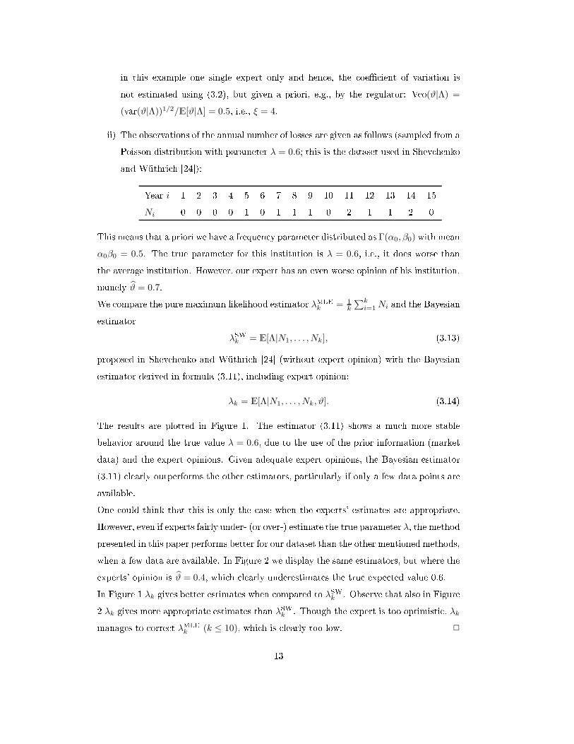
(var(ϑ|Λ))1/2/E[ϑ|Λ] = 0.5, i.e., ξ = 4.ii) The observations of the annual number of losses are given as follows (sampled from aPoisson distribution with parameter λ = 0.6; this is the dataset used in Shev henkoand Wüthri h [24℄):Year i 1 2 3 4 5 6 7 8 9 10 11 12 13 14 15Ni 0 0 0 0 1 0 1 1 1 0 2 1 1 2 0This means that a priori we have a frequen y parameter distributed as Γ(α0, β0) with mean

α0β0 = 0.5. The true parameter for this institution is λ = 0.6, i.e., it does worse thanthe average institution. However, our expert has an even worse opinion of his institution,namely ϑ̂ = 0.7.We ompare the pure maximum likelihood estimator λMLEk = 1k

∑ki=1 Ni and the Bayesianestimator

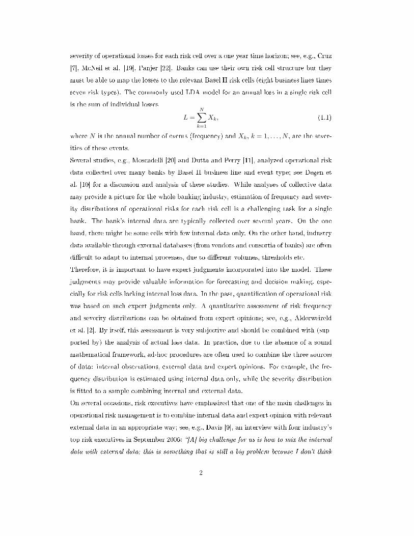
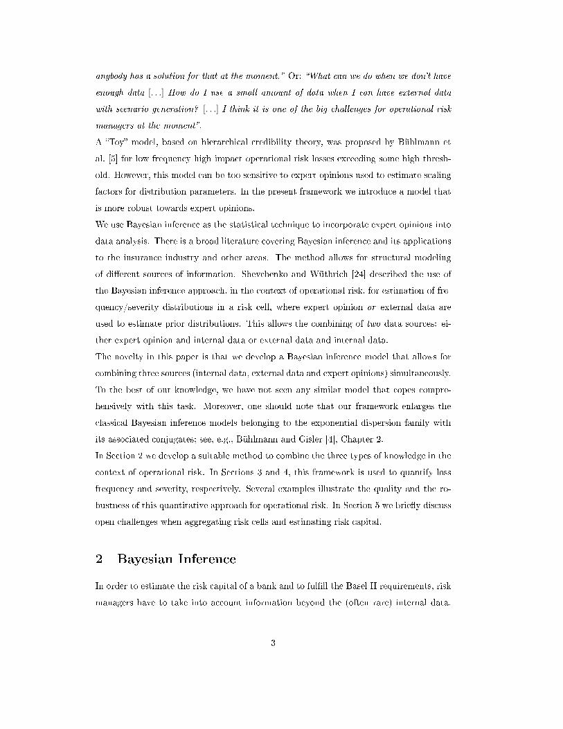
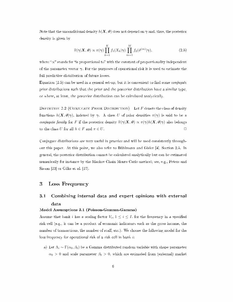
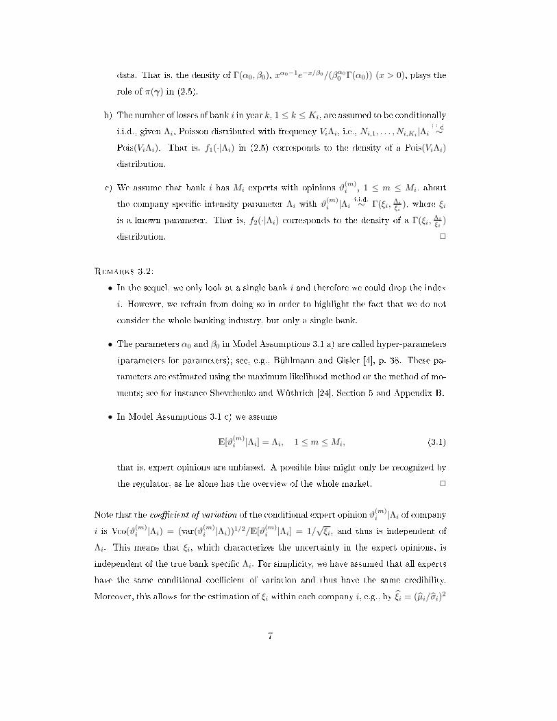
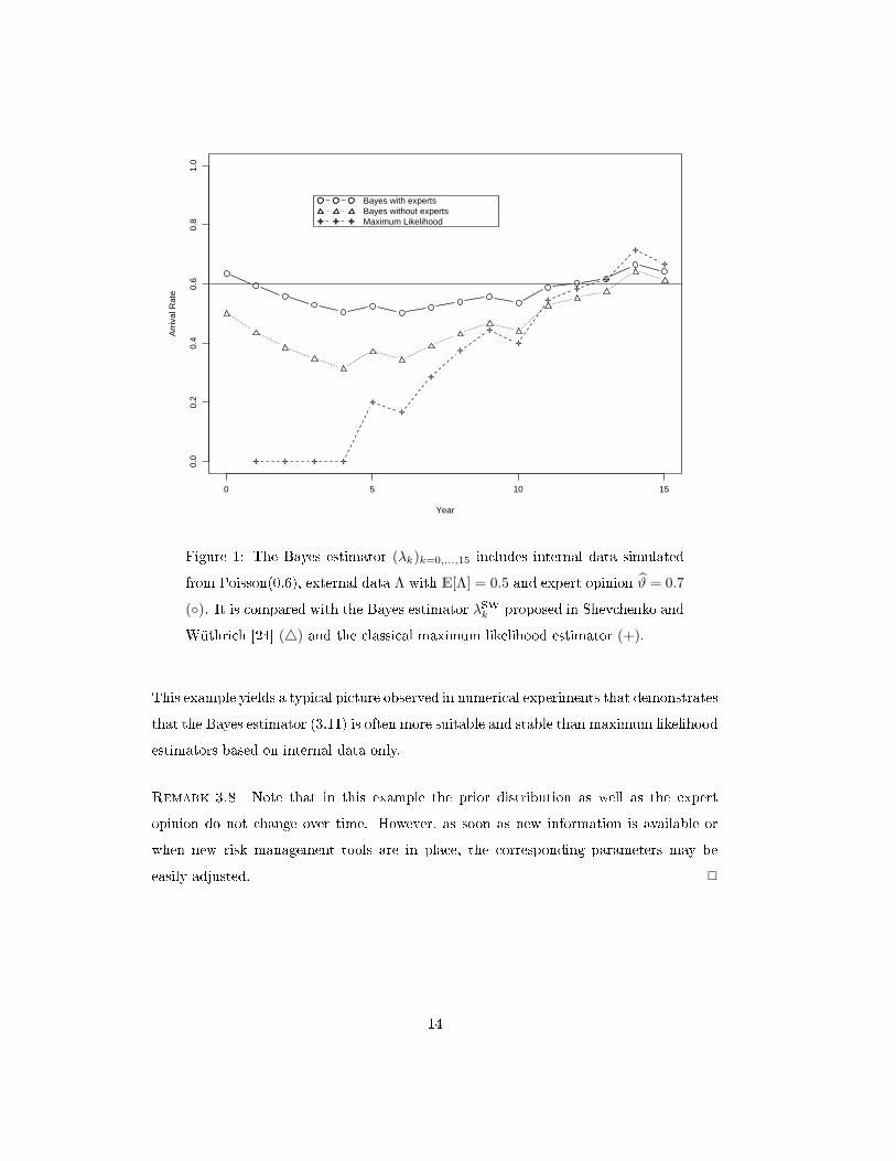
λSWk = E[Λ|N1, . . . , Nk], (3.13)proposed in Shev henko and Wüthri h [24℄ (without expert opinion) with the Bayesianestimator derived in formula (3.11), in luding expert opinion:λk = E[Λ|N1, . . . , Nk, ϑ]. (3.14)The results are plotted in Figure 1. The estimator (3.11) shows a mu h more stablebehavior around the true value λ = 0.6, due to the use of the prior information (marketdata) and the expert opinions. Given adequate expert opinions, the Bayesian estimator(3.11) learly outperforms the other estimators, parti ularly if only a few data points areavailable.One ould think that this is only the ase when the experts' estimates are appropriate.However, even if experts fairly under- (or over-) estimate the true parameter λ, the methodpresented in this paper performs better for our dataset than the other mentioned methods,when a few data are available. In Figure 2 we display the same estimators, but where theexperts' opinion is ϑ̂ = 0.4, whi h learly underestimates the true expe ted value 0.6.In Figure 1 λk gives better estimates when ompared to λSWk . Observe that also in Figure2 λk gives more appropriate estimates than λSWk . Though the expert is too optimisti , λkmanages to orre t λMLEk (k ≤ 10), whi h is learly too low. 213

Year

Arr

ival

Rat

e

0 5 10 15

0.0

0.2

0.4

0.6

0.8

1.0

✛ ✛ ✛ ✛

✛

✛

✛

✛

✛

✛

✛

✛

✛

✛

✛

✛ ✛ ✛✛ ✛ ✛

Bayes with expertsBayes without expertsMaximum Likelihood

Figure 1: The Bayes estimator (λk)k=0,...,15 in ludes internal data simulatedfrom Poisson(0.6), external data Λ with E[Λ] = 0.5 and expert opinion ϑ̂ = 0.7

(◦). It is ompared with the Bayes estimator λSWk proposed in Shev henko andWüthri h [24℄ (△) and the lassi al maximum likelihood estimator (+).This example yields a typi al pi ture observed in numeri al experiments that demonstratesthat the Bayes estimator (3.11) is often more suitable and stable than maximum likelihoodestimators based on internal data only.Remark 3.8 Note that in this example the prior distribution as well as the expertopinion do not hange over time. However, as soon as new information is available orwhen new risk management tools are in pla e, the orresponding parameters may beeasily adjusted. 2

14

Year

Arr

ival

Rat

e

0 5 10 15

0.0

0.2

0.4

0.6

0.8

1.0

✛ ✛ ✛ ✛

✛

✛

✛

✛

✛

✛

✛

✛

✛

✛

✛

✛ ✛ ✛✛ ✛ ✛

Bayes with expertsBayes without expertsMaximum Likelihood

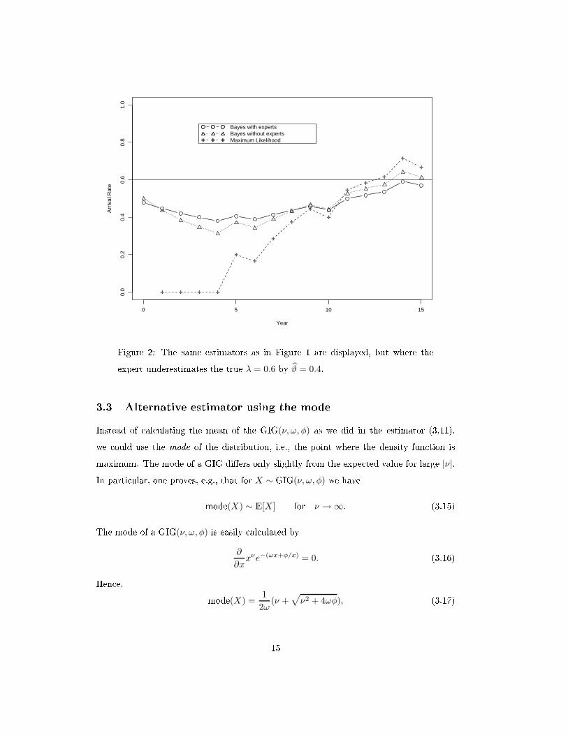
Figure 2: The same estimators as in Figure 1 are displayed, but where theexpert underestimates the true λ = 0.6 by ϑ̂ = 0.4.3.3 Alternative estimator using the modeInstead of al ulating the mean of the GIG(ν, ω, φ) as we did in the estimator (3.11),we ould use the mode of the distribution, i.e., the point where the density fun tion ismaximum. The mode of a GIG di�ers only slightly from the expe ted value for large |ν|.In parti ular, one proves, e.g., that for X ∼ GIG(ν, ω, φ) we havemode(X) ∼ E[X ] for ν → ∞. (3.15)The mode of a GIG(ν, ω, φ) is easily al ulated by∂

∂xxνe−(ωx+φ/x) = 0. (3.16)Hen e, mode(X) =

1

2ω(ν +

√ν2 + 4ωφ), (3.17)15

whi h gives us a good approximation to the mean for large ν. Thus, we havemode(Λi|Ni, ϑi) =ν

2ω

(1 + sign(ν)

√1 +

4ωφ

ν2

), (3.18)where ν, ω, and φ are given by equations (3.5). Due to 4ωφ

ν2 → 0 for Ki → ∞, Mi → ∞,Mi → 0 or ξ → 0, we approximate √1 + 2x ≈ 1 + x, x → 0, and hen emode(Λi|Ni, ϑi) ≈

ν

2ω1{ν≥0} +

φ

|ν| . (3.19)With (3.19) we again get the results from Theorem 3.6 in an elementary manner avoidingBessel fun tions.4 Loss SeveritiesIn the previous se tion we presented a method to quantify the operational risk loss fre-quen y. We now turn to quanti� ation of the severity distribution for operational risk.This is done in this se tion for di�erent types of subexponential models.4.1 Lognormal model (Model 1 for severities)Model Assumptions 4.1 (Lognormal-normal-normal)Let us assume the following severity model for operational risk of a risk ell in bank i,1 ≤ i ≤ I:a) Let ∆i ∼ N (µ0, σ0) be a normally distributed random variable with parameters

µ0, σ0, whi h are estimated from (external) market data, i.e., π(γ) in (2.5) is thedensity of N (µ0, σ0).b) The losses k = 1, . . . , Ki from institution i are assumed to be onditionally (on∆i) i.i.d. lognormally distributed: Xi,1, . . . , Xi,Ki

|∆ii.i.d.∼ LN(∆i, σi), where σi isassumed known. That is, f1(·|∆i) in (2.5) orresponds to the density of a LN(∆i, σi)distribution. ) We assume that bank i has Mi experts with opinions ϑ

(m)i , 1 ≤ m ≤ Mi, aboutthe parameter ∆i with ϑ

(m)i |∆i

i.i.d.∼ N (µi = ∆i, σ̃i = ξi), where ξi is a parameterestimated using expert opinion data. That is, f2(·|∆i) orresponds to the densityof a N (∆i, ξi) distribution. 216

Remarks 4.2:• For Mi ≥ 2, the parameter ξi is, e.g., estimated by the standard deviation of ϑ

(m)i :

ξi =

(1

Mi − 1

Mi∑

m=1

(ϑ(m)i − ϑi)

2

)1/2

. (4.1)• The hyper-parameters µ0 and σ0 are estimated from market data, e.g., by maximumlikelihood estimation or by the method of moments.• In pra ti e one often uses an ad ho estimate for σi, 1 ≤ i ≤ I, whi h usually isbased on expert opinion only. However one ould think of a Bayesian approa h for

σi, but then an analyti al formula for the posterior distribution in general does notexist. The posterior distribution needs then to be al ulated for example by theMarkov Chain Monte Carlo method; see again Peters and Sisson [23℄ or Gilks etal. [17℄. 2Under Model Assumption 4.1, the posterior density is given byπ̂∆i

(δi|Xi, ϑi) ∝ 1

σ0

√2π

exp

(− (δi − µ0)

2

2σ20

) Ki∏

k=1

1

σi

√2π

exp

(− (log Xi,k − δi)

2

2σ2i

)

Mi∏

m=1

1

σ̃i

√2π

exp

(− (ϑ

(m)i − δi)

2

2σ̃2i

)

∝ exp

[−(

(δi − µ0)2

2σ20

+

Ki∑

k=1

1

2σ2i

(log Xi,k − δi)2

+

Mi∑

m=1

1

2ξ2i

(ϑ(m)i − δi)

2

)]

∝ exp

[− (δi − µ̂)2

2σ̂2

], (4.2)with

σ̂2 =

(1

σ20

+Ki

σ2i

+Mi

ξ2i

)−1

, (4.3)andµ̂ = σ̂2 ·

(µ0

σ20

+1

σ2i

Ki∑

k=1

log Xi,k +1

ξ2i

Mi∑

m=1

ϑ(m)i

). (4.4)In summary we have the following theorem.Theorem 4.3Under Model Assumptions 4.1 and with the notation log Xi = 1

Ki

∑Ki

k=1 log Xi,k, the pos-terior distribution of ∆i, given loss information Xi and expert opinion ϑi, is a normal17

distribution N (µ̂, σ̂) withσ̂2 =

(1

σ20

+Ki

σ2i

+Mi

ξ2i

)−1

, (4.5)andµ̂ = E[∆i|Xi, ϑi] = ω1µ0 + ω2log Xi + ω3ϑi. (4.6)The redibility weights are ω1 = σ̂2/σ2

0, ω2 = σ̂2Ki/σ2i and ω3 = σ̂2Mi/ξ2

i .This theorem yields a natural interpretation of the onsidered model. The estimator µ̂ in(4.6) weights the internal and external data as well as the expert opinion in an appropriatemanner. Observe that under Model Assumptions 4.1 we an expli itly al ulate the meanof the posterior distribution. This is di�erent from the frequen y model in Se tion 3.That is, we have an exa t al ulation and for the interpretation of the terms we do notrely on an asymptoti theorem as in Theorem 3.6. However, interpretation of the terms isexa tly the same as in Theorem 3.6. The more redible the information, the higher is the redibility weight in (4.6). Hen e, again, this theorem shows that our model is appropriatefor ombining internal observations, relevant external data and expert opinions.4.2 Pareto model (Model 2 for severities)Model Assumptions 4.4 (Pareto-Gamma-Gamma)Let us assume the following severity model for a parti ular operational risk ell of banki, 1 ≤ i ≤ I:a) Let Γi ∼ Γ(α0, β0) be a Gamma distributed random variable with parameters α0, β0,whi h are estimated from (external) market data, i.e., π(γ) in (2.5) is the densityof a Γ(α0, β0) distribution.b) The losses k = 1, . . . , Ki from institution i are assumed to be onditionally (on Γi)i.i.d. Pareto distributed: Xi,1, . . . , Xi,Ki

|Γii.i.d.∼ Pareto(Γi, Li), where the threshold

Li ≥ 0 is assumed to be known and �xed. That is, f1(·|Γi) in (2.5) orresponds tothe density of a Pareto(Γi, Li) distribution. ) We assume that bank i has Mi experts with opinions ϑ(m)i , 1 ≤ m ≤ Mi, aboutthe parameter Γi with ϑ

(m)i |Γi

i.i.d.∼ Γ(αi = ξi, βi = Γi/ξi), where ξi is a parameterestimated using expert opinion data; see (3.2). That is, f2(·|Γi) orresponds to thedensity of a Γ(ξi, Γi/ξi) distribution. 218

Under Model Assumptions 4.4, the posterior density is given byπ̂Γi

(γi|Xi, ϑi) ∝ γα0−1i e−γi/β0

Ki∏

k=1

γi

Li

(Xi,k

Li

)−(γi+1) Mi∏

m=1

(ϑ(m)i /βi)

αi−1

βie−ϑ

(m)i

/βi

∝ γα0−1−Miξi+Ki

i exp

[−γi

(1

β0+

Ki∑

k=1

logXi,k

Li

)− 1

γiξiMiϑi

]. (4.7)Hen e, again, the posterior distribution is a GIG and it has the ni e property that theterm γi in the exponent in (4.7) is only a�e ted by the internal observations, whereas theterm 1/γi is driven by the expert opinions.Theorem 4.5Under Model Assumptions 4.4, the posterior density of Γi, given loss information Xi andexpert opinion ϑi, is given by

π̂Γi(γi|Xi, ϑi) =

(ω/φ)(ν+1)/2

2Kν+1(2√

ωφ)γν

i e−γiω−γ−1i

φ, (4.8)withν = α0 − 1 − Miξi + Ki,

ω =1

β0+

Ki∑

k=1

logXi,k

Li, (4.9)

φ = ξiMiϑi.It seems natural to generalize this result by substituting the prior Gamma distributionby a GIG as follows.Model Assumptions 4.6 (Pareto-Gamma-GIG)Let us assume the following severity model for a parti ular operational risk ell of banki, 1 ≤ i ≤ I:a) Let Γi ∼ GIG(ν0, ω0, φ0) be a generalized inverse Gaussian distributed randomvariable with parameters ν0, ω0, φ0, whi h are estimated from (external) marketdata, i.e., π(γ) in (2.5) is the density of a GIG(ν0, ω0, φ0) distribution.b) The losses k = 1, . . . , Ki from bank i are assumed to be onditionally (on Γi)i.i.d. Pareto distributed: Xi,1, . . . , Xi,Ki

|Γii.i.d.∼ Pareto(Γi, Li), where the threshold

Li ≥ 0 is assumed to be known and �xed. That is, f1(·|Γi) in (2.5) orresponds tothe density of a Pareto(Γi, Li) distribution.19

) We assume that bank i has Mi experts with opinions ϑ(m)i , 1 ≤ m ≤ Mi, aboutthe parameter Γi with ϑ

(m)i |Γi

i.i.d.∼ Γ(αi = ξi, βi = Γi/ξi), where ξi is a parameterestimated using expert opinion data. That is, f2(·|Γi) orresponds to the density ofa Γ(ξi, Γi/ξi) distribution. 2Under Model Assumptions 4.6, the a posteriori density π̂Γi(γi|Xi, ϑi) is given by (4.8)with

ν = ν0 − Miξi + Ki,

ω = ω0 +

Ki∑

k=1

logXi,k

Li, (4.10)

φ = φ0 + ξiMiϑi.Hen e, again, the posterior distribution is given by a GIG. Note that for φ0 = 0, the GIGis a Gamma distribution and hen e we are in the Pareto-Gamma-Gamma situation ofModel 4.4.The following theorem gives us a natural interpretation of the Bayesian estimatorE[Γi|Xi, ϑi] =

√φ

ωRν+1(2

√ωφ). (4.11)Denote the maximum likelihood estimator of the Pareto tail index Γi by

γMLEi =Ki∑Ki

k=1 logXi,k

Li

. (4.12)Then, ompletely analogous to Theorem 3.6 we obtain the following theorem.Theorem 4.7Under Model Assumptions 4.4 and 4.6, the following asymptoti relations hold P-almostsurely:a) Assume, given Γi = γi, Xi,ki.i.d.∼ Pareto(γi, Li) and ϑ

(m)i

i.i.d.∼ Γ(ξi, γi/ξi).For Ki → ∞ : E[Γi|Xi, ϑi] → E[Xi,k|Γi = γi]/Vi = γi.b) For V o(ϑ(m)i |Γi) → 0 : E[Γi|Xi, ϑi] → ϑ

(m)i , m = 1, . . . , Mi. ) Assume, given Γi = γi, Xi,k

i.i.d.∼ Pareto(γi, Li) and ϑ(m)i

i.i.d.∼ Γ(ξi, γi/ξi).For Mi → ∞ : E[Γi|Xi, ϑi] → E[ϑ(m)i |Γi = γi] = γi.d) For V o(ϑ(m)

i |Γi) → ∞, m = 1, . . . , Mi :

E[Γi|Xi, ϑi] →(1 − Kiβ0

γMLEi

+Kiβ0

)E[Γi] + Kiβ0

γMLEi

+Kiβ0γMLEi .20

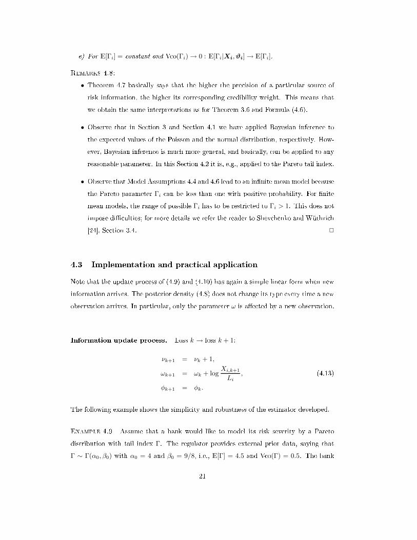
e) For E[Γi] = onstant and V o(Γi) → 0 : E[Γi|Xi, ϑi] → E[Γi].Remarks 4.8:• Theorem 4.7 basi ally says that the higher the pre ision of a parti ular sour e ofrisk information, the higher its orresponding redibility weight. This means thatwe obtain the same interpretations as for Theorem 3.6 and Formula (4.6).• Observe that in Se tion 3 and Se tion 4.1 we have applied Bayesian inferen e tothe expe ted values of the Poisson and the normal distribution, respe tively. How-ever, Bayesian inferen e is mu h more general, and basi ally, an be applied to anyreasonable parameter. In this Se tion 4.2 it is, e.g., applied to the Pareto tail index.• Observe that Model Assumptions 4.4 and 4.6 lead to an in�nite mean model be ausethe Pareto parameter Γi an be less than one with positive probability. For �nitemean models, the range of possible Γi has to be restri ted to Γi > 1. This does notimpose di� ulties; for more details we refer the reader to Shev henko and Wüthri h[24℄, Se tion 3.4. 24.3 Implementation and pra ti al appli ationNote that the update pro ess of (4.9) and (4.10) has again a simple linear form when newinformation arrives. The posterior density (4.8) does not hange its type every time a newobservation arrives. In parti ular, only the parameter ω is a�e ted by a new observation.Information update pro ess. Loss k → loss k + 1:

νk+1 = νk + 1,

ωk+1 = ωk + logXi,k+1

Li, (4.13)

φk+1 = φk.The following example shows the simpli ity and robustness of the estimator developed.Example 4.9 Assume that a bank would like to model its risk severity by a Paretodistribution with tail index Γ. The regulator provides external prior data, saying thatΓ ∼ Γ(α0, β0) with α0 = 4 and β0 = 9/8, i.e., E[Γ] = 4.5 and V o(Γ) = 0.5. The bank21

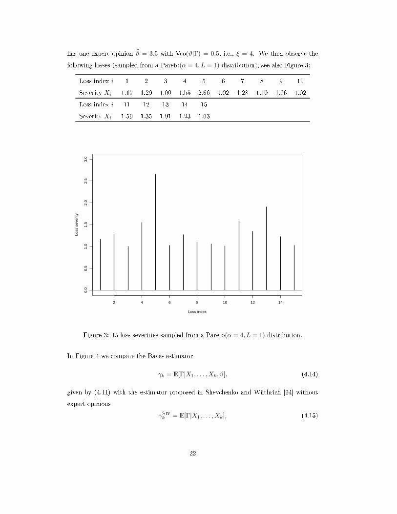
has one expert opinion ϑ̂ = 3.5 with V o(ϑ|Γ) = 0.5, i.e., ξ = 4. We then observe thefollowing losses (sampled from a Pareto(α = 4, L = 1) distribution); see also Figure 3:Loss index i 1 2 3 4 5 6 7 8 9 10Severity Xi 1.17 1.29 1.00 1.55 2.66 1.02 1.28 1.10 1.06 1.02Loss index i 11 12 13 14 15Severity Xi 1.59 1.35 1.91 1.23 1.03

Loss index

Loss

sev

erity

2 4 6 8 10 12 14

0.0

0.5

1.0

1.5

2.0

2.5

3.0

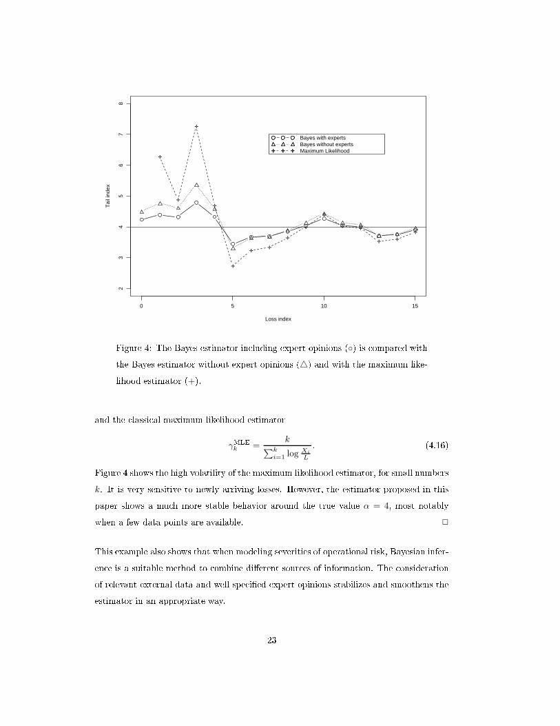
Figure 3: 15 loss severities sampled from a Pareto(α = 4, L = 1) distribution.In Figure 4 we ompare the Bayes estimatorγk = E[Γ|X1, . . . , Xk, ϑ], (4.14)given by (4.11) with the estimator proposed in Shev henko and Wüthri h [24℄ withoutexpert opinionsγSWk = E[Γ|X1, . . . , Xk], (4.15)22

Loss index

Tai

l ind

ex

0 5 10 15

23

45

67

8

✛

✛

✛

✛

✛

✛✛

✛

✛

✛

✛ ✛

✛ ✛

✛

✛ ✛ ✛✛ ✛ ✛

Bayes with expertsBayes without expertsMaximum Likelihood

Figure 4: The Bayes estimator in luding expert opinions (◦) is ompared withthe Bayes estimator without expert opinions (△) and with the maximum like-lihood estimator (+).and the lassi al maximum likelihood estimatorγMLEk =

k∑k

i=1 log Xi

L

. (4.16)Figure 4 shows the high volatility of the maximum likelihood estimator, for small numbersk. It is very sensitive to newly arriving losses. However, the estimator proposed in thispaper shows a mu h more stable behavior around the true value α = 4, most notablywhen a few data points are available. 2This example also shows that when modeling severities of operational risk, Bayesian infer-en e is a suitable method to ombine di�erent sour es of information. The onsiderationof relevant external data and well-spe i�ed expert opinions stabilizes and smoothens theestimator in an appropriate way. 23

5 Total loss distribution and risk apital estimatesIn the pre eding se tions we have des ribed how the parameters of the distributions areestimated. A ording to the Basel II requirements (see BIS [6℄) the �nal bank apitalshould be al ulated as a sum of the risk measures in the risk ells if the bank's model annot a ount for orrelations between risks a urately. If this is the ase, then one needsto al ulate VaR for ea h risk ell separately and sum VaRs over risk ells to estimatethe total bank apital. Adding quantiles over the risk ells to �nd the quantile of thetotal loss distribution is sometimes too onservative. It is equivalent to the assumptionof perfe t dependen e between risks.The al ulation of VaR (taking into a ount parameter un ertainty) for ea h risk ell an,in view of the previous se tions, easily be done using a simulation approa h des ribedin Shev henko and Wüthri h [24℄, Se tion 6. Simulation pro edures for independent risk ells and in the ase of dependen e between risks are also des ribed in Shev henko andWüthri h [24℄ and thus we refrain from ommenting further on this issue.However, reasonable aggregation is still an open hallenging problem that needs furtherinvestigation. The hoi e of appropriate dependen e stru tures is ru ial and determinesthe amount of diversi� ation. In the general ase, when no information about the depen-den e stru ture is available, Embre hts and Pu etti [15℄ work out bounds for aggregatedoperational risk apital; for further issues regarding aggregation we would like to refer toEmbre hts et al. [14℄.6 Con lusionIn this paper we propose a novel approa h that allows for ombining three data sour es:internal data, external data and expert opinions. The approa h is based on the Bayesianinferen e method. It is applied to the quanti� ation of the frequen y and severity distri-butions in operational risk, where there is a strong need for su h a method to meet theBasel II regulatory requirements.The method is based on spe ifying prior distributions for the parameters of the frequen yand severity distributions using industry data. Then, the prior distributions are weightedby the a tual observations and expert opinions from the bank to estimate the posteriordistributions of the model parameters. These are used to estimate the annual loss distri-bution for the next reporting year. Estimation of low frequen y risks using this method24

has several appealing features su h as: stable estimators, simple al ulations (in the aseof onjugate priors), and the ability to take expert opinions and industry data into a - ount. This method also allows for al ulation of VaR with parameter un ertainty takeninto a ount.For onvenien e we have assumed that expert opinions are i.i.d. but all formulas an easilybe generalized to the ase of expert opinions modeled by di�erent distributions.It would be ideal if the industry risk pro�les (prior distributions for frequen y and severityparameters in risk ells) are al ulated and provided by the regulators to ensure onsis-ten y a ross the banks. Unfortunately this may not be realisti at the moment. Banksmight thus estimate the industry risk pro�les using industry data available through ex-ternal databases from vendors and onsortia of banks. The data quality, reporting andsurvival biases in external databases are the issues that should be onsidered in pra ti ebut go beyond the purposes of this paper.The approa h des ribed is not too ompli ated and is well suited for operational riskquanti� ation. It has a simple stru ture, whi h is bene� ial for pra ti al use and anengage the bank risk managers, statisti ians and regulators in produ tive model develop-ment and risk assessment. The model provides a framework that an be developed furtherby onsidering other distribution types, dependen ies between risks and dependen e ontime.One of the features of the des ribed method is that the varian e of the posterior distri-bution π̂(γ|·) will onverge to zero for a large number of observations. That is, the truevalues of the risk parameters will be known exa tly. However, there are many fa tors (forexample, politi al, e onomi al, legal, et .) hanging in time that will not permit for thepre ise knowledge of the risk parameters. One an model this by limiting the varian eof the posterior distribution by some lower levels (say, e.g., 5%). This has been done inmany solven y approa hes for the insuran e industry; see, e.g., the Swiss Solven y Test,FOPI [16℄, formulas (25)-(26).Although the main impetus motivation for the present paper is an urgent need from op-erational risk pra titioners, the proposed method is also useful in other areas (su h as redit risk, insuran e, environmental risk, e ology et .) where, mainly due to la k of inter-nal observations, a ombination of internal data with external data and expert opinionsis required. 25

A Generating realizations from a GIG random variableFor pra ti al purposes it is required to generate realizations of a random variable X ∼GIG(ω, φ, ν) with ω, φ > 0. Observe that we need to onstru t a spe ial algorithm sin ewe an not invert the distribution fun tion analyti ally. The following algorithm an befound in Dagpunar [8℄; see also M Neil et al. [19℄:Algorithm A.1 (Generalized inverse Gaussian)1. α =√

ω/φ; β = 2√

ωφ,m = 1

β

(ν +

√ν2 + β2

),g(y) = 1

2βy3 − y2(12βm + ν + 2) + y(νm − β

2 ) + 12βm.2. Set y0 = m,While g(y0) ≤ 0 do y0 = 2y0,

y+: root of g in the interval (m, y0),y−: root of g in the interval (0, m).3. a = (y+ − m)

(y+

m

)ν/2exp

(−β

4 (y+ + 1y+

− m − 1m)),

b = (y− − m)(y

−

m

)ν/2exp

(−β

4 (y− + 1y−

− m − 1m )),

c = −β4

(m + 1

m

)+ ν

2 log(m).4. Repeat U, V ∼ Unif(0, 1), Y = m + aUV + b 1−V

U ,until Y > 0 and − log U ≥ − ν2 log Y + 1

4β(Y + 1Y ) + c,Then X = Y

α is GIG(ω, φ, ν); see Dagpunar [8℄.To generate a sequen e of n realizations from a GIG random variable, step 4 is repeatedn times. 2B Asymptoti results for modi�ed Bessel fun tionsLet Kγ(z) denote the modi�ed Bessel fun tion of the third kind as de�ned in (3.6).Lemma B.1 With notation (3.10), we have the following asymptoti relation for ν →∞, for all a, b > 0:

Rbν(a√

ν) ∼ 2b√

ν

a. (B.1)

26

Proof: From Abramowitz and Stegun [1℄, Paragraph 9.7.8 and Olver [21℄, Chapter 4,we may dedu e for large ν and z ≥ 0

Kν(νz) =

√π

2ν

exp(−ν√

1 + z2)

(1 + z2)1/4

(z

1 +√

1 + z2

)−ν

(1 + ε(ν, z)) , (B.2)where the error term ε(ν, z) is bounded by|ε(ν, z)| ≤ 1

ν − ν0

∫ 1/√

1+z2

0

|u′1(s)|ds, (B.3)with ν0 = 1

6√

5+ 1

12 and u1(s) = (3s−5s3)/24; see Abramowitz and Stegun [1℄ for details.In (B.2) we repla e ν by bν and z by z1 = a/√

ν. The error term ε(bν, a/√

ν) in (B.2) isthen vanishing for ν → ∞, be ause the right-hand side of (B.3) tends to 0. Analogously,we repla e ν by bν+1 and z by z2 = a√

ν/(bν+1) and observe that ε(bν+1, a√

ν/(bν+1))tends to 0. Thus, (B.2) gives us asymptoti expressions for Kbν(a√

ν) and Kbν+1(a√

ν).Straightforward al ulations then yieldRbν(a

√ν) =

Kbν+1(a√

ν)

Kbν(a√

ν)∼ 2

z2∼ 2b

√ν

a, ν → ∞. (B.4)This ompletes the proof. 2C Proof of Theorem 3.6Proof: With (3.11) the proof of this theorem is straightforward, using Lemma B.1 inAppendix B. The following statements hold P-almost surely.a) √ φ

ω Rν+1(2√

ωφ) ∼√

φω RKiNi

(2√

ViKiφ) ∼√

Ki

ViωNi ∼ E[Ni,k|Λi]/Vi.b, ) √ φ

ω Rν+1(2√

ωφ) ∼√

φω R−Miξi

(2√

ωξiMiϑi) ∼√

φω

1

RMiξi(2√

ωξiMiϑi)

∼√

φϑi

ξiMi= ϑi = ϑ

(m)i , m = 1, . . . , Mi.d) If ξ = 0, we are in the Gamma ase Γ(α, β) with α = α0 + KiN i and β =

β0/(ViKiβ0 + 1). Hen e,E[Λi|Ni, ϑi] = αβ = 1

ViKiβ0+1E[Λi] +(1 − 1

ViKiβ0+1

)N i/Vi.e) √ φ

ω Rν+1(2√

ωφ) ∼√

φE[Λi]α0

Rα0(2√

α0φE[Λi]

) ∼ E[Λi]. 2

27

A knowledgmentsThe authors would like to thank Isaa Meilijson for several fruitful dis ussions and PaulEmbre hts for his useful omments.Referen es[1℄ Abramowitz, M. and Stegun, I. A. (1965) Handbook of Mathemati al Fun tions .Dover Publi ations, New York.[2℄ Alderweireld, T., Gar ia, J. and Léonard, L. (2006) A pra ti al operational risks enario analysis quanti� ation. Risk Magazine 19(2), 93�95.[3℄ Atkinson, A. C. (1982) The simulation of generalized inverse Gaussian and hyperboli random variables. SIAM Journal of S ienti� and Statisti al Computation 3, 502�515.[4℄ Bühlmann, H. and Gisler, A. (2005) A Course in Credibility Theory and its Appli a-tions . Springer, Berlin.[5℄ Bühlmann, H., Shev henko, P. V. and Wüthri h, M. V. (2007) A �toy� model foroperational risk quanti� ation using redibility theory. Journal of Operational Risk2(1), 3�19.[6℄ BIS (2005) Basel II: International Convergen e of Capital Measurement and Cap-ital Standards: a revised framework. Bank for International Settlements (BIS),www.bis.org.[7℄ Cruz, M. G. (2002) Modeling, Measuring and Hedging Operational Risk . Wiley,Chi hester.[8℄ Dagpunar, J. S. (1989) An easily implemented generalised inverse Gaussian generator.Communi ations in Statisti s, Simulation and Computation 18, 703�710.[9℄ Davis, E. (2006) Theory vs Reality. OpRisk and Complian e. 1 September 2006,www.opriskand omplian e. om/publi /showPage.html?page=345305.[10℄ Degen, M., Embre hts, P. and Lambrigger, D. D. (2007) The quantitative modelingof operational risk: between g-and-h and EVT. ASTIN Bulletin, to appear.28

[11℄ Dutta, K. and Perry, J. (2006) A tale of tails: an empiri al analysis of loss distribu-tion models for estimating operational risk apital. Federal Reserve Bank of Boston,Working Paper No 06-13.[12℄ Embre hts, P. (1983) A property of the generalized inverse Gaussian distributionwith some appli ations. Journal of Applied Probability 20, 537�544.[13℄ Embre hts, P., Klüppelberg, C. and Mikos h, T. (1997) Modelling Extremal Eventsfor Insuran e and Finan e. Springer, Berlin.[14℄ Embre hts, P., Ne²lehová, J. and Wüthri h, M. V. (2007) Additivity properties forValue-at-Risk under ar himedean dependen e and heavy-tailedness. Preprint, ETHZuri h.[15℄ Embre hts, P. and Pu etti, G. (2006) Aggregating risk apital, with an appli ationto operational risk. The Geneva Risk and Insuran e Review 31(2), 71�90.[16℄ FOPI (2006) Swiss Solven y Test, Te hni al Do ument. Federal O� e of PrivateInsuran e, Bern. www.bpv.admin. h/themen/00506/00552.[17℄ Gilks, W. R., Ri hardson, S. and Spiegelhalter, D. J. (1996) Markov Chain MonteCarlo in pra ti e. Chapman & Hall, London.[18℄ Jørgensen, B. (1982) Statisti al Properties of the Generalized Inverse Gaussian Dis-tribution. Springer, New York.[19℄ M Neil, A. J., Frey, R. and Embre hts, P. (2005) Quantitative Risk Management:Con epts, Te hniques and Tools . Prin eton University Press, Prin eton.[20℄ Mos adelli, M. (2004) The modelling of operational risk: experien es with the anal-ysis of the data olle ted by the Basel Committee. Bank of Italy, Working Paper No517.[21℄ Olver, F. W. J. (1962) Mathemati al Tables, vol. 6, Tables for Bessel fun tions ofmoderate or large orders . National Physi al Laboratory. Her Majesty's StationeryO� e, London.[22℄ Panjer, H. H. (2006) Operational Risks: Modeling Analyti s . Wiley, New York.[23℄ Peters, G. W. and Sisson, S. A. (2006) Bayesian inferen e, Monte Carlo samplingand operational risk. Journal of Operational Risk 1(3), 27�50.29

[24℄ Shev henko, P. V. andWüthri h, M. V. (2006) The stru tural modeling of operationalrisk via Bayesian inferen e: ombining loss data with expert opinions. Journal ofOperational Risk 1(3), 3�26.

30