The QALY model wich came in from a general population survey: roughly multiplicative, broadly nonlinear and sometimes contex-dependt

DOCUMENTO DE TRABAJO. E2009/ 04

The QALY model which came in from a general population survey,roughly multiplicative, broadly nonlinear and sometimes context-dependent

JOSE Mª ABELLÁN-PERPIÑÁNJORGE EDUARDO MARTÍNEZ PÉREZFERNANDO IGNACIO SÁNCHEZ MARTÍNEZILDEFONSO MÉNDEZ MARTÍNEZ

Cen

tro

de

Est

ud

ios

An

dal

uce

s El Centro de Estudios Andaluces es una entidad de carácter científico y cultural, sin ánimo de lucro, adscrita a la Consejería de la Presidencia de la Junta de Andalucía. El objetivo esencial de esta institución es fomentar cuantitativa y cualitativamente una línea de estudios e investigaciones científicas que contribuyan a un más preciso y detallado conocimiento de Andalucía, y difundir sus resultados a través de varias líneas estratégicas. El Centro de Estudios Andaluces desea generar un marco estable de relaciones con la comunidad científica e intelectual y con movimientos culturales en Andalucía desde el que crear verdaderos canales de comunicación para dar cobertura a las inquietudes intelectuales y culturales. Las opiniones publicadas por los autores en esta colección son de su exclusiva responsabilidad © 2009. Fundación Centro de Estudios Andaluces. Consejería de Presidencia. Junta de Andalucía © Autores Depósito Legal: DL SE 2681-2009 Ejemplar gratuito. Prohibida su venta.

Cen

tro

de

Est

ud

ios

An

dal

uce

s

E2009/04 The QALY model wich came in from a general population survey:

roughly multiplicative, broadly nonlinear and sometimes contex-dependent

José Mª Abellán -Perpiñán* Universidad de Murcia

Jorge Eduardo Martínez Pérez

Universidad de Murcia

Fernando-Ignacio Sánchez-Martínez Universidad de Murcia

Ildefonso Mendez-Martínez

Universidad de Murcia

Este trabajo aplica un método, propuesto inicialmente por Miyamoto (2000), para ajustar los pesos de calidad de vida (o utilidades de los estados de salud) en función de la curvatura de la función de utilidad del tiempo de vida. El procedimiento de ajuste aplicado es robusto ante fenómenos como la propagación del error y el sesgo ocasionado por la transformación de la probabilidad. Los parámetros de curvatura estimados fueron, por lo general, consistentes con la evidencia empírica precedente. Asimismo, el presente estudio también recoge varios contrastes de axiomas clave para el modelo AVAC (Año de Vida Ajustado por la Calidad), válidos tanto para el paradigma de la utilidad esperada como para el paradigma de la utilidad dependiente del orden. Los resultados alcanzados, merced a una encuesta realizada a una gran muestra de población general, sugieren que las preferencias “medianas” de dicha muestra pueden aproximarse razonablemente bien mediante un modelo AVAC multiplicativo, dotado de una función de utilidad potencial del tiempo de vida. Por último, para un número relativamente considerable de estados de salud, hallamos evidencia contraria a la práctica habitual de transferir las utilidades de los estados de salud del contexto de decisión en el que fueron estimadas (p.ej. un contexto de certidumbre) a otro contexto diferente (p.ej. un contexto de incertidumbre). Acknowledgements: this working paper was made possible through a research grant (PRY103/08) from the Fundación Centro de Estudios Andaluces * Autor correspondencia:[email protected]

Cen

tro

de

Est

ud

ios

An

dal

uce

s

Abstract

This paper applies a method, first proposed by Miyamoto (2000), to adjust health state

utilities accounting for curvature of the utility function of life duration. Such a method

is not susceptible to error propagation and avoids biases due to probability weighting.

Group estimates obtained with the new adjustment method were, in general, consistent

with previous evidence. Several axiomatic tests of the QALY model under both

expected utility and rank-dependent utility were also performed. According to the

results obtained from a large general population survey, it seems that a multiplicative

QALY model with a power utility function for life duration may be a reasonable

approximation to individual true preferences. Finally, we also found that the common

practice of freely transferring health state utilities across riskless and risky contexts may

be wrong for a significant number of conditions.

Keywords: biases, expected utility, rank-dependent utility, time trade-off, value lottery equivalence

2

Cen

tro

de

Est

ud

ios

An

dal

uce

sIntroduction

This paper is concerned with some biases that may distort both health state utility

measurements and their use in subsequent applications. Throughout this manuscript a

bias is intended to be as any deviation from the individual true preference. We think that

the goal of elicitation methods is to discover such a true (although eventually hidden)

preference (Plott, 1996). Otherwise applications based on health state utilities, such as

cost-utility analyses, might lead to undesirable decisions. Imagine that an economic

evaluation agency prioritizes a health programme instead of other because the former

has a cost-utility ratio lower than the latter. Assume that the utilities used as inputs to

calculate the ratio did not reflect the societal preferences. The result would be clearly

inefficient. The National Health Service would give priority to an intervention which is

less preferred by the citizens than other. For this reason it is very important to identify

and correct biases.

Within the realm of health state utility measurement, sources of biases are

numerous. One main source is that expected utility does not characterize preferences

very well. Violations of expected utility provoke that potentially all elicitation methods

under risk may lead to biased utilities. Indeed, although the deficiencies of the standard

gamble (SG) method have deserved special attention (Llewellyn-Thomas et al., 1982;

Bleichrodt, 2001; Oliver, 2003), a similar lack of descriptive validity has been also

found for other procedures under risk (Oliver, 2005; Bleichrodt et al., 2007). The key

point in all cases is that biases arise as far as it is assumed that the methods can be

evaluated under expected utility. However, there is substantial evidence to show that

individuals deviate from expected utility. For example, people seem to process

probabilities in a non-linear way. This bias is typically called ‘probability weighting’ by

both rank-dependent utility theory (Quiggin, 1982) and prospect theory (Tversky and

3

Cen

tro

de

Est

ud

ios

An

dal

uce

sKahneman, 1992), currently two of the most popular descriptive alternatives to expected

utility. Wakker and Sttigelbout (1995) and Bleichrodt (2002) showed that the SG may

lead to utilities biased upwards if people underweight probabilities. Bleichrodt et al.

(2007) confirmed these previous theoretical analyses, concluding that other methods

under risk might also be affected by probability weighting.

On the other hand, elicitation methods under certainty such as the time trade-off

(TTO) do not suffer from probability weighting. Other biases, however, may affect

them. The way in which TTO utilities are commonly calculated assumes that the utility

function for life duration is linear. There is nevertheless a significant body of evidence

showing that the utility function for life years is concave rather than linear (McNeil et

al., 1978; Sttiggelbout et al., 1994; Stalmeier et al., 1996; Martin et al., 2000). This

evidence would imply that TTO utilities could be biased downwards (Bleichrodt, 2002).

The bias caused by utility curvature does not affect the SG because this method

imposes no restriction on the utility function for duration. Bleichrodt et al. (2007),

however, showed that there are other methods under risk whose utilities are affected by

utility curvature in a similar way as the TTO. Specifically, the method they called ‘value

lottery equivalence’ (VLE) resembles the idea of a TTO framed in terms of risk. As a

result of this similarity, VLE utility is in fact the same as that measured by the TTO.

Therefore, utility curvature may distort utilities measured through the VLE, an

elicitation procedure under risk, in the same way as the TTO method does, a technique

framed under certainty. This distortion is produced because the quality adjusted life year

(QALY) model is assumed. Such a model requires that the utility of living for a period

of time in a health state followed by death can be computed as the product of the time

period in the health state and the utility of that state. Thus, the utility function for life

4

Cen

tro

de

Est

ud

ios

An

dal

uce

sduration is assumed to be linear. Hereinafter, when we refer to the QALY model we

will mean the linear model.

In this paper we apply a new method to adjust TTO and VLE utilities by taken

into account that utility function for life duration is not linear and that individual

preferences deviate from expected utility. The procedure was proposed by Miyamoto

(2000), and to the best of our knowledge, it has not been used in an empirical study up

to now. This method offers a balance between the advantages of parametric and

nonparametric measurements of the utility function of life duration, in a similar way as

recently Abdellaoui et al. (2008) have measured utility for money outcomes under

prospect theory. In both cases elicitations are performed by using a small number of

certainty equivalents (CEs). We only require 6 elicitations per health state. In this point

the method is very similar to the common procedure used to fit the degree of curvature

of the utility function of life years which is also based on CEs (Miyamoto and Eraker,

1985; Stiggelbout et al., 1994; van Osch et al., 2004). One key difference with respect

to those studies, is that in our case the CEs are not linked and, hence, not prone to error

propagation. Finally, other critical distinction is that we can fully evaluate the CEs

under rank-dependent utility without imposing assumptions on the shape of the

probability weighting function.

The two health state utility measurement methods used in this study, the TTO

and the VLE, allow us to provide more insight in the question whether utilities derived

from one context in which health outcomes are taken for certain (intertemporal trade-

offs) can be freely applied to a decision context under risk. This is indeed a common

practice in both cost-utility and medical decision analysis. As both the TTO and the

VLE should lead to the same utility, any difference we observe should be attributed to

the different framing of decisions. There is some previous evidence supporting the idea

5

Cen

tro

de

Est

ud

ios

An

dal

uce

sof a unified concept of utility (Wakker, 1994), both for health outcomes (Attema et al.,

2007; Stalmeier and Bezembider, 1999) and for money outcomes (Abdellaoui et al.,

2007). Notwithstanding, recent evidence (Abellan et al., 2007) suggests caution against

routinely assuming that transferability of the same utility across different contexts is

justified.

In addition to the new adjustment method presented in this paper, we also report

the results from various nonparametric tests of the QALY model. Although previous

evidence is contrary to the assumption of linear utility function of life duration, most

analyses were based on expected utility. Until now, there are only two tests performed

under non-expected utility. Bleichrodt and Pinto (2005) rejected the QALY model

under a model consistent with rank-dependent utility, whereas Doctor et al. (2004)

found support for the QALY model using a test also valid under prospect theory.

In this paper we test a very general axiom due to Miyamoto (1999), valid under

rank-dependent utility, which is necessary for the linear QALY model. One contribution

of this paper is that, using a very simple axiomatic condition, we confirm the

conclusions previously reached by Bleichrodt and Pinto (2005) . In addition to that, we

find strong nonparametric evidence consistent with a power utility function for life

years. This is a relevant result since evidence from previous axiomatic tests was

negative (Miyamoto and Eraker, 1989), and parametric estimations often do not find

differences in goodness of fit between power and exponential models (Bleichrodt and

Pinto, 2005; Abdellaoui et al., 2007). Finally, we also test a more general QALY model,

in which utility curvature is allowed to change as the severity of the health status varies.

A potential weakness of most previous tests of the QALY model is that

empirical studies tipycally employed a small sample-size (around fifty people) and only

a few health states (two or three at best). Therefore conclusions have to be specially

6

Cen

tro

de

Est

ud

ios

An

dal

uce

scautious. For example, Attema and Brouwer (2009) have recently provided further

evidence that respondents indeed do not have a linear utility function for life duration.

In fact, Attema and Brouwer derived the degree of utility curvature. However, because

of only one particular health state (back pain) was considered, Attema and Brouwer

recognize (p. 241) that “cannot exclude the possibility that different utility of life

duration functions exist for different health states”. Consequently, new tests performed

with wider samples and health states sets would be highly advisable in order to provide

more robust insight on the validity of the QALY model.

As an attempt to overcome potential drawbacks such as those we have just

described, all our tests were performed for a large sample (N=656) and variety of health

states (18 EQ-5D states). Moreover, unlike the common practice of testing axioms in

‘controlled’ environments, we surveyed general population. We hope that this large

data-base provide more firm insight in the topics we have outlined above.

The structure of the paper is as follows. Section 2 provides background. Section

3 describes the elicitation methods and the tests addressed in this paper. Section 4

describes the survey. Section 5 shows the main results obtained. Section 6 concludes.

2. Background

2.1 Notation and structural assumptions

Let (Q1, T1; Q2, T2; …;Qn, Tn) denote a typical health profile that yields health state Qt

for duration Tt. A health profile is reduced to a chronic health outcome if Q1 = Q2 = …

= Qn. We will denote a chronic health outcome as (Q, T), where Q denotes health state

and T life duration, followed by death. The durations T belong to an interval Φ= [0, M],

where M is the maximum life duration, and Ω stands for the set of health states. We also

consider binary prospects denoted by ((Q1, T1), p; (Q2, T2)), yielding outcome (Q1, T1)

7

Cen

tro

de

Est

ud

ios

An

dal

uce

swith probability p and outcome (Q2, T2) with probability 1-p. If p = 1 or p = 0 the

prospect is riskless, otherwise it is risky.

By f we denote the preference relation meaning “as least as good as” defined

over the set of prospects l. Strict preferences are denoted by f and indifferences by ~.

Preferences over outcomes coincide with preferences over riskless prospects.

Throughout the paper we will assume that risky prospects are rank-ordered. That

is, when we write ((Q1, T1), p; (Q2, T2)) we assume that (Q1, T1) f (Q2, T2). This

assumption is not a restriction because each prospect can be written in this form by re-

ordering the outcomes.

Let Ω+ be the set of better-than-death health states. A health state Q1 is better-

than-death if (Q1, T1) f (Q1, T2) for every Φ∈21 ,TT such that T1 > T2. Given a better-

than-death state, preference is an increasing function of duration (i.e., people prefer

more life years to less). Let Ω- be the set of worse-than-death health states. A health

state Q2 is worse-than-death if (Q2, T1) f (Q2, T2) for every Φ∈21 ,TT such that T1 < T2.

Given a worse-than-death state, preference is a decreasing function of duration (i.e.,

people prefer less life years to more).

2.2 Expected utility and rank-dependent utility

Expected utility holds if the utility of any prospect ((Q1, T1), p; (Q2, T2)) can be

written as

pU(Q1, T1) + (1-p)U(Q2, T2), (1)

where U is a real-valued function over outcomes which is unique up to positive affine

transformations.

8

Cen

tro

de

Est

ud

ios

An

dal

uce

sRank-dependent utility generalizes expected utility by allowing probability

weighting. Rank-dependent utility holds if the utility of any prospect ((Q1, T1), p; (Q2,

T2)) can be written as

( ) ( ) ( )( ) ( )2211 ,1, TQUpwTQUpw −+ , (2)

where U is a real-valued function over outcomes which is unique up to positive affine

transformations and w is a probability weighting function which is increasing and

satisfies w(0) = 0 and w(1) = 1.

Empirical evidence (Gonzalez and Wu, 1999; Abdellaoui, 2000; Bleichrodt and

Pinto, 2000) suggests that the probability weighting function is typically ‘inverse S-

shaped’ with a point of inflection, where the function changes from overweighting

probabilities, i.e., w(p) > p, to underweighting probabilities, i.e., w(p) < p, lying around

0.35. Expected utility is the special case of rank-dependent utility when w(p) = p.

2.3 QALY models

Under the QALY model the utility of chronic health outcomes in expected

utility, rank-dependent utility, and prospect theory is the following

( ) ( )TQHTQU =, , (3)

where H is the utility of the health state. According to the usual scaling H(FH) = 1 and

U(Death) = 0.

The non-linear QALY model generalizes the QALY model by allowing utility

curvature for life duration. The non-linear QALY model may be written in two different

forms, either multiplicative or nonmultiplicative. Under the multiplicative QALY model

U(Q, T)= H(Q)L(T), where L is the utility function of life duration. This model requires

that L is independent on the health state. On the contrary, the non-multiplicative QALY

model generalizes the multiplicative one by allowing utility curvature to vary as a

9

Cen

tro

de

Est

ud

ios

An

dal

uce

sfunction of health state, i.e., U(Q, T) = H(Q)L(TQ), where TQ denotes the dependence of

T from Q.

We will also consider two possible functional forms for L, the exponential utility

function and the power utility function. The exponential family is defined by L(TQ) =

(α(Q)T – 1)/(α(Q) – 1) if α(Q)≠0 and by L(T) = T if α(Q)=0. The power specification is

defined by L(TQ) = Tβ(Q). Such functional forms provide two specific non-linear models,

the power QALY model and the exponential QALY model. Both models will be

multiplicative if L is independent of the health state (i.e., α(Q)= α, β(Q)= β, and in

consequence L(TQ) reduces to L(T)). Otherwise models will be nonmultiplicative.

Hereinafter we will assume that the utility of health profiles, whatever the

QALY model is assumed, can be calculated as the sum over disjoint periods of the

utilities of the constituent outcomes (Q, T).

3. Elicitation methods and tests

3.1 Elicitation methods and the adjustment for utility curvature of life duration

In our survey, described in Section 4, we elicited preferences from respondents

by means of three methods: the TTO, the VLE, and the CE. The framing of the TTO

and the VLE varied depending on the respondent preferred more (less) years to less

(more). In the case of the CE, however, the framing was the same irrespective the health

state was regarded as better or as worse than death. In what follows, first we analyze

TTO and VLE methods under expected utility and rank-dependent utility, and then we

analyze CE questions consider non-linear utility of life. This allows for adjusting TTO

and VLE utilities for the degree of curvature of the utility function for life duration.

If Q is regarded as better tan death (i.e., Q ∈ Ω+) the TTO method asks for the

duration TTTO that leads to indifference between the outcome (FH, TTTO) and the

10

Cen

tro

de

Est

ud

ios

An

dal

uce

soutcome (Q, T). On the contrary, if Q is regarded as worse than death (i.e., Q ∈ Ω-) the

TTO method asks for the duration T*TTO that leads to indifference between the outcome

(Q, T-T*TTO; FH, T*TTO) and Death, where FH stands for full health.

As the TTO is a method framed in terms of certainty, as long as utility is not

context-dependent (i.e., utility remains the same irrespective decisions are framed under

risk or under certainty), evaluation of indifferences will be the same regardless we

assume expected utility or rank-dependent utility. This means that, for better-than-death

states, the TTO is evaluated as U(FH, TTTO) = U(Q, T), and for worse-than-death states

U(Q, T-TTTO*; FH, T) = U(Death) follows.

If Q ∈ Ω+ the VLE method asks for the duration TVLE that leads to indifference

between the risky prospect ((FH, TVLE), p; (Death)) and the risky prospect ((Q, T), p;

Death). If Q ∈ Ω-, then the VLE method asks or the duration T*VLE that leads to

indifference between the risky prospect ((FH, T*VLE), p; (Death)) and the risky prospect

((FH, T), p; (Q, T)).

Indifferences reached through the VLE, when Q ∈ Ω+, are evaluated under

expected utility as

( ) ( ) ( ) ( ) ( ) ( ), 1 , 1VLEpU FH T p U Death pU Q T p U Death+ − = + − (4)

In case that Q ∈ Ω-, indifferences ensured by the VLE are evaluated under

expected utility as

( ) ( ) ( ) ( ) ( ) ( )*, 1 , 1 ,VLEpU FH T p U Death pU FH T p U Q T+ − = + − (5)

Under rank-dependent utility, probability weights depend on the rank order of

the outcomes. This has been made operative by attaching probability weight w to the

best outcome of the prospect. Therefore, evaluations under rank-dependent utility will

11

Cen

tro

de

Est

ud

ios

An

dal

uce

sbe different depending on Q is considered as better or as worse than death. In the case of

questions made by the VLE for Q ∈ Ω+, as (FH, TVLE) f (Q, T) f Death, we have

( ) ( ) ( )( ) ( ) ( ) ( ) ( )( ) ( ), 1 , 1VLEw p U FH T w p U Death w p U Q T w p U Death+ − = + − (6)

In the case of the VLE for Q ∈ Ω-, then (FH, T) f (FH, T*VLE) f Death f (Q,

T), so we have

( ) ( ) ( )( ) ( ) ( ) ( ) ( )( ) ( )*, 1 , 1 ,VLEw p U FH T w p U Death w p U FH T w p U Q T+ − = + − (7)

As noted in the Introduction, Miyamoto (2000) proposed a new method to adjust

TTO utilities for the bias caused by utility curvature of life duration. We also apply this

method to adjust VLE utilities. The procedure consists of two stages. In the first stage

the curvature parameter is estimated from a series of CE questions. In the second stage

the previous estimate is used to construct health state utilities.

Consider first elicitations of preferences towards life duration by means of a

sequence of six independent CE questions. In each of these questions the CE method

asks for the duration TCE that leads to indifference between the outcome (Q, TCE) and

the risky prospect ((Q, T1), p; (Q, T2)). Assume that durations T1 and T2 are varied

across the six CE questions. In this way we obtain finally six different certainty

equivalents TCE.

Under expected utility, indifferences with the CE method are evaluated as

( ) ( ) ( ) ( )21 ,1,, TQUpTQpUTQU CE −+= (8)

Under rank-dependent, if Q ∈ Ω+, then T1 f T2, and indifferences are evaluated

according to

( ) ( ) ( ) ( )( ) ( )21 ,1,, TQUpwTQUpwTQU CE −+= (9)

On the contrary, if Q ∈ Ω-, then T1 p T2, and indifferences are evaluated as

12

Cen

tro

de

Est

ud

ios

An

dal

uce

s( ) ( )( ) ( ) ( ) ( )1, 1 1 , 1 ,CEU Q T w p U Q T w p U Q T= − − + − 2

)

(10)

Consider now the power nonmultiplicative QALY model, in such a way U(Q, T)

= H(Q) Tβ(Q). This model and Equation (8) imply that

( ) ( ) ( )( ( )1/

1 21 EUEU EU

QQ QCET pT p T

ββ β= + − (11)

Parameter β(Q)EU is then estimated at individual level by nonlinear regression. If

now assume the validity of rank-dependent utility, we have two different equations as

the health state is regarded, respectively, as better or as worse than death:

( ) ( ) ( )( ) ( ) ( )1

1 21RDU RDU RDUQ Q QCET w p T w p Tβ β β⎡= + −⎣

⎤⎦ (12)

( )( ) ( ) ( ) ( ) ( )1

1 21 1 1RDU RDU RDUQ Q QCET w p T w p Tβ β β⎡ ⎤= − − + −⎣ ⎦ (13)

As before, these equations can be solved by nonlinear regression for estimates of

β(Q)RDU and w. It is well worth noting that with this procedure we do not need to

estimate the whole probability weighting function, but only its value for one particular

probability value p. Since it is convenient to use easily perceived values of probability

(Bleichrodt and Schmidt, 2002) we fixed p = 0.5 in our measurements.

If the probability weighting function corresponds to a typical inverse S-shaped,

in such a way that probabilities above 0.35 are underweighted, Equation 12 with w(p) =

w(0.5), implies that β(Q)RDU > β(Q)EU. On the contrary, the same inverse S-shaped

predicts for Equation 13 with w(p) = w(0.5) that β(Q)RDU < β(Q)EU. The fact that power

coefficients estimates differ under the two utility theories, is a consequence from that

under rank-dependent utility risk attitude is not longer only reflected by the curvature of

the utility function of life duration (Wakker and Stiggelbout, 1995). If w(0.5) < 0.5, then

the subject is underweighting the probability of the best outcome (i.e., he/she is

behaving as a pessimistic), thus allowing the concavity of the utility function of life

13

Cen

tro

de

Est

ud

ios

An

dal

uce

sduration to be lower than under expected utility1. Indeed as Abdellaoui et al. (2008)

showed if underweighting of probability is strong enough then risk aversion can co-

exist with linear or even convex utility.

Once β(Q)EU and β(Q)RDU have been estimated, TTO utilities can be adjusted

accordingly. The same can be done for VLE utilities, but now, if rank-dependent utility

is assumed, the estimate of w(0.5) is required as well.

The different expressions for H(Q) under three alternative paradigms (i.e,

combinations of utility theory and QALY model) are shown in Table 1. The first row of

the table shows the expression for H(Q) under expected utility and the QALY model

(assuming linearity in the utility function of life years). When validity of the

nonmultiplicative power QALY model is assumed, we obtain the other two cases

displayed in the table. The three combinations are referred in the table as ‘EU-linear’,

‘EU-power’, and ‘RDU-power’ for short. The multiplicative case follows from

assuming that β(Q)= β for any Q, and hence it is not displayed in the table. For the sake

of brevity, Table 1 does not provide the expressions for the exponential specification

either.

[Insert Table 1 about here]

As it is well-known, the TTO for worse-than-death states produces negative

utilities which have not a lower bound. Such “raw” utilities are commonly rescaled

(e.g., Dolan, 1997) in such a way that health state utilities lie between –1 and +1. The

expressions depicted in Table 1 for the TTO have been scaled in that way. On the

contrary, the VLE for worse-than-death states leads directly to utilities ranging between

–1 and +1. This is an interesting property of the VLE method, since the scale

1 Note that concavity (convexity) requires that the value for β is different depending on the utility function for life duration is strictly increasing or strictly decreasing. This implies that if Q ∈ Ω+ then concavity

(convexity) requires that β < 1 (β > 1). On the contrary, if Q ∈ Ω-, then concavity (convexity) requires

that β > 1 (β < 1).

14

Cen

tro

de

Est

ud

ios

An

dal

uce

stransformation employed with the TTO produces bounded values but, as it has been

recognized (Patrick et al., 1994), such rescaled valuations are no longer “true” cardinal

utilities.

3.2 Axiomatic tests

It is apparent that expressions displayed in Table 1 for the TTO and the VLE are

coincidental for better-than-death states. This identity is derived from the fact that the

TTO is a monotonic transformation of the VLE. The VLE assigns the same probability

p to the most desirable outcome in the two risky prospects which are compared. If p = 1

then the TTO arises. In consequence, unless the framing matters, the utility for a given

better-than-death state should be the same in the two methods, since the answers to

questions asked by both methods should indeed be the same. Therefore, the comparison

between TTO and VLE utilities serves as a test of the assumption of transferability of

utility across riskless and risky contexts. Written in a formal way:

Test 1: Transferability: utility is transferable across the TTO and the VLE if

(FH, TTTO) ∼ (Q, T) then ((FH, TVLE), p; (Death)) ∼ ((Q, T), p; Death).

This test is a specification of a more general preference requirement known as

‘stochastic dominance’, i.e., if p > q and (Q1, T1) (Qf 2, T2) then ((Q1, T1), p; (Q2, T2))

((Qf 1, T1), q; (Q2, T2)).

The same test cannot be performed for worse-than-death states, since the TTO

method in that case is not a monotonic transformation of the VLE (i.e., we cannot

derive the TTO from the VLE increasing the probability of the most desirable outcome).

The assumption of linear utility of life duration is the key assumption of the

QALY model. Miyamoto (1999) showed that a condition called ‘constant proportional

coverage’ implies the QALY model under expected utility and rank-dependent utility.

Doctor et al. (2004) showed that the same condition can serve to characterize the QALY

15

Cen

tro

de

Est

ud

ios

An

dal

uce

smodel under prospect theory. The reader is referred to Doctor et al.’s article to know

such condition.

Miyamoto (1999) defined a 50/50 certainty equivalent as the duration TCE for

which the decision-maker is indifferent between the outcome (Q, TCE) and the risky

prospect ((Q, T1), 0.5; (Q, T2)). Miyamoto also showed that, instead of constant

proportional coverage, the following condition based on 50/50 certainty equivalent

questions (which is our second test) can be also used to characterize the QALY model:

Test 2: Linearity. 50/50 certainty equivalents cover a constant proportion of the lottery

range if

( )1T,Q ~ ( ) ( )( ) andT,Q;5.0,T,Q 32 ( )'1T,Q ~ ( ) ( )( )'

3'2 T,Q;5.0,T,Q then ( ) ( )1 3 2 3T T T T− − =

( ) ( )' ' ' '1 2 2 3T T T T− − .

The proportions described in Test 2 correspond to a general form which can be

written as ( ) ( )LowHighLowCE −− , where Low stands for the lower duration in the

risky prospect (e.g., T3) and High stands for the higher duration (e.g., T2). This type of

proportion was called a ‘proportional match’ (PM) by Miyamoto and Eraker (1988).

From now on, we will refer to them by using such a term.

The same 50/50 certainty equivalents involved in Test 2 can be used to test the

validity of the multiplicative QALY model. Miyamoto (1999) provided the following

condition to get that:

Test 3: Multiplicativity. 50/50 certainty equivalents are invariant under same valence

changes in health state if

(Q1, T) ∼ ((Q1, T), 0.5; (Q1, T)) iff (Q2, T) ∼ ((Q2, T), 0.5; (Q2, T)).

As Miyamoto (1999) argues our Test 3 is incompatible with a QALY model that

permits changes in utility curvature. Therefore, if Test 3 is falsified, then a non-

multiplicative QALY model is required.

16

Cen

tro

de

Est

ud

ios

An

dal

uce

s Finally, we will consider other two conditions, which serve to discriminate

between an exponential and a power specification for the utility function of life

duration. As it is well known (Keeney and Raiffa, 1976) the former is characterized if

constant risk posture is satisfied, whereas the latter requires constant proportional risk

posture. Such conditions constitute our tests 4 and 5.

Test 4: Exponential utility function. Preferences for risky prospects over health

outcomes satisfy constant risk posture if

( ) ( ) ( )( ) ( ) ( ) ( )( )tTQtTQtTQiffTQTQTQ +++ 321321 ,;5.0,,,,;5.0,,, ff

Test 5: Power utility function. Preferences for risky prospects over health outcomes

satisfy constant proportional risk posture if

( ) ( ) ( )( ) ( ) ( ) ( )( )tTQtTQtTQiffTQTQTQ ××× 321321 ,;5.0,,,,;5.0,,, ff

The CE questions we used in the survey are of type 50/50 (i.e., p = 0.5), just

which is required to perform tests 2 and 3. Constant risk posture and constant

proportional risk posture do not require necessarily that p = 0.5, but only that p is the

same across the indifferences. In our case p = 0.5 in order to be able to test the four tests

together and to make easy the estimation of the utility curvature for life duration.

A restriction that non-expected utility imposes to use the conditions described

above for testing the QALY model, is that such conditions have to be applied in a

separate way to better and worse than death states. This constraint is a consequence that

the rank-order of the outcomes varies as a function of that the health state is better or

worse than death (see Equations 9-10).

4. Survey

4.1 Subjects

17

Cen

tro

de

Est

ud

ios

An

dal

uce

sThe sample included 720 adult people living in the Autonomous Community of

Andalusia. Age and gender quotas were imposed to ensure that the sample was

representative of the Spanish general population. The sample was split into nine

balanced subsamples (N=80 each), maintaining representativeness inside them. The

survey was conducted over a period of three months (October-December of 2008) and

all the interviews took place in Sevilla.

4.2 Procedure

The survey consisted of a computer assisted questionnaire. All the interviews were run

on laptop computers. Responses were collected in personal interview sessions. Average

time per interview was about 20 minutes.

The questionnaire was organized in five sections. Sections 1, 3, and 5 were

identical for all the respondents. Nevertheless, order in which sections 2 and 4 were

presented to subjects varied at random from one interview to another. Such sections

contained the questions required to measure health state utilities with the TTO and the

VLE. Hence, some respondents first answered TTO questions (section 2) and then VLE

questions (section 4), whereas for the remaining respondents the order was reversed.

The duration used as stimulus in both methods (i.e., T in Table 1) was 10 years.

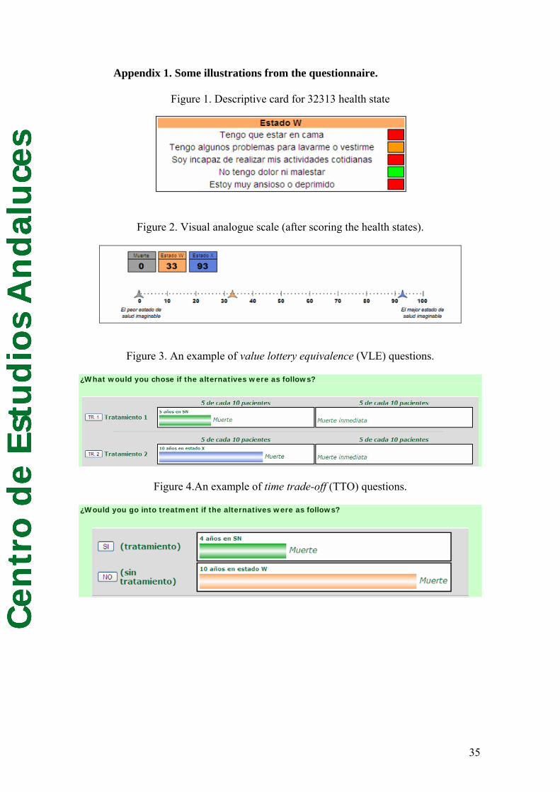
Appendix 1 provides some illustrations of the questions.

Section 1 described the 18 EQ-5D health states (Table 2) for which preferences

were elicited. This set of health states provides enough variability to encompass a wide

range of conditions. Each of the nine subsamples valued two health states, anonymously

labelled as X and W, respectively. They were assigned in such a way that health state X

was always logically better than state W. Respondents were asked to score both health

18

Cen

tro

de

Est

ud

ios

An

dal

uce

sstates by a visual analogue scale (VAS). This task was only included in order to help

people to familiarize with the health states.

[Insert Table 2 about here]

Section 3 administered the six unchained CE questions required to account for

utility curvature of the utility function for life years and also for testing QALY models.

The prospects for which we determined the certainty equivalents are displayed in Table

3. Section 5 collected some sociodemographic characteristics (gender, age, educational

level, income level, etc.) from subjects.

[Insert Table 3 about here]

The three methods applied (TTO, VLE, and CE) elicited preferences through a

sequence of choices. The use of choice-based mechanisms in order to find the

respondent’s indifference value is supported by two basic reasons. First, individual’s

choices are the primitive of utility theory, being the basis of decision theory. Second,

prior research by Bostic et al. (1990) showed that a choice-based procedure was more

consistent with simple choices than matching-based procedures. Both reasons support

the determination of indifferences through choices, as it is indeed done in many health

state utility measurements (Lener et al., 1998). Besides, choice-based procedures are

commonly implemented in a ‘transparent’ way, that is, respondents are aware that the

aim of the whole sequence of choices is to produce indifference. However, as Fischer et

al. (1999) showed, the more transparent the choice-based procedure is the larger the

discrepancy with respect to simple choices is. The discrepancy vanished when the aim

of the choice-based procedure remained ‘hidden’ to subjects, as indeed occurred with

the choice-based procedure used by Bostic et al. (1990). Braga and Starmer (2005)

argued in similar terms in favour of using opaque choice-based procedures in order to

avoid preference reversals in cost-benefit analysis.

19

Cen

tro

de

Est

ud

ios

An

dal

uce

sPrevious discussion motivated that we used a non-transparent choice-based

procedure. Specifically, we used the parameter estimation by sequential testing (PEST)

procedure to elicit preferences (Luce, 2000). This routine inserts filler questions

generated at random, forcing the respondent to evaluate each choice “as if” it was

independent from the rest of the sequence, and only converges to an indifferent point

when the responses become consistent (for details, see Appendix 2). To the best of our

knowledge, the only study related to the topic of this paper in which the PEST has been

applied, was the experiment conducted by Bleichrodt et al. (2005).

4.3 Analysis

We classified the respondents according to different criteria. First of all, for a given

health state, we identified those subjects who regarded it as better than death. In the

same way, we also identified those subjects who assessed the same health state as worse

than death. Henceforth, we will use the expressions better-than-death subjects and

worse-than-death subjects for referring to these two groups of respondents.

Afterwards, we classified both better and worse than death subjects according to

their attitudes towards risk. For better-than-death subjects, in order to account for

response error, we classified a subject as risk averse (risk seeking) if the certainty

equivalent in at least 4 out of 6 CE questions was lower (higher) than the expected value

of the risky prospect. For worse-than-death subjects, the classification of a subject as

risk averse (risk seeking) was the same except that now the certainty equivalent had to

be higher (lower) than the expected value of the prospect. Risk neutrality required in

both cases that the certainty equivalent was equal to the expected value of the prospect.

Finally, estimates for the curvature coefficient of the utility function of life

duration obtained through nonlinear least squares served to classify the respondents

20

Cen

tro

de

Est

ud

ios

An

dal

uce

saccording to the shape (concave, convex, linear) of such a utility function. This was

only done under rank-dependent utility, since under expected utility there is a one-to-

one relationship between risk attitude and shape of the utility function. For the power

function, this classification implies that a subject was classified as concave (convex,

linear) for better-than-death health states if the corresponding power estimate was less

than 0.95 (was greater than 1.05, was between 0.95 and 1.05). Worse-than-death

subjects were classified in the opposite way: concave (convex) utility required that the

power coefficient was larger than 1.05 (was less than 0.95). Health state utilities were

computed for each subject according to the formulas shown in Table 1.

QALY assumptions were tested by using two different non-parametric tests,

namely, the Wilcoxon signed-rank test and the Friedman test. A significance level of

10% was used in all cases..

The nonparametric Wilcoxon signed-rank test served to test for significance of

differences between responses given to the TTO and the VLE for a given health state,

within each subsample. This was the way in which the assumption of transferability

(Test 1) was tested. As noted in Section 3, the test was restricted to better-than-death

states.

The nonparametric Friedman test was used to test for significance of differences

among the proportional matches based on the twelve certainty equivalents that each

respondent provided. In such a way we checked whether the QALY model is linear

(Test 2). Notice that in this test we did not separate health state X from health state W

because linear utility function for life duration implies that preferences for life duration

are independent from severity of the health state. The test was performed, on the one

hand, with those respondents who regarded both state X and state W as better than death

21

Cen

tro

de

Est

ud

ios

An

dal

uce

sand, on the other, with those respondents who considered states X and W as worse than

death.

The assumption of multiplicativity (Test 3) was examined at the individual level.

The nonparametric Wilcoxon signed-rank test was used to test for significance of

differences between the six certainty equivalents elicited for health state X and the six

ones elicited for state W for each respondent. Next we computed the percentage of

subjects for which we could not reject the null hypothesis of equality between CEs. All

these comparisons were performed separating respondents who regarded both health

states as better than death from those who regarded the states as worse than death.

Note that the outcomes included in Table 3 allow for testing the functional form

of the utility of life duration (Tests 4 and 5). For example, since outcomes of prospect 3

follow from adding two years to outcomes of prospect 2, and outcomes in the latter

follow from adding the same amount to outcomes belonging to prospect 1, two tests of

constant risk posture (Test 4) result. Prospects 1 and 3, 4 and 5, and also 5 and 6, can be

also compared in a similar way. In short, we have five tests of constant risk posture per

health state as a result of comparing the following proportional matches: PM1 vs PM2,

PM2 vs PM3, PM1 vs PM3, PM4 vs PM5, and PM5 vs PM6, where the subscript

denotes the prospect concerned according to numeration used in Table 3. Constant

proportional risk posture (Test 5) was tested by comparing the following proportional

matches for each health state: PM1 vs PM4, PM3 vs PM6, and PM2 vs PM5. Again, we

performed the tests keeping apart people who regarded a health state as better than death

from those who regarded the same state as worse than death.

5. Results

5.1 Sample

22

Cen

tro

de

Est

ud

ios

An

dal

uce

sObservations from 656 subjects were finally used in the data analysis. Sixty four

individuals were excluded because of various types of inconsistencies. Firstly, thirty-

four participants assigned higher valuations to the health state W than to the state X

(remember that all pairs of health states can be logically rank ordered). Six out of those

thirty-four were inconsistent in their VAS valuations, thirteen in the TTO responses and

the fifteen remaining in the VLE task. On the other hand, thirty individuals who had

regarded one of the health states as worse than death with one of the methods applied

(TTO, VLE, and CE), considered the same state as better than death with another

method. This type of ‘preference reversal’ occurred between TTO and VLE for thirteen

individuals, and between CE and one of the two mentioned for the other seventeen

subjects. The main characteristics of the final sample are shown in Table 4. The

representativeness of the sample was hardly affected as a result of the exclusions.

[Insert Table 4 about here]

5.2 Risk attitude towards life years in better and worse than death health states

Table 5 classifies the respondents in terms of their risk attitude. As it was expected,

there were quite a lot more respondents regarding health state W (the more serious

condition) as worse than death (315) than those who considered health state X as less

preferred to death (8). Only four of the X states (i.e., 11113, 11131, 13212, and 11312)

contained some worse-than-death subject, with a maximum of 3 worse-than-death

subjects for state 13212. On the contrary, all the W states included some worse-than-

death respondent (the minimum was 3 subjects for health state 13311).

[Insert Table 5 about here]

Table 5 shows a twofold pattern of risk attitudes. Better-than-death respondents

mostly exhibited risk aversion (concave utility under expected utility), whereas worse-

than-death subjects behaved as risk seekers (convex utility under expected utility). The

23

Cen

tro

de

Est

ud

ios

An

dal

uce

sonly exception to this rule occurs with the health state 32223, for which the reverse

pattern is found. It is interesting to notice that this twofold pattern resembles previous

evidence in the domain of money, where various studies (Fishburn and Kochenberger,

1979, Pennings and Smidts, 2003) have found concave utility for positive outcomes (or

gains) and convex utility for negative outcomes (or losses), under expected utility. This

similarity could suggest that the zero duration (or the death) may act as a threshold, thus

making that the same life duration is perceived as a positive duration (a gain) or a

negative duration (a loss) according to the severity of the health state. It has to be

emphasized that this phenomenon of ‘sign-dependence’ should be viewed as an

indication of a multiplicative relationship between duration and health status

(Miyamoto, 1999) rather than as an expression of some type of ‘maximum endurable

time’ (Sutherland et al., 1982). Maximum endurable time is an example of non-

monotonic preferences for life duration, which is different from the coexistence of

better and worse than death health states.

5.3 Axiomatic tests

The assumption of transferability (Test 1) holds for eleven of the eighteen states.

That is, for these health states, the hypothesis of equality in the responses given to the

TTO and the VLE methods cannot be rejected. Nevertheless, there are seven states

(more than one third) for which TTO and VLE valuations significantly differ (Wilcoxon

signed-rank test, p < 0.0001). Most of these health states (6 out of 7) could be labeled as

‘moderate’ or ‘severe’, according to the classification that Dolan (1997) coined when

modeling the EQ-5D system. Thus, although transferability seems to be an acceptable

assumption for the majority of health states used in this study, this does not hold for a

significant percentage (around 39%) of the selection. This evidence suggests that the

24

Cen

tro

de

Est

ud

ios

An

dal

uce

scommon practice of using TTO utilities to make decisions under risk is not probably

right in all the cases.

As noted in Section 3.1, under rank-dependent utility assumptions it is necessary

to distinguish between better-than-death and worse-than-death health states because

probability weights are dependent on the rank order of the outcomes. Therefore we have

to set apart both domains, Ω+ and Ω-, in order to test QALY assumptions. As there were

only eight respondents who regarded both health state X and health state W as worse

than death2, we opted for omitted them from the tests of linearity (Test 2) and

multiplicativity (Test 3) assumptions. Since the tests of constant (Tests 4) and

proportional risk posture (Test 5) were performed at health state level we had not to

restrict our attention to subjects who regarded X and W together as better or as worse

than death health states. We only removed from these tests the same eight respondents

as before.

The non parametric Friedman test rejects the assumption of linearity for the

utility function of life in five out of nine subsamples displayed in Table 2 (groups 1, 2,

3, 4, and 7). This encompasses almost 75% of better-than-death subjects (249/341).

Hence we find a broad rejection to the assumption of linear utility for life years under

both expected utility and rank-dependent utility. Conversely, multiplicativity (Test 3) is

strongly supported at individual level. Wilcoxon signed-rank tests suggest that the null

hypothesis (equal distributions of CEs for X and for W) cannot be rejected for the

91.40% of the better-than-death respondents (319/341). This finding is consistent with

the idea noted in Section 5.2 about that better and worse than death health states are

examples of diagnostic of a multiplicative QALY model.

2 These subjects are the eight respondents that valued states type X 11113, 11131, 13212, and 11312 as worse than death. The same subjects regarded the corresponding states type W 32223, 23232, 33333, and 33323 in the same way.

25

Cen

tro

de

Est

ud

ios

An

dal

uce

sFinally, we found that proportional risk posture clearly outperformed constant

risk posture. Overall, the proportional risk posture assumption is not rejected in 68 out

of 81 possible comparisons (83.95%) of the PMs, with percentages for better-than-death

and worse-than-death subjects of 85.19% and 81.48%, respectively. On the contrary, we

only found support to the hypothesis of constant risk attitude in 62 out of 135 possible

comparisons (45.93%). In this case, percentages were 44.44% for better-than-death

subjects and 48.89% for worse-than-death subjects. Therefore, we found strong

nonparametric evidence consistent with a power specification for the utility function of

life years. Thus, we will assume in the following this functional form in order to

account for utility curvature of life duration in the calculations of health state utilities.

5.4 Health state utilities under expected utility and linear QALY model

Table 6 shows median utilities for the 18 health states obtained under the same

three paradigms which were previously considered in Table 1, i.e., expected utility and

linear QALY model (EU-linear), expected utility and power QALY model (EU-power),

and rank-dependent utility and power QALY model (RDU-power).

[Insert Table 6 about here]

The inspection of the results for ‘EU-linear’ reveals that the highest median

value corresponds to the EQ-5D health state 11112 (HTTO=0.9167 and HVLE=0.9083).

The worst valued state is the ‘pits state’ (33333), with median utilities of –0.3333 for

VLE and –0.8125 for TTO method. It is noticeable that there are no logical

inconsistencies between median values. That is, considering the 73 pairs of health states

which can be logically compared one to each other (e.g., 11112 vs 11113), the logically

better state has been valued higher than the logically worse one, for both TTO and VLE

methods. Differences arise, however, when both type of utilities are compared within

26

Cen

tro

de

Est

ud

ios

An

dal

uce

seach health state. We found significant differences for the half of the health states. Most

the differences concern states type W (all of them except for state 22222 and state

32223). States type X 12111 and 13212 have to be added to the seven remaining states

type W. Notice, however, that this comparison is done for the whole sample, without

distinguishing between better and worse than death subjects. When such distinction is

made, we obtain for better-than-death subjects the same results that we found when the

assumption of transferability was tested.

5.5 Health state utilities under expected utility and power QALY model

We assumed a power specification to calculate health state utilities by relaxing

the assumption of linear utility function for life duration. Two power coefficients were

estimated for each subject, one for each of the health states (X and W) they assessed. In

the case of EU-power, the overall median estimate for the power coefficient was 0.638.

At health state level, all the median estimates were below 1, except for health state

32223 whose estimate was significantly above the unity. Median estimate for better-

than-death subjects was of 0.61, whereas the one for worse-than-death subjects was of

0.747. These estimates predict concavity and convexity respectively, since they are

using in different domains (positive the first, negative the second) of the utility plane.

Therefore, in agreement with previous evidence assuming expected utility (e.g.,

Stiggelbout et al., 1994) we find strong support for concave utility of life duration in the

domain of better-than-death health states. The finding of a mean estimate predicting

convexity for worse-than-death subjects is consistent with the results described

previously in Table 5. The calculation of health state utilities assuming individual

estimates for the power utility function of life years yielded a new set of values for TTO

and VLE, as it can be seen in column ‘EU- power’ in Table 6.

27

Cen

tro

de

Est

ud

ios

An

dal

uce

sMost of the new TTO utilities significantly differ from those calculated under

‘EU-linear’. Only for health states 32223, 32313, and 33323 differences remained non-

significant. A similar finding arises for VLE utilities, sharing the three previous states

plus health state 23232. It is apparent then that, under expected utility, the largest

discrepancies between linear and power utilities emerged for mild and moderate health

states above all. When TTO and VLE utilities are compared, once they have been

adjusted by utility curvature, we found a very similar result that that was obtained under

‘EU-linear’. Discrepancies hold for the same health states as for ‘EU-linear’ except for

states 11133 and 33323 for which now there is no significant difference.

5.6 Shape of the utility function of life duration and probability weights

Table 7 shows the classification of the subjects based on the individual power

coefficients estimated under rank-dependent utility. The dominant pattern was concave

utility for better-than-death subjects and convex utility for worse-than-death subjects.

Hence, the general pattern remains the same as it was under expected utility.

[Insert Table 7 about here]

However, if Table 7 is compared with Table 5 we then obtain some indication

that the equivalence between risk aversion and concave utility under rank-dependent is

not so straightforward as under expected utility was. For health states type X, the

proportion of better-than-death respondents with convex and mixed utility was

significantly higher than that for risk lovers and risk neutrals subjects in Table 5 (31.4%

vs 12.81%). There was also a minor variation in health state W, but it was not

significant. For worse-than-death respondents, the number of subjects with convex and

linear utility was also larger than under expected utility (in the case of the health state

28

Cen

tro

de

Est

ud

ios

An

dal

uce

sW). As only eight respondents regarded state X as worse than death, the comparison

between the two tables does not reveal any relevant change.

The different proportions found under each utility theory, may in principle be

attributed to the fact that under rank-dependent utility the probability weight reflects

part of the risk attitude that under expected utility is completely encapsulated in the

utility function. The impact of probability weighting, however, is not enough powerful

as to reverse the modal pattern from expected utility to rank-dependent utility, except

for one of the health states. In the case of state 32223, a reversion of preferences occurs,

in the sense that although better-than-death (worse-than-death) subjects are risk seekers

(risk averse) they have concave (convex) utility under rank-dependent utility. To the

best of our knowledge, this is the first time that the coexistence of risk seeking (risk

aversion) and concave (convex) utility has been found for health outcomes. Abdellaoui

et al. (2008) recently reported similar evidence with money outcomes.

Overall median estimate for the power coefficient under rank-dependent utility

(βRDU) is 0.784, with median w(0.5) equals to 0.444. Therefore, although our data do not

provide information on the whole probability weighting function, but only for the

specific probability value of p=0.5, our overall estimate for w(0.5) is consistent with an

inverse S-shaped probability weighting function, in a similar way that Abdellaoui et al.

(2008) found for money outcomes. Median estimates of βRDU for better-than-death and

for worse-than-death subjects were respectively 0.786 and 0.782. Both median estimates

exceed those obtained under expected utility, above all the former.

Since the probability weights are dependent on the rank order of outcomes, it is

interesting to realise how median estimates for w(0.5) behave when better and worse

than death subjects are separated. Remember (Section 3.1) that underweighting of

p=0.5 leads to a different prediction on the relationship between βEU and βRDU

29

Cen

tro

de

Est

ud

ios

An

dal

uce

saccording to the assessment of the health state as better or worse than death. When

attention is restricted to better-than-death subjects, we found that the median estimate

for w(0.5) was 0.43. Hence, in broad terms, it seems that because of the underweighting

of p=0.5, the analysis of data under expected utility leads to overestimate the concavity

of the utility function for life duration (βEU=0.61 < βRDU = 0.786). This lower concavity

under non-expected utility is broadly consistent with the findings reported by Bleichrodt

and Pinto (2005).

The picture was rather different for worse-than-death subjects. In this case, there

was hardly evidence of probability transformation of p=0.5 in terms of the median

estimate. Notwithstanding, this aggregate finding hides substantial variability at

individual level, as it is usual in empirical exercises in which group estimates are

calculated as a median or average of the subjects’ estimates. In this study, variability

means that we found some less of one-third of worse-than-death respondents whose

probability weight was above 0.5, whereas the contrary, i.e., w(0.5)<0.5, can be held

roughly for the half of the sample. The net effect of these opposite forces is that the

median transformation of p=0.5 is approximately linear. For this reason, the median

power coefficient estimated under rank-dependent for worse-than-death subjects is

much closer to that obtained under expected utility (βEU=0.747 and βRDU = 0.782).

The previous finding apparently contradicts the assumption of an inverse S-

shaped probability weighting function with a point lying between 0.3 and 0.4 for which

the function changes from overweighting probabilities to underweighting probabilities.

To test the robustness of this result, and taking into account that there were less worse-

than-death subjects than better-than-death subjects, we recalculated the median estimate

for w(0.5) only for those health states in which there had forty or more worse-than-death

respondents (i.e., states 23232, 32223, 32313, 33323, and 33333). The resulting

30

Cen

tro

de

Est

ud

ios

An

dal

uce

sestimate (0.47) suggested small but significant underweighting (p=0.03), being coherent

with the typical form of the probability weighting function. This finding suggests that in

those health states in which there were less worse-than-death subjects, there was

overweighting of probability.

5.7 Health state utilities under rank-dependent utility and power QALY model

The health state utilities estimated under ‘RDU-power’ are also shown in Table

6. Median values are for the most part significantly different from those obtained under

expected utility, but the ranking of the health states remains widely unchanged. The

pattern previously described for expected utility is now intensified under rank-

dependent utility: the difference between linear and power utilities is significant for all

the health states except for the state 32313 (for TTO utilities) and the state 23232 (for

VLE utilities). The picture hardly changes when TTO utilities calculated under ‘EU-

power’ and ‘RDU-power’ paradigms are compared each other. There are only two states

for which no significant difference is found (32313 and 33323) for the TTO method.

The same can be stated for VLE utilities: we cannot reject the hypothesis of null

differences for three health states (23232, 32223, and 32313). When both elicitation

methods are directly compared, we find that the number of health states for which there

are significant differences falls from nine to seven, with respect to ‘EU-power’ and

‘EU-linear’. Such health states are the following: 12111, 13212, 13311, 23232, 32211,

33323, and 33333.

6. Discussion

We set five main objectives in the introduction of this manuscript. First of them was the

aim of applying a new method to account for curvature of the utility function of life

31

Cen

tro

de

Est

ud

ios

An

dal

uce

sduration in order to adjust health state utilities. Bleichrodt and Pinto (2006) stated that

the utility function for life years “can generally be approximated to a reasonable degree

by performing five to six preference measurements”. The method employed in the study

reported in this paper, and first proposed by Miyamoto (2000), used six certainty

equivalence questions to get that “reasonable approximation”. Such a procedure has the

advantages of not being susceptible to error propagation, and to avoid biases due to

probability weighting, one of the main deviations from expected utility.

Group estimates obtained with the new adjustment method were, in general,

consistent with previous evidence, since that better-than-death subjects (those with an

increasing utility function of duration) exhibited concave utility for both expected utility

and rank-dependent utility, the two theories considered in this paper. As it was

expected, the estimate for the power coefficient was significantly higher for rank-

dependent utility than for expected utility. This finding confirms previous parametric

estimations performed by Bleichrodt and Pinto (2005) under rank-dependent utility. In

fact, the median estimate obtained in the present study was very similar to those

estimated by them. Apart from that, although the procedure applied is not intended to

estimate the probability weighting function, the median estimate for probability p=0.5 is

broadly consistent with an inverse S-shaped probability weighting function.

The second aim of this paper was to provide evidence on the validity of a

common practice in economic evaluation of health programmes, consisting in freely

transferring utilities derived from a riskless context to a decision context under risk.

This is indeed an assumption underlying a so extensively used multiattribute system as

the EQ-5D is. The assumption of transferability has been tested before (Bleichrodt and

Johannesson, 1997; Abellan et al., 2007) by using the time trade-off and the standard

gamble methods. Both studies provided some evidence against the validity of

32

Cen

tro

de

Est

ud

ios

An

dal

uce

stransferability. Other studies, employing different elicitation methods (e.g., Stalmeier

and Bezembinder, 1999) have found evidence supporting the idea of a ‘unified’ concept

of utility. The test reported in this paper is, in some respect, more demanding than the

previous ones. We used an elicitation method framed in terms of risk (called value

lottery equivalence) which is a monotonic transformation of the time trade-off. As the

framing of the time trade-off and the framing of the value lottery equivalence are

similar, discrepancies between the indifference responses elicited by the two methods

are more troublesome than those which could be obtained between the time trade-off

and the standard gamble. Our data show that transferability was violated for seven out

of eighteen possible health states. This finding suggests that, although transferability

may work in many cases, it may be also violated by a significant number of people.

Thus, our results claim cautious in transferring utilities across riskless and risky

contexts.

The three last issues focused on in this paper concerning the validity of three

assumptions of the QALY model. Our findings are straightforward for the three tests we

performed. Linearity of the utility function for life duration is firmly rejected by testing

a very simple axiomatic condition, not previously tested yet. Hence, this finding adds to

the previous one due to Bleichrodt and Pinto (2005) by using a different test and a quite

a lot larger sample than they used. Therefore, hope for the linear QALY model only

remains in the realm of prospect theory (Doctor et al., 2004). On the contrary, the

property of multiplicativity (that is, that utility curvature is independent on the severity

of the health status) is widely supported by our data. It has to be noted, however, that

we only performed within-subject tests of multiplicativity. Hence, we cannot discard

that differences may exist among curvature parameters estimated from different

samples. Finally, we found strong support to a power specification for the utility

33

Cen

tro

de

Est

ud

ios

An

dal

uce

sfunction of life duration. Previous evidence (Miyamoto and Eraker, 1989) by testing the

same assumption as ours (proportional risk posture) was negative, which may be related

to the scarce sample size used.

The fact that this study has been based on a large survey of general population

permits to provide of more robustness some previous findings. This is the case of our

results in favour of multiplicativity and against linearity. At the same time, we think that

our database provides insight in topics where previous investigations have failed. This is

the case of our substantial support to a power utility function in opposition to an

exponential utility function.

Obviously, as always happens, this study has some limitations. Probably the

most important drawback is that we have only considered rank-dependent utility as an

alternative to expected utility. This implies that the estimation of the curvature

parameter of the utility function for life years has only accounted for probability

weighting, but not for loss aversion. Previous empirical evidence (Bleichrodt et al.,

2007) seems to suggest that loss aversion is a driver of biases for some risky methods,

such as the certainty equivalence and the standard gamble. It is less clear, however, if a

method involving two prospects such as the value lottery equivalence may be affected

by loss aversion. Any way, we think that is preferable to correct some biases, even

though other possible remain active, rather than to trust in that, for example, upwards

and downwards biases offset.

34

Cen

tro

de

Est

ud

ios

An

dal

uce

sAppendix 1. Some illustrations from the questionnaire.

Figure 1. Descriptive card for 32313 health state

Figure 2. Visual analogue scale (after scoring the health states).

Figure 3. An example of value lottery equivalence (VLE) questions.

¿What would you chose if the alternatives were as follows?

Figure 4.An example of time trade-off (TTO) questions.

¿Would you go into treatment if the alternatives were as follows?

35

Cen

tro

de

Est

ud

ios

An

dal

uce

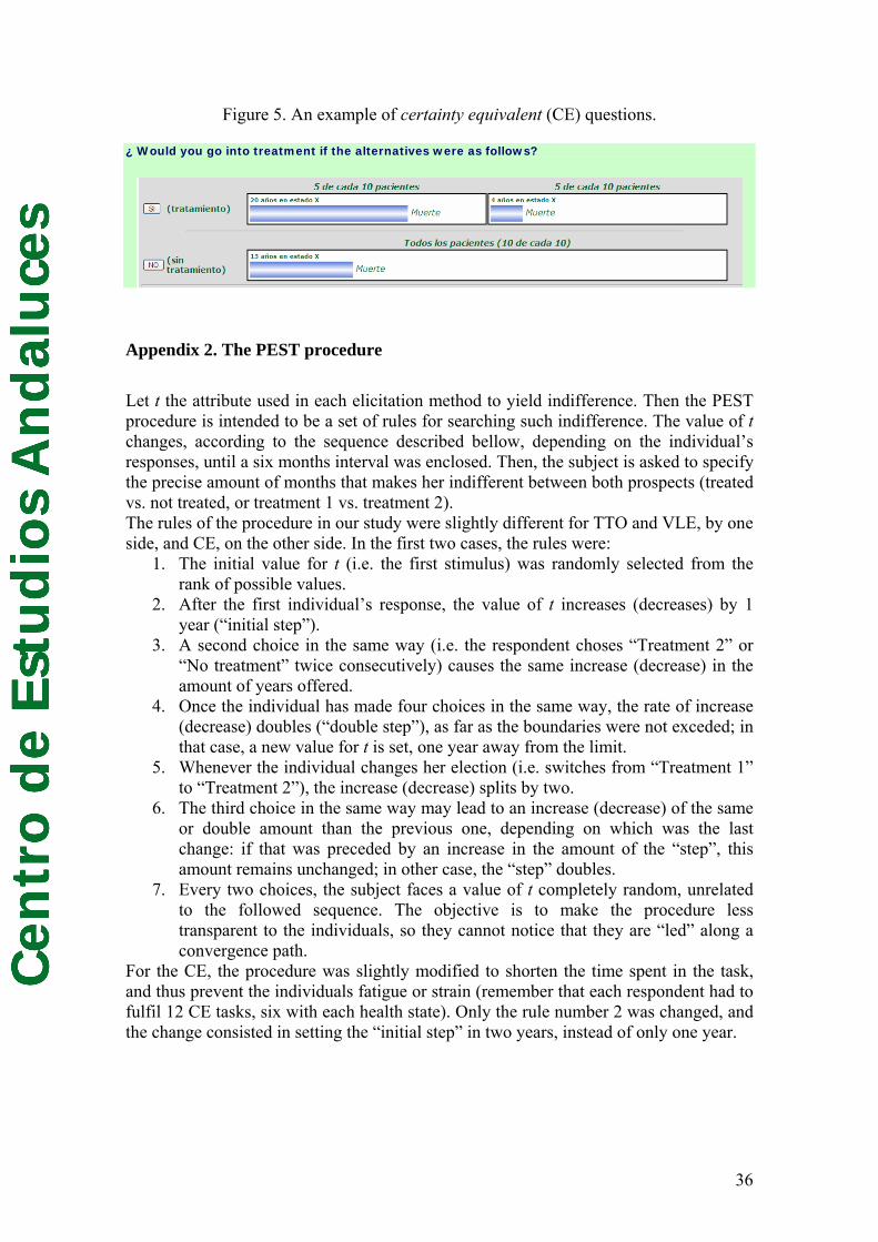
sFigure 5. An example of certainty equivalent (CE) questions.

¿ Would you go into treatment if the alternatives were as follows?

Appendix 2. The PEST procedure

Let t the attribute used in each elicitation method to yield indifference. Then the PEST procedure is intended to be a set of rules for searching such indifference. The value of t changes, according to the sequence described bellow, depending on the individual’s responses, until a six months interval was enclosed. Then, the subject is asked to specify the precise amount of months that makes her indifferent between both prospects (treated vs. not treated, or treatment 1 vs. treatment 2). The rules of the procedure in our study were slightly different for TTO and VLE, by one side, and CE, on the other side. In the first two cases, the rules were:

1. The initial value for t (i.e. the first stimulus) was randomly selected from the rank of possible values.

2. After the first individual’s response, the value of t increases (decreases) by 1 year (“initial step”).

3. A second choice in the same way (i.e. the respondent choses “Treatment 2” or “No treatment” twice consecutively) causes the same increase (decrease) in the amount of years offered.

4. Once the individual has made four choices in the same way, the rate of increase (decrease) doubles (“double step”), as far as the boundaries were not exceded; in that case, a new value for t is set, one year away from the limit.

5. Whenever the individual changes her election (i.e. switches from “Treatment 1” to “Treatment 2”), the increase (decrease) splits by two.

6. The third choice in the same way may lead to an increase (decrease) of the same or double amount than the previous one, depending on which was the last change: if that was preceded by an increase in the amount of the “step”, this amount remains unchanged; in other case, the “step” doubles.

7. Every two choices, the subject faces a value of t completely random, unrelated to the followed sequence. The objective is to make the procedure less transparent to the individuals, so they cannot notice that they are “led” along a convergence path.

For the CE, the procedure was slightly modified to shorten the time spent in the task, and thus prevent the individuals fatigue or strain (remember that each respondent had to fulfil 12 CE tasks, six with each health state). Only the rule number 2 was changed, and the change consisted in setting the “initial step” in two years, instead of only one year.

36

Cen

tro

de

Est

ud

ios

An

dal

uce

s

References

Abdellaoui M (2000). Parameter-free elicitation of utilities and probability weighting

functions. Management Science 46, 1497–1512.

Abdellaoui M, Bleichrodt H, L’Haridon O (2008). A tractable method to measure utility

and loss aversion under prospect theory. Journal of Risk and Uncertainty 36, 245-266.

Abdellaoui, M., Barrios C., Wakker P. P. (2007). Reconciling introspective utility with

revealed preference: Experimental arguments based on prospect theory. Journal of

Econometrics 138, 356-378.

Abellan-Perpinan, J.M., Bleichrodt, H., Pinto, J.L. (2007). Testing the predictive

validity of the time trade-off and the standard gamble. Working paper, CENTRA,

E2007/14.

Attema AE, Brouwer WBF (2009). The correction of TTO-scores for utility curvature

using a risk-free utility elicitation method. Journal of Health Economics 28, 234-243.

Attema, A.E., Bleichrodt, H.,Wakker, P.P. (2007).Measuring the utility of life duration

in a risk-free versus a risky situation.Working paper, Erasmus University Rotterdam.

Bleichrodt H, Abellan-Perpiñan JM, Pinto JL, Mendez I. (2007) Resolving

Inconsistencies in Utility Measurement under Risk: Tests of Generalizations of

Expected Utility. Management Science; 53: 469-482.

Bleichrodt H, Doctor J, Stolk E (2005). A nonoparametric elicitation on the equity-

efficiency trade-off in cost-utility analysis. Journal of Health Economics 24, 655-678.

Bleichrodt H, Johannesson M. The Validity of QALYs: An Empirical Test of Constant

Proportional Tradeoff and Utility Independence. Medical Decision Making 1997; 17:

21-32.

Bleichrodt H, Pinto JL (2006). Conceptual Foundations for Health Utility Measurement.

37

Cen

tro

de

Est

ud

ios

An

dal

uce

sIn Jones A (ed.). The Elgar Companion to Health Economics. Edward Elgar Publishing

Limited.

Bleichrodt H, Pinto JL. (2000) A Parameter-Free Elicitation of the Probability

Weighting Function in Medical Decision Analysis. Management Science,46:1485-1496.

Bleichrodt H, Pinto JL. The Validity of QALYs under Nonexpected Utility. The

Economic Journal 2005,115: 533-550.

Bleichrodt H. (2002) A new explanation for the difference between time trade-off

utilities and standard gamble utilities. Health Economics; 11: 447-456.

Bleichrodt, H. (2001). Probability weighting in choice under risk: an empirical test.

Journal of Risk and Uncertainty, 23, 185-198.

Bleichrodt, H. and Johannesson, M. (1997). The Validity of QALYs: An Empirical Test

of Constant Proportional Tradeoff and Utility Independence. Medical Decision Making,

17, 21-32.

Bleichrodt, H. and Schmidt, U. (2002). A context-dependent model of the gambling

effect. Management Science, 48, 802-812.

Bostic, R., Hernstein, R. J. and Luce, R. D. (1990). The effect on the preference reversal

phenomenon of using choice indifferences. Journal of Economic Behavior and

Organization 13, 193-212.

Braga J, Starmer C (2005). Preference anomalies, preference elicitation and the

discovered preference hypothesis. Environmental and Resource Economics 32, 55-89.

Doctor JN, Bleichrodt H, Miyamoto J, Temkin N, Dikmen S. (2004) A New and More

Robust Test of QALYs. Journal of Health Economics; 353-367.

Dolan P. (1997) Modelling valuations for EuroQol health states. Medical Care; 35:

1095-1108.

Fischer, G. W., Carmon, Z., Ariely, D., and Zauberman, G. (1999). Goal-based

38

Cen

tro

de

Est

ud

ios

An

dal

uce

sConstruction of Preferences: Task Goals and the Prominence Effect. Management

Science, 45, 1057-1075.

Gonzalez R, Wu G (1999). On the shape of the probability weighting function.

Cognitive Psychology 38, 129-166.

Keeney, R. and Raiffa, H. (1976). Decisions with multiple objectives. New York,

Wiley.

Lener LA, Cher DJ, Goldstein MK, Bergen MR, Garber A (1998). The effect of search

procedures on utility elicitations. Medical Decision Making 18, 76-83.

Llewellyn-Thomas, H. A., Sutherland, H. J., Tibshirani, R., Ciampi, A., Till, J. E. and

Boyd, N.F. (1982). The Measurement of Patients' Values in Medicine. Medical

Decision Making, 2, 449-462.

Luce RD. (2000) Utility of Gains and Losses: Measurement-Theoretical and

Experimental Approaches. New Jersey: Lawrence Erlbaum Associates, Inc.,.

Martin, A.J., Glasziou, P.P., Simes, R.J., Lumley, T. (2000). A comparison of standard

gamble, time trade-off, and adjusted time trade-off scores. International Journal of

Technology Assessment in Health Care 16 (1), 137–147.

McNeil, B. J., Weichselbaum R., and Pauker S. G. (1978). Fallacy of five-year survival

in lung cancer. New England Journal of Medicine, 299, 1397-1401.

Miyamoto JM, Eraker SA. (1988) A multiplicative model of the utility of survival

duration and health quality. Journal of Experimental Psychology: General; 117: 3-20.

Miyamoto JM, Eraker SA. (1985) Parameter Estimates for a QALY Utility Model.

Medical Decision Making, 5: 191-213.

Miyamoto JM. (1999) Quality-adjusted life years (QALY) utility models under

expected utility and rank-dependent utility assumptions. Journal of Mathematical

Psychology; 43: 201-237.

39

Cen

tro

de

Est

ud

ios

An

dal

uce

sMiyamoto JM. (2000) Utility assessment under expected utility and rank-dependent

utility assumptions. En: Chapman GB, Sonnenberg FA (eds). Decision Making in

Health Care, Cambridge University Press: Cambridge.

Miyamoto, J. M. (2000). Utility assessment under expected utility and rank dependent

utility assumptions. In G. B. Chapman and F. Sonnenberg. Decision making in health

care: Theory, psychology, and applications. New York: Cambridge University Press,

65-109.

Miyamoto, J. M. and Eraker, S. A (1985). Parameter Estimates for a QALY Utility

Model. Medical Decision Making, 5, 191-213.

Miyamoto, J. M. and Eraker, S. A. (1989). Parametric Models of the Utility of Survival

Duration: Tests of Axioms in a Generic Utility Framework. Organizational Behavior

and Human Decision Processes, 44, 166-202.

Oliver A (2005). Testing the internal consistency of the lottery equivalents method

using health outcomes. Health Economics 14, 149-159.

Oliver, A. (2003). The internal consistency of the standard gamble: tests after adjusting

for prospect theory. Journal of Health Economics, 22, 659-674.

Plott, C. P. (1996). Rational individual behavior in markets and social choice processes.

Arrow, K. J. Colombatto, E. Perlman, M. and Schmidt, C. eds. (1996) The Rational

Foundations of Economic Behavior: Proceedings of the IEA Conference Held in Turin,

Italy. St Martin’s Press, New York, 225–250.

Quiggin J. (1981) Risk perception and risk aversion among Australian farmers.

Australian Journal of Agriculture Economics; 25: 160–169.

Stalmeier, P. F. M., Bezembinder T. G. G., and Unic I. J. (1996). Proportional

Heuristics in Time Trade Off and Conjoint Measurements. Medical Decision Making,

16, 36-44.

40

Cen

tro

de

Est

ud

ios

An

dal

uce

sStalmeier, P.F. and Bezembinder, T. G. (1999). The discrepancy between risky and

riskless utilities: a matter of framing?. Medical Decision Making 19(4), 435-447.

Stiggelbout, A. M., Kiebert, G. M., Kievit, J., Leer, J. W. H., Stoter, G. and de Haes, J.

C. J. M. (1994). Utility Assessment in Cancer Patients: Adjustment of Time Tradeoff

Scores for the Utility of Life Years and Comparison with Standard Gamble Scores.

Medical Decision Making, 14, 82-90.

Sutherland, H. J., Llewellyn-Thomas, H., Boyd, N. F. and Till, J. E. (1982). Attitudes

towards quality of survival: The concept of “maximum endurable time”. Medical

Decision Making, 2, 299-309.

Torrance GW. (1986) Measurement of health-state utilities for economic appraisal: A

review. Journal of Health Economics; 5: 1-30.

Tversky A, Kahneman D. (1992) Advances in prospect theory: Cumulative

representation of uncertainty. Journal of Risk and Uncertainty, 5:297-323.

van Osch, S. M. C., Wakker P. P., van den Hout W. B., Stiggelbout A. M. (2004).

Correcting biases in standard gamble and time tradeoff utilities. Medical Decision

Making 24, 511-517.

Wakker P, Stiggelbout A. (1995) Explaining distorsions in utility elicitation through the

rank-dependent model for risky choices. Medical Decision Making; 15: 180-186.

Wakker, P. (1994). Separating marginal utility and probabilistic risk aversion. Theory

and Decision, 36, 1-44.

41

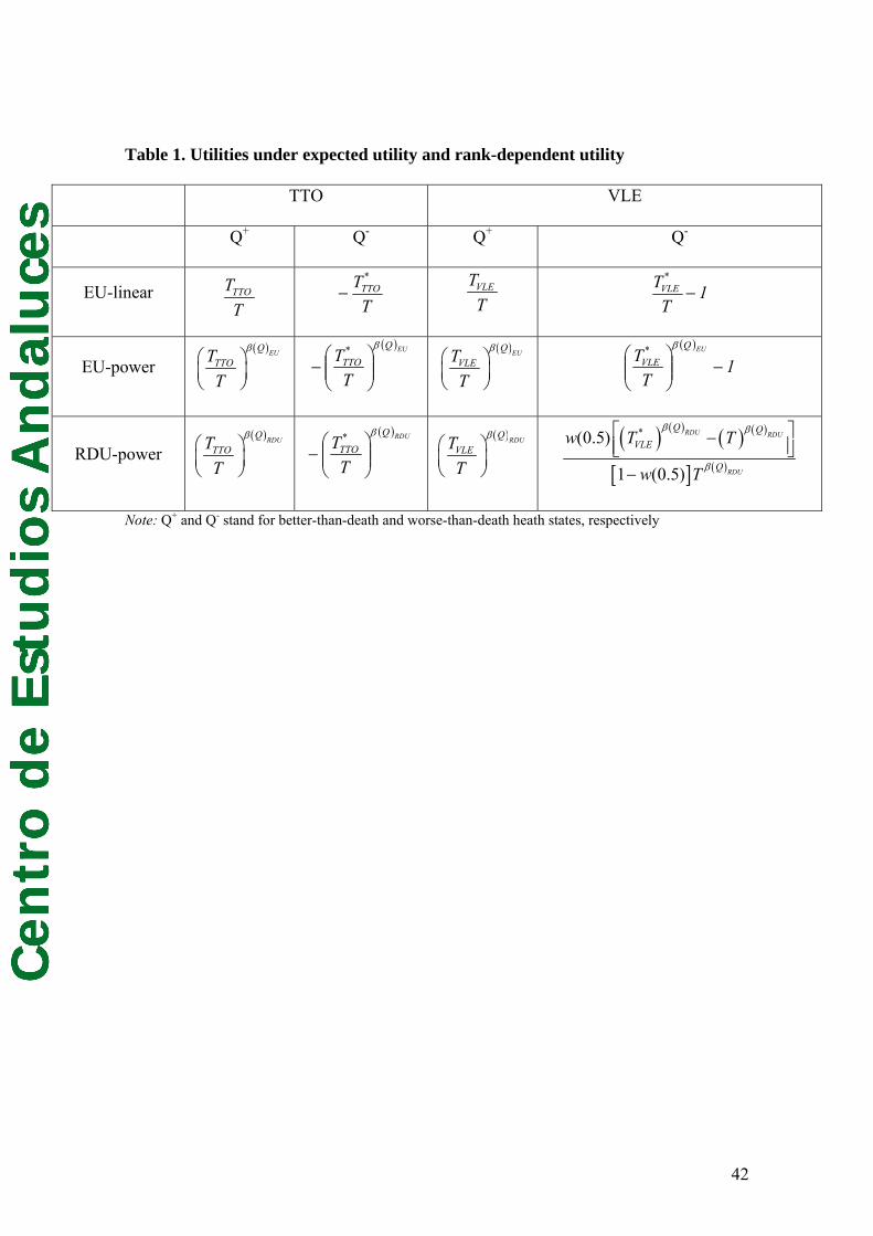
Cen

tro

de

Est

ud

ios

An

dal

uce

s

Table 1. Utilities under expected utility and rank-dependent utility

TTO VLE

Q+ Q- Q+ Q-

EU-linear TTOTT

TT*

TTO− VLETT

1T

T*VLE −

EU-power ( )EUQ

TTOTT

β⎛ ⎞⎜ ⎟⎝ ⎠

( )EUQ*

TTO

TT

β

⎟⎟⎠

⎞⎜⎜⎝

⎛−

( )EUQVLETT

β⎛ ⎞⎜ ⎟⎝ ⎠

( )

1T

T EUQ*VLE −⎟⎟

⎠

⎞⎜⎜⎝

⎛β

RDU-power ( )RDUQ

TTOTT

β⎛ ⎞⎜ ⎟⎝ ⎠

( )RDUQ*

TTO

TT

β

⎟⎟⎠

⎞⎜⎜⎝

⎛−

( )RDUQVLETT

β⎛ ⎞⎜ ⎟⎝ ⎠

( ) ( ) ( ) ( )

[ ] ( )

*(0.5)

1 (0.5)

RDU RDU

RDU

Q QVLE

Q

w T T

w T

β β

β

⎡ ⎤−⎢ ⎥⎣ ⎦−

Note: Q+ and Q- stand for better-than-death and worse-than-death heath states, respectively

42

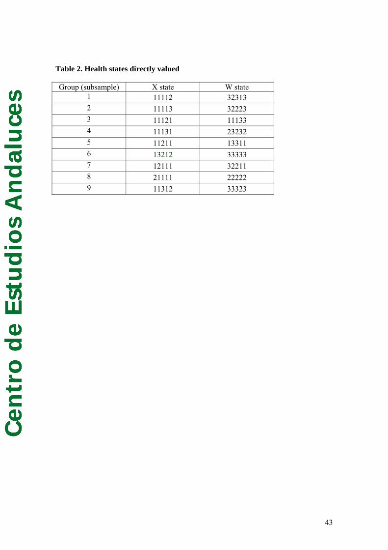
Cen

tro

de

Est

ud

ios

An

dal

uce

s

Table 2. Health states directly valued

Group (subsample) X state W state 1 11112 32313 2 11113 32223 3 11121 11133 4 11131 23232 5 11211 13311 6 13212 33333 7 12111 32211 8 21111 22222 9 11312 33323

43

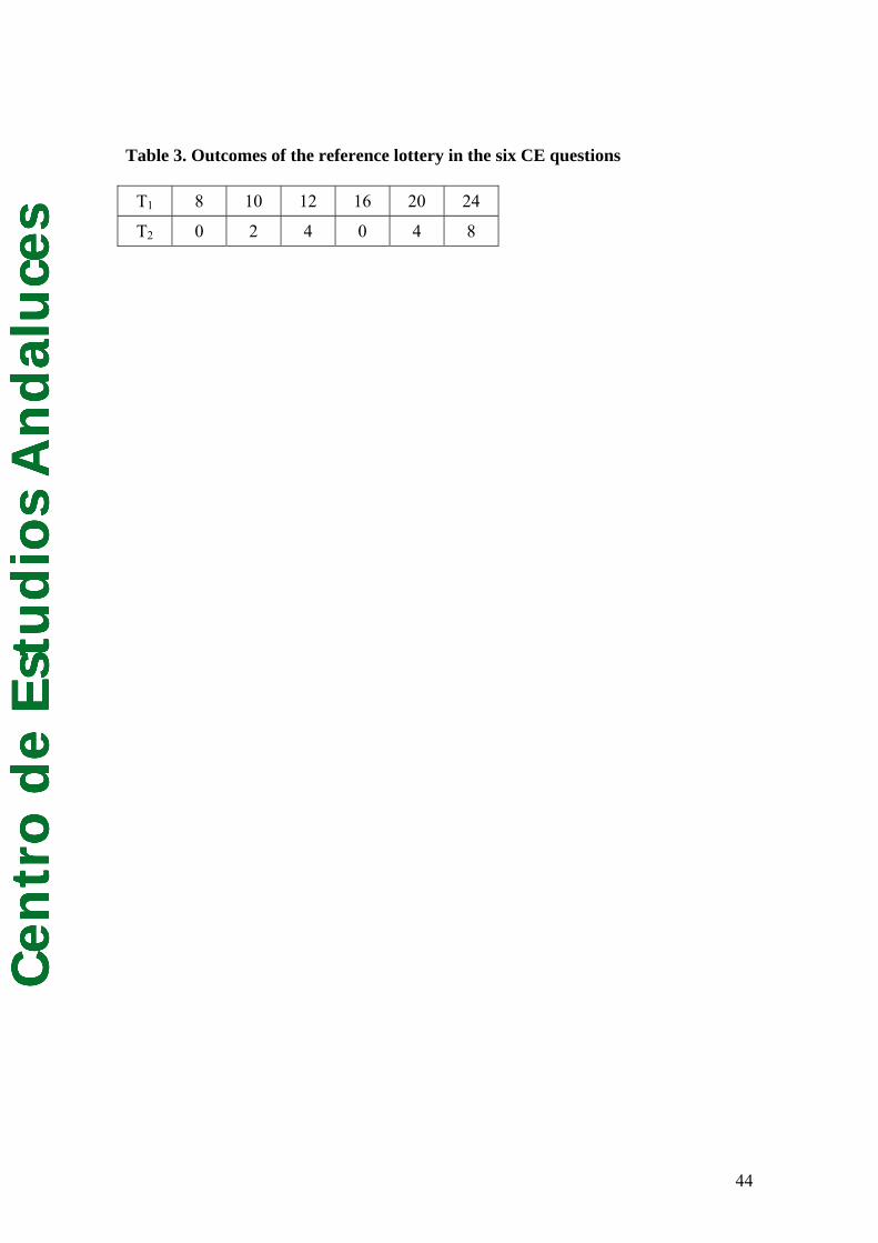
Cen

tro

de

Est

ud

ios

An

dal

uce

s

Table 3. Outcomes of the reference lottery in the six CE questions

T1 8 10 12 16 20 24

T2 0 2 4 0 4 8

44

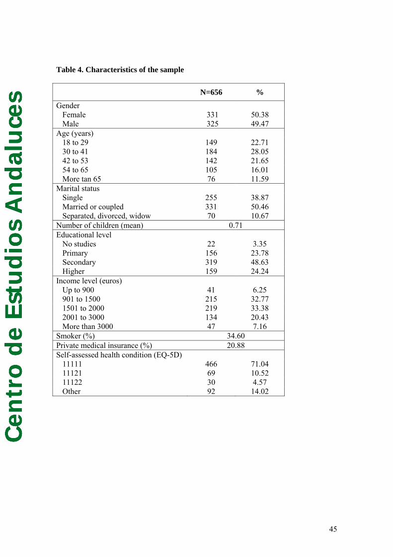
Cen

tro

de

Est

ud

ios

An

dal

uce

s

Table 4. Characteristics of the sample

N=656 %

Gender Female 331 50.38 Male 325 49.47

Age (years) 18 to 29 149 22.71 30 to 41 184 28.05 42 to 53 142 21.65 54 to 65 105 16.01 More tan 65 76 11.59

Marital status Single 255 38.87 Married or coupled 331 50.46 Separated, divorced, widow 70 10.67

Number of children (mean) 0.71 Educational level

No studies 22 3.35 Primary 156 23.78 Secondary 319 48.63 Higher 159 24.24

Income level (euros) Up to 900 41 6.25 901 to 1500 215 32.77 1501 to 2000 219 33.38 2001 to 3000 134 20.43 More than 3000 47 7.16

Smoker (%) 34.60 Private medical insurance (%) 20.88 Self-assessed health condition (EQ-5D)

11111 466 71.04 11121 69 10.52 11122 30 4.57 Other 92 14.02

45

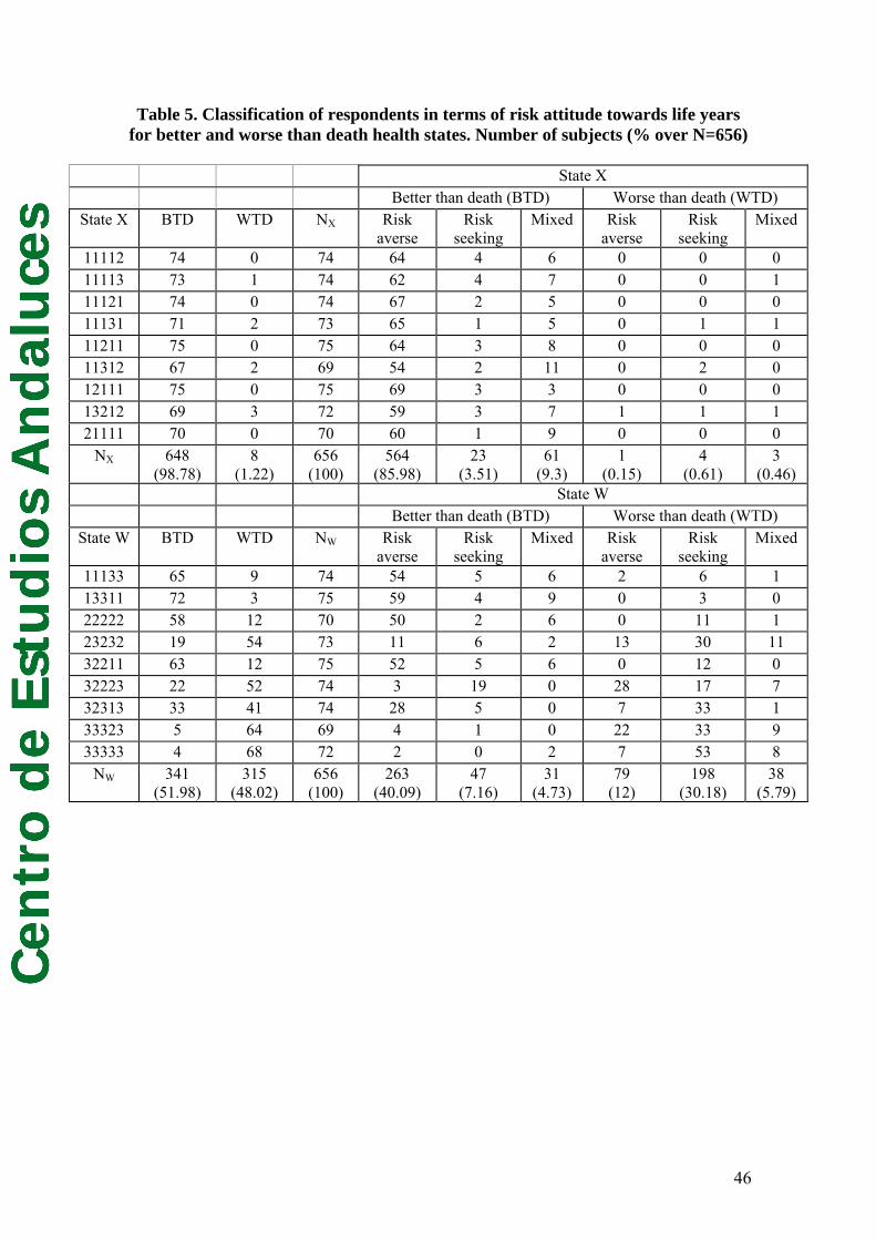
Cen

tro

de

Est

ud

ios

An

dal

uce

sTable 5. Classification of respondents in terms of risk attitude towards life years

for better and worse than death health states. Number of subjects (% over N=656)

State X Better than death (BTD) Worse than death (WTD)

State X BTD WTD NX Risk averse

Risk seeking

Mixed Risk averse

Risk seeking

Mixed

11112 74 0 74 64 4 6 0 0 0 11113 73 1 74 62 4 7 0 0 1 11121 74 0 74 67 2 5 0 0 0 11131 71 2 73 65 1 5 0 1 1 11211 75 0 75 64 3 8 0 0 0 11312 67 2 69 54 2 11 0 2 0 12111 75 0 75 69 3 3 0 0 0 13212 69 3 72 59 3 7 1 1 1 21111 70 0 70 60 1 9 0 0 0

NX 648 (98.78)

8 (1.22)

656 (100)

564 (85.98)

23 (3.51)

61 (9.3)

1 (0.15)

4 (0.61)

3 (0.46)

State W Better than death (BTD) Worse than death (WTD)

State W BTD WTD NW Risk averse

Risk seeking

Mixed Risk averse

Risk seeking

Mixed

11133 65 9 74 54 5 6 2 6 1 13311 72 3 75 59 4 9 0 3 0 22222 58 12 70 50 2 6 0 11 1 23232 19 54 73 11 6 2 13 30 11 32211 63 12 75 52 5 6 0 12 0 32223 22 52 74 3 19 0 28 17 7 32313 33 41 74 28 5 0 7 33 1 33323 5 64 69 4 1 0 22 33 9 33333 4 68 72 2 0 2 7 53 8

NW 341 (51.98)

315 (48.02)

656 (100)

263 (40.09)

47 (7.16)

31 (4.73)

79 (12)

198 (30.18)

38 (5.79)

46

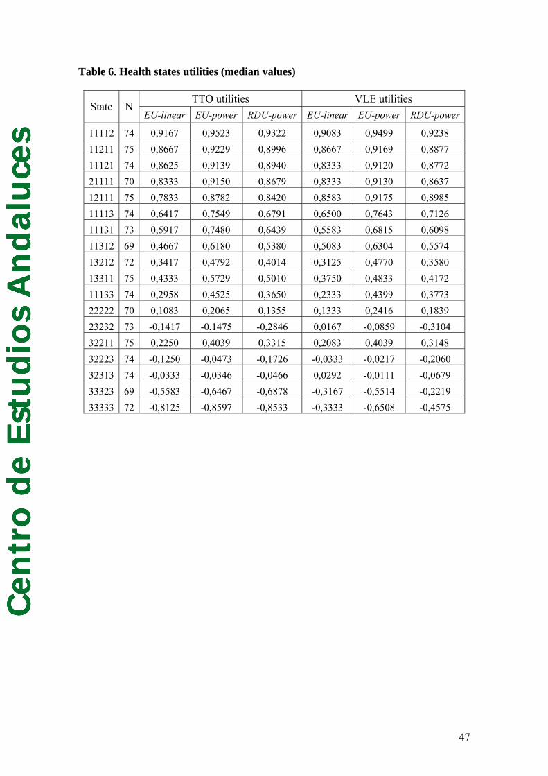
Cen

tro

de

Est

ud

ios

An

dal

uce

sTable 6. Health states utilities (median values)

TTO utilities VLE utilities State N

EU-linear EU-power RDU-power EU-linear EU-power RDU-power

11112 74 0,9167 0,9523 0,9322 0,9083 0,9499 0,9238 11211 75 0,8667 0,9229 0,8996 0,8667 0,9169 0,8877 11121 74 0,8625 0,9139 0,8940 0,8333 0,9120 0,8772 21111 70 0,8333 0,9150 0,8679 0,8333 0,9130 0,8637 12111 75 0,7833 0,8782 0,8420 0,8583 0,9175 0,8985 11113 74 0,6417 0,7549 0,6791 0,6500 0,7643 0,7126 11131 73 0,5917 0,7480 0,6439 0,5583 0,6815 0,6098 11312 69 0,4667 0,6180 0,5380 0,5083 0,6304 0,5574 13212 72 0,3417 0,4792 0,4014 0,3125 0,4770 0,3580 13311 75 0,4333 0,5729 0,5010 0,3750 0,4833 0,4172 11133 74 0,2958 0,4525 0,3650 0,2333 0,4399 0,3773 22222 70 0,1083 0,2065 0,1355 0,1333 0,2416 0,1839 23232 73 -0,1417 -0,1475 -0,2846 0,0167 -0,0859 -0,3104 32211 75 0,2250 0,4039 0,3315 0,2083 0,4039 0,3148 32223 74 -0,1250 -0,0473 -0,1726 -0,0333 -0,0217 -0,2060 32313 74 -0,0333 -0,0346 -0,0466 0,0292 -0,0111 -0,0679 33323 69 -0,5583 -0,6467 -0,6878 -0,3167 -0,5514 -0,2219 33333 72 -0,8125 -0,8597 -0,8533 -0,3333 -0,6508 -0,4575

47

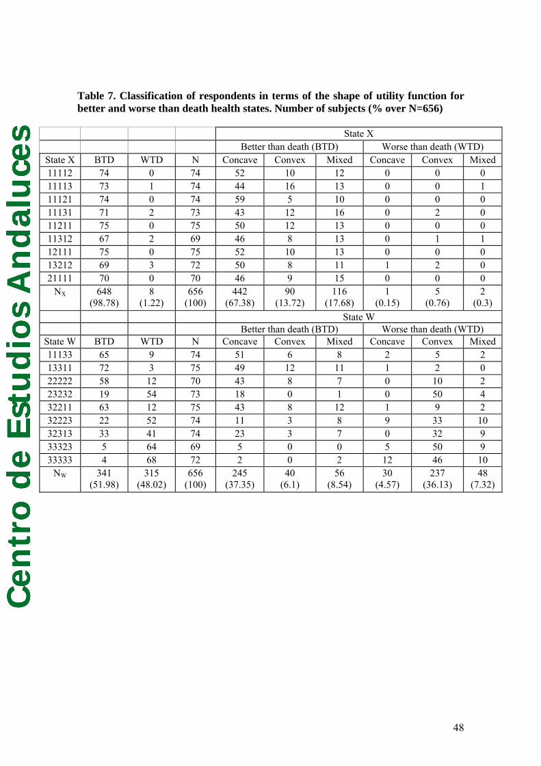
Cen

tro

de

Est

ud

ios

An

dal

uce

s

Table 7. Classification of respondents in terms of the shape of utility function for better and worse than death health states. Number of subjects (% over N=656) State X Better than death (BTD) Worse than death (WTD)

State X BTD WTD N Concave Convex Mixed Concave Convex Mixed 11112 74 0 74 52 10 12 0 0 0 11113 73 1 74 44 16 13 0 0 1 11121 74 0 74 59 5 10 0 0 0 11131 71 2 73 43 12 16 0 2 0 11211 75 0 75 50 12 13 0 0 0 11312 67 2 69 46 8 13 0 1 1 12111 75 0 75 52 10 13 0 0 0 13212 69 3 72 50 8 11 1 2 0 21111 70 0 70 46 9 15 0 0 0

NX 648 (98.78)

8 (1.22)

656 (100)

442 (67.38)

90 (13.72)

116 (17.68)

1 (0.15)

5 (0.76)

2 (0.3)

State W Better than death (BTD) Worse than death (WTD)

State W BTD WTD N Concave Convex Mixed Concave Convex Mixed 11133 65 9 74 51 6 8 2 5 2 13311 72 3 75 49 12 11 1 2 0 22222 58 12 70 43 8 7 0 10 2 23232 19 54 73 18 0 1 0 50 4 32211 63 12 75 43 8 12 1 9 2 32223 22 52 74 11 3 8 9 33 10 32313 33 41 74 23 3 7 0 32 9 33323 5 64 69 5 0 0 5 50 9 33333 4 68 72 2 0 2 12 46 10

NW 341 (51.98)

315 (48.02)

656 (100)

245 (37.35)

40 (6.1)

56 (8.54)

30 (4.57)

237 (36.13)

48 (7.32)

48