The psychometric function: I. Fitting, sampling, and … several goodness-of-fit tests. Using Monte Carlo simulations, we deal with two specific difficulties that arise when fitting

Perception & Psychophysics2001, 63 (8), 1293-1313

The performance of an observer on a psychophysicaltask is typically summarized by reporting one or moreresponse thresholds—stimulus intensities required to pro-duce a given level of performance—and by characteriza-tion of the rate at which performance improves with in-creasing stimulus intensity. These measures are derivedfrom a psychometric function, which describes the depen-dence of an observer’s performance on some physical as-pect of the stimulus: One example might be the relation be-tween the contrast of a visual stimulus and the observer’sability to detect it.

Fitting psychometric functions is a variant of the moregeneral problem of modeling data. Modeling data is a three-step process. First, a model is chosen, and the parametersare adjusted to minimize the appropriate error metric orloss function. Second, error estimates of the parametersare derived, and third, the goodness of fit between themodel and the data is assessed. This paper is concerned

with the first and the third of these steps, parameter esti-mation and goodness-of-fit assessment. Our companionpaper (Wichmann & Hill, 2001) deals with the second stepand illustrates how to derive reliable error estimates onthe fitted parameters. Together, the two papers providean integrated approach to fitting psychometric functions,evaluating goodness of fit, and obtaining confidence in-tervals for parameters, thresholds, and slopes, avoidingthe known sources of potential error.

This paper is divided into two major subsections, fittingpsychometric functions and goodness of fit. Each subsec-tion itself is again subdivided into two main parts: first, anintroduction to the issue, and second, a set of simulationsaddressing the issue raised in the respective introduction.

NOTATION

We adhere mainly to the typographic conventions fre-quently encountered in statistical texts (Collett, 1991;Dobson, 1990; Efron & Tibshirani, 1993). Variables are de-noted by uppercase italic letters, and observed values aredenoted by the corresponding lowercase letters—for ex-ample, y is a realization of the random variable Y. Greekletters are used for parameters, and a circumflex for esti-mates; thus, parameter b is estimated by b. Vectors aredenoted by boldface lowercase letters, and matrices byboldface italic uppercase letters. The ith element of a vec-tor x is denoted by xi. The probability density function ofthe random variable Y (or the probability distribution if Yis discrete) with q as the vector of parameters of the dis-tribution is written as p( y;q). Simulated data sets (repli-cations) are indicated by an asterisk—for example, ai* is

1293 Copyright 2001 Psychonomic Society, Inc.

This research was supported by a Wellcome Trust Mathematical Bi-ology Studentship, a Jubilee Scholarship from St. Hugh’s College, Ox-ford, and a Fellowship by Examination from Magdalen College, Oxford,to F.A.W. and by a grant from the Christopher Welch Trust Fund and aMaplethorpe Scholarship from St. Hugh’s College, Oxford, to N.J.H. Weare indebted to Andrew Derrington, Karl Gegenfurtner, and Bruce Hen-ning for helpful comments and suggestions. This paper benefited con-siderably from conscientious peer review, and we thank our reviewersDavid Foster, Stan Klein, Marjorie Leek, and Bernhard Treutwein forhelping us improve our manuscript. Software implementing the methodsdescribed in this paper is available written in MATLAB; contact F.A.W. atthe address provided or see http://users.ox.ac.uk/~sruoxfor/psychofit /.Correspondence concerning this article should be addressed to F. A. Wich-mann, Max-Planck-Institut für Biologische Kybernetik, Spemannstraße38, D-72076 Tübingen, Germany (e-mail: felix@tuebingen. mpg.de).

The psychometric function:I. Fitting, sampling, and goodness of fit

FELIX A. WICHMANN and N. JEREMY HILLUniversity of Oxford, Oxford, England

The psychometric function relates an observer’s performance to an independent variable, usually somephysical quantity of a stimulus in a psychophysical task. This paper, together with its companion paper(Wichmann & Hill, 2001), describes an integrated approach to (1) fitting psychometric functions, (2) as-sessing the goodness of fit, and (3) providing confidence intervals for the function’s parameters and otherestimates derived from them, for the purposes of hypothesis testing. The present paper deals with the firsttwo topics, describing a constrained maximum-likelihood method of parameter estimation and develop-ing several goodness-of-fit tests. Using Monte Carlo simulations, we deal with two specific difficulties thatarise when fitting functions to psychophysical data. First, we note that human observers are prone tostimulus-independent errors (or lapses). We show that failure to account for this can lead to serious bi-ases in estimates of the psychometric function’s parameters and illustrate how the problem may be over-come. Second, we note that psychophysical data sets are usually rather small by the standards requiredby most of the commonly applied statistical tests. We demonstrate the potential errors of applying tradi-tional c 2 methods to psychophysical data and advocate use of Monte Carlo resampling techniques thatdo not rely on asymptotic theory. We have made available the software to implement our methods.

1294 WICHMANN AND HILL

the value of a in the ith Monte Carlo simulation. The nthquantile of a distribution x is denoted by x(n).

FITTING PSYCHOMETRIC FUNCTIONS

BackgroundTo determine a threshold, it is common practice to fit a

two-parameter function to the data and to compute the in-verse of that function for the desired performance level.The slope of the fitted function at a given level of perfor-mance serves as a measure of the change in performancewith changing stimulus intensity. Statistical estimation ofparameters is routine in data modeling (Dobson, 1990;McCullagh & Nelder, 1989): In the context of fitting psy-chometric functions, probit analysis (Finney, 1952 , 1971)and a maximum-likelihood search method described byWatson (1979) are most commonly employed. Recently,Treutwein and Strasburger (1999) have described a con-strained generalized maximum-likelihood procedure thatis similar in some respects to the method we advocate inthis paper.

In the following, we review the application of maximum-likelihood estimators in fitting psychometric functionsand the use of Bayesian priors in constraining the fit ac-cording to the assumptions of one’s model. In particular,we illustrate how an often disregarded feature of psy-chophysical data—namely, the fact that observers some-times make stimulus-independent lapses—can introducesignificant biases into the parameter estimates. The ad-verse effect of nonstationary observer behavior (of whichlapses are an example) on maximum-likelihood parameterestimates has been noted previously (Harvey, 1986; Swan-son & Birch, 1992; Treutwein, 1995; cf. Treutwein & Stras-burger, 1999). We show that the biases depend heavily onthe sampling scheme chosen (by which we mean the pat-tern of stimulus values at which samples are taken) but thatit can be corrected, at minimal cost in terms of parametervariability, by the introduction of an additional free buthighly constrained parameter determining, in effect, theupper bound of the psychometric function.

The psychometric function. Psychophysical data aretaken by sampling an observer’s performance on a psycho-physical task at a number of different stimulus levels. Inthe method of constant stimuli, each sample point is takenin the form of a block of experimental trials at the samestimulus level. In this paper, K denotes the number of suchblocks or datapoints. A data set can thus be described bythree vectors, each of length K: x will denote the stimuluslevels or intensities of the blocks, n the number of trialsor observations in each block, and y the observer’s per-formance, expressed as a proportion of correct responses(in forced-choice paradigms) or positive responses (insingle-interval or yes/no experiments). We will use N torefer to the total number of experimental trials, N 5 åni.

To model the process underlying experimental data, itis common to assume the number of correct responses yiniin a given block i to be the sum of random samples from a

Bernoulli process with a probability of success pi. A modelmust then provide a psychometric function y(x), whichspecifies the relationship between the underlying proba-bility of a correct (or positive) response p and the stimulusintensity x. A frequently used general form is

(1)

The shape of the curve is determined by the parameters {a,b, g, l}, to which we shall refer collectively by using theparameter vector qq, and by the choice of a two-parameterfunction F, which is typically a sigmoid function, such asthe Weibull, logistic, cumulative Gaussian, or Gumbel dis-tribution.1

The function F is usually chosen to have range [0, 1], [0,1), or (0,1). Thus, the parameter g gives the lower bound ofy(x;qq), which can be interpreted as the base rate of per-formance in the absence of a signal. In forced-choiceparadigms (n-AFC), this will usually be fixed at the rec-iprocal of the number of alternatives per trial. In yes/noparadigms, it is often taken as corresponding to the guessrate, which will depend on the observer and experimentalconditions. In this paper, we will use examples from onlythe 2AFC paradigm, and thus assume g to be fixed at .5.The upper bound of the curve—that is, the performancelevel for an arbitrarily large stimulus signal—is given by1 2 l. For yes/no experiments, l corresponds to the missrate, and in n-AFC experiments, it is, similarly, a reflec-tion of the rate at which observers lapse, responding in-correctly regardless of stimulus intensity.2 Between thetwo bounds, the shape of the curve is determined by a andb. The exact meaning of a and b depends on the form ofthe function chosen for F, but together they will determinetwo independent attributes of the psychometric function:its displacement along the abscissa and its slope.

We shall assume that F describes the performance ofthe underlying psychological mechanism of interest. Al-tough it is important to have correct values for g and l , thevalues themselves are of secondary scientific interest,since they arise from the stimulus-independent mecha-nisms of guessing and lapsing. Therefore, when we referto the threshold and slope of a psychometric function, wemean the inverse of F at some particular performancelevel as a measure of displacement and the gradient of Fat that point as a measure of slope. Where we do not spec-ify a performance level, the value .5 should be assumed:Thus threshold refers F -1

0.5 to and slope refers to F¢ eval-uated at F -1

0.5. In our 2AFC examples, these values willroughly correspond to the stimulus value and slope at the75% correct point, although the exact predicted perfor-mance will be affected slightly by the (small) value of l .

Maximum-likelihood estimation. Likelihood maxi-mization is a frequently used technique for parameter es-timation (Collett, 1991; Dobson, 1990; McCullagh & Nel-der, 1989). For our problem, provided that the values of yare assumed to have been generated by Bernoulli pro-cesses, it is straightforward to compute a likelihood valuefor a particular set of parameters qq, given the observed

y a b g l g g l a b( ; , , , ) ( ) ( ; , ).x F x= + - -1

PSYCHOMETRIC FUNCTION I 1295

values y. The likelihood function L(qq;y) is the same as theprobability function p(y|qq) (i.e. , the probability of havingobtained data y given hypothetical generating parametersqq)—note, however, the reversal of order in the notation,to stress that once the data have been gathered, y is fixed,and qq is the variable. The maximum-likelihood estimatorqq of qq is simply that set of parameters for which the like-lihood value is largest: L(qq;y) $ L(qq;y) for all qq. Since thelogarithm is a monotonic function, the log-likelihoodfunction l(qq;y) 5 l(qq;y) is also maximized by the same es-timator qq, and this frequently proves to be easier to max-imize numerically. For our situation, it is given by

(2)

In principle, qq can be found by solving for the points atwhich the derivative of l(qq;y) with respect to all the pa-rameters is zero: This gives a set of local minima and max-ima, from which the global maximum of l(qq;y) is selected.For most practical applications, however, qq is determinedby iterative methods, maximizing those terms of Equation 2that depend on qq. Our implementation of log-likelihoodmaximization uses the multidimensional Nelder–Meadsimplex search algorithm,3 a description of which can befound in chapter 10 of Press, Teukolsky, Vetterling, andFlannery (1992).

Bayesian priors. It is sometimes possible that themaximum-likelihood estimate qq contains parameter val-ues that are either nonsensical or inappropriate. For exam-ple, it can happen that the best fit to a particular data sethas a negative value for l , which is uninterpretable as alapse rate and implies that an observer’s performance canexceed 100% correct—clearly nonsensical psychologically,even though l(qq; y) may be a real value for the particularstimulus values in the data set.

It may also happen that the data are best fit by a pa-rameter set containing a large l (greater than .06, for ex-ample). A large l is interpreted to mean that the observermakes a large proportion of incorrect responses no matterhow great the stimulus intensity—in most normal psycho-physical situations, this means that the experiment wasnot performed properly and that the data are invalid. If theobserver genuinely has a lapse rate greater than .06, he orshe requires extra encouragement or, possibly, replace-ment. However, misleadingly large l values may also befitted when the observer performs well, but there are nosamples at high performance values.

In both cases, it would be better for the fitting algorithmto return parameter vectors that may have a lower log-likelihood than the global maximum but that contain morerealistic values. Bayesian priors provide a mechanism forconstraining parameters within realistic ranges, based onthe experimenter’s prior beliefs about the likelihood ofparticular values. A prior is simply a relative probability

distribution W(qq), specified in advance, which weights thelikelihood calculation during fitting: The fitting processtherefore maximizes W(qq)L(qq;y) or log W(qq) 1 l(qq;y),instead of the unweighted metrics.

The exact form of W(qq) is to be chosen by the experi-menter, given the experimental context. The ideal choicefor W(l) would be the distribution of rates of stimulus-independent error for the current observer on the currenttask. Generally, however, one has not enough data to esti-mate this distribution. For the simulations reported in thispaper, we chose W(l) 5 1 for 0 # l # .06; otherwise,W(l) 5 04—that is, we set a limit of .06 on l , and weightsmaller values equally with a flat prior.5,6 For data analy-sis, we generally do not constrain the other parameters,except to limit them to values for which y(x;qq) is real.

Avoiding bias caused by observers’ lapses. In stud-ies in which sigmoid functions are fitted to psychophys-ical data, particularly where the data come from forced-choice paradigms, it is common for experimenters to fixl 5 0, so that the upper bound of y(x;qq) is always 1.0.Thus, it is assumed that observers make no stimulus-independent errors. Unfortunately, maximum-likelihoodparameter estimation as described above is extremely sen-sitive to such stimulus-independent errors, with a conse-quent bias in threshold and slope estimates (Harvey, 1986;Swanson & Birch, 1992).

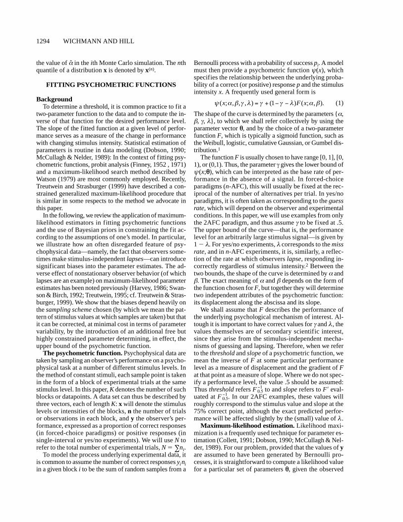
Figure 1 illustrates the problem. The dark circles indi-cate the proportion of correct responses made by an ob-server in six blocks of trials in a 2AFC visual detectiontask. Each datapoint represents 50 trials, except for the lastone, at stimulus value 3.5, which represents 49 trials: Theobserver still has one trial to perform to complete theblock. If we were to stop here and fit a Weibull functionto the data, we would obtain the curve plotted as a darksolid line. Whether or not l is fixed at 0 during the fit, themaximum-likelihood parameter estimates are the same:{a5 1.573, b 5 4.360, l 5 0}. Now suppose that, on the50th trial of the last block, the observer blinks and missesthe stimulus, is consequently forced to guess, and happensto guess wrongly. The new position of the datapoint atstimulus value 3.5 is shown by the light triangle: It hasdropped from 1.00 to .98 proportion correct.

The solid light curve shows the results of fitting a two-parameter psychometric function (i.e. , allowing a and bto vary, but keeping l fixed at 0). The new fitted param-eters are {a 5 2.604, b 5 2.191}. Note that the slope ofthe fitted function has dropped dramatically in the spaceof one trial—in fact, from a value of 1.045 to 0.560. If weallow l to vary in our new fit, however, the effect on pa-rameters is slight—{a 5 1.543, b 5 4.347, l 5 .014}—and thus, there is little change in slope: dF/dx evaluated atx 5 F -1

0.5 is 1.062.The misestimation of parameters shown in Figure 1 is

a direct consequence of the binomial log-likelihood errormetric because of its sensitivity to errors at high levels ofpredicted performance:7 since y(x;qq) ® 1, so, in the thirdterm of Equation 2, (1 2 yi)ni log[1 2 y(xi;qq)] ® 2¥ un-

l yn

y ny n x

y n x

i

i ii i i

i

K

i i i

( ; ) log log ( ; )

( log ; .

q q

q

=æ

èç

ö

ø÷ +

+ -( ) - ( )[ ]=å y

y1

1 1


less the coefficient (1 2 yi)ni is 0. Since yi represents ob-served proportion correct, the coefficient is 0 as long asperformance is perfect. However, as soon as the observerlapses, the coefficient becomes nonzero and allows thelarge negative log term to influence the log-likelihood sum,reflecting the fact that observed proportions less than 1are extremely unlikely to have been generated from anexpected value that is very close to 1. Log-likelihood canbe raised by lowering the predicted value at the last stim-ulus value, y(3.5,qq). Given that l is fixed at 0, the upperasymptote is fixed at 1.0; hence, the best the fitting algo-rithm can do in our example to lower y(3.5,qq) is to makethe psychometric function shallower.

Judging the fit by eye, it does not appear to captureaccurately the rate at which performance improves withstimulus intensity. (Proper Monte Carlo assessments ofgoodness of fit are described later in this paper.)

The problem can be cured by allowing l to take a non-zero value, which can be interpreted to reflect our beliefas experimenters that observers can lapse and that, there-fore, in some cases, their performance might fall below100% despite arbitrarily large stimulus values. To obtainthe optimum value of l and, hence, the most accurate es-timates for the other parameters, we allow l to vary in themaximum-likelihood search. However, it is constrainedwithin the narrow range [0,.06], reflecting our beliefs con-cerning its likely values8 (see the previous section, on Baye-sian priors).

The example of Figure 1 might appear exaggerated; thedistortion in slope was obtained by placing the last sam-

ple point (at which the lapse occurred) at a comparativelyhigh stimulus value relative to the rest of the data set. Thequestion remains: How serious are the consequences of as-suming a fixed l for sampling schemes one might readilyemploy in psychophysical research?

SimulationsTo test this, we conducted Monte Carlo simulations; six-

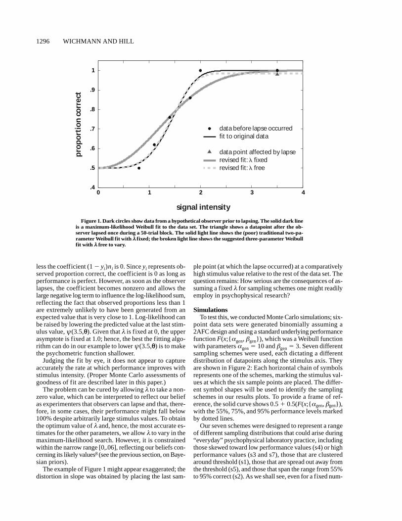
point data sets were generated binomially assuming a2AFC design and using a standard underlying performancefunction F(x;{agen, bgen}), which was a Weibull functionwith parameters agen 5 10 and bgen 5 3. Seven differentsampling schemes were used, each dictating a differentdistribution of datapoints along the stimulus axis. Theyare shown in Figure 2: Each horizontal chain of symbolsrepresents one of the schemes, marking the stimulus val-ues at which the six sample points are placed. The differ-ent symbol shapes will be used to identify the samplingschemes in our results plots. To provide a frame of ref-erence, the solid curve shows 0.5 1 0.5(F(x;{agen, bgen}),with the 55%, 75%, and 95% performance levels markedby dotted lines.

Our seven schemes were designed to represent a rangeof different sampling distributions that could arise during“everyday” psychophysical laboratory practice, includingthose skewed toward low performance values (s4) or highperformance values (s3 and s7), those that are clusteredaround threshold (s1), those that are spread out away fromthe threshold (s5), and those that span the range from 55%to 95% correct (s2). As we shall see, even for a fixed num-

0 1 2 3 4.4

.5

.6

.7

.8

.9

1

signal intensity

pro

po

rtio

n c

orr

ect

data before lapse occurredfit to original data

data point affected by lapserevised fit: l fixedrevised fit: l free

Figure 1. Dark circles show data from a hypothetical observer prior to lapsing. The solid dark lineis a maximum-likelihood Weibull fit to the data set. The triangle shows a datapoint after the ob-server lapsed once during a 50-trial block. The solid light line shows the (poor) traditional two-pa-rameter Weibull fit with ll fixed; the broken light line shows the suggested three-parameter Weibullfit with ll free to vary.


ber of sample points and a f ixed number of trials perpoint, biases in parameter estimation and goodness-of-fitassessment (this paper) as well as the width of confidenceintervals (companion paper, Wichmann & Hill, 2001), alldepend heavily on the distribution of stimulus values x.

The number of datapoints was always 6, but the num-ber of observations per point was 20, 40, 80, or 160. Thismeant that the total number of observations N could be120, 240, 480, or 960.

We also varied the rate at which our simulated observerlapsed. Our model for the processes involved in a singletrial was as follows: For every trial at stimulus value xi, theobserver’s probability of correct response ygen(xi) is givenby 0.5 1 0.5F(xi;{agen, bgen}), except that there is a cer-tain small probability that something goes wrong, in whichcase ygen(xi) is instead set at a constant value k. The valueof k would depend on exactly what goes wrong. Perhapsthe observer suffers a loss of attention, misses the stimu-lus, and is forced to guess; then, k would be .5, reflectingthe probability of the guess’ being correct. Alternatively,lapses might occur because the observer fails to respondwithin a specified response interval, which the experi-menter interprets as an incorrect response, in which casek 5 0. Or perhaps k has an intermediate value that re-flects a probabilistic combination of these two events and/or other potential mishaps. In any case, provided we as-sume that such events are independent, that their probabil-ity of occurrence is constant throughout a single block oftrials, and that k is constant, the simulated observer’s over-all performance on a block is binomially distributed, withan underlying probability that can be expressed with Equa-

tion 1—it is easy to show that variations in k or in theprobability of a mishap are described by a change in l . Weshall use lgen to denote the generating function’s l param-eter, possible values for which were 0, .01, .02, .03, .04,and .05.

To generate each data set, then, we chose (1) a samplingscheme, which gave us the vector of stimulus values x,(2) a value for N, which was divided equally among the el-ements of the vector n denoting the number of observa-tions in each block, and (3) a value for lgen, which was as-sumed to have the same value for all blocks of the dataset.9 We then obtained the simulated performance vectory: For each block i, the proportion of correct responses yiwas obtained by finding the proportion of a set of ni ran-dom numbers10 that were less than or equal to ygen(xi). Amaximum-likelihood fit was performed on the data setdescribed by x, y, and n, to obtain estimated parametersa, b , and l. There were two fitting regimes: one in whichl was fixed at 0, and one in which it was allowed to varybut was constrained within the range [0, .06]. Thus, therewere 336 conditions: 7 sampling schemes 3 6 values forlgen 3 4 values for N 3 2 fitting regimes. Each conditionwas replicated 2,000 times, using a new randomly gen-erated data set, for a total of 672,000 simulations overall,requiring 3.024 3 108 simulated 2AFC trials.

Simulation results: 1. Accuracy. We are interested inmeasuring the accuracy of the two fitting regimes in es-timating the threshold and slope, whose true values aregiven by the stimulus value and gradient of F(x;{agen,bgen}) at the point at which F(x;{agen, bgen}) 5 0.5. Thetrue values are 8.85 and 0.118, respectively—that is, it is

4 5 7 10 12 15 17 200

.1

.2

.3

.4

.5

.6

.7

.8

.9

1

signal intensity

pro

po

rtio

n c

orr

ect

s7

s6

s5

s4

s3

s2

s1

Figure 2. A two-alternative forced-choice Weibull psychometric function with parameter vectorqq 5 {10, 3, .5, 0} on semilogarithmic coordinates. The rows of symbols below the curve mark the xvalues of the seven different sampling schemes used throughout the remainder of the paper.


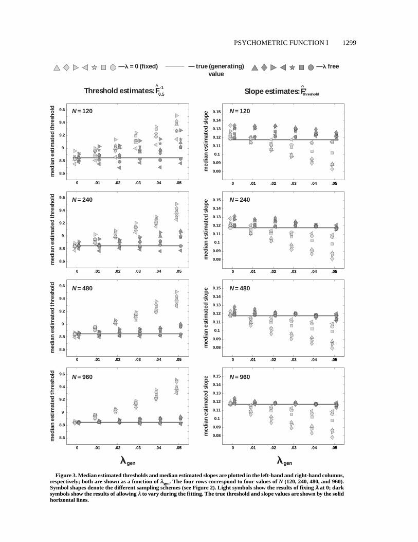
F(8.85;{10, 3}) 5 0.5 and F¢(8.85;{10, 3}) 5 0.118. Fromeach simulation, we use the estimated parameters to ob-tain the threshold and slope of F(x;{a, b}). The mediansof the distributions of 2,000 thresholds and slopes fromeach condition are plotted in Figure 3. The left-hand col-umn plots median estimated threshold, and the right-hand column plots median estimated slope, both as afunction of lgen. The four rows correspond to the fourvalues of N: The total number of observations increasesdown the page. Symbol shape denotes sampling schemeas per Figure 2. Light symbols show the results of fixingl at 0, and dark symbols show the results of allowing lto vary during the fitting process. The true threshold andslope values (i.e. , those obtained from the generating func-tion) are shown by the solid horizontal lines.

The first thing to notice about Figure 3 is that, in all theplots, there is an increasing bias in some of the samplingschemes’ median estimates as lgen increases. Some sam-pling schemes are relatively unaffected by the bias. Byusing the shape of the symbols to refer back to Figure 2,it can be seen that the schemes that are affected to thegreatest extent (s3, s5, s6, and s7) are those containingsample points at which F(x,{agen, bgen}) . 0.9, whereasthe others (s1, s2, and s4) contain no such points and areaffected to a lesser degree. This is not surprising, bearingin mind the foregoing discussion of Equation 1: Bias ismost likely where high performance is expected.

Generally, then, the variable-l regime performs betterthan the fixed-l regime in terms of bias. The one excep-tion to this can be seen in the plot of median slope esti-mates for N 5 120 (20 observations per point): Here,there is a slight upward bias in the variable-l estimates,an effect that varies according to sampling scheme but thatis relatively unaffected by the value of lgen. In fact, forlgen # .02, the downward bias from the fixed-l fits issmaller, or at least no larger, than the upward bias fromfits with variable l. Note, however, that an increase in Nto 240 or more improves the variable-l estimates, reduc-ing the bias and bringing the medians from the differentsampling schemes together. The variable-l f ittingscheme is essentially unbiased for N $ 480, independentof the sampling scheme chosen. By contrast, the value ofN appears to have little or no effect on the absolute sizeof the bias inherent in the susceptible fixed-l schemes.

Simulation results: 2. Precision. In Figure 3, the biasseems fairly small for threshold measurements (maximally,about 8% of our stimulus range when the fixed-l fittingregime is used or about 4% when l is allowed to vary).For slopes, only the fixed-l regime is affected, but the ef-fect, expressed as a percentage, is more pronounced (upto 30% underestimation of gradient).

However, note that however large or small the bias ap-pears when expressed in terms of stimulus units, knowl-edge about an estimator’s precision is required in order toassess the severity of the bias. Severity in this case meansthe extent to which our estimation procedure leads us tomake errors in hypothesis testing: finding differences be-tween experimental conditions where none exist (Type I

errors) or failing to find them when they do exist (Type II).The bias of an estimator must thus be evaluated relativeto its variability. A frequently applied rule of thumb is thata good estimator should be biased by less than 25% of itsstandard deviation (Efron & Tibshirani, 1993).

The variability of estimates in the context of fitting psy-chometric functions is the topic of our companion paper(Wichmann & Hill, 2001), in which we shall see that one’schosen sampling scheme and the value of N both have aprofound effect on confidence interval width. For now, andwithout going into too much detail, we are merely inter-ested in knowing how our decision to employ a fixed-lor a variable-l regime affects variability (precision) for thevarious sampling schemes and to use this information toassess the severity of bias.

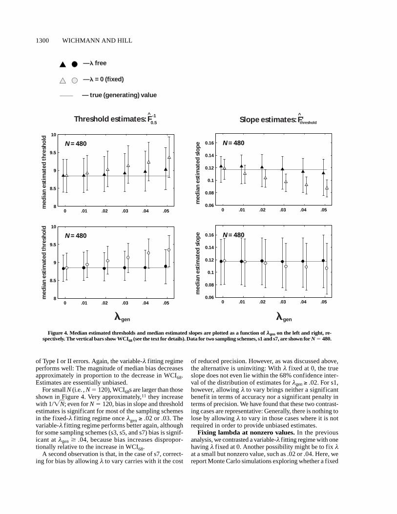
Figure 4 shows two illustrative cases, plotting resultsfor two contrasting schemes at N 5 480. The upper pairof plots shows the s7 sampling scheme, which, as we haveseen, is highly susceptible to bias when l is fixed at 0and observers lapse. The lower pair shows s1, which wehave already found to be comparatively resistant to bias.As before, thresholds are plotted on the left and slopeson the right, light symbols represent the fixed-l fittingregime, dark symbols represent the variable-l fittingregime, and the true values are again shown as solid hor-izontal lines. Each symbol’s position represents the me-dian estimate from the 2,000 fits at that point, so they areexactly the same as the upward triangles and circles inthe N 5 480 plots of Figure 3. The vertical bars show theinterval between the 16th and the 84th percentiles ofeach distribution (these limits were chosen because theygive an interval with coverage of .68, which would be ap-proximately the same as the mean plus or minus onestandard deviation (SD) if the distributions were Gauss-ian). We shall use WCI68 as shorthand for width of the68% confidence interval in the following.

Applying the rule of thumb mentioned above(bias # 0.25 SD), bias in the fixed-l condition in thethreshold estimate is significant for lgen . .02, for bothsampling schemes. The slope estimate of the fixed-l fit-ting regime and the sampling scheme s7 is significantlybiased once observers lapse—that is, for lgen $ .01. It isinteresting to see that even the threshold estimates of s1,with all sample points at p , .8, are significantly biasedby lapses. The slight bias found with the variable-l fittingregime, however, is not significant in any of the casesstudied.

We can expect the variance of the distribution of esti-mates to be a function of N—the WCI68 gets smaller withincreasing N. Given that the absolute magnitude of biasstays the same for the fixed-l fitting regime, however, bias willbecome more problematic with increasing N: For N 5 960,the bias in threshold and slope estimates is significantfor all sampling schemes and virtually all nonzero lapserates. Frequently, the true (generating) value is not evenwithin the 95% confidence interval. Increasing the num-ber of observations by using the fixed-l fitting regime,contrary to what one might expect, increases the likelihood


lgenlgen

med

ian

est

imat

ed s

lop

e

med

ian

est

imat

ed t

hre

sho

ld

med

ian

est

imat

ed s

lop

e

med

ian

est

imat

ed t

hre

sho

ld

med

ian

est

imat

ed s

lop

e

med

ian

est

imat

ed t

hre

sho

ld

med

ian

est

imat

ed s

lop

e

med

ian

est

imat

ed t

hre

sho

ld

—l free—l = 0 (fixed) — true (generating)value

Threshold estimates: F^ -1

0.5 Slope estimates: F'^

threshold

0 .01 .02 .03 .04 .05

0.08

0.09

0.1

0.11

0.12

0.13

0.14

0.15

0 .01 .02 .03 .04 .05

0.08

0.09

0.1

0.11

0.12

0.13

0.14

0.15

0 .01 .02 .03 .04 .05

0.08

0.09

0.1

0.11

0.12

0.13

0.14

0.15

0 .01 .02 .03 .04 .05

0.08

0.09

0.1

0.11

0.12

0.13

0.14

0.15

0 .01 .02 .03 .04 .05

8.6

8.8

9

9.2

9.4

9.6

0 .01 .02 .03 .04 .05

8.6

8.8

9

9.2

9.4

9.6

0 .01 .02 .03 .04 .05

8.6

8.8

9

9.2

9.4

9.6

0 .01 .02 .03 .04 .05

8.6

8.8

9

9.2

9.4

9.6

N = 120

N = 240

N = 480

N = 960

N = 120

N = 240

N = 480

N = 960

Figure 3. Median estimated thresholds and median estimated slopes are plotted in the left-hand and right-hand columns,respectively; both are shown as a function of llgen. The four rows correspond to four values of N (120, 240, 480, and 960).Symbol shapes denote the different sampling schemes (see Figure 2). Light symbols show the results of fixing ll at 0; darksymbols show the results of allowing ll to vary during the fitting. The true threshold and slope values are shown by the solidhorizontal lines.


of Type I or II errors. Again, the variable-l fitting regimeperforms well: The magnitude of median bias decreasesapproximately in proportion to the decrease in WCI68.Estimates are essentially unbiased.

For small N (i.e. , N 5 120), WCI68s are larger than thoseshown in Figure 4. Very approximately,11 they increasewith 1/ÏNw; even for N 5 120, bias in slope and thresholdestimates is significant for most of the sampling schemesin the fixed-l fitting regime once lgen ³ .02 or .03. Thevariable-l fitting regime performs better again, althoughfor some sampling schemes (s3, s5, and s7) bias is signif-icant at lgen $ .04, because bias increases dispropor-tionally relative to the increase in WCI68.

A second observation is that, in the case of s7, correct-ing for bias by allowing l to vary carries with it the cost

of reduced precision. However, as was discussed above,the alternative is uninviting: With l fixed at 0, the trueslope does not even lie within the 68% confidence inter-val of the distribution of estimates for lgen ³ .02. For s1,however, allowing l to vary brings neither a significantbenefit in terms of accuracy nor a significant penalty interms of precision. We have found that these two contrast-ing cases are representative: Generally, there is nothing tolose by allowing l to vary in those cases where it is notrequired in order to provide unbiased estimates.

Fixing lambda at nonzero values. In the previousanalysis, we contrasted a variable-l fitting regime with onehaving l fixed at 0. Another possibility might be to fix lat a small but nonzero value, such as .02 or .04. Here, wereport Monte Carlo simulations exploring whether a fixed

0 .01 .02 .03 .04 .058

8.5

9

9.5

10

N = 480

0 .01 .02 .03 .04 .058

8.5

9

9.5

10

N = 480

0 .01 .02 .03 .04 .050.06

0.08

0.1

0.12

0.14

0.16 N = 480

0 .01 .02 .03 .04 .050.06

0.08

0.1

0.12

0.14

0.16 N = 480

lgenlgen

med

ian

est

imat

ed s

lop

e

med

ian

est

imat

ed t

hre

sho

ld

med

ian

est

imat

ed s

lop

e

med

ian

est

imat

ed t

hre

sho

ld

—l free

—l = 0 (fixed)

— true (generating) value



threshold

Figure 4. Median estimated thresholds and median estimated slopes are plotted as a function of llgen on the left and right, re-spectively. The vertical bars show WCI68 (see the text for details). Data for two sampling schemes, s1 and s7, are shown for N 5 480.


small value of l overcomes the problems of bias whileretaining the desirable property of (slightly) increasedprecision relative to the variable-l fitting regime.

Simulations were repeated as before, except that l waseither free to vary or fixed at .01, .02, .03, .04, and .05,covering the whole range of lgen. (A total of 2,016,000simulations, requiring 9.072 3 109 simulated 2AFC trials.)

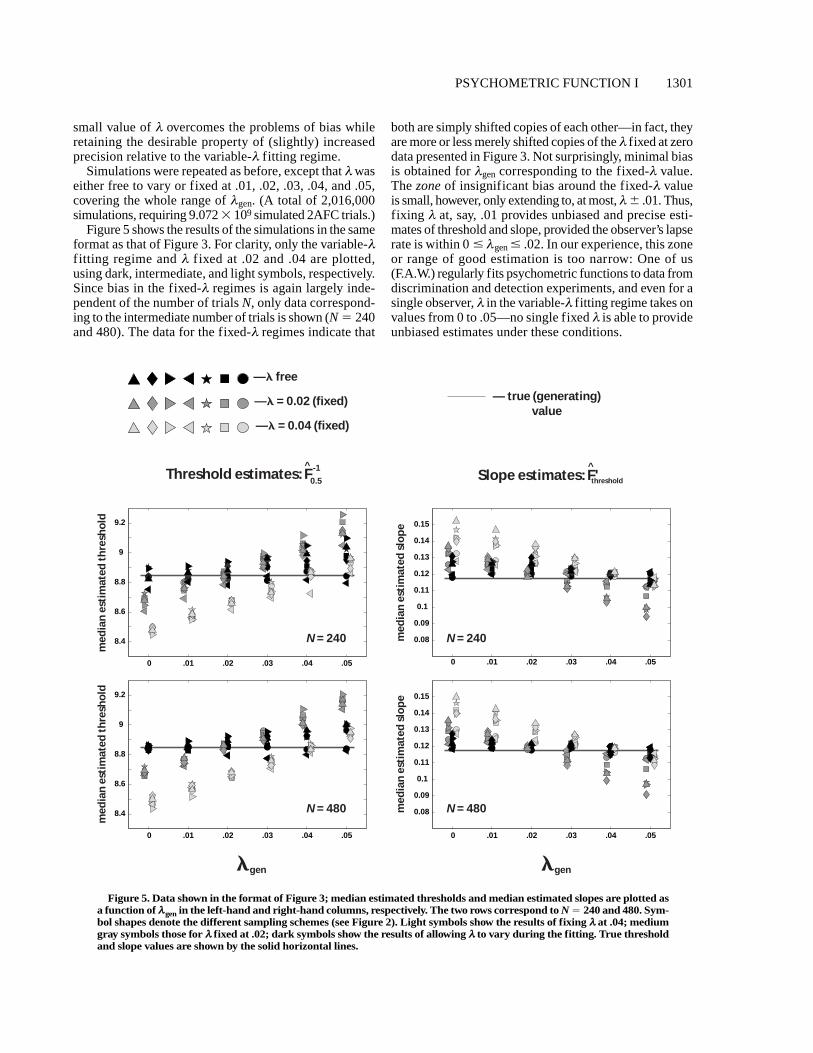
Figure 5 shows the results of the simulations in the sameformat as that of Figure 3. For clarity, only the variable-lfitting regime and l fixed at .02 and .04 are plotted,using dark, intermediate, and light symbols, respectively.Since bias in the fixed-l regimes is again largely inde-pendent of the number of trials N, only data correspond-ing to the intermediate number of trials is shown (N 5 240and 480). The data for the fixed-l regimes indicate that

both are simply shifted copies of each other—in fact, theyare more or less merely shifted copies of the l fixed at zerodata presented in Figure 3. Not surprisingly, minimal biasis obtained for lgen corresponding to the fixed-l value.The zone of insignificant bias around the fixed-l valueis small, however, only extending to, at most, l 6 .01. Thus,fixing l at, say, .01 provides unbiased and precise esti-mates of threshold and slope, provided the observer’s lapserate is within 0 # lgen # .02. In our experience, this zoneor range of good estimation is too narrow: One of us(F.A.W.) regularly fits psychometric functions to data fromdiscrimination and detection experiments, and even for asingle observer, l in the variable-l fitting regime takes onvalues from 0 to .05—no single fixed l is able to provideunbiased estimates under these conditions.

Figure 5. Data shown in the format of Figure 3; median estimated thresholds and median estimated slopes are plotted asa function of llgen in the left-hand and right-hand columns, respectively. The two rows correspond to N 5 240 and 480. Sym-bol shapes denote the different sampling schemes (see Figure 2). Light symbols show the results of fixing ll at .04; mediumgray symbols those for ll fixed at .02; dark symbols show the results of allowing ll to vary during the fitting. True thresholdand slope values are shown by the solid horizontal lines.

0 .01 .02 .03 .04 .05

8.4

8.6

8.8

9

9.2

0 .01 .02 .03 .04 .05

0.08

0.09

0.1

0.11

0.12

0.13

0.14

0.15

0 .01 .02 .03 .04 .05

8.4

8.6

8.8

9

9.2

0 .01 .02 .03 .04 .05

0.08

0.09

0.1

0.11

0.12

0.13

0.14

0.15

lgenlgen

med

ian

est

imat

ed s

lop

e

med

ian

est

imat

ed t

hre

sho

ld

med

ian

est

imat

ed s

lop

e

med

ian

est

imat

ed t

hre

sho

ld

— true (generating)value



threshold

—l free

—l = 0.04 (fixed)

—l = 0.02 (fixed)

N = 240N = 240

N = 480 N = 480


Discussion and SummaryCould bias be avoided simply by choosing a sampling

scheme in which performance close to 100% is not ex-pected? Since one never knows the psychometric functionexactly in advance before choosing where to sample per-formance, it would be difficult to avoid high performance,even if one were to want to do so. Also, there is good rea-son to choose to sample at high performance values: Pre-cisely because data at these levels have a greater influenceon the maximum-likelihood fit, they carry more informa-tion about the underlying function and thus allow more ef-ficient estimation. Accordingly, Figure 4 shows that theprecision of slope estimates is better for s7 than for s1 (cf.Lam, Mills, & Dubno, 1996). This issue is explored morefully in our companion paper (Wichmann & Hill, 2001). Fi-nally, even for those sampling schemes that contain no sam-ple points at performance levels above 80%, bias in thresh-old estimates was significant, particularly for large N.

Whether sampling deliberately or accidentally at highperformance levels, one must allow for the possibility thatobservers will perform at high rates and yet occasionallylapse: Otherwise, parameter estimates may become biasedwhen lapses occur. Thus, we recommend that varying las a third parameter be the method of choice for fittingpsychometric functions.

Fitting a tightly constrained l is intended as a heuristicto avoid bias in cases of nonstationary observer behavior.It is, as well, to note that the estimated parameter l is, ingeneral, not a very good estimator of a subject’s truelapse rate (this was also found by Treutwein & Stras-burger, 1999, and can be seen clearly in their Figures 7and 10). Lapses are rare events, so there will only be avery small number of lapsed trials per data set. Further-more, their directly measurable effect is small, so thatonly a small subset of the lapses that occur (those at highx values where performance is close to 100%) will affectthe maximum-likelihood estimation procedure; the restwill be lost in binomial noise. With such minute effectivesample sizes, it is hardly surprising that our estimates ofl per se are poor. However, we do not need to worry, be-cause as psychophysicists we are not interested in lapses:We are interested in thresholds and slopes, which are de-termined by the function F that reflects the underlyingmechanism. Therefore, we vary l not for its own sake, butpurely in order to free our threshold and slope estimatesfrom bias. This it accomplishes well, despite numericallyinaccurate l estimates. In our simulations, it works wellboth for sampling schemes with a fixed nonzero lgen andfor those with more random lapsing schemes (see note 9or our example shown in Figure 1).

In addition, our simulations have shown that N 5 120appears too small a number of trials to be able to obtain re-liable estimates of thresholds and slopes for some sam-pling schemes, even if the variable-l fitting regime is em-ployed. Similar conclusions were reached by O’Regan andHumbert (1989) for N 5 100 (K 5 10; cf. Leek, Hanna,

& Marshall, 1992; McKee, Klein, & Teller, 1985). This isfurther supported by the analysis of bootstrap sensitivityin our companion paper (Wichmann & Hill, 2001).

GOODNESS OF FIT

BackgroundAssessing goodness of fit is a necessary component of

any sound procedure for modeling data, and the impor-tance of such tests cannot be stressed enough, given thatfitted thresholds and slopes, as well as estimates of vari-ability (Wichmann & Hill, 2001), are usually of very lim-ited use if the data do not appear to have come from thehypothesized model. A common method of goodness-of-fit assessment is to calculate an error term or summarystatistic, which can be shown to be asymptotically dis-tributed according to c2—for example, Pearson X 2—andto compare the error term against the appropriate c2 dis-tribution. A problem arises, however, since psychophysicaldata tend to consist of small numbers of points and it is,hence, by no means certain that such tests are accurate. Apromising technique that offers a possible solution isMonte Carlo simulation, which being computationally in-tensive, has become practicable only in recent years withthe dramatic increase in desktop computing speeds. It ispotentially well suited to the analysis of psychophysicaldata, because its accuracy does not rely on large numbersof trials, as do methods derived from asymptotic theory(Hinkley, 1988). We show that for the typically small K andN used in psychophysical experiments, assessing good-ness of fit by comparing an empirically obtained statisticagainst its asymptotic distribution is not always reliable:The true small-sample distribution of the statistic is ofteninsufficiently well approximated by its asymptotic distri-bution. Thus, we advocate generation of the necessary dis-tributions by Monte Carlo simulation.

Lack of fit—that is, the failure of goodness of fit—mayresult from failure of one or more of the assumptions ofone’s model. First and foremost, lack of fit between themodel and the data could result from an inappropriatefunctional form for the model—in our case of fitting a psy-chometric function to a single data set, the chosen under-lying function F is significantly different from the true one.Second, our assumption that observer responses are bino-mial may be false: For example, there might be serial de-pendencies between trials within a single block. Third, theobserver’s psychometric function may be nonstationaryduring the course of the experiment, be it due to learn-ing or fatigue.

Usually, inappropriate models and violations of inde-pendence result in overdispersion or extra-binomial vari-ation: “bad fits” in which datapoints are significantly fur-ther from the fitted curve than was expected. Experimenterbias in data selection (e.g. , informal removal of outliers),on the other hand, could result in underdispersion: fits thatare “too good to be true,” in which datapoints are signifi-


cantly closer to the fitted curve than one might expect (suchdata sets are reported more frequently in the psychophysi-cal literature than one would hope12).

Typically, if goodness of fit of fitted psychometric func-tions is assessed at all, however, only overdispersion isconsidered. Of course, this method does not allow us todistinguish between different sources of overdispersion(wrong underlying function or violation of independence)and/or effects of learning. Furthermore, as we will show,models can be shown to be in error even if the summarystatistic indicates an acceptable fit.

In the following, we describe a set of goodness-of-fittests for psychometric functions (and parametric modelsin general). Most of them rely on different analyses of theresidual differences between data and fit (the sum ofsquares of which constitutes the popular summary statis-tics) and on Monte Carlo generation of the statistic’s dis-tribution, against which to assess lack of fit. Finally, weshow how a simple application of the jackknife resamplingtechnique can be used to identify so-called influentialobservations—that is, individual points in a data set thatexert undue influence on the final parameter set. Jackknifetechniques can also provide an objective means of iden-tifying outliers.

Assessing overdispersion. Summary statistics measurecloseness of the data set as a whole to the fitted function.Assessing closeness is intimately linked to the fitting pro-cedure itself: Selecting the appropriate error metric forfitting implies that the relevant currency within which tomeasure closeness has been identified. How good or badthe fit is should thus be assessed in the same currency.

In maximum-likelihood parameter estimation, the pa-rameter vector qq returned by the fitting routine is suchthat L(qq; y) $ L(qq; y) for all qq. Thus, whatever error met-ric, Z, is used to assess goodness of fit,

(3)

should hold for all qq.Deviance. The log-likelihood ratio, or deviance, is a

monotonic transformation of likelihood and therefore ful-fills the criterion set out in Equation 3. Hence, it is com-monly used in the context of generalized linear models(Collett, 1991; Dobson, 1990; McCullagh & Nelder, 1989).

Deviance, D, is defined as

(4)

where L(qqmax;y) denotes the likelihood of the saturatedmodel—that is, a model with no residual error betweenempirical data and model predictions. (qqmax denotes theparameter vector such that this holds and the number offree parameters in the saturated model is equal to the totalnumber of blocks of observations, K.) L(qq;y) is the likeli-hood of the best-fitting model; l(qqmax;y) and l(qq;y) de-note the logarithms of these quantities, respectively. Be-cause, by definition, l(qqmax;y) $ l(qq;y) for all qq, and

l(qqmax;y) is independent of qq (being purely a function ofthe data, y), deviance fulfills the criterion set out inEquation 3. From Equation 4 we see that deviance takesvalues from 0 (no residual error) to infinity (observeddata are impossible given model predictions).

For goodness-of-fit assessment of psychometric func-tions (binomial data), Equation 4 reduces to

(5)

( pi refers to the proportion correct predicted by the fittedmodel).

Deviance is used to assess goodness of fit, rather thanlikelihood or log-likelihood directly, because, for correctmodels, deviance for binomial data is asymptotically dis-tributed as c 2

K , where K denotes the number of data-points (blocks of trials).13 For derivation, see, for exam-ple, Dobson (1990, p. 57), McCullagh and Nelder (1989),and in particular, Collett (1991, sects. 3.8.1 and 3.8.2).Calculating D from one’s fit and comparing it with theappropriate c2 distribution, hence, allows simple good-ness-of-fit assessment, provided that the asymptotic ap-proximation to the (unknown) distribution of deviance isaccurate for one’s data set. The specific values of L(qq;y)or l(qq;y) or by themselves, on the other hand, are lessgenerally interpretable.

Pearson X 2. The Pearson X 2 test is widely used ingoodness-of-fit assessment of multinomial data; appliedto K blocks of binomial data, the statistic has the form

, (6)

with ni, yi, and pi as in Equation 5. Equation 6 can be in-terpreted as the sum of squared residuals (each residualbeing given by yi 2 pi), standardized by their variance,pi(1 - pi)ni

-1. Pearson X 2 is asymptotically distributed ac-cording to c 2 with K degrees of freedom, because the binomial distribution is asymptotically normal and c2

K isdefined as the distribution of the sum of K squared unit-variance normal deviates. Indeed, deviance D and Pear-son X 2 have the same asymptotic c2 distribution (but seenote 13).

There are two reasons why deviance is preferable toPearson X 2 for assessing goodness of fit after maximum-likelihood parameter estimation. First and foremost, for Pearson X 2, Equation 3 does not hold—that is, themaximum-likelihood parameter estimate qq will not gen-erally correspond to the set of parameters with the small-est error in the Pearson X 2 sense—that is, Pearson X 2 er-rors are the wrong currency (see the previous section,Assessing Overdispersion). Second, differences in deviancebetween two models of the same family—that is, betweenmodels where one model includes terms in addition tothose in the other—can be used to assess the significanceof the additional free parameters. Pearson X 2, on the other

Xn y p

p p

i i i

i ii

K2

2

1 1=

-( )-( )=

å

D n yy

pn y

y

pi i

i

ii i

i

ii

K

=æ

èç

ö

ø÷ + -( ) -

-

æ

èç

ö

ø÷

ìíî

üýþ=

å2 11

11

log log

DL

Ll l=

é

ëê

ù

ûú = -[ ]2 2log

( ; )

( ˆ; )( ; ) ( ˆ; ) ,max

maxqq

qqqq qq

y

yy y

Z Z( ˆ; ) ( ; )qq qqy y³


hand, cannot be used for such model comparisons (Collett,1991). This important issue will be expanded on when weintroduce an objective test of outlier identification.

SimulationsAs we have mentioned, both deviance for binomial data

and Pearson X 2 are only asymptotically distributed ac-cording to c2. In the case of Pearson X 2, the approximationto the c2 will be reasonably good once the K individual bi-nomial contributions to Pearson X2 are well approximatedby a normal—that is, as long as both ni pi $ 5 and ni(1 2pi) $ 5 (Hoel, 1984). Even for only moderately high p val-ues like .9, this already requires ni values of 50 or more,and p 5 .98 requires an ni of 250.

No such simple criterion exists for deviance, however.The approximation depends not only on K and N, but im-portantly, on the size of the individual ni and pi—it is dif-ficult to predict whether or not the approximation is suf-ficiently close for a particular data set. (see Collett, 1991,sect. 3.8.2). For binary data (i.e. , ni 5 1), deviance is noteven asymptotically distributed according to c2, and forsmall ni, the approximation can thus be very poor even ifK is large.

Monte-Carlo-based techniques are well suited to an-swering any question of the kind “what distribution ofvalues would we expect if . . .?” and, hence, offers a po-tential alternative to relying on the large-sample c2 approx-imation for assessing goodness of fit. The distribution ofdeviances is obtained in the following way. First, we gen-erate B data sets yi*, using the best-fitting psychometricfunction, y(x,qq), as the generating function. Then, for eachof the i 5 {1, . . . , B} generated data sets yi*, we calcu-late deviance Di*, using Equation 5, yielding the deviancedistribution D*. The distribution D* reflects the devianceswe should expect from an observer whose correct re-

sponses are binomially distributed with success proba-bility y(x,qq). A confidence interval for deviance can thenbe obtained by using the standard percentile method: D*(n)

denotes the 100 nth percentile of the distribution D* sothat, for example, the two-sided 95% confidence intervalis written as [D*(.025), D*(.975)].

Let Demp denote the deviance of our empirically ob-tained data set. If Demp . D*(.975), the agreement betweendata and fit is poor (overdispersion), and it is unlikely thatthe empirical data set was generated by the best-fittingpsychometric function, y(x,qq). y(x,qq) is, hence, not anadequate summary of the empirical data or the observer’sbehavior.

When using Monte Carlo methods to approximate thetrue deviance distribution D by D*, one requires a largevalue of B so that the approximation is good enough to betaken as the true or reference distribution—otherwise, wewould simply substitute errors arising from the inappro-priate use of an asymptotic distribution for numerical er-rors incurred by our simulations (Hämmerlin & Hoffmann,1991).

One way to see whether D* has indeed approached D isto look at the convergence of several of the quantiles ofD* with increasing B. For a large range of different val-ues of N, K, and ni, we found that for B $ 10,000, D* hasstabilized.14

Assessing errors in the asymptotic approximationto the deviance distribution. We have found, by a largeamount of trial-and-error exploration, that errors in thelarge-sample approximation to the deviance distributionare not predictable in a straightforward manner fromone’s chosen values of N, K, and x.

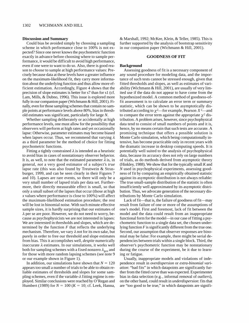
To illustrate this point, in this section we present six ex-amples in which the c2 approximation to the deviance dis-tribution fails in different ways. For each of the six ex-

Figure 6. Histograms of Monte-Carlo-generated deviance distributions D* (B 5 10,000). Both panelsshow distributions for N 5 300, K 5 6, and ni 5 50. The left-hand panel was generated from pgen 5 {.52,.56, .74, .94, .96, .98}; the right-hand panel was generated from pgen 5 {.63, .82, .89, .97, .99, .9999}. Thesolid dark line drawn with the histograms shows the c2

6 distribution (appropriately scaled).

0 5 10 15 20 25 300

500

1,000

1,500

0 5 10 15 20 250

400

800

1,200

DPRMS = 14.18DPmax = 18.42PF = 0PM = .596

deviance (D)

nu

mb

er p

er b

in

DPRMS = 4.63DPmax = 6.95PF = .011PM = 0

deviance (D)

nu

mb

er p

er b

in

N = 300, K = 6, ni = 50 N = 300, K = 6, ni = 50


amples, we conducted Monte Carlo simulations, eachusing B 5 10,000. Critically, for each set of simulations,a set of generating probabilities pgen was chosen: In a realexperiment, these values would be determined by the po-sitioning of one’s sample points x and the observer’s truepsychometric function ygen. The specific values of pgenin our simulations were chosen by us to demonstrate typ-ical ways in which the c2 approximation to the deviancedistribution fails: For the two examples shown in Figure 6,we change only pgen, keeping K and ni constant; for thetwo shown in Figure 7, ni was constant, and pgen coveredthe same range of values; Figure 8, finally, illustrates theeffect of changing ni while keeping pgen and K constant.

In order to assess the accuracy of the c2 approximationin all examples, we calculated the following four errorterms: (1) the rate at which using the c2 approximationwould have caused us to make Type I errors of rejection,rejecting simulated data sets that should not have beenrejected at the 5% level (we call this the false alarm rate,or PF), (2) the rate at which using the c2 approximationwould have caused us to make Type II errors of rejection,failing to reject a data set that the Monte Carlo distribu-tion D* indicated as rejectable at the 5% level (we call thisthe miss rate, PM), (3) the root-mean squared error DPRMSin cumulative probability estimate (CPE ), given by Equa-tion 9 (this is a measure of how different the Monte Carlodistribution D* and the appropriate c2 distribution are,on average), and (4) the maximal CPE error DPmax, givenby Equation 10, an indication of the maximal error in per-centile assignment that could result from using the c2 ap-proximation instead of the true D*.

The first two measures, PF and PM, are primarily usefulfor individual data sets. The latter two measures, DPRMSand DPmax, provide useful information in meta-analyses

(Schmidt, 1996), where models are assessed across sev-eral data sets. (In such analyses, we are interested in CPEerrors even if the deviance value of one particular dataset is not close to the tails of D: A systematic error inCPE in individual data sets might still cause errors of re-jection of the model as a whole, when all data sets areconsidered.)

In order to define DPRMS and DPmax, it is useful to in-troduce two additional terms, the Monte Carlo cumula-tive probability estimate CPEMC and the c2 cumulativeprobability estimate CPEc2. By CPEMC, we refer to

(7)

that is, the proportion of deviance values in D* smallerthan some reference value D of interest. Similarly,

(8)

provides the same information for the c2 distributionwith K degrees of freedom. The root-mean squared CPEerror DPRMS (average difference or error) is defined as

(9)

and the maximal CPE error DPmax (maximal difference orerror) is given by

(10)DP CPE D CPE D Ki imax max | ( ) ( , ) | .= -{ }100 2MC c

DP B CPE D CPE D KRMS i ii

B= -[ ]æ

èç

ö

ø÷

-

=å100 1 2

1

2MC ( ) ( , ) ,c

CPE D K x dx P DK

D

Kc c c22

0

2( , ) ( )= = £( )ò

CPE DD D

B

iMC ( ) =

£{ }+

#,

1

50 60 70 80 90 100 1100

200

400

600

800

1,000

240 260 280 300 320 340 360 3800

200

400

600

800

1,000

1,200

DPRMS = 55.16DPmax = 86.87PF = .899PM = 0

deviance (D)

nu

mb

er p

er b

in

DPRMS = 39.51DPmax = 56.32PF = .310PM = 0

deviance (D)

nu

mb

er p

er b

inN = 120, K = 60, ni = 2 N = 480, K = 240, ni = 2

Figure 7. Histograms of Monte-Carlo-generated deviance distributions D* (B 5 10,000). For both dis-tributions, pgen was uniformly distributed on the interval [.52, .85], and ni was equal to 2. The left-handpanel was generated using K 5 60 (N 5 120), and the solid dark line shows cc2

60 (appropriately scaled). Theright-hand panel’s distribution was generated using K 5 240 (N 5 480), and the solid dark line shows theappropriately scaled cc2

240 distribution.


Figure 6 illustrates two contrasting ways in which theapproximation can fail.15 The left-hand panel shows re-sults from the test in which the data sets were generatedfrom pgen 5 {.52, .56, .74, .94, .96, .98} with ni 5 50 ob-servations per sample point (K 5 6, N 5 300). Note thatthe c 2 approximation to the distribution is (slightly)shifted to the left. This results in DPRMS 5 4.63, DPmax 56.95, and a false alarm rate PF of 1.1%. The right-handpanel illustrates the results from very similar input condi-tions: As before, ni 5 50 observations per sample point (K5 6, N 5 300), but now pgen 5 {.63, .82, .89, .97, .99,.9999}. This time, the c2 approximation is shifted to theright, resulting in DPRMS 5 14.18, DPmax 5 18.42, and alarge miss rate: PM 5 59.6%.

Note that the reversal is the result of a comparativelysubtle change in the distribution of generating probabil-ities. These two cases illustrate the way in which asymp-totic theory may result in errors for sampling schemes thatmay occur in ordinary experimental settings, using themethod of constant stimuli. In our examples, the Type I er-rors (i.e. , erroneously rejecting a valid data set) of the left-hand panel may occur at a low rate, but they do occur. Thesubstantial Type II error rate (i.e. , accepting a data setwhose deviance is really too high and should thus be re-jected) shown on the right-hand panel, however, should because for some concern. In any case, the reversal of errortype, for the same values of K and ni, indicates that the typeof error is not predictable in any readily apparent way fromthe distribution of generating probabilities and the errorcannot be compensated for by a straightforward correction,such as a manipulation of the number of degrees of free-dom of the c2 approximation.

It is known that the large-sample approximation of thebinomial deviance distribution improves with an increase

in ni (Collett, 1991). In the above examples, ni was as largeas it is likely to get in most psychophysical experiments(ni 5 50), but substantial differences between the truedeviance distribution and its large-sample c2 approxima-tion were nonetheless observed. Increasingly frequently,psychometric functions are fitted to the raw data ob-tained from adaptive procedures (e.g. , Treutwein &Strasburger, 1999), with ni being considerably smaller.Figure 7 illustrates the profound discrepancy between thetrue deviance distribution and the c2 approximation underthese circumstances. For this set of simulations, ni wasequal to 2 for all i. The left-hand panel shows resultsfrom the test in which the data sets were generated fromK 5 60 sample points uniformly distributed over [.52,.85] (pgen 5 {.52, . . . , .85}), for a total of N 5 120 obser-vations. This results in DPRMS 5 39.51, DPmax 5 56.32,and a false alarm rate PF of 31.0 %. The right-hand panelillustrates the results from similar input conditions, ex-cept that K equaled 240 and N was thus 480. The c2 ap-proximation is even worse, with DPRMS 5 55.16, DPmax5 86.87, and a false alarm rate PF of 89.9%.

The data shown in Figure 7 clearly demonstrate that alarge number of observations N, by itself, is not a valid in-dicator of whether the c2 approximation is sufficientlygood to be useful for goodness-of-fit assessment.

After showing the effect of a change in pgen on the c2

approximation in Figure 6, and of K in Figure 7, Figure 8illustrates the effect of changing ni while keeping pgen andK constant: K 5 60 and pgen were uniformly distributedon the interval [.72, .99]. The left-hand panel shows resultsfrom the test in which the data sets were generated withni 5 2 observations per sample point (K 5 60, N 5 120).The c2 approximation to the distribution is shifted to theright, resulting in DPRMS 5 25.34, DPmax 5 34.92, and a

40 50 60 70 80 90 1000

200

400

600

800

1,000

1,200

30 40 50 60 70 80 900

200

400

600

800

1,000

DPRMS = 5.20DPmax = 8.50PF = 0PM = .702

deviance (D)

nu

mb

er p

er b

in

DPRMS = 25.34DPmax = 34.92PF = 0PM = .950

deviance (D)

nu

mb

er p

er b

inN = 120, K = 60, ni = 2 N = 240, K = 60, ni = 4

Figure 8. Histograms of Monte-Carlo-generated deviance distributions D* (B 5 10,000). For both distrib-utions, pgen was uniformly distributed on the interval [.72, .99], and K was equal to 60. The left-hand panel’sdistribution was generated using ni 5 2 (N 5 120); the right-hand panel’s distribution was generated usingni 5 4 (N 5 240). The solid dark line drawn with the histograms shows the cc2

60 distribution (appropriatelyscaled).


miss rate PM of 95%. The right-hand panel shows resultsfrom very similar generation conditions, except that ni 5 4(K 5 60, N 5 240). Note that, unlike in the other examplesintroduced so far, the mode of the distribution D* is notshifted relative to that of the c2

60 distribution, but that thedistribution is more leptokurtic (larger kurtosis or 4th-moment). DPRMS equals 5.20, DPmax equals 34.92, andthe miss rate PM is still a substantial 70.2%.

Comparing the left-hand panels of Figures 7 and 8 fur-ther points to the impact of p on the degree of the c2 ap-proximation to the deviance distribution: For constant N,K, and ni, we obtain either a substantial false alarm rate(PF 5 .31; Figure 7) or a substantial miss rate (PM 5 .95;Figure 8).

In general, we have found that very large errors in thec2 approximation are relatively rare for ni . 40, but theystill remain unpredictable (see Figure 6). For data sets withni , 20, on the other hand, substantial differences betweenthe true deviance distribution and its large-sample c2 ap-proximation are the norm, rather than the exception. Wethus feel that Monte-Carlo-based goodness-of-fit assess-ments should be preferred over c2-based methods for bi-nomial deviance.

Deviance residuals. Examination of residuals—theagreement between individual datapoints and the corre-sponding model prediction—is frequently suggested asbeing one of the most effective ways of identifying an in-correct model in linear and nonlinear regression (Collett,1991; Draper & Smith, 1981).

Given that deviance is the appropriate summary sta-tistic, it is sensible to base one’s further analyses on thedeviance residuals, d. Each deviance residual di is de-fined as the square root of the deviance value calculatedfor datapoint i in isolation, signed according to the direc-tion of the arithmetic residual yi 2 pi. For binomial data,this is

(11)

Note that

(12)

Viewed this way, the summary statistic deviance is thesum of the squared deviations between model and data; thedis are thus analogous to the normally distributed unit-variance deviations that constitute the c2 statistic.

Model checking. Over and above inspecting the resid-uals visually, one simple way of looking at the residualsis to calculate the correlation coefficient between theresiduals and the p values predicted by one’s model. Thisallows the identification of a systematic (linear) relationbetween deviance residuals d and model predictions p,which would suggest that the chosen functional form ofthe model is inappropriate—for psychometric functions,that presumably means that F is inappropriate.

Needless to say, a correlation coefficient of zero impliesneither that there is no systematic relationship betweenresiduals and the model prediction nor that the model cho-sen is correct; it simply means that whatever relation mightexist between residuals and model predictions, it is not alinear one.

Figure 9A shows data from a visual masking experi-ment with K 5 10 and ni 5 50, together with the best-fitting Weibull psychometric function (Wichmann, 1999).Figure 9B shows a histogram of D* for B 5 10,000 withthe scaled c2

10-PDF. The two arrows below the devianceaxis mark the two-sided 95% confidence interval [D*(.025),D*(.975)]. The deviance of the data set Demp is 8.34, andthe Monte Carlo cumulative probability estimate isCPEMC 5 .479. The summary statistic deviance, hence,does not indicate a lack of fit. Figure 9C shows the de-viance residuals d as a function of the model predictionp [p 5 y(x;qq) in this case, because we are using a fittedpsychometric function]. The correlation coefficient be-tween d and p is r 5 2.610. However, in order to deter-mine whether this correlation coefficient r is significant(of greater magnitude than expected by chance alone if ourchosen model was correct), we need to know the expecteddistribution r. For correct models, large samples, and con-tinuous data—that is, very large ni—one should expect thedistribution of the correlation coefficients to be a zero-mean Gaussian, but with a variance that itself is a functionof p and, hence, ultimately of one’s sampling scheme x.Asymptotic methods are, hence, of very limited applica-bility for this goodness-of-fit assessment.

Figure 9D shows a histogram of r*obtained by MonteCarlo simulation with B 5 10,000, again with arrowsmarking the two-sided 95% confidence interval [r*(.025),r*(.975)]. Confidence intervals for the correlation coeffi-cient are obtained in a manner analogous to the those ob-tained for deviance. First, we generate B simulated datasets yi*, using the best-fitting psychometric function asgenerating function. Then, for each synthetic data setyi*, we calculate the correlation coefficient ri* betweenthe deviance residuals di* calculated using Equation 11and the model predictions p 5 y(x;qq). From r*, one then ob-tains 95% confidence limits, using the appropriate quan-tile of the distribution.

In our example, a correlation of 2.610 is significant,the Monte Carlo cumulative probability estimate beingCPEMC(2.610) 5 .0015. (Note that the distribution isskewed and not centred on zero; a positive correlation ofthe same magnitude would still be within the 95% con-fidence interval.) Analyzing the correlation between de-viance residuals and model predictions thus allows us toreject the Weibull function as underlying function F forthe data shown in Figure 9A, even though the overall de-viance does not indicate a lack of fit.

Learning. Analysis of the deviance residuals d as afunction of temporal order can be used to show perceptuallearning, one type of nonstationary observer performance.The approach is equivalent to that described for modelchecking, except that the correlation coefficient of deviance

D dii

K

==å 2

1

.

d y p n yyp

n yyp

i i i i ii

ii i

i

i

= -( ) æèç

öø÷ + -( ) -

-æèç

öø÷

é

ëê

ù

ûúsgn log log .2 1

11


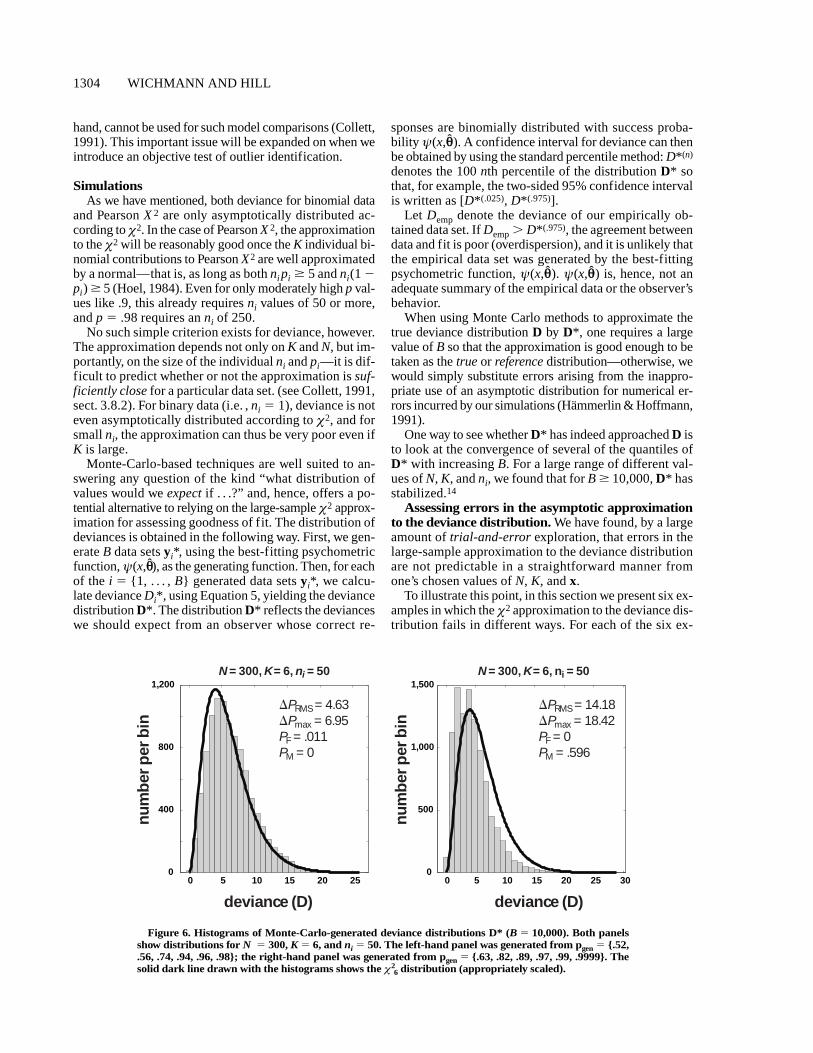
residuals is assessed as a function of the order in whichthe data were collected (often referred to as their index;Collett, 1991). Assuming that perceptual learning im-proves performance over time, one would expect the fit-ted psychometric function to be an average of the poorearlier performance and the better later performance.16

Deviance residuals should thus be negative for the firstfew datapoints and positive for the last ones. As a conse-quence, the correlation coefficient r of deviance residu-

als d against their indices (which we will denote by k) isexpected to be positive if the subject’s performance im-proved over time.

Figure 10A shows another data set from one of F.A.W.’sdiscrimination experiments; again, K 5 10 and ni 5 50,and the best-fitting Weibull psychometric function isshown with the raw data. Figure 10B shows a histogramof D* for B 5 10,000 with the scaled c2

10-PDF. The twoarrows below the deviance axis mark the two-sided 95%

deviancen

um

ber

per

bin

model prediction r

nu

mb

er p

er b

in

model prediction

dev

ian

ce r

esid

ual

s

signal contrast [%]

pro

po

rtio

n c

orr

ect

resp

on

ses

0.1 1 10

.6

.7

.8

.9

1

.5 K = 10, N = 500

Weibull psychometricfunction.u = {4.7; 1.98; 0.5; 0}

0 5 10 15 20 250

250

500

750

-0.8 -0.4 0 0.4 0.80

250

500

750

0.5 0.6 0.7 0.8 0.9 1

-1.5

-1

-0.5

0

0.5

1

1.5r = -.610

(A) (B)

(C)

(D)

DPRMS = 5.90DPmax = 9.30PF = 0PM = .340

Figure 9. (A) Raw data with N 5 500, K 5 10, and ni 5 50, together with the best-fitting Weibull psychometric functionyyfit with parameter vector qq 5 {4.7, 1.98, .5, 0} on semilogarithmic coordinates. (B) Histogram of Monte-Carlo-generateddeviance distribution D* (B 5 10,000) from yyfit. The solid vertical line marks the deviance of the empirical data set shownin panel A, Demp 5 8.34; the two arrows below the x-axis mark the two-sided 95% confidence interval [D*(.025), D*(.975)].(C) Deviance residuals d plotted as a function of model predictions p on linear coordinates. (D) Histogram of Monte-Carlo-generated correlation coefficients between d and p, r* (B 5 10,000). The solid vertical line marks the correlation coef-ficient between d and p 5 yyfit of the empirical data set shown in panel A, remp 5 2.610; the two arrows below the x-axismark the two-sided 95% confidence interval [r*(.025), r*(.975)].


confidence interval [D*(.025), D*(.975)]. The deviance of thedata set Demp is 16.97, the Monte Carlo cumulative prob-ability estimate CPEMC(16.97) being .914. The summarystatistic D does not indicate a lack of fit. Figure 10Cshows an index plot of the deviance residuals d. The cor-relation coefficient between d and k is r 5 .752, and thehistogram r* of shown in Figure 10D indicates that sucha high positive correlation is not expected by chancealone. Analysis of the deviance residuals against their

index is, hence, an objective means to identify percep-tual learning and, thus, reject the fit, even if the summarystatistic does not indicate a lack of fit.

Influential observations and outliers. Identificationof influential observations and outliers are additional re-quirements for comprehensive goodness-of-fit assess-ment.

The jackknife resampling technique. The jackknife isa resampling technique where K data sets, each of size

-1 -.8 -.6 -.4 -.2 0 .2 .4 .6 0.8 10

200

400

600

800

nu

mb

er p

er b

in

index

dev

ian

ce r

esid

ual

s

1 2 3 4 5 6 7 8 9 10-3

-2

-1

0

1

2

3

r = .752

1 10 100

.6

.7

.8

.9

1

signal contrast [%]

pro

po

rtio

n c

orr

ect

resp

on

ses

.5

K = 10, N = 500

Weibull psychometricfunction.u = {11.7; 0.89; 0.5; 0}

index r

nu

mb

er p

er b

in

(A) (b)

(C) (D)

1

2

3

4

56

7

8

9

10

0 5 10 15 20 25 300

250

500

750

deviance

DPRMS = 3.82DPmax = 5.77PF = 0.010PM = 0.000

(B)

Figure 10. (A) Raw data with N 5 500, K 5 10, and ni 5 50, together with the best-fitting Weibull psychometric function yyfitwith parameter vector qq 5 {11.7, 0.89, .5, 0} on semilogarithmic coordinates. The number next to each individual data point shows theindex ki of that data point. (B) Histogram of Monte-Carlo-generated deviance distribution D* (B 5 10,000) from yyfit. The solid ver-tical line marks the deviance of the empirical data set shown in panel A, Demp 5 16.97; the two arrows below the x-axis mark the two-sided 95% confidence interval [D*(.025), D*(.975)]. (C) Deviance residuals d plotted as a function of their index k. (D) Histogram ofMonte-Carlo-generated correlation coefficients between d and index k, r* (B 5 10,000). The solid vertical line marks the empiri-cal value of r for the data set shown in panel A, remp 5 .752; the two arrows below the x-axis mark the two-sided 95% confidenceinterval [r*(.025), r*(.975)].


K 2 1, are created from the original data set y by suc-cessively omitting one datapoint at a time. The jth jack-knife y(-j) data set is thus the same as y, but with the j thdatapoint of y omitted.17

Influential observations. To identify influential obser-vations, we apply the jackknife to the original data setand refit each jackknife data set y(-j); this yields K param-eter vectors qq(21), . . . , qq(-K). Influential observations arethose that exert an undue influence on one’s inferences—that is, on the estimated parameter vector qq—and to thisend, we compare qq(-1), …, qq(-K) with qq. If a jackknife pa-rameter set qq(-j) is significantly different from qq, the jthdatapoint is deemed an influential observation because itsinclusion in the data set alters the parameter vector sig-nificantly (from qq(-j) to qq).

Again, the question arises: What constitutes a signifi-cant difference between qq and qq(-j)? No general rules existto decide at which point qq(-j) and qq are significantly dif-ferent, but we suggest that one should be wary of one’ssampling scheme x if any one or several of the parametersets qq(-j) are outside the 95% confidence interval of qq. Ourcompanion paper describes a parametric bootstrap methodto obtain such confidence intervals for the parameters qq.Usually, identifying influential observations implies thatmore data need to be collected, at or around the influentialdatapoint(s).

Outliers. Like the test for influential observations, thisobjective procedure to detect outliers employs the jack-knife resampling technique. (Testing for outliers is some-times referred to as test of discordancy; Collett, 1991.) Thetest is based on a desirable property of deviance—namely,its nestedness: Deviance can be used to compare differ-ent models for binomial data as long as they are membersof the same family. Suppose a model M1 is a special caseof model M2 (M1 is “nested within” M2), so M1 has fewerfree parameters than M2. We denote the degrees of free-dom of the models by v1 and v2, respectively. Let the de-viance of model M1 be D1 and of M2 be D2. Then, the dif-ference in deviance, D1 2 D2, has an approximate c 2

distribution with v1 2 v2 degrees of freedom. This ap-proximation to the c2 distribution is usually very goodeven if each individual distribution, D1 or D2, is not reli-ably approximated by a c2 distribution (Collett, 1991); in-deed, D1 2 D2, has an approximate c2 distribution withv1 2 v2 degrees of freedom, even for binary data, despitethe fact that, for binary data, deviance is not even asymp-totically distributed according to c2 (Collett, 1991). Thisproperty makes this particular test of discordancy applic-able to (small-sample) psychophysical data sets.

To test for outliers, we again denote the original data setby y and its deviance by D. In the terminology of the pre-ceding paragraph, the fitted psychometric function y(x;qq)corresponds to model M1. Then, the jackknife is appliedto y, and each jackknife data set y(-j) is refit to give K pa-rameter vectors qq(-1), . . . , qq(-K), from which to calculate de-viance, yielding D(-1), . . . , D(-K ). For each of the K jack-

knife parameter vectors qq(-j), an alternative model M2 forthe (complete) original data set y is constructed as

(13)

Setting z equal to yj 2 y (x;qq(-j)), the deviance of M2 equalsD(-j), because the jth datapoint, dropped during the jack-knife, is perfectly fit by M2 owing to the addition of a ded-icated free parameter, z.

To decide whether the reduction in deviance, D 2 D(-j),is significant, we compare it against the c2 distribution withone degree of freedom, because v1 2 v2 5 1. Choosing aone-sided 99% confidence interval, M2 is a better modelthan M1 if D 2 D(-j) > 6.63, because CPEc2(6.63) 5 .99.Obtaining a significant reduction in deviance for data sety(-j) implies that the jth datapoint is so far away from theoriginal fit y(x;qq) that the addition of a dedicated pa-rameter z, whose sole function is to fit the j th datapoint,reduces overall deviance significantly. Datapoint j is thusvery likely an outlier, and as in the case of influential ob-servations, the best strategy generally is to gather addi-tional data at stimulus intensity xj, before more radicalsteps, such as removal of yj from one’s data set, are con-sidered.

DiscussionIn the preceding sections, we introduced statistical tests

to identify the following: first, inappropriate choice of F;second, perceptual learning; third, an objective test toidentify influential observations; and finally, an objectivetest to identify outliers. The histograms shown in Figures9D and 10D show the respective distributions r* to beskewed and not centered on zero. Unlike our summary sta-tistic D, where a large-sample approximation for binomialdata with ni > 1 exists even if its applicability is sometimeslimited, neither of the correlation coefficient statistics hasa distribution for which even a roughly correct asymptoticapproximation can easily be found for the K, N, and x typ-ically used in psychophysical experiments. Monte Carlomethods are thus without substitute for these statistics.

Figures 9 and 10 also provide another good demonstra-tion of our warnings concerning the c2 approximation ofdeviance. It is interesting to note that for both data sets,the MCS deviance histograms shown in Figures 9B and10B, when compared against the asymptotic c2 distribu-tions, have considerable DPRMS values of 3.8 and 5.9, withDPmax 5 5.8 and 9.3, respectively. Furthermore, the missrate in Figure 9B is very high (PM 5 .34). This is despitea comparatively large number of trials in total and perblock (N 5 500, ni 5 50), for both data sets. Further-more, whereas the c2 is shifted toward higher deviancesin Figure 9B, it is shifted toward lower deviance valuesin Figure 10B. This again illustrates the complex inter-action between deviance and p.

Mpi

xj

xi

xj

pi

xj

xi

xj

2:

( , ˆ( )

)

( , ˆ( )

).

= - + =

= - ¹ìíï

îïy z

y

qq

qq

if

if


SUMMARY AND CONCLUSIONS

In this paper, we have given an account of the proce-dures we use to estimate the parameters of psychometricfunctions and derive estimates of thresholds and slopes.An essential part of the fitting procedure is an assessmentof goodness of fit, in order to validate our estimates.

We have described a constrained maximum-likelihoodalgorithm for fitting three-parameter psychometric func-tions to psychophysical data. The third parameter, whichspecifies the upper asymptote of the curve, is highly con-strained, but it can be shown to be essential for avoidingbias in cases where observers make stimulus-independenterrors, or lapses. In our laboratory, we have found that thelapse rate for trained observers is typically between 0%and 5%, which is enough to bias parameter estimates sig-nificantly.

We have also described several goodness-of-fit statis-tics, all of which rely on resampling techniques to gen-erate accurate approximations to their respective distri-bution functions or to test for influential observations andoutliers. Fortunately, the recent sharp increase in com-puter processing speeds has made it possible to fulfillthis computationally expensive demand. Assessing good-ness of fit is necessary in order to ensure that our esti-mates of thresholds and slopes, and their variability, aregenerated from a plausible model for the data and toidentify problems with the data themselves, be they dueto learning, to uneven sampling (resulting in influentialobservations), or to outliers.

Together with our companion paper (Wichmann &Hill, 2001), we cover the three central aspects of model-ing experimental data: parameter estimation, obtainingerror estimates on these parameters, and assessing good-ness of fit between model and data.

REFERENCES

Collett, D. (1991). Modeling binary data. New York: Chapman &Hall/CRC.

Dobson, A. J. (1990). Introduction to generalized linear models. Lon-don: Chapman & Hall.

Draper, N. R., & Smith, H. (1981). Applied regression analysis. NewYork: Wiley.

Efron, B. (1979). Bootstrap methods: Another look at the jackknife.Annals of Statistics, 7, 1-26.

Efron, B. (1982). The jackknife, the bootstrap and other resamplingplans (CBMS-NSF Regional Conference Series in Applied Mathe-matics). Philadelphia: Society for Industrial and Applied Mathematics.

Efron, B., & Gong, G. (1983). A leisurely look at the bootstrap, the jack-knife, and cross-validation. American Statistician, 37, 36-48.

Efron, B., & Tibshirani, R. J. (1993). An introduction to the bootstrap.New York: Chapman & Hall.

Finney, D. J. (1952). Probit analysis (2nd ed.). Cambridge: CambridgeUniversity Press.

Finney, D. J. (1971). Probit analysis (3rd ed.). Cambridge: CambridgeUniversity Press.

Forster, M. R. (1999). Model selection in science: The problem of lan-guage variance. British Journal for the Philosophy of Science, 50, 83-102.

Gelman, A. B., Carlin, J. S., Stern, H. S., & Rubin, D. B. (1995).Bayesian data analysis. New York: Chapman & Hall/CRC.

Hämmerlin, G., & Hoffmann, K.-H. (1991). Numerical mathematics(L. T. Schumacher, Trans.). New York: Springer-Verlag.

Harvey, L. O., Jr. (1986). Efficient estimation of sensory thresholds.Behavior Research Methods, Instruments, & Computers, 18, 623-632.

Hinkley, D. V. (1988). Bootstrap methods. Journal of the Royal Sta-tistical Society B, 50, 321-337.

Hoel, P. G. (1984). Introduction to mathematical statistics. New York:Wiley.

Lam, C. F., Mills, J. H., & Dubno, J. R. (1996). Placement of obser-vations for the efficient estimation of a psychometric function. Jour-nal of the Acoustical Society of America, 99, 3689-3693.

Leek, M. R., Hanna, T. E., & Marshall, L. (1992). Estimation of psy-chometric functions from adaptive tracking procedures. Perception &Psychophysics, 51, 247-256.

McCullagh, P., & Nelder, J. A. (1989). Generalized linear models.London: Chapman & Hall.

McKee, S. P., Klein, S. A., & Teller, D. Y. (1985). Statistical propertiesof forced-choice psychometric functions: Implications of probit analy-sis. Perception & Psychophysics, 37, 286-298.

Nachmias, J. (1981). On the psychometric function for contrast detection.Vision Research, 21, 215-223.

O’Regan, J. K., & Humbert, R. (1989). Estimating psychometric func-tions in forced-choice situations: Significant biases found in thresh-old and slope estimation when small samples are used. Perception &Psychophysics, 45, 434-442.

Press, W. H., Teukolsky, S. A., Vetterling, W. T., & Flannery, B. P.(1992). Numerical recipes in C: The art of scientific computing (2nded.). New York: Cambridge University Press.

Quick, R. F. (1974). A vector magnitude model of contrast detection.Kybernetik, 16, 65-67.

Schmidt, F. L. (1996). Statistical significance testing and cumulativeknowledge in psychology: Implications for training of researchers.Psychological Methods, 1, 115-129.

Swanson, W. H., & Birch, E. E. (1992). Extracting thresholds from noisypsychophysical data. Perception & Psychophysics, 51, 409-422.

Treutwein, B. (1995). Adaptive psychophysical procedures. VisionResearch, 35, 2503-2522.

Treutwein, B., & Strasburger, H. (1999). Fitting the psychometricfunction. Perception & Psychophysics, 61, 87-106.

Watson, A. B. (1979). Probability summation over time. Vision Research,19, 515-522.

Weibull, W. (1951). Statistical distribution function of wide applicabil-ity. Journal of Applied Mechanics, 18, 292-297.

Wichmann, F. A. (1999). Some aspects of modelling human spatial vi-sion: Contrast discrimination. Unpublished doctoral dissertation, Ox-ford University.

Wichmann, F. A., & Hill, N. J. (2001). The psychometric function: II.Bootstrap-based confidence intervals and sampling. Perception &Psychophysics, 63, 1314-1329.

NOTES

1. For illustrative purposes, we shall use the Weibull function for F(Quick, 1974; Weibull, 1951). This choice was based on the fact that theWeibull function generally provides a good model for contrast discrim-ination and detection data (Nachmias, 1981) of the type collected byone of us (F.A.W.) over the past few years. It is described by

2. Often, particularly in studies using forced-choice paradigms, l doesnot appear in the equation, because it is fixed at zero. We shall illustrateand investigate the potential dangers of doing this.

3. The simplex search method is reliable but converges somewhatslowly. We choose to use it for ease of implementation: first, because ofits reliability in approximating the global minimum of an error surface,given a good initial guess, and second, because it does not rely on gra-dient descent and is therefore not catastrophically affected by the sharpincreases in the error surface introduced by our Bayesian priors (see thenext section). We have found that the limitations on its precision (given

F x x x; ; exp , .a ba

b

( ) = - -æè

öø

é

ëêê

ù

ûúú

£ < ¥1 0


error tolerances that allow the algorithm to complete in a reasonableamount of time on modern computers) are many orders of magnitudesmaller than the confidence intervals estimated by the bootstrap proce-dure, given psychophysical data and are therefore immaterial for thepurposes of fitting psychometric functions.

4. In terms of Bayesian terminology, our prior W(l) is not a properprior density, because it does not integrate to 1 (Gelman, Carlin, Stern, &Rubin, 1995). However, it integrates to a positive finite value that is re-flected, in the log-likelihood surface, as a constant offset that does notaffect the estimation process. Such prior densities are generally referredto as unnormalized densities, distinct from the sometimes problematicimproper priors that do not integrate to a finite value.

5. See Treutwein and Strasburger (1999) for a discussion of the useof beta functions as Bayesian priors in psychometric function fitting. Flatpriors are frequently referred to as (maximally) noninformative priors inthe context of Bayesian data analysis, to stress the fact that they ensurethat inferences are unaffected by information external to the current dataset (Gelman et al. , 1995).

6. One’s choice of prior should respect the implementation of thesearch algorithm used in fitting. Using the flat prior in the above exam-ple, an increase in l from .06 to .0600001 causes the maximization termto jump from zero to negative infinity. This would be catastrophic for somegradient-descent search algorithms. The simplex algorithm, on the otherhand, simply withdraws the step that took it into the “infinitely unlikely”region of parameter space and continues in another direction.

7. The log-likelihood error metric is also extremely sensitive to verylow predicted performance values (close to 0). This means that, in yes/noparadigms, the same arguments will apply to assumptions about thelower bound as those we discuss here in the context of l. In our 2AFCexamples, however, the problem never arises, because g is fixed at .5.

8. In fact, there is another reason why l needs to be tightly con-strained: It covaries with a and b, and we need to minimize its negativeimpact on the estimation precision of a and b. This issue is taken up inour Discussion and Summary section.

9. In this case, the noise scheme corresponds to what Swanson andBirch (1992) call “extraneous noise.” They showed that extraneous noisecan bias threshold estimates, in both the method of constant stimuli andadaptive procedures with the small numbers of trails commonly usedwithin clinical settings or when testing infants. We have also run simu-lations to investigate an alternative noise scheme, in which lgen variesbetween blocks in the same dataset: A new lgen was chosen for eachblock from a uniform random distribution on the interval [0, .05]. Theresults (not shown) were not noticeably different, when plotted in theformat of Figure 3, from the results for a fixed lgen of .2 or .3.

10. Uniform random variates were generated on the interval (0,1),using the procedure ran2 () from Press et al. (1992).

11. This is a crude approximation only; the actual value dependsheavily on the sampling scheme. See our companion paper (Wichmann& Hill, 2001) for a detailed analysis of these dependencies.

12. In rare cases, underdispersion may be a direct result of observers’behavior. This can occur if there is a negative correlation between indi-

vidual binary responses and the order in which they occur (Colett, 1991).Another hypothetical case occurs when observers use different cues tosolve a task and switch between them on a nonrandom basis during ablock of trials (see the Appendix for proof).

13. Our convention is to compare deviance, which reflects the prob-ability of obtaining y given qq, against a distribution of probability mea-sures of y*1 . . . y*B, each of which is also calculated assuming qq. Thus,the test assesses whether the data are consistent with having been gen-erated by our fitted psychometric function; it does not take into accountthe number of free parameters in the psychometric function used to ob-tain qq. In these circumstances, we can expect, for suitably large data sets,D to be distributed as c 2 with K degrees of freedom. An alternativewould be to use the maximum-likelihood parameter estimate for eachsimulated data set, so that our simulated deviance values reflect theprobabilities of obtaining y*1 . . . y*B given qq*1 . . . qq*B . Under the lattercircumstances, the expected distribution has K - P degrees of freedom,where P is the number of parameters of the discrepancy function (whichis often, but not always, well approximated by the number of free parameters in one’s model—see Forster, 1999). This procedure is ap-propriate if we are interested not merely in fitting the data (summariz-ing, or replacing, data by a fitted function), but in modeling data, ormodel comparison, where the particulars of the model(s) itself are of in-terest.

14. One of several ways we assessed convergence was to look at thequantiles .01, .05, .1, .16, .25, .5, .75, .84, .9, .95, and .99 of the simulateddistributions and to calculate the root mean square (RMS) percentagechange in these deviance values as B increased. An increase from B 5500 to B = 500,000, for example, resulted in an RMS change of approx-imately 2.8%, whereas an increase from B 5 10,000 to B 5 500,000 gave only 0.25%, indicating that for B 5 10,000, the distribution has al-ready stabilized. Very similar results were obtained for all samplingschemes.

15. The differences are even larger if one does not exclude datapointsfor which model predictions are p 5 0 or p 5 1.0, because such pointshave zero deviance (zero variance). Without exclusion of such points, c2-based assessment systematically overestimates goodness of fit. Our MonteCarlo goodness-of-fit method, on the other hand, is accurate whether suchpoints are removed or not.

16. For this statistic, it is important to remove points with y 5 1.0 ory 5 0.0 to avoid errors in one’s analysis.

17. Jackknife data sets have negative indices inside the brackets as areminder that the jth datapoint has been removed from the original dataset in order to create the jth jackknife data set. Note the important dis-tinction between the more usual connotation of “jackknife,” in whichsingle observations are removed sequentially, and our coarser method,which involves removal of whole blocks at a time. The fact that obser-vations in different blocks are not identically distributed and that theirgenerating probabilities are parametrically related by y(x,qq) may makeour version of the jackknife unsuitable for many of the purposes (suchas variance estimation) to which the conventional jackknife is applied(Efron, 1979, 1982; Efron & Gong, 1983; Efron & Tibshirani, 1993).


APPENDIXVariance of Switching Observer

(Manuscript received June 10, 1998; revision accepted for publication February 27, 2001.)

Assume an observer with two cues, c1 and c2, at his or her dis-posal, with associated success probabilities p1 and p2, respectively.Given N trials, the observer chooses to use cue c1 on Nq of the tri-als and c2 on N(12q) of the trials. Note that q is not a probabil-ity, but a fixed fraction: The observer uses c1 always and on ex-actly Nq of the trials. The expected number of correct responsesof such an observer is

(A1)

The variance of the responses around Es is given by

(A2)

Binomial variance, on the other hand, with Eb 5 Es and, hence,pb 5 qp1 1 (12q)p2, equals

(A3)For q 5 0 or q 5 1 Equations A2 and A3 reduce to s 2

s 5s 2

b 5 Np2(12p2) and s 2s 5 s 2

b 5 Np1(12p1), respectively.However, simple algebraic manipulation shows that for 0 ,q , 1, s 2

s < s 2b for all p1, p2 [ [0,1] if p1 Þ p2.

Thus, the variance of such a “fixed-proportion-switching” ob-server is smaller than that of a binomial distribution with thesame expected number of correct responses. This is an exampleof underdispersion that is inherent in the observer’s behavior.

sb b bNp p N qp q p qp q p21 2 1 21 1 1 1= -( ) = + -( )( ) - + -( )( )[ ].

s s N qp p q p p21 1 2 21 1 1= -( ) + -( ) -( )[ ].

E N qp q ps = + -( )[ ]1 21 .

The psychometric function: I. Fitting, sampling, and … several goodness-of-fit tests. Using Monte Carlo simulations, we deal with two specific difficulties that arise when fitting

Documents