The Presource Curse Anticipation, Disappointment, and Governance after Oil Discoveries Erik Katovich University of Wisconsin-Madison LACEA Conference October 22, 2021

Welcome message from author
This document is posted to help you gain knowledge. Please leave a comment to let me know what you think about it! Share it to your friends and learn new things together.
Transcript

The Presource CurseAnticipation, Disappointment, and Governance after Oil Discoveries
Erik Katovich
University of Wisconsin-Madison
LACEA Conference
October 22, 2021

Giant Oil or Gas Discoveries Have Affected 46 Countries Since 1988 | 1
Discoveries ≥ 500 Million Barrels of Oil Equivalent, Cust and Mihalyi (2021)Intro Context Setup Empirical Strategy Results Conclusion

Delay and Disappointment Are Common After Discoveries | 2
Time to Production vs Initial Forecast for Discoveries in Africa, Cust and Mihalyi (2021)
Intro Context Setup Empirical Strategy Results Conclusion

What is the “Presource Curse?” | 3
I Resource Curse: resource extraction and revenues can cause:> Corruption and rent-seeking (Baragwanath, 2021; Brollo et al., 2013)> Conflict (Berman et al., 2017; Nillesen & Bulte, 2014)> Dutch Disease (Corden & Neary, 1982; Pelzl & Poelhekke, 2021)> Resource dependence, volatility (James, 2015; van der Ploeg & Poelhekke,
2009)
I Presource Curse: Independently of resource extraction or revenues,anticipation and disappointment after discoveries can cause:
> Unsustainable spending and debt (Mihalyi & Scurfield, 2020)> Weapons purchases (Vézina, 2020)> Corruption and rent-seeking (Armand et al., 2020; Vicente, 2010)
I Country-level variation in “treatment” by discoveries makes it difficult toexplore detailed governance outcomes or establish causality
Intro Context Setup Empirical Strategy Results Conclusion
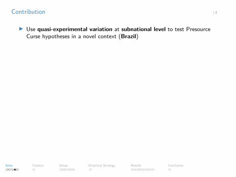
Contribution | 4
I Use quasi-experimental variation at subnational level to test PresourceCurse hypotheses in a novel context (Brazil)
I Harness municipality panel data to explore dynamic governance outcomes(public finances, public goods provision, electoral competition, patronage)
Methodological contribution: quantify heterogeneity in discovery realizations
I “Satisfied” places–where discoveries are realized–are those typically studied inthe resource curse literature → Do satisfied places anticipate booms orexhibit long-run resource curse symptoms?
I “Disappointed” places–treated by discoveries that never produce–are oftenlumped in with controls (e.g., no resource revenues) or satisfied places (e.g.,treated by discovery) → Do disappointed places experience negativeoutcomes after discoveries?
Intro Context Setup Empirical Strategy Results Conclusion
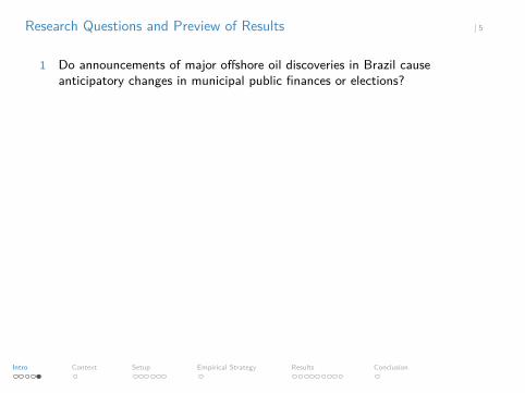
Research Questions and Preview of Results | 5
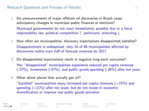
1 Do announcements of major offshore oil discoveries in Brazil causeanticipatory changes in municipal public finances or elections?
Municipal governments do not react immediately, possibly due to a fiscalresponsibility law; political competition ↑, politicians’ schooling ↓
2 How often are municipalities’ discovery expectations disappointed/satisfied?Disappointment is widespread: only 18 of 48 municipalities affected bydiscoveries realize even half of forecast revenues by 2017
3 Do disappointed expectations result in negative long-term outcomes?Yes, “disappointed” municipalities experience reduced per capita revenues(-27%), investment (-57%), and public goods spending (-26%) after ten years
4 What about places that actually get oil?“Satisfied” municipalities enjoy increased per capita revenues (+75%) andspending (+21%) after ten years, but do not invest in economicdiversification or improve real public goods provision
Intro Context Setup Empirical Strategy Results Conclusion

Research Questions and Preview of Results | 5
1 Do announcements of major offshore oil discoveries in Brazil causeanticipatory changes in municipal public finances or elections?Municipal governments do not react immediately, possibly due to a fiscalresponsibility law; political competition ↑, politicians’ schooling ↓
2 How often are municipalities’ discovery expectations disappointed/satisfied?
Disappointment is widespread: only 18 of 48 municipalities affected bydiscoveries realize even half of forecast revenues by 2017
3 Do disappointed expectations result in negative long-term outcomes?Yes, “disappointed” municipalities experience reduced per capita revenues(-27%), investment (-57%), and public goods spending (-26%) after ten years
4 What about places that actually get oil?“Satisfied” municipalities enjoy increased per capita revenues (+75%) andspending (+21%) after ten years, but do not invest in economicdiversification or improve real public goods provision
Intro Context Setup Empirical Strategy Results Conclusion
Research Questions and Preview of Results | 5
1 Do announcements of major offshore oil discoveries in Brazil causeanticipatory changes in municipal public finances or elections?Municipal governments do not react immediately, possibly due to a fiscalresponsibility law; political competition ↑, politicians’ schooling ↓
2 How often are municipalities’ discovery expectations disappointed/satisfied?Disappointment is widespread: only 18 of 48 municipalities affected bydiscoveries realize even half of forecast revenues by 2017
3 Do disappointed expectations result in negative long-term outcomes?Yes, “disappointed” municipalities experience reduced per capita revenues(-27%), investment (-57%), and public goods spending (-26%) after ten years
4 What about places that actually get oil?“Satisfied” municipalities enjoy increased per capita revenues (+75%) andspending (+21%) after ten years, but do not invest in economicdiversification or improve real public goods provision
Intro Context Setup Empirical Strategy Results Conclusion
Research Questions and Preview of Results | 5
1 Do announcements of major offshore oil discoveries in Brazil causeanticipatory changes in municipal public finances or elections?Municipal governments do not react immediately, possibly due to a fiscalresponsibility law; political competition ↑, politicians’ schooling ↓
2 How often are municipalities’ discovery expectations disappointed/satisfied?Disappointment is widespread: only 18 of 48 municipalities affected bydiscoveries realize even half of forecast revenues by 2017
3 Do disappointed expectations result in negative long-term outcomes?
Yes, “disappointed” municipalities experience reduced per capita revenues(-27%), investment (-57%), and public goods spending (-26%) after ten years
4 What about places that actually get oil?“Satisfied” municipalities enjoy increased per capita revenues (+75%) andspending (+21%) after ten years, but do not invest in economicdiversification or improve real public goods provision
Intro Context Setup Empirical Strategy Results Conclusion
Research Questions and Preview of Results | 5
1 Do announcements of major offshore oil discoveries in Brazil causeanticipatory changes in municipal public finances or elections?Municipal governments do not react immediately, possibly due to a fiscalresponsibility law; political competition ↑, politicians’ schooling ↓
2 How often are municipalities’ discovery expectations disappointed/satisfied?Disappointment is widespread: only 18 of 48 municipalities affected bydiscoveries realize even half of forecast revenues by 2017
3 Do disappointed expectations result in negative long-term outcomes?Yes, “disappointed” municipalities experience reduced per capita revenues(-27%), investment (-57%), and public goods spending (-26%) after ten years
4 What about places that actually get oil?“Satisfied” municipalities enjoy increased per capita revenues (+75%) andspending (+21%) after ten years, but do not invest in economicdiversification or improve real public goods provision
Intro Context Setup Empirical Strategy Results Conclusion
Research Questions and Preview of Results | 5
1 Do announcements of major offshore oil discoveries in Brazil causeanticipatory changes in municipal public finances or elections?Municipal governments do not react immediately, possibly due to a fiscalresponsibility law; political competition ↑, politicians’ schooling ↓
2 How often are municipalities’ discovery expectations disappointed/satisfied?Disappointment is widespread: only 18 of 48 municipalities affected bydiscoveries realize even half of forecast revenues by 2017
3 Do disappointed expectations result in negative long-term outcomes?Yes, “disappointed” municipalities experience reduced per capita revenues(-27%), investment (-57%), and public goods spending (-26%) after ten years
4 What about places that actually get oil?
“Satisfied” municipalities enjoy increased per capita revenues (+75%) andspending (+21%) after ten years, but do not invest in economicdiversification or improve real public goods provision
Intro Context Setup Empirical Strategy Results Conclusion
Research Questions and Preview of Results | 5
1 Do announcements of major offshore oil discoveries in Brazil causeanticipatory changes in municipal public finances or elections?Municipal governments do not react immediately, possibly due to a fiscalresponsibility law; political competition ↑, politicians’ schooling ↓
2 How often are municipalities’ discovery expectations disappointed/satisfied?Disappointment is widespread: only 18 of 48 municipalities affected bydiscoveries realize even half of forecast revenues by 2017
3 Do disappointed expectations result in negative long-term outcomes?Yes, “disappointed” municipalities experience reduced per capita revenues(-27%), investment (-57%), and public goods spending (-26%) after ten years
4 What about places that actually get oil?“Satisfied” municipalities enjoy increased per capita revenues (+75%) andspending (+21%) after ten years, but do not invest in economicdiversification or improve real public goods provision
Intro Context Setup Empirical Strategy Results Conclusion
Brazil’s Pre-Salt Discoveries: A Winning Lottery Ticket? | 6
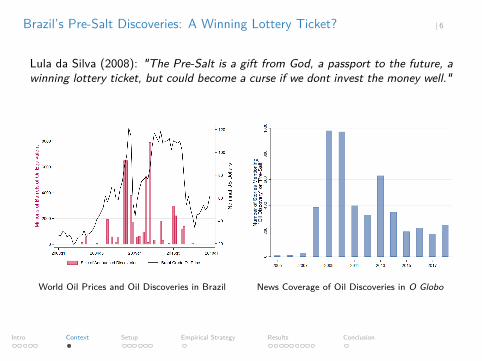
Lula da Silva (2008): "The Pre-Salt is a gift from God, a passport to the future, awinning lottery ticket, but could become a curse if we dont invest the money well."
World Oil Prices and Oil Discoveries in Brazil News Coverage of Oil Discoveries in O Globo
Intro Context Setup Empirical Strategy Results Conclusion

Exploiting a Quasi-Experiment I: Discovery Announcements | 7
I compile a comprehensive geolocated dataset of 179 offshore discoveryannouncements filed by oil companies with Brazil’s SEC (CVM) from 2000-2017
"Communication to the Market" Filed by Petrobras with Comissão deValores Mobiliários
Intro Context Setup Empirical Strategy Results Conclusion
Exploiting a Quasi-Experiment II: Royalty Distribution Maps | 8
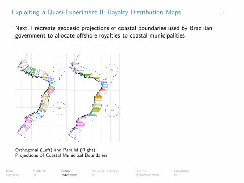
Next, I recreate geodesic projections of coastal boundaries used by Braziliangovernment to allocate offshore royalties to coastal municipalities
Orthogonal (Left) and Parallel (Right)Projections of Coastal Municipal Boundaries
Offshore Wells Overlaid on OrthogonalProjections (Example: Rio de Janeiro)
Intro Context Setup Empirical Strategy Results Conclusion

Exploiting a Quasi-Experiment II: Royalty Distribution Maps | 8
Next, I recreate geodesic projections of coastal boundaries used by Braziliangovernment to allocate offshore royalties to coastal municipalities
Orthogonal (Left) and Parallel (Right)Projections of Coastal Municipal Boundaries
Offshore Wells Overlaid on OrthogonalProjections (Example: Rio de Janeiro)
Intro Context Setup Empirical Strategy Results Conclusion

Exploiting a Quasi-Experiment III: Forecasting Revenue Expectations | 9
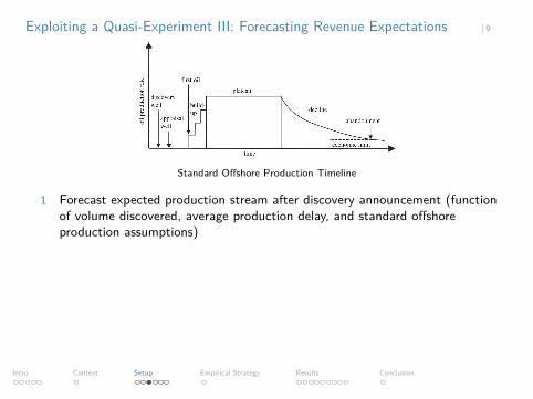
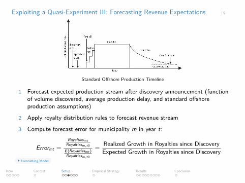
Standard Offshore Production Timeline
1 Forecast expected production stream after discovery announcement (functionof volume discovered, average production delay, and standard offshoreproduction assumptions)
2 Apply royalty distribution rules to forecast revenue stream
3 Compute forecast error for municipality m in year t:
Errormt =Royaltiesmt
Royaltiesm,t0E(Royaltiesmt )Royaltiesm,t0
= Realized Growth in Royalties since DiscoveryExpected Growth in Royalties since Discovery
Forecasting Model
Intro Context Setup Empirical Strategy Results Conclusion
Exploiting a Quasi-Experiment III: Forecasting Revenue Expectations | 9
Standard Offshore Production Timeline
1 Forecast expected production stream after discovery announcement (functionof volume discovered, average production delay, and standard offshoreproduction assumptions)
2 Apply royalty distribution rules to forecast revenue stream
3 Compute forecast error for municipality m in year t:
Errormt =Royaltiesmt
Royaltiesm,t0E(Royaltiesmt )Royaltiesm,t0
= Realized Growth in Royalties since DiscoveryExpected Growth in Royalties since Discovery
Forecasting Model
Intro Context Setup Empirical Strategy Results Conclusion
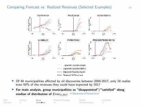
Comparing Forecast vs. Realized Revenues (Selected Examples) | 10
I Of 48 municipalities affected by oil discoveries between 2000-2017, only 18 realizeeven 50% of the revenues they could have expected by 2017
I For main analysis, group municipalities as "disappointed"/"satisfied" alongmedian of distribution of Errorm,2017 Distributions of Forecast Error
Intro Context Setup Empirical Strategy Results Conclusion
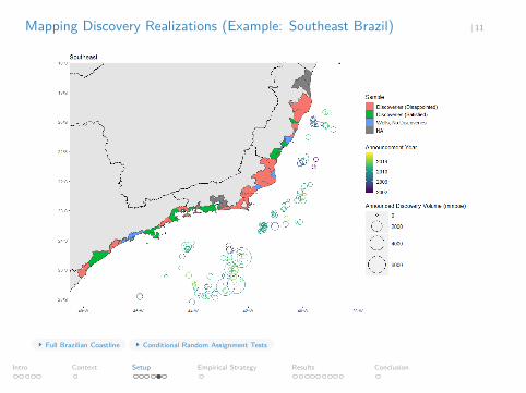
Mapping Discovery Realizations (Example: Southeast Brazil) | 11
Full Brazilian Coastline Conditional Random Assignment Tests
Intro Context Setup Empirical Strategy Results Conclusion

Data Sources: Constructing a Rich Municipality-Level Panel | 12
Data Source YearsDiscovery Announcements CVM 2002-2017Oil Royalties & Special Participations ANP 1999-2017Offshore Well Shapefiles ANP 2000-2017Oil and Gas Production ANP 2005-2017
Public Finances FINBRA & IPEA 2000-2017Employment & Firm Entry RAIS 2000-2017Federal and State Transfers Tesouro Nacional 2000-2017Elections (Candidates and Donors) TSE 2000-2016
Health Indicators SUS 2000-2017Education Indicators Basic Ed Census 2000-2017Education Outcomes IDEB 2005-2017
Municipal Development Index FIRJAN 2000, 2005-2016Municipality Characteristics Census 2000, 2010
Brent Crude Oil Prices FRED 2000-2017Currency Deflator IPEA (INPC) 2000-2017Interest Rate IPEA (Selic) 2000-2017
Balance Across Samples
Intro Context Setup Empirical Strategy Results Conclusion

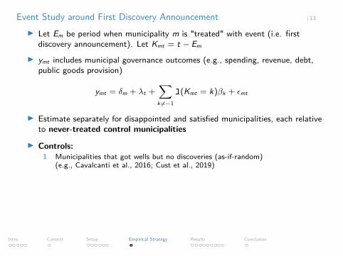
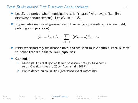
Event Study around First Discovery Announcement | 13
I Let Em be period when municipality m is "treated" with event (i.e. firstdiscovery announcement). Let Kmt = t − Em
I ymt includes municipal governance outcomes (e.g., spending, revenue, debt,public goods provision)
ymt = δm + λt +∑k 6=−1
1(Kmt = k)βk + εmt
I Estimate separately for disappointed and satisfied municipalities, each relativeto never-treated control municipalities
I Controls:1 Municipalities that got wells but no discoveries (as-if-random)
(e.g., Cavalcanti et al., 2016; Cust et al., 2019)2 Pre-matched municipalities (coarsened exact matching)
I Estimators:1 Two-way fixed effects (TWFE)2 Callaway and Sant’Anna (2020) staggered event study estimator (CS)
Identification
Intro Context Setup Empirical Strategy Results Conclusion
Event Study around First Discovery Announcement | 13
I Let Em be period when municipality m is "treated" with event (i.e. firstdiscovery announcement). Let Kmt = t − Em
I ymt includes municipal governance outcomes (e.g., spending, revenue, debt,public goods provision)
ymt = δm + λt +∑k 6=−1
1(Kmt = k)βk + εmt
I Estimate separately for disappointed and satisfied municipalities, each relativeto never-treated control municipalities
I Controls:1 Municipalities that got wells but no discoveries (as-if-random)
(e.g., Cavalcanti et al., 2016; Cust et al., 2019)
2 Pre-matched municipalities (coarsened exact matching)
I Estimators:1 Two-way fixed effects (TWFE)2 Callaway and Sant’Anna (2020) staggered event study estimator (CS)
Identification
Intro Context Setup Empirical Strategy Results Conclusion
Event Study around First Discovery Announcement | 13
I Let Em be period when municipality m is "treated" with event (i.e. firstdiscovery announcement). Let Kmt = t − Em
I ymt includes municipal governance outcomes (e.g., spending, revenue, debt,public goods provision)
ymt = δm + λt +∑k 6=−1
1(Kmt = k)βk + εmt
I Estimate separately for disappointed and satisfied municipalities, each relativeto never-treated control municipalities
I Controls:1 Municipalities that got wells but no discoveries (as-if-random)
(e.g., Cavalcanti et al., 2016; Cust et al., 2019)2 Pre-matched municipalities (coarsened exact matching)
I Estimators:1 Two-way fixed effects (TWFE)2 Callaway and Sant’Anna (2020) staggered event study estimator (CS)
Identification
Intro Context Setup Empirical Strategy Results Conclusion
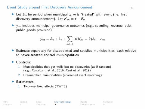
Event Study around First Discovery Announcement | 13
I Let Em be period when municipality m is "treated" with event (i.e. firstdiscovery announcement). Let Kmt = t − Em
I ymt includes municipal governance outcomes (e.g., spending, revenue, debt,public goods provision)
ymt = δm + λt +∑k 6=−1
1(Kmt = k)βk + εmt
I Estimate separately for disappointed and satisfied municipalities, each relativeto never-treated control municipalities
I Controls:1 Municipalities that got wells but no discoveries (as-if-random)
(e.g., Cavalcanti et al., 2016; Cust et al., 2019)2 Pre-matched municipalities (coarsened exact matching)
I Estimators:1 Two-way fixed effects (TWFE)
2 Callaway and Sant’Anna (2020) staggered event study estimator (CS)Identification
Intro Context Setup Empirical Strategy Results Conclusion
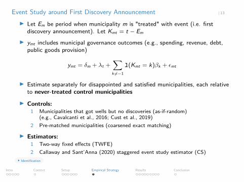
Event Study around First Discovery Announcement | 13
I Let Em be period when municipality m is "treated" with event (i.e. firstdiscovery announcement). Let Kmt = t − Em
I ymt includes municipal governance outcomes (e.g., spending, revenue, debt,public goods provision)
ymt = δm + λt +∑k 6=−1
1(Kmt = k)βk + εmt
I Estimate separately for disappointed and satisfied municipalities, each relativeto never-treated control municipalities
I Controls:1 Municipalities that got wells but no discoveries (as-if-random)
(e.g., Cavalcanti et al., 2016; Cust et al., 2019)2 Pre-matched municipalities (coarsened exact matching)
I Estimators:1 Two-way fixed effects (TWFE)2 Callaway and Sant’Anna (2020) staggered event study estimator (CS)
Identification
Intro Context Setup Empirical Strategy Results Conclusion
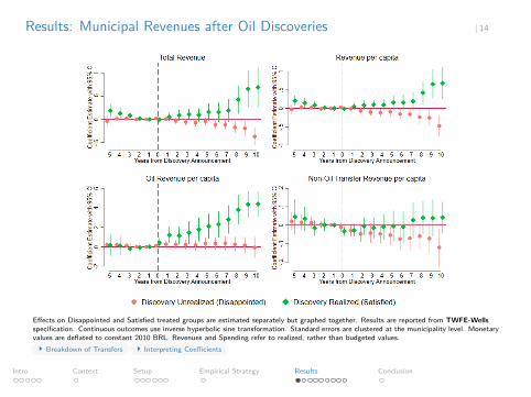
Results: Municipal Revenues after Oil Discoveries | 14
Effects on Disappointed and Satisfied treated groups are estimated separately but graphed together. Results are reported from TWFE-Wellsspecification. Continuous outcomes use inverse hyperbolic sine transformation. Standard errors are clustered at the municipality level. Monetaryvalues are deflated to constant 2010 BRL. Revenues and Spending refer to realized, rather than budgeted values.
Breakdown of Transfers Interpreting Coefficients
Intro Context Setup Empirical Strategy Results Conclusion
+5441%
+75%
−27%
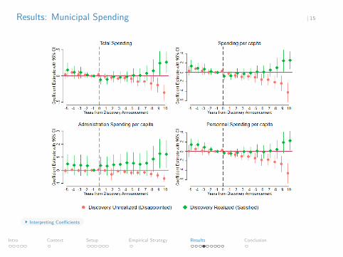
Results: Municipal Spending | 15
Interpreting Coefficients
Intro Context Setup Empirical Strategy Results Conclusion
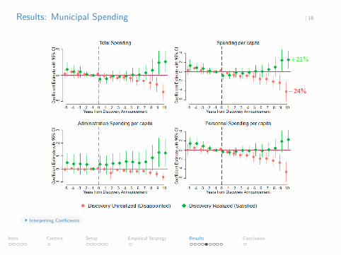
Results: Municipal Spending | 16
Interpreting Coefficients
Intro Context Setup Empirical Strategy Results Conclusion
+21%
−24%

Results: Investment and Economic Diversification | 17
Interpreting Coefficients
Intro Context Setup Empirical Strategy Results Conclusion
−57%
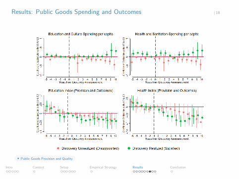
Results: Public Goods Spending and Outcomes | 18
Public Goods Provision and Quality
Intro Context Setup Empirical Strategy Results Conclusion
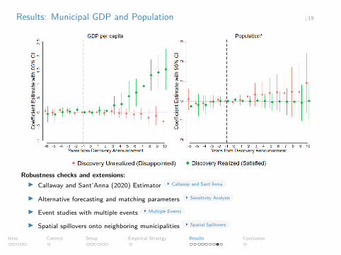
Results: Municipal GDP and Population | 19
Robustness checks and extensions:I Callaway and Sant’Anna (2020) Estimator Callaway and Sant’Anna
I Alternative forecasting and matching parameters Sensitivity Analysis
I Event studies with multiple events Multiple Events
I Spatial spillovers onto neighboring municipalities Spatial Spillovers
Intro Context Setup Empirical Strategy Results Conclusion
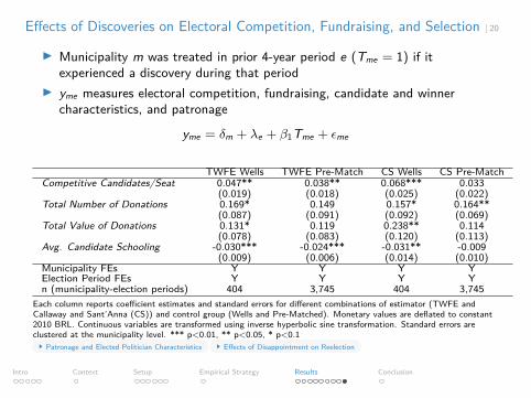
Effects of Discoveries on Electoral Competition, Fundraising, and Selection | 20
I Municipality m was treated in prior 4-year period e (Tme = 1) if itexperienced a discovery during that period
I yme measures electoral competition, fundraising, candidate and winnercharacteristics, and patronage
yme = δm + λe + β1Tme + εme
TWFE Wells TWFE Pre-Match CS Wells CS Pre-MatchCompetitive Candidates/Seat 0.047** 0.038** 0.068*** 0.033
(0.019) (0.018) (0.025) (0.022)Total Number of Donations 0.169* 0.149 0.157* 0.164**
(0.087) (0.091) (0.092) (0.069)Total Value of Donations 0.131* 0.119 0.238** 0.114
(0.078) (0.083) (0.120) (0.113)Avg. Candidate Schooling -0.030*** -0.024*** -0.031** -0.009
(0.009) (0.006) (0.014) (0.010)Municipality FEs Y Y Y YElection Period FEs Y Y Y Yn (municipality-election periods) 404 3,745 404 3,745
Each column reports coefficient estimates and standard errors for different combinations of estimator (TWFE andCallaway and Sant’Anna (CS)) and control group (Wells and Pre-Matched). Monetary values are deflated to constant2010 BRL. Continuous variables are transformed using inverse hyperbolic sine transformation. Standard errors areclustered at the municipality level. *** p<0.01, ** p<0.05, * p<0.1
Patronage and Elected Politician Characteristics Effects of Disappointment on Reelection
Intro Context Setup Empirical Strategy Results Conclusion
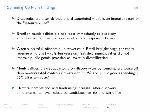
Summing Up Main Findings | 21
I Discoveries are often delayed and disappointed – this is an important part ofthe "resource curse"
I Brazilian municipalities did not react immediately to discoveryannouncements, possibly because of a fiscal responsibility law
I When successful, offshore oil discoveries in Brazil brought huge per capitarevenue windfalls (+75% ten years on); satisfied municipalities did notimprove public goods provision or invest in diversification
I Municipalities left disappointed after discovery announcements are worse offthan never-treated controls (investment ↓ 57% and public goods spending ↓26% after ten years)
I Electoral competition and fundraising increases after discoveryannouncements; lower educated candidates run for and win office
Intro Context Setup Empirical Strategy Results Conclusion

Forecasting Municipalities’ Discovery Expectations I | 22
Standard Offshore Production Timeline
Municipality m’s expected production stream from discovery d in year t:
E(Productionmdt ) =
{1(alignmentmd = 1) × δVd × (t−t0)
θstif t − t0 ≤ θst
1(alignmentmd = 1) × δVd if t − t0 > θst
I t0 is year of discovery announcementI Vd is volume of the announced discoveryI δ is proportion of total reserve extracted each year (US EIA, 2015)I θst is average discovery-to-production delay in sedimentary basin s up to year t
Appendices
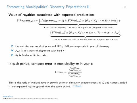
Forecasting Municipalities’ Discovery Expectations II | 23
Value of royalties associated with expected production:E(Royaltiesmdt ) =
(1(alignmentmw = 1) × E(Prodmdt ) × (Pt0 × Xt0) × 0.30 × 0.05
)︸ ︷︷ ︸First 5% of Royalty Tax to Municipalities Aligned with Well
+
(E(Prodmdt ) × (Pt0 × Xt0) × 0.225 × (Rf − 0.05) × Amf
)︸ ︷︷ ︸Tax in Excess of 5% to Municipalities Aligned with Field
I Pt0 and Xt0 are world oil price and BRL/USD exchange rate in year of discoveryI Amf is m’s share of alignment with field fI Rf is field-specific tax rate
In each period, compute error in municipality m in year t:
Errormt =Royaltiesmt
Royaltiesm,t0E(Royaltiesmt )Royaltiesm,t0
This is the ratio of realized royalty growth between discovery announcement in t0 and current periodt, and expected royalty growth over the same period. Return
Appendices
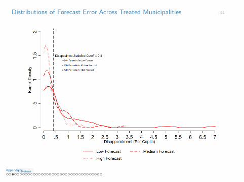
Distributions of Forecast Error Across Treated Municipalities | 24
ReturnAppendices

Pre-Treatment (Year 2000) Balance Between Samples | 25
Treated Samples Control SamplesDisappoint. Satisfied Wells Match (D) Match (S) Coastal
Latitude -19.50 -21.82 -13.04 -20.21 -20.00 -16.40(6.25) (3.13) (9.59) (7.91) (8.13) (9.24)
Dist. from State Capital 116.62 88.59 150.15 192.14 92.79 248.87(85.35) (57.12) (120.02) (143.64) (38.81) (159.90)
Population (Thousands) 91.88 398.53 55.42 38.11 56.82 32.26(122.23) (1,367.51) (81.82) (77.30) (471.41) (192.54)
GDP per capita 17,769 13,779 6,552 6,814 7,840 5,443(26,418) (12,003) (6,735) (7,261) (9,641) (5,978)
Income Gini Coefficient 0.57 0.57 0.56 0.55 0.53 0.54(0.05) (0.04) (0.07) (0.06) (0.06) (0.07)
Municipal Dev.Index 0.60 0.64 0.50 0.57 0.57 0.53(0.07) (0.09) (0.10) (0.09) (0.13) (0.13)
Urban Share of Pop. 0.83 0.80 0.66 0.68 0.66 0.57(0.21) (0.22) (0.24) (0.20) (0.25) (0.24)
% HHs w. Water/Sewer 7.76 3.63 20.56 10.03 10.67 13.64(8.01) (3.95) (19.57) (12.19) (15.81) (16.19)
Municipal Revenue p.c. 1,628 1,729 1,011 969 1,220 1,000(1,478) (1,047) (809) (2,993) (3,840) (1,496)
Municipal Oil Rev. p.c. 420.6 161.8 129.7 15.1 10.2 6.1(999.4) (334.7) (412.9) (100.4) (43.4) (60.0)
Municipal Invest. p.c. 161.0 123.1 98.2 55.0 69.7 63.3(223.9) (110.3) (172.1) (116.9) (143.8) (83.2)
n 30 18 53 836 500 3,902
Sample means with standard deviations in parentheses. Monetary values are deflated to constant 2010 Brazilian Reals. Return
Appendices
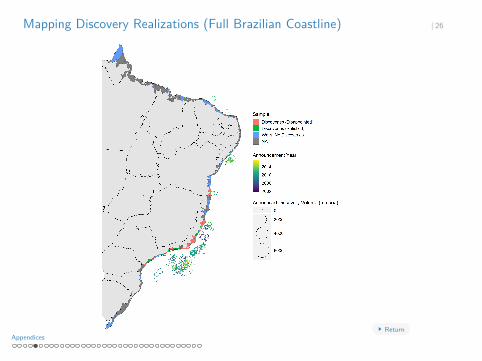
Mapping Discovery Realizations (Full Brazilian Coastline) | 26
ReturnAppendices

Testing Conditional Random Assignment | 27
Regress characteristic Ym from baseline year 2000 on a vector of geographiccontrols, state FEs, and a treatment indicator that equals 1 if:
1 Municipality has wells drilled
2 A major discovery is announced in municipalities where wells were drilled
3 Expectations are satisfied in municipalities that received discoveryannouncements
Y 2000m = α + β1Treatmentm + X ′
mλ + δs + εm
Appendices
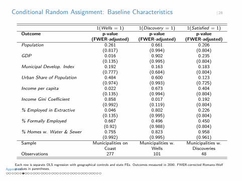
Conditional Random Assignment: Baseline Characteristics | 28
1(Wells = 1) 1(Discovery = 1) 1(Satisfied = 1)Outcome p-value p-value p-value
(FWER-adjusted) (FWER-adjusted) (FWER-adjusted)Population 0.261 0.661 0.206
(0.817) (0.994) (0.804)GDP 0.016 0.902 0.235
(0.135) (0.995) (0.804)Municipal Develop. Index 0.192 0.163 0.183
(0.777) (0.684) (0.804)Urban Share of Population 0.484 0.600 0.123
(0.974) (0.993) (0.725)Income per capita 0.022 0.673 0.404
(0.135) (0.994) (0.804)Income Gini Coefficient 0.858 0.017 0.192
(0.992) (0.119) (0.804)% Employed in Extractive 0.046 0.802 0.226
(0.135) (0.995) (0.804)% Formally Employed 0.667 0.496 0.450
(0.92) (0.988) (0.804)% Homes w. Water & Sewer 0.755 0.823 0.958
(0.992) (0.995) (0.961)Sample Municipalities on Municipalities w. Municipalities w.
Coast Wells DiscoveriesObservations 277 101 48
Each row is separate OLS regression with geographical controls and state FEs. Outcomes measured in 2000. FWER-corrected Romano-Wolfp-values in parentheses.Appendices

Conditional Random Assigment: Political Alignment | 29
1(Wells = 1) 1(Discovery = 1) 1(Satisfied = 1)Outcome p-value p-value p-value
(FWER-adj.) (FWER-adj.) (FWER-adj.)Cumulative Party Align. w. Governor 0.417 0.604 0.926
(0.668) (0.879) (0.937)Cumulative Party Align. w. President 0.953 0.680 0.160
(0.963) (0.879) (0.521)State Capital Dummy 0.091 0.745 0.198
(0.283) (0.879) (0.521)Contemp. Party Align. w. Governor 0.745 0.387 NA
Contemp. Party Align. w. President 0.558 0.550 NA
State Capital Dummy 0.000 0.973 NA
Sample Municipalities on Municipalities w. Municipalities w.Coast Wells Discoveries
Observations 277 101 48
I Cumulative party alignment measures number of years between 2000-2017 in which municipalmayor was of same party as governor/president.
I Contemporaneous party alignment is indicator equal to 1 in years where municipal mayor’s partyis the same as governor/president’s party.
I Each row is separate OLS regression with geographical controls and state FEs. FWER-correctedRomano-Wolf p-values in parentheses. Return
Appendices
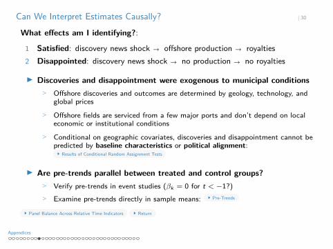
Can We Interpret Estimates Causally? | 30
What effects am I identifying?:
1 Satisfied: discovery news shock → offshore production → royalties2 Disappointed: discovery news shock → no production → no royalties
I Discoveries and disappointment were exogenous to municipal conditions> Offshore discoveries and outcomes are determined by geology, technology, and
global prices> Offshore fields are serviced from a few major ports and don’t depend on local
economic or institutional conditions> Conditional on geographic covariates, discoveries and disappointment cannot be
predicted by baseline characteristics or political alignment:Results of Conditional Random Assignment Tests
I Are pre-trends parallel between treated and control groups?> Verify pre-trends in event studies (βk = 0 for t < −1?)> Examine pre-trends directly in sample means: Pre-Trends
Panel Balance Across Relative Time Indicators Return
Appendices
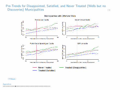
Pre-Trends for Disappointed, Satisfied, and Never Treated (Wells but noDiscoveries) Municipalities | 31
Return
Appendices

Pre-Trends for Disappointed, Satisfied, and Never Treated (Pre-Matched)Municipalities | 32
Return
Appendices

Sample Means Across Unbalanced Panel | 33
Return
Appendices
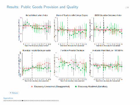
Results: Public Goods Provision and Quality | 34
Return
Appendices
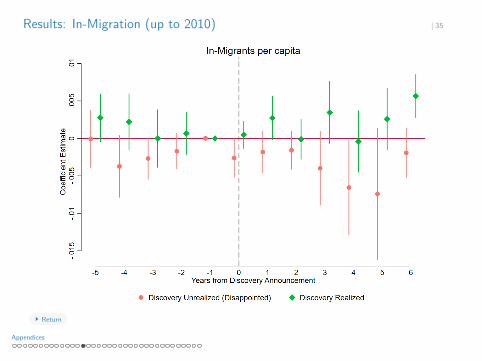
Results: In-Migration (up to 2010) | 35
Return
Appendices
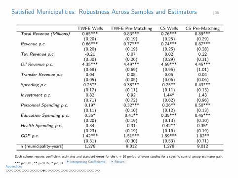
Satisfied Municipalities: Robustness Across Samples and Estimators | 36
TWFE Wells TWFE Pre-Matching CS Wells CS Pre-MatchingTotal Revenue (Millions) 0.65*** 0.83*** 0.76*** 0.89***
(0.20) (0.19) (0.25) (0.29)Revenue p.c. 0.66*** 0.77*** 0.74*** 0.87***
(0.20) (0.19) (0.25) (0.28)Tax Revenue p.c. -0.21 0.07 0.02 0.22
(0.30) (0.26) (0.29) (0.31)Oil Revenue p.c. 4.35*** 4.49*** 4.69*** 4.45***
(0.68) (0.69) (0.95) (1.01)Transfer Revenue p.c. 0.04 0.08 0.05 0.04
(0.05) (0.05) (0.06) (0.06)Spending p.c. 0.25** 0.38*** 0.25** 0.43***
(0.12) (0.11) (0.11) (0.13)Investment p.c. 0.82 0.92 1.44* 1.43
(0.71) (0.72) (0.82) (0.96)Personnel Spending p.c. 0.19* 0.32*** 0.26** 0.50***
(0.11) (0.10) (0.12) (0.13)Education Spending p.c. 0.35* 0.41** 0.35*** 0.45***
(0.20) (0.19) (0.13) (0.10)Health Spending p.c. 0.34 0.31 0.42** 0.35*
(0.23) (0.19) (0.19) (0.19)GDP p.c. 1.42*** 1.51*** 1.59*** 1.82**
(0.31) (0.30) (0.53) (0.71)n (municipality-years) 1,278 9,012 1,278 9,012
Each column reports coefficient estimates and standard errors for the t + 10 period of event studies for a specific control group-estimator pair.
*** p<0.01, ** p<0.05, * p<0.1 Interpreting Coefficients ReturnAppendices
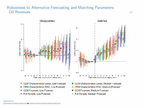
Robustness to Alternative Forecasting and Matching Parameters:Oil Revenues | 37
Appendices
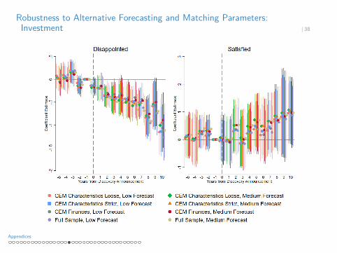
Robustness to Alternative Forecasting and Matching Parameters:Investment | 38
Appendices

Robustness to Alternative Forecasting and Matching Parameters:Education Spending | 39
Appendices

Robustness to Alternative Forecasting and Matching Parameters:GDP | 40
ReturnAppendices
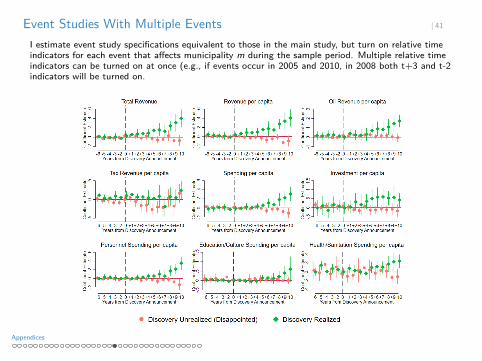
Event Studies With Multiple Events | 41
I estimate event study specifications equivalent to those in the main study, but turn on relative timeindicators for each event that affects municipality m during the sample period. Multiple relative timeindicators can be turned on at once (e.g., if events occur in 2005 and 2010, in 2008 both t+3 and t-2indicators will be turned on.
Appendices
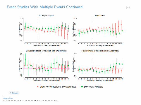
Event Studies With Multiple Events Continued | 42
Return
Appendices
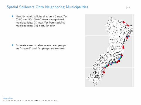
Spatial Spillovers Onto Neighboring Municipalities | 43
I Identify municipalities that are (i) near/far(0-50 and 50-100km) from disappointedmunicipalities; (ii) near/far from satisfiedmunicipalities; (iii) near/far both
I Estimate event studies where near groupsare "treated" and far groups are controls
Appendices
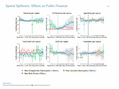
Spatial Spillovers: Effects on Public Finances | 44
Appendices

Spatial Spillovers: Effects on Firm Entry | 45
ReturnAppendices

Discovery Effects on Formal Employment | 46
Appendices

Discovery Effects on Firm Entry | 47
Return
Appendices
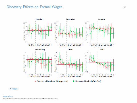
Discovery Effects on Formal Wages | 48
Return
Appendices
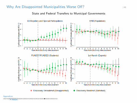
Why Are Disappointed Municipalities Worse Off? | 49
State and Federal Transfers to Municipal Governments
ReturnAppendices

Do Voters Punish Incumbents for Discovery Disappointment? | 50
Estimate likelihood of reelection for incumbent i in municipality m and election period e:P(Reelectionime = 1) = δm + λe + βDisappointedme + X ′
i µ + εime
Appendices
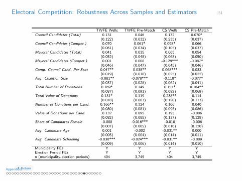
Electoral Competition: Robustness Across Samples and Estimators | 51
TWFE Wells TWFE Pre-Match CS Wells CS Pre-MatchCouncil Candidates (Total) 0.131 0.046 0.172 0.070*
(0.122) (0.032) (0.235) (0.037)Council Candidates (Compet.) 0.070 0.061* 0.098* 0.066
(0.061) (0.034) (0.105) (0.037)Mayoral Candidates (Total) 0.041 0.035 0.065 0.054
(0.052) (0.048) (0.068) (0.050)Mayoral Candidates (Compet.) 0.001 0.008 -0.129*** -0.087*
(0.046) (0.047) (0.045) (0.046)Comp. Council Cand. Per Seat 0.047** 0.038** 0.068*** 0.033
(0.019) (0.018) (0.025) (0.022)Avg. Coalition Size -0.081** -0.078*** -0.118* -0.077*
(0.037) (0.028) (0.062) (0.041)Total Number of Donations 0.169* 0.149 0.157* 0.164**
(0.087) (0.091) (0.092) (0.069)Total Value of Donations 0.131* 0.119 0.238** 0.114
(0.078) (0.083) (0.120) (0.113)Number of Donations per Cand. 0.166** 0.124 0.106 0.040
(0.080) (0.081) (0.095) (0.086)Value of Donations per Cand. 0.132 0.095 0.195 -0.006
(0.082) (0.085) (0.137) (0.128)Share of Candidates Female -0.008 -0.016*** -0.010 -0.006
(0.007) (0.005) (0.010) (0.120)Avg. Candidate Age 0.001 -0.002 -0.031** 0.000
(0.005) (0.004) (0.014) (0.011)Avg. Candidate Schooling -0.030*** -0.024*** -0.031** -0.009
(0.009) (0.006) (0.014) (0.010)Municipality FEs Y Y Y YElection Period FEs Y Y Y Yn (municipality-election periods) 404 3,745 404 3,745
ReturnAppendices
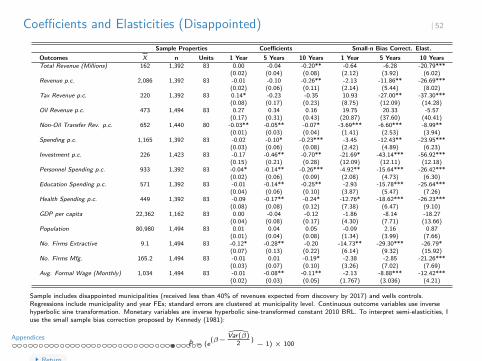
Coefficients and Elasticities (Disappointed) | 52
Sample Properties Coefficients Small-n Bias Correct. Elast.Outcomes X n Units 1 Year 5 Years 10 Years 1 Year 5 Years 10 YearsTotal Revenue (Millions) 162 1,392 83 0.00 -0.04 -0.20** -0.64 -6.28 -20.79***
(0.02) (0.04) (0.08) (2.12) (3.92) (6.02)Revenue p.c. 2,086 1,392 83 -0.01 -0.10 -0.26** -2.13 -11.86** -26.69***
(0.02) (0.06) (0.11) (2.14) (5.44) (8.02)Tax Revenue p.c. 220 1,392 83 0.14* -0.23 -0.35 10.93 -27.00** -37.30***
(0.08) (0.17) (0.23) (8.75) (12.09) (14.28)Oil Revenue p.c. 473 1,494 83 0.27 0.34 0.16 19.75 20.33 -5.57
(0.17) (0.31) (0.43) (20.87) (37.60) (40.41)Non-Oil Transfer Rev. p.c. 652 1,440 80 -0.03** -0.05** -0.07* -3.69*** -6.60*** -8.99**
(0.01) (0.03) (0.04) (1.41) (2.53) (3.94)Spending p.c. 1,165 1,392 83 -0.02 -0.10* -0.23*** -3.45 -12.43** -23.95***
(0.03) (0.06) (0.08) (2.42) (4.89) (6.23)Investment p.c. 226 1,423 83 -0.17 -0.46** -0.70** -21.69* -43.14*** -56.92***
(0.15) (0.21) (0.28) (12.09) (12.11) (12.18)Personnel Spending p.c. 933 1,392 83 -0.04* -0.14** -0.26*** -4.92** -15.64*** -26.42***
(0.02) (0.06) (0.09) (2.08) (4.73) (6.30)Education Spending p.c. 571 1,392 83 -0.01 -0.14** -0.25** -2.93 -15.78*** -25.64***
(0.04) (0.06) (0.10) (3.87) (5.47) (7.26)Health Spending p.c. 449 1,392 83 -0.09 -0.17** -0.24* -12.76* -18.62*** -26.23***
(0.08) (0.08) (0.12) (7.38) (6.47) (9.10)GDP per capita 22,362 1,162 83 0.00 -0.04 -0.12 -1.86 -8.14 -18.27
(0.04) (0.08) (0.17) (4.30) (7.71) (13.66)Population 80,980 1,494 83 0.01 0.04 0.05 -0.09 2.16 0.87
(0.01) (0.04) (0.08) (1.34) (3.99) (7.66)No. Firms Extractive 9.1 1,494 83 -0.12* -0.28** -0.20 -14.73** -29.30*** -26.79*
(0.07) (0.13) (0.22) (6.14) (9.32) (15.92)No. Firms Mfg. 165.2 1,494 83 -0.01 0.01 -0.19* -2.38 -2.85 -21.26***
(0.03) (0.07) (0.10) (3.26) (7.02) (7.69)Avg. Formal Wage (Monthly) 1,034 1,494 83 -0.01 -0.08** -0.11** -2.13 -8.88*** -12.42***
(0.02) (0.03) (0.05) (1.767) (3.036) (4.21)
Sample includes disappointed municipalities (received less than 40% of revenues expected from discovery by 2017) and wells controls.Regressions include municipality and year FEs; standard errors are clustered at municipality level. Continuous outcome variables use inversehyperbolic sine transformation. Monetary variables are inverse hyperbolic sine-transformed constant 2010 BRL. To interpret semi-elasticities, Iuse the small sample bias correction proposed by Kennedy (1981):
P̂ = (e(β− V̂ar(β)2 ) − 1) × 100
Return
Appendices

Coefficients and Elasticities (Satisfied) | 53
Sample Properties Coefficients Small-n Bias Correct. Elast.Outcomes X n Units 1 Year 5 Years 10 Years 1 Year 5 Years 10 YearsTotal Revenue (Millions) 345 1,211 71 0.05 0.16* 0.65*** 3.01 11.74 74.53**
(0.04) (0.09) (0.20) (4.62) (10.43) (34.21)Revenue p.c. 2,361 1,211 71 0.05 0.16 0.66*** 2.74 11.69 75.12**
(0.04) (0.10) (0.20) (4.54) (10.91) (34.60)Tax Revenue p.c. 279 1,211 71 0.01 -0.06 -0.21 -3.23 -15.98 -30.32
(0.09) (0.23) (0.30) (8.68) (19.50) (20.58)Oil Revenue p.c. 606 1,278 71 1.21*** 2.10*** 4.35*** 170.90 490.53 5441.63
(0.42) (0.65) (0.68) (114.05) (383.00) (3755.01)Non-Oil Transfer Rev. p.c. 691 1,224 68 -0.03 -0.01 0.04 -3.63** -2.59 1.26
(0.02) (0.04) (0.05) (1.72) (4.10) (5.12)Spending p.c. 1,264 1,211 71 -0.07 0.01** 0.25** -9.00 -2.15 20.79
(0.05) (0.07) (0.12) (4.12) (6.55) (14.07)Investment p.c. 263 1,230 71 -0.06 0.34 0.82 -21.73 11.98 59.35
(0.37) (0.46) (0.71) (29.22) (51.91) (113.07)Personnel Spending p.c. 997 1,211 71 -0.04 0.01* 0.19* -5.86 -2.56 14.32
(0.03) (0.07) (0.11) (3.23) (6.87) (12.83)Education Spending p.c. 627 1,208 71 -0.01 0.03* 0.35 -4.62 0.07 28.02
(0.07) (0.07) (0.20) (6.40) (6.61) (26.10)Health Spending p.c. 461 1,208 71 0.20** 0.11 0.34 17.62* 6.88 25.42
(0.08) (0.09) (0.23) (9.90) (9.61) (29.05)GDP per capita 27,043 994 71 0.06 0.57** 1.42*** 2.56 55.00 253.10**
(0.08) (0.27) (0.31) (7.75) (42.12) (110.29)Population 155,964 1,278 71 0.00 -0.01 -0.01 -0.40 -1.63 -3.11
(0.01) (0.02) (0.05) (0.89) (2.17) (4.49)No. Firms Extractive 17.5 1,278 71 0.09 0.07 0.30 2.59 -1.89 18.90
(0.12) (0.17) (0.26) (12.29) (16.78) (31.23)No. Firms Mfg. 273.8 1,278 71 -0.09* -0.12** -0.23** -10.76** -13.70*** -25.03***
(0.05) (0.06) (0.11) (4.29) (4.76) (8.05)Avg. Formal Wage 1,073 1,278 71 -0.03 -0.01* -0.09** -4.17 -3.84 -11.06**
(0.02) (0.05) (0.05) (1.94) (4.72) (4.66)
Sample includes satisfied municipalities (received more than 40% of revenues expected from discovery by 2017) and wells controls. Regressionsinclude municipality and year FEs; standard errors are clustered at municipality level. Continuous outcome variables use inverse hyperbolic sinetransformation. Monetary variables are inverse hyperbolic sine-transformed constant 2010 BRL. To interpret semi-elasticities, I use the smallsample bias correction proposed by Kennedy (1981):
P̂ = (e(β− V̂ar(β)2 ) − 1) × 100
Return
Appendices
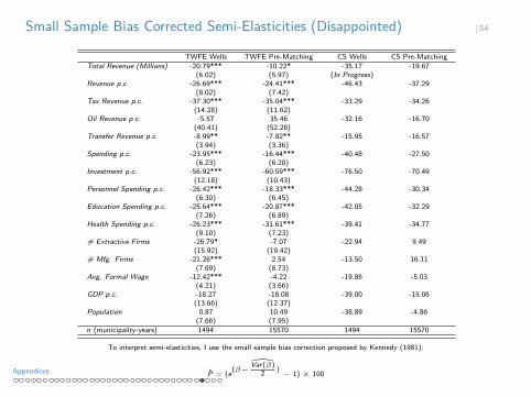
Small Sample Bias Corrected Semi-Elasticities (Disappointed) | 54
TWFE Wells TWFE Pre-Matching CS Wells CS Pre-MatchingTotal Revenue (Millions) -20.79*** -10.22* -35.17 -19.67
(6.02) (5.97) (In Progress)Revenue p.c. -26.69*** -24.41*** -46.43 -37.29
(8.02) (7.42)Tax Revenue p.c. -37.30*** -35.04*** -33.29 -34.26
(14.28) (11.62)Oil Revenue p.c. -5.57 35.46 -32.16 -16.70
(40.41) (52.28)Transfer Revenue p.c. -8.99** -7.82** -15.95 -16.57
(3.94) (3.36)Spending p.c. -23.95*** -16.44*** -40.48 -27.50
(6.23) (6.20)Investment p.c. -56.92*** -60.59*** -76.50 -70.49
(12.18) (10.43)Personnel Spending p.c. -26.42*** -18.33*** -44.28 -30.34
(6.30) (6.45)Education Spending p.c. -25.64*** -20.87*** -42.05 -32.29
(7.26) (6.89)Health Spending p.c. -26.23*** -31.61*** -39.41 -34.77
(9.10) (7.23)# Extractive Firms -26.79* -7.07 -22.94 9.49
(15.92) (19.42)# Mfg. Firms -21.26*** 2.54 -13.50 16.11
(7.69) (8.73)Avg. Formal Wage -12.42*** -4.22 -19.86 -5.03
(4.21) (3.66)GDP p.c. -18.27 -18.08 -39.00 -15.06
(13.66) (12.37)Population 0.87 10.49 -38.89 -4.86
(7.66) (7.95)n (municipality-years) 1494 15570 1494 15570
To interpret semi-elasticities, I use the small sample bias correction proposed by Kennedy (1981):
P̂ = (e(β− V̂ar(β)2 ) − 1) × 100Appendices
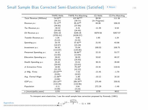
Small Sample Bias Corrected Semi-Elasticities (Satisfied) Return | 55
TWFE Wells TWFE Pre-Matching CS Wells CS Pre-MatchingTotal Revenue (Millions) 74.53** 107.96*** 89.59 111.36
(34.21) (39.71) (In Progress)Revenue p.c. 75.12** 95.43** 84.06 106.03
(34.60) (37.66)Tax Revenue p.c. -30.32 -5.31 -11.39 6.54
(20.58) (24.45)Oil Revenue p.c. 5441.63 6205.26 6679.58 5057.57
(3755.01) (4330.57)Transfer Revenue p.c. 1.26 5.40 1.95 1.24
(5.12) (5.15)Spending p.c. 20.79 37.82** 21.93 43.86
(14.07) (15.18)Investment p.c. 59.35 75.04 180.02 158.75
(113.07) (125.85)Personnel Spending p.c. 14.32 30.86** 22.15 53.77
(12.83) (13.64)Education Spending p.c. 28.02 36.55 33.62 48.37
(26.10) (25.93)Health Spending p.c. 25.42 23.31 38.15 28.69
(29.05) (23.63)# Extractive Firms 18.90 75.28* 23.16 110.61
(31.23) (42.32)# Mfg. Firms -25.03*** -7.53 -21.45 -1.79
(8.05) (8.92)Avg. Formal Wage -11.06** -1.80 -10.12 10.10
(4.66) (4.38)GDP p.c. 253.10** 290.35** 275.49 330.81
(110.29) (116.96)Population -3.11 3.94 272.29 -1.46
(4.49) (4.23)n (municipality-years) 1278 9012 1278 9012
To interpret semi-elasticities, I use the small sample bias correction proposed by Kennedy (1981):
P̂ = (e(β− V̂ar(β)2 ) − 1) × 100Appendices
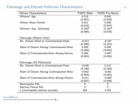
Patronage and Elected Politician Characteristics | 56
Winner Characteristics TWFE Wells TWFE Pre-MatchWinners’ Age 0.118 0.045
(0.691) (0.629)Winner Share Female 0.011 0.008
(0.018) (0.018)Winners’ Avg. Schooling -0.150* -0.142*
(0.089) (0.076)
Patronage (Mayors Only)No. Donors Hired to Commissioned Posts -0.013 -0.197
(0.045) (0.222)Share of Donors Among Commissioned Hires 0.000 0.000
(0.000) (0.003)Share of Commissioned Hires Among Donors 0.000 -0.007
(0.001) (0.005)
Patronage (All Politicians)No. Donors Hired to Commissioned Posts -0.039 0.137
(0.186) (0.169)Share of Donors Among Commissioned Hires -0.002 -0.001
(0.003) (0.003)Share of Commissioned Hires Among Donors -0.011 -0.008
(0.007) (0.006)Municipality FEs Y YElection Period FEs Y Yn (municipality-election periods) 404 3,745
ReturnAppendices
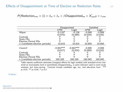
Effects of Disappointment at Time of Election on Reelection Rates | 57
P(Reelectioncme = 1) = δm + λe + βDisappointedme + X ′cmeµ + εcme
Disappointed SatisfiedLPM Logit LPM Logit
Mayor -0.119* -0.136 -0.006 -0.006(0.070) (0.089) (0.034) (0.034)
Controls Y Y Y YState FEs Y Y Y YElection Period FEs Y Y Y Yn (candidate-election periods) 10,815 10,815 10,850 10,850
Council -0.052*** -0.042*** -0.005 -0.008(0.017) (0.016) (0.009) (0.010)
Controls Y Y Y YState FEs Y Y Y YElection Period FEs Y Y Y Yn (candidate-election periods) 160,169 160,169 160,945 160,945
Table reports coefficient estimates (marginal effects for logit models) with standard errors clus-tered at municipality level in parentheses Disappointedme is same indicator used in event studyanalyses, but time-varying. Controls include candidate age, sex, and education level. ***p<0.01, ** p<0.05, * p<0.1
Return
Appendices
Related Documents