The Preferences of the Euro Area Monetary Policymaker &ast

* The authors are members of CEMPRE (Centro de Estudos Macroeconómicos e Previsão, Faculdade de Economia, Universidade do Porto) which is supported by the Fundação para a Ciência e a Tecnologia, Portugal. We thank Fabio Canova and two anonymous referees for comments and suggestions, and Richard Dennis for sharing the Gauss code of his study of the policy preferences of the US Federal Reserve.

JCMS 2005 Volume 43. Number 2. pp. 221–50

© Blackwell Publishing Ltd 2005 9600 Garsington Road, Oxford OX4 2DQ, UK and 350 Main Street, Malden, MA 02148, USA

Abstract

The aim of this article is to uncover the aggregate monetary policy preferences in the euro area. This is pursued under the assumption of optimizing policy behaviour subject to a simple model of the macroeconomic structure, following a procedure proposed recently in the literature in which GMM estimation stems from the optimal control solution to the optimization problem. Instead of waiting for more quarterly data of ECB policy-making, the sample goes as far back as possible into the pre-EMU years. Through a combined analysis of facts, data and literature on European integration, 1995 is identified as the start date of a euro area notional policy regime, sustained later by the ECB. The policy preferences are estimated as a loss function with strict inflation targeting at 1.6 per cent and interest-rate smoothing, in the period 1995–2002.

Introduction

The purpose of this article is to estimate the monetary policy preferences in the aggregate euro area. The loss function of the euro area policy-maker is estimated with data on output gap, inflation, short-term interest rates and imported inflation, assuming an optimizing policy behaviour subject to a macroeconomic structure that can be modelled with a small aggregate-supply and aggregate-demand dynamic model. In addition to the challenging study

The Preferences of the Euro Area Monetary Policy-maker*

ALVARO AGUIAR Universidade do PortoMANUEL M.F. MARTINSUniversidade do Porto

01Ag&Mart221-50*.indd 221 28/4/05 9:44:42 am

222

© Blackwell Publishing Ltd 2005

ALVARO AGUIAR AND MANUEL M.F. MARTINS

of the aggregate euro area case, a more technical contribution of the article is the use of a quasi real-time output gap, notionally closer to the information available to policy-makers when deciding policy, than the official ex post gaps routinely used in the research of, for instance, the preferences of the US Federal Reserve (the Fed).

At this stage it is not yet possible to extract econometrically the parameters of the loss function of the European Central Bank (ECB) because of the scar-city of quarterly data since the launch in January 1999 of European monetary union (EMU), and in view of the shortcomings of monthly data – an excess of volatility and an inability to account parsimoniously for the cyclical condition of the economy.

Instead of waiting for further data on policy-making by the ECB, we extend the estimation period as far back as possible in order to achieve a satisfactory estimation of the policy preferences. That is, in addition to the actual time of the ECB’s operation, we include a previous period during which it is reasonable to consider the group of central banks of the current EMU as if they were a single monetary authority. In this view, the preferences of this notional central bank, founded in 1992 in the consensus over the Maastricht criteria for EMU initial membership, are the driving force behind each country’s monetary policy during the process of successful convergence towards January 1999.

In the time between the Treaty and the actual Union, we determine the beginning of the estimation period – 1995 – through a combination of analy-sis of facts, data and literature. Facts are on European integration, data on the aggregate area and its main countries, and literature on the convergence of macroeconomic structures and cycles in the EMU countries.

The main findings are that this euro area policy-maker sets interest rates to aim at an inflation target of around 1.6 per cent, with no direct concern over output gap stabilization, and significantly smoothing the policy instrument. This result is subject to sensitivity checks concerning the start date of the sample, the procedure for deriving the interest rate equation describing the central bank optimizing behaviour, and the econometric technique used to estimate the model parameters.

The article is outlined as follows. Section I reviews data, facts and literature in order to define the beginning of the sample for estimation of the monetary policy-maker’s preferences, and identifies a stable aggregate demand–aggregate supply structure of the euro area. Section II sets up the optimizing model for monetary policy analysis, explains the estimation procedure, and presents the results for the euro area. In Section III some sensitivity checks are conducted, and the final section concludes.

01Ag&Mart221-50*.indd 222 28/4/05 9:44:43 am

223

© Blackwell Publishing Ltd 2005

THE PREFERENCES OF THE EURO AREA MONETARY POLICY-MAKER

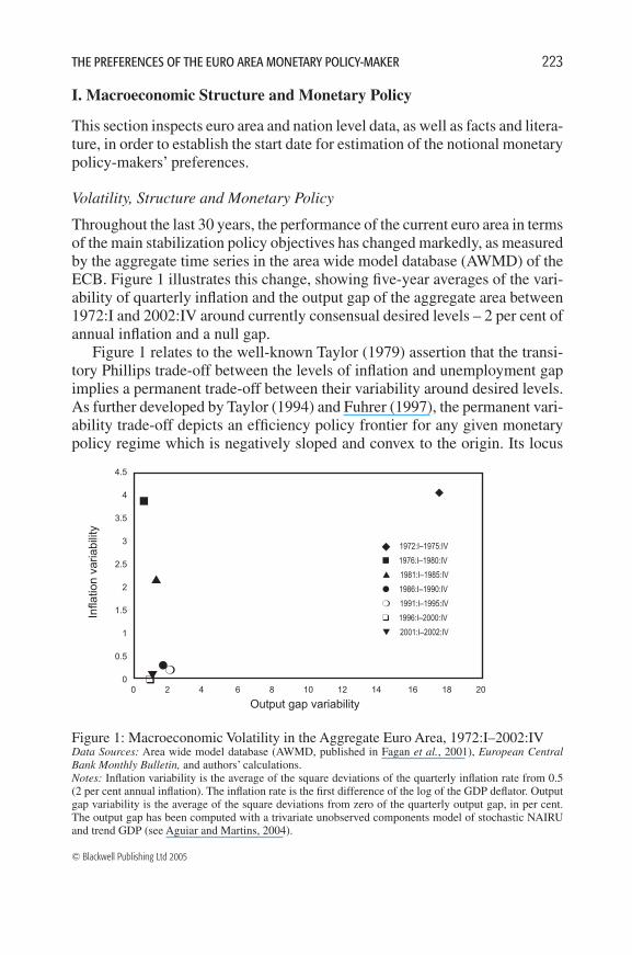
Figure 1: Macroeconomic Volatility in the Aggregate Euro Area, 1972:I–2002:IV Data Sources: Area wide model database (AWMD, published in Fagan et al., 2001), European Central Bank Monthly Bulletin, and authors’ calculations.Notes: Inflation variability is the average of the square deviations of the quarterly inflation rate from 0.5 (2 per cent annual inflation). The inflation rate is the first difference of the log of the GDP deflator. Output gap variability is the average of the square deviations from zero of the quarterly output gap, in per cent. The output gap has been computed with a trivariate unobserved components model of stochastic NAIRU and trend GDP (see Aguiar and Martins, 2004).

I. Macroeconomic Structure and Monetary Policy

This section inspects euro area and nation level data, as well as facts and litera-ture, in order to establish the start date for estimation of the notional monetary policy-makers’ preferences.

Volatility, Structure and Monetary Policy

Throughout the last 30 years, the performance of the current euro area in terms of the main stabilization policy objectives has changed markedly, as measured by the aggregate time series in the area wide model database (AWMD) of the ECB. Figure 1 illustrates this change, showing five-year averages of the vari-ability of quarterly inflation and the output gap of the aggregate area between 1972:I and 2002:IV around currently consensual desired levels – 2 per cent of annual inflation and a null gap.

Figure 1 relates to the well-known Taylor (1979) assertion that the transi-tory Phillips trade-off between the levels of inflation and unemployment gap implies a permanent trade-off between their variability around desired levels. As further developed by Taylor (1994) and Fuhrer (1997), the permanent vari-ability trade-off depicts an efficiency policy frontier for any given monetary policy regime which is negatively sloped and convex to the origin. Its locus

Output gap variability

Infla

tion

varia

bilit

y

4.5

4

3.5

3

2.5

2

1.5

1

0.5

00 2 4 6 8 10 12 14 16 18 20

1972:I–1975:IV

1976:I–1980:IV

1981:I–1985:IV

1986:I–1990:IV

1991:I–1995:IV

1996:I–2000:IV

2001:I–2002:IV

01Ag&Mart221-50*.indd 223 28/4/05 9:44:44 am

224

© Blackwell Publishing Ltd 2005

ALVARO AGUIAR AND MANUEL M.F. MARTINS

depends on the policy regime and on the variability of the shocks hitting the economy, and its slope is a function of the structure of the economy, includ-ing the elasticity of the short-term Phillips curve. The optimal policy choice yields a specific combination in the efficiency frontier, which is a function of the relative weight attached to inflation and activity gap volatility in the policy-maker’s loss function.

Taken at face value, Figure 1 seems to indicate a shift in policy preferences from output stabilization to inflation stabilization during the 1980s, possibly together with some decline of supply shocks, and the existence of a stable regime during the second half of the 1980s and first half of the 1990s target-ing a low rate of inflation. During the second half of the 1990s and the two first years of the twenty-first century, the policy regime and/or the intensity of supply shocks may have changed further, leading the area to remarkably low levels of volatility of both inflation and output gap.

However, whatever the picture suggests, it allows for a coherent interpreta-tion of the aggregate euro area monetary policy preferences only if it is not a spurious result of the aggregation of heterogeneous national macro structures, supply shocks, and/or monetary policy regimes. In this respect, the fact remains that the institutional economic and monetary union of the area Member States exists only since 1999:I, and there seems to be no wide consensus as to when the area’s national economies became homogeneous. In order to determine to what extent – i.e. since when – the information in Figure 1 may actually be read within Taylor’s framework, we now look at national data, the main events of European monetary integration, and results from the literature on convergence of structures and cycles in the area countries. The section then finishes with tests for structural stability of a small macro model for the aggregate area.

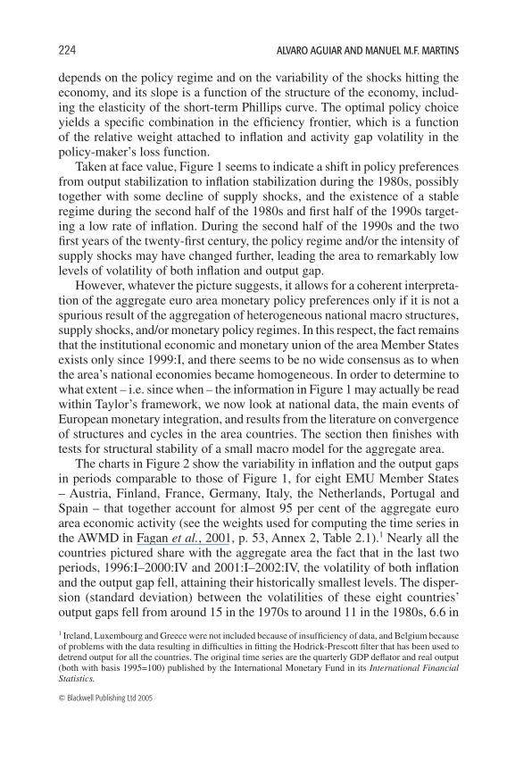
The charts in Figure 2 show the variability in inflation and the output gaps in periods comparable to those of Figure 1, for eight EMU Member States – Austria, Finland, France, Germany, Italy, the Netherlands, Portugal and Spain – that together account for almost 95 per cent of the aggregate euro area economic activity (see the weights used for computing the time series in the AWMD in Fagan et al., 2001, p. 53, Annex 2, Table 2.1).1 Nearly all the countries pictured share with the aggregate area the fact that in the last two periods, 1996:I–2000:IV and 2001:I–2002:IV, the volatility of both inflation and the output gap fell, attaining their historically smallest levels. The disper-sion (standard deviation) between the volatilities of these eight countries’ output gaps fell from around 15 in the 1970s to around 11 in the 1980s, 6.6 in

1 Ireland, Luxembourg and Greece were not included because of insufficiency of data, and Belgium because of problems with the data resulting in difficulties in fitting the Hodrick-Prescott filter that has been used to detrend output for all the countries. The original time series are the quarterly GDP deflator and real output (both with basis 1995=100) published by the International Monetary Fund in its International Financial Statistics.

01Ag&Mart221-50*.indd 224 28/4/05 9:44:44 am

225

© Blackwell Publishing Ltd 2005

THE PREFERENCES OF THE EURO AREA MONETARY POLICY-MAKER

Infla

tion

varia

bilit

y

Output gap variability

2

1.6

1.2

0.8

0.4

0

Netherlands

0 1 2 3 4 5 6 7 8

Infla

tion

varia

bilit

y

Output gap variability

16

14

12

10

8

6

4

2

0

Spain

0 1 2 3 4 5 6 7 8

Infla

tion

varia

bilit

y

Output gap variability

16

14

12

10

8

6

4

2

0

Italy

0 1 2 3 4 5 6 7 8

Figure 2: Macroeconomic Volatility in Euro Area Countries, 1972:I–2002:IVData sources: International Financial Statistics of the International Monetary Fund, and authors’ calcula-tions.Notes: Inflation variability is the average of the square deviations of the quarterly inflation rate from 0.5 (2 per cent annual inflation). The inflation rate is the first difference of the log of the GDP deflator (IFS, 1995 = 100). Output gap variability is the average of the square deviations from zero of the quarterly output gap, in per cent. The gap is the deviation, in per cent, of real output (IFS, 1995 = 100) from its trend, which has been computed with the Hodrick-Prescott filter (λ=1600).

Infla

tion

varia

bilit

y

Output gap variability

32

28

24

20

16

12

8

4

0

Portugal

0 1 2 3 4 5 6 7 8

Infla

tion

varia

bilit

y

Output gap variability

9

8

7

6

5

4

3

2

1

0

Austria

0 10 20 30 40 50

Infla

tion

varia

bilit

y

Output gap variability

25

20

15

10

5

0

Finland

0 5 10 15 20 25 30

Infla

tion

varia

bilit

y

Output gap variability

5

4

3

2

1

0

France

0 1 2 3 4 5 6 7 8 9 10

Infla

tion

varia

bilit

y

Output gap variability

2

1.6

1.2

0.8

0.4

0

Germany

0 1 2 3 4 5 6 7 8 9 10

1972:I–1975:IV 1976:I–1980:IV 1981:I–1985:IV 1986:I–1990:IV 1991:I–1995:IV 1996:I–2000:IV 2001:I–2002:IV

01Ag&Mart221-50*.indd 225 28/4/05 9:44:45 am

226

© Blackwell Publishing Ltd 2005

ALVARO AGUIAR AND MANUEL M.F. MARTINS

1991–95, 3.6 in 1996–2000 and 1.4 in 2001–02. The dispersion between the volatilities of inflation increased up to 10.2 in 1986–90, but then fell sharply to 1.2 in 1991–95, 0.6 in 1996–2000 and 0.4 in 2001–02. Overall, the national data support the pattern shown in Figure 1 for the aggregate euro area. We then conclude that it is not a spurious result, but rather a group one, at least since the mid-1990s.

The events in European integration further strengthen our conclusion of harmonization in national level macroeconomic volatilities during the 1990s. Throughout the first half of the 1990s, the European single market has been deepening economic integration between the Union Member States. Since March 1995 there has been no parity realignment in the exchange-rate mecha-nism of the European monetary system, and the actual fluctuation of market exchange rates inside their theoretical bands has been almost imperceptible, especially since 1996. Given that capital movements in the European Union had been fully liberalized by 1992, exchange rate stability means that monetary policy has de facto been unified since the mid-1990s.

The recent literature on the synchronization of business cycles in the euro area seems to confirm a significant economic harmonization within the area. Agresti and Mojon (2001) find that national level cycles of quarterly real GDP are positively correlated with the aggregate area cycle throughout 1972–98, with increased significance since the mid-1990s. Luginbuhl and Koopman (2004) model the convergence in per capita real GDP of Germany, France, Italy, Spain and the Netherlands as a gradually evolving unobserved variable, and find that the growth component converged by 1985, the cycle component converged by 1990, and the overall variance had reached half of convergence by 1995. Artis et al. (2004) find high correlations between the smoothed probabilities of changes in the growth rate of monthly industrial production of the individual area countries, except for the UK, during the last three decades of the twentieth century, and estimate an aggregate area cycle. Artis et al. (2005) compare results from several alternative methods and time series, and find a systematic tendency for the cross-sectional disper-sion of the industrial production cycles of the area countries to shrink over time, arriving at very low dispersions during the second half of the 1990s.

The analysis so far suggests that a common macroeconomic structure for the aggregate euro area may have been well defined since the mid-1990s. Since its stability is a necessary condition for the purpose of identifying the monetary policy regime in the absence of a single monetary authority, we now proceed sequentially. First, in the rest of this section, we formulate a small dynamic macro model and test its stability with euro area data from 1972 until 2002, in order to determine the start date of a stable structure. Then, in Section II, with the sample period appropriately restricted to this start date, we are able to test

01Ag&Mart221-50*.indd 226 28/4/05 9:44:46 am

227

© Blackwell Publishing Ltd 2005

THE PREFERENCES OF THE EURO AREA MONETARY POLICY-MAKER

for the existence of a notional policy regime by simultaneously identifying both the policy-makers’ preferences and the macroeconomic structure.

Aggregate Demand – Aggregate Supply

The structure of the euro area aggregate economy is modelled as a simple backward-looking aggregate demand–aggregate supply system similar to that applied by Rudebusch and Svensson (1999) to US data, where aggregate de-mand is an IS equation expressed in terms of output gap, and aggregate supply is an expectations augmented Phillips equation.

Rudebusch and Svensson’s motivation for using this model was threefold: the tractability and transparency of results; a good fit to recent US data; and the proximity to many policy-makers’ views about the dynamics of the economy, and to the spirit of many policy-oriented macroeconometric models, including some used by central banks. In addition, we have two reasons of our own.

First, it has been widely used in recent empirical studies of monetary policy rules or regimes as in, inter alia, Favero and Rovelli (2003), Dennis (2003) and, for European countries, Peersman and Smets (1999), Taylor (1999) and Aksoy et al. (2002). While the intensive use does not necessarily mean that the model entirely represents the structure of actual developed economies, it does, however, reflect its sensible theoretical and empirical properties, from which Goodhart (2001) stresses the realistic inclusion of monetary transmis-sion lags.

Second, even though most of the uses of the model relate to the US, it seems reasonable to expect the structure of the euro area to be broadly similar, since both are large and relatively closed economies – as argued, for instance, by Rudebusch and Svensson (2002). In support of this belief, Agresti and Mojon (2001) find that the business cycle of the aggregate euro area is similar to the US in several respects, and Angeloni et al. (2003) show that the responses of the area’s output and inflation to monetary actions are quite close to those typically reported for the US. In fact, both Peersman and Smets (1999) and Taylor (1999) have successfully estimated this model with aggregate data of a core of EMU countries. Moreover, our assumption that the euro area may be studied following approaches already used for the US economy is also backed by analysis from alternative theoretical frameworks. For instance, Smets and Wouters (2004) estimate a dynamic structural general equilibrium model for both the US and the euro area over 1974–2002, finding remarkably similar characteristics in the two areas concerning the type of shocks, their propagation mechanisms, and the responses of monetary policy to shocks. Following a thorough process using standard model identification criteria, we assume the following specific version of the Rudebusch-Svensson model:

01Ag&Mart221-50*.indd 227 28/4/05 9:44:46 am

228

© Blackwell Publishing Ltd 2005

ALVARO AGUIAR AND MANUEL M.F. MARTINS

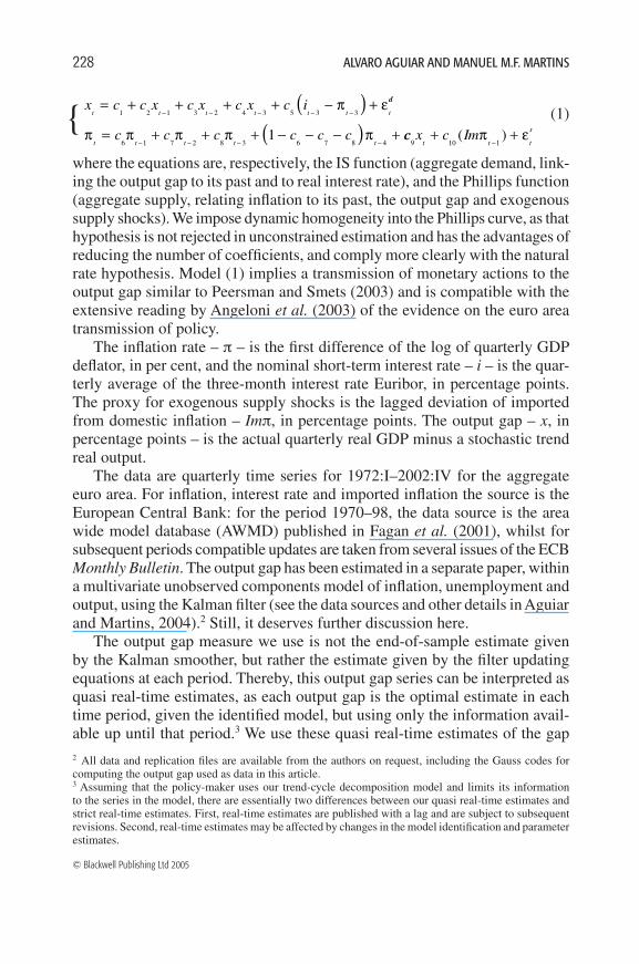
(1)

where the equations are, respectively, the IS function (aggregate demand, link-ing the output gap to its past and to real interest rate), and the Phillips function (aggregate supply, relating inflation to its past, the output gap and exogenous supply shocks). We impose dynamic homogeneity into the Phillips curve, as that hypothesis is not rejected in unconstrained estimation and has the advantages of reducing the number of coefficients, and comply more clearly with the natural rate hypothesis. Model (1) implies a transmission of monetary actions to the output gap similar to Peersman and Smets (2003) and is compatible with the extensive reading by Angeloni et al. (2003) of the evidence on the euro area transmission of policy.

The inflation rate – π – is the first difference of the log of quarterly GDP deflator, in per cent, and the nominal short-term interest rate – i – is the quar-terly average of the three-month interest rate Euribor, in percentage points. The proxy for exogenous supply shocks is the lagged deviation of imported from domestic inflation – Imπ, in percentage points. The output gap – x, in percentage points – is the actual quarterly real GDP minus a stochastic trend real output.

The data are quarterly time series for 1972:I–2002:IV for the aggregate euro area. For inflation, interest rate and imported inflation the source is the European Central Bank: for the period 1970–98, the data source is the area wide model database (AWMD) published in Fagan et al. (2001), whilst for subsequent periods compatible updates are taken from several issues of the ECB Monthly Bulletin. The output gap has been estimated in a separate paper, within a multivariate unobserved components model of inflation, unemployment and output, using the Kalman filter (see the data sources and other details in Aguiar and Martins, 2004).2 Still, it deserves further discussion here.

The output gap measure we use is not the end-of-sample estimate given by the Kalman smoother, but rather the estimate given by the filter updating equations at each period. Thereby, this output gap series can be interpreted as quasi real-time estimates, as each output gap is the optimal estimate in each time period, given the identified model, but using only the information avail-able up until that period.3 We use these quasi real-time estimates of the gap 2 All data and replication files are available from the authors on request, including the Gauss codes for computing the output gap used as data in this article.3 Assuming that the policy-maker uses our trend-cycle decomposition model and limits its information to the series in the model, there are essentially two differences between our quasi real-time estimates and strict real-time estimates. First, real-time estimates are published with a lag and are subject to subsequent revisions. Second, real-time estimates may be affected by changes in the model identification and parameter estimates.

x c c x c x c x c it t t t t t t

= + + + + − +− − − − −( )

1 2 1 3 2 4 3 5 3 3π εdd

t t t t tc c c c c cπ π π π π= + + + − − − +

− − − −( )6 1 7 2 8 3 6 7 8 4

1 cc x c Imt t t

s

9 10 1+ +

−( )π ε

01Ag&Mart221-50*.indd 228 28/4/05 9:44:48 am

229

© Blackwell Publishing Ltd 2005

THE PREFERENCES OF THE EURO AREA MONETARY POLICY-MAKER

because they are conceptually closer to the policy-makers’ real-time perceptions of the state of the economy than the ex post official gap series available at the time of research that have typically been used by researchers estimating the US Federal Reserve policy preferences, like Favero and Rovelli (2003) and Dennis (2003).

Our preference for using gap estimates as close as possible to real-time data is motivated by recent literature showing that the assumptions about the timing of information-gathering can be quite relevant for policy analysis. The impor-tance of using data available to policy-makers in real time in ex post evaluations of monetary policy has been shown, for the US, by Orphanides (2001, 2002). Nelson and Nikolov (2003) also report a pattern of official real-time output gap misperceptions in the UK during the 1970s similar to that identified by Orphanides for the US. In both cases, the authors inspected the information actually used at the meetings of monetary policy committees.

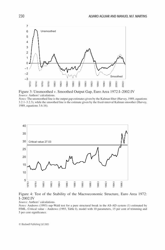
Here, however, we cannot use proper real-time information, because, for almost the whole sample period, there is no aggregate euro area real-time sta-tistical data and we are evaluating the policy of a notional central bank.4 Hence the option for using the quasi real-time approach explained above. Figure 3 illustrates, for our case, the discrepancies between ex post and quasi real-time estimates, showing the output gap series given by the Kalman smoother and the series given by the Kalman filter.

In order to determine the start date of a stable macroeconomic structure in the euro area we test the stability of system (1) over the entire sample. As there is no precise a priori indication about the timing of possible structural breaks, one appropriate test is based on Andrews (1993, equations 4.1 and 4.2) sup-Wald statistic. Figure 4 reports the results of this test, for a joint full information maximum likelihood (FIML) estimation of the system with the standard 15 per cent trimming. The null hypothesis of no structural change is rejected, at the usual significance level of 5 per cent.

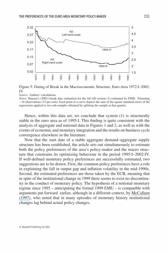
Next, we set out to estimate the dates of structural break. Due to the well-known problems with the Wald test for such a task, we follow Hansen’s (2001) suggestion, which consists of identifying the sample split that minimizes the sum of the standard errors of the regressions of the two sub-samples, before and after the break date. As Figure 5 shows, it turns out that the dates of struc-tural breaks in both the IS and the Phillips equation are estimated at near the end of 1994 – respectively 1994:IV and 1994:III – with no signs of any other breaks.

4 Coenen et al. (2005) study the profile of revision of the main macroeconomic variables in the euro area during 1999 and 2000, using the numbers published in the ECB Monthly Bulletin – an approach that may prove to be very helpful in future research on EMU policy-making with real-time data.

01Ag&Mart221-50*.indd 229 28/4/05 9:44:49 am

230

© Blackwell Publishing Ltd 2005

ALVARO AGUIAR AND MANUEL M.F. MARTINS

Unsmoothed

Smoothed

Figure 3: Unsmoothed v. Smoothed Output Gap, Euro Area 1972:I–2002:IVSource: Authors’ calculations.Notes: The unsmoothed line is the output gap estimates given by the Kalman filter (Harvey, 1989, equations 3.2.1–3.2.3), while the smoothed line is the estimate given by the fixed-interval Kalman smoother (Harvey, 1989, equations 3.6.16).

7

6

5

4

3

2

1

0

–1

–2

–3

1972

:I

1974

:I

1976

:I

1978

:I

1980

:I

1982

:I

1984

:I

1986

:I

1988

:I

1990

:I

1992

:I

1994

:I

1996

:I

1998

:I

2000

:I

2002

:I

Figure 4: Test of the Stability of the Macroeconomic Structure, Euro Area 1972:I–2002:IVSource: Authors’ calculations.Notes: Andrews (1993) sup-Wald test for a pure structural break in the AS-AD system (1) estimated by FIML. Critical value – Andrews (1993, Table I), model with 10 parameters, 15 per cent of trimming and 5 per cent significance.

1976

:I

1978

:I

1980

:I

1982

:I

1984

:I

1986

:I

1988

:I

1990

:I

1988

:I

1990

:I

1992

:I

1994

:I

1996

:I

40

35

30

25

20

15

10

5

Critical value 27.03

01Ag&Mart221-50*.indd 230 28/4/05 9:44:59 am

231

© Blackwell Publishing Ltd 2005

THE PREFERENCES OF THE EURO AREA MONETARY POLICY-MAKER

Hence, within this data set, we conclude that system (1) is structurally stable in the euro area as of 1995:I. This finding is quite consistent with the analysis of aggregate and national data in Figures 1 and 2, as well as with the events of economic and monetary integration and the results on business cycle convergence elsewhere in the literature.

Now that the start date of a stable aggregate demand–aggregate supply structure has been established, the article sets out simultaneously to estimate both the policy preferences of the area’s policy-maker and the macro struc-ture that constrains its optimizing behaviour in the period 1995:I–2002:IV. If well-defined monetary policy preferences are successfully estimated, two suggestions are to be drawn. First, the common policy preferences have a role in explaining the fall in output gap and inflation volatility in the mid-1990s. Second, the estimated preferences are those taken by the ECB, meaning that in spite of the institutional change in 1999 there seems to exist no discontinu-ity in the conduct of monetary policy. The hypothesis of a notional monetary regime since 1995 – anticipating the formal 1999 EMU – is compatible with arguments put forward earlier, although in a different context, by McCallum (1997), who noted that in many episodes of monetary history institutional changes lag behind actual policy changes.

Figure 5: Dating of Break in the Macroeconomic Structure, Euro Area 1972:I–2002:IVSource: Authors’ calculations.Notes: Hansen’s (2001) break-date estimation for the AS-AD system (1) estimated by FIML. Trimming – 16 observations (15 per cent). Each point in a curve depicts the sum of the square standard errors of the regressions applied to two sub-samples obtained by splitting the sample at that quarter.

1994:IV

0.32

0.27

0.22

0.17

0.12

0.07

0.02

5

4.5

4

3.5

3

2.5

2

1.5

ADLeft-hand scale

ASRight-hand scale

1994:III

1976

:I

1978

:I

1980

:I

1982

:I

1984

:I

1986

:I

1988

:I

1990

:I

1992

:I

1994

:I

1996

:I

1998

:I

01Ag&Mart221-50*.indd 231 28/4/05 9:45:06 am

232

© Blackwell Publishing Ltd 2005

ALVARO AGUIAR AND MANUEL M.F. MARTINS

II. Estimating the Policy Preferences of the Euro Area Policy-maker

In this section, after specifying the central bank loss function, the optimiza-tion problem faced by the policy-maker, and its solution are presented. Then, the econometric technique is described, and the main results are reported. We follow Favero and Rovelli (2003) deriving the optimality conditions for the policy instrument – short-term interest rate – using optimal control, and then jointly estimating the interest rate equation with the dynamic macro structure of the economy by the generalized method of moments (GMM). Finally, the interest rate path implied by the estimated model is compared to the actual path and to that implied by a standard formulation of the Taylor rule.

Central Bank Preferences

Following fairly standard assumptions in the literature, we model the central bank’s preferences as an intertemporal loss functional. In each period the loss function is quadratic in the deviations of inflation and the output gap from desired levels (π* and 0, respectively), as well as in the change in the interest rate, which is the policy instrument. Future values are discounted at rate δ, and the weights λ and μ are non-negative.

(2)

The inclusion of the output gap variability in L is generally considered com-patible with the statutes of modern central banks, such as the US Fed. Even inflation targeting regimes, which have a formally quantified commitment to price stability, have a second order objective concerning growth and employ-ment (see Svensson, 2003). However, the ECB statutes, similarly to those of the Bundesbank, are not entirely clear about the significance that real activity stabilization has in its legal mandate, as they merely state in the second article of its Chapter II, concerning the European system of central banks (ESCB), that

the primary objective of the ESCB shall be to maintain price stability. With-out prejudice to the objective of price stability it shall support the general economic policies in the Community. (ECB, 2002, p. 2)

The ECB Governing Council, when announcing its stability-oriented monetary policy strategy, established that

As mandated by the Treaty establishing the European Community, the maintenance of price stability will be the primary objective of the ESCB. Therefore, the ESCB’s monetary policy strategy will focus strictly on this objective. (ECB, 1998, Article 2)

L E x i it t t t t t

= ∑ − + + −=

∞

+ + + + −( )δ π π λ µτ

ττ τ τ τ

0

2 21

2*

11

2( )

01Ag&Mart221-50*.indd 232 28/4/05 9:45:08 am

233

© Blackwell Publishing Ltd 2005

THE PREFERENCES OF THE EURO AREA MONETARY POLICY-MAKER

This has led some authors (e.g. Goodhart, 1998) to argue that output is not supposed to form part of the true ECB objective function. In general, McCal-lum (2001a) also argues that, for uncertainty reasons, monetary policy should not respond strongly to output gaps. Summed up, we specify our baseline loss, L, as a flexible inflation targeting regime, which nests the strict inflation targeting case – no concern with the variance of the gap – letting the evidence determine which of these systems better fits the revealed preferences of the euro area policy-maker.

In what concerns the inclusion of the changes in the interest rate, we fol-low a relatively standard practice in the empirically oriented literature, which is to consider that the policy-maker also dislikes variations in the policy instrument – the so-called interest-rate smoothing. Even though theoretical central bank loss functions do not include the instrument as part of the final goals of policy, the fact is that optimal interest rates simulated from models with such loss functions are substantially more volatile than actual short-term interest rates (see Sack, 2000). Central banks tend to change interest rates in small discrete steps and reverse their path infrequently (for a review, see Sack and Wieland, 2000).5 Although several authors have argued that the evidence of policy inertia has little structural content, mostly reflecting econometric problems (see, e.g., Rudebusch, 2002), recent simulations and estimations in Favero (2001) and English et al. (2003) reiterate the evidence in favour of intentional smoothing.

Before proceeding to the optimization solution and the estimation, a brief reference to the exclusion of money and exchange rates is in order. Following the currently consensual monetary policy analysis framework (see McCal-lum, 2001b), no monetary aggregate is included in our model, implying that money is neither an instrument nor an intermediate target of policy.6 As a re-sult, however, the estimates should be interpreted with some caution, since no distinction between money supply and money demand surfaces in the model and, thus, some coefficients may be reflecting mixed effects from demand and policy changes.

As for the absence of an exchange-rate variable as an intermediate or final target, this is grounded in two arguments. On the one hand, exchange rates are likely to matter less in a policy rule of a large and relatively closed economy like the euro area than in a small open economy (see Peersman and Smets, 1999). On the other hand, the evidence in Clarida and Gertler (1997) indicates that the Bundesbank’s concerns with the DMark exchange rate when conducting

5 Further motivations for interest-rate smoothing have been put forward by Goodhart (2001) and Rudebusch (2002).6 This is seemingly at odds with the ECB first pillar, which covers monetary aggregate growth targeting (see ECB, 1998). However, several recent studies have found no evidence that money has been relevant in the ECB’s policy decisions (Mihov, 2001; Begg et al., 2002).

01Ag&Mart221-50*.indd 233 28/4/05 9:45:08 am

234

© Blackwell Publishing Ltd 2005

ALVARO AGUIAR AND MANUEL M.F. MARTINS

monetary policy were essentially related to its importance as a determinant of domestic inflationary pressures rather than as a final target per se. This seems to be the case for the ECB as well, as put forward recently by Gaspar and Iss-ing (2002). And this role of the exchange rate as determinant of inflationary pressures is already implicitly considered in our model through the lagged deviation of imported from domestic inflation.

Estimating Policy-makers’ Preferences

For the sake of realism and estimation feasibility, we circumscribe the opti-mization problem to a discretionary policy regime, in line with Rudebusch and Svensson (1999) and, indeed, with much of the empirical research. In this regime, the policy-maker solves for the optimal closed-loop system, i.e. sets its policy sequentially, in each period, given the then observed state of the economy. In this case, the monetary authority chooses in each period the interest rate that minimizes the intertemporal loss functional subject to the dynamic economic structure:

(3)

subject to system (1).As the policy control variable is the short-term interest rate, the solution

is an expression describing the optimal interest rate as a function of the state variables of the system. Once supplemented by an innovation, that expression joins the system describing the dynamics of the economy, and estimation of the structural parameters of the model may be carried out.

The approach devised by Favero and Rovelli (2003) is based on the Euler equation of the system – the first-order condition – which in this case takes the form

(4)

This equation is then truncated at four quarters ahead, and the partial derivatives in it are expanded and written as a function of the relevant aggregate-supply and aggregate-demand coefficients in (1). At this stage, the expression of the first-order condition conveniently includes the cross-equation restrictions of the system, ensuring that the loss function is properly minimized subject to the constraints given by the economy structure. Further supplemented with an innovation, the Euler equation, in estimation form, becomes

Ei

Et t

t

t

tδ π π

πδ λτ

ττ

τ τ

τ=

∞

+

+

=

∞

∑ −∂

∂+ ∑

0 0

( *) xxx

i

i i E i i

t

t

t

t t t t t

+

+

− +

∂

∂

+ − − −

τ

τ

µ µδ( ) (1 1

))[ ] = 0

Min L Min E xt t t t

it

( ) *= ∑ − + +=

∞

+ +( )δ π π λ µτ

ττ τ

1

20

2 2 ii i tt t+ + −

− ∀( )

τ τ 1

2

,

01Ag&Mart221-50*.indd 234 28/4/05 9:45:11 am

235

© Blackwell Publishing Ltd 2005

THE PREFERENCES OF THE EURO AREA MONETARY POLICY-MAKER

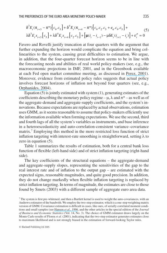
(5)

Favero and Rovelli justify truncation at four quarters with the argument that further expanding the horizon would complicate the equation and bring col-linearities to the system, causing great difficulties to estimation. We argue, in addition, that the four-quarter forecast horizon seems to be in line with the forecasting needs and abilities of real world policy-makers (see, e.g., the macroeconomic projections in IMF, 2001, and in the Greenbook available at each Fed open market committee meeting, as discussed in Perez, 2001). Moreover, evidence from estimated policy rules suggests that actual policy involves forecast horizons of inflation not beyond four quarters (see, e.g., Orphanides, 2004).

Equation (5) is jointly estimated with system (1), generating estimates of the coefficients describing the monetary policy regime – μ, λ and π* – as well as of the aggregate-demand and aggregate-supply coefficients, and the system’s in-novations. Because expectations are replaced by actual observations, estimation uses GMM, as it seems reasonable to assume that policy-makers efficiently use the information available when forming expectations. We use the second, third and fourth lags of all the system’s variables as instruments, and base inference in a heteroescedasticity and auto-correlation-consistent variance–covariance matrix.7 Employing this method in the more restricted loss function of strict inflation targeting with interest-rate smoothing is straightforward, setting λ to zero in equation (5).

Table 1 summarizes the results of estimation, both for a central bank loss function of flexible (left-hand side) and of strict inflation targeting (right-hand side).

The key coefficients of the structural equations – the aggregate-demand and aggregate-supply slopes, representing the sensitivities of the gap to the real interest rate and of inflation to the output gap – are estimated with the expected signs, reasonable magnitudes, and quite good precision. In addition, they do not change markedly when flexible inflation targeting is replaced by strict inflation targeting. In terms of magnitude, the estimates are close to those found by Smets (2003) with a different sample of aggregate euro area data.

7 The system is first pre-whitened, and then a Bartlett kernel is used to weight the auto-covariances, with an Andrews estimator of the bandwith. We employ the two-step estimator, which is a one-step weighting matrix version of GMM. Covariance estimation is difficult in cases, like ours, of serially correlated moment condi-tions and small samples (see Hansen et al., 1996, and the other articles in the special edition of the Journal of Business and Economic Statistics (Vol. 14, No. 3). The choice of GMM estimator draws largely on the Monte Carlo results of Floren et al. (2001), indicating that the two-step estimator generates estimates close to maximum likelihood and is not strongly biased in the estimation of forward-looking Taylor rules.

δ π π δ π π33 9 5

44 9 2 5

E c c E c c ct t t t( *) . ( *) . .+ +− + − +[ ] cc c c

E x c E x c ct t t t

6 9 5

33 5

44 2 5

. .

.

[ ][ ] [ ]

+

+ ++ +λδ λδ µµ µδ ε( ) ( )i i E i it t t t t t

p− − − + =− +[ ]1 10

01Ag&Mart221-50*.indd 235 28/4/05 9:45:13 am

236

© Blackwell Publishing Ltd 2005

ALVARO AGUIAR AND MANUEL M.F. MARTINS

The real equilibrium interest rate – r* given by c1/(–c

5) – is estimated at

around 2.1 per cent, which is compatible with the conventional wisdom on the long-run economic growth attainable in the euro area.

As to the parameters revealing the preferences of the monetary policy-maker, the inflation target – π* – and the relative weight of interest-rate smoothing – μ – are reasonably and precisely estimated. In contrast, the weight of the output gap in the loss function – λ in the left-hand side of Table 1 – is not statistically

Table 1: Macroeconomic Structure and Policy-maker’s Loss Function Euro Area 1995:I–2002:IV

Flexible Inflation Targeting Strict Inflation Targeting with Interest-rate smoothing with Interest-rate smoothing Estimates T-stats P-values Estimates T-stats P-values

AD

c1 0.183 5.35 0.00 0.180 5.83 0.00

c2 1.672 18.87 0.00 1.721 25.00 0.00

c3 –0.540 –5.29 0.00 –0.530 –5.20 0.00

c4 –0.241 –5.14 0.00 –0.291 –6.26 0.00

c5 –0.088 –6.25 0.00 –0.084 –6.74 0.00

σ(εd) 0.256 0.260

AS

c6 0.460 4.78 0.00 0.438 6.56 0.00

c7 –0.127 –1.63 0.11 –0.082 –1.16 0.25

c8 0.381 6.55 0.00 0.380 6.66 0.00

c9 0.136 2.75 0.01 0.145 3.16 0.00

c10

0.164 9.00 0.00 0.170 9.60 0.00

σ(εs) 1.123 1.147

CB loss

π* 1.496 9.95 0.00 1.640 12.62 0.00

λ –0.026 –0.74 0.46 – – –

μ 0.028 1.88 0.06 0.030 2.28 0.03 σ(εp) 0.034 0.034

r* 2.069 2.142

J statistic 0.612 19.57 0.81 0.704 22.52 0.71

Source: Authors’ calculations. Notes: Discount factor – δ = 0.975. Optimal control solution – (two-step) GMM estimation. HAC variance–covariance matrix – pre-whitening, Bartlett kernel, Andrews bandwidth. P-values – two-sided significance probabilities. J statistic – value function (1st column), × nobs (2nd column). εp – residuals of the Euler equation. Instruments – constant, Δπ

t–i, x

t–i, i

t–i, Imπ

t–i, i=2, 3, 4.

01Ag&Mart221-50*.indd 236 28/4/05 9:45:14 am

237

© Blackwell Publishing Ltd 2005

THE PREFERENCES OF THE EURO AREA MONETARY POLICY-MAKER

significant. Thus, the hypothesis of flexible inflation targeting is rejected in favour of strict inflation targeting.

In short, this model successfully extracts the preferences of the euro area policy-maker throughout 1995–2002 – inflation targeting at around 1.6 percent-age points, no direct concern for stabilization of the output gap, and significant smoothing of the policy instrument. The standard error of the inflation target means that a 95 per cent confidence interval comprises inflation rates between 1.4 and 1.9 per cent, which is clearly compatible with the ECB’s definition of price stability – inflation below but close to 2 per cent. The failure to reject λ = 0 is very much consistent with the text of Article 2 in ECB (1998), cited above, suggesting that policy has indeed been focusing strictly on price stability.

Assessing the Implied Policy-makers’ Behaviour

We now conduct two simple exercises aimed at improving the understanding of what the estimation results mean as regards the behaviour of the policy-maker.

First, we solve the model dynamically – i.e. performing multi-step forecasts using historical data for lagged endogenous variables (output gap, inflation and interest rates) dated prior to 1995:I and the model’s forecasts thereafter. As Figure 6 shows, the model is stable and replicates quite well the actual path of the interest rate.

Second, we estimate the now standard forward-looking Taylor rule with partial adjustment developed by Clarida et al. (1998).

(6)

using the same set of instruments and GMM estimator as in Table 1, in order to compare its policy outcomes with the behaviour implied by our model. We then solve the Taylor rule dynamically, and evaluate the implied path of the interest rate, which is shown in Figure 6. The Taylor rule does not mimic the actual path as well as our model, scoring a root of mean square error of 0.67, against 0.65.

III. Sensitivity Checks

This section reports several sensitivity exercises to which we have submitted the results, concerning, firstly, the start date of the notional monetary policy regime; secondly, an alternative quasi real-time output gap; thirdly, the exten-sion of the truncation of leads in the Euler equation; fourthly, an alternative method of solution and estimation; and, finally, the central bank loss functions without interest-rate smoothing.

r xt t

e

t

e

tt= − + − + − +

+( ) ( )( ) ( ) / ( ) /1 1 14

ρ α ρ β π ρ γ ρΩ Ω rrt t−

+1

ν

01Ag&Mart221-50*.indd 237 28/4/05 9:45:15 am

238

© Blackwell Publishing Ltd 2005

ALVARO AGUIAR AND MANUEL M.F. MARTINS

Sensitivity to the Date of Emergence of the Monetary Policy Regime

In view of the non-institutional basis for identification of 1995:1 as the start date of the euro area notional policy regime, it is prudent to check the sensi-tivity of the preferences parameters to changes in the starting quarter of the sample period.

Figure 7 shows the main results for all possible samples ending in 2002:IV and starting in 1992:I–1995:IV. The check does not proceed after 1995:IV due to the reduced number of observations.

The first chart in the figure reveals that the weight of interest-rate smooth-ing in the central bank loss function, μ, is not well estimated before 1994:IV. In the samples beginning at that and subsequent quarters, the p-value remains within acceptable levels and the estimates concentrate in the short range from 0.0265 to 0.03.

The second chart in Figure 7 – which does not picture the p-values because the estimates are always significant – shows the inflation target oscillating around 1.6 in the samples beginning at 1993:I and thereafter. The apparent decline of the inflation target estimates throughout the samples beginning between 1992:I and 1993:I suggests that the framework has a good capability of capturing the intensity of the disinflation policies towards EMU in the first half of the 1990s.

Figure 6: Fitted and Actual Interest Rate, Euro Area 1995:I–2002:IVData sources: Area wide model database (AWMD), published in Fagan et al. (2001), European Central Bank Monthly Bulletin, and authors’ calculations.Notes: Optimal policy reaction – interest rates computed by solving the model shown in the right-hand-side of Table 1. Forward-looking Taylor rule – interest rates computed by solving the estimate of equation (6).

8

7

6

5

4

3

2

1

0

1995

:I

1995

:III

1996

:I

1996

:III

1997

:I

1997

:iii

1998

:I

1998

:III

1999

:I

1999

:III

2000

:I

2000

:III

2001

:I

2001

:III

2000

2:I

2002

:III

Actual interest rate

Optimal policy reaction

Forward-looking Taylor rule•

01Ag&Mart221-50*.indd 238 28/4/05 9:45:22 am

239

© Blackwell Publishing Ltd 2005

THE PREFERENCES OF THE EURO AREA MONETARY POLICY-MAKER

Overall, the checks in Figure 7 essentially imply that we could not have begun our sample period more than a quarter before 1995:I, and that if we had chosen to begin estimation at 1994:IV or any of the subsequent quarters

Figure 7: Sensitivity to the Start Date of the Notional Monetary Policy Regime in the Euro AreaSource: Authors’ data. Notes: The dates are the beginnning of each sample period, which ends in 2002:IV. Solution-estima-tion method – see notes to Table 1.

1992:II1992:III

1994:I

1994:II1992:I

1993:I

1992:IV 1993:IV

1993:III1993:II 1994:III

1995:IV 1995:III

1995:II1994:IV

1995:I

1.0

0.9

0.8

0.7

0.6

0.5

0.4

0.3

0.2

0.1

–0.025 –0.02 –0.15 –0.01 –0.005 0 0.005 0.01 0.15 0.02 0.025 0.03 0.035

μ estimate

p-va

lue

A. Interest-rate smoothing

B. Inflation target

1.84

1.78

1.74

1.73

1.62

1.60

1.65

1.61

1.55

1.60

1.631.63

1.64

1.53

1.58

π* e

stim

ate

1992

:I

1992

:II

1992

:III

1992

:IV

1993

:I

1993

:II

1993

:III

1993

:IV

1994

:I

1994

:II

1994

:III

1994

:IV

1995

:I

1995

:II

1995

:III

1995

:IV

1.60

01Ag&Mart221-50*.indd 239 28/4/05 9:45:36 am

240

© Blackwell Publishing Ltd 2005

ALVARO AGUIAR AND MANUEL M.F. MARTINS

through 1995:IV, the estimated policy preferences would be quite similar to those in Table 1.

Sensitivity to Alternative Quasi Real-time Output Gap

As explained in Section I above, our output gap measure has been estimated in a multivariate model comprising information not only on output but also on inflation and unemployment. We now check whether results would change substantially with a – perhaps more conventional – univariate measure of the output cycle. In order to maintain its quasi real-time characteristic, we estimate the output gap with the Kalman filter, within a univariate local linear trend unobserved components model. As this model is affected by the so-called ‘pile-up’ problem, we use Stock and Watson’s (1998) procedure for unbiased estimation of the variance of the trend growth rate.

Table 2 displays the results of the joint estimation of the macroeconomic structure and the policy-makers’ preferences with this univariate gap. While differing from Table 1, the estimates of the IS and Phillips elasticities maintain the correct signs, reasonable magnitudes, and significance. As before, flexible inflation targeting is rejected, at 5 per cent, and the inflation target is estimated at around 1.6 per cent. Thus, as long as its quasi real-time feature is maintained, the use of a univariate – instead of trivariate – output gap does not compromise the previous identification of the policy-makers’ preferences.

Sensitivity to Truncation of Euler Equation

The optimal control solution to the policy-maker’s optimization problem yields an Euler equation that requires lead truncation in order to be usable in estimation. In Section II above, truncation has been set at four quarters ahead – i.e. τ = 0, … , 4 in equation (4) – invoking both Favero and Rovelli’s (2003) pragmatic argument and additional motivations from actual policy-making. As our sample is smaller than Favero and Rovelli’s, the econometric difficulties that they mention for τ > 4 are likely to affect our estimation as well, perhaps even more strongly. Yet, we test the sensitivity of the results to an increase in the truncation horizon of the Euler equation – until six quarters.

Expanding the Euler equation accordingly – describing the behaviour of policy-makers that sets interest rates reacting to output gaps and inflation forecasted up until six quarters ahead – leads to8

8 Comparing equations (7) and (5), one can foresee the econometric difficulties to be expected, due to the number and non-linear combinations of parameters.

01Ag&Mart221-50*.indd 240 28/4/05 9:45:37 am

241

© Blackwell Publishing Ltd 2005

THE PREFERENCES OF THE EURO AREA MONETARY POLICY-MAKER

Table 2: Sensitivity to Univariate Output Gap

Flexible Inflation Targeting Strict Inflation Targeting with Interest-rate smoothing with Interest-rate smoothing Estimates T-stats P-values Estimates T-stats P-values

AD

c1 0.059 3.29 0.00 0.059 3.06 0.00

c2 1.426 15.10 0.00 1.444 16.50 0.00

c3 –0.543 –5.11 0.00 –0.548 –5.27 0.00

c4 0.011 0.22 0.82 0.011 0.19 0.85

c5 –0.024 –3.62 0.00 –0.023 –3.28 0.00

σ(εd) 0.107 0.108

AS

c6 0.419 6.72 0.00 0.390 5.75 0.00

c7 –0.205 –2.53 0.01 –0.157 –2.00 0.05

c8 0.481 4.94 0.00 0.443 4.73 0.00

c9 0.227 1.99 0.05 0.232 1.98 0.05

c10

0.105 6.17 0.00 0.104 6.22 0.00

σ(εs) 1.010 1.007

CB loss

π* 1.778 12.57 0.00 1.616 14.87 0.00

λ –0.308 –1.90 0.06 – – –

μ 0.018 1.82 0.07 0.016 2.21 0.03

σ(εp) 0.015 0.014

r* 2.502 2.601

J statistic 0.709 22.70 0.65 0.735 23.53 0.66

Source: Authors’ calculations.Notes: See notes to Table 1. Univariate output gap – Kalman filter maximum likelihood estimate of univariate unobserved components model using Stock and Watson’s (1998) procedure for unbiased estimation of the variance of the trend growth rate.

01Ag&Mart221-50*.indd 241 28/4/05 9:45:37 am

242

© Blackwell Publishing Ltd 2005

ALVARO AGUIAR AND MANUEL M.F. MARTINS

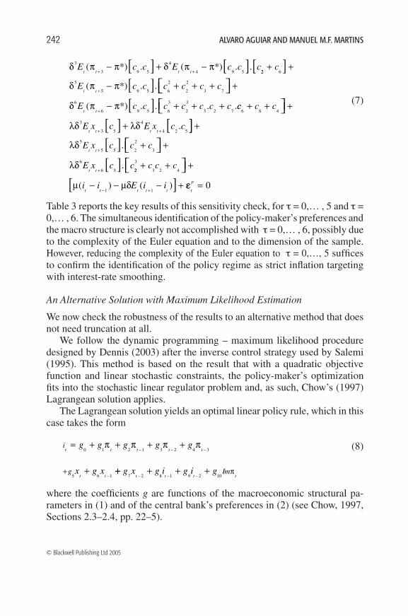
(7)

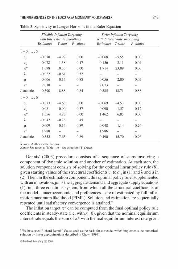
Table 3 reports the key results of this sensitivity check, for τ = 0,… , 5 and τ = 0,… , 6. The simultaneous identification of the policy-maker’s preferences and the macro structure is clearly not accomplished with τ = 0,… , 6, possibly due to the complexity of the Euler equation and to the dimension of the sample. However, reducing the complexity of the Euler equation to τ = 0,…, 5 suffices to confirm the identification of the policy regime as strict inflation targeting with interest-rate smoothing.

An Alternative Solution with Maximum Likelihood Estimation

We now check the robustness of the results to an alternative method that does not need truncation at all.

We follow the dynamic programming – maximum likelihood procedure designed by Dennis (2003) after the inverse control strategy used by Salemi (1995). This method is based on the result that with a quadratic objective function and linear stochastic constraints, the policy-maker’s optimization fits into the stochastic linear regulator problem and, as such, Chow’s (1997) Lagrangean solution applies.

The Lagrangean solution yields an optimal linear policy rule, which in this case takes the form

(8)

where the coefficients g are functions of the macroeconomic structural pa-rameters in (1) and of the central bank’s preferences in (2) (see Chow, 1997, Sections 2.3–2.4, pp. 22–5).

δ π π δ π π3

3 9 5

4

4 9 5E c c E c c c

t t t t( *) . ( *) . .

+ +− + −[ ] [ ] 22 6

5

5 9 5 6

2

2

2

3 7

+ +

− + + +

[ ][ ]

+

c

E c c c c c ct t

δ π π( *) . . [ ]

+

− + + ++

δ π π6

6 9 5 6

3

2

3

3 2 7E c c c c c c c

t t( *) . . . .cc c c

E x c E x c ct t t t

6 8 4

3

3 5

4

4 2 5

+ + +

+

[ ] [+ +

λδ λδ . ]][ ] [ ]

+

+ ++

+

λδ

λδ

5

5 5 2

2

3

6

6 5

E x c c c

E x c c

t t

t t

.

.22

3

3 2 4

1 1

+ + +

− − − +

[ ]− +

c c c

i i E i it t t t t

µ µδ( ) ( ) εεt

p = 0

i

g

t t t t t

t t

g g g g g

x g x

= + + + +

+

− − −

−+

0 1 2 1 3 2 4 3

5 6 1

π π π π

++ + + +− − −

g x g i g i gt t t t

Im7 2 8 1 9 2 10

π

01Ag&Mart221-50*.indd 242 28/4/05 9:45:40 am

243

© Blackwell Publishing Ltd 2005

THE PREFERENCES OF THE EURO AREA MONETARY POLICY-MAKER

9 We have used Richard Dennis’ Gauss code as the basis for our code, which implements the numerical solution by linear approximations described in Chow (1997).

Table 3: Sensitivity to Longer Horizons in the Euler Equation

Flexible Inflation Targeting Strict Inflation Targeting with Interest-rate smoothing with Interest-rate smoothing Estimates T-stats P-values Estimates T-stats P-values

τ = 0, … , 5

c5 –0.078 –4.92 0.00 –0.068 –5.55 0.00

c9 0.078 1.38 0.17 0.156 2.11 0.04

π* 1.698 10.35 0.00 1.714 23.89 0.00

λ –0.022 –0.64 0.52 – – –

μ –0.006 –0.15 0.88 0.056 2.00 0.05

r* 2.018 – – 2.073 – –

J statistic 0.590 18.88 0.84 0.585 18.71 0.88

τ = 0, … , 6

c5 –0.073 –4.63 0.00 –0.069 –4.53 0.00

c9 0.081 0.90 0.37 0.090 1.57 0.12

π* 1.556 4.83 0.00 1.462 6.85 0.00

λ –0.042 –0.76 0.45 – – –

μ 0.009 0.14 0.89 0.048 1.14 0.26

r* 1.988 – – 1.986 – –

J statistic 0.552 17.65 0.89 0.490 15.70 0.96

Source: Authors’ calculations.Notes: See notes to Table 1. τ – see equation (4) above.

Dennis’ (2003) procedure consists of a sequence of steps involving a component of dynamic solution and another of estimation. At each step, the solution component consists of solving for the optimal linear policy rule (8), given starting values of the structural coefficients c

1 to c

10 in (1) and λ and μ in

(2). Then, in the estimation component, this optimal policy rule, supplemented with an innovation, joins the aggregate demand and aggregate supply equations (1), in a three equations system, from which all the structural coefficients of the model – macroeconomic and preferences – are re-estimated by full infor-mation maximum likelihood (FIML). Solution and estimation are sequentially repeated until satisfactory convergence is attained.9

The inflation target π* can be computed from the final optimal policy rule coefficients in steady-state (i.e. with x

t=0), given that the nominal equilibrium

interest rate equals the sum of π* with the real equilibrium interest rate given

01Ag&Mart221-50*.indd 243 28/4/05 9:45:41 am

244

© Blackwell Publishing Ltd 2005

ALVARO AGUIAR AND MANUEL M.F. MARTINS

by c1/(– c

5). In the case of strict inflation targeting, λ is set to zero in the solu-

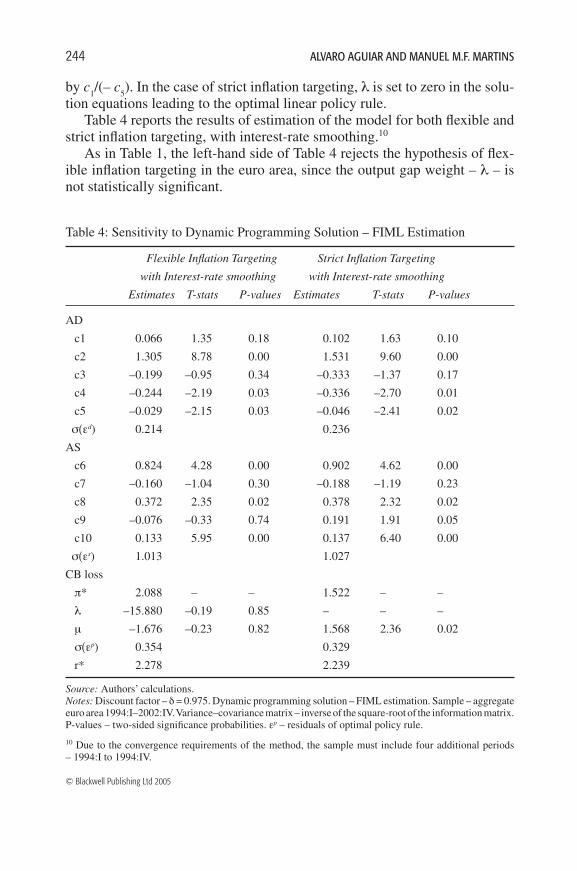
tion equations leading to the optimal linear policy rule.Table 4 reports the results of estimation of the model for both flexible and

strict inflation targeting, with interest-rate smoothing.10 As in Table 1, the left-hand side of Table 4 rejects the hypothesis of flex-

ible inflation targeting in the euro area, since the output gap weight – λ – is not statistically significant.

Table 4: Sensitivity to Dynamic Programming Solution – FIML Estimation

Flexible Inflation Targeting Strict Inflation Targeting

with Interest-rate smoothing with Interest-rate smoothing

Estimates T-stats P-values Estimates T-stats P-values

AD

c1 0.066 1.35 0.18 0.102 1.63 0.10

c2 1.305 8.78 0.00 1.531 9.60 0.00

c3 –0.199 –0.95 0.34 –0.333 –1.37 0.17

c4 –0.244 –2.19 0.03 –0.336 –2.70 0.01

c5 –0.029 –2.15 0.03 –0.046 –2.41 0.02

σ(εd) 0.214 0.236

AS

c6 0.824 4.28 0.00 0.902 4.62 0.00

c7 –0.160 –1.04 0.30 –0.188 –1.19 0.23

c8 0.372 2.35 0.02 0.378 2.32 0.02

c9 –0.076 –0.33 0.74 0.191 1.91 0.05

c10 0.133 5.95 0.00 0.137 6.40 0.00

σ(εs) 1.013 1.027

CB loss

π* 2.088 – – 1.522 – –

λ –15.880 –0.19 0.85 – – –

μ –1.676 –0.23 0.82 1.568 2.36 0.02

σ(εp) 0.354 0.329

r* 2.278 2.239

Source: Authors’ calculations. Notes: Discount factor – δ = 0.975. Dynamic programming solution – FIML estimation. Sample – aggregate euro area 1994:I–2002:IV. Variance–covariance matrix – inverse of the square-root of the information matrix. P-values – two-sided significance probabilities. εp – residuals of optimal policy rule.

10 Due to the convergence requirements of the method, the sample must include four additional periods – 1994:I to 1994:IV.

01Ag&Mart221-50*.indd 244 28/4/05 9:45:41 am

245

© Blackwell Publishing Ltd 2005

THE PREFERENCES OF THE EURO AREA MONETARY POLICY-MAKER

The right-hand side of Table 4 confirms our previous results that a central bank loss function of strict inflation targeting with interest-rate smoothing (μ becomes statistically significant) fits well the aggregate euro area monetary policy-making. Furthermore, the estimates of the inflation target (π* = 1.5 per cent) and the real equilibrium interest rate (r* = 2.2 per cent) are quite close to those reported in Table 1. In contrast, the estimate of the relative weight of interest-rate smoothing – μ – differs substantially from that in Table 1. This discrepancy may be caused by differences in the solution procedures – such as the truncation – or in the estimation methods. Its explanation, however, is beyond the scope of this article (see Dennis, 2003, and Söderlind et al., 2005, for some discussion of the US case, in which the discrepancy is even larger than the one we document for the euro area).

Inflation Targeting without Interest-Rate Smoothing

So far, the analysis points strongly to the presence of interest-rate smooth-ing in the policy-makers’ loss function. We perform now a final check on the identification of the monetary policy regime by constraining the smoothing coefficient, μ, to zero.

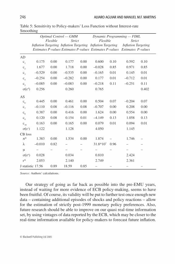
Unsurprisingly – due to the significance of interest-rate smoothing – the performance of the model is weakened, as depicted in Table 5, where the thor-ough results of the check are reported.11 It is clear, however, that the rejection of flexible inflation targeting in favour of strict inflation targeting does not depend on the presence of interest-rate smoothing.

Concluding Remarks

This article estimated – in the context of a simple dynamic backward-looking macroeconomic structure – the aggregate monetary policy preferences in the euro area in the form of a loss function with strict inflation targeting at 1.6 per cent and interest-rate smoothing.

Through a combined analysis of facts, data and literature on European inte-gration, we have identified 1995 as the start date of a euro area notional policy regime, in the sense that it is reasonable to consider the group of central banks of the current EMU as if they were already a single monetary authority. In this view, the common policy preferences have a role in explaining the fall in the volatility of both the output gap and inflation since the mid-1990s.

11 The right-hand side of the table shows that setting µ to zero leads to unreasonable estimates and a poor performance of the model. This is because maximum likelihood estimation of mis-specified models may result in very odd results – by its very nature, FIML tries to find values for the parameters that make the largest equation error as small as possible.

01Ag&Mart221-50*.indd 245 28/4/05 9:45:42 am

246

© Blackwell Publishing Ltd 2005

ALVARO AGUIAR AND MANUEL M.F. MARTINS

Our strategy of going as far back as possible into the pre-EMU years, instead of waiting for more evidence of ECB policy-making, seems to have been fruitful. Of course, its validity will be put to further test once enough new data – containing additional episodes of shocks and policy reactions – allow for the estimation of strictly post-1999 monetary policy preferences. Also, future research should be able to improve on our quasi real-time information set, by using vintages of data reported by the ECB, which may be closer to the real-time information available for policy-makers to forecast future inflation.

Table 5: Sensitivity to Policy-makers’ Loss Function without Interest-rate Smoothing Optimal Control — GMM Dynamic Programming — FIML Flexible Strict Flexible Strict Inflation Targeting Inflation Targeting Inflation Targeting Inflation Targeting Estimates P-values Estimates P-values Estimates P-values Estimates P-values

AD c

1 0.175 0.00 0.177 0.00 0.600 0.10 0.592 0.10

c2 1.677 0.00 1.718 0.00 –0.028 0.85 0.971 0.85

c3 –0.529 0.00 –0.535 0.00 –0.165 0.01 0.145 0.01

c4 –0.254 0.00 –0.282 0.00 0.177 0.01 –0.712 0.01

c5 –0.085 0.00 –0.083 0.00 –0.218 0.11 –0.251 0.11

σ(εd) 0.256 0.260 0.765 0.402

AS c

6 0.445 0.00 0.461 0.00 0.504 0.07 –0.204 0.07

c7 –0.110 0.08 –0.116 0.08 –0.707 0.00 0.208 0.00

c8 0.387 0.00 0.416 0.00 1.624 0.00 0.554 0.00

c9 0.120 0.08 0.154 0.01 –4.149 0.13 1.058 0.13

c10

0.163 0.00 0.165 0.00 0.079 0.01 0.094 0.01

σ(εs) 1.122 1.128 4.050 1.145

CB loss π* 1.383 0.00 1.534 0.00 1.874 – 1.746 –

λ –0.010 0.82 – – 31.8*107 0.96 – –

μ – – – – – – – –

σ(εp) 0.028 0.034 0.810 2.424

r* 2.053 2.140 2.749 2.361

J statistic 17.56 0.89 18.59 0.85 – – – –

Source: Authors’ calculations.

01Ag&Mart221-50*.indd 246 28/4/05 9:45:42 am

247

© Blackwell Publishing Ltd 2005

THE PREFERENCES OF THE EURO AREA MONETARY POLICY-MAKER

Correspondence:Manuel M. F. MartinsCempre, Faculdade de Economia, Universidade do PortoRua Roberto Frias 4200-464 Porto, PortugalTel:+351 225571100 Fax: +351 225505050email: [email protected]

References

Agresti, A.-M. and Mojon, B. (2001) ‘Some Stylised Facts on the Euro Area Business Cycle’. ECB Working Paper No. 95, December.

Aguiar, A. and Martins, M.M.F (2004) ‘Testing the Significance and the Non-linearity of the Phillips Trade-off in the Euro Area’. Empirical Economics, forthcoming.

Aksoy, Y., De Grauwe, P. and Dewachter, H. (2002) ‘Do Asymmetries Matter for European Monetary Policy?’. European Economic Review, Vol. 46, No. 3, pp. 443–69.

Andrews, D.W.K. (1993) ‘Tests for Parameter Instability and Structural Change with Unknown Change Point’. Econometrica, Vol. 61, No. 4, pp. 821–56.

Angeloni, I., Kashyap, A., Mojon, B. and Terlizzese, D. (2003) ‘Monetary Transmis-sion in the Euro Area: Where do We Stand?’. In Angeloni, I., Kashyap, A. and Mojon, B. (eds) Monetary Policy Transmission in the Euro Area (Cambridge/New York/Melbourne: Cambridge University Press).

Artis, M., Krolzig, H.-M. and Toro, J. (2004) ‘The European Business Cycle’. Oxford Economic Papers, Vol. 56, No. 1, pp. 1–44.

Artis, M., Marcellino, M. and Proiett, T. (2005) ‘Dating the Euro Area Business Cycle’. In Reichlin, L. (ed.) The Euro Area Business Cycle: Stylized Facts and Measurement Issues (London: Centre for Economic Policy Research) forthcoming.

Begg, D., Canova, F., De Grauwe, P., Fatás, A. and Lane, P.R. (2002) Surviving the Slowdown, Monitoring the European Central Bank 4 (London: Centre for Economic Policy Research).

Chow, G. (1997) Dynamic Economics – Optimization by the Lagrange Method (New York/Oxford: Oxford University Press).

Clarida, R. and Gertler, M. (1997) ‘How the Bundesbank Conducts Monetary Policy’. In Romer, C. and Romer, D. (eds) Reducing Inflation – Motivation and Strategy, NBER Studies in Business Cycles, 30 (Chicago: University of Chicago Press).

Clarida, R., Galí, J. and Gertler, M. (1998) ‘Monetary Policy Rules in Practice: Some In-ternational Evidence’. European Economic Review, Vol. 42, No. 6, pp. 1033–67.

Coenen, G., Levin, A. and Wieland, V. (2005) ‘Data Uncertainty and the Role of Money as an Information Variable for Monetary Policy’. European Economic Review, Vol. 49, No. 4, pp. 975–1006.

Dennis, R. (2003) ‘The Policy Preferences of the US Federal Reserve’. Federal Re-serve Bank of San Francisco Working Paper No. 2001-08, revised edn, Journal of Applied Econometrics, forthcoming.

01Ag&Mart221-50*.indd 247 28/4/05 9:45:43 am

248

© Blackwell Publishing Ltd 2005

ALVARO AGUIAR AND MANUEL M.F. MARTINS

English, W.B., Nelson, W.R. and Sack, B.P. (2003) ‘Interpreting the Significance of the Lagged Interest Rate in Estimated Monetary Policy Rules’. Contributions to Macroeconomics, Vol. 3, No. 1.

European Central Bank (2002) ‘Protocol on the Statute of the European System of Central Banks and of the European Central Bank’. In ECB Compendium 2002 – Col-lection of Legal Instruments June 1998 – December 2001 (in English), Frankfurt, Available at «http:www.ecb.int/pub/pdf/legalcomp02en.pdf».

European Central Bank Monthly Bulletin (2000–03) Various issues. Available at «http:www.ecb.int/pub».

Fagan, G., Jerome H.J. and Mestre, R. (2001) ‘An Area-Wide Model (AWM) for the Euro Area’. European Central Bank Working Paper No. 42.

Favero, C.A. (2001) ‘Does Macroeconomics Help Understand the Term Structure of Interest Rates?’. Università Bocconi IGIER Working Paper, No. 195.

Favero, C.A. and Rovelli, R. (2003) ‘Macroeconomic Stability and the Preferences of the FED. A Formal Analysis, 1961–98’. Journal of Money, Credit and Banking, Vol. 35 No. 4, pp. 545–56.

Florens, C., Jondeau, E. and Le Bihan, H. (2001) ‘Assessing GMM Estimates of the Federal Reserve Reaction Function’. Banque de France Notes d’Études et de Recherche No. 83.

Fuhrer, J. (1997) ‘Inflation–Output Variance Trade-Offs and Optimal Monetary Policy’. Journal of Money, Credit and Banking, Vol. 29, No. 2, pp. 214–34.

Gaspar, V. and Issing, O. (2002) ‘Exchange Rates and Monetary Policy’. Australian Economic Papers, Vol. 41, No. 4, pp. 342–65.

Goodhart, C. (1998) ‘Central Bankers and Uncertainty’. London School of Economics, Financial Markets Group Special Paper Series No. 106.

Goodhart, C. (2001) ‘Monetary Transmission Lags and the Formulation of the Policy Decision on Interest Rates’. Federal Reserve Bank of St. Louis Review, Vol. 83, No. 4, pp. 165–81.

Hansen, B.E. (2001) ‘The New Econometrics of Structural Change: Dating Breaks in U.S. Labor Productivity’. Journal of Economic Perspectives, Vol. 15, No. 4, pp. 117–28.

Hansen, L.P., Heaton, J. and Yaron, A. (1996) ‘Finite Sample Properties of Alternative GMM Estimators’. Journal of Business and Economic Statistics, Vol. 14, No. 3, pp. 262–81.

Harvey, A. (1989) Forecasting, Structural Time Series Models and the Kalman Filter (Cambridge: Cambridge University Press).

IMF (2001) World Economic Outlook – The Information Technology Revolution (Washington, DC: IMF).

Luginbuhl, R. and Koopman, S.J. (2004) ‘Convergence in European GDP Series: A Multivariate Common Converging Trend-Cycle Decomposition’. Journal of Ap-plied Econometrics, Vol. 19, No. 5, pp. 611–36.

McCallum, B. (1997) ‘Crucial Issues Concerning Central Bank Independence’. Journal of Monetary Economics, Vol. 39, No. 1, pp. 99–112.

McCallum, B. (2001a) ‘Should Monetary Policy Respond Strongly to Output Gaps?’. American Economic Review, Vol. 91, No. 2 pp. 258–62.

01Ag&Mart221-50*.indd 248 28/4/05 9:45:43 am

249

© Blackwell Publishing Ltd 2005

THE PREFERENCES OF THE EURO AREA MONETARY POLICY-MAKER

McCallum, B. (2001b) ‘Monetary Policy Analysis in Models without Money’. Federal Reserve Bank of St. Louis Review, Vol. 83, No. 4, pp. 145–60.

Mihov, I. (2001) ‘One Monetary Policy in EMU’. Economic Policy, Vol. 16, No. 33, pp. 369–406.

Nelson, E. and Nikolov, K. (2003) ‘UK Inflation in the 1970s and 1980s: The Role of Output Gap Mismeasurement’. Journal of Economics and Business, Vol. 55, No. 4, pp. 353–70.

Orphanides, A. (2001) ‘Monetary Policy Rules Based on Real-Time Data’. American Economic Review, Vol. 91, No. 4, pp. 964–85.

Orphanides, A. (2002) ‘Monetary Policy Rules and the Great Inflation’. American Economic Review, Vol. 92, No. 2, pp. 115–20.

Orphanides, A. (2004) ‘Monetary Policy Rules, Macroeconomic Stability and Infla-tion: A View From the Trenches’. Journal of Money, Credit and Banking, Vol. 36, No. 2, pp. 151–75.

Peersman, G. and Smets, F. (1999) ‘The Taylor Rule: A Useful Monetary Policy Bench-mark for the Euro Area?’. International Finance, Vol. 2, No. 1, pp. 85–116.

Peersman, G. and Smets, F. (2003) ‘The Monetary Transmission Mechanism in the Euro Area: More Evidence from VAR Analysis’. In Angeloni, A., Kashyap, A. and Mojon, B. (eds) Monetary Policy Transmission in the Euro Area (Cambridge/New York/Melbourne: Cambridge University Press).

Perez, S.J. (2001) ‘Looking Back at Forward-Looking Monetary Policy’. Journal of Economics and Business, Vol. 53, No. 5, pp. 509–21.

Rudebusch, G. (2002) ‘Term Structure Evidence on Interest-rate smoothing and Monetary Policy Inertia’. Journal of Monetary Economics, Vol. 49, No. 6, pp. 1161–87.

Rudebusch, G. and Svensson, L. (1999) ‘Policy Rules for Inflation Targeting’. In Taylor, J. (ed.) Monetary Policy Rules, National Bureau of Economic Research Conference Report (Chicago: University of Chicago Press).

Rudebusch, G. and Svensson, L. (2002) ‘Eurosystem Monetary Targeting: Lessons from U.S. Data’. European Economic Review, Vol. 46, No. 3, pp. 417–42.

Sack, B. (2000) ‘Does the FED Act Gradually? A VAR Analysis’. Journal of Monetary Economics, Vol. 46, No. 1, pp. 229–56.

Sack, B. and Wieland, V. (2000) ‘Interest-Rate Smoothing and Optimal Monetary Policy: A Review of Recent Empirical Evidence’. Journal of Economics and Busi-ness, Vol. 52, No. 1/2, pp. 205–28.

Salemi, M.K. (1995) ‘Revealed Preferences of the Federal Reserve: Using Inverse-Control Theory to Interpret the Policy Equation of a Vector Autoregression’. Journal of Business and Economic Statistics, Vol. 13, No. 4, pp. 419–33.

Smets, F. (2003) ‘Maintaining Price Stability: How Long is Medium Term?’. Journal of Monetary Economics, Vol. 50, No. 6, pp. 1293–309.

Smets, F. and Wouters, R. (2004) ‘Comparing Shocks and Frictions in US and Euro Area Business Cycles: A Bayesian DSGE Approach’. Centre for Economic Policy Research Discussion Paper No. 4750.

Söderlind, P., Söderström, U. and Vredin, A. (2005) ‘New-Keynesian Models and Monetary Policy: A Reexamination of the Stylized Facts’. Scandinavian Journal of Economics, forthcoming.

01Ag&Mart221-50*.indd 249 28/4/05 9:45:44 am

250

© Blackwell Publishing Ltd 2005

ALVARO AGUIAR AND MANUEL M.F. MARTINS

Stock, J. and Watson, M. (1998) ‘Median Unbiased Estimation of a Coefficient Vari-ance in a Time-Varying Parameter Model’. Journal of the American Statistical Association, Vol. 93, No. 441, pp. 349–58.

Svensson, L.E.O. (2003) ‘The Inflation Forecast and the Loss Function’. In Mizen, P. (ed.) Central Banking, Monetary Theory and Practice: Essays in Honour of Charles Goodhart, Vol. I (Cheltenham: Edward Elgar).

Taylor, J.B. (1979) ‘Estimation and Control of a Macroeconomic Model with Rational Expectations’. Econometrica, Vol. 47, No. 5, pp. 1267–86.

Taylor, J.B. (1994) ‘The Inflation–Output Variability Trade-Off Revisited’. In Fuhrer, J.C. (ed.) Goals, Guidelines, and Constraints Facing Monetary Policy-makers, Conference Series No. 38 (Federal Reserve Bank of Boston).

Taylor, J.B. (1999) ‘The Robustness and Efficiency of Monetary Policy Rules as Guidelines for Interest Rate Setting by the European Central Bank’. Journal of Monetary Economics, Vol. 43, No. 3, pp. 655–79.

01Ag&Mart221-50*.indd 250 28/4/05 9:45:44 am