The Potential of Low-Cost Tin-Oxide Sensors ... - MDPI

atmosphere

Article

The Potential of Low-Cost Tin-Oxide Sensors Combined withMachine Learning for Estimating Atmospheric CH4 Variationsaround Background Concentration

Rodrigo Rivera Martinez 1,* , Diego Santaren 1, Olivier Laurent 1 , Ford Cropley 1, Cécile Mallet 2 ,Michel Ramonet 1 , Christopher Caldow 1 , Leonard Rivier 1, Gregoire Broquet 1, Caroline Bouchet 3,Catherine Juery 4 and Philippe Ciais 1

Citation: Rivera Martinez, R.;

Santaren, D.; Laurent, O.; Cropley, F.;

Mallet, C.; Ramonet, M.; Caldow, C.;

Rivier, L.; Broquet, G.; Bouchet, C.;

et al. The Potential of Low-Cost

Tin-Oxide Sensors Combined with

Machine Learning for Estimating

Atmospheric CH4 Variations around

Background Concentration.

Atmosphere 2021, 12, 107.

https://doi.org/10.3390/

atmos12010107

Received: 18 November 2020

Accepted: 11 January 2021

Published: 13 January 2021

Publisher’s Note: MDPI stays neu-

tral with regard to jurisdictional clai-

ms in published maps and institutio-

nal affiliations.

Copyright: © 2021 by the authors. Li-

censee MDPI, Basel, Switzerland.

This article is an open access article

distributed under the terms and con-

ditions of the Creative Commons At-

tribution (CC BY) license (https://

creativecommons.org/licenses/by/

4.0/).

1 Laboratoire des Sciences du Climat et de l’Environnement (LSCE), LSCE/IPSL, CEA-CNRS-UVSQ, UniversitéParis-Saclay, 91191 Gif-sur-Yvette, France; [email protected] (D.S.); [email protected] (O.L.);[email protected] (F.C.); [email protected] (M.R.); [email protected] (C.C.);[email protected] (L.R.); [email protected] (G.B.); [email protected] (P.C.)

2 Laboratoire Atmosphères Milieux, Observations Spatiales (LATMOS), UMR8190, CNRS/INSU, IPSL,Universite de Versailles Saint-Quentin-en-Yvelines (UVSQ), Quartier des Garennes, 11 Boulevard d’Alembert,78280 Guyancourt, France; [email protected]

3 SUEZ, Smart & Environmental Solutions, Tour CB21, 16 Place de l’Iris, 92040 La Defense, France;[email protected]

4 Total Raffinage Chimie, Laboratoire Qualite de l’Air, 69360 Solaize, France; [email protected]* Correspondence: [email protected]

Abstract: Continued developments in instrumentation and modeling have driven progress in moni-toring methane (CH4) emissions at a range of spatial scales. The sites that emit CH4 such as landfills,oil and gas extraction or storage infrastructure, intensive livestock farms account for a large shareof global emissions, and need to be monitored on a continuous basis to verify the effectiveness ofreductions policies. Low cost sensors are valuable to monitor methane (CH4) around such facilitiesbecause they can be deployed in a large number to sample atmospheric plumes and retrieve emissionrates using dispersion models. Here we present two tests of three different versions of Figaro®

TGS tin-oxide sensors for estimating CH4 concentrations variations, at levels similar to currentatmospheric values, with a sought accuracy of 0.1 to 0.2 ppm. In the first test, we characterize thevariation of the resistance of the tin-oxide semi-conducting sensors to controlled levels of CH4, H2Oand CO in the laboratory, to analyze cross-sensitivities. In the second test, we reconstruct observedCH4 variations in a room, that ranged from 1.9 and 2.4 ppm during a three month experiment fromobserved time series of resistances and other variables. To do so, a machine learning model is trainedagainst true CH4 recorded by a high precision instrument. The machine-learning model using 30% ofthe data for training reconstructs CH4 within the target accuracy of 0.1 ppm only if training variablesare representative of conditions during the testing period. The model-derived sensitivities of the sen-sors resistance to H2O compared to CH4 are larger than those observed under controlled conditions,which deserves further characterization of all the factors influencing the resistance of the sensors.

Keywords: low-cost sensors; artificial neural networks; methane; calibration

1. Introduction

Anthropogenic CH4 emissions comprise 30% of the global source of this greenhousegas, and are from various economic sectors [1]. Oil, gas and coal sector sources are localizedin space, going from point scale (e.g., a single well, a compressor) to area sources (e.g.,a refinery, a gas extraction field). The waste sector has area sources for waste-watertreatment plants and landfills, although within a site there can be leaky equipment formingpoint sources.

Atmosphere 2021, 12, 107. https://doi.org/10.3390/atmos12010107 https://www.mdpi.com/journal/atmosphere

Atmosphere 2021, 12, 107 2 of 22

Numerous campaigns estimated emissions from point and area sources using atmo-spheric measurements by deploying local dense networks of CH4 instruments at fixedpoints and using mobile ground-based platforms and aircraft [2–4]. The signal from asource in terms of CH4 concentration at a nearby atmospheric measurement location de-pends on the magnitude of this source, on the wind speed, on the atmospheric turbulenceand on the sampling distance. An excess of CH4 mixing ratio going from a few tenth partsper billion (ppb) [5,6] up to several parts per million (ppm) [7] is typically recorded at adownwind distance from the source.

Research class CH4 analyzers such as Cavity Ring Down Spectrometers (CRDS) usedfor background air monitoring have a precision higher than 1 ppb [8,9] but they are expen-sive. Such precision is needed to monitor the small CH4 gradients between backgroundstations, on the order of 10 to 50 ppb, that are used as an input of atmospheric inversionmodels to diagnose large-scale emissions [10]. The deployment of multiple CRDS instru-ments in the vicinity of an industrial site for detecting and/or estimating its emissions ishowever a too costly option on a routine basis, especially when needing a very dense net-work to ensure precise location and quantification of a fugitive source. This has promptedresearch to develop low-cost sensors with a precision sufficient to characterize the signal ofatmospheric plumes from industrial sites. From typical plume signals that are on the orderof more than a ppm, a precision of 0.1 to 0.2 ppm on instantaneous measurements can bedeemed to be sufficient for a low cost CH4 sensors. Low cost sensors are more likely to driftwith time than CRDS analyzers, but the atmospheric signal used to quantify the emissionof an industrial site is the near instantaneous difference between upwind and downwindconcentrations [7,11]. Therefore, constraining the drift of upwind and downwind sensorsduring a few hours to be less than 0.1 to 0.2 ppm would still be sufficient for monitoringCH4 emissions from an industrial site.

Here, we formulate a target precision requirement of 0.1 to 0.2 ppm over a time scaleof one hour for CH4 low cost sensors to be deployed on dense networks around an emittingsource. This requirement is suitable for detecting variations of CH4 in background air,which are on the order of 0.1 ppm on an hourly time scale, and characterize CH4 conditionsupwind from an emitting source. We tested for this requirement solid-state tin-oxide (SnO2)sensors models TGS 2600, TGS 2611-C00 and TGS 2611-E00 manufactured by Figaro®. Weperformed measurements of room air where CH4 concentration varies from day to dayby up to 0.5 ppm above a background value of 1950 ppb. The principle of those sensorsis to measure changes in the tin-oxide resistance affected by electron donors in the air towhich the tin-oxide is exposed. These sensors are cheap, with a unit cost of about 3 € to25 € per sensor and they were shown to be sensitive to low CH4 concentrations, thus beingpotentially suitable for emissions monitoring with a good characterization of backgroundvariations and plume amplitudes even for modest sources [3]. On the other hand, low costsensors are known to drift with time, to be sensitive to other reduced species than CH4 andto factors such as water vapor, pressure and temperature [12]. Therefore, cross sensitivitiesto these other species must be characterized in order to understand how they impact theretrieval of CH4 from measured variations of resistance.

The first research question addressed in this study is to characterize the cross sensitiv-ities of Figaro® resistances to CH4 versus other factors known to influence the tin-oxideresistance: carbon monoxide (CO), water vapor, pressure and temperature [13]. To addressthis question, we characterized in a laboratory facility under controlled conditions theresistances of six Figaro® sensors for a range of CH4, CO, temperature and H2O, andexamined covariance between their sensitivities, in a first step to diagnose cross-sensitivityeffects from non-CH4 related variables.

The second research question is to test whether measurements of low-cost sensorsresistance combined with other cross-sensitivity variables allow for the reconstruction ofCH4 concentration and its variability to meet our precision requirement of 0.1 to 0.2 ppm,here in the case of CH4 variations around background values of up to 0.5 ppm. To addressthis second question, we analyzed time series of Figaro® resistances continuously recorded

Atmosphere 2021, 12, 107 3 of 22

by six Figaro® sensors and CH4 measured with a high-precision CRDS analyzer for room airCH4 variations, during a period of 47 days. This study is the first step to assess the potentialof Figaro® sensors for measuring CH4 concentrations close to current atmospheric levels;with small co-variations of water vapor and of a limited number of cross-sensitive species.On previous studies [12] and on initial tests showing that there is a non-linear relationbetween CH4, resistances and other variables affecting resistances such as temperatureand H2O mole fraction, we chose to construct and apply a machine learning model toreconstruct the true CH4 concentration from the CRDS by using as predictors the resistancesof the Figaro® sensors, as well as H2O mixing ratio, carbon monoxide, temperature andpressure recorded by other sensors. The model is trained to optimally reconstruct the trueCH4 signal during a given period, and its results are evaluated against an independentsubset of the data. The results are systematically evaluated varying the training and testperiods, the number of ambient variables, and the addition of more than one type ofFigaro® sensor resistance to reconstruct the true CH4 time series.

2. Experimental Set-Up2.1. Measurement of Low-Cost Sensors Sensitivities to CH4, CO and H2O

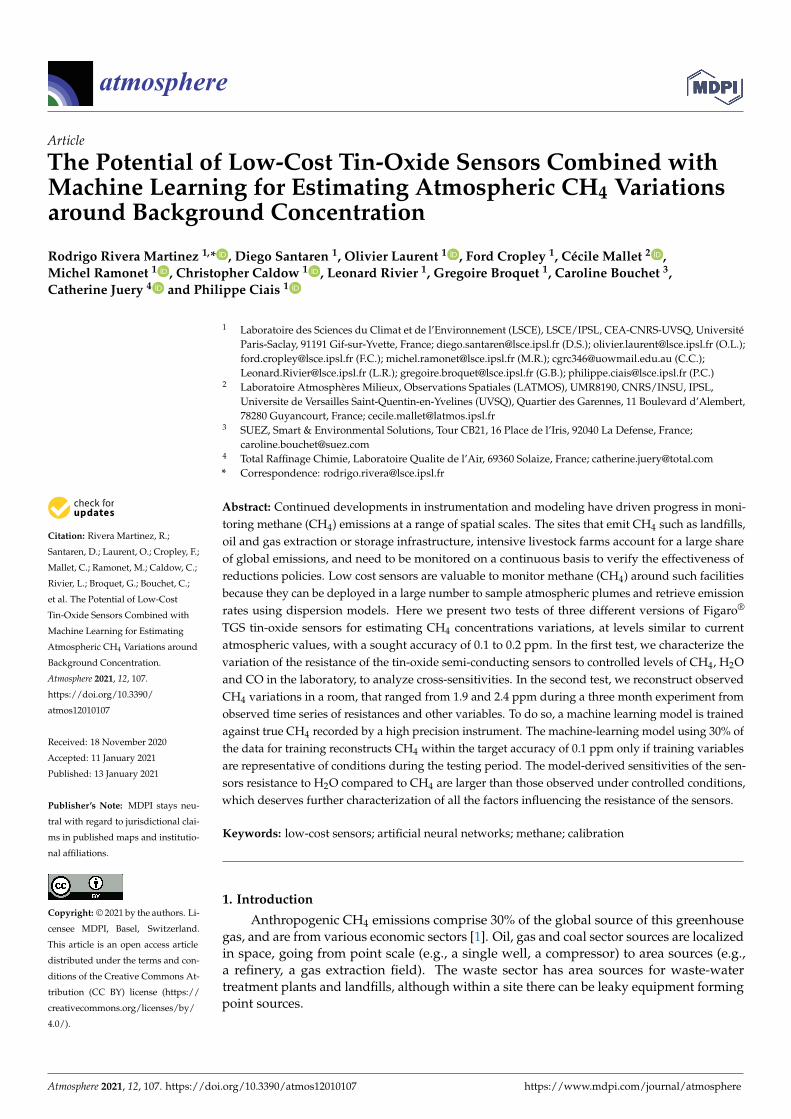
The cross sensitivities of the resistance of Figaro® sensors types TGS 2600, TGS 2611-C00, and TGS 2611-E00 were measured in the laboratory (measurements conducted atLSCE, Saclay, France). The sensors were incorporated into a low-cost sensor logger thatfeatured a Raspberry Pi 3B+ single-board computer and Raspbian operating system, usingbespoke software (coded in Python). Figaro resistances for types TGS 2600, TGS 2611-C00and TGS 2611-E00 were measured as voltages using a voltage divider [14,15] with precisionresistor (5 kΩ, tolerance, temp coeff), and measured as single-ended voltages using anA/D board (ADCPiPlus, ABElectronics) with 17-bit resolution across the 5.06 V range. Airtemperature and relative humidity were measured using a Sensirion SHT75 digital sensorwhich has an accuracy of ±0.3 C and ±1.8%RH respectively and a repeatability of ±0.1 Cand ±0.1 %RH respectively. Air pressure was measured using a digital Bosch BMP180pressure sensor (Adafruit, BMP180 breakout module), which has an accuracy of ±0.12%across the range 950-1050 hPa. All sensors were mounted in a 120 mL stainless steel/glasssealed chamber (EIF 3S1NRGL), which provided a gas inlet and outlet and an air-tight portfor the sensor cable (see Figure 1a). All measurements were made at 0.5 Hz and stored onthe Raspberry Pi’s SD card.

To assess the sensitivities of the sensor resistances to CH4 and H2O, we used air fromtwo high pressure dry air cylinders, with a high CH4 mole fraction of 8.999 ppm CH4and 0.08 ppm CO, and a low CH4 mole fraction of 1.900 ppm CH4 and 0.11 ppm CO,respectively. Air from the two cylinders was mixed using two mass flow controllers (seeFigure 1b) to create six levels of CH4 of 1.9, 2.985, 4.04, 6.17, 7.58 and 8.985 ppm in dry air.This range covers CH4 mole fractions recorded in the atmosphere from background sitesup to typical excess found in plumes from industrial sites [16]. The air with different CH4concentration was humidified by a dew-point generator (Licor, LI-610) in order to get fourH2O mixing ratios of 0.65, 1, 1.5 and 2.5% at stable atmospheric pressure and temperature.The experiment set up is illustrated in Figure 1b.

In the experiment, the dew point generator was set to one of the four H2O mixingratios. At each change of H2O mixing ratio, the Figaro® reading was given 40 or moreminutes to stabilize at the lowest CH4 level, before CH4 was increased in steps at 20 minintervals. Only the last 5 min’ data of each step was used. Data from the sensors and thePicarro CRDS were merged and converted to one-minute medians.

The Figaro® sensors’ sensitivity to CO and H2O was measured in a similar manner,using a single high pressure dry air cylinder containing 1.5 ppm CO and 2 ppm CH4. Thesample line was split into two branches, one equipped with Sofnocat 514, a hydrophobicCO oxidizing agent, to remove CO without changing the humidity. The air from the twolines was combined in different ratios thanks to dedicated mass flow controllers in orderto produce CO mole fractions of 0, 0.07, 0.14, 0.29, 0.57, 0.87, 1.17 and 1.50 ppm, at H2O

Atmosphere 2021, 12, 107 4 of 22

mixing ratios of 0, 1.0 and 2.3% thanks to a dew point generator (Licor, LI-610) operated atconstant temperature and pressure. The experimental configuration is shown in Figure 1c.The logging equipment and sampling procedure were the same as for the first experiment.

In this experiment, a Picarro G2401 CRDS was used as a reference high-precisioninstrument for CH4, CO2, CO and H2O mole fraction. The CH4 precision of a PicarroCRDS analyzer in dry air is below 1 ppb [6,17] at instrument data acquisition rate (0.3 Hz)within the atmospheric range. CRDS calibration drift over time is usually better than 1 ppbCH4 per month [6].

Figure 1. (a) Picture showing the sealed chamber with six Figaro® sensors of different types, andtemperature and pressure sensors. (b) Scheme of the CH4 and H2O cross-sensitivity measurementset up. (c) Scheme of the CO and H2O cross-sensitivity measurement set up.

2.2. Measurements of Room Air with Low Cost Sensors and CRDS

The resistances of six Figaro® sensors exposed to CH4 variability in indoor air weremonitored during 47 days (from 27 April to 12 June of 2018) in an air-conditioned room,with three versions of Figaro® sensors: TGS 2600, TGS 2611-C00 and TGS 2611-E00. Detailsof the data acquisition are as described in the previous section. Reference data was againprovided by a Picarro G2401 gas analyzer. Air temperature and relative humidity was mea-sured using a DHT22 digital sensor (Aosong Electronics) which has an accuracy of ±0.5 Cand ±0.5% RH respectively. The sensors were installed in a semi-open enclosure fromwhich the Picarro CRDS took its intake, thus sampling the same air that the Figaro®sensors.

3. Modeling CH4 from Figaro Resistances and Other Predictors

Low-cost sensors, generally, present a non-linear dependency on environmental vari-ables causing cross-sensitivities [3]. There is no mathematical model of the relationshipbetween the resistances and CH4, given the dependency of resistances on other envi-ronmental variables (CO, H2O, pressure and temperature). The analytical problem thusremains nonlinear and multi-dimensional. Therefore, an Artificial Neural Network model(ANN) was chosen to reconstruct CH4 from observed time series of resistances, CO, H2O,pressure and temperature. We chose a Multi Layer Perceptron (MLP) which is a classicalsupervised-based algorithm [18]. MLP models are generally considered to be the referenceamong machine learning methods because several theoretical results prove their abilityas a universal approximator [19,20], capable of learning from examples. For our prob-lem, the advantages of a machine learning model such as MLP are the following: (i) itdoes not require any prior knowledge about I/O dependencies, (ii) it is able to constructarbitrary functions from noisy data [21], it makes no assumption on the distribution ofdata [22], and (iii) could produce reasonable outputs from entries that are not present inthe learning set, i.e., generalization [23]. Over the past decade, deep networks such as MLP

Atmosphere 2021, 12, 107 5 of 22

have demonstrated superior performance over a wide variety of tasks, including functionapproximation. Recently, MLP have been proven to be more efficient than inverse linearmethods in reconstructing the signals of trace gas species from low-cost sensors [24].

In a MLP model, unknown parameters (i.e., architecture and connection weights)are adjusted in order to obtain the best match between a dataset of model inputs (Figaroresistances, H2O, CO, Temperature and Pressure) and corresponding outputs (Figaro CH4).The connection weights are adjusted by using iterative learning processes such as thebackpropagation [18] or several algorithms that have been developed in order to achieve agood learning of the model (i.e., Stochastic gradient descent, Adam, etc., [25]). In our study,we chose to use a quasi-Newton method, the Broyden-Fletcher-Goldfarb-Shanno (BFGS)algorithm, which provide the optimal MLP weights in a limited number of iterations (300)due to its relatively fast convergence [23]. For our study, the architecture of the MLPproducing the best results was found to be a four-layer network with 5 units in the inputlayer, 14 and 19 units with tanh activation function in the hidden layer and 1 unit with alinear activation function in the output layer. All models were constructed using the libraryscikit-learn [26] on python 3.6.

The generalization error, also called test error, is the expected value of the errorproduced by new inputs [27]. This error is obtained from the performance of the MLPto match an independent test dataset. A central challenge of function approximation byMLPs is the risk of underfitting and overfitting [27]. Underfitting is referred to a hightraining error when, because of an inconvenient architecture or because of training inputsthat are not explanatory enough for example, the MLP does not manage to efficiently fitthe training data set. In our case, the risk of underfitting is mitigated by using a sufficientlycomplex model. Overfitting happens when the MLP learns features from the training dataset, e.g., noise or biases, that are not relevant and do not generalize well to a different dataset. To reduce the risk of overfitting we used the weight decay regularizer or L2 Normthat drives excess weights (weights of the network that does have little or no influencein the model) to values close to zero [23]. We use also an early stopping technique thatconstantly monitors the error produced by the model with respect to an independentvalidation data set (validation error) during the learning process. When the validation errorstarts increasing, the training process is stopped in order to moderate the generalizationerror [21,27]. The best MLP model was selected as the one producing the lowest validationerror from the results of many tests in which the number of neurons of the hidden layerwere varied (see Section 4.4).

4. Results4.1. Sensitivities of Low-Cost Sensors

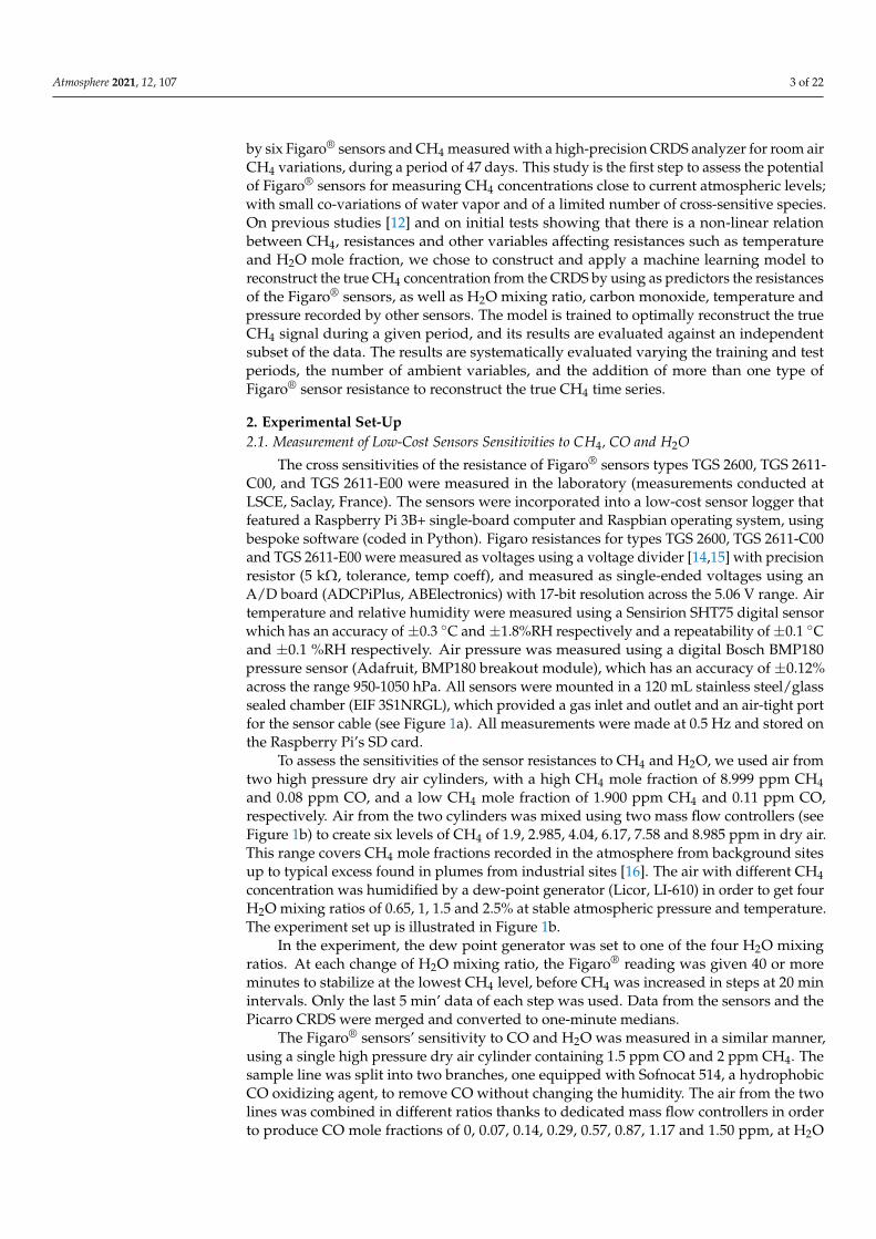
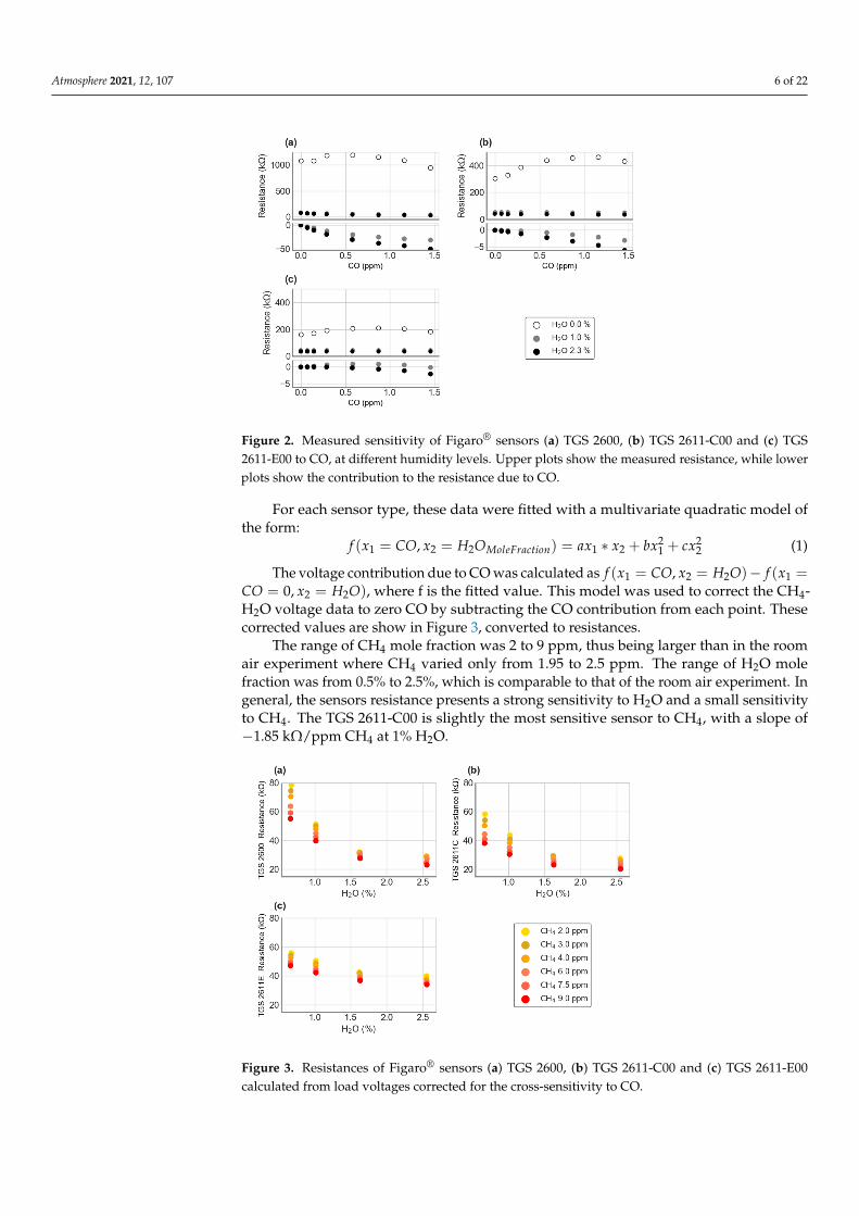
To account for the systematic error of the Figaro® resistances sensitivities to CH4 andH2O, caused by the different CO levels in the two CH4 target tanks, the sensors’ sensitivitiesto CO and H2O were separately measured and used to correct the data. In Figure 2, foreach Figaro® type, the upper plot shows the measured voltage across the load resistor forchanging CO mole fraction, at each of the three humidity levels 0, 1 and 2.3% mole fraction.The lower plot shows how much the Figaro® voltages increased above the baseline voltage,where the baseline is the voltage at zero CO and is a function of the humidity.

Atmosphere 2021, 12, 107 6 of 22

Figure 2. Measured sensitivity of Figaro® sensors (a) TGS 2600, (b) TGS 2611-C00 and (c) TGS2611-E00 to CO, at different humidity levels. Upper plots show the measured resistance, while lowerplots show the contribution to the resistance due to CO.

For each sensor type, these data were fitted with a multivariate quadratic model ofthe form:

f (x1 = CO, x2 = H2OMoleFraction) = ax1 ∗ x2 + bx21 + cx2

2 (1)

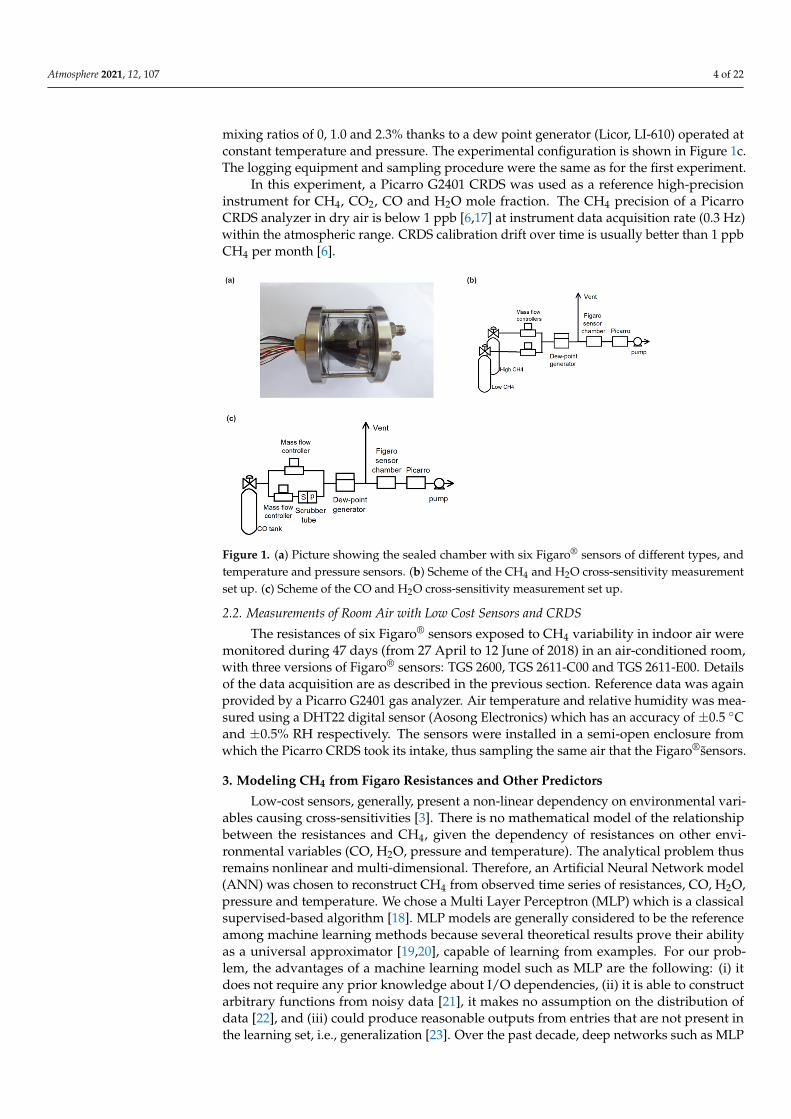
The voltage contribution due to CO was calculated as f (x1 = CO, x2 = H2O)− f (x1 =CO = 0, x2 = H2O), where f is the fitted value. This model was used to correct the CH4-H2O voltage data to zero CO by subtracting the CO contribution from each point. Thesecorrected values are show in Figure 3, converted to resistances.

The range of CH4 mole fraction was 2 to 9 ppm, thus being larger than in the roomair experiment where CH4 varied only from 1.95 to 2.5 ppm. The range of H2O molefraction was from 0.5% to 2.5%, which is comparable to that of the room air experiment. Ingeneral, the sensors resistance presents a strong sensitivity to H2O and a small sensitivityto CH4. The TGS 2611-C00 is slightly the most sensitive sensor to CH4, with a slope of−1.85 kΩ/ppm CH4 at 1% H2O.

Figure 3. Resistances of Figaro® sensors (a) TGS 2600, (b) TGS 2611-C00 and (c) TGS 2611-E00calculated from load voltages corrected for the cross-sensitivity to CO.

Atmosphere 2021, 12, 107 7 of 22

4.2. Data Pre-Processing for MLP Model

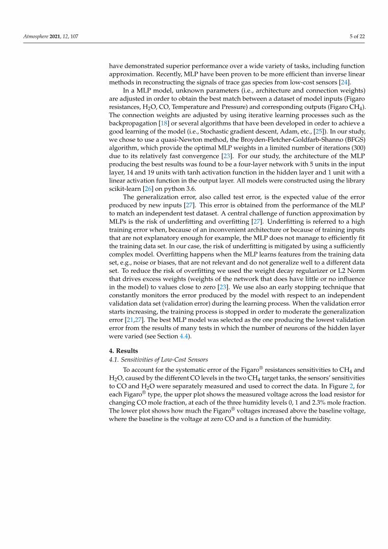
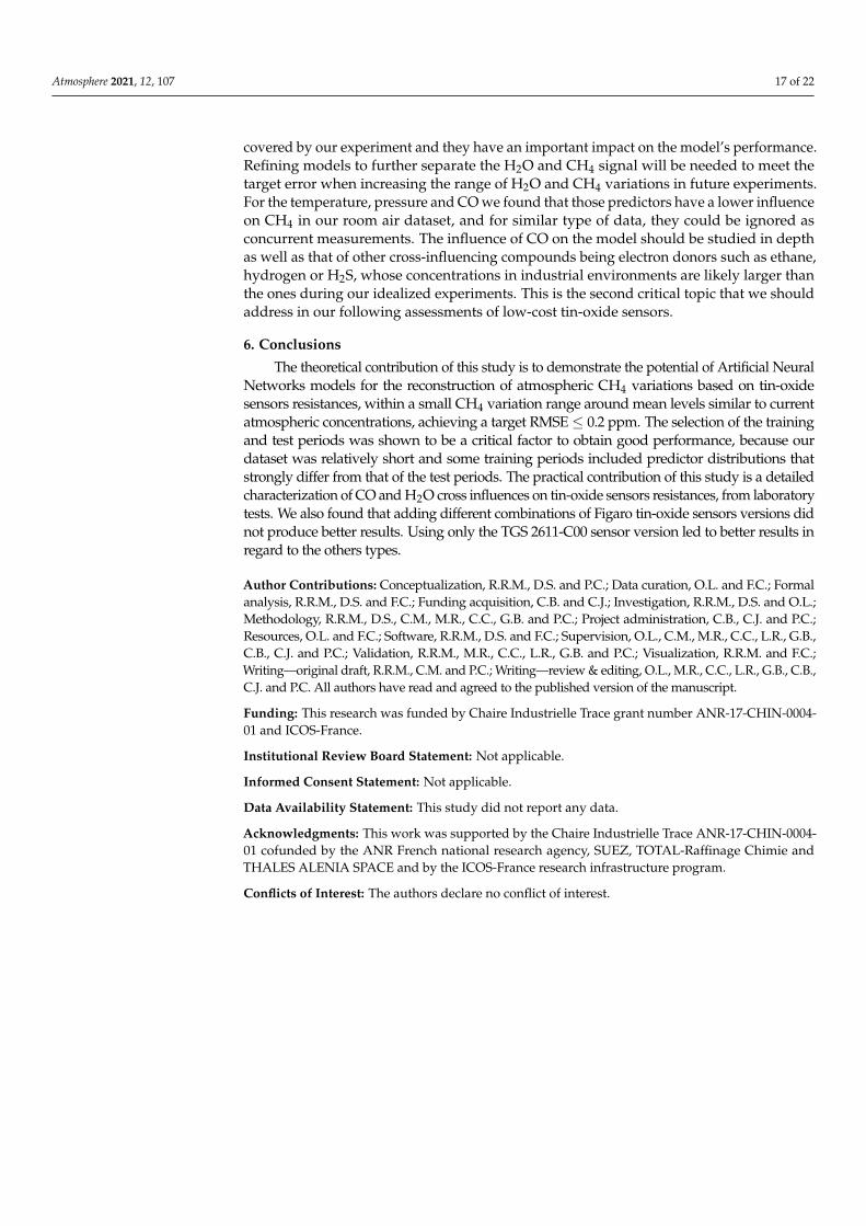
The data pre-processing scheme for the MLP model is summarized in Figure 4. Wefiltered the input and output data by removing NaN values and observations by anunknown source in the room that resulted in clear spikes of the TGS resistances. Thisresulted in 49,103 observations at a resolution of 1-min or 34 days of measurements. Foreach of the independent input variables, a low pass Savitzky-Golay Filter has been appliedto remove high frequencies corresponding to fluctuations of sensor measurements (1 minvariations) and a median filter has been used to remove the effect produced by the lowpass filter on gaps [28]. These filters have been not applied to the output data becausethe CH4 observations provided by the Picarro are not characterized by high frequencyvariations and because we wanted to keep the output data used for the training of theMLP as close as possible to the original data set. Figure A1 shows a comparison betweenthe raw signal and the filtered signal for one day of data. Because input variables havedifferent units and scales that could affect the relative sensitivities of the MLP with respectto each variable, they were normalized with a robust scaler which considers the statisticaldispersion of the observations by, removing the median and scaling the data according to aquantile range [29]. We used this scaler in order to prevent that outliers could affect therelative importance of each variable in the model, with that filtered dataset, we created twosub-sets of data to train and evaluate the MLP model. A training set always contained 70%of the entire dataset, the remaining 30% being the cross-validation dataset.

Figure 4. Data preprocessing and sub setting for the training and cross-validation of the Multi-LayerPerceptron model.

4.3. Room Air Measurements

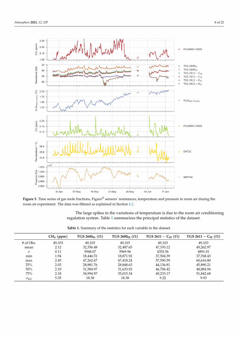
In Figure 5 are shown the smoothed time series on a time step of 1 min after a lowpass filtering (see Section 4.2) of room CH4 from the CRDS analyzer, resistances fromeach Figaro® CO from CRDS, room temperature of the DHT22 sensor, and pressure ofthe BMP180 sensor. H2O mole fraction (in %) was computed from relative humidity andtemperature of the DHT22 sensor and atmospheric pressure of the BMP180 sensor usingRankine’s formula:

H2OMole Fraction = 100 ×(

RH100 × e

13.7−5120T+273.15

P100000 − RH

100 × e13.7−5120T+273.15

)(2)

where RH is the relative humidity in %, P the atmospheric pressure in Pa and T thetemperature in C.

Atmosphere 2021, 12, 107 8 of 22

Figure 5. Time series of gas mole fractions, Figaro® sensors’ resistances, temperature and pressure in room air during theroom air experiment. The data was filtered as explained in Section 4.2.

The large spikes in the variations of temperature is due to the room air conditioningregulation system. Table 1 summarizes the principal statistics of the dataset.

Table 1. Summary of the statistics for each variable in the dataset.

CH4 (ppm) TGS 260001 (Ω) TGS 260002 (Ω) TGS 2611 − C01 (Ω) TGS 2611 − C02 (Ω)

# of Obs. 49,103 49,103 49,103 49,103 49,103mean 2.12 32,356.48 32,487.65 47,193.12 49,262.97

σ 0.11 5948.07 5969.96 4352.56 4891.01min 1.94 18,446.51 18,871.92 37,504.39 37,768.43max 2.45 47,262.67 47,418.24 57,590.59 60,616.8025% 2.03 28,881.76 28,848.63 44,136.81 45,890.2150% 2.10 31,584.97 31,633.92 46,706.42 48,884.9475% 2.18 34,994.97 35,015.34 49,233.17 51,842.68σRel 5.35 18.38 18.38 9.22 9.93

Atmosphere 2021, 12, 107 9 of 22

Table 1. Cont.

TGS 2611 − E01 (Ω) TGS 2611 − E02 (Ω) H2OMole Fraction (%) CO [ppm] T (C) P (Pa)

# of Obs. 49,103 49,103 49,103 49,103 49,103 49,103mean 60,425.14 63,378.21 1.58 0.11 25.53 99,709.67

σ 3010.45 6234.00 0.27 0.02 0.46 420.74min 52,472.35 54,468.19 1.07 0.08 24.11 98,289.72max 79,018.36 93,671.74 2.07 0.24 27.15 100,528.7925% 58,255.57 59,549.05 1.38 0.10 25.29 99,406.2250% 60,227.14 61,428.60 1.52 0.11 25.52 99,698.5775% 61,792.62 64,557.91 1.87 0.12 25.74 100,004.34σRel 4.98 9.84 17.17 18.38 1.81 0.42

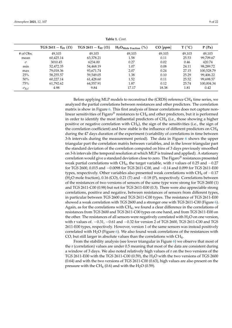
Before applying MLP models to reconstruct the (CRDS) reference CH4 time series, weanalyzed the partial correlations between resistances and other predictors. The correlationmatrix is show in Figure 6. This first analysis of linear correlations does not capture non-linear sensitivities of Figaro® resistances to CH4 and other predictors, but it is performedin order to identify the most influential predictors of CH4 (i.e., those showing a higherpositive or negative correlation with CH4), the sign of the sensitivities (i.e., the sign ofthe correlation coefficient) and how stable is the influence of different predictors on CH4during the 47 days duration of the experiment (variability of correlations in time between3-h intervals during the measurement period). The data in Figure 6 shows the uppertriangular part the correlation matrix between variables, and in the lower triangular partthe standard deviation of the correlation computed on bins of 3 days previously smoothedon 3-h intervals (the temporal resolution at which MLP is trained and applied). A stationarycorrelation would give a standard deviation close to zero. The Figaro® resistances presentedweak partial correlations with CH4, the target variable, with r values of 0.25 and −0.27for TGS 2600, 0.015 and −0.0098 for TGS 2611-C00, and −0.14 and 0.099 for TGS 2611-E00types, respectively. Other variables also presented weak correlations with CH4 of −0.17(H2O mole fraction), 0.16 (CO), 0.21 (T) and −0.18 (P), respectively. Correlations betweenof the resistances of two versions of sensors of the same type were strong for TGS 2600 (1)and TGS 2611-C00 (0.98) but not for TGS 2611-E00 (0.3). There were also appreciable strongcorrelations, positive and negative, between resistances of sensors from different types,in particular between TGS 2600 and TGS 2611-C00 types. The resistance of TGS 2611-E00showed a weak correlation with TGS 2600 and a stronger one with TGS 2611-C00 (Figure 6).Again, as for the correlations with CH4, we found a clear difference in the correlations ofresistances from TGS 2600 and TGS 2611-C00 types on one hand, and from TGS 2611-E00 onthe other. The resistances of all sensors were negatively correlated with H2O on one version,with r values of. −0.31, −0.61 and −0.32 for version 2 of TGS 2600, TGS 2611-C00 and TGS2611-E00 types, respectively. However, version 1 of the same sensors was instead positivelycorrelated with H2O (Figure 6). We also found weak correlations of the resistances withCO, but still larger in absolute values than the correlations with CH4.

From the stability analysis (see lower triangular in Figure 6) we observe that most ofthe r (correlation) values are under 0.5 meaning that most of the data are consistent duringa window of 3 days. We also noted relatively high values of r on the two versions of theTGS 2611-E00 with the TGS 2611-C00 (0.59), the H2O with the two versions of TGS 2600(0.64) and with the two versions of TGS 2611-C00 (0.63), high values are also present on thepressure with the CH4 (0.6) and with the H2O (0.59).

Atmosphere 2021, 12, 107 10 of 22

Figure 6. Partial correlation (r) matrix (upper triangular) and standard deviation of correlation forbins of 3 days previously smoothed at 20 min scale on 3 consecutive hours (lower triangular).

We conclude from this first analysis of correlations that, although there are correlations,between CH4 and the resistances of TGS 2600 and TGS 2611 sensors, such correlations aresmall and vary with time, which will make it challenging to reconstruct CH4 time serieswith linear models, and justifies a priori our choice of a MLP model. Same conclusionshave been drawn from previous studies [3,24].

4.4. Evaluation of the MLP Model

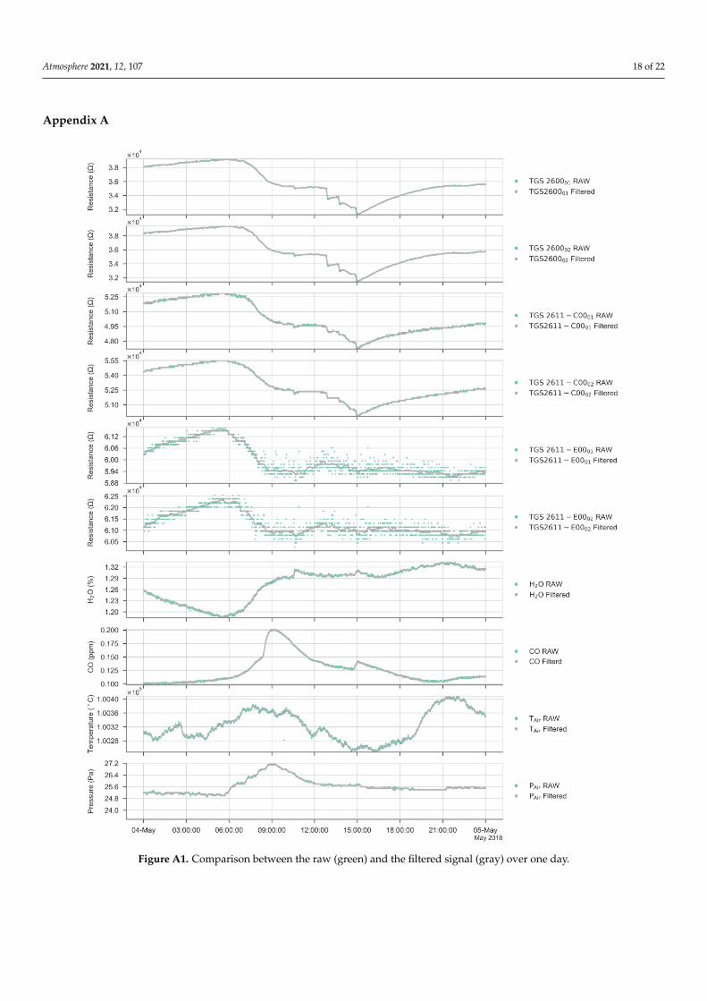
To assess the influence of the choice of the training period in the performance of theMLP, we defined over the whole data set 50 sliding training periods which contain 70% ofthe observations. The corresponding test sets contain thus 30% of the observations and theresults associated to the fits of the 50 MLPs are described in Figure 7.

The evaluation of the performance was based on 4 metrics: the RMSE on hourly data,the mean bias, the ratio between the spread of the predicted outputs from the model andthe spread of the true values (σModel/σData) and the correlation coefficient between theoutput of the model and the true values. On Figure 8 are presented two examples of theperformance of the MLP with different test periods, selected to represents a bad (period 50)and a good test (period 7) performance.

Atmosphere 2021, 12, 107 11 of 22

Figure 7. Performance of the MLP model for the 50 training and test periods. (a) RMSE on hourly data.(b) Mean bias. (c) Ratio between the spread of the predicted outputs (σModel) and the spread of thetrue values (σData). (d) Correlation coefficient between the predicted outputs and the reference values.

Figure 8. Time series showing a good (a) and a bad (b) performance of the MLP model for thetest period 7 and 50 respectively. In red, time series of the reference instrument, and in blue thereconstructed signal given by the MLP model. White background: observations used for the trainingstage. Blue background: observations used for the test stage.

Atmosphere 2021, 12, 107 12 of 22

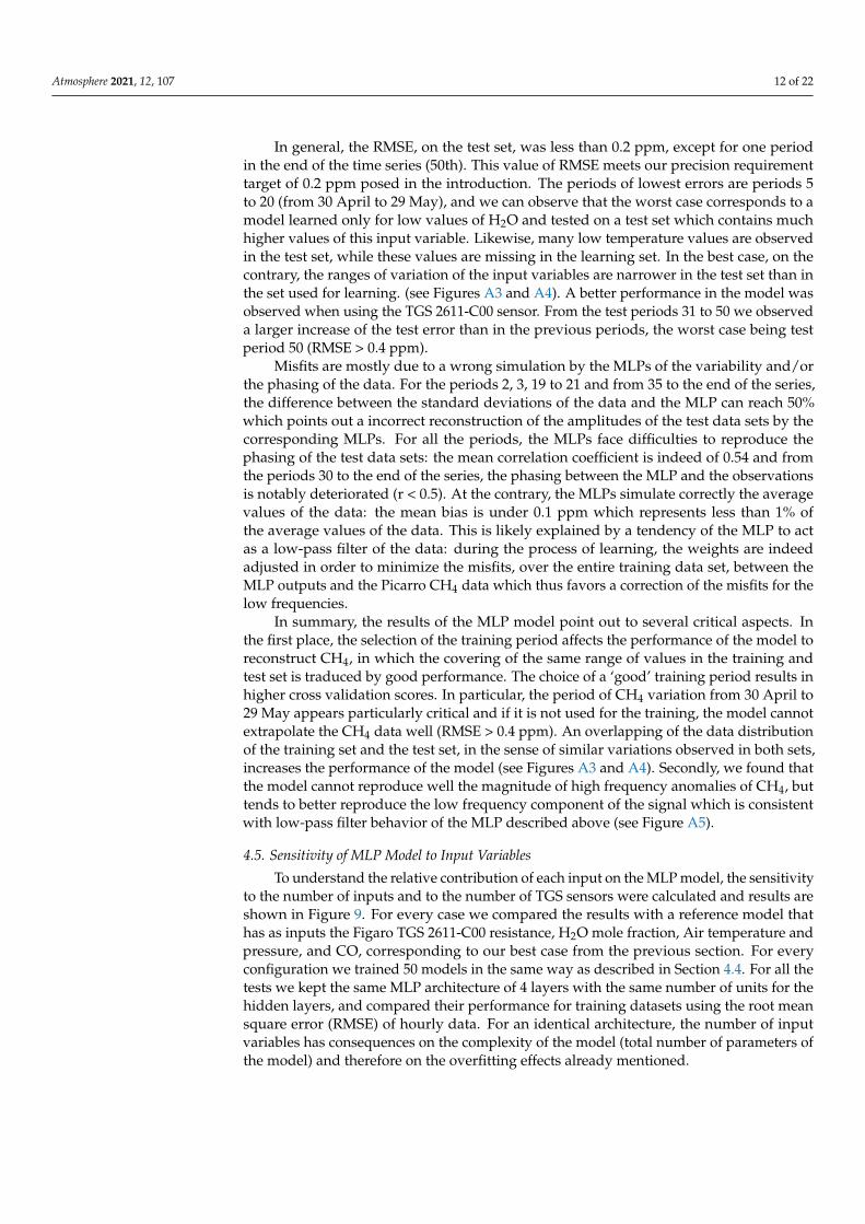
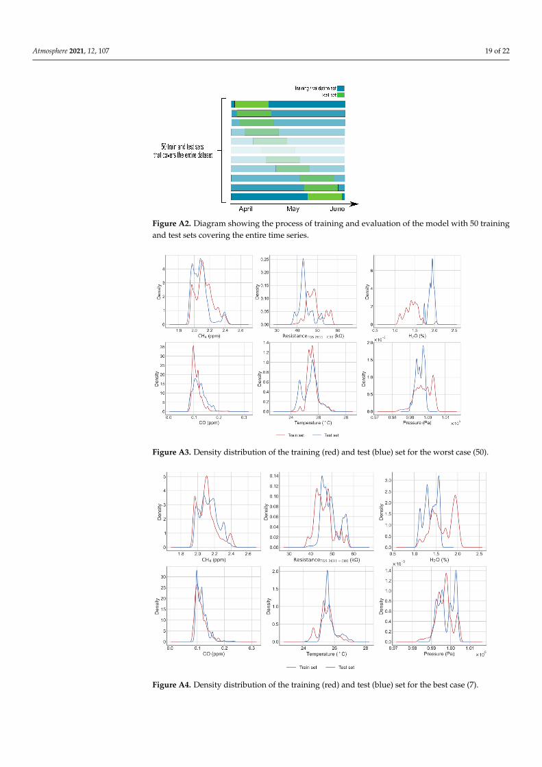
In general, the RMSE, on the test set, was less than 0.2 ppm, except for one periodin the end of the time series (50th). This value of RMSE meets our precision requirementtarget of 0.2 ppm posed in the introduction. The periods of lowest errors are periods 5to 20 (from 30 April to 29 May), and we can observe that the worst case corresponds to amodel learned only for low values of H2O and tested on a test set which contains muchhigher values of this input variable. Likewise, many low temperature values are observedin the test set, while these values are missing in the learning set. In the best case, on thecontrary, the ranges of variation of the input variables are narrower in the test set than inthe set used for learning. (see Figures A3 and A4). A better performance in the model wasobserved when using the TGS 2611-C00 sensor. From the test periods 31 to 50 we observeda larger increase of the test error than in the previous periods, the worst case being testperiod 50 (RMSE > 0.4 ppm).

Misfits are mostly due to a wrong simulation by the MLPs of the variability and/orthe phasing of the data. For the periods 2, 3, 19 to 21 and from 35 to the end of the series,the difference between the standard deviations of the data and the MLP can reach 50%which points out a incorrect reconstruction of the amplitudes of the test data sets by thecorresponding MLPs. For all the periods, the MLPs face difficulties to reproduce thephasing of the test data sets: the mean correlation coefficient is indeed of 0.54 and fromthe periods 30 to the end of the series, the phasing between the MLP and the observationsis notably deteriorated (r < 0.5). At the contrary, the MLPs simulate correctly the averagevalues of the data: the mean bias is under 0.1 ppm which represents less than 1% ofthe average values of the data. This is likely explained by a tendency of the MLP to actas a low-pass filter of the data: during the process of learning, the weights are indeedadjusted in order to minimize the misfits, over the entire training data set, between theMLP outputs and the Picarro CH4 data which thus favors a correction of the misfits for thelow frequencies.

In summary, the results of the MLP model point out to several critical aspects. Inthe first place, the selection of the training period affects the performance of the model toreconstruct CH4, in which the covering of the same range of values in the training andtest set is traduced by good performance. The choice of a ‘good’ training period results inhigher cross validation scores. In particular, the period of CH4 variation from 30 April to29 May appears particularly critical and if it is not used for the training, the model cannotextrapolate the CH4 data well (RMSE > 0.4 ppm). An overlapping of the data distributionof the training set and the test set, in the sense of similar variations observed in both sets,increases the performance of the model (see Figures A3 and A4). Secondly, we found thatthe model cannot reproduce well the magnitude of high frequency anomalies of CH4, buttends to better reproduce the low frequency component of the signal which is consistentwith low-pass filter behavior of the MLP described above (see Figure A5).

4.5. Sensitivity of MLP Model to Input Variables

To understand the relative contribution of each input on the MLP model, the sensitivityto the number of inputs and to the number of TGS sensors were calculated and results areshown in Figure 9. For every case we compared the results with a reference model thathas as inputs the Figaro TGS 2611-C00 resistance, H2O mole fraction, Air temperature andpressure, and CO, corresponding to our best case from the previous section. For everyconfiguration we trained 50 models in the same way as described in Section 4.4. For all thetests we kept the same MLP architecture of 4 layers with the same number of units for thehidden layers, and compared their performance for training datasets using the root meansquare error (RMSE) of hourly data. For an identical architecture, the number of inputvariables has consequences on the complexity of the model (total number of parameters ofthe model) and therefore on the overfitting effects already mentioned.

Atmosphere 2021, 12, 107 13 of 22

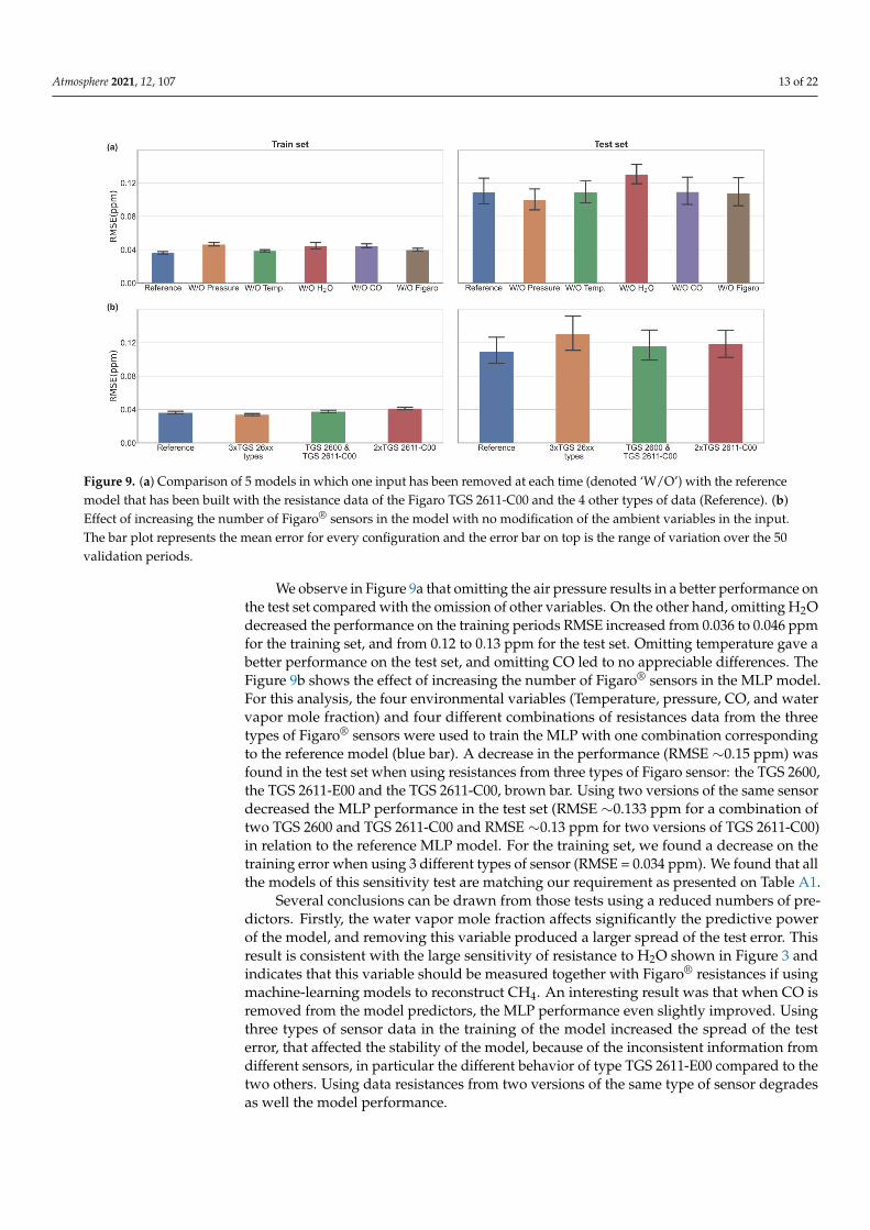
Figure 9. (a) Comparison of 5 models in which one input has been removed at each time (denoted ‘W/O’) with the referencemodel that has been built with the resistance data of the Figaro TGS 2611-C00 and the 4 other types of data (Reference). (b)Effect of increasing the number of Figaro® sensors in the model with no modification of the ambient variables in the input.The bar plot represents the mean error for every configuration and the error bar on top is the range of variation over the 50validation periods.

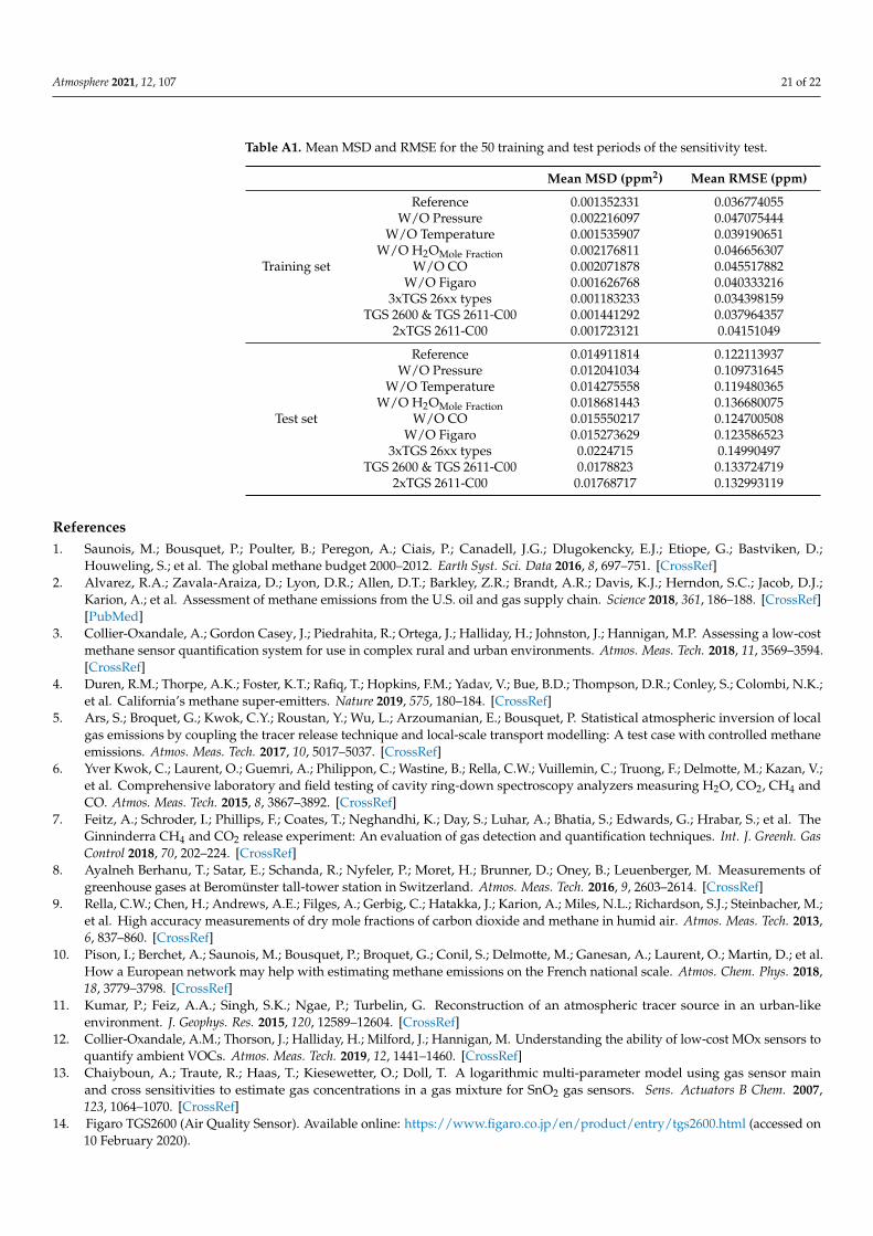
We observe in Figure 9a that omitting the air pressure results in a better performance onthe test set compared with the omission of other variables. On the other hand, omitting H2Odecreased the performance on the training periods RMSE increased from 0.036 to 0.046 ppmfor the training set, and from 0.12 to 0.13 ppm for the test set. Omitting temperature gave abetter performance on the test set, and omitting CO led to no appreciable differences. TheFigure 9b shows the effect of increasing the number of Figaro® sensors in the MLP model.For this analysis, the four environmental variables (Temperature, pressure, CO, and watervapor mole fraction) and four different combinations of resistances data from the threetypes of Figaro® sensors were used to train the MLP with one combination correspondingto the reference model (blue bar). A decrease in the performance (RMSE ∼0.15 ppm) wasfound in the test set when using resistances from three types of Figaro sensor: the TGS 2600,the TGS 2611-E00 and the TGS 2611-C00, brown bar. Using two versions of the same sensordecreased the MLP performance in the test set (RMSE ∼0.133 ppm for a combination oftwo TGS 2600 and TGS 2611-C00 and RMSE ∼0.13 ppm for two versions of TGS 2611-C00)in relation to the reference MLP model. For the training set, we found a decrease on thetraining error when using 3 different types of sensor (RMSE = 0.034 ppm). We found that allthe models of this sensitivity test are matching our requirement as presented on Table A1.

Several conclusions can be drawn from those tests using a reduced numbers of pre-dictors. Firstly, the water vapor mole fraction affects significantly the predictive powerof the model, and removing this variable produced a larger spread of the test error. Thisresult is consistent with the large sensitivity of resistance to H2O shown in Figure 3 andindicates that this variable should be measured together with Figaro® resistances if usingmachine-learning models to reconstruct CH4. An interesting result was that when CO isremoved from the model predictors, the MLP performance even slightly improved. Usingthree types of sensor data in the training of the model increased the spread of the testerror, that affected the stability of the model, because of the inconsistent information fromdifferent sensors, in particular the different behavior of type TGS 2611-E00 compared to thetwo others. Using data resistances from two versions of the same type of sensor degradesas well the model performance.

Atmosphere 2021, 12, 107 14 of 22

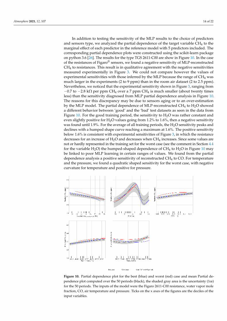
In addition to testing the sensitivity of the MLP results to the choice of predictorsand sensors type, we analyzed the partial dependence of the target variable CH4 to themarginal effect of each predictor in the reference model with 5 predictors included. Thecorresponding partial dependence plots were constructed using the scikit-learn packageon python 3.6 [26]. The results for the type TGS 2611-C00 are show in Figure 10. In the caseof the resistances of Figaro® sensors, we found a negative sensitivity of MLP-reconstructedCH4 to resistances. This result is in qualitative agreement with the negative sensitivitiesmeasured experimentally in Figure 3. We could not compare however the values ofexperimental sensitivities with those inferred by the MLP because the range of CH4 wasmuch larger in the experiments (2 to 9 ppm) than in the room air dataset (2 to 2.5 ppm).Nevertheless, we noticed that the experimental sensitivity shown in Figure 3, ranging from−0.7 to −2.8 kΩ per ppm CH4 over a 7 ppm CH4 is much smaller (about twenty timesless) than the sensitivity diagnosed from MLP partial dependence analysis in Figure 10.The reasons for this discrepancy may be due to sensors aging or to an over-estimationby the MLP model. The partial dependence of MLP-reconstructed CH4 to H2O showeda different behavior between ’good’ and the ’bad’ test datasets as seen in the data fromFigure 10. For the good training period, the sensitivity to H2O was rather constant andeven slightly positive for H2O values going from 1.2% to 1.6%, then a negative sensitivitywas found until 1.9%. For the average of all training periods, the H2O sensitivity peaks anddeclines with a humped shape curve reaching a maximum at 1.6%. The positive sensitivitybelow 1.6% is consistent with experimental sensitivities of Figure 3, in which the resistancedecreases for an increase of H2O and decreases when CH4 increases. Since some values arenot or hardly represented in the training set for the worst case (see the comment in Section 4.4for the variable H2O) the humped-shaped dependence of CH4 to H2O in Figure 10 maybe linked to poor MLP learning in certain ranges of values. We found from the partialdependence analysis a positive sensitivity of reconstructed CH4 to CO. For temperatureand the pressure, we found a quadratic shaped sensitivity for the worst case, with negativecurvature for temperature and positive for pressure.

Figure 10. Partial dependence plot for the best (blue) and worst (red) case and mean Partial de-pendence plot computed over the 50 periods (black), the shaded gray area is the uncertainty (1œ)for the 50 periods. The inputs of the model were the Figaro 2611-C00 resistance, water vapor molefraction, CO, air temperature and pressure. Ticks on the x axes of the figures are the deciles of theinput variables.

Atmosphere 2021, 12, 107 15 of 22

The bivariate partial dependence plots in Figure 11a show the dependence of theMLP-reconstructed CH4 on the joint values of resistance and the other variables for thebest test case (see Figure 11b for the worst case). On this best case, we observe that there isa high dependence to resistance of the MLP-reconstructed CH4 for values of H2O under1.6%, whereas for values between 1.6% and 1.8% the dependence flattens off. ConsideringCO and temperature, we found that the MLP model is highly dependent of resistances forvalues under 0.15 ppm of CO and temperature under 26.5 C, for the best and the worstcases for CO. Finally, the model seems to be sensitive to pressure when the resistance variesover 48 kΩ and under 44 kΩ.

Figure 11. Bivariate partial dependence plot for the TGS 2611-C00 sensor versus H2O mole fraction, CO, air temperatureand pressure. (a) Partial Dependence Plot (PDP) for the model trained in the best case scenario and (b) Partial DependencePlot (PDP) for the worst case scenario. Ticks on the x and y axes of the figures are the deciles of the input variables.

5. Discussion

Few studies have tried to use machine-learning models to reconstruct the variability andthe concentration of greenhouse gases from low cost sensors [30]. In the work of [31,31,32])several field calibration methods for low cost sensors were explored: Linear and multilinearregression and Artificial Neural Network (ANN), for five trace gases (O3, NO2, NO, COand CO2) measured by metal oxide, electrochemical and miniaturized infrared sensorsover five months. They concluded that the best calibration method was ANN and thatthe use of different types of sensors could help the ANN to solve the cross sensitivities.Here, we found that only using Figaro® TGS sensors, even from different types, it was notpossible to make a good reconstruction of the signal without concurrent measurements ofother environmental variables, because the sensors had a high cross sensitivity to watervapor, aggravated by differences on the distribution of the H2O density for the trainingand test set.

The study of Esposito et al. [33] compared the performance of feed forward neuralnetworks (FFNN) with dynamical neural network (DNN) in the calibration of three tracegases (NOx, NO2 and O3) measured with low cost sensors over five weeks. They found thatDNN was significantly more accurate than FFNN in the reconstruction of high variations

Atmosphere 2021, 12, 107 16 of 22

of concentrations. As explained on Section 3, the high capacity problem in which themore complex models tend to overfit needs to be treated carefully, thus we tested a seriesof combinations of number of units and number of layers obtaining an architecture of 2hidden layers the more adapted to this problem, our limited dataset also restraints a morecomplex model.

Cordero et al. [34] worked on a two-step calibration process of NO2, NO and O3from low cost sensors. They applied a first multilinear regression considering all thepredictors, then the error of the multilinear regression was introduced as an input, inaddition to the others predictors, to a supervised machine learning algorithm (SupportVector Machine—SVM, random forest or ANN) to reconstruct the concentration of tracegases. They concluded that globally SVM and ANN performed well in the reconstructionof the concentrations in all the cases over a threshold (40 µg/m3). For data below thatthreshold, the random forest was the best model to reconstruct the signal. As a universalapproximator, we decided to use MLP in our study for the reconstruction of small variationsof CH4 measurements at levels around ambient air values, and we did not test the limits ofthis type of model in presence of high variations of our signal, such as CH4 spikes of severalppm encountered when measuring air at a point nearby an industrial site. This questionremains open for a future study with a specific dataset of CH4 that contains spikes.

Casey et al. [24] compared the performance of direct linear models, inverse linearmodels and ANN models over three months of data of ambient air in a region influencedby oil and gas production. Their main results pointed that the ANN model, when appliedto CH4 and CO observations, gave better performance (RMSE = 0.13 ppm over a month)than the direct and inverse linear models, due to the smaller dynamic range from theirobservations. For our study, a linear model could not be applied due to nonlinear rela-tionships between predictors with the target CH4 signal. With a careful selection of theMLP model, our results indicate that the MLP model provided performances that meetour target requirement of an error of 0.1 to 0.2 ppm for hourly average CH4, except duringperiods when the distribution of training data was too different from the one of the testdata (80% on the last test period of the cross validation). This illustrates the critical aspectfor MLP and other machine learning models to use large datasets, with all the space ofpredictors being covered by training datasets, to reach good cross validation performance.

Eugster et al. [35] conducted a long term evaluation of the Figaro® TGS 2600 over sevenyears at Toolik Lake in Alaska; they proposed a multilinear model to calibrate the voltagesignal from the sensor including other environmental variables such as air temperatureand absolute humidity. The calibration methods were assessed under summer and winterconditions and compared their proposed model with an ANN. Eugster et al. [35] foundsatisfying agreement on 30 min average observations for the multilinear model (R2 = 0.424).They reported a more balanced performance of the ANN on cold conditions (winter), butthey not find a substantial difference between their proposed model and the ANN. Theyconcluded that ANN would outperform linear models if other driving variables wereincluded to the model.

Riddick et al. [36] conducted an experiment to investigate the potential of Figaro®

TGS 2600 to measure CH4 mixing ratios in ranges between 2 and 10 ppm, assess the longterm measurements over 3 months and estimate the emissions from a natural gas pointsource. Calibration of the sensor was derived from a non linear relationship giving the bestagreement with the reference measurements when computing the time averaged concen-tration with a uncertainty of ±0.01 ppm. The authors observed that reliably measurementsof CH4 was in the range of 1.8 to 6 ppm and suggest that calibrations need to be derivedfor each individual sensor.

From the results of the sensitivity tests to removing predictors one at a time, and thepartial dependence plots providing the sensitivities of the MLP modeled CH4 to individualpredictors we could observe the importance of the water vapor as a critical input for themodels. This is mainly due to the high sensitivity for the TGS sensors to H2O confirmedby our experimental data. Variations of H2O in the field are typically larger than the ones

Atmosphere 2021, 12, 107 17 of 22

covered by our experiment and they have an important impact on the model’s performance.Refining models to further separate the H2O and CH4 signal will be needed to meet thetarget error when increasing the range of H2O and CH4 variations in future experiments.For the temperature, pressure and CO we found that those predictors have a lower influenceon CH4 in our room air dataset, and for similar type of data, they could be ignored asconcurrent measurements. The influence of CO on the model should be studied in depthas well as that of other cross-influencing compounds being electron donors such as ethane,hydrogen or H2S, whose concentrations in industrial environments are likely larger thanthe ones during our idealized experiments. This is the second critical topic that we shouldaddress in our following assessments of low-cost tin-oxide sensors.

6. Conclusions

The theoretical contribution of this study is to demonstrate the potential of Artificial NeuralNetworks models for the reconstruction of atmospheric CH4 variations based on tin-oxidesensors resistances, within a small CH4 variation range around mean levels similar to currentatmospheric concentrations, achieving a target RMSE ≤ 0.2 ppm. The selection of the trainingand test periods was shown to be a critical factor to obtain good performance, because ourdataset was relatively short and some training periods included predictor distributions thatstrongly differ from that of the test periods. The practical contribution of this study is a detailedcharacterization of CO and H2O cross influences on tin-oxide sensors resistances, from laboratorytests. We also found that adding different combinations of Figaro tin-oxide sensors versions didnot produce better results. Using only the TGS 2611-C00 sensor version led to better results inregard to the others types.

Author Contributions: Conceptualization, R.R.M., D.S. and P.C.; Data curation, O.L. and F.C.; Formalanalysis, R.R.M., D.S. and F.C.; Funding acquisition, C.B. and C.J.; Investigation, R.R.M., D.S. and O.L.;Methodology, R.R.M., D.S., C.M., M.R., C.C., G.B. and P.C.; Project administration, C.B., C.J. and P.C.;Resources, O.L. and F.C.; Software, R.R.M., D.S. and F.C.; Supervision, O.L., C.M., M.R., C.C., L.R., G.B.,C.B., C.J. and P.C.; Validation, R.R.M., M.R., C.C., L.R., G.B. and P.C.; Visualization, R.R.M. and F.C.;Writing—original draft, R.R.M., C.M. and P.C.; Writing—review & editing, O.L., M.R., C.C., L.R., G.B., C.B.,C.J. and P.C. All authors have read and agreed to the published version of the manuscript.

Funding: This research was funded by Chaire Industrielle Trace grant number ANR-17-CHIN-0004-01 and ICOS-France.

Institutional Review Board Statement: Not applicable.

Informed Consent Statement: Not applicable.

Data Availability Statement: This study did not report any data.

Acknowledgments: This work was supported by the Chaire Industrielle Trace ANR-17-CHIN-0004-01 cofunded by the ANR French national research agency, SUEZ, TOTAL-Raffinage Chimie andTHALES ALENIA SPACE and by the ICOS-France research infrastructure program.

Conflicts of Interest: The authors declare no conflict of interest.

Atmosphere 2021, 12, 107 18 of 22

Appendix A

Figure A1. Comparison between the raw (green) and the filtered signal (gray) over one day.

Atmosphere 2021, 12, 107 19 of 22

Figure A2. Diagram showing the process of training and evaluation of the model with 50 trainingand test sets covering the entire time series.

Figure A3. Density distribution of the training (red) and test (blue) set for the worst case (50).

Figure A4. Density distribution of the training (red) and test (blue) set for the best case (7).

Atmosphere 2021, 12, 107 20 of 22

Figure A5. Output of the model for a smoothed signal of 12 h (a) and 24 h (b).

Figure A6. Partial correlation (r) matrix (upper triangular) and standard deviation of correlation forbins of 3 days previously smoothed at an hourly scale (lower triangular).

Atmosphere 2021, 12, 107 21 of 22

Table A1. Mean MSD and RMSE for the 50 training and test periods of the sensitivity test.

Mean MSD (ppm2) Mean RMSE (ppm)

Reference 0.001352331 0.036774055W/O Pressure 0.002216097 0.047075444

W/O Temperature 0.001535907 0.039190651W/O H2OMole Fraction 0.002176811 0.046656307

Training set W/O CO 0.002071878 0.045517882W/O Figaro 0.001626768 0.040333216

3xTGS 26xx types 0.001183233 0.034398159TGS 2600 & TGS 2611-C00 0.001441292 0.037964357

2xTGS 2611-C00 0.001723121 0.04151049

Reference 0.014911814 0.122113937W/O Pressure 0.012041034 0.109731645

W/O Temperature 0.014275558 0.119480365W/O H2OMole Fraction 0.018681443 0.136680075

Test set W/O CO 0.015550217 0.124700508W/O Figaro 0.015273629 0.123586523

3xTGS 26xx types 0.0224715 0.14990497TGS 2600 & TGS 2611-C00 0.0178823 0.133724719

2xTGS 2611-C00 0.01768717 0.132993119

References1. Saunois, M.; Bousquet, P.; Poulter, B.; Peregon, A.; Ciais, P.; Canadell, J.G.; Dlugokencky, E.J.; Etiope, G.; Bastviken, D.;

Houweling, S.; et al. The global methane budget 2000–2012. Earth Syst. Sci. Data 2016, 8, 697–751. [CrossRef]2. Alvarez, R.A.; Zavala-Araiza, D.; Lyon, D.R.; Allen, D.T.; Barkley, Z.R.; Brandt, A.R.; Davis, K.J.; Herndon, S.C.; Jacob, D.J.;

Karion, A.; et al. Assessment of methane emissions from the U.S. oil and gas supply chain. Science 2018, 361, 186–188. [CrossRef][PubMed]

3. Collier-Oxandale, A.; Gordon Casey, J.; Piedrahita, R.; Ortega, J.; Halliday, H.; Johnston, J.; Hannigan, M.P. Assessing a low-costmethane sensor quantification system for use in complex rural and urban environments. Atmos. Meas. Tech. 2018, 11, 3569–3594.[CrossRef]

4. Duren, R.M.; Thorpe, A.K.; Foster, K.T.; Rafiq, T.; Hopkins, F.M.; Yadav, V.; Bue, B.D.; Thompson, D.R.; Conley, S.; Colombi, N.K.;et al. California’s methane super-emitters. Nature 2019, 575, 180–184. [CrossRef]

5. Ars, S.; Broquet, G.; Kwok, C.Y.; Roustan, Y.; Wu, L.; Arzoumanian, E.; Bousquet, P. Statistical atmospheric inversion of localgas emissions by coupling the tracer release technique and local-scale transport modelling: A test case with controlled methaneemissions. Atmos. Meas. Tech. 2017, 10, 5017–5037. [CrossRef]

6. Yver Kwok, C.; Laurent, O.; Guemri, A.; Philippon, C.; Wastine, B.; Rella, C.W.; Vuillemin, C.; Truong, F.; Delmotte, M.; Kazan, V.;et al. Comprehensive laboratory and field testing of cavity ring-down spectroscopy analyzers measuring H2O, CO2, CH4 andCO. Atmos. Meas. Tech. 2015, 8, 3867–3892. [CrossRef]

7. Feitz, A.; Schroder, I.; Phillips, F.; Coates, T.; Neghandhi, K.; Day, S.; Luhar, A.; Bhatia, S.; Edwards, G.; Hrabar, S.; et al. TheGinninderra CH4 and CO2 release experiment: An evaluation of gas detection and quantification techniques. Int. J. Greenh. GasControl 2018, 70, 202–224. [CrossRef]

8. Ayalneh Berhanu, T.; Satar, E.; Schanda, R.; Nyfeler, P.; Moret, H.; Brunner, D.; Oney, B.; Leuenberger, M. Measurements ofgreenhouse gases at Beromünster tall-tower station in Switzerland. Atmos. Meas. Tech. 2016, 9, 2603–2614. [CrossRef]

9. Rella, C.W.; Chen, H.; Andrews, A.E.; Filges, A.; Gerbig, C.; Hatakka, J.; Karion, A.; Miles, N.L.; Richardson, S.J.; Steinbacher, M.;et al. High accuracy measurements of dry mole fractions of carbon dioxide and methane in humid air. Atmos. Meas. Tech. 2013,6, 837–860. [CrossRef]

10. Pison, I.; Berchet, A.; Saunois, M.; Bousquet, P.; Broquet, G.; Conil, S.; Delmotte, M.; Ganesan, A.; Laurent, O.; Martin, D.; et al.How a European network may help with estimating methane emissions on the French national scale. Atmos. Chem. Phys. 2018,18, 3779–3798. [CrossRef]

11. Kumar, P.; Feiz, A.A.; Singh, S.K.; Ngae, P.; Turbelin, G. Reconstruction of an atmospheric tracer source in an urban-likeenvironment. J. Geophys. Res. 2015, 120, 12589–12604. [CrossRef]

12. Collier-Oxandale, A.M.; Thorson, J.; Halliday, H.; Milford, J.; Hannigan, M. Understanding the ability of low-cost MOx sensors toquantify ambient VOCs. Atmos. Meas. Tech. 2019, 12, 1441–1460. [CrossRef]

13. Chaiyboun, A.; Traute, R.; Haas, T.; Kiesewetter, O.; Doll, T. A logarithmic multi-parameter model using gas sensor mainand cross sensitivities to estimate gas concentrations in a gas mixture for SnO2 gas sensors. Sens. Actuators B Chem. 2007,123, 1064–1070. [CrossRef]

14. Figaro TGS2600 (Air Quality Sensor). Available online: https://www.figaro.co.jp/en/product/entry/tgs2600.html (accessed on10 February 2020).

Atmosphere 2021, 12, 107 22 of 22

15. Figaro TGS2611-C00 (Methane Sensor). Available online: https://www.figaro.co.jp/en/product/entry/tgs2611-c00.html (ac-cessed on 10 February 2020).

16. Xueref-Remy, I.; Zazzeri, G.; Bréon, F.; Vogel, F.; Ciais, P.; Lowry, D.; Nisbet, E. Anthropogenic methane plume detection frompoint sources in the Paris megacity area and characterization of their δ13C signature. Atmos. Environ. 2019, 117055. [CrossRef]

17. Picarro Inc. G2401 Analyzer for User’s Guide; Picarro Inc.: Santa Clara, CA, USA, 2017.18. Rumelhart, D.E.; Hinton, G.E.; Williams, R.J. Learning representation by back-propagating errors. Nature 1986, 323, 533–536.

[CrossRef]19. Cybenko, G. Approximation by superpositions of a sigmoidal function. Math. Control Signals Syst. 1989, 2, 303–314. [CrossRef]20. Hornik, K.; Stinchcombe, M.; White, H. Multilayer feedforward networks are universal approximators. Neural Netw. 1989,

2, 359–366. [CrossRef]21. Bishop, C.; Bishop, P.; Hinton, G.; Press, O.U. Neural Networks for Pattern Recognition; Advanced Texts in Econometrics; Clarendon

Press: Oxford, UK, 1995.22. Gardner, M.W.; Dorling, S.R. Artificial neural networks (the multilayer perceptron)—A review of applications in the atmospheric

sciences. Atmos. Environ. 1998, 32, 2627–2636. [CrossRef]23. Haykin, S. Neural Networks: A Comprehensive Foundation; Prentice Hall PTR: Upper Saddle River, NJ, USA, 1994.24. Casey, J.G.; Collier-Oxandale, A.; Hannigan, M. Performance of artificial neural networks and linear models to quantify 4 trace

gas species in an oil and gas production region with low-cost sensors. Sens. Actuators B Chem. 2019, 283, 504–514. [CrossRef]25. Géron, A. Hands-On Machine Learning with Scikit-Learn, Keras, and TensorFlow: Concepts, Tools, and Techniques to Build Intelligent

Systems; O’Reilly Media: Bodega Avenue Sebastopol, CA, USA, 2019.26. Varoquaux, G.; Buitinck, L.; Louppe, G.; Grisel, O.; Pedregosa, F.; Mueller, A. Scikit-learn. Getmobile Mob. Comput. Commun. 2015,

19, 29–33. [CrossRef]27. Goodfellow, I.; Bengio, Y.; Courville, A. Deep Learning; MIT Press: Cambridge, MA, USA, 2016. Available online: http:

//www.deeplearningbook.org (accessed on 18 April 2020).28. Press, W.H.; Teukolsky, S.A. Savitzky-Golay Smoothing Filters. Comput. Phys. 1990, 4, 669. [CrossRef]29. Hagan, M.; Demuth, H.; Beale, M.; De Jesús, O. Neural Network Design; Martin Hagan: Pittsburgh, PA, USA, 2014.30. Shahid, A.; Choi, J.H.; Rana, A.U.H.S.; Kim, H.S. Least squares neural network-based wireless E-nose system using an SnO2

sensor array. Sensors 2018, 18, 1446. [CrossRef] [PubMed]31. Spinelle, L.; Gerboles, M.; Villani, M.G.; Aleixandre, M.; Bonavitacola, F. Field calibration of a cluster of low-cost available sensors

for air quality monitoring. Part A: Ozone and nitrogen dioxide. Sens. Actuators B Chem. 2015, 215, 249–257. [CrossRef]32. Spinelle, L.; Gerboles, M.; Villani, M.G.; Aleixandre, M.; Bonavitacola, F. Field calibration of a cluster of low-cost commercially

available sensors for air quality monitoring. Part B: NO, CO and CO2. Sens. Actuators B Chem. 2017, 238, 706–715. [CrossRef]33. Esposito, E.; De Vito, S.; Salvato, M.; Bright, V.; Jones, R.L.; Popoola, O. Dynamic neural network architectures for on field

stochastic calibration of indicative low cost air quality sensing systems. Sens. Actuators B Chem. 2016, 231, 701–713. [CrossRef]34. Cordero, J.M.; Borge, R.; Narros, A. Using statistical methods to carry out in field calibrations of low cost air quality sensors. Sens.

Actuators B Chem. 2018, 267, 245–254. [CrossRef]35. Eugster, W.; Laundre, J.; Eugster, J.; Kling, G.W. Long-term reliability of the Figaro TGS 2600 solid-state methane sensor under

low-Arctic conditions at Toolik Lake, Alaska. Atmos. Meas. Tech. 2020, 13, 2681–2695. [CrossRef]36. Riddick, S.N.; Mauzerall, D.L.; Celia, M.; Allen, G.; Pitt, J.; Kang, M.; Riddick, J.C. The calibration and deployment of a low-cost

methane sensor. Atmos. Environ. 2020, 230, 117440. [CrossRef]