The Places of Our Lives: Visiting Patterns and Automatic ...

1

The Places of Our Lives: Visiting Patterns andAutomatic Labeling from Longitudinal

Smartphone DataTrinh Minh Tri Do and Daniel Gatica-Perez, Member, IEEE

Abstract—The location tracking functionality of modern mobile devices provides unprecedented opportunity to the understanding ofindividual mobility in daily life. Instead of studying raw geographic coordinates, we are interested in understanding human mobilitypatterns based on sequences of place visits which encode, at a coarse resolution, most daily activities. This paper presents a study onplace characterization in people’s everyday life based on data recorded continuously by smartphones. First, we study human mobilityfrom sequences of place visits, including visiting patterns on different place categories. Second, we address the problem of automaticplace labeling from smartphone data without using any geo-location information. Our study on a large-scale data collected from 114smartphone users over 18 months confirms many intuitions, and also reveals findings regarding both regularly and novelty trends invisiting patterns. Considering the problem of place labeling with 10 place categories, we show that frequently visited places can berecognized reliably (over 80%) while it is much more challenging to recognize infrequent places.

Index Terms—smartphone data, human mobility, place extraction, place visit, place labeling, prediction

F

1 INTRODUCTIONLocation is a key feature for context-aware mobile ser-vices. In particular, the places in everyday life are the an-chors around which social networks like FourSquare andlocation sharing services like Facebook Places have beenbuilt and are exploited, enabled by the widespread use ofsmartphones, which allow to provide location explicitly(via check-ins) or to infer it from sensors [1], [2]. Giventhe importance that places play in our lives, it is notsurprising that current research is examining methods toautomatically characterize places and understand theirfunctions – from private to professional spaces and fromtransportation hubs to leisure sites [3], [4].

The availability of various forms of geolocation datacoming from mobile phones has allowed researchers tostudy human mobility at large scale in recent years.Human trajectories were used to characterize a law ofhuman motion from mobile cell-tower data in [5], how-ever the differences in travel distances and the inherentanisotropy of each trajectory must be corrected in orderto observe recurrent travel patterns. In another studyusing Foursquare data [6], it was shown that trips arenot explicitly dependent on physical distance but on theset of places satisfying the objective of the trip. Theseand other findings confirm that the concept of place –which has a central role in this paper– is key for studyingindividual mobility patterns.

When considering a user’s location traces as sequencesof place visits, several questions arise for characterizingthe place visit patterns such as how often the user visits

T.M.T. DO is affiliated with the Idiap Research Institute, Martigny, Switzer-land (e-mail: [email protected]); D. Gatica-Perez is affiliated jointly with the IdiapResearch Institute, Martigny, Switzerland, and Ecole Polytechnique Federalede Lausanne (EPFL), Switzerland (e-mail: [email protected])

new places and how this compares to the frequencywith which he goes to places in general. Beyond thesebasic questions, we are also interested in identifyinggeneral place visiting patterns of a population and whataffects place visiting patterns. For instance, do womanand men have different patterns? or how the visitingpatterns change with respect to time?. Moreover, as userbehavior (including place visiting patterns) is stronglydependent on the function of the places themselves, onecould expect some place semantics to be inferable fromsensed data. Besides characterizing the place visits, weare also interested in the problem of classifying placesinto categories (e.g., Home, Restaurant, etc.), that we callautomatic place labeling in this paper.

In the context of place labeling research [7], the con-nections between physical locations and their semanticmeaning (their place category) are strong, and thususeful to infer the meaning of locations e.g., by usingweb data [8]. However, disclosing one’s physical locationis clearly sensitive from the perspective of privacy [9],[10], and it has been often argued that a generalizedacceptance of many location-based services is limitedby negative perceptions of the potential implicationsof location sharing [11]. Privacy-sensitive approaches tolocation sharing have been explored to alleviate thisproblem [9], including cases where physical location, asa cue for high-level recognition, is either degraded inprecision or not provided [12].

We are interested in studying the place labeling prob-lem in a location privacy-sensitive setting, i.e., when bydesign physical geolocation is not available as a feature.Labeling places in this setting is possible because allplaces are not created equal: our needs, obligations, andpreferences impose patterns on the places we go to

2

[5]. In other words, few places represent the routine inour daily life [13], but a variety of places (sometimesquite significant in number) are visited too. Furthermore,smartphone users are known to follow certain patternsof phone usage based on the places they are in [14].These two aspects are valuable in the context of privacy-sensitive place characterization from smartphone data,as places are labeled not from physical location but fromcontextual cues available on smartphones.

This paper presents a study on (1) characterization ofreal-life place visiting patterns from smartphone data;and (2) automatic place labeling in a location privacy-sensitive setting. Our work uses large-scale data col-lected from a population of 114 smartphone users over18 months [15]. Our paper has three contributions. Wefirst conduct an analysis of place visits in daily life,where places are inferred continuously from phone sen-sor data. This is unlike previous literature that usescell-tower data (which has limitations of spatial reso-lution) and location-based social network data (whichhas limitations of check-in frequency). We demonstratethat in practice, beyond the few places that represent anindividual’s routine structure, people tend to visit newplaces on a regular basis, resulting in large number ofplaces that are visited infrequently. In the second place,we demonstrate that this aspect of human behaviorhas key implications, showing (through an experimentinvolving manual labeling of visited places) that infre-quently visited places are significantly harder to remem-ber and label accurately. In the third place, we addressedthe problem of automatic place labeling without usingraw geolocation coordinates. Our system achieves anaccuracy of 75% in a privacy-preserving setting, andfurther analysis shows that the accuracy is bounded bythe frequency with which a place is visited: while the fewfrequently visited places in phone users’ daily life canbe recognized reliably, the largest fraction of places aremore challenging to label. This result suggests importantimplications for design of mobile services.

The paper is organized as follows. Section 2 reviewsrelated work. The data collection framework and theplace extraction method are presented in Section 3. InSection 4 and 5, we present a detailed characterizationof the automatically extracted place visiting patterns.Section 6 is dedicated for the automatic place labelingin a location privacy-sensitive setting. Finally, Section 7provides concluding remarks.

2 RELATED WORK

Thanks to the rise of techniques for estimating peoplelocation [16], [17], the study of human mobility hasemerged as a relevant topic in recent years. A largepart of self-reported data used in traditional studies (e.g.[18]) could be replaced by electronic diaries generatedby sensing systems [19], [20]. With a large number ofbuilt-in sensors, smartphones can record quality datawithout the need of additional devices. Furthermore,compared to recent efforts to collect mobility data from

location-based social networks (LBSNs) like Foursquare[6], smartphones offer a definite advantage due to theirability to record data continuously if efficient systemsfor battery consumption are put in place [21].

Mobile phone location data can be sensed using sev-eral techniques. With the assumption that WiFi accesspoints are fixed, WiFi traces can be used to extractplaces [22], which are basically represented as WiFiaccess points fingerprints. Other works have studiedthe predictability of human mobility from GSM towerdata [23], whose location accuracy varies depending onthe region, and is relatively coarse for locating manyurban places such as cafes, restaurants, etc. In this work,we consider location data with state-of-the-art accuracyextracted from GPS and WiFi sensors, allowing us toextract meaningful places that people visit in their dailylife.

Previous works on human mobility understanding dif-fer from our work on the variables under study. Besidesseminal works on individual mobility [5], [23], there arerecent works which focus on urban environments. In[24], it was shown that social relationships can explaina significant fraction of all human movement on datafrom LBSNs. In [4], location data was transformed intoactivity data in order to study daily activity patterns.These studies share a limitation: the lack of continuousmobility traces due to the fact that location is onlyavailable either when connections to a cellular networkare made (through voice, text, or data) or when usersexplicitly check-in within a LBSN. Using a continuoussensing framework, Eagle was an early proponent of theidentification of daily mobility patterns from simplifiedcell-tower data, in which each cell-tower ID was mappedto three semantic categories: Home,Work, and Other [13].Similar tasks were also addressed by other authors [25].

The automatic extraction of places that people visit hasbeen addressed in previous works, with different waysof defining places [3], [26], [27]. For example, in [26] aplace is defined as a segment of consecutive coordinateswhich satisfy a upper bound distance and a lower boundduration. This definition corresponds to what we calleda stay point or visit of a given place in this paper. Whilemany recent works have considered the place extractiontask [28], [29], relatively fewer attempts have been madeto infer the semantic meaning of the extracted places. Inthe Reality Mining data set [19], cell tower IDs for Homeand Work were labeled, and an incomplete list of otherplaces were labeled too but often treated as belonging toa single group (Other). The semantic annotation of placeswas also studied on location based social networks [30]where place category is inferred from check-ins. Closelyrelated to our goals, the works in [7], [31] made a firstattempt to recognize user activity from location traces,conducted on a small data set involving five people forone week. Addressing the problem at a much larger scaleand in a daily life setting, we face multiple challengessuch as noisy data recorded in real life conditions; ob-taining human annotation of places and self-reports of

3

place visits; and performing automatic place recognitionwithout knowing the geographic location.

Our work is conducted on a large-scale mobile phonedata with state-of-the-art quality of location trace usingGPS and WiFi [15]. Importantly, the longitudinal, contin-uously recorded location traces allowed us to character-ize many individual mobility aspects that cannot be donewith other data based on GSM tower IDs or LBSN check-ins in previous works due to temporal sparsity. Insteadof relying on raw geo-location or manually annotateddata, our analysis is based on an automatic place extrac-tion framework that transforms the raw location traceinto a sequence of place visits. Finally, we use annota-tions collected for a subset of extracted places, which areused both to understand place visiting patterns and toinfer the place category from smartphone data.

3 DATA AND PREPROCESSING

3.1 Data collectionThe data set comes from the Lausanne Data CollectionCampaign (LDCC) [15], which was collected using NokiaN95 smartphones on a 24/7 basis in French-speakingSwitzerland. The recording software is designed to runin the background, uploading recorded data automat-ically once a day via a user-defined WiFi connection.Since activating all sensors will wipe out the batterywithin a few hours, the sensing software was optimizedwith a state machine [15] which allows dynamic sam-pling rates (e.g. turn GPS off if the phone is detected tobe indoors). At the end, users can record data continu-ously with the only restriction of charging the phoneonce a day. Also, participants were given additionalbattery chargers to charge the phone on the car or in theoffice if necessary. Finally, location data is not availablewhen people go outside Switzerland due to the need ofinternet connection of the GPS module.

The data comes from a period of 18-months startedin late 2009. The data features 114 volunteer users whocarry the smartphone as their main and unique mobilephone. Most of users are 20-40 years old, distributedbetween professionals and students from two univer-sities. On average, each user contributed 14 months ofdata including non-recording time for which the phonewas off (roughly 17% non-recording user-days). The datacorresponds to 20M geographic coordinates, 768K applog events, and 26M Bluetooth records, among severalother sensor types.

3.2 Place extractionThe raw location traces were represented as sequencesof geographic coordinates obtained from GPS sensors orlocalized WiFi access points (based on co-occurrence ofthe AP and GPS data). In our framework, a place isdefined as a small circular region (radius=100 meters)that has been visited for a significant amount of time.Our choice of region size was motivated by the existenceof noisy data at some places. If a smaller radius (e.g., 50meters) is used, then actual visits risk being segmented

into multiple short visits. Note that the chosen regionsize is similar to the one reported in previous work onplace recognition [28] with GPS data, which studied 3different sizes: 200m×200m, 300m×300m, 400m×400min which 300× 300 was regarded as a reasonable choice.

We use a recent place extraction approach [29] whichconsists of two steps. In the first step, the raw locationtrace is segmented into stay points and transitions. Astay point corresponds to a subsequence of the locationtrace for which the user stayed within a small circularregions (radius=100 meters) for at least 10 minutes. Notethat a place (e.g., a restaurant) that the user visited mul-tiple times corresponds to multiple stay points, havingsimilar geographic regions but differ in the timestamp ofthe visit. In the second step, a grid clustering algorithm isapplied on the centers of these stay points, which resultsin a list of places. The clustering algorithm divides thespace with a uniform grid, where each cell is a squareregion of side length equal to 30 meters. It starts withall stay points in the working set and an empty set forstay regions. At each iteration, the algorithm looks forthe 5 × 5-cell region that covers most stay points andremoves the covered stay points from the working set.This process is repeated until the working set is empty.Finally, the centers of 5× 5-cell regions are then used todefine circular stay regions that we called places.

In our framework, the place extraction is done foreach user separately, therefore places are user-specific.The place extraction step outputs more than 10,000 dis-tinct places for the set of 114 users. By mapping theraw trajectory data between these places, we obtain asequence of check-ins and check-outs on the set of places.After filtering out short duration visits of less than 10minutes, the whole data contains 107,000 visits with atotal stay duration of 618,000 hours, covering 65% of thetime when the sensing software was active.

3.3 Data annotation

Place annotation process. In order to validate the placeextraction framework and collecting ground truth forplace labeling task, users were asked to label their placesas shown on an online map at the end of the recordingperiod. We first described this process in [14]. Due tothe large number of discovered places, annotation wasobtained for only a small subset of discovered places.Each participant was asked to annotate a set of eightautomatically selected places (among many others), con-sisting of the five most frequently visited locations of theuser during the recording period, and three infrequentplaces that were randomly chosen from the lowest tenthpercentile (in terms of total time spent). Each of the eightplaces was presented to the user, one by one, in randomorder, on an online map. The user then answered a fewquestions about the place by selecting one of the set ofpossible responses.

The first question asks if the user remembers the place,“This is a location that I have been to in the course of thecampaign.”, with three 3 possible answers: agree, disagree,

4

1 2 3 4 5 60

20

40

60

80

100

number of visits per day

perc

enta

ge o

f users

(%

)

50 100 150 2000

20

40

60

80

100

total number of places

perc

enta

ge o

f users

(%

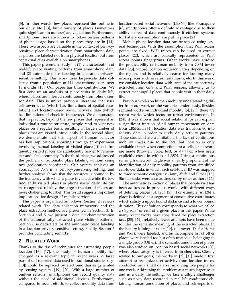
)Fig. 1. Cumulative distribution of users with respect to theaverage number of visits per day and the number of dis-tinct places visited during the data collection campaign.

and not sure. For the second question, “This location ishighly relevant to me.”, the user chose a score from 1(totally disagree) to 5 (totally agree). The third questionconcerns the visit frequency, “I visit this location ...”,where the user selected one among 6 options: Once a dayor more, 4-6 times per week, 1-2 times per week, 1-3 times permonth, Less than once a month, and Never. Finally, the userwas asked to select the most appropriate place label froma list of 22 mutually exclusive predefined labels. Besidesthe list of labels, there is a special category named ”Idon’t know” which was introduced for places that theuser could not remember or did not want to provideannotation for. In practice, 17% of the selected infrequentplaces were labeled as ”I don’t know” while only 3% ofthe selected top places were assigned the same label. Thetotal number of places annotated in this way was 912.

Demographic attributes. In order to study the de-pendencies between mobility patterns and demographicattributes, additional information about the user such asage or gender was also collected. Each user filled in aquestionnaire regarding demographic attributes. Besidesage and gender, users also declared their marital statusand their job position. There are three categories ofmarital status: single or divorced, in a relationship, andmarried or living with partner. Regarding job, there werefour categories in increasing order of position: Training(e.g., university student, apprentice, trainee), PhD stu-dent, Non-executive Employee, and Executive Employee.4 PLACE VISITING PATTERNS

Our analysis starts with basic statistics of places andtheir dynamics. We address the following questions:How many places do people go to in everyday life?How often are these places visited? How often do peoplevisit new places? What are the effects of demographicsand calendar in the dynamics of place visits? Each keyfinding is highlighted below in bold italic font.

How many places do people visit? Figure 1(left) illus-trates the cumulative distribution of users with respectto the average number of visits per day, showing thata large fraction of people visited from 2 to 4 placesper day. Note that the typical home-work-home dailyroutine corresponds to 2 visits per day since we onlycount the check-in time of visits: one at Work in themorning, and one at Home in the evening. Compared

1 2 3 4 5 10 20 50 100 200 500 100050

60

70

80

90

100

total number of visits during campaign (logscale)

pe

rce

nta

ge

of

pla

ce

s (

%)

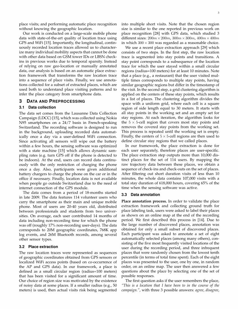
Fig. 2. Cumulative distribution of places with respect tothe total number of visits. The inset shows the probabilityfunction on log-log scale.

to previous studies on human dynamics, our data ismore complete and seems to reasonably reflect actualuser mobility trends. For example, the foursquare data in[32] is highly sparse, with one checkin every five days onaverage, while in [5], [23], location data is only availablewhen people make calls or send SMS .

We estimated that, on average, each person visited 90distinct places during the data collection campaign. Toget clearer understanding on the variation among peo-ple, Figure 1(right) shows the cumulative distributionof users with respect to the number of distinct placesvisited during the study. Most people visited 50-150places, furthermore there are 8% of users who visitedmore that 150 places, and 16% of users visited lessthan 50 places during the recording period. We remarkthat the recording time varies from 4 to 18 monthsdepending on the user, so the results presented here areinfluenced by that fact. More reliable measures related tothe number of places people visited will be consideredlater in the section.

How often are places visited? While people can easilyprovide a list of frequently visited places in their lives,it would be hard to exactly recall the list of placesvisited only a few times, even for those that correspondto valuable experiences. Studying the set of places thatpeople visited during one year and a half, we found asimple explanation to this observation: there are a hugenumber of infrequently visited places compared to afew places places that people usually go. In Figure 2,we show the cumulative distributions of the number ofplaces with respect to visit frequency. Note that the linearshape of the log-log plot in the inset of Figure 2 suggeststhat the distribution follows the Zipf’s law, which ispopular for distributions of frequency over rank. Onehalf of the places were visited only once during thecampaign, and the fraction of places that were visitedmore than once a month is less than 10%, while onlyabout 3% of places were visited at least once a week. Thisalso means that over the set of places that people visitedfor at least 10 minutes, the largest fraction correspondsto places that were only occasionally visited.

At what rate do people visit new places? To studyhow often people visit new places, we computed thenumber of distinct places in each week and the number

5

2 4 6 8 10 12 14 16

1

2

3

416−21 year olds

22−27 year olds

28−32 year olds

33−38 year olds

39−44 year olds

45+

#distinct places per week

#n

ew

pla

ce

s p

er

we

ek

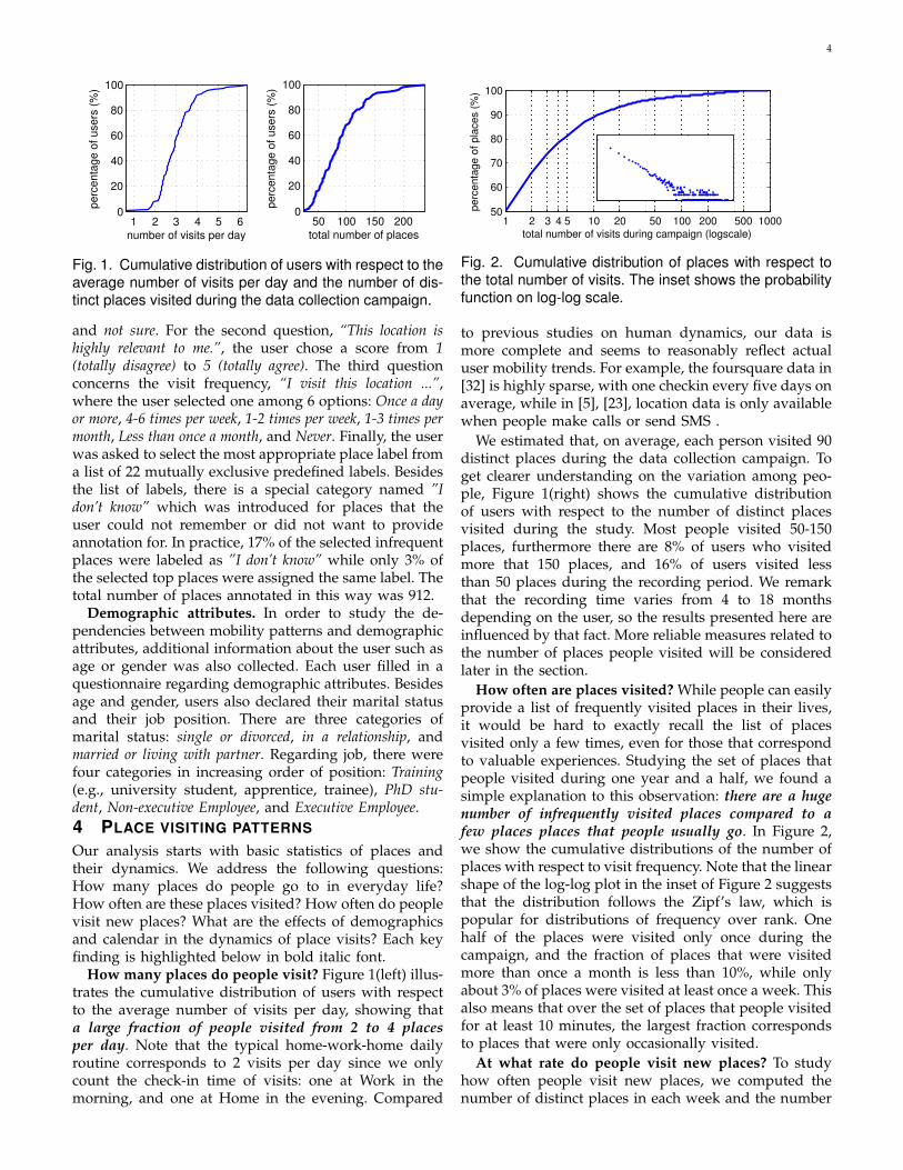
Fig. 3. Number of distinct places visited per week vs.number of new places visited per week for each partici-pant. Marker represents age group.

TABLE 1Average weekly number of visits, average weekly

number of distinct visited places, and average weeklynumber of new visited places for each group of people.

Standard deviations are also reported.Gender #visits #distinct #new

Female 19.9±5.0 7.5±1.9 1.7±0.7Male 22.0±6.5 7.5±2.4 1.7±0.8

Marital status #visits #distinct #newSingle or Divorce 21.2±7.1 7.3±2.4 1.6±0.7In a relationship 22.9±6.5 8.8±2.4 2.1±1.0Married or living with partner 19.8±4.3 6.8±1.6 1.5±0.6

Job #visits #distinct #newTraining 19.7±7.6 7.2±2.5 1.5±0.5PhD student 21.8±5.7 7.4±2.0 1.6±0.7Non-executive Employee 20.7±5.3 7.5±2.1 1.7±0.8Executive Employee 22.2±7.8 7.8±3.1 1.9±1.0

of new places that were discovered in that week (i.e.,places that had not been visited since the data collectionstarted). Then, the average values over active weeks(i.e., weeks with location data) were used as two basicmobility features for each user. As can be seen in Figure3, the average value across users for the first feature(horizontal axis) is roughly 7.5. Among the set of distinctplaces in a week, a few (1.7±0.8) of them are new places,while others are probably frequently visited places suchas home, work, or a favorite coffee shop. Note that theage group does not influence much these two mobilityfeatures as the distribution are mixed. There is a strongcorrelation (ρ = 0.744, p < 10−20) between the number ofdistinct places per week and the number of new placesper week. In other words, people who visit many placesa week also regularly visit many new places. Moreover,while the number of new places per week generallydecreases over time, we found that for some users, thenumber of places keeps increasing linearly until the endof the recording period (up to 79 weeks). Compared toa previous study [33] which suggests that the numberof distinct places at time t follows S(t) = tµ whereµ = 0.6±0.02 indicates a slow-down at large time scales,our results show that the value of µ varies depending onthe person: human location traces are not created equaland some people keep visiting new places on a regularbasis (i.e., µ = 1), at least for the 18-month scale.

Do demographics affect place visiting patterns? Wecontinue the analysis by studying the dependencies

between the mobility statistics and some demographicattributes (see Table 1). Interestingly, we observe nodifference between male and female in the number ofdistinct places per week and the number of new placesper week. However, men are slightly more mobile thanwomen if we look at the average number of visits perweek (first column in Table 1). In order to judge if thedifference is statistically significant, we use the Tukey-Kramer method together with ANOVA, in which twoestimates of mean value being compared are signifi-cantly different if their Tukey confidence intervals aredisjoint. The post-hoc testing of ANOVA shows thatthe difference between male and female in the averagenumber of visits per week is statistically significant with90% confidence intervals. Among the set of studieddemographic attributes, marital status was found tohave the strongest relation to mobility features. Whileprevious studies based on self-reported data showsthat there is a difference in mobility patterns betweenmarried and unmarried people [34], [35], we foundthat the difference between married people and peoplewho are in a relationship is even more significant. InTable 1, people who declared to be in a relationshiphave the highest mean values for the three reportedstatistics, and people who were married or living withtheir partner have the lowest values. Using the samepost-hoc testing of ANOVA, we found that the numberof distinct places and the number of new places aresignificantly different between the group of people inrelationships and the other two. For the average numberof visits per week, only the difference between the groupof people in relationships and the group of marriedpeople is statistically significant. Finally, we observe thatthe higher job position people have, the higher averagenumber of distinct places they visit. Note however thatthe difference is relatively low compared to the variancein each job group. Statistical tests on this data did notreturn any significant difference.

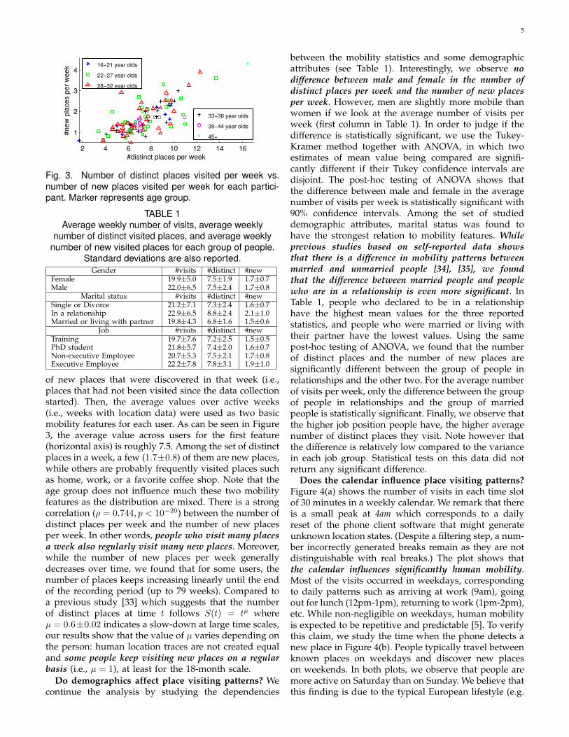
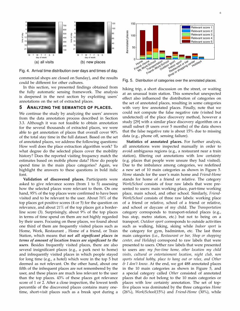
Does the calendar influence place visiting patterns?Figure 4(a) shows the number of visits in each time slotof 30 minutes in a weekly calendar. We remark that thereis a small peak at 4am which corresponds to a dailyreset of the phone client software that might generateunknown location states. (Despite a filtering step, a num-ber incorrectly generated breaks remain as they are notdistinguishable with real breaks.) The plot shows thatthe calendar influences significantly human mobility.Most of the visits occurred in weekdays, correspondingto daily patterns such as arriving at work (9am), goingout for lunch (12pm-1pm), returning to work (1pm-2pm),etc. While non-negligible on weekdays, human mobilityis expected to be repetitive and predictable [5]. To verifythis claim, we study the time when the phone detects anew place in Figure 4(b). People typically travel betweenknown places on weekdays and discover new placeson weekends. In both plots, we observe that people aremore active on Saturday than on Sunday. We believe thatthis finding is due to the typical European lifestyle (e.g.

6

day of week

tim

e o

f day

M T W T F S S

0

3

6

9

12

15

18

21100

200

300

400

500

600

700

(a) all visitsday of week

tim

e o

f day

M T W T F S S

0

3

6

9

12

15

18

21 20

40

60

80

100

120

(b) new places

Fig. 4. Arrival time distribution over days and times of day.

commercial shops are closed on Sunday), and the resultscould be different for other cultures.

In this section, we presented findings obtained fromthe fully automatic sensing framework. The analysisis deepened in the next section by exploiting users’annotations on the set of extracted places.

5 ANALYZING THE SEMANTICS OF PLACES.We continue the study by analyzing the users’ answersfrom the data annotation process described in Section3.3. Although it was not feasible to obtain annotationfor the several thousands of extracted places, we wereable to get annotation of places that overall cover 90%of the total stay time in the full dataset. Based on the setof annotated places, we address the following questions:How well does the place extraction algorithm work? Towhat degree do the selected places cover the mobilityhistory? Does the reported visiting frequency match theestimates based on mobile phone data? How do peoplespend time in the main place categories? Again, wehighlight the answers to these questions in bold italicfont.

Validation of discovered places. Participants wereasked to give relevance scores (from 1 to 5) assessinghow the selected places were relevant to them. On onehand, 95% of the top places were confirmed to have beenvisited and to be relevant to the user. About 70% of thetop places got positive scores (4 or 5) for the question onrelevance, and about 21% of the top places got a border-line score (3). Surprisingly, about 9% of the top placesin terms of time spend on them are not highly regardedby their users. Focusing on these places, we found aboutone third of them are frequently visited places such asHome, Work, Restaurant , Home of a friend, or TrainStation, which means that not all significant places interms of amount of location traces are significant to theusers. Besides frequently visited places, there are alsoseveral insignificant places (e.g., a park next to home)and infrequently visited places in which people stayedfor long time (e.g., a hotel) which were in the top 5 butdeemed as not relevant. On the other hand, about onefifth of the infrequent places are not remembered by theuser, and these places are much less relevant to the userthan the top places. 43% of these places got relevancescore of 1 or 2. After a close inspection, the lowest tenthpercentile of the discovered places contains many one-time, short-visit places such as a break spot during a

0

50

100

150

Home

Friend−

Home

My Work/School

Transportatio

n

Friend−

Work/School

Outdoor sport

Indoor sport

Restaurant or b

ar

Shop or shopping center

Holidays

#a

nn

ota

ted

pla

ce

s

Relevant score 1

Relevant score 2

Relevant score 3

Relevant score 4

Relevant score 5

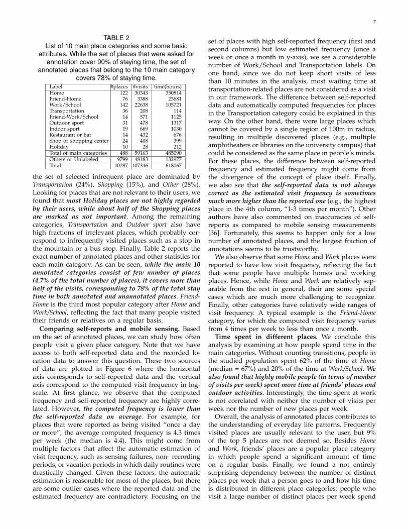
Fig. 5. Distribution of categories over the annotated places.

hiking trip, a short discussion on the street, or waitingat an unusual train station. This somewhat unexpectedeffect also influenced the distribution of categories onthe set of annotated places, resulting in some categorieswith very few annotated places. Finally, note that wecould not compute the false negative rate (visited butundetected) of the place discovery method, however astudy [29] with a similar place discovery algorithm on asmall subset (8 users over 5 months) of the data showsthat the false negative rate is about 15% due to missingdata (e.g., phone off, sensing failure).

Statistics of annotated places. For further analysis,all annotations were inspected manually in order toavoid ambiguous regions (e.g., a restaurant near a trainstation), filtering out annotations with low certainty(e.g. places that people were unsure they had visited).Due to the imbalance among categories, we redefineda new set of 10 main categories as shown in Figure 5.Home stands for the user’s main home and Friend-Homestands for home of a friend or relative. The categoryWork/School consists of four raw labels that were pre-sented to users: main working place, part-time workingplace, main school, and other school. Similarly, Friend-Work/School consists of three raw labels: working placeof a friend or relative, school of a friend or relative,and school or daycare of my child. The Transportationcategory corresponds to transport-related places (e.g.,bus stop, metro station, etc.) but not to being on atransport. Outdoor sport corresponds to outside activitiessuch as walking, hiking, skiing while Indoor sport isthe category for gym, badminton, etc. The last threemain categories (i.e., Restaurant or bar, Shop or shoppingcenter, and Holiday) correspond to raw labels that werepresented to users. Other raw labels that were presentedto users are: my free-time home, other location my childvisits, cultural or entertainment location, night club, nonsports related hobby, place to hang out or relax, and Other& I don’t know. At the end, we got 488 annotated placesin the 10 main categories as shown in Figure 5, anda special category called Other consisted of annotatedplaces that do not belong to the 10 main categories orplaces with low certainty annotation. The set of top-five places was dominated by the three categories Home(26%), Work/School(15%) and Friend-Home (30%), while

7

TABLE 2List of 10 main place categories and some basic

attributes. While the set of places that were asked forannotation cover 90% of staying time, the set of

annotated places that belong to the 10 main categorycovers 78% of staying time.

Label #places #visits time(hours)Home 122 30343 350814Friend-Home 76 3388 23681Work/School 142 22638 105721Transportation 36 208 114Friend-Work/School 14 571 1125Outdoor sport 31 478 1317Indoor sport 19 669 1030Restaurant or bar 14 432 676Shop or shopping center 24 408 399Holiday 10 28 212Total of main categories 488 59163 485090Others or Unlabeled 9799 48183 132977Total 10287 107346 618067

the set of selected infrequent place are dominated byTransportation (24%), Shopping (15%), and Other (28%).Looking for places that are not relevant to their users, wefound that most Holiday places are not highly regardedby their users, while about half of the Shopping placesare marked as not important. Among the remainingcategories, Transportation and Outdoor sport also havehigh fractions of irrelevant places, which probably cor-respond to infrequently visited places such as a stop inthe mountain or a bus stop. Finally, Table 2 reports theexact number of annotated places and other statistics foreach main category. As can be seen, while the main 10annotated categories consist of few number of places(4.7% of the total number of places), it covers more thanhalf of the visits, corresponding to 78% of the total staytime in both annotated and unannotated places. Friend-Home is the third most popular category after Home andWork/School, reflecting the fact that many people visitedtheir friends or relatives on a regular basis.

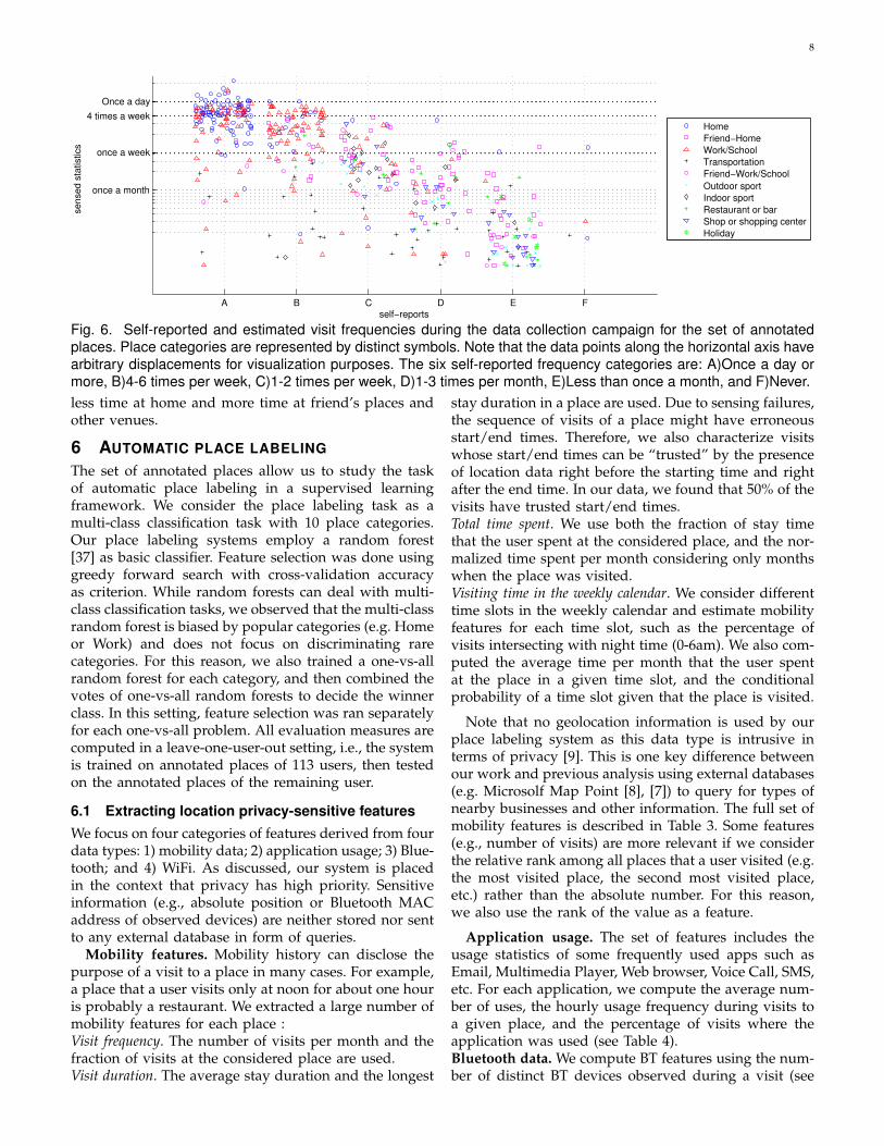
Comparing self-reports and mobile sensing. Basedon the set of annotated places, we can study how oftenpeople visit a given place category. Note that we haveaccess to both self-reported data and the recorded lo-cation data to answer this question. These two sourcesof data are plotted in Figure 6 where the horizontalaxis corresponds to self-reported data and the verticalaxis correspond to the computed visit frequency in log-scale. At first glance, we observe that the computedfrequency and self-reported frequency are highly corre-lated. However, the computed frequency is lower thanthe self-reported data on average. For example, forplaces that were reported as being visited “once a dayor more”, the average computed frequency is 4.3 timesper week (the median is 4.4). This might come frommultiple factors that affect the automatic estimation ofvisit frequency, such as sensing failures, non- recordingperiods, or vacation periods in which daily routines weredrastically changed. Given these factors, the automaticestimation is reasonable for most of the places, but thereare some outlier cases where the reported data and theestimated frequency are contradictory. Focusing on the

set of places with high self-reported frequency (first andsecond columns) but low estimated frequency (once aweek or once a month in y-axis), we see a considerablenumber of Work/School and Transportation labels. Onone hand, since we do not keep short visits of lessthan 10 minutes in the analysis, most waiting time attransportation-related places are not considered as a visitin our framework. The difference between self-reporteddata and automatically computed frequencies for placesin the Transportation category could be explained in thisway. On the other hand, there were large places whichcannot be covered by a single region of 100m in radius,resulting in multiple discovered places (e.g., multipleamphitheaters or libraries on the university campus) thatcould be considered as the same place in people’s minds.For these places, the difference between self-reportedfrequency and estimated frequency might come fromthe divergence of the concept of place itself. Finally,we also see that the self-reported data is not alwayscorrect as the estimated visit frequency is sometimesmuch more higher than the reported one (e.g., the highestplace in the 4th column, “1-3 times per month”). Otherauthors have also commented on inaccuracies of self-reports as compared to mobile sensing measurements[36]. Fortunately, this seems to happen only for a lownumber of annotated places, and the largest fraction ofannotations seems to be trustworthy.

We also observe that some Home and Work places werereported to have low visit frequency, reflecting the factthat some people have multiple homes and workingplaces. Hence, while Home and Work are relatively sep-arable from the rest in general, their are some specialcases which are much more challenging to recognize.Finally, other categories have relatively wide ranges ofvisit frequency. A typical example is the Friend-Homecategory, for which the computed visit frequency variesfrom 4 times per week to less than once a month.

Time spent in different places. We conclude thisanalysis by examining at how people spend time in themain categories. Without counting transitions, people inthe studied population spent 62% of the time at Home(median = 67%) and 20% of the time at Work/School. Wealso found that highly mobile people (in terms of numberof visits per week) spent more time at friends’ places andoutdoor activities. Interestingly, the time spent at workis not correlated with neither the number of visits perweek nor the number of new places per week.

Overall, the analysis of annotated places contributes tothe understanding of everyday life patterns. Frequentlyvisited places are usually relevant to the user, but 9%of the top 5 places are not deemed so. Besides Homeand Work, friends’ places are a popular place categoryin which people spend a significant amount of timeon a regular basis. Finally, we found a not entirelysurprising dependency between the number of distinctplaces per week that a person goes to and how his timeis distributed in different place categories: people whovisit a large number of distinct places per week spend

8

A B C D E F

once a month

once a week

4 times a week

Once a day

self−reports

se

nse

d s

tatistics

Home

Friend−Home

Work/School

Transportation

Friend−Work/School

Outdoor sport

Indoor sport

Restaurant or bar

Shop or shopping center

Holiday

Fig. 6. Self-reported and estimated visit frequencies during the data collection campaign for the set of annotatedplaces. Place categories are represented by distinct symbols. Note that the data points along the horizontal axis havearbitrary displacements for visualization purposes. The six self-reported frequency categories are: A)Once a day ormore, B)4-6 times per week, C)1-2 times per week, D)1-3 times per month, E)Less than once a month, and F)Never.less time at home and more time at friend’s places andother venues.

6 AUTOMATIC PLACE LABELING

The set of annotated places allow us to study the taskof automatic place labeling in a supervised learningframework. We consider the place labeling task as amulti-class classification task with 10 place categories.Our place labeling systems employ a random forest[37] as basic classifier. Feature selection was done usinggreedy forward search with cross-validation accuracyas criterion. While random forests can deal with multi-class classification tasks, we observed that the multi-classrandom forest is biased by popular categories (e.g. Homeor Work) and does not focus on discriminating rarecategories. For this reason, we also trained a one-vs-allrandom forest for each category, and then combined thevotes of one-vs-all random forests to decide the winnerclass. In this setting, feature selection was ran separatelyfor each one-vs-all problem. All evaluation measures arecomputed in a leave-one-user-out setting, i.e., the systemis trained on annotated places of 113 users, then testedon the annotated places of the remaining user.

6.1 Extracting location privacy-sensitive featuresWe focus on four categories of features derived from fourdata types: 1) mobility data; 2) application usage; 3) Blue-tooth; and 4) WiFi. As discussed, our system is placedin the context that privacy has high priority. Sensitiveinformation (e.g., absolute position or Bluetooth MACaddress of observed devices) are neither stored nor sentto any external database in form of queries.

Mobility features. Mobility history can disclose thepurpose of a visit to a place in many cases. For example,a place that a user visits only at noon for about one houris probably a restaurant. We extracted a large number ofmobility features for each place :Visit frequency. The number of visits per month and thefraction of visits at the considered place are used.Visit duration. The average stay duration and the longest

stay duration in a place are used. Due to sensing failures,the sequence of visits of a place might have erroneousstart/end times. Therefore, we also characterize visitswhose start/end times can be “trusted” by the presenceof location data right before the starting time and rightafter the end time. In our data, we found that 50% of thevisits have trusted start/end times.Total time spent. We use both the fraction of stay timethat the user spent at the considered place, and the nor-malized time spent per month considering only monthswhen the place was visited.Visiting time in the weekly calendar. We consider differenttime slots in the weekly calendar and estimate mobilityfeatures for each time slot, such as the percentage ofvisits intersecting with night time (0-6am). We also com-puted the average time per month that the user spentat the place in a given time slot, and the conditionalprobability of a time slot given that the place is visited.

Note that no geolocation information is used by ourplace labeling system as this data type is intrusive interms of privacy [9]. This is one key difference betweenour work and previous analysis using external databases(e.g. Microsolf Map Point [8], [7]) to query for types ofnearby businesses and other information. The full set ofmobility features is described in Table 3. Some features(e.g., number of visits) are more relevant if we considerthe relative rank among all places that a user visited (e.g.the most visited place, the second most visited place,etc.) rather than the absolute number. For this reason,we also use the rank of the value as a feature.

Application usage. The set of features includes theusage statistics of some frequently used apps such asEmail, Multimedia Player, Web browser, Voice Call, SMS,etc. For each application, we compute the average num-ber of uses, the hourly usage frequency during visits toa given place, and the percentage of visits where theapplication was used (see Table 4).Bluetooth data. We compute BT features using the num-ber of distinct BT devices observed during a visit (see

9

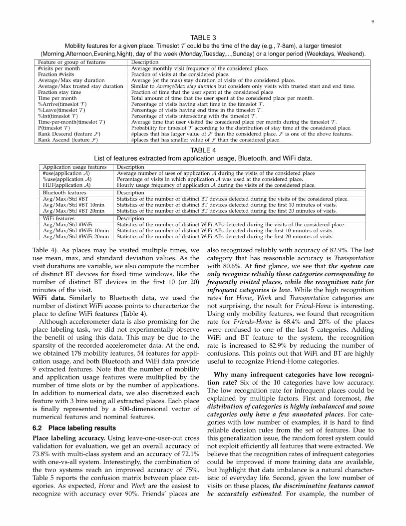
TABLE 3Mobility features for a given place. Timeslot T could be the time of the day (e.g., 7-8am), a larger timeslot

(Morning,Afternoon,Evening,Night), day of the week (Monday,Tuesday,...,Sunday) or a longer period (Weekdays, Weekend).Feature or group of features Description#visits per month Average monthly visit frequency of the considered place.Fraction #visits Fraction of visits at the considered place.Average/Max stay duration Average (or the max) stay duration of visits of the considered place.Average/Max trusted stay duration Similar to Average/Max stay duration but considers only visits with trusted start and end time.Fraction stay time Fraction of time that the user spent at the considered placeTime per month Total amount of time that the user spent at the considered place per month.%Arrive(timeslot T ) Percentage of visits having start time in the timeslot T .%Leave(timeslot T ) Percentage of visits having end time in the timeslot T .%Int(timeslot T ) Percentage of visits intersecting with the timeslot T .Time-per-month(timeslot T ) Average time that user visited the considered place per month during the timeslot T .P(timeslot T ) Probability for timeslot T according to the distribution of stay time at the considered place.Rank Descend (feature F ) #places that has larger value of F than the considered place. F is one of the above features.Rank Ascend (feature F ) #places that has smaller value of F than the considered place.

TABLE 4List of features extracted from application usage, Bluetooth, and WiFi data.

Application usage features Description#use(application A) Average number of uses of application A during the visits of the considered place%use(application A) Percentage of visits in which application A was used at the considered place.HUF(application A) Hourly usage frequency of application A during the visits of the considered place.Bluetooth features DescriptionAvg/Max/Std #BT Statistics of the number of distinct BT devices detected during the visits of the considered place.Avg/Max/Std #BT 10min Statistics of the number of distinct BT devices detected during the first 10 minutes of visits.Avg/Max/Std #BT 20min Statistics of the number of distinct BT devices detected during the first 20 minutes of visits.WiFi features DescriptionAvg/Max/Std #WiFi Statistics of the number of distinct WiFi APs detected during the visits of the considered place.Avg/Max/Std #WiFi 10min Statistics of the number of distinct WiFi APs detected during the first 10 minutes of visits.Avg/Max/Std #WiFi 20min Statistics of the number of distinct WiFi APs detected during the first 20 minutes of visits.

Table 4). As places may be visited multiple times, weuse mean, max, and standard deviation values. As thevisit durations are variable, we also compute the numberof distinct BT devices for fixed time windows, like thenumber of distinct BT devices in the first 10 (or 20)minutes of the visit.WiFi data. Similarly to Bluetooth data, we used thenumber of distinct WiFi access points to characterize theplace to define WiFi features (Table 4).

Although accelerometer data is also promising for theplace labeling task, we did not experimentally observethe benefit of using this data. This may be due to thesparsity of the recorded accelerometer data. At the end,we obtained 178 mobility features, 54 features for appli-cation usage, and both Bluetooth and WiFi data provide9 extracted features. Note that the number of mobilityand application usage features were multiplied by thenumber of time slots or by the number of applications.In addition to numerical data, we also discretized eachfeature with 3 bins using all extracted places. Each placeis finally represented by a 500-dimensional vector ofnumerical features and nominal features.

6.2 Place labeling resultsPlace labeling accuracy. Using leave-one-user-out crossvalidation for evaluation, we get an overall accuracy of73.8% with multi-class system and an accuracy of 72.1%with one-vs-all system. Interestingly, the combination ofthe two systems reach an improved accuracy of 75%.Table 5 reports the confusion matrix between place cat-egories. As expected, Home and Work are the easiest torecognize with accuracy over 90%. Friends’ places are

also recognized reliably with accuracy of 82.9%. The lastcategory that has reasonable accuracy is Transportationwith 80.6%. At first glance, we see that the system canonly recognize reliably these categories corresponding tofrequently visited places, while the recognition rate forinfrequent categories is low. While the high recognitionrates for Home, Work and Transportation categories arenot surprising, the result for Friend-Home is interesting.Using only mobility features, we found that recognitionrate for Friends-Home is 68.4% and 20% of the placeswere confused to one of the last 5 categories. AddingWiFi and BT feature to the system, the recognitionrate is increased to 82.9% by reducing the number ofconfusions. This points out that WiFi and BT are highlyuseful to recognize Friend-Home categories.

Why many infrequent categories have low recogni-tion rate? Six of the 10 categories have low accuracy.The low recognition rate for infrequent places could beexplained by multiple factors. First and foremost, thedistribution of categories is highly imbalanced and somecategories only have a few annotated places. For cate-gories with low number of examples, it is hard to findreliable decision rules from the set of features. Due tothis generalization issue, the random forest system couldnot exploit efficiently all features that were extracted. Webelieve that the recognition rates of infrequent categoriescould be improved if more training data are available,but highlight that data imbalance is a natural character-istic of everyday life. Second, given the low number ofvisits on these places, the discriminative features cannotbe accurately estimated. For example, the number of

10

TABLE 5Confusion matrix of the place labeling task and accuracy(%TP) for each category. Rows represent the true label

and columns represent the predicted label. False Positive(%FP) rates are reported.

H FH W/S T FW O I R S Hld %TP %FPHome 112 7 2 1 0 0 0 0 0 0 91.8 2.5Friend-Home 5 63 3 3 0 0 0 1 1 0 82.9 6.1Work/School 3 5 128 2 1 1 0 0 1 1 90.1 9.0Transportation 0 2 3 29 0 0 0 0 1 1 80.6 4.9Friend-Work/School 0 2 7 2 1 0 1 0 1 0 7.1 0.2Outdoor sport 1 3 4 2 0 12 3 0 5 1 38.7 2.4Indoor sport 0 1 5 0 0 6 5 1 1 0 26.3 0.9Restaurant or bar 0 1 5 3 0 0 0 3 1 1 21.4 0.6Shop or shopping center 0 1 2 7 0 3 0 1 10 0 41.7 2.6Holiday 0 3 0 2 0 1 0 0 1 3 30.0 0.8

TABLE 6Place labeling accuracy with different feature sets.

Feature sets Acc (%) Feature sets Acc (%)(M)obility 70.3(W)iFi 50.4 M+W 71.7(B)T 51.0 M+W+B 74.6(A)PP 48.0 M+W+B+A 75.0

Bluetooth devices at a given place could significantlychange over time. If the place is visited just once or twice,then the estimation of the feature Avg #BT (averagenumber of BT devices) could be inaccurate. Intuitively,the more frequently a place is visited, the more informa-tion there is about the place for making any prediction.Finally, one could expect that in some cases, the placecategory cannot be recognized from location privacy-sensitive features. For example, the Friend-Work categoryis highly confused with Work/School, Friend-Home, oreven Transportation, which are much more popular interms of number of annotated samples. Despite the lowrecognition rate, we also see promising results for somecategories such as Outdoor sport, Shop or Shopping center,or Holiday. One could expect that with more data anddata types, the recognition rate would be improved.

How does each data type improve accuracy? Finally,we study how each feature set contributes to the finalaccuracy. Table 6 reports the accuracy with differentfeature subsets. As can be seen, reasonable accuracy canbe achieved with mobility features only. We found thatthe most important mobility features are the visiting timeof a given place (e.g., the percentage of visits intersectingwith the timeslot 5-6am, or the fraction of departurefor the timeslot 8-9pm), the fraction of time spent atthe place, and the amount of time spent on weekendsper month. The use of each of the 3 remaining featuresets separately results in modest performance. However,WiFi and Bluetooth features are relatively useful for thefinal system as they improve the accuracy by about 4%.WiFi contributes 2 features to the system: the averagenumber of APs for the first 20 minutes, and the maxi-mum number of APs observed during a single visit ofthe place. For the statistics on Bluetooth data, we foundthat the maximum number and the standard deviationof BT devices during the first 20 minutes are the mostimportant features, which suggests that the BT statisticson 20-minute intervals is more robust than the one with10-minute intervals or with the total stay time. Finally,

the accuracy with only APP features is about 48.0%, withthe most important applications (in descending order)being Clock, Profiles, Search, Telephone, Web, Maps.However, the contribution of application usage featuresto the final system is relatively low, which may due to thelow level of usage of applications on the Nokia N95 [14].As phone app usage is much more active for modernsmartphones, application usage features should still bepromising for place labeling.

7 FINAL DISCUSSION AND IMPLICATIONS

This study contributes to our understanding of placesin people’s daily lives and to the possibility of inferringplace categories from smartphone data.

Our analysis is based on the LDCC mobile sensingframework that extracts automatically places that peo-ple visit. While people usually follow simple routinesinvolving a few frequent places, we observe that mostof them keep exploring new places, resulting in a largenumber of places for many individuals. If people couldreceive relevant recommendation for new places (e.g.,restaurants, leisure-related places, etc.), the number ofvisited places could be even higher. The study suggeststhat personalized recommendation could be a plausibleapproach. For instance, the number of distinct placesper week has significant correlation with other variablessuch as the frequency at which people visit new places,and this might suggest what users might find suchservice useful.

Together with annotation, we also used feedback onthe meaning and the quality of some of the discoveredplaces (5 top frequent places and 3 infrequent places).Highly positive feedback was obtained for the set offrequent places, with 95% of them confirmed by theusers. Interestingly, one fifth of the set of infrequentplaces were not remembered by people. While some ofthese places might actually not be important for users,we believe that if the phone was able to remind the userabout events that might have been forgotten, they couldelicit positive personal uses related to memory and self-reflection.

Along with this analysis on place labeling, the pre-diction task was proposed as part of the Mobile DataChallenge [38]. Our results in this paper show thatit is not easy to recognize the semantic meaning fora large number of places in our lives if the actualphysical location is not known. Frequently visited placessuch as home, work or the home of a friend can bereliably recognized using only location-sensitive smart-phone data. As people spend most time in these frequentplaces, the place category can be recognized accurately.However, the recognition rate for infrequent places isrelative low due to many factors including the currentprivacy-sensitive data we use. This is a valuable resultif privacy is the main concern (i.e., if users wanted thatthe category of certain infrequent places could not beinferred automatically).

11

If the category of infrequent places is not a privacyconcern, one could think of adding more sensors to thesmartphone in order to improve the recognition rate ofinfrequent places, besides collecting more training data.For example, a light sensor and a thermometer couldhelp recognizing indoor-outdoor environments with-out heavy battery consumption. Acoustic noise sensorscould be a privacy-sensitive solution for adding audiodata. We remark that while the absolute recognition rateis low for many infrequent categories, the results arestill promising and our current system could be usefuleven for complex situations. For example, in the caseof confusion among a few categories, the system couldpresent the most likely categories to the user asking forannotation. This could be a reasonable solution if therequired amount of interaction was minimal and therewere clear incentives for users to tag their own data. Thisdirection might be investigated in the future.

ACKNOWLEDGMENTS

This work was funded by Nokia Research Center Lau-sanne (NRC) through the LS-CONTEXT project. Wethank Jan Blom (Nokia Research) for sharing the usersurveys, Juha Laurila (Nokia Research) for discussions,and Olivier Bornet (Idiap) for technical support.REFERENCES[1] L. Barkhuus, B. Brown, M. Bell, S. Sherwood, M. Hall, and

M. Chalmers, “From awareness to repartee: sharing locationwithin social groups,” in Proc. CHI ’08, 2008, pp. 497–506.

[2] H. Cramer, M. Rost, and L. E. Holmquist, “Performing a check-in: emerging practices, norms and ’conflicts’ in location-sharingusing foursquare,” in Proc. MobileHCI ’11. New York, NY, USA:ACM, 2011, pp. 57–66.

[3] J. Hightower, S. Consolvo, A. LaMarca, I. Smith, and J. Hughes,“Learning and recognizing the places we go,” in UbiComp 2005:Ubiquitous Computing, ser. Lecture Notes in Computer Science,M. Beigl, S. Intille, J. Rekimoto, and H. Tokuda, Eds. SpringerBerlin / Heidelberg, 2005, vol. 3660, pp. 159–176.

[4] S. Phithakkitnukoon, T. Horanont, G. Di Lorenzo, R. Shibasaki,and C. Ratti, “Activity-aware map: identifying human daily ac-tivity pattern using mobile phone data,” in Proc. of the 1st Int.Conf. on Human behavior understanding, 2010, pp. 14–25.

[5] M. C. Gonzalez, C. A. Hidalgo, and A.-L. Barabasi, “Understand-ing individual human mobility patterns,” Nature, vol. 453, no.7196, pp. 779–782, June 2008.

[6] A. Noulas, S. Scellato, R. Lambiotte, M. Pontil, and C. Mascolo, “Atale of many cities: universal patterns in human urban mobility,”PloS one, vol. 7, no. 5, p. e37027, 2012.

[7] L. Liao, D. Fox, and H. Kautz, “Location-based activity recogni-tion using relational markov networks,” in Proc. IJCAI ’05, 2005,pp. 773–778.

[8] R. Hariharan, J. Krumm, and E. Horvitz, “Web-enhanced gps,” inInternational Workshop on Locationand Context-Awareness. Springer,2005, pp. 95–104.

[9] K. P. Tang, P. Keyani, J. Fogarty, and J. I. Hong, “Putting peoplein their place: an anonymous and privacy-sensitive approach tocollecting sensed data in location-based applications,” in Proc. CHI’06. ACM, 2006, pp. 93–102.

[10] J. Krumm, “A survey of computational location privacy,” PersonalUbiquitous Computing, vol. 13, pp. 391–399, August 2009.

[11] ——, “Inference attacks on location tracks,” in Proc. Pervasive’07.Berlin, Heidelberg: Springer-Verlag, 2007, pp. 127–143.

[12] M. Duckham and L. Kulik, “Location privacy and location-awarecomputing,” Dynamic & mobile GIS: investigating change in spaceand time, pp. 34–51, 2006.

[13] N. Eagle and A. Pentland, “Eigenbehaviors: identifying structurein routine,” Behavioral Ecology and Sociobiology, vol. 63, no. 7, pp.1057–1066, May 2009.

[14] T. M. T. Do, J. Blom, and D. Gatica-Perez, “Smartphone usage inthe wild: a large-scale analysis of applications and context,” inProc. ICMI ’11. New York, NY, USA: ACM, 2011, pp. 353–360.

[15] N. Kiukkonen, J. Blom, O. Dousse, D. Gatica-Perez, and J. Laurila,“Towards rich mobile phone datasets: Lausanne data collectioncampaign,” in Proc. ICPS, Berlin, 2010.

[16] T. Liu, P. Bahl, and I. Chlamtac, “Mobility modeling, locationtracking, and trajectory prediction in wireless ATM networks,”Selected Areas in Communications, vol. 16, no. 6, pp. 922–936, 1998.

[17] R. Bajaj, S. L. Ranaweera, and D. P. Agrawal, “GPS: location-tracking technology,” Computer, vol. 35, no. 4, pp. 92–94, 2002.

[18] J. Krumm and A. J. B. Brush, “Learning time-based presenceprobabilities.” in Proc. Pervasive’11, 2011, pp. 79–96.

[19] N. Eagle and A. (Sandy) Pentland, “Reality mining: sensingcomplex social systems,” Personal Ubiquitous Comput., vol. 10,no. 4, pp. 255–268, 2006.

[20] M. Raento, A. Oulasvirta, R. Petit, and H. Toivonen, “Context-phone: A prototyping platform for context-aware mobile applica-tions,” IEEE Pervasive Computing, vol. 4, no. 2, pp. 51–59, 2005.

[21] D. Kim, Y. Kim, D. Estrin, and M. Srivastava, “Sensloc: sensingeveryday places and paths using less energy,” in Proc. Sensys ’10.ACM, 2010, pp. 43–56.

[22] L. Vu, Q. Do, and K. Nahrstedt, “Jyotish: A novel frameworkfor constructing predictive model of people movement from jointwifi/bluetooth trace.” in PerCom’11, 2011, pp. 54–62.

[23] C. Song, Z. Qu, N. Blumm, and A.-L. Barabsi, “Limits of pre-dictability in human mobility,” Science, vol. 327, no. 5968, pp.1018–1021, 2010.

[24] E. Cho, S. A. Myers, and J. Leskovec, “Friendship and mobility:user movement in location-based social networks,” in Proc. KDD,2011, pp. 1082–1090.

[25] K. Farrahi and D. Gatica-Perez, “Probabilistic mining of socio-geographic routines from mobile phone data,” IEEE J-STSP, vol. 4,no. 4, pp. 746–755, 2010.

[26] J. H. Kang, W. Welbourne, B. Stewart, and G. Borriello, “Extractingplaces from traces of locations,” in Proc. WMASH 04. ACM Press,2004, pp. 110–118.

[27] M. Kim, D. Kotz, and S. Kim, “Extracting a mobility model fromreal user traces,” in Proc. INFOCOM ’06. Barcelona, Spain: IEEEComputer Society Press, April 2006.

[28] V. W. Zheng, Y. Zheng, X. Xie, and Q. Yang, “Collaborativelocation and activity recommendations with gps history data,”in Proc. WWW. ACM, 2010.

[29] R. Montoliu and D. Gatica-Perez, “Discovering human places ofinterest from multimodal mobile phone data,” in Proc. MUM,Limassol, Cyprus, 2010, pp. 12:1–12:10.

[30] M. Ye, D. Shou, W. Lee, P. Yin, and K. Janowicz, “On the semanticannotation of places in location-based social networks,” in Proc.KDD ’11. ACM, 2011, pp. 520–528.

[31] L. Liao, D. Fox, and H. Kautz, “Extracting places and activitiesfrom gps traces using hierarchical conditional random fields,” TheInternational Journal of Robotics Research, vol. 26, no. 1, pp. 119–134,2007.

[32] A. Noulas, S. Scellato, C. Mascolo, and M. Pontil, “An empiricalstudy of geographic user activity patterns in foursquare,” in Proc.ICWSM ’11, 2011, pp. 570–573.

[33] C. Song, T. Koren, P. Wang, and A. Barabasi, “Modelling thescaling properties of human mobility,” Nature Physics, vol. 6,no. 10, pp. 818–823, 2010.

[34] E. Pas, “The effect of selected sociodemographic characteristicson daily travel-activity behavior,” Environment and Planning A,vol. 16, no. 5, pp. 571–581, 1984.

[35] X. Lu and E. Pas, “Socio-demographics, activity participation andtravel behavior,” Transportation Research Part A: Policy and Practice,vol. 33, no. 1, pp. 1–18, 1999.

[36] N. Eagle, A. Pentland, and D. Lazer, “Inferring friendship net-work structure by using mobile phone data,” Proceedings of theNational Academy of Sciences, vol. 106, no. 36, pp. 15 274–15 278,2009.

[37] A. Liaw and M. Wiener, “Classification and regression by ran-domforest,” R news, vol. 2, no. 3, pp. 18–22, 2002.

[38] J. Laurila, D. Gatica-Perez, I. Aad, J. Blom, O. Bornet, T. Do,O. Dousse, J. Eberle, and M. Miettinen, “The mobile data chal-lenge: Big data for mobile computing research,” in Proc. MDCWorkshop, 2012.

12

Trinh Minh Tri Do received his PhD degreein Computer Science from Pierre and MarieCurie University, Paris, France in 2010. He isworking as a postdoctoral research at Idiap Re-search Institute, Switzerland. His research inter-ests include machine learning, optimization, pat-tern recognition, and ubiquitous computing. Hiscurrent work focuses on analyzing human andsocial behavior from large-scale mobile phonedata.

Daniel Gatica-Perez, S’01, M’02 received thePh.D. degree in Electrical Engineering from theUniversity of Washington, Seattle, in 2001. He isthe Head of the Social Computing Group at IdiapResearch Institute and Maitre d’Enseignementet de Recherche at the Swiss Federal Instituteof Technology in Lausanne (EPFL). His researchdevelops computational models, algorithms, andsystems for sensing and analysis of human andsocial behavior from sensor data. He has servedas Associate Editor of the IEEE Transactions on

Multimedia, Image and Vision Computing, Machine Vision and Applica-tions, and the Journal of Ambient Intelligence and Smart Environments.