The Physical Properties and Cosmic Environments of Quasars in the First Gyr of the Universe Chiara Mazzucchelli Max-Planck-Institut für Astronomie Heidelberg 2018

Welcome message from author
This document is posted to help you gain knowledge. Please leave a comment to let me know what you think about it! Share it to your friends and learn new things together.
Transcript

The Physical Propertiesand Cosmic Environments
of Quasars in the First Gyr of the Universe
Chiara Mazzucchelli
Max-Planck-Institut für Astronomie
Heidelberg 2018


Dissertation in Astronomysubmitted to the
Combined Faculties of the Natural Science and Mathematicsof the Ruperto-Carola-University of Heidelberg, Germany
for the degree ofDoctor of Natural Sciences
put forward by
Chiara Mazzucchelliborn in Gallarate, Italy
Oral examination: 12 July 2018


The Physical Propertiesand Cosmic Environments
of Quasars in the First Gyr of the Universe
Chiara Mazzucchelli
Max-Planck-Institut für Astronomie
Referees: Prof. Dr. Hans-Walter RixProf. Dr. Jochen Heidt


Abstract
Luminous quasars at redshift z &6, i.e. .1 Gyr after the Big Bang, are formidable probes ofthe early universe, at the edge of the Epoch of Reionization. These sources are predictedto be found in high–density peaks of the dark matter distribution at that time, surroundedby overdensities of galaxies. In this thesis, we present a search for and study of the mostdistant quasars, from the properties of their innermost regions, to those of their host galax-ies and of their Mpc–scale environments. We search for the highest redshift quasars in thePanoramic Survey Telescope and Rapid Response System 1 (Pan-STARRS1, PS1), discoveringsix new objects at z &6.5. Using optical/near–infrared spectroscopic data, we perform a homo-geneous analysis of the properties of 15 quasars at z& 6.5. In short : 1) The majority of z &6.5show large blueshifts of the broad CIV 1549 Å emission line, suggesting the presence of strongwinds/outflows; 2) They already host supermassive black holes (∼ 0.3− 5× 10⁹ M) in theircenters, which are accreting at a rate comparable to a luminosity–matched sample at z ∼1; 3)No evolution of the Fe II/Mg II abundance ratio with cosmic time is observed; 4) The sizes oftheir surrounding ionized bubbles weakly decrease with redshift. We present new millime-ter observations of the dust continuum and of the [CII] 158 µm emission line (one of the maincoolant of the intergalactic medium) in the host galaxies of four quasars, providing new accu-rate redshifts and [CII]/infrared luminosities. We study the Mpc–scale environment of a z ∼5.7quasar, via observations with broad– and narrow–band filters. We recover no overdensitiesof galaxies. Among the potential explanations for these findings, are that the ionizing radia-tion from the quasar prevents galaxy formation, the sources in the fields are dust–obscured,or quasars do not live in the most massive dark matter halos. Finally, we report sensitiveoptical/near–infrared follow–up observations of gas–rich companion galaxies to four quasarsat z &6, firstly detected with the Atacama Large Millimeter Array (ALMA). With the exceptionof one source, we detect no emission from the stellar population of these galaxies. Our limits ontheir stellar masses (< 1010 M) and unobscured star formation rates (<few M yr−1) suggestthat the companions are highly dust obscured and/or harboring a modest stellar content. Insynthesis, in this thesis we show the large range of parameters of the most distant quasars, andthe variety of their environments, with the aim of shading light on massive galaxy and blackhole formation in the first Gyr of the universe.

Zusammenfassung
Leuchtstarke Quasare bei Rotverschiebungen z &6, also <1 Gyr nach dem Urknall, eignensich wunderbar, um das frühe Universum zu untersuchen, kurz nach der Reionisationsepoche.Man vermutet, dass sich diese Objekte in den dichtesten Gebieten der damaligen Verteilungvon dunkler Materie angesammelt haben und daher von vielen Galaxien umgeben werden soll-ten. In dieser Arbeit präsentieren wir eine Suche nach den weit entferntesten Quasaren und un-tersuchen die Eigenschaften der Galaxien und die Umgebungen der Quasare. Wir suchen diehoechst rotverschobenen Quasare in der Panoramic Survey Telescope and Rapid Response Sys-tem 1 (Pan-STARRS1, PS1) und finden sechs neue Objekte bei z &6.5. Wir nutzen optische undinfrarote Spektren, mit denen wir eine homogene Analyse der Eigenschaften von 15 Quasarenbei z >6,5 durchführen. Unsere Ergebnisse zeigen: 1) Die Mehrheit der Quasare zeigt grosseVerschiebungen zu blauen Wellenlängen der CIV 1549Å Emissionslinie, was auf starke Windezurueckschliessen lässt. 2) Im Zentrum der Quasare befinden sich super massereiche schwarzeLöcher (∼ 0.3− 5× 10⁹ M), die ähnliche Akkretionsraten aufweisen wie Quasare bei z ∼1.3) Wir finden keine Entwicklung des Verhältnisses von Fe II/Mg II mit zunehmender Rotver-schiebung. 4) Die Größe der sie umgebende ionisierten Zone nimmt leicht ab mit zunehmenderRotverschiebung der Quasare. Zudem präsentieren wir neue Beobachtungen im MillimeterWellenlängenbereich des Staubs und der [CII] Emissionslinie (welche hauptsächlich für dieKühlung des Intergalaktischen Mediums zuständig ist) in den Galaxien von vier Quasaren,die eine akkurate Bestimmung der Rotverschiebung und der [CII]/infraroten Helligkeiten er-lauben. Wir untersuchen die Umgebung eines Quasars bei z ∼5.7 auf Mpc Skalen durchBeobachtungen von Weit- und Schmalbandfiltern. Wir finden jedoch keine signifikant re-ichere Umgebung an Galaxien. Eine mögliche Erklärung für unsere Ergebnisse ist, dass dieionisierende Strahlung des Quasars die Entstehung von Galaxien verhindert, dass die Galax-ien durch Staub verdeckt sind, oder dass sich Quasare nicht in besonders dichten Regionenbefinden. Schlussendlich präsentieren wir optische und infrarote Beobachtungen von gasre-ichen Begleitgalaxien von vier Quasaren bei z &6, die zuerst mit dem Atacama Large Millime-ter Array (ALMA) detektiert wurden. Mit Ausnahme eines Quasars, finden wir keine Emis-sion einer Sternpopulation in diesen Galaxien. Unsere Einschränkungen für die Sternmassen(< 1010 M) und Sternentstehungsraten (< einige M yr−1) legen nahe, dass die Begleitgalax-ien stark von Staub verdunkelt werden und/oder nur sehr wenige Sterne beherbergen. Zusam-menfassend lässt sich sagen, dass wir in dieser Arbeit eine weite Spanne an Parameter der weitentferntesten Quasare und deren Umgebungen analysieren, um die Entstehung massereicherGalaxien und schwarzer Löcher im ersten Gyr unseres Universums zu verstehen.

ix
Publications
Part of this work has appeared in the publications:
• Mazzucchelli, C., Bañados, E., Venemans, B. P., et al.,Physical Properties of 15 Quasars at z &6.5, ApJ, 849, 91
• Mazzucchelli, C., Bañados, E., Decarli, R., et al.,No overdensity of Lyman-Alpha Emitting Galaxies around a Quasar at z ∼5.7, ApJ, 834,83


xi
A Mariano


xiii
Contents
1 Introduction 11.1 Elements of Cosmology . . . . . . . . . . . . . . . . . . . . . . . . . . . . . . . . . 1
1.1.1 Cosmological Principles and Robertson-Walker Metric . . . . . . . . . . . 11.1.2 Cosmological Redshift . . . . . . . . . . . . . . . . . . . . . . . . . . . . . . 21.1.3 Hubble Law and Cosmological Parameters . . . . . . . . . . . . . . . . . . 31.1.4 Age of the Universe . . . . . . . . . . . . . . . . . . . . . . . . . . . . . . . 31.1.5 Cosmological Distances . . . . . . . . . . . . . . . . . . . . . . . . . . . . . 3
Comoving and Proper Distance . . . . . . . . . . . . . . . . . . . . . . . . . 3Luminosity Distance . . . . . . . . . . . . . . . . . . . . . . . . . . . . . . . 4Angular Diameter Distance . . . . . . . . . . . . . . . . . . . . . . . . . . . 4
1.2 The Epoch of Reionization . . . . . . . . . . . . . . . . . . . . . . . . . . . . . . . . 51.3 The First Galaxies . . . . . . . . . . . . . . . . . . . . . . . . . . . . . . . . . . . . . 61.4 Quasars: Discovery and Basic Elements . . . . . . . . . . . . . . . . . . . . . . . . 10
1.4.1 The Discovery of the First Quasars . . . . . . . . . . . . . . . . . . . . . . . 101.4.2 Quasars Basic Components . . . . . . . . . . . . . . . . . . . . . . . . . . . 101.4.3 Black Hole Masses Estimates . . . . . . . . . . . . . . . . . . . . . . . . . . 14
1.5 High–Redshift Quasars . . . . . . . . . . . . . . . . . . . . . . . . . . . . . . . . . . 161.5.1 The First Supermassive Black Holes . . . . . . . . . . . . . . . . . . . . . . 171.5.2 The Host Galaxies of Distant Quasars . . . . . . . . . . . . . . . . . . . . . 191.5.3 Quasars as probes of the IGM in the EoR . . . . . . . . . . . . . . . . . . . 191.5.4 Quasars Environments . . . . . . . . . . . . . . . . . . . . . . . . . . . . . . 21
UV–based Mpc–Scale Observations . . . . . . . . . . . . . . . . . . . . . . 21IR–based kpc–Scale Observations . . . . . . . . . . . . . . . . . . . . . . . 22
2 Physical Properties of 15 Quasars at z & 6.5 272.1 The Pan–STARRS1 Survey . . . . . . . . . . . . . . . . . . . . . . . . . . . . . . . . 272.2 Candidate Selection . . . . . . . . . . . . . . . . . . . . . . . . . . . . . . . . . . . . 28
2.2.1 Catalog Search . . . . . . . . . . . . . . . . . . . . . . . . . . . . . . . . . . 28Pan-STARRS1 . . . . . . . . . . . . . . . . . . . . . . . . . . . . . . . . . . . 28ALLWISE Survey . . . . . . . . . . . . . . . . . . . . . . . . . . . . . . . . . 29UKIDSS and VHS Surveys . . . . . . . . . . . . . . . . . . . . . . . . . . . . 30DECaLS . . . . . . . . . . . . . . . . . . . . . . . . . . . . . . . . . . . . . . 30
2.2.2 Forced photometry on PS1 images . . . . . . . . . . . . . . . . . . . . . . . 302.2.3 SED Fit . . . . . . . . . . . . . . . . . . . . . . . . . . . . . . . . . . . . . . . 31
2.3 Observations . . . . . . . . . . . . . . . . . . . . . . . . . . . . . . . . . . . . . . . . 322.3.1 Imaging and spectroscopic confirmation . . . . . . . . . . . . . . . . . . . 332.3.2 Spectroscopic follow-up of z &6.44 quasars . . . . . . . . . . . . . . . . . . 342.3.3 NOEMA observations . . . . . . . . . . . . . . . . . . . . . . . . . . . . . . 38

xiv
2.4 Individual notes on six new quasars from PS1 . . . . . . . . . . . . . . . . . . . . 402.5 Analysis . . . . . . . . . . . . . . . . . . . . . . . . . . . . . . . . . . . . . . . . . . 41
2.5.1 Redshifts . . . . . . . . . . . . . . . . . . . . . . . . . . . . . . . . . . . . . . 412.5.2 Absolute magnitude at 1450Å . . . . . . . . . . . . . . . . . . . . . . . . . . 442.5.3 Quasar continuum . . . . . . . . . . . . . . . . . . . . . . . . . . . . . . . . 442.5.4 C IV blueshifts . . . . . . . . . . . . . . . . . . . . . . . . . . . . . . . . . . . 472.5.5 Mg II and Fe II emission modeling . . . . . . . . . . . . . . . . . . . . . . . . 482.5.6 Black Hole Masses . . . . . . . . . . . . . . . . . . . . . . . . . . . . . . . . 532.5.7 Black Hole Seeds . . . . . . . . . . . . . . . . . . . . . . . . . . . . . . . . . 582.5.8 Fe II/ Mg II . . . . . . . . . . . . . . . . . . . . . . . . . . . . . . . . . . . . . 582.5.9 Infrared and [CII] luminosities in Quasar Host Galaxies . . . . . . . . . . . 612.5.10 Near Zones . . . . . . . . . . . . . . . . . . . . . . . . . . . . . . . . . . . . 66
2.6 Discussion and Summary . . . . . . . . . . . . . . . . . . . . . . . . . . . . . . . . 68
3 The Environment of a z∼5.7 Quasar 733.1 Observations and Data Reduction . . . . . . . . . . . . . . . . . . . . . . . . . . . 733.2 Selection of High Redshift Galaxy Candidates . . . . . . . . . . . . . . . . . . . . 763.3 Star Formation Rate Estimates of LAE candidates . . . . . . . . . . . . . . . . . . 803.4 Study of the Environment . . . . . . . . . . . . . . . . . . . . . . . . . . . . . . . . 803.5 Simulation of LAE . . . . . . . . . . . . . . . . . . . . . . . . . . . . . . . . . . . . 823.6 Clustering . . . . . . . . . . . . . . . . . . . . . . . . . . . . . . . . . . . . . . . . . 853.7 Lyman Break Galaxies Analysis . . . . . . . . . . . . . . . . . . . . . . . . . . . . . 873.8 Discussion . . . . . . . . . . . . . . . . . . . . . . . . . . . . . . . . . . . . . . . . . 90
4 Highly Obscured Companion Galaxies around z ∼6 Quasars 954.1 Observations and Data Reduction . . . . . . . . . . . . . . . . . . . . . . . . . . . 95
4.1.1 Optical/NIR Spectroscopy . . . . . . . . . . . . . . . . . . . . . . . . . . . 964.1.2 IR Photometry . . . . . . . . . . . . . . . . . . . . . . . . . . . . . . . . . . . 99
LUCI @ LBT . . . . . . . . . . . . . . . . . . . . . . . . . . . . . . . . . . . . 99WFC3 @ HST . . . . . . . . . . . . . . . . . . . . . . . . . . . . . . . . . . . 99IRAC @ Spitzer . . . . . . . . . . . . . . . . . . . . . . . . . . . . . . . . . . 100
4.2 Analysis . . . . . . . . . . . . . . . . . . . . . . . . . . . . . . . . . . . . . . . . . . 1054.2.1 Spectral Energy Distribution . . . . . . . . . . . . . . . . . . . . . . . . . . 1054.2.2 SFRUV vs SFRIR . . . . . . . . . . . . . . . . . . . . . . . . . . . . . . . . . . 1084.2.3 SFR vs Stellar Mass . . . . . . . . . . . . . . . . . . . . . . . . . . . . . . . . 111
4.3 A dust-continuum emitting source adjacent to the quasar VIK J2211−3206 . . . . 1134.4 Conclusions . . . . . . . . . . . . . . . . . . . . . . . . . . . . . . . . . . . . . . . . 113
5 Conclusions and Outlook 1175.1 Outlook . . . . . . . . . . . . . . . . . . . . . . . . . . . . . . . . . . . . . . . . . . . 119
5.1.1 Pushing the Redshift Frontier of the Quasar Search . . . . . . . . . . . . . 119The Near Future: LSST and EUCLID . . . . . . . . . . . . . . . . . . . . . . 119The Long Term Future: WFIRST . . . . . . . . . . . . . . . . . . . . . . . . 120
5.1.2 A Multi–scale and Multi–Wavelength Approach on Quasars Environments1215.1.3 Gas Accretion onto the First Quasars . . . . . . . . . . . . . . . . . . . . . . 1225.1.4 A JWST View on High–z Quasars . . . . . . . . . . . . . . . . . . . . . . . 123

xv
Acknowledgements 127
A Filters Description 129
B Spectroscopically Rejected Objects 131
C Acronyms 133
Bibliography 137

xvii
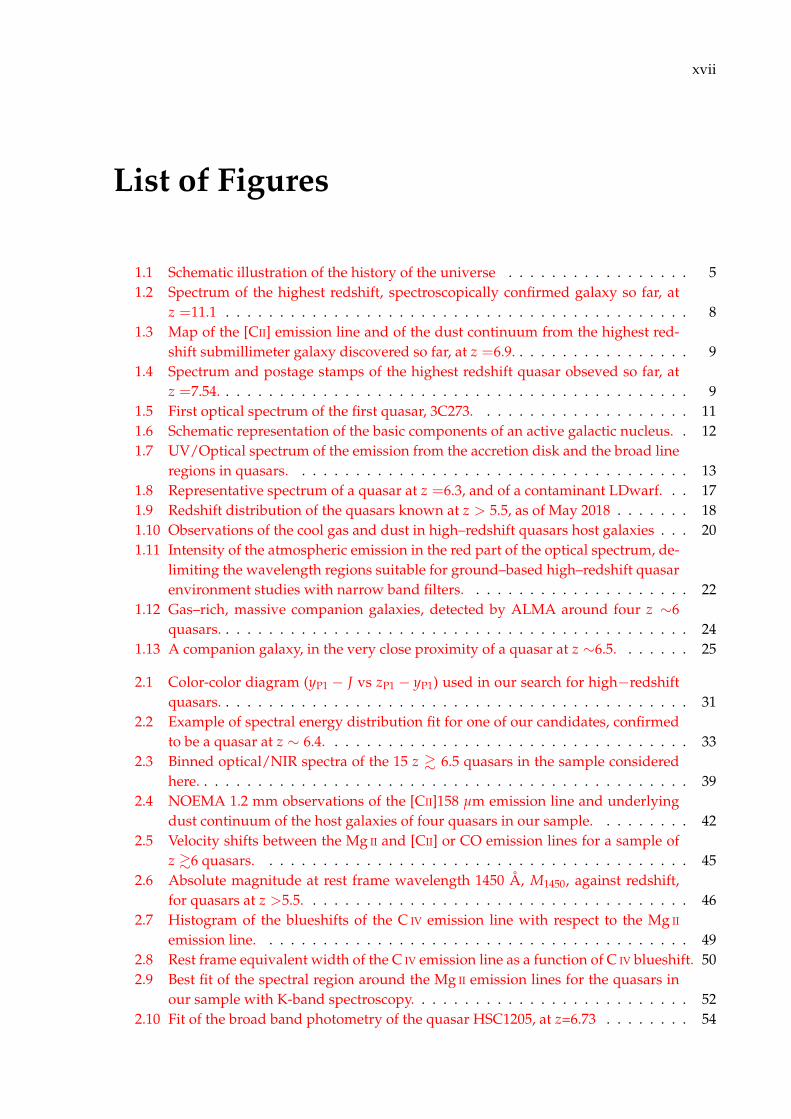
List of Figures
1.1 Schematic illustration of the history of the universe . . . . . . . . . . . . . . . . . 51.2 Spectrum of the highest redshift, spectroscopically confirmed galaxy so far, at
z =11.1 . . . . . . . . . . . . . . . . . . . . . . . . . . . . . . . . . . . . . . . . . . . 81.3 Map of the [CII] emission line and of the dust continuum from the highest red-
shift submillimeter galaxy discovered so far, at z =6.9. . . . . . . . . . . . . . . . . 91.4 Spectrum and postage stamps of the highest redshift quasar obseved so far, at
z =7.54. . . . . . . . . . . . . . . . . . . . . . . . . . . . . . . . . . . . . . . . . . . . 91.5 First optical spectrum of the first quasar, 3C273. . . . . . . . . . . . . . . . . . . . 111.6 Schematic representation of the basic components of an active galactic nucleus. . 121.7 UV/Optical spectrum of the emission from the accretion disk and the broad line
regions in quasars. . . . . . . . . . . . . . . . . . . . . . . . . . . . . . . . . . . . . 131.8 Representative spectrum of a quasar at z =6.3, and of a contaminant LDwarf. . . 171.9 Redshift distribution of the quasars known at z > 5.5, as of May 2018 . . . . . . . 181.10 Observations of the cool gas and dust in high–redshift quasars host galaxies . . . 201.11 Intensity of the atmospheric emission in the red part of the optical spectrum, de-
limiting the wavelength regions suitable for ground–based high–redshift quasarenvironment studies with narrow band filters. . . . . . . . . . . . . . . . . . . . . 22
1.12 Gas–rich, massive companion galaxies, detected by ALMA around four z ∼6quasars. . . . . . . . . . . . . . . . . . . . . . . . . . . . . . . . . . . . . . . . . . . . 24
1.13 A companion galaxy, in the very close proximity of a quasar at z ∼6.5. . . . . . . 25
2.1 Color-color diagram (yP1 − J vs zP1 − yP1) used in our search for high−redshiftquasars. . . . . . . . . . . . . . . . . . . . . . . . . . . . . . . . . . . . . . . . . . . . 31
2.2 Example of spectral energy distribution fit for one of our candidates, confirmedto be a quasar at z ∼ 6.4. . . . . . . . . . . . . . . . . . . . . . . . . . . . . . . . . . 33
2.3 Binned optical/NIR spectra of the 15 z & 6.5 quasars in the sample consideredhere. . . . . . . . . . . . . . . . . . . . . . . . . . . . . . . . . . . . . . . . . . . . . . 39
2.4 NOEMA 1.2 mm observations of the [CII]158 µm emission line and underlyingdust continuum of the host galaxies of four quasars in our sample. . . . . . . . . 42
2.5 Velocity shifts between the Mg II and [CII] or CO emission lines for a sample ofz &6 quasars. . . . . . . . . . . . . . . . . . . . . . . . . . . . . . . . . . . . . . . . 45
2.6 Absolute magnitude at rest frame wavelength 1450 Å, M1450, against redshift,for quasars at z >5.5. . . . . . . . . . . . . . . . . . . . . . . . . . . . . . . . . . . . 46
2.7 Histogram of the blueshifts of the C IV emission line with respect to the Mg II
emission line. . . . . . . . . . . . . . . . . . . . . . . . . . . . . . . . . . . . . . . . 492.8 Rest frame equivalent width of the C IV emission line as a function of C IV blueshift. 502.9 Best fit of the spectral region around the Mg II emission lines for the quasars in
our sample with K-band spectroscopy. . . . . . . . . . . . . . . . . . . . . . . . . . 522.10 Fit of the broad band photometry of the quasar HSC1205, at z=6.73 . . . . . . . . 54

xviii
2.11 Black hole mass as function of bolometric luminosity. . . . . . . . . . . . . . . . . 552.12 Black hole mass, Eddington ratio and bolometric luminosity against redshift. . . 562.13 Distribution of black hole masses, Eddington ratios and bolometric luminosities
for a sample of SDSS z ∼1 quasars matched in bolometric luminosity with oursample. . . . . . . . . . . . . . . . . . . . . . . . . . . . . . . . . . . . . . . . . . . . 57
2.14 Masses of the black hole seeds required to obtain the observed black hole massesin our quasar sample, given different assumptions on black hole accretion. . . . . 60
2.15 Fe II-to-Mg II flux ratio, a first-order proxy for the relative abundance ratio, versusredshift. . . . . . . . . . . . . . . . . . . . . . . . . . . . . . . . . . . . . . . . . . . . 62
2.16 [CII] -to-FIR luminosity ratio, as function of FIR luminosity, in quasars host galax-ies. . . . . . . . . . . . . . . . . . . . . . . . . . . . . . . . . . . . . . . . . . . . . . . 65
2.17 Example of quasar continuum emission fitted with the Principle ComponentAnalysis method. . . . . . . . . . . . . . . . . . . . . . . . . . . . . . . . . . . . . . 67
2.18 Transmission fluxes of the quasars in our sample, as a function of proper distancefrom the source . . . . . . . . . . . . . . . . . . . . . . . . . . . . . . . . . . . . . . 69
2.19 Near zone sizes as a function of redshift. . . . . . . . . . . . . . . . . . . . . . . . . 70
3.1 Set of broad and narrow–band filters used to search for LAEs in the present study. 743.2 RGB composite image of the field around the quasar PSOJ215−16. . . . . . . . . 753.3 Detection completeness function for the sources in our catalog in the narrow
band filter. . . . . . . . . . . . . . . . . . . . . . . . . . . . . . . . . . . . . . . . . . 773.4 Color-Color, (z-NB) vs (R-z), diagram of the sources in our field detected in the
narrow band filter. . . . . . . . . . . . . . . . . . . . . . . . . . . . . . . . . . . . . 783.5 Postage stamps of our LAE candidates. . . . . . . . . . . . . . . . . . . . . . . . . 793.6 Cumulative number counts of LAEs in blank and quasar fields. . . . . . . . . . . 813.7 Equivalent width and Lyα luminosity distribution of the LAEs detected by the
selection criteria in this work, from synthetic templates of LAEs. . . . . . . . . . . 833.8 Velocity distribution of mocked LAEs, that are selected by the criteria in our study. 843.9 Expected number of LAEs, as a function of projected distance from the quasar,
in case of no clustering and from few illustrative clustering scenarios. . . . . . . . 863.10 Color-magnitude diagram (R-z) vs z, for the sources detected in the z band. . . . 883.11 Cumulative Number Counts of LBGs at z∼6, for quasars and blank fields. . . . . 91
4.1 Spectra of the companions of the quasars PJ231 and J0842, acquired with theMagellan/FIRE spectrograph. . . . . . . . . . . . . . . . . . . . . . . . . . . . . . . 96
4.2 Postage stamp of the field around the quasar J2100, imaged with the LUCI1 andLUCI2 cameras at the LBT. . . . . . . . . . . . . . . . . . . . . . . . . . . . . . . . . 100
4.3 HST/WFC3 and Spitzer/IRAC postage stamps of the fields (quasar+companion)considered in this study. . . . . . . . . . . . . . . . . . . . . . . . . . . . . . . . . . 102
4.4 Postage stamps of the archival observations of the field around the quasar J0842. 1034.5 HST/WFC3 native and PSF subtracted images of the quasar PJ167. . . . . . . . . 1034.6 Spectral Energy Distribution of four companion galaxies adjacent to z ∼6 quasars.1074.7 Fraction of obscured star formation as a function of stellar mass. . . . . . . . . . . 1094.8 Star formation rate as a function of stellar mass for a compilation of sources at
z ∼6. . . . . . . . . . . . . . . . . . . . . . . . . . . . . . . . . . . . . . . . . . . . . 1124.9 Postage stamps and spectral energy distribution of a source adjacent to the quasar
J2211, detected solely in the dust–continuum emission. . . . . . . . . . . . . . . . 115

xix
5.1 Regions of quasar parameter space, i.e. black hole masses, redshifts and lumi-nosity, that will be covered with future survey (LSST) and space mission (Euclid). 120
5.2 The quasar PJ323+12 offers an unprecedented opportunity to study the stellarlight and diffuse gas around a quasar at z ∼6.6. . . . . . . . . . . . . . . . . . . . . 123
5.3 Spectral Energy distribution of a quasar and its host galaxy at z =7.54, togetherwith the filter response curves of the NIRCam and MIRI cameras on board JWST. 124
5.4 The JWST/NIRCam instrument offers a unique combination of broad and nar-row band filters for studies of line emitters in the environment of z ∼6.1 quasars. 125


xxi
List of Tables
1.1 Main quasar broad emission lines observed in the rest–frame UV/optical spec-trum. . . . . . . . . . . . . . . . . . . . . . . . . . . . . . . . . . . . . . . . . . . . . 14
2.1 Imaging follow−up observation campaigns for PS1 high−redshift quasar can-didates. . . . . . . . . . . . . . . . . . . . . . . . . . . . . . . . . . . . . . . . . . . . 34
2.2 Spectroscopic observations of the z & 6.5 quasars presented in this study. . . . . . 362.3 PS1 PV3, zdecam, J and WISE photometry and Galactic E(B − V) values of the
quasars analysed here. . . . . . . . . . . . . . . . . . . . . . . . . . . . . . . . . . . 372.4 Photometry from our follow-up campaigns for the newly discovered PS1 quasars. 382.5 Sample of quasars at z & 6.42 considered in this study. . . . . . . . . . . . . . . . 432.6 Parameters from the power law fit of the spectra in our quasar sample; appar-
ent and absolute magnitude at rest frame wavelength 1450; C IV emission lineproperties. . . . . . . . . . . . . . . . . . . . . . . . . . . . . . . . . . . . . . . . . . 47
2.7 Quantities derived from the fit of the spectral region around the Mg II emissionline. . . . . . . . . . . . . . . . . . . . . . . . . . . . . . . . . . . . . . . . . . . . . . 51
2.8 Bolometric luminosities, black hole masses, Eddington ratios, Fe II-to-Mg II fluxratios for the quasars in our sample. . . . . . . . . . . . . . . . . . . . . . . . . . . 59
2.9 Properties of the quasars host galaxies from our observations of the dust andcool gas emission. . . . . . . . . . . . . . . . . . . . . . . . . . . . . . . . . . . . . . 64
2.10 Near zone sizes of 11 quasars in the sample presented here. . . . . . . . . . . . . . 68
3.1 Source names, Coordinates, narrow band magnitudes and projected distances tothe quasar of the Lyman Alpha Emitter candidates in this study. . . . . . . . . . . 78
3.2 Field names, coordinates, effective areas and technical characteristics for the Rand z filters of comparison fields for our LBG search, and the one studied here. . 89
3.3 Characteristics of comparison Fields for our Lyman Break Galaxy selection. . . . 903.4 List of z>5 quasars whose large-scale fields were inspected for the presence of
galaxy overdensities. . . . . . . . . . . . . . . . . . . . . . . . . . . . . . . . . . . . 92
4.1 Characteristics of the quasar+companion systems studied in this work. . . . . . . 974.2 Information on optical/IR spectroscopy and imaging data used in this work. . . 984.3 Photometric measurement of the companion galaxies to z ∼ 6 quasars studied
in this work. . . . . . . . . . . . . . . . . . . . . . . . . . . . . . . . . . . . . . . . . 1044.4 Physical properties of the companion galaxies to z ∼6 quasars studied in this
work. . . . . . . . . . . . . . . . . . . . . . . . . . . . . . . . . . . . . . . . . . . . . 1104.5 Information on a source detected only via its dust continuum emission close to
the quasar VIK J2211−3206. . . . . . . . . . . . . . . . . . . . . . . . . . . . . . . . 114
A.1 List of broad band filters used in this thesis and their characteristics (Telescope/Survey,central wavelength and width). . . . . . . . . . . . . . . . . . . . . . . . . . . . . . 129

xxii
B.1 Objects spectroscopically confirmed to not be high redshift quasars. . . . . . . . . 131

1
Chapter 1
Introduction
In the following chapter, we summarize a few concepts and quantities to provide a usefulbackground for this thesis. We describe the adopted cosmological model (§1.1), and the currentobservational and theoretical view of the Epoch of Reionization (§1.2) and of the first galaxies(§1.3). We then present the history and basic components of quasars (§1.4) and we explorerecent efforts on the discovery and characterization of quasars at high–redshift (§1.5).
1.1 Elements of Cosmology
Here, we briefly set the cosmological framework of the present thesis. The following sectionmakes use of material from Longair, 2008 and Ryden, 2003.
1.1.1 Cosmological Principles and Robertson-Walker Metric
As a first order approximation, we can consider the universe at the present epoch as isotropicand homogeneous. In such a universe, the cosmological principle postulates that any observerdoes not reside in a special location. Additionally, the Weys postulate assumes that no space–time geodesic intersects one another, as they all originated from a single point in the past. Asa consequence, at each point in the universe only one geodesic is found. Considering the twopoints above, it is possible to define a system of fundamental observers, each at a specific cosmictime. In this framework, one can express the metric of the universe as follows.
In general, the distance between two points in a three-space isotropic universe can be for-mulated through the Minkowski metric:
ds2 = dt2 − dl2
c2 (1.1)
with c the speed of light, and dt and dl the time and spatial increment, respectively. The lattercan be expressed in spherical coordinates as:
dl2 = dr2p + R2
c sin2( rp
Rc
)[dθ2 + sin2 θdφ2] (1.2)
where rp is the proper radial distance between two points, and Rc is the space curvature. If weconsider an expanding universe that follows the cosmological principles reported above, thenthe distance between two fundamental observers (j and k) at two different epochs (t1 and t2)follows the relation:
rp,j(t1)
rp,k(t1)=
rp,j(t2)
rp,k(t2)= constant (1.3)

2 Chapter 1. Introduction
We can introduce a universal factor, the scale factor, that summarizes the evolution of this dis-tance between two observers with time, a(t). In this formalism, from eq. 1.3 we derive:
rp,j(t1)
rp,j(t2)=
rp,k(t1)
rp,k(t2)= constant =
a(t1)
a(t2)(1.4)
The proper distance can also be expressed as:
rp(t) = a(t)r (1.5)
with r being the comoving radial distance coordinate. Considering the evolution of the curvatureas Rc(t) = a(t)Rc(t0) = a(t)R, with R the curvature at present epoch, which is necessary topreserve the isotropy and homogeneity of the universe, the metric above becomes:
ds2 = dt2 − a(t)2
c2
[dr2 + R2 sin2
( rR
)[dθ2 + sin2 θdφ2]] (1.6)
This is the so–called Robertson-Walker metric. It is important to notice that this metric is in-dependent of the assumptions on the large scale dynamics of the universe, i.e. the physics ofexpansion, which is contained solely in the factor a(t).
1.1.2 Cosmological Redshift
The cosmological redshift is the shift of emission lines to longer wavelengths associated withthe isotropic expansion of the system of galaxies. Taking into account an emission line withemitted wavelength λe, and observed wavelength λo, the redshift z is calculated as:
z =λo − λe
λe(1.7)
Interpreting the redshift as a galaxy’s recession velocity, we can also write z = v/c (in the ap-proximation of small z). A crucial physical interpretation of the redshift comes directly from theRobertson-Walker metric. If one imposes a radial expansion (dθ=dφ=0) on null cones (ds=0), itis possible to write:
dt =a(t)
cdr (1.8)
Considering a wave packet of frequency ν1, emitted during the time interval [t1,t1 + ∆t1] andobserved at [t0,t0 + ∆t0], and integrating the relation above, one obtains:
∆t0 =∆t1
a(t1)(1.9)
which represents the dilation of time intervals. We can express this relation in terms of observed(ν0 = ∆t−1
0 ) and emitted (ν1 = ∆t−11 ) frequency, and hence:
ν0 = ν1a(t1) (1.10)
All of these considerations lead to the following link between a(t) and redshift:
a(t1) =1
1 + z(1.11)

1.1. Elements of Cosmology 3
The redshift is therefore a measure of the scale factor of the universe at the time of the sourceemission.
In the present thesis, we will focus on cosmic epochs at z >5.5. In the following section, wewill briefly show how the age of the universe and distance measures relate to redshift. First,we will shortly describe the cosmological model and parameters assumed in this thesis.
1.1.3 Hubble Law and Cosmological Parameters
A relation between the distance and recession velocity of nearby galaxies was initially observedby Hubble, 1929. This relation, expressed using the proper distance rp, is:
drp
dt= Hrp (1.12)
where H is the Hubble constant. One can also define the density parameter (Ωx) of the differentcomponents of the universe, i.e. radiation (rad), matter (m) and dark energy (Λ), as:
Ωx =ρx
ρc= ρx
8πG3H0
(1.13)
with ρc the critical density of the universe, and H0 the Hubble constant at present day. Consid-ering the scale factor a(t), the above defined density parameters and a model of the universewith no curvature, one obtains:
H(t) =aa= H0
[Ωma−3 + Ωrada−4 + ΩΛ
]1/2 (1.14)
The radiation density parameter is negligible at the present epoch (Ωrad ∼ 10−4). As for theremaining parameters, in this thesis we consider the matter density parameter (Ωm) equal to0.3, the dark energy density parameter (ΩΛ) equal to 0.7, and H0 =70 km s−1 Mpc−1.
1.1.4 Age of the Universe
It is possible to obtain a measurement of the age of the universe (T) by integrating eq. 1.8:
T =∫
dt =∫ a(t)dr
c(1.15)
The current measurement of the age of the universe at present epoch, considering the cosmo-logical models and parameters reported in eq. 1.1.3, is T0 =13.462 Gyr. As reference for thework in this thesis, the age of the universe at z =5.5,6.0,6.5,7.0,7.5 is T =1.022, 0.914, 0.825,0.748, 0.683 Gyr.
1.1.5 Cosmological Distances
We use several distance measurements in this thesis, that we define below.
Comoving and Proper Distance
The comoving distance (dc) is the distance between two points which takes into account theexpansion of the universe. It does not change with the expansion of the universe, and it is
4 Chapter 1. Introduction
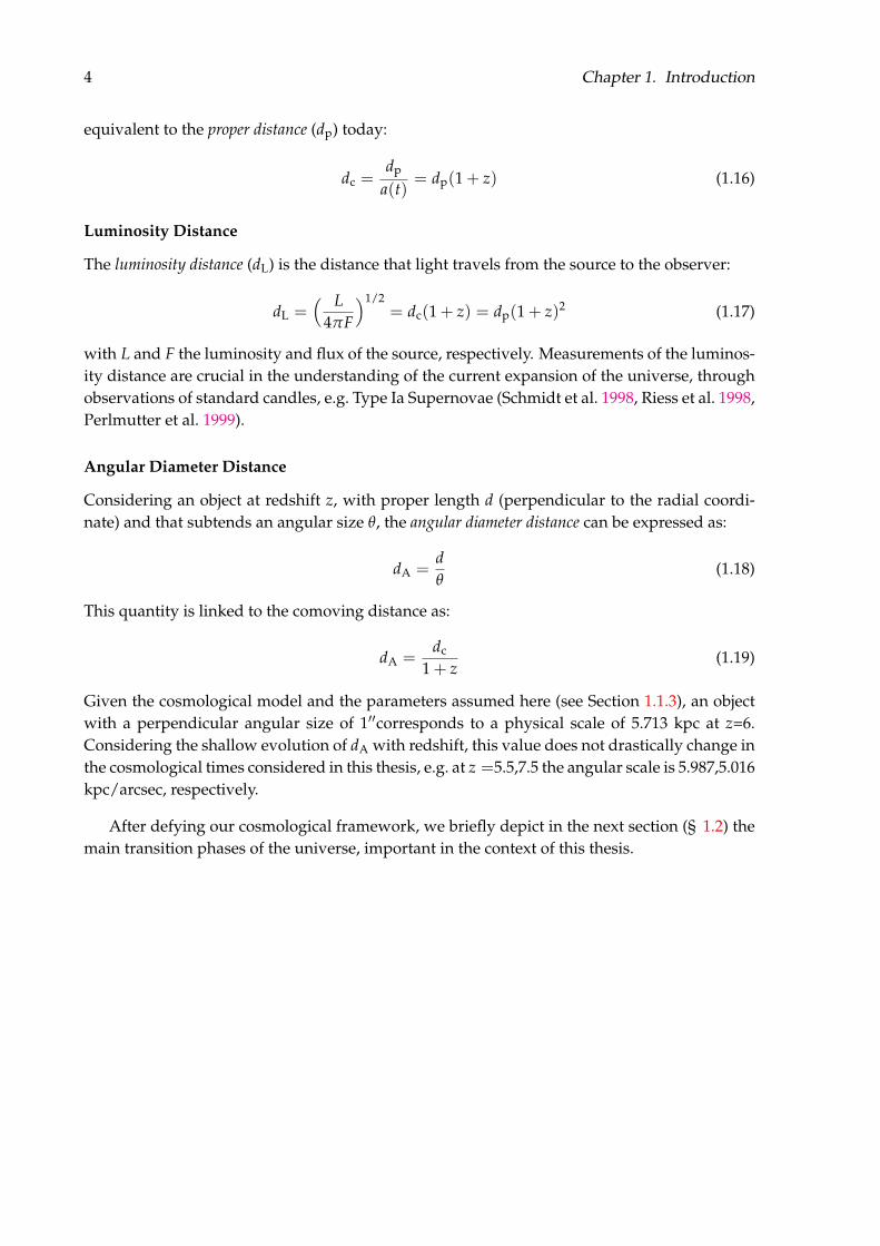
equivalent to the proper distance (dp) today:
dc =dp
a(t)= dp(1 + z) (1.16)
Luminosity Distance
The luminosity distance (dL) is the distance that light travels from the source to the observer:
dL =( L
4πF
)1/2= dc(1 + z) = dp(1 + z)2 (1.17)
with L and F the luminosity and flux of the source, respectively. Measurements of the luminos-ity distance are crucial in the understanding of the current expansion of the universe, throughobservations of standard candles, e.g. Type Ia Supernovae (Schmidt et al. 1998, Riess et al. 1998,Perlmutter et al. 1999).
Angular Diameter Distance
Considering an object at redshift z, with proper length d (perpendicular to the radial coordi-nate) and that subtends an angular size θ, the angular diameter distance can be expressed as:
dA =dθ
(1.18)
This quantity is linked to the comoving distance as:
dA =dc
1 + z(1.19)
Given the cosmological model and the parameters assumed here (see Section 1.1.3), an objectwith a perpendicular angular size of 1′′corresponds to a physical scale of 5.713 kpc at z=6.Considering the shallow evolution of dA with redshift, this value does not drastically change inthe cosmological times considered in this thesis, e.g. at z =5.5,7.5 the angular scale is 5.987,5.016kpc/arcsec, respectively.
After defying our cosmological framework, we briefly depict in the next section (§ 1.2) themain transition phases of the universe, important in the context of this thesis.

1.2. The Epoch of Reionization 5
1.2 The Epoch of Reionization
In Figure 1.1 we show a stylized picture of the history of the universe, from the initial Big Bangto the present day. Approximately ∼400 000 yr after the Big Bang, i.e. at redshift z ∼1100,the temperature of the universe decreased to .3000 K, allowing protons and electrons to re-combine and form neutral hydrogen and helium (Epoch of Recombination). Photons decoupledfrom barions in the primordial plasma, creating the first radiation that nowadays we observeas the Cosmic Microwave Background (CMB). This marked the beginning of the Dark Ages, whenthe diffuse material in the universe was mostly neutral. The gravitational collapse of material,modulated by the primordial density perturbations mapped into the CMB, gave birth to thefirst stars and galaxies. These sources started ionizing the neutral hydrogen in the intergalacticmedium1, firstly in “bubbles” surrounding these sources, and later expanding throughout theuniverse. This is the so–called Epoch of Reionization (EoR), which represents the last major tran-sition phase of the universe (see e.g. Loeb and Barkana 2001, Fan, Carilli, and Keating 2006, Mc-Quinn 2016 and Namikawa 2018 for reviews). At the end of this epoch, the universe emergedas virtually fully ionized, i.e. with a hydrogen neutral fraction of xHI = nHI/nH ∼ 10−5, aswe see it nowadays. Despite the crucial importance of the EoR in the history of the universe,several questions are left unanswered. When did reionization start, and how long did it last? Whatwas its topology? Which were the sources primarily responsible for ionizing the universe? In the lastyears, an extensive effort, both on a theoretical and observational ground, has been undertakenin order to address these issues.
FIGURE 1.1: Simplified illustration of the history of the universe, from the BigBang to the present epoch. The Epoch of Reionization marks the translation froma precedent neutral universe, i.e the Dark Ages, to a mostly ionized one (credits:
NAOJ).
Mapping reionization through a theoretical approach is extremely challenging. Indeed, anysimulation needs to take into account several physical scales. On the one hand, it is necessaryto reproduce the physics of gas accretion and galaxy formation on sub−kpc scales, in orderto characterize the properties (e.g. radiative feedback, metal pollution, star formation) of thefirst sources responsible for producing the initial ionizing radiation. On the other hand, these
1The reionization of helium takes place only afterwards, at z ∼3, and it is believed to be mainly due to the hardradiation emitted by quasars (e.g. Sokasian, Abel, and Hernquist 2002, Furlanetto and Oh 2008; see Ciardi andFerrara 2005 for a review).

6 Chapter 1. Introduction
galaxies need to be located in a cosmological framework, i.e. within the large scale (∼Mpc)dark–matter distribution, where typical inhomogeneities extend up to ∼100 Mpc. In the firstcase, combinations of N-body and hydrodynamical simulations are used, while, in the sec-ond case, radiative transfer techniques are commonly considered (for a recent review on theseapproaches see, e.g., Mesinger 2018).
From an observational perspective, current constraints are obtained from either “integral”probes, e.g. from the CMB or galaxies number counts, or individual sources that act as ”light-houses”, that provide us information on specific lines of sight. As for the first case, recently,the Planck Collaboration et al., 2016 measured the Thomson scattering optical depth from theCMB, and set a redshift of z=8.8+1.3
−1.2 for the EoR, under the assumption that reionization wasinstantaneous. Regarding the sources responsible for the initial re-ionization, a number of con-straints from observations of large samples of UV–bright galaxies at z >6 (see also Section 1.3)suggest that the main drivers for the EoR were faint star forming galaxies (e.g. Bouwens et al.2015a and references therein; but see also, e.g. Giallongo et al. 2015, for an alternative view).
Luminous high–redshift quasars, i.e. the aforementioned “lighthouses”, are key probes ofthe EoR. Indeed, observations of z >5.5 quasars firstly set the end of reionization at z ∼6(e.g. Fan et al. 2006, McGreer, Mesinger, and D’Odorico 2015). Moreover, even one quasarfound at z >7 can provide stronger constraints on the hydrogen neutral fraction value, at oneredshift and on one line-of-sight, than what obtained from CMB measurements (e.g. Bañadoset al. 2018). In Section §1.5, we report in greater details the methods through which high–zquasars can constrain the onset, duration and morphology of reionization.We start by summarizing the current census of the sources observed at the edge of the EoR(z &6) in the next Section (§ 1.3).
1.3 The First Galaxies
In the last years, several studies have been undertaken that search for the first galaxies.
One way of identifying such galaxies is through deep, extragalactic photometric surveys,which observe the rest–frame ultraviolet (UV) and/or optical emission from young stars andionized nebular gas. Such searches can be performed via, e.g., the Lyman Break technique(identifying drop-outs or Lyman Break Galaxies, LBGs): absorption by intergalactic neutral hy-drogen causes a break in the observed galactic spectrum, apparent from abrupt change inbroad–band colors (e.g. Steidel et al. 1996). LBGs, selected with this method from ground–based facilities, are massive sources, characterized by strong UV stellar emission, and whosemass strongly correlates with the UV luminosity (e.g. González et al. 2011). On the other hand,suites of narrow and broad band filters efficiently identify Lyα Emitters (LAE), via the observa-tions of the Lyα emission line. LAEs are believed to be mostly low-mass galaxies, spanning arange of stellar masses of ∼ 106−108 M and ages of ∼1−3 Myr (e.g. Pirzkal et al. 2007, Onoet al. 2010). However, a non negligible fraction of massive galaxies (with masses up to ∼1011
M), and galaxies hosting an older stellar population (∼ 1 Gyr) has been also found amongLAEs (e.g. Pentericci et al. 2009, Finkelstein et al. 2009, Finkelstein et al. 2015a). Recent theoret-ical and observational studies suggest that LBGs and LAEs trace a similar underlying galaxy

1.3. The First Galaxies 7
population, with the main difference between the two arising from the diverse selection meth-ods (e.g. limits on the UV luminosity and equivalent width of the line; e.g. Garel et al. 2015).
Deep observations with the Hubble Space Telescope (HST) and the Spitzer Space Telescope wereinstrumental in shaping our knowledge of such galaxy population. More than 800 galaxy can-didates have been identified with photometric redshifts at z ∼7–8 (e.g. Schmidt et al. 2014,Finkelstein et al. 2015b, Bouwens et al. 2015b), and even at z ∼9–10 (e.g. McLeod et al. 2015,Kawamata et al. 2016). Conversely, several ground–based surveys with narrow band filters at,e.g. the Subaru Telescope or the Very Large Telescope (VLT), detected a large number of LAEs atz ∼ 6− 7 (e.g. Ouchi et al. 2018, 2008, Ono et al. 2010, Hu et al. 2010). Nevertheless, only a smallfraction of all these galaxies were spectroscopically confirmed at z >7 (e.g. Vanzella et al. 2011,Ono et al. 2012, Shibuya et al. 2012, Finkelstein et al. 2013, Zitrin et al. 2015, Roberts-Borsaniet al. 2016).
The most distant galaxy was observed so far at z =11.09 (Oesch et al. 2016; see Figure 1.2).Even if this galaxy is extremely bright (i.e. its UV luminosity is 3×L* of z ∼7-8 dropouts2), itsspectroscopic detection is still tentative, and little information on its physical properties can bederived from its observations. In general, the Lyα emission line is difficult to detect. It is highlyaffected by absorption and scattering (both in spatial and velocity space) by the intervening in-tergalactic medium (IGM), and the galactic interstellar medium (ISM). Its escape fraction fromgalaxies, and therefore our ability to detect it, is strongly dependent on the geometry, ioniza-tion state and composition of the ISM. The Lyα line is also rapidly absorbed by the IGM, evenin case of low hydrogen neutral fraction (i.e. xHI &10−4). Moreover, spectroscopic confirmationand study of other emission lines from the ISM of these very distant UV–selected galaxies isextremely challenging.
An alternative approach to uncover the first galaxies is through the emission of their coolgas and dust in the rest–frame far-infrared (FIR). Several blind surveys scanned the sky withe.g. the SCUBA camera at the James Clerk Maxwell Telescope (JCMT), and with MAMBO at theIRAM 30m telescope (e.g. Hughes et al. 1998,Ivison et al. 2000). These surveys detected mul-tiple submillimeter galaxies (SMGs; e.g. Blain et al. 2002), characterized by large infrared (IR)luminosities (LIR > 1012 L) from the dust emission, and large star formation rates (SFR ∼1000M yr−1). The singly ionized [CII]158 µm emission line is an extensively used key diagnosticsof galactic physics in these sources (see Carilli and Walter 2013 and Díaz-Santos et al. 2017for reviews). The [CII] line is indeed one of the main coolant of the ISM, and it can be ex-tremely bright, i.e. it can emit up to 1% of the total galactic infrared emission (e.g. see Herrera-Camus et al. 2018a,b). Further observations of this line and of the dust continuum with the At-acama Large Millimeter Array (ALMA), revealed that SMGs are extended (∼few kpc), heavilydust obscured and typically surrounded by companions/overdensities (e.g. Hodge et al. 2013,Zavala et al. 2017). These galaxies are fundamental in shaping our understanding of galaxyformation and in sampling the gas content and star formation activity in the early universe(e.g. Chapman et al. 2005). Indeed, they have been invoked as possible progenitors of massive,compact, “red and dead” galaxies, already observed at z >2 (e.g. van Dokkum et al. 2008) upto z ∼4 (e.g. Straatman et al. 2014). Indeed, these progenitor galaxies would undergo gas–rich,
2where L* is the characteristic luminosity, defined from the luminosity function (LF): φ(L) =(φ∗/L∗)(L/L∗)α exp−(L/L∗); see Bouwens et al. 2015b and Finkelstein et al. 2015b for LFs of z ∼7-8 galaxies.

8 Chapter 1. Introduction
FIGURE 1.2: The 2D (top) and 1D (bottom panel) spectrum of GN-z11, the mostdistant galaxy with confirmed spectroscopic redshift so far, at z =11.09. The
figure is taken from Oesch et al., 2016
massive mergers, that are expected to ignite powerful, heavily dust-enshrouded starbursts,with the possible formation of a central quasar. In later stages, the formation of new stars isprevented by the feedback from the quasar and/or by gas exhaustion; after the dissipation ofthe dust, and the dimming of the quasar, the central compact remnant can further redden andgrow through dry mergers, building the observed “red and dead” galaxies (e.g. Hopkins et al.2008, Wuyts et al. 2010, Toft et al. 2014).However, up to now, only few SMGs, without a central active black hole, have been found atz >6. Riechers et al., 2013 found a dust-obscured, extremely star forming (SFR ∼3000 Myr−1) SMG at z=6.3; Fudamoto et al., 2017 recovered another SMG at z=6.03, slightly less star-forming (SFR ∼950 M yr−1). The highest redshift pair of massive SMGs has been observedby Marrone et al., 2018 at z ∼6.9 (see Figure 1.3). This very small sample is still too limited tostudy galaxy formation at early cosmic times.
Finally, quasars, due to their extreme brightness, have been observed up to z =7.5413 (Baña-dos et al. 2018, Venemans et al. 2017; see Figure 1.4). Their rest–frame UV spectra harbor awealth of information regarding, e.g. the central black hole, their chemical abundance, andaccretion mode. Moreover, their hosts galaxies are among the most massive, gas rich and star-forming sources in the early universe. Quasars are therefore not only unique probes of the stateof the IGM in the EoR, but they can also shed light on the (co-)evolution of the first galaxiesand black holes.
In the following section (§1.4), we summarize the discovery and basic physical componentsof quasars. In section §1.5, we report the main characteristics of z >5.5 quasars, and of theirhost galaxies and environments, prior to this work.

1.3. The First Galaxies 9
FIGURE 1.3: Map of the [CII] emission line (color map) and dust continuum (con-tours) in the highest redshift submillimeter galaxy, observed at z ∼6.9 (figure
adapted from Marrone et al. 2018).
FIGURE 1.4: Rest–frame UV spectrum, and postage stamps, of the highest red-shift quasar obseved so far, at z =7.5413. Figure adapted from Bañados et al.,
2018.

10 Chapter 1. Introduction
1.4 Quasars: Discovery and Basic Elements
Quasars are among the most luminous, non-transient sources in the sky. The term “quasar”was first created as the acronym of “quasi–stellar radio source”, due to the original, radio-based discoveries. When, in the following years, an increasing number of quasars with noradio emission was found (Sandage, 1965), the word “QSO”, e.g. “quasi–stellar object”, wasintroduced instead. Nowadays, the two terms are used as synonyms.
1.4.1 The Discovery of the First Quasars
The development of the first radio techniques for astronomy, during the fifties and sixties,opened a new window on the observable universe. The first radio surveys, such as the thirdCambridge catalog of radio sources (3C; Edge et al. 1959), identified several radio sourcesdistributed homogeneously over the sky, which were assumed to be of extragalactic origin(e.g. Baade and Minkowski 1954). Thanks to the technique of lunar occultations, Hazard,Mackey, and Shimmins, 1963 measured the location of the radio source 3C 273, with a, at thattime unprecedented, uncertainty of 2′′. Schmidt, 1963 identified a 13th magnitude “stellar–like”object as its optical counterpart. In the optical spectrum obtained at the Palomar 5m Telescope,he was able to reconstruct the Balmer emission line series redshifted at z =0.16 (see Figure 1.5).This result suggested that the source was located at large, cosmological distances, and it wascharacterized by extreme luminosities. 3C273 was the first discovered quasar (for a completereconstruction of the events leading to this discovery, we refer to Hazard et al., 2018). Shortlyafterwards, the object 3C48 was also identified as a similar point–like source at z =0.37 (Green-stein, 1963). In the same fashion, many more quasars were discovered from radio catalogs inthe following years, followed by sources which were not characterized by any radio emission(e.g. Sandage 1965, Schmidt 1966). Quasars quickly revolutionized the understanding/view ofthe universe at that time, both greatly expanding the horizon of the observable universe (i.e. thefirst quasar at z ∼2 was discovered only 2 years after 3C273; Sandage 1965), and challengingthe known physics, with compact sizes and significant luminosity variabilities that could not beexplained by the sole stellar radiation (e.g. Smith and Hoffleit 1963). After significant observa-tional and theoretical efforts, a good understanding of the structure and emission mechanismof quasars has been achieved.
1.4.2 Quasars Basic Components
Quasars are thought to be mainly composed by:
• A central, supermassive black hole (SMBHs; 107 . MBH/M . 1010)
• A surrounding accretion disk, i.e. material with non-null angular momentum, being ac-creted by the black hole and emitting a large amount of energy in the rest–frame UV/opticalrange.
• A broad line region, BLR, composed by high-velocity gas “clouds” in the proximities ofthe black hole.
• A X-ray corona, a hot (T& 107 K) region above and below the accretion disk, stronglyemitting in the X–ray regime.

1.4. Quasars: Discovery and Basic Elements 11
FIGURE 1.5: Discovery spectrum, acquired with the Palomar 5m Telescope, of thefirst quasar 3C273, at z =0.16. The figure is adapted from Hazard et al., 2018.
• An obscuring, dusty torus, found at several pc from the black hole, absorbing part of theenergy from the accretion disk, and re-emitting it in the infrared (λ ∼3 µm) range.
• A narrow line region, NLR, gas regions observed at larger distances (∼0.1 kpc), movingat velocities of∼300–500 km s−1, and producing narrow emission lines in the UV/opticalspectrum.
• Two powerful jets, which convey materials moving at relativistic speed; they are thoughtto be present in the 10%–20% of the objects.
All these elements are visually summarized in Figure 1.6.
In this thesis, we will mainly focus on the characterization of the central black holes and ofthe emission from the accretion disk and the BLR in high–redshift quasars, via observations oftheir rest–frame UV spectra. We provide here few additional details on the latter two compo-nents. This discussion is mainly adapted from Ghisellini, 2013 and Vanden Berk et al., 2001.We also list current methods of measuring MBH in the next section (§ 1.4.3).
The accretion disk is composed of matter infalling into the central black hole, which, whileloosing angular momentum, is emitting radiation as:
Ldisk = εMBHc2 (1.20)
where ε is the radiative efficiency, usually around 10%, and MBH is the mass accretion rate. As-suming that this structure can be divided in annuli emitting black body radiation, than the totalaccretion disk emission can be modeled as a sum of black bodies with different temperatures,with higher temperatures closer to the black hole:
T(R) =[
3RSLdisk
16πσMBR3
]1/4[1−
(3RS
R
)1/2]1/4
∝ R−3/4 if R >> RS
(1.21)

12 Chapter 1. Introduction
FIGURE 1.6: Schematic representation of an active galactic nucleus (AGN) basiccomponents, which are listed in Section 1.4.2 (adapted from Urry and Padovani
1995).
where σMB is the Maxwell–Boltzmann constant, and RS = 2MBHG/c2 is the Schwarzchild ra-dius. No radiation is emitted from orbits with R ≤ 3RS. Assuming that each annuli emitsluminosity as:
dL = 4πRdRσMBT4 (1.22)
and considering only the peak frequency corresponding to the black body temperature (hν ∝kT), one can derive:
Ldisk ∝ ν1/3 (1.23)
This is valid up to the limit set by the maximum temperature, close to the internal radius (Rin)of the accretion disk. In this case, we will observe only an exponential drop (Ldisk ∝ exphν/kT).On the other hand, only the Rayleigh-Jeans contribution will be observed at the outer radius(Rout; Ldisk ∝ ν2). We show all this components in Figure 1.7, right.In the present work, we will model the emission from the quasars accretion disks with a powerlaw relation (see Section 2.5.3).
Another important quantity is the Eddington luminosity, i.e. the theoretically maximum lu-minosity permitted for the quasar. This quantity is derived assuming that: 1) the radiationpressure and the gravitational attraction are in equilibrium (Frad = Fg); 2) the radiation pres-sure acts on electrons through the Thomson scattering, while the gravitational force acts on theprotons; 3) the black hole accretion is spherically symmetric (i.e. Bondi accretion; Bondi 1952).

1.4. Quasars: Discovery and Basic Elements 13
FIGURE 1.7: Left: Theoretical models of the spectrum of a quasar accretion disk,following a power law form, in case of different values of maximum radii. Right:Main broad (an narrow) emission lines in the UV/optical wavelength window,observed in the composite spectrum obtained using a sample of SDSS quasars.
The figures are adapted from Ghisellini, 2013 and Vanden Berk et al., 2001.
From these assumptions, we can write:
LEddσT
4πR2c=
GMBHmp
R2 (1.24)
from which we derive
LEdd =4πGmp
σT·MBH = 1.3× 1038 MBH
M(1.25)
with σT the Thomson scattering section and mp the proton mass. Even considering the strictaforementioned assumptions, the Eddington limit seems to be generally respected among theobserved AGNs, i.e. no black hole has been observed so far whose luminosity largely andsecurely surpasses the Eddington one (e.g. Trakhtenbrot, Volonteri, and Natarajan 2017; Bianand Zhao 2003). Also, one can define the Eddington ratio, i.e. the ratio between the bolometric(Lbol) and the Eddington luminosity (Lbol/LEdd). The Eddington ratio is commonly considereda proxy of the efficiency of matter accretion onto the central SMBH.We will largely make use of LEdd and its relation with the quasar bolometric luminosity in thepresent thesis.
In Figure 1.7, left, we show an example of emission from broad lines, overimposed to thecontinuous radiation from the accretion disk. In Table 1.1, we report the rest–frame wave-lengths of the main emission lines, that we will utilize in the present work. The BLRs arecomposed by gaseous regions with a temperature of ∼ 104 K, a density of ∼ 109 − 1011 cm−3,and a covering factor of ∼0.1 (e.g. Ghisellini 2013). The full widths at half maximum (FWHM)of the lines are typically 1000–10,000 km s−1, while the sizes of the BLRs are RBLR ∼ 0.1pc(e.g. Peterson et al. 2004; see also Section 1.4.3)

14 Chapter 1. Introduction
TABLE 1.1: Main quasar broad emission lines observed in the rest–frameUV/optical spectrum. The laboratory wavelength of the rest frame emission andthe relative strenght of the line with respect to that of Lyα are taken from Vanden
Berk et al., 2001.
ID λrest Relat. Flux[Å] [100×F/F(Lyα)]
Lyβ 1025.72 9.615 ± 0.484Lyα 1215.67 100.000 ± 0.753NV 1240.14 2.461 ± 0.189SiV 1396.76 8.916 ± 0.097CIV 1549.06 25.291 ± 0.106MgII 2798.75 14.725 ± 0.030Hβ 4862.68 8.649 ± 0.030Hα 6564.61 30.832 ± 0.098
1.4.3 Black Hole Masses Estimates
The mass of the central black hole can be estimated through direct (i.e. primary) or indirect(i.e. secondary) approaches. The black hole in our Galactic center is the closest and best studiedone, and orbits of individual stars have been extensively used to measure its mass (e.g. Genzel,Eisenhauer, and Gillessen 2010). Among the primary methods, one can find high-resolutionspectroscopic observations of gas and stars in the SMBH sphere of influence (e.g. Tremaine etal. 2002), or, alternatively, accurate water megamasers measurements (e.g. Miyoshi et al. 1995).However, these techniques can be applied only to very nearby and relatively low luminositysources, for which the stellar emission from the host galaxy is not outshone by the central AGN(e.g. Vestergaard 2004). They are therefore unsuitable for surveys of luminous quasars at largecosmological distances.
Alternatively, one can rely on reverberation mapping (RM) techniques (e.g. Peterson et al.2004, Peterson and Horne 2004). RM exploits the time delay (lag) between the flux variationobserved in the emission from the continuum and that from the broad emission lines, in orderto place constraints on the geometry and size of the BLR. RM campaigns in the local universe(e.g. Kaspi et al. 2005, Bentz et al. 2013) found that RBLR strongly correlates with the sourceluminosity:
Log(
RBLR
ltday
)= K + αLog
(λLλ
1044 erg s−1
)(1.26)
This method, together with the assumption that the BLR clouds are in virial equilibrium, al-lowed for the measurements of a large sample of black hole masses (e.g. Shen et al. 2016, Grieret al. 2017), up to redshift z ∼1 (e.g. Shen et al. 2015). Nevertheless, its application at even largercosmological distances is challenging. Indeed, on one hand, the time dilation renders the neces-sary observations much longer (i.e. years), and, on the other, the larger masses sampled at highredshifts are characterized by smaller, and therefore harder to detect, flux variations (e.g. Liraet al. 2018).
It is possible to measure MBH in z >1 quasars via observations of their single–epoch, rest–frame UV/optical spectra, and by adopting again the virial argument and the scaling relations
1.4. Quasars: Discovery and Basic Elements 15
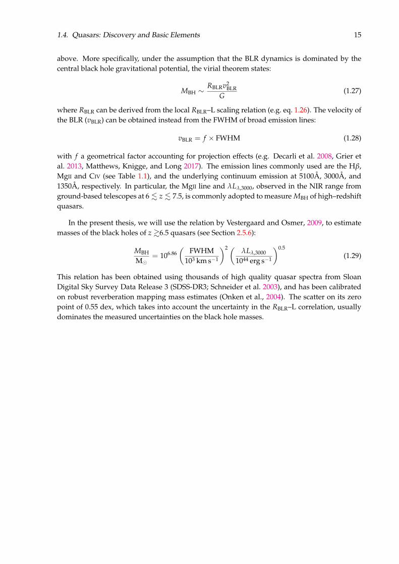
above. More specifically, under the assumption that the BLR dynamics is dominated by thecentral black hole gravitational potential, the virial theorem states:
MBH ∼RBLRv2
BLRG
(1.27)
where RBLR can be derived from the local RBLR–L scaling relation (e.g. eq. 1.26). The velocity ofthe BLR (vBLR) can be obtained instead from the FWHM of broad emission lines:
vBLR = f × FWHM (1.28)
with f a geometrical factor accounting for projection effects (e.g. Decarli et al. 2008, Grier etal. 2013, Matthews, Knigge, and Long 2017). The emission lines commonly used are the Hβ,MgII and CIV (see Table 1.1), and the underlying continuum emission at 5100Å, 3000Å, and1350Å, respectively. In particular, the MgII line and λLλ,3000, observed in the NIR range fromground-based telescopes at 6 . z . 7.5, is commonly adopted to measure MBH of high–redshiftquasars.
In the present thesis, we will use the relation by Vestergaard and Osmer, 2009, to estimatemasses of the black holes of z &6.5 quasars (see Section 2.5.6):
MBH
M= 106.86
(FWHM
103 km s−1
)2 ( λLλ,3000
1044 erg s−1
)0.5
(1.29)
This relation has been obtained using thousands of high quality quasar spectra from SloanDigital Sky Survey Data Release 3 (SDSS-DR3; Schneider et al. 2003), and has been calibratedon robust reverberation mapping mass estimates (Onken et al., 2004). The scatter on its zeropoint of 0.55 dex, which takes into account the uncertainty in the RBLR–L correlation, usuallydominates the measured uncertainties on the black hole masses.

16 Chapter 1. Introduction
1.5 High–Redshift Quasars
In the present thesis, we refer to “high–redshift quasars” for the quasars at z > 5.5. Colorselection techniques, which rely on multi-wavelength broad band observations, are among themost commonly used methods to find high–redshift quasars. The quasar flux at wavelengthsshorter than the Lyα emission line is absorbed by the intervening neutral medium, causingan extremely red (i − z) or (z − y) color if the source is at z & 6 (i−dropouts) or z & 6.4(z−dropouts), respectively. The main contaminants in such selection are cool stars in our ownGalaxy, i.e. M/L/T Dwarf, which present similar red colors at shorter wavelength. In Figure 1.8we show a representative spectrum of a quasar at z =6.3, together with an illustrative spectrumof a stellar contaminant. Information at longer wavelength, i.e. in the near-infrared (NIR) range,where the spectral signatures differ, are needed to reject any foreground Galactic contaminant.Moreover, high–redshift quasars are extremely rare. If one integrates the luminosity functionprovided by Willott et al. 2010b, at z =6, and down to an absolute UV magnitude at rest frame1450 Å of M1450 = −25, one obtains a quasar number count of only ∼0.7 Gpc−3. Therefore, inorder to find high–redshift quasars, observations in the optical/NIR regime on a wide sky areaare necessary.
The first quasar at z=5.5 was discovered ∼20 years ago by Stern et al., 2000. Since then, inthe last two decades, 254 quasars have been discovered at z > 5.5. This was made possible bythe advent of several large-area surveys:
• the Dark Energy Camera Legacy Survey (DECaLS, 1 quasar; Wang et al. 2017)
• the Infrared Medium Deep Survey (IMS, 1 quasar; Kim et al. 2015)
• the Very Large Telescope Survey Telescope (VST) ATLAS Survey (2 quasars; Carnall et al.2015);
• the NOAO Deep Wide-Field Survey (NDWFS, 3 quasars; Cool et al. 2006, McGreer et al.2006)
• the UK Infrared Deep Sky Server (UKIDSS, 9 quasars;Venemans et al. 2007, Mortlock et al.2009, 2011, Bañados et al. 2018);
• the Dark Energy Survey (DES, 10 quasars; Reed et al. 2015, 2017);
• the VISTA Kilo-Degree Infrared Galaxy Survey (VIKING) and the ESO public Kilo DegreeSurvey (KiDS, 13 quasars in total; Venemans et al. 2013, 2015);
• the Canada-France High-redshift Quasar Survey (CFHQS, 20 quasars; Willott et al. 2007,2009, 2010,b);
• the Sloan Digital Sky Survey (SDSS, 52 quasars; Fan et al. 2000, 2003, 2006, Zeimann et al.2011, Jiang et al. 2016, Wang et al. 2016, 2017);
• the Subaru Hyper Suprime-Cam-SPP Survey (HSC-SPP, 64 quasars; Kashikawa et al. 20153,Matsuoka et al. 2016, 2018, 2018)
3This study used the Suprime-Cam.

1.5. High–Redshift Quasars 17
• the Panoramic Survey Telescope and Rapid Response System (Pan-STARRS1 or PS1, 78 quasars;Morganson et al. 2012, Bañados et al. 2014, 2015, 2016, Venemans et al. 2015b, Tang et al.2017).
The current redshift record–holder, J1342+0928 at z = 7.5, was recently discovered by Bañadoset al. (2018; see Figure 1.4). We refer to Section 2.2.1 for an further description of some of thesesurveys. The redshift distribution of all the z >5.5 quasars known at the time of this work isshown in Fig. 1.9.
0.7 0.8 0.9 1.0 1.1 1.2 1.3 1.4 1.50.0
0.2
0.4
0.6
0.8
1.0
1.2
1.4
1.6
1.8
1.4 1.6 1.8 2.0 2.2 2.4 2.60.0
0.5
1.0
1.5
3.0 3.5 4.0 4.5 5.0 5.5 6.0
Observed Wavelength [µm]
0.0
0.5
1.0
QSO@z = 6.3LDwarf
Lyα
SiV
CIV
iP1 zP1 yP1 J
MgIIH K
Hβ HαW1 W2
Flu
x[a
rbit
rary
un
its]
FIGURE 1.8: Representative spectrum of a quasar at z =6.3, obtained by shiftingthe lower−z template from Selsing et al., 2016. Overplotted, we show the spec-trum of a cool dwarf star, one of the main contaminants in high–redshift quasarsearches, and the response curves of the broad band filters primarily used in this
work. The main broad emission lines (see Table 1.1) are also highlighted.
1.5.1 The First Supermassive Black Holes
High–z quasars already host SMBHs with MBH & 109M in their centers. These observa-tions challenge current models of formation and evolution of early supermassive black holes

18 Chapter 1. Introduction
5.5 6.0 6.5 7.0 7.5Redshift
0
5
10
15
20
25
30
35N
um
ber
ofQ
uas
ars
OTHER
SDSS
CFHQS
HSC
VIKING
UKIDSS
PS1
FIGURE 1.9: Redshift distribution of the quasars known at z > 5.5, as of May2018. With “OTHER”, we indicate the objects discovered by the remaining sur-
veys listed in Section 1.5.
(e.g. Volonteri 2010, Latif and Ferrara 2016 for reviews). The current preferred models includethe formation of black hole seeds from the direct collapse of massive gaseous reservoirs (e.g.,Haehnelt and Rees 1993, Latif and Schleicher 2015), the collapse of Population III stars (e.g.,Bond, Arnett, and Carr 1984, Alvarez, Wise, and Abel 2009, Valiante et al. 2016), the co-actionof dynamical processes, gas collapse and star formation (e.g., Devecchi and Volonteri 2009), orthe rapid growth of stellar-mass seeds via episodes of super-Eddington, radiatively inefficientaccretion (e.g., Madau, Haardt, and Dotti 2014, Alexander and Natarajan 2014, Pacucci, Volon-teri, and Ferrara 2015, Volonteri et al. 2016, Lupi et al. 2016, Pezzulli, Valiante, and Schneider2016, Begelman and Volonteri 2017). While the black hole seeds from Pop III stars are expectedto be relatively small (∼ 100 M; e.g. Valiante et al. 2016), and to be formed at earlier times(20 < z < 50), direct collapse of massive clouds can lead to the formation of more massiveseeds (∼ 104 − 106 M) at lower redshifts (8 < z < 10; e.g. Volonteri 2010). On the otherhand, dynamical processes between stars and gas are expected to form ‘intermediate seeds’(∼ 103M) at intermediate times (10 < z < 15). From black hole growth theory, we know thatblack holes can evolve very rapidly from their initial seed masses, MBH,seed, to the final massMBH,f. Indeed, we can express the black hole growth as:
MBH,f = MBH,seed exp(
tts× 1− ε
ε× Lbol
LEdd
)(1.30)

1.5. High–Redshift Quasars 19
with ts =0.45 Gyr is the Salpeter time. Assuming accretion at the Eddington limit, i.e. Lbol =
LEdd, and a radiative efficiency of 10% (Volonteri and Rees, 2005), we obtain:
MBH,f ∼ MBH,seed e9× t [Gyr]0.45 (1.31)
For instance, in the seemingly short redshift range z ∼ 6.0− 6.5, corresponding to ∼ 90 Myr,a black hole can grow by a factor of six. From an observational perspective, the discoveryof quasars at z &6.5 can give stronger constraints on the nature of black hole seeds than thequasar population at z ∼ 6. In this thesis, we will derive MBH estimates for a sample of z >6.5quasars, and place constraints on the respective seed formation. Moreover, observations of theinnermost regions of z > 6 quasars (i.e. the BLR) highlight how these objects have alreadymetallicities close to solar (e.g., Barth et al. 2003, Stern et al. 2003, Walter et al. 2003, De Rosaet al. 2011, De Rosa et al. 2014). Here, we will derive an estimate of the BLR [metal/α elements]abundances from rest–frame UV spectra of z &6.5 quasars.
1.5.2 The Host Galaxies of Distant Quasars
Most quasars at z ∼6 are already hosted in massive gas–rich galaxies. The bright, non thermalemission from the central engine outshines the stellar radiation from the host galaxy, ham-pering so far any attempt to recover the rest–frame UV/optical emission from such galaxies(e.g. Mechtley et al. 2012, Decarli et al. 2012). On the other hand, a large number of studiesobserved conspicuous amounts of cool gas and dust in quasars’ hosts, thanks to the detec-tion of the bright [CII]158 µm emission line and the underlying dust continuum, falling in themillimeter regime at z & 5.5 (see Figure 1.10; e.g., Maiolino et al. 2009, Walter et al. 2009,Willott, Bergeron, and Omont 2015, Venemans et al. 2016, Venemans et al. 2017; for a reviewsee Carilli and Walter 2013). These IR–luminous galaxies (LIR ∼ 1011 − 1012 L) show typicaldust masses of ∼ 108 − 109M, dynamical masses of ∼ 1010 − 1011M, and star formationrates of few 100s M yr−1 (e.g. Decarli et al. 2018). They are characterized by a variety ofmorphologies/kinematics, from rotation disks (e.g. Wang et al. 2013, Venemans et al. 2016), todisturbed/merger-like structures (e.g. Willott, Bergeron, and Omont 2017, Decarli et al. 2017),or compact, unresolved emissions (e.g. Venemans et al. 2017). In this thesis, we will presentnew mm–observations of four quasar host galaxies at z & 6.5, and place their properties in thecontext of quasars and galaxies at low and high–redshifts.
1.5.3 Quasars as probes of the IGM in the EoR
Studies of z ∼5.7 quasars show that they live in a mostly ionized universe: Fan et al., 2006pioneered the use of high–z quasars spectra as probes of the state of the early universe.The most commonly used methods nowadays are:
• the measure of the transmission spikes in the Lyα forest, i.e. the absorption pattern in high–zquasars spectra bluewards of Lyα due to the intervening IGM. This technique permits toestimate the evolution of the Gunn-Peterson optical depth with redshift (e.g. Fan et al.2006, Becker et al. 2015, Barnett et al. 2017), but it is hampered by the fast saturation ofthe Lyα emission line, which is already completely absorbed in case of a hydrogen neutralfraction of xHI ∼ 10−4. Analysis of the Lyβ and Lyγ forests are therefore necessary inorder to probe environments with higher gas neutral fractions, i.e. well into the EoR.

20 Chapter 1. Introduction
FIGURE 1.10: Examples of quasars host galaxies observed in the mm regime.Left: ALMA observations of the [CII] emission line total intensity map, and gasvelocity map, of two z ∼6 quasars (Wang et al., 2013). Right: Spectrum of the[CII] emission line of J0305 at z = 6.6 (top), and its [CII] and underlying contin-
uum intensity map (bottom; Venemans et al. 2016).
• the study of the Lyα power spectrum, using a statistically significant sample of quasars(e.g., Palanque-Delabrouille et al. 2013).
• the analysis of the damping wing in quasars spectra. If the source is surrounded by mostlyneutral gas, the ‘Gunn-Peterson’ absorption is detected, which is extended on the redside of the Lyα line mainly due to the intrinsic width of the line (e.g. Miralda-Escudé1998). This signature has been observed in the spectra of the two highest redshift quasarsknown so far, J1120 and J1342, and, recently, it has been modeled in order to characterizethe state of the surrounding IGM (e.g. Greig et al. 2017, Bañados et al. 2018, Davies et al.2018). These studies determine hydrogen neutral fractions of xHI ∼ 0.4 and > 0.33 atz = 7.1 and z = 7.5, respectively. This technique, even if very promising, is however onlyapplicable to the few quasars where such signatures have been detected, and it is highlydependent on the assumptions considered in the model.
• the measurements of near zone sizes, i.e. regions around quasars which are ionized bythe emission from the central objects. Their evolution with redshift has been studied toinvestigate the evolution of the IGM neutral fraction with cosmic time (e.g., Fan et al.2006, Carilli et al. 2010, Venemans et al. 2015b). However, the modest-sized and non-homogeneous quasar samples at hand, large errors due to uncertain redshifts, and thelimited theoretical models available have inhibited our understanding of these measure-ments to date. Recently, Eilers et al., 2017 addressed some of these caveats, deriving nearzone sizes of 34 quasars at 5.77 . z . 6.54. They find a less pronounced evolution of nearzone radii with redshift than what has been reported by previous studies (e.g. Carilliet al. 2010 and Venemans et al. 2015b).
In this work, we will measure near zone sizes for quasars at z &6.5, and we will test whetherthe trend observed by Eilers et al., 2017 holds at higher redshift (see Section 2.5.10).

1.5. High–Redshift Quasars 21
1.5.4 Quasars Environments
Current theoretical studies predict high–redshift quasars to be found in massive dark matterhalos (∼ 1013M; e.g. Lapi et al. 2006, Porciani and Norberg 2006, Wyithe and Loeb 2003),where a large number of galaxies are also expected to form (Overzier et al., 2009). These struc-tures can eventually evolve into large gravitationally bound systems in the present universe(with a large scatter in mass, from groups to clusters, e.g. Springel et al. 2005, Overzier et al.2009, Angulo et al. 2012).
UV–based Mpc–Scale Observations
Observational attempts to detect the rest–frame UV radiation of these high-redshift galaxiesin the vicinities of high redshift quasars complement the aforementioned theoretical predic-tions. A number of studies investigated the presence of the theoretically expected galaxiesaround z ∼6 quasars, using the Lyman Break technique (see Section 1.3). However, the picturesketched out by observations is far from clear. For instance, Stiavelli et al., 2005 found an over-density of LBGs in the field of the bright z ∼6.28 quasar SDSS J1030+0524, based on i775 and z850
images taken with the Advanced Camera for Surveys (ACS) at the HST (with a field of view of∼ 11 arcmin2, corresponding to an area of ∼65 comoving Mpc2 [cMpc2] at z ∼6). On the otherhand, Kim et al., 2009 studied the environment of five z ∼6 quasars, again searching for LBGsthrough HST ACS imaging: they estimated that the fields around two quasars are overdense,two underdense and one consistent with a blank field. Simpson et al., 2014 investigated thequasar ULAS J1120+0641 at z ∼7, recovering no evidence for the presence of an overdensity ofgalaxies (using data from HST ACS). Studies on scales larger than ACS HST also do not pro-vide an unambiguous scenario. Utsumi et al., 2010 found an enhancement in the number ofLBGs in the field of the quasar CFHQS J2329-0301 (z ∼6.4), observed with the Suprime Cameraat the Subaru Telescope, whose field of view covers an area of ∼900 arcmin2(∼4600 cMpc2).Morselli et al., 2014 showed that four z ∼6 quasars were situated in overdense environments,based on a search for LBGs with deep multi-wavelength photometry from the Large BinocularCamera (LBC) at the Large Binocular Telescope (LBT, whose field of view covers a wide areaof ∼ 575 arcmin2 ∼3100 cMpc2). Recent additional imaging in the NIR regime for the fieldaround one of these quasars, SDSSJ1030+0524, strengthens the significance of this overdensity(> 4σ; Balmaverde et al. 2017). Conversely, Willott et al., 2005 imaged three SDSS quasars atz >6 with GMOS-North on the Gemini-North Telescope (with a field of view of ∼ 30 arcmin2,amounting to ∼170 cMpc2 at z ∼6), recovering no clear signs for an overdensity of LBGs.
The different findings may be ascribed to different reasons, e.g. the depths reached inthe observations, diverse techniques/selection criteria considered, different survey areas (andtherefore scales) probed, and the diverse fields inspected, which may be intrinsically different.More importantly, the Lyman Break technique, using broad-band filters whose pass-bands nor-mally span ∆λ ∼ 1000 Å, does not provide an accurate redshift determination (∆z ∼1, equalsto line of sight distances ∆d ∼ 850 cMpc or 120 physical Mpc [pMpc] at z ∼6). Any possibleoverdensity may be diluted over this big cosmological volume (Chiang, Overzier, and Geb-hardt, 2013), taking into account that the Universe is homogeneous at scales & 70-100 h−1 Mpc(Wu, Lahav, and Rees 1999, Sarkar et al. 2009). Samples of photometric LBGs, selected withouta large number of broad band filters, are likely to be contaminated by foreground sources (e.g.lower-z, red/dusty galaxies).

22 Chapter 1. Introduction
FIGURE 1.11: Intensity of the atmospheric emission in the red part of the opticalspectrum. Ground based searches for LAEs with narrow band filters are limitedto wavelength regions free of strong features, i.e. at redshift z ∼5.7, 6.6, 7.0. Figure
taken from Dunlop, 2013.
A more secure approach to identify high redshift galaxies is to look for sources with a brightLyα emission (LAEs; see Section 1.3). Such narrow line emission can be recovered by specificnarrow band filters (∆λ ∼ 100 Å). An immediate advantage, with respect to the LBG selection,is that the redshift range covered is much narrower (∆z ∼ 0.1, corresponding to ∆d ∼ 44cMpc∼ 7 pMpc at z ∼6), i.e. an overdensity membership can be clearly established. Forground-based observations, the search for LAEs is possible only in wavelength regions clearof strong atmospheric emission, corresponding to windows at redshift z ∼3.1, 3.7, 5.7, 5.2, 6.6,7.0 (see Figure 1.11; e.g. Dunlop 2013, Hu et al. 2010). Thanks to the fast expanding sample ofquasars at z >5.5, this study is now made possible for several new sources.
Decarli et al., 2012 searched for Lyα emission around two z >6 quasars through narrowband imaging with HST: their study was limited to small scales (∼1 arcmin∼0.35 pMpc), andrecover no Lyα emission in the proximity of these sources. Bañados et al., 2013 carried outthe first search for LAEs at scales &1 pMpc around a z >5.5 quasar. They used a collection ofbroad and narrow band filters at the VLT. No strong evidence was found for an enhancementin the number of LAEs with respect to the blank field. Recently, Farina et al., 2017 detect a LAE,‘smoking gun’ of a rich environment, very proximate (∼12.5 kpc and ∼560 km s−1) to a quasarat redshift z ∼6.6, using MUSE at the VLT.In Chapter 3 of this thesis, we will present the second Mpc–scale search for LAEs around az ∼ 5.7 quasar, performed using the FORS2 camera at the VLT.
IR–based kpc–Scale Observations
Very recently, Decarli et al., 2018 undertook an ALMA survey of the [CII] emission line and theunderlying dust continuum emission in 27 quasar host galaxies at z &6. Surprisingly, [CII]–

1.5. High–Redshift Quasars 23
and infrared–bright companion galaxies have been serendipitously discovered in the field offour quasars, at projected separations of .60 kpc, and line-of-sight velocity shifts of .450 kms−1 (Decarli et al. 2017; see Figure 1.12). Additionally, Willott, Bergeron, and Omont, 2017, withALMA observations at 0.′′8 resolution, found a very close companion galaxy next to the quasarPSO J167.6415–13.4960 at z ∼6.5, at a projected distance of only 5 kpc and velocity separationof∼300 km s−1 (see Figure 1.13). Analogous cases have been observed at z ∼5: indeed, Trakht-enbrot et al. 2017 detected [CII]–bright companion galaxies in three out of six fields imagedwith ALMA, separated from the quasars by only .45 kpc and .450 km s−1. These [CII]–brightcompanion galaxies spot rich environments, in line with the aforementioned theoretical pre-dictions4. Characterized by high infrared luminosities (LIR & 1011 L) and harboring largereservoirs of dust (Mdust & 108 M), such galaxies have been considered (Decarli et al., 2017)as potential progenitors of the “read and dead” galaxies already observed at z ∼4 (e.g. Straat-man et al. 2014; see Section 1.3). In this thesis, we present new sensitive optical/NIR follow-upobservations specifically designed to probe four of these companion galaxies to 6 . z . 6.6quasars, obtained from several ground- and space-based facilities (see Chapter 4).
To summarize, in the following Chapter 2, we will report our search for the highest–redshiftquasars (z−dropouts), and the analysis of their physical properties via optical/NIR spectra andmm observations, from their central SMBH/BLR to their host galaxies and near zones.We will further present our investigation of the Mpc–scale environment around a quasar atz ∼5.7, searching for LAEs detected through a suit of broad and narrow–band filters (Chapter3).We will then focus on the follow–up observations of gas–rich galaxies observed in the proxim-ities of four quasars at z &6, and we will place them in the context of previous observations ofhigh−z star forming galaxies (Chapter 4).Finally, in Chapter 5. we will list our conclusions and outlook.
4However, notice that other studies did not find overdensities of [CII]/dust continuum–emitting galaxies arounda sample of z &6 quasars (e.g. Venemans et al. 2016).

24C
hapter1.
Introduction
FIGURE 1.12: Gas–rich, massive companion galaxies, detected by ALMA around four z ∼6 quasars, spot very rich environments.Despite their high IR and [CII] emission line luminosities (center and bottom panels), their emission in the rest–frame UV/optical range
remained undetected (top panel). The figure is taken from Decarli et al., 2017.

1.5. High–Redshift Quasars 25
FIGURE 1.13: A further companion galaxy, in the very close proximity (5 kpc,i.e. 0.′′9) of a quasar at z ∼6.5, was recently observed by Willott, Bergeron, andOmont, 2017. In the position–velocity diagram reported here, it is possible to no-tice an extended emission connecting the quasar host galaxy and the companion
(figure adapted from Willott, Bergeron, and Omont 2017).


27
Chapter 2
Physical Propertiesof 15 Quasars at z & 6.51
In the following chapter, we present our search for the highest redshift quasars. We start byshortly describing the PS1 survey, on which we primarily base our quasar search (§ 2.1). Wethen report our candidate selection method (§ 2.2), follow–up imaging and spectroscopic ob-servations (§ 2.3), and the newly discovered quasars (§ 2.4). We analyze several properties of15 quasars at z &6.5, from their innermost regions, in the SMBH sphere of influence (§ 2.5.3–§2.5.8), to their host galaxies (§ 2.5.9), and their immediate ionized surroundings (§ 2.5.10).
2.1 The Pan–STARRS1 Survey
The Panoramic Survey Telescope and Rapid Response System 1 (Pan-STARRS1 or PS1; Kaiser et al.2002, 2010, Chambers et al. 2016, Magnier et al. 2016,a,b,c, Waters et al. 2016, Flewelling et al.2016) carried out a 3π survey of the sky at Decl.> −30, in five filters (gP1, rP1, iP1, zP1, yP1;Stubbs et al. 2010, Tonry et al. 2012; see Appendix A). The main overall science goals includethe monitoring of asteroids and Solar System objects, the measurement of precision photometryand astrometry for stars in the Milky Way and in the Local Group, and the investigations of thehigh–redshift universe.
The survey used the 1.4 Gigapixel camera (GPC1) mounted on the 1.8m Pan-STARRS1 tele-scope at the Haleakala Observatories in Hawaii. Data were collected over 5 years, from 2009-06-02 to 2014-03-31, with simultaneous observations in pairs of filters. Images in the gP1, rP1
and iP1 bands were taken at the same time, while the corresponding zP1 and yP1 data were ac-quired 5-6 months later. This strategy was implemented in order to optimize the measurementsof the stellar proper motion and parallaxes (Chambers et al., 2016).
The PS1 survey offers an excellent tool for the search for high–redshift quasars for severalreasons.
1. PS1 is &1 mag deeper than the SDSS survey, in particular in the red part of the opticalspectrum.
2. Data acquired in the yP1 band allows for selection of quasars at z &6.5, overcoming theredshift limit of SDSS.
3. The survey provides coverage of a large fraction of the sky, in particular in the south,which was not previously explored by SDSS. Any quasar discovered in the southern
1This chapter is a version of the article Mazzucchelli et al., 2017b.

28 Chapter 2. Physical Properties of 15 Quasars at z & 6.5
hemisphere represents an ideal target for multiwavelengths follow–up observations withfacilities such as ALMA or VLT.
Bañados et al., 2016 carried out a search for quasars at z ∼6 (i−dropouts), using the Pan-STARRS1 second internal release (PV2). This study lead to the discovery of 63 new sources,more than doubling the previously known sample.
The International Astronomical Union imposes in its naming convention that all non-transientsources discovered in the PS1 survey are named “PSO JRRR.rrrr±DD.dddd”, with RRR.rrrrand DD.dddd right ascension and declination in decimal degrees (J2000), respectively. Forsimplicity, in this Chapter we will refer to the PS1 quasars as “PSORRR+DD”, and to sourcesfrom other surveys, e.g. VIKING, UKIDSS and HSC, as “VIKhhmm”, ’“ULAShhmm” and“HSChhmm”. We consider throughout this thesis the PS1 PSF magnitudes.
2.2 Candidate Selection
Here, we perform a search for z−dropouts in the Pan-STARRS1 survey using the PS1 thirdinternal release (PV3) catalog. We follow and expand the selection illustrated both in Bañadoset al., 2016, which was focused on lower redshift objects (z ∼ 6), and in Venemans et al., 2015b.All the magnitudes reported here, and throughout this thesis, are in the AB system.
As reported in § 1.5, samples of high redshift quasar candidates selected through broad-band imaging and optical color criteria are highly contaminated by the numerous cool dwarfstars in our Galaxy (mainly M/L/T-dwarfs), which present similar colors and morphology. Wetherefore compile our sample and clean it from contaminants through the following steps:
• initial search based on the PS1 PV3 catalog and cross-match with known cool dwarf andquasar lists;
• cross-match with other infrared public surveys;
• forced photometry on the stacked and single epoch PS1 images;
• fit of the spectral energy distribution (SED); and
• visual inspection.
Afterwards, we follow up the selected candidates with dedicated photometric campaigns, fol-lowed by spectroscopy of the remaining targets to confirm (or discard) their quasar nature (seeSection 2.3).
2.2.1 Catalog Search
Pan-STARRS1
The flux of high−redshift quasars at wavelengths shorter than the Lyα emission line is stronglyabsorbed by the intervening intergalactic medium (see also Section 1.2). Therefore, we expectto recover little or no flux in the bluer bands, and to observe a strong break of the continuum

2.2. Candidate Selection 29
emission. We base our selection of z−dropouts on the yP1 magnitude. We impose the followingsignal-to-noise (S/N) and colors requirements:
S/N(yP1) > 7 (2.1)
S/N(gP1, rP1) < 3 (2.2)
[S/N(iP1) < 5] or [S/N(iP1) > 5 and (iP1 − yP1) > 2.2] (2.3)
Furthermore, we require a (zP1 − yP1) color criterion as:
[S/N(zP1) > 3 and zP1 − yP1 > 1.4] or (2.4)
[S/N(zP1) < 3 and zP1,lim − yP1 > 1.4] (2.5)
In order to reject objects with an extended morphology, we require:
|yP1 − yP1,aper| < 0.3 (2.6)
where yP1,aper is the aperture magnitude in the PS1 catalog. This cut was implemented basedon a test performed on a sample of spectroscopically confirmed stars and galaxies (from SDSS-DR12, Alam et al. 2015), and quasars at z > 2 (from SDSS-DR10, Pâris et al. 2014). Using thiscriterion, we are able to select a large fraction of point-like sources (83% of quasars and 78% ofstars) and reject the majority of galaxies (94%; see Bañados et al. 2016 for more details on thisapproach).
Additionally, we discard objects based on the quality of the yP1 band image using the flagsreported in the PS1 catalog (e.g., we require that the peak of the object is not saturated, andthat it does not land off the edge of the chip or on a diffraction spike; for a full summary, seeBañados et al. 2014, Appendix A). We require also that 85% of the expected PSF-weighted fluxin the zP1 and yP1 bands falls in a region of valid pixels (the catalog entry PSF_QF >0.85).
We exclude objects in regions of high Galactic extinction (E(B − V) > 0.3), following theextinction map of Schlegel, Finkbeiner, and Davis, 1998; we also exclude the area close to M31(00:28:04<R.A.<00:56:08 and 37 <Decl.< 43). We clean the resulting sample by removingknown quasars at z ≥5.5 (see § 1.5, and Bañados et al. 2016, Table 7) and known L and T dwarfs(from Mace 2014, Lodieu, Boudreault, and Béjar 2014, Marocco et al. 2015 and Best et al. 2015).The total number of candidates at this stage is ∼781·000. We take advantage of the informationprovided by other public surveys, when their sky coverage overlaps with Pan-STARRS1. Wehere further consider solely the sources with a detection in the ALLWISE catalog.
ALLWISE Survey
The ALLWISE catalog2, results from the combination of the all-sky Wide-field Infrared SurveyExplorer mission (WISE mission; Wright et al. 2010) and the NEOWISE survey (Mainzer et al.2011). The 5σ limiting magnitudes are W1=19.3, W2= 18.9 and W3=16.5. We use a match radius
2http://wise2.ipac.caltech.edu/docs/release/allwise/

30 Chapter 2. Physical Properties of 15 Quasars at z & 6.5
of 3′′, requiring S/N>3 in W1 and W2. We further impose:
−0.2 < W1−W2 < 0.86 (2.7)
W1−W2 > (−1.45× ((yP1 −W1)− 0.1)− 0.6) (2.8)
For candidates with S/N(W3)> 3, we prioritize sources with W2−W3 > 0. These selectioncriteria help exclude the bulk of the L-dwarf population (Bañados et al. 2016). The color criteriaabove were solely used to prioritize sources for follow-up observations, but not to reject them.
UKIDSS and VHS Surveys
We cross-match our sample using a 2′′matching radius with the UKIDSS Large Area Survey(UKIDSS LAS, Lawrence et al. 2007) data release 103, and the VISTA Hemisphere Survey (VHS,McMahon et al. 2013). UKIDSS and VHS provide Y, J, H and K images over areas of ∼4000deg2 and ∼8000 deg2, respectively. The UKIDSS survey mapped regions of the sky withincoordinates 00:32:04<R.A.<01:04:07 and -1.0 <Decl.<16, and 00:32:04<R.A.<01:04:07 and20 <Decl.<40, to 5σ limiting magnitudes of Y=20.8, J=20.5, H=20.2, K=20.1. The VHS surveyaims to cover the southern hemisphere, avoiding the Milky Way footprint, and to reach a depth∼30 times fainter than 2MASS. In this work, we reject objects from our initial selection in casethey were detected in these catalogs and had Y− J > 0.6 and/or yP1− J > 1 (e.g., typical colorsof brown dwarfs; see Best et al. 2013).
DECaLS
The Dark Energy Camera Legacy Survey (DECaLS4) is an on-ongoing survey which will image∼6700 deg2 of the sky in the northern hemisphere, up to Decl.<30, in gdecam, rdecam and zdecam,using the Dark Energy Camera on the Blanco Telescope. We consider the Data Release 2 (DR25),which covers only a fraction of the proposed final area (2078 deg2 in gdecam, 2141 deg2 in rdecam
and 5322 deg2 in zdecam), but is deeper than PS1 (gdecam,5σ = 24.7, rdecam,5σ = 23.6, zdecam,5σ =
22.8). We use a match radius of 2′′. We reject all objects detected in gdecam and/or rdecam, or thatpresent an extended morphology (e.g. with catalog entry type different than ‘PSF’).
In Figure 3.4 we show one of the color-color plots (yP1 − J vs zP1 − yP1) used at this stage ofthe candidate selection.
2.2.2 Forced photometry on PS1 images
Next, we perform forced photometry on both the stacked and single epoch images from PS1 ofour remaining candidates. This is to confirm the photometry from the PS1 PV3 stacked catalogand to reject objects showing a large variation in the flux of the single epoch images whichwould most probably indicate spurious detections (for further details on the cuts used at thisstage, see Bañados et al. 2014).
3http://surveys.roe.ac.uk/wsa/dr10plus_release.html4http://legacysurvey.org/decamls/5http://legacysurvey.org/dr2/description/

2.2. Candidate Selection 31
0.0 0.5 1.0 1.5 2.0 2.5 3.0zP1 − yP1
−1
0
1
2
3
4
y P1−J
z = 5.0
z = 6.4
QSO Tracks
QSOs 5.5 < z < 6.5
Mazzucchelli+17
MDwarfs
LDwarfs
TDwarfs
5.0
5.2
5.4
5.6
5.8
6.0
6.2
6.4
6.6
Red
shif
t
FIGURE 2.1: Color-color diagram (yP1 − J vs zP1 − yP1) used in our search forhigh−redshift quasars. We show the predicted quasar track (black solid line andpoints color-coded with respect to redshift, in steps of ∆z =0.1), obtained by con-volving the high−redshift quasar composite template reported by Bañados et al.(2016; see also Section 2.2.3) with the filters considered here. Observed colors ofL/T dwarfs, taken from the literature (see Section 2.2 for references), are reportedwith blue and green points, while we consider for M dwarfs the colors calculatedconvolving a collection of spectra with the filters used here (see Section 2.2.3).We show also the location of known quasars at 5.5 < z < 6.5 (orange empty di-amonds; see Section 1.5 for references), and the objects studied in this work (redsquares with black right-pointing arrow in case they only have lower limits in thezP1 band from the PS1 PV3 catalog, see Table 2.3). We do not show quasars fromthe VIKING survey, which are not present in the PS1 catalog, and PSO006+39, forwhich we do not possess J−band photometry. For HSC1205 we use the 3σ lim-its in zP1 and yP1 obtained from the forced photometry on the PS1 PV3 stacked
images. Our selection box is highlighted with dashed black lines.
2.2.3 SED Fit
We implement a SED fitting routine to fully exploit all the multi-wavelength information pro-vided by the surveys described in Sections 2.2.1.
We compare the observations of our candidates with synthetic fluxes, obtained by interpo-lating quasar and brown dwarf spectral templates through different filter curves, in the 0.7−4.6µm observed wavelength range.We consider 25 observed brown dwarf spectra taken from the SpeX Prism Library6 (Burgasser2014), and representative of typical M4-M9, L0-L9 and T0-T8 stellar types. These spectra coverthe wavelength interval 0.65−2.55 µm (up to K band). The corresponding W1 (3.4 µm) andW2 (4.6 µm) magnitudes are obtained following Skrzypek et al., 2015, who exploit a referencesample of brown dwarfs with known spectral and photometric information to derive variouscolor relations. For each brown dwarf template, we derive the WISE magnitudes using the
6http://pono.ucsd.edu/ adam/browndwarfs/spexprism/

32 Chapter 2. Physical Properties of 15 Quasars at z & 6.5
synthetic K magnitude and scaling factors (K_W1 and W1_W2) which depend on the stellarspectral type7. We apply the following relations:
W1 = K− K_W1− 0.783 (2.9)
W2 = W1−W1_W2− 0.636 (2.10)
For the quasar models, we use four different observed composite spectra: the SDSS tem-plate, obtained from a sample of 1 . z . 2 quasars (Selsing et al., 2016), and three compositeof z & 5.6 quasars by Bañados et al., 2016, the first one based on 117 sources (from PS1 andother surveys), the second obtained considering only the 10% of objects with the largest rest-frame Lyα+N V equivalent width (EW), and the last using the 10% of sources with smallest EW(Lyα+N V). These different templates allow us to take into account color changes due to the Lyα
emission line strength. However, the three models from Bañados et al., 2016 cover only up torest-frame wavelength λrest ∼ 1500 Å, so we use the template from Selsing et al., 2016 to ex-tend coverage into the NIR region. We shift all the quasar templates over the redshift interval5.5 ≤ z ≤ 9.0, with ∆z =0.1. We consider the effect of the IGM absorption on the SDSS com-posite spectrum using the redshift-dependent recipe provided by Meiksin, 2006. For the quasartemplates from Bañados et al., 2016, we implement the following steps: we correct each of thethree models for the IGM absorption as calculated at redshift z=zmedian of the quasars used tocreate the composite, obtaining the reconstructed emitted quasar spectra. Then, we re-applythe IGM absorption to the corrected models at each redshift step, again using the method byMeiksin, 2006. The total number of quasar models is 140.
For each quasar candidate from our selection, after having normalized the brown dwarf andquasar templates to the candidate observed flux at yP1, we find the best models that provide theminimum reduced χ2, i.e. χ2
b,min,r and χ2q,min,r, for brown dwarf and quasar templates, respec-
tively. We assume that the candidate is best fitted by a quasar template if R = χ2q,min,r/χ2
b,min,r <
1. In our search, we prioritize for further follow-up observations sources with the lowest R val-ues. Though we do not reject any object based on this method, candidates with R > 1 weregiven the lowest priority. An example of the best quasar and brown dwarf models for one ofour newly discovered quasars is shown in Figure 2.2.
Finally, we visually inspect all the stacked and single epoch PS1 frames, together with theimages from the other public surveys, when available (∼4000 objects). This is to reject non-astronomical or spurious sources (e.g. CCD defects, hot pixels, moving objects), that were notremoved by our automated routine. We then proceed with follow-up of the remaining targets(∼1000).
2.3 Observations
We first obtain imaging follow-up observations of our quasar candidates, and then we takespectra of the most promising objects.
7The scaling factors K_W1 and W1_W2 for the different M/T/L stellar types can be found in Table 1 of Skrzypeket al., 2015.

2.3. Observations 33
FIGURE 2.2: Example of SED fit for one of our candidates, confirmed to be aquasar at z ∼ 6.44 (PSO183+05, see Table 2.5). In the upper panel, we show thephotometric information taken from public surveys (red points and down-pointingarrows in case of non-detections at 3σ significance, see Section 2.2), the best quasartemplate (the weak-lined PS1 quasar template at z = 6.2; black solid line) and thebest brown dwarf template (M5; blue solid line). The synthetic fluxes of the bestquasar and brown dwarf templates, obtained by convolving the models to the fil-ters considered here, are shown with light grey and blue points, respectively. In thebottom panels, the residuals, e.g. (fluxdata, f − fluxbestmodel, f ,q/b)/σf , are displayed,for each f band used here. Blue and black empty circles indicate the best brown
dwarf and quasar template, respectively.
2.3.1 Imaging and spectroscopic confirmation
We perform follow-up imaging observations in order to both confirm the catalog magnitudes,and to obtain missing NIR and deep optical photometry, crucial in identifying contaminantforeground objects.
We take advantage of different telescopes and instruments: MPG 2.2m/GROND (Greineret al., 2008), NTT/EFOSC2 (Buzzoni et al., 1984), NTT/SofI (Moorwood, Cuby, and Lidman,1998), du Pont/Retrocam8, Calar Alto 3.5m/Omega2000 (Bailer-Jones, Bizenberger, and Storz,2000), Calar Alto 2.2m/CAFOS9. In Table 2.1 we report the details of our campaigns, togetherwith the filters used.
The data were reduced using standard data reduction procedures (Bañados et al., 2014). We
8http://www.lco.cl/telescopes-information/irenee-du-pont/instruments/website/retrocam9http://www.caha.es/CAHA/Instruments/CAFOS/index.html

34 Chapter 2. Physical Properties of 15 Quasars at z & 6.5
refer to Bañados et al., 2016 for the color conversions used to obtain the flux calibration in allthese images. In case we collect new J band photometry for objects undetected or with low S/Nin NIR public surveys, we consider as good quasar candidates the ones with −1 < yP1− J < 1,while the sources with very red or very blue colors were considered to be stellar contaminantsor spurious/moving objects, respectively. For a sources with good NIR colors (from either pub-lic surveys or our own follow-up photometry), we collected deep optical imaging, to confirmthe continuum break.
We then took spectra of all the remaining promising candidates using VLT/FORS2 (Ap-penzeller et al., 1998), P200/DBSP (Oke and Gunn, 1982), MMT/Red Channel (Schmidt, Wey-mann, and Foltz, 1989), Magellan/FIRE (Simcoe et al. 2008) and LBT/MODS (Pogge et al.,2010) spectrographs. Standard techniques were used to reduce the data (see Venemans et al.2013, Bañados et al. 2014, 2016, Chen et al. 2017). Six objects, out of nine observed candidates,were confirmed as high−redshift quasars: we present them and provide further details in Sec-tion 2.4. We list the spectroscopically rejected objects (Galactic sources) in Appendix B.
Further information on these observations, together with the additional spectroscopic ob-servations for other objects in the quasar sample considered here (see Section 2.3.2), are re-ported in Table 2.2. In Table 2.3, we provide photometric data from catalogs for all the objectsin our high−redshift quasars sample. Also, photometry from our own follow-up campaignsfor the new six quasars is listed in Table 2.4. Table A.1 in Appendix A lists the information (cen-tral wavelength, λc, and width ∆λ) of the various filters used in this work, both from publicsurveys and follow-up photometry.
TABLE 2.1: Imaging follow−up observation campaigns for PS1 high−redshiftquasar candidates.
Date Telescope/Instrument Filters Exposure Time
2014 May 9 CAHA 3.5m/Omega2000 zO2K, YO2K, JO2K 300s2014 Jul 23−27 NTT/EFOSC2 IE,ZE 600s2014 Jul 25 NTT/SofI JS 600s2014 Aug 7 and 11−13 CAHA 3.5m/Omega2000 YO2K, JO2K 600s2014 Aug 22−24 CAHA 2.5m/CAFOS iw 1800s2015 Feb 22 NTT/SofI JS 300s2016 Jun 5−13 MPG 2.2m/GROND gG, rG, iG, zG, JG, HG, KG 1440s2016 Sep 11−13 NTT/EFOSC2 IE 900s2016 Sep 16−25 MPG 2.2m/GROND gG, rG, iG, zG, JG, HG, KG 1440s2016 Sep 18−21 du Pont/Retrocam Yretro 1200s
2.3.2 Spectroscopic follow-up of z &6.44 quasars
Once the high−redshift quasar nature of candidates is confirmed, we include them in our ex-tensive campaign of follow-up observations aimed at characterizing quasars at the highest red-shifts.
Here we present new optical/NIR spectroscopic data for nine quasars, the six objects newlydiscovered from PS1 and three sources from the literature (PSO006+39, PSO338+29 and HSC1205).These observations have been obtained with a variety of telescopes and spectrographs: VLT/FORS2,P200/DBSP, MMT/Red Channel, Magellan/FIRE, VLT/X-Shooter (Vernet et al., 2011), Keck/LRIS

2.3. Observations 35
(Oke et al. 1995 and Rockosi et al. 2010) and GNT/GNIRS (Dubbeldam et al., 2000). We take theremaining spectroscopic data from the literature. The details (i.e. observing dates, instruments,telescopes, exposure times and references) for all the spectra presented here are reported in Ta-ble 2.2. In case of multiple observations of one object, we use the weighted mean of the spectra.We scale the spectra to the observed J band magnitudes (see Table 2.3), with the exceptions ofPSO006+39, for which we do not have this information, and PSO011+09 and PSO261+19, thatonly have optical spectral coverage; in these cases, we normalize the spectra to the yP1 magni-tudes. We also correct the data for the Galactic extinction, using the extinction law provided byCalzetti et al., 2000. The reduced spectra are shown in Figure 2.3.

36C
hapter2.
PhysicalPropertiesof15
Quasars
atz&
6.5
TABLE 2.2: Spectroscopic observations of the z & 6.5 quasars presented in this study. We present optical/NIR spectra for all the newlydiscovered objects and for some known sources. We also gather data from the literature. The references are: (1) Venemans et al., 2013;
(2) De Rosa et al., 2014, (3) Venemans et al., 2015b, (4) Chen et al., 2017, (5) Mortlock et al., 2011, and (6) this work.
Object Date Telescope/Instrument λ range Exposure Time Slit Width Reference[µm] [s]
PSO J006.1240+39.2219 2016 Jul 5 Keck/LRIS 0.55−1.1 1800 1′′0 (6)PSO J011.3899+09.0325 2016 Nov 20 Magellan/FIRE 0.82−2.49 600 1′′0 (6)
2016 Nov 26 Keck/LRIS 0.55−1.1 900 1.′′0 (5)VIK J0109–3047 2011 Aug-Nov VLT/X-Shooter 0.56−2.48 21600 0′′9−1′′5 (1,2)PSO J036.5078+03.0498 2015 Dec 22−29 VLT/FORS2 0.74−1.07 4000. 1′′0 (5)
2014 Sep 4−6 Magellan/FIRE 0.82−2.49 8433 0.′′6 (3)VIK J0305–3150 2011 Nov −2012 Jan Magellan/FIRE 0.82−2.49 26400 0′′6 (1,2)PSO J167.6415–13.4960 2014 Apr 26 VLT/FORS2 0.74−1.07 2630 1′′3 (3)
2014 May 30-Jun 2 Magellan/FIRE 0.82−2.49 12004 0′′6 (3)ULAS J1120+0641 2011 GNT/GNIRS 0.90−2.48 − 1′′0 (5)HSC J1205–0000 2016 Mar 14 Magellan/FIRE 0.82−2.49 14456 0′′6 (6)PSO J183.1124+05.0926 2015 May 8 VLT/FORS2 0.74−1.07 2550 1′′3 (6)
2015 Apr 6 Magellan/FIRE 0.82−2.49 11730 0′′6 (4,5)PSO J231.6576–20.8335 2015 May 15 VLT/FORS2 0.74−1.07 2600 1′′3 (6)
2015 Mar 13 Magellan/FIRE 0.82−2.49 9638 0′′6 (4,5)PSO J247.2970+24.1277 2016 Mar 10 VLT/FORS2 0.74−1.07 1500 1′′0 (6)
2016 Mar 31 Magellan/FIRE 0.82−2.49 6626 0′′6 (4,6)PSO J261.0364+19.0286 2016 Sep 12 P200/DBSP 0.55−1.0 3600 1′′5 (6)PSO J323.1382+12.2986 2015 Nov 5 VLT/FORS2 0.74−1.07 1500 1′′0 (6)
2016 Aug 15 Magellan/FIRE 0.82−2.49 3614 0′′6 (6)PSO J338.2298+29.5089 2014 Oct 19 MMT/Red Channel 0.67−1.03 1800 1′′0 (3)
2014 Oct 30 Magellan/FIRE 0.82−2.49 7200 0′′6 (3)2014 Nov 27 LBT/MODS 0.51−1.06 2700 1′′2 (3)
VIK J2348–3054 2011 Aug 19−21 VLT/X-Shooter 0.56−2.48 8783 0′′9−1′′5 (1,2)

2.3.O
bservations37
TABLE 2.3: PS1 PV3, zdecam, J and WISE photometry and Galactic E(B− V) values (from Schlegel, Finkbeiner, and Davis 1998) of thequasars analysed here. The limits are at 3σ significance. The J−band information is from (1) UKIDSS, (2) VHS, (3) Venemans et al.,2013, (4) Venemans et al., 2015b, (5) Matsuoka et al., 2016, (6) this work (in case we have follow up photometry on the quasar, we reportthe magnitude with the best S/N; see also Table 2.4). The zdecam information is taken from the last DECaLS DR3 release. The WISE dataare from ALLWISE or, in case the object was present in DECaLS DR3, from the UNWISE catalog (Lang 2014 and Meisner, Lang, andSchlegel 2016). We note that the PS1 magnitudes of ULAS1120 are taken from the PV2 catalog, since the object is not detected in PV3,having S/N <5 in all bands. However, forced photometry on the yP1 PV3 stack image at the quasar position reveals a faint source withS/N=4.3. Also, the quasar HSC1205 does not appear in the PS1 PV3 catalog. The PS1 magnitudes are obtained by performing forced
photometry on the zP1 and yP1 PV3 stacked images.
Name zP1 yP1 zdecam J Jref W1 W2 E(B−V)
PSO J006.1240+39.2219 >23.02 20.06 ± 0.07 − − − − − 0.075PSO J011.3899+09.0325 >22.33 20.60 ± 0.09 − 20.80 ± 0.13 (6) 20.19 ± 0.19 − 0.059VIK J0109–3047 − − − 21.27 ± 0.16 (3) 20.96 ± 0.32 − 0.022PSO J036.5078+03.0498 21.48 ± 0.12 19.30 ± 0.03 20.01 ± 0.01 19.51 ± 0.03 (4) 19.52 ± 0.06 19.69 ± 0.14 0.035VIK J0305–3150 − − − 20.68 ± 0.07 (3) 20.38 ± 0.14 20.09 ± 0.24 0.012PSO 167.6415–13.4960 >22.94 20.55 ± 0.11 − 21.21 ± 0.09 (4) − − 0.057ULAS J1120+0641 >23.06 20.76 ± 0.19 22.38 ± 0.1 20.34 ± 0.15 (1) 19.81 ± 0.09 19.96 ± 0.23 0.052HSC J1205–000010 >22.47 >21.48 − 21.95 ± 0.21 (5) 19.98 ± 0.15 19.65 ± 0.23 0.0243PSO J183.1124+05.0926 21.68 ± 0.10 20.01 ± 0.06 20.53 ± 0.02 19.77 ± 0.08 (6) 19.74 ± 0.08 20.03 ± 0.24 0.0173PSO J231.6576–20.8335 >22.77 20.14 ± 0.08 − 19.66 ± 0.05 (6) 19.91 ± 0.15 19.97 ± 0.35 0.133PSO J247.2970+24.1277 >22.77 20.04 ± 0.07 20.82 ± 0.03 20.23 ± 0.09 (6) 19.46 ± 0.04 19.28 ± 0.08 0.053PSO J261.0364+19.0286 >22.92 20.98 ± 0.13 − 21.09 ± 0.18 (6) 20.61 ± 0.21 − 0.045PSO J323.1382+12.2986 21.56 ± 0.10 19.28 ± 0.03 − 19.74 ± 0.03 (6) 19.06 ± 0.07 18.97 ± 0.12 0.108PSO J338.2298+29.5089 >22.63 20.34 ± 0.1 21.15 ± 0.05 20.74 ± 0.09 (4) 20.51 ± 0.14 − 0.096VIK J2348–3054 − − − 21.14 ± 0.08 (3) 20.36 ± 0.17 − 0.013

38 Chapter 2. Physical Properties of 15 Quasars at z & 6.5
TABLE 2.4: Photometry from our follow-up campaigns for the newly discoveredPS1 quasars; the limits are at 3σ. (see also Table 2.1 for a list of the observations).
Name
PSO J011.3899+09.0325 iG >23.36; zG=22.38 ± 0.16; Yretro=20.81 ± 0.07; JG=20.80 ± 0.13PSO J183.1124+05.0926 IE=23.51 ± 0.21; ZE=20.93 ± 0.09; JS=19.77 ± 0.08PSO J231.6576–20.8335 IE >23.81; JS=19.66 ± 0.05PSO J247.2970+24.1277 iw >22.36; iMMT >22.69; zO2k=20.89 ± 0.07; YO2k=20.04 ± 0.24; JO2k=20.23 ± 0.09PSO J261.0364+19.0286 iG >23.40; IE >24.01; zG=22.18 ± 0.12; JG=21.09 ± 0.18; HG=20.92 ± 0.30PSO J323.1382+12.2986 zO2k=20.14 ± 0.05; YO2k=19.45 ± 0.07; JS=19.74 ± 0.03
2.3.3 NOEMA observations
Four quasars in our sample (PSO323+12, PSO338+29, PSO006+39 and HSC1205) have beenobserved with the NOrthern Extended Millimeter Array (NOEMA): The NOEMA observationswere carried out in the compact array configuration, for which the primary beam at 250 GHzis ∼ 20” (full width at half power). Data were processed with the latest release of the softwareclic in the GILDAS suite, and analyzed using the software mapping together with a number ofcustom routines written by our group.
PSO323+12 was observed in a Director’s Discretionary Time program (project ID: E15AD)on 2015 December 28, with seven 15m antennae arranged in the 7D configuration. The sourceMWC349 was used for flux calibration, while the quasar 2145+067 was used for phase and am-plitude calibration. The system temperature was in the range 110–160 K. Observations wereperformed with average precipitable water vapour conditions (∼ 2.2 mm). The final cube in-cludes 5159 visibilities, corresponding to 3.07 hr on source (7 antennas equivalent). After col-lapsing the entire 3.6 GHz bandwidth, the continuum rms is 0.146 mJy beam−1.
PSO338+29 was observed on 2015 December 3 (project ID: W15FD) in the 7C array configu-ration. MWC349 was observed for flux calibration, while the quasar 2234+282 was targeted forphase and amplitude calibration. The typical system temperature was 85-115 K. Observationswere carried out in good water vapour conditions (1.7-2.0 mm). The final data cube consists of4110 visibilities, corresponding to 2.45 hr on source (7 antennas equivalent). The synthesizedbeam is 1′′35×0′′69. The rms of the collapsed data cube is 0.215 mJy beam−1.
PSO006+39 was observed in two visits, on 2016 May 20 and 2016 July 7, as part of the projectS16CO, with 5-7 antennae. The May visit was hampered by high precipitable water vapour (∼3mm) yielding high system temperature (200–300 K). The July track was observed in much betterconditions, with precipitable water vapor (pwv) ∼ 1.3 mm and Tsys=105-130 K. The final cubeconsists of 2700 visibilities, corresponding to 2.25 hr on source (six antennas equivalent), witha continuum sensitivity of 0.178 mJy beam−1. The synthesized beam is 1.19′′×0′′61.
HSC1205 was also observed as part of project S16CO, on 2016 October 29, using the full 8-antennae array. MWC349 was observed for flux calibration, while the quasar 1055+018 servedas phase and amplitude calibrator. The precipitable water vapout was low (∼ 1.3 mm), andthe system temperature was 120-180 K. The final cube consists of 2489 visibilities, or 1.11 hr onsource (8 antennae equivalent). The synthesized beam is 1.19′′×0′′61 and the continuum rms is0.176 mJy beam−1.

2.3. Observations 39
0
1ULASJ1120+0641z = 7.0842± 0.0004
0.0
0.8 VIKJ2348-3054z = 6.9018± 0.0007
0.0
0.6VIKJ0109-3047
z = 6.7909± 0.0004
0.0
0.6HSCJ1205-0000z = 6.73± 0.02
0
3PSOJ338.2298+29.5089
z = 6.666± 0.004
0
7PSOJ006.1240+39.2219
z = 6.621± 0.002
0
1 VIKJ0305-3150z = 6.6145± 0.0001
0
3 PSOJ323.1382+12.2986z = 6.5881± 0.0003
0
3 PSOJ231.6576-20.8335z = 6.5864± 0.0005
0
2PSOJ036.5078+03.0498
z = 6.541± 0.002
0
1PSOJ167.6415-13.4960z = 6.5148± 0.0005
0
2 PSOJ247.2970+24.1277z = 6.476± 0.004
0
2 PSOJ261.0364+19.0286z = 6.44± 0.05
0
2
4PSOJ183.1124+05.0926z = 6.4386± 0.0004
0
1PSOJ011.3899+09.0325
z = 6.42± 0.05
8000 10000 12000 14000 16000 18000 20000 22000 24000
Wavelength [A]
0
1
ips zps yps J H K
Sky Transmission
Flu
xD
ensi
ty[1
0−17
erg
s−1
cm−2
A−1
]
Lyβ Lyα SiIV CIV MgII
FIGURE 2.3: Binned spectra of the 15 z & 6.5 quasars in the sample consideredhere. The quasars PSO323+12, PSO231-20, PSO247+24, PSO011+09, PSO261+19and PSO183+05 are newly discovered from the PS1 PV3 survey; the other objectsare taken from the literature (see Table 2.5). The locations of key emission lines(Lyβ, Lyα, Si IV, C IV and Mg II; see also Table 1.1) are highlighted with dashed,
green lines.

40 Chapter 2. Physical Properties of 15 Quasars at z & 6.5
2.4 Individual notes on six new quasars from PS1
We present six new quasars at z ∼ 6.5 discovered from the PS1 survey: we here present briefobservational summaries of each source.
PSO J011.3899+09.0325 @ z=6.42
Follow-up imaging data for PSO011+09 were acquired with MPG 2.2m/GROND and du Pont/Retrocamin September 2016; its quasar nature was confirmed with a short 600s low-resolution prismmode spectrum using Magellan/FIRE on 2016 November 20. We then obtained a higher S/N,higher resolution optical spectrum with Keck/LRIS. We consider in this work only the latterspectroscopic observation (see Figure 2.3) because the FIRE spectrum has a very limited S/Nand over-exposed H and K bands. It is a relatively faint object, with JG=20.8, and presents avery flat Yretro − JG color of 0.01 (see Table 2.4). This quasar does not show strong emissionlines. Through a comparison with SDSS quasar templates (see Section 2.5.1), we calculate aredshift of z = 6.42, with an uncertainty of ∆z=0.05.
PSO J183.1124+05.0926 @ z=6.4386
PSO183+05 was first followed up with the SofI and EFOSC2 instruments at the NTT, in Febru-ary 2015. The discovery spectrum was taken with the Red Channel spectrograph at the MMT;higher quality spectra were later acquired with Magellan/FIRE and VLT/FORS2, in April andMay 2015, respectively. Evidence was found for the presence of a very proximate DampedLyman Absorber (DLA; z ∼6.404) along the same line-of-sight (see also Chen et al. 2017).
PSO J231.6576–20.8335 @ z=6.5864
The imaging follow-up for PSO231−20 was also undertaken with EFOSC2 and SofI at the NTTin February 2015. It was spectroscopically confirmed with Magellan/FIRE on the 2015 March13, and we acquired a VLT/FORS2 spectrum on the 2015 May 15. With a J−band magnitudeof 19.66, this quasar is the brightest newly discovered object, and one of the brightest known atz > 6.5, alongside with PSO036+03 and VDESJ0224-4711.
PSO J247.2970+24.1277 @ z=6.476
We acquired follow-up photometric observations of PSO247+24 with CAFOS and Omega2000at the 2.2m and 3.5m telescope at CAHA, respectively. We confirmed its quasar nature withVLT/FORS2 in March 2016 and we obtained NIR spectroscopy with Magellan/FIRE in thesame month. This quasar presents prominent broad emission lines (see Figure 2.3).
PSO J261.0364+19.0286 @ z=6.44
We used the 2.2m MPG/GROND and SofI at the NTT in June−September 2016 to acquirefollow-up photometry for PSO261+19. Spectroscopic observations with the DBSP at the Palo-mar Observatory in September 2016 confirmed that the object is a quasar at z = 6.44± 0.05(redshift from SDSS quasar template fitting; see Section 2.5.1). Similar to PSO11+09, this is arelatively faint quasar, with JG = 21.09.

2.5. Analysis 41
PSO J323.1382+12.2986 @ z=6.5881
Imaging follow-up of PSO323+12 was acquired with CAHA 3.5m/Omega2000 and NTT/SofIin August 2014 and February 2015, respectively. Spectroscopic observations with FORS2 at theVLT in December 2015 confirmed that the source is a high redshift quasar. The NIR spectrumwas later obtained with Magellan/FIRE, in August 2016. This quasar is the one at the highestredshift among the newly discovered objects (z =6.5881; see Section 2.5.1) and presents anotherinteresting case. In fact an additional object is present at a projected distance of only ∼1′′ fromthe quasar. Based on the photometric information at hands from the PS1 catalog, this source ismost likely a galaxy at z ∼ 2. Due to the very small projected distance, we might consider thehypothesis that the quasar is lensed by the foreground source. Assuming that this latter systemis a massive object for which the Faber-Jackson relation holds, and whose dark matter potentialis better described by a isothermal sphere, we obtain that σ = σ∗ ∼ 350 km s−1: the resultingEinstein radius is ∼1.38". This implies a magnification of ∼1.6. In case the lensing scenariowould be confirmed, caution should be taken in calculating the quasar flux and interpretingits properties. In the following analysis, we although consider no magnification. A furtheraccurate study of this system promise to shed new light on gas accretion onto high–z quasars(see Section 5.1.3).
2.5 Analysis
We next present a comprehensive study of the quasar population at the highest redshifts cur-rently known (z & 6.42). We consider a total sample of 15 quasars, six newly presented hereand discovered in our search in the PS1 catalog (see Section 2.2 and 2.3) and 9 sources fromthe literature (one from UKIDSS, three from VIKING, four from PS1 and one from HSC). Wereport their coordinates, redshifts and discovery references in Table 2.5. Due to the variety ofthe data collected (e.g. we do not have NIR spectra or [CII] observations for all the objects inthis work), we consider different sub-samples of quasars in the following sections, dependingon the physical parameters that we could measure.
2.5.1 Redshifts
An accurate measurement of high−z quasar systemic redshifts is challenging. Several tech-niques have been implemented, and previous studies have shown that redshift values obtainedwith different indicators often present large scatters or substantial shifts (e.g. De Rosa et al.2014, Venemans et al. 2016).
In general, the most precise redshift indicators (with measurement uncertainties of ∆z <
0.004) are the atomic or molecular narrow emission lines, originating from the interstellarmedium of the quasar host galaxy. This emission, in particular the [CII] line, and the under-lying, dust continuum emission is observable in the millimeter wavelength range at z ∼ 6 (seeSection 1.5). When available, we adopt z[CII] measurements for the objects in our sample (11 outof 15). We take advantage of our new NOEMA observations of four quasars (see Section 2.3.3)to estimate their systemic redshifts from the [CII]158 µm emission line. A flat continuum anda Gaussian profile are fitted to the spectra, as shown in Figure 2.4, allowing us to derive z[CII]
for PSO006+39, PSO323+12 and PSO338+29. The frequency of the observations of HSC1205

42 Chapter 2. Physical Properties of 15 Quasars at z & 6.5
FIGURE 2.4: NOEMA 1.2 mm observations of the [CII]158 µm emission line andunderlying dust continuum for four objects in our sample. The extracted spectraare fitted with a flat continuum and Gaussian function. We detect the [CII] emis-sion for all the objects except HSC1205, whose observations were tuned based onthe initial redshift range reported by Matsuoka et al., 2016: our Mg II emissionline detection, consistent with the new redshift in Matsuoka et al., 2018a, posi-tions its [CII] emission line out of the covered band (see text for details). We still
detect the dust continuum from this quasar.

2.5. Analysis 43
TABLE 2.5: Sample of quasars at z & 6.42 considered in this study. The objectswere discovered by several studies: (1) Mortlock et al., 2011, (2) Venemans et al.,2013, (3) Venemans et al., 2015b, (4) Matsuoka et al., 2016, (5) Tang et al., 2017and (6) this work. In addition to this work (6), the redshifts measurements aretaken from: (7) Venemans et al., 2012, (8) Venemans et al., 2016, (9) Bañados et al.,
2015b, (10) Decarli et al., 2018.
Name R.A.(J2000) Decl. (J2000) z zerr z method Ref Discovery Ref z
PSO J006.1240+39.2219 00:24:29.772 +39:13:18.98 6.621 0.002 [CII] (5) (6)PSO J011.3899+09.0325 00:45:33.568 +09:01:56.96 6.42 0.05 template (6) (6)VIK J0109–3047 01:09:53.131 –30:47:26.32 6.7909 0.0004 [CII] (2) (8)PSO J036.5078+03.0498 02:26:01.876 +03:02:59.39 6.541 0.002 [CII] (3) (9)VIK J0305–3150 03:05:16.916 –31:50:55.90 6.6145 0.0001 [CII] (2) (8)PSO J167.6415–13.4960 11:10:33.976 –13:29:45.60 6.5148 0.0005 [CII] (3) (10)ULAS J1120+0641 11:20:01.479 +06:41:24.30 7.0842 0.0004 [CII] (1) (7)HSC J1205–0000 12:05:05.098 –00:00:27.97 6.73 0.02 Mg II (4) (6)PSO J183.1124+05.0926 12:12:26.981 +05:05:33.49 6.4386 0.0004 [CII] (6) (10)PSO J231.6576–20.8335 15:26:37.841 –20:50:00.66 6.5864 0.0005 [CII] (6) (10)PSO J247.2970+24.1277 16:29:11.296 +24:07:39.74 6.476 0.004 Mg II (6) (6)PSO J261.0364+19.0286 17:24:08.743 +19:01:43.12 6.44 0.05 template (6) (6)PSO J323.1382+12.2986 21:32:33.191 +12:17:55.26 6.5881 0.0003 [CII] (6) (6)PSO J338.2298+29.5089 22:32:55.150 +29:30:32.23 6.666 0.004 [CII] (3) (6)VIK J2348–3054 23:48:33.334 –30:54:10.24 6.9018 0.0007 [CII] (2) (8)
was tuned for a redshift of z =6.85, in the range of redshifts originally reported in the discov-ery paper (Matsuoka et al., 2016). No [CII] emission line is detected from the quasar, possiblydue to our frequency tuning not being centered on the true redshift of the source. This sce-nario is supported by our own new NIR observations of the Mg II line, which place HSC1205at z = 6.73± 0.02 (see below, Table 2.5 and Section 2.5.5). This is also consistent with the newredshift reported in Matsuoka et al. (2018; z=6.75). At this redshift, the [CII] emission line fallsat an observed frequency of 245.87 GHz, outside the range probed in the NOEMA data (see toppanel of Figure 2.4). The redshifts of PSO231-20, PSO167-13 and PSO183+05 are measured fromthe [CII] line, observed in our ALMA survey of cool gas and dust in z & 6 quasars (Decarli et al.2018). We take the values of z[CII] for ULAS1120, VIK2348, VIK0109, VIK0305 and PSO036+03from the literature (Venemans et al. 2012, 2016, Bañados et al. 2015b).
The second best way to estimate redshifts is through the low-ionization Mg II broad emis-sion line, which is observable in the K−band at z >6. This radiation is emitted from the BLR,and therefore it provides a less precise measurement than the narrow emission from the coolgas traced by the [CII] emission. Several studies, based on z <1 quasar samples, demonstratedthat the Mg II emission is a far more reliable redshift estimator than other high-ionization emis-sion lines (e.g. C IV and Si IV; see Table 1.1), and it has a median shift of only 97 ± 269 km s−1
with respect to the narrow [O III] λ5008.24 Å emission line (Richards et al., 2002). We providezMgII for HSC1205 and PSO247+24, for which we have no [CII] observations, as their best red-shift estimates. We also calculate zMgII for the remaining 9 quasars in our sample with NIRspectra (see Section 2.5.5 and Table 2.7). Our new values are consistent, within 1σ uncertain-ties, with the measurements from the literature for ULAS1120, VIK2348, VIK0109, VIK0305 (DeRosa et al., 2014), and PSO036+03, PSO167-13, PSO338+29 (Venemans et al. 2015b).
It has been recently shown that, at z &6, the mean and standard deviation of the shiftsbetween zMgII and the quasar systemic redshift (as derived from the [CII] emission line), aresignificantly larger (480 ± 630 km s−1) than what is found at low−redshift (see Venemans
44 Chapter 2. Physical Properties of 15 Quasars at z & 6.5
et al. 2016). We can study the distribution of the shifts between the redshifts measured fromMg II and [CII] (or CO) emission lines, considering both the newly discovered and/or newlyanalyzed sources in this sample, and quasars at z & 6 with such information from the literature(six objects; the values of zMgII are taken from Willott et al. 2010a and De Rosa et al. 2011,while the z[CII] measurements are from Carilli et al. 2010, Wang et al. 2011, Willott, Omont,and Bergeron 2013, 2015). The distribution of the shifts is shown in Figure 2.5. They span alarge range of values, from +2300 km s−1 to -265 km s−1. We obtain a mean and median of485 and 270 km s−1, respectively, and a large standard deviation of 717 km s−1. These resultsare in line with what was found by Venemans et al., 2016, although we measure a less extrememedian value (270 km s−1 against 467 km s−1), and confirm that the Mg II emission line canbe significantly blueshifted with respect to the [CII] emission in high−redshift quasars. Thiseffect is unlikely to be due to the infalling of [CII] in the quasars’ host galaxies: indeed, the gasfree-fall time would be too short (∼few Myr, considering a typical galactic size of ∼2kpc andgas mass of ∼108 M, e.g. Venemans et al. 2016) to allow the ubiquitous observation of [CII] inquasars at these redshifts. An alternative scenario explaining the detected blueshifts wouldbe that the BLRs in these quasars are characterized by strong outflows/wind components (seealso Section 2.5.4 for a further discussion on this point).
Finally, for PSO261+19 and PSO011+09, only the optical spectra are available. We derivetheir redshifts from a χ2 minimization technique, comparing their spectrum with the low red-shift quasar template from Selsing et al., 2016, and the composite of z ∼6 quasars presentedby Fan et al., 2006; for further details on this procedure see Bañados et al., 2016. The redshiftmeasurements obtained in this case are the most uncertain, with ∆z=0.05.We report all the redshifts, their uncertainties, the different adopted techniques and referencesin Table 2.5.
2.5.2 Absolute magnitude at 1450Å
The apparent magnitude at rest-frame 1450 Å (m1450) is a quantity commonly used in character-izing quasars. Following Bañados et al., 2016, we extrapolate m1450 from the J-band magnitude,assuming a power law fit of the continuum ( f ∼ λ−α), with α = −1.7 (Selsing et al., 2016)11.We derive the corresponding absolute magnitude (M1450) using the redshifts reported in Table2.5. In Figure 2.6 we show the distribution of M1450, a proxy of the UV-rest frame luminosityof the quasars, as a function of redshift, for the sources in our sample and a compilation ofquasars at 5.5 . z . 6.4 (see references in Bañados et al. 2016, Table 7, and Section 1.5). Thehighest-redshift objects considered here show similar luminosities to the ones at z ∼6. In Table2.6 we report the values of m1450 and M1450 for the quasars analyzed here.
2.5.3 Quasar continuum
The UV/optical rest-frame quasar continuum emission results from the superposition of mul-tiple components: the non-thermal, power law emission from the accretion disk (see Section1.4.2); the stellar continuum from the host galaxy; the Balmer pseudo-continuum; and thepseudo-continuum due to the blending of several broad Fe II and Fe III emission lines. In the
11For PSO006+39 we use the yP1−band magnitude, since we do not have J−band information.

2.5. Analysis 45
−1000 −500 0 500 1000 1500 2000 2500
∆ vMgII−CII/CO [km s−1]
0.0
0.5
1.0
1.5
2.0
2.5
3.0
3.5
4.0
Nu
mb
erof
Qu
asar
s
Mazzucchelli+17
Literature
FIGURE 2.5: Difference between the velocity measurements obtained from Mg IIand [CII] or CO emission lines for a sample of z &6 quasars. We consider 9 objectsin this work for which we have both measurements (red histogram; see Tables 2.5and 2.7) and six quasars from the literature (grey histogram; see text for references).The positive sign indicates the blueshift of the Mg II emission line. The offsetsspan a large range of values, with a mean and standard deviation of 485 ± 717
km s−1, consistent with the results obtained by Venemans et al., 2016.
literature, the continua of very luminous quasars such as the ones studied here, have been gen-erally reproduced with a simple power-law, since the host galaxy emission is outshone by theradiation from the central engine (see Section 1.5). Here, we first model the continuum with asingle power law:
Fλ = F0
(λ
2500
)α
(2.11)
We consider regions of the rest-frame spectra which are free from strong emission lines: [1285−1295;1315−1325; 1340−1375; 1425−1470; 1680−1710; 1975−2050; 2150−2250; and 2950−2990] Å(Decarli et al. 2010). We slightly adjust these windows to take into account sky absorption,residual sky emission and regions with low S/N. We use a χ2 minimization technique to de-rive the best values and corresponding uncertainties for α and F0 (see Table 2.6).
Vanden Berk et al., 2001 and Selsing et al., 2016 report typical slopes of α = −1.5 and -1.7, respectively, for composite templates of lower redshift (z ∼ 2) SDSS quasars. In our case,we find that α may significantly vary from object to object, with a mean of α = −1.6 anda 1σ dispersion of 1.0. This large range of values is in agreement with previous studies oflower−redshift quasars (z < 3, Decarli et al. 2010; 4 . z . 6.4, De Rosa et al. 2011, 2014).However, we notice that the quasars for which we only have optical spectral information arepoorly reproduced by a power-law model, and the slopes obtained are characterized by largeuncertainties (see Table 2.6). If we consider only the objects with NIR spectroscopy, we obtaina mean slope of α = −1.2, with a 1σ scatter of 0.4.

46 Chapter 2. Physical Properties of 15 Quasars at z & 6.5
5.5 6.0 6.5 7.0 7.5Redshift
−29
−28
−27
−26
−25
−24
M14
50
Literature QSOs 5.6 < z < 6.5
Literature QSOs z > 6.5
Mazzucchelli+17 z ∼ 6.5
FIGURE 2.6: Absolute magnitude at rest frame wavelength 1450 Å, M1450, againstredshift, for quasars at 5.5 . z . 6.4 from the literature (grey circles; see Section1.5 and Bañados et al. 2016, Table 7, for references), and in the sample consideredhere, both taken from the literature (for references see Table 2.5; yellow squares)and newly discovered in this work (red stars). All the M1450 values were derivedwith a consistent methodology (see text). The magnitudes of the quasars pre-
sented here span a similar range as the ones at lower redshits.

2.5. Analysis 47
We use these power law continuum fits in the modeling of the C IV broad emission line inour quasars with NIR coverage (see Section 2.5.4). Afterwards, we implement a more accuratemodeling of the spectral region around the Mg II emission line, which, together with the Fe II
emission and the rest-frame UV luminosity, is a key tool commonly used to derive crucialquasar properties, e.g. black hole masses (see Sections 1.4.3 and 2.5.6).
TABLE 2.6: Parameters (slope and normalization) obtained from the power law fitof the spectra in our quasar sample (see Section 2.5.3, eq. 2.11). We report also: theapparent and absolute magnitude at rest frame wavelenght 1450 Å (Section 2.5.2,plotted as a function of redshift in Figure 2.6); the C IV blueshifts with respect to
the Mg II emission lines; the rest-frame C IV EW (Section 2.5.4).
Name α F0 m1450 M1450 ∆vCIV−MgII C IV EW[10−17erg s−1 cm−2] [km s−1] [Å]
PSO J006.1240+39.2219 -3.92± 0.03 0.060+1.86−4.006 20.00 25.9412 − −
PSO J011.3899+09.0325 -3.75+3.91−0.01 0.051+0.06
−0.001 20.85 -25.95 − −VIK J0109–3047 -0.96+2.71
−0.04 0.141+0.09−0.075 21.30 -25.58 4412±175 14.9±0.1
PSO J036.5078+03.0498 -1.61+0.03−0.07 0.610±0.05 19.55 -27.28 5386±689 41.5±1.1
VIK J0305–3150 -0.84+0.02−0.04 0.203±0.005 20.72 -26.13 2438±137 40.5±0.3
PSO J167.6415–13.4960 -0.99+1.12−0.68 0.176+0.055
−0.175 21.25 -25.57 - -ULAS J1120+0641 -1.35+0.24
−0.22 0.248+0.086−0.011 20.38 -26.58 2602±285 48.1±0.7
HSC J1205–0000 -0.61+0.01−0.48 0.131+0.075
−0.275 21.98 -24.89 − −PSO J183.1124+05.0926 -1.19+0.13
−0.15 0.523+0.02−0.05 19.82 -26.99 − −
PSO J231.6576–20.8335 -1.59±0.06 0.504+0.003−0.075 19.70 -27.14 5861±318 23.0±1.2
PSO J247.2970+24.1277 -0.926+0.15−0.21 0.350+0.102
−0.005 20.28 -26.53 2391±110 29.1±0.7PSO J261.0364+19.0286 -2.01+1.11
−0.01 0.166+0.182−0.024 21.12 -25.69 − −
PSO J323.1382+12.2986 -1.38+0.20−0.18 0.227+0.005
−0.115 19.78 -27.06 736±42 19.9±0.2PSO J338.2298+29.5089 -1.98+0.87
−0.60 0.147+0.035−0.055 20.78 -26.08 842±170 40.6±0.8
VIK J2348–3054 -0.65+1.4−0.6 0.155+0.115
−0.134 21.17 -25.74 1793±110 45.8±0.3
2.5.4 C IV blueshifts
The peaks of high-ionization, broad emission lines, such as C IV, show significant shifts blue-wards with respect to the systemic redshifts in quasars at low−redshift (e.g. Richards et al.2002): this has been considered a signature of outflows and/or of an important wind com-ponent in quasars BLRs (e.g. Leighly 2004). Hints have been found of even more extremeblueshifts at high redshifts (e.g. De Rosa et al. 2014).
Here, we investigate the presence of C IV shifts in our high−redshift quasars by modelingthe emission line with a single Gaussian function, after subtracting the continuum power lawmodel obtained in Section 2.5.3 from the observed spectra. We report the computed C IV shiftswith respect to the Mg II emission line in Table 2.6. We consider here the Mg II and not the[CII] line since we want to consistently compare our high−redshift sources to z ∼1 quasars, forwhich the [CII] measurements are not always available. We adopt a positive sign for blueshifts.All quasars in our sample show significant blueshifts, from∼730 to∼5900 km s−1. For the pre-viously studied case of ULAS1120, the value found here is consistent with the ones reported inthe literature (De Rosa et al. 2014, Greig et al. 2017). We neglect here: PSO167-13 and HSC1205,due to the low S/N; PSO183+05, for which we do not have a measurement of the Mg II red-shift (see Section 2.5.5); and PSO011+09, PSO006+39 and PSO261+19, since we do not haveNIR spectral coverage (see Section 2.3 and Figure 2.3); also, we include VIK2348, but with the

48 Chapter 2. Physical Properties of 15 Quasars at z & 6.5
caveat that this object was flagged as a possible broad absorption line (BAL) quasar (De Rosaet al., 2014).
In Figure 2.7 we show the distribution of the blueshifts for high−redshift quasars in thiswork (bottom panel) and for a sample of objects at lower redshift taken from the SDSS−DR7catalog (Shen et al. 2011; upper panel). For comparison, we select a subsample of objects at lowredshift, partially following Richards et al., 2011. We consider quasars in the redshift range1.52 < z < 2.2 (where both the C IV and Mg II emission lines are covered), with significant de-tection of the broad C IV emission line (FWHMC IV > 1000 km s−1; FWHMC IV > 2σFWHMC IV ;EWC IV > 5 Å, EWC IV > 2σEWC IV ; where σFWHM and σEW are the uncertainties on the FWHMand EW, respectively), and of the Mg II emission line (FWHMMg II > 1000 km s−1; FWHMMg II >
2σFWHMMg II ; EWMg II > 2σEWMg II), and that are not flagged as BAL quasars (BAL FLAG=0).The total number of objects is ∼22700; the mean, median and standard deviation of the C IV
blueshift with respect to the Mg II emission line in this lower−redshift sample are 685, 640 and871 km s−1, respectively. If we consider a sub sample of the brightest quasars (with luminosityat rest-frame wavelength 1350 Å Lλ,1350 > 3× 1046 erg s−1; 1453 objects), we recover a highermean and median values (994 and 930 km s−1, respectively), but with large scatter (see Fig-ure 2.7). We also draw a sub-sample of SDSS quasars matched to the Lλ,1350 distribution ofthe high−redshift sample (for details on the method with which we build this matched sub-sample, see Section 2.5.6). In this case, the mean and median values of the C IV blueshift are790 and 732 km s−1, respectively, with a standard deviation of 926 km s−1. The high−redshiftquasar population is characterized by a mean, median and standard deviation of 2940, 2438and 1761 km s−1; C IV blueshifts tend to be much higher at high−redshift, as already observedfor the Mg II shifts with respect to the systemic quasars redshifts traced by CO/[CII] emission(see Section 2.5.1 and Figure 2.5).
In Table 2.6 we report the values of C IV rest-frame EW of the quasars in the sample of thiswork, which are plotted as a function of C IV blueshifts, together with objects at low−redshift,in Figure 2.8. Richards et al., 2011 show that C IV blueshifts correlate with C IV EW at z ∼1− 2: quasars with large EW are characterized by small blueshifts, while objects with smallEW present both large and small blueshifts; no objects where found with strong C IV line andhigh blueshift. The high redshift quasars studied here follow the trend of the low−redshiftobjects, with extreme C IV blueshifts and EW equal or lower than the bulk of the SDSS sample.This is also in line with the higher fraction of weak emission line (WEL) quasars found at highredshifts (e.g. Bañados et al. 2014, 2016).
However, we note that C IV blueshifts scale with quasars UV luminosities: this is linkedto the anti-correlation between luminosity and emission lines EW (i.e. Baldwin effect; e.g.Baldwin 1977, Richards et al. 2011). Also, the z & 6.5 quasars presented here are biased towardshigher luminosities (e.g. due to our selection criteria): we may then be considering here onlythe extreme cases of the highest redshift quasar population, and therefore missing the objectsat lower luminosity and lower C IV blueshifts.
2.5.5 Mg II and Fe II emission modeling
We fit the quasar emission, in the rest-frame wavelength window 2100< λ/[Å] <3200, as asuperposition of multiple components:
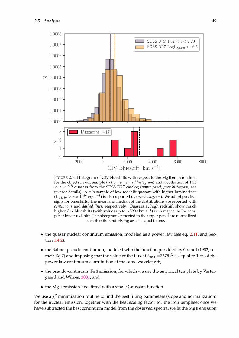
2.5. Analysis 49
0.0000
0.0001
0.0002
0.0003
0.0004
0.0005
0.0006
0.0007
0.0008
NSDSS DR7 1.52 < z < 2.20
SDSS DR7 LogLλ,1350 > 46.5
−2000 0 2000 4000 6000 8000
CIV Blueshift [km s−1]
0
1
2
3
N
Mazzucchelli+17
FIGURE 2.7: Histogram of C IV blueshifts with respect to the Mg II emission line,for the objects in our sample (bottom panel, red histogram) and a collection of 1.52< z < 2.2 quasars from the SDSS DR7 catalog (upper panel, grey histogram; seetext for details). A sub-sample of low redshift quasars with higher luminosities(Lλ,1350 > 3× 1046 erg s−1) is also reported (orange histogram). We adopt positivesigns for blueshifts. The mean and median of the distributions are reported withcontinuous and dashed lines, respectively. Quasars at high redshift show muchhigher C IV blueshifts (with values up to ∼5900 km s−1) with respect to the sam-ple at lower redshift. The histograms reported in the upper panel are normalized
such that the underlying area is equal to one.
• the quasar nuclear continuum emission, modeled as a power law (see eq. 2.11, and Sec-tion 1.4.2);
• the Balmer pseudo-continuum, modeled with the function provided by Grandi (1982; seetheir Eq 7) and imposing that the value of the flux at λrest =3675 Å is equal to 10% of thepower law continuum contribution at the same wavelength;
• the pseudo-continuum Fe II emission, for which we use the empirical template by Vester-gaard and Wilkes, 2001; and
• the Mg II emission line, fitted with a single Gaussian function.
We use a χ2 minimization routine to find the best fitting parameters (slope and normalization)for the nuclear emission, together with the best scaling factor for the iron template; once wehave subtracted the best continuum model from the observed spectra, we fit the Mg II emission

50 Chapter 2. Physical Properties of 15 Quasars at z & 6.5
−2000 0 2000 4000 6000 8000
CIV Blueshift [km s−1]
0.8
1.0
1.2
1.4
1.6
1.8
2.0
2.2L
ogC
IVE
W[A
]SDSS 1.52 < z < 2.20
Mazzucchelli+17
6.5
6.6
6.7
6.8
6.9
7.0
Red
shif
t
FIGURE 2.8: Rest frame C IV EW as a function of C IV blueshift, for the quasarsin our sample (big squares color-coded with respect to redshifts) and a sample ofquasars at lower redshift from SDSS DR7 (Shen et al. 2011; grey points and blackcontours; see text for details on the definition of this sub-sample). Quasars atlow−redshift with very high blueshifts have small EW. The high redshift quasarsare characterized by extreme blueshifts and small C IV EW, following the trend at
z ∼ 1 but with larger scatter.
line (see for further details Decarli et al. 2010). We apply this routine to all the quasars withNIR information in our sample. We exclude PSO183+05 from this analysis, since this source isa weak emission line quasar (see Figure 2.3) and the Mg II fit is highly uncertain.
We show the obtained fit for the 11 remaining objects in Figure 2.9. In Table 2.7, we listthe derived monochromatic luminosities at rest-frame λrest =3000 (λL3000), calculated from thecontinuum flux (Fλ,3000); the properties of the Mg II line (FWHM and flux); the flux of the Fe II
emission and the redshift estimates zMg II. We consider the 14th and 86th interquartiles of theχ2 distribution as our 1σ confidence levels.
De Rosa et al., 2014 applied a similar analysis to the spectra of ULAS1120, VIK0305, VIK0109,VIK2348; their fitting procedures is however slightly different, since they fit all the spectralcomponents at once, using the entire spectral range. Also, Venemans et al., 2015b analyzed theNIR spectra of PSO036+03, PSO338+29 and PSO167-13, considering solely the nuclear contin-uum emission fitted with a power law and modeling the Mg II emission line with a Gaussianfunction. The estimates that both studies obtain for zMg II, black hole masses and bolometricluminosities are consistent, within the uncertainties, with the ones found here (see also Section2.5.6 and Table 2.8).

2.5.A
nalysis51
TABLE 2.7: Quantities derived from the fit of the spectral region around the Mg II emission line: the monochromatic luminosity atrest-frame wavelength 3000 Å (λL3000); FWHM, flux and redshift estimates of the Mg II line, and the Fe II flux.
Name λL3000 MgII FWHM MgII Flux FeII Flux zMg II[1046erg s−1] [km s−1] [10−17erg s−1 cm−2] [10−17erg s−1 cm−2]
VIK J0109–3047 1.0+0.1−0.8 4313+606
−560 22.5+6.8−6.2 45+125
−0.15 6.763±0.01PSO J036.5078+03.0498 3.9+0.4
−1.2 4585+691−461 59.4+11.8
−9.2 147+221−81 6.533+0.01
−0.008VIK J0305–3150 1.5+0.2
−0.7 3210+450−293 41.0+7.2
−5.0 42+124−15 6.610+0.006
−0.005PSO J167.6415–13.4960 0.9+0.3
−0.4 2071+211−354 8.2+1.4
−0.8 <201 6.505±0.005ULAS J1120+0641 3.6+0.4
−1.4 4258+524−395 58.5+9.3
−7.8 61+225−8 7.087+0.007
−0.009HSC J1205–0000 0.7+0.3
−0.4 8841+3410−288 49.8+5.9
−52.4 < 182 6.73+0.01−0.02
PSO J231.6576–20.8335 3.7+0.7−0.9 4686+261
−1800 87.6+9.0−28.2 216+204
−128 6.587+0.012−0.008
PSO J247.2970+24.1277 3.4+0.1−1.5 1975+312
−288 40.2+4.4−5.8 54+234
−0.2 6.476±0.004PSO J323.1382+12.2986 1.6+0.1
−1.0 3923+446−380 45.9+7.4
−7.2 85+109−45 6.592+0.007
−0.006PSO J338.2298+29.5089 0.8+0.4
−0.2 6491+5431105 47.7+7.0
−9.0 76+44−54 6.66+0.02
−0.01VIK J2348–3054 0.9+0.4
−0.3 5444+470−1079 44+8.2
−8.5 95+41−72 6.902±0.01
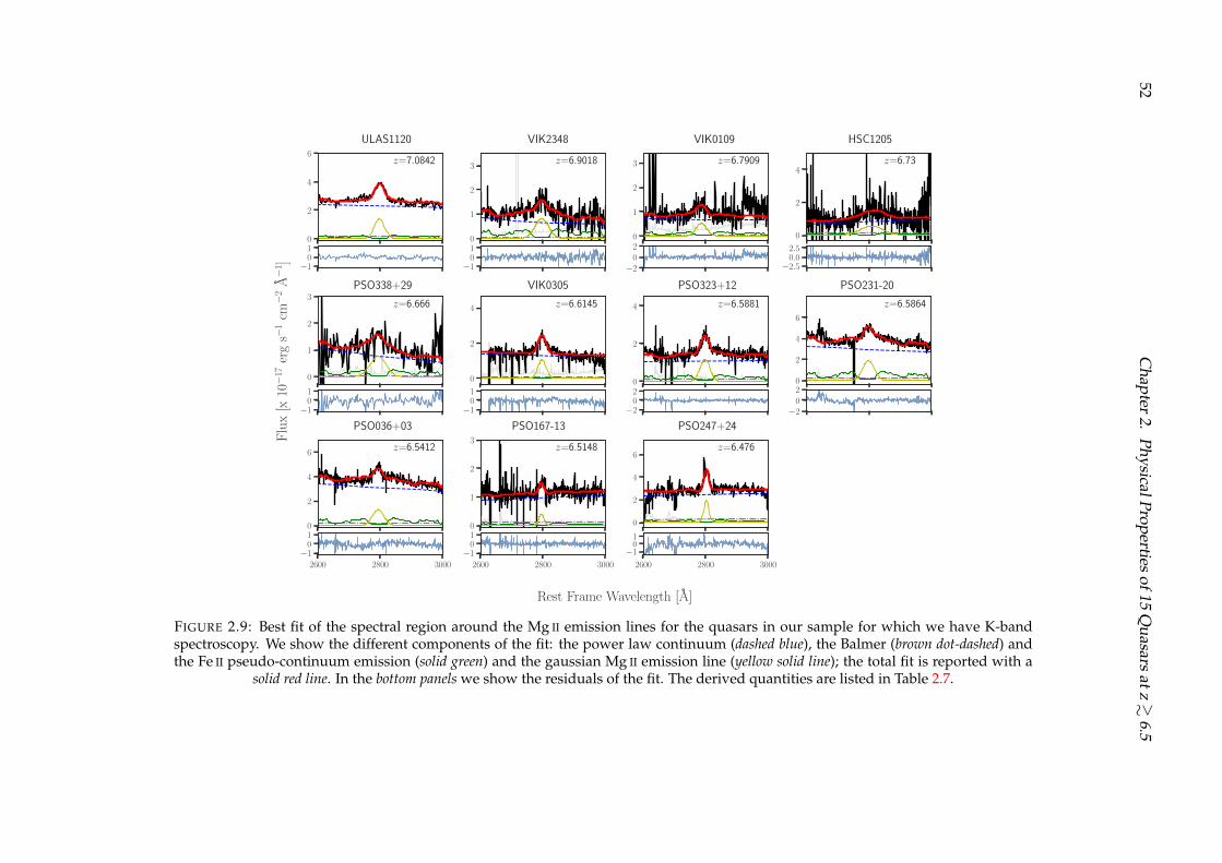
52C
hapter2.
PhysicalPropertiesof15
Quasars
atz&
6.5
0
2
4
6
−101
0
1
2
3
−101
0
1
2
3
−202
0
2
4
−2.50.02.5
0
1
2
3
−101
0
2
4
−101
0
2
4
−202
0
2
4
6
−202
0
2
4
6
2600 2800 3000
−101
0
1
2
3
2600 2800 3000
−101
0
2
4
6
2600 2800 3000
−101
Flu
x[x
10−1
7er
gs−
1cm−2
A−1
]
Rest Frame Wavelength [A]
ULAS1120 VIK2348 VIK0109 HSC1205
z=7.0842 z=6.9018 z=6.7909 z=6.73
PSO338+29 VIK0305 PSO323+12 PSO231-20
z=6.666 z=6.6145 z=6.5881 z=6.5864
PSO036+03 PSO167-13 PSO247+24
z=6.5412 z=6.5148 z=6.476
FIGURE 2.9: Best fit of the spectral region around the Mg II emission lines for the quasars in our sample for which we have K-bandspectroscopy. We show the different components of the fit: the power law continuum (dashed blue), the Balmer (brown dot-dashed) andthe Fe II pseudo-continuum emission (solid green) and the gaussian Mg II emission line (yellow solid line); the total fit is reported with a
solid red line. In the bottom panels we show the residuals of the fit. The derived quantities are listed in Table 2.7.

2.5. Analysis 53
2.5.6 Black Hole Masses
We can estimate the quasar black hole masses (MBH) from our single epoch NIR spectra usingthe broad Mg II emission line, λLλ,3000, and following Vestergaard and Osmer, 2009 (see Section1.4.3 and eq. 1.29). We can also estimate the Eddington luminosity, using eq. 1.25, and theEddington ratio (see Section 1.4.2). We calculate Lbol using the bolometric correction by Shenet al., 2008:
Lbol
erg s−1 = 5.15× λLλ,3000
erg s−1 (2.12)
The obtained values of black hole masses, bolometric luminosities and Eddington ratios for thequasars in our sample are shown in Table 2.8.
We notice that HSC1205, the faintest object in the sample, presents a very broad Mg II emis-sion line: this leads to a high black hole mass (∼5×10⁹ M) and a low Eddington ratio of 0.06.However, HSC1205 is also characterized by a red J −W1 color of 1.97, suggesting that thequasar has a red continuum, due to internal galactic extinction. This could affect our measure-ment of the quasar intrinsic luminosity and therefore we could observe a value of the Edding-ton ratio lower than the intrinsic one. We test this hypothesis by comparing the observed photo-metric information of this source with a suite of quasar spectral models characterized by differ-ent values of internal reddening E(B−V). We obtain these models by applying the reddeninglaw by Calzetti et al., 2000 to the low−redshift quasar spectral template by Selsing et al., 2016,redshifted at z = 6.73 and corrected for the effect of the IGM absorption following Meiksin,2006. We consider the J magnitude provided by Matsuoka et al., 2016, W1 and W2 from WISE(see Table 2.3) and H and K from the VIKING survey (H=21.38±0.21, K=20.77±0.14). A χ2
minimization routine suggests that this quasar has a large E(B−V)=0.3 (see Figure 2.10). Thecorrected λLλ,3000 is 1.62×1046 erg s−1, and the resulting black hole mass and Eddington ratioare 7.22×10⁹ M and 0.09, respectively. Therefore, even taking into account the high internalextinction, HSC1205 is found to host a very massive black hole and to accrete at the lowest ratein our sample.
We now place our estimates in a wider context, comparing them with those derived forlow−redshift quasars. We consider the SDSS-DR7 and DR12 quasar catalogs, presented byShen et al., 2011 and Pâris et al., 2017, respectively; we select only objects in the redshift range0.35 < z < 2.35. In the DR7 release, we take into account the objects with any measurementsof λLλ,3000 and Mg II FWHM (85,507 out of ∼105,000 sources). We calculate λLλ,3000 for thequasars in the DR12 release, modeling a continuum power law with the index provided in thecatalog (entry ALPHA_NU), and normalizing it to the observed SDSS i magnitude. We consideronly the sources in DR12 with measurements of the power law index and of the Mg II FWHM,and not already presented in DR7. Thus, out of the 297,301 sources in DR12, we select 68,062objects: the total number of sources is 153,569.
De Rosa et al., 2011 provide continuum luminosities and Mg II measurements for 22 quasarsat 4.0 . z . 6.4 (observations collected from several studies: Iwamuro et al. 2002, 2004, Barthet al. 2003, Jiang et al. 2007, Kurk et al. 2007, 2009); Willott et al., 2010a present data for ninelower luminosity (Lbol < 1047 erg s−1) z ∼ 6 quasars; finally, Wu et al., 2015 publish an ultraluminous quasar at z ∼ 6.3. In order to implement a consistent comparison among the variousdata sets, we re-calculate the black hole masses for all the objects in the literature using eq. 1.29.In Figure 2.11 we show MBH vs Lbol, for the quasars presented here and the objects from the

54 Chapter 2. Physical Properties of 15 Quasars at z & 6.5
1 2 3 4 5 6
Observed Wavelength [µm]
0.00
0.05
0.10
0.15
0.20
0.25
0.30
0.35
0.40
Flu
xD
ensi
ty[1
0−17
erg
s−1
cm−2
A−1
]
HSC1205E(B-V)=0.3
Selsing Template
Model Photometry
Observed Photometry
FIGURE 2.10: Fit of the broad band photometry of the quasar HSC1205, at z=6.73.The data are found to be consistent with a quasar model with internal reddening
of E(B−V)=0.3
aforementioned studies. We highlight regions in the parameter space with constant Eddingtonratio of 0.01, 0.1 and 1; we also show the typical errors on the black hole masses, due to themethod uncertainties, and on the bolometric luminosities.
We note that the quasars at z & 4 are generally found at higher bolometric luminosities(Lbol & 1046 erg s−1) than the objects at z ∼ 1 (also due to selection effects, see below), butthat the observed black hole masses span a similar range for both samples (108 . MBH/M .5× 109). The bulk of the low redshift (z ∼ 1) quasar population shows lower Eddington ratiosthan the quasars at z & 4. As for the objects at z > 6.4 presented in this sample, they occupya parameter space similar to the sources from De Rosa et al., 2011, with a larger scatter inbolometric luminosities.
In order to provide a consistent comparison, we study the evolution of the black hole massesand Eddington ratios, as a function of redshift, for a quasar sample matched in bolometric lumi-nosity. In order to reproduce the same luminosity distribution as the one of the high−redshiftsources, we sample the low−redshift SDSS quasars by randomly drawing sources with com-parable Lbol to z & 6.5 quasars (within 0.01dex); we repeat this trial for 1000 times. We show inFigure 2.12 the black hole masses, bolometric luminosities and Eddington ratios, as a functionof redshift, for the quasars presented in this work and for objects in one of the samples drawnat z ∼ 1. The distributions of these quantities are also reported in Figure 2.13. We consider,as representative values for black hole mass and Eddington ratio of a bolometric luminositymatched sample at z ∼1, the mean of the means and the mean of the standard deviations cal-culated from the 1000 sub-samples. We then obtain 〈log(MBH)〉=9.21 and 〈log(Lbol/LEdd)〉=-0.47, with a scatter of 0.34 and 0.33, respectively. These values are consistent, also consider-ing the large scatter, with the estimates obtained for z &6.5 quasars: 〈log(MBH)〉=9.21 and〈log(Lbol/LEdd)〉=-0.41, with a scatter of 0.34 and 0.44, respectively. Therefore, considering abolometric luminosity matched sample, we do not find convincing evidence for an evolutionof quasars accretion rate with redshift.

2.5. Analysis 55
44 45 46 47 48
log Lbol [erg s−1]
7.5
8.0
8.5
9.0
9.5
10.0
10.5
log
MB
H[M]
0.01 Ledd
0.1 Ledd Ledd
SDSS 0.35 < z < 2.25
Willott+10
De Rosa+11
De Rosa+14
Wu+15
Mazzucchelli+17
FIGURE 2.11: Black hole mass as function of bolometric luminosity for severalquasar samples. We report a sub-sample from the SDSS-DR7 and DR12 quasarcatalogs (Shen et al. 2011 and Pâris et al. 2017, respectively) at 0.35 < z < 2.25(grey points and countours). Also, we show measurements for quasars at higherredshifts, from Willott et al. (2010, z ∼ 6; green filled diamonds), De Rosa et al.(2011, 4 < z < 6.4; blue points), Wu et al. (2015, z ∼ 6.3; dark red hexagon). Theobjects presented in this study are reported with red, filled squares. We noticethat four quasars (VIK0109, VIK0305, VIK2348 and ULAS1120) have also beenanalyzed by De Rosa et al. (2014, orange empty diamonds): the two sets of measure-ments are consistent within the error bars. We show the method uncertainties onthe black hole mass estimates and a representative mean error on the bolometricluminosity measurements (black point), and regions in the parameter space withconstant Eddington luminosity (black lines). Quasars at high redshift are generallycharacterized by higher Eddington ratios than their lower−redshift counterparts,suggesting that they accreate at higher rates. However, the scatter in the z & 6.5
sample is not negligible, with objects at Lbol/LEdd as low as ∼0.1.

56 Chapter 2. Physical Properties of 15 Quasars at z & 6.5
0 1 2 3 4 5 6 7
8.0
8.5
9.0
9.5
10.0
10.5
11.0
log
MB
H[M]
SDSS 0.35 < z < 2.25 Mazzucchelli+17
0 1 2 3 4 5 6 7
−1.5
−1.0
−0.5
0.0
0.5
1.0
logL
bol/L
Ed
d
0 1 2 3 4 5 6 7
Redshift
46.4
46.6
46.8
47.0
47.2
47.4
47.6
logL
bol
[erg
s−1 ]
FIGURE 2.12: Black hole mass (upper), Eddington ratio (central) and bolomet-ric luminosity (lower panel) against redshift, for a bolometric luminosity matchedquasar sample (see text for details on the selection of the subsample at z ∼1).We report the z &6.5 quasars presented in this work with red squares, and theones at lower redshift (0.35 < z < 2.25) from SDSS-DR7+DR12 (Shen et al. 2011,Pâris et al. 2017) with grey points, respectively. The mean values of quasars blackhole masses and Eddington ratios do not vary significantly with redshift (see also
Figure 2.13).
Finally, we caution that we have witnessed evidence suggesting the presence of a strongwind component in the BLR (see Sections 2.5.4 and 2.5.1). In case of non-negligible radiationpressure by ionizing photons acting on the BLRs, the black hole masses derived by the simpleapplication of the virial theorem might be underestimated (e.g. Marconi et al. 2008). This effectdepends strongly on the column density (NH) of the BLR, and on the Eddington ratio. Marconiet al., 2008 show that, in case of 0.1. Lbol/LEdd .1.0, as found in z &6.5 quasars, and for typicalvalues of 1023 < NH/[cm−2] <1024, the true black hole masses would be ∼2-10× larger thanthe virial estimates. This would lead to an even stronger challenge for the current models ofprimordial black holes formation and growth. An in depth discussion of this effect, given theuncertainties on the contribution of the possible wind and on the BLR structure itself, is beyondthe scope of this work.

2.5.A
nalysis57
8 9 10 11log MBH [M]
0
1
2
3
4
5
N
SDSS 0.35 < z < 2.25
Mazzucchelli+17
−2 −1 0 1log Lbol/LEdd
46.50 46.75 47.00 47.25 47.50log Lbol [erg s−1]
FIGURE 2.13: Distribution of black hole masses (left), Eddington ratios (central) and bolometric luminosities (right panel) for one of the1000 bolometric luminosity matched sub-samples drawn from low−redshift SDSS quasars (grey histograms; Shen et al. 2011 and Pâriset al. 2017; see text for details), and for the z & 6.5 quasars presented here (red histograms). The grey points represent the mean of blackhole masses, Eddington ratios and bolometric luminosities in each bin, resulting from all the 1000 trials at z ∼1. The mean of eachquantity, for the low and high redshift populations, are shown in each panel with black and red dashed lines, respectively. We note thatthe mean black hole masses and Eddington ratios of the two samples are consistent, suggesting a non evolution of accretion rate with
cosmic time. The histograms are normalized such that the underlying area is equal to one.

58 Chapter 2. Physical Properties of 15 Quasars at z & 6.5
2.5.7 Black Hole Seeds
Measurements of black hole masses and Eddington ratios of high−redshift quasars help us inconstraining formation scenarios of the first supermassive black holes in the very early uni-verse. From eq. 1.30, we can derive that the time in which a black hole of mass MBH,f is grownfrom an initial seed MBH,seed, assuming it accretes with a constant Eddington ratio for all thetime, can be written as (see also,e.g. Shapiro 2005, Volonteri and Rees 2005):
tGyr
= ts ×[
ε
1− ε
]× LEdd
Lbol× ln
(MBH,f
MBH,seed
)(2.13)
The average MBH and Lbol/LEdd of all the z & 6.5 quasars in the sample presented here (11 ob-jects, not considering any luminosity cut, see Table 2.8) are 1.62×10⁹ M and 0.39, respectively.If we insert these values in Eq. 2.13, we can calculate the time needed by a black hole seed ofMBH,seed = [102, 104, 105, 106] M to grow to the mean MBH found here, assuming that it alwaysaccretes at an average Eddington rate of ∼0.39. We find that this time is t =[1.44,1.04,0.84,0.64]Gyr. As the age of the universe at z∼6.5 is only ∼0.83 Gyr (see Section 1.1), this implies thatonly very massive seeds (∼106 M) would be able to form the observed supermassive blackholes.
Alternatively, we can invert eq. 2.13 and derive the initial masses of the black hole seedsrequired to obtain the observed black holes. This result depends on the assumptions made, e.g.,on the redshift of the seed formation (zi), on the accretion rate (Lbol/LEdd), and on the radiativeefficiency (ε; see eq. 2.13)13. We here consider different values for these parameters: We assumethat the black holes accrete constantly with the observed Eddington ratios or with Lbol/LEdd=1;also, we consider that they grow for a period of time equal to the age of the universe at theirredshifts (i.e. zi → ∞), and from zi=30 or 20. Finally, we assume an efficiency of 7% or 10%.The derived values of black hole seeds for all the combinations of these parameters are shownin Figure 2.14.
In all the cases considered here with ε=0.07 and Eddington accretion (and in case of ε=0.1,zi → ∞ and Lbol/LEdd=1), the calculated seed masses (&102 M) are consistent with beingformed by stellar remnants. Alternatively, a scenario of higher efficiency (ε=0.1), later seedsbirth (i.e. z =30 or 20), and accretion at Lbol/LEdd=1, would require more massive seeds (∼103−4
M) as progenitors of the observed z &6.5 quasars.
2.5.8 Fe II/ Mg II
The estimates of the relative abundances of metals in high redshift sources act as useful proxiesin the investigation of the chemical composition and evolution of galaxies in the early universe.In this context, the Mg II/Fe II ratio is of particular interest: α-elements, such as Mg, are mainly
13The efficiency depends in turn on the black hole spin and can be as high as ∼40% in the case of maximallyspinning black holes. The spin is still an elusive parameter; it has been observationally measured only in ∼20sources in the local Universe (through the relativistic broadening of the Fe Kα line; Brenneman et al. 2011 andReynolds 2014). Thanks to stacked Chandra deep observations of ∼30 lensed quasars Walton et al., 2015 detecteda broadened component of the Kα line up to z ∼4.5; however the low S/N prevented a measurement of the singlequasars’ black hole spins. Current semi-analytical models place only weak constraints on the spin value at z &5,which depends on the gas accretion mode, galactic morphology and black hole mass (e.g. Sesana et al. 2014).However, since the spin decreases with black hole mass, we do not expect large values for our sample of quasarswith MBH &108 M.

2.5. Analysis 59
TABLE 2.8: Estimated quantities for the quasars in our sample: bolometric lumi-nosities, black hole masses, Eddington ratios, Fe II-to-Mg II flux ratios.
Name Lbol MBH Lbol/LEdd Fe II/Mg II[1047erg s−1] [×109M ]
VIK J0109–3047 0.51+0.05−0.06 1.33+0.38
−0.62 0.29+0.88−2.59 2.02+5.56
−0.65PSO J036.5078+03.0498 2.0+0.22
−0.64 3.00+0.92−0.77 0.51+0.17
−0.21 2.47+3.71−1.36
VIK J0305–3150 0.75+0.10−0.34 0.90+0.29
−0.27 0.64+2.20−3.42 1.03+3.04
−0.37PSO J167.6415–13.4960 0.47+0.16
−0.22 0.30+0.08−0.12 1.22+0.51
−0.75 <3.1ULAS J1120+0641 1.83+0.19
−0.072 2.47+0.62−0.67 0.570.16
0.27 1.04+3.84−0.14
HSC J1205–0000 0.36+0.18−0.20 4.7+1.2
−3.9 0.06+0.32−0.58 <0.50
PSO J231.6576–20.8335 1.89+0.34−0.45 3.05+0.44
−2.24 0.48+0.11−0.39 2.64±1.7
PSO J247.2970+24.1277 1.77+0.06−0.76 0.52+0.22
−0.25 2.60+0.08−0.15 1.33+5.82
−0.01PSO J323.1382+12.2986 0.81+0.07
−0.50 1.39+0.32−0.51 0.44+1.09
−3.19 1.85+2.37−0.97
PSO J338.2298+29.5089 4.04+2.14−0.90 2.70+0.85
−0.97 0.11+0.71−0.49 1.29+2.1
−0.74VIK J2348–3054 0.43+0.20
−0.13 1.98+0.57−0.84 0.17+0.92
−0.88 2.13+0.93−1.54
produced via type II supernovae (SNe) involving massive stars, while type Ia SNe from binarysystems are primarily responsible for the provision of iron (Nomoto et al., 1997). Given thatSNe Ia are expected to be delayed by∼1 Gyr (Matteucci and Greggio 1986) with respect to typeII SNe, estimating the relative abundances of α-elements to iron provides important insightson the stellar population in the galaxy, and on the duration and intensity of the star forma-tion burst. Tracking the evolution of the Mg II/Fe II ratio as a function of redshift allows us toreconstruct the evolution of the galactic star formation history over cosmic time.
Many studies in the literature investigate the Mg II/Fe II ratio in the BLR of quasars, byestimating the ratio of the Fe II and Mg II fluxes (FFe II/FMg II), considered a first-order proxy ofthe abundance ratio (e.g. Barth et al. 2003, Maiolino et al. 2003, Iwamuro et al. 2002,2004, Jianget al. 2007, Kurk et al. 2007, Sameshima et al. 2009, De Rosa et al. 2011,2014). In particular, DeRosa et al., 2011 and 2014 present a consistent analysis of ∼30 quasar spectra in the redshiftrange 4 . z . 7.1, and find no evolution of their FFe II/FMg II with cosmic time.
We estimate the Fe II and Mg II fluxes for the quasars in our study following De Rosa etal., 2014: for the former we integrate the fitted iron template over the rest-frame wavelengthrange 2200 < λ/ [Å] < 3090, and for the latter we compute the integral of the fitted Gaussianfunction (see Table 2.7 and 2.8 for the estimated flux values). In Figure 2.15, we plot FFe II/FMg II
as a function of redshift, for both the quasars in our sample and sources from the literature. Weconsider the sample by De Rosa et al., 2011 and 2014, and a sample of low−redshift quasars(z . 2.05) from Calderone et al., 2017. They consistently re-analyzed a sub-sample of quasars(∼70,000) from the SDSS-DR10 catalog, and provide measurements of the flux for Mg, Fe andthe continuum emission at rest-frame λrest =3000 Å14. Here, we take only the sources with noflag on the quantities above (∼44,000 objects), and we correct the Fe II flux to account for thedifferent wavelength ranges where the iron emission was computed15.
14http://qsfit.inaf.it/15Calderone et al., 2017 integrates the iron template in the rest-frame wavelength range 2140 < λ/[Å] < 3090,
while we use the range 2200 < λ/[Å] < 3090.
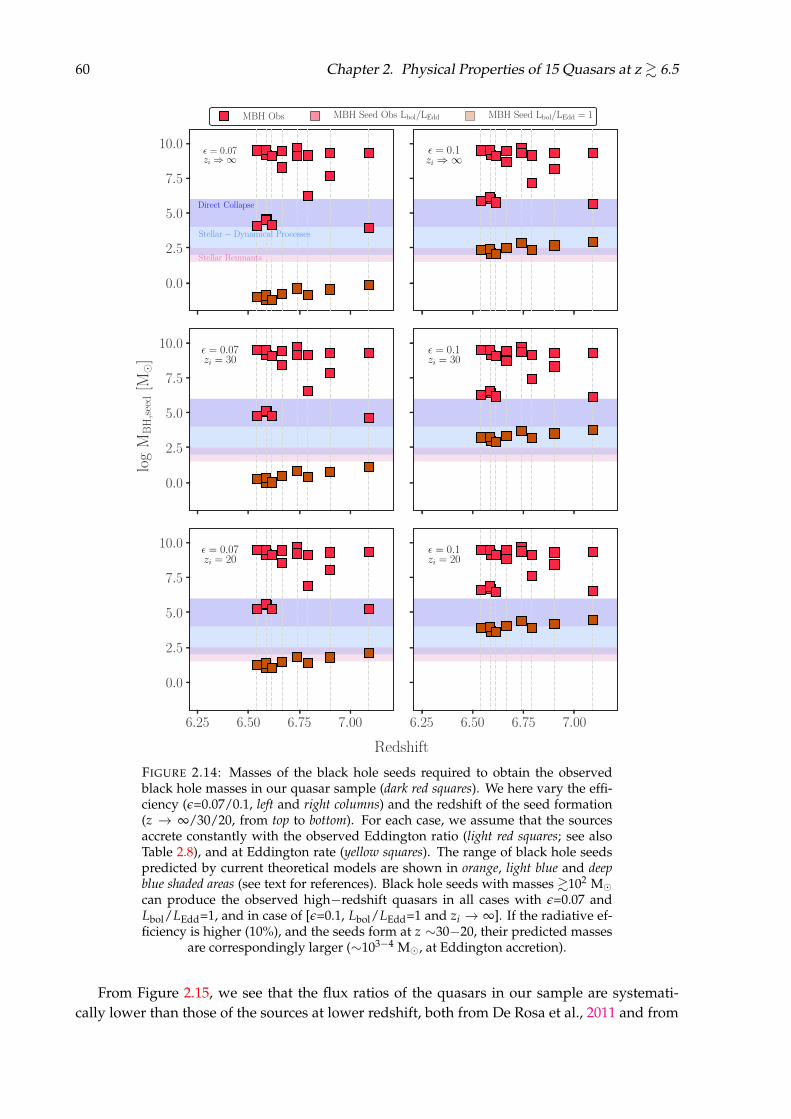
60 Chapter 2. Physical Properties of 15 Quasars at z & 6.5
0.0
2.5
5.0
7.5
10.0ε = 0.07zi ⇒∞
Direct Collapse
Stellar− Dynamical Processes
Stellar Remnants
MBH Obs MBH Seed Obs Lbol/LEdd MBH Seed Lbol/LEdd = 1
ε = 0.1zi ⇒∞
0.0
2.5
5.0
7.5
10.0 ε = 0.07zi = 30
ε = 0.1zi = 30
6.25 6.50 6.75 7.00
0.0
2.5
5.0
7.5
10.0 ε = 0.07zi = 20
6.25 6.50 6.75 7.00
ε = 0.1zi = 20
log
MB
H,s
eed
[M]
Redshift
FIGURE 2.14: Masses of the black hole seeds required to obtain the observedblack hole masses in our quasar sample (dark red squares). We here vary the effi-ciency (ε=0.07/0.1, left and right columns) and the redshift of the seed formation(z → ∞/30/20, from top to bottom). For each case, we assume that the sourcesaccrete constantly with the observed Eddington ratio (light red squares; see alsoTable 2.8), and at Eddington rate (yellow squares). The range of black hole seedspredicted by current theoretical models are shown in orange, light blue and deepblue shaded areas (see text for references). Black hole seeds with masses &102 Mcan produce the observed high−redshift quasars in all cases with ε=0.07 andLbol/LEdd=1, and in case of [ε=0.1, Lbol/LEdd=1 and zi → ∞]. If the radiative ef-ficiency is higher (10%), and the seeds form at z ∼30−20, their predicted masses
are correspondingly larger (∼103−4 M, at Eddington accretion).
From Figure 2.15, we see that the flux ratios of the quasars in our sample are systemati-cally lower than those of the sources at lower redshift, both from De Rosa et al., 2011 and from

2.5. Analysis 61
Calderone et al., 2017: this suggests a possible depletion of iron at z & 6.5, and therefore thepresence of a younger stellar population in these quasar host galaxies. However, our estimatesare also characterized by large uncertainties, mainly due to the large uncertainties on the ironflux estimates (see Table 2.7). Within the errors, our measurements are consistent with a sce-nario of non−evolving FFe II/FMg II over cosmic time, in agreement with De Rosa et al., 2014.
We test whether the systematic lower values of FFe II/FMg II for the highest redshift quasarpopulation is statistically significant. We associate to each of our measurements a probabilitydistribution, built by connecting two half-Gaussian functions with mean and sigma equal to thecalculated ratio and to the lower (or upper) uncertainty, respectively. We sum these functionsto obtain the total probability distribution for the objects at high−redshift. We compare thisfunction with the distribution of the FFe II/FMg II values for the quasars at z ∼ 1. We randomlydraw nine sources from the two distributions (the number of objects in our sample excludingthe limits) and we apply a Kolmogorov-Smirnoff test to check if these two samples could havebeen taken from the same probability distribution; we repeat this draw 10000 times. We obtainthat the p-value is greater than 0.2 (0.5) in the 51% (27%) of the cases: this highlights that,considering the large uncertainties, we do not significantly measure a difference in the totalprobability distribution of FFe II/FMg II at low and high−redshift.
Data with higher S/N in the Fe II emission line region are needed to place more stringentconstraints on the evolution of the abundance ratio.
2.5.9 Infrared and [CII] luminosities in Quasar Host Galaxies
We observed four quasars in our sample with NOEMA (see Section 2.3). We extract their spec-tra, and fit the continuum+[CII] line emission with a flat+Gaussian function (see Figure 2.4).We estimate the line properties, e.g. the peak frequency, the width, amplitude and flux, and wecalculate the continuum flux at rest frame wavelength 158 µm from the continuum map. Wereport these values in Table 2.9.
We can derive the far infrared properties of the observed quasars, following a numberof assumptions commonly presented in the literature (e.g. Venemans et al. 2012, 2016). Weapproximate the shape of the quasar infrared emission with a modified black body: fν ∝Bν(Td)(1− eτd), where Bν(Td) is the Planck function and Td and τd are the dust temperatureand optical depth, respectively (Beelen et al., 2006). Under the assumption that the dust is op-tically thin at wavelength λrest > 40µm (τd << 1), we can further simplify the function aboveas fν ∝ Bν(Td)ν
β, with β the dust emissivity power law spectral index. We take Td = 47 Kand β = 1.6, which are typical values assumed in the literature (Beelen et al., 2006). We scalethe modified black body function to the observed continuum flux at the rest frame frequencyνrest = 1900 GHz; we then calculate the FIR luminosity (LFIR) integrating the template in therest frame wavelength range 42.5 µm−122.5µm (Helou et al., 1988). The total infrared (TIR) lu-minosity (LTIR) is defined instead as the integral of the same function from 8 µm to 1000 µm. Wenote that these luminosity values are crucially dependent on the assumed shape of the quasarinfrared emission. We can use the latter quantity to derive the star formation rate (SFRTIR) of

62 Chapter 2. Physical Properties of 15 Quasars at z & 6.5
0 1 2 3 4 5 6 7
Redshift
0
2
4
6
8F
FeI
I/F
Mg I
I
SDSS QSOs z < 2.0
De Rosa+11
De Rosa+14
Mazzucchelli+17
FIGURE 2.15: Fe II-to-Mg II flux ratio, considered as a first-order proxy for the rel-ative abundance ratio, versus redshift. We show the quasars in our sample (redsquares and, in case of upper limits, down-pointing triangles) and taken from theliterature: De Rosa et al. 2011 (blue points) and z . 2 SDSS quasars (Calderone etal. 2017, grey points and black contours). We show with orange empty diamonds themeasurements of De Rosa et al., 2014 for four of our quasars (VIK0109, VIK0305,VIK2348 and ULAS1120); they have been derived with a slightly different fittingroutine (see text for details) but are consistent, within the errors, with the esti-mates obtained here. Our measurements are systematically lower than that ofsamples at lower redshifts; however, taking into account the large uncertainties,
we find no statistical evidence for an evolution of the flux ratio with redshift.
the quasar host galaxy, through the relation calibrated by Murphy et al., 2011:
SFR[M yr−1]
= 3.88× 10−44 LTIR
[erg s−1](2.14)
Finally, we can estimate the total dust mass as (Magdis et al., 2011):
Md =fνD2
L(1 + z) κλBν(λ, Td)
(2.15)
where DL is the luminosity distance, Bν(λ, Td) and fν are the Planck function and continuumflux density, respectively, estimated at λrest. κλ is the dust mass opacity coefficient, which canbe expressed as κλ = 0.77 (850µm/λ)β cm2/g (Dunne, Clements, and Eales, 2000).
We can also calculate the luminosity of the [CII] emission line (L[CII]) from the observed lineflux (S[CII]∆v; Carilli and Walter 2013):
L[CII]
L= 1.04× 10⁻³ S[CII] ∆v
Jy km s−1
(DL
Mpc
)2 νobs
GHz(2.16)

2.5. Analysis 63
where νobs is the observed frequency. Several studies in the literature find a correlation be-tween L[CII] and the SFR, and providing different recipes to derive SFR[CII] , which have beencalibrated on a variety of data sets (De Looze et al. 2011, 2014, Sargsyan et al. 2012a, Herrera-Camus et al. 2015). We consider here the formula obtained by De Looze et al. 2014, who used asample of high redshift (z > 0.5) galaxies:
SFR[CII]
[M yr−1]= 3× 10⁻⁹
(L[CII]
L
)1.18
(2.17)
The observed scatter of this relation is ∼0.40 dex. We note that, using the relations from DeLooze et al., 2011 (Herrera-Camus et al., 2015), calibrated on local star forming galaxies, weobtain values of the SFR[CII] ∼ ×2 (5) lower. This difference may be due to the diverse lumi-nosity range of the sources analyzed in this study (LFIR & 1012 M) and the ones considered inthe literature (LFIR < 1012 M; see also the discussion in Venemans et al. 2016). In Table 2.9, welist our estimates for the [CII] , FIR and TIR luminosities, SFRTIR, SFR[CII] and dust masses.
In Figure 2.16, we plot L[CII] /LFIR vs LFIR for the quasars studied here and for a variety ofsources from the literature. At low redshift (z < 1) both star-forming galaxies (Malhotra et al.2001, Sargsyan et al. 2012a) and more extreme objects, e.g. LIRGS and ULIRGS (Díaz-Santoset al. 2013, Farrah et al. 2013), show lower luminosity ratios at higher FIR luminosities: thisphenomenon is known as the “CII-deficit”. At z > 1, the scenario is less clear, where the scatterin the measurements of L[CII] /LFIR for star-forming galaxies (Stacey et al. 2010, Brisbin et al.2015, Gullberg et al. 2015), SMGs and quasars increases.
Quasars at z > 5 present a variety of L[CII] /LFIR values, mostly depending on their far-infrared brightness. Walter et al., 2009 and Wang et al., 2013 observe quasars with high LFIR,and show that they are characterized by low luminosity ratios, comparable to local ULIRGS(〈log(L[CII] /LFIR)〉 ∼ −3.5). On the other hand, quasars with lower far infrared luminositiesand black hole masses (MBH < 109 M ; Willott, Bergeron, and Omont 2015) are located in a re-gion of the parameter space similar to that of regular star forming galaxies (〈log(L[CII] /LFIR)〉 ∼−2.5). In the literature, the decrease of L[CII] in high-redshift quasars has been tentatively ex-plained invoking a role of the central AGN emission, which is heating the dust. The problemis however still under debate, and several other alternative scenarios have been advocated,e.g. C+ suppression due to X-ray radiation from the AGN (Langer and Pineda, 2015), or the rel-ative importance of different modes of star formation on-going in the galaxies (Graciá-Carpioet al., 2011).
The quasars whose new infrared observations are presented here, with LFIR ∼ 1012 L, arecharacterized by values of the luminosity ratio in between those of FIR bright quasars and ofthe sample by Willott, Bergeron, and Omont (2015; 〈log(L[CII] /LFIR)〉 ∼ −3.0). This is similarto what was found by Venemans et al. (2012, 2017) for ULAS1120, and suggests that the hostgalaxies of these quasars are more similar to ULIRGS.

64C
hapter2.
PhysicalPropertiesof15
Quasars
atz&
6.5
TABLE 2.9: Results from our NOEMA observations: we report the [CII] line and continuum emission quantities obtained from our fit(i.e. flux and line width); the [CII] line, FIR and TIR luminosities; the [CII] and TIR SFR, and the dust masses.
HSC J1205-0000 PSO J338.2298+29.5089 PSO J006.1240+39.2219 PSO J323.1283+12.2986
z[CII] − zMgII [km s−1] − 818+168−138 − 230 ± 13
[CII] line width [km s−1] − 740+541−313 277+161
−141 254+48−28
[CII] flux [Jy km s−1] − 1.72+0.91−0.84 0.78+0.54
−0.38 1.05+0.33−0.21
Continuum flux density [mJy] 0.833 ± 0.176 0.972 ± 0.215 0.548 ± 0.178 0.470 ± 0.146L[CII] [× 109 L] − 2.0 ± 0.1 0.9+0.6
−0.4 1.2+0.4−0.2
LFIR [× 1012 L] 1.9 ± 0.4 2.1 ± 0.5 1.1 ± 0.4 1.0 ± 0.3LTIR [× 1012 L] 2.6 ± 0.5 2.8 ± 0.6 1.5 ± 0.5 1.3 ± 0.4L[CII] /LFIR [× 10−3] − 0.98+0.55
−0.52 0.77+0.59−0.45 1.2+0.54
−0.45SFRTIR [M yr−1] 381 ± 76 413 ± 91 231 ± 75 196 ± 61SFR[CII] [M yr−1] – 285+175
−138 108+89−62 153+57
36Md [× 108 M] 2.6 ± 0.5 2.7 ± 0.6 1.5 ± 0.5 1.3 ± 0.4

2.5. Analysis 65
8 9 10 11 12 13 14 15
log LFIR [L]
−4.0
−3.5
−3.0
−2.5
−2.0
−1.5
−1.0lo
gL
CII/L
FIR
z < 1 z > 1 z > 5
Farrah+13
Sargsyan+14
Diaz-Santos+13
Malhotra+01
Stacey+10
Brisbin+15
Gullberg+15
SMGs/QSOs
Riechers+13
QSOs z < 6.5
QSOs z > 6.5
Mazzucchelli+17
FIGURE 2.16: [CII] -to-FIR luminosity ratio as function of FIR luminosity. Withopen blue/green symbols we report objects at z < 1: star-forming galaxies (Mal-hotra et al. 2001, Sargsyan et al. 2012a), LIRGs (Díaz-Santos et al., 2013) andULIRGS (Farrah et al., 2013). Values for sources at 1 < z < 5 are shown withopen yellow/orange symbols: star-forming galaxies (Stacey et al. 2010, Brisbin et al.2015, Gullberg et al. 2015) and a collection of 3 . z . 5 sub-millimeter galax-ies and quasars (Cox et al. 2011,Wagg et al. 2010, 2012, Ivison et al. 2010, DeBreuck et al. 2011, Valtchanov et al. 2011, Walter et al. 2012, Maiolino et al. 2009).The z = 6.3 SMG presented in Riechers et al., 2013 is shown as a light-red star.Quasars at 5 . z . 6.5 (Maiolino et al. 2005, Wang et al. 2013, Willott, Berg-eron, and Omont 2015) are shown with filled dark-pink diamonds. Quasars in thesample presented here are reported with filled light-pink squares (new observa-tions for PSO338+29, PSO323+12, PSO006+39), and with filled pink circles (datataken from the literature; ULASJ1120, Venemans et al. 2012; PSO036+03, Baña-dos et al. 2015b; VIKJ0109, VIKJ0305, VIKJ2348, Venemans et al. 2016; PSO231-20,PSO183+05,PSO167-13, Decarli et al. 2018). Local sources show a decrease in the[CII] -to-FIR ratio at high FIR luminosities, whereas the values of this ratio for thehigh redshift sample have a large scatter. The z > 6 quasars whose mm observa-tions are presented in this work are characterized by values of L[CII] /LFIR com-parable to local ULIRGs. The range of [CII] -to-FIR luminosity ratio of the generalpopulation of z > 6 quasars however hints to an intrinsic diversity among their
host galaxies.

66 Chapter 2. Physical Properties of 15 Quasars at z & 6.5
2.5.10 Near Zones
Near zones are regions surrounding quasars where the IGM is ionized by the UV radiationemitted from the central source (see Section 1.5). Taking into account several approximations,e.g. that the IGM is partially ionized and solely composed of hydrogen, and that photoioniza-tion recombination equilibrium is found outside the ionized region (Fan et al., 2006), the radiusof the ionized bubble can be expressed as:
Rs ∝(
NQtQ
fHI
)1/3
(2.18)
where NQ is the rate of ionizing photons produced by the quasar, tQ is the quasar lifetime, andfHI is the IGM neutral fraction.
Several studies provide estimates of near zone radii for samples of z > 5 quasars, andinvestigate its evolution as a function of redshift, in order to investigate the IGM evolution(Fan et al. 2006, Carilli et al. 2010, Venemans et al. 2015b, Eilers et al. 2017; see Section 1.5.4).However, it is not straightforward to derive the exact values of Rs from the observed spectra;instead, we calculate here the near zone radii (RNZ) for the sources in our sample. We followthe definition of Fan et al., 2006, i.e. RNZ is the distance from the central source where thetransmitted flux drops below 0.1, once the spectrum has been smoothed to a resolution of 20 Å.The transmitted flux is obtained by dividing the observed spectrum by a model of the intrinsicemission.
We here model the quasar emission at λrest < 1215.16 Å using a principal component anal-ysis (PCA) approach. In short, the total spectrum, q(λ), is represented as the sum of a meanspectrum, µ(λ), and n = 1, .., N principal component spectra (PCS), ξn(λ), each weighted by acoefficient wn:
q(λ) = µ(λ) +N
∑n=1
wnξn(λ) (2.19)
Pâris et al., 2011 and Suzuki, 2006 apply the PCA to a collection of 78 z ∼ 3 and 50 z . 1 quasarsfrom SDSS, respectively. In our study, we follow the approach by Eilers et al., 2017, mainlyreferring to Pâris et al., 2011 who provide PCS functions within the rest frame wavelengthwindow 1020 < λ/[Å] < 2000. After normalizing our spectra to the flux at λrest = 1280 Å,we fit the region redwards than the Lyα emission line (λrest > 1215.16 Å) to the PCS by Pâriset al., 2011, and we derive the best coefficients by finding the maximum likelihood. We thenobtain the best coefficients which reproduce the entire spectrum by using the projection matrixpresented by Pâris et al., 2011. For further details on this modeling procedure, see Eilers et al.,2017. We show in Figure 2.17 an example of PCA for one of the quasars in our sample. Also,in this way we provide an analysis of the near zone sizes consistent with Eilers et al., 2017,making it possible to coherently compare the results obtained from the two data sets.
The near zone sizes depend also on quasar luminosity (through the NQ term in eq. 2.18):if we want to study their evolution with redshift, we need to break this degeneracy. We re-scale the quasar luminosities to the common value of M1450=-27 (following previous studies,e.g Carilli et al. 2010, Venemans et al. 2015b), and we use the scaling relation obtained from themost recent numerical simulations presented in Eilers et al., 2017 and Davies et al., 2018. They

2.5. Analysis 67
1000 1100 1200 1300 1400 1500 1600 1700
Rest Frame Wavelength
0
1
2
3
4
5
6
7
8
Nor
mal
ized
Flu
x
Projected spectral model
Fitted model 8 PCS
PSOJ323.1382+12.2986
FIGURE 2.17: Example of quasar continuum emission fit with the PCA methodfor one of the sources in our sample (PSO323+12). We show the fitted model atwavelength greater than the Lyα emission line (with 8 PCAs; green line), and the
projected model on the entire spectrum (purple line).
simulate radiative transfer outputs for a suite of z =6 quasars within the luminosity range -24.78<M1450 <-29.14, and constantly shining over 107.5 yr, considering two scenarios in whichthe surrounding IGM is mostly ionized (see Sections 1.5 and 1.2; e.g. McGreer, Mesinger, andD’Odorico 2015) or mostly neutral. They obtain comparable results for the two cases, whichare both in agreement with the outcome obtained by fitting the observational data (see Eilerset al. 2017, Figure 5). Following the approach of Eilers et al., 2017, we consider the case of amostly ionized IGM: they fit the simulated quasar near zone sizes against luminosity with thepower law:
RNZ = 5.57 pMpc× 100.4(M1450)/2.35 (2.20)
from which they derive the following scaling relation, that we also use here:
RNZ,corr = RNZ 100.4(27+M1450)/2.35 (2.21)
We report in Table 2.10 the derived quantities, and the transmission fluxes are shown in Figure2.18. We do not consider in our analysis the following quasars: HSC1205, due to the poor qual-ity of the spectrum in the Lyα emission region (see Figure 2.3); PSO183+05, since this quasar isbelieved to present a proximate (z ≈ 6.404) DLA (see Chen et al. 2017, Banados et al. subm);PSO011+09 and PSO261+19. The redshift measurements of these latter two objects are pro-vided by the Lyα emission line: the lack of any other strong emission line, and the broad shapeof the Lyα line, do not permit us to rule out that these quasars are BAL objects. The redshifts ofthe remaining objects are mainly derived from [CII] observations (see Table 2.10).
We show the evolution of RNZ,corr as a function of redshift in Figure 2.19. We compare ourdata with estimates at lower redshift (5.6 . z . 6.6) presented by Eilers et al., 2017. The best fitof the evolution of RNZ,corr with z, modeled as a power law function, gives the following:
RNZ,corr = (4.49± 0.92)×(
1 + z7
)−1.00±0.20
(2.22)

68 Chapter 2. Physical Properties of 15 Quasars at z & 6.5
TABLE 2.10: Near zone sizes of 11 quasars in the sample presented here. Thecorrected vaues have been calculated with Eq. 2.21, and take into account thedependency on their luminosity. We also report the number of PCS adopted in
the continuum fit.
Name RNZ RNZ,corr RNZ,corr,err PCS[Mpc] [Mpc] [Mpc]
PSO J006.1240+39.2219 4.47 6.78 0.09 5VIK J0109–3047 1.59 2.78 0.03 8PSO J036.5078+03.0498 4.37 3.91 0.08 8VIK J0305–3150 3.417 4.81 0.006 10PSO J167.6415–13.4960 2.02 3.55 0.03 8ULAS J1120+0641 2.10 2.48 0.02 9PSO J231.6576–20.8335 4.28 4.05 0.03 8PSO J247.2970+24.1277 2.46 2.96 0.24 5PSO J323.1382+12.2986 6.23 6.09 0.01 8PSO J338.2298+29.5089 5.35 7.68 0.25 5VIK J2348–3054 2.64 4.33 0.05 8
The values obtained are consistent, within the errors, with the results of Eilers et al., 201716. Inagreement with both measurements from observations and radiative transfer simulations pre-sented by Eilers et al., 2017, we find a weak evolution of the quasar near zone sizes with cosmictime: this evolution is indeed much shallower than what was obtained by previous works (Fanet al. 2006, Carilli et al. 2010, Venemans et al. 2015b), which argued that the significant decreaseof RNZ with redshift could be explained by a steeply increasing IGM neutral fraction betweenz ∼5.7 and 6.417.
The different trend of near zone sizes with redshift with respect to what was found in theliterature may be due to several reasons, i.e. we consider higher quality spectra and a largersample of quasars, we take into consideration a consistent definition of RNZ and we do notexclude the WEL quasars at z ∼6 (see Eilers et al. 2017 for an in depth discussion of the dis-crepancies with previous works). We argue that the shallow evolution is due to the fact thatRNZ,corr does not depend entirely or only on the external IGM properties, but it correlates morestrongly with the quasar characteristics (e.g. lifetime, regions of neutral hydrogen within theionized zone), which are highly variable from object to object.
2.6 Discussion and Summary
In this work we present our search for z−dropouts in the third internal release of the Pan-STARRS1 stacked catalog (PS1 PV3), which led to the discovery of six new z ∼6.5 quasars.
We complement these newly found quasars with 9 other z & 6.5 quasars known to date,and perform a comprehensive analysis of the highest redshift quasar population. In particular,we provide new optical/NIR spectroscopic observations for the six newly discovered quasarsand for three sources taken from the literature (PSO006+39, PSO338+29 and HSC1205). We
16RNZ,corr ≈ 4.87× [(1 + z)/7]−1.44; see also their Figure 6.17We note that these studies considered a smaller and lower−z quasar sample, whose redshift measurements
(mainly from the Mg II or Lyα emission lines, with only a minority of objects observed in CO or [CII] ) have larger
errors, and that they fit the redshift evolution of the near zone sizes with a linear relation.

2.6. Discussion and Summary 69
0.0
0.2
0.4
0.6
0.8
1.0
0.0
0.2
0.4
0.6
0.8
1.0
0510
0.0
0.2
0.4
0.6
0.8
1.0
0510 0510
Tra
nsm
issi
on
Proper distance (Mpc)
ULASJ1120 VIKJ2348 VIKJ0109 VIKJ0305
PSO338+29 PSO006+39 PSO231-20 PSO323+12
PSO036+03 PSO167-13 PSO247+24
FIGURE 2.18: Transmission fluxes of the quasars in our sample, obtained nor-malizing the observed spectra by the emission model from the PCA method (seeSection 4), as a function of proper distance from the source. We identify the nearzone radius (dashed red line) as the distance at which the flux drops below 10%, af-ter smoothing each spectrum to a common resolution of 20 Å. We do not consider
in our analysis HSC1205, PSO183+05, PSO011+09 or PSO261+19 (see text).
also present new millimeter observations of the [CII] 158 µm emission line and the underlyingcontinuum emission from NOEMA, for four quasars (PSO006+39, PSO323+12,PSO338+12 andHSC1205).
Our main results are:
• We calculate C IV rest−frame EWs, and blueshifts with respect to the Mg II emission line,for 9 sources in our sample. We derive that all the z &6.5 quasars considered here showlarge blueshifts (740−5900 km s−1), and they are outliers with respect to a comparisonSDSS quasar sample at z ∼ 1; they also have EW values equal or lower than those of thelow−redshift quasars. This evidence hints to a strong wind/outflows component in theBLRs of the highest redshift quasars known.
• We derive bolometric luminosities, black hole masses and accretion rates estimates bymodeling the Mg II emission line region (2100< λ/[Å] <3200) for 11 objects with avail-able NIR spectroscopic observations. Comparing those measurements with the ones ofa bolometric luminosity matched quasar sample at lower redshift (0.35< z <2.35), wefind that high−redshift quasars accrete their material at a similar rate, with a mean of

70 Chapter 2. Physical Properties of 15 Quasars at z & 6.5
5.6 5.8 6.0 6.2 6.4 6.6 6.8 7.0 7.2Redshift
0
2
4
6
8
10
12
RN
Z,c
orr
[Mp
c]
Venemans+15
Carilli+10
Eilers+17
Mazzucchelli+17
Mazzucchelli+17
Eilers+17
FIGURE 2.19: Near zone sizes as a function of redshift for the objects in our sam-ple (red squares), and the ones taken from Eilers et al. (2017; blue diamonds). The er-rors plotted are only due to the uncertainties on the redshifts, and for the quasarsin this work are particularly small due to our precise z[CII] measurements (seeTable 2.10). We fit the data with a power law function (solid black line): the am-plitude and slope values obtained are in line with the results presented by Eilerset al. (2017; red dotted line; see text and eq. 2.22). We find a redshift evolutionof the near zone radii much shallower than that obtained in previous literature,e.g. by Carilli et al. (2010; dot-dashed line) and by Venemans et al. (2015; grey dashedline). This could be explained by the fact that RNZ,corr depends more strongly onthe individual quasar properties which vary from object-to-object, rather than on
the overall characteristics of the IGM.
〈log(Lbol/LEdd)〉 ∼ −0.41 and a 1σ scatter of ∼0.4 dex, than their low−redshift counter-parts, which present a mean of 〈log(Lbol/LEdd)〉 ∼ −0.47 and a scatter of ∼0.3 dex. Amore homogeneous coverage of the quasar parameter space at high redshift will help usinvestigating this evolution in the future.
• We estimate the black hole seed masses (MBH,seed) required to grow the observed z &6.5quasars studied here, assuming that they accrete at the constant observed Eddington ratioor with an Eddington ratio of unity, for a time equal to the age of the universe at theobserved redshift, and with a constant radiative efficiency of 7%. In the first case, wederive MBH,seed & 104 M (higher than what is expected in the collapse of Pop III stars),while in the second case we obtain a lower value, consistent with all current theoreticalmodels; this is valid even in the scenario where the seeds are formed at z=20. Also, inthe case the black hole seeds accrete at the Eddington rate with an efficiency of 10% fromthe beginning of the universe, their predicted masses are consistent with being formedby Pop III stars. Alternatively, we calculate that, if they seeds are created at z ∼ 20− 30and accrete with ε=0.1, they would need to be as massive as &103−4 M (see Figure 2.14).
• We calculate the Fe II/Mg II flux ratio, as a first-order proxy of the abundance ratio. Wederive values systematically lower than the ones obtained for lower redshift quasars, im-plying a decrease of the iron abundance at z & 6.4. However our measurements are

2.6. Discussion and Summary 71
hampered by large uncertainties, and, within these errors, we are consistent with a sce-nario of no evolution of the abundance ratio with redshift, as previously found by DeRosa et al. (2011, 2014) from a smaller sample of high−redshift quasars.
• From new millimeter observations reported here for four objects, we derive precise red-shift estimates (∆z .0.004), and [CII] emission line and continuum luminosities, fromwhich we obtain near infrared and total infrared luminosities. We study the L[CII] /LFIR
ratio as a function of LFIR for these sources, and we place them in the context of presentmeasurements from the literature, for both high and low redshift objects, normal starforming galaxies, LIRGS, ULIRGS and quasars. We find that the values obtained cover aparameter space similar to the one of ULIRGS.
• We calculate the near zone sizes of 11 objects. We study these measurements, togetherwith the ones for a 5.6. z .6.5 quasar sample from Eilers et al., 2017, as a function of red-shift. The two data sets are analyzed with a consistent methodology; in agreement withEilers et al., 2017, we find a much shallower evolution of the near zone sizes with cosmictimes than what was found by previous work (e.g. Carilli et al. 2010, Venemans et al.2015b). This result is also in line with recent radiative transfer simulations (Davies et al.,2018), and, as argued by Eilers et al., 2017, may be due to the much stronger dependencyof the near zone sizes on the particular quasar characteristics (e.g. age and/or islands ofneutral gas located inside the ionized spheres) than on the general IGM properties.


73
Chapter 3
The Environment of a z∼5.7 Quasar1
In the following chapter, we study the Mpc–scale environment around a quasar at z ∼5.7, bysearching for LAEs in the field with a suite of broad– and narrow–band filters observations.
The sections below are organized as follows: in § 3.1 we describe the quasar target of thisstudy, our observations and data reduction; in § 3.2 and § 3.3 we present our LAEs selectioncriteria, and the derived properties of our LAE candidates, respectively. In § 3.4, we studythe environment of the quasar on the base of the candidates found; in § 3.5 we simulate apopulation of z ∼5.7 LAEs to which compare our results, and in § 3.6 we place our work in thecontext of the current clustering studies. Our selection of Lyman Break Galaxy is also reportedin § 3.7. Finally, we discuss our findings in § 3.8.
3.1 Observations and Data Reduction
We present a search for LAEs in the field around the BAL quasar PSO J215.1512−16.0417 (here-after PSO J215−16; Morganson et al. 2012). It has a bolometric luminosity of 3.8×1047 erg s−1,with 0.2 dex of uncertainty, and a black hole mass of 6.7×10⁹ M, with an uncertainty of 0.3dex. The redshift is z=5.732±0.007, measured from the O I emission line (λrest = 1307 Å).This line is the brightest and clearest among the emission lines observed in the spectrum ofthe quasar. As a further check, other emission lines were fitted (N V, S II, C II). The redshiftestimates obtained are consistent (with a scatter of ∼0.02) within the astrophysical systematicuncertainties (all these estimates are taken from Morganson et al. 2012).
We obtained multi-wavelength photometry of the field around this quasar with the FOcalReducer/low dispersion Spectrograph 2 (FORS2, Appenzeller and Rupprecht 1992) at the VLT.The observations were obtained over nine nights in 2013, June, July and August. We used thered sensitive detector consisting of two 2k×4k MIT CCDs. In order to decrease the read outtime and noise, we adopted a 2×2 binning. The resulting pixel size is 0.25 arcsec/pixel and thetotal field of view is equal to 6.8×6.8 arcmin2, i.e. 2.38×2.38 pMpc2.
We collected images in two broad band filters R_SPECIAL (R, with a central wavelengthλc = 6550 Å, and a width ∆λ = 1650 Å) and z_GUNN (z, λc = 9100 Å, ∆λ = 1305 Å), and inthe narrow band filter FILT815_13+70 (NB, λc = 8150 Å, ∆λ = 130 Å). The filters allow us toselect LAEs at redshifts between 5.66 . z . 5.75 (∆z ∼ 0.1), i.e. at the precise redshift of theblack hole in the center of the quasar studied here. Using the broad filters, LBGs can be selected
1This chapter is a version of the paper Mazzucchelli et al., 2017a.

74 Chapter 3. The Environment of a z∼5.7 Quasar
FIGURE 3.1: Set of filters used in the present study, R_SPECIAL (R, short-dashed blue line), z_GUNN (z, long-dashed red line) and the Narrow Band filterFILT815_13+70 (NB, dot-dashed green line). In solid black line, a synthetic spectrum
of a LAE at the redshift of the quasar studied in this work (z ∼5.7).
in a redshift range of 5.2 . z . 6.5 (∆z ∼ 1.3). The filter throughputs, together with a syntheticLAE spectrum at the redshift of the quasar, are shown in Figure 3.1.
The individual exposure times in each frame are 240s in R, 115s in z and 770s in NB. Eachexposure was acquired with a dithering of∼10′′, in order to account for bad pixels and removecosmic rays. The total exposure times are, respectively, ∼1.13, 2.11 and 8.56 hr in the R, z andNB filter.
We perform a standard data reduction: we subtract from each exposure the bias, we applythe flat field and we subtract the background, then the images are aligned and finally combined;the astrometric solution was derived with astrometry.net (Lang et al., 2010). A compositeRGB image of the quasar field is shown in Figure 3.2. The seeing values of the stacked imagesare equal to 0.′′78 in R, 0.′′81 in z and 0.′′79 in NB. In order to circumvent uncertainties dueto different apertures or to the angular resolution of the images, we match the Point SpreadFunction (PSF) of the R and NB images to the one of the z filter frame (the one with the worstseeing), using the IRAF task gauss.
We calculate the photometry using, as reference sources, field stars retrieved from the Pan-STARRS1 catalog (Magnier et al., 2013). We calculate the conversion between the two differentfilter sets by interpolating spectra of standard stars. The relations found are :
R = rP1 − 0.277× (rP1 − iP1)− 0.005 (3.1)
z = zP1 − 0.263× (zP1 − yP1)− 0.001 (3.2)
NB = iP1 − 0.626× (iP1 − zP1) + 0.014 (3.3)
where rP1, iP1, zP1 and yP1 are the magnitudes in the Pan-STARRS1 filters. The obtained zeropoints values are 27.77 ± 0.04 in R, 27.12 ± 0.02 in z and 24.85 ± 0.04 in the NB filter.

3.1. Observations and Data Reduction 75
FIGURE 3.2: RGB composite image of the field around the quasar PSOJ215−16.In magenta we show the position of the sources only observed in the narrow band,but not detected (at 2σ confidence level) in the R and z filters (see Section 3.2). Theposition of the quasar and masked regions around bright stars are also shown.
The total area analyzed is 37 arcmin2.

76 Chapter 3. The Environment of a z∼5.7 Quasar
We calculate the noise in our images by computing the standard deviation of flux measure-ments in circular apertures of 3 pixels radius that were placed randomly in empty regions inthe images. This is the radius of the aperture over which we perform our photometry, as dis-cussed below. We achieve limit magnitudes at 5σ level of 26.47, 25.96 and 26.38 mag in the R, zand NB frames.
In order to identify sources from the images, we use the software SExtractor (Bertin andArnouts, 1996) in the double image mode, requiring a minimum detection threshold of 1.8σ.Since we expect LAEs to be strongly detected in the NB filter, we take this frame as the baseof our selection. We cut the outskirts of the frames and mask saturated stars, where both theastrometry and the photometry were less reliable. The final effective area is equal to 37 arcmin2
(i.e. ∼206 cMpc2 at the redshift of the quasar).
We perform the photometry of the sources over an aperture of 3 pixel radius (0.′′75). Forour frames this is equal to 1.8×seeing: i.e. we encompass more the ∼90% of the flux and, atthe same time, maximize the signal-to-noise ratio. We consider only sources with signal-to-noise ratio S/N>4 in the NB filter, and adopt a 2σ upper limit in R and z for non-detectionsin the broad band images (27.46 in R and 26.95 in z). Sources non detected in the broad bandsare allowed in the catalog, and we substitute the R and z values with the respective 2σ limitmagnitudes. Finally, we use the ‘flags’ parameter given by SExtractor in order to discard un-reliable detections, rejecting sources with flags ≥ 4 (i.e. objects saturated, truncated, or whoseaperture data are incomplete or corrupted); the final catalog encompasses 3250 sources.
We extrapolate the cumulative count for the sources detected in our NB frame, in order toestimate the completeness function of our study at the faint end (see Figure 3.3). We computethe logarithmic cumulative number counts of sources detected in NB as a function of NB mag-nitude. We fit it with a linear relation (in log-mag space) for 21<NB<25, and extrapolate ittowards the faint end. The completeness is computed as the ratio between the expected num-ber counts from the logN-logS extrapolation and the actual number of detected sources. Ourcatalog reaches a completeness of 80% and 50% at NB magnitudes of 26.3 and 27.1, respectively.
3.2 Selection of High Redshift Galaxy Candidates
In this work we follow the color selection defined in Bañados et al., 2013 (hereafter in thischapter ‘B13’), and briefly described here.
LAEs are expected to be well detected in the narrow band and to show a break in the con-tinuum emission. More precisely, we required our LAE candidates to satisfy the followingcriteria:
• (z−NB) > 0.75We request the flux density in the NB to be at least twice the one observed in the z filter.This cut implies that we are selecting objects with an equivalent width of the Lyα line inthe rest frame greater than 25. (see Section 3.5).
• (R−z) > 1.0We expect lower flux at wavelength shorter than the Lyα emission line, i.e. a break in the

3.2. Selection of High Redshift Galaxy Candidates 77
FIGURE 3.3: Detection completeness function for the sources in our catalog, asa function of NB magnitude (see text for details). With a red, long-dashed line weshow the 4σ limit magnitude estimated from the image noise, which correspondsto a level of completeness of 67%. We show the 80% and 50% completeness levels
(at magnitudes of 26.3 and 27.1, respectively), with blue, dot-dashed lines.
spectrum, which can be identified by requiring a very red R-z color. In case a source isnot detected in R or z, we adopt the 2σ limit magnitudes.
• |(z−NB)| > 2.5×√
σ2z + σ2
NBWe want to select only objects with a significant flux excess in the NB. Therefore, weadopt a constrain in order to discard all the objects satisfying our selection criteria onlydue to their photometric errors.
• NB > 18Since LAEs are expected to be faint sources at these redshifts, we impose a lower limitto the observed NB magnitude. However, we note that there are no objects with NB<18that satisfy all the previous criteria.
In Figure 3.4 we show the (z−NB) vs (R−z) color-color diagram, together with our high redshiftgalaxies selection. LAEs are expected to fall in the upper right part. In summary, we find nosecure detections of LAEs in our field, i.e. no sources fully satisfy all the selection criteriadescribed above. We observe six sources with a detection in the NB, that are not detected inboth R and z frame. The (z2σ,lim-NB) color ranges from a value of 0.45 to 1.5. In the followinganalysis, we conservatively consider all these six sources as LAE candidates; however, we stressthat, in order to know if these objects would fully satisfy our criteria, deeper R and z bandobservations are needed.
In Table 3.1 we report their coordinates, the NB magnitudes, the projected distances fromthe quasar, the estimated Lyα luminosities and the star formation rates (which are within theexpectations for typical z ∼ 6 LAEs, SFR ∼6+3
−2 M yr−1, Ouchi et al. 2008; see Section 3.3).Their postage stamps in the three filters are shown in Figure 3.5.

78 Chapter 3. The Environment of a z∼5.7 Quasar
FIGURE 3.4: Color-Color diagram of the sources in our field detected in the NBfilter with S/N >4. The sources detected with a significance lower than 2σ, onlyin the z or in the R filter, are shown as magenta and cyan triangles respectively.Orange arrows indicate objects undetected in both R and z (6 sources). Our selec-tion cuts for LAEs are displayed with green dashed lines; LAEs should fall in theupper right panel (see Section 3.2 for the complete set of our criteria). No LAEcandidates are securely found in our field. The red point in the lower right corner
corresponds to the quasar.
TABLE 3.1: Source names, Coordinates, NB magnitudes and projected distancesto the quasar of the objects retrieved in our field with a detection in NB (atS/N >4) and a non–detection in the broad bands. Also, we show the luminosi-ties of the Lyα emission line and the star formation rates (SFRs) as estimated inSection 3.3. The errors on the SFRs are derived from the photometric uncertain-ties on the narrow band magnitudes, and do not account for systematics in the
underlying assumptions .
ID RA Decl magNB rangular rcomoving rphysical LLyα SFRJ2000 J2000 [AB] [Å] [arcmin] [cMpc] [pMpc] 1042 [erg s−1] [M yr−1]
ID1 14:20:31.1 -16:04:59.2 26.50 ± 0.22 2.79 6.58 0.98 > 1.9 ± 0.4 1.2 ± 0.2ID2 14:20:28.1 -16:04:05.9 25.45 ± 0.09 2.55 6.00 0.89 > 5.1 ± 0.4 3.2 ± 0.3ID3 14:20:26.0 -16:03:39.7 26.43 ± 0.21 2.74 6.46 0.96 > 2.1 ± 0.4 1.3 ± 0.2ID4 14:20:33.9 -16:02:55.9 25.96 ± 0.14 0.74 1.75 0.26 > 3.2 ± 0.4 2.0 ± 0.2ID5 14:20:36.3 -16;03:23.0 26.20 ± 0.17 0.88 2.08 0.31 > 2.5 ± 0.4 1.6 ± 0.2ID6 14:20:28.7 -16.01:23.8 26.48 ± 0.22 2.14 5.05 0.75 > 2.0 ± 0.4 1.2 ± 0.2

3.2. Selection of High Redshift Galaxy Candidates 79
1.3
>27.46
4.5
26.50
1.3
>26.95
-2.0
>27.46
11.8
25.45
0.2
>26.95
-0.2
>27.46
4.8
26.43
0.5
>26.95
1.4
>27.46
7.4
25.96
1.8
>26.95
1.2
>27.46
5.9
26.20
1.0
>26.95
1.6
>27.46
4.6
26.48
1.7
>26.95
R NB z
ID6
ID5
ID4
ID3
ID2
ID1
FIGURE 3.5: Postage stamps centered on the sources detected only in the NB, in aregion of 12′′×12′′. The magnitudes and S/N in the three bands are also reported
in top left and bottom right corner, respectively.
80 Chapter 3. The Environment of a z∼5.7 Quasar
3.3 Star Formation Rate Estimates of LAE candidates
We infer here estimates of the star formation rates for our LAE candidates. We use as SFRtracer the luminosity of the Lyα emission line.
We obtain the integrated luminosity of the Lyα line from the flux density observed in thenarrow band filter ( fNB):
LLyα = fNB4πd2L∆νNB (3.4)
where dL is the luminosity distance at the redshift of the quasar and ∆νNB the width of thenarrow band filter. In this estimate, we do not correct for the contribution of the continuum,expected to be very faint (none of our LAE candidates are detected in the broad bands).
From LLyα we can derive the luminosity of the Hα emission line (LHα). Assuming the case-Brecombination (Osterbrock 1989), the conversion is given by LLyα = 8.7× LLHα. Then, we usethe following relation between SFR and LHα (Kennicutt and Evans, 2012):
logSFRLyα
M yr−1 = logLHα
erg s−1 − 41.27 (3.5)
We obtain SFR estimates in the range between (1.2±0.2)−(3.2±0.3) M yr−1 (all the SFR val-ues, together with the respective LLyα, are reported in Table 3.1) In all our analysis, we do notconsider possible absorption due to the galactic dust. Even if LAEs are thought to be ratherdust-poor objects (e.g. Garel et al. 2015), there have been evidence for a non negligible fractionof dusty LAEs (Pentericci et al. 2009). The interstellar neutral gas, its geometry and dynamic,gives also an important contribution to the effective Lyα photon escape fraction. Indeed ahigher LHα/LLyα ratio is expected in case of a lower Lyα photon escape fraction. In addition,we neglect the effect of the significantly neutral intergalactic medium at the high redshift un-der consideration. All these contributions concur in reducing the estimated SFRs: the valuesreported here can thus be considered only as upper limits.
3.4 Study of the Environment
In order to study the environment of the quasar PSO J215−16, we compare our findings bothto earlier quasar environment studies, and to blank fields (i.e. fields where no quasars arepresent). In Figure 3.6 we show the cumulative number counts, rescaled to our effective area(37 arcmin2), of LAEs found in two blank fields, Ouchi et al., 2008 and Hu et al., 2010, and inthe field of another z ∼5.7 quasar (see B13). The number counts of the objects found in thiswork are corrected taking into account the completeness of our catalog at the respective NBmagnitude.
Ouchi et al., 2008 and Hu et al., 2010 searched for LAEs at redshift z =5.7 in seven Suprime-Cam fields and in the Subaru/XMM-Newton Deep Survey (SXDS), respectively. The total areascovered in the two studies are ∼1.16 and ∼1 deg2. The difference between the number countsof these two measurements may be ascribed to the fact that Hu et al., 2010 consider only thespectroscopically confirmed sources in their sample, while the sample of Ouchi et al., 2008 isbased on the photometric selection, possibly affected by contaminants but also characterized

3.4. Study of the Environment 81
FIGURE 3.6: Cumulative number counts of LAEs observed in two blank fields,i.e. not containing quasars, by Ouchi et al., 2008 and Hu et al., 2010 (blue and greendots) and in the field of the z=5.7 quasar ULAS J0203+0012 by B13 (red diamonds).All the number counts are re-scaled to our effective area. Also, we show the 4σlimit magnitude in this work (dashed line). In the present study we retrieve sixpossible LAE candidates (magenta squares, see Section 3.2). The number counts ofthis work are corrected taking into account our completeness at the correspond-ing NB magnitudes. We have no evidence for an overdensity around the quasar.
The errors reported are the poissonian noise for small counts (Gehrels 1986).

82 Chapter 3. The Environment of a z∼5.7 Quasar
by a higher completeness level. The present work and B13 are carried out with the same fil-ter set and instrument, and assuming consistent selection criteria. Even if we consider all thesources detected solely in the NB filter in our work as LAE candidates (see Section 3.2), thenumber counts would be consistent with the blank field measurements and with B13.There is no evidence for an overdensity of LAEs at the redshift of the quasar.
3.5 Simulation of LAE
We estimate the fraction of LAEs that we expect to detect, based on observations of blank fields,our filters set, and our image depths. We aim to assess, given the set-up of our observations,our ability to recover a population of galaxies that is gravitationally bound to the quasar.
We adopt a distribution of LAEs according to the luminosity function reported by Ouchiet al. (2008, with parameters L*=6.8 ×1042 erg s−1, Φ* = 7.7×10⁻⁴ Mpc−3 and α=-1.5). We thencreate a synthetic population of LAEs, drawing objects from the luminosity function throughthe Monte-Carlo method. We modeled the LAEs as composed by a flat, continuum emission(Lcont = LLyα/EW) and a Lyα emission line, implemented as a Gaussian function, with FWHM atrest-frame of 200 km s−1 (corresponding to typical line widths for LAEs, e.g., Ouchi et al. 2008).We account for the absorption due to the intergalactic medium using the reshift-dependentrecipe given by Meiksin, 2006, and assume an exponential distribution of equivalent widths atrest frame (Zheng et al. 2014, N = e−EW/50). Our mock spectra are randomly distributed in theredshift range 5.52 < z < 5.88 and cover down to a luminosity of LLyα = 1041 erg s−1. We thencalculate the corresponding synthetic magnitudes in the filters used in this work. We considerthe sources detected with our NB image depth, at 4σ magnitude limit. We substitute the zand R broad band magnitudes with their respective 2σ limit magnitudes, in case their valueswere fainter than our detection limits. We considered the synthetic LAEs detected by our colorselection criteria (see Section 3.2), and all the sources not detected in both the broad bands butdetected in NB.
In Figure 3.7, we show the EW at rest-frame and Lyα luminosity distributions of all ourgenerated LAEs, of the subsample in the redshift range 5.6< z <5.78 (the window in which wefind LAEs in our simulation), and of LAEs recovered by the criteria presented in this study. Werecover sources with a minimum EW at rest frame of 25 Å, and a Lyα luminosity of 1.32×1042
erg s−1. The last value is in agreement with what obtained if one calculates the limit LLyα byconsidering that all the flux observed in the NB filter, at our 4σ limit, is due the line emission(∼1.72×1042 erg s−1, see Section 3.3).
We normalize the total number of simulated sources to the number of objects expected ina blank field, in a cosmological volume equal to the one analyzed here, where we use a line-of-sight depth of 40 cMpc (see Section 3.1). Integrating the LAE luminosity function down tothe Lyα luminosity limit considered in the simulation (1041erg s−1) we expect to measure 81.4sources. Taking into account our depth and selection criteria, we recover 28% of the originalsample. Therefore, we expect to observe ∼23 LAEs in a field of the same cosmological volumeas our study. We actually selected six LAEs candidates in our images; correcting for a com-pleteness level of 67% at our NB magnitude limit (see Figure 3.3), we obtain 8 objects. This
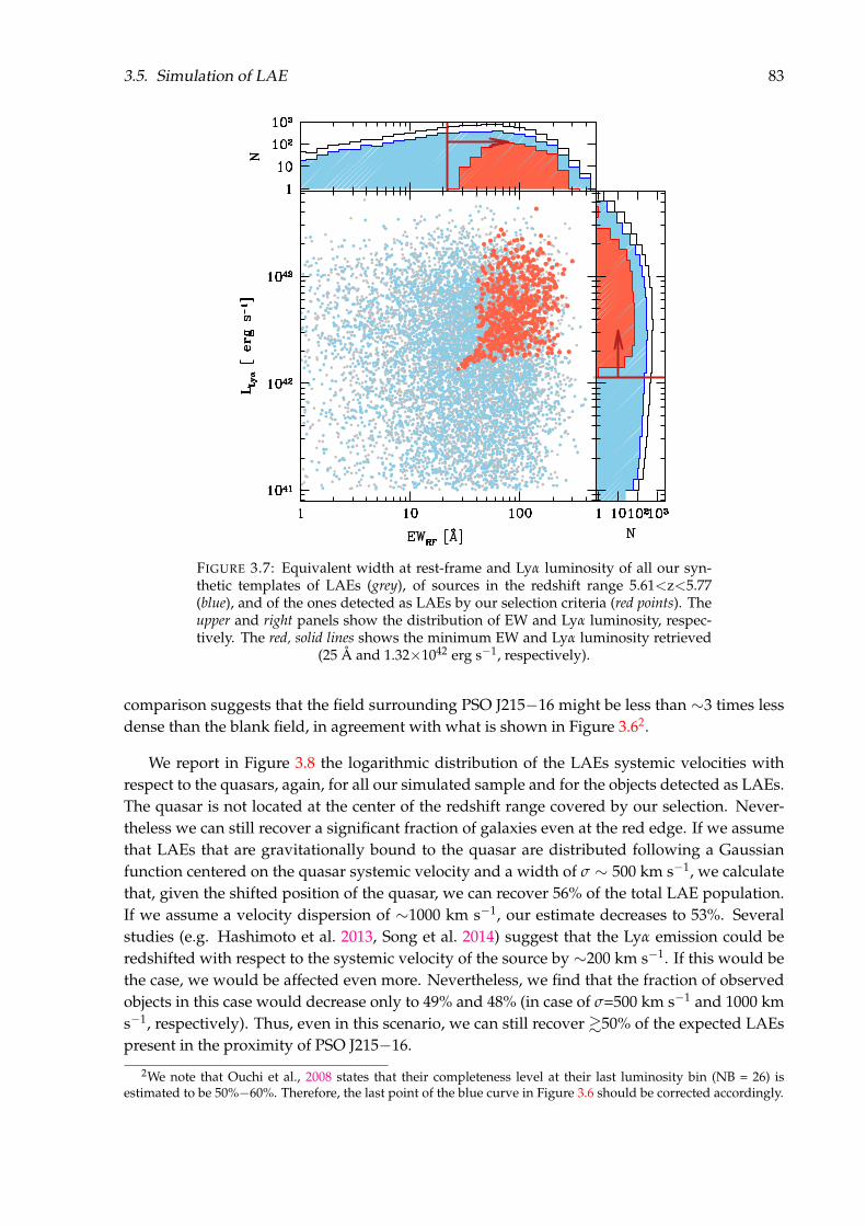
3.5. Simulation of LAE 83
FIGURE 3.7: Equivalent width at rest-frame and Lyα luminosity of all our syn-thetic templates of LAEs (grey), of sources in the redshift range 5.61<z<5.77(blue), and of the ones detected as LAEs by our selection criteria (red points). Theupper and right panels show the distribution of EW and Lyα luminosity, respec-tively. The red, solid lines shows the minimum EW and Lyα luminosity retrieved
(25 Å and 1.32×1042 erg s−1, respectively).
comparison suggests that the field surrounding PSO J215−16 might be less than ∼3 times lessdense than the blank field, in agreement with what is shown in Figure 3.62.
We report in Figure 3.8 the logarithmic distribution of the LAEs systemic velocities withrespect to the quasars, again, for all our simulated sample and for the objects detected as LAEs.The quasar is not located at the center of the redshift range covered by our selection. Never-theless we can still recover a significant fraction of galaxies even at the red edge. If we assumethat LAEs that are gravitationally bound to the quasar are distributed following a Gaussianfunction centered on the quasar systemic velocity and a width of σ ∼ 500 km s−1, we calculatethat, given the shifted position of the quasar, we can recover 56% of the total LAE population.If we assume a velocity dispersion of ∼1000 km s−1, our estimate decreases to 53%. Severalstudies (e.g. Hashimoto et al. 2013, Song et al. 2014) suggest that the Lyα emission could beredshifted with respect to the systemic velocity of the source by ∼200 km s−1. If this would bethe case, we would be affected even more. Nevertheless, we find that the fraction of observedobjects in this case would decrease only to 49% and 48% (in case of σ=500 km s−1 and 1000 kms−1, respectively). Thus, even in this scenario, we can still recover &50% of the expected LAEspresent in the proximity of PSO J215−16.
2We note that Ouchi et al., 2008 states that their completeness level at their last luminosity bin (NB = 26) isestimated to be 50%−60%. Therefore, the last point of the blue curve in Figure 3.6 should be corrected accordingly.

84 Chapter 3. The Environment of a z∼5.7 Quasar
FIGURE 3.8: Velocity distribution of mocked LAEs, with respect to the systemicvelocity of PSO J215−16 (short-dashed, blue line). In black we report the distributionof all the simulated sources, while in red only the sources recovered as LAEs. Thevelocity window encompassing +500 km s−1/-500 km s−1 with respect to thequasar is shown with long-dashed, green lines. The velocity window is not centeredon the redshift of the quasar, but we still recover &50% of the expected galaxies
population gravitationally bound to the quasar.
It is necessary to consider that our observed counts are also affected by Poisson noise andcosmic variance. Trenti and Stiavelli, 2008 provide estimates on the variance of the observednumber counts, taking into account both Poisson noise and cosmic variance, and based on avariety of parameters (e.g. the survey volume and completeness, the halo filling factor andexpected number of objects)3. In our case, we consider a cosmological volume V given byour field of view and a redshift interval of ∆z∼0.16, centered on z=5.69 (V∼14900 cMpc3, seeFigure 8); an intrinsic number of objects equals to the one recovered by our LAE simulation(23), a completeness of 67% (see Section 2 and Figure 3.3) and a Sheth-Tormen bias calculation.Kovac et al., 2007, studying the clustering properties of LAEs at z ∼4.5, find a value for theduty cycle of high redshift LAEs varying within 6%−50%. We consider here both extremecases. However, Kovac et al., 2007 consider a sample of LAEs with a minimum EW of 80 Å;since our EW limit is lower (25 Å, see Figure 3.7), we expect that the halo filling factor for ourcase would be closer to 50%. Then, we expect to observe 15± 7 (9) sources in the case of a dutycycle of 6% (50%), where the fractional uncertainty due to cosmic variance and Poisson noiseare 36% (49%) and 26% (in both cases), respectively. These results are consistent within 1.3σ, inthe first case, and 1σ in the second case with what expected in the present study.
Conversely, we can also obtain a rough estimate of the cosmic variance, for a populationof galaxies for which we know the expected number density in a certain volume, followingSomerville et al., 2004. They use cold dark matter models to derive the expected bias (b) and
3http://casa.colorado.edu/~trenti/CosmicVariance.html

3.6. Clustering 85
root variance of the dark matter (σDM) as a function of galaxy number density and survey vol-ume, respectively (see their Figure 3). We consider our survey volume as reported above, andan expected number density obtained integrating the LAE luminosity function until the Lyα
luminosity limit from our simulation (∼10−3 cMpc−3); we derive a fractional cosmic varianceof σv = bσDM ∼0.66 for a population of galaxies at z=6. This value is higher than what recov-ered using the method illustrated by Trenti and Stiavelli, 2008. Indeed, one needs to considerthat the cosmic variance is not a trivial quantity to estimate, and depend on several assump-tions considered in the models, e.g. the LAEs halo filling factor. Considering the latter valueobtained, we would expect to detect 23 ± 15 sources, which, taking into account our complete-ness, is consistent within 1σ with the observations reported here. Also, considering a clusteringscenario, e.g. consistent with the LAE-LAE clustering case (see Ouchi et al. 2003 and Section3.6), we would obtain 26 ± 18 sources, consistent with the observed ones.
3.6 Clustering
We may also study the environment of PSO J215-16 through a clustering approach. If quasarsand galaxies are indeed clustered, the excess of probability to find a galaxy at a distance r froma quasar, with respect to a random distribution of sources, can be estimated through the two-point correlation function (Davis and Peebles, 1983):
ξ(r) =(
rr0
)−γ
(3.6)
where r0 and γ are the correlation length and clustering strength, respectively. In order to ac-count for redshift distortions on the line of sight, we can consider instead the volume-averagedprojected correlation function. This is ξ(r) integrated over a line-of-sight distance d = 2vmax/aH(z)(with vmax maximum velocity from the quasar) and within a radial bin of width [Rmin, Rmax](Hennawi et al., 2006):
W(Rmin, Rmax) =
∫ d/2−d/2
∫ RmaxRmin
ξ(r)2πdRdr
V(3.7)
where V is the volume of the cylindrical shell:
V = π(R2max − R2
min)d (3.8)
Therefore, the number of galaxies that we expect to find around a quasar within a volume V inthe presence of clustering is:
NC = N(1 + W(Rmin, Rmax)) (3.9)
In case of no clustering, the number of sources expected is:
N = nV (3.10)
where n is the number density of galaxies per cMpc−3, above a certain limit in luminosity. Inthis scenario, N is equal to the number of galaxies found in a blank field within a cosmologicalvolume V.

86 Chapter 3. The Environment of a z∼5.7 Quasar
In this study, we calculate n by integrating the LAE luminosity function (Ouchi et al., 2008)down to the luminosity limit obtained by our simulation (1.32×1042erg s−1, see Section 3.5).We consider a line-of-sight distance given by vmax = 4000 km s−1 (consistent with the intervalprobed by our NB selection, see Sections 3.1 and 3.5, and Figure 3.8), Rmin = 0.001 cMpc andincreasing values of R = Rmax.
In Figure 3.9 we show the number of galaxies expected as function of R in case of no clus-tering (eq. 3.10), and in different scenarios of quasar-galaxy clustering (eq. 3.9). Since thereare currently no studies of LAE-quasar clustering at high redshift, we consider for comparisonsome other illustrative cases. We take values of r0 and γ obtained by observations of galaxy-quasar clustering at lower-z and LAE-LAE and quasar-quasar clustering at z ∼ 5.
FIGURE 3.9: Expected number of LAEs, given the depth reached in this study, asa function of projected distance from the quasar, in case of no clustering (e.g. arandom distribution of sources, yellow solid line), and for some illustrative clus-tering scenarios, taken from observational studies (Zhang et al. 2013, Ouchi et al.2003 and McGreer et al. 2016, short-dashed, long-dashed and dot-short-dashed line,respectively, see text for details). The counts of LAEs observed in this study arereported (not corrected for completeness). Also, we report the LAEs found byB13, and their expected number of sources in case of no clustering, taking intoaccount the depth of their study (dot-long-dashed line). For the sake of clarity, wedo not report the respective cases of clustering scenarios. We show the field ofview (F.O.V.) encompassed by our study. The errors are the poissonian noise onsmall counts from Gehrels, 1986. The counts of the observed LAEs are consistent
with what expected in a blank field.

3.7. Lyman Break Galaxies Analysis 87
Indeed, studies of galaxy-quasar clustering at z ∼1 (Zhang et al. 2013) estimate r0=6 h−1
cMpc and γ=2.14. Ouchi et al., 2003 derive the clustering properties of LAE at z = 4.86 from asample of objects detected in the Subaru Deep Field, for which they obtain r0 = 3.35 h−1 cMpcand γ=1.8. At high redshift, constraints on the quasar-quasar clustering properties are givenby the discovery of a close bright quasar pair, with only 21′′separation, at z∼5 (McGreer et al.,2016). The correlation function derived from this pair gives r0 >20 h−1 cMpc and γ=2.05. Weshow the number of LAEs found in this study. We also report the objects recovered by B13 andthe number of sources expected in their study in case of no clustering (since their observationsare shallower than the ones presented here, with a Lyα luminosity limit of 3.74×1042erg s−1,the number of background sources expected is lower).
Our number counts are consistent with a scenario of no clustering (i.e. the backgroundcounts, in line with what obtained in Section 3.4), and do not show evidence of strong clusteringin neither of the two quasar fields.
3.7 Lyman Break Galaxies Analysis
In addition to the LAE selection, we also search for LBGs using the dropout technique. SinceLBGs are expected to be characterized by a strong UV continuum, observed in the z filter, weuse the catalog obtained taking the z frame as our reference image. We consider all the sourceswith S/N>4 in z, and we apply only a selection using the broad band filters: we ask for a redR-z color (R-z>2) and, since we expect galaxies at these redshift to be faint, we require z>21.We recover 37 LBG candidates: we report the color-magnitude (R-z) vs z in Figure 3.10. It isworth to notice that, in the selection of LBG candidates, we are mainly limited by the depth ofthe R image (R2σ = 27.46) rather than by the z one; indeed, the faintest sources with (R2σ−z)>2would have z≤25.46 in our analysis (z5σ,lim = 25.96).
For comparison, we refer to the works by Brammer et al., 2012 and Skelton et al., 2014, whocompiled catalogs for some well-known extra-galactic fields, completed with spectroscopic andphotometric information. We consider four fields, that can be used as comparison blank fieldsfor our study: All-wavelength Extended Groth Strip International Survey (AEGIS), the CosmicEvolution Survey (COSMOS), the Great Observatories Origins Survey Northen field (GOODS-N) and the UKIRT InfraRed Deep Sky Survey (UKIDSS) Ultra Deep Field (UDS).
We selected LBG candidates from the catalogs imposing the same selection criteria as in thepresent study. In order to account for the different image depths, we consider only sourceswith z and R magnitude lower than the limits in our field (z< z5σ,lim = 25.96 and R< R2σ,lim =
27.46). The GOODS-N and UDS fields are shallower than our images in both R and z and onlyin the z frame, respectively. In these cases, we take as limits the corresponding values providedby Skelton et al., 2014 (z5σ,lim,GOODSN = 25.5, R2σ,lim,GOODSN = 27.19 and z5σ,lim,UDS = 25.9).We also consider the sample of LBG candidates recovered by B13 around ULAS J0203+0012
4We note, however, that the galaxies studied by Zhang et al., 2013 are not selected as LAEs but by consideringall the sources in the quasar field recovered in the SDSS-Stripe 82 catalog brighter (in the i-band) than a certainthreshold value, which depends on the field depth. This selection comprehends also passive and red galaxies.
5These values are in agreement with the ones found by Shen et al. (2007, r0=25.0 h−1 cMpc and γ=2), based ona sample of lower redshift (z > 3.5) bright SDSS quasars. However, we note that other quasar clustering studies,such as Eftekharzadeh et al., 2015, suggest much smaller clustering scales, with r0=7.59 h−1 cMpc (obtained from alower luminosity, z∼3.4, quasar sample; see also Section 3.8).

88 Chapter 3. The Environment of a z∼5.7 Quasar
FIGURE 3.10: Color-magnitude diagram (R-z) vs z. In grey points all the sourcesdetected in our field, considering the z frame as reference. The LBG candidatesfound from the z frame (37) are reported in blue squares. We show with verticaldashed lines the lower limit on the z magnitude (z > 21) and the 5σ upper limit(z=25.96). The horizontal line highlights our color criteria. The diagonal dashed linedisplays the 2σ limit magnitude in the R frame. The objects not detected in the Rframe at 2σ level are reported in blue triangles. The red diamond shows the quasar
position.
(20 sources), where they used an analogous selection method as the one described here. Theyreach limit magnitudes in the z and R bands of z5σ,lim,B13 = 25.14 and R2σ,lim,B13 = 27.29.
In Table 3.2 we report information on the comparison fields and on our field, i.e. coordi-nates, effective areas, literature references and characteristics of R and z filters. Although thedifferent fields were imaged with slightly different filter sets, the redshift windows covered arelarge (∆z ∼ 1.2) and corresponding to the one spanned in the present study6. We report thecumulative number counts, scaled to our effective area, of the sources found in the four blankfields and around the quasars (Figure 3.11). The difference between the counts obtained in theUDS field with respect to the counts in the other blank fields may be due to a diverse contri-bution of contaminant sources. Indeed, the UDS field was imaged through a R filter slightlyredder than the ones used in the other fields (see Table 3.2): this might turn into a more conser-vative selection of high-redshift LBGs. Recent studies suggest also that the UDS field might beintrinsically underdense in z∼6 galaxies with respect to other well-known fields (Bowler et al.2015, Bouwens et al. 2015b).
6With the filters used, in the AEGIS and COSMOS fields we span 5.2 . z . 6.3, ∆z ∼ 1.1, in the GOODS-N field5.2 . z . 6.4, ∆z ∼ 1.2, while in the UDS field 5.4 . z . 6.5, ∆z ∼ 1.1. In the present study and in B13 we areselecting sources in 5.2 . z . 6.5, ∆z ∼ 1.3.

3.7.Lym
anBreak
Galaxies
Analysis
89
TABLE 3.2: Field names, coordinates, effective areas and technical characteristics for the R and z filters of our comparison fields and theone studied here. The areas analyzed in this study and in B13 differ due to the diverse masking. References from the literature are: (1)
Hildebrandt et al., 2009, (2) Erben et al., 2009, (3) Capak et al., 2004, (4) Furusawa et al., 2008, (5) Bañados et al., 2013, (6) This work.
Field RA DEC Effective Area λc,R ∆λR λc,z ∆λz Instrument Reference[J2000.0] [J2000.0] [arcmin2] [Å] [Å] [Å] [Å]
AEGIS 14:18:36.00 +52:39:0.00 88 6245 1232 8872 1719 MegaCam@CFHT (1), (2)COSMOS 10:00:31.00 +02:24:0.00 154 6245 1232 8872 1719 MegaCam@CFHT (1), (2)
GOODS-N 12:35:54.98 +62:11:51.3 93 6276 1379 9028 1411 Suprime-Cam@Subaru (3)UDS 02:17:49.00 −05:12:2.00 192 6508 1194 9060 1402 Suprime-Cam@Subaru (4)B13 02:03:32.38 00:12:29.06 44 6550 1650 9100 1305 FORS2@VLT (5)
This work 14:20:36.39 -16:02:29.94 37 6550 1650 9100 1305 FORS2@VLT (6)

90 Chapter 3. The Environment of a z∼5.7 Quasar
We can compare the cumulative number counts of LBGs in the field of the quasar studiedhere with the ones found in the comparison blank fields. In order to avoid incompleteness is-sues in the low-luminosity end, we take only sources with R<Rlim,5σ, considering the GOODSNfield, which is the shallowest among our fields (Rlim,5σ=26.2). Taking into account our color se-lection criterion, we obtain a resulting z magnitude limit of 24.2. At this limit, the counts ofthe LBG candidates in our quasar field is consistent within 1σ with the counts in the UDS field,and lower than the ones in AEGIS, COSMOS and GOODS-N fields by ∼1.7, 1.3 and 1.1σ re-spectively. The quasar field analyzed here appears only marginally (∼1.1σ) denser than theone studied in B13. These results are hence in agreement with B13, where no overdensity ofLBGs with respect to a blank field was found.
Some general caveats are to be taken into account. Considering our broad selection criteria,both our sample and the ones derived from the comparison fields might be contaminated byred, lower redshift sources. We employ the further information provided in the catalogs of thecomparison fields in order to better characterize the sources retrieved by our LBGs selection.We can consider the available photometric redshift estimates, computed with the public codeEAZY (Brammer, van Dokkum, and Coppi 2008), which take into account all the photometricinformation present in the catalog. We take only the objects with a reliable redshift estimate,as based on the quality parameter Qz (Qz < 2.0, see Brammer, van Dokkum, and Coppi 2008),and for which zphot ≥5.0. Only the 6%, 10%, 4% and 9% of the LBG sample from, respectively,AEGIS, COSMOS, GOODS-N and UDS field could be identified as high-redshift galaxies (seeTable 3.3), while the vast majority was better fitted by a z∼1 galaxy model. This simple testshows how the selection criteria used here, without the help of further bands, lead us to ahighly contaminated sample.
In summary the LBGs selection also does not reveal a possible overdensity around thequasar. However, due to the wide redshift range considered, an enhancement in the num-ber of LBGs in the quasar field would represent an indication, more than solid evidence, for thepresence of an overdensity of galaxies in the proximity of the quasar.
TABLE 3.3: Field names, total number of LBG candidates retrieved by our pho-tometric cuts and number of sources with photometric redshift estimates corre-
sponding to zphot ≥ 5.
Field Number LBGs Number phot LBGs
AEGIS 176 11COSMOS 257 26GOODS-N 186 7UDS 187 17
3.8 Discussion
We do not find evidence for an overdensity of LAEs in an area of ∼37 arcmin2 centered on thez ∼5.73 quasar PSO J215−16. Here we investigate possible scenarios to explain our findings.
• The overdensity is more extended than our field of view
Overzier et al., 2009 and, more recently, Muldrew, Hatch, and Cooke, 2015, through a

3.8. Discussion 91
FIGURE 3.11: Cumulative Number Counts of LBGs at z∼6. All the counts arescaled for the effective area in our study. We report the candidates found aroundthe z=5.73 quasar PSO J215−16 (red squares) and the quasar ULAS J0203+0012(orange triangles, B13), slightly shifted with respect to the other fields in order toavoid confusion. We show the sources selected, using the same selection criteriaand image depth, in four comparison blank fields (AEGIS-cyan, COSMOS-brown,GOODS-N-blue and UDS-green circles). The result obtained considering all theblank fields together is shown with black circles. The errors are taken from the
poisson noise in case of low counts statistics (Gehrels 1986).
combination of N-body simulations and semi-analytical models, find that overdensitiesof galaxies at z∼6 are expected to be very extended, and can cover regions up to ∼25−30arcmin radius, corresponding to &20 pMpc at that redshift. In the present study we coveronly a region of ∼1 pMpc transversal radius, and we might be missing a large part of apotential overdensity7.From an observational perspective, enhancements in the number of galaxies around quasarshave been reported on rather modest scales, comparable to ours or even smaller. How-ever, there are indications, based on LBGs searches, that some quasars are surrounded byoverdensities on larger scales, even if a further spectroscopic confirmation is needed (seeSection 1.5.4).In Table 3.4 we show a summary of the findings obtained by diverse studies, where theyconsidered different areas and techniques (see also Section 1.5.4).In our case, in order to discard or confirm this scenario, we would need further observa-tions covering a wider area (e.g with a radius of &20 arcmin).
7We would like to stress that, in the hypothesis that the quasar occupies the center of a z ∼6 overdensity similarto the one found by Toshikawa et al., 2014 in a blank field, searches in area of∼2−3 pMpc should still show evidenceof an enhancement in the number of galaxies with respect to a blank field.

92 Chapter 3. The Environment of a z∼5.7 Quasar
TABLE 3.4: List of z>5 quasars whose large-scale fields were inspected for thepresence of galaxy overdensities. We report the quasars names, redshifts, litera-ture references, instruments used and area covered in each study (in comovingand physical Mpc2 at z ∼6). The references are coded as: (1) Stiavelli et al., 2005,(2) Willott et al., 2005, (3) Zheng et al., 2006, (4) Kim et al., 2009, (5) Utsumi et al.,2010, (6) Husband et al., 2013, (7) Bañados et al., 2013, (8) Simpson et al., 2014, (9)Morselli et al., 2014, (10) McGreer et al., 2014 , (11) this work. All these studies,except for Bañados et al., 2013 and this work which searched for LAEs, are basedon i-dropout selection. We report also whether the fields were found overdense(+), underdense (-) or consistent (0) with respect to a comparison blank field. Wenote cases in which the same field was found consistent with a blank field wheninspected on small scales, while overdense when studied over larger scales (e.g.SDSS J1048+4637 and SDSS J1148+0356). The overdensity reported by Utsumiet al., 2010, even if found with the Subaru SuprimeCam, spreads across an areaof ∼ 3Mpc radius, therefore it would have been detected also by searches over
smaller fields of view.
Object Redshift Ref Instrument FoV FoV Overdensity[cMpc2] [pMpc2]
ULAS J0203+0012 5.72 (7) VLT FORS2 250 5.6 0SDSS J0338+0021 5.03 (6) VLT FORS2 250 5.6 +SDSS J0836+0054 5.82 (3) HST ACS 65 1.4 +SDSS J1030+0524 6.28 (1) HST ACS 65 1.4 +
(2) GMOS-N 170 3.7 0(4) HST ACS 65 1.4 +(9) LBT LBC 3136 64.0 +
SDSS J1048+4637 6.20 (2) GMOS-N 170 3.7 0(4) HST ACS 65 1.4 0(9) LBT LBC 3136 64.0 +
ULAS J1120+0641 7.08 (8) HST ACS 65 1.4 0SDSS J1148+0356 6.41 (2) GMOS-N 170 3.7 0
(4) HST ACS 65 1.4 -(9) LBT LBC 3136 64.0 +
SDSS J1204−0021 5.03 (6) VLT FORS2 250 5.6 +SDSS J1306+0356 5.99 (4) HST ACS 65 1.4 -SDSS J1411+1217 5.95 (9) LBT LBC 3136 64.0 +SDSS J1630+4012 6.05 (4) HST ACS 65 1.4 +
CFHQS J2329−0301 6.43 (5) Subaru SuprimeCam 4600 83.3 +CFHQS J0050+3445 6.25 (10) HST ACS & WFC3 29 0.6 -
PSO J215.1512−16.0417 5.73 (11) VLT FORS2 206 4.5 0
• The ionizing emission from the quasar is preventing structure formation in its immediate proxim-ities
Strong radiation from a bright quasar can ionize its nearby regions (up to ∼1−5 pMpcradius around z ∼6 quasars, e.g. Venemans et al. 2015b, Eilers et al. 2017, and Section2.5.10, Figure 2.19), with an increase in both the temperature and ionized fraction of theIGM, and in the intensity of the local UV radiation field.The effects on the visibility of the Lyα radiation in this region are not straightforward todeduce. As a consequence of the increase in the UV background radiation field, a higherLyα transmission flux value is expected around the quasar with respect to the typicalIGM environment at the same redshift (Bruns et al. 2012). However, in addition to therise in the UV background, also the nearby IGM temperature increases. Thus, the isother-mal virial temperature necessary for gas accretion in the dark matter halo is higher, andthe mass needed to form a structure increases (Jeans-mass filtering effect, Gnedin 2000).Even if the Lyα transmission flux is supposed to be higher, the formation of galaxies itselfis suppressed, especially for objects in the low-mass end (e.g. Shapiro, Iliev, and Raga

3.8. Discussion 93
2004). Utsumi et al., 2010 invoke this effect in order to explain the absence of galaxies ina region of ∼3 pMpc radius around a z∼6 quasar (see Section 1 and Table 3.4). Given thetypical sizes of quasar’s ionized regions, and that in our study we cover scales of only∼2 pMpc, suppression of galaxy formation due to the quasar ionizing radiation mightexplain the lack of LAEs.
• The bulk of the overdensity population is composed by dusty/obscured galaxies.
Observations find that host galaxies of z >5 quasars contain a considerable amount ofdust (∼108−109 M) and molecular gas (∼1010 M, e.g. Decarli et al. 2018; see Sections1.5 and 2.5.9). They are already characterized by a metal-enriched medium, comparableto what is observed at low redshift (e.g. De Rosa et al. 2011; see Section 2.5.8). One mightforesee that also the galaxies assembling in the proximity of the quasar might be charac-terized by a high dust/molecular gas content.Indeed, on the theoretical side, Yajima et al., 2015, implementing a 3D radiation trans-fer code in a high resolution cosmological simulation, show that overdense regions atz ∼ 6, where quasars are supposedly found, host more evolved, disk-like and massive(M∗ ∼1011 M) galaxies, with respect to an average field at the same redshift. Theyare characterized by a strong dust extinction (i.e. a low UV radiation escape fraction,fesc .0.1), and a powerful star formation (SFR &100 M yr−1); therefore they are verybright in the IR, with LIR as high as ∼ 4×10¹² L. These massive and highly obscuredobjects, whose detection in the UV rest-frame might be hindered by absorption and/orstrongly dependent on orientation effects, rather than LAEs (i.e. young, dust-poor starforming galaxies), may be a more suited tracer for high redshift, massive overdensities(see Section 1.5.4 and Chapter 4).Further studies of the environment of high redshift quasars with sub-mm facilities (inparticular ALMA) are starting to test this scenario, allowing us to recover a possible pop-ulation of dusty galaxies in the quasar field. However, we note that, due to the smallfield of view of ALMA (with a size of ∼ 20′′, corresponding to ∼ 800 ckpc ∼ 110 pkpcat z ∼ 6), we would be able to search only the most proximate region around the quasar.A study of the fields around three z>6.6 quasars with ALMA did not find an excess ofdusty galaxies in a region of 65 ckpc radius (Venemans et al. 2016); however, several re-cent studies spot instead such overdensities of mm–bright galaxies (see Section 1.5.4 andChapter 4).
• Quasars at high redshift do not inhabit massive dark matter halos
The quasar two-point correlation function at low redshift (z .2.5), as derived from boththe 2dF QSO Redshift Survey (Croom et al. 2005) and the SDSS (Ross et al. 2009) quasarsample, shows that quasars are commonly associated with average-mass dark matterhalos (i.e. MDMH ∼ (2-3)×1012 M), far less massive than the most massive halos at thesame redshift (∼1014 − 1015 M), independently of the quasar luminosity.At higher-z (3.5. z .5.4) the scenario is less clear: based on the SDSS sample, Shen et al.,2007 calculate an average dark matter host halo mass of (4-6)×1012 M, slightly higherthan the results at lower redshifts. However, more recent studies, based on the final SDSSIII-BOSS quasar sample, do not find a clear evolution of quasar clustering from z ∼ 0 toz ∼ 3 (Eftekharzadeh et al. 2015)8.
8We note that the quasars considered here are less massive than the ones studied by Shen et al., 2007

94 Chapter 3. The Environment of a z∼5.7 Quasar
From a theoretical point of view, there have been studies suggesting that quasars alsoat high redshift (z&5) inhabit dark matter halos with average masses (i.e. less massivethan the most massive halos at that epoch). In particular, Fanidakis et al., 2013 performsimulations based on the semi-analytical model GALFORM, in order to study the relationbetween quasars and dark matter halos up to z ∼6. They show that, in case of models inwhich AGN feedback is considered, the masses of the dark matter host halos are roughly∼ 1012 M, from z ∼0 to z ∼6: this is an order of magnitude lower than the most massivehalos at z ∼6 obtained in the same simulation, and is in agreement with observations atlow redshift. However, as argued by Simpson et al., 2014, it is worth to notice that thesimulations by Fanidakis et al., 2012 fail to create the most massive black holes (M&109
M) at z ∼6, while they appear only at z ∼4. Therefore, the claims reported here are tobe taken with caution, and may not hold in every scenario.
In summary, in this Chapter we studied the environment of the z ∼5.73 quasar PSO J215−16searching for LAEs using broad and narrow-band VLT imaging, on Mpc-scales, i.e. ∼2 pMpc∼14 cMpc at the redshift of the quasar. This is the second study in which we do not findevidence of an overdensity of Lyα emitting sources in a quasar field, compared to blank fields(see also B13).
Studies on wider areas (>20 arcmin radius, corresponding to ∼8 pMpc ∼ 47 cMpc at theredshift of the quasar), with the support of further, multiwavelength observations (i.e. IR/sub-mm), are required in order to discriminate among these scenarios. However, it is intriguingto note that overdensities of galaxies around radio-loud sources (both radio-loud galaxies andAGN) have been extensively reported (e.g. Venemans et al. 2007, Wylezalek et al. 2013). Inthe future, it appears to be worthwhile to repeat our experiment on z > 6 radio-loud quasars,whose sample has been substantially increased recently (Bañados et al. 2015a), to potentiallytarget the earliest galactic structures (see also Section 5.1.2 for further discussion on this point).

95
Chapter 4
Highly Obscured Companion Galaxiesaround z ∼6 Quasars
In this chapter, we present new sensitive optical/NIR follow-up observations specifically de-signed to probe four companion galaxies to 6 . z . 6.6 quasars and obtained from severalground- and space-based facilities. In particular, we aim to observe the bulk of their stellaremission in the rest-frame optical wavelength range, in order to assess their total stellar mass(M∗). We also aim to uncover their rest–frame UV radiation, to probe the contribution from theyoung stellar population and the budget of the unobscured star formation.
In § 4.1, we describe our sample and report our observations and data reduction. In § 4.2.1,we compare our measured photometry with spectral energy distributions of illustrative casesof local galaxies, and we use a SED fitting code for one source. The relative obscured andunobscured contribution to the star formation rate are examined in § 4.2.2, while in § 4.2.3 weplace our findings in the context of observations of star forming galaxies and SMGs at z &6.Finally, we discuss the case of a source detected solely in the dust continuum emission in § 4.3,and we present our conclusions in § 4.4.
4.1 Observations and Data Reduction
Our sample is composed by three (out of the four) quasar+companion systems presented inDecarli et al., 2017: SDSS J0842+1218, PSO J231.6576–20.8335 and CFHQS J2100−1715 (here-after J0842, PJ231 and J2100, respectively; see Section 1.5.4). We also consider the quasarPSO J167.6415–13.4960 (hereafter PJ167), whose companion galaxy was recently observed withALMA by Willott, Bergeron, and Omont (2017; see Section 1.5.4). In the following sections,we will refer to all the respective companions as “quasar_short_name”c. The coordinates,redshifts, spatial and velocity separations of the quasars and respective companion galaxies,obtained from ALMA observations, are reported in Table 4.1.
We also obtained data for a bright source, detected only in the dust continuum emission,close to the quasar VIK J2211−3206 (hereafter J2211; Venemans et al. in prep)1. This galaxy ispart of the sample of dust continuum emitting sources discovered around several z ∼6 quasarsthat will be discussed by Champagne et al. (in prep), for which no secure redshift confirma-tion is however available. We present our follow–up data and discuss our constraints on theproperties of this source in Section 4.3.
1This quasar was also recently independently discovered by Chehade et al., 2018, with the name of VST-ATLASJ332.8017-32.1036.

96 Chapter 4. Highly Obscured Companion Galaxies around z ∼6 Quasars
We collect the available observations of the fields in our sample, either from the literature orobtained with dedicated follow-up campaigns. Details on the observations used here, i.e. dates,instruments/telescopes, exposure times and filters, are shown in Table 4.2.
4.1.1 Optical/NIR Spectroscopy
We observe the companions of PJ231 and J0842, and the quasar PJ231, with the Magellan/FIREspectrograph (Simcoe et al., 2008) at the Magellan Telescope. The data are reduced followingstandard techniques, including bias subtraction, flat field and sky subtraction. The wavelengthcalibration is obtained using sky emission lines as reference (see also Bañados et al. 2014). Weuse the standard stars HIP43018 and HIP70419 to flux calibrate and correct for telluric contam-ination in the spectra of J0842c and PJ231/PJ231c, respectively. In order to obtain the absoluteflux calibration, we scale the spectrum of PJ231 to match the respective observed J band magni-tude (J =19.66±0.05; see Table 2.3 in Section 2.3.2). We use the same factor to scale the spectraof the companions. No clear emission from either of the two companion is detected in the ob-served spectra (see Figure 4.1). We estimate the 3σ limits on the Lyα broad emission line byconsidering the 3×mean value of the spectral error vector in a window of 200 Å around theexpected location of the emission line, based on the redshift derived from the ALMA [CII] ob-servations. These limits are of 1.4 and 1.0×10⁻¹⁷ [erg s−1 cm−2 Å] for J0842c and PJ231c, re-spectively.
−1
0
1
2
3 PJ231 COMPz[CII]= 6.59± 0.0008
9000 10000 11000 12000−1
0
1
2
3 J0842 COMPz[CII]= 6.0656± 0.0007
Wavelength [A]
Flu
xD
ensi
ty[1
0−17
erg
s−1
cm−2
A−1
]
FIGURE 4.1: Spectra of the companions of the quasars PJ231 (top) and J0842 (bot-tom panel), acquired with the FIRE spectrograph. The dashed blue lines highlightthe expected positions of the respective Lyα emission lines, established from theobservations of the narrow [CII] emission line with ALMA. The surrounding re-gions of ±100 Å, used to estimate limits on the Lyα emission line in the compan-
ion galaxies, are also shown with light blue shaded areas.

4.1.O
bservationsand
Data
Reduction
97
TABLE 4.1: Coordinates, redshifts, spatial projected distances and velocity shifts of the quasars and the adjacent galaxies studied in thiswork. These measurements are obtained from the narrow [CII] emission line and underlying dust continuum observed by ALMA. Theanalogous quantities for the companion of J2211, detected solely in the dust continuum emission (see Section 4.3) are shown is Table
4.5. References are: (1) Decarli et al., 2017, (2) Decarli et al., 2018 and (3) Willott, Bergeron, and Omont, 2017.
Name R.A. (J2000) Decl. (J2000) z zerr ∆rprojected ∆vline of sight References[kpc] [km s−1]
SDSS J0842+1218 08:42:29.43 12:18:50.4 6.0760 0.0006 (1)SDSS J0842+1218c 08:42:28.95 12:18:55.1 6.0656 0.0007 47.7 ± 0.8 -443 (1)PSO J167.6415–13.4960 11:10:33.98 -13:29:45.6 6.5148 0.0005 (2)PSO J167.6415–13.4960c 11:10:34.03 -13:29:46.3 6.5090 – 5.0 -270 (3)PSO J231.6576–20.8335 15:26:37.84 -20:50:00.8 6.58651 0.00017 (1)PSO J231.6576–20.8335c 15:26:37.87 -20:50:02.3 6.5900 0.0008 8.4 ± 0.6 +137 (1)CFHQS J2100−1715 21:00:54.70 -17:15:21.9 6.0806 0.0011 (1)CFHQS J2100−1715c 21:00:55.45 -17:15:21.7 6.0796 0.0008 60.7 ± 0.7 -41 (1)

98C
hapter4.
Highly
Obscured
Com
panionG
alaxiesaround
z∼
6Q
uasars
TABLE 4.2: Information on the optical/IR spectroscopy and imaging data used in this work. Together with the newly acquired obser-vations presented here, we consider archival data for the quasar J0842, obtained with Spitzer/IRAC in the [5.8] and [8.0] channels, andwith HST/WFC3 in the F105W filter (Leipski et al. 2014; see Section 4.1). We will focus on the dust–continuum detected source close to
the quasar VIK J2211−3206 in Section 4.3.
Name Date/Program ID Telescope/Instrument Filters/λ range Exp. Time
SDSS J0842+1218 2016–03–15 Magellan/FIRE 0.82–2.49 µm 4176s2017–04–27 / 14876 HST/WFC3 F140W 2612s2011–01–22 / 12184 HST/WFC3 F105W 356s2017–02–09 / 13066 Spitzer/IRAC 3.6, 4.5 µm 7200s2007–11–24 / 40356 Spitzer/IRAC 5.8, 8 µm 1000s
PSO J167.6415–13.4960 2017–08–11 / 14876 HST/WFC3 F140W 2612s2017–04–13 / 13066 Spitzer/IRAC 3.6, 4.5 µm 7200s
PSO J231.6576–20.8335 2016–03–15 Magellan/FIRE 0.82–2.49 µm 4788s2017–04–01 / 14876 HST/WFC3 F140W 2612s2016–11–25 / 13066 Spitzer/IRAC 3.6, 4.5 µm 7200s
CFHQS J2100−1715 2016–09–18/19 / 334041 LBT/LUCI J 10440s2017–05–04 / 14876 HST/WFC3 F140W 2612s2017–01–14 / 13066 Spitzer/IRAC 3.6, 4.5 µm 7200s
VIK J2211−3206 2017–04–28 / 14876 HST/WFC3 F140W 2612s2017–01–29 / 13066 Spitzer/IRAC 3.6,4.5 µm 7200s

4.1. Observations and Data Reduction 99
4.1.2 IR Photometry
We list here the observations and data reduction of the imaging follow–up data, obtained withground– and space–based instruments.
LUCI @ LBT
We image the field of J2100 in the J band with the LBT Utility Camera in the Infrared (LUCI1and LUCI2; Seifert et al. 2003) at the LBT, in binocular mode. We reduce the data follow-ing standard techniques, i.e. we subtract the master dark, divide for the master flat field, andmedian–combine the frames after subtracting the contribution from the background and afteraligning them using field stars. We find the final astrometric solution using as reference theGAIA Data Release 1 catalog2 (DR1; Gaia Collaboration et al. 2016b, 2016). We flux-calibratethe image with respect to the 2MASS Point Source Catalog. The seeing of the reduced imageis 0.′′98. We calculate the depth of the image by distributing circular regions with radius equalto half of the seeing over the frame, in areas with no sources. We consider as the 1σ error ofour image the σ of the gaussian distribution of the fluxes calculated in these apertures. We donot detect, at S/N>3, any emission at the location of the companion, after performing forcephotometry on an area corresponding to the seeing (see Figure 4.2). The 3σ limit magnitude,that we will consider in the following analysis, is equal to J=26.24.
WFC3 @ HST
We obtain new observations of all the targets studied here with the Wide Field Camera 3(WFC3), on board HST, using the F140W filter (λc =1.3923 µm and ∆λ =0.384 µm; ProgramID:14876, PI: E. Bañados). For the quasar J0842, previous WFC3 observations in the F105W fil-ter (λc =1.0552 µm and ∆λ =0.265 µm) were also retrieved from the Hubble Legacy Archive3
(Program ID:12184,PI: X. Fan). We refer to Table 4.2 for further details on this dataset.
We analyze both the archival and new observations in a consistent way. We consider thereduced data produced by the HST pipeline, and we take the zero-point photometry from theWFC3 Handbook4. We re-calibrate the images astrometry using the GAIA DR1 catalog. Wecalculate the depth of the images in an analogous way as performed above for our LUCI data,considering here areas of 0.4′′radius (containing the 84% of the flux of a point source5). Weperform aperture photometry, using this aperture radius, at the positions of the companions.The companion sources of J0842, J2100 and PJ231 are not detected in the F140W filter, andJ0842c is not detected in the F105W image. We report all the 3σ limit fluxes in Table 4.3. Weshow the observations of all the fields studied in this work in the F140W filter in Figure 4.3,and the F105W image of J0842 in Figure 4.4.
In the case of PJ167, the companion is located at a projected distance of only 0.9′′, and itis blended with the quasar emission. In order to recover meaningful constraints on the pho-tometry of PJ167c, it is necessary to subtract the quasar contribution, by modeling the imagePSF. We use the bright star 2MASS J11103221–1330007, in the proximity of PJ167, in order to
2https://www.cosmos.esa.int/web/gaia/dr13https://hla.stsci.edu/4http://www.stsci.edu/hst/wfc3/analysis/ir_phot_zpt5http://www.stsci.edu/hst/wfc3/analysis/ir_ee

100 Chapter 4. Highly Obscured Companion Galaxies around z ∼6 Quasars
create an empirical PSF model from the same image. This source is located at a distance of only30′′ from the quasar, limiting the errors due to the changes in the shape of the PSF over thefield. Its J and H magnitudes, from the 2MASS Point Source Catalog, are 15.249 and 15.105,respectively. The corresponding J − H color of 0.144 is therefore close to that of the quasar(J − H=0.216). We shift, scale and subtract the PSF model from the quasar emission using thesoftware GALFIT (version 3.0.5; Peng et al. 2002, 2010). In Figure 4.5 we show the native HSTimage, the PSF star model and the residual frame, in which the bright quasar emission has beensubtracted. The companion galaxy is well isolated, and its F140W PSF magnitude, measuredwith GALFIT, is equal to 25.48 ± 0.17. Diffuse emission, extending from the companion to thequasar, is also tentatively recovered. Additional, high resolution imaging and spectroscopy isneeded to securely confirm and characterize such emission.
Summarizing, in the following analysis we adopt the F140W 3σ limit magnitudes for J2100c,PJ231c and J0842c. For this last object, we also measure the 3σ limit magnitude in the F105Wband from archival data. We consider the F140W PSF magnitude for PJ167c. All these quanti-ties, converted into fluxes, are reported in Table 4.3.
315°13'36"42"48"54"14'00"RA (J2000)
36.0"
30.0"
24.0"
18.0"
-17°15'12.0"
Dec
(J200
0) Q
C
20 pkpc20
0
20
40
60
80
FIGURE 4.2: Postage stamp (30′′×30′′) of the field around the quasar J2100, im-aged in the J filter with the LUCI1 and LUCI2 cameras at the LBT (see Section 4.1.2and Table 4.2). No emission at the location of the companion galaxy (marked with
a red circle of 1′′radius) is recovered at S/N> 3.
IRAC @ Spitzer
The fields of all the objects in our sample were recently observed in the [3.6] (λc =3.550 µm and∆λ =0.750 µm) and [4.5] (λc =4.493 µm and ∆λ =1.015 µm) filters with the InfraRed ArrayCamera (IRAC; Fazio et al. 2004; Program ID:13066, PI: C. Mazzucchelli; see Table 4.2). We

4.1. Observations and Data Reduction 101
also use archival data of J0842 (Program ID:40356, PI: X. Fan), covering the IRAC filters [5.8](λc =5.731 µm and ∆λ =1.425 µm) and [8.0] (λc =7.872 µm and ∆λ =2.905 µm; see Table 4.2).
We adopt the reduced data from the Spitzer pipeline, and the photometric calibration (i.e. pho-tometric zero point and aperture correction values) specified in the IRAC Instrument Note-book6. We refine the astrometric solution re-calibrating the pipeline-reduced images using theGAIA DR1 catalog. Given the limited spatial resolution of the IRAC camera (0.6 arcsec/pixel)and the depth of our [3.6] and [4.5] images, the companion galaxies studied here are blendedeither with the emission of the much brighter quasar, or with that of foreground sources (seeFigure 4.3). Hence, one needs to properly model and remove these emissions.
In order to model the PSF function, which is undersampled in the IRAC data, we re-samplethe native images over a grid of 0.12 arcsec/pixel resolution, using the IRAF task magnify.In each magnified image, we select a collection of stars in a 1′×1′ window centered on thequasar, in order to minimize the effect of the changes to the PSF shape due to the location onthe detector; we use the corresponding HST/WFC3 images as reference to pick isolated stars.We obtain the final PSF model for each image by shifting, aligning, scaling and combining theselected stars. The number of stars used ranges between 4 and 9, in case of the [4.5] image of thequasar J2100, and of the [3.6] image of the quasar PJ231, respectively. We use GALFIT in order tosample the PSF image to the original resolution, and to model and subtract the emission fromthe quasar and eventual foreground objects.
In Figure 4.3, we show the postage stamps of the IRAC [3.6] and [4.5] images, and the cor-responding images of the residuals. No clear emission from the companion galaxies is detectedin the residual images. We quantify the limits on the photometry of the companions as follows.For each image, we run GALFIT subtracting at the exact position of the companion a sourcemodeled with a PSF function and scaled to a fixed magnitude, which we vary between 21 and25, in steps of 0.01 mag. When adopting magnitudes smaller (i.e. brighter fluxes) than the limitmagnitude to which our image is sensitive, the subtraction will leave a negative residual. Inthe residual image, we perform aperture photometry at the companion position in an apertureof 2.4′′ radius, and we compare the measured flux with the image 3σ flux limit. This flux limitis measured on the same area used for the force photometry, and by evaluating the backgroundrms in an annulus of radius 14′′ and width of 10′′ centered on the companion. We assume thatthe 3σ limit magnitude is the value at which the measured absolute flux in the residual imageis equal to the 3σ flux limit. We report these values in Table 4.3.
Finally, we analyze the archival J0842 Spitzer/IRAC observations (see Figure 4.4): these ob-servations are much shallower (see Table 4.2), since they were devised to only detect the brightquasar. No foreground objects overlaps the companion location, and we therefore performaperture photometry on the native images, using the same aperture as in the observations inthe [3.6] and [4.5] channels. We measure no detection at S/N>3, and we consider the corre-sponding 3σ limit fluxes.
To summarize, in Table 4.3 we report the photometric measurements (or limits) for com-panion galaxies of z ∼6 quasars obtained from the observations described above. We also listtheir fluxes at λobs =1.2 mm from ALMA observations (Decarli et al., 2017).
6http://irsa.ipac.caltech.edu/data/SPITZER/docs/ irac/iracinstrumenthandbook/IRAC_Instrument_Handbook.pdf

102C
hapter4.
Highly
Obscured
Com
panionG
alaxiesaround
z∼
6Q
uasars
167°38'20"24"28"32"36"40"
52.0"
48.0"
44.0"
40.0"
-13°29'36.0"
QC
20 pkpc0.10
0.05
0.00
0.05
0.10
0.15
167°38'20"24"28"32"36"40"
QC
20 pkpc 0.03
0.04
0.05
0.06
0.07
167°38'20"24"28"32"36"40"
C
20 pkpc0.00
0.01
0.02
0.03
167°38'20"24"28"32"36"40"
QC
20 pkpc0.110
0.115
0.120
0.125
0.130
0.135
0.140
0.145
167°38'20"24"28"32"36"40"
C
20 pkpc 0.010
0.005
0.000
0.005
0.010
0.015
0.020
0.025
0.030
130°37'12"16"20"24"28"
+12°18'44.0"
48.0"
52.0"
56.0"
19'00.0"
QC
20 pkpc0.05
0.00
0.05
0.10
0.15
130°37'12"16"20"24"28"
QC
20 pkpc 0.11
0.12
0.13
0.14
0.15
130°37'12"16"20"24"28"
C
20 pkpc 0.010
0.005
0.000
0.005
0.010
0.015
0.020
130°37'12"16"20"24"28"
QC
20 pkpc0.37
0.38
0.39
0.40
0.41
130°37'12"16"20"24"28"
C
20 pkpc0.02
0.01
0.00
0.01
0.02
0.03
231°39'20"24"28"32"36"
08.0"
04.0"
50'00.0"
56.0"
-20°49'52.0"
Q
C
20 pkpc 0.10
0.05
0.00
0.05
0.10
231°39'20"24"28"32"36"
Q
C
20 pkpc0.130
0.135
0.140
0.145
0.150
231°39'20"24"28"32"36"
C
20 pkpc 0.015
0.010
0.005
0.000
0.005
0.010
0.015
231°39'20"24"28"32"36"
Q
C
20 pkpc 0.370
0.375
0.380
0.385
0.390
0.395
0.400
231°39'20"24"28"32"36"
C
20 pkpc 0.020
0.015
0.010
0.005
0.000
0.005
0.010
0.015
0.020
315°13'36"40"44"48"52"56"
28.0"
24.0"
20.0"
16.0"
-17°15'12.0"
QC
20 pkpc 0.05
0.00
0.05
0.10
0.15
315°13'36"40"44"48"52"56"
QC
20 pkpc0.03
0.04
0.05
0.06
0.07
0.08
315°13'36"40"44"48"52"56"
C
20 pkpc0.010
0.005
0.000
0.005
0.010
0.015
0.020
315°13'36"40"44"48"52"56"
QC
20 pkpc 0.08
0.09
0.10
0.11
0.12
315°13'36"40"44"48"52"56"
C
20 pkpc0.005
0.000
0.005
0.010
0.015
0.020
F140W [3.6] [3.6] Res [4.5] [4.5] Res
PJ16
7J0
842
PJ23
1J2
100
R.A. (J2000)
Dec
l. (J2
000)
FIGURE 4.3: Postage stamps (20′′×20′′) of the four fields (quasar+companion) considered in this study. We show the observations newlyacquired with the HST/WFC3 and Spitzer/IRAC cameras (see Table 4.2). We also report the IRAC images of the residuals, obtainedafter removing the emission from the quasar and nearby foreground sources (see Section 4.1.2). The positions of the companions and of
the quasars are highlighted with magenta circles (of 1′′radius) and red crosses, respectively.

4.1. Observations and Data Reduction 103
130°37'12"16"20"24"28"
+12°18'44.0"
48.0"
52.0"
56.0"
19'00.0"
QC
20 pkpc0.3
0.2
0.1
0.0
0.1
0.2
0.3
130°37'12"16"20"24"28"
+12°18'44.0"
48.0"
52.0"
56.0"
19'00.0"
QC
20 pkpc 2.7
2.8
2.9
3.0
3.1
3.2
3.3
130°37'12"16"20"24"28"
+12°18'44.0"
48.0"
52.0"
56.0"
19'00.0"
C
20 pkpc 14.7
14.8
14.9
15.0
15.1
15.2
15.3
F105W [5.8] [8.0]
R.A. (J2000)
Dec
l. (J2
000)
FIGURE 4.4: Archival observations of the field around the quasar J0842(20′′×20′′). On the left panel, we report the data obtained from the HST/WFC3instrument, in the F105W filter, while on the other two panels we show observa-tions acquired with the Spitzer/IRAC camera, in the [5.8] and [8.0] channels (seeSection 4.1.2 and Table 4.2 for references). The quasar is pinpointed with a redcross, while the companion position is highlighted with a magenta circle. Theseobservations were acquired with the aim of studying the bright quasar emission,therefore the flux limits at the companion position are less stringent than the ones
newly obtained (see Table 4.3).
PJ167 Quasar
20 pkpc
PJ167 PSF Star
20 pkpc
PJ167 Residual
FIGURE 4.5: HST/WFC3 image, in the F140W filter, of the quasar PJ167. Leftpanel: native postage stamp (5′′×5′′). Central panel: empirical PSF model obtainedfrom a bright star in the field (see Section 4.1.2). Right panel: residual image, afterthe subtraction of the empirical PSF to the data. We note that the companiongalaxy observed in the ALMA image is detected and well resolved in the latterframe (white circle, of radius 0.′′4); additional residual flux, located between thecenter of the bright quasar and the adjacent galaxy, is also tentatively detected.

104C
hapter4.
Highly
Obscured
Com
panionG
alaxiesaround
z∼
6Q
uasars
TABLE 4.3: Photometric measurement of the companion galaxies to z ∼ 6 quasars studied in this work (see Section 4.1). The fluxmeasurements at 1.2mm are taken from Decarli et al. 2017; the value for PJ167 is obtained from recent high resolution ALMA data at
hands (Decarli et al. in prep.). The limits are intended at 3σ significance.
Name FJ FF105W FF140W F3.6¯m F4.5¯m F5.8¯m F8.0¯m F1.2mm[µJy] [µJy] [µJy] [µJy] [µJy] [µJy] [µJy] [mJy]
SDSS J0842+1218c – <0.154 <0.061 <0.78 <1.06 <9.54 <12.6 0.36 ± 0.12PSO J167.6415–13.4960c – – 0.233 ± 0.040 <0.78 <1.28 – – 0.156 ± 0.015PSO J231.6576–20.8335c – – <0.053 <0.64 <2.79 – – 1.73 ± 0.16CFHQS J2100−1715c <0.116 – <0.083 <0.53 <1.07 – – 2.05 ±0.27

4.2. Analysis 105
4.2 Analysis
In the following section, we characterize the SEDs of four companions to z ∼ 6 quasars bycomparing them with few examples of local galaxies, and by modeling their emission witha SED fitting code. We estimate (or set upper limits to) their unobscured/obscured star for-mation activity, observed in the rest–frame UV/IR range, respectively. Finally, we place ourmeasurements in the context of observations of star forming galaxies and starbursts at similarredshift.
4.2.1 Spectral Energy Distribution
We study the SEDs of companion galaxies to high redshift quasars by first comparing themwith cases of prototypical galaxies in the local universe. We consider SEDs of normal star form-ing spiral galaxies (M51 and NGC6946), starbursts (M82) and ultraluminous infrared galaxies(ULIRGs; Arp 220), from Silva et al., 1998. M51 is a nearby (D=9.6 Mpc) spiral (Sbc) inter-acting galaxy, which has been studied in detail over several wavelength and physical scales(e.g. Leroy et al. 2017). NGC6946, found at a distance of 6.72 Mpc, is an intermediate (Scd)spiral galaxy (Degioia-Eastwood et al., 1984). Its size is approximately a third of that of ourGalaxy and it hosts roughly half of the stellar mass (e.g. Engargiola 1991). M82 is a proto-typical, edge–on starburst (with a galaxy-wide SFR ∼ 10–30 M yr−1; Förster Schreiber et al.2003), whose intense activity has been most probably triggered by a past interaction with theneighboring galaxy M81 (e.g. Yun, Ho, and Lo 1994). Arp 220 is one of the closest (77 Mpc) andbest studied ULIRGs, with a total infrared luminosity of LIR =1.91×10¹² M (Armus et al.,2009). It is considered to be the result of a merger which happened ∼3-5 Myr ago (e.g. Josephand Wright 1985, Baan and Haschick 1995, Scoville et al. 1998, Downes and Eckart 2007), withextreme conditions in its nucleus (e.g. with a dust attenuation of AV = 2× 10⁵mag; Scovilleet al. 2017).
Here, we shift the SEDs of these local galaxies to the redshifts of the companions, and wescale them to match the 1.2mm flux retrieved in the ALMA observations. We plot the SEDs,together with the photometry of the companions presented here, in Figure 4.6. The rest–frameUV/optical observations of PJ231c, J2100c and J0842c are very sensitive, thus they rule out allthe galaxy templates considered here, with the exception of Arp 220. On the other hand, therest-frame UV emission of PJ167c is detected in our HST/WFC3 observations (see Section 4.1).Its UV to submm ratio is comparable to that of the starforming galaxy NGC6946, while thelimits from our Spitzer/IRAC data suggest that it has a lower stellar content.
We compute the star formation rates for PJ231c, J2100c and J0842c assuming that their SEDsare equivalent to that of Arp 220, shifted in redshift and scaled as in Figure 4.6. We derivetheir star formation rates from the dust emission in the rest-frame infrared region, consideringthe non-obscured SFR as negligible (see Section 4.2.2). We calculate the total IR luminosity byintegrating the emission from 3 µm to 1000 µm, and we measure the SFR as: SFR = 1.49×10⁻¹⁰ LIR (Kennicutt and Evans, 2012). The obtained values range between ∼120–700 M yr−1.We note that, assuming instead a modified black body model, fν ∝ Bν(Tdνβ), and adoptingtypical parameters for high–redshift galaxies (Td = 47 K and β = 1.6; e.g. Beelen et al. 2006,Venemans et al. 2016; see also Section 2.5.9), one would derive comparable star formation ratevalues (∼140–800 M yr−1; see also Decarli et al. 2017).
106 Chapter 4. Highly Obscured Companion Galaxies around z ∼6 Quasars
We can obtain conservative upper limits on the companion stellar masses on the base oftheir dynamical (Mdyn) and gas (Mgas) masses. The former can be obtained from the widths ofthe [CII] emission lines observed with ALMA (see Decarli et al. 2017). These values, i.e. Mdyn ∼12− 27× 1010 M, are reported in Table 4.4. On the other hand, one can estimate Mgas fromthe dust content (Mdust). We take these values from Decarli et al., 2017: estimates of Mdust aremeasured following the prescription by Downes et al., 1992 (see also Section 2.5.9 and eq. 2.15),while the values of the gas masses are obtained assuming a typical gas–to–dust ratio of ∼100(e.g. Berta et al. 2016). If we subtract the gas content from the total dynamical mass, we canobtain a first order limit on the stellar content of M∗ < 16− 21× 1010 M (see Table 4.4). Inthe following analysis, we utilize these latter values as upper limits on the stellar masses of thecompanions J0842c, PJ231c and J2100c (see Figures 4.7 and 4.8).
Alternatively, we can compare our photometric measurements with synthetic galaxy tem-plates. We use the SED fitting code MAGPHYS (da Cunha, Charlot, and Elbaz, 2008), which takesadvantage of an energy balance technique to combine, all at once, the radiation from the stellarcomponent, the dust attenuation, and the re-emission in the rest-frame IR wavelength range.We consider here the MAPGPHYS–highz extension (da Cunha et al., 2015), which was specificallymodified in order to characterize a sample of SMGs at 3 < z < 6 (see also Section 4.2.3). Inparticular, this version allows for templates of younger galaxies, with higher dust extinction,and a wider choice of star formation histories. Nevertheless, fitting the companion galaxiespresented here with any code do not provide strong constraints, due to the few (and most ofthe time only one) broad–band detections for each source. This is reflected in strong parameterdegeneracies in the fit, and large error bars. Another issue is represented by the potentiallyinappropriate coverage of the parameter space considered in the fitting machine, which mightnot be modeling the properties of the peculiar galaxies considered here.
Taking all these points into account, we choose to fit only the companion of PJ167, whoseemission is retrieved in more than one broad band. In Figure 4.6, we show the best fit templatefrom MAGPHYS–highz for this galaxy. We take the 50th and 16th/84th percentiles of the marginal-ized probability distributions as the best fit values and uncertainties of its SFR and stellar mass.The SED of PJ167c is consistent with that of a star forming galaxy, SFR =51+30
−17 M yr−1, witha stellar mass of M∗ = 0.86+0.59
−0.42 × 10⁹ M, a moderate dust extinction (AV = 0.64+0.325−0.25 mag)
and a dust content of Md = 5+4−2 × 10⁷ M.

4.2.A
nalysis107
108
109
1010
1011
1012
1013
J2100cz=6.0796
PJ167cz=6.5090
0 1 10 100 1000
108
109
1010
1011
1012
1013
PJ231cz=6.5900
0 1 10 100 1000
J0842cz=6.0656
0.1 1 10 100 1000 0.1 1 10 100 1000
Observed Wavelength [µm]
Rest Frame Wavelength [µm]
λL
um
inos
ity
[L]
NGC 6946
M51
M82
Arp220
magphys fit
FIGURE 4.6: Spectral Energy Distribution of four companion galaxies adjacent to z ∼6 quasars. The observed photometric measure-ments (see Tables 4.3) are reported with down-pointing arrows (limits at 3σ significance) and filled black points. As comparison, we showrepresentative SEDs of various local star forming galaxies (NGC 6946, blue; M51, green) and starbursts/ULIRG (M82, orange; Arp 220,red line; Silva et al. 1998), normalized to the ALMA 1.2 mm measurement. The best fit template (grey line) of the SED of PJ167c, obtainedwith the code MAPGPHYS–highz (da Cunha et al., 2015), is also reported. The SEDs of J2100c, J0842c and PJ231c are consistent with beingArp 220 like-galaxies, i.e. intensely forming stars and highly dust obscured, at z ∼6. The HST/WFC3 measurement of the rest–frameUV emission of PJ167c suggests that this source is more similar to a “regular” starforming galaxy (e.g. NGC6964), although with a lower
stellar mass.

108 Chapter 4. Highly Obscured Companion Galaxies around z ∼6 Quasars
4.2.2 SFRUV vs SFRIR
The rest–frame UV emission of galaxies directly traces young stars, i.e. 10–200 Myr old: It istherefore an excellent probe of recent star formation, but it is also heavily affected by dustattenuation. The energy of the UV photons is indeed absorbed by the dust, and re-emitted inthe IR regime. The IR emission therefore is a natural tracer of the obscured star formation (seeKennicutt and Evans 2012 for a review).
We obtain here measurements of (or limits on) the unobscured contribution to the SFRin the companion galaxies, using our HST/WFC3 sensitive observations in the F140W filter.We consider the conversion between far UV (λFUV =155 nm) luminosity (LFUV) and SFRUV
provided by Kennicutt and Evans, 2012:
log[
SFRUV
Myr−1
]= log
[LFUV
ergs−1
]− CFUV (4.1)
with CFUV=43.35. We report in Table 4.4 the estimated values for SFRUV. The limits achieved byour data go down to few M yr−1. PJ167c, the only companion detected in the rest–frame UV,is characterized by an unobscured star formation rate of ∼11 M yr−1. We note that the centralwavelength of the broad band filter used here (F140W) corresponds to λrest ∼0.18–0.2 µm forz ∼6-6.6, i.e. slightly redder than the classically defined FUV. In order to check how this impactsour results, we repeat our star formation rate estimates considering the calibration for the nearUV (λNUV =230 nm; CNUV=43.17; Kennicutt and Evans 2012). In this case, we measure SFRvalues only ∼ 1.5× larger. We also consider the best SED fit from MAGPHYS–highz for PJ167c,and we calculate the star formation rate in the exact FUV range. We obtain SFRUV ∼8 M yr−1,consistent, within the errors, with the one measured directly from our HST data.
We further consider the contribution from the obscured star formation activity (SFRIR). ForJ2100c, J0842c and PJ231c, we use the values obtained from the Arp 220 SED (see Section 4.2.1and Table 4.4). In case of PJ167c, we follow the method described in Section 4.2.1, but, insteadof Arp 220, we use the best SED from the MAGPHYS–highz fit (see Figure 4.6 and Table 4.4).
An alternative way of measuring the star formation rate is through the luminosity of the[CII] emission line (L[CII], SFR[CII]; e.g. De Looze et al. 2011, 2014, Sargsyan et al. 2012b, Herrera-Camus et al. 2015). Here, we follow Decarli et al., 2017, and we derive L[CII] and SFR[CII] withthe formula provided by Carilli and Walter, 2013 and De Looze et al., 2014, respectively (seealso the discussion in Section 2.5.9, and equations 2.16, 2.17). We obtain star formation ratesranging between ∼260–730 M, i.e. the same order of magnitude as the ones measured fromthe dust continuum (see Table 4.4).
In all the companions studied here, with the exception of PJ167c, the SFRs measured inthe IR are ∼two orders of magnitude larger than the ones observed in the rest–frame UV, withSFRIR/SFRUV & 60–200. The contribution of SFRUV to the total star formation budget is there-fore negligible. In case of PJ167c, the obscured star formation rate is instead only 6× higherthan the unobscured one.
Another way of performing this comparison is by looking at the fraction of obscured starformation, defined as fobscured = SFRIR/SFRIR+UV. Recently, Whitaker et al., 2017 report a tightcorrelation between this quantity and the stellar mass, irrespective of redshift (up to z <2.5),

4.2. Analysis 109
9.5 10.0 10.5 11.0 11.5 12.0Log M∗ [M]
0.4
0.6
0.8
1.0
f ob
scu
red
=S
FR
IR/S
FR
UV
+IR
Whitaker+2017z < 2.5
Marrone+2018
Riechers+2013
magphys fit
Mdyn limits
FIGURE 4.7: Fraction of obscured star formation as a function of stellar mass.A tight correlation is observed at lower redshifts (0< z <2.5; dashed black line,Whitaker et al. 2017). We show the location of z >6 SMGs observed by Marrone etal. (2018; big diamond) and Riechers et al. (2013; pentagon). The galaxies studied inthis work are reported with red (PJ167c, whose physical properties were obtainedwith the code MAGPHYS–highz) and yellow circles (J2100c, PJ231c, J0842c, where weonly place upper limits on the stellar masses; see Section 4.2.1). In the latter case,only limits for the unobscured SFR could be derived (see Section 4.2.2). The starformation of the companions to high–z quasars studied here is dominated by the
obscured component.
in a large sample of star forming galaxies from CANDELS and SDSS. We calculate (limits on)fobscured for the galaxies presented here. We report these values in Table 4.4, and we show themin the context of previous observations in Figure 4.7. As seen before, the star formation activityof the companions is highly dominated by SFRIR, with obscured fractions ranging between0.74–0.99. In particular, taking into account the uncertainties on M∗ and fobscured, PJ167c isconsistent with the expectations from lower−redshift studies. The remaining sources seemto also follow the z <2.5 trend. However, we are here only able to set upper limits on theirstellar masses: if M∗ were much lower (e.g. . 1010 M), these companions were to significantlydiverge from the observations at low−z.

110C
hapter4.
Highly
Obscured
Com
panionG
alaxiesaround
z∼
6Q
uasars
TABLE 4.4: Physical properties of the companion galaxies to z ∼6 quasars studied in this work. We report the unobscured (rest–frameUV) SFRs calculated from our HST/WFC3 observations (Section 4.2.2), and the obscured (rest–frame IR) contribution from our ALMAdata (Section 4.2.1 and 4.2.2). Finally, the dynamical mass estimates and upper limits on the stellar masses are also listed. In case of
PJ167c, the reported stellar mass is that derived from MAGPHYS–highz (see Section 4.2.1).
Name SFRUV SFRIR SFR[CII] fobscured = Mdyn M∗[M yr−1] [M yr−1] [M yr−1] SFRIR/SFRUV+IR [×1010 M] [×1010 M]
SDSS J0842+1218c <2 124 ± 54 260 ± 40 >0.98 12 ± 5 <11PSO J167.6415–13.4960c 11 ± 3 32 ± 4 – 0.74 ± 0.11 – 0.86+0.59
−0.42PSO J231.6576–20.8335c <3 709 ± 157 730 ± 100 >0.99 22 ± 8 <16.8CFHQS J2100−1715c <3 573 ± 73 360 ± 70 >0.99 27 ± 13 <21.5

4.2. Analysis 111
4.2.3 SFR vs Stellar Mass
A correlation between the SFR and the stellar mass of star forming galaxies (“main sequence”,MS) has been observed in a large number of studies, and over a wide redshift range (0 . z . 6;e.g. Brinchmann et al. 2004, Noeske et al. 2007, Whitaker et al. 2011, Rodighiero et al. 2011;for an in–depth analysis of the literature see Speagle et al. 2014). The tightness (∼0.3–0.2 dexscatter) of this relation has been interpreted as evidence that “regular” star–forming galaxieshave smooth star formation histories, in which the majority of the mass is assembled via steadyaccretion of cool gas from the intergalactic medium on long timescales (e.g. Daddi et al. 2007,Steinhardt et al. 2014). On the other hand, highly starforming galaxies, lying above the MS, arealso observed, and are thought to grow mainly via efficient, merger–triggered star formationevents (e.g. Santini et al. 2014). The MS normalization is observed to evolve with redshift, andthis trend suggests that higher specific star formation rates (sSFR = SFR/M∗) are common atearly cosmic times (e.g. Whitaker et al. 2014).
We compare the properties of the companion galaxies considered here with those of typicalstar forming galaxies and SMGs at similar redshifts (see Figure 4.8). We consider the observedMS relation at z ∼ 6 provided by Salmon et al., 2015 and Speagle et al., 2014, together withpredictions from semi-analytical models by Somerville et al. (2008, 2012). Salmon et al., 2015examine 3.5 ≤ z ≤ 6.5 galaxies in the GOODS-S field: we take here SFR and M∗ values of their∼200 z ∼ 6 galaxies. Speagle et al., 2014 assemble a comprehensive compilation of 25 studiesof the MS at 0 . z .6. After a careful recalibration of the various datasets, they obtain a robustSFR−M∗ relation as a function of the age of the universe (t, here in Gyr):
logSFR[M∗, t] = (0.84− 0.026× t)logM∗ − (6.51− 0.11× t) (4.2)
They also find that the MS presents a scatter of ∼0.2 dex, irrespective of redshift. We showthis relation, calculated at z = 6 with the representative 0.2 dex scatter, in Figure 4.8. Weconsider the semi-analytical model by Somerville et al., 2012, who use N-body simulations andseveral feedback/accretion recipes to specifically reproduce the GOODS-S field. In particular,we consider the MS relation for this model at z ∼6, as provided by Salmon et al. (2015; seetheir Table 4). In addition, we report observed SMGs at 4.5 < z < 6.1 from da Cunha etal., 2015, whose redshifts and physical parameters were obtained with MAGPHYS-highz, and atz ∼4.5 from Gómez-Guijarro et al., 2018, for which recent ALMA mm observations and securespectroscopic redshifts are available. Finally, we show the massive, extremely starburstinggalaxies at z > 6 discovered by Riechers et al., 2013 and Marrone et al. (2018; see Section 1.3).
We show in Figure 4.8 the SFR and M∗ values obtained with MAGPHYS–highz for PJ167c: Thisgalaxy results to lie on the MS at z ∼6. For the remaining galaxies, i.e. J2100c, J0842c and PJ231c,we only consider the obscured star formation rates and the upper limits on the stellar masses(see Section 4.2.1). These highly conservative constraints place the companions on or below theMS relation. Future, deeper observations in the IR regime, together with further developmentof current fitting machines (i.e. allowing to probe wider physical parameter spaces), will befundamental in constraining these galaxies SEDs and stellar masses.

112 Chapter 4. Highly Obscured Companion Galaxies around z ∼6 Quasars
8.5 9.0 9.5 10.0 10.5 11.0 11.5 12.0Log M∗ [M]
0
1
2
3
4
Log
SF
R[M
yr−1
]
sSFR
=1 Gyr
−1
sSFR
=10
Gyr−1sS
FR=SFR/M ∗
=10
0 Gyr−1
Gomez-Guijarro+2018
Marrone+2018
Mdyn limits
Riechers+2013
Salmon+2015
Sommerville+
Speagle+2014
daCunha+2015
magphys fit
FIGURE 4.8: Star formation rate as a function of stellar mass, in logarithmic space,for a compilation of sources at z ∼6. We here explore how the (currently poorlyconstrained) stellar masses of the quasars companions affect the locations of thesesources with respect to the star forming galaxies main sequence (MS). We re-port observations of the MS from Salmon et al. (2015; empty black squares), theempirically derived MS relation by Speagle et al. (2014; dashed line and grey re-gion), and the MS location predicted by semi-analytical models (Somerville et al.2012; light blue region). We show further examples of sub-millimeter galaxies,from z ∼ 4.5− 6.1 sources (da Cunha et al. 2015, triangles, and Gómez-Guijarroet al. 2018, small diamonds) to the extreme starbursts observed at z =6.3 (Riecherset al. 2013; pentagon) and at z =6.9 (Marrone et al. 2018; big diamond). The com-panion galaxies reported in this work are shown with red and yellow circles (labelsanalogous to Figure 4.7). Finally, we show the location of constant sSFRs (graydotted lines). Deeper observations, particularly in the rest-frame optical region,are necessary to securely characterize the properties of the companion galaxies.

4.3. A dust-continuum emitting source adjacent to the quasar VIK J2211−3206 113
4.3 A dust-continuum emitting source adjacent to the quasar VIKJ2211−3206
We detect an emission from the dust continuum, but not from the [CII] emission line, from asource in the field of the quasar J2211, at redshift zquasar =6.3394 ± 0.001 (Decarli et al. 2018).No secure redshift value is measured for this neighboring source (hereafter J2211c). It is worth-while to notice that the detection of one object with flux density comparable to J2211c, over thearea covered in the ALMA survey (Decarli et al., 2018), is expected from a comparison withthe number counts of 1.2mm–bright sources observed in blank fields (e.g. Aravena et al. 2016).Indeed, if one integrates the luminosity function provided by Fujimoto et al., 2016 down to theflux of J2211c, one obtains an expected number of sources of ∼2.4 in an area of 1 arcmin2. Thisamounts to ∼9.8 sources in the effective area spanned by our ALMA Survey (i.e. ∼4 arcmin2).
We acquire new observations of this field as part of our follow–up campaign of [CII]–brightcompanions to high–redshift quasars, using HST/WFC3 and Spitzer/IRAC (see Table 4.2 fordetails on the observations). We reduce and analyze the data following the procedures re-ported in Section 4.1. We consider here the case in which J2211c is located at the redshift of thequasar. No emission from the bulk of the stellar population in the rest–frame optical regimeis retrieved (at 3σ significance) in the Spitzer/IRAC images. However, we measure a tentative(S/N =2.1) emission in the F140W filter with the HST/WFC3 camera. We report our photomet-ric measurements/3σ limits in Table 4.5, where we also list the galactic properties (coordinatesand mm flux) obtained from ALMA data (Decarli et al. 2017). In Figure 4.9 we show the postagestamps of our follow–up observations.
In analogy to the companions securely physically associated with the quasars, we com-pare the spectral energy distribution of J2211c with those of local galaxies, and we fit our pho-tometric data with MAGPHYS–highz (see Figure 4.9). From the latter, we find that the SED ofJ2211c is better reproduced by a galaxy model in between Arp 220/M82 (i.e. a powerful localULIRG/starburst), with M∗ ∼ 3× 10¹⁰ M and SFR ∼130 M yr−1. We further measure theobscured/unobscured SFR of J2211c, following the same procedure used for PJ167c (see Sec-tion 4.2.2). The star formation rate is dominated by the obscured contribution (SFRUV ∼2 Myr−1 and fobscured ∼0.99). We report all these estimates in Table 4.5. The lack of a secure red-shift confirmation prevents us from drawing further conclusions on the nature of this source,or from placing it in the context of previous observations.
4.4 Conclusions
In this work, we present sensitive follow-up imaging and spectroscopy of companion galaxiesadjacent (i.e. < 60 kpc and <450 km s−1) to four z ∼ 6 quasars, initially discovered by theirbright [CII] and infrared emission with ALMA (Decarli et al. 2017, Willott, Bergeron, and Omont2017).
The data reported here have been acquired with several ground- and space–based facilities(i.e. LBT/LUCI, Magellan/FIRE, Spitzer/IRAC and HST/WFC3), and are aimed at probingthe galaxies stellar content, recovered in the rest–frame UV/optical regime. We perform aper-ture photometry at the galaxies location (as measured by ALMA), after accounting for both the

114 Chapter 4. Highly Obscured Companion Galaxies around z ∼6 Quasars
TABLE 4.5: Information on VIK J2211−3206c, a source detected only via its dustcontinuum emission, close to the quasar VIK J2211−3206. Given the lack of anyredshift measurement, we are not able to securely identify this galaxy as phys-ically interacting with the quasar. We report here its coordinates and projectedspatial separation to the quasar, obtained from ALMA data (Decarli et al. 2018,Champagne et al. in prep), and our HST/WFC3 and Spitzer/IRAC follow–upphotometric measurements/limits (see Figure 4.9). We also list our constraintson its physical properties, given the assumption that J2211c is found at the red-
shift of the quasar (see Section 4.3 for details).
VIK J2211−3206c
R.A. (J2000) 22:11:12.11Decl. (J2000) -32:06:16.19∆rprojected [kpc] 26.8F140W [mag] 27.39 ± 0.52F3.6¯m [µJy] <3.42F4.5¯m [µJy] <1.80Fmm [mJy] 0.64 ± 0.06SFRIR [M yr−1] 257 ± 36SFRUV [M yr−1] 2 ± 2fobscured 0.99 ± 0.14SFRmagphys [M yr−1] 132+120
−59M∗,magphys [×1010 M] 2.75+3.13
−1.47
bright, point–like, non–thermal quasar radiation and any foreground object. We detect no emis-sion (at > 3σ significance level) from the bulk of the companions stellar population, observedat 3-5 µm. In addition, no light from young stars, probed at λobs ∼1.4 µm by HST/WFC3, isdetected in three of the four sources examined, i.e. J2100c, J0842c and PJ231c (see Section 4.1and Table 4.3). The companion galaxy of the quasar PJ167, instead, is detected in our HSTobservations at 6.4σ.
From a comparison with SEDs of various local galaxies, we find that the companions PJ231c,J2100c and J0842c at z ∼ 6 are consistent with an Arp 220–like galaxy, i.e. resulting from a recentmassive gaseous merger (see Figure 4.6). These objects are heavily dust–obscured and/or theyharbor a modest stellar mass. The source PJ167c resembles, instead, a less extreme star forminggalaxy (see Figure 4.6). We compute SFRs and M∗ with the SED fitting code MAGPHYS–highzfor PJ167c, whose emission is detected in more than one broad band. We derive the obscuredSFR of PJ231c, J0842c and J2100c by assuming the SED of Arp 220 scaled at the observed fluxes.We place upper limits on their stellar masses by considering their total dynamical masses, de-rived from the [CII] emission line widths, and their gas masses, estimated from the dust content(see Table 4.4). We also derive tight constraints on their unobscured star formation rate con-tribution, as obtained from the sensitive HST/WFC3 data. We observe SFRFUV .3 M yr−1,i.e. more than two orders of magnitude lower than SFRIR, with the exception of PJ167c, whoseobscured star formation component is only ∼6× larger than the unobscured value (see Table4.4 and Figure 4.7). Finally, we find that the companions examined here are comparable withbeing on the main sequence of star forming galaxies at z ∼ 6 (see Figure 4.8). However, ourconstraints/limits, in particular on the stellar masses, are still coarse. This is mainly due to thefew detections in the bluer bands.
In the near future, deep observations with upcoming instruments, e.g. the NIRCAM and

4.4. Conclusions 115
FIGURE 4.9: Source adjacent to the quasar J2211, detected solely in the dust–continuum emission, i.e. with no secure redshift measure. Top: Postage stamps(20′′×20′′) of our follow–up observations; labels are as in Figure 4.3. Bottom:Spectral Energy Distribution of J2211c. We assume that the source is located atthe same redshift of the quasar. We report our photometric measurements/limitsand, for comparison, various templates of local galaxies and the best SED fit fromMAGPHYS-highz. The labels and templates are as in Figure 4.6. J2211c SED resultsto be intermediate between the low–z ULIRG Arp220 and the starbursting galaxyM82 (see Section 4.2.1). On the base of our follow–up observations, and consid-ering the predicted density of mm–sources, we are not able to exclude that this
source is a fore/background.
NIRSPEC cameras on board the James Webb Space Telescope, will enable us to uncover the emis-sion and dynamics of the stellar content of these galaxies (see Section 5.1.4 for further discus-sion).


117
Chapter 5
Conclusions and Outlook
In this thesis, we presented a search for the highest redshift quasars, and we analyzed severalof their properties, from their central black holes, to their host galaxies and the environmentswhere they live.In summary:
1. In Chapter 2, we presented our discovery of six new quasars at z ∼6.5, from our searchbased on the PS1 catalog and aided by our imaging and spectroscopy follow–up cam-paign (Section 2.2).
2. Again in Chapter 2, we analyzed optical/NIR spectra of 15 quasars at z &6.5, acquiredwith several facilities (e.g. VLT/FORS2; VLT/X-Shooter, Magellan/FIRE, LBT/MODS;Section 2.3.2), and we presented new NOEMA mm–observations of the host galaxies offour of these quasars (Section 2.3.3).The main results from this comprehensive analysis are:
(a) We inferred evidence for the presence of strong winds/outflows in high–redshiftquasar broad line regions, on the base of the large measured blueshifts (∼700–6000km s−1) of the CIV broad emission line (Section 2.5.4).
(b) From our fit of the MgII spectral region, we estimated very large masses for thecentral black holes (MBH ∼ 0.3 − 3 × 10⁹ M; Section 2.5.6). Quasars at z &6.5seem to accrete with a rate comparable to a matched sample at z ∼1. The study of alarger number of high–z objects is necessary to test if this trend holds, e.g., at lowerluminosities/black hole masses. We assessed the masses of their seeds, given certainassumptions on their radiative efficiency, accretion rate and age, and we placed themin the context of current theoretical models of SMBHs formation and growth (Section2.5.7).
(c) We recovered no evolution of the FeII/MgII ratio, proxy of the [metal/α element]abundance ratio, with redshift in quasar BLRs (Section 2.5.8).
(d) We observed high continuum (LFIR ∼ 1012 L) and [CII] (L[CII] ∼ 109 L) luminosi-ties, and large star formation rates (>100s M yr−1), in four quasar host galaxies.Their L[CII]/LFIR ratios, proxy of the conditions of their ISM, are similar to the onesof local ULIRGs (Section 2.5.9).
(e) We retrieved a shallow evolution of their near zone sizes with redshift, highlightinghow these quantities are more strongly correlated with individual quasar propertiesrather than with the general evolution of the external IGM (Section 2.5.10).
3. In Chapter 3, we presented the second study of the Mpc–scale environment of a z ∼5.7quasar, via observations with broad– and narrow–band filters at VLT/FORS2. We found

118 Chapter 5. Conclusions and Outlook
no evidence for an enhancement of LAEs in the surroundings of the quasar with respectto a blank field (Section 3.4). This can be explained by several scenarios, e.g. the quasars’ionizing radiation prevents star formation, overdensities are mainly composed by dust–obscured galaxies, or quasars do not live in the most massive dark matter haloes (Section3.8).
4. In Chapter 4, we presented optical/IR follow–up observations of the gas–rich, compan-ion galaxies discovered by ALMA around four z ∼6 quasars. We reported data fromseveral ground– and space–based facilities, i.e. LBT/LUCI, Magellan/FIRE, HST/WFC3and Spitzer/IRAC (Section 4.1). Our sensitive observations showed that three galaxiesare very dust enshrouded and/or they host a low stellar content; their SEDs are com-parable to the ones of local ULIRGs (Section 4.2.1). The companion to the quasar PSOJ167–13 is instead consistent with a less extreme star–forming galaxy.
This thesis pushes forward our knowledge of the highest–redshift quasar population, bypresenting a comprehensive analysis of their physical properties.
However, several questions are still left unanswered: How can we push the current redshiftfrontier even further, and what these discoveries can teach us on the growth and evolution ofthe first supermassive black holes? How is the gas channeled from the intergalactic mediumdown to high–redshift quasars? In which environments are the first quasars found, and howour studies depend on the scales and/or wavelength range probed?
In the following section, we sketch potential future directions, aimed at tackling these ques-tions, which take advantage of both state-of-the-art and upcoming observational facilities andsurveys.

5.1. Outlook 119
5.1 Outlook
5.1.1 Pushing the Redshift Frontier of the Quasar Search
We are currently living in the golden age of high–redshift quasar searches, owing to the adventof new, deep, large–area sky surveys, resulting in the recent break of the z ∼7 barrier for thesecond time (Bañados et al., 2018).
In particular, in the last two years, the HSC survey greatly enlarged the sample of knownquasars at z >5.5, with 64 newly discovered objects (already topping the 51 found by SDSS,Jiang et al. 2016), focusing on the low–luminosity regime (i.e. M1450 ∼22–24; Matsuoka et al.2018b; see Section 1.5). These discoveries were performed taking advantage of data coveringa sky area of ∼650 deg2. The final sky coverage of the Wide survey will be of 1400 deg2, ofwhich 27 and 3.5 deg2 will be imaged with the Deep and UltraDeep layers, respectively. Thefinal number of quasars expected to be discovered by HSC are ∼350 at 5.7< z <6.5 (withM1450 < −23) and ∼60 at 6.5< z <7.2 (with M1450 < −24).
Several new transformational instruments/surveys are also scheduled to come online, inthe near (LSST and Euclid), and long–term (WFIRST) future. They will provide a new baselinefor the quasar quest, both at lower luminosities and higher redshifts.
The Near Future: LSST and EUCLID
The Large Synoptic Survey Telescope (LSST; LSST Science Collaboration et al. 2009) will imagethe sky visible from Cerro Pachon (Chile) multiple times over 10 years time. The main sciencegoals of this survey are determining the nature of Dark Matter and Dark Energy, identifyingasteroids/Solar System objects, studying the transient optical sky and understanding the struc-ture and formation of the Milky Way. Thanks to its 3.2 Gigapixels camera, with a large fieldof view of 9.6 deg2, LSST will cover a total sky area of 30 000 deg2 at Decl<34.5. Of the to-tal observing time, 90% will be dedicated to an area of 18 000 deg2, that will be observed 800times (Ivezic et al., 2008). The LSST will collect images in 6 broad band filters (ugrizy), ex-pecting to reach single epoch depths of (23.9, 25.0, 24.7, 23.3, 22.1), and final co-added imagesdepths of (26.1, 27.4, 26.8, 26.1, 24.9). First light is scheduled for mid 2020, while the full startof science activity is expected for the end of 20221. Together with currently used quasar selec-tion methods (i.e. color/variability criteria), LSST promises to rely on its precise proper motionmeasurements to very efficiently reject the majority (>70% at r <24) of the contaminant starsin our Galaxy. A total number of 10 million quasars are predicted to be discovered at redshiftsup to ∼7.2 (Ivezic et al., 2014). In particular, the expected number of new quasars by LSST is of∼3500 at 5.7< z <6.5 and of ∼600 at 6.5< z <7.2, down to M1450 = −23,−24, respectively.
Euclid is an ESA space mission, to be launched in 2020 and to be positioned in L2, aimed atunveiling the nature of Dark Matter and Dark Energy by measuring weak gravitational lensingand galaxy clustering (Laureijs et al., 2011). The satellite will board a 1.2m telescope, equippedwith optical and NIR cameras and a NIR spectrograph. During its six years lifetime, Euclidwill image 15 000 deg2 of the sky, with anticipated 5σ depths of 24.0 mag in the YJH filters. Thecurrent number density of quasars at z >2.2 is expected to be tripled by EUCLID (Amendola
1https://www.lsst.org/about/timeline

120 Chapter 5. Conclusions and Outlook
et al., 2016). In particular, 55 z >8.1 quasars at M1450 < −24.74 are predicted to be newlydiscovered (Laureijs et al., 2011).
In Figure 5.1, we show the quasar parameter space (i.e. black hole masses, redshifts andUV luminosities) that will be explored by LSST and Euclid. In the near future, LSTT and Euclidwill allow discoveries, on a wide sky area, of quasars at lower luminosities and higher redshifts,respectively.
6.0 6.5 7.0 7.5 8.0 8.5 9.0 9.5 10.0107
108
109
1010
J1342
J0100
Euclid
LSST
0.0 0.2 0.4 0.6 0.8 1.0
−30
−28
−26
−24
−22
Redshift
Age of the universe [Gyr]
Bla
ckH
ole
Mas
s[M]
Ab
solu
teU
VM
agn
itu
de
FIGURE 5.1: In the near future, LSST and Euclid will expand the quasar search,on a wide sky area, at lower luminosities/black hole masses and higher redshifts,respectively (shaded areas). In particular, we here consider the nominal 5σ depthin the y (LSST) and Y (Euclid) band, and convert them into absolute UV magni-tudes and black hole masses (assuming accretion at Eddington rate). The limitsat the lowest absolute magnitudes are arbitrary. We show the black hole massgrowth, as a function of redshift, calculated from equation 2.13 (assuming con-stant accretion at Eddington rate and a 10% radiative efficiency), for the quasarat the highest–redshift (J1342; Bañados et al. 2018) and with the largest black holemass at z >6 (J0100; Wu et al., 2015) known so far. We also report the quasars
studied in Chapter 2 at z ∼6.5 (empty blue circles).
The Long Term Future: WFIRST
The Wide Field Infrared Survey Telescope (WFIRST; Spergel et al. 2013) is an approved NASAsatellite mission for the coming decade, to be launched in the mid-2020s. As of now, the satel-lite is designed to be composed by a 2.4m telescope, with a wide field NIR (0.76–2.0 µm) cameraand a coronographer. The camera will provide imaging, grism and integral field spectroscopy(IFU) capabilities. WFIRST aims at a plethora of science goals, from the investigation of theearly universe and the test of the ΛCDM model, to the discovery of thousands of new exo-planets. In particular, the programmed High Latitude Imaging and Spectroscopy Surveys willproduce very deep (down to 26.7 magnitude at 5σ in the Y band) observations of 2000 deg2 ofthe sky. The number of predicted new quasars is of ∼2470 at 7< z <8 and of 130 at z >8 formagnitudes H <26.7.

5.1. Outlook 121
5.1.2 A Multi–scale and Multi–Wavelength Approach on Quasars Environments
As previously discussed in this thesis, current studies of the environments of high–z quasarsvia UV–based observations have, so far, not provided the unique picture sketched by theoreticalmodels (see Section 1.5.4 and Chapter 3). Very recently (i.e. after the work presented in Chapter3), new searches for LAEs in the field of two z >6 quasars have been performed. Goto et al.,2017 inspected the surroundings of the quasar CFHQS J2329–0301 at z ∼6.4 with the Suprime-Camera: despite the previously observed, large drop-out overdensity (Utsumi et al., 2010), theyfound no LAE, suggesting that this field is severely underdense with respect to a blank field.Ota et al., 2018 observed the quasar VIK J0305–3150 (z =6.6145) with the Suprime-Camera:LBGs were found to cluster in large (∼4–20 cMpc), high density (∼3–7σ) regions, while LAEsshowed mainly underdensities. The quasar was not located at any particular high density peak,but instead was surrounded by fewer LAEs than what is expected in a blank field.
A drawback of the aforementioned LAE investigations, is that the redshifts of the quasarsconsidered were measured only via broad emission lines in their rest–frame UV spectra2. Asshown by Venemans et al., 2016 and in Section 2.5.4, such emission lines can be strongly shiftedwith respect to the systemic redshift of the host galaxy, precisely retrieved by the narrow[CII]/CO emission line, rising from the galactic interstellar medium. The exact redshift of thequasar hosts might therefore shift the Lyα emission line outside the narrow band filter, and apotential overdensity of LAEs might just be missed.
Different from the radio–quiet quasars considered so far, radio–loud sources were observedto be mostly located in overdense regions, over a wide redshift range (1.0 . z . 5.2; e.g. Ven-emans et al. 2007, Wylezalek et al. 2013 and Hennawi et al. 2015). Radio–loud quasars aredefined as presenting a radio-loudness parameter, i.e. the ratio between radio and optical lumi-nosity, R = fν(5 GHz)/ fν(4400 ) > 10 (Kellermann et al., 1989). Only a handful of such objectsat z >5 are reported in the literature to date, 8 of which are z >5.5 quasars (Bañados et al.,2015a): early studies of their environment are sparse, but promising. In particular, Zheng et al.,2006 and Ajiki et al., 2006 found an overdensity of dropouts around a z∼6 radio-loud quasar,while Venemans et al., 2004 observe an enhancement of sources in the field of the only power-ful radio galaxy at z >5. Radio–loud sources might be preferred, with respect to radio–quietones, as signposts of the first protoclusters of galaxies.
In order to test whether radio-loud quasars reside in high density environments, we re-cently secured broad– and narrow–band observations, at VLT/FORS2, of the field around thequasar PSOJ135.3860+16.2518 (Bañados et al., 2015a). This source is the only radio–loud quasarat z >5.5 with observations of the CO emission line which precisely locate the Lyα emission ofits host galaxy within the narrow band filter response, at a redshift of z=5.719±0.0004.
On the other hand, studies in the rest–frame IR range suggested that high–redshift quasarsare indeed highly clustered (e.g. Decarli et al. 2017; see also Section 1.5.4 and Chapter 4). Thediscrepancy with UV–based studies (but see also the work by Farina et al. 2017) could be due toseveral reasons. For instance, dusty galaxies, not sensibly emitting in the UV range, might pre-fer to live close to quasars, or the small–scale environment present an enhancement of sources
2The redshift of the quasar VIK J0305–3150 is based on the narrow [CII] emission line. However, the Lyα line atthis redshift falls very close to one of the edges of the narrow band filter used in the environment study. Half (ormore) of the LAEs surrounding the quasar could potentially have Lyα emission that falls outside the filter response.

122 Chapter 5. Conclusions and Outlook
with respect to the large–scale one. Distinguishing among these scenarios is still hard, mainlydue to the lack of comprehensive studies that securely locate galaxies associated with high–zquasars over a large range of wavelength (from rest–frame UV to IR), and scales (from severalkpc, e.g. the ALMA field, to Mpc).
In order to build a first, comprehensive, multi-wavelength and multi-scale study of quasarsenvironments, we have very recently submitted a proposal to image a large sample (34) ofz ∼6 quasars with ALMA. These observations are intended to set the search for any possiblegas–rich companion galaxy: based on the previous ALMA survey (Decarli et al. 2017, 2018) wewould expect to recover 7 ± 3 new overdensities. The targeted quasars are located in suitableredshift ranges for optical/NIR follow–up studies with narrow band filters, which will recoverthe ionized gas from any companion system, and probe the Mpc-scale environment.
5.1.3 Gas Accretion onto the First Quasars
Quasars’ host galaxies have been so far studied via the cool gas and dust emission observedin the rest–frame IR. Observations of the stellar component and of the predicted ionized gassurrounding the quasars (Lyα halo) are currently extremely hard. This is due both to the pres-ence of the bright central, non–thermal engine (e.g. Decarli et al., 2012, see Section 1.5), andto the rapid dimming of the surface brightness with redshift (∝ (1 + z)−4; e.g. Farina et al.2017). While waiting for the transformational capabilities of JWST (see Section 5.1.4), a coupleof peculiar quasars at z >6.5 can already help us now in the investigation of the dynamics,composition and distribution of the ionized gas fueling these sources in the first Gyr of theuniverse.
The quasar PSO J323.1382+12.1277 (PJ323+12; discovered as part of this work, see Chapter2), at z ∼6.6, represents an ideal laboratory to effectively study, for the first time at these red-shifts, both the stellar radiation from the host galaxy and the Lyα halo. A diffuse Lyα emissionsurrounding the quasar, extended up to several kpc, is detected in the 2D spectrum acquiredwith VLT/FORS2 (see Figure 5.2). A foreground galaxy (at z ∼1−2), with a line-of-sight sepa-ration from the quasar of only ∼1.4”, is likely acting as a gravitational lens, greatly magnifyingthe emission from the quasar host and its surrounding (see Section 2.4). PJ323+12 is the firstcase of a potentially gravitationally lensed quasar at z >5. This scenario is sustained by ourK−band observations, acquired with the Magellan/Fourstar camera, in which the quasar im-age appears extended/irregular at 0.7” resolution (see Figure 5.2). Future imaging and spec-troscopic observations, with e.g. HST, will be crucial in assessing the dynamics of the Lyα halo,and the stellar and ionized gas emission from the quasar host galaxy.
Also the quasar PSO J167.6415-13.4960 (PJ167–13; Venemans et al. 2015b), at z ∼6.5, stud-ied in both Chapter 2 and 4, represents an interesting case. As reported in Section 4.1.2,our HST/WFC3 observations spot a tentative, extended, UV–bright emission connecting thequasar to its proximate companion galaxy (see also Figure 4.5). While ALMA data providedetailed information on the cool gas and dust in the system, additional deep and spatially re-solved observations are needed to characterize the luminosity, structure and kinematics of theionized component. With this aim, we recently submitted a proposal to collect sensitive MUSEobservations of the field around this quasar, using the newly offered wide-field AO mode.These observations would provide us the opportunity to characterize the extended emission,to search for further LAEs in the surroundings, and to map any potential large–scale Lyα halo.
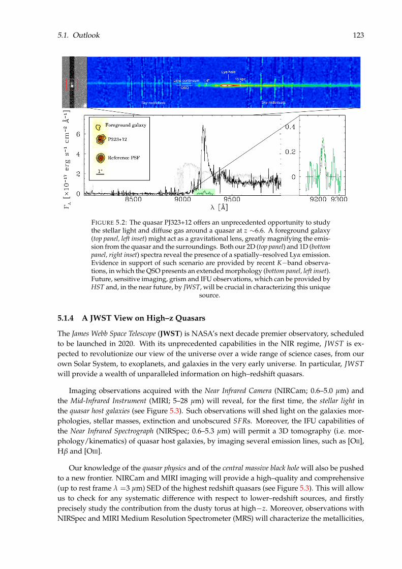
5.1. Outlook 123
FIGURE 5.2: The quasar PJ323+12 offers an unprecedented opportunity to studythe stellar light and diffuse gas around a quasar at z ∼6.6. A foreground galaxy(top panel, left inset) might act as a gravitational lens, greatly magnifying the emis-sion from the quasar and the surroundings. Both our 2D (top panel) and 1D (bottompanel, right inset) spectra reveal the presence of a spatially–resolved Lyα emission.Evidence in support of such scenario are provided by recent K−band observa-tions, in which the QSO presents an extended morphology (bottom panel, left inset).Future, sensitive imaging, grism and IFU observations, which can be provided byHST and, in the near future, by JWST, will be crucial in characterizing this unique
source.
5.1.4 A JWST View on High–z Quasars
The James Webb Space Telescope (JWST) is NASA’s next decade premier observatory, scheduledto be launched in 2020. With its unprecedented capabilities in the NIR regime, JWST is ex-pected to revolutionize our view of the universe over a wide range of science cases, from ourown Solar System, to exoplanets, and galaxies in the very early universe. In particular, JWSTwill provide a wealth of unparalleled information on high–redshift quasars.
Imaging observations acquired with the Near Infrared Camera (NIRCam; 0.6–5.0 µm) andthe Mid-Infrared Instrument (MIRI; 5–28 µm) will reveal, for the first time, the stellar light inthe quasar host galaxies (see Figure 5.3). Such observations will shed light on the galaxies mor-phologies, stellar masses, extinction and unobscured SFRs. Moreover, the IFU capabilities ofthe Near Infrared Spectrograph (NIRSpec; 0.6–5.3 µm) will permit a 3D tomography (i.e. mor-phology/kinematics) of quasar host galaxies, by imaging several emission lines, such as [OII],Hβ and [OIII].
Our knowledge of the quasar physics and of the central massive black hole will also be pushedto a new frontier. NIRCam and MIRI imaging will provide a high–quality and comprehensive(up to rest frame λ =3 µm) SED of the highest redshift quasars (see Figure 5.3). This will allowus to check for any systematic difference with respect to lower–redshift sources, and firstlyprecisely study the contribution from the dusty torus at high−z. Moreover, observations withNIRSpec and MIRI Medium Resolution Spectrometer (MRS) will characterize the metallicities,

124 Chapter 5. Conclusions and Outlook
FIGURE 5.3: Spectral Energy distribution of a quasar and its host galaxy atz =7.54. The broad band filter response curves of the NIRCam and MIRI camerason board JWST are overplotted. JWST will, for the first time at z >6, constrainthe entire UV-to-optical quasar’s SED, and it will pin down the contribution from
the stellar emission in the host galaxy.
kinematics and extinction of the BLRs, from the UV to the rest–frame optical regime. We willbe able to obtain precise black hole mass estimates from the Hβ emission line (e.g. Park et al.2012; see Sections 1.4.3 and 2.5.1). The simultaneous MBH measurements, using several broademission lines (e.g. CIV, MgII, Hβ, Hα), will inform us on whether the scaling relations/linecorrelations observed at lower−z still hold in the early universe (e.g. Shen et al. 2008).
The high S/N quasar spectra obtained with NIRSpec and MIRI MRS will also enable sys-tematic searches for metal absorption systems along the line of sight. These systems are essentialin the study of galaxy evolution, and in locating any emission from the first, metal–free Pop IIIstars (e.g. Becker et al. 2012, Kulkarni et al. 2013 and Ma et al. 2017). Complementary NIRSpecIFU and NIRCam imaging observations will permit the identification of the emitting counter-parts of the systems previously identified in absorption.
JWST offers exceptional tools to study the environment of high–redshift quasars. Analo-gously to quasars host galaxies, observations with NIRCam, NIRSpec and MIRI will unveilthe nature of the gas–rich companion galaxies to high−z quasars studied in Chapter 4, whoserest–frame optical stellar emission remains elusive so far. Moreover, NIRCam is equipped witha set of narrow band filters ideal to detect the Hα emission line at z ∼6.1-6.2. Two of thequasar+companion systems discovered by ALMA are located in within the filter response, to-gether with a large number of known quasars (see Figure 5.4). Thanks to observations witha combination of broad and narrow band filters, we will be able to characterize any ionizeddiffuse emission around the quasars and the companions, and to probe the larger scale envi-ronment by searching for Hα Emitters (HAE).

5.1. Outlook 125
Hα @ z=6.1JWST/NIRCAM
FIGURE 5.4: The JWST/NIRCam instrument offers a unique combination ofbroad and narrow band filters, thanks to which any emission from the quasarhosts or any companion galaxy will be detected. A number of known z ∼6.1quasars, and two quasar+companion systems (Decarli et al. 2017, see Chapter 4)
are located at suitable redshifts for such studies.
The unique capabilities of JWST will open a new, exciting window on the early universe,and will enable detailed and panchromatic investigations of massive galaxies and supermas-sive black holes in the first Gyr of cosmic history.


127
AcknowledgementsI wish to thank my supervisor, Fabian Walter, for his precious support, guidance and enthusi-asm through my PhD.
I would like to thank the members of Team HQ: Roberto Decarli, for your endless patience andsupport in me, in all aspects, from papers to proposals to future decisions; Emanuele Farina, forall the observing nights spent together, the scientific discussions (the pinky plot) and the meren-dellas; Eduardo Bañados, for sharing your (incredible!) knowledge of and passion for quasars;Bram Venemans, for patiently and kindly guiding me through data reduction/analysis anddatabase mining.
I thank Christian Fendt, our IMPRS coordinator, who, especially in the beginning of my PhD,helped me navigating the German and MPIA system. I also would like to thank my fellowmembers of the 10th IMPRS generation, for the nice time at the annual retreat(s) and the sup-portive feedback during our scientific activities.
I will never be able to deeply, wholeheartedly thank the many people that made my time inHeidelberg truly memorable.
I start by thanking the regular faces at “coffee after lunch”, Bert, Iskren, Morgan, Nikolay, Al-lison, for the shared coffee and laughter. I thank my officemates, Sara, Richard, Michael, Aiaraand Irina, for sharing with me the everyday life, including the hot summer days in the greenhouse. Thanks to Nadine, who always listened and encouraged me, and for simply being there,especially in the most difficult moments.
I thank the extended Gym(?) group: Peter, Gym tonight?; Reza, and his musical tastes; Christina,for all the scientific and psychological support; Maria, for your appreciation of my drivingskills, and because you always make me laugh, even in my particularly grumpy moments;Sara, I can’t even start to put in words how your very presence was essential for me; Thankyou for your time and your smile at volleyball, in the office, even at the hospital: I considermyself honored to be your friend.
I thank the “Italian Gang”: Gabriele and his jokes and great risotto; Laura, for the PS1 discus-sions, and the burger and chips nights; Chiara, for being an amazing person, for sustaining,understanding and hugging me when I truly needed; Alessandra, for our efficient shopping,for your patience, support, words of wisdom, and for helping me navigating through my para-noia: your support was crucial for me.
I thank my flatmate Anna, for the biscuits, ice cream, laughter and time with you and yourkind family: Thank you for being kind and supportive. I thank my volleyball team mates“Schnelleshelles”, because the time in the Gym was a ray of sunshine: Arjen, Sara, Arno, Ralph,Steffen, Claudia, Adrian, Laurent, Karin, Chrissi.
Finiró in italiano. Ringrazio i miei amici di sempre, della (ora!)gente che telegrammano: Bormio,Fulvio, Teo, Lucio, Marta, Carlo, Ricca, Carli. Nonostante i vari impegni, e il non costante con-tatto, le nostre cene/risottate mi fanno tornare indietro nel tempo. Ringrazio i “Panda”, Luca eFrancesca, perche’ ci conosciamo da piu di meta’ delle nostre vite, e il resto potete estrapolarlo.Ringrazio Nikita, perché il tuo sostegno, pratico e psicologico, e la tua presenza, mi hanno aiu-tato ad essere qui, e ad essere la persona che sono oggi.
Ringrazio la mia famiglia: i miei genitori, perche’ mi hanno supportata e sopportata sempre, e

128 Chapter 5. Conclusions and Outlook
i buongiorno e messaggi quotidiani sono stati per me piú importanti di quanto anche loro pos-sano pensare; mio fratello, per essere il mio riferimento informatico, per avermi incoraggiato eospitato, e sempre fatto ridere; Milena, per la tua dolcezza, i tuoi biscotti e il tuo sorriso; i mieinonni, che sono la mia bussola interna, qualsiasi cosa succeda.
Infine, come sempre, ringrazio te, Clara.

129
Appendix A
Filters Description
We list here in Table A.1 the broad band filters used throughout this work, both from publicsurveys and follow–up efforts.
TABLE A.1: List of broad band filters used in this thesis and their characteristics(Telescope/Survey, central wavelength and width).
Filter name Instrument/Survey λc ∆λ[µm] [µm]
gP1 PS1 0.487 0.117rP1 PS1 0.622 0.132iP1 PS1 0.755 0.124zP1 PS1 0.868 0.097yP1 PS1 0.963 0.062gdecam DECaLS 0.475 0.152rdecam DECaLS 0.640 0.143zdecam DECaLS 0.928 0.147R_SPECIAL VLT/FORS2 0.655 0.165z_GUNN VLT/FORS2 0.910 0.131FILT815_13+70 VLT/FORS2 0.815 0.13Y UKIDSS/VHS 1.000 0.120J UKIDSS/VHS 1.250 0.213H UKIDSS/VHS 1.650 0.307K UKIDSS/VHS 2.150 0.390zO2K CAHA 3.5m/Omega2000 0.908 0.158YO2K CAHA 3.5m/Omega2000 1.039 0.205JO2K CAHA 3.5m/Omega2000 1.234 0.164IE NTT/EFOSC2 0.793 0.126ZE NTT/EFOSC2 >0.840 −JS NTT/SofI 1.247 0.290iw CAHA 3.5m/CAFOS 0.762 0.139iMMT MMT/MMTCam 0.769 0.130Yretro su Pont/Retrocam 1.000 0.120JLUCI LBT/LUCI 1.247 0.305gG MPG 2.2m/GROND 0.459 0.137rG MPG 2.2m/GROND 0.622 0.156iG MPG 2.2m/GROND 0.764 0.094zG MPG 2.2m/GROND 0.899 0.128JG MPG 2.2m/GROND 1.240 0.229HG MPG 2.2m/GROND 1.647 0.264KG MPG 2.2m/GROND 2.171 0.303F105W HST/WFC3 1.0552 0.265F140W HST/WFC3 1.3923 0.384W1 ALLWISE 3.353 0.663W2 ALLWISE 4.603 1.042W3 ALLWISE 11.56 5.506[3.6] Spitzer/IRAC 3.550 0.750[4.5] Spitzer/IRAC 4.493 1.015[5.8] Spitzer/IRAC 5.731 1.425[8.0] Spitzer/IRAC 7.872 2.905


131
Appendix B
Spectroscopically Rejected Objects
We report in Table B.1 the Galactic contaminants found in our spectroscopic follow-up obser-vations, which satisfied our selection criteria considering the PS1 PV3 database information(three sources). We list names, coordinates, zP1 , yP1 , Y and J magnitudes. An accurate spectralclassification of the sources is beyond the scope of this work.
TABLE B.1: Objects spectroscopically confirmed to not be high redshift quasars.
Name R.A.(J2000) Decl. (J2000) zP1 yP1 Y J
PSO229.40365−22.37078 229.403651 -22.3707877 >22.36 20.36 ± 0.14 − 20.95 ± 0.27PSO267.27554+15.6457 267.2755422 15.64579622 22.48 ± 0.31 20.69 ± 0.13 − 20.31 ± 0.18PSO357.24231+25.77427 357.2423123 25.77427024 >22.81 20.72 ± 0.13 21.52 ±0.2 21.16 ± 0.14


133
Appendix C
Acronyms
AEGIS All-wavelength Extended Groth Strip International Survey
AGN Active Galactic Nucleus
ALLWISE all-sky Wide-field Infrared Survey Explorer
ALMA Atacama Large Millimeter Array
BAL Broad Absorption Line
BLR Broad Line Region
CFHQS Canada-France High-z Quasar Survey
COSMOS Cosmic Evolution Survey
CMB Cosmic Microwave Background
DBSP Double Spectrograph for the Palomar 200-inch Telescope
DeCALS Dark Energy Camera Legacy Survey
DES Dark Energy Survey
DLA Damped Lyman Alpha system
EFOSC2 ESO Faint Object Spectrograph and Camera 2
ESO European Southern Observatory
EoR Epoch of Reionization
EW Equivalent Width
FIR Far Infrared

134 Appendix C. Acronyms
FIRE Folded-port InfraRed Echellette
FORS2 FOcal Reducer/low dispersion Spectrograph 2
FOV Field of View
FWHM Full Width at Half Maximum
GOODS Great Observatories Origins Deep Survey
GNT Gemini North Telescope
GNIRS Gemini Near IR Spectrograph
GRB Gamma-Ray Burst
GROND Gamma-Ray Burst Optical Near-Infrared Detector
HAE Hα Emitters
HSC Hyper-Suprime Camera
HST Hubble Space Telescope
IGM Intergalactic Medium
IR Infrared
IRAC Infrared Array Camera for the Spitzer Space Telescope
IRAM Institute de Radioastronomie Millimétrique
ISM Interstellar Medium
JCMT James Clerk Maxwell Telescope
JWST James Webb Telescope
LAE Lyα Emitters
LBG Lyman Break Galaxies
LBT Large Binocular Telescope

Appendix C. Acronyms 135
LF Luminosity Function
LRIS Low Resolution Imaging Spectrometer
LSST Large Synoptic Survey Telescope
LUCI LBT Utility Camera in the Infrared
MMT Multiple Mirror Telescope
MODS Multi-Object Double Spectrograph
MPG Max Planck Gesellschaft
MUSE Multi Unit Spectrograph Explorer
NIR Near-Infrared
NOEMA NOrthern Extended Millimeter Array
NTT New Technology Telescope
Pan-STARRS1 Panoramic Survey Telescope & Rapid Response System 1PS1
PdBI Plateau de Bure Interferometer
PSF Point Spread Function
RM Reverberation Mapping
SDF Subaru Deep Field
SDF Spectral Energy Distribution
SDSS Sloan Digital Sky Survey
SFR Star Formation Rate
SMBH Supermassive Black Hole
SMG Submillimeter Galaxies

136 Appendix C. Acronyms
SN Supernova
SoFI infrared spectrograph and imaging camera Son of ISAAC
S/N Signal-to-noise ratio
TIR Total Infrared
UDS UKIDSS Ultra Deep Survey
UKIDSS UKIRT InfraRed Deep Sky Survey
UHS UKIRT Hemisphere Survey
ULIRG Ultra Luminous Infrared Galaxy
UV Ultraviolet
VHS VISTA Hemisphere Survey
VIKING Visible and Infrared Survey Telescope Kilo-Degree Infrared Galaxy
VISTA Visible and Infrared Survey Telescope for Astronomy
VLT Very Large Telescope
WEL Weak Emission Line
WFC3 Wide Field Camera 3
WFIRST Wide-Field Infrared Telescope
ΛCDM Lambda Cold Dark Matter

137
Bibliography
Ajiki, M. et al. (2006). “New Corroborative Evidence for the Overdensity of Galaxies around theRadio-Loud Quasar SDSS J0836+0054 at z = 5.8”. In: PASJ 58, pp. 499–502. DOI: 10.1093/pasj/58.3.499. eprint: astro-ph/0603298.
Alam, S. et al. (2015). “The Eleventh and Twelfth Data Releases of the Sloan Digital Sky Survey:Final Data from SDSS-III”. In: ApJS 219, 12, p. 12. DOI: 10.1088/0067-0049/219/1/12.arXiv: 1501.00963 [astro-ph.IM].
Alexander, T. and P. Natarajan (2014). “Rapid growth of seed black holes in the early universeby supra-exponential accretion”. In: Science 345, pp. 1330–1333. DOI: 10.1126/science.1251053. arXiv: 1408.1718.
Alvarez, M. A., J. H. Wise, and T. Abel (2009). “Accretion onto the First Stellar-Mass BlackHoles”. In: ApJL 701, pp. L133–L137. DOI: 10.1088/0004-637X/701/2/L133. arXiv: 0811.0820.
Amendola, L. et al. (2016). “Cosmology and Fundamental Physics with the Euclid Satellite”. In:ArXiv e-prints. arXiv: 1606.00180.
Angulo, R. E. et al. (2012). “The journey of QSO haloes from z ∼ 6 to the present”. In: MNRAS425, pp. 2722–2730. DOI: 10.1111/j.1365-2966.2012.21783.x. arXiv: 1203.5339.
Appenzeller, I. and G. Rupprecht (1992). “FORS - the focal reducer for the VLT.” In: The Mes-senger 67, pp. 18–21.
Appenzeller, I. et al. (1998). “Successful commissioning of FORS1 - the first optical instrumenton the VLT.” In: The Messenger 94, pp. 1–6.
Aravena, M. et al. (2016). “The ALMA Spectroscopic Survey in the Hubble Ultra Deep Field:Search for [CII] Line and Dust Emission in 6”. In: ApJ 833, 71, p. 71. DOI: 10.3847/1538-4357/833/1/71. arXiv: 1607.06772.
Armus, L. et al. (2009). “GOALS: The Great Observatories All-Sky LIRG Survey”. In: PASP 121,p. 559. DOI: 10.1086/600092. arXiv: 0904.4498.
Bañados, E. et al. (2013). “The Galaxy Environment of a QSO at z∼ 5.7”. In: ApJ 773, 178, p. 178.DOI: 10.1088/0004-637X/773/2/178. arXiv: 1306.6642 [astro-ph.CO].
Bañados, E. et al. (2014). “Discovery of Eight z∼ 6 Quasars from Pan-STARRS1”. In: AJ 148, 14,p. 14. DOI: 10.1088/0004-6256/148/1/14. arXiv: 1405.3986.
Bañados, E. et al. (2015a). “Bright [C II] 158 µm Emission in a Quasar Host Galaxy at z = 6.54”.In: ApJL 805, L8, p. L8. DOI: 10.1088/2041-8205/805/1/L8. arXiv: 1504.05216.
Bañados, E. et al. (2015b). “Constraining the Radio-loud Fraction of Quasars at z > 5.5”. In: ApJ804, 118, p. 118. DOI: 10.1088/0004-637X/804/2/118. arXiv: 1503.04214.
Bañados, E. et al. (2016). “The Pan-STARRS1 Distant z>5.6 Quasar Survey: More than 100Quasars within the First Gyr of the Universe”. In: ApJS 227, 11, p. 11. DOI: 10.3847/0067-0049/227/1/11. arXiv: 1608.03279.
Bañados, E. et al. (2018). “An 800-million-solar-mass black hole in a significantly neutral Uni-verse at a redshift of 7.5”. In: Nature 553, pp. 473–476. DOI: 10.1038/nature25180. arXiv:1712.01860.

138 BIBLIOGRAPHY
Baade, W. and R. Minkowski (1954). “Identification of the Radio Sources in Cassiopeia, CygnusA, and Puppis A.” In: ApJ 119, p. 206. DOI: 10.1086/145812.
Baan, W. A. and A. D. Haschick (1995). “Nuclear Antics of IC 4553 (ARP 220)”. In: ApJ 454,p. 745. DOI: 10.1086/176526.
Bailer-Jones, C. A., P. Bizenberger, and C. Storz (2000). “Achieving a wide-field near-infraredcamera for the Calar Alto 3.5-m telescope”. In: Optical and IR Telescope Instrumentation andDetectors. Ed. by M. Iye and A. F. Moorwood. Vol. 4008. PSPIE, pp. 1305–1316. DOI: 10.1117/12.395447. eprint: astro-ph/0003072.
Baldwin, J. A. (1977). “Luminosity Indicators in the Spectra of Quasi-Stellar Objects”. In: ApJ214, pp. 679–684. DOI: 10.1086/155294.
Balmaverde, B. et al. (2017). “Primordial environment of supermassive black holes. II. Deep Y-and J-band images around the z 6.3 quasar SDSS J1030+0524”. In: A&A 606, A23, A23. DOI:10.1051/0004-6361/201730683. arXiv: 1706.02317.
Barnett, R. et al. (2017). “Observations of the Lyman series forest towards the redshift 7.1 quasarULAS J1120+0641”. In: A&A 601, A16, A16. DOI: 10.1051/0004-6361/201630258. arXiv:1702.03687.
Barth, A. J. et al. (2003). “Iron Emission in the z = 6.4 Quasar SDSS J114816.64+525150.3”. In:ApJL 594, pp. L95–L98. DOI: 10.1086/378735. eprint: astro-ph/0308005.
Becker, G. D. et al. (2012). “Iron and α-element Production in the First One Billion Years afterthe Big Bang”. In: ApJ 744, 91, p. 91. DOI: 10.1088/0004-637X/744/2/91. arXiv: 1111.4843.
Becker, G. D. et al. (2015). “Evidence of patchy hydrogen reionization from an extreme Lyα
trough below redshift six”. In: MNRAS 447, pp. 3402–3419. DOI: 10.1093/mnras/stu2646.arXiv: 1407.4850.
Beelen, A. et al. (2006). “350 µm Dust Emission from High-Redshift Quasars”. In: ApJ 642,pp. 694–701. DOI: 10.1086/500636. eprint: astro-ph/0603121.
Begelman, M. C. and M. Volonteri (2017). “Hyperaccreting black holes in galactic nuclei”. In:MNRAS 464, pp. 1102–1107. DOI: 10.1093/mnras/stw2446. arXiv: 1609.07137 [astro-ph.HE].
Bentz, M. C. et al. (2013). “The Low-luminosity End of the Radius-Luminosity Relationship forActive Galactic Nuclei”. In: ApJ 767, 149, p. 149. DOI: 10.1088/0004- 637X/767/2/149.arXiv: 1303.1742.
Berta, S. et al. (2016). “Measures of galaxy dust and gas mass with Herschel photometry andprospects for ALMA”. In: A&A 587, A73, A73. DOI: 10.1051/0004-6361/201527746. arXiv:1511.05147.
Bertin, E. and S. Arnouts (1996). “SExtractor: Software for source extraction.” In: A&AS 117,pp. 393–404. DOI: 10.1051/aas:1996164.
Best, W. M. J. et al. (2013). “A Search for L/T Transition Dwarfs with Pan-STARRS1 and WISE:Discovery of Seven Nearby Objects Including Two Candidate Spectroscopic Variables”. In:ApJ 777, 84, p. 84. DOI: 10.1088/0004-637X/777/2/84. arXiv: 1309.0503 [astro-ph.SR].
Best, W. M. J. et al. (2015). “A Search for L/T Transition Dwarfs with Pan-STARRS1 and WISE.II. L/T Transition Atmospheres and Young Discoveries”. In: ApJ 814, 118, p. 118. DOI: 10.1088/0004-637X/814/2/118. arXiv: 1612.02824 [astro-ph.SR].
Bian, W.-H. and Y.-H. Zhao (2003). “Accretion Rates and the Accretion Efficiency in AGNs”. In:PASJ 55, pp. 599–603. DOI: 10.1093/pasj/55.3.599.
Blain, A. W. et al. (2002). “Submillimeter galaxies”. In: PhR 369, pp. 111–176. DOI: 10.1016/S0370-1573(02)00134-5. eprint: astro-ph/0202228.

BIBLIOGRAPHY 139
Bond, J. R., W. D. Arnett, and B. J. Carr (1984). “The evolution and fate of Very Massive Objects”.In: ApJ 280, pp. 825–847. DOI: 10.1086/162057.
Bondi, H. (1952). “On spherically symmetrical accretion”. In: MNRAS 112, p. 195. DOI: 10.1093/mnras/112.2.195.
Bouwens, R. J. et al. (2015a). “Reionization After Planck: The Derived Growth of the CosmicIonizing Emissivity Now Matches the Growth of the Galaxy UV Luminosity Density”. In:ApJ 811, 140, p. 140. DOI: 10.1088/0004-637X/811/2/140. arXiv: 1503.08228.
Bouwens, R. J. et al. (2015b). “UV Luminosity Functions at Redshifts z ∼ 4 to z ∼ 10: 10,000Galaxies from HST Legacy Fields”. In: ApJ 803, 34, p. 34. DOI: 10.1088/0004-637X/803/1/34. arXiv: 1403.4295.
Bowler, R. A. A. et al. (2015). “The galaxy luminosity function at z ' 6 and evidence for rapidevolution in the bright end from z ' 7 to 5”. In: MNRAS 452, pp. 1817–1840. DOI: 10.1093/mnras/stv1403. arXiv: 1411.2976.
Brammer, G. B., P. G. van Dokkum, and P. Coppi (2008). “EAZY: A Fast, Public PhotometricRedshift Code”. In: ApJ 686, 1503-1513, pp. 1503–1513. DOI: 10.1086/591786. arXiv: 0807.1533.
Brammer, G. B. et al. (2012). “3D-HST: A Wide-field Grism Spectroscopic Survey with the Hub-ble Space Telescope”. In: ApJS 200, 13, p. 13. DOI: 10.1088/0067-0049/200/2/13. arXiv:1204.2829.
Brenneman, L. W. et al. (2011). “The Spin of the Supermassive Black Hole in NGC 3783”. In: ApJ736, 103, p. 103. DOI: 10.1088/0004-637X/736/2/103. arXiv: 1104.1172 [astro-ph.HE].
Brinchmann, J. et al. (2004). “The physical properties of star-forming galaxies in the low-redshiftUniverse”. In: MNRAS 351, pp. 1151–1179. DOI: 10.1111/j.1365-2966.2004.07881.x.eprint: astro-ph/0311060.
Brisbin, D. et al. (2015). “Strong C+ Emission in Galaxies at z ∼ 1-2: Evidence for Cold FlowAccretion Powered Star Formation in the Early Universe”. In: ApJ 799, 13, p. 13. DOI: 10.1088/0004-637X/799/1/13. arXiv: 1411.1332.
Bruns, L. R. et al. (2012). “Clustering of Lyα emitters around luminous quasars at z= 2-3: analternative probe of reionization on galaxy formation”. In: MNRAS 421, pp. 2543–2552. DOI:10.1111/j.1365-2966.2012.20479.x. arXiv: 1105.3524.
Burgasser, A. J. (2014). “The SpeX Prism Library: 1000+ low-resolution, near-infrared spectraof ultracool M, L, T and Y dwarfs”. In: Astronomical Society of India Conference Series. Vol. 11.Astronomical Society of India Conference Series. arXiv: 1406.4887 [astro-ph.SR].
Buzzoni, B. et al. (1984). “The ESO Faint Object Spectrograph and Camera (EFOSC)”. In: TheMessenger 38, pp. 9–13.
Calderone, G. et al. (2017). “QSFIT: automatic analysis of optical AGN spectra”. In: MNRAS472, pp. 4051–4080. DOI: 10.1093/mnras/stx2239. arXiv: 1612.01580 [astro-ph.HE].
Calzetti, D. et al. (2000). “The Dust Content and Opacity of Actively Star-forming Galaxies”. In:ApJ 533, pp. 682–695. DOI: 10.1086/308692. eprint: astro-ph/9911459.
Capak, P. et al. (2004). “A Deep Wide-Field, Optical, and Near-Infrared Catalog of a Large Areaaround the Hubble Deep Field North”. In: AJ 127, pp. 180–198. DOI: 10.1086/380611. eprint:astro-ph/0312635.
Carilli, C. L. and F. Walter (2013). “Cool Gas in High-Redshift Galaxies”. In: ARA&A 51, pp. 105–161. DOI: 10.1146/annurev-astro-082812-140953. arXiv: 1301.0371.
Carilli, C. L. et al. (2010). “Ionization Near Zones Associated with Quasars at z ∼ 6”. In: ApJ714, pp. 834–839. DOI: 10.1088/0004-637X/714/1/834. arXiv: 1003.0016.

140 BIBLIOGRAPHY
Carnall, A. C. et al. (2015). “Two bright z > 6 quasars from VST ATLAS and a new method ofoptical plus mid-infrared colour selection”. In: MNRAS 451, pp. L16–L20. DOI: 10.1093/mnrasl/slv057. arXiv: 1502.07748.
Chambers, K. C. et al. (2016). “The Pan-STARRS1 Surveys”. In: ArXiv e-prints. arXiv: 1612.05560 [astro-ph.IM].
Chapman, S. C. et al. (2005). “A Redshift Survey of the Submillimeter Galaxy Population”. In:ApJ 622, pp. 772–796. DOI: 10.1086/428082. eprint: astro-ph/0412573.
Chehade, B. et al. (2018). “Two more, bright, z > 6 quasars from VST ATLAS and WISE”. In:MNRAS. DOI: 10.1093/mnras/sty690. arXiv: 1803.01424.
Chen, S.-F. S. et al. (2017). “Mg II Absorption at 2 < Z < 7 with Magellan/Fire. III. Full Statisticsof Absorption toward 100 High-redshift QSOs”. In: ApJ 850, 188, p. 188. DOI: 10.3847/1538-4357/aa9707. arXiv: 1612.02829.
Chiang, Y.-K., R. Overzier, and K. Gebhardt (2013). “Ancient Light from Young Cosmic Cities:Physical and Observational Signatures of Galaxy Proto-clusters”. In: ApJ 779, 127, p. 127.DOI: 10.1088/0004-637X/779/2/127. arXiv: 1310.2938.
Ciardi, B. and A. Ferrara (2005). “The First Cosmic Structures and Their Effects”. In: SSRv 116,pp. 625–705. DOI: 10.1007/s11214-005-3592-0. eprint: astro-ph/0409018.
Cool, R. J. et al. (2006). “The Discovery of Three New z>5 Quasars in the AGN and Galaxy Evo-lution Survey”. In: AJ 132, pp. 823–830. DOI: 10.1086/505535. eprint: astro-ph/0605030.
Cox, P. et al. (2011). “Gas and Dust in a Submillimeter Galaxy at z = 4.24 from the HerschelAtlas”. In: ApJ 740, 63, p. 63. DOI: 10.1088/0004-637X/740/2/63. arXiv: 1107.2924.
Croom, S. M. et al. (2005). “The 2dF QSO Redshift Survey - XIV. Structure and evolution fromthe two-point correlation function”. In: MNRAS 356, pp. 415–438. DOI: 10.1111/j.1365-2966.2004.08379.x. eprint: astro-ph/0409314.
da Cunha, E., S. Charlot, and D. Elbaz (2008). “A simple model to interpret the ultraviolet,optical and infrared emission from galaxies”. In: MNRAS 388, pp. 1595–1617. DOI: 10.1111/j.1365-2966.2008.13535.x. arXiv: 0806.1020.
da Cunha, E. et al. (2015). “An ALMA Survey of Sub-millimeter Galaxies in the Extended Chan-dra Deep Field South: Physical Properties Derived from Ultraviolet-to-radio Modeling”. In:ApJ 806, 110, p. 110. DOI: 10.1088/0004-637X/806/1/110. arXiv: 1504.04376.
Daddi, E. et al. (2007). “Multiwavelength Study of Massive Galaxies at z ∼ 2. I. Star Formationand Galaxy Growth”. In: ApJ 670, pp. 156–172. DOI: 10.1086/521818. arXiv: 0705.2831.
Davies, F. B. et al. (2018). “Quantitative Constraints on the Reionization History from the IGMDamping Wing Signature in Two Quasars at z > 7”. In: ArXiv e-prints. arXiv: 1802.06066.
Davis, M. and P. J. E. Peebles (1983). “A survey of galaxy redshifts. V - The two-point positionand velocity correlations”. In: ApJ 267, pp. 465–482. DOI: 10.1086/160884.
De Breuck, C. et al. (2011). “Enhanced [CII] emission in a z = 4.76 submillimetre galaxy”. In:A&A 530, L8, p. L8. DOI: 10.1051/0004-6361/201116868. arXiv: 1104.5250.
De Looze, I. et al. (2011). “The reliability of [C II] as an indicator of the star formation rate”. In:MNRAS 416, pp. 2712–2724. DOI: 10.1111/j.1365-2966.2011.19223.x. arXiv: 1106.1643[astro-ph.CO].
De Looze, I. et al. (2014). “The applicability of far-infrared fine-structure lines as star formationrate tracers over wide ranges of metallicities and galaxy types”. In: A&A 568, A62, A62. DOI:10.1051/0004-6361/201322489. arXiv: 1402.4075.
De Rosa, G. et al. (2011). “Evidence for Non-evolving Fe II/Mg II Ratios in Rapidly Accretingz ∼ 6 QSOs”. In: ApJ 739, 56, p. 56. DOI: 10.1088/0004-637X/739/2/56. arXiv: 1106.5501.

BIBLIOGRAPHY 141
De Rosa, G. et al. (2014). “Black Hole Mass Estimates and Emission-line Properties of a Sampleof Redshift z > 6.5 Quasars”. In: ApJ 790, 145, p. 145. DOI: 10.1088/0004-637X/790/2/145.arXiv: 1311.3260.
Decarli, R. et al. (2008). “On the geometry of broad emission region in quasars”. In: MNRAS387, pp. 1237–1247. DOI: 10.1111/j.1365-2966.2008.13320.x. arXiv: 0804.1875.
Decarli, R. et al. (2010). “The quasar MBH-Mhost relation through cosmic time - II. Evidencefor evolution from z = 3 to the present age”. In: MNRAS 402, pp. 2453–2461. DOI: 10.1111/j.1365-2966.2009.16049.x. arXiv: 0911.2988.
Decarli, R. et al. (2012). “Hubble Space Telescope Narrowband Search for Extended Lyα Emis-sion around Two z > 6 Quasars”. In: ApJ 756, 150, p. 150. DOI: 10.1088/0004-637X/756/2/150. arXiv: 1207.2155.
Decarli, R. et al. (2017). “Rapidly star-forming galaxies adjacent to quasars at redshifts exceed-ing 6”. In: Nature 545, pp. 457–461. DOI: 10.1038/nature22358. arXiv: 1705.08662.
— (2018). “An ALMA [C II] Survey of 27 Quasars at z > 5.94”. In: ApJ 854, 97, p. 97. DOI:10.3847/1538-4357/aaa5aa. arXiv: 1801.02641.
Degioia-Eastwood, K. et al. (1984). “Massive star formation in NGC 6946”. In: ApJ 278, pp. 564–574. DOI: 10.1086/161823.
Devecchi, B. and M. Volonteri (2009). “Formation of the First Nuclear Clusters and MassiveBlack Holes at High Redshift”. In: ApJ 694, pp. 302–313. DOI: 10.1088/0004-637X/694/1/302. arXiv: 0810.1057.
Díaz-Santos, T. et al. (2013). “Explaining the [C II]157.7 µm Deficit in Luminous Infrared Galaxies–First Results from a Herschel/PACS Study of the GOALS Sample”. In: ApJ 774, 68, p. 68.DOI: 10.1088/0004-637X/774/1/68. arXiv: 1307.2635.
Díaz-Santos, T. et al. (2017). “A Herschel/PACS Far-infrared Line Emission Survey of LocalLuminous Infrared Galaxies”. In: ApJ 846, 32, p. 32. DOI: 10.3847/1538- 4357/aa81d7.arXiv: 1705.04326.
Downes, D. and A. Eckart (2007). “Black hole in the West nucleus of Arp 220”. In: A&A 468,pp. L57–L61. DOI: 10.1051/0004-6361:20077301. arXiv: 0706.2599.
Downes, D. et al. (1992). “Submillimeter spectrum and dust mass of the primeval galaxy IRAS10214 + 4724”. In: ApJL 398, pp. L25–L27. DOI: 10.1086/186568.
Dubbeldam, M. et al. (2000). “Integral field unit for the Gemini near-infrared spectrograph”.In: Optical and IR Telescope Instrumentation and Detectors. Ed. by M. Iye and A. F. Moorwood.Vol. 4008. PSPIE, pp. 1181–1192. DOI: 10.1117/12.395437.
Dunlop, J. S. (2013). “Observing the First Galaxies”. In: The First Galaxies. Ed. by T. Wiklind,B. Mobasher, and V. Bromm. Vol. 396. Astrophysics and Space Science Library, p. 223. DOI:10.1007/978-3-642-32362-1_5. arXiv: 1205.1543.
Dunne, L., D. L. Clements, and S. A. Eales (2000). “Constraining the radio-submillimetre red-shift indicator using data from the SCUBA Local Universe Galaxy Survey”. In: MNRAS 319,pp. 813–820. DOI: 10.1046/j.1365-8711.2000.03882.x. eprint: astro-ph/0002436.
Edge, D. O. et al. (1959). “A survey of radio sources at a frequency of 159 Mc/s.” In: MmRAS68, pp. 37–60.
Eftekharzadeh, S. et al. (2015). “Clustering of intermediate redshift quasars using the final SDSSIII-BOSS sample”. In: MNRAS 453, pp. 2779–2798. DOI: 10.1093/mnras/stv1763. arXiv:1507.08380.

142 BIBLIOGRAPHY
Eilers, A.-C. et al. (2017). “Implications of z ∼ 6 Quasar Proximity Zones for the Epoch ofReionization and Quasar Lifetimes”. In: ApJ 840, 24, p. 24. DOI: 10.3847/1538-4357/aa6c60.arXiv: 1703.02539.
Engargiola, G. (1991). “Origins of the 12-200 micron flux in NGC 6946 - Starlight and continuumdust emission from an SC galaxy”. In: ApJS 76, pp. 875–910. DOI: 10.1086/191583.
Erben, T. et al. (2009). “CARS: the CFHTLS-Archive-Research Survey. I. Five-band multi-colourdata from 37 sq. deg. CFHTLS-wide observations”. In: A&A 493, pp. 1197–1222. DOI: 10.1051/0004-6361:200810426. arXiv: 0811.2239.
Fan, X., C. L. Carilli, and B. Keating (2006). “Observational Constraints on Cosmic Reioniza-tion”. In: ARA&A 44, pp. 415–462. DOI: 10.1146/annurev.astro.44.051905.092514.eprint: astro-ph/0602375.
Fan, X. et al. (2000). “The Discovery of a Luminous Z=5.80 Quasar from the Sloan Digital SkySurvey”. In: AJ 120, pp. 1167–1174. DOI: 10.1086/301534. eprint: astro-ph/0005414.
Fan, X. et al. (2003). “A Survey of z>5.7 Quasars in the Sloan Digital Sky Survey. II. Discovery ofThree Additional Quasars at z>6”. In: AJ 125, pp. 1649–1659. DOI: 10.1086/368246. eprint:astro-ph/0301135.
Fan, X. et al. (2006). “Constraining the Evolution of the Ionizing Background and the Epoch ofReionization with z∼6 Quasars. II. A Sample of 19 Quasars”. In: AJ 132, pp. 117–136. DOI:10.1086/504836. eprint: astro-ph/0512082.
Fanidakis, N. et al. (2012). “The evolution of active galactic nuclei across cosmic time: what isdownsizing?” In: MNRAS 419, pp. 2797–2820. DOI: 10.1111/j.1365-2966.2011.19931.x.arXiv: 1011.5222.
Fanidakis, N. et al. (2013). “The most luminous quasars do not live in the most massive darkmatter haloes at any redshift”. In: MNRAS 436, pp. 315–326. DOI: 10.1093/mnras/stt1567.arXiv: 1305.2199.
Farina, E. P. et al. (2017). “Mapping the Lyα Emission around a z ∼ 6.6 QSO with MUSE:Extended Emission and a Companion at a Close Separation”. In: ApJ 848, 78, p. 78. DOI:10.3847/1538-4357/aa8df4. arXiv: 1709.06096.
Farrah, D. et al. (2013). “Far-infrared Fine-structure Line Diagnostics of Ultraluminous InfraredGalaxies”. In: ApJ 776, 38, p. 38. DOI: 10.1088/0004-637X/776/1/38. arXiv: 1308.4165.
Fazio, G. G. et al. (2004). “The Infrared Array Camera (IRAC) for the Spitzer Space Telescope”.In: ApJS 154, pp. 10–17. DOI: 10.1086/422843. eprint: astro-ph/0405616.
Finkelstein, K. D. et al. (2015a). “Probing the Physical Properties of z = 4.5 Lyman Alpha Emit-ters with Spitzer”. In: ApJ 813, 78, p. 78. DOI: 10 . 1088 / 0004 - 637X / 813 / 1 / 78. arXiv:1509.06381.
Finkelstein, S. L. et al. (2009). “Lyman Alpha Galaxies: Primitive, Dusty, or Evolved?” In: ApJ691, pp. 465–481. DOI: 10.1088/0004-637X/691/1/465. arXiv: 0806.3269.
Finkelstein, S. L. et al. (2013). “A galaxy rapidly forming stars 700 million years after the BigBang at redshift 7.51”. In: Nature 502, pp. 524–527. DOI: 10.1038/nature12657. arXiv: 1310.6031.
Finkelstein, S. L. et al. (2015b). “The Evolution of the Galaxy Rest-frame Ultraviolet LuminosityFunction over the First Two Billion Years”. In: ApJ 810, 71, p. 71. DOI: 10 . 1088 / 0004 -637X/810/1/71. arXiv: 1410.5439.
Flewelling, H. A. et al. (2016). “The Pan-STARRS1 Database and Data Products”. In: ArXiv e-prints. arXiv: 1612.05243 [astro-ph.IM].

BIBLIOGRAPHY 143
Förster Schreiber, N. M. et al. (2003). “The Nature of Starburst Activity in M82”. In: ApJ 599,pp. 193–217. DOI: 10.1086/379097. eprint: astro-ph/0309357.
Fudamoto, Y. et al. (2017). “The most distant, luminous, dusty star-forming galaxies: redshiftsfrom NOEMA and ALMA spectral scans”. In: MNRAS 472, pp. 2028–2041. DOI: 10.1093/mnras/stx1956. arXiv: 1707.08967.
Fujimoto, S. et al. (2016). “ALMA Census of Faint 1.2 mm Sources Down to ∼ 0.02 mJy: Ex-tragalactic Background Light and Dust-poor, High-z Galaxies”. In: ApJS 222, 1, p. 1. DOI:10.3847/0067-0049/222/1/1. arXiv: 1505.03523.
Furlanetto, S. R. and S. P. Oh (2008). “The History and Morphology of Helium Reionization”.In: ApJ 681, 1-17, pp. 1–17. DOI: 10.1086/588546. arXiv: 0711.1542.
Furusawa, H. et al. (2008). “Subaru/XMM-Newton Deep Survey (SXDS) - Optical Imaging Sur-vey and Photometric Catalogs”. In: Panoramic Views of Galaxy Formation and Evolution. Ed.by T. Kodama, T. Yamada, and K. Aoki. Vol. 399. Astronomical Society of the Pacific Con-ference Series, p. 131.
Gaia Collaboration et al. (2016a). “Gaia Data Release 1. Summary of the astrometric, photomet-ric, and survey properties”. In: A&A 595, A2, A2. DOI: 10.1051/0004-6361/201629512.arXiv: 1609.04172 [astro-ph.IM].
Gaia Collaboration et al. (2016b). “The Gaia mission”. In: A&A 595, A1, A1. DOI: 10.1051/0004-6361/201629272. arXiv: 1609.04153 [astro-ph.IM].
Garel, T. et al. (2015). “The UV, Lyman α, and dark matter halo properties of high-redshiftgalaxies”. In: MNRAS 450, pp. 1279–1294. DOI: 10.1093/mnras/stv374. arXiv: 1503.06635.
Gehrels, N. (1986). “Confidence limits for small numbers of events in astrophysical data”. In:ApJ 303, pp. 336–346. DOI: 10.1086/164079.
Genzel, R., F. Eisenhauer, and S. Gillessen (2010). “The Galactic Center massive black holeand nuclear star cluster”. In: Reviews of Modern Physics 82, pp. 3121–3195. DOI: 10.1103/RevModPhys.82.3121. arXiv: 1006.0064.
Ghisellini, G., ed. (2013). Radiative Processes in High Energy Astrophysics. Vol. 873. Lecture Notesin Physics, Berlin Springer Verlag. DOI: 10.1007/978-3-319-00612-3. arXiv: 1202.5949[astro-ph.HE].
Giallongo, E. et al. (2015). “Faint AGNs at z > 4 in the CANDELS GOODS-S field: looking forcontributors to the reionization of the Universe”. In: A&A 578, A83, A83. DOI: 10.1051/0004-6361/201425334. arXiv: 1502.02562.
Gnedin, N. Y. (2000). “Effect of Reionization on Structure Formation in the Universe”. In: ApJ542, pp. 535–541. DOI: 10.1086/317042. eprint: astro-ph/0002151.
Gómez-Guijarro, C. et al. (2018). “Starburst to Quiescent from HST/ALMA: Stars and DustUnveil Minor Mergers in Submillimeter Galaxies at z ∼ 4.5”. In: ApJ 856, 121, p. 121. DOI:10.3847/1538-4357/aab206. arXiv: 1802.07751.
González, V. et al. (2011). “Evolution of Galaxy Stellar Mass Functions, Mass Densities, andMass-to-light Ratios from z ∼ 7 to z ∼ 4”. In: ApJL 735, L34, p. L34. DOI: 10.1088/2041-8205/735/2/L34. arXiv: 1008.3901.
Goto, T. et al. (2017). “No Ly α emitters detected around a QSO at z = 6.4: Suppressed by theQSO?” In: MNRAS 470, pp. L117–L121. DOI: 10.1093/mnrasl/slx088. arXiv: 1706.04620.
Graciá-Carpio, J. et al. (2011). “Far-infrared Line Deficits in Galaxies with Extreme L_FIR/M_H_2Ratios”. In: ApJL 728, L7, p. L7. DOI: 10.1088/2041-8205/728/1/L7. arXiv: 1101.0628.
Grandi, S. A. (1982). “The 3000 A bump in quasars”. In: ApJ 255, pp. 25–38. DOI: 10.1086/159799.

144 BIBLIOGRAPHY
Greenstein, J. L. (1963). “Red-Shift of the Unusual Radio Source: 3C 48”. In: Nature 197, pp. 1041–1042. DOI: 10.1038/1971041a0.
Greig, B. et al. (2017). “Are we witnessing the epoch of reionisation at z = 7.1 from the spectrumof J1120+0641?” In: MNRAS 466, pp. 4239–4249. DOI: 10.1093/mnras/stw3351. arXiv: 1606.00441.
Greiner, J. et al. (2008). “GROND–a 7-Channel Imager”. In: PASP 120, p. 405. DOI: 10.1086/587032. arXiv: 0801.4801.
Grier, C. J. et al. (2013). “The Structure of the Broad-line Region in Active Galactic Nuclei. I.Reconstructed Velocity-delay Maps”. In: ApJ 764, 47, p. 47. DOI: 10.1088/0004-637X/764/1/47. arXiv: 1210.2397.
Grier, C. J. et al. (2017). “The Sloan Digital Sky Survey Reverberation Mapping Project: Hα andHβ Reverberation Measurements from First-year Spectroscopy and Photometry”. In: ApJ851, 21, p. 21. DOI: 10.3847/1538-4357/aa98dc. arXiv: 1711.03114.
Gullberg, B. et al. (2015). “The nature of the [C II] emission in dusty star-forming galaxies fromthe SPT survey”. In: MNRAS 449, pp. 2883–2900. DOI: 10.1093/mnras/stv372. arXiv: 1501.06909.
Haehnelt, M. G. and M. J. Rees (1993). “The formation of nuclei in newly formed galaxies andthe evolution of the quasar population”. In: MNRAS 263, pp. 168–178. DOI: 10.1093/mnras/263.1.168.
Hashimoto, T. et al. (2013). “Gas Motion Study of Lyα Emitters at z ∼ 2 Using FUV and OpticalSpectral Lines”. In: ApJ 765, 70, p. 70. DOI: 10.1088/0004-637X/765/1/70. arXiv: 1206.2316.
Hazard, C., M. B. Mackey, and A. J. Shimmins (1963). “Investigation of the Radio Source 3C273 By The Method of Lunar Occultations”. In: Nature 197, pp. 1037–1039. DOI: 10.1038/1971037a0.
Hazard, C. et al. (2018). “The Sequence of Events that led to the 1963 Publications in Nature of3C 273, the First Quasar and the First Extragalactic Radio Jet”. In: PASA 35, e006, e006. DOI:10.1017/pasa.2017.62.
Helou, G. et al. (1988). “IRAS observations of galaxies in the Virgo cluster area”. In: ApJS 68,pp. 151–172. DOI: 10.1086/191285.
Hennawi, J. F. et al. (2006). “Binary Quasars in the Sloan Digital Sky Survey: Evidence for ExcessClustering on Small Scales”. In: AJ 131, pp. 1–23. DOI: 10.1086/498235. eprint: astro-ph/0504535.
Hennawi, J. F. et al. (2015). “Quasar quartet embedded in giant nebula reveals rare massivestructure in distant universe”. In: Science 348, pp. 779–783. DOI: 10.1126/science.aaa5397.arXiv: 1505.03786.
Herrera-Camus, R. et al. (2015). “[C II] 158 µm Emission as a Star Formation Tracer”. In: ApJ800, 1, p. 1. DOI: 10.1088/0004-637X/800/1/1. arXiv: 1409.7123.
Herrera-Camus, R. et al. (2018). “SHINING, A Survey of Far Infrared Lines in Nearby Galax-ies. I: Survey Description, Observational Trends, and Line Diagnostics”. In: ArXiv e-prints.arXiv: 1803.04419.
Hildebrandt, H. et al. (2009). “CARS: the CFHTLS-Archive-Research Survey. II. Weighing darkmatter halos of Lyman-break galaxies at z = 3-5”. In: A&A 498, pp. 725–736. DOI: 10.1051/0004-6361/200811042. arXiv: 0903.3951.
Hodge, J. A. et al. (2013). “An ALMA Survey of Submillimeter Galaxies in the Extended Chan-dra Deep Field South: Source Catalog and Multiplicity”. In: ApJ 768, 91, p. 91. DOI: 10.1088/0004-637X/768/1/91. arXiv: 1304.4266.

BIBLIOGRAPHY 145
Hopkins, P. F. et al. (2008). “A Cosmological Framework for the Co-Evolution of Quasars, Su-permassive Black Holes, and Elliptical Galaxies. I. Galaxy Mergers and Quasar Activity”.In: ApJS 175, 356-389, pp. 356–389. DOI: 10.1086/524362. arXiv: 0706.1243.
Hu, E. M. et al. (2010). “An Atlas of z = 5.7 and z = 6.5 Lyα Emitters”. In: ApJ 725, pp. 394–423.DOI: 10.1088/0004-637X/725/1/394. arXiv: 1009.1144.
Hubble, E. (1929). “A Relation between Distance and Radial Velocity among Extra-GalacticNebulae”. In: Proceedings of the National Academy of Science 15, pp. 168–173. DOI: 10.1073/pnas.15.3.168.
Hughes, D. H. et al. (1998). “High-redshift star formation in the Hubble Deep Field revealedby a submillimetre-wavelength survey”. In: Nature 394, pp. 241–247. DOI: 10.1038/28328.eprint: astro-ph/9806297.
Husband, K. et al. (2013). “Are z ∼ 5 quasars found in the most massive high-redshift overden-sities?” In: MNRAS 432, pp. 2869–2877. DOI: 10.1093/mnras/stt642. arXiv: 1304.3726.
Ivezic, Z. et al. (2008). “LSST: from Science Drivers to Reference Design and Anticipated DataProducts”. In: ArXiv e-prints. arXiv: 0805.2366.
Ivezic, Ž. et al. (2014). “Optical selection of quasars: SDSS and LSST”. In: Multiwavelength AGNSurveys and Studies. Ed. by A. M. Mickaelian and D. B. Sanders. Vol. 304. IAU Symposium,pp. 11–17. DOI: 10.1017/S1743921314003159. arXiv: 1312.3963 [astro-ph.IM].
Ivison, R. J. et al. (2000). “The diversity of SCUBA-selected galaxies”. In: MNRAS 315, pp. 209–222. DOI: 10.1046/j.1365-8711.2000.03376.x. eprint: astro-ph/9911069.
Ivison, R. J. et al. (2010). “Herschel and SCUBA-2 imaging and spectroscopy of a bright, lensedsubmillimetre galaxy at z = 2.3”. In: A&A 518, L35, p. L35. DOI: 10.1051/0004- 6361/201014548. arXiv: 1005.1071.
Iwamuro, F. et al. (2002). “Fe II/Mg II Emission-Line Ratios of QSOs within 0 < z < 5.3”. In:ApJ 565, pp. 63–77. DOI: 10.1086/324540.
Iwamuro, F. et al. (2004). “Fe II/Mg II Emission-Line Ratios of QSOs. II. z > 6 Objects”. In: ApJ614, pp. 69–74. DOI: 10.1086/423610. eprint: astro-ph/0408517.
Jiang, L. et al. (2007). “Gemini Near-Infrared Spectroscopy of Luminous z ∼ 6 Quasars: Chem-ical Abundances, Black Hole Masses, and Mg II Absorption”. In: AJ 134, p. 1150. DOI: 10.1086/520811. arXiv: 0707.1663.
Jiang, L. et al. (2016). “The Final SDSS High-redshift Quasar Sample of 52 Quasars at z>5.7”.In: ApJ 833, 222, p. 222. DOI: 10.3847/1538-4357/833/2/222. arXiv: 1610.05369.
Joseph, R. D. and G. S. Wright (1985). “Recent star formation in interacting galaxies. II - Superstarburst in merging galaxies”. In: MNRAS 214, pp. 87–95. DOI: 10.1093/mnras/214.2.87.
Kaiser, N. et al. (2002). “Pan-STARRS: A Large Synoptic Survey Telescope Array”. In: Surveyand Other Telescope Technologies and Discoveries. Ed. by J. A. Tyson and S. Wolff. Vol. 4836.PSPIE, pp. 154–164. DOI: 10.1117/12.457365.
Kaiser, N. et al. (2010). “The Pan-STARRS wide-field optical/NIR imaging survey”. In: Ground-based and Airborne Telescopes III. Vol. 7733. PSPIE, 77330E. DOI: 10.1117/12.859188.
Kashikawa, N. et al. (2015). “The Subaru High-z Quasar Survey: Discovery of Faint z ∼ 6Quasars”. In: ApJ 798, 28, p. 28. DOI: 10.1088/0004-637X/798/1/28. arXiv: 1410.7401.
Kaspi, S. et al. (2005). “The Relationship between Luminosity and Broad-Line Region Size inActive Galactic Nuclei”. In: ApJ 629, pp. 61–71. DOI: 10.1086/431275. eprint: astro-ph/0504484.

146 BIBLIOGRAPHY
Kawamata, R. et al. (2016). “Precise Strong Lensing Mass Modeling of Four Hubble FrontierField Clusters and a Sample of Magnified High-redshift Galaxies”. In: ApJ 819, 114, p. 114.DOI: 10.3847/0004-637X/819/2/114. arXiv: 1510.06400.
Kellermann, K. I. et al. (1989). “VLA observations of objects in the Palomar Bright Quasar Sur-vey”. In: AJ 98, pp. 1195–1207. DOI: 10.1086/115207.
Kennicutt, R. C. and N. J. Evans (2012). “Star Formation in the Milky Way and Nearby Galax-ies”. In: ARA&A 50, pp. 531–608. DOI: 10.1146/annurev-astro-081811-125610. arXiv:1204.3552.
Kim, S. et al. (2009). “The Environments of High-Redshift Quasi-Stellar Objects”. In: ApJ 695,pp. 809–817. DOI: 10.1088/0004-637X/695/2/809. arXiv: 0805.1412.
Kim, Y. et al. (2015). “Discovery of a Faint Quasar at z ∼ 6 and Implications for Cosmic Reion-ization”. In: ApJL 813, L35, p. L35. DOI: 10.1088/2041-8205/813/2/L35. arXiv: 1511.01585.
Kovac, K. et al. (2007). “Clustering of Lyα Emitters at z ∼ 4.5”. In: ApJ 668, pp. 15–22. DOI:10.1086/520668. arXiv: 0706.0893.
Kulkarni, G. et al. (2013). “Chemical Enrichment of Damped Lyα Systems as a Direct Constrainton Population III Star Formation”. In: ApJ 772, 93, p. 93. DOI: 10.1088/0004-637X/772/2/93.arXiv: 1301.4201.
Kurk, J. D. et al. (2007). “Black Hole Masses and Enrichment of z ∼ 6 SDSS Quasars”. In: ApJ669, pp. 32–44. DOI: 10.1086/521596. arXiv: 0707.1662.
Kurk, J. D. et al. (2009). “Near-Infrared Spectroscopy of SDSS J0303 - 0019: A Low-luminosity,High-Eddington-Ratio Quasar at z ∼ 6”. In: ApJ 702, pp. 833–837. DOI: 10.1088/0004-637X/702/2/833. arXiv: 0907.0435.
Lang, D. (2014). “unWISE: Unblurred Coadds of the WISE Imaging”. In: AJ 147, 108, p. 108.DOI: 10.1088/0004-6256/147/5/108. arXiv: 1405.0308 [astro-ph.IM].
Lang, D. et al. (2010). “Astrometry.net: Blind Astrometric Calibration of Arbitrary AstronomicalImages”. In: AJ 139, pp. 1782–1800. DOI: 10.1088/0004-6256/139/5/1782. arXiv: 0910.2233[astro-ph.IM].
Langer, W. D. and J. L. Pineda (2015). “[C ii] emission from galactic nuclei in the presence ofX-rays”. In: A&A 580, A5, A5. DOI: 10.1051/0004-6361/201525950. arXiv: 1505.02777.
Lapi, A. et al. (2006). “Quasar Luminosity Functions from Joint Evolution of Black Holes andHost Galaxies”. In: ApJ 650, pp. 42–56. DOI: 10.1086/507122. eprint: astro-ph/0603819.
Latif, M. A. and A. Ferrara (2016). “Formation of Supermassive Black Hole Seeds”. In: PASA33, e051, e051. DOI: 10.1017/pasa.2016.41. arXiv: 1605.07391.
Latif, M. A. and D. R. G. Schleicher (2015). “The formation of supermassive black holes inrapidly rotating disks”. In: A&A 578, A118, A118. DOI: 10.1051/0004-6361/201525855.arXiv: 1411.5902.
Laureijs, R. et al. (2011). “Euclid Definition Study Report”. In: ArXiv e-prints. arXiv: 1110.3193[astro-ph.CO].
Lawrence, A. et al. (2007). “The UKIRT Infrared Deep Sky Survey (UKIDSS)”. In: MNRAS 379,pp. 1599–1617. DOI: 10.1111/j.1365-2966.2007.12040.x. eprint: astro-ph/0604426.
Leighly, K. M. (2004). “Hubble Space Telescope STIS Ultraviolet Spectral Evidence of Outflowin Extreme Narrow-Line Seyfert 1 Galaxies. II. Modeling and Interpretation”. In: ApJ 611,pp. 125–152. DOI: 10.1086/422089. eprint: astro-ph/0402452.
Leipski, C. et al. (2014). “Spectral Energy Distributions of QSOs at z > 5: Common ActiveGalactic Nucleus-heated Dust and Occasionally Strong Star-formation”. In: ApJ 785, 154,p. 154. DOI: 10.1088/0004-637X/785/2/154. arXiv: 1402.5976.
BIBLIOGRAPHY 147
Leroy, A. K. et al. (2017). “Cloud-scale ISM Structure and Star Formation in M51”. In: ApJ 846,71, p. 71. DOI: 10.3847/1538-4357/aa7fef. arXiv: 1706.08540.
Lira, P. et al. (2018). “Reverberation Mapping of High-z, High-luminosity Quasars”. In: Frontiersin Astronomy and Space Sciences 4, 71, p. 71. DOI: 10.3389/fspas.2017.00071. arXiv: 1801.03866.
Lodieu, N., S. Boudreault, and V. J. S. Béjar (2014). “Spectroscopy of Hyades L dwarf candi-dates”. In: MNRAS 445, pp. 3908–3918. DOI: 10.1093/mnras/stu2059. arXiv: 1410.0192[astro-ph.SR].
Loeb, A. and R. Barkana (2001). “The Reionization of the Universe by the First Stars andQuasars”. In: ARA&A 39, pp. 19–66. DOI: 10.1146/annurev.astro.39.1.19. eprint: astro-ph/0010467.
Longair, M. S. (2008). Galaxy Formation.LSST Science Collaboration et al. (2009). “LSST Science Book, Version 2.0”. In: ArXiv e-prints.
arXiv: 0912.0201 [astro-ph.IM].Lupi, A. et al. (2016). “Growing massive black holes through supercritical accretion of stellar-
mass seeds”. In: MNRAS 456, pp. 2993–3003. DOI: 10.1093/mnras/stv2877. arXiv: 1512.02651.
Ma, Q. et al. (2017). “Metal enrichment signatures of the first stars on high-z DLAs”. In: MNRAS472, pp. 3532–3542. DOI: 10.1093/mnras/stx1839. arXiv: 1707.07580.
Mace, G. N. (2014). “Investigating Low-Mass Binary Stars And Brown Dwarfs with Near-Infrared Spectroscopy”. PhD thesis. University of California, Los Angeles.
Madau, P., F. Haardt, and M. Dotti (2014). “Super-critical Growth of Massive Black Holes fromStellar-mass Seeds”. In: ApJL 784, L38, p. L38. DOI: 10.1088/2041-8205/784/2/L38. arXiv:1402.6995.
Magdis, G. E. et al. (2011). “GOODS-Herschel: Gas-to-dust Mass Ratios and CO-to-H2 Conver-sion Factors in Normal and Starbursting Galaxies at High-z”. In: ApJL 740, L15, p. L15. DOI:10.1088/2041-8205/740/1/L15. arXiv: 1109.1140.
Magnier, E. A. et al. (2013). “The Pan-STARRS 1 Photometric Reference Ladder, Release 12.01”.In: ApJS 205, 20, p. 20. DOI: 10.1088/0067-0049/205/2/20. arXiv: 1303.3634 [astro-ph.IM].
Magnier, E. A. et al. (2016). “The Pan-STARRS Data Processing System”. In: ArXiv e-prints.arXiv: 1612.05240 [astro-ph.IM].
Mainzer, A. et al. (2011). “Preliminary Results from NEOWISE: An Enhancement to the Wide-field Infrared Survey Explorer for Solar System Science”. In: ApJ 731, 53, p. 53. DOI: 10.1088/0004-637X/731/1/53. arXiv: 1102.1996 [astro-ph.EP].
Maiolino, R. et al. (2003). “Early Star Formation Traced by the Highest Redshift Quasars”. In:ApJL 596, pp. L155–L158. DOI: 10.1086/379600. eprint: astro-ph/0307264.
Maiolino, R. et al. (2005). “First detection of [CII]158 µm at high redshift: vigorous star forma-tion in the early universe”. In: A&A 440, pp. L51–L54. DOI: 10.1051/0004-6361:200500165.eprint: astro-ph/0508064.
Maiolino, R. et al. (2009). “Strong [CII] emission at high redshift”. In: A&A 500, pp. L1–L4. DOI:10.1051/0004-6361/200912265. arXiv: 0904.3793.
Malhotra, S. et al. (2001). “Far-Infrared Spectroscopy of Normal Galaxies: Physical Conditionsin the Interstellar Medium”. In: ApJ 561, pp. 766–786. DOI: 10.1086/323046. eprint: astro-ph/0106485.

148 BIBLIOGRAPHY
Marconi, A. et al. (2008). “The Effect of Radiation Pressure on Virial Black Hole Mass Estimatesand the Case of Narrow-Line Seyfert 1 Galaxies”. In: ApJ 678, 693-700, pp. 693–700. DOI:10.1086/529360. arXiv: 0802.2021.
Marocco, F. et al. (2015). “A large spectroscopic sample of L and T dwarfs from UKIDSS LAS:peculiar objects, binaries, and space density”. In: MNRAS 449, pp. 3651–3692. DOI: 10.1093/mnras/stv530. arXiv: 1503.05082 [astro-ph.SR].
Marrone, D. P. et al. (2018). “Galaxy growth in a massive halo in the first billion years of cosmichistory”. In: Nature 553, pp. 51–54. DOI: 10.1038/nature24629. arXiv: 1712.03020.
Matsuoka, Y. et al. (2016). “Subaru High-z Exploration of Low-luminosity Quasars (SHELLQs).I. Discovery of 15 Quasars and Bright Galaxies at 5.7 < z < 6.9”. In: ApJ 828, 26, p. 26. DOI:10.3847/0004-637X/828/1/26. arXiv: 1603.02281.
Matsuoka, Y. et al. (2018a). “Subaru High-z Exploration of Low-Luminosity Quasars (SHEL-LQs). II. Discovery of 32 quasars and luminous galaxies at 5.7 < z ≤ 6.8”. In: PASJ 70, S35,S35. DOI: 10.1093/pasj/psx046. arXiv: 1704.05854.
Matsuoka, Y. et al. (2018b). “Subaru High-z Exploration of Low-Luminosity Quasars (SHEL-LQs). IV. Discovery of 41 Quasars and Luminous Galaxies at 5.7 < z < 6.9”. In: ArXiv e-prints. arXiv: 1803.01861.
Matteucci, F. and L. Greggio (1986). “Relative roles of type I and II supernovae in the chemicalenrichment of the interstellar gas”. In: A&A 154, pp. 279–287.
Matthews, J. H., C. Knigge, and K. S. Long (2017). “Quasar emission lines as probes of orien-tation: implications for disc wind geometries and unification”. In: MNRAS 467, pp. 2571–2584. DOI: 10.1093/mnras/stx231. arXiv: 1701.07037.
Mazzucchelli, C. et al. (2017a). “No Overdensity of Lyman-Alpha Emitting Galaxies arounda Quasar at z ∼ 5.7”. In: ApJ 834, 83, p. 83. DOI: 10.3847/1538-4357/834/1/83. arXiv:1611.02870.
Mazzucchelli, C. et al. (2017b). “Physical Properties of 15 Quasars at z & 6.5”. In: ApJ 849, 91,p. 91. DOI: 10.3847/1538-4357/aa9185. arXiv: 1710.01251.
McGreer, I. D., A. Mesinger, and V. D’Odorico (2015). “Model-independent evidence in favourof an end to reionization by z ≈ 6”. In: MNRAS 447, pp. 499–505. DOI: 10.1093/mnras/stu2449. arXiv: 1411.5375.
McGreer, I. D. et al. (2006). “Discovery of a z = 6.1 Radio-Loud Quasar in the NOAO Deep WideField Survey”. In: ApJ 652, pp. 157–162. DOI: 10.1086/507767. eprint: astro-ph/0607278.
McGreer, I. D. et al. (2014). “Close Companions to Two High-redshift Quasars”. In: AJ 148, 73,p. 73. DOI: 10.1088/0004-6256/148/4/73. arXiv: 1404.2297.
McGreer, I. D. et al. (2016). “A Constraint on Quasar Clustering at z = 5 from a Binary Quasar”.In: AJ 151, 61, p. 61. DOI: 10.3847/0004-6256/151/3/61. arXiv: 1601.03056.
McLeod, D. J. et al. (2015). “New redshift z ' 9 galaxies in the Hubble Frontier Fields: impli-cations for early evolution of the UV luminosity density”. In: MNRAS 450, pp. 3032–3044.DOI: 10.1093/mnras/stv780. arXiv: 1412.1472.
McMahon, R. G. et al. (2013). “First Scientific Results from the VISTA Hemisphere Survey(VHS)”. In: The Messenger 154, pp. 35–37.
McQuinn, M. (2016). “The Evolution of the Intergalactic Medium”. In: ARA&A 54, pp. 313–362.DOI: 10.1146/annurev-astro-082214-122355. arXiv: 1512.00086.
Mechtley, M. et al. (2012). “Near-infrared Imaging of a z = 6.42 Quasar Host Galaxy with theHubble Space Telescope Wide Field Camera 3”. In: ApJL 756, L38, p. L38. DOI: 10.1088/2041-8205/756/2/L38. arXiv: 1207.3283 [astro-ph.CO].

BIBLIOGRAPHY 149
Meiksin, A. (2006). “Colour corrections for high-redshift objects due to intergalactic attenua-tion”. In: MNRAS 365, pp. 807–812. DOI: 10.1111/j.1365-2966.2005.09756.x. eprint:astro-ph/0512435.
Meisner, A. M., D. Lang, and D. J. Schlegel (2016). “Full-depth Coadds of the WISE and NEOWISE-Reactivation Data”. In: American Astronomical Society Meeting Abstracts #227. Vol. 227. Amer-ican Astronomical Society Meeting Abstracts, p. 140.03.
Mesinger, A. (2018). “Reionization and Cosmic Dawn: theory and simulations”. In: ArXiv e-prints. arXiv: 1801.02649.
Miralda-Escudé, J. (1998). “Reionization of the Intergalactic Medium and the Damping Wingof the Gunn-Peterson Trough”. In: ApJ 501, pp. 15–22. DOI: 10.1086/305799. eprint: astro-ph/9708253.
Miyoshi, M. et al. (1995). “Evidence for a black hole from high rotation velocities in a sub-parsecregion of NGC4258”. In: Nature 373, pp. 127–129. DOI: 10.1038/373127a0.
Moorwood, A., J.-G. Cuby, and C. Lidman (1998). “SOFI sees first light at the NTT.” In: TheMessenger 91, pp. 9–13.
Morganson, E. et al. (2012). “The First High-redshift Quasar from Pan-STARRS”. In: AJ 143,142, p. 142. DOI: 10.1088/0004-6256/143/6/142. arXiv: 1109.6241.
Morselli, L. et al. (2014). “Primordial environment of super massive black holes: large-scalegalaxy overdensities around z ∼ 6 quasars with LBT”. In: A&A 568, A1, A1. DOI: 10.1051/0004-6361/201423853. arXiv: 1406.3961.
Mortlock, D. J. et al. (2009). “Discovery of a redshift 6.13 quasar in the UKIRT infrared deep skysurvey”. In: A&A 505, pp. 97–104. DOI: 10.1051/0004-6361/200811161. arXiv: 0810.4180.
Mortlock, D. J. et al. (2011). “A luminous quasar at a redshift of z = 7.085”. In: Nature 474,pp. 616–619. DOI: 10.1038/nature10159. arXiv: 1106.6088 [astro-ph.CO].
Muldrew, S. I., N. A. Hatch, and E. A. Cooke (2015). “What are protoclusters? - Defining high-redshift galaxy clusters and protoclusters”. In: MNRAS 452, pp. 2528–2539. DOI: 10.1093/mnras/stv1449. arXiv: 1506.08835.
Murphy, E. J. et al. (2011). “Calibrating Extinction-free Star Formation Rate Diagnostics with 33GHz Free-free Emission in NGC 6946”. In: ApJ 737, 67, p. 67. DOI: 10.1088/0004-637X/737/2/67. arXiv: 1105.4877.
Namikawa, T. (2018). “Constraints on patchy reionization from Planck CMB temperature trispec-trum”. In: PhRvD 97.6, 063505, p. 063505. DOI: 10.1103/PhysRevD.97.063505. arXiv: 1711.00058.
Noeske, K. G. et al. (2007). “Star Formation in AEGIS Field Galaxies since z=1.1: The Dominanceof Gradually Declining Star Formation, and the Main Sequence of Star-forming Galaxies”.In: ApJL 660, pp. L43–L46. DOI: 10.1086/517926. eprint: astro-ph/0701924.
Nomoto, K. et al. (1997). “Nucleosynthesis in type II supernovae”. In: Nuclear Physics A 616,pp. 79–90. DOI: 10.1016/S0375-9474(97)00076-6. eprint: astro-ph/9706024.
Oesch, P. A. et al. (2016). “A Remarkably Luminous Galaxy at z=11.1 Measured with HubbleSpace Telescope Grism Spectroscopy”. In: ApJ 819, 129, p. 129. DOI: 10.3847/0004-637X/819/2/129. arXiv: 1603.00461.
Oke, J. B. and J. E. Gunn (1982). “An Efficient Low Resolution and Moderate Resolution Spec-trograph for the Hale Telescope”. In: PASP 94, p. 586. DOI: 10.1086/131027.
Oke, J. B. et al. (1995). “The Keck Low-Resolution Imaging Spectrometer”. In: PASP 107, p. 375.DOI: 10.1086/133562.

150 BIBLIOGRAPHY
Onken, C. A. et al. (2004). “Supermassive Black Holes in Active Galactic Nuclei. II. Calibrationof the Black Hole Mass-Velocity Dispersion Relationship for Active Galactic Nuclei”. In: ApJ615, pp. 645–651. DOI: 10.1086/424655. eprint: astro-ph/0407297.
Ono, Y. et al. (2010). “Stellar Populations of Lyα Emitters at z ∼ 6-7: Constraints on the EscapeFraction of Ionizing Photons from Galaxy Building Blocks”. In: ApJ 724, pp. 1524–1535. DOI:10.1088/0004-637X/724/2/1524. arXiv: 1004.0963.
Ono, Y. et al. (2012). “Spectroscopic Confirmation of Three z-dropout Galaxies at z = 6.844-7.213:Demographics of Lyα Emission in z∼ 7 Galaxies”. In: ApJ 744, 83, p. 83. DOI: 10.1088/0004-637X/744/2/83. arXiv: 1107.3159.
Osterbrock, D. E. (1989). Astrophysics of gaseous nebulae and active galactic nuclei.Ota, K. et al. (2018). “Large Scale Environment of a z = 6.61 Luminous Quasar Probed by Lyα
Emitters and Lyman Break Galaxies”. In: ArXiv e-prints. arXiv: 1802.08912.Ouchi, M. et al. (2003). “Subaru Deep Survey. II. Luminosity Functions and Clustering Prop-
erties of Lyα Emitters at z=4.86 in the Subaru Deep Field”. In: ApJ 582, pp. 60–68. DOI:10.1086/344476. eprint: astro-ph/0202204.
Ouchi, M. et al. (2008). “The Subaru/XMM-Newton Deep Survey (SXDS). IV. Evolution of Lyα
Emitters from z = 3.1 to 5.7 in the 1 deg2 Field: Luminosity Functions and AGN”. In: ApJS176, 301-330, pp. 301–330. DOI: 10.1086/527673. arXiv: 0707.3161.
Ouchi, M. et al. (2018). “Systematic Identification of LAEs for Visible Exploration and Reion-ization Research Using Subaru HSC (SILVERRUSH). I. Program strategy and clusteringproperties of ∼2000 Lyα emitters at z = 6-7 over the 0.3-0.5 Gpc2 survey area”. In: PASJ 70,S13, S13. DOI: 10.1093/pasj/psx074. arXiv: 1704.07455.
Overzier, R. A. et al. (2009). “ΛCDM predictions for galaxy protoclusters - I. The relation be-tween galaxies, protoclusters and quasars at z ∼ 6”. In: MNRAS 394, pp. 577–594. DOI:10.1111/j.1365-2966.2008.14264.x. arXiv: 0810.2566.
Pacucci, F., M. Volonteri, and A. Ferrara (2015). “The growth efficiency of high-redshift blackholes”. In: MNRAS 452, pp. 1922–1933. DOI: 10.1093/mnras/stv1465. arXiv: 1506.04750.
Palanque-Delabrouille, N. et al. (2013). “The one-dimensional Lyα forest power spectrum fromBOSS”. In: A&A 559, A85, A85. DOI: 10.1051/0004-6361/201322130. arXiv: 1306.5896[astro-ph.CO].
Pâris, I. et al. (2011). “A principal component analysis of quasar UV spectra at z ∼ 3”. In: A&A530, A50, A50. DOI: 10.1051/0004-6361/201016233. arXiv: 1104.2024.
Pâris, I. et al. (2014). “The Sloan Digital Sky Survey quasar catalog: tenth data release”. In: A&A563, A54, A54. DOI: 10.1051/0004-6361/201322691. arXiv: 1311.4870.
Pâris, I. et al. (2017). “The Sloan Digital Sky Survey Quasar Catalog: Twelfth data release”. In:A&A 597, A79, A79. DOI: 10.1051/0004-6361/201527999. arXiv: 1608.06483.
Park, D. et al. (2012). “The Lick AGN Monitoring Project: Recalibrating Single-epoch VirialBlack Hole Mass Estimates”. In: ApJ 747, 30, p. 30. DOI: 10.1088/0004-637X/747/1/30.arXiv: 1111.6604.
Peng, C. Y. et al. (2002). “Detailed Structural Decomposition of Galaxy Images”. In: AJ 124,pp. 266–293. DOI: 10.1086/340952. eprint: astro-ph/0204182.
— (2010). “Detailed Decomposition of Galaxy Images. II. Beyond Axisymmetric Models”. In:AJ 139, pp. 2097–2129. DOI: 10.1088/0004-6256/139/6/2097. arXiv: 0912.0731.
Pentericci, L. et al. (2009). “The physical properties of Lyα emitting galaxies: not just primevalgalaxies?” In: A&A 494, pp. 553–561. DOI: 10.1051/0004-6361:200810722. arXiv: 0811.1861.

BIBLIOGRAPHY 151
Perlmutter, S. et al. (1999). “Measurements of Ω and Λ from 42 High-Redshift Supernovae”. In:ApJ 517, pp. 565–586. DOI: 10.1086/307221. eprint: astro-ph/9812133.
Peterson, B. M. and K. Horne (2004). “Echo mapping of active galactic nuclei”. In: AstronomischeNachrichten 325, pp. 248–251. DOI: 10.1002/asna.200310207. eprint: astro-ph/0407538.
Peterson, B. M. et al. (2004). “Central Masses and Broad-Line Region Sizes of Active GalacticNuclei. II. A Homogeneous Analysis of a Large Reverberation-Mapping Database”. In: ApJ613, pp. 682–699. DOI: 10.1086/423269. eprint: astro-ph/0407299.
Pezzulli, E., R. Valiante, and R. Schneider (2016). “Super-Eddington growth of the first blackholes”. In: MNRAS 458, pp. 3047–3059. DOI: 10.1093/mnras/stw505. arXiv: 1603.00475.
Pirzkal, N. et al. (2007). “Optical-to-Mid-Infrared Observations of Lyα Galaxies at z∼5 in theHubble Ultra Deep Field: A Young and Low-Mass Population”. In: ApJ 667, pp. 49–59. DOI:10.1086/519485. eprint: astro-ph/0612513.
Planck Collaboration et al. (2016). “Planck 2015 results. XIII. Cosmological parameters”. In:A&A 594, A13, A13. DOI: 10.1051/0004-6361/201525830. arXiv: 1502.01589.
Pogge, R. W. et al. (2010). “The multi-object double spectrographs for the Large Binocular Tele-scope”. In: Ground-based and Airborne Instrumentation for Astronomy III. Vol. 7735. PSPIE,77350A. DOI: 10.1117/12.857215.
Porciani, C. and P. Norberg (2006). “Luminosity- and redshift-dependent quasar clustering”.In: MNRAS 371, pp. 1824–1834. DOI: 10.1111/j.1365-2966.2006.10813.x. eprint: astro-ph/0607348.
Reed, S. L. et al. (2015). “DES J0454-4448: discovery of the first luminous z ≥ 6 quasar from theDark Energy Survey”. In: MNRAS 454, pp. 3952–3961. DOI: 10.1093/mnras/stv2031. arXiv:1504.03264.
Reed, S. L. et al. (2017). “Eight new luminous z ≥ 6 quasars discovered via SED model fittingof VISTA, WISE and Dark Energy Survey Year 1 observations”. In: MNRAS 468, pp. 4702–4718. DOI: 10.1093/mnras/stx728. arXiv: 1701.04852.
Reynolds, C. S. (2014). “Measuring Black Hole Spin Using X-Ray Reflection Spectroscopy”. In:SSRv 183, pp. 277–294. DOI: 10.1007/s11214-013-0006-6. arXiv: 1302.3260 [astro-ph.HE].
Richards, G. T. et al. (2002). “Broad Emission-Line Shifts in Quasars: An Orientation Measurefor Radio-Quiet Quasars?” In: AJ 124, pp. 1–17. DOI: 10.1086/341167. eprint: astro-ph/0204162.
Richards, G. T. et al. (2011). “Unification of Luminous Type 1 Quasars through C IV Emission”.In: AJ 141, 167, p. 167. DOI: 10.1088/0004-6256/141/5/167. arXiv: 1011.2282.
Riechers, D. A. et al. (2013). “A dust-obscured massive maximum-starburst galaxy at a red-shift of 6.34”. In: Nature 496, pp. 329–333. DOI: 10.1038/nature12050. arXiv: 1304.4256[astro-ph.CO].
Riess, A. G. et al. (1998). “Observational Evidence from Supernovae for an Accelerating Uni-verse and a Cosmological Constant”. In: AJ 116, pp. 1009–1038. DOI: 10 . 1086 / 300499.eprint: astro-ph/9805201.
Roberts-Borsani, G. W. et al. (2016). “z & 7 Galaxies with Red Spitzer/IRAC [3.6]-[4.5] Colorsin the Full CANDELS Data Set: The Brightest-Known Galaxies at z ∼ 7-9 and a ProbableSpectroscopic Confirmation at z = 7.48”. In: ApJ 823, 143, p. 143. DOI: 10.3847/0004-637X/823/2/143. arXiv: 1506.00854.
Rockosi, C. et al. (2010). “The low-resolution imaging spectrograph red channel CCD upgrade:fully depleted, high-resistivity CCDs for Keck”. In: Ground-based and Airborne Instrumenta-tion for Astronomy III. Vol. 7735. PSPIE, 77350R. DOI: 10.1117/12.856818.

152 BIBLIOGRAPHY
Rodighiero, G. et al. (2011). “The Lesser Role of Starbursts in Star Formation at z = 2”. In: ApJL739, L40, p. L40. DOI: 10.1088/2041-8205/739/2/L40. arXiv: 1108.0933.
Ross, N. P. et al. (2009). “Clustering of Low-redshift (z <= 2.2) Quasars from the Sloan DigitalSky Survey”. In: ApJ 697, pp. 1634–1655. DOI: 10.1088/0004- 637X/697/2/1634. arXiv:0903.3230.
Ryden, B. (2003). Introduction to cosmology.Salmon, B. et al. (2015). “The Relation between Star Formation Rate and Stellar Mass for Galax-
ies at 3.5 <= z <= 6.5 in CANDELS”. In: ApJ 799, 183, p. 183. DOI: 10.1088/0004-637X/799/2/183. arXiv: 1407.6012.
Sameshima, H. et al. (2009). “Ultraviolet FeII emission in z ∼ 2 quasars”. In: MNRAS 395,pp. 1087–1091. DOI: 10.1111/j.1365-2966.2009.14605.x. arXiv: 0902.2057 [astro-ph.CO].
Sandage, A. (1965). “The Existence of a Major New Constituent of the Universe: the QuasistellarGalaxies.” In: ApJ 141, p. 1560. DOI: 10.1086/148245.
Santini, P. et al. (2014). “The evolution of the dust and gas content in galaxies”. In: A&A 562,A30, A30. DOI: 10.1051/0004-6361/201322835. arXiv: 1311.3670.
Sargsyan, L. et al. (2012a). “[C II] 158 µm Luminosities and Star Formation Rate in Dusty Star-bursts and Active Galactic Nuclei”. In: ApJ 755, 171, p. 171. DOI: 10.1088/0004-637X/755/2/171. arXiv: 1206.5435.
— (2012b). “[C II] 158 µm Luminosities and Star Formation Rate in Dusty Starbursts and Ac-tive Galactic Nuclei”. In: ApJ 755, 171, p. 171. DOI: 10.1088/0004-637X/755/2/171. arXiv:1206.5435.
Sarkar, P. et al. (2009). “The scale of homogeneity of the galaxy distribution in SDSS DR6”. In:MNRAS 399, pp. L128–L131. DOI: 10.1111/j.1745-3933.2009.00738.x. arXiv: 0906.3431.
Schlegel, D. J., D. P. Finkbeiner, and M. Davis (1998). “Maps of Dust Infrared Emission for Usein Estimation of Reddening and Cosmic Microwave Background Radiation Foregrounds”.In: ApJ 500, pp. 525–553. DOI: 10.1086/305772. eprint: astro-ph/9710327.
Schmidt, B. P. et al. (1998). “The High-Z Supernova Search: Measuring Cosmic Decelerationand Global Curvature of the Universe Using Type IA Supernovae”. In: ApJ 507, pp. 46–63.DOI: 10.1086/306308. eprint: astro-ph/9805200.
Schmidt, G. D., R. J. Weymann, and C. B. Foltz (1989). “A moderate-resolution, high-throughputCCD channel for the Multiple Mirror Telescope spectrograph”. In: PASP 101, pp. 713–724.DOI: 10.1086/132495.
Schmidt, K. B. et al. (2014). “The Luminosity Function at z ∼ 8 from 97 Y-band Dropouts: Infer-ences about Reionization”. In: ApJ 786, 57, p. 57. DOI: 10.1088/0004-637X/786/1/57. arXiv:1402.4129.
Schmidt, M. (1963). “3C 273 : A Star-Like Object with Large Red-Shift”. In: Nature 197, p. 1040.DOI: 10.1038/1971040a0.
— (1966). “Redshifts of Fourteen Quasi-Stellar Radio Sources”. In: ApJ 144, p. 443. DOI: 10.1086/148627.
Schneider, D. P. et al. (2003). “The Sloan Digital Sky Survey Quasar Catalog. II. First Data Re-lease”. In: AJ 126, pp. 2579–2593. DOI: 10.1086/379174. eprint: astro-ph/0308443.
Scoville, N. et al. (2017). “ALMA Resolves the Nuclear Disks of Arp 220”. In: ApJ 836, 66, p. 66.DOI: 10.3847/1538-4357/836/1/66. arXiv: 1605.09381.
Scoville, N. Z. et al. (1998). “NICMOS Imaging of the Nuclei of Arp 220”. In: ApJL 492, pp. L107–L110. DOI: 10.1086/311099. eprint: astro-ph/9801006.

BIBLIOGRAPHY 153
Seifert, W. et al. (2003). “LUCIFER: a Multi-Mode NIR Instrument for the LBT”. In: InstrumentDesign and Performance for Optical/Infrared Ground-based Telescopes. Ed. by M. Iye and A. F. M.Moorwood. Vol. 4841. PSPIE, pp. 962–973. DOI: 10.1117/12.459494.
Selsing, J. et al. (2016). “An X-Shooter composite of bright 1 < z < 2 quasars from UV to in-frared”. In: A&A 585, A87, A87. DOI: 10.1051/0004-6361/201527096. arXiv: 1510.08058.
Sesana, A. et al. (2014). “Linking the Spin Evolution of Massive Black Holes to Galaxy Kine-matics”. In: ApJ 794, 104, p. 104. DOI: 10.1088/0004-637X/794/2/104. arXiv: 1402.7088.
Shapiro, P. R., I. T. Iliev, and A. C. Raga (2004). “Photoevaporation of cosmological minihaloesduring reionization”. In: MNRAS 348, pp. 753–782. DOI: 10.1111/j.1365- 2966.2004.07364.x. eprint: astro-ph/0307266.
Shapiro, S. L. (2005). “Spin, Accretion, and the Cosmological Growth of Supermassive BlackHoles”. In: ApJ 620, pp. 59–68. DOI: 10.1086/427065. eprint: astro-ph/0411156.
Shen, Y. et al. (2007). “Clustering of High-Redshift (z >= 2.9) Quasars from the Sloan DigitalSky Survey”. In: AJ 133, pp. 2222–2241. DOI: 10.1086/513517. eprint: astro-ph/0702214.
Shen, Y. et al. (2008). “Biases in Virial Black Hole Masses: An SDSS Perspective”. In: ApJ 680,169-190, pp. 169–190. DOI: 10.1086/587475. arXiv: 0709.3098.
Shen, Y. et al. (2011). “A Catalog of Quasar Properties from Sloan Digital Sky Survey DataRelease 7”. In: ApJS 194, 45, p. 45. DOI: 10.1088/0067-0049/194/2/45. arXiv: 1006.5178[astro-ph.CO].
Shen, Y. et al. (2015). “The Sloan Digital Sky Survey Reverberation Mapping Project: No Evi-dence for Evolution in the M• -σ∗ Relation to z∼ 1”. In: ApJ 805, 96, p. 96. DOI: 10.1088/0004-637X/805/2/96. arXiv: 1502.01034.
Shen, Y. et al. (2016). “The Sloan Digital Sky Survey Reverberation Mapping Project: FirstBroad-line Hβ and Mg II Lags at z & 0.3 from Six-month Spectroscopy”. In: ApJ 818, 30,p. 30. DOI: 10.3847/0004-637X/818/1/30. arXiv: 1510.02802.
Shibuya, T. et al. (2012). “The First Systematic Survey for Lyα Emitters at z = 7.3 with Red-sensitive Subaru/Suprime-Cam”. In: ApJ 752, 114, p. 114. DOI: 10.1088/0004-637X/752/2/114. arXiv: 1112.3997.
Silva, L. et al. (1998). “Modeling the Effects of Dust on Galactic Spectral Energy Distributionsfrom the Ultraviolet to the Millimeter Band”. In: ApJ 509, pp. 103–117. DOI: 10.1086/306476.
Simcoe, R. A. et al. (2008). “FIRE: a near-infrared cross-dispersed echellette spectrometer forthe Magellan telescopes”. In: Ground-based and Airborne Instrumentation for Astronomy II.Vol. 7014. PSPIE, 70140U. DOI: 10.1117/12.790414.
Simpson, C. et al. (2014). “No excess of bright galaxies around the redshift 7.1 quasar ULASJ1120+0641”. In: MNRAS 442, pp. 3454–3461. DOI: 10.1093/mnras/stu1116. arXiv: 1406.0851.
Skelton, R. E. et al. (2014). “3D-HST WFC3-selected Photometric Catalogs in the Five CANDELS/3D-HST Fields: Photometry, Photometric Redshifts, and Stellar Masses”. In: ApJS 214, 24, p. 24.DOI: 10.1088/0067-0049/214/2/24. arXiv: 1403.3689.
Skrzypek, N. et al. (2015). “Photometric brown-dwarf classification. I. A method to identifyand accurately classify large samples of brown dwarfs without spectroscopy”. In: A&A 574,A78, A78. DOI: 10.1051/0004-6361/201424570. arXiv: 1411.7578 [astro-ph.IM].
Smith, H. J. and D. Hoffleit (1963). “Light Variations in the Superluminous Radio Galaxy 3C273”.In: Nature 198, pp. 650–651. DOI: 10.1038/198650a0.
Sokasian, A., T. Abel, and L. Hernquist (2002). “The epoch of helium reionization”. In: MNRAS332, pp. 601–616. DOI: 10.1046/j.1365-8711.2002.05291.x. eprint: astro-ph/0112297.

154 BIBLIOGRAPHY
Somerville, R. S. et al. (2004). “Cosmic Variance in the Great Observatories Origins Deep Sur-vey”. In: ApJL 600, pp. L171–L174. DOI: 10.1086/378628. eprint: astro-ph/0309071.
Somerville, R. S. et al. (2008). “A semi-analytic model for the co-evolution of galaxies, blackholes and active galactic nuclei”. In: MNRAS 391, pp. 481–506. DOI: 10.1111/j.1365-2966.2008.13805.x. arXiv: 0808.1227.
Somerville, R. S. et al. (2012). “Galaxy properties from the ultraviolet to the far-infrared: Λ colddark matter models confront observations”. In: MNRAS 423, pp. 1992–2015. DOI: 10.1111/j.1365-2966.2012.20490.x. arXiv: 1104.0669.
Song, M. et al. (2014). “The HETDEX Pilot Survey. V. The Physical Origin of Lyα EmittersProbed by Near-infrared Spectroscopy”. In: ApJ 791, 3, p. 3. DOI: 10.1088/0004- 637X/791/1/3. arXiv: 1406.4503.
Speagle, J. S. et al. (2014). “A Highly Consistent Framework for the Evolution of the Star-Forming “Main Sequence” from z ∼ 0-6”. In: ApJS 214, 15, p. 15. DOI: 10.1088/0067-0049/214/2/15. arXiv: 1405.2041.
Spergel, D. et al. (2013). “Wide-Field InfraRed Survey Telescope-Astrophysics Focused Tele-scope Assets WFIRST-AFTA Final Report”. In: ArXiv e-prints. arXiv: 1305.5422 [astro-ph.IM].
Springel, V. et al. (2005). “Simulations of the formation, evolution and clustering of galaxiesand quasars”. In: Nature 435, pp. 629–636. DOI: 10.1038/nature03597. eprint: astro-ph/0504097.
Stacey, G. J. et al. (2010). “A 158 µm [C II] Line Survey of Galaxies at z ∼ 1-2: An Indicatorof Star Formation in the Early Universe”. In: ApJ 724, pp. 957–974. DOI: 10.1088/0004-637X/724/2/957. arXiv: 1009.4216.
Steidel, C. C. et al. (1996). “Spectroscopic Confirmation of a Population of Normal Star-formingGalaxies at Redshifts Z > 3”. In: ApJL 462, p. L17. DOI: 10.1086/310029. eprint: astro-ph/9602024.
Steinhardt, C. L. et al. (2014). “Star Formation at 4 < z < 6 from the Spitzer Large Area Surveywith Hyper-Suprime-Cam (SPLASH)”. In: ApJL 791, L25, p. L25. DOI: 10.1088/2041-8205/791/2/L25. arXiv: 1407.7030.
Stern, D. et al. (2000). “Discovery of a Color-selected Quasar at Z = 5.50”. In: ApJL 533, pp. L75–L78. DOI: 10.1086/312614. eprint: astro-ph/0002338.
Stern, D. et al. (2003). “Gemini-South+FLAMINGOS Demonstration Science: Near-InfraredSpectroscopy of the z = 5.77 Quasar SDSS J083643.85+005453.3”. In: ApJL 596, pp. L39–L42.DOI: 10.1086/379206. eprint: astro-ph/0309468.
Stiavelli, M. et al. (2005). “Evidence of Primordial Clustering around the QSO SDSS J1030+0524at z=6.28”. In: ApJL 622, pp. L1–L4. DOI: 10.1086/429406. eprint: astro-ph/0502223.
Straatman, C. M. S. et al. (2014). “A Substantial Population of Massive Quiescent Galaxies atz ∼ 4 from ZFOURGE”. In: ApJL 783, L14, p. L14. DOI: 10.1088/2041-8205/783/1/L14.arXiv: 1312.4952.
Stubbs, C. W. et al. (2010). “Precise Throughput Determination of the PanSTARRS Telescopeand the Gigapixel Imager Using a Calibrated Silicon Photodiode and a Tunable Laser: InitialResults”. In: ApJS 191, pp. 376–388. DOI: 10.1088/0067-0049/191/2/376. arXiv: 1003.3465[astro-ph.IM].
Suzuki, N. (2006). “Quasar Spectrum Classification with Principal Component Analysis (PCA):Emission Lines in the Lyα Forest”. In: ApJS 163, pp. 110–121. DOI: 10.1086/499272.
Tang, J.-J. et al. (2017). “A quasar discovered at redshift 6.6 from Pan-STARRS1”. In: MNRAS466, pp. 4568–4572. DOI: 10.1093/mnras/stw3287. arXiv: 1612.06148.

BIBLIOGRAPHY 155
Toft, S. et al. (2014). “Submillimeter Galaxies as Progenitors of Compact Quiescent Galaxies”.In: ApJ 782, 68, p. 68. DOI: 10.1088/0004-637X/782/2/68. arXiv: 1401.1510.
Tonry, J. L. et al. (2012). “The Pan-STARRS1 Photometric System”. In: ApJ 750, 99, p. 99. DOI:10.1088/0004-637X/750/2/99. arXiv: 1203.0297 [astro-ph.IM].
Toshikawa, J. et al. (2014). “A First Site of Galaxy Cluster Formation: Complete Spectroscopy ofa Protocluster at z = 6.01”. In: ApJ 792, 15, p. 15. DOI: 10.1088/0004-637X/792/1/15. arXiv:1407.1851.
Trakhtenbrot, B., M. Volonteri, and P. Natarajan (2017). “On the Accretion Rates and RadiativeEfficiencies of the Highest-redshift Quasars”. In: ApJL 836, L1, p. L1. DOI: 10.3847/2041-8213/836/1/L1. arXiv: 1611.00772.
Trakhtenbrot, B. et al. (2017). “ALMA Observations Show Major Mergers Among the HostGalaxies of Fast-growing, High-redshift#8203 Supermassive#8203 Black Holes”. In: ApJ 836,8, p. 8. DOI: 10.3847/1538-4357/836/1/8. arXiv: 1612.00010.
Tremaine, S. et al. (2002). “The Slope of the Black Hole Mass versus Velocity Dispersion Corre-lation”. In: ApJ 574, pp. 740–753. DOI: 10.1086/341002. eprint: astro-ph/0203468.
Trenti, M. and M. Stiavelli (2008). “Cosmic Variance and Its Effect on the Luminosity FunctionDetermination in Deep High-z Surveys”. In: ApJ 676, 767-780, pp. 767–780. DOI: 10.1086/528674. arXiv: 0712.0398.
Urry, C. M. and P. Padovani (1995). “Unified Schemes for Radio-Loud Active Galactic Nuclei”.In: PASP 107, p. 803. DOI: 10.1086/133630. eprint: astro-ph/9506063.
Utsumi, Y. et al. (2010). “A Large Number of z > 6 Galaxies Around a QSO at z = 6.43: Evidencefor a Protocluster?” In: ApJ 721, pp. 1680–1688. DOI: 10.1088/0004- 637X/721/2/1680.arXiv: 1008.0857.
Valiante, R. et al. (2016). “From the first stars to the first black holes”. In: MNRAS 457, pp. 3356–3371. DOI: 10.1093/mnras/stw225. arXiv: 1601.07915.
Valtchanov, I. et al. (2011). “Physical conditions of the interstellar medium of high-redshift,strongly lensed submillimetre galaxies from the Herschel-ATLAS”. In: MNRAS 415, pp. 3473–3484. DOI: 10.1111/j.1365-2966.2011.18959.x. arXiv: 1105.3924 [astro-ph.CO].
van Dokkum, P. G. et al. (2008). “Confirmation of the Remarkable Compactness of MassiveQuiescent Galaxies at z ∼ 2.3: Early-Type Galaxies Did not Form in a Simple MonolithicCollapse”. In: ApJL 677, L5, p. L5. DOI: 10.1086/587874. arXiv: 0802.4094.
Vanden Berk, D. E. et al. (2001). “Composite Quasar Spectra from the Sloan Digital Sky Survey”.In: AJ 122, pp. 549–564. DOI: 10.1086/321167. eprint: astro-ph/0105231.
Vanzella, E. et al. (2011). “Spectroscopic Confirmation of Two Lyman Break Galaxies at RedshiftBeyond 7”. In: ApJL 730, L35, p. L35. DOI: 10.1088/2041-8205/730/2/L35. arXiv: 1011.5500.
Venemans, B. P. et al. (2004). “Discovery of six Lyα emitters near a radio galaxy at z ∼ 5.2”. In:A&A 424, pp. L17–L20. DOI: 10.1051/0004-6361:200400041. eprint: astro-ph/0408520.
Venemans, B. P. et al. (2007). “The discovery of the first luminous z ∼ 6 quasar in the UKIDSSLarge Area Survey”. In: MNRAS 376, pp. L76–L80. DOI: 10.1111/j.1745- 3933.2007.00290.x. eprint: astro-ph/0612162.
Venemans, B. P. et al. (2012). “Detection of Atomic Carbon [C II] 158 µm and Dust Emissionfrom a z = 7.1 Quasar Host Galaxy”. In: ApJL 751, L25, p. L25. DOI: 10.1088/2041-8205/751/2/L25. arXiv: 1203.5844.

156 BIBLIOGRAPHY
Venemans, B. P. et al. (2013). “Discovery of Three z > 6.5 Quasars in the VISTA Kilo-DegreeInfrared Galaxy (VIKING) Survey”. In: ApJ 779, 24, p. 24. DOI: 10.1088/0004-637X/779/1/24. arXiv: 1311.3666.
Venemans, B. P. et al. (2015a). “First discoveries of z ∼ 6 quasars with the Kilo-Degree Surveyand VISTA Kilo-Degree Infrared Galaxy survey”. In: MNRAS 453, pp. 2259–2266. DOI: 10.1093/mnras/stv1774. arXiv: 1507.00726.
Venemans, B. P. et al. (2015b). “The Identification of Z-dropouts in Pan-STARRS1: Three Quasarsat 6.5< z< 6.7”. In: ApJL 801, L11, p. L11. DOI: 10.1088/2041-8205/801/1/L11. arXiv:1502.01927.
Venemans, B. P. et al. (2016). “Bright [C II] and Dust Emission in Three z > 6.6 Quasar HostGalaxies Observed by ALMA”. In: ApJ 816, 37, p. 37. DOI: 10.3847/0004-637X/816/1/37.arXiv: 1511.07432.
Venemans, B. P. et al. (2017). “Copious Amounts of Dust and Gas in a z = 7.5 Quasar HostGalaxy”. In: ApJL 851, L8, p. L8. DOI: 10.3847/2041-8213/aa943a. arXiv: 1712.01886.
Vernet, J. et al. (2011). “X-shooter, the new wide band intermediate resolution spectrographat the ESO Very Large Telescope”. In: A&A 536, A105, A105. DOI: 10.1051/0004-6361/201117752. arXiv: 1110.1944 [astro-ph.IM].
Vestergaard, M. (2004). “Black-Hole Mass Measurements”. In: AGN Physics with the Sloan DigitalSky Survey. Ed. by G. T. Richards and P. B. Hall. Vol. 311. Astronomical Society of the PacificConference Series, p. 69. eprint: astro-ph/0401436.
Vestergaard, M. and P. S. Osmer (2009). “Mass Functions of the Active Black Holes in DistantQuasars from the Large Bright Quasar Survey, the Bright Quasar Survey, and the Color-selected Sample of the SDSS Fall Equatorial Stripe”. In: ApJ 699, pp. 800–816. DOI: 10.1088/0004-637X/699/1/800. arXiv: 0904.3348 [astro-ph.CO].
Vestergaard, M. and B. J. Wilkes (2001). “An Empirical Ultraviolet Template for Iron Emissionin Quasars as Derived from I Zwicky 1”. In: ApJS 134, pp. 1–33. DOI: 10.1086/320357.eprint: astro-ph/0104320.
Volonteri, M. (2010). “Formation of supermassive black holes”. In: A&ARv 18, pp. 279–315. DOI:10.1007/s00159-010-0029-x. arXiv: 1003.4404.
Volonteri, M. and M. J. Rees (2005). “Rapid Growth of High-Redshift Black Holes”. In: ApJ 633,pp. 624–629. DOI: 10.1086/466521. eprint: astro-ph/0506040.
Volonteri, M. et al. (2016). “The evolution of high-redshift massive black holes”. In: Galaxies atHigh Redshift and Their Evolution Over Cosmic Time. Ed. by S. Kaviraj. Vol. 319. IAU Sympo-sium, pp. 72–79. DOI: 10.1017/S1743921315010005. arXiv: 1511.02588.
Wagg, J. et al. (2010). “[CII] line emission in BRI 1335-0417 at z = 4.4”. In: A&A 519, L1, p. L1.DOI: 10.1051/0004-6361/201015424. arXiv: 1008.1578.
Wagg, J. et al. (2012). “[C II] Line Emission in Massive Star-forming Galaxies at z = 4.7”. In:ApJL 752, L30, p. L30. DOI: 10.1088/2041-8205/752/2/L30. arXiv: 1205.3498.
Walter, F. et al. (2003). “Molecular gas in the host galaxy of a quasar at redshift z = 6.42”. In:Nature 424, pp. 406–408. DOI: 10.1038/nature01821. eprint: astro-ph/0307410.
Walter, F. et al. (2009). “A kiloparsec-scale hyper-starburst in a quasar host less than 1gigayearafter the Big Bang”. In: Nature 457, pp. 699–701. DOI: 10.1038/nature07681. arXiv: 0902.0662 [astro-ph.GA].
Walter, F. et al. (2012). “The intense starburst HDF 850.1 in a galaxy overdensity at z ≈ 5.2 inthe Hubble Deep Field”. In: Nature 486, pp. 233–236. DOI: 10.1038/nature11073. arXiv:1206.2641.

BIBLIOGRAPHY 157
Walton, D. J. et al. (2015). “Broad Iron Emission from Gravitationally Lensed Quasars Observedby Chandra”. In: ApJ 805, 161, p. 161. DOI: 10.1088/0004-637X/805/2/161. arXiv: 1503.05255 [astro-ph.HE].
Wang, F. et al. (2016). “A Survey of Luminous High-redshift Quasars with SDSS and WISE.I. Target Selection and Optical Spectroscopy”. In: ApJ 819, 24, p. 24. DOI: 10.3847/0004-637X/819/1/24. arXiv: 1602.04659.
Wang, F. et al. (2017). “First Discoveries of z > 6 Quasars with the DECam Legacy Survey andUKIRT Hemisphere Survey”. In: ApJ 839, 27, p. 27. DOI: 10.3847/1538-4357/aa689f. arXiv:1703.07490.
Wang, R. et al. (2011). “Far-infrared and Molecular CO Emission from the Host Galaxies ofFaint Quasars at z ∼ 6”. In: AJ 142, 101, p. 101. DOI: 10.1088/0004-6256/142/4/101. arXiv:1107.5065.
Wang, R. et al. (2013). “Star Formation and Gas Kinematics of Quasar Host Galaxies at z ∼ 6:New Insights from ALMA”. In: ApJ 773, 44, p. 44. DOI: 10.1088/0004-637X/773/1/44.arXiv: 1302.4154.
Waters, C. Z. et al. (2016). “Pan-STARRS Pixel Processing: Detrending, Warping, Stacking”. In:ArXiv e-prints. arXiv: 1612.05245 [astro-ph.IM].
Whitaker, K. E. et al. (2011). “The NEWFIRM Medium-band Survey: Photometric Catalogs,Redshifts, and the Bimodal Color Distribution of Galaxies out to z ∼ 3”. In: ApJ 735, 86,p. 86. DOI: 10.1088/0004-637X/735/2/86. arXiv: 1105.4609.
Whitaker, K. E. et al. (2014). “Constraining the Low-mass Slope of the Star Formation Sequenceat 0.5 < z < 2.5”. In: ApJ 795, 104, p. 104. DOI: 10.1088/0004-637X/795/2/104. arXiv:1407.1843.
Whitaker, K. E. et al. (2017). “The Constant Average Relationship between Dust-obscured StarFormation and Stellar Mass from z = 0 to z = 2.5”. In: ApJ 850, 208, p. 208. DOI: 10.3847/1538-4357/aa94ce. arXiv: 1710.06872.
Willott, C. J., J. Bergeron, and A. Omont (2015). “Star Formation Rate and Dynamical Massof 108 Solar Mass Black Hole Host Galaxies At Redshift 6”. In: ApJ 801, 123, p. 123. DOI:10.1088/0004-637X/801/2/123. arXiv: 1501.07538.
— (2017). “A Wide Dispersion in Star Formation Rate and Dynamical Mass of 108 Solar MassBlack Hole Host Galaxies at Redshift 6”. In: ApJ 850, 108, p. 108. DOI: 10 . 3847 / 1538 -4357/aa921b. arXiv: 1710.02212.
Willott, C. J., A. Omont, and J. Bergeron (2013). “Redshift 6.4 Host Galaxies of 108 Solar MassBlack Holes: Low Star Formation Rate and Dynamical Mass”. In: ApJ 770, 13, p. 13. DOI:10.1088/0004-637X/770/1/13. arXiv: 1302.1587.
Willott, C. J. et al. (2005). “Imaging of SDSS z > 6 Quasar Fields: Gravitational Lensing, Com-panion Galaxies, and the Host Dark Matter Halos”. In: ApJ 626, pp. 657–665. DOI: 10.1086/430168. eprint: astro-ph/0503202.
Willott, C. J. et al. (2007). “Four Quasars above Redshift 6 Discovered by the Canada-FranceHigh-z Quasar Survey”. In: AJ 134, pp. 2435–2450. DOI: 10.1086/522962. arXiv: 0706.0914.
Willott, C. J. et al. (2009). “Six More Quasars at Redshift 6 Discovered by the Canada-FranceHigh-z Quasar Survey”. In: AJ 137, pp. 3541–3547. DOI: 10.1088/0004-6256/137/3/3541.arXiv: 0901.0565 [astro-ph.GA].
Willott, C. J. et al. (2010a). “Eddington-limited Accretion and the Black Hole Mass Function atRedshift 6”. In: AJ 140, pp. 546–560. DOI: 10.1088/0004-6256/140/2/546. arXiv: 1006.1342.

158 BIBLIOGRAPHY
Willott, C. J. et al. (2010b). “The Canada-France High-z Quasar Survey: Nine New Quasarsand the Luminosity Function at Redshift 6”. In: AJ 139, pp. 906–918. DOI: 10.1088/0004-6256/139/3/906. arXiv: 0912.0281.
Wright, E. L. et al. (2010). “The Wide-field Infrared Survey Explorer (WISE): Mission Descrip-tion and Initial On-orbit Performance”. In: AJ 140, 1868-1881, pp. 1868–1881. DOI: 10.1088/0004-6256/140/6/1868. arXiv: 1008.0031 [astro-ph.IM].
Wu, K. K. S., O. Lahav, and M. J. Rees (1999). “The large-scale smoothness of the Universe”. In:Nature 397, pp. 225–230. DOI: 10.1038/16637. eprint: astro-ph/9804062.
Wu, X.-B. et al. (2015). “An ultraluminous quasar with a twelve-billion-solar-mass black hole atredshift 6.30”. In: Nature 518, pp. 512–515. DOI: 10.1038/nature14241. arXiv: 1502.07418.
Wuyts, S. et al. (2010). “On Sizes, Kinematics, M/L Gradients, and Light Profiles of MassiveCompact Galaxies at z ∼ 2”. In: ApJ 722, pp. 1666–1684. DOI: 10.1088/0004-637X/722/2/1666. arXiv: 1008.4127.
Wyithe, J. S. B. and A. Loeb (2003). “Self-regulated Growth of Supermassive Black Holes inGalaxies as the Origin of the Optical and X-Ray Luminosity Functions of Quasars”. In: ApJ595, pp. 614–623. DOI: 10.1086/377475. eprint: astro-ph/0304156.
Wylezalek, D. et al. (2013). “Galaxy Clusters around Radio-loud Active Galactic Nuclei at 1.3< z < 3.2 as Seen by Spitzer”. In: ApJ 769, 79, p. 79. DOI: 10.1088/0004-637X/769/1/79.arXiv: 1304.0770.
Yajima, H. et al. (2015). “Observational properties of simulated galaxies in overdense and av-erage regions at redshifts z ' 6-12”. In: MNRAS 451, pp. 418–432. DOI: 10.1093/mnras/stv974. arXiv: 1411.2626.
Yun, M. S., P. T. P. Ho, and K. Y. Lo (1994). “A high-resolution image of atomic hydrogen in theM81 group of galaxies”. In: Nature 372, pp. 530–532. DOI: 10.1038/372530a0.
Zavala, J. A. et al. (2017). “The SCUBA-2 Cosmology Legacy Survey: the EGS deep field - I. Deepnumber counts and the redshift distribution of the recovered cosmic infrared backgroundat 450 and 850 µ m”. In: MNRAS 464, pp. 3369–3384. DOI: 10.1093/mnras/stw2630. arXiv:1610.03551.
Zeimann, G. R. et al. (2011). “Discovery of a Radio-selected z∼ 6 Quasar”. In: ApJ 736, 57, p. 57.DOI: 10.1088/0004-637X/736/1/57. arXiv: 1105.2047.
Zhang, S. et al. (2013). “Quasar-Galaxy Clustering through Projected Galaxy Counts at z = 0.6-1.2”. In: ApJ 773, 175, p. 175. DOI: 10.1088/0004-637X/773/2/175. arXiv: 1307.1951.
Zheng, W. et al. (2006). “An Overdensity of Galaxies near the Most Distant Radio-loud Quasar”.In: ApJ 640, pp. 574–578. DOI: 10.1086/500167. eprint: astro-ph/0511734.
Zheng, Z.-Y. et al. (2014). “Lyα equivalent width distribution of Lyα emitting galaxies at redshiftz ∼ 4.5”. In: MNRAS 439, pp. 1101–1109. DOI: 10.1093/mnras/stu054. arXiv: 1310.4835[astro-ph.CO].
Zitrin, A. et al. (2015). “Lymanα Emission from a Luminous z = 8.68 Galaxy: Implications forGalaxies as Tracers of Cosmic Reionization”. In: ApJL 810, L12, p. L12. DOI: 10.1088/2041-8205/810/1/L12. arXiv: 1507.02679.
Related Documents