The physical parameters of the evolving population of faint galaxies

arX

iv:a

stro

-ph/

9712

269v

1 1

9 D

ec 1

997

Mon. Not. R. Astron. Soc. 000, 1–17 (1998) Printed 14 January 2014 (MN LATEX style file v1.4)

The physical parameters of the evolving population of faint

galaxies

Karl Glazebrook,1 Roberto Abraham,2 Basilio Santiago,2,3 Richard Ellis,2

and Richard Griffiths4

1 Anglo-Australian Observatory, PO Box 296, Epping, NSW 2121, AUSTRALIA2 Institute of Astronomy, Madingley Road, Cambridge CB3 0HA3 Present address: Instituto de Fısica, Universidade Federal do Rio Grande do Sul, Porto Alegre, BRASIL4 Department of Physics and Astronomy, Johns Hopkins University, 3400 North Charles St, Baltimore MD21218, USA

Submitted 1997 March 7, Accepted 1997 December 19

ABSTRACT

The excess numbers of blue galaxies at faint magnitudes is a subject of muchcontroversy. Recent Hubble Space Telescope results has revealed a plethora of galaxieswith peculiar morphologies tentatively identified as the evolving population. We reportthe results of optical spectroscopy and near-infrared photometry of a sample of faintHST galaxies from the Medium Deep Survey to ascertain the physical properties ofthe faint morphological populations. We find four principal results: Firstly that thepopulation of objects classified as ‘peculiar’ are intrinsically luminous in the optical(MB ∼ −19). Secondly these systems tend to be strong sources of [OII] line luminosity.Thirdly the optical-infrared colours of the faint population (a) confirm the presenceof a population of compact blue galaxies and (b) show the stellar populations ofIrregular/Peculiar galaxies encompass a wide range in age. Finally a surface-brightnesscomparison with the local galaxy sample of Frei et al. shows that these objects are notof anomalously low surface brightness, rather we find that all morphological classeshave evolved to a higher surface brightness at higher-redshifts (z > 0.3).

Key words: surveys – cosmology: observations – galaxies: evolution – galaxies: struc-ture – galaxies: peculiar

1 INTRODUCTION

The use of the Hubble Space Telescope (HST) has revolu-tionised the study of high-redshift galaxy populations. It iswell known that counts of galaxies in blue passbands increas-ingly exceed no-evolution predictions at faint magnitudes(B > 20) (Ellis 1997). Extensive redshift surveys have beenundertaken of these objects selected in B (Broadhurst et al.

1988, Colless et al. 1990, Glazebrook et al. 1995A, Ellis et al.

1996), I (Lilly 1995) and K bands (Glazebrook et al. 1995B,Cowie et al. 1994, 1996) which have been used to constructthe respective luminosity functions as they evolve with red-shift. At short wavelengths, where the evolution implied bythe counts is strongest, there appears to be an increase inthe space-density of galaxies at luminosity MB ∼ −19 (weuse H0 = 100 kms−1 Mpc−1), over 0 < z < 0.5 (Ellis et al.

1996). At longer I and K wavelengths, the excess appearsto occupy fainter portions of the luminosity function (Glaze-brook et al. 1995B, Cowie et al. 1994, 1996).

More recently the availability of deep HST data hasstarted to reveal the morphological character of these

faint galaxy populations. Glazebrook et al. (1995C) andDriver et al.(1995) published the first morphologically splitnumber-magnitude counts to I = 22 based upon human clas-sification of faint Medium Deep Survey data. They foundtwo principal results: firstly the counts of elliptical andspiral galaxies matched closely the predictions of a no-evolution model provided a high local normalisation (φ∗ =0.03h3 Mpc−3) was used. Secondly they found the countsof irregular/peculiar galaxies (i.e. those lying outside thestandard Hubble sequence) rose much faster than the no-evolution prediction, and it was this steep rise which ap-peared to account for the previously known faint blue galaxyexcess.

An obvious problem with this type of analysis is thesubjectivity of human classification and possible system-atic effects on the observed morphology due to cosmolog-ical dimming in surface brightness and the shift of the ob-served bandpass towards the blue. This was investigated byAbraham et al.(1996A) who used an objective scheme basedupon central-concentration and asymmetry image parame-

c© 1998 RAS

2 K. Glazebrook et al.

ters to classify galaxies. To calibrate the systematics theyused a sample of CCD images of nearby galaxies and simu-lated their appearance to HST at redshifts 0 < z < 1. Thisconfirmed the earlier results of the steep rise in the number-magnitude counts of morphologically peculiar system. Thistrend has now been shown to extend to I = 25 (Abrahamet al. 1996A) using the Hubble Deep Field data.

It now seems well established that the fraction of pe-culiar systems is enhanced at intermediate redshifts; how-ever number-magnitude counts are rather a crude tool andinsensitive to subtle evolutionary trends in the galaxy pop-ulations. The next obvious step is to correlate the morpho-logical properties derived from HST with the traditionalground-measurable properties such as redshift, luminosity,line strength and colour to try and establish the physicalproperties of this peculiar population and compare it withthe more regular population. This requires redshifts of thegalaxies and to date most of the large-area HST morpholog-ical data has come from the Medium Deep Survey, or MDS,(Griffiths et al. 1994). Since these are semi-random parallelfields near other targets of interest the faint galaxies usuallyhave no prior observations.

To remedy this we have carried out a ground-based ob-servational campaign of optical spectroscopy and infraredphotometry of selected MDS fields in order to further elu-cidate the nature of the faint irregular and normal galax-ies. We report here on the results of our observations. Theplan of this paper is as follows: in section 2 we detail ourground-based observations and the data reduction. Section3, analyses the luminosities and line strengths of the faintgalaxies, section 4 looks at the optical-infrared colours andsection 5 covers the surface-brightness distributions. Finallywe summarise our conclusions in section 6.

2 GROUND-BASED OBSERVATIONS

The observations on which this paper is based are dividedinto two parts: firstly optical spectroscopy at the 4.2mWilliam Herschel Telescope (WHT) on La Palma and sec-ondly infrared photometry obtained at the UK Infrared Tele-scope (UKIRT) on Mauna Kea, Hawaii.

2.1 Sample selection

For our observations we wished to select a flux-limited sam-ple of MDS galaxies of depth comparable to the deepestexisting redshift surveys, i.e. covering the redshift range0 < z < 1 (Glazebrook et al. 1995A, Lilly et al. 1995). Ourobjects were drawn from the deep MDS subset describedinitially in Glazebrook et al. 1995C and published in full inAbraham et al.(1996A). We excluded the objects classifiedas stars on the HST images. The galaxy counts are completeto I(F814W ) = 23 and the morphological classification isreliable to I(F814W ) = 22. F814W is close to the Cousin’sI-band and so by selecting all galaxies with I(F814W ) < 22we will obtain a sample with a mean redshift of ∼ 0.5 (Lillyet al. 1995).

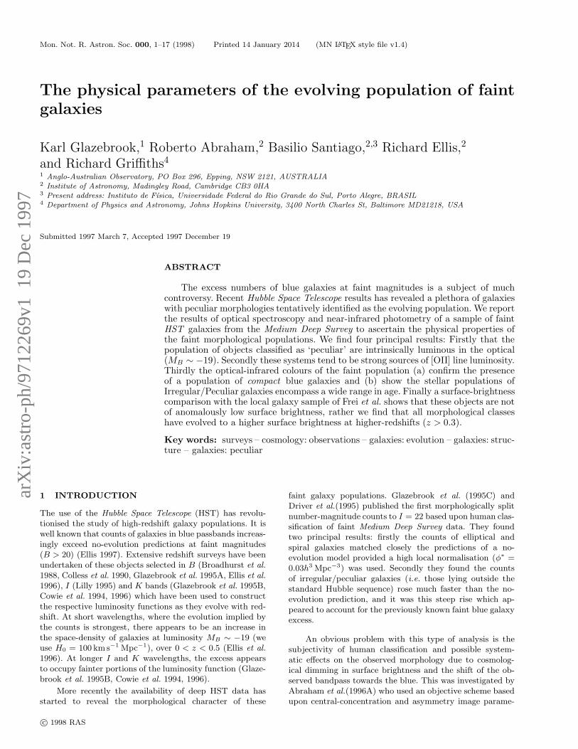
Figure 1. The morphological type vs I magnitude for the objectsin the photometric sample and the spectroscopic sample. Theclassifications are those of RSE from Abraham et al.(1996A) andthe key to the right shows the symbols used for these in laterfigures.

2.2 WHT spectroscopy

The spectroscopic observations were obtained using theLDSS2 multislit spectrograph during two runs: 4–6 Novem-ber, 1994 and 25–27 May, 1995. A total of 4 clear nights wereobtained. A full description of the LDSS2 spectrograph canbe found in Allington-Smith et al.(1994).

An LDSS2 mask was made for each of the MDS fieldsobserved. LDSS2 has a 10′ field for multislits, however sincethe HST MDS fields were only ∼ 3′ in size only ∼8–13slits could be put on target galaxies per mask. A total of 5masks were observed containing a total of 52 galaxies withan accumulated exposure time of 3-4 hours per mask. Theobservational procedure and data reduction were otherwiseidentical to that for the LDSS2 B < 24 redshift survey de-scribed in Glazebrook et al. 1995A. (I < 22 and B < 24are broadly equivalent in terms of typical S/N and meanredshift.)

The spectral identifications are given in Table 1. Theobject IDs are the same as given in Table 1 in the large cat-alog paper of Abraham et al.(1996A) which has been cross-referenced for magnitudes, colours, classifications and otherHST image parameters. We note that several of these fieldswere omitted from the original Abraham et al. paper due tothe galactic latitude cut to avoid crowded fields. The crowd-ing was subsequently found not to affect the A/C analysis orthe photometry. These A/C values have been redone and areincluded in Table 1, except in two cases where the imageswere too close to other bright objects for the A/C analysis.

The actual spectra are broadly similar to the range oftypes and S/N shown in Figure 1 of Glazebrook et al. andare not reproduced here. The use of the quality parameterQ for redshift identification confidence is the same as inGlazebrook et al.. and should have a similar reliability.

A total of 31 spectra were identified, one of which wasa star misclassified as an S0. The typical completeness ofeach mask was ∼ 50–70%, the overall completeness was 60%.While this was somewhat lower than the earlier LDSS2 sur-vey we believe that was due to insufficient S/N on the fainterobjects as most of the unidentified objects are concentratedin the range 21.5 < I < 22. If we just consider the brighter

c© 1998 RAS, MNRAS 000, 1–17

Physical parameters of faint galaxies 3

I < 21.5 sample the completeness is 78% out out of a totalsample of 27 objects. In the following discussion we iden-tify (by symbol size) the bright sample in the Figures andindicate the effect of identification completeness on our in-ferences. We believe our sample is robust enough for thescope of the analyses we will present below (primarily con-tinuum and line luminosities) since the number-redshift dis-tribution at I <

∼ 22 is already well established (Lilly et al.).The most important consideration is to ensure the identifica-tions cover the entire distribution of morphological types re-vealed by HST . This distribution is shown in Figure 1 whichdemonstrates that the identifications does indeed covers therange of types. They also cover the whole of the asymmetry-concentration diagram presented in Abraham et al. (1996A)as an alternative but equivalent measurement of the mor-phology. Thus we conclude our spectroscopic sample is is areasonable, albeit small, basis for looking at the physical pa-rameters as a function of morphology. The number-redshiftdistribution is discussed below in Section 3.

2.3 UKIRT photometry

The infrared observations for this project were collected ontwo observing runs: December 4–6 1994 and May 4–6 1995.The data was taken using the infrared camera IRCAM3which is a 256 × 256 indium antimonide (InSb) array. Aplate scale of 0.286′′ was used giving a field of view of 73′′

which is approximately the same as one HST chip in thegroup of three in the Wide Field Camera images.

In each field we observed 1–3 HST chips, choosing thechips and the exact centers in order to maximise the numberof I < 22 galaxy targets.

As the night sky varies considerably on the time-scale of15–30 minutes in the K-band we made individual exposuresof 2 minutes (each consisting of 12 frames of 10 secondsexposure averaged together), making inter-field offsets andreconstructing the sky flat-field by median filtering in groupsof 8. For the December run we offset the telescope betweenthe HST chips modulo a ±30 pixel dither pattern to attemptto get the best possible flatfield. However this tended toupset the guiding as often the guide star would be offsetpast the field dichroic causing a shift of a few arcsecondsin its optical image. Because of this during the May run wesimply dithered at each HST chip position separately. Theguiding was greatly improved and no significant differencewas obtained in the quality of the flatfield.

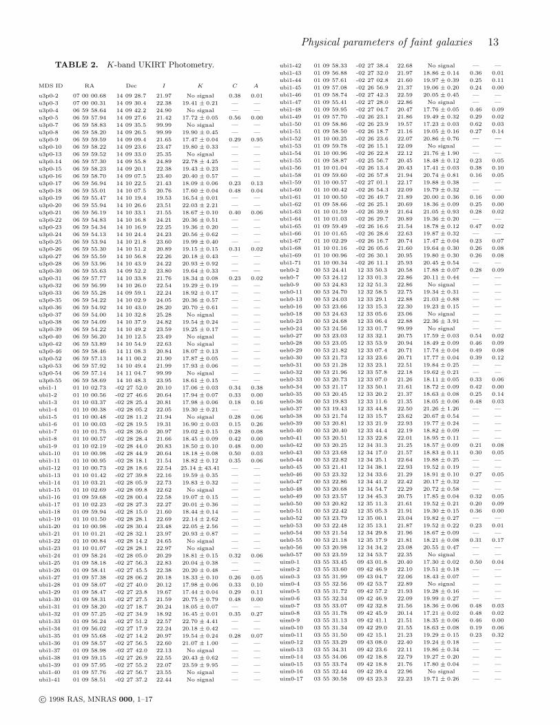
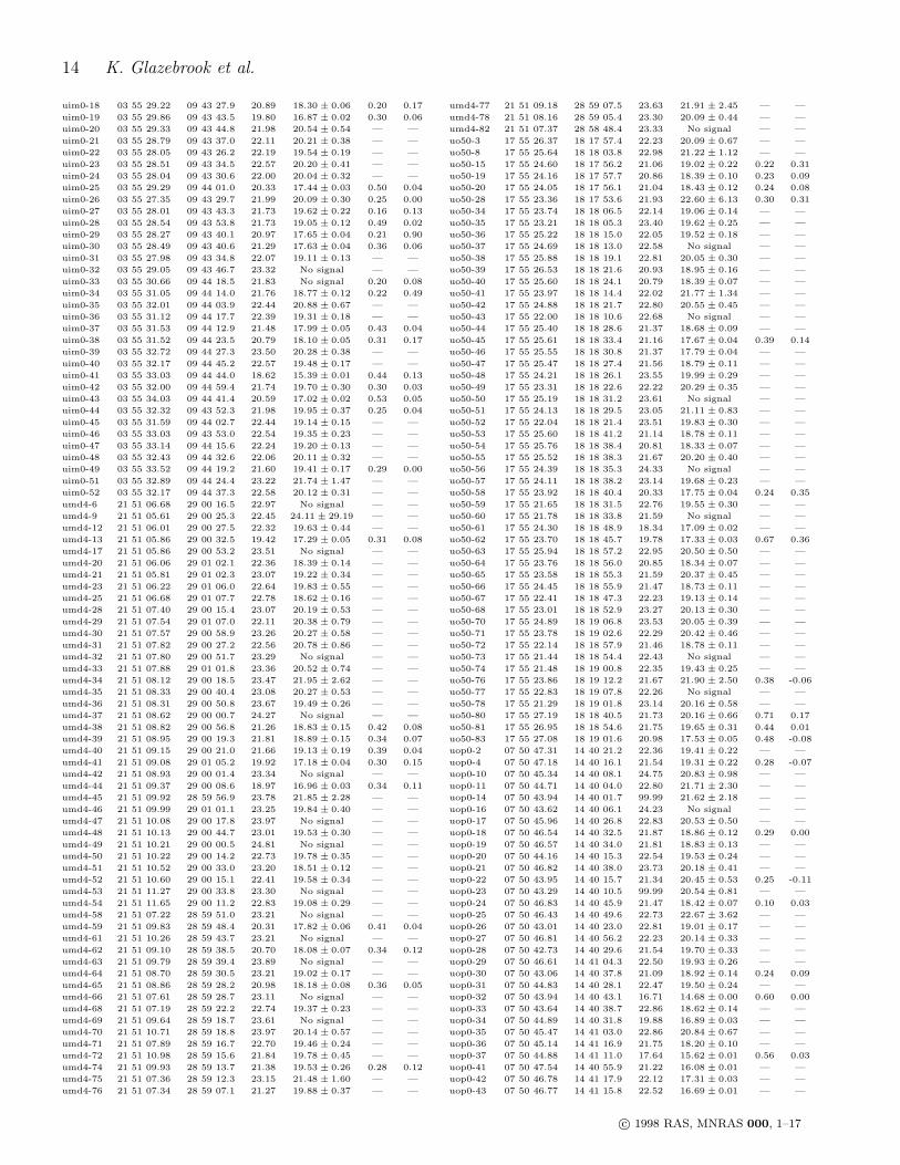
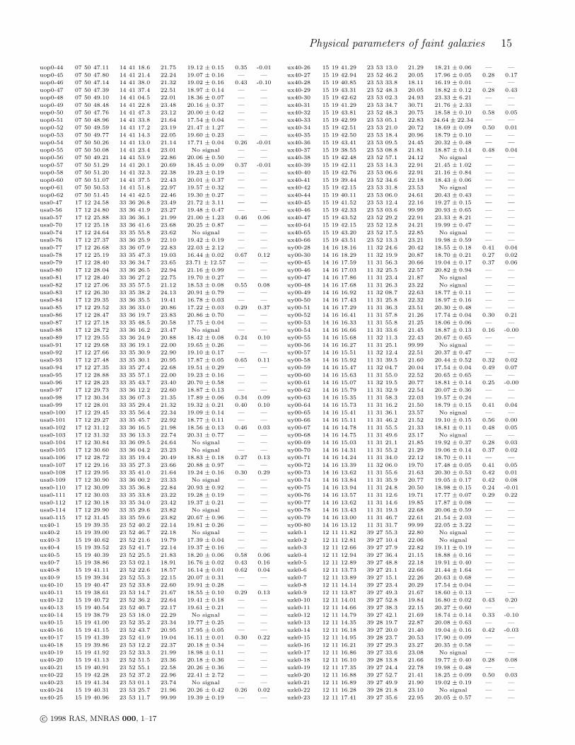
We had four clear nights in total over the two runs andobtained a K-band limit (3σ per pixel in a 2′′ diameter aper-ture) of K ≃ 21.5 in 11 HST fields covering 21 HST chippositions. with total on-target exposure times ranging from3000 s (in good conditions) to 10 000 s (in conditions of mod-erate extinction). At this limit we detected virtually all ofour I < 22 targets in this field. To obtain close to total K-magnitudes we used a 6′′ diameter aperture (matching ourcorrected HST apertures). In the sample 172 of the 218 ob-served galaxies had photometry δmK < 0.2 mags (roughlyequivalent to 5σ detections) and 202 of the 218 observedgalaxies had photometry δmK < 0.5 mags (roughly equiva-lent to 2σ detections), the rest being too faint in K. We usethe latter as our cutoff for our I − K photometry — sincewe doing photometry at sky positions determined from ourI-band images object detection is not an issue and so we can

go deeper into the noise. These K-magnitudes are given inTable 2 along with coordinates and A/C values from Abra-ham et al.. Note the A/C values of Abraham et al. have onlybe tabulated for I < 22, where their analysis stops. Addi-tionally a few extra objects with I < 22 were also omittedfrom the A/C analysis because the authors quite conserva-tive in rejecting objects too close to the field edge, too closeto other objects or contaminated by weak cosmic ray eventsor diffraction spikes.

3 THE LUMINOSITY OF FAINT GALAXIES

It has often been argued that the faint blue galaxy popu-lation could be a result of underestimating the number oflocal low surface-brightness or low-luminosity galaxies (e.g.McGaugh et al. 1994). These are then uncovered by the deepimaging surveys which have a lower surface brightness limit.However since the excess population has a similar n(z) tothe no-evolution prediction (Glazebrook et al. 1995A) it canbe inferred statistically that this is probably not the case:since the peak in n(z) occurs for L∗ galaxies (where L∗ isthe characteristic Schechter luminosity in the no-evolutionprediction) then the typical luminosity of the excess popu-lation must be ∼ L∗. This has been confirmed recently byluminosity function analyses of much larger samples (Elliset al. 1996) which show an increase in space density over0 < z < 0.5 at MB ≃ −19 (for H0 = 100 km s−1 Mpc−1).

With the sample we present here we are able to look atthe luminosities of individual galaxies directly, in order tosee how it depends on morphology.

3.1 B-band Absolute Magnitudes

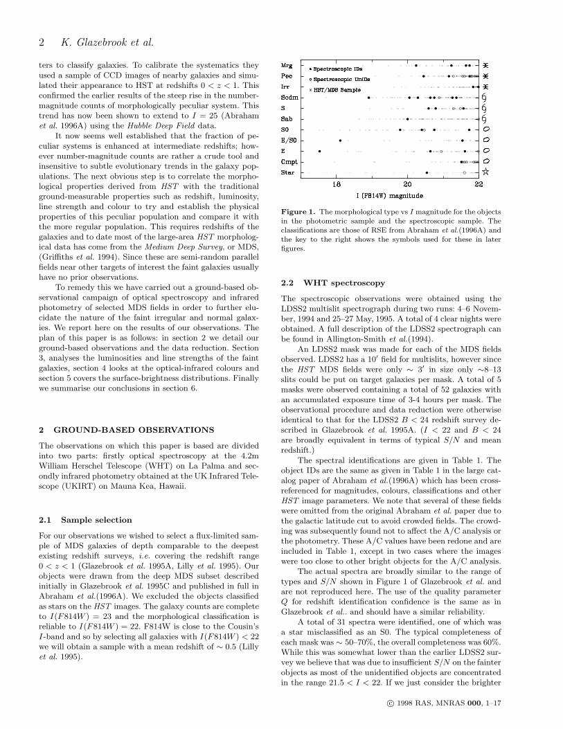
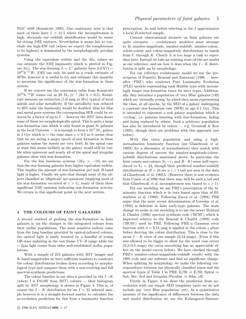
Since the observed I-band at z ∼ 0.8 is close to the rest-frame B-band, the K-correction is close to constant for allredshifts. This is shown in Figure 2(a) which shows the n(z)distribution of our sample overlayed with the I(observed)to B(rest) and B(observed) to B(rest) K-corrections usingour spectral energy distribution (SED) templates of localHubble types (those of Kennicutt 1992). The magnitude-redshift distributions of our morphological types is shown inFigure 2(b).

It can be seen that at the median redshift of our sample(z = 0.43) the range of K-correction over the SEDs is onlyhalf that it is in the B band. For z < 0.8 the I-band corre-sponds to rest frame V through R so there is no dependencyon the uncertain near-UV continua of nearby galaxies andour correction gets better at the higher redshifts. Finally aswe can assign physical morphological types from our HST

images we can assign an appropriate K-correction from thecorresponding spectral type. Even a gross error on the scaleof several spectral types (e.g. elliptical/spiral or spiral/Irr)would correspond to an error in MB of only 0.2 mags. Thuswe believe our K-corrections are much more robust than isusually the case and we can expect or MB values to be lim-ited by the accuracy of the photometry of the original HSTdata.

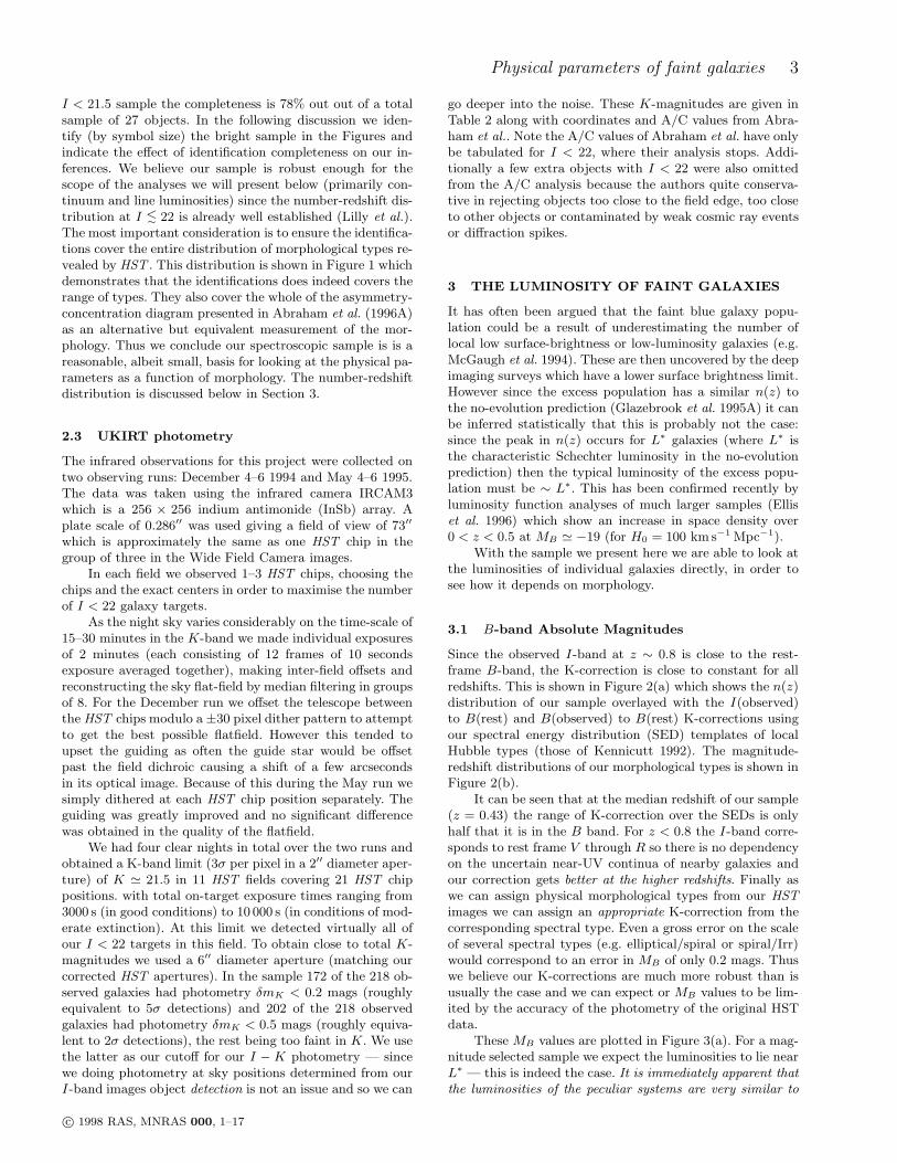
These MB values are plotted in Figure 3(a). For a mag-nitude selected sample we expect the luminosities to lie nearL∗ — this is indeed the case. It is immediately apparent that

the luminosities of the peculiar systems are very similar to

c© 1998 RAS, MNRAS 000, 1–17

4 K. Glazebrook et al.

Sab

Sbc

Scd

Sdm

Sdm

E/S0

E/S0

Figure 2. (a) The redshift distribution n(z) of our data togetherwith the K-corrections (I(observed) to B(rest) and B(observed)to B(rest)) for our E–Irr SEDs. (b) The redshift distribution bro-ken down by morphological type.

those of the elliptical and spiral galaxies. While some may bedwarfs (all of which are the fainter I > 21.5 objects) manyhave luminosities as bright at MB = −19. Thus we confirmdirectly what previously could only be inferred statistically.This implies that any model which tried to explain the ex-cess population via local dwarfs must include some degree of

luminosity evolution.

3.2 [OII] luminosity

Since we have spectra we can also look at the line emis-sion of these objects. We consider the faint-end slice with20 < I < 22 hereafter to exclude the brightest, low-redshiftobjects. Our spectra were unfluxed but we can directly mea-sure equivalent widths, this is shown in Figure 3(b). All ofthe objects had spectral windows including the [OII]-linelocation, the strength of this line is an indicator of star-formation. (Kennicutt 1992).

Figure 3. B-band continuum and [OII] emission line luminosi-ties. The bright objects (I < 21.5) are plotted with the largesymbols. (a) B luminosity and I (F814W) magnitude. (b) [OII]equivalent widths derived from the WHT spectra vs B luminos-ity (20 < I < 22), objects with no measurable [OII] (Wλ < 2–4A) are plotted at Wλ = 0). (c) Derived [OII] vs B luminosity(20 < I < 22). Objects with no measurable [OII] are plottedbelow the dashed line.

The previous deep redshift surveys (Broadhurst et al.

1988, Colless et al. 1990, Glazebrook et al. 1995A) estab-lished that the [OII] equivalent width distribution showed ahigh-end tail, not seen in local samples (Kennicutt 1992). Itcan be seen from Figure 3(b) most of the peculiar galaxieshave much higher equivalent widths than the other galaxies,in a region comparable to local starburst galaxies such as

c© 1998 RAS, MNRAS 000, 1–17

Physical parameters of faint galaxies 5

NGC 4449 (Kennicutt 1992). One cautionary note is thatmost of these have I > 21.5 where the incompleteness ishigh, obviously our redshift identification would be easierfor strong [OII] emitters. Nevertheless it seems fair to con-clude the high-EW tail (where we expect the completenessto be highest) is dominated by the morphologically peculiarsystems.

Using the equivalent widths and the MB values wecan estimate the [OII] luminosity which is plotted in Fig-ure 3(c). The star-forming L ∼ L∗ galaxies have L(OII) ∼

1034h−2 W. [OII] can only be used as a crude estimate ofSFRs, however it is useful to try and estimate this quantityto ascertain the significance of the star-formation in thesesystem.

If we convert use the conversion value from Kennicutt1034h−2 W comes out as 20 M⊙ yr−1 (for h = 0.5). Kenni-cutt assumes an extinction (1.0 mag at Hα) typical of localspirals and solar metallicity. If the metallicity was reducedto 20% solar the luminosity would be doubled, thus for blueand metal-poor systems the corresponding SFR could be re-duced by a factor of up to 5 — however the HST data showssome of them are morphologically spiral. This is quite a largestar-formation rate which is only found in giant Sc galaxiesin the local Universe — it is enough to form a 1011M⊙ galaxyin 5 Gyr which is ∼ the time since z = 0.5 so it seems clearthat we are seeing a major epoch of star formation in thesegalaxies unless the bursts are very brief. In the spiral caseat least this seems unlikely as the galaxy would still be visi-ble when quiescent and nearly all of the spiral and irregulargalaxies show this star-formation.

For the less luminous systems (MB > −18) we seethat the star-forming galaxies have higher equivalent widths.This implies the amount of star-formation per unit B-bandlight is higher. Finally we note that though most of the ob-jects classified as ‘ellipticals’ are quiescent (implying most ofthe star-formation occurred at z > 1), many of them showsignificant [OII] emission indicating star-formation activity.We return to this significant point in the next section.

4 THE COLOURS OF FAINT GALAXIES

A second method of probing the star-formation in faintgalaxies is via the changes in the integrated colours fromtheir stellar populations. The most sensitive indices comefrom the long baseline provided by optical-infrared colours;the optical light is easily boosted by a handful of youngOB stars radiating in the rest frame UV–B range while the∼ 2µm light comes from older well-established stellar popu-lations.

With a sample of 218 galaxies with HST images andK-band magnitudes we have sufficient numbers to constructthe colour distributions broken down according to morpho-logical type and compare them with a non-evolving and fullspectral-synthesis predictions.

The colour baseline in our data is provided by the I−K(where I is F814W from HST ) colours — their histogramsplit by HST morphology is shown in Figure 4. This is, ofcourse the I − K distribution for an I < 22 selected sam-ple however it is a straight-forward matter to calculate theno-evolution prediction for this from a luminosity function

prescription. As said before selecting in the I approximatesa local B-selected sample.

Current observational datasets on faint galaxies arequite extensive — evolutionary modelers must attemptto fit number-magnitude, number-redshift, number-colour,colour-colour and colour-magnitude distributions in bandsfrom U through K. Clearly it is too large a task to repro-duce here. Instead we take an existing state-of-the-art modelas our reference, and see how it does when the I −K distri-bution is split up by morphology.

For our reference evolutionary model we use the pre-scription of Pozzetti, Bruzual and Zamorani (1996 — here-after ‘PBZ’) who construct Pure Luminosity Evolution(PLE) models representing each Hubble type with increas-ingly longer star-formation times for later types. Addition-ally they introduce a population of ‘very Blue’ galaxies (vB)which are ‘eternally young’ by which they mean representingthe class, at all epochs, by the SED of a galaxy undergoinga constant star-formation rate (SFR) at age 0.1 Gyr. Thisis intended to represent a real galaxy population which is‘cycling’, i.e. galaxies bursting with star-formation, fadingand being replaced by others. Such a arbitrary populationhas also be introduced by others — e.g. Gronwall & Koo(1995), though there are problems with this approach (seebelow).

With this extra population and using a high-normalisation luminosity function (see Glazebrook et al.

1995C for a discussion of normalisation) they match withvarious degrees of success the number-magnitude-colour-redshift distributions mentioned above. In particular thefaint counts and colours (bj−rf and B−K) seem well repro-duced to bJ = 24, though their predicted number-redshiftdistributions at B = 24 see a z > 1 tail not seen in the dataof Glazebrook et al. 1995A. (However there is now evidencefrom Cowie et al.1996 that there may well be such a tail andthat Glazebrook et al. incompleteness was biased to z > 1).

For our modeling we use PBZ’s prescription of the lu-minosity function which is in turn based upon that of Ef-stathiou et al. (1988). Following Zucca et al. (1994) PBZargue that the more recent determination of Loveday et al.

(1992) is deficient in faint early-type galaxies. The mainchange we make in our modeling is to use the newer Bruzual& Charlot (1996) spectral synthesis code (‘BC95’) which isimproved relative to the Bruzual & Charlot (1993) code(‘BC93’) used by PBZ. Following PBZ a Gaussian errorfunction with σ = 0.15 mag is applied in the colour-z planebefore deriving the colour distribution. This is close to themean I − K error of our sample (0.14 mags). (Even if thiswas allowed to be bigger to allow for the worst case errors(0.2–0.3 mags) the extra smoothing has no appreciable ef-fect on the model curves below). We have checked throughPBZ’s number-colour-magnitude-redshift results with the1995 code and our software and find no significant change.When splitting by morphology we make the following cor-respondence between our physically classified types and thespectral types of Table 1 in PBZ: E/S0 ⇒ E/S0, Spiral ⇒Sab, Sbc, Scd and Irregular/Peculiar ⇒ Sdm, vB.

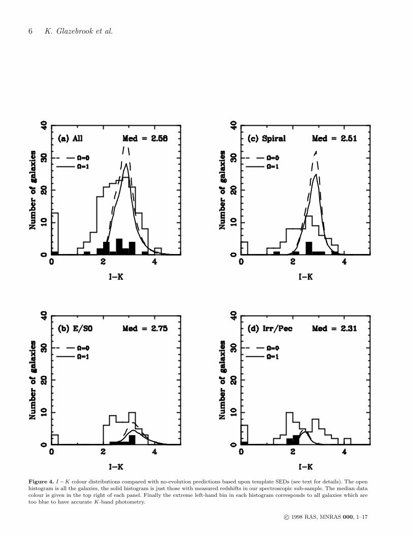
Firstly in Figure 4 we show the prediction from no-evolution with our simple SED templates (note we do notinclude any ‘very Blue population’ yet). As a quantitativemeasure of the significance of differences between the dataand model distribution we use the Kolmogorov-Smirnov

c© 1998 RAS, MNRAS 000, 1–17

6 K. Glazebrook et al.

Figure 4. I −K colour distributions compared with no-evolution predictions based upon template SEDs (see text for details). The openhistogram is all the galaxies, the solid histogram is just those with measured redshifts in our spectroscopic sub-sample. The median datacolour is given in the top right of each panel. Finally the extreme left-hand bin in each histogram corresponds to all galaxies which aretoo blue to have accurate K-band photometry.

c© 1998 RAS, MNRAS 000, 1–17

Physical parameters of faint galaxies 7

test, this is shown in Table 3. When the two differ withmore than 99% confidence log PKS < −2. (Note: to do thiswe need to ignore the K non-detections, i.e. the leftmostbins in the histogram figures. However these only represent7% of objects so we believe the following conclusions are ro-bust.) Table 3 also give the ‘excess’ parameter (XS) — i.e.

the ratio of the number of galaxies observed to the numberpredicted. Panel (a) of Figure 4 reproduces the known 50–100% (dependent on Ω) excess of faint galaxies at I = 22,and it can be seen that most of the excess population isindeed blue. Breaking down by morphology and inspectingthe figures and log PKS parameters it is clear that: (a) thereis a significant excess of blue ‘ellipticals’, (b) the spiral dis-tribution has a bluer median colour and (c) while many ofthe Irr/Pec galaxies are indeed very blue many of them havemore normal, older colours indicating that they do not rep-resent a simple ‘very blue’ population. We have also exam-ined the effect on the colour distribution of using the late-age PBZ models as no-evolution SEDs and find the ellipticalpredictions become ∼ 0.2 mag redder and the spiral+Irr pre-diction becomes ∼ 0.2 mag bluer. This reflects the accuracywith which the PBZ models match the data at late times.We have also carried out a study of the effects of metallicityusing an early version of the ‘BC96’ code (Bruzual & Char-lot in preparation). As expected this was small — varyingthe metallicity from solar to 20% of solar makes the I − Kcolours only 0.2–0.6 mag bluer over 0 < z < 1.

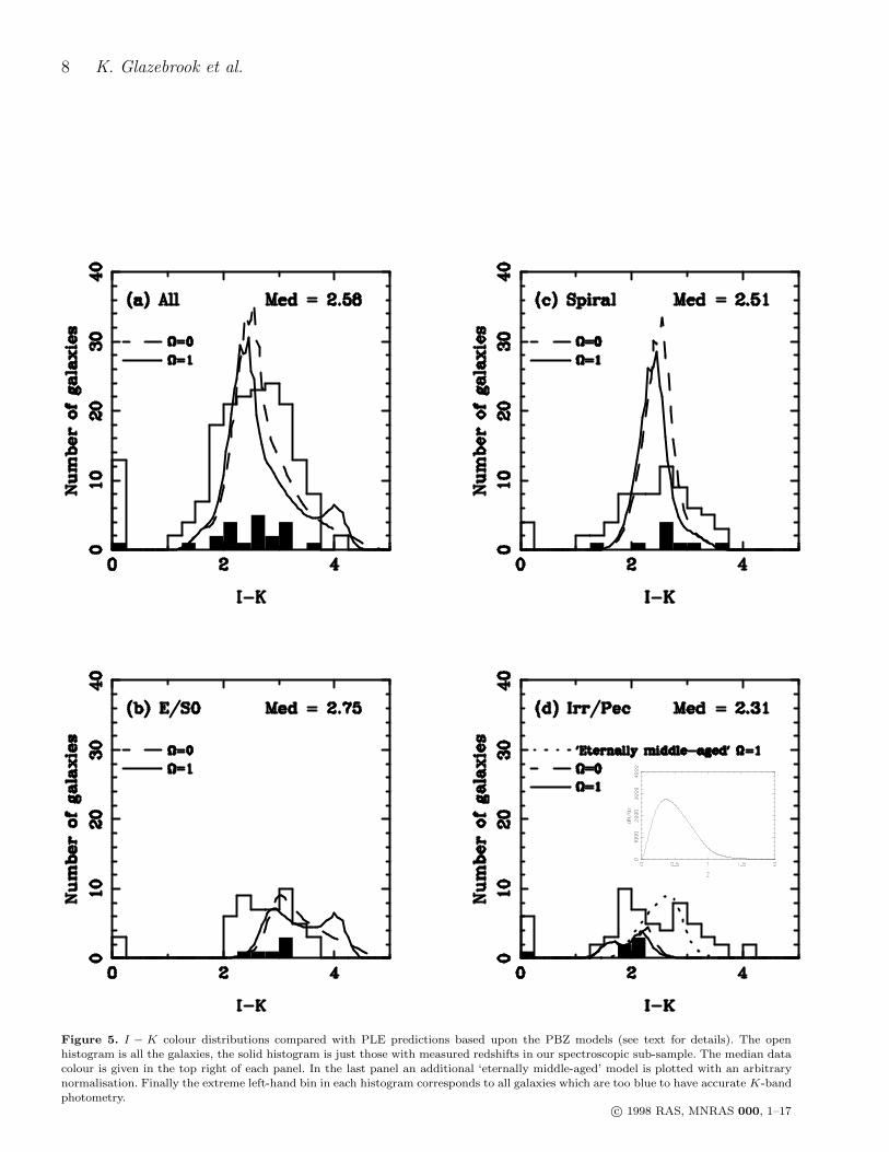
To investigate this in more detail we plot in Figure 5 thePBZ evolving models (now including the ‘eternally young’galaxies). Several points of interest are apparent:

(i) There is a broad agreement in the colour distributionand normalisation of all galaxies. There is still a ∼ 30–50%excess at I = 22 even with this model including extra ‘veryBlue’ galaxies. This is also seen in the number-magnitudecounts (Figure 3(d) of PBZ) when plotted on an expandedscale. In our data the significance of this excess is marginal,especially in light of the uncertainties surrounding the abso-lute normalisation of the local luminosity function. Howeverwhen we look at the breakdown by morphology a more com-plex picture emerges:

(ii) Even with evolution put in there is still an excess ofblue ‘ellipticals’. Note the evolution for ellipticals in the PBZmodels is close to ‘passive evolution’ but not quite becauseellipticals are slightly better represented by an exponentiallydecaying SFR with a short e-folding time rather than a sin-gle short burst (though after 5 Gyr there is little difference).Inspection of the images of the blue galaxies (defining themas I − K < 2.5) does indeed show them to be compactobjects, occasionally with a very weak disk. These objectsmake up 36% of the objects which are classified as ‘elliptical’by the compactness criteria in the HST images and 10% ofall galaxies — S0 galaxies should have similar colours to el-lipticals and even contamination by Sa galaxies would onlylead to colours ∼ 0.2 mag bluer. We provisionally identifythe blue compact galaxies as the same population as the‘Blue Nucleated Galaxies’ of Schade et al. (1995, 1996A)who find a similar proportion (14%). All of the [OII] emit-ting ‘ellipticals’ in Figure 3 (and one extra with I < 20)correspond to galaxies with I − K < 3.2 and the (strongestWλ[OII] = 42A) is the bluest (I = 18.1, I − K = 1.9). Wehypothesise these do not correspond to local ellipticals since

the latter are reasonably accounted for by the red end of thedistribution. Note that PBZ use a faint end slope for theirelliptical luminosity function of α = −0.48, if the slope isflattened to −1.00 as used in Glazebrook et al. (1995C) theprimary effect is to increase the normalisation of the modelcurves by ≃ 30% and bluen the median colours by 0.2 mag-nitude (due to the slightly lower mean redshift). This changedoes not affect these arguments.

(iii) The spiral I − K distribution agrees in mean colourand normalisation with the model predictions, shifting blue-wards by ∼ 0.3 magnitudes compared to the non-evolvingSED prediction. However this shift is smaller (0.1 mag) rel-ative to the non-evolving PBZ prediction so it is not clearhow significant this is. The blue tail of the distribution isnow better matched, though the range of colours in the datais still slightly broader than the model prediction. The dis-crepancy is quite significant. This implies to us that realspirals have a more complex distribution of star-formationhistories, or of metallicity or extinction, than in these simplesingle-history models.

(iv) The Irregular/Peculiar class are the most interestingin that the show a surprisingly broad distribution of I − Kcolours. In the models they are only represented by galaxieswhich are very blue. The model curves in Figure 5(d) showtwo blue peaks. The first peak at I − K = 2.2 is due tothe model Sdm galaxies and the second one at I − K = 1.6is due to the vB class. In contrast the data extends out togalaxies with I − K = 4. Visual inspection of all Irr/Pecgalaxies with I −K > 3 show that they do indeed belong inthis class. Examination of their position in the Asymmetry-Concentration diagram of Abraham et al. (1996A) showsthe red Irr/Pec galaxies are not very different from the blueIrr/Pec galaxies. There is also no large K-correction effectswhich may be making the colours redder — the inset toFigure 5(d) shows the model n(z) which is not too differentfrom our measured redshifts of these galaxies at this mag-nitude in Section 2. This may not be so convincing sincethe solid histogram in Figure 5 shows we only succeeded ingetting redshifts for the bluer galaxies. However the largeground-based Canada-France Redshift Survey (Lilly et al.

1995) was selected to I < 22 and of ∼ 500 galaxies themaximum redshift was only ∼ 1.3. Sdm galaxies can be asred as I − K = 3.5 for 1.3 < z < 2 but in this case theywould have to be 1–2 magnitudes more luminous. The ‘eter-nally young’ population is so blue it has I − K < 2 evenout to z = 4. We argue that the most likely explanation isthat a simple representation of this morphologically pecu-liar population as a population of ‘eternally young’ (or evenSdm type) star-forming galaxies is over-simplistic. The red-der galaxies can be better matched with an older population— this is demonstrated in Figure 5 by showing the predic-tion for an arbitrary ‘eternally middle-aged’ population ofage 5 Gyr post-starburst, which gives a much better matchto the spread of colours. While of course this is an merelyillustrative it is clear that the Irr/Pec population must bemade of galaxies with a spread of age (at least 0–5 Gyr)unless they were very unusual in metallicity or dust. In thelatter case to match the red end of the I − K histograman extinction of AI = 1.7 mags is required. However sincethe sample is selected in the I-band applying this amountof extinction to the galaxy luminosities reduces the I < 22space density by a factor of ∼ 10. Thus many more galax-

c© 1998 RAS, MNRAS 000, 1–17

8 K. Glazebrook et al.

Figure 5. I − K colour distributions compared with PLE predictions based upon the PBZ models (see text for details). The openhistogram is all the galaxies, the solid histogram is just those with measured redshifts in our spectroscopic sub-sample. The median datacolour is given in the top right of each panel. In the last panel an additional ‘eternally middle-aged’ model is plotted with an arbitrarynormalisation. Finally the extreme left-hand bin in each histogram corresponds to all galaxies which are too blue to have accurate K-bandphotometry.

c© 1998 RAS, MNRAS 000, 1–17

Physical parameters of faint galaxies 9

ies are required to match the counts. Of course this couldin principle by compensated for by making the underlyingluminosity of the dusty galaxies much greater. Finally wenote that between from 5 to 10 Gyr (∼ z = 0.5 to z = 0)a pure starburst would fade by < 0.2 mags in the UBVbands so should be seen in the local luminosity function inthe absence of other effects (a point explored in more detailby Bouwens & Silk, 1996).

5 THE SURFACE BRIGHTNESS OF FAINTGALAXIES

A counterpoint to the suggestions that the faint blue galaxypopulation may be low-luminosity has been the suggestionthat they may constitute a low surface brightness popula-tion. This is a natural hypothesis because the deep CCD sur-veys which uncover the faint blue galaxies also go to fainterlimiting surface brightnesses (McGaugh et al. 1994). How-ever it is difficult to test due to isophotal effects. In a givensurvey while surface brightness may be subject to (1 + z)4

dimming with redshift (plus K-corrections) this will alsocause the area of a galaxy above a fixed observed isophote toshrink. Thus only the inner parts of the galaxy are sampledwhich can lead to an increase in isophotal surface brightness.

One approach, as adopted by Schade et al. (1995,1996A, 1996B) is to try and fit theoretical profile modelsto the galaxy images — once the central surface brightnessand scale length is fitted a total magnitude for the modelcan be calculated. Of course this requires that the galaxyprofile follows a simple form.

In our analysis of the MDS data we adopt an orthogo-nal approach based on the work of Abraham et al. (1996A)— we compute a simple parameter (the isophotal surfacebrightness) and compare against artificially-redshifted lo-cal galaxy templates using the same parameter to allow forthe aforementioned selection effects. The sample we use isthat of Frei et al. (1996), who chose galaxies which werebright, well-resolved and covered a wide range of morpho-logical classes. The luminosities range from MB = −21to MB = −15, peaking around M∗, thus approximatingquite well the range of luminosities seen in faint magnitude-selected samples (Brinchmann et al., 1997).

In the artificial redshifting procedure a spectral energydistribution is assigned to each part of the galaxy, it’s imagein the F814W filter at the appropriate redshift is computedand the image is binned up and noise is added so it is simu-lated as observed with HST. Optionally we scale the galaxyflux to crudely allow for a simple linear brightness evolu-tion (∆M = −2z). Finally we measure the mean surfacebrightness above a fixed isophote of I = 24.0 mags/arcsec−2

which is approximately twice the typical noise level in theMDS data. This allows us to make a differential compar-ison between the MDS galaxies and the local galaxies asthey would be viewed by HST at the same redshift with aminimum of modeling uncertainty.

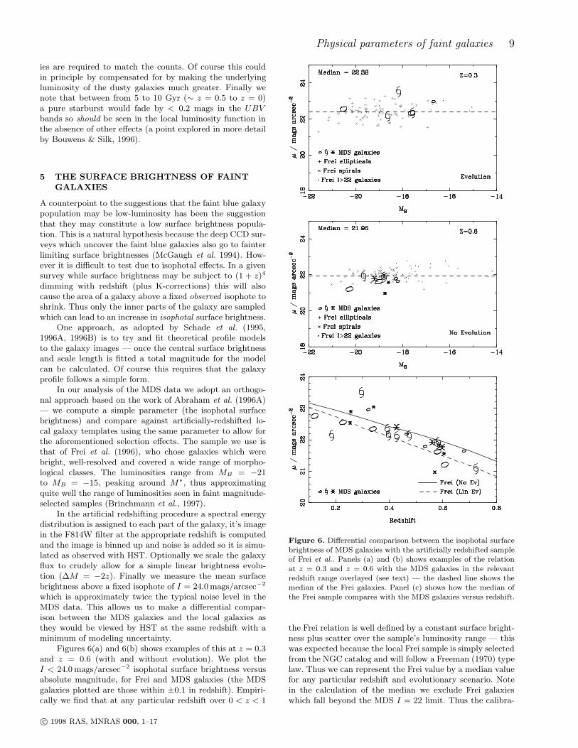
Figures 6(a) and 6(b) shows examples of this at z = 0.3and z = 0.6 (with and without evolution). We plot theI < 24.0 mags/arcsec−2 isophotal surface brightness versusabsolute magnitude, for Frei and MDS galaxies (the MDSgalaxies plotted are those within ±0.1 in redshift). Empiri-cally we find that at any particular redshift over 0 < z < 1

Figure 6. Differential comparison between the isophotal surfacebrightness of MDS galaxies with the artificially redshifted sampleof Frei et al.. Panels (a) and (b) shows examples of the relationat z = 0.3 and z = 0.6 with the MDS galaxies in the relevantredshift range overlayed (see text) — the dashed line shows themedian of the Frei galaxies. Panel (c) shows how the median ofthe Frei sample compares with the MDS galaxies versus redshift.

the Frei relation is well defined by a constant surface bright-ness plus scatter over the sample’s luminosity range — thiswas expected because the local Frei sample is simply selectedfrom the NGC catalog and will follow a Freeman (1970) typelaw. Thus we can represent the Frei value by a median valuefor any particular redshift and evolutionary scenario. Notein the calculation of the median we exclude Frei galaxieswhich fall beyond the MDS I = 22 limit. Thus the calibra-

c© 1998 RAS, MNRAS 000, 1–17

10 K. Glazebrook et al.

tion sample exhibits the same bias to more luminous galax-ies at higher redshifts as the MDS. In practice however wefound this exclusion makes no difference to the final resultas the I > 22 galaxies have similar surface brightnesses (ascan be seen in Figures 6(a) and (b)).

This leads us to Figure 6(c) which plots the median ofthe Frei sample against redshift (both with and without evo-lution) and compares with the MDS galaxies. It can be seenthat the MDS galaxies are consistently brighter than theirlocal counterparts for z > 0.3. Comparing with the arbi-trarily evolved local counterparts (whose evolution amountsto 2 magnitudes at z = 1) we estimate that typically theamount of evolution in the MDS galaxies is about half this— i.e. about 1 magnitude by z = 1. This can also be seendirectly in the z = 0.6 redshift slice shown in Figure 6(b).This conclusion still holds when considering the I < 21.5high-completeness sub-sample and we conclude we are see-ing a genuine evolutionary effect providing the Frei sample

is representative of local galaxies.The amount of this brightening is the same as found by

Schade et al. from their fitting method, like Schade et al. wealso find the brightening appears to apply to objects of allmorphologies.

6 CONCLUSIONS

We conclude:

(i) The faint-blue galaxy excess to I = 22 is not due tonearby under-luminous galaxies being revealed by faint sur-veys, rather that many of the objects are observed to beclose to L∗. This is true for all morphological classes. Thus,for example, we can not simply explain the excess of pe-culiar systems by a uniform population of low-luminositydwarf galaxies being revealed by deep surveys.

(ii) A significant component of the blue excess (∼ 10%)is composed of compact blue objects originally classified as‘ellipticals’. These are provisionally identified with the ‘BlueNucleated Galaxies’ of Schade et al. (1995, 1996).

(iii) The red envelope of the population of compact ob-jects at z ∼ 0.5 accounts for the number of elliptical galaxieswe see today.

(iv) We see tentative evidence for some mild colour evolu-tion in the population of spiral galaxies though it is not clearhow significant this is given the uncertainty in the models,and overall broader range of colours than exhibited by themodels.

(v) The galaxies in the Irr/Peculiar morphological classcan not simply be represented by a simple population of veryyoung blue galaxies. Rather the broad distribution of blueand red colours indicate a range of ages (0–5 Gyr), if in-terpreted as stellar populations, or luminous dusty galaxieswith extinctions of up to 3 mags in the I-band. We concludethat models such as those of Pozzetti et al. or Gronwall &Koo (1995) are too simplistic. This adds to the other knownproblem with these types of model — the predicted over-abundance of low-luminosity galaxies at z = 0 (Bouwens &Silk, 1996). The properties and evolution of the very late-type galaxies is clearly not well understood yet.

(vi) The line-luminosities in [OII] indicate significantamounts of star-formation is occurring at z = 0.5, primarily

in the late-type Irr/Pec population but also in the spiralsand blue ‘ellipticals’.

(vii) The surface brightness relation shows no evidencethat any of the faint morphological populations are ofanomalously low surface brightness. Rather we confirm theresult of Schade et al. (1995, 1996A, 1996B), from a com-pletely different non-parametric method (comparison withthe artificially-redshifted Frei et al. local sample), of ev-idence for about 1 magnitude evolution towards a highersurface brightness, in all morphological classes, for z > 0.3.

(viii) There is a lack of success in measuring the redshiftsfor the redder peculiar systems, so it is difficult to constrainthem in any way. It is entirely possible they may be anoma-lous in luminosity, redshift or surface brightness. Howeverit is clear that the peculiar population is not homogeneousand this must be accounted for in any realistic evolution-ary model. A spectroscopic campaign targeted at these redobjects would of immense value in understanding the popu-lation of peculiar objects revealed in faint HST images.

It is obvious that larger samples with spectroscopy andHST imaging are desirable to further this work; with theadvent of large HST imaging programmes in Cycles 6 and7 samples of several hundred objects are becoming available(e.g. Brinchmann et al.. 1997). Also the spectral synthesismodels are being improved (e.g. the ‘BC96’ Bruzual andCharlot code, in preparation) and it will be possible to in-clude in the models effects such as varying metallicity. Withvery deep multi-colour HST images there is also the pos-sibility of looking at the star-formation history of differentportions of an individual galaxy (Abraham et al.. 1997). Itis clear that in the next few years a much more detailedunderstanding of the evolution and properties of the faintgalaxy populations will be achieved.

7 ACKNOWLEDGEMENTS

The authors thank Stefan Charlot for his generosity inmaking his 1995 spectral synthesis code available to us.This paper is based on observations with the NASA/ESAHubble Space Telescope, obtained at the Space TelescopeScience Institute, which is operated by the Association ofUniversities for Research in Astronomy Inc., under NASAcontract NAS5-26555. Coordination and analysis of datafrom the Medium Deep Survey is funded by STScI grantsGO2684.0X.87A and GO3917.OX.91A. We also gratefullyacknowledge the generous allocations of telescope time onthe UK Infrared Telescope, operated by the Royal Obser-vatory Edinburgh and the William Herschel Telescope, op-erated by the Royal Greenwich Observatory in the SpanishObservatorio del Roque de Los Muchachos of the Institutode Astrofısica de Canarias. We also thank the staff and tele-scope operators of these telescopes for their enthusiasm andcompetent support. The data reduction and analysis wasperformed primarily with computer hardware supplied bySTARLINK. All the authors acknowledge funding for thisresearch from the PPARC.

REFERENCES

c© 1998 RAS, MNRAS 000, 1–17

Physical parameters of faint galaxies 11

Abraham R. G., van den Bergh, S., Glazebrook K., Ellis R. S.,

Santiago B. X., Surma P., Griffiths R. E., 1996A, ApJS, 107,1

Abraham R. G., Tanvir N. R., Santiago B. X., Ellis R. S., Glaze-brook K., van den Bergh S., 1996B, MNRAS, 279, L47

Abraham R. G., et al., 1997, in preparationAllington-Smith J. R., Breare J. M., Ellis R. S., Gellatly D. W.,

Glazebrook K., Jorden P. R., MacLean J. F., Oates A. P.,et al.., 1994, PASP, 106, 983

Bouwens R. J., Silk J., 1996, ApJ, 471, L19Brinchmann J., et al., 1997, in preparationBroadhurst T. J., Ellis R. S., Shanks T., 1988, MNRAS, 235, 827Bruzual G., Charlot S., 1993, ApJ, 405, 538Bruzual G., Charlot S., 1996, ApJ, in pressColless M. M., Ellis R. S., Taylor K., Shaw G., 1991, MNRAS,

253, 686Cowie L. L, Gardner J. P., Hu E. M., Songalia A., Hodapp K.

W., Wainscoat R. J., 1994, ApJS, 94, 461Cowie L. L., Songalia A., Hu E. M., 1996. ApJ, in pressDriver S. P., Windhorst R. A., Griffiths R. E., 1995, ApJ, 453, 48Efstathiou G., Ellis R. S., Peterson B. A., 1988, MNRAS 232, 431Ellis R. S., 1997, Annu. Rev. Astron. Astrophys., 35.Ellis R. S., Colless M. M., Broadhurst T. J., Heyl J., Glazebrook

K., 1996, MNRAS, 280, 235Freeman K., 1970, ApJ, 160, 811Frei Z., Guhathakurta P., Gunn J. E., 1996, Astron. J., 111, 174Glazebrook K., Ellis R. S., Colless M. M, Broadhurst T. J.,

Allington-Smith J. R., Tanvir N. R., 1995A, MNRAS, 273,157

Glazebrook K., Peacock J. A., Miller L., Collins C. A., 1995B,MNRAS, 275, 169

Glazebrook K., Ellis R. S., Santiago B. X., Griffiths R. E., 1995C,MNRAS, 275, L19

Griffiths R. E., Casertano S., Ratnatunga K. U., Neuschaefer L.W., Ellis R. S., Gilmore G. F., Glazebrook K., Santiago B.,Huchra J. P., Windhorst R. A., et al., 1994, ApJ, 435, L19

Gronwall C., Koo D. C., 1995, ApJ, 440, L1Kennicutt R. C., 1992, ApJ, 388, 310Lilly S. J., Le Fevre O., Crampton. D., Hammer F.,Tresse L.,

1995, ApJ, 455, 50Loveday J., Peterson B. A., Efstathiou G., Maddox S. J., 1992.

ApJ, 390, 338McGaugh S. S., 1994, Nat, 367, 538Schade D. J., Lilly S. J., Hammer F., Le Fevre O., Crampton D.,

Tresse L., 1995, ApJ 455, L1Schade D. J., Lilly S. J., Crampton D., Hammer F., Le Fevre O.,

1996A, ApJ in press

Schade D. J., Carlberg R. G., Yee H. K. C., Lopez-Cruz, 1996B,ApJ 464, L63.

Pozzetti L., Bruzual G., Zamorani G., 1996, MNRAS, 281, 953(PBZ)

Wynn C. G., Worswick S. P., 1988, Observatory, 108, 161Zucca E., Pozzetti L., Zamorani G., 1994, MNRAS 269, 953

c© 1998 RAS, MNRAS 000, 1–17

12 K. Glazebrook et al.

8 TABLES

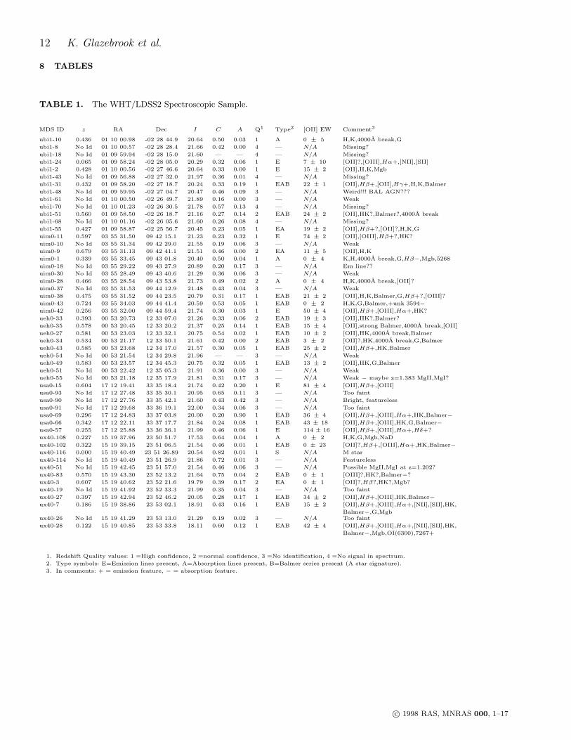
TABLE 1. The WHT/LDSS2 Spectroscopic Sample.

MDS ID z RA Dec I C A Q1 Type2 [OII] EW Comment3

ubi1-10 0.436 01 10 00.98 -02 28 44.9 20.64 0.50 0.03 1 A 0 ± 5 H,K,4000A break,G

ubi1-8 No Id 01 10 00.57 -02 28 28.4 21.66 0.42 0.00 4 — N/A Missing?

ubi1-18 No Id 01 09 59.94 -02 28 15.0 21.60 — — 4 — N/A Missing?

ubi1-24 0.065 01 09 58.24 -02 28 05.0 20.29 0.32 0.06 1 E 7 ± 10 [OII]?,[OIII],Hα+,[NII],[SII]

ubi1-2 0.428 01 10 00.56 -02 27 46.6 20.64 0.33 0.00 1 E 15 ± 2 [OII],H,K,Mgb

ubi1-43 No Id 01 09 56.88 -02 27 32.0 21.97 0.36 0.01 4 — N/A Missing?

ubi1-31 0.432 01 09 58.20 -02 27 18.7 20.24 0.33 0.19 1 EAB 22 ± 1 [OII],Hβ+,[OII],Hγ+,H,K,Balmer

ubi1-48 No Id 01 09 59.95 -02 27 04.7 20.47 0.46 0.09 3 — N/A Weird!!! BAL AGN???

ubi1-61 No Id 01 10 00.50 -02 26 49.7 21.89 0.16 0.00 3 — N/A Weak

ubi1-70 No Id 01 10 01.23 -02 26 30.5 21.78 0.57 0.13 4 — N/A Missing?

ubi1-51 0.560 01 09 58.50 -02 26 18.7 21.16 0.27 0.14 2 EAB 24 ± 2 [OII],HK?,Balmer?,4000A break

ubi1-68 No Id 01 10 01.16 -02 26 05.6 21.60 0.26 0.08 4 — N/A Missing?

ubi1-55 0.427 01 09 58.87 -02 25 56.7 20.45 0.23 0.05 1 EA 19 ± 2 [OII],Hβ+?,[OII]?,H,K,G

uim0-11 0.597 03 55 31.50 09 42 15.1 21.23 0.23 0.32 1 E 74 ± 2 [OII],[OIII],Hβ+?,HK?

uim0-10 No Id 03 55 31.34 09 42 29.0 21.55 0.19 0.06 3 — N/A Weak

uim0-9 0.679 03 55 31.13 09 42 41.1 21.51 0.46 0.00 2 EA 11 ± 5 [OII],H,K

uim0-1 0.339 03 55 33.45 09 43 01.8 20.40 0.50 0.04 1 A 0 ± 4 K,H,4000A break,G,Hβ−,Mgb,5268

uim0-18 No Id 03 55 29.22 09 43 27.9 20.89 0.20 0.17 3 — N/A Em line??

uim0-30 No Id 03 55 28.49 09 43 40.6 21.29 0.36 0.06 3 — N/A Weak

uim0-28 0.466 03 55 28.54 09 43 53.8 21.73 0.49 0.02 2 A 0 ± 4 H,K,4000A break,[OII]?

uim0-37 No Id 03 55 31.53 09 44 12.9 21.48 0.43 0.04 3 — N/A Weak

uim0-38 0.475 03 55 31.52 09 44 23.5 20.79 0.31 0.17 1 EAB 21 ± 2 [OII],H,K,Balmer,G,Hβ+?,[OIII]?

uim0-43 0.724 03 55 34.03 09 44 41.4 20.59 0.53 0.05 1 EAB 0 ± 2 H,K,G,Balmer,+unk 3594−

uim0-42 0.256 03 55 32.00 09 44 59.4 21.74 0.30 0.03 1 E 50 ± 4 [OII],Hβ+,[OIII],Hα+,HK?

ueh0-33 0.393 00 53 20.73 12 33 07.0 21.26 0.33 0.06 2 EAB 19 ± 3 [OII],HK?,Balmer?

ueh0-35 0.578 00 53 20.45 12 33 20.2 21.37 0.25 0.14 1 EAB 15 ± 4 [OII],strong Balmer,4000A break,[OII]

ueh0-27 0.581 00 53 23.03 12 33 32.1 20.75 0.54 0.02 1 EAB 10 ± 2 [OII],HK,4000A break,Balmer

ueh0-34 0.534 00 53 21.17 12 33 50.1 21.61 0.42 0.00 2 EAB 3 ± 2 [OII]?,HK,4000A break,G,Balmer

ueh0-43 0.585 00 53 23.68 12 34 17.0 21.57 0.30 0.05 1 EAB 25 ± 2 [OII],Hβ+,HK,Balmer

ueh0-54 No Id 00 53 21.54 12 34 29.8 21.96 — — 3 — N/A Weak

ueh0-49 0.583 00 53 23.57 12 34 45.3 20.75 0.32 0.05 1 EAB 13 ± 2 [OII],HK,G,Balmer

ueh0-51 No Id 00 53 22.42 12 35 05.3 21.91 0.36 0.00 3 — N/A Weak

ueh0-55 No Id 00 53 21.18 12 35 17.9 21.81 0.31 0.17 3 — N/A Weak − maybe z=1.383 MgII,MgI?

usa0-15 0.604 17 12 19.41 33 35 18.4 21.74 0.42 0.20 1 E 81 ± 4 [OII],Hβ+,[OIII]

usa0-93 No Id 17 12 27.48 33 35 30.1 20.95 0.65 0.11 3 — N/A Too faint

usa0-90 No Id 17 12 27.76 33 35 42.1 21.60 0.43 0.42 3 — N/A Bright, featureless

usa0-91 No Id 17 12 29.68 33 36 19.1 22.00 0.34 0.06 3 — N/A Too faint

usa0-69 0.296 17 12 24.83 33 37 03.8 20.00 0.20 0.90 1 EAB 36 ± 4 [OII],Hβ+,[OIII],Hα+,HK,Balmer−

usa0-66 0.342 17 12 22.11 33 37 17.7 21.84 0.24 0.08 1 EAB 43 ± 18 [OII],Hβ+,[OIII],HK,G,Balmer−

usa0-57 0.255 17 12 25.88 33 36 36.1 21.99 0.46 0.06 1 E 114 ± 16 [OII],Hβ+,[OIII],Hα+,Hδ+?

ux40-108 0.227 15 19 37.96 23 50 51.7 17.53 0.64 0.04 1 A 0 ± 2 H,K,G,Mgb,NaD

ux40-102 0.322 15 19 39.15 23 51 06.5 21.54 0.46 0.01 1 EAB 0 ± 23 [OII]?,Hβ+,[OIII],Hα+,HK,Balmer−

ux40-116 0.000 15 19 40.49 23 51 26.89 20.54 0.82 0.01 1 S N/A M star

ux40-114 No Id 15 19 40.49 23 51 26.9 21.86 0.72 0.01 3 — N/A Featureless

ux40-51 No Id 15 19 42.45 23 51 57.0 21.54 0.46 0.06 3 — N/A Possible MgII,MgI at z=1.202?

ux40-83 0.570 15 19 43.30 23 52 13.2 21.64 0.75 0.04 2 EAB 0 ± 1 [OIII]?,HK?,Balmer−?

ux40-3 0.607 15 19 40.62 23 52 21.6 19.79 0.39 0.17 2 EA 0 ± 1 [OII]?,Hβ?,HK?,Mgb?

ux40-19 No Id 15 19 41.92 23 52 33.3 21.99 0.35 0.04 3 — N/A Too faint

ux40-27 0.397 15 19 42.94 23 52 46.2 20.05 0.28 0.17 1 EAB 34 ± 2 [OII],Hβ+,[OIII],HK,Balmer−

ux40-7 0.186 15 19 38.86 23 53 02.1 18.91 0.43 0.16 1 EAB 15 ± 2 [OII],Hβ+,[OIII],Hα+,[NII],[SII],HK,

Balmer−,G,Mgbux40-26 No Id 15 19 41.29 23 53 13.0 21.29 0.19 0.02 3 — N/A Too faint

ux40-28 0.122 15 19 40.85 23 53 33.8 18.11 0.60 0.12 1 EAB 42 ± 4 [OII],Hβ+,[OIII],Hα+,[NII],[SII],HK,

Balmer−,Mgb,OI(6300),7267+

1. Redshift Quality values: 1 =High confidence, 2 =normal confidence, 3 =No identification, 4 =No signal in spectrum.

2. Type symbols: E=Emission lines present, A=Absorption lines present, B=Balmer series present (A star signature).

3. In comments: + = emission feature, − = absorption feature.

c© 1998 RAS, MNRAS 000, 1–17

Physical parameters of faint galaxies 13

TABLE 2. K-band UKIRT Photometry.

MDS ID RA Dec I K C A

u3p0-2 07 00 00.68 14 09 28.7 21.97 No signal 0.38 0.01

u3p0-3 07 00 00.31 14 09 30.4 22.38 19.41 ± 0.21 — —

u3p0-4 06 59 58.64 14 09 42.2 24.90 No signal — —

u3p0-5 06 59 57.94 14 09 27.6 21.42 17.72 ± 0.05 0.56 0.00

u3p0-7 06 59 58.83 14 09 35.5 99.99 No signal — —

u3p0-8 06 59 58.20 14 09 26.5 99.99 19.90 ± 0.45 — —

u3p0-9 06 59 59.59 14 09 09.4 21.65 17.47 ± 0.04 0.29 0.95

u3p0-10 06 59 58.22 14 09 23.6 23.47 19.80 ± 0.33 — —

u3p0-13 06 59 59.52 14 09 33.0 25.35 No signal — —

u3p0-14 06 59 57.30 14 09 55.8 24.89 22.78 ± 4.25 — —

u3p0-15 06 59 58.23 14 09 20.1 22.38 19.43 ± 0.23 — —

u3p0-16 06 59 58.70 14 09 07.5 23.40 20.40 ± 0.57 — —

u3p0-17 06 59 56.94 14 10 22.5 21.43 18.09 ± 0.06 0.23 0.13

u3p0-18 06 59 55.01 14 10 07.5 20.76 17.60 ± 0.04 0.48 0.04

u3p0-19 06 59 55.47 14 10 19.4 19.53 16.54 ± 0.01 — —

u3p0-20 06 59 55.94 14 10 26.6 23.51 22.03 ± 2.21 — —

u3p0-21 06 59 56.19 14 10 33.1 21.55 18.67 ± 0.10 0.40 0.06

u3p0-22 06 59 54.83 14 10 16.8 24.21 20.36 ± 0.51 — —

u3p0-23 06 59 54.34 14 10 16.9 22.25 19.36 ± 0.20 — —

u3p0-24 06 59 54.13 14 10 24.4 24.23 20.56 ± 0.62 — —

u3p0-25 06 59 53.94 14 10 21.8 23.60 19.99 ± 0.40 — —

u3p0-26 06 59 55.30 14 10 51.2 20.89 19.15 ± 0.15 0.31 0.02

u3p0-27 06 59 55.59 14 10 56.8 22.26 20.18 ± 0.43 — —

u3p0-28 06 59 53.96 14 10 43.9 24.22 20.93 ± 0.92 — —

u3p0-30 06 59 55.63 14 09 52.2 23.80 19.64 ± 0.33 — —

u3p0-31 06 59 57.77 14 10 33.8 21.76 18.34 ± 0.08 0.23 0.02

u3p0-32 06 59 56.99 14 10 26.0 22.54 19.29 ± 0.19 — —

u3p0-33 06 59 55.28 14 09 59.1 22.24 18.92 ± 0.17 — —

u3p0-35 06 59 54.22 14 10 02.9 24.05 20.36 ± 0.57 — —

u3p0-36 06 59 54.92 14 10 43.0 28.20 20.70 ± 0.61 — —

u3p0-37 06 59 54.00 14 10 32.8 25.28 No signal — —

u3p0-38 06 59 54.09 14 10 37.9 24.82 19.54 ± 0.24 — —

u3p0-39 06 59 54.22 14 10 49.2 23.59 19.25 ± 0.17 — —

u3p0-40 06 59 56.20 14 10 12.5 23.49 No signal — —

u3p0-42 06 59 53.89 14 10 54.9 22.63 No signal — —

u3p0-46 06 59 58.46 14 11 08.3 20.84 18.07 ± 0.13 — —

u3p0-52 06 59 57.13 14 11 00.2 21.90 17.87 ± 0.05 — —

u3p0-53 06 59 57.92 14 10 49.4 21.99 17.93 ± 0.06 — —

u3p0-54 06 59 57.14 14 11 04.7 99.99 No signal — —

u3p0-55 06 59 58.69 14 10 48.3 23.95 18.61 ± 0.15 — —

ubi1-1 01 10 02.73 -02 27 52.0 20.10 17.06 ± 0.03 0.34 0.38

ubi1-2 01 10 00.56 -02 27 46.6 20.64 17.94 ± 0.07 0.33 0.00

ubi1-3 01 10 03.37 -02 28 25.4 20.81 17.98 ± 0.06 0.18 0.16

ubi1-4 01 10 00.38 -02 28 05.2 22.05 19.30 ± 0.21 — —

ubi1-5 01 10 00.48 -02 28 11.2 21.94 No signal 0.28 0.06

ubi1-6 01 10 00.03 -02 28 19.5 19.31 16.90 ± 0.03 0.15 0.26

ubi1-7 01 10 01.75 -02 28 36.0 20.97 19.02 ± 0.15 0.28 0.08

ubi1-8 01 10 00.57 -02 28 28.4 21.66 18.45 ± 0.09 0.42 0.00

ubi1-9 01 10 02.19 -02 28 44.0 20.83 18.50 ± 0.10 0.48 0.00

ubi1-10 01 10 00.98 -02 28 44.9 20.64 18.18 ± 0.08 0.50 0.03

ubi1-11 01 10 00.95 -02 28 18.1 21.54 18.82 ± 0.12 0.35 0.06

ubi1-12 01 10 00.73 -02 28 18.6 22.54 25.14 ± 43.41 — —

ubi1-13 01 10 01.42 -02 27 39.8 22.16 19.59 ± 0.35 — —

ubi1-14 01 10 03.21 -02 28 05.9 22.73 19.83 ± 0.32 — —

ubi1-15 01 10 02.69 -02 28 09.8 22.62 No signal — —

ubi1-16 01 09 59.68 -02 28 00.4 22.58 19.07 ± 0.15 — —

ubi1-17 01 10 02.23 -02 28 27.3 22.27 20.01 ± 0.36 — —

ubi1-18 01 09 59.94 -02 28 15.0 21.60 18.44 ± 0.14 — —

ubi1-19 01 10 01.50 -02 28 28.1 22.69 22.14 ± 2.62 — —

ubi1-20 01 10 00.98 -02 28 30.4 23.48 22.05 ± 2.56 — —

ubi1-21 01 10 01.21 -02 28 32.1 23.97 20.93 ± 0.87 — —

ubi1-22 01 10 00.84 -02 28 14.2 24.65 No signal — —

ubi1-23 01 10 01.07 -02 28 28.1 22.97 No signal — —

ubi1-24 01 09 58.24 -02 28 05.0 20.29 18.81 ± 0.15 0.32 0.06

ubi1-25 01 09 58.18 -02 27 56.3 22.83 20.04 ± 0.38 — —

ubi1-26 01 09 58.41 -02 27 45.5 22.38 20.20 ± 0.48 — —

ubi1-27 01 09 57.38 -02 28 06.2 20.18 18.33 ± 0.10 0.26 0.05

ubi1-28 01 09 58.07 -02 27 40.0 20.12 17.98 ± 0.06 0.33 0.10

ubi1-29 01 09 58.47 -02 27 23.8 19.67 17.44 ± 0.04 0.29 0.11

ubi1-30 01 09 58.31 -02 27 27.5 21.59 20.75 ± 0.79 0.48 0.00

ubi1-31 01 09 58.20 -02 27 18.7 20.24 18.05 ± 0.07 — —

ubi1-32 01 09 57.25 -02 27 34.9 18.92 16.45 ± 0.01 0.35 0.27

ubi1-33 01 09 56.24 -02 27 51.2 22.57 22.70 ± 4.41 — —

ubi1-34 01 09 56.02 -02 27 17.9 22.24 20.18 ± 0.42 — —

ubi1-35 01 09 55.68 -02 27 14.2 20.97 19.54 ± 0.24 0.28 0.07

ubi1-36 01 09 58.57 -02 27 56.5 22.60 21.07 ± 1.00 — —

ubi1-37 01 09 58.98 -02 27 42.0 22.13 No signal — —

ubi1-38 01 09 59.15 -02 27 26.9 22.55 20.43 ± 0.62 — —

ubi1-39 01 09 57.95 -02 27 55.2 22.07 23.59 ± 9.95 — —

ubi1-40 01 09 57.76 -02 27 56.7 23.55 No signal — —

ubi1-41 01 09 58.51 -02 27 37.2 22.44 No signal — —

ubi1-42 01 09 58.33 -02 27 38.4 22.68 No signal — —

ubi1-43 01 09 56.88 -02 27 32.0 21.97 18.86 ± 0.14 0.36 0.01

ubi1-44 01 09 57.61 -02 27 02.8 21.60 19.97 ± 0.39 0.25 0.11

ubi1-45 01 09 57.08 -02 26 56.9 21.37 19.06 ± 0.20 0.24 0.00

ubi1-46 01 09 58.74 -02 27 42.3 22.59 20.05 ± 0.45 — —

ubi1-47 01 09 55.41 -02 27 28.0 22.86 No signal — —

ubi1-48 01 09 59.95 -02 27 04.7 20.47 17.76 ± 0.05 0.46 0.09

ubi1-49 01 09 57.70 -02 26 23.1 21.86 19.49 ± 0.32 0.29 0.02

ubi1-50 01 09 58.86 -02 26 23.9 19.57 17.23 ± 0.03 0.62 0.03

ubi1-51 01 09 58.50 -02 26 18.7 21.16 19.05 ± 0.16 0.27 0.14

ubi1-52 01 10 00.25 -02 26 23.6 22.07 20.86 ± 0.76 — —

ubi1-53 01 09 59.78 -02 26 15.1 22.09 No signal — —

ubi1-54 01 10 00.96 -02 26 22.8 22.12 21.76 ± 1.90 — —

ubi1-55 01 09 58.87 -02 25 56.7 20.45 18.48 ± 0.12 0.23 0.05

ubi1-56 01 10 01.04 -02 26 13.4 20.43 17.41 ± 0.03 0.38 0.10

ubi1-58 01 09 59.60 -02 26 57.8 21.94 20.74 ± 0.81 0.16 0.05

ubi1-59 01 10 00.57 -02 27 01.1 22.17 19.88 ± 0.38 — —

ubi1-60 01 10 00.42 -02 26 54.3 22.09 19.79 ± 0.32 — —

ubi1-61 01 10 00.50 -02 26 49.7 21.89 20.00 ± 0.36 0.16 0.00

ubi1-62 01 09 58.66 -02 26 25.1 20.69 18.36 ± 0.09 0.25 0.00

ubi1-63 01 10 01.59 -02 26 39.9 21.64 21.05 ± 0.93 0.28 0.02

ubi1-64 01 10 01.03 -02 26 29.7 20.89 19.36 ± 0.20 — —

ubi1-65 01 09 59.49 -02 26 16.6 21.54 18.78 ± 0.12 0.47 0.02

ubi1-66 01 10 01.65 -02 26 28.6 22.63 19.87 ± 0.32 — —

ubi1-67 01 10 02.29 -02 26 16.7 20.74 17.47 ± 0.04 0.23 0.07

ubi1-68 01 10 01.16 -02 26 05.6 21.60 19.64 ± 0.30 0.26 0.08

ubi1-69 01 10 00.96 -02 26 30.1 20.95 19.80 ± 0.30 0.26 0.08

ubi1-71 01 10 00.34 -02 26 11.1 25.93 20.45 ± 0.54 — —

ueh0-2 00 53 24.41 12 33 50.3 20.58 17.88 ± 0.07 0.28 0.09

ueh0-7 00 53 24.12 12 33 01.3 22.86 20.11 ± 0.44 — —

ueh0-9 00 53 24.83 12 32 51.3 22.86 No signal — —

ueh0-11 00 53 24.70 12 32 58.5 22.75 19.34 ± 0.31 — —

ueh0-13 00 53 24.03 12 33 29.1 22.88 21.03 ± 0.88 — —

ueh0-16 00 53 23.66 12 33 15.3 22.30 19.23 ± 0.15 — —

ueh0-18 00 53 24.63 12 33 05.6 23.06 No signal — —

ueh0-23 00 53 24.68 12 33 06.4 22.88 22.36 ± 3.91 — —

ueh0-24 00 53 24.56 12 33 01.7 99.99 No signal — —

ueh0-27 00 53 23.03 12 33 32.1 20.75 17.59 ± 0.03 0.54 0.02

ueh0-28 00 53 23.05 12 33 53.9 20.94 18.49 ± 0.09 0.46 0.09

ueh0-29 00 53 21.82 12 33 07.4 20.71 17.74 ± 0.04 0.49 0.08

ueh0-30 00 53 21.73 12 33 23.6 20.71 17.77 ± 0.04 0.39 0.12

ueh0-31 00 53 21.28 12 33 23.1 22.51 19.84 ± 0.25 — —

ueh0-32 00 53 21.96 12 33 57.8 22.18 19.62 ± 0.21 — —

ueh0-33 00 53 20.73 12 33 07.0 21.26 18.11 ± 0.05 0.33 0.06

ueh0-34 00 53 21.17 12 33 50.1 21.61 18.72 ± 0.09 0.42 0.00

ueh0-35 00 53 20.45 12 33 20.2 21.37 18.63 ± 0.08 0.25 0.14

ueh0-36 00 53 19.83 12 33 11.6 21.35 18.05 ± 0.06 0.48 0.03

ueh0-37 00 53 19.43 12 33 44.8 22.50 21.26 ± 1.26 — —

ueh0-38 00 53 21.74 12 33 15.7 23.62 20.67 ± 0.54 — —

ueh0-39 00 53 20.81 12 33 21.9 22.93 19.77 ± 0.24 — —

ueh0-40 00 53 20.40 12 33 44.4 22.19 18.82 ± 0.09 — —

ueh0-41 00 53 20.51 12 33 22.8 22.01 18.95 ± 0.11 — —

ueh0-42 00 53 20.25 12 34 31.3 21.25 18.57 ± 0.09 0.21 0.08

ueh0-43 00 53 23.68 12 34 17.0 21.57 18.83 ± 0.11 0.30 0.05

ueh0-44 00 53 22.82 12 34 25.1 22.64 19.88 ± 0.25 — —

ueh0-45 00 53 21.41 12 34 38.1 22.93 19.52 ± 0.19 — —

ueh0-46 00 53 23.32 12 34 33.6 21.29 18.91 ± 0.10 0.27 0.05

ueh0-47 00 53 22.86 12 34 41.2 22.42 20.17 ± 0.32 — —

ueh0-48 00 53 20.68 12 34 54.7 22.29 20.72 ± 0.58 — —

ueh0-49 00 53 23.57 12 34 45.3 20.75 17.85 ± 0.04 0.32 0.05

ueh0-50 00 53 20.82 12 35 11.3 21.61 19.52 ± 0.21 0.20 0.09

ueh0-51 00 53 22.42 12 35 05.3 21.91 19.30 ± 0.15 0.36 0.00

ueh0-52 00 53 23.79 12 35 00.1 23.04 19.82 ± 0.27 — —

ueh0-53 00 53 22.48 12 35 13.1 21.87 19.52 ± 0.22 0.23 0.01

ueh0-54 00 53 21.54 12 34 29.8 21.96 18.67 ± 0.09 — —

ueh0-55 00 53 21.18 12 35 17.9 21.81 18.21 ± 0.08 0.31 0.17

ueh0-56 00 53 20.98 12 34 34.2 23.08 20.55 ± 0.47 — —

ueh0-57 00 53 23.59 12 34 53.7 22.35 No signal — —

uim0-1 03 55 33.45 09 43 01.8 20.40 17.30 ± 0.02 0.50 0.04

uim0-2 03 55 33.60 09 42 46.9 22.10 19.51 ± 0.18 — —

uim0-3 03 55 31.99 09 43 04.7 22.06 18.43 ± 0.07 — —

uim0-4 03 55 32.56 09 42 53.7 22.89 No signal — —

uim0-5 03 55 31.72 09 42 57.2 21.93 19.28 ± 0.16 — —

uim0-6 03 55 32.34 09 42 46.9 22.09 19.99 ± 0.27 — —

uim0-7 03 55 33.07 09 42 32.8 21.56 18.36 ± 0.06 0.48 0.03

uim0-8 03 55 31.78 09 42 45.9 20.14 17.21 ± 0.02 0.48 0.02

uim0-9 03 55 31.13 09 42 41.1 21.51 18.35 ± 0.06 0.46 0.00

uim0-10 03 55 31.34 09 42 29.0 21.55 18.63 ± 0.08 0.19 0.06

uim0-11 03 55 31.50 09 42 15.1 21.23 19.29 ± 0.15 0.23 0.32

uim0-12 03 55 33.29 09 43 08.0 22.40 19.24 ± 0.18 — —

uim0-13 03 55 34.31 09 42 23.6 22.11 19.86 ± 0.34 — —

uim0-14 03 55 34.06 09 42 18.8 22.79 19.27 ± 0.20 — —

uim0-15 03 55 33.74 09 42 18.8 21.76 17.80 ± 0.04 — —

uim0-16 03 55 32.44 09 42 39.4 22.96 No signal — —

uim0-17 03 55 30.58 09 43 23.3 22.23 19.71 ± 0.26 — —

c© 1998 RAS, MNRAS 000, 1–17

14 K. Glazebrook et al.

uim0-18 03 55 29.22 09 43 27.9 20.89 18.30 ± 0.06 0.20 0.17

uim0-19 03 55 29.86 09 43 43.5 19.80 16.87 ± 0.02 0.30 0.06

uim0-20 03 55 29.33 09 43 44.8 21.98 20.54 ± 0.54 — —

uim0-21 03 55 28.79 09 43 37.0 22.11 20.21 ± 0.38 — —

uim0-22 03 55 28.05 09 43 26.2 22.19 19.54 ± 0.19 — —

uim0-23 03 55 28.51 09 43 34.5 22.57 20.20 ± 0.41 — —

uim0-24 03 55 28.04 09 43 30.6 22.00 20.04 ± 0.32 — —

uim0-25 03 55 29.29 09 44 01.0 20.33 17.44 ± 0.03 0.50 0.04

uim0-26 03 55 27.35 09 43 29.7 21.99 20.09 ± 0.30 0.25 0.00

uim0-27 03 55 28.01 09 43 43.3 21.73 19.62 ± 0.22 0.16 0.13

uim0-28 03 55 28.54 09 43 53.8 21.73 19.05 ± 0.12 0.49 0.02

uim0-29 03 55 28.27 09 43 40.1 20.97 17.65 ± 0.04 0.21 0.90

uim0-30 03 55 28.49 09 43 40.6 21.29 17.63 ± 0.04 0.36 0.06

uim0-31 03 55 27.98 09 43 34.8 22.07 19.11 ± 0.13 — —

uim0-32 03 55 29.05 09 43 46.7 23.32 No signal — —

uim0-33 03 55 30.66 09 44 18.5 21.83 No signal 0.20 0.08

uim0-34 03 55 31.05 09 44 14.0 21.76 18.77 ± 0.12 0.22 0.49

uim0-35 03 55 32.01 09 44 03.9 22.44 20.88 ± 0.67 — —

uim0-36 03 55 31.12 09 44 17.7 22.39 19.31 ± 0.18 — —

uim0-37 03 55 31.53 09 44 12.9 21.48 17.99 ± 0.05 0.43 0.04

uim0-38 03 55 31.52 09 44 23.5 20.79 18.10 ± 0.05 0.31 0.17

uim0-39 03 55 32.72 09 44 27.3 23.50 20.28 ± 0.38 — —

uim0-40 03 55 32.17 09 44 45.2 22.57 19.48 ± 0.17 — —

uim0-41 03 55 33.03 09 44 44.0 18.62 15.39 ± 0.01 0.44 0.13

uim0-42 03 55 32.00 09 44 59.4 21.74 19.70 ± 0.30 0.30 0.03

uim0-43 03 55 34.03 09 44 41.4 20.59 17.02 ± 0.02 0.53 0.05

uim0-44 03 55 32.32 09 43 52.3 21.98 19.95 ± 0.37 0.25 0.04

uim0-45 03 55 31.59 09 44 02.7 22.44 19.14 ± 0.15 — —

uim0-46 03 55 33.03 09 43 53.0 22.54 19.35 ± 0.23 — —

uim0-47 03 55 33.14 09 44 15.6 22.24 19.20 ± 0.13 — —

uim0-48 03 55 32.43 09 44 32.6 22.06 20.11 ± 0.32 — —

uim0-49 03 55 33.52 09 44 19.2 21.60 19.41 ± 0.17 0.29 0.00

uim0-51 03 55 32.89 09 44 24.4 23.22 21.74 ± 1.47 — —

uim0-52 03 55 32.17 09 44 37.3 22.58 20.12 ± 0.31 — —

umd4-6 21 51 06.68 29 00 16.5 22.97 No signal — —

umd4-9 21 51 05.61 29 00 25.3 22.45 24.11 ± 29.19 — —

umd4-12 21 51 06.01 29 00 27.5 22.32 19.63 ± 0.44 — —

umd4-13 21 51 05.86 29 00 32.5 19.42 17.29 ± 0.05 0.31 0.08

umd4-17 21 51 05.86 29 00 53.2 23.51 No signal — —

umd4-20 21 51 06.06 29 01 02.1 22.36 18.39 ± 0.14 — —

umd4-21 21 51 05.81 29 01 02.3 23.07 19.22 ± 0.34 — —

umd4-23 21 51 06.22 29 01 06.0 22.64 19.83 ± 0.55 — —

umd4-25 21 51 06.68 29 01 07.7 22.78 18.62 ± 0.16 — —

umd4-28 21 51 07.40 29 00 15.4 23.07 20.19 ± 0.53 — —

umd4-29 21 51 07.54 29 01 07.0 22.11 20.38 ± 0.79 — —

umd4-30 21 51 07.57 29 00 58.9 23.26 20.27 ± 0.58 — —

umd4-31 21 51 07.82 29 00 27.2 22.56 20.78 ± 0.86 — —

umd4-32 21 51 07.80 29 00 51.7 23.29 No signal — —

umd4-33 21 51 07.88 29 01 01.8 23.36 20.52 ± 0.74 — —

umd4-34 21 51 08.12 29 00 18.5 23.47 21.95 ± 2.62 — —

umd4-35 21 51 08.33 29 00 40.4 23.08 20.27 ± 0.53 — —

umd4-36 21 51 08.31 29 00 50.8 23.67 19.49 ± 0.26 — —

umd4-37 21 51 08.62 29 00 00.7 24.27 No signal — —

umd4-38 21 51 08.82 29 00 56.8 21.26 18.83 ± 0.15 0.42 0.08

umd4-39 21 51 08.95 29 00 19.3 21.81 18.89 ± 0.15 0.34 0.07

umd4-40 21 51 09.15 29 00 21.0 21.66 19.13 ± 0.19 0.39 0.04

umd4-41 21 51 09.08 29 01 05.2 19.92 17.18 ± 0.04 0.30 0.15

umd4-42 21 51 08.93 29 00 01.4 23.34 No signal — —

umd4-44 21 51 09.37 29 00 08.6 18.97 16.96 ± 0.03 0.34 0.11

umd4-45 21 51 09.92 28 59 56.9 23.78 21.85 ± 2.28 — —

umd4-46 21 51 09.99 29 01 01.1 23.25 19.84 ± 0.40 — —

umd4-47 21 51 10.08 29 00 17.8 23.97 No signal — —

umd4-48 21 51 10.13 29 00 44.7 23.01 19.53 ± 0.30 — —

umd4-49 21 51 10.21 29 00 00.5 24.81 No signal — —

umd4-50 21 51 10.22 29 00 14.2 22.73 19.78 ± 0.35 — —

umd4-51 21 51 10.52 29 00 33.0 23.20 18.51 ± 0.12 — —

umd4-52 21 51 10.60 29 00 15.1 22.41 19.58 ± 0.34 — —

umd4-53 21 51 11.27 29 00 33.8 23.30 No signal — —

umd4-54 21 51 11.65 29 00 11.2 22.83 19.08 ± 0.29 — —

umd4-58 21 51 07.22 28 59 51.0 23.21 No signal — —

umd4-59 21 51 09.83 28 59 48.4 20.31 17.82 ± 0.06 0.41 0.04

umd4-61 21 51 10.26 28 59 43.7 23.21 No signal — —

umd4-62 21 51 09.10 28 59 38.5 20.70 18.08 ± 0.07 0.34 0.12

umd4-63 21 51 09.79 28 59 39.4 23.89 No signal — —

umd4-64 21 51 08.70 28 59 30.5 23.21 19.02 ± 0.17 — —

umd4-65 21 51 08.86 28 59 28.2 20.98 18.18 ± 0.08 0.36 0.05

umd4-66 21 51 07.61 28 59 28.7 23.11 No signal — —

umd4-68 21 51 07.19 28 59 22.2 22.74 19.37 ± 0.23 — —

umd4-69 21 51 09.64 28 59 18.7 23.61 No signal — —

umd4-70 21 51 10.71 28 59 18.8 23.97 20.14 ± 0.57 — —

umd4-71 21 51 07.89 28 59 16.7 22.70 19.46 ± 0.24 — —

umd4-72 21 51 10.98 28 59 15.6 21.84 19.78 ± 0.45 — —

umd4-74 21 51 09.93 28 59 13.7 21.38 19.53 ± 0.26 0.28 0.12

umd4-75 21 51 07.36 28 59 12.3 23.15 21.48 ± 1.60 — —

umd4-76 21 51 07.34 28 59 07.1 21.27 19.88 ± 0.37 — —

umd4-77 21 51 09.18 28 59 07.5 23.63 21.91 ± 2.45 — —

umd4-78 21 51 08.16 28 59 05.4 23.30 20.09 ± 0.44 — —

umd4-82 21 51 07.37 28 58 48.4 23.33 No signal — —

uo50-3 17 55 26.37 18 17 57.4 22.23 20.09 ± 0.67 — —

uo50-8 17 55 25.64 18 18 03.8 22.98 21.22 ± 1.12 — —

uo50-15 17 55 24.60 18 17 56.2 21.06 19.02 ± 0.22 0.22 0.31

uo50-19 17 55 24.16 18 17 57.7 20.86 18.39 ± 0.10 0.23 0.09

uo50-20 17 55 24.05 18 17 56.1 21.04 18.43 ± 0.12 0.24 0.08

uo50-28 17 55 23.36 18 17 53.6 21.93 22.60 ± 6.13 0.30 0.31

uo50-34 17 55 23.74 18 18 06.5 22.14 19.06 ± 0.14 — —

uo50-35 17 55 23.21 18 18 05.3 23.40 19.62 ± 0.25 — —

uo50-36 17 55 25.22 18 18 15.0 22.05 19.52 ± 0.18 — —

uo50-37 17 55 24.69 18 18 13.0 22.58 No signal — —

uo50-38 17 55 25.88 18 18 19.1 22.81 20.05 ± 0.30 — —

uo50-39 17 55 26.53 18 18 21.6 20.93 18.95 ± 0.16 — —

uo50-40 17 55 25.60 18 18 24.1 20.79 18.39 ± 0.07 — —

uo50-41 17 55 23.97 18 18 14.4 22.02 21.77 ± 1.34 — —

uo50-42 17 55 24.88 18 18 21.7 22.80 20.55 ± 0.45 — —

uo50-43 17 55 22.00 18 18 10.6 22.68 No signal — —

uo50-44 17 55 25.40 18 18 28.6 21.37 18.68 ± 0.09 — —

uo50-45 17 55 25.61 18 18 33.4 21.16 17.67 ± 0.04 0.39 0.14

uo50-46 17 55 25.55 18 18 30.8 21.37 17.79 ± 0.04 — —

uo50-47 17 55 25.47 18 18 27.4 21.56 18.79 ± 0.11 — —

uo50-48 17 55 24.21 18 18 26.1 23.55 19.99 ± 0.29 — —

uo50-49 17 55 23.31 18 18 22.6 22.22 20.29 ± 0.35 — —

uo50-50 17 55 25.19 18 18 31.2 23.61 No signal — —

uo50-51 17 55 24.13 18 18 29.5 23.05 21.11 ± 0.83 — —

uo50-52 17 55 22.04 18 18 21.4 23.51 19.83 ± 0.30 — —

uo50-53 17 55 25.60 18 18 41.2 21.14 18.78 ± 0.11 — —

uo50-54 17 55 25.76 18 18 38.4 20.81 18.33 ± 0.07 — —

uo50-55 17 55 25.52 18 18 38.3 21.67 20.20 ± 0.40 — —

uo50-56 17 55 24.39 18 18 35.3 24.33 No signal — —

uo50-57 17 55 24.11 18 18 38.2 23.14 19.68 ± 0.23 — —

uo50-58 17 55 23.92 18 18 40.4 20.33 17.75 ± 0.04 0.24 0.35

uo50-59 17 55 21.65 18 18 31.5 22.76 19.55 ± 0.30 — —

uo50-60 17 55 21.78 18 18 33.8 21.59 No signal — —

uo50-61 17 55 24.30 18 18 48.9 18.34 17.09 ± 0.02 — —

uo50-62 17 55 23.70 18 18 45.7 19.78 17.33 ± 0.03 0.67 0.36

uo50-63 17 55 25.94 18 18 57.2 22.95 20.50 ± 0.50 — —

uo50-64 17 55 23.76 18 18 56.0 20.85 18.34 ± 0.07 — —

uo50-65 17 55 23.58 18 18 55.3 21.59 20.37 ± 0.45 — —

uo50-66 17 55 24.45 18 18 55.9 21.47 18.73 ± 0.11 — —

uo50-67 17 55 22.41 18 18 47.3 22.23 19.13 ± 0.14 — —

uo50-68 17 55 23.01 18 18 52.9 23.27 20.13 ± 0.30 — —

uo50-70 17 55 24.89 18 19 06.8 23.53 20.05 ± 0.39 — —

uo50-71 17 55 23.78 18 19 02.6 22.29 20.42 ± 0.46 — —

uo50-72 17 55 22.14 18 18 57.9 21.46 18.78 ± 0.11 — —

uo50-73 17 55 21.44 18 18 54.4 22.43 No signal — —

uo50-74 17 55 21.48 18 19 00.8 22.35 19.43 ± 0.25 — —

uo50-76 17 55 23.86 18 19 12.2 21.67 21.90 ± 2.50 0.38 -0.06

uo50-77 17 55 22.83 18 19 07.8 22.26 No signal — —

uo50-78 17 55 21.29 18 19 01.8 23.14 20.16 ± 0.58 — —

uo50-80 17 55 27.19 18 18 40.5 21.73 20.16 ± 0.66 0.71 0.17

uo50-81 17 55 26.95 18 18 54.6 21.75 19.65 ± 0.31 0.44 0.01

uo50-83 17 55 27.08 18 19 01.6 20.98 17.53 ± 0.05 0.48 -0.08

uop0-2 07 50 47.31 14 40 21.2 22.36 19.41 ± 0.22 — —

uop0-4 07 50 47.18 14 40 16.1 21.54 19.31 ± 0.22 0.28 -0.07

uop0-10 07 50 45.34 14 40 08.1 24.75 20.83 ± 0.98 — —

uop0-11 07 50 44.71 14 40 04.0 22.80 21.71 ± 2.30 — —

uop0-14 07 50 43.94 14 40 01.7 99.99 21.62 ± 2.18 — —

uop0-16 07 50 43.62 14 40 06.1 24.23 No signal — —

uop0-17 07 50 45.96 14 40 26.8 22.83 20.53 ± 0.50 — —

uop0-18 07 50 46.54 14 40 32.5 21.87 18.86 ± 0.12 0.29 0.00

uop0-19 07 50 46.57 14 40 34.0 21.81 18.83 ± 0.13 — —

uop0-20 07 50 44.16 14 40 15.3 22.54 19.53 ± 0.24 — —

uop0-21 07 50 46.82 14 40 38.0 23.73 20.18 ± 0.41 — —

uop0-22 07 50 43.95 14 40 15.7 21.34 20.45 ± 0.53 0.25 -0.11

uop0-23 07 50 43.29 14 40 10.5 99.99 20.54 ± 0.81 — —

uop0-24 07 50 46.83 14 40 45.9 21.47 18.42 ± 0.07 0.10 0.03

uop0-25 07 50 46.43 14 40 49.6 22.73 22.67 ± 3.62 — —

uop0-26 07 50 43.01 14 40 23.0 22.81 19.01 ± 0.17 — —

uop0-27 07 50 46.81 14 40 56.2 22.23 20.14 ± 0.33 — —

uop0-28 07 50 42.73 14 40 29.6 21.54 19.70 ± 0.33 — —

uop0-29 07 50 46.61 14 41 04.3 22.50 19.93 ± 0.26 — —

uop0-30 07 50 43.06 14 40 37.8 21.09 18.92 ± 0.14 0.24 0.09

uop0-31 07 50 44.83 14 40 28.1 22.47 19.50 ± 0.24 — —

uop0-32 07 50 43.94 14 40 43.1 16.71 14.68 ± 0.00 0.60 0.00

uop0-33 07 50 43.64 14 40 38.7 22.86 18.62 ± 0.14 — —

uop0-34 07 50 44.89 14 40 31.8 19.88 16.89 ± 0.03 — —

uop0-35 07 50 45.47 14 41 03.0 22.86 20.84 ± 0.67 — —

uop0-36 07 50 45.14 14 41 16.9 21.75 18.20 ± 0.10 — —

uop0-37 07 50 44.88 14 41 11.0 17.64 15.62 ± 0.01 0.56 0.03

uop0-41 07 50 47.54 14 40 55.9 21.22 16.08 ± 0.01 — —

uop0-42 07 50 46.78 14 41 17.9 22.12 17.31 ± 0.03 — —

uop0-43 07 50 46.77 14 41 15.8 22.52 16.69 ± 0.01 — —

c© 1998 RAS, MNRAS 000, 1–17

Physical parameters of faint galaxies 15

uop0-44 07 50 47.11 14 41 18.6 21.75 19.12 ± 0.15 0.35 -0.01

uop0-45 07 50 47.80 14 41 21.4 22.24 19.07 ± 0.16 — —

uop0-46 07 50 47.14 14 41 38.0 21.32 19.02 ± 0.16 0.43 -0.10

uop0-47 07 50 47.39 14 41 37.4 22.51 18.97 ± 0.14 — —

uop0-48 07 50 49.10 14 41 04.5 22.01 18.36 ± 0.07 — —

uop0-49 07 50 48.48 14 41 22.8 23.48 20.16 ± 0.37 — —

uop0-50 07 50 47.76 14 41 47.3 23.12 20.00 ± 0.42 — —

uop0-51 07 50 48.96 14 41 33.8 21.64 17.54 ± 0.04 — —

uop0-52 07 50 49.59 14 41 17.2 23.19 21.47 ± 1.27 — —

uop0-53 07 50 49.77 14 41 14.3 22.05 19.60 ± 0.23 — —

uop0-54 07 50 50.26 14 41 13.0 21.14 17.71 ± 0.04 0.26 -0.01

uop0-55 07 50 50.08 14 41 23.4 23.01 No signal — —

uop0-56 07 50 49.21 14 41 53.9 22.86 20.06 ± 0.50 — —

uop0-57 07 50 51.29 14 41 20.1 20.69 18.45 ± 0.09 0.37 -0.01

uop0-58 07 50 51.20 14 41 32.3 22.38 19.23 ± 0.19 — —

uop0-60 07 50 51.07 14 41 37.5 22.43 20.01 ± 0.37 — —

uop0-61 07 50 50.53 14 41 51.8 22.97 19.57 ± 0.32 — —

uop0-62 07 50 51.45 14 41 42.5 22.46 19.30 ± 0.27 — —

usa0-47 17 12 24.58 33 36 26.8 23.49 21.72 ± 3.11 — —

usa0-56 17 12 24.80 33 36 41.9 23.27 19.48 ± 0.47 — —

usa0-57 17 12 25.88 33 36 36.1 21.99 21.00 ± 1.23 0.46 0.06

usa0-70 17 12 25.18 33 36 41.6 23.68 20.25 ± 0.87 — —

usa0-74 17 12 24.64 33 35 55.8 23.62 No signal — —

usa0-76 17 12 27.37 33 36 25.9 22.10 19.42 ± 0.19 — —

usa0-77 17 12 26.68 33 36 07.9 22.83 22.03 ± 2.12 — —

usa0-78 17 12 25.19 33 35 47.3 19.03 16.44 ± 0.02 0.67 0.12

usa0-79 17 12 28.40 33 36 34.7 23.65 23.71 ± 12.57 — —

usa0-80 17 12 28.04 33 36 26.5 22.94 21.16 ± 0.99 — —

usa0-81 17 12 28.40 33 36 27.2 22.75 19.70 ± 0.27 — —

usa0-82 17 12 27.06 33 35 57.5 21.12 18.53 ± 0.08 0.55 0.08

usa0-83 17 12 26.30 33 35 38.2 24.13 20.91 ± 0.79 — —

usa0-84 17 12 29.35 33 36 35.5 19.41 16.78 ± 0.03 — —

usa0-85 17 12 29.52 33 36 33.0 20.86 17.22 ± 0.03 0.29 0.37

usa0-86 17 12 28.47 33 36 19.7 23.83 20.86 ± 0.70 — —

usa0-87 17 12 27.18 33 35 48.5 20.58 17.75 ± 0.04 — —

usa0-88 17 12 28.72 33 36 16.2 23.47 No signal — —

usa0-89 17 12 29.55 33 36 24.9 20.88 18.42 ± 0.08 0.24 0.10

usa0-91 17 12 29.68 33 36 19.1 22.00 19.65 ± 0.26 — —

usa0-92 17 12 27.66 33 35 30.9 22.90 19.10 ± 0.17 — —

usa0-93 17 12 27.48 33 35 30.1 20.95 17.87 ± 0.05 0.65 0.11

usa0-94 17 12 27.35 33 35 27.4 22.68 19.51 ± 0.29 — —

usa0-95 17 12 28.88 33 35 57.1 22.00 19.23 ± 0.16 — —

usa0-96 17 12 28.23 33 35 43.7 23.40 20.70 ± 0.58 — —

usa0-97 17 12 29.73 33 36 12.2 22.60 18.87 ± 0.13 — —

usa0-98 17 12 30.34 33 36 07.3 21.35 17.89 ± 0.06 0.34 0.09

usa0-99 17 12 28.01 33 35 29.4 21.32 19.32 ± 0.21 0.40 0.10

usa0-100 17 12 29.45 33 35 56.4 22.34 19.09 ± 0.14 — —

usa0-101 17 12 29.27 33 35 45.7 22.92 18.77 ± 0.11 — —

usa0-102 17 12 31.12 33 36 16.5 21.98 18.56 ± 0.13 0.46 0.03

usa0-103 17 12 31.32 33 36 13.3 22.74 20.31 ± 0.77 — —

usa0-104 17 12 30.84 33 36 09.5 24.64 No signal — —

usa0-105 17 12 30.60 33 36 04.2 23.23 No signal — —

usa0-106 17 12 28.72 33 35 19.4 20.49 18.83 ± 0.18 0.27 0.13

usa0-107 17 12 29.16 33 35 27.3 23.66 20.88 ± 0.97 — —

usa0-108 17 12 29.95 33 35 41.0 21.64 19.24 ± 0.16 0.30 0.29

usa0-109 17 12 30.90 33 36 00.2 23.33 No signal — —

usa0-110 17 12 30.09 33 35 36.8 22.84 20.93 ± 0.92 — —

usa0-111 17 12 30.03 33 35 33.8 23.22 19.28 ± 0.19 — —

usa0-112 17 12 30.18 33 35 34.0 23.42 19.37 ± 0.21 — —

usa0-114 17 12 29.90 33 35 29.6 23.82 No signal — —

usa0-115 17 12 31.45 33 35 59.6 23.82 20.67 ± 0.96 — —

ux40-1 15 19 39.35 23 52 40.2 22.14 19.81 ± 0.26 — —

ux40-2 15 19 39.00 23 52 46.7 22.18 No signal — —

ux40-3 15 19 40.62 23 52 21.6 19.79 17.39 ± 0.04 — —

ux40-4 15 19 39.52 23 52 41.7 22.14 19.37 ± 0.16 — —

ux40-5 15 19 40.39 23 52 25.5 21.83 18.20 ± 0.06 0.58 0.06

ux40-7 15 19 38.86 23 53 02.1 18.91 16.76 ± 0.02 0.43 0.16

ux40-8 15 19 41.11 23 52 22.6 18.57 16.14 ± 0.01 0.62 0.04

ux40-9 15 19 39.34 23 52 55.3 22.15 20.07 ± 0.31 — —

ux40-10 15 19 40.47 23 52 33.8 22.60 19.91 ± 0.28 — —

ux40-11 15 19 38.61 23 53 14.7 21.67 18.55 ± 0.10 0.29 0.13

ux40-12 15 19 40.72 23 52 36.2 22.64 19.41 ± 0.18 — —

ux40-13 15 19 40.54 23 52 40.7 22.17 19.61 ± 0.21 — —

ux40-14 15 19 38.79 23 53 18.0 22.29 No signal — —

ux40-15 15 19 41.00 23 52 35.2 23.34 19.77 ± 0.25 — —

ux40-16 15 19 41.15 23 52 43.7 20.95 17.95 ± 0.05 — —

ux40-17 15 19 41.39 23 52 41.9 19.04 16.11 ± 0.01 0.30 0.22

ux40-18 15 19 39.86 23 53 12.2 22.37 20.18 ± 0.34 — —

ux40-19 15 19 41.92 23 52 33.3 21.99 18.98 ± 0.11 — —

ux40-20 15 19 41.13 23 52 51.5 23.36 20.18 ± 0.36 — —

ux40-21 15 19 40.91 23 52 55.1 22.58 20.26 ± 0.36 — —

ux40-22 15 19 42.28 23 52 37.2 22.96 22.41 ± 2.72 — —

ux40-23 15 19 41.34 23 53 01.1 23.74 No signal — —

ux40-24 15 19 40.31 23 53 25.7 21.96 20.26 ± 0.42 0.26 0.02

ux40-25 15 19 40.96 23 53 11.7 99.99 19.39 ± 0.19 — —

ux40-26 15 19 41.29 23 53 13.0 21.29 18.21 ± 0.06 — —

ux40-27 15 19 42.94 23 52 46.2 20.05 17.96 ± 0.05 0.28 0.17

ux40-28 15 19 40.85 23 53 33.8 18.11 16.19 ± 0.01 — —

ux40-29 15 19 43.31 23 52 48.3 20.05 18.82 ± 0.12 0.28 0.43

ux40-30 15 19 42.62 23 53 02.3 24.93 23.33 ± 6.21 — —

ux40-31 15 19 41.29 23 53 34.7 30.71 21.76 ± 2.33 — —

ux40-32 15 19 43.81 23 52 48.3 20.75 18.58 ± 0.10 0.58 0.05

ux40-33 15 19 42.99 23 53 05.1 22.83 24.64 ± 22.34 — —

ux40-34 15 19 42.51 23 53 21.0 20.72 18.69 ± 0.09 0.50 0.01

ux40-35 15 19 42.50 23 53 18.4 20.96 18.79 ± 0.10 — —

ux40-36 15 19 43.41 23 53 09.5 24.45 20.32 ± 0.48 — —

ux40-37 15 19 38.55 23 53 08.8 21.81 18.87 ± 0.14 0.48 0.04

ux40-38 15 19 42.48 23 52 57.1 24.12 No signal — —

ux40-39 15 19 42.11 23 53 14.3 22.91 21.45 ± 1.02 — —

ux40-40 15 19 42.76 23 53 06.6 22.91 21.16 ± 0.84 — —

ux40-41 15 19 39.44 23 52 34.6 22.18 18.43 ± 0.06 — —

ux40-42 15 19 42.15 23 53 31.8 23.53 No signal — —

ux40-44 15 19 40.11 23 53 06.0 24.61 20.43 ± 0.43 — —

ux40-45 15 19 41.52 23 53 12.4 22.16 19.27 ± 0.15 — —

ux40-46 15 19 42.33 23 53 03.6 99.99 20.93 ± 0.65 — —

ux40-47 15 19 43.52 23 52 29.2 22.91 23.33 ± 8.21 — —

ux40-64 15 19 42.15 23 52 12.8 24.21 19.99 ± 0.47 — —

ux40-65 15 19 43.20 23 52 17.5 22.85 No signal — —

ux40-66 15 19 43.51 23 52 13.3 23.21 19.98 ± 0.59 — —

uy00-28 14 16 18.16 11 32 24.6 20.42 18.55 ± 0.18 0.41 0.04

uy00-30 14 16 18.29 11 32 19.9 20.87 18.70 ± 0.21 0.27 0.02

uy00-45 14 16 17.59 11 31 56.3 20.66 19.04 ± 0.17 0.37 0.06

uy00-46 14 16 17.03 11 32 25.5 22.57 20.82 ± 0.94 — —

uy00-47 14 16 17.86 11 31 23.4 21.87 No signal — —

uy00-48 14 16 17.68 11 31 26.3 23.22 No signal — —

uy00-49 14 16 16.92 11 32 08.7 22.63 18.77 ± 0.11 — —

uy00-50 14 16 17.43 11 31 25.8 22.32 18.97 ± 0.16 — —

uy00-51 14 16 17.29 11 31 36.3 23.51 20.30 ± 0.48 — —

uy00-52 14 16 16.41 11 31 57.8 21.26 17.74 ± 0.04 0.30 0.21

uy00-53 14 16 16.33 11 31 55.8 21.25 18.06 ± 0.06 — —

uy00-54 14 16 16.66 11 31 33.6 21.45 18.87 ± 0.13 0.16 -0.00

uy00-55 14 16 15.68 11 32 11.3 22.43 20.67 ± 0.65 — —

uy00-56 14 16 16.27 11 31 25.1 99.99 No signal — —

uy00-57 14 16 15.51 11 32 12.4 22.51 20.37 ± 0.47 — —

uy00-58 14 16 15.92 11 31 39.5 21.60 20.44 ± 0.52 0.32 0.02

uy00-59 14 16 15.47 11 32 04.7 20.04 17.54 ± 0.04 0.49 0.07

uy00-60 14 16 15.63 11 31 55.0 22.52 20.65 ± 0.65 — —

uy00-61 14 16 15.07 11 32 19.5 20.77 18.81 ± 0.14 0.25 -0.00

uy00-62 14 16 15.79 11 31 32.9 22.54 20.07 ± 0.36 — —

uy00-63 14 16 15.35 11 31 58.3 22.03 19.57 ± 0.24 — —

uy00-64 14 16 15.73 11 31 16.2 21.50 18.79 ± 0.15 0.41 0.04

uy00-65 14 16 15.41 11 31 36.1 23.57 No signal — —

uy00-66 14 16 15.11 11 31 46.2 21.52 19.10 ± 0.15 0.56 0.00

uy00-67 14 16 14.78 11 31 55.5 21.33 18.81 ± 0.11 0.48 0.05

uy00-68 14 16 14.75 11 31 49.6 23.17 No signal — —

uy00-69 14 16 15.03 11 31 21.1 21.85 19.92 ± 0.37 0.28 0.03

uy00-70 14 16 14.31 11 31 55.2 21.29 19.06 ± 0.14 0.37 0.02

uy00-71 14 16 14.24 11 31 34.0 22.12 18.70 ± 0.11 — —

uy00-72 14 16 13.39 11 32 06.0 19.70 17.48 ± 0.05 0.41 0.05

uy00-73 14 16 13.62 11 31 55.6 21.63 20.30 ± 0.53 0.42 0.01

uy00-74 14 16 13.84 11 31 35.9 20.77 19.05 ± 0.17 0.42 0.08

uy00-75 14 16 13.94 11 31 24.8 20.50 18.98 ± 0.15 0.24 -0.01

uy00-76 14 16 13.57 11 31 12.6 19.71 17.77 ± 0.07 0.29 0.22

uy00-77 14 16 13.62 11 31 14.6 19.85 17.87 ± 0.08 — —

uy00-78 14 16 13.43 11 31 19.3 22.68 20.06 ± 0.59 — —

uy00-79 14 16 13.00 11 31 46.7 22.61 21.54 ± 2.03 — —

uy00-80 14 16 13.12 11 31 31.7 99.99 22.05 ± 3.22 — —

uzk0-1 12 11 11.82 39 27 55.3 22.80 No signal — —

uzk0-2 12 11 12.81 39 27 10.4 22.06 No signal — —

uzk0-3 12 11 12.66 39 27 27.9 22.82 19.11 ± 0.19 — —

uzk0-4 12 11 12.94 39 27 36.4 21.15 18.88 ± 0.16 — —

uzk0-5 12 11 12.89 39 27 48.8 22.18 19.91 ± 0.40 — —

uzk0-6 12 11 13.73 39 27 21.1 22.66 21.44 ± 1.64 — —

uzk0-7 12 11 13.89 39 27 15.1 22.26 20.63 ± 0.68 — —

uzk0-8 12 11 14.14 39 27 23.4 20.29 17.54 ± 0.04 — —

uzk0-9 12 11 13.87 39 27 49.3 21.67 18.60 ± 0.13 — —

uzk0-10 12 11 14.01 39 27 52.8 19.84 16.80 ± 0.02 0.43 0.20

uzk0-11 12 11 14.66 39 27 38.3 22.15 20.27 ± 0.60 — —

uzk0-12 12 11 14.79 39 27 42.1 21.69 18.74 ± 0.14 0.33 -0.10

uzk0-13 12 11 14.35 39 28 19.7 22.87 20.08 ± 0.63 — —

uzk0-14 12 11 16.18 39 27 20.0 21.40 19.04 ± 0.16 0.42 -0.03

uzk0-15 12 11 14.95 39 28 23.7 20.53 17.90 ± 0.09 — —

uzk0-16 12 11 16.21 39 27 29.3 23.27 20.35 ± 0.58 — —

uzk0-17 12 11 16.86 39 27 33.6 23.08 No signal — —

uzk0-18 12 11 16.10 39 28 13.8 21.66 19.77 ± 0.40 0.28 0.08

uzk0-19 12 11 17.35 39 27 24.4 22.78 19.98 ± 0.48 — —

uzk0-20 12 11 16.88 39 27 52.7 21.41 18.25 ± 0.09 0.50 0.03

uzk0-21 12 11 16.89 39 27 49.9 21.90 19.02 ± 0.19 — —

uzk0-22 12 11 16.28 39 28 21.8 23.10 No signal — —

uzk0-23 12 11 17.41 39 27 35.6 22.95 20.05 ± 0.57 — —

c© 1998 RAS, MNRAS 000, 1–17

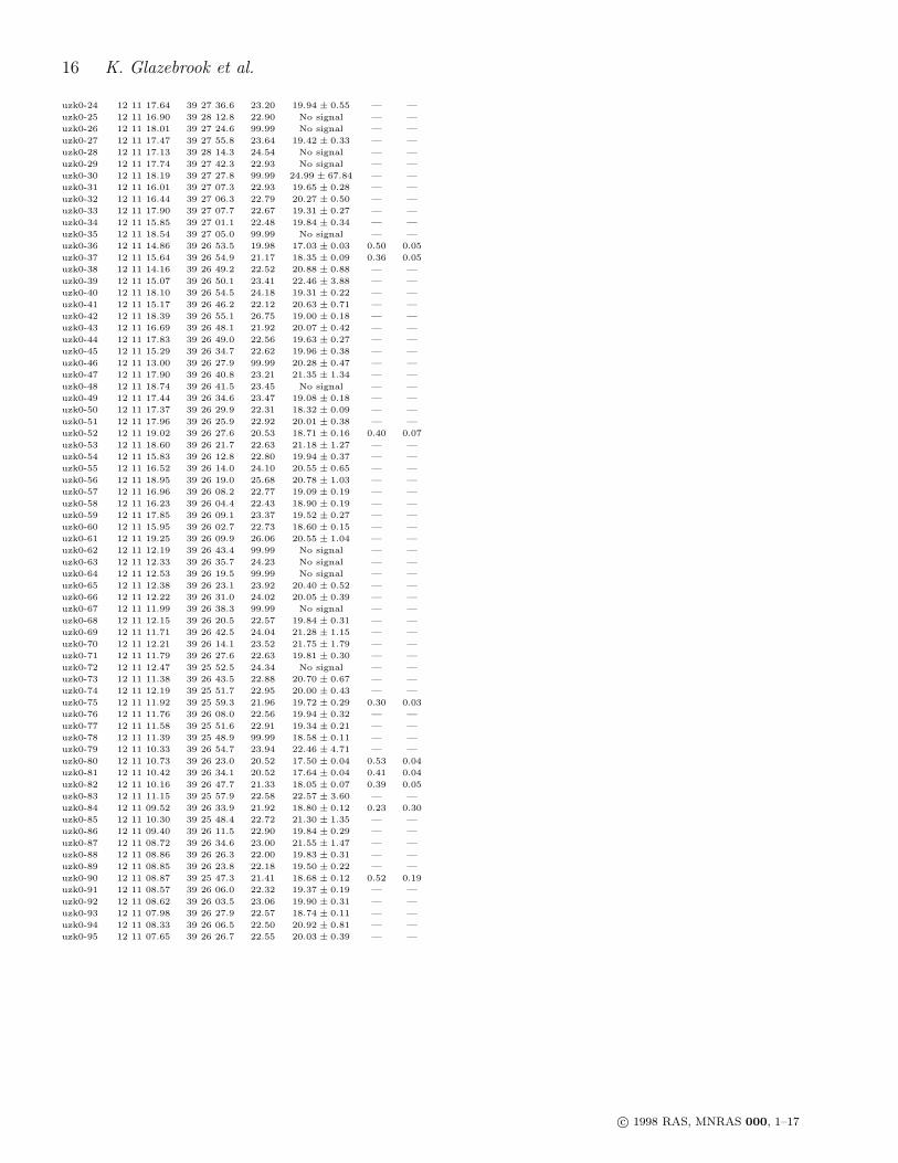
16 K. Glazebrook et al.

uzk0-24 12 11 17.64 39 27 36.6 23.20 19.94 ± 0.55 — —

uzk0-25 12 11 16.90 39 28 12.8 22.90 No signal — —

uzk0-26 12 11 18.01 39 27 24.6 99.99 No signal — —

uzk0-27 12 11 17.47 39 27 55.8 23.64 19.42 ± 0.33 — —

uzk0-28 12 11 17.13 39 28 14.3 24.54 No signal — —

uzk0-29 12 11 17.74 39 27 42.3 22.93 No signal — —

uzk0-30 12 11 18.19 39 27 27.8 99.99 24.99 ± 67.84 — —

uzk0-31 12 11 16.01 39 27 07.3 22.93 19.65 ± 0.28 — —

uzk0-32 12 11 16.44 39 27 06.3 22.79 20.27 ± 0.50 — —

uzk0-33 12 11 17.90 39 27 07.7 22.67 19.31 ± 0.27 — —

uzk0-34 12 11 15.85 39 27 01.1 22.48 19.84 ± 0.34 — —

uzk0-35 12 11 18.54 39 27 05.0 99.99 No signal — —

uzk0-36 12 11 14.86 39 26 53.5 19.98 17.03 ± 0.03 0.50 0.05

uzk0-37 12 11 15.64 39 26 54.9 21.17 18.35 ± 0.09 0.36 0.05

uzk0-38 12 11 14.16 39 26 49.2 22.52 20.88 ± 0.88 — —

uzk0-39 12 11 15.07 39 26 50.1 23.41 22.46 ± 3.88 — —

uzk0-40 12 11 18.10 39 26 54.5 24.18 19.31 ± 0.22 — —

uzk0-41 12 11 15.17 39 26 46.2 22.12 20.63 ± 0.71 — —

uzk0-42 12 11 18.39 39 26 55.1 26.75 19.00 ± 0.18 — —

uzk0-43 12 11 16.69 39 26 48.1 21.92 20.07 ± 0.42 — —

uzk0-44 12 11 17.83 39 26 49.0 22.56 19.63 ± 0.27 — —

uzk0-45 12 11 15.29 39 26 34.7 22.62 19.96 ± 0.38 — —

uzk0-46 12 11 13.00 39 26 27.9 99.99 20.28 ± 0.47 — —

uzk0-47 12 11 17.90 39 26 40.8 23.21 21.35 ± 1.34 — —

uzk0-48 12 11 18.74 39 26 41.5 23.45 No signal — —

uzk0-49 12 11 17.44 39 26 34.6 23.47 19.08 ± 0.18 — —

uzk0-50 12 11 17.37 39 26 29.9 22.31 18.32 ± 0.09 — —

uzk0-51 12 11 17.96 39 26 25.9 22.92 20.01 ± 0.38 — —

uzk0-52 12 11 19.02 39 26 27.6 20.53 18.71 ± 0.16 0.40 0.07

uzk0-53 12 11 18.60 39 26 21.7 22.63 21.18 ± 1.27 — —

uzk0-54 12 11 15.83 39 26 12.8 22.80 19.94 ± 0.37 — —

uzk0-55 12 11 16.52 39 26 14.0 24.10 20.55 ± 0.65 — —

uzk0-56 12 11 18.95 39 26 19.0 25.68 20.78 ± 1.03 — —

uzk0-57 12 11 16.96 39 26 08.2 22.77 19.09 ± 0.19 — —

uzk0-58 12 11 16.23 39 26 04.4 22.43 18.90 ± 0.19 — —

uzk0-59 12 11 17.85 39 26 09.1 23.37 19.52 ± 0.27 — —

uzk0-60 12 11 15.95 39 26 02.7 22.73 18.60 ± 0.15 — —

uzk0-61 12 11 19.25 39 26 09.9 26.06 20.55 ± 1.04 — —

uzk0-62 12 11 12.19 39 26 43.4 99.99 No signal — —

uzk0-63 12 11 12.33 39 26 35.7 24.23 No signal — —

uzk0-64 12 11 12.53 39 26 19.5 99.99 No signal — —

uzk0-65 12 11 12.38 39 26 23.1 23.92 20.40 ± 0.52 — —

uzk0-66 12 11 12.22 39 26 31.0 24.02 20.05 ± 0.39 — —

uzk0-67 12 11 11.99 39 26 38.3 99.99 No signal — —

uzk0-68 12 11 12.15 39 26 20.5 22.57 19.84 ± 0.31 — —

uzk0-69 12 11 11.71 39 26 42.5 24.04 21.28 ± 1.15 — —

uzk0-70 12 11 12.21 39 26 14.1 23.52 21.75 ± 1.79 — —

uzk0-71 12 11 11.79 39 26 27.6 22.63 19.81 ± 0.30 — —

uzk0-72 12 11 12.47 39 25 52.5 24.34 No signal — —

uzk0-73 12 11 11.38 39 26 43.5 22.88 20.70 ± 0.67 — —

uzk0-74 12 11 12.19 39 25 51.7 22.95 20.00 ± 0.43 — —

uzk0-75 12 11 11.92 39 25 59.3 21.96 19.72 ± 0.29 0.30 0.03

uzk0-76 12 11 11.76 39 26 08.0 22.56 19.94 ± 0.32 — —

uzk0-77 12 11 11.58 39 25 51.6 22.91 19.34 ± 0.21 — —

uzk0-78 12 11 11.39 39 25 48.9 99.99 18.58 ± 0.11 — —

uzk0-79 12 11 10.33 39 26 54.7 23.94 22.46 ± 4.71 — —

uzk0-80 12 11 10.73 39 26 23.0 20.52 17.50 ± 0.04 0.53 0.04

uzk0-81 12 11 10.42 39 26 34.1 20.52 17.64 ± 0.04 0.41 0.04

uzk0-82 12 11 10.16 39 26 47.7 21.33 18.05 ± 0.07 0.39 0.05

uzk0-83 12 11 11.15 39 25 57.9 22.58 22.57 ± 3.60 — —

uzk0-84 12 11 09.52 39 26 33.9 21.92 18.80 ± 0.12 0.23 0.30

uzk0-85 12 11 10.30 39 25 48.4 22.72 21.30 ± 1.35 — —

uzk0-86 12 11 09.40 39 26 11.5 22.90 19.84 ± 0.29 — —

uzk0-87 12 11 08.72 39 26 34.6 23.00 21.55 ± 1.47 — —

uzk0-88 12 11 08.86 39 26 26.3 22.00 19.83 ± 0.31 — —

uzk0-89 12 11 08.85 39 26 23.8 22.18 19.50 ± 0.22 — —

uzk0-90 12 11 08.87 39 25 47.3 21.41 18.68 ± 0.12 0.52 0.19

uzk0-91 12 11 08.57 39 26 06.0 22.32 19.37 ± 0.19 — —

uzk0-92 12 11 08.62 39 26 03.5 23.06 19.90 ± 0.31 — —

uzk0-93 12 11 07.98 39 26 27.9 22.57 18.74 ± 0.11 — —

uzk0-94 12 11 08.33 39 26 06.5 22.50 20.92 ± 0.81 — —

uzk0-95 12 11 07.65 39 26 26.7 22.55 20.03 ± 0.39 — —

c© 1998 RAS, MNRAS 000, 1–17

Physical parameters of faint galaxies 17

TABLE 3. Statstical comparison of I − K distribution with models.

Model All E/S0log PKS XS Med log PKS XS Med

No-Evolution SEDs Ω = 0 -12.67 1.60 2.85 -6.95 2.23 3.20No-Evolution SEDs Ω = 1 -12.30 1.99 2.85 -7.09 3.08 3.25PBZ Luminosity Evolution Ω = 0 -2.88 1.36 2.60 -6.52 1.34 3.25PBZ Luminosity Evolution Ω = 1 -1.54 1.52 2.50 -6.94 1.32 3.35

Model Spiral Irr/Peclog PKS XS Med log PKS XS Med

No-Evolution SEDs Ω = 0 -6.45 0.90 2.80 -4.81 5.87 2.45No-Evolution SEDs Ω = 1 -6.37 1.10 2.80 -4.45 6.96 2.45PBZ Luminosity Evolution Ω = 0 -3.27 0.88 2.50 -8.65 4.63 2.10PBZ Luminosity Evolution Ω = 1 -5.69 1.04 2.40 -8.68 5.22 2.05‘Eternally Middle-Aged’ (Ω = 1) — — — -2.73 1.83 2.55

c© 1998 RAS, MNRAS 000, 1–17