The phenology of crops and the development of pests and ...

The phenology of crops and the development of pests and diseases

Literature, research, models and future

operational integration

T.H. Sivertsen, P. Nejedlik, R. Oger and R. Sigvald

Rapport 1/99

ISBN 82 – 479 – 0125 – 0

ISSN 0809- 182x

1999

THE PHENOLOGY OF CROPS AND THEDEVELOPMENT OF PESTS AND DISEASES

COST 711

The operational applications of meteorology to agriculture, including horticulture

A report from a working group on phenology, pests and deseases on crops

Sivertsen, T. H.Nejedlik, P.Oger, R.Sigvald, R.

Literature, research, models and future operational integration

1

Acknowledgements ...........................................................................................................................3 1. INTRODUCTION.................................................................................................................4

1.1 The initiation of the report writing ....................................................................................4 1.2 The aims of the report writing..........................................................................................4 1.3 The agriculture, vegetation, and climate in the geographical region covered by the report and the choice of crops for this study...................................................................................................5 1.4 Research and operational utilisation of research ....................................................................6 1.5 What is phenology?..........................................................................................................6

References ................................................................................................................................7 2. PLANT DEVELOPMENT....................................................................................................9

2.1. Description of crop phenology ...............................................................................................9 2.1.1. General features ............................................................................................................9 2.1.2. Cereals, winter wheat and spring barley.....................................................................9 2.1.3 Potato.............................................................................................................................11

2.2. Development scales.............................................................................................................14 2.2.1 Development scales of cereals.....................................................................................14 2.2.2 Development scales of potato.......................................................................................18

2.3 Responses of crop phenology to environmental conditions ..................................................22 2.3.1.Temperature .................................................................................................................22 2.3.2 Photoperiod...................................................................................................................25 2.3.3. Vernalisation................................................................................................................27 2.3.5. Nitrogen stress ............................................................................................................30

3. PESTS AND DISEASES ....................................................................................................33 3.1 Influence of environmental conditions on plant pests ...........................................................33

3.1.1 Introduction ..................................................................................................................33 3.1.2 Temperature .................................................................................................................33 3.1.3 Precipitation and moisture ..........................................................................................34 3.1.4 Wind ..............................................................................................................................34

3.2 Influence of environmental conditions on plant diseases ....................................................34 3.2.1 The pathogen, the host and the environment.............................................................34 3.2.3 Effect of temperature ...................................................................................................35 3.2.4 Effect of moisture .........................................................................................................35 3.2.5 Effect of wind ................................................................................................................36 3.2.7 Effect of light.................................................................................................................36 References and additional readings .....................................................................................36

4. EFFECTS OF PESTS AND DISEASES ON CROP ..................................................................38 4.1. Introduction .....................................................................................................................38 4.2. Effects on crop growth .........................................................................................................38 4.3 Susceptible phenological stages ............................................................................................38

5. OVERVIEW OF PHENOLOGICAL MODELS ........................................................................41 5.1 Winter wheat and barley .......................................................................................................41

5.1.1 General principles and concepts .................................................................................41 5.1.2 AFRC Wheat phenological submodel.........................................................................41 5.1.3 SUCROS development subroutine..............................................................................43 5.1.4 WOFOST Crop simulation model ..............................................................................44 5.1.5 Ceres Wheat..................................................................................................................45

5.2. Potato ..............................................................................................................................47 5.2.1 General principles ........................................................................................................47 5.2.2 A Simple Model of Potato Growth and Yield (England) ..........................................48 5.2.3 DAISY model ................................................................................................................49

6. OVERVIEW OF PEST AND DISEASE MODELS OF WINTER WHEAT, BARLEY AND POTATOES ....................................................................................................................................53

6.1 Introduction ...........................................................................................................................53 6.2 Literature survey on models (selected pests and diseases) ....................................................53

6.2.1 Cereals ...........................................................................................................................53 6.2.2 Potatoes .........................................................................................................................58 Additional references and additional readings ..................................................................62

6. OVERVIEW OF PEST AND DISEASE MODELS OF WINTER WHEAT, BARLEY AND POTATOES ....................................................................................................................................63

2

6.1 Introduction ...........................................................................................................................63 6.2 Literature survey on models (selected pests and diseases) ....................................................63

6.2.1 Cereals ...........................................................................................................................63 6.2.2 Potatoes..........................................................................................................................68 Additional references and additional readings ..................................................................72

8. Limitation of existing models......................................................................................................73 8.1. Generally about models and modelling ................................................................................73

8.1.1. What is a model? .........................................................................................................73 8.1.2. The hypothetico-deductive method in some detail....................................................73 8.1.3. Parametrization and scale considered .......................................................................74

8.2 Meteorological data ...............................................................................................................75 8.2.1 Sources of the meteorological data to be used in models...........................................75 8.2.2 The quality of the meteorological data ................................................................76 8.2.3 Accuracy and representativeness of meteorological data..................................77 8.2.4 Control of meteorological data ....................................................................................77 8.2.4 Interpolation, extrapolation, and estimation of meteorological data ................78 8.2.6 Estimation of meteorological data at the canopy level and in the air above the station .....................................................................................................................................78

8.3 Requirement for the accuracy of the models .........................................................................80 8.3.1. Crop development models...........................................................................................80

8.3.2 Accuracy of Pest and Disease Models................................................................................84 8.4. Calibration and validation of the models.........................................................................85

8.4.1 Generally about phenological models of crops..........................................................85 8.4.2 Validation of crop development models..............................................................86 8.4.3 Validation of Pest and Disease Models .......................................................................88

9.What kind of work is needed in the future?..................................................................................91

3

Acknowledgements The whole working group would like to thank the chairman of COST 711 Martin Hims, England, as well as the former secretary of COST 711, Jean Labrousse, who initiated this report and together with Richard Delecolle, France, made the first plan forthis work. Martin Hims has also read the report and has done a substantial job in correcting the English. The group on phenology also wish to thank Mrs.Sirpa Kurppa, Finland, who originally was a member of the group and did much of the first editing of this report. Tor H. Sivertsen would like to thank Sofus L. Lystad and Jan E. Haugen, Norwegian Meteorological Institute, Arne Hermansen, Norwegian Crop Research Institute, for providing references and other useful information for chapter 8, and Håkon A. Magnus and Halvard Hole, Norwegian Crop Research Institute, for providing a colour picture and constructing the front page of the report. Håkon A. Magnus has also read the report and has been helpful in correcting errors. P. Nejedlik would like to thank the authors A. Bussay and C. Szinell, Hungary, for the use of data in table 8.4

4

1. INTRODUCTION

1.1 The initiation of the report writing The writing of this report was initialised by the management committee of the COST ACTION 711 Operational Applications of Meteorology to Agriculture, including horticulture. The management committee established a working group to study and write a report on the phenology of crops and the development of pests and diseases. The members of this working group were all national delegates in the management committee, and the group consisted of the following persons: Mr. Tor H. Sivertsen, Norwegian Crop Research Institute, Ås, Norway Mr. Robert Oger, Centre de Recherches Agronomiques, Station de Phytopathologie, Gembloux, Belgium Mr. Pavol Nejedlik, Slovak Hydrometeorological Institute, Bratislava, Slovakia Mr. Roland Sigvald, Swedish University of Agricultural Sciences, Uppsala, Sweden T. H. Sivertsen has done the editing of the report and written chapter 1, minor parts of paragraphs 2.1.2 and 2.2.1.1, paragraphs 8.1, 8.2.1, 8.2.2, 8.2.3, 8.2.4, 8.2.5 , parts of paragraph 8.2.6, and chapter 9. R. Oger has written 2.1, most of paragraphs 2.1.2 and 2.2.1, the paragraphs 2.3.1.1, 2.3.2.1, 2.3.3,1, 2.3.4.1, 2.3.5,1, 5.1, chapter 7, parts of paragraphs 8.2.6, and paragraph 8.4.1. P. Nejedlik has written paragraphs 2.1.3, 2.2.2, 2.3.1.2, 2.3.2.2, 2.3.4.2, 2.3.5.2, 8.3.1, and 8.4.2. R. Sigvald has been the leader of a Swedish group consisting og himself, Björn Andersson, Annika Djurle, Mats Lindblad, Magnus Sandström, Eva Twengström, and Jonathan Juen. This group has written chapter 3, chapter 4, chapter 6, and paragraphs 8.3.2 and 8.4.3.

1.2 The aims of the report writing The foundation of the COST ACTION 711 is found in the memorandum of understanding signed by all member countries of the management committee. According to the memorandum of understanding the main objectives of the project would be to achieve major economic benefits by the better utilisation of the simulation and understanding of combined biological, geophysical and atmospheric processes in operational weather services. One of the ways of achieving these objectives can accrue from the availability of developing accurate models for forecasting the occurrence and intensity of plant and animal diseases, and constructing trajectory models which facilitate emergency action in the face of occasional outbreaks of particularly virulent airborne infections. Topics especially mentioned in the memorandum of understanding are: ‘Pest and disease prediction schemes based on fundamental understanding of pathogen life-cycles - and crop micro-meteorology - and plant protection based on weather data’ The objectives of this written report are, through a combined study of the literature, existing models of phenology of some major agricultural crops and the development of pests and diseases of these crops, to clarify: (a) The existence of useful models. (b) How it may be possible to use the existing models operationally in plant protection? (c) How should future research and development be organised to improve existing operational models and construct new operational models in this context?

5

1.3 The agriculture, vegetation, and climate in the geographical region covered by the report and the choice of crops for this study The geographical context of COST ACTION 711 are the countries of the European Union, Hungary, Slovakia, Slovenia, and Norway, in short Western, Northern, and Central Europe from 37°N to 70°N and between 10°W and 20°E, with some Eastern European countries inside this area excluded. This region consists, in the global sense, of technically advanced industrialised countries with mainly commercial agricultural production. The following three types of agriculture are found in this region: Commercial dairy agriculture, commercial arable and extensive horticultural crop production and livestock agriculture, and mediterranean agriculture. Commercial intensive agriculture is also found in certain specialised locations or regions. Crop production in mediterranean agriculture reflects the climate of this region and it consists of crops which yield early in the season, crops which withstand dry summers without irrigation, and crops which benefit from irrigation. Cereals and other arable non-cereal field crops, tree crops, grapes, field and protected vegetables, top and fruit crops are produced (Thoman, et al., 1968). There are several climatic types in the region, Mediterranean subtropic (dry summer) in the south, highlands in the Alps and in some other mountainous areas, marine (cool summer) in the west and north west, and humid continental mainly in the north east (Thoman, et al., 1968). The original natural vegetation of the region consists both of Mediterranean maquis, chaporal or shrubs intersperced with grasses in the south, broadleaf and mixed broadleaf- coniferous forest in the central part of the region, and coniferous forests in the north and in mountainous areas. There are many different soil types in this region, both alluvial soils, morainic deposits, and other soils of mountainous areas, as well as marine deposits are found. Substantial areas are covered with grey-brown forest soil in the central part and podzol in the north (Thoman, et al., 1968). The crops chosen to be studied in this report are a few of the main agricultural and horticultural crops of the region or better parts of the region; Winter wheat, spring barley, and potato. Wheat (genus Triticum) and barley (genus Hordeum) are both cereals of the Graminea family. Wheat and barley are known to be cultivated as early as 7500-6500 BC in th Middle East. Both the ancient Mesopotamian and the Egyptian cultures were growing these cereals in irrigated fields from about 5000 BC. In the Balkans wheat was probably cultivated from about 6000 BC, and farming of cereal crops had spread to the Iberian peninsula at 4500 BC, reached the North Sea before 4000 BC and the British Isles around 3500 BC (Russel, 1990; Russel and Wilson, 1994). Wheat and barley are the most important and the second most important cool temperate cereals in the world (Russel, 1990). The main growing area of these cereals in the northern hemisphere is between 30° N and 60° N, but it is possible to grow barley in Norway at 70° N well beyond the arctic circle. Barley tends to replace wheat where the annual precipitation is too low or too erratic or where the growing season is too short for wheat. Wheat and rice are foremost among cereals as direct food sources for human beings, but much wheat is also used for fodder in animal husbandry. In Europe barley is now mainly used to fatten cattle or in the brewing and distilling industries. In Scandinavian mountain valleys barley in former days was grown as an important food crop for human consumption, often used as porridge. More information about wheat and barley, their history, biology, and present cultivation systems in Europe may be found in (Russel, 1990) and (Russel and Wilson, 1994).

Potato belongs to the genus Solanum. The wild species of potato still occur in its original home in three regions of the South America: The Andes mountain region in Peru and lowland centres in Chile and Uruguay. According to many authors (Salaman, 1949,Vavilov, 1960) the predecessor of European varieties of potato, Solanum tuberosum, originated in Chile lowland region and nearby islands. The wild species of potato in this subtropical region are long-day or neutral photoperiod reactive and reproduce by generative seeds. The potato of Andean origin is a short-day photoperiod reactive species. Both cultural species of Solanum tuberosum and Solanum

6

andigenum are tetraploid. Cultivation has increased tuber size and reduced the content of poisoned and bitter ingredients.

The potato crop is grown for tubers, production which have three principal uses:

- food, direct consumption or for making food products

- industrial use, mainly to produce starch and alcohol

- fodder for animals

1.4 Research and operational utilisation of research The type of operational systems considered in this report, consist of the gathering and use of meteorological data and biological data (crops, plant pests, and plant diseases), the production of warnings and advice, and the dissemination of this information to the farmers and growers as well as other elements of the agricultural and horticultural industries. One could be inclined to ask which operational systems exists and which relevant research activities to create such systems are going on in Europe and in other regions of the world? By writing this report we are in fact trying to give an answer to this question, but our answer in the report will by, no means be complete. The following areas of research are involved in creating operational systems for crop protection: Meteorology, agrometeorology, entomology, plant pathology, plant physiology, agronomy, soil sciences, horticultural and crop sciences. Research activities covered by other COST actions are relevant in this context: COST ACTION 66: Pesticides - Soil- Environment COST ACTION 75: Advanced weather radar systems COST ACTION 77: Application in remote sensing in agrometeorology COST ACTION 78: Development of nowcasting techniques COST ACTION 79: Integration of data and methods in agroclimatology COST ACTION 816: Biological control of weeds in Europe COST ACTION 817: Population studies of airborne pathgens on cereals as a means of improving strategies for disease control COST ACTION 823: New technologies to improve phytodiagnoses

1.5 What is phenology? The origin of the word phenology are the greek words fainesthai (φαινεσθαι), to appear, and logos (λóγος), reason. Lieth, (1970), defines phenology in the following way: ‘Phenology is generally described as the art of observing life cycle phases or activities of plants and animals in their temporal occurence throughout the year.’ The US International Biological Program Phenology Committee(1972) gave the following definition of phenology: ‘Phenology is the study of the timing of recurring biological events, the causes of their timing with regard to biotic and abiotic forces, and the interaction among phases of the same or different species.’ The US IBP committee added to this:

‘The unit of study may vary from a single species (or variety, clone, etc.) to a complete ecosystem. The area involved may be small (for intensive studies on all phenophases of entire ecosystems) or large (for interregional comparison of significant phenophases). The unit of time is usually the solar year with which the events to be studied are in phase. The events themselves may cover variable time spans, often much shorter than the solar year.’

7

In this report we will concentrate on the phenology of agricultural crops and their pests and diseases. The aim of the report is to show to what extent phenological models (scientific hypotheses) of the development of a few agricultural crops and their pests and diseases exist, and how these models are validated and tested. The models should ideally be directly dependent on measurable quantititative meteorological variables such as air temperature, leaf temperature, daily photoperiod, leaf wetness, the humidity of the soil and the air etc.(Hodges,1991) The system we are considering consists of the atmosphere near the ground, the crops, the soil, and the pests and diseases of the crops. We must consider both the spatial and temporal changes of this system. Our system is in the biological sense a subsystem of a greater and more complex ecosystem. The more complete system consists of a description of individuals, population and communities of plants and animals etc., as well as the physics of the atmosphere and the soil, (Begon, Harper and Towsend, 1990). We have used traditionally scientific methods of describing the system using quantitative parameters for both the biotic and the abiotic parts of it. We also attempted to provide quantitative prognoses of the developement of the system in time and the phenological models which have to be tested by comparing measurements of observable facts to the output of the models. The definition and use of parameters is not always straightforward in such systems, (Elston and Monteith, 1975). One of the aims of scientific work like this is to develop decision support systems for the growers of agricultural and horticultural crops. By understanding the crop ecosystems and by giving forecasts of their quantitative development and their pests and diseases it is possible to give advice to the growers during the growing season based on predictions.

References Begon, M., Harper, J. L. and Towsend, C. R. (1990) Ecology, 945 pp, Blackwell Scientific Publications Elston, J., and Monteith, J. L., (1975) Micrometeorology and Ecology, in Vegetation and the Atmosphere,Volume 1, Academic Press, London, New York, San Fransisco Hodges, Tom, ed. (1991) Predicting crop phenology, Boca Raton, Fla.: CRC Press, 223 pp. Lieth, H. ed, (1974) Phenology and Seasonality Modeling, Ecological Studies, v.8, Springer- Verlag, New York, 444pp Lieth, H. (1970) Phenology in productivity studies, p.29. In Analysis of Temperate Forest Ecosystems, D. Reichle, ed. Hedelberg: Springer Verlag Russel, G. (1990), Barley knowledge base, in the series ‘ An agricultutrsal information system for the European community’, Joint Research Centre, European Commission, Italy Russel, G. and Wilson, G. W. (1994) An agro-pedo climatological knowledge-base of wheat in Europe, in the series ‘ An agricultutrsal information system for the European community’, Joint Research Centre, European Commission, Italy Salaman, R. N. (1949) The history and social influence of the potato, Cambridge Thoman, R. S., Concling, E. C., and Yeates, M. H. (1968) The geography of economic activity, McGraw-Hill Series in Geography, New York

8

US/IBP Phenology Committee (1972) Report, July 1972, 54 pp. offset. Austin, Texas: US/IBP Environmental Coordinating Office Vavilov, N. I. (1960) Collected papers in 5 parts. Problems of selection. Task of Euroasia and New World in the origin of cultural plants. Moskva- Leningrad, Akademia Nauk USSR. (In Russian)

9

2. PLANT DEVELOPMENT

2.1. Description of crop phenology

2.1.1. General features In general, phenology refers to the changes in the life stages of biological organisms and more precisely to the study of the timing of biological events, the causes of their timing with regard to biotic and abiotic forces, and the interrelations among them. Development of plants has been defined as a sequence of phenological events controlled by external factors , each event making important changes in morphology and in partitioning of assimilates among different organs during the plant’s life-cycle. In this context, the rate of phenological development may be defined as the reciprocal of the time required for the organism to progress from one stage to the next. The purpose of phenological studies in an agricultural and horticultural context is to facilitate planning of operations, such as irrigation, the application of fertilisers and pesticides, the timing of which is dictated by the occurrence of a particular stage of crop, pest or disease development. To facilitate modelling it has become a common place to analyse crop response to environment factors as a series of steps rather than a continuous response. Most of models defines key phases and take into account the direct effect of environmental variables during each phase and when possible the memory effect of these variables from phase to phase.

2.1.2. Cereals, winter wheat and spring barley In cereals three principal phases are generally recognised during crop development: the vegetative, the reproductive and the maturation phases. The vegetative phase of cereals lasts until the stem apex converts from producing vegetative nodes to producing reproductive nodes each of which subtends a spikelet. The double ridges stage is the first directly observable indication that reproductive development has begun. During the reproductive phase, tiller buds and roots cease extension, tiller abortion is induced. Within the reproductive phase, the yield components, spikelet number, kernel number and kernel weight are determined. The period between pre-anthesis ear growth and physiological maturity is called the maturation phase. Vegetative phase In most European countries, sowing of winter wheat are normally made during the period September to December and in any region, a wide range of sowing dates may be observed. Spring barley is sown during the period February-April in most of Europe, but as late as the beginning or the middle of May in northern parts and in mountain valleys. The date of sowing in each field depends on the suitability of the soil for cultivation, the date of harvest of the previous crop, the soil temperature and on the farmer's priorities for sowing. Autumn sown winter wheat gives a mean cycle length from sowing to harvest which varies between 250 to 300 days. Spring sowings of barley give a cycle length from sowing to harvest of 130 days ( range 90- 180 days). After sowing the vegetative phase of the plant starts with the imbibition and the germination of the seed. Germination is essentially the emergence of the root and coleoptile of the caryopsis. Crop emergence can be defined in several ways, but from a functional point of view the best definition is probably the date when 50% of the plants are emerged with one unfolded leaf visible. In normal circumstances, there is only a delay of a few days between the emergence of the first and last plants. During winter the apex of winter wheat develops slowly. In spring, important changes occur on the stem apex during the seedling growth phase. The seedling period of spring sown barley is of course much shorter than for winter sown cereals. The organs of the cereal shoot are initiated at the shoot apex. For much of the life cycle of the cereal plant this is at or just below soil level and surrounded by leaves so that the changes at the growing point can only be studied by techniques such as serial sectioning (Kirby, 1974) or dissection. Study of the shoot apex in this way provides

10

information about initiation of flowering and the development of the ear which cannot be seen by external inspection but which is nevertheless important in both husbandry and fundamental research. External morphological changes are characterised by seedling growth, successive leaf appearance and tillering. Leaf primordia are initiated in sequence on the stem apex followed by spikelet primordia. Initially all primordia are undifferentiated and cannot easily be distinguished morphologically. During this phase most of the leaves appear.The number of main stem leaves initiated before the onset of reproductive development varies with date of sowing and cultivar. The number of leaves increases with an early autumn sowing and an incomplete vernalisation for winter wheat. The thermal time between the appearance of successive leaves is called the phytotherm and appears to be constant for each sowing date and location. Kirby, Appleyard & Fellowes (1985) found that the rate of leaf appearance was related to the rate of change of day length at crop emergence although it is not known whether this relationship is directly causal or whether it hides a more complex relationship with photoperiod. Leaf development is strongly related to phenology in a number of ways. The total number of leaves of a given shoot and rate of appearance are directly related to the duration of the development interval to floral initiation as well as to the rate of leaf primordia initiation. Once final leaf number is determined, these leaves emerge before the flower becomes visible and anthesis occurs. An important feature of the development of the cereal plant is its ability to produce tillers, i.e. lateral stems. A tiller bud develops in the axil of the coleoptile and each of the lower leaves of the plant. The proportion of buds which actually develop into tillers depends on genotype and environment, particularly the irradiance and nitrogen status. Tillering generally starts after the appearance of the fourth leaf, more than 150 days after emergence in winter wheat sown in late autumn. Since tillers produce fewer leaves than the main stems, ear emergence takes place almost synchronously over the whole population of stems (Kirby & Appleyard, 1984). Tillering enables the plant to respond to variation in density of sowing. Similar responses in tiller numbers are caused by variation in genotype, nutrient levels, water supply and plant growth regulators. The number of ears per plant is an important yield component, and thus the timing of tiller production and the number and final size of tillers have critical effects on final grain yield. Table 2.1 Relative importance of development phase on yield components of winter wheat Development phase Plant/m² Ears/plant Grains/ear 1000grains weight Total biomass

Sowing to emergence

+++ - - - -

Emergence to floral initiation

- +++ - - +

Floral initiation to terminal spikelet

- ++ + - +++

Terminal spikelet to heading

- + +++ - +++

Heading to anthesis - - ++ + +++

Anthesis to maturity - - + +++ ++

During the vegetative phase the sinks for assimilate are the leaves and the roots. After the onset of the reproductive phase, the growing stem also becomes a sink. The developing ear is a minor sink in terms of assimilate requirement since it only makes a small part of the total biomass at flowering.

11

Reproductive and maturation phase The transition to reproductive growth is marked by a pronounced increase in the rate of primordium initiation. The problem of predicting the transition between these two phases of development on the stem apex has not yet been solved completely although there is now a considerable literature on this subject. One of the morphological indications is the appearance of double ridges on the upper spikelet but the transition can be identified by an increase in the rate of initiation of primordia. Reproductive growth proceeds until new primordia cease to be initiated. During this phase, the spikelet number declines till the final number of grains per ear is reached at ear emergence. Stem extension occurs due to the elongation of the upper five or six internodes of the stem. The end of stem elongation phase is marked by the emergence of the flag leaf and its ligule. Booting starts with the extension of the flag leaf sheath until the first spikelets are visible. The reproductive phase finishes with the inflorescence emergence and anthesis. Flowering or anthesis dehiscence of the anthers and pollen shedding onto the receptive stigmas of the carpel, is a key stage in the development of the cereals. Following successful anthesis, the grain begins to fill and passes through successive stages from milk to hard dough. During this time there is a progressive senescence of the leaves followed by the glumes of the ear. The grain dry weight reaches a maximum at the end of the dough stage. With the reproductive phase, the yield components, spikelet number, kernel number and kernel weight are finally determined.

2.1.3 Potato

The systematic classification of potato varieties was firstly based on the length of the period of vegetation (19th century), later on the biological features (Danert, 1965). The quality of the tubers and the seasonal accessibility of the crop are often used as criteria for classification of poato.

Potato crops may be divided into two different groups based on the period of vegetative growth and the economical use:

1. food cultivars

- very early and early cultivars

- semi-late and late cultivars

2. cultivars for industrial use

- semi-late and late cultivars

It is possible to propagate the potato both in generative and vegetative way. Under generative reproduction a bud is growing out of the seed together with side roots. Afterwards, under the ground, tubers are grown on the top of stolons. But for potato multiplication vegetative propagation is highly predominant. From the botanical point of view potato is a perennial plant, (so called great cycle), that is every year vegetatively propagated by producing new tubers (little cycle). Buds on the tubers germinate to produce stems above the ground and roots and new tubers in the soil. The development of individual potato clusters is equivalent to the ontogenesis of an annual plant. The cycle of vegetative propagation starts at harvest, when the tuber is separated from the potato cluster. The following period is one of endogenous and exogenous dormancy. In this period of crypto- vegetative growth the tubers utilise the stored nutrients. During dormancy biochemical processes continue within bud tissue. To maintain an appropriate time interval, endogenous dormancy is regulated by the relative quantities of plant growth hormones. During this period the plant does not germinate even under favourable temperatures. Exogenous dormancy is mostly regulated by temperature. Germination starts at 5-8 ºC and exhibits a pre-root and root stage.

The continent of Europe belongs mostly to the cool and warm temperate zone. Under these climatic conditions it is principally temperature that limits the lenght of the growing season. The need to avoid late spring frosts causes planting delays from the south to the north. The need to

12

minimise or escape leaf, stem and tuber infection by Phytophtora infestant and early autumn frosts determines the end of the season.

The interval of the period of vegetation varies widely according to the variety approximately from 90 to 180 days. There are many standard descriptions of growth stages of the crops. Plant behaviour is a function of many factors. Climatic, pedological and geomorphologic factors determine plant growth. Each group of varieties responses to the environment differently. According to the length of the period of vegetation the varieties can be classified into three groups:

-early varieties ( 90-120 days)

-medium varieties (120-150 days)

-late varieties (150-180 days)

The length of the subperiods of the vegetative period is also different, of course. Doorenbos and Kassan (1979) recognised four main phases of the vegetative period:

-period of establishment (15-25 days), when the plant depends on substrates from the mother tuber

-the vegetative phase (20-40 days), during which tuber initiation starts

-the yield formation period (45-60 days), during which tuber growth is predominant

-period of ripening (20-35 days) when the haulm gradually becomes senescent and dies

Phenological data register the results of plant development during its life. In the period of vegetation photosynthesis takes place in the green parts of the plant. Though the time span of the period of vegetation is usually shorter than the dormancy period the manifestation of life cycle is much more remarkable.

Since the potato is, with the exception of inter-variety breeding, propagated vegetatively the definition of vegetative, reproductive and maturation phase is not so well defined as it is in cereals. Varietes of the potato that are grown in the field abort the buds before opening, so plants do not flower and produce the berry (seed). The individual development of the potato comprise all the structural and functional changes of the organism. Clearly there are a number of biological differences in the production of new ‚individuals‘ by true seed formation compared to vegetative propagation. Since the latter is most often used, except of course for inter-variety breeding, only the former method will be considered in this report.

New plant development begins after the break of dormancy when the process of bud growth starts. This normally happens to seed potatoes in store and usually occurs when the sprouts reached ca 3 mm in length. In many European countries this happens usually between November and January. The sprout grows out from the buds situated in the ‘eyes’ of the seed and includes all parts of the plant in a rudimentary form - internode, apex bud, axillary buds. At the base of the sprout the roots and stolons are formed when the sprout reaches a length of 1,5 to 3 cm due to internode elongation. MacKerron (1992) distinguishes two phases in the process of sprouting, the formation of leaf primordia by deliminating internodes on the sprout and the extension of the internode.

The date of potato planting depends on many factors: Natural limits, type of soil, terrain slope and aspect, temperature and soil moisture etc. are more or less combined with the factors of farming technology, and the date of planting is strongly influenced by the variety from very early to late. The potato crop is spread across whole of Europe and is grown under quite different climatic conditions. These geographic and climatic influences more or less ensure that potato planting goes on during a major part of the year – from the beginning of December to mid-summer. While in Spain and Greece planting covers according to the variety and regional geographical and climatic features the period from early December to July in Central and Northern Europe the most favourable conditions are from mid-March to May. In the last decades this process is in many countries affected by government regulations. According to the break of dormancy the date of planting can occur before or after sprouting. In many cases, especially for early varieties, presprouting is widely used to prepare the seed for planting. The state of sprout development at the

13

time the seed is planted affects the rate of subsequent plant growth. This state can be described by using so called ‘Physiological Age’. This concept represents the sum of accumulated temperature above base 4oC from the moment of dormancy break. Physiological age varies quite widely. Sprouting is utilised mostly in early varieties that can reach physiological age at planting a few hundred oC, up to 1000oC in extremes. For unsprouted tubers the physiological age is zero.

During the first period from planting to emergence the process of development is fed by nutrients stored in the mother tuber. After emergence photosynthesis by above ground stems and leaves continues this process of nutrient provision. The emergence of the individual plant depends on its vitality and environmental conditions. The time period from planting to emergence covers the interval of a few weeks. Table 2.7 shows some results of the duration from planting to emergence. Generally, the date when 50 % of the plants have emerged is assigned to be the date of crop emergence. But the emergence as a process, as stem apex breaks the soil surface covers a time interval in field conditions. According to observations over 10 years in North Carpathians in various climatic conditions (stations from 105 to 940 m altitude) the interval between 10 and 100% of the emerged plants takes mostly 5 to 15 days but exceeds 20 days under unfavourable environmental conditions.

From a point of view of creating new propagative units the tuber initiation starts the process of vegetative propagation. The definition of this phase is not uniform and doubling of the diameter of the stolons is often taken as the beginning of tuber initiation. In many varieties this time is in accord with the period of bud swelling, though some exceptions are recognised. Finally, tuber initiation is not synchronised with any phenological phase in stems and leaves above ground. The timing of tuber initiation is an important period in determining the final crop yield. Environmental factors strongly influenced the number of tubers developing on one stem or per unit area. In general an accumulated temperature sum above 0°C from 580 to 650°C for unsprouted seed is that required for tuber initiation according to the variety (O’Brian et al 1983). The growth of tubers varies considerably according to variety. Even though many varieties do not produce true seed, intensive tuber growth is frequently associated with flowering and berry fruit development.

The start of the senescence characteristics the end of the period of the potato cluster. At this stage the majority of the products of photosyntesis are transferred into the daugther tubers. Individual development of the potato stops with haulm death. Despite this biological fact harvest frequently advances haulm death in early varieties. Chemical, or mechanical destruction of the haulm is often used to accelerate maturation of the tubers. During the whole period of vegetation farming activities are required. Some of them are connected just to potato crop development though other activity is also necessary. Fig. 2.1 summarize some of the agricultural works with respect to crop development.

FARMING ACTIVITY

- field cultivation

- fertilization

- potato-seed preparation - pest and diseases protection - crop cultivation (haulm destroy) - irrigation (if)

dormancy planting emergence flowering haulm death

Fig. 2.1. Farming activities during the cycle of vegetation at potato.

14

2.2. Development scales

2.2.1 Development scales of cereals 2.2.1.1 Plant morphology based development scales of cereals Growth and development in cereal plants does not proceed at a constant or fixed rate through time. They are modified by environmental factors like temperature, light intensity and duration, nutrition and husbandry techniques. Therefore, calendar date is not suitable for the quantitative description of the developmental stage of plants. Plant development is recognised as a complex series of events and is difficult to determine and to describe in a unified and comprehensive manner. There. have been many attempts to define precise and easily applicable methods for describing all the important periods and stages during cereal development. For husbandry purposes development of cereals have been segmented into periods or stages based on the description of exterior and visible morphologicaly characters of the plant or on the description of internal morphology of the shoot vegetative apex and the developing inflorescence for which microscopically examination is necessary. The complete and clear description of the external morphology of the Zadoks scale (Zadoks et al 1974) has been used as a standard. For research purposes or experimental studies, the apical development scale of Kirby & Appleyard (1984) in connection with notes of Thomson & Stokes (1985) is recommended. Although the two development scales are parallel to each other, the precise connection between them is difficult to determine. There is no exact one to one correspondence . This is especially true for critical stages like double ridges or terminal spikelet where a sufficiently accurate determination of apical development stage by the external appearance of cereals is not possible. Cross referencing between scales is important for workers who wish to link the application of experimental treatments or pest and disease development to a given description of a crop stage or a prediction made from a model. The aim of Table 2.3 is to illustrate the approximate relationship between the different scales describing the development of the wheat. As development of external morphology is easier to determine, scales based on theses phenological events have been more frequently used for crop management practices. Considerable research has been carried out on the timing of development stages based on the Zadoks scale. Although they represent a valuable source of information they do not provide data on apical development necessary for a complete mechanistic understanding of the process. Geographical extrapolation of these results or adaptation to new cultivars must therefore be carried out with caution. 2.2.1.2 Phenological time scales of cereals Phenological time may be measured in days, in leaf number and more generally in phyllochron intervals, thermal or photo-thermal time. Calendar days are probably the easiest proposed time scale but it can only be useful for describing results when temperature and photoperiod are held constant. As this condition is never fulfilled in field observations, it is not used in modelling. It will not be discussed here. In most development sub-models critical stages have received a decimal code. The progression between two successive phases is a linear function of the phenological time used . This decimal scale could also be considered as another expression of thermal time. Unfortunately the phenological time between two decimal code is not constant so this scale can only be used for programming purposes. Leaf number scale In cereals, a common way of expressing phenological development is by indicating the number of leaves. In constant-temperature studies, it appears that during vegetative growth, each leaf takes about the same amount of time to appear. Thus, the rate of phenological development is often expressed as a leaf appearance rate, which is defined as the number of leaves divided by the

15

number of days. Another method of characterising phenological development is to determine leaf initiation rate. The thermal time between the appearance of successive leaves is called the phyllochron interval. It appears to be constant for each sowing date and location. The concept of the phyllochron number has been used with wheat and barley as well. For example, Kirby et al. (1985) found that the number of leaves on the main stem was a linear function of degree-days above 0°C for wheat and degree-days above 1°C for barley. The double ridge stage in winter wheat occurs about 4 phyllochrons after emergence and booting occurs about 3 phyllochrons later. Boot stage is followed by heading, and both heading and booting takes about one phyllochron in length. Anthesis is expected from the completion of heading to about one half of one phyllochron after inflorescence emergence is complete. The kernel-development stage intervals are strongly dependent upon specific variety, location and weather interactions. Therefore they are frequently approximated by constant degree day intervals instead of phyllochron intervals. Winter wheat has a mean phyllochron interval of 100 growing degree-days with a base temperature of 0°C. However, comparison of the rate of development estimated by linear regression showed that there were significant differences between cultivars and sowings. Therefore, stages such as heading cannot be predicted from a knowledge of phyllochron number alone. While most of the literature seems to suggest that phyllochron interval is independent of stage of development, Kirby, Appleyard & Fellowes (1982) for example, found that the rate of leaf appearance was related to the rate of change of day length at crop emergence although it is not known whether this relationship is directly causal or whether it hides a more complex relationship with photoperiod. The practical problem with leaf number is accounting for lower leaves that are lost prior to flowering. Thermal time scales The thermal-time or physiological-day scale is designed to quantify development rate responses to temperature which may vary among genotypes and among stages of development. There are a wide variety of names given to the characterisation of useful heat in the degree-day system. Degree-days may also be called growing degree-days with a specified base temperature. Often the terms temperature sum or thermal time are used. The most important assumption is that plant growth is a linear function of temperature, with no maximum. An increase in temperature always results in an increase in development rate. The response of development rate of plants (and insects and diseases) to temperature is not a straight line, As daily mean temperature (T) increases, above some threshold or base value (Tb), development starts to take place. At first, development rate increases only very slowly with temperature. At some intermediate range in temperature, there is an approximately linear increase in development rate with temperature Beyond this range, development rate increases with temperature but at a decreasing rate, finally reaching a maximum level at some optimum temperature. Above this optimum temperature, development rate decreases with increasing temperature. A great deal of attention has been given to accurately defining the base temperature for crop development. Because rates of development are very low at low temperatures, errors at this end of the curve will not result in large errors in calculating accumulated thermal time. It is much more important to know the development rate at intermediate temperatures because the same percentage error at those temperatures will result in a much greater absolute error. Durand et al (1982) presented a good summary of the different methods used to determine base temperatures. In phenological modelling, rate of development is usually expressed as a function of T - Tb. The result of this calculation gives the number of degree-days accumulated above the base temperature on that day. Daily values are summed over the duration of each phenological phase to give the thermal time. Mean values of degree-days in base 0 °C from sowing to successive phenological stages are given for winter wheat in Table 2.2 for central Europe.

16

Table 2.2. Degree-days requirements of winter wheat

Phenological stage Degree-days Emergence 120 Floral initiation 400 Stem elongation 600 Heading 1150 Anthesis 1250 Maturity 2200 Phyllochron interval 100

Even if thermal time is a useful tool for analysing the effects of the other major environmental factors such as photoperiod and vernalisation on the duration of different phases when temperature cannot be kept unmodified, as in field experiments, there is some doubt about the actual values of the base and optimum temperatures for different cultivars at different developmental stages. Simple thermal time equations ignore thermoperiodicity, the range of temperature between day and night, which has been shown to affect plant response. The uncertainties about the use of the linear function and the thermal time concept could be confounded in the analysis of genetic variability. Some further research is also needed to clarify the practical use of this concept in the presence of a large number of genotypes. In general, these equations are effective only for locally adapted varieties or hybrids over a small geographic range and within a narrow range of planting dates. Non linear response functions have also been introduced. They have given rise to a lot of more complicated scales which have sometimes been used to characterise the rate of development of cereals (Bonhomme et al, 1982; Brown, 1978; Franquin, 1976; Robertson, 1968). A similar overview, as in Table 2.2, of the degree-day requirements for barley in Western Europe (both winter barley and spring barley) is shown in Table 2.4 below. This information is extracted from several tables in Russel (1990). The base temperature for the calculation of degree-days is here 0°C.

Table 2.4. Phases of development for barley Phenological phase Range in days Range in

degree-days Mean in days

Mean in degree-days

Sowing-Emergence 5-21d 90-300 10d 110 Emergence- Heading 55-230d 76-1300 ? ? Heading-Maturity 30-70d 750-900 30d 850

17

Table 2.3. Comparison of scales used for describing the development of winter wheat

EXTERNAL DEVELOPMENT DESCRIPTION

DEVELOPMENT SCALES

APICAL DEVELOPMENT DESCRIPTION

Zadoks

AFRC

CERES

Kirby

VEGETATIVE PHASE

Presowing Sowing Germination Dry seed Start of imbibition Imbibition complete Radicle emerged from caryopsis Coleoptile emerged from caryopsis Leaf just at coleoptile tip

00 01 03 05 07 09

70 80 90

10

7 8 9

1

4.1

4.3

Dry seed Emergence of roots and coleoptile

Seedling growth First leaf through coleoptile First leaf unfolded 2 leaves unfolded 3 leaves unfolded 4 or more leaves unfolded

10 11 12 13

14-19

4.4

Apex with 1 leaf primordia

Tillering Main shoot only Main shoot and 1 tiller Main shoot and 2 tillers Main shoot and 3 tillers Main shoot and 4 tillers Main shoot and 5 or more tillers

20 21 22 23 24

25-29

15 20

5.16 5.17 5.17

Apex with 2-3 leaf primordia Apex elongated primordia accumulating Double ridges, spikelet and leaf primordium are of equal size, floral initiation

REPRODUCTIVE PHASE

Stem elongation Pseudo stem erection 1st node detectable 2nd node detectable 3rd node detectable 4th node detectable 5th node detectable 6th node detectable Flag leaf just visible Flag leaf ligule/collar just visible

30 31 32 33 34 35 36 37

39

25

2

5.20 5.22

5.24 5.25

5.26

5.27

Glume primordium stage Lemma primordium stage Floret primordium stage Stamen primordium stage Terminal spikelet, 2 glumes initial on top of spike Terminal spikelet stage, one floret primordium on top of lemma initial

Booting Flag leaf sheath extending Boots just visibly swollen Boots swollen Flag leaf sheath opening First awns visible

41 43 45 47 49

30

3

5.28

7.9-7.117.12-7.13 7.15-7.16

Late terminal spikelet stage White anther stage - Begin of ear growth Green anther stage Yellow anther stage

Heading First spikelet of inflorescence just visible 1/4 of inflorescence emerged 1/2 of inflorescence emerged 3/4 of inflorescence emerged Emergence of inflorescence completed

50-51 52-53 54-55 56-57 58-59

Inflorescence emergence

Anthesis Beginning of anthesis Anthesis half-way Anthesis complete

60-6164-6568-69

40

4

Flowering

MATURATION PHASE

Milk development Caryopsis watery ripe Early milk Medium milk Late milk

71 73 75 77

50

60

5

Start of grain filling

Dough development Early dough Soft dough Hard dough

83 85 87

Ripening Caryopsis hard Caryopsis hard

91 92

65

6

Maturity

18

Photo-thermal time scales Photothermal equations are similar to simple thermal time equations, except that daily accumulated thermal time is multiplied by a factor based on day length. Photothermal equations may be useable over a wider range of conditions than simple thermal time equations. However, equations that ignore the negative effects of extremely high temperatures are not suitable for areas with high daytime temperatures during the growing season. They may be used in areas with mild growing season temperatures. Robertson (1968) is probably one of the first authors who has introduced simultaneously the concept of heat unit and photoperiod in a general predictive model. He suggested mathematical non-linear functions relating the rate of development of wheat crop to photoperiod and to day and night temperatures. The model takes into consideration lower and upper critical limits and the optimum value of each of these environmental factors. One departure from previous heat unit systems was that the dependence of development upon temperature and photoperiod was allowed to change with the physiological age of plant. In his model Robertson made the distinction between sowing, emergence, jointing, heading, soft dough and ripe stages. A different equation was used for each of these five stages of development. Integration of these equations on a day by day basis gives an indication of the daily rate of progress towards maturity as influenced by environmental factors. Therefore it can be used as a phenological time scale. The same concept has been utilized by Angus et al (1981) but an exponential model has been used instead of a quadratic one like that of Robertson. They also made additional subdivisions of the development phases.

2.2.2 Development scales of potato There are two major approaches for describing plant development from a phenological point of view. For husbandry purposes so called macrophenological scales, e.g. visible manifestation of morphological characters and their changes are detected during the vegetative cycle. Microphenological scales based on apical development are much more precise but to detect the manifestation of particular phenological phase is not so easy because special observations are required. The biological age of the potato crop and other plants as well represents the result of contrary effects - the natural process of growing old and young. In the living plant there is always a difference between the chronological (calendar) age and the irregular process of plant development. The process of growing old is associated with the content of calcium in potato tissues. New cells and tissues that characterise the growing young process can be detected by the content of albuminous nitrogen and the ratio of calcium and nitrogen content in the tissue; these can help quantify the approximate biological age of the potato. In potato tuber the calcium content represents physiologically ageing. During this process biochemical reactions produce the biophysical changes and so determine the development of the potato cluster (Kawakami 1963). Physiological ageing of the potato tuber is influenced from the time when new tuber is born on the mother tuber and finally it also determines the yields. A seed-potato that is physiologically young develops relatively slowly. It emerges later, tuber initiation starts also later but the growth of daughter tubers is quicker. Bulky tubers are produced and the final yield is higher than in crops grown from physiologically old seed-potato. The development of physiologically old potato is faster but the growth of the cluster and tubers is restricted and the senescence begins sooner. Except for the physiological age potato development is determined mostly by environmental and geographical factors. The qualitative influence of some meaningful factors is illustrated in Table 2.5.

19

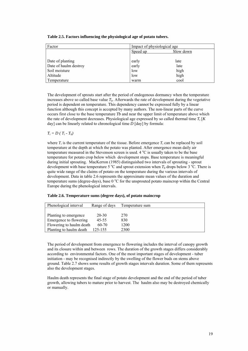
Table 2.5. Factors influencing the physiological age of potato tubers. Factor Impact of physiological age Date of planting Date of haulm destroy Soil moisture Altitude Temperature

Speed up Slow down early late early late low high low high warm cool

The development of sprouts start after the period of endogenous dormancy when the temperature increases above so called base value Tb. Afterwards the rate of development during the vegetative period is dependent on temperature. This dependency cannot be expressed fully by a linear function although this concept is accepted by many authors. The non-linear parts of the curve occurs first close to the base temperature Tb and near the upper limit of temperature above which the rate of development decreases. Physiological age expressed by so called thermal time Tt [K day] can be linearly related to chronological time D [day] by formula: Tt = D ( Ti - Tb) where Ti is the current temperature of the tissue. Before emergence Ti can be replaced by soil temperature at the depth at which the potato was planted. After emergence mean daily air temperature measured in the Stevenson screen is used. 4 oC is usually taken to be the base temperature for potato crop below which development stops. Base temperature is meaningful during initial sprouting. MacKerron (1985) distinguished two intervals of sprouting - sprout development with base temperature 5 oC and sprout extension when Tb drops below 3 oC. There is quite wide range of the claims of potato on the temperature during the various intervals of development. Data in table 2.6 represents the approximate mean values of the duration and temperature sums (degree-days), base 0 oC for the unsprouted potato maincrop within the Central Europe during the phenological intervals. Table 2.6. Temperature sums (degree days), of potato maincrop Phenological interval Range of days Temperature sum Planting to emergence 20-30 270 Emergence to flowering 45-55 830 Flowering to haulm death 60-70 1200 Planting to haulm death 125-155 2300 The period of development from emergence to flowering includes the interval of canopy growth and its closure within and between rows. The duration of the growth stages differs considerably according to environmental factors. One of the most important stages of development - tuber initiation - may be recognised indirectly by the swelling of the flower buds on stems above ground. Table 2.7 shows some results of growth stages intervals duration. Some of them represents also the development stages. Haulm death represents the final stage of potato development and the end of the period of tuber growth, allowing tubers to mature prior to harvest. The haulm also may be destroyed chemically or manually.

20

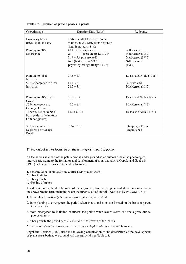
Table 2.7. Duration of growth phases in potato Growth stages Duration/Date (Days) Reference Dormancy break Earlies: end October/November (seed tubers in store) Maincrop: end December/February (later if stored at 4 °C) Planting to 50 % 40 ± 12.5 (unsprouted) Jefferies and Emergence 25 (sprouted)51.9 ± 9.9 MacKerron (1987) 51.9 ± 9.9 (unsprouted) MacKerron (1985) 26.6 (first early at 600 °d Gillison et al. physiological age.Range 25-28) (1987) Planting to tuber 59.3 ± 5.4 Evans, and Nield (1981) Initiation 50 % emergence to tuber 17 ± 3.3 Jelferies and Initiation 21.5 ± 3.4 MacKerron (1987) Planting to 50 % leaf 56.8 ± 5.4 Evans and Nield (1981) Cover 50 % emergence to 40.7 ± 6.4 MacKerron (1985) Canopy closure Tuber initiation to 50 % 112.5 ± 12.5 Evans and Nield (1981) Foliage death (=duration Of tuber growth) 50 % emergence to 104 ± 11.9 Dunjasky (1995) Beginning of foliage unpublished Death Phenological scales focussed on the underground part of potato As the harvestable part of the potato crop is under ground some authors define the phenological intervals according to the formation and development of roots and tubers. Gupalo and Gončarik (1971) define four stages of tuber development: 1. differentiation of stolons from axillar buds of main stem 2. tuber initiation 3. tuber growth 4. ripening of tubers

The description of the development of underground plant parts supplemented with information on the above ground part, including when the tuber is out of the soil, was used by Polevoy(1983):

1. from tuber formation (after harvest) to its planting in the field

2. from planting to emergence, the period when shoots and roots are formed on the basis of parent tuber reserves

3. from emergence to initiation of tubers, the period when leaves stems and roots grow due to photosynthesis

4. tuber growth, the period partially including the growth of the leaves

5. the period when the above-ground part dies and hydrocarbons are stored in tubers

Engel and Raeuber (1962) used the following combination of the description of the development of plants parts both above-ground and underground, see Table 2.8:

21

Table 2.8 Phenological phases of the potato according to Engel and Raeuber (1962). Phenological term used Phenological phase 0. Germination From seeding to emergency 1A. Youth A From emergency to beginning of stolon formation 1B. Youth B From stolon formation to beginning of tubers formation 2. Tubers formation From beginning of tubers formation to the beginning of flowering 3. Flowering From the beginning to the end of flowering 4. Ripening From the end of flowering to berry maturity 5. Old age From berry maturity to full haulm dead

Phenological scales focussed on the above-ground part of potato

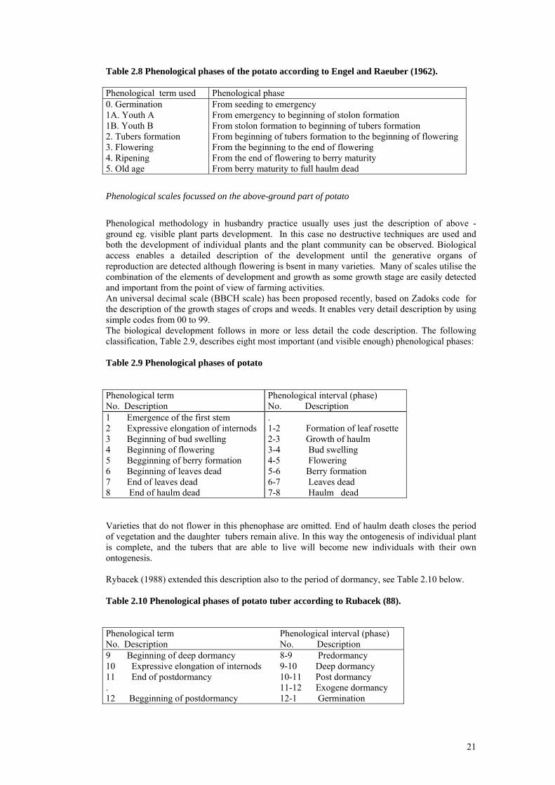
Phenological methodology in husbandry practice usually uses just the description of above - ground eg. visible plant parts development. In this case no destructive techniques are used and both the development of individual plants and the plant community can be observed. Biological access enables a detailed description of the development until the generative organs of reproduction are detected although flowering is bsent in many varieties. Many of scales utilise the combination of the elements of development and growth as some growth stage are easily detected and important from the point of view of farming activities. An universal decimal scale (BBCH scale) has been proposed recently, based on Zadoks code for the description of the growth stages of crops and weeds. It enables very detail description by using simple codes from 00 to 99. The biological development follows in more or less detail the code description. The following classification, Table 2.9, describes eight most important (and visible enough) phenological phases: Table 2.9 Phenological phases of potato Phenological term No. Description

Phenological interval (phase) No. Description

1 Emergence of the first stem . 2 Expressive elongation of internods 1-2 Formation of leaf rosette 3 Beginning of bud swelling 2-3 Growth of haulm 4 Beginning of flowering 3-4 Bud swelling 5 Begginning of berry formation 4-5 Flowering 6 Beginning of leaves dead 5-6 Berry formation 7 End of leaves dead 6-7 Leaves dead 8 End of haulm dead 7-8 Haulm dead

Varieties that do not flower in this phenophase are omitted. End of haulm death closes the period of vegetation and the daughter tubers remain alive. In this way the ontogenesis of individual plant is complete, and the tubers that are able to live will become new individuals with their own ontogenesis. Rybacek (1988) extended this description also to the period of dormancy, see Table 2.10 below. Table 2.10 Phenological phases of potato tuber according to Rubacek (88). Phenological term No. Description

Phenological interval (phase) No. Description

9 Beginning of deep dormancy 8-9 Predormancy 10 Expressive elongation of internods 9-10 Deep dormancy 11 End of postdormancy 10-11 Post dormancy . 11-12 Exogene dormancy 12 Begginning of postdormancy 12-1 Germination

22

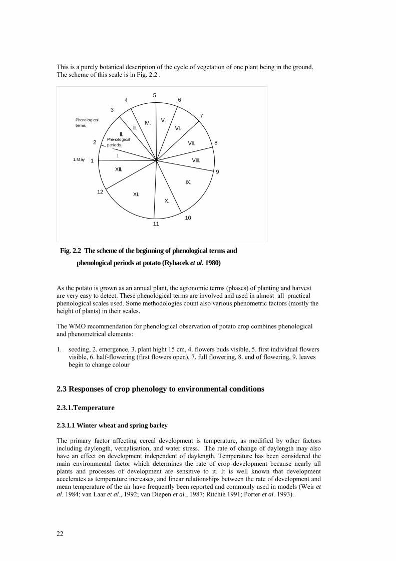
This is a purely botanical description of the cycle of vegetation of one plant being in the ground. The scheme of this scale is in Fig. 2.2 .

III.II.

I.

XII.

XI.X.

IX.

VIII.

VII.

VI.V.IV.

Phenologicalperiods

1. M ay

Phenologicalterms

1

2

3

45

6

7

8

9

1011

12

Fig. 2.2 The scheme of the beginning of phenological terms and

phenological periods at potato (Rybacek et al. 1980) As the potato is grown as an annual plant, the agronomic terms (phases) of planting and harvest are very easy to detect. These phenological terms are involved and used in almost all practical phenological scales used. Some methodologies count also various phenometric factors (mostly the height of plants) in their scales. The WMO recommendation for phenological observation of potato crop combines phenological and phenometrical elements: 1. seeding, 2. emergence, 3. plant hight 15 cm, 4. flowers buds visible, 5. first individual flowers

visible, 6. half-flowering (first flowers open), 7. full flowering, 8. end of flowering, 9. leaves begin to change colour

2.3 Responses of crop phenology to environmental conditions

2.3.1.Temperature 2.3.1.1 Winter wheat and spring barley The primary factor affecting cereal development is temperature, as modified by other factors including daylength, vernalisation, and water stress. The rate of change of daylength may also have an effect on development independent of daylength. Temperature has been considered the main environmental factor which determines the rate of crop development because nearly all plants and processes of development are sensitive to it. It is well known that development accelerates as temperature increases, and linear relationships between the rate of development and mean temperature of the air have frequently been reported and commonly used in models (Weir et al. 1984; van Laar et al., 1992; van Diepen et al., 1987; Ritchie 1991; Porter et al. 1993).

23

Modellers have attempted to assess quantitatively the effects of temperature by calculating accumulated thermal time. As shown before, relationships have been found to vary in form from simple linear to variously non linear forms but they are generally limited and specific to site and plant material. This can be expected since most relationships are descriptive rather than based on underlying processes. Phenological development begins with germination of the seed and the emergence of the seedling through the soil surface. In this phase, the soil environment is more important than the aerial environment. Thermal time is generally based on air temperature but during early growth, when meristems are still below or near the ground, it may be most appropriate to use soil temperature to accumulate thermal time. The time to emergence of the coleoptile from the soil varies with the sowing date, mainly due to temperature differences and soil water status. When sowing are made in warm soil in early autumn, for example, seedlings may emerge in about 5 days, but in November, emergence may take several weeks. The response of seedling emergence to temperature is approximately linear. The point of intersection of the response line with the temperature axis indicates the minimum temperature for germination. Because of the linear nature of the response, it is possible to use thermal time to analyse and predict seedling emergence. The number of degree days from sowing to emergence varies from about 70 to 200 degree-days with a base temperature which varies around 1 °C. Increasing the depth of sowing increases the time taken for seedling emergence. In terms of accumulated temperature units, each extra centimetre that the seed is buried increases the time to seedling emergence by about 10 degree-days (Ritchie, 1991). There is no single relationship between rate of development from emergence to double ridge phase. Experiments conducted in England to measure the variation in development of winter wheat (Porter et al , 1987), has shown that there is a good linear relation between the rate of development and photothermal units calculated for a base temperature of 0 °C. For the following phases the authors found that there was a satisfactory relationship between the rate of development and mean temperature with an increasing base temperature for later phases of the development cycle. It was about 2 °C for the double ridges to the terminal spikelet phase, 3.5 °C for double spikelet to anthesis and 6 °C during grain filling. In one respect, this last phase is the simplest one to analyse because temperature appears to be the major factor affecting its duration. Genotypes vary significantly in their degree of sensitivity to temperature, but there is not necessarily an association between this sensitivity and the duration of the period to a specific development stage. The basic development rate is not only a genotypic characteristic but a result of the interaction between the genotype and the thermal environment. The effect of the vernalisation factor discussed later in this section can explain the modification of the ranking of genotypes for their development rates which is sometimes observed when temperature is changed. The literature indicates that, the durations of different phenophases are independent of each other, thus implying that the duration of any phase of development could be modified without compensatory changes occurring in the duration of other phases. If different phenophases are independent, they may also differ in their sensitivity to the environment.

The response of phasic development for winter wheat to temperature as well as to photoperiod, vernalisation and water are summarised in Table 2.8. The total life cycle is divided into the most commonly used stages to describe development of winter wheat . The importance of the effect of each is marked by different signs: (+++), strong effect; (++), moderate or variable effect due for example to genotype; (+) slight effect not clearly demonstrated in literature; (-), no known effect. As can been seen, there is no phase during which temperature does not modify development

24

Table 2.8. Environmental factors affecting crop development

Developmental phase

Temperature

Photoperiod

Vernalisation

Water stress

Sowing to emergence Emergence to floral initiation Floral initiation to terminal spikelet Terminal spikelet to heading Heading to anthesis Anthesis to maturity

+++ +++ ++

+++ +++ +++

-

++ +++ ++ - -

-

+++ ++ + - -

++ + + + +

++

2.3.1.2 Potato Temperature represents the most important constituent of the environment affecting both development and growth of potato crops. Temperature limits determine the possible range below/above which the potato plant does not grow and even dies. Between these limits the temperature determines the rate of growth and development. The development of the potato starts in the underground and so soil temperature at10 cm depth is a meaningful factor during the first phase of development. The relationship between the potato growth and temperature varies during the period of vegetation and as shown before, even the base temperature during the first phenological phase after planting is not constant. Though many mathematical expressions describing potato growth and development according to the temperature were found, the method of temperature sum with the assumption of linear relationship is widely used in the models.

The Chlilean centre of the European potato has a maritime climate with a high precipitation and relatively high air humidity. The daily temperature amplitude is relatively low, but the length of the day is longer than in the tropics. The day and night temperatures especially during the month of July are lower than in Europe.

European varieties of potato belong to the crops of temperate zone. The most favourable condition is the coastal climate with a higher air humidity. As for the inland areas this condition is fulfilled mostly at higher altitudes. The greatest difference from optimal climate requirements can be expected by growing very early varieties. They are grown mostly at the lowest and so relatively warm regions. These situations usually require irrigation. The highest yields from non-irrigated crops in the areas inland were obtained at heighths around 500 m a.s.l. But there are many differences associated with regional scale across Europe.

Air temperature is the crucial factor for tuber germination. Intervals of 15-20oC is considered to be the optimum for this process. Temperature change accelerates the process of germination more or less quick. Haulm growth starts at 5-6oC and the optimum growth is around 17-25 oC. The most intensive photosyntheses occurs during the period of haulm development.so that the temperature at this stage has marked influence on the final yields; clearly optimal temperature is highly desirable at this stage. At 30oC haulm growth stops. Temperature over 40oC injures the tissue above ground. Potato haulm has relatively poor resistance to low temperature. Periods when the air temperatures of from -1 to -1,5oC persists long enough can cause haulm death from freezing. Tubers freeze, according to the variety, from -1 to -2,2°C. This risk is expected in very early varieties during late spring frosts.

Tubers grow most rapidly at temperatures around 17oC with a range for their development of 2 - 29 oC. At air temperature over 45 oC the tubers die. Soil temperature plays a decisive role in potato plant development. Soil temperature increases firstly by intercepted radiation and after canopy closure mostly by the exchange of atmosphere and soil air. An aerated soil can warm more rapidly. Soils with a high water content warms relatively

25

slowly. Soil temperature during the period of vegetative growth should be lower than air temperature, 15-17oC is the optimum; at a soil temperature of 26 oC the growth of tubers ceases. Temperature also influences the period of dormancy. It is possible to distinguish easily the periods of endogenous and exogenous dormancy. The intensity of metabolism in this cryptovegetative stage can be expressed by the rate of respiration. This process is highly dependent on the temperature range.(See fig. 2.2 ).

0

1

2

3

4

5

6

7

8

XI XII I II III IV V VI month

mgCO

2.kg.h

-1

1oC5oC15oC

Fig.2.2 The speed of breathing at various temperatures.. (Hruska et al., 1974)

Temperature regimes schedule the time of planting and consequently the length of the whole period of vegetation. For each variety and planned harvesting date there is a correct physiological age and required planting date which will lead to optimal development and yields. For the early varieties the optimum ages for the early harvesting period differs according to the accumulated storage temperature. As the growth of tubers is determined by the development of above ground plant parts the correct physiological age under the certain temperature conditions can become the limiting factor for yield. The effect of temperature on the total tuber yield in maincrop varieties is demonstrated in fig. 2.2.

2.3.2 Photoperiod 2.3.2.1 Winter wheat and spring barley The photoperiod stimulus for crops is perceived by the leaves and a signal transmitted to the apex. Consequently cereal plants cannot respond to photoperiod before the crop emerges. Photoperiod at crop emergence has been shown to affect the rate of leaf initiation and this clearly has an effect on the date when reproductive development starts. Wheat and barley are quantitative long-day plants and it is well known that the development is faster during long days. It is usually considered that photoperiod primarily affects the rate of development in the early stages of cereal growth as shown by Porter and Delecolle (1988) for wheat. The most critical sensitivity for cereal crops is during the interval from seedling emergence to floral initiation. Duration of this interval determines total number of leaves initiated and thus the number which must emerge prior to flower appearance. As plants move closer to the flowering stage, it appears that the influence of this is reduced.

26

The rate of leaf emergence increases as sowing date for winter wheat is delayed from September towards the end of the year. The number of leaves on the main shoot generally varies from about 10 to 15. Exposure to low temperatures and long days in the early stages of plant development tends to reduce the number of leaves per shoot (Kirby, Appleyard and Fellowes, 1985). While photoperiod is reported to affect the rate of leaf emergence, it does not explain differences in field observations. Identification of interactions between daylength response and temperature response in the field are difficult because of the seasonal trends of both environmental variables. As daylength increases in the spring, temperature also increases. Simple descriptions of daylength responses in terms of days have led to numerous contradictory reports. The daylength response also appears to differ among genotypes. For winter wheat the response to photoperiodis is approximately linear with a base photoperiod of about 7 hours for emergence to anthesis (Weir et al, 1984). These authors have also shown that there were no significant effects of photoperiod on the duration of the grain filling phase. 2.3.2.2 Potato

Photosynthetically active radiation, often expressed as the daylight, is the decisive part of the environment influencing the development of the crop.The response of the crop to daylight that defines the photoperiod starts more or less after the crop emerges. Because potato is grown in Europe under various environmental conditions the influence of photoperiod on the process of assimilation may vary considerably.

Potato species of Andean origin potato are short-day plants. In Europe potato species had to adapt to longer daylengths - and so the varieties grown in the Europe are mostly long-day reactive or photoperiod neutral.

The potato plant has requirement for light changes during the vegetative period. At the pre-germination stage the short, eight hour day encourages the growth of buds. Long days over 14 hours inhibits or reduce this process. The minimum intensity of illumination should be 800 lux. The long day with 15 and more hours of light favour the growth of haulm of all species. Flowering starts sooner under long day conditions - but except for the period from emergence to the bud swelling all phenological intervals become longer. This extends the period of vegetative growth. New tubers start to grow later but finally they are bigger and also the content of starch is higher. The influence of illumination on tuber growth can be eliminated by temperature. Below 14oC there is no influence of day-length on tuber formation. So at low temperature tuber formation is driven by temperature, at higher temperature by day-length. Varieties differ considerably in their response to varying photoperiods (see fig. 2.3).

The proportion of intercepted radiation increases with the total area of the green leaves and stems. As the photosyntetically active radiation is the catalyst for the assimilation process, a high rate of assimilation can be achieved by a rapid development of a favourable leaf area index. Potato crops intercept arround 80 % of radiation at a leaf area index near 4. So reaching a leaf area index approximatly 4 as rapidly as possible should lead to the highest yields. However, very early development of potato canopy with adequate leaf area index in relatively short time is usually associated with early senescence and the cycle of vegetative growth is shorter.

27

0

100

200

300

400

500

600

700

from emergencyto first buds

beginning of flowering

bud swelling

end of flowerinfg

drying up

dry haulm

very early early half early half late late

24 D 8 24 D 8 24 D 8 24 D 8 24 D 8

Fig. 2.3 The influence of daylight on the development of various variety of potato. (Hruska et all 24-24 hours visible light, D - natural visible light, 8 - 8 hours visible light )

The photoperiod and the temperature exert major influences on the distribution of dry matter. Long days associated with high temperatures reduce the initiation of tubers but promote the development of above-ground parts of the crop. The stimulus for tuberisation is associated with shorter days and relatively low temperatures . There are limits as to the daylength, for each variety, beyond which tuber formation is restricted. In varieties with a long period of vegetative growth the process of tuber formation is more affected by daylength than in early varieties with a shorter period of vegetative growth.

2.3.3. Vernalisation 2.3.3.1 Cereals Crops that flower after a period of relatively cold weather, such as winter grains, usually have a vernalization requirement, i.e., a period of several weeks of near frost, that must be met before rapid development toward flowering can begin. Without vernalisation, flowering of winter grains is delayed. Vernalisation of cereals is accomplished by the exposure of the plants, or the imbibed seeds, to temperatures between 0°C and 12°C for a period of weeks depending on the actual temperatures and the cultivar. The effect of this vernalisation is to reduce the number of leaves initiated and to promote earlier floral development. Vernalisation does not affect the time taken from sowing to crop emergence or from anthesis to maturity but only the duration of phases between crop emergence and anthesis. It is generally recognised that exposure to vernalising temperatures after seed imbibition has an influence on the rate of development of wheat during the vegetative stages. Its influence is not well established for the time from floral initiation to anthesis. There is also a considerable genotypic variation in the

28

response to vernalisation in the durations of the phases, emergence to double ridge and double ridge. Nevertheless, the effects are greater in the earlier phase. Vernalisation has been modeled by accumulating vernalisation units during cold periods, when temperatures are situated between 0 °C and 10 °C, and loosing accumulated units during warm periods. The problems to be resolved include determining the minimum, optimum, and maximum temperatures for accumulating and reducing accumulated vernalisation units, the growth stage when accumulation should begin, and the rate functions to be used for accumulation. 2.3.4. Water stress 2.3.4.1.Winter wheat and spring barley The ratio of actual (ET) and potential evapotranspiration (ET0) to potential evaporation (PE) has been used by several authors as a measure of the daily or seasonal crop water use and moisture deficit. The average ET/PE for specific phenological stages has been used as an index to reflect the moisture deficit condition (Doraiswamy & Thompson, 1982). The change in the ratio is influenced by the soil water deficit and the crop development stage. The ratio may be small during the early stages and during senescence when evapotranspiration is relatively small compared to potential evaporation.The difference in ratio ET0 /PE and ET/PE provides the stress index (SI) Daily water stress may be characterized by an index whose value is between 0 and 1 and which is the ratio between actual and potential transpiration of the crop. Relatively little information is available on water stress effects on phenology. The adjustment of crop development to water stress is stage specific. Doraiswamy & Thompson (1982) proposed to multiply the daily increment of crop development functions of the type: a1 e-SI for emergence to heading and a1 + a2 SI + a3 SI2 for the latest phases where a1, a2 and a3 are crop specific coefficients equal to or less than 1. The primary effects of water stress are on growth processes but some phenological processes may also be affected. Mild water stress in the early vegetative stages of the plant tends to slow floral initiation. Maximum evaporative demand occurs around heading and flowering when the leaf canopy is greatest. The energy which cannot be dissipated in latent heat fluxes causes an increase in plant temperature which hastens senescence and a rapid maturation. 2.3.4.2 Potato Potato water requirements vary within a large range according to the variety. The transpiration coefficient (the amount of water in kg necessary for the production of 1 kg of dry matter) for early varieties is 250-280, for late varieties sometimes over 500. This index also depends on soil type.

Potato water requirement ETp can be defined by the general expression:

ETp = kc ET0

where Et0 is potential evapotranspiration, kc is a crop coefficient that expresses the rate of transpiration in well-watered potato crops compared to grass. It varies according to the stage of development and the state of the atmosphere. From the attainment of effective full groundcover it reaches 1.05 to 1.2 (Doorenbos and Pruit, 1977). Jørgensen (1984) defined water stress Ds for a number of days as a ratio of actual Ea and potential evaporation Ep :

Ds = (1 - Ea/Ep) d

where d is the number of days.

The potato plant is quite sensitive to water supply distribution, and as a vegetatively productive plant it responds to variations in moisture content within the available range of soil moisture (Hukkeri and Moolani, 1965). At germination there is relatively week dependence on water supply. Because water is the major ingredient of potato tuber (over 70 % of the content) during germination the process of growth can be predominantly supplied with water from mother tuber. The periods of tuber development and flowering are much more sensitive. As the potato is a shallow rooted crop, it obtains water mostly from the upper soil layer. Many authors (Gausman,1959; Weawer,1929; Boone at al.,1978) reported maximum concentration of the root

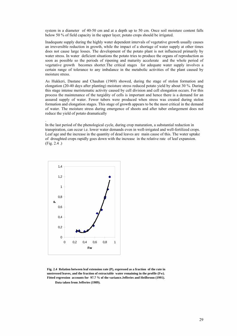
29

system in a diameter of 40-50 cm and at a depth up to 50 cm. Once soil moisture content falls below 50 % of field capacity in the upper layer, potato crops should be irrigated.

Inadequate supply during the highly water dependent intervals of vegetative growth usually causes an irreversible reduction in growth, while the impact of a shortage of water supply at other times does not cause large losses. The development of the potato plant is not influenced primarily by water stress. In water deficient situations the potato tries to produce the organs of reproduction as soon as possible so the periods of ripening and maturity accelerate and the whole period of vegetative growth becomes shorter.The critical stages for adequate water supply involves a certain range of tolerance to any imbalance in the metabolic activities of the plant caused by moisture stress.

As Hukkeri, Dastane and Chauhan (1969) showed, during the stage of stolon formation and elongation (20-40 days after planting) moisture stress reduced potato yield by about 30 %. During this stage intense meristematic activity caused by cell division and cell elongation occurs. For this process the maintenance of the turgidity of cells is important and hence there is a demand for an assured supply of water. Fewer tubers were produced when stress was created during stolon formation and elongation stages. This stage of growth appears to be the most critical in the demand of water. The moisture stress during emergence of shoots and after tuber enlargement does not reduce the yield of potato dramatically

. In the last period of the phenological cycle, during crop maturation, a substantial reduction in transpiration, can occur i.e. lower water demands even in well-irrigated and well-fertilized crops. Leaf age and the increase in the quantity of dead leaves are main cause of this. The water uptake of droughted crops rapidly goes down with the increase in the relative rate of leaf expansion. (Fig. 2.4 .)

0

0,2

0,4

0,6

0,8

1

1,2

1,4

0 0,2 0,4 0,6 0,8 1

Fw

P

Fig. 2.4 Relation between leaf extension rate (P), expressed as a fraction of the rate in unstressed leaves, and the fraction of extractable water remaining in the profile (Fw). Fitted regression accounts for 97.7 % of the variance.Jefferies and Heilbronn (1991). Data taken from Jefferies (1989).

30

Several workers established an empirical relationship in order to quantify the effect of water stress on potato yield. Doorenbos and Kassam (1979), in an empirical study, using the relative yield decrease and relative evapotranspiration deficit stated the yield response factor (Ky). It was low during the periods of early vegetative growth (0.45) and ripening (0.2). Tuber initiation and yield formation periods showed Ky to be about 0.8.

2.3.5. Nitrogen stress 2.3.5.1 Cereals The effect of nitrogen shortage on phenological development of winter wheat has also been reported in the literature (Seligman et al. , 1983). Under nitrogen deficient conditions a wheat crop reaches maturity earlier than crops growing in a normal situation. Nitrogen stress causes stomatal closure at higher plant water potentials or a reduction in water supply by an increased root resistance or insufficient development of the root system. As a result transpiration is reduced as with water stress. A delay of 5 days may be observed. It corresponds to a difference of 1°C during the main growth period.

2.3.5.2 Potato The physiological state of the potato crop is strongly influenced by the availability of nitrogen. There is a primary effect of the nitrogen deficit/ nitrogen abundance on the potato growth. The development of the crop is affected somewhat indirectly. The growth and extent of above-ground leaf and stem tissue determines the rate of photosynthesis. If nitrogen is deficient the growth is restricted and the content of chlorophyll in the leaves decreases. Consequently, because the growth of tubers is also restricted and the senescence comes sooner, the period of vegetative growth is also shorter. It is necessary to understand that the availability of nitrogen is strongly related to soil moisture and water availability. Water stress restricts the uptake of nitrogen by the crop. On the other hand a negative impact of nitrogen excess on tuberization (e.g. Sebanek et al., 1983) is also recognised. REFERENCES Agrométéorologie operationelle. Recueil de notices phenologiques. Organisation météorologique mondiale, (1991), Genéve Angus J.F., Cunningham R.B., Moncur M.W., MacKenzie D.H. (1981a).Phasic development in field crops. I. Thermal response in the seedling phase. Field Crops Res. 3, 365-378. Angus J.F., MacKenzie D.H., Morton R., Schafer C.A. (1981b).Phasic development in field crops. II. Thermal and photoperiodic responses of spring wheat. Field Crops Res. 4, 269-283. Brown, D. M. (1978) Heat unit for corn in Southern Ontario. Ontario Ministry og Agriculture and Food, Factsheet n0 78.063, 4p Danert, S. (1971) Pflanzenreich in drei banden. Hohere pflantzen 1, Leipzig – Jena – Berlin, Urania Verlag. Danert, S. (1973) Pflanzenreich in drei banden. Hohere pflantzen 2, Leipzig – Jena – Berlin, Urania Verlag. Diepen C. A. Van, Wolf J., van Keulen H. Rappholdt (1989) WOFOST: A simulation model for crop production. Soil use management 5:16-24 Doraiswamy P.C., Thompson D.R. (1982) A crop moisture stress index for large areas and its application in the prediction of spring wheat phenology. Agric. Forest Meteorol. 27, 1-15.

31

Doorenbos, L., Kassam, A. H. (1979) Yield response to water, FAO Irrigation and Drainage Paper, No.33, Rome. Doorenbos, L., Pruit, W.O. (1977) Guidelines for predicting crop water requirements, FAO Irrigation and Drainage Paper, No.24, Rome. Dunajasky, E. (1995) Duration of the phenological phases of potato, (Unpublished) Durand R., Bonhomme R., Derieux M. (1982) Seuil optimal des sommes de températures. Application au maïs (Zea mays L.). Agronomie 2, 7, 589-597. Evans, S. A., Nield, J. R. A. (1981) The achievment of very high yields of potatoes in the U.K., Journal of Agricultural Science, Cambridge, 97, 391-396 Franquin P. (1976) Formulation des phénoménes apparents de photopériodisme en conditions naturelles. Des modéles progressifs. Physiol. Vég. 14,1, 179-191. Gillkinson, T. C., Jenkins, P. D., Hayes, J. D. (1987) Some factors affecting the extension of the physiological age of potato seed tubers, Journal of Agricultural Science, Cambridge, 108, 437-451. Gupalo, P. V. (1966) The growth and development of potato crop, Moskva. (in Russian). Hruska, L. et al (1974) Potatoes, Praha (In Czech) Hukkeri, S.B., Dastane, N. G., Chauhan, D. S. (1969) Effect of soil moisture stress at different stages of growth on the yield of potato. Indian Journal of Agric. Science, 40: 318-327 Hukkeri, S. B., Moolani, M. K. (1965) The effect of levels of fertilization and irrigation on the yield of potato.( Solanum tuberosum L.) Science and Cultivation, 31. Jefferies, R. A., MacKerron, D. K. L. (1987) Thermal time as a non-destructive method of estimating tuber initiation in potatoes, Journal of Agricultural Science, Cambridge, 108. Jørgensen, V. (1984) The effect of water stress on potato growth, development, yield and quality, Tidsskr. Planteavlsforsøg, 88, 453-469. Kirby E.J.M. (1974) Ear development in spring wheat. J. Agric. Sci., Camb. 82, 437-447. Kirby E.J.M., Appleyard M. (1984) Cereal Development Guide. 2nd Edn. (Arable Unit, National Agricultural Centre : Coventry). Kirby E.J.M., Appleyard M., Fellowes G. (1982) Effect of sowing date on the temperature response of leaf emergence and leaf size in barley. Plant, Cell and Environment 5, 477-484. Kirby E.J.M., Appleyard M., Fellowes G. (1985) Variation in development of wheat and barley in response to sowing date and variety. J. Agric. Sci. 104, 383-396. MacKerron, D.K.L. (1984) Potato sprout emergence in soil as a function of temperature and time from planting. European Association of Potato Research, Abstracts 9th Triennial Congress, 4364-5. MacKerron, D.K.L. , Waister, P.D. (1985) A simple model of potato growth and yield, Part I, Agricultural and Forest Meteorology, Volume 34, No 2-.3, p 241-252. MacKerron, D.K.L. (1985) A simple model of potato growth and yield, Part II, Agricultural and Forest Meteorology, Volume 35, , p 285-300. MacKerron, D.K.L. (1992) Agrometeorological aspects of forecasting yields of potato within E.C., Commission of the European Communities, Brussels- Luxembourg.

32

O’Brian, P. J., Allen, E. J., Bean, J. N., Griffith, R. L., Jones, J. L. (1983) Accumulated day-degrees as measure of physiological age and the relationships with growth and yield in early potato varieties, Journal of Agricultural Science, Cambridge, 101 : 613-631. Polevoy, A. N. (1983) Dynamic model of potato yield formation, Meteorology and Hydrology, Gidrometeoizdat, Leningrad, p 79-85. Polevoy, A. N. (1988) The effects of meteorological factors on potato crop growth, development and production, Acta Hortoculturae nb. 214, Agrometeorology of Potato Crop, Wageningen. Rybácek, V. et al (1988) Potatoes, Brambory, Praha, (in Czech). Porter J.R., Delecolle R. (1988) Interaction of temperature with other environmental factors in controlling the development of plants. In : S.P. Long and F.I. Woodward (eds.), Plants and Temperature. Symposia of the Society for Experimental Biology Number XXXXII (The Company of Biologists Limited : Cambridge), 133-156. Porter J.R., Jamieson P.D., Wilson D.R. (1993) Comparison of the wheat simulation models AFRCWHEAT2, CERES-Wheat and SWHEAT for non-limiting conditions of crop growth. Field Crops Res. 33, 131-157. Ritchie J.T. (1991) Wheat phasic development. In : J. Hanks and J.T. Ritchie (eds.), Modelling plant and Soil Systems. Agronomy Monograph n°31, American Society of Agronomy, Madison, WI, 31-54. Robertson G.W. (1968) A biometeorological time scale for cereal crop involving day and night temperatures and photoperiod. Int. J. Biometeor. 12, 3, 191-223. Russel, G. (1990) Barley knowledge base, in the series ‘ An agricultutrsal information system for the European community’, Joint research centre, European Commission, Italy Salaman, R. N. (1949) The history and social influence of the potato, Cambridge Seligman N. G., Loomis R. S., Bruke J. And Abshahi A. (1983) Nitrogen nutritition and phenological development and field grown wheat. Journal Of Agriculural Science 101, 691-697 Sebanek, J., et al (1983) Plant physiology. Praha (In Czech). Thompson W.J., Stokes D.T. (1985) Cereal apex development stages in relation to crop management. Aspects of trial biology 10, Field trial methods and data handling, 415-429. Uherecky, I., belan, F. (1976) Soil temperature effect on duration of some essential growth stages in selected potato varieties. Acta University of Agriculture. Brno. Van Laar H.H., Goudriaan J. And Van Keulen H. (eds) (1992) Simulation of crop growth for potential and water-limited production situations. Simulation Report. CABO-TT, 27, CABO-DLO, Wageningen, 105 p. Vavilov, N. I. (1960) Collected papers in 5 parts. Problems of selection. Task of Euroasia and New World in the origin of cultural plants. Moskva- Leningrad, Akademia Nauk USSR. (In Russian) Weir A.H., Bragg P.L., Porter J.R., Rayner J.H. (1984) A winter wheat crop simulation model without water or nutrient limitations. J. Agric. Sci., Camb. 102, 371-382. Zadoks J.C., Chang T.T., Konzak C.F. (1974) A decimal code for the growth stages of cereals. Eucarpia Bull. 7, 42-52.

33

3. PESTS AND DISEASES

3.1 Influence of environmental conditions on plant pests

3.1.1 Introduction Weather conditions strongly affect three processes of importance for the population dynamics of insect pests: (1) Reproduction: Temperature largely determines insect development rate and, hence, the timing of events such as adult emergence and oviposition with the susceptible growth stages of the crop. Furthermore, unfavourable weather during these stages will reduce the potential of females to lay their full complement of eggs. (2) Mortality: Adverse weather conditions can cause direct mortality. Weather may also influence mortality indirectly by affecting natural enemies and host plant quality. (3) Dispersal: Insects migrate mainly by flight, and weather conditions affect both their willingness to take-off and the distances they travel once air-borne. Most insects pass through certain life stages during their development. The life cycle of holometabolous insects consists of four stages; egg, larva, pupa and adult. Hemimetabolous insects have only three stages; egg, larva and adult. The effect of weather on the insect depends on the development stage. For example, an insect in the life stage adapted to overwintering can tolerate temperatures well below zero, whereas other stages may be killed if exposed to low temperatures for a long time.

3.1.2 Temperature The development rate of insects is directly regulated by temperature. Two types of models are used to forecast insect phenology. Most common are degree-day models, in which the development rate is assumed to increase linearly with temperatures above a certain base. This assumption is valid only within a limited temperature range; development rates decrease at very high temperatures and approaches zero asymptotically at low temperatures. Several non-linear models have therefore been developed to describe temperature effects in a more realistic way. However, for forecasting purposes linear models are more practical since less detailed temperature data is needed; adequate degree-day estimates can be calculated from daily minimum and maximum temperatures. Moreover, predictions based on linear models are often as accurate as those based on more complicated models (Worner, 1992) . The density of temperature measurements needed in forecasting models depends on the mobility of the insect, the occurrence of insects with a high migratory tendency can be predicted from one or a few meteorological stations in a region, whereas site specific data may be needed to model outbreaks of stationary insects. The geographical distribution of insect species is delimited by climate and insects are more or less adapted to the prevailing climate in the regions where they live. Large deviations from normal temperature conditions may therefore cause mortality. Over wintering is often a critical phase in the life cycle of insects living in temperate climates. Unusually cold winters may cause mortality, especially of insect populations living in the margins of their areas of distribution. Conversely, warm winters in northern Europe may increase mortality due to frequent fluctuations between thawing and freezing or by favouring the development of entomophagous fungi. Insect behaviour is highly influenced by temperature. Insects will not take-off for migrational flight unless a certain daily maximum temperature is exceeded. Temperatures thus affect the timing of migration both by regulating the rate of insect development by influencing flight behaviour. Similarly, activities such as feeding and oviposition cease if temperatures are below certain thresholds. The rate of these activities tends to increase with temperature up to a certain limit. Hence, high temperatures during the susceptible stages of a crop often increase infestation rates. Very high temperatures may also negatively influence insect activity and eventually cause mortality, but this is less common since insects are often capable of avoiding extremely high temperatures.

34

Solar radiation modifies the influence of temperature. Certain insect species may increase their body temperature by sun-basking. Moreover, difference in sun exposure among different habitats in a region is a source of variation in the development rate of an insect population.

3.1.3 Precipitation and moisture Individual insects can, within certain limits, tolerate fluctuations in moisture. Their ability to move around and to some extent choose where to live and feed makes them less sensitive to different levels of humidity. This applies also to their rate of development which is more influenced by temperature than moisture. The effects of moisture are more like that of a threshold that has to be passed before a new phase in the insects life can start. One example is the occurrence of adult wheat blossom midges (Contarinia tritici, Sitodiplosis mosellana) in wheat fields. In this case a certain level of soil humidity is a prerequisite for the insect to leave its cocoons and start moving up through the soil and pupate near the soil surface. The timing of adult occurrence in the field is then determined by the temperature following the pupation. (Kurppa, 1989). Precipitation and moisture can be of great importance for populations build up. There are both direct and indirect effects of rain and moisture on mortality. A direct effect is heavy showers of rain that can interrupt the build-up of a population. Rain can dislodge insects (eggs, larvae or adults) from a plant making them fall to the ground. The insects might get killed by natural enemies on the ground and they will have to look for a new feeding site. One indirect effect is that different levels of moisture favours different organism species. Fungi are a group of natural enemies to insects that, mostly, are favoured by humidity. Drought stress makes plants more susceptible to insect attacks. In a period of drought nearly all plant processes are affected (Mattson & Haack, 1987) . These changes in the plant have effects on both insect behaviour and physiological processes. Examples of effects on the plant are changes in growth, nutrient content, content of secondary metabolites, leaf texture, leaf colour, and plant temperature. Furthermore, the amount of tissue available to the insects is reduced. When a pest migrates into a drought stressed crop, the result will be more individuals per plant unit.

3.1.4 Wind Life cycles of insect pests often contain a migratory phase. This is their way of spreading into new habitats or from a summer to a winter host. Apart from the migratory movement they also move in a more trivial way when moving between feeding sites. The movement of insects in air can also be separated into active and passive flying. Active flying is controlled by the insect and includes flying against wind, passive flying means taking off and then floating with the wind to wherever it blows. Passive flying is common among small insects, like aphids, and especially during their migratory phase. Active flight may also be called targeted flight. Targeted flight is often used in relation to aphids, which at the end of a period of passive flying have a phase when they try to settle on a suitable host. During targeted flight the aphids navigate with the aid of colours and odours. Passive flying insects are evenly distributed in the air up to high altitudes. Migrating aphids, for instance, can be found alive at altitudes up to one thousand meters (Isard et al., 1990) . For small insects, suction trap catches at 12 m height have been shown to accurately represent population size on a regional scale (Taylor,1977)

3.2 Influence of environmental conditions on plant diseases

3.2.1 The pathogen, the host and the environment For the outbreak of a plant disease epidemic three elements must be present: a pathogen, a host and a favourable environment. The environment has a controlling influence on the incidence and development of plant diseases. Examples of important environmental factors for the development of plant diseases are temperature, moisture and wind. The microclimate inside a crop is influenced by the crop itself but the most important factor in this respect is the weather. The weather also

35

affects both the pathogen and the host plant directly and consequently has a strong influence on the pathogen/host interaction.

3.2.2 Fungal life cycles The life cycles of fungal pathogens vary to a great extent, but there are some basic features which are common to most species. Important steps in the life cycles for all plant pathogenic fungi are infection, mycelial development in or on the host, spore production and spore dispersal.

Infective agents are usually spores, but living mycelium is also capable of initiating disease under appropriate conditions. Spores germinate and penetrate plant surfaces by either direct penetration through cell walls or through openings, like stomata, lenticels or wounds. After infection the pathogen grows as mycelium either on the surface of the plant tissue or inside it. The reproductive capacity for most pathogens is very high and under favourable conditions is often sufficient to infect every susceptible plant in the vicinity. Infective agents, particularly spores produced as a result of sexual reproduction can endure unfavourable conditions of high or low temperatures or drought and can function as means of survival for the fungus.

3.2.3 Effect of temperature Pathogens require certain minimum temperatures in order to infect and grow. The low temperatures of autumn, winter and early spring are often below the minimum required by most pathogens. Therefore infection seldom occurs during this period and even if the pathogen is already established on the host, the disease does not develop or develops very slowly. Pathogens differ in their preference for higher or lower temperatures. Some pathogens prefer somewhat lower temperatures and they cause disease in areas, seasons or years with cooler weather. For example Phytophthora infestans, which causes potato late blight, is most serious in the northern latitudes, while in the subtropics it is serious only during the winter. Other pathogens require higher temperatures to develop and they are more common in warm climates. The effect of temperature on the development of a particular disease after infection depends on the particular host-pathogen combination. The most rapid disease development usually occurs when the temperature is optimum for the development of the pathogen but is above or below the optimum for the development of the host. Thus, for stem rust of wheat, caused by Puccinia graminis, the time required for a disease cycle is 22 days at 5 °C, 15 days at 10 °C and 5 to 6 days at 23 °C. Since the duration of each disease cycle determines the number of cycles and, therefore, the number of new infections in one season, it is clear that the effect of temperature on the disease development may be very marked.

3.2.4 Effect of moisture Moisture may influence disease development in the form of rain, irrigation water, relative humidity and as dew. The occurrence of many diseases in a particular region is closely correlated with the amount and distribution of rainfall. For most fungal diseases the rainfall determines the severity of the disease and also whether the disease will occur at all during a season. Potato late blight and downy mildew of grapes for example are severe only in areas or during years with high rainfall or high relative humidity during the growing season. In fungal diseases moisture affects spore formation and longevity and particularly the germination of the spores which require a film of water covering the tissues in order to germinate. Most fungal pathogens are dependent on the presence or free water on the host or high relative humidity only during germination of the spores and become independent once they can obtain nutrients and water from the host. In many fungi, moisture also affects the liberation of spores which in some cases only can occur in the presence of moisture. Some pathogens must have high relative humidity or free moisture in the environment throughout their development. Though most fungal pathogens require free water in order to infect the host, the spores of powdery mildew, for example Erysiphe graminis, can germinate, penetrate and cause infection even when there is only high relative humidity in the air surrounding the plant. In powdery mildews, spore germination and infection are actually reduced by the presence of free moisture on the plant

36

surface. In these diseases the severity of disease is limited rather than favoured by wet weather. Thus powdery mildews are more common and more severe in the drier areas of the world and their relative importance decreases as rainfall increases. Moisture in the form of splashing rain drops play an important role in the dispersal of many pathogens both on the same plant and from one plant to another. Dispersal of spores of glume blotch of wheat, caused by Septoria nodorum takes place with difficulty unless there is rainfall sufficient to create splash droplets in which the spores are carried. Moisture in the form of running water can be important in dispersal of pathogens from one field to another. The number of disease cycles per season of many diseases is closely correlated with the amount of rainfall per season, particularly of rainfall that is of sufficient duration to allow establishment of new infections. Leaf wetness duration during the infection process determines if the spores are able to germinate and infect. The minimum leaf wetness period required depends on temperature. Therefore interactions between leaf wetness duration and temperature determine the rate of pathogen establishment and subsequent disease development.

3.2.5 Effect of wind Wind influences plant diseases mainly through its importance in the spread of the pathogen. Most plant diseases that spread rapidly are caused by pathogens that can be spread over long distances by the wind. Some spores are quite delicate and do not survive long-distance transport in the wind while other spores can be transported by the wind for many kilometres. Wind is even more important in disease development when it is accompanied by rain. Wind-blown rain drops can cause spore release from infected tissue and dispersal of spores though the air. Wind can also cause injury on plant surfaces, which facilitate infection by many fungi. Wind might also prevent infection by accelerating the drying of the wet plant surface. The leaf wetness period might then be too short for infection to take place.

3.2.7 Effect of light Solar radiation can be divided into UV radiation, visible light and IR radiation. The photo period, light quality and light intensity have a direct effect on pathogen development. For potato late blight, both spore production and the viability of spores is reduced by light. However, the major effect of solar radiation is its influence on microclimate. The sun dries wet leaves and reduces the humidity in the crop. This results in more unfavourable conditions for sporulation and infection. The intensity of light may also affect the susceptibility of plants or disease severity. This is explained by production of more or less etiolated plants.

References and additional readings Agrios. G. N. 1988. Plant Pathology, 3rd Edition. Academic Press, Inc. Aust. H. J. 1986. Microclimate in relation to epidemics of powdery mildew. Ann. Rev. Phytopathol, 24, 491-510. Isard, S. A., Irwin, M. E. and Hollinger S. E. (1990). Vertical distribution of aphids (Homoptera: Aphididae) in the planetary boundary layer. Environ. Entomol., 19, 1473-1484. Harrison, J.G. (1992). Effects of aerial environment on late blight of potato foliagr – a review. Plant Pathology, 41, 384-416 Kurppa, S. (1989). Wheat blossom midges, Sitodiplosis mosellana (Gehin) and Contarinia tritici (Kirby) in Finland, during 1981-87. Annales Agriculturae Fenniae 28(2): 87-96. Mattson, W. J. and R. A. Haack (1987). The role of drought stress in provoking outbreaks of phytophagous insects. Insect Outbreaks (P. Barbosa and J. C. Schultz), Academic Press, New York.

37

Taylor, L. R. (1977). Aphid forecasting and the Rothamsted insect survey. Journal of the Royal Agricultural Soc. of England, 138, 75-97. Worner, S. P. (1992). Performance of phenological models under variable temperature regimes: consequences of the Kaufmann or rate summation effect. Environ. Entomol., 21, 689-699.

38

4. EFFECTS OF PESTS AND DISEASES ON CROP

4.1. Introduction

Plant diseases and pest infestations result from the interaction of a pathogen/pest with its hosts. This interaction is affected markedly by the environment (temperature, humidity, wind). Hence, any consideration of pests and diseases in crops involves the triangle pathogen/pest - host - environment. There are many different parasitic agents, e g fungi, bacteria, viruses, mycoplasma, nematodes, insects and mites, as well as a few parasitic plants such as dodder (Cuscuta) and witchweed (Striga). The direct and indirect effects of these can cause great yield losses both quantitatively and qualitatively.

4.2. Effects on crop growth The damage on the plant can be caused by direct depletion of inorganic and organic nutrients, or by disturbing the nutrient translocation in the plant. Some pathogens, e. g. the leaf deseases Rhynchosporium secalis and Stagonospora nodorum, mainly reduce yield directly by diminishing the leaf area available for photosynthesis. Other pests and diseases have both a direct and an indirect effect on yield. The grain aphid (Sitobion avenae) causes a yield reduction directly, by sucking phloem sap, and indirectly, by producing honeydew which covers the leaves and reduces photosynthesis. The larvae of the wheat midges (Sitodiplosis mosellana and Contarinia tritici) feeds on kernels, resulting in both yield losses and reduced protein quality. On potatoes there are diseases, e.g. potato late blight (Phytophthora infestans), which cause great yield losses both quantitatively and qualitatively. The reduced leaf area caused by late blight has a major influence on yield level, especially if the pathogen attacks the crop early in its development. Moreover, the leaf disease may lead to tuber blight, which will severely reduce tuber quality. There are also pests, such as colorado beetles (Leptinotarsa decemlineata), that cause yield reductions by the direct destruction of leaf tissue. Other diseases, such as potato virus Y, indirectly influence yield. Different aphid species transmit the virus during the growing season, resulting in progeny tubers infested with potato virus Y. There is only little or no yield reduction due to this infestation. However, when the progeny tubers are used as seed potatoes in the following year the yield will be reduced by approximately 50% compared with using healthy seed potatoes.

4.3 Susceptible phenological stages

The susceptibility of plants changes during the growing season. Examples of factors affecting susceptibility are age resistance, nutrient status and weather conditions. The effects of pests and diseases on crops can be related to certain developmental stages. Some agents have a great influence at early stages which later cause great yield losses. Examples are the fungal diseases.

Bipolaris sorokiniana, barley yellow dwarf virus (BYDV) frit fly (Oscinella frit), bird cherry oat aphids (Rhopalosiphum padi) and powdery mildew (Erysiphe graminis), influence yield at later developmental stages or both at early and later stages. Wheat midges have a great impact on yield during a limited temporal window (flowering), but not at earlier or later stages. The developmental stages at which attacks of various pest and diseases of barley, winter wheat and potato occur, and suitable stages for chemical control, are indicated in Figures 4.1 and 4.2.

39

Barley Wheat F F F F F F F F F F P P P P P P V

GROWTH STAGE*

Erysiphe graminis

Rhynchosporium secalis

Puccina hordei

Bipolaris sorokiniana

Puccina striiformis

Puccina recondita

Pseudocercosporella herpotrichoides

Stagonospora nodorum

Erysiphe graminis

Drechslera tritici-repentis

Sitobion avenae

Metopolophium dirhodum

Rhopalosiphum padi

Sitodipolsis mosellana

Contarinia tritici

Oulema melanopus

Barley yellow dwarf virus

Germination, 0-9 SD Leaf development, 10-19 Tillering, 20-29 Elongation, 30-39 Vegetative growth, 40-49 Budding, 50-59 Flowering, 60-69 Fruit development, 70-79 Fruit ripening, 80-89 Withering, 90-99

* Growth stage according to Zadoks, J. C. et al. 1974

Sensitive stages Control period SD Seed dressing ST Soil treatment

Figure 4.1. Growth stages of cereals in relation to susceptibility to attacks of different pests and diseases.

40

V P P N F F

GROWTH STAGE **

Potato virus Y

Aphididae

Leptinotarsa decemlineata

Globodera spp

Phytophthora infestans

Alternaria solani

Sprouting, 0-9 ST Leaf development, 10-19 Vegetative growth, 40-49 Budding, 50-59 Flowering, 60-69 Fruit development, 70-79 Fruit ripening, 80-89 Withering, 90-99

* Growth stage according Hack, H. et al. 1993.

Sensitive stages Control period SD Seed dressing ST Soil treatment

Figure 4.2. Growth stages of potato in relation to susceptibility to attacks of different pests and diseases

41

5. OVERVIEW OF PHENOLOGICAL MODELS

5.1 Winter wheat and barley

5.1.1 General principles and concepts The objective of this section is to describe the development scale of some models that are available as computer programs. The models discussed are the AFRC Wheat model (Porter et al. 1993) developed in England by the Agricultural and Food Research Council, the CERES Wheat model (Ritchie and Otter, 1985) developed for the International Benchmark Sites Network for Agrotechnology Transfer (IBSNAT) and the Decision Support System for Agrotechnology Transfer (DSSAT), the SUCROS model developed in The Netherlands by van Laar et al. (1992) to simulate crop growth for potential production situations and the WOFOST model also developed in The Netherlands by van Diepen et al in 1989 for incorporation in the Crop Growth Monitoring System (CGMS) for the regions of European Union. These models were developed to simulate the main process of plant and crop growth, the timing of phenological events and the development of the canopy of wheat anywhere it can be grown. The AFRC model is more specifically used in simulating wheat growth and development under European conditions even if it has also been tested in other parts of the world. The CERES model has been evaluated more extensively and adapted to a wide range of environments. All four models operate on a daily time step and require daily weather data. The relationship between these data and crop growth and development models depends on genotype so that parameters of the models have to be adapted to take into account of these variety differences. The models also contain algorithms to reduce potential production in relation to shortage of water and nitrogen but the effects of pests and diseases are not considered even if tentative coupling of pest models to crop models exists in the literature (Teng and Yuen 1990). A detailed description of the AFRC Wheat phenology model is given by Porter (1984) and Weir et al. (1984). The phenological submodel predicts the beginning and ending dates of four phases: sowing to emergence, emergence to double ridge, double ridge to anthesis, and anthesis to maturity. Maturity is chosen to represent the state of the crop at harvest date. Secondary stages have been added to divide these main phases and give a more precise description of development of wheat. They are: floral initiation between emergence and double ridge stages; terminal spikelet and beginning of ear growth between double ridge and anthesis and finally start of grain filling between anthesis and maturity. The CERES-Wheat model contains nine growth phases numbered from 1 to 9. Phases 1 to 6 are the active above-ground development phases delimited by emergence, terminal spikelet, beginning of ear growth, anthesis , beginning of grain fill and finally maturity which ends the cycle. Phase 7 is a fallow or pre-sowing phase which is used to model the soil water balance during the fallow period and to estimate the initial soil water content at sowing. Phases 8 to 9 cover the period from sowing to emergence. The comparison between the two scales is given in table 2.3 of paragraph 2.2.1.2. Both scales are very similar but it appears that the AFRC development sub-model scale is more detailed especially during emergence to the terminal spikelet phase where two additional steps have been included. Progress through growth stages is driven by accumulation of daily thermal time units modified by vernalization and photoperiod factors. Critical and base temperatures are not the same and the temperature driven rate of development varies from phase to phase.

5.1.2 AFRC Wheat phenological submodel The sub-model is given sowing date, site latitude and daily maximum and minimum temperatures. Thermal time is not computed as a simple mean temperature but is a weighted average of eight daily contributions of a cosinusoidal variation between the observed maximum and minimum temperatures. Thermal time is measured as a combination of calendar time, temperature and

42

photoperiod and the calculation procedure differs for each phase. Four types of thermal time are used. For the phase from sowing to emergence, thermal time is calculated using a base temperature of 1°C. From emergence to double ridge, the thermal time is modified by vernalization and photoperiod factors and for the phase from double ridge to anthesis by photoperiod only (at this moment, vernalization is considered to have ended). From anthesis to maturity, thermal time is calculated assuming a base temperature of 9°C. The rate of progress from one stage to the next stage (f) is supposed to be the product of functions of temperature, photoperiod and vernalization: f = g(T) . h(P) . i(V) where T is the temperature, P the photoperiod and V the vernalization factor. If development depends only on temperature then h=i=1. For T > Tb, the function g(T) may be written as: g(T ) = m(T - Tb), where m is the inverse of the thermal time between two stages. The photoperiod effects are based on the number of effective hours calculated for each day. Thermal time is reduced by a factor proportional to the difference between an optimum and a base number of effective hours. The photoperiod factor is also represented by a continuous variable between 0 and 1. The increment of photo-thermal time is obtained by multiplying the temperature function by the photoperiod factor h(P): h(P) = 0 if P< Pb; h(P) = (P - Pb)/(Popt - Pb) if Pb < P < Popt; h(P) = 1 if P > Popt. where Popt is an optimum photoperiod beyond which development is not sensitive to photoperiod (it is set to 20 hours in the model), Pb is set to 0 hours for the phase from emergence to double ridge and 7 hours from double ridge to anthesis. The photoperiod factor is set to 1 during the maturation phase. The state of vernalization is represented as a continuous variable with values ranging between 0 (no vernalization) and 1 (fully vernalized plants ). The vernalization requirements for a specific cultivar is defined by the number of days, in optimal conditions, needed to complete vernalization. The effect of temperature Veff on the vernalization process is given by a temperature-vernalization response curve whose characteristics depend on the sensitivity of plants to vernalization: Veff = 1 if T2 < T < T3; Veff = (T - T1)/(T2 - T1) if T1 < T < T2; Veff = (T4 - T)/(T4 - T3) if T3 < T < T4. Standard values of T1, T2, T3 and T4 are: -4°C, 3°C, 10°C and 17°C. The mean value of Veff is calculated for each day assuming the sinusoidal temperature evolution and the accumulated daily values Vdd since sowing are calculated. The normalised vernalization factor i(V) is defined as: i(V) =0 if Vdd < Vb days; i(V) = (Vdd -Vb)/(Vsat - Vb) if Vb < Vdd < Vsat; i(V) = 1 if Vdd > Vsat. Lumsden (1980) set Vsat at 33 and Vb at 8 vernal days but these values are also variety dependant. In the original version of the AFRC model (Weir et al. 1984), the thermal time at emergence was 148°C days. The duration period between emergence and double ridge was set to 284°C days. It was 600°C days between double ridge and anthesis and 350°C days between anthesis and maturity.

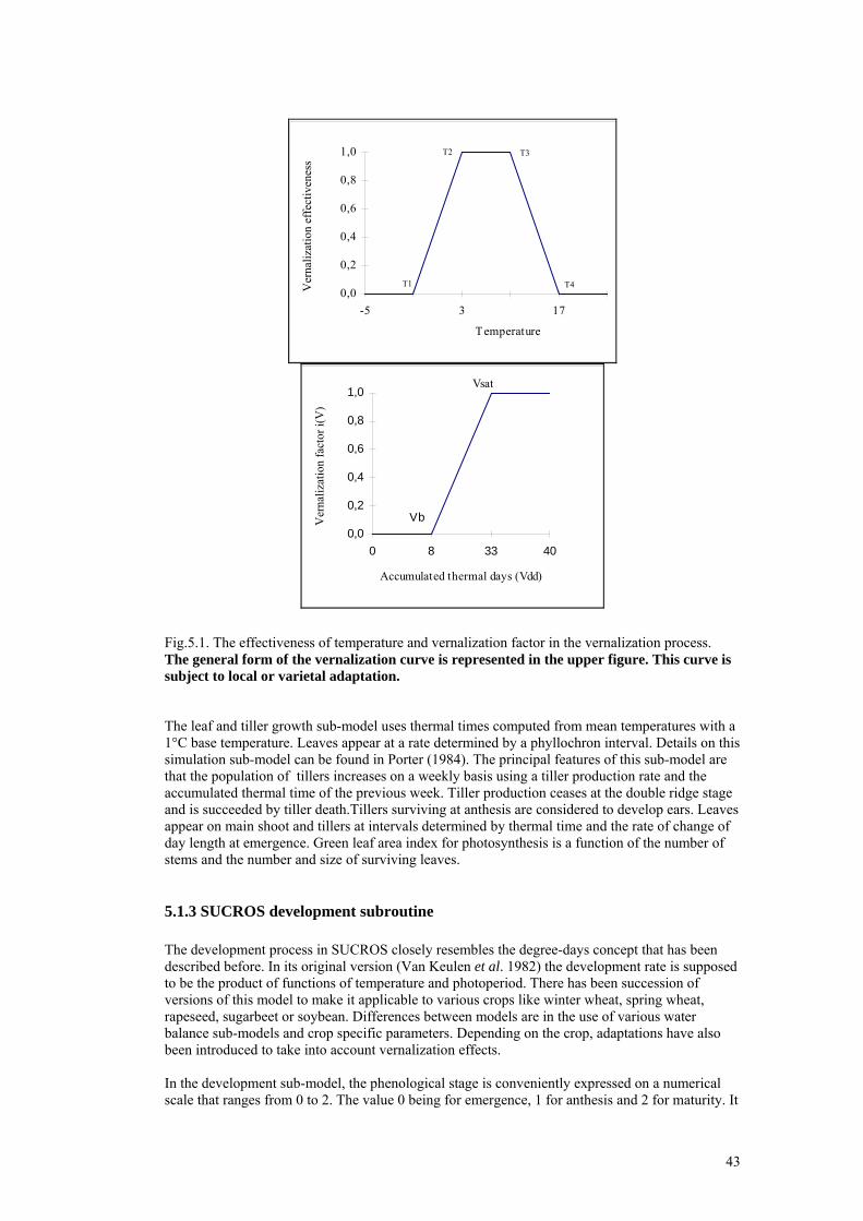
43

T3T2

T4T10,0

0,2

0,4

0,6

0,8

1,0

-5 3 17

Temperature

Ver

naliz

atio

n ef

fect

iven

ess

Vsat

Vb0,0

0,2

0,4

0,6

0,8

1,0

0 8 33 40

Accumulated thermal days (Vdd)

Ver

naliz

atio

n fa

ctor

i(V

)

Fig.5.1. The effectiveness of temperature and vernalization factor in the vernalization process. The general form of the vernalization curve is represented in the upper figure. This curve is subject to local or varietal adaptation. The leaf and tiller growth sub-model uses thermal times computed from mean temperatures with a 1°C base temperature. Leaves appear at a rate determined by a phyllochron interval. Details on this simulation sub-model can be found in Porter (1984). The principal features of this sub-model are that the population of tillers increases on a weekly basis using a tiller production rate and the accumulated thermal time of the previous week. Tiller production ceases at the double ridge stage and is succeeded by tiller death.Tillers surviving at anthesis are considered to develop ears. Leaves appear on main shoot and tillers at intervals determined by thermal time and the rate of change of day length at emergence. Green leaf area index for photosynthesis is a function of the number of stems and the number and size of surviving leaves.

5.1.3 SUCROS development subroutine The development process in SUCROS closely resembles the degree-days concept that has been described before. In its original version (Van Keulen et al. 1982) the development rate is supposed to be the product of functions of temperature and photoperiod. There has been succession of versions of this model to make it applicable to various crops like winter wheat, spring wheat, rapeseed, sugarbeet or soybean. Differences between models are in the use of various water balance sub-models and crop specific parameters. Depending on the crop, adaptations have also been introduced to take into account vernalization effects. In the development sub-model, the phenological stage is conveniently expressed on a numerical scale that ranges from 0 to 2. The value 0 being for emergence, 1 for anthesis and 2 for maturity. It

44

is regarded as a state variable whose value increases with the rate of development which is defined as that part of the scale that is accumulated per day. Intermediate development stages may be obtained by integration of this rate of development until a specific value is reached. The model normally starts at emergence but in recent versions, the day of emergence can be determined by the model itself as a function of the sowing date and the effective daily temperature sum. A linear regression function is used to relate the rate of emergence (dEmerg) to the daily average temperature. dEmerg = 0 if T ≤ 0 dEmerg = m1T if 0 < T < Tb dEmerg = m1Tb + m2(T-Tb) if T ≥Tb where T is the mean air temperature, Tb is a base temperature for emergence, m1 and m2 are regression parameters which are variety dependant. The day of emergence is reached when the integral of the successive dEmerg equals 1. In the simulation of the development of emerged plants, the effective increase in temperature sum used for calculation of development rate is specified in tables taking account of non linearity. The development rate is deduced by a linear interpolation procedure. The shapes of these functions are presented in figure5.2 for the pre-anthesis and the post-anthesis periods. These original functions did not take into account corrections in degree-day summation for high temperatures. New updates of the model (Goudriaan and Van Laar, 1994) have corrected this problem. The ways to calculate the photoperiod and vernalization effects are quite similar to those in the AFRC model. The rate of development is reduced by multiplying the temperature function by a factor ranging between 0 and 1. After anthesis only temperature affects this development rate. For photoperiod, the factor is deduced from a table similar to that for temperature response or is simply proportional to daylength divided by 24.

Pre-anthesis

Post-anthesis

0

0,01

0,02

0,03

0,04

0,05

0 10 15 20 25 30 35

Temperature (°C)

Rat

e of

de

velo

pmen

t

Fig. 5.2. Relationship between development rate and temperature during pre-anthesis and post anthesis stages in the SUCROS model The vernalization rate and the vernalization factor are calculated from complex functions whose general shape is the same as that described in the previous section for the AFRC model. That means that they are also species and variety dependant and that most of the parameters have also to be established experimentally.

5.1.4 WOFOST Crop simulation model WOFOST was originally developed as a crop growth simulation model for the assessment of the yield potential of annual crops in tropical countries but it has been used for the estimation of the regional production potential of the major field crops in the European Community. The WOFOST model describes phenological development of crops from emergence until maturity on the basis of genetic characteristics, temperature and daylength. WOFOST is a product of the family of models

45

developed by the school of Wageningen. It is therefore closely related to the SUCROS model. The development module described here corresponds to version 6.0 of the model (Supit et al. 1994). The development stage is also expressed in a dimensionless variable varying between 0 and 2. The key stages are seedling emergence, flowering and maturity but the sowing date can also be chosen. The daily effective temperature during the germination phase depend on a base temperature below which no physiological activity takes place, and a maximum daily temperature beyond which activity increases no further. Between these two thresholds the effective daily temperature is T - Tb (crops from temperate regions are characterised by a base temperature of 0-3°C). The effective temperatures are summed until some threshold corresponding to emergence is achieved. Development rate before anthesis is controlled by temperature and day length whereas after anthesis only temperature is active. In the model the effective daily temperature (DT) is determined in a table allowing for non linearity. The development rate per day (Dr) is the ratio of this temperature to the temperature sum required to achieve a given stage. It is crop or variety dependant.

D DTTr

i

=∑

The development stage at any step of time is the integral of the development rate. During the vegetative stages a reduction factor (f) ranging between 0 and 1, is introduced to take into account the photosensitivity of the crop. Its value is determined as in AFRC wheat model. The effective development rate is calculated by multiplying the actual development rate by the reduction factor.

5.1.5 Ceres Wheat The phasic development in CERES is organised in growth stages from pre-sowing or sowing to grain maturity. These growth stages are numbered from 1 through 9 (table 9). Stages 1 to 6 are the active above ground stages, stage 7 is used to model the soil water balance during the fallow period and to simulate the soil water conditions at sowing; stage 8 is the sowing to germination period and stage 9 the period from germination to seedling emergence. The progress through the different growth stages is driven by accumulation of thermal time units (DTT) which are eventually modified by vernalization and photoperiod during the emergence to floral initiation period. The daily thermal time units are calculated from observed minimum and maximum air temperatures with a base temperature of 0°C for stages 1 through 4, 1°C for stages 5 through 8 and 2°C for stage 9. When the air temperatures is less than 0°C a correction factor is introduced to take into account the difference between the plant crown and the air temperature. The depth of the snow cover also modifies the crown temperature during freezing periods. It is assumed that development rate is directly proportional to temperature in the range of base temperature to 26°C. Between 26 and 34°C the daily contribution to thermal time is set to a maximum of 26 units. For maximum air temperature greater than 34°C the daily contribution is progressively reduced to reach a value of zero at 60°C. Vernalization is supposed not to occur during stage 9 and 1 for temperature below 0°C or above 15°C or 17°C, the optimum being observed in the range from 0 to 7°C. The minimum and maximum daily temperatures are used to calculate the daily vernalization effectiveness factor (Veff) with a value between 0 and 1. The general shape of the vernalization curve is similar to that described for the ARFC wheat model. Vernalization is complete when Vdd, the sum of the daily Veff, is equal to 50 (Fig.5.3). VF = 1 - P1V*(50 - Vdd)

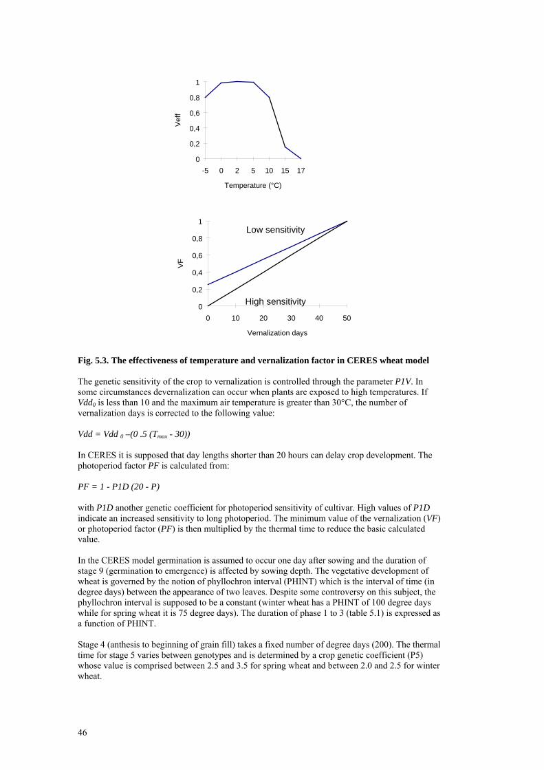
46

0

0,2

0,4

0,6

0,8

1

-5 0 2 5 10 15 17

Temperature (°C)Ve

ff

Low sensitivity

High sensitivity0

0,2

0,4

0,6

0,8

1

0 10 20 30 40 50

Vernalization days

VF

Fig. 5.3. The effectiveness of temperature and vernalization factor in CERES wheat model The genetic sensitivity of the crop to vernalization is controlled through the parameter P1V. In some circumstances devernalization can occur when plants are exposed to high temperatures. If Vdd0 is less than 10 and the maximum air temperature is greater than 30°C, the number of vernalization days is corrected to the following value: Vdd = Vdd 0 –(0 .5 (Tmax - 30)) In CERES it is supposed that day lengths shorter than 20 hours can delay crop development. The photoperiod factor PF is calculated from: PF = 1 - P1D (20 - P) with P1D another genetic coefficient for photoperiod sensitivity of cultivar. High values of P1D indicate an increased sensitivity to long photoperiod. The minimum value of the vernalization (VF) or photoperiod factor (PF) is then multiplied by the thermal time to reduce the basic calculated value. In the CERES model germination is assumed to occur one day after sowing and the duration of stage 9 (germination to emergence) is affected by sowing depth. The vegetative development of wheat is governed by the notion of phyllochron interval (PHINT) which is the interval of time (in degree days) between the appearance of two leaves. Despite some controversy on this subject, the phyllochron interval is supposed to be a constant (winter wheat has a PHINT of 100 degree days while for spring wheat it is 75 degree days). The duration of phase 1 to 3 (table 5.1) is expressed as a function of PHINT. Stage 4 (anthesis to beginning of grain fill) takes a fixed number of degree days (200). The thermal time for stage 5 varies between genotypes and is determined by a crop genetic coefficient (P5) whose value is comprised between 2.5 and 3.5 for spring wheat and between 2.0 and 2.5 for winter wheat.

47

Table 5.1 Development and duration of stages in CERES wheat model

Number

Growth stages

Duration (degree days)

1

2

3

4

5

6

7

8

9

Emergence to floral initiation

Floral initiation to beginning of ear growth

Begin of ear growth to anthesis

Anthesis to beginning of grain fill

Grain filling period

Maturity

Fallow or presowing

Sowing to germination

Germination to emergence

400 PHINT/95

3 PHINT

2 PHINT

200

430 + P5*20

-

-

1 day

40 + 10.2 DEPTH

PHINT, phyllochron interval ; P5, genetic coefficient ; DEPTH, sowing depth in centimetres

5.2. Potato

5.2.1 General principles

The modelling of potato development is always connected with the response of the plant to the environment. Final outputs of such potato crop models deals mostly with pest and diseases and yield prediction. Phenological description of the agrometeorological models of potato is based on the relationship between weather and climate and the crop manifestation parameters though the development and growth is determined by a wider complex of factors. The influence of particular environmental factors on potato growth varies considerably and is very much dependent on variety. The weather analysis and growth simulation models are methodically based on light interception and/or water use. Many models introduce growth curves and crop growth rate for describing the growth process. The date of sowing and emergence are the development stages frequently used in models. After emergence the models work with growth stages rather than development phases. As the interception of solar radiation is the decisive parameter for modelling growth, the expansion of the foliage and finally canopy closure are meaningful parameters for calculating dry matter accumulation by the crop.

Detailed observations of the potato during the vegetative cycle enabled the creation of empirically determined curves that represent crop growth, Following the curve, tuber grading e.g. total dry weight, is determined by environmental parameters. Sands and Regel (1983) assumed the relation of tuber bulking rate and 'phenological time'. The curve for tuber growth was obtained from experimental data, and phenological times for various rates of tuber bulking were empirically derived for Australian conditions. Though the assumption of phenological time based on the bulking rate divides the time of vegetation into phases there is no linkage with the development or growth stage from a phenological point of view.

48

Fig 5.4 Diagrammatic presentation of an approach to analyse the effects of environmental factors on the dry matter production of potato.

5.2.2 A Simple Model of Potato Growth and Yield (England) The model (MacKerron and Waister, 1985) aims to predict the potential yields of potato. Production of total dry matter is calculated as a function of intercepted solar radiation and the partitioning between tops and tubers is based on an empirical study. The development of the crop is divided into three discrete phases: a) from planting to emergence b) from emergence to canopy closure c) from canopy closure to haulm destruction The rate of growth in the model is determined by the response to temperature and solar radiation. The time from planting to emergence is calculated from experimentally derived relationships between temperature and sprout extension rate using soil temperature at a depth of 10 cm. From emergence to haulm destruction the potential rate of growth is determined by intercepted solar radiation. After emergence temperature is considered to modify growth rate only until canopy closure and only if it influences the rate of canopy development. The procedure is applied to unsprouted seed tubers. The effects of environmental parameters on each phase is designed for calculating the duration and the end of the phase. The first phase involves the processes of sprout development and extension of sprouts. Both processes are considered to be linearly dependent on temperature. The required heat sum for sprout

49

development is 125 degree-days, calculating soil temperature at 10 cm depth with base of 5°C. Duration of sprout extension is calculated above a 2°C base. One mm of extension per degree-day is taken as the growth rate. According to these rules the date of 50% emergence (E50) of the crop is estimated. The end of the second phase is defined as a stage with leaf area index L = 3. At this time the soil cover is 100 %. Generally the canopy closure represents rather the stage of growth than the stage of development. Plant density (p), initial leaf area (Ai) and the rate at which the canopy expands were taken for calculating canopy expansion. According to the experiment at 50 % emergence the average leaf area per plant was stated 25 cm2. The leaf relative growth rate R [cm2 cm-2 d-1] is calculated by using effective average temperature Te above the base temperature 2.4°C

R = mTe (1) where m = 0.01333 C-1 d-1 Then the leaf area A on day d is: Ad = A(d-t) exp(Rt) (2) where t is an interval in days. The daily intercepted solar radiation (I) during canopy expansion is calculated: I = SL / 3 (3) where S is the daily incident total solar radiation. Dry matter increase between emergence and canopy closure is estimated by daily increments of the integral of intercepted radiation from air temperature and solar radiation in equations 1, 2, 3. There can be defined the leaf area per plant (Af) at the time of canopy closure (when leaf area index equals 3). Af depends upon plant density (p). When to re-arrange and differentiate equations 1 and 2 the dependency of time t of canopy closure on Ai p and m can be expressed: t = k - [ In Ai] / R (4) where k=[In Af] / R and dt/dAi=-(1/R)(1/Ai) In effect p operates through Af (=3/p) t=k-[In p] / R (5) where k = [In 3/Ai] / R and dt/dp = - (I/R) (I/p) t = k / m (6) where k = (In Af - In Ai) / Te and dt/dm= -k m-2 From equations 4 and 5 the time from 50 % emergence (E50) to canopy closure is proportional to -ln Ai and to -ln p at any given time. The duration of the third interval is considered to be determined by timing of haulm destruction and so not by any natural cause.

5.2.3 DAISY model DAISY model (Hansen et al, 1990) is a one dimensional conceptual model that simulates the crop production and the dynamics of ground water and nitrogen under various types of farming practice. The modelling of transport and transformation processes of heat, water, carbon and nitrogen are the basis for crop growth simulation. Various environmental and farming

50

circumstances that influence the crop growth are considered by using a number of modules. Winter wheat, spring barley and potato are included in the DAISY simulation system. The model allows calculation of crop production at three production levels - potential crop production, water limited production and nitrogen limited production. DAISY crop model In the soil-plant-atmosphere system the crop is considered as a sink source for energy and matter, in particular carbon and nitrogen. Crop development is described by dividing crop growth into 6 phases. After emergence the crop growth is described by determining above ground crop stages based on the temperature sums and accumulated top dry matter. The crop canopy is described in terms of total crop area index (Cai) and green crop area index (Lai). Both of them are functional relationships of accumulated top dry matter (Wt) and temperature. The length of the period from sowing to emergence is determined by soil temperature at the sowing depth. It is calculated as a temperature sum (Λ1) from the time of sowing. After emergence the crop canopy is expressed as a green crop area that intercepts incident solar radiation. Crop growth is assumed to be a function of canopy development parameters and temperature accepting the concept of crop thermal age. The period from emergence to the harvest is divided into three "phases": 1. from emergence until a given value of accumulated top dry matter (Wt °) 2. from the end of the first interval until a certain temperature sum (Λ2) 3. from the end of the second interval until harvest The following equations were derived for the calculation Cai and Lai indexes during intervals described above: First interval Lai = 0. 5(exp(2.4 * ∑Ta/ Λi) -1) Second interval Lai= Sai * Wt Third interval Lai= (1-αr

L (ΣTa - Λ2)/ ((ΣTa-Λ2) + ΛrL)) * Sai * Wt

Cai=(1-αr

C (ΣTa - Λ2)/ ((ΣTa - Λ2)+ΛrC)) * Sai * Wt

where: Lai - green crop area index [m2m-2] Cai - total crop area index [m2m-2] Wt - accumulated top dry matter [kg m-2] Sai - specific green crop area [m2kg-1] Ta - daily mean temperature [°C] Λi - canopy development parameter [°C] Λ1 - canopy development parameter [°C] Λ2 - canopy development parameter [°C] Λr

L - green crop area index damping parameter [°C] Λr

C - total crop area index damping parameter [°C] αr

L - green crop index damping parameter [°C] αr

C- total crop index damping parameter [°C] Harvest time can be prescribed by the system management model or simulated by the crop model using a temperature sum (Λ3) as a limit that is calculated from crop emergence. The usage of mostly descriptive methods in the model construction implies that a number of parameters are required. Parameter assessment entering the model was done for each crop by a trial and error

51

method. Various sources of data were used. Resulting canopy development parameters can serve as a general information for starting the DAISY model (see tab. 5.2). Table 5.2. Preliminary crop canopy development parameters Parameter Unit Winter wheat Spring barley Potato Λi °C 500 400 400 Λ1 °C 100 200 500 Λ2 °C 450 450 1200 Λ3 °C 1800 1550 1700 Λr

L °C 1000 1450 500 Λr

C °C 600 350 200 αr

L °C-1 1.80 3.00 0.30 αr

C °C-1 1.25 1.20 1.00 Wt

o kg m-2 0.02 0.02 0.02 Sai m2kg-1 14 20 17 Temperature sums are calculated as sums of daily mean air temperature for above ground crop growth with base temperature for photosynthesis 4.0°C. However root penetration is modelled by using soil temperature at the root depth. Soil temperature penetration limit is taken also 4.0°C.

References and additional reading Diepen C. A. Van, Wolf J., van Keulen H. R , (1989), WOFOST : a simulation model for crop production. Soil use management 5: 16-24. Goudriaan J.and van Laar H.H. (1994). Modelling potential crop growth processes.,Kluwer Academic Publishers, London, 238p. Hansen S., Jensen H.E., Nielsen N.E. and Svendsen H. (1990). DAISY: A soil PlantSystern Model. Danish simulation model for transformation and transport of energy and matter in the soil-plant-atmosphere system. The National Agency for Environmental Projection, Copenhagen Keulen H van (1982). Crop production under semi-arid conditions, as determined by nitrogen and moisture availability. In:F.W.T. Penning de Vries and H.H. van Laar: Simulation of plant growth and crop production. Simulation Monographs, Pudoc, Wageningen, Laar H.H. van, Goudrian J., Keulen H. van (Eds)(1992). Simulation of crop growth for potential and water-limited production situations. Simulation Report. CABO-TT,27,CABO-DLO, Wageningen, 105p. Lumsden M.E. (1980). The influence of weather on the development of winter wheat. B. Sc. Thesis, University of Bath. MacKerron D.K.L., Waister P.D.( 1985). A simple model of potato growth and yield, Part 1. Agricultural and Forest Meteorology 34(2-3): 241-252, MacKerron D.K.L. (1985). A simple model of potato growth and yield, Part II. Agricultural and Forest Meteorology 35(4 ): 285-300. MacKerron D.K.L. (1992). Agrometeorological aspests of forecasting yields of potato within E. C., Commission of the European Communities, Brussels-Luxembourg,.

52

Porter J.R. (1984). A model of canopy development in winter wheat. Journal Agricultural Science, Camb. 12: 383-392. Porter J.R., Jamieson P.D., Wilson D.R. (1993). Comparison of the wheat simulation models AFRCWHEAT2, CERES-Wheat and SWHEAT for non-limiting conditions of crop growth. Field Crops Research 33: 131-157. Ritchie J.T., Otter S. (1985). Description and performance of CERES-Wheat : A useoriented wheat yield model. United States Department of Agriculture, Agricultural Research Service, ARS 38: 159-175. Sands P.J., Regel P.A. (1983). A model of the development and bulking of potatoes. (Solanum tubrosum L.), V. A simple model for predicting graded yields. Field Crops Research, 6:25-40. Suppit I., Hooijer A.A., van Diepen C.A. : System description of the WOFOST 6,0 Crop Model implemented in CGMS, Vol. 1: Theory and Algorithms, Wageningen,( 1994) Teng, P., Yuen J. (1990). Workshop on modeling pest-crop interactions. Honolulu, Hawaii, January 1990. International Benchmark Sites Network for Agrotechnology Transfer (IBSNAT) ed., 57 p. Weir A.H., Bragg P.L., Porter J.R., Rayner J.H.(1984). A winter wheat crop simulation model without water or nutrient limitations. The Journalof Agricultural Science, Cambridge 102: 371-382.

53

6. OVERVIEW OF PEST AND DISEASE MODELS OF WINTER WHEAT, BARLEY AND POTATOES

6.1 Introduction All models described in the articles included in the reference list below use meteorological data as important driving variables. However, most models use a combination of other field or regional specific data and meteorological data. Examples of such data are amount of initial inoculum of a disease or number of certain species of insects caught in traps. In general, there are two sources of error when degree-day models are used to forecast the timing of events in insect life cycles (Baker, 1980). First, error in calculations may arise from choosing the wrong base temperature or from using daily mean temperatures instead of more frequent temperature measurements. Second, errors may arise because standard meteorological data from a single site is used to predict occurrence of insects in an entire region. However, in most cases these errors can be reduced to an acceptable level. Calibrating the model parameters from field, instead of laboratory, data increases the possibilities to choose the base temperature giving the smallest errors in prediction (Arnold, 1959). Different methods for calculation of degree-days are available (Pruess, 1983) The sine wave method, which assumes that the daily temperature curve approximates to a sine wave, provides good degree-day estimates and requires only data on daily minimum and maximum temperatures.

6.2 Literature survey on models (selected pests and diseases) The list of references was compiled from searches made in several literature data bases. The data bases used were AGRIS (International Information System for Agricultural Sciences and Technology (FAO)), AGRICOLA (National Agricultural Library), CAB (Commonwealth Agricultural Bureau), CC (Current Content, The Institute of Scientific Information).

6.2.1 Cereals Cereals are grown on large proportions of arable land. As a result, pesticides used against diseases and pests in cereal crops contributes markedly to the total amount of pesticides used for agricultural purposes. Many models have been developed to achieve a better control of pests and diseases based on meteorological conditions. 6.2.1.1 Fungal diseases Barley General models Frahm J and Volk T (1993) PRO-PLANT- a computer-based decision-support system for cereal disease control. Bulletin OEPP. 23(4): 685-693 Erysiphe graminis Gutsche V, Groll U, Kluge E, Gunther G and Oschmann M (1987) Model-aided regional forecasting and field-related decision making on control of powdery mildew on wheat and barley and eyespot on wheat. Nachrichtenblatt-fur-den-Pflanzenschutz-in-der-DDR. 1987, 41: 1, 16-19 6 ref. Kluge E, Gutsche V and Gunthur G (1989) Computer-aided method for prediction and control of powdery mildew in winter wheat and winter barley (ERYPROG) - test results 1986 to 1988. Nachrichtenblatt-fur-den-Pflanzenschutz-in-der-DDR. 1989, 43: 8, 161-165 7 ref. Lindner B and Hau B (1990) Modification of the simulation model GEMETA based on new experimental results. Zeitschrift-fuer-Pflanzenkrankheiten-und-Pflanzenschutz (Germany, F.R.). (1990). v. 97(4) p. 341-348.

54

Vechet L and Jarosik V (1993) Prediction of powdery mildew epidemic in spring barley. Zentralblatt-fuer-Mikrobiologie (Germany). (Sep 1993). v. 148(6) p. 413-418. Rhynchosporium secalis Appel J and Zinkernagel V (1994). A decision model to control diseases on spring and winter barley in particular consideration of Rhynchosporium secalis. Mededelingen Faculteit Landbouwkundige en Toegepaste Biologische Wetenschappen Universiteit Gent 59(3A): 987-992. Puccinia hordei Schoefl U, Zinkernagel V and Verreet JA (1994) Decision support system to control Puccinia hordei on barley based on disease threshold values and weather criteria (United Kingdom 1992 to 1993). Mededelingen Faculteit Landbouwkundige en Toegepaste Biologische Wetenschappen Universiteit Gent 59(3A): 977-985 Thornton P and Dent J (1984) An information system for the control of Puccinia hordei: I-design and operation. II-implementation. Agricultural-Systems. 1984, 15: 4, 209-224 225-243. Bipolaris sorokiniana Couture L and Sutton JC (1978) Control of spot blotch (caused by Bipolaris sorokiniana) in barley by fungicide applications timed according to weather factors. Phytoprotection 59: 65-75

Wheat General models Caristi J, Scharen AL, Sharp EL and Sands DC (1987). Development and preliminary testing of EPINFORM, an expert system for predicting wheat disease epidemics. Plant-Disease (USA). (Dec 1987). v. 71(12) p. 1147-1150., Frahm J and Volk T (1993) PRO-PLANT- a computer-based decision-support system for cereal disease control. Bulletin OEPP (Organisation Europeenne et Mediterraneenne pour la Protection des Plantes) 23(4): 685-693 Rabbinge R and Rijsdijk FH (1983) EPIPRE: a disease and pest management system for winter wheat, taking account of micrometeorological factors [Epidemics Prediction and Prevention Puccinia striiformis, Puccinia recondita, Erysiphe graminis, Septoria Sitobion avenae, Metopolophium dirhodum, Rhopalosiphum padi]. Bulletin-OEPP (France). (Jan 1983). v. 13(2) p. 297-305. Shtienberg D, Dinoor A and Marani A (1990) Wheat disease control advisory, a decision support system for management of foliar diseases of wheat in Israel. Canadian-Journal-of-Plant-Pathology. 1990, 12: 2, 195-203 26 ref. Puccinia striiformis Ash G, Brown J and Rees R (1991) Prediction of severity of stripe rust on wheat in Australia using regional weather data. Plant-Protection-Quarterly. 1991, 6: 1, 43-44 9 ref. Coakley SM, Boyd WS and Line RF (1984) Development of regional models that use meteorological variables for predicting stripe rust disease on winter wheat. Journal-of-climate-and-applied-meteorology (USA). (Aug 1984). v. 23(8) p. 1234-1240. Christensen K, Joergensen LN and Secher BJM (1993) Development of a yellow rust model based on historical data. Beretning.-Statens-Planteavlsforsoeg (Denmark). (1993). (no.S2237) p. 71-78. Secher BJM (1994) Calculation of risk indices for diseases and pests based on weather data. SP-Rapport (Denmark). (Mar 1994). v. 2(7) p. 115-123. Secher BJM (1993) Weather driven module for calculation of risk indices for diseases and pests in a DSS on agricultural crops [yellow rust, decision support system]. SP-Report (Denmark). (1993). (no.7) p. 155-161.

55

Stapper M, Keegan G, Smith R, Shell G and White R (1988). SIRAGCROP - stock management for cereals. Knowledge based systems in agriculture. Prospects for application. Proceedings of the 2nd International DLG-Congress for Computer Technology, Frankfurt, German Federal Republic, 19-22 June 1988. 1988, 69-81 11 ref. Frankfurt, German Federal Republic Deutsche Landwirtschafts-Gesellschaft., Puccinia recondita Benizri E and Projetti F (1992) A model of simulation of wheat leaf rust. Agronomie (France). (1992). v. 12(1) p. 97-104. Daamen R (1991) An advisory model for control of Puccinia recondita in winter wheat. Netherlands-Journal-of-Plant-Pathology. 1991, 97: 5, 275-288 20 ref. Lebedev VB, Mostovoi VA and Ovchinnikova ZG (1992) Modelling leaf rust attack on wheat. Soviet agricultural sciences p1-6 de la Rocque B (1991) Two operational models for forecasting the risk of wheat brown rust and dates for treatment [EPURE, SPIROUIL]. Bulletin-OEPP (EPPO). (Sep 1991). v. 21(3) p. 469-476. Statler G and Helgeson G (1988) Fungicide spray decision for wheat leaf rust. North Dakota Farm Research 45: 14-16 Pseudocercosporella herpotrichoides Fitt B, Goulds A and Polley R (1988) Eyespot (Pseudocercosporella herpotrichoides) epidemiology in relation to prediction of disease severity and yield loss in winter wheat - a review. Plant-Pathology. 1988, 37: 3, 311-328 87 ref. Frahm J and Knapp A (1986) A simple model for optimal timing of eyespot control with fungicides in wheat. Gesunde-Pflanzen (Germany, F.R.). (1986). v. 38(4) p. 139-150. Freitag E (1977) Infection probability due to the weather (abstr only). Mitteilungen aus der Biologischen Bundesanstalt für Land- und Forstwirtschaft 178: Freitag E and Stingl H (1977) Climatic criteria to determine the optimum spraying date for the control of eyespot of winter wheat caused by Cercosporella herpotrichoides. Nachrichtenblatt des Deutschen Pflanzenschutzdienstes 29: 11-14 Gutsche V and Groll U (1988) Model SIMCERC I - Basis of a method for forecasting of eyespot in winter wheat. Tagungsbericht-Akademie-der-Landwirtschaftswissenschaften-der-DDR (German D.R.). (1988). (no. 271) p. 157-162. Hanuss K and Oesau A (1978) Attempts to forecast the presence of Cercosporella herpotricoides Fron. on winter wheat. Versuche einer Prognose des Auftretens von Cercosporella herpotrichoides Fron. an Winterweizen. Gesunde-Pflanzen 30: 25-28 Schaumann SB, Joergensen LN and Schulz H (1991) Evaluation of an additive model for control of eyespot. Beretning.-Statens-Planteavlsforsoeg (Denmark). (1991). (no.S2109) p. 297-319. Siebrasse G and Fehrmann H (1987) An enlarged model for the chemical control of the eyespot fungus Pseudocercosporella herpotrichoides in winter wheat. Zeitschrift-fur-Pflanzenkrankheiten-und-Pflanzenschutz. 1987, 94: 2, 137-149 20 ref. Weihofen U, Siebrasse G and Fehrmann H (1986) A warning device for plant protection and its application on wheat eyespot. Mitteilungen-aus-der-Biologischen-Bundesanstalt-fuer-Land-und-Forstwirtschaft-Berlin-Dahlem (Germany, F.R.). (1986). (no.232) p. 125-126.

56

Stagonospora (Septoria) nodorum Djurle A and Yuen J (1991) A simulation model for Septoria nodorum in winter wheat. Agricultural-Systems. 1991, 37: 2, 193-218 67 ref. Hansen J, Secher B, Jorgensen L and Welling B (1994) Thresholds for control of Septoria spp. in winter wheat based on precipitation and growth stage. Plant-Pathology. 1994, 43: 1, 183-189 22 ref. Jolivet E (1981) Forecast of the severity of a wheat glume blotch epidemic due to Septoria nodorum [principal coordinate analysis, discriminant analysis, mathematical model]. Agronomie (France). (1981). v. 1(10) p. 839-844. Tyldesley JB and Thompson N (1980) Forecasting Septoria nodorum on winter wheat in England and Wales. Plant-Pathology (UK). (1980). v. 29(1) p. 9-20. Erysiphe graminis Gutsche V and Kluge E (1988) Identity and specific features of models SIMERY (W) and SIMERY (G) simulating the epidemics of powdery mildew of wheat and powdery mildew of barley. Tagungsbericht-Akademie-der-Landwirtschaftswissenschaften-der-DDR (German D.R.). (1988). (no. 271) p. 207-211. Drechslera tritici-repentis Wolf P and Hoffman G (1994) Decision model based on the epidemiology for integrated control of Drechslera tritici-repentis (Died.) Shoem., (teleomorph Pyrenophora tritici-repentis (Died.) Drechs.). Gesunde-Pflanzen. 1994, 46: 5, 164-173 13 ref. 6.2.1.2 Insect pests Cereals Sitobion avenae Several models have been developed to predict population development of S. avenae on winter wheat. Mainly, there are three different types of models for predicting population development on a regional scale for separate fields: models based on a number of field density estimates, models based on field density estimates in combination with other data (weather data, suction trap catches, occurrence of natural enemies) and models solely based on other data. Ankersmit, G. W. and R. Rabbinge (1980). Epidemiology of the cereal aphid, Sitobion avenae. Wheat pests, simulation models. Integrated control of insect pests in the Netherlands. Wageningen : Centre for Agricultural Publishing and Documentation, 291-295. Carter, N. and A. M. Dewar (1983). Forecasting outbreaks of the grain aphid. 10th International Congress of Plant Protection 1983 Proceedings of a conference held at Brighton, England, 20-25 November, 1983 1: 20-25. Dedryver, C. A., A. Fougeroux, C. de la Meisseliere, J. S. Pierre and P. Taupin (1987). Resultats preliminaires concernant l'etablissement d'un modele de previsions des risques de pullulation de Sitobion avenae F. sur ble au printemps dans le bassin parisien et le nord de la France. Bulletin-SROP In IOBC/WPRS working group 'Integrated control of cereal pests', Gembloux, Belgium, 10-12 February, 1986 10(1): 133-142. Dewar, A. M. and N. Carter (1984). Decision trees to assess the risk of cereal aphid (Hemiptera: Aphididae) outbreaks in summer in England. Bulletin of Entomological Research 74(3): 387-398. Entwistle, J. C. and A. F. G. Dixon (1986). Short term forecasting of peak population density of the grain aphid (Sitobion avenae) on wheat. Annals of Applied Biology 109: 215-222. Friesland, H. v. (1994). 'LAUS', ein Prognosemodell fur den Getreideblattlausbefall als Beispiel aus dem agrarmeteorologischen Softwarepaket 'AMBER'. Nachrichtenblatt des Deutschen Pflanzenschutzdienstes 12: 287-291.

57

Pierre, J. S., C. A. Dedryver, F. Bayon, A. Fougeroux, A. Gamon, H. Gillet, C. de la Messeliere and P. Taupin (1987). Previsions statistiques des pullulations de Sitobion avenae et de la vection du virus de la jaunisse nanisante de l'orge par Rhopalosiphum padi. Comptes Rendus de l'Academie d'Agriculture de France In Modelisation et Protection des Cultures, France, 22 Septembre 1987 73(7): 153-167. Rossberg, D., B. Freier, F. Holz and V. Wenzel (1986). PESTSIM MAC A model for simulation of Macrosiphum avenae Fabr. populations. Tagungsbericht Akademie der Landwirtschaftswissenschaften der DDR (German DR) 242: 87-100. Metopolophium dirhodum In some of the forecasting systems for S. avenae, predictions for population development of M. dirhodum are included. Dedryver, C. A. and J. S. Pierre (1987). Estimation de la fonction de transfert entre les captures de pucerons des cereales au piege a succion et leurs populations sur les cultures par un modele d'analyse de variance - covariance multivarie. Aphid migration and forecasting 'Euraphid' systems in European Community countries : 215-224. Mann, B. P. and S. D. Wratten (1987). A computer based advisory system for the control of Sitobion avenae and Metopolophium dirhodum. Bulletin SROP In IOBC/WPRS working group 'Integrated control of cereal pests', Gembloux, Belgium, 10-12 February, 1986 10(1): 143-155. Ohnesorge, B. and A. Schier (1989). Regional differences in population dynamics of cereal aphids and their bearing on short term forecasting. Mededelingen van de Faculteit Landbouwwetenschappen Rijksuniversiteit Gent 54(3): 747-752. Rhopalosiphum padi Direct damage of R. padi is mainly a problem in spring cereals in Scandinavia. Yearly regional infestation levels may be predicted from suction trap catches or sampling of overwintering eggs. Kurppa, S. (1989). Predicting outbreaks of Rhopalosiphum padi in Finland. Annales Agriculturae Fenniae 28(4): 333-347. Wiktelius, S. (1982). Flight phenology of cereal aphids and possibilities of using suction trap catches as an aid in forecasting outbreaks. Swedish J agric Res 12: 9-16. Sitodiplosis mosellana and Contarinia tritici Wheat blossom midges infest the ears of winter and spring wheat and barley. Infestation levels may be predicted from estimates of the number of larvae in the soil or catches of midges in suction traps. A degree-day model has been developed to predict the emergence of S. mosellana adults. C Basedow, T. (1980). Studies on forecasting the attack by wheat blossom midges, Contarinia tritici (Kirby) and Sitodiplosis mosellana (Gehin) (Diptera, Cecidomyidae). I. The critical numbers of larvae in the soil. J Appl Entomol 90(3): 292-299. Bayon, F. and J. P. Ayrault (1983). La jaunisse nanisante de l'orge (J.N.O.): methode actuelle de prevision des risques en automne. Defense des Vegetaux 223: 268-275. Bayon, F., J. P. Ayrault and P. Pichon (1983). Role du piege a succion dans la detection des vols de cecidomyies des cereales (S. mosellana et C. tritici). Defense des Vegetaux 223: 255-266. Kurppa, S. (1989). Wheat blossom midges, Sitodiplosis mosellana (Gehin) and Contarinia tritici (Kirby) in Finland, during 1981-87. Annales Agriculturae Fenniae 28(2): 87-96. Oulema melanopus A temperature driven model has been developed to predict cereal leaf beetle (O. melanopus) population development in winter wheat.

58

Zemankovics, M. (1991). Simulation model of Oulema melanopus in the winter-wheat ecosystem. Bulletin-OEPP In Joint WMO/EPPO/Nappo Symposium on Practical Applications of Agrometeorology in Plant Protection, held in Florence, Italy, on 4-7 December 1990 21(3): 539-548. 6.2.1.3 Insect transmitted virus Barley yellow dwarf virus (BYDV) BYDV is transmitted to winter wheat and spring cereals by cereal aphids. The rate of virus transmission may be predicted from suction trap catches or field counts of aphids in combination with weather data. In some models, the infectivity of migrant aphids is also determined. Bayon, F. and J. P. Ayrault (1983). La jaunisse nanisante de l'orge (J.N.O.): methode actuelle de prevision des risques en automne. Defense des Vegetaux 223: 268-275. Gillet, H., A. Gamon and C. A. Dedryver (1987). Elaboration d'un systeme d'avertissements agricoles contre la jaunisse nanisante de l'orge dans le bassin de Rennes. Premiers resultats. Bulletin SROP In IOBC/WPRS working group 'Integrated control of cereal pests', Gembloux, Belgium, 10-12 February, 1986 10(1): 175-177. Kendall, D. A., P. Brain and N. E. Chinn (1992). A simulation model of the epidmiology of barley yellow dwarf virus in winter sown cereals and its application to forecasting. J appl Ecol 29: 414-426. Pierre, J. S., C. A. Dedryver, F. Bayon, A. Fougeroux, A. Gamon, H. Gillet, C. de la Messeliere and P. Taupin (1987). Previsions statistiques des pullulations de Sitobion avenae et de la vection du virus de la jaunisse nanisante de l'orge par Rhopalosiphum padi. Comptes Rendus de l'Academie d'Agriculture de France In Modelisation et Protection des Cultures, France, 22 Septembre 1987 73(7): 153-167.

6.2.2 Potatoes 6.2.2.1 Insect pest and viral diseases on potato There are generally two types of models for prediction of the risk of damage causes by insect on potatoes. Damages caused by insects directly on the crop is described by models for population density prediction and for the control of a pest. The models who deals with indirect damages mainly caused by vector spread viruses are more complex as they have to take more factors in to consideration. Viral diseases Gabriel,-W. (1981). Trials on the improvement of forecasting infection of potato tubers by virus Y. Essais d' amelioration de la prevision de l' infection des tubercules des pommes de terre par le virus Y. Potato-Research (Netherlands). (Sep 1981). v. 24(3) p. 301-308. Kashyap,-RK; Bishnoi,-OP (1988). A climatic approach for forecasting Myzus persicae on crop of seed potato (Solanum tuberosum) at Hisar. Indian-Journal-of-Agricultural-Sciences. 1988, 58: 5, 374-377; 11 ref. Pests Aphididae Damroze,-I; Liepa,-I (1987). Forecasting the density of populations of alate aphids on potato. Trudy-Latviiskoi-Sel'skokhozyaistvennoi-Akademii. 1987, No. 236, 60-72; 7 ref. Elliott,-W-M. (1973). A method of predicting short term population trends of the green peach aphid, Myzus persicae (Homoptera: Aphididae), on potatoes. Can-Entomol, Jan 1973, 105 (1): 11-20. Ref.

59

Turl,-L.A.D. (1980). An approach to forecasting the incidence of potato and cereal aphids in Scotland. Conference on Forecasting in Crop Protection (1977 : Paris). Bull-OEPP-Eur-Mediterr-Plant-Prot-Org. Paris, The Organization. July 1980. v. 10 (2) p. 135-141. map. Whalon,-M.E.; Smilowitz,-Z. (1979). Temperature-dependent model for predicting field populations of green peach aphid, Myzus persicae (Homoptera: Aphididae) in potato fields. Can-Entomol. Ottawa, Entomological Society of Canada. Sept 1979. v. 111 (9) p. 1025-1032. Colorado potato beetle (Leptinotarsa decemlineata) Arapova,-L.I.; Kartashevich,-V.N.(1985) Long-term forecast of the numerical strength of the Colorado potato beetle with the electron computer. Zashch-Rast. Moskva : "Agropromizdat". 1985. (10) p. 33-34. Brezhnev,-AI; Konovalov,-N-Yu.; Malinina,-VG. (1983). Models for predicting insect pest development: Colorado beetle. 10th International Congress of Plant Protection 1983. Volume 1. Proceedings of a conference held at Brighton, England, 20-25 November, 1983. Plant protection for human welfare. 1983, 189; 3 ref. Croydon, UK; British Crop Protection Council. Konovalov,-N.IU.; Malinina,-V.G. (1978). Simulation model of the dynamics of development for the Colorado potato beetle.Nauchno-Tekh-Biul-Agron-Fiz. Leningrad : Institut. 1978. (33) p. 52-55. Kurth,-H; Rossberg,-D (1986). Kartoffelkaferprognose auf der Grundlage eines Simulations-modells. Archiv-fur-Phytopathologie-und-Pflanzenschutz. 1986, 22: 1, 65-77; 40 ref., 5 fig. Logan,-P.A.; Casagrande,-R.A. (1980). Predicting Colorado potato beetle (Leptinotarsa decemlineata Say) density and potato yield loss. Environ-Entomol. College Park, Md., Entomological Society of America. Oct 1980. v. 9 (5) p. 659-663. ill. Sears,-MK (1990). Computer-assisted management of Colorado, potato beetles. Highlights-of-Agricultural-Research-in-Ontario. 1990, 13: 1, 8-11. Volvach,-VV; Morgunov,-YA (1991). Mathematical description of the Colorado beetle life cycle in the crop/pest/environment agroecosystem. Bulletin-OEPP. 1991, 21: 3, 549-550; 1 ref., In Joint WMO/EPPO/Nappo Symposium on Practical Applications of Agrometeorology in Plant Protection, held in Florence, Italy, on 4-7 December 1990. Other pests Dripps.JE; McSweeny,-WT; Smilowitz,-Z (1987). European corn borer management in potatoes: some useful decision theory applications. Applied-Agricultural-Research. 1987, 2: 5, 315-323; 18 ref. Suss,-A; Hulbert,-D (1988). Okonomische Aspekte der Uberwachung, Prognose und Bekampfung der Wintersaateule (Scotia segetum Schiff.). Nachrichtenblatt-fur-den-Pflanzenschutz-in-der-DDR. 1988, 42: 2, 27-30. Nematodes Models for nematodes in potato are used to describe dynamics in nematode populations. One model uses solarization as a control measure. Bello-A; Gonzales-JA (1994). Potato cyst nematodes in the Canary Islands: an epidemiologic model for the Mediterranean region. EPPO-Bulletin OEPP. 1994, 24: 2, 429-438; 23 ref. 6.2.2.2 Fungal diseases There are numerous models for fungal diseases in potato. This is especially the case for potato late blight. Models are used to describe several aspects of potato late blight (Phytophthora infestans) and early blight of potato (Alternaria solani). Most models are based on the strong direct correlation between weather disease incidence and development.

60

Potato late blight (Phytophthora infestans) Ahn-J-H; Hahm-Y-I; Park-C-S; Kim-B-H; Kim-J-K. (1994) Modelling for prediction of potato late blight (Phytophthora infestans) by meteorological elements. RDA Journal of Agricultural Science Crop Protection 36(1): 320-325 Ampe,-G.; Goeminne,-M. (1994) Forecasting for potato blight in East- and West-Flanders. Parasitica (Belgium). (1994). v. 50(1-2) p. 25-39. issued in 1995. Castellanos,-L; Rodriguez,-C; Rivero,-T. (1989) Efectividad del metodo Naumova para el pronostico del tizon tardio en papa en la provincia de Cienfuegos durante siete anos. Agrotecnia-de-Cuba. 1989, 21: 1, 73-81; 20 ref. Dommermuth-H. (1988) Phytprog I. A warning service for combating late blight of potato (Phytophthora infestans) in the Federal Republic of Germany. Acta-Horticulturae. 1988, No. 214, 171-177; 4 ref. Doster,-M.A.; Sweigard,-J.A.; Fry,-W.E. (1989) The influence of host resistance and climate on the initial appearance of foliar late blight of potato from infected seed tubers. American-potato-journal (USA). (Apr 1989). v. 66(4) p. 227-233. Doster,-MA; Fry,-WE. (1991) Evaluation by computer simulation of strategies to time metalaxyl applications for improved control of potato late blight. Crop-Protection. 1991, 10: 3, 209-214; 19 ref. Duvauchelle-S (1991) Faire face aux caprices du mildiou. Cultivar-Paris. 1991, No. 309, 48-49. Duvauchelle-S. (1991) Control of potato late blight in France: Forecasting models and strategy for the use of systemic active ingredients to avoid resistance. Bulletin OEPP (Organisation europeenne et mediterraneenne pour la protection des plantes) 21(1): 49-56 Duvauchelle,-S.; Desplantes,-M.; Jacquin,-M. (1991) Mildiou de la pomme de terre, modeles de prevision utilises ou etudies en France par le Service de la Protection des Vegetaux (modele qualitatif de Guntz Divoux, modele quantitatif MILSOL). 3. Conference internationale sur les maladies des plantes. Bordeaux (France). 3-5 Dec 1991. Annales ANPP (France). no. 4. Forrer,-HR; Gujer,-HU; Fried,-PM (1991) Experiences with and prospects of decision support systems in cereals and potatoes in Switzerland. Danish-Journal-of-Plant-and-Soil-Science---Special-Series-Report. 1991, 85: S 2161, 89-100; 11 ref., Proceedings of a workshop on computer-based plant protection advisory systems held in Copenhagen, Denmark, 27-29 November 1991. Forrer-HR; Gujer-HU; Fried-PM (1993) PhytoPRE - a comprehensive information and decision support system for late blight in potatoes. SP-Rapport. 1993, No. 7, 173-181; 4 ref. Fry-W-E; Shtienberg-D (1990) Integration of host resistance and fungicide to manage potato diseases. Canadian Journal of Plant Pathology 12(1): 111-116 Gutsche-V (1993). PROGEB - a model-aided forecasting service for pest management in cereals and potatoes. Bulletin-OEPP. 1993, 23: 4, 577-581; 2 ref. Hansen J. G. 1992. NEGFRY - A computer model for potato late blight fungicide treatment. Department of Agrometeorology. AJMET research note no. 37 Hansen, J. G. Andersson, B. Hermansen, A. 1995. NEGFRY - A system for scheduling chemical control of late blight in potatoes. Proceedings of the EAPR conference Phytophthora infestans 150, 9-16 Sept. 1995. Boole Press Ltd, Dublin . Johnson,-K.B.; Teng,-P.S. (1990) Coupling a disease progress model for early blight to a model of potato growth. Phytopathology. St. Paul, Minn. : American Phytopathological Society. Apr 1990. v. 80 (4) p. 416-425. ill.

61

Kaukoranta-T; Hannukkala-AO; Tahvonen-R. (1993) Weather-based disease warning device. SP-Rapport. 1993, No. 7, 147-153; 4 ref. Kluge-E; Gutsche-V. (1990) Prediction of late blight of potato with the help of simulation models: Results 1982-88. Archiv für phytopathologie und pflanzenschutz 26(3): 265-281 Leach,-SS; Fry,-WE; Jones,-RT; Loria,-R; Storch,-RH; Sweet,-RD; Tette,-JP; White,-GB; Wright,-RJ (1986) Integrated systems for managing potatoes in the Northeast. Technical-Bulletin,-Agricultural-Experiment-Station,-University-of-Maine. 1986, No. 116, 97pp.; 7 pp. of ref., 4 fig. Lohuis-H (1994) Weather station reduces the Phytophthora risk. PSP-Pflanzenschutz-Praxis. 1994, No. 1, 36-37. Loeschenkohl,-B. (1992) Forecasting potato late blight [Fry's method]. Varsling mod kartoffelskimmel efter angreb. Statens Planteavlsforsoeg, Lyngby (Denmark). 9. Danish Plant Protection Conference: Pests and Diseases. Lyngby (Denmark). 1992. Beretning.-Statens-Planteavlsforsoeg (Denmark). (1992). (no.S2179) p. 193-198. Lomas,-J. (1983) Negative disease forecasting prediction of the disease-free period of irrigated potatoes [Phytophthora infestans]. Symposium OEPP-OMM sur l' agrometeorologie au service de la protection des plantes. Geneve (Switzerland). 8-10 Mar 1982. Bulletin-OEPP (France). (Jan 1983). v. 13(2) p. 249-253. Michaelides,-SC. (1991) A dynamic model of the interactions between the potato crop and Phytophthora infestans. Bulletin-OEPP. 1991, 21: 3, 515-525; 27 ref. Raposo-R; Wilks-D-W; Fry-W-E. (1993) Evaluation of potato late blight forecasts modified to include weather forecasts: A simulation analysis. Phytopathology 83(1): 103-108 Royer,-MH; Russo,-JM; Kelley,-JGW (1989) Plant disease prediction using a mesoscale weather forecasting technique. Plant-Disease. 1989, 73: 8, 618-624; 16 ref. Shtienberg-D; Fry-W-E. (1990) Field and computer simulation evaluation of spray-scheduling methods for control of early and late blight of potato. Phytopathology 80(9): 772-777 Starodub-IL; Gurevich-BI (1992) 'Negative' prediction of potato late blight based on weekly average meteorological data. Soviet-Meteorology-and-Hydrology. 1992, No. 4, 70-73; 9 ref. Starodub-I-L; Gurevich-B-I; Filippov-A-V (1993) Predicting the development of Phytophthora infestans (Mont.) D By. on potatoes based on the analysis of meteorological conditions during vegetation. Mikologiya i Fitopatologiya 27(1): 54-59 Turkensteen-LJ; Lablans-WN (1988) Meteorological aspects of disease management in potato crops. Acta-Horticulturae. 1988, No. 214, 157-163; 19 ref. Velupillai,-M. (1983) Influence of weather factors on the incidence of late blight of potato. 39th Annual Session of the Sri Lanka Association for the Advancement of Science. Colombo (Sri Lanka). Dec 1983. Sri Lanka Association for the Advancement of Science, Colombo. Proceedings of the Thirty-Ninth Annual Session. Part 1: Sectional summaries. Colombo (Sri Lanka). Dec 1983. p. 23. Winstel-K. (1992) Kraut und Knollenfaule der Kartoffel - eine neue Prognosemoglich keit. Gesunde-Pflanzen. 1992, 44: 12, 411-415; 2 ref. Winstel-K. (1993) Potato late blight: A new prognostic method as well as control strategies. Mededelingen Faculteit Landbouwkundige en Toegepaste Biologische Wetenschappen Universiteit Gent 58(3B): 1477-1484

62

Potato early blight (Alternaria solani) Franc,-GD; Harrison,-MD; Lahman,-LK (1988) A simple day-degree model for initiating chemical control of potato early blight in Colorado. Plant-Disease. 1988, 72: 10, 851-854; 16 ref. Fry,-WE; Shtienberg,-D (1990) Integration of host resistance and fungicide to manage potato diseases. Canadian-Journal-of-Plant-Pathology. 1990, 12: 1, 111-116; 22 ref. Holley,-JD; Hall,-R; Hofstra,-G (1985) Effects of cultivar resistance, leaf wetness duration and temperature on rate of development of potato early blight. Canadian-Journal-of-Plant-Science. 1985, 65: 1, 179-184; 11 ref., 2 tab. Johnson-K-B; Teng-P-S (1990) Coupling a disease progress model for early blight to a model of potato growth. Phytopathology 80(4): 416-425 Pscheidt,-JW; Stevenson,-WR (1988) The critical period for control of early blight (Alternaria solani) of potato. American-Potato-Journal. 1988, 65: 8, 425-438; 25 ref. Shtienberg,-D.; Doster,-M.A.; Pelletier,-J.R.; Fry,-W.E. (1989) Use of simulation models to develop a low-risk strategy to suppress early and late blight in potato foliage. Phytopathology. St. Paul, Minn. : American Phytopathological Society. May 1989. v. 79 (5) p. 590-595. Shtienberg-D; Fry-W-E (1990) Field and computer simulation evaluation of spray-scheduling methods for control of early and late blight of potato. Phytopathology 80(9): 772-777 Shtienberg,-D.; Fry,-W.E. (1990) Quantitative analysis of host resistance, fungicide and weather effects on potato early and late blight using computer simulation models. Am-Potato-J. Orono, Me. : Potato Association of America. May 1990. v. 67 (5) p. 277-286.

Additional references and additional readings Arnold, C. Y. (1959), The determination and significance of the base temperature in linear heat unit systems, Proc. Am. Soc. Hort. Sci. 74: 430-445. Baker, C. R. B. (1980), Some problems in using meteorological data to forecasat the timing of insect life cycles, EPPO Bull. 10(2): 83 – 91. Kingsolver, J. G. (1989). “Weather and the population dynamics of insects: integrating physiological and population ecology.” Physiological Zoology. 62(2): 314-334. Martinat, P. J. (1987). The role of climatic variation and weather in forest insect outbreaks. Insect Outbreaks. P. Barbosa and J. C. Schultz. San Diego and London, Academic Press. Pedgley, D. E., D. R. Reynolds, et al. (1994). Long-range insect migration in relation to climate and weather: Africa and Europe. Insect migration. V. A. Drake and A. G. Gatehouse. Cambridge, Cambridge University Press. Pruess, K. P. (1983), Day-degree methods for pest management. Environ. Entomol. 12(3): 613-619. Solbreck, C. (1995). Long-term population dynamics of a seed-feeding insect in a landscape perspective. Population dynamics. N. Cappucino and P. W. Price, Academic press.

63

6. OVERVIEW OF PEST AND DISEASE MODELS OF WINTER WHEAT, BARLEY AND POTATOES

6.1 Introduction All models described in the articles included in the reference list below use meteorological data as important driving variables. However, most models use a combination of other field or regional specific data and meteorological data. Examples of such data are amount of initial inoculum of a disease or number of certain species of insects caught in traps. In general, there are two sources of error when degree-day models are used to forecast the timing of events in insect life cycles (Baker, 1980). First, error in calculations may arise from choosing the wrong base temperature or from using daily mean temperatures instead of more frequent temperature measurements. Second, errors may arise because standard meteorological data from a single site is used to predict occurrence of insects in an entire region. However, in most cases these errors can be reduced to an acceptable level. Calibrating the model parameters from field, instead of laboratory, data increases the possibilities to choose the base temperature giving the smallest errors in prediction (Arnold, 1959). Different methods for calculation of degree-days are available (Pruess, 1983) The sine wave method, which assumes that the daily temperature curve approximates to a sine wave, provides good degree-day estimates and requires only data on daily minimum and maximum temperatures.

6.2 Literature survey on models (selected pests and diseases) The list of references was compiled from searches made in several literature data bases. The data bases used were AGRIS (International Information System for Agricultural Sciences and Technology (FAO)), AGRICOLA (National Agricultural Library), CAB (Commonwealth Agricultural Bureau), CC (Current Content, The Institute of Scientific Information).

6.2.1 Cereals Cereals are grown on large proportions of arable land. As a result, pesticides used against diseases and pests in cereal crops contributes markedly to the total amount of pesticides used for agricultural purposes. Many models have been developed to achieve a better control of pests and diseases based on meteorological conditions. 6.2.1.1 Fungal diseases Barley General models Frahm J and Volk T (1993) PRO-PLANT- a computer-based decision-support system for cereal disease control. Bulletin OEPP. 23(4): 685-693 Erysiphe graminis Gutsche V, Groll U, Kluge E, Gunther G and Oschmann M (1987) Model-aided regional forecasting and field-related decision making on control of powdery mildew on wheat and barley and eyespot on wheat. Nachrichtenblatt-fur-den-Pflanzenschutz-in-der-DDR. 1987, 41: 1, 16-19 6 ref. Kluge E, Gutsche V and Gunthur G (1989) Computer-aided method for prediction and control of powdery mildew in winter wheat and winter barley (ERYPROG) - test results 1986 to 1988. Nachrichtenblatt-fur-den-Pflanzenschutz-in-der-DDR. 1989, 43: 8, 161-165 7 ref. Lindner B and Hau B (1990) Modification of the simulation model GEMETA based on new experimental results. Zeitschrift-fuer-Pflanzenkrankheiten-und-Pflanzenschutz (Germany, F.R.). (1990). v. 97(4) p. 341-348.

64

Vechet L and Jarosik V (1993) Prediction of powdery mildew epidemic in spring barley. Zentralblatt-fuer-Mikrobiologie (Germany). (Sep 1993). v. 148(6) p. 413-418. Rhynchosporium secalis Appel J and Zinkernagel V (1994). A decision model to control diseases on spring and winter barley in particular consideration of Rhynchosporium secalis. Mededelingen Faculteit Landbouwkundige en Toegepaste Biologische Wetenschappen Universiteit Gent 59(3A): 987-992. Puccinia hordei Schoefl U, Zinkernagel V and Verreet JA (1994) Decision support system to control Puccinia hordei on barley based on disease threshold values and weather criteria (United Kingdom 1992 to 1993). Mededelingen Faculteit Landbouwkundige en Toegepaste Biologische Wetenschappen Universiteit Gent 59(3A): 977-985 Thornton P and Dent J (1984) An information system for the control of Puccinia hordei: I-design and operation. II-implementation. Agricultural-Systems. 1984, 15: 4, 209-224 225-243. Bipolaris sorokiniana Couture L and Sutton JC (1978) Control of spot blotch (caused by Bipolaris sorokiniana) in barley by fungicide applications timed according to weather factors. Phytoprotection 59: 65-75

Wheat General models Caristi J, Scharen AL, Sharp EL and Sands DC (1987). Development and preliminary testing of EPINFORM, an expert system for predicting wheat disease epidemics. Plant-Disease (USA). (Dec 1987). v. 71(12) p. 1147-1150., Frahm J and Volk T (1993) PRO-PLANT- a computer-based decision-support system for cereal disease control. Bulletin OEPP (Organisation Europeenne et Mediterraneenne pour la Protection des Plantes) 23(4): 685-693 Rabbinge R and Rijsdijk FH (1983) EPIPRE: a disease and pest management system for winter wheat, taking account of micrometeorological factors [Epidemics Prediction and Prevention Puccinia striiformis, Puccinia recondita, Erysiphe graminis, Septoria Sitobion avenae, Metopolophium dirhodum, Rhopalosiphum padi]. Bulletin-OEPP (France). (Jan 1983). v. 13(2) p. 297-305. Shtienberg D, Dinoor A and Marani A (1990) Wheat disease control advisory, a decision support system for management of foliar diseases of wheat in Israel. Canadian-Journal-of-Plant-Pathology. 1990, 12: 2, 195-203 26 ref. Puccinia striiformis Ash G, Brown J and Rees R (1991) Prediction of severity of stripe rust on wheat in Australia using regional weather data. Plant-Protection-Quarterly. 1991, 6: 1, 43-44 9 ref. Coakley SM, Boyd WS and Line RF (1984) Development of regional models that use meteorological variables for predicting stripe rust disease on winter wheat. Journal-of-climate-and-applied-meteorology (USA). (Aug 1984). v. 23(8) p. 1234-1240. Christensen K, Joergensen LN and Secher BJM (1993) Development of a yellow rust model based on historical data. Beretning.-Statens-Planteavlsforsoeg (Denmark). (1993). (no.S2237) p. 71-78. Secher BJM (1994) Calculation of risk indices for diseases and pests based on weather data. SP-Rapport (Denmark). (Mar 1994). v. 2(7) p. 115-123. Secher BJM (1993) Weather driven module for calculation of risk indices for diseases and pests in a DSS on agricultural crops [yellow rust, decision support system]. SP-Report (Denmark). (1993). (no.7) p. 155-161.

65

Stapper M, Keegan G, Smith R, Shell G and White R (1988). SIRAGCROP - stock management for cereals. Knowledge based systems in agriculture. Prospects for application. Proceedings of the 2nd International DLG-Congress for Computer Technology, Frankfurt, German Federal Republic, 19-22 June 1988. 1988, 69-81 11 ref. Frankfurt, German Federal Republic Deutsche Landwirtschafts-Gesellschaft., Puccinia recondita Benizri E and Projetti F (1992) A model of simulation of wheat leaf rust. Agronomie (France). (1992). v. 12(1) p. 97-104. Daamen R (1991) An advisory model for control of Puccinia recondita in winter wheat. Netherlands-Journal-of-Plant-Pathology. 1991, 97: 5, 275-288 20 ref. Lebedev VB, Mostovoi VA and Ovchinnikova ZG (1992) Modelling leaf rust attack on wheat. Soviet agricultural sciences p1-6 de la Rocque B (1991) Two operational models for forecasting the risk of wheat brown rust and dates for treatment [EPURE, SPIROUIL]. Bulletin-OEPP (EPPO). (Sep 1991). v. 21(3) p. 469-476. Statler G and Helgeson G (1988) Fungicide spray decision for wheat leaf rust. North Dakota Farm Research 45: 14-16 Pseudocercosporella herpotrichoides Fitt B, Goulds A and Polley R (1988) Eyespot (Pseudocercosporella herpotrichoides) epidemiology in relation to prediction of disease severity and yield loss in winter wheat - a review. Plant-Pathology. 1988, 37: 3, 311-328 87 ref. Frahm J and Knapp A (1986) A simple model for optimal timing of eyespot control with fungicides in wheat. Gesunde-Pflanzen (Germany, F.R.). (1986). v. 38(4) p. 139-150. Freitag E (1977) Infection probability due to the weather (abstr only). Mitteilungen aus der Biologischen Bundesanstalt für Land- und Forstwirtschaft 178: Freitag E and Stingl H (1977) Climatic criteria to determine the optimum spraying date for the control of eyespot of winter wheat caused by Cercosporella herpotrichoides. Nachrichtenblatt des Deutschen Pflanzenschutzdienstes 29: 11-14 Gutsche V and Groll U (1988) Model SIMCERC I - Basis of a method for forecasting of eyespot in winter wheat. Tagungsbericht-Akademie-der-Landwirtschaftswissenschaften-der-DDR (German D.R.). (1988). (no. 271) p. 157-162. Hanuss K and Oesau A (1978) Attempts to forecast the presence of Cercosporella herpotricoides Fron. on winter wheat. Versuche einer Prognose des Auftretens von Cercosporella herpotrichoides Fron. an Winterweizen. Gesunde-Pflanzen 30: 25-28 Schaumann SB, Joergensen LN and Schulz H (1991) Evaluation of an additive model for control of eyespot. Beretning.-Statens-Planteavlsforsoeg (Denmark). (1991). (no.S2109) p. 297-319. Siebrasse G and Fehrmann H (1987) An enlarged model for the chemical control of the eyespot fungus Pseudocercosporella herpotrichoides in winter wheat. Zeitschrift-fur-Pflanzenkrankheiten-und-Pflanzenschutz. 1987, 94: 2, 137-149 20 ref. Weihofen U, Siebrasse G and Fehrmann H (1986) A warning device for plant protection and its application on wheat eyespot. Mitteilungen-aus-der-Biologischen-Bundesanstalt-fuer-Land-und-Forstwirtschaft-Berlin-Dahlem (Germany, F.R.). (1986). (no.232) p. 125-126.

66

Stagonospora (Septoria) nodorum Djurle A and Yuen J (1991) A simulation model for Septoria nodorum in winter wheat. Agricultural-Systems. 1991, 37: 2, 193-218 67 ref. Hansen J, Secher B, Jorgensen L and Welling B (1994) Thresholds for control of Septoria spp. in winter wheat based on precipitation and growth stage. Plant-Pathology. 1994, 43: 1, 183-189 22 ref. Jolivet E (1981) Forecast of the severity of a wheat glume blotch epidemic due to Septoria nodorum [principal coordinate analysis, discriminant analysis, mathematical model]. Agronomie (France). (1981). v. 1(10) p. 839-844. Tyldesley JB and Thompson N (1980) Forecasting Septoria nodorum on winter wheat in England and Wales. Plant-Pathology (UK). (1980). v. 29(1) p. 9-20. Erysiphe graminis Gutsche V and Kluge E (1988) Identity and specific features of models SIMERY (W) and SIMERY (G) simulating the epidemics of powdery mildew of wheat and powdery mildew of barley. Tagungsbericht-Akademie-der-Landwirtschaftswissenschaften-der-DDR (German D.R.). (1988). (no. 271) p. 207-211. Drechslera tritici-repentis Wolf P and Hoffman G (1994) Decision model based on the epidemiology for integrated control of Drechslera tritici-repentis (Died.) Shoem., (teleomorph Pyrenophora tritici-repentis (Died.) Drechs.). Gesunde-Pflanzen. 1994, 46: 5, 164-173 13 ref. 6.2.1.2 Insect pests Cereals Sitobion avenae Several models have been developed to predict population development of S. avenae on winter wheat. Mainly, there are three different types of models for predicting population development on a regional scale for separate fields: models based on a number of field density estimates, models based on field density estimates in combination with other data (weather data, suction trap catches, occurrence of natural enemies) and models solely based on other data. Ankersmit, G. W. and R. Rabbinge (1980). Epidemiology of the cereal aphid, Sitobion avenae. Wheat pests, simulation models. Integrated control of insect pests in the Netherlands. Wageningen : Centre for Agricultural Publishing and Documentation, 291-295. Carter, N. and A. M. Dewar (1983). Forecasting outbreaks of the grain aphid. 10th International Congress of Plant Protection 1983 Proceedings of a conference held at Brighton, England, 20-25 November, 1983 1: 20-25. Dedryver, C. A., A. Fougeroux, C. de la Meisseliere, J. S. Pierre and P. Taupin (1987). Resultats preliminaires concernant l'etablissement d'un modele de previsions des risques de pullulation de Sitobion avenae F. sur ble au printemps dans le bassin parisien et le nord de la France. Bulletin-SROP In IOBC/WPRS working group 'Integrated control of cereal pests', Gembloux, Belgium, 10-12 February, 1986 10(1): 133-142. Dewar, A. M. and N. Carter (1984). Decision trees to assess the risk of cereal aphid (Hemiptera: Aphididae) outbreaks in summer in England. Bulletin of Entomological Research 74(3): 387-398. Entwistle, J. C. and A. F. G. Dixon (1986). Short term forecasting of peak population density of the grain aphid (Sitobion avenae) on wheat. Annals of Applied Biology 109: 215-222. Friesland, H. v. (1994). 'LAUS', ein Prognosemodell fur den Getreideblattlausbefall als Beispiel aus dem agrarmeteorologischen Softwarepaket 'AMBER'. Nachrichtenblatt des Deutschen Pflanzenschutzdienstes 12: 287-291.

67

Pierre, J. S., C. A. Dedryver, F. Bayon, A. Fougeroux, A. Gamon, H. Gillet, C. de la Messeliere and P. Taupin (1987). Previsions statistiques des pullulations de Sitobion avenae et de la vection du virus de la jaunisse nanisante de l'orge par Rhopalosiphum padi. Comptes Rendus de l'Academie d'Agriculture de France In Modelisation et Protection des Cultures, France, 22 Septembre 1987 73(7): 153-167. Rossberg, D., B. Freier, F. Holz and V. Wenzel (1986). PESTSIM MAC A model for simulation of Macrosiphum avenae Fabr. populations. Tagungsbericht Akademie der Landwirtschaftswissenschaften der DDR (German DR) 242: 87-100. Metopolophium dirhodum In some of the forecasting systems for S. avenae, predictions for population development of M. dirhodum are included. Dedryver, C. A. and J. S. Pierre (1987). Estimation de la fonction de transfert entre les captures de pucerons des cereales au piege a succion et leurs populations sur les cultures par un modele d'analyse de variance - covariance multivarie. Aphid migration and forecasting 'Euraphid' systems in European Community countries : 215-224. Mann, B. P. and S. D. Wratten (1987). A computer based advisory system for the control of Sitobion avenae and Metopolophium dirhodum. Bulletin SROP In IOBC/WPRS working group 'Integrated control of cereal pests', Gembloux, Belgium, 10-12 February, 1986 10(1): 143-155. Ohnesorge, B. and A. Schier (1989). Regional differences in population dynamics of cereal aphids and their bearing on short term forecasting. Mededelingen van de Faculteit Landbouwwetenschappen Rijksuniversiteit Gent 54(3): 747-752. Rhopalosiphum padi Direct damage of R. padi is mainly a problem in spring cereals in Scandinavia. Yearly regional infestation levels may be predicted from suction trap catches or sampling of overwintering eggs. Kurppa, S. (1989). Predicting outbreaks of Rhopalosiphum padi in Finland. Annales Agriculturae Fenniae 28(4): 333-347. Wiktelius, S. (1982). Flight phenology of cereal aphids and possibilities of using suction trap catches as an aid in forecasting outbreaks. Swedish J agric Res 12: 9-16. Sitodiplosis mosellana and Contarinia tritici Wheat blossom midges infest the ears of winter and spring wheat and barley. Infestation levels may be predicted from estimates of the number of larvae in the soil or catches of midges in suction traps. A degree-day model has been developed to predict the emergence of S. mosellana adults. C Basedow, T. (1980). Studies on forecasting the attack by wheat blossom midges, Contarinia tritici (Kirby) and Sitodiplosis mosellana (Gehin) (Diptera, Cecidomyidae). I. The critical numbers of larvae in the soil. J Appl Entomol 90(3): 292-299. Bayon, F. and J. P. Ayrault (1983). La jaunisse nanisante de l'orge (J.N.O.): methode actuelle de prevision des risques en automne. Defense des Vegetaux 223: 268-275. Bayon, F., J. P. Ayrault and P. Pichon (1983). Role du piege a succion dans la detection des vols de cecidomyies des cereales (S. mosellana et C. tritici). Defense des Vegetaux 223: 255-266. Kurppa, S. (1989). Wheat blossom midges, Sitodiplosis mosellana (Gehin) and Contarinia tritici (Kirby) in Finland, during 1981-87. Annales Agriculturae Fenniae 28(2): 87-96. Oulema melanopus A temperature driven model has been developed to predict cereal leaf beetle (O. melanopus) population development in winter wheat.

68

Zemankovics, M. (1991). Simulation model of Oulema melanopus in the winter-wheat ecosystem. Bulletin-OEPP In Joint WMO/EPPO/Nappo Symposium on Practical Applications of Agrometeorology in Plant Protection, held in Florence, Italy, on 4-7 December 1990 21(3): 539-548. 6.2.1.3 Insect transmitted virus Barley yellow dwarf virus (BYDV) BYDV is transmitted to winter wheat and spring cereals by cereal aphids. The rate of virus transmission may be predicted from suction trap catches or field counts of aphids in combination with weather data. In some models, the infectivity of migrant aphids is also determined. Bayon, F. and J. P. Ayrault (1983). La jaunisse nanisante de l'orge (J.N.O.): methode actuelle de prevision des risques en automne. Defense des Vegetaux 223: 268-275. Gillet, H., A. Gamon and C. A. Dedryver (1987). Elaboration d'un systeme d'avertissements agricoles contre la jaunisse nanisante de l'orge dans le bassin de Rennes. Premiers resultats. Bulletin SROP In IOBC/WPRS working group 'Integrated control of cereal pests', Gembloux, Belgium, 10-12 February, 1986 10(1): 175-177. Kendall, D. A., P. Brain and N. E. Chinn (1992). A simulation model of the epidmiology of barley yellow dwarf virus in winter sown cereals and its application to forecasting. J appl Ecol 29: 414-426. Pierre, J. S., C. A. Dedryver, F. Bayon, A. Fougeroux, A. Gamon, H. Gillet, C. de la Messeliere and P. Taupin (1987). Previsions statistiques des pullulations de Sitobion avenae et de la vection du virus de la jaunisse nanisante de l'orge par Rhopalosiphum padi. Comptes Rendus de l'Academie d'Agriculture de France In Modelisation et Protection des Cultures, France, 22 Septembre 1987 73(7): 153-167.

6.2.2 Potatoes 6.2.2.1 Insect pest and viral diseases on potato There are generally two types of models for prediction of the risk of damage causes by insect on potatoes. Damages caused by insects directly on the crop is described by models for population density prediction and for the control of a pest. The models who deals with indirect damages mainly caused by vector spread viruses are more complex as they have to take more factors in to consideration. Viral diseases Gabriel,-W. (1981). Trials on the improvement of forecasting infection of potato tubers by virus Y. Essais d' amelioration de la prevision de l' infection des tubercules des pommes de terre par le virus Y. Potato-Research (Netherlands). (Sep 1981). v. 24(3) p. 301-308. Kashyap,-RK; Bishnoi,-OP (1988). A climatic approach for forecasting Myzus persicae on crop of seed potato (Solanum tuberosum) at Hisar. Indian-Journal-of-Agricultural-Sciences. 1988, 58: 5, 374-377; 11 ref. Pests Aphididae Damroze,-I; Liepa,-I (1987). Forecasting the density of populations of alate aphids on potato. Trudy-Latviiskoi-Sel'skokhozyaistvennoi-Akademii. 1987, No. 236, 60-72; 7 ref. Elliott,-W-M. (1973). A method of predicting short term population trends of the green peach aphid, Myzus persicae (Homoptera: Aphididae), on potatoes. Can-Entomol, Jan 1973, 105 (1): 11-20. Ref.

69

Turl,-L.A.D. (1980). An approach to forecasting the incidence of potato and cereal aphids in Scotland. Conference on Forecasting in Crop Protection (1977 : Paris). Bull-OEPP-Eur-Mediterr-Plant-Prot-Org. Paris, The Organization. July 1980. v. 10 (2) p. 135-141. map. Whalon,-M.E.; Smilowitz,-Z. (1979). Temperature-dependent model for predicting field populations of green peach aphid, Myzus persicae (Homoptera: Aphididae) in potato fields. Can-Entomol. Ottawa, Entomological Society of Canada. Sept 1979. v. 111 (9) p. 1025-1032. Colorado potato beetle (Leptinotarsa decemlineata) Arapova,-L.I.; Kartashevich,-V.N.(1985) Long-term forecast of the numerical strength of the Colorado potato beetle with the electron computer. Zashch-Rast. Moskva : "Agropromizdat". 1985. (10) p. 33-34. Brezhnev,-AI; Konovalov,-N-Yu.; Malinina,-VG. (1983). Models for predicting insect pest development: Colorado beetle. 10th International Congress of Plant Protection 1983. Volume 1. Proceedings of a conference held at Brighton, England, 20-25 November, 1983. Plant protection for human welfare. 1983, 189; 3 ref. Croydon, UK; British Crop Protection Council. Konovalov,-N.IU.; Malinina,-V.G. (1978). Simulation model of the dynamics of development for the Colorado potato beetle.Nauchno-Tekh-Biul-Agron-Fiz. Leningrad : Institut. 1978. (33) p. 52-55. Kurth,-H; Rossberg,-D (1986). Kartoffelkaferprognose auf der Grundlage eines Simulations-modells. Archiv-fur-Phytopathologie-und-Pflanzenschutz. 1986, 22: 1, 65-77; 40 ref., 5 fig. Logan,-P.A.; Casagrande,-R.A. (1980). Predicting Colorado potato beetle (Leptinotarsa decemlineata Say) density and potato yield loss. Environ-Entomol. College Park, Md., Entomological Society of America. Oct 1980. v. 9 (5) p. 659-663. ill. Sears,-MK (1990). Computer-assisted management of Colorado, potato beetles. Highlights-of-Agricultural-Research-in-Ontario. 1990, 13: 1, 8-11. Volvach,-VV; Morgunov,-YA (1991). Mathematical description of the Colorado beetle life cycle in the crop/pest/environment agroecosystem. Bulletin-OEPP. 1991, 21: 3, 549-550; 1 ref., In Joint WMO/EPPO/Nappo Symposium on Practical Applications of Agrometeorology in Plant Protection, held in Florence, Italy, on 4-7 December 1990. Other pests Dripps.JE; McSweeny,-WT; Smilowitz,-Z (1987). European corn borer management in potatoes: some useful decision theory applications. Applied-Agricultural-Research. 1987, 2: 5, 315-323; 18 ref. Suss,-A; Hulbert,-D (1988). Okonomische Aspekte der Uberwachung, Prognose und Bekampfung der Wintersaateule (Scotia segetum Schiff.). Nachrichtenblatt-fur-den-Pflanzenschutz-in-der-DDR. 1988, 42: 2, 27-30. Nematodes Models for nematodes in potato are used to describe dynamics in nematode populations. One model uses solarization as a control measure. Bello-A; Gonzales-JA (1994). Potato cyst nematodes in the Canary Islands: an epidemiologic model for the Mediterranean region. EPPO-Bulletin OEPP. 1994, 24: 2, 429-438; 23 ref. 6.2.2.2 Fungal diseases There are numerous models for fungal diseases in potato. This is especially the case for potato late blight. Models are used to describe several aspects of potato late blight (Phytophthora infestans) and early blight of potato (Alternaria solani). Most models are based on the strong direct correlation between weather disease incidence and development.

70

Potato late blight (Phytophthora infestans) Ahn-J-H; Hahm-Y-I; Park-C-S; Kim-B-H; Kim-J-K. (1994) Modelling for prediction of potato late blight (Phytophthora infestans) by meteorological elements. RDA Journal of Agricultural Science Crop Protection 36(1): 320-325 Ampe,-G.; Goeminne,-M. (1994) Forecasting for potato blight in East- and West-Flanders. Parasitica (Belgium). (1994). v. 50(1-2) p. 25-39. issued in 1995. Castellanos,-L; Rodriguez,-C; Rivero,-T. (1989) Efectividad del metodo Naumova para el pronostico del tizon tardio en papa en la provincia de Cienfuegos durante siete anos. Agrotecnia-de-Cuba. 1989, 21: 1, 73-81; 20 ref. Dommermuth-H. (1988) Phytprog I. A warning service for combating late blight of potato (Phytophthora infestans) in the Federal Republic of Germany. Acta-Horticulturae. 1988, No. 214, 171-177; 4 ref. Doster,-M.A.; Sweigard,-J.A.; Fry,-W.E. (1989) The influence of host resistance and climate on the initial appearance of foliar late blight of potato from infected seed tubers. American-potato-journal (USA). (Apr 1989). v. 66(4) p. 227-233. Doster,-MA; Fry,-WE. (1991) Evaluation by computer simulation of strategies to time metalaxyl applications for improved control of potato late blight. Crop-Protection. 1991, 10: 3, 209-214; 19 ref. Duvauchelle-S (1991) Faire face aux caprices du mildiou. Cultivar-Paris. 1991, No. 309, 48-49. Duvauchelle-S. (1991) Control of potato late blight in France: Forecasting models and strategy for the use of systemic active ingredients to avoid resistance. Bulletin OEPP (Organisation europeenne et mediterraneenne pour la protection des plantes) 21(1): 49-56 Duvauchelle,-S.; Desplantes,-M.; Jacquin,-M. (1991) Mildiou de la pomme de terre, modeles de prevision utilises ou etudies en France par le Service de la Protection des Vegetaux (modele qualitatif de Guntz Divoux, modele quantitatif MILSOL). 3. Conference internationale sur les maladies des plantes. Bordeaux (France). 3-5 Dec 1991. Annales ANPP (France). no. 4. Forrer,-HR; Gujer,-HU; Fried,-PM (1991) Experiences with and prospects of decision support systems in cereals and potatoes in Switzerland. Danish-Journal-of-Plant-and-Soil-Science---Special-Series-Report. 1991, 85: S 2161, 89-100; 11 ref., Proceedings of a workshop on computer-based plant protection advisory systems held in Copenhagen, Denmark, 27-29 November 1991. Forrer-HR; Gujer-HU; Fried-PM (1993) PhytoPRE - a comprehensive information and decision support system for late blight in potatoes. SP-Rapport. 1993, No. 7, 173-181; 4 ref. Fry-W-E; Shtienberg-D (1990) Integration of host resistance and fungicide to manage potato diseases. Canadian Journal of Plant Pathology 12(1): 111-116 Gutsche-V (1993). PROGEB - a model-aided forecasting service for pest management in cereals and potatoes. Bulletin-OEPP. 1993, 23: 4, 577-581; 2 ref. Hansen J. G. 1992. NEGFRY - A computer model for potato late blight fungicide treatment. Department of Agrometeorology. AJMET research note no. 37 Hansen, J. G. Andersson, B. Hermansen, A. 1995. NEGFRY - A system for scheduling chemical control of late blight in potatoes. Proceedings of the EAPR conference Phytophthora infestans 150, 9-16 Sept. 1995. Boole Press Ltd, Dublin . Johnson,-K.B.; Teng,-P.S. (1990) Coupling a disease progress model for early blight to a model of potato growth. Phytopathology. St. Paul, Minn. : American Phytopathological Society. Apr 1990. v. 80 (4) p. 416-425. ill.

71

Kaukoranta-T; Hannukkala-AO; Tahvonen-R. (1993) Weather-based disease warning device. SP-Rapport. 1993, No. 7, 147-153; 4 ref. Kluge-E; Gutsche-V. (1990) Prediction of late blight of potato with the help of simulation models: Results 1982-88. Archiv für phytopathologie und pflanzenschutz 26(3): 265-281 Leach,-SS; Fry,-WE; Jones,-RT; Loria,-R; Storch,-RH; Sweet,-RD; Tette,-JP; White,-GB; Wright,-RJ (1986) Integrated systems for managing potatoes in the Northeast. Technical-Bulletin,-Agricultural-Experiment-Station,-University-of-Maine. 1986, No. 116, 97pp.; 7 pp. of ref., 4 fig. Lohuis-H (1994) Weather station reduces the Phytophthora risk. PSP-Pflanzenschutz-Praxis. 1994, No. 1, 36-37. Loeschenkohl,-B. (1992) Forecasting potato late blight [Fry's method]. Varsling mod kartoffelskimmel efter angreb. Statens Planteavlsforsoeg, Lyngby (Denmark). 9. Danish Plant Protection Conference: Pests and Diseases. Lyngby (Denmark). 1992. Beretning.-Statens-Planteavlsforsoeg (Denmark). (1992). (no.S2179) p. 193-198. Lomas,-J. (1983) Negative disease forecasting prediction of the disease-free period of irrigated potatoes [Phytophthora infestans]. Symposium OEPP-OMM sur l' agrometeorologie au service de la protection des plantes. Geneve (Switzerland). 8-10 Mar 1982. Bulletin-OEPP (France). (Jan 1983). v. 13(2) p. 249-253. Michaelides,-SC. (1991) A dynamic model of the interactions between the potato crop and Phytophthora infestans. Bulletin-OEPP. 1991, 21: 3, 515-525; 27 ref. Raposo-R; Wilks-D-W; Fry-W-E. (1993) Evaluation of potato late blight forecasts modified to include weather forecasts: A simulation analysis. Phytopathology 83(1): 103-108 Royer,-MH; Russo,-JM; Kelley,-JGW (1989) Plant disease prediction using a mesoscale weather forecasting technique. Plant-Disease. 1989, 73: 8, 618-624; 16 ref. Shtienberg-D; Fry-W-E. (1990) Field and computer simulation evaluation of spray-scheduling methods for control of early and late blight of potato. Phytopathology 80(9): 772-777 Starodub-IL; Gurevich-BI (1992) 'Negative' prediction of potato late blight based on weekly average meteorological data. Soviet-Meteorology-and-Hydrology. 1992, No. 4, 70-73; 9 ref. Starodub-I-L; Gurevich-B-I; Filippov-A-V (1993) Predicting the development of Phytophthora infestans (Mont.) D By. on potatoes based on the analysis of meteorological conditions during vegetation. Mikologiya i Fitopatologiya 27(1): 54-59 Turkensteen-LJ; Lablans-WN (1988) Meteorological aspects of disease management in potato crops. Acta-Horticulturae. 1988, No. 214, 157-163; 19 ref. Velupillai,-M. (1983) Influence of weather factors on the incidence of late blight of potato. 39th Annual Session of the Sri Lanka Association for the Advancement of Science. Colombo (Sri Lanka). Dec 1983. Sri Lanka Association for the Advancement of Science, Colombo. Proceedings of the Thirty-Ninth Annual Session. Part 1: Sectional summaries. Colombo (Sri Lanka). Dec 1983. p. 23. Winstel-K. (1992) Kraut und Knollenfaule der Kartoffel - eine neue Prognosemoglich keit. Gesunde-Pflanzen. 1992, 44: 12, 411-415; 2 ref. Winstel-K. (1993) Potato late blight: A new prognostic method as well as control strategies. Mededelingen Faculteit Landbouwkundige en Toegepaste Biologische Wetenschappen Universiteit Gent 58(3B): 1477-1484

72

Potato early blight (Alternaria solani) Franc,-GD; Harrison,-MD; Lahman,-LK (1988) A simple day-degree model for initiating chemical control of potato early blight in Colorado. Plant-Disease. 1988, 72: 10, 851-854; 16 ref. Fry,-WE; Shtienberg,-D (1990) Integration of host resistance and fungicide to manage potato diseases. Canadian-Journal-of-Plant-Pathology. 1990, 12: 1, 111-116; 22 ref. Holley,-JD; Hall,-R; Hofstra,-G (1985) Effects of cultivar resistance, leaf wetness duration and temperature on rate of development of potato early blight. Canadian-Journal-of-Plant-Science. 1985, 65: 1, 179-184; 11 ref., 2 tab. Johnson-K-B; Teng-P-S (1990) Coupling a disease progress model for early blight to a model of potato growth. Phytopathology 80(4): 416-425 Pscheidt,-JW; Stevenson,-WR (1988) The critical period for control of early blight (Alternaria solani) of potato. American-Potato-Journal. 1988, 65: 8, 425-438; 25 ref. Shtienberg,-D.; Doster,-M.A.; Pelletier,-J.R.; Fry,-W.E. (1989) Use of simulation models to develop a low-risk strategy to suppress early and late blight in potato foliage. Phytopathology. St. Paul, Minn. : American Phytopathological Society. May 1989. v. 79 (5) p. 590-595. Shtienberg-D; Fry-W-E (1990) Field and computer simulation evaluation of spray-scheduling methods for control of early and late blight of potato. Phytopathology 80(9): 772-777 Shtienberg,-D.; Fry,-W.E. (1990) Quantitative analysis of host resistance, fungicide and weather effects on potato early and late blight using computer simulation models. Am-Potato-J. Orono, Me. : Potato Association of America. May 1990. v. 67 (5) p. 277-286.

Additional references and additional readings Arnold, C. Y. (1959), The determination and significance of the base temperature in linear heat unit systems, Proc. Am. Soc. Hort. Sci. 74: 430-445. Baker, C. R. B. (1980), Some problems in using meteorological data to forecasat the timing of insect life cycles, EPPO Bull. 10(2): 83 – 91. Kingsolver, J. G. (1989). “Weather and the population dynamics of insects: integrating physiological and population ecology.” Physiological Zoology. 62(2): 314-334. Martinat, P. J. (1987). The role of climatic variation and weather in forest insect outbreaks. Insect Outbreaks. P. Barbosa and J. C. Schultz. San Diego and London, Academic Press. Pedgley, D. E., D. R. Reynolds, et al. (1994). Long-range insect migration in relation to climate and weather: Africa and Europe. Insect migration. V. A. Drake and A. G. Gatehouse. Cambridge, Cambridge University Press. Pruess, K. P. (1983), Day-degree methods for pest management. Environ. Entomol. 12(3): 613-619. Solbreck, C. (1995). Long-term population dynamics of a seed-feeding insect in a landscape perspective. Population dynamics. N. Cappucino and P. W. Price, Academic press.

73

8. Limitation of existing models

8.1. Generally about models and modelling

8.1.1. What is a model? In this report we are looking at some phenological models of crops, models describing the development of plant pests and diseases in time, micro meteorological models of canopies including the soil, and meteorological models of different scales in time and space. A model is a way of describing and making quantitative forecasts/ prognoses of natural phenomena. It is a sophisticated way of simulating reality by constructing and testing hypotheses connecting quantitative measurable entities. Addiscott (1993) is working with models of the soil, and he describes a soil model bringing together several equations as an extended hypothesis. He stresses very firmly that such extended hypotheses must be tested and confronted with measurements according to the rules of the hypothetico- deductive principle. This we often call the validation of the model.

8.1.2. The hypothetico-deductive method in some detail The hypothetico-deductive method dates back to the 16th and 17th century (Francis Bacon, Isaac Newton e.tc.). It is the recognised method for theory making in science. The method was first used in physics, later in chemistry, biology, medicine etc. By this method preliminary observations are used to construct hypotheses about natural phenomena. The hypotheses ought to be constructed by the use of mathematics, and their content may, for example, be the development of certain phenomena during the time. By use of mathematics, i.e. by logical deduction using certain assumptions, the state of the phenomena can be predicted for a later moment of time. The hypothesis is usually mathematically formulated containing quantitative measurable entities. The hypothesis is our theory and by measurements of the right quantitative entities at two different moments the theory/ predictions may be confronted with the measurements or observations, and the theory, including the way of taking measurements and constructing parameters, is confirmed or rejected. Basic hypotheses about natural phenomena are often called natural laws. This system may be summed up in the scheme given in figure 8.1 inspired by an elementary textbook in statistics, Godske (1966), and extended to some degree. Quantitative entities contained in our hypotheses, are often called parameters. They can be measured, and we can give them a numerical value by using instruments. Some parameters are much more difficult to measure than others, and it is only possible to give them rather inaccuarate numerical values. All parameters are given numerical values within a certain range. This means that both the measurements and the resulting calculations are inaccurate to a certain degree. Often the defined parameters are statistical entities defined with different probabilities within a certain range. The quantification of the reality and the parametrisation of the reality is an unfinished task. The hypothetico-deductive principle can be used with any strength only when the reality is described by measurable parameters. Some concepts surrounding this reality are given below. We claim that they are compatible with the hypothetico-deductive principle.

74

Fig.8.1 A scheme illustrating the hypothetico-deductive principle (a) The word is a totality that cannot be separated from our consciousness. It is therefore not an

abstraction or is governed by abstract ideas or equations. (b) By comparing physical systems, one known and one unknown we can get abstract quantitative

knowledge about the world. We are making measurements. (c) Quantitative entities can be described and manipulated by logic and mathematics according to

very strict rules. We can partly describe the reality and make prognoses of phenomena in the future by using mathematical equations and well known starting values. The process of solving the equations is an abstract manipulation of mathematics/ numerical mathematics.

(d) Our hypotheses are given by mathematical equations, often differential equations, galilean time coordinates and cartesian space coordinates.

(e) It is probably not possible to construct and test a set of hypotheses describing all known phenomena in the world. Hypotheses that it is possible to test are very dependent on the temporal and spacial scale we are considering.

8.1.3. Parametrization and scale considered Measurements and parametrization are closely connected. Measurements are fundamentally comparison between known and unknown systems. The numerical quantities used in models and in the physical-biological equations we call parameters. The parts of reality we are considering in our models therefore are parameterized. It ought to be of some meaning to discuss the following criteria for every parameter used in our physical-biological context: (a) The parameter must be well defined, either as an integer representing the number of some

physical objects, or a real number representing the outcome of some measurement. The denotation of the number must consist of known physical quantities, or it may have no denotation (a pure real number).

(b) The time scale and the spatial scale of the parameter must be clear and well defined. In this way we get the representativeness of the parameter.

(c) The procedure or procedures of the measurements must be clearly described. It is sometimes possible to use equations giving us the numerical value of one parameter when we know the values of some other parameters. It may also be possible to transform measurements on one

75

scale to another scale. It must be clearly shown that all allowed procedures of measurements give us the parameter on the scale considered.

(d) Sometimes a parameter may be defined operationally ( mass, temperature etc.) (e) Two or more measurements of the same parameter in equivalent circumstances must give us

the same number within acceptable limits. As a conclusion we can say that the definition of the parameter, the hypotheses used, the spatial and temporal scale considered and the procedures of measurements used, are closely related. Even if it is possible to show qualitative relations clearly, it may be impossible to use these relations in a model.

8.2 Meteorological data

8.2.1 Sources of the meteorological data to be used in models The sources of meteorological data suitable for modelling purposes considered in this report are measurements from meteorological stations, numerical calculations of parameters by use of meteorological measurements (often a part of the model itself), and numerical weather prognoses. All European countries have one or several networks of meteorological stations, and always one network managed and owned by the national meteorological service. In a review report for COST ACTION 711 considering the availability of meteorological data in Europe Wieringa(1996) separates the different types of stations into the following 4 classes: Class 4 Precipitation station, with rainfall and snow measurements only; temperature ( average, maximum , minimum) in Stevenson screen. Class 3 Climatological station, with measurements of precipitation and air temperature. Class 2 Evaporation station, with measurements of precipitation, air temperature, humidity, sunshine (or radiation), and either pan evaporation or wind speed at > 2m height; Class 1 Agrometeorological station, taking Class 2 observations (at least 3 times daily, or recorded) together with at least 3 of the following: global radiation, diffuse radiation, 'surface' temperatures, soil moisture, pan evaporation, leaf wetness, dew. Not all types of meteorological stations are fit for agrometeorological purposes. They ought to be situated at sites in rural districts not far from the crops and the fields. Often the synoptic meteorological stations are placed in mountainous areas, near airports or at lighthouses and not near farmer’s fields. In several European countries meteorological stations with manually recorded readings of the parameters a few times each day are to a certain extent replaced by automatic weather stations typically delivering hourly means of each meteorological parameter. The automatic weather stations can often be contacted by telephone and modem or by some sort of radio link one or several times each day and the data are put into some sort of database in order to make them available to the users. In addition to meteorological measurements taken at permanent sites there may, for shorter periods of time, be arranged agrometeorological field experiments with much more instrumentation. Such measurements may also be used for modelling purposes. For European countries different types of numerical weather prognoses are available. Four centres are providing global forecasts of 3 to 10 days ahead, The European Centre for Medium Range

76

Weather Forecasts(ECMWF) in Reading, UK, Deutsche Wetterdienst, Meteo France, and the UK Met Office. The global products of ECMWF are available in resolutions of 2.5 ° x 2.5 ° down to 0.5 ° x 0.5 ° . On the national and regional level there exists local area models (LAMs) with resolutions of 50x50 km down to 10x10 km. The LAM's typically produce 48 hour prognoses. The output of these prognoses may be average values of the meteorological parameters in each grid at certain times of the day. Graphical meteograms may then be constructed, giving the air temperature at 2m height, the wind direction and wind velocity at 10m height, the air pressure near the ground and the distribution of clouds at different altitudes. Often the meteograms are presented to forecast the meteorological parameters of a certain station. The temperature output may then be a filtered value, but often the rest of the parameters are just the average values of the grid considered. The LAMs can be used and are used for agrometeorological purposes. For several years different types of apple scab warning systems combining measurements of meteorological parameters and computer models have been commercially available. These apple scab- warning systems are made to be placed inside the fruit orchard and they typically consist of a small weather station automatically recording precipitation, air temperature, soil temperature, the relative humidity of the air, and the leaf wetness of some apple tree in the neighbourhood. The system is programmed to make several numerical calculations and the output of the calculations are scab warnings to the horticulturist as well as aggregates of the meteorological parameters. The meteorological measurements have to be combined with some observation system of the phenology of the crop and the development and presence of the scab fungus. Also automatic electronic warning systems for potato late blight have also been constructed to be placed near the potato fields; and these warning systems are, in principle, similar to the apple scab warning systems described above. The automatic potato late blight warning systems have till now not been so successful as the apple scab warning systems, but a commercially available automatic late blight warning system is reported to be constructed and sold by a Finnish company (Kaukoranta et al., 1993).

8.2.2 The quality of the meteorological data In the first instance we are talking about measurements of meteorological parameters on permanent sites in rural districts. Most measurements are taken 1.5m - 2m above the ground depending on country and ownership of station network. Horizontal wind speed and wind velocity ought to be measured at 10m height in order to be representative. The following meteorological parameters are most often measured: air temperature, precipitation, relative humidity of the air, wind velocity and global radiation. In addition several additional meteorological parameters may also be measured such as: leaf wetness, hours with direct sunshine, net radiation, temperature of the grass cover, soil temperature at different depths, water potential at different soil depths, volumetric water content of the soil in different layers, heat flux of the soil, wind direction, and snow depth. The measurements may be manually taken at certain times of the day, daily minimum and maximum values may be measured, and hourly means may be recorded. We may define the quality of the data as related to their accuracy, their completeness and regularity, their representativeness, and their availability. The data have to be accurate and therefore the sensors must have a certain sensitivity in order to measure each parameter accurately. The response time of the instrument must not be too long or too short. To maintain the accuracy over time, the instruments must also be robust. The data series ought to be complete and regular, in order for the operational use of data in models. The representativeness of the data is also very important. In order to use the data in a wider context, the data must represent the meteorological conditions in some area around the station. The availability of the data is another measure of the quality. The data must often be available to be used in models for forecasting purposes as fast as possible after the recording and quality testing of the data.

77

Depending on the ownership of the network of stations considered and the ownership of the data recorded, in different countries and among different organisations the management of the stations and sites and controlling routines of sensors and data recorded are organised in different ways. So the quality of the recorded data are dependent on the actual existing social and/ or the science management system. If additional meteorological parameters are calculated by the use of measurements in some ways, the quality of the additional parameters are dependent both on the original measurements and the algorithms used in the calculations.

8.2.3 Accuracy and representativeness of meteorological data In order to be of any interest and any usefulness the different measurements of meteorological parameters must be accurate. Ideally the following information ought to be available for every user of the data and for every parameter: description of the parameter considered, the height of the sensor above the ground and which denotation is used for it, the producer of the instrument(also type), physical range of the measurements, accuracy of the instrument in different parts of the range, the range of temperatures where the instrument may be used and the response time of the sensor. There ought to be a system for regular calibration and control of the instruments, because the accuracy of the instruments may change in time. Also the sites of the measuring stations have to be controlled regularly. It is recommended to keep the measuring station at the same place for many years because the long records then can give us indication of change in the climate at that place. The quality of the measurements is also dependent upon the representativeness of the measurements. The measurements should represent the meteorological situation in some neighbourhood area surrounding the station in order to be used in some greater geographical context. Ideally the neighbourhood of the site should be some flat area covered with homogenous vegetation, and there should be no trees or buildings or topographical feature near the site which influence the measurements of the wind or the radiation from the sun. The choice of the actual site always represents some compromise between the ideal site and the sites where the station may be placed for practical reasons. As mentioned before the sites have to be controlled regularly. If possible a description of the site, photographs of the site and the surroundings as well as small scales maps of the site ought to be available from some accessible archive. For the observations to be used of for agrometeorological modelling purposes the following information ideally also should be available: description of soil texture, soil physical parameters such as porosity, water retention curves, and saturated hydraulic conductivity etc. in different layers of the soil. If it is possible to provide the information mentioned, it would be far easier to increase the consciousness of the modellers in the use of the meteorological data. Nowadays one can provide the information available for the station sites on the Internet in addition to access from traditional manual archives.

8.2.4 Control of meteorological data The raw data from each station have to be checked before the data are stored in a database or a manual archive. The main features of a elaborate automatic system of control used by The Norwegian Meteorological Institute, Øgland (1995,1996) consists of the following elements: (a) The existence of the data and the data fields at each station are checked. (b) The parameters shall, according to physical laws be found within a certain range.

The range for each parameter is dependent on the time of the year and in which part of the country the station is placed. Sometimes the design of the instrument gives us ranges for the measurements outside of what is strictly possible according to physical laws.

78

(c) The variation in the value of the different parameters from one hour to the next shall not be too great. (d) There is a certain physical logic between the values of different parameters which can be

checked. Some of the data are removed or flagged as a result of these tests. In order to be able to intervene manually or automatically in the recording system and repair missing data, reports must be produced.

8.2.4 Interpolation, extrapolation, and estimation of meteorological data The problems to be solved are either that we have time series of observations of meteorological parameters available, but some of the values we need are missing, or that we have complete sets of data series of measurements available for certain geographical sites but we are looking for the values of the parameters at points between the places where the observations are made or we want the spatial averages of some parameters. Our needs for data are as a rule dictated by the type of models we are using and the input of meteorological parameters needed by the models. Models describing the phenology of agricultural crops need meteorological parameters with a time resolution of about one day, while the need for time resolution of the meteorological parameters in the models describing the development of certain fungal diseases of the crops may be one hour. In addition pest and disease warning systems based on measurements of meteorological parameters need complete sets of data in a very short time after the measurements are made in order to be applied effectively by the end users. In other contexts the application of the meteorological data may be made several months after the measurements are made. Looking at an observing system with several automatic weather stations at permanent sites delivering hourly means of meteorological parameters and an automatic system of data collection, it is possible to construct routines for immediate interpolation of missing air temperature, missing soil temperature, and missing recordings of global radiation. If the measured values are missing for a time interval less than three hours, interpolation systems based on knowledge of the time of the year, the type of weather at the moment, and typical changes in the parameters at the site considered, may be constructed. Missing data at a certain site of observation may be reconstructed manually (and some time after the measurements are made) for all meteorological parameters of interest by using reference measurements from other stations in the neighbourhood in addition to the information just mentioned about the site in focus. This sort of method may be used for sites where the data are measured manually as well as for sites with automatic measurements and automatic collection of data. Such artificially constructed data sets may have greater or smaller errors, different for different parameters, depending on the distance to the nearest observation sites, the topography and vegetation in the region, the distance to the ocean and rivers and lakes in the region, the time of the year, the type of weather at the time considered etc. Some of the most promising methods for estimating meteorological parameters at places Remote from to the sites where the measurements are made along with methods for estimating spatial aggregates of these parameters are the use of interpolation techniques coupled to geographical information systems (Söderström and Magnusson, 1995). In these types of systems information on topography, the cover of the ground, the time of the year, the different meteorological parameters, the air flow patterns of the region etc. are combined using statistical methods and the output are maps showing the spatial distribution in a region of meteorological parameters.

8.2.6 Estimation of meteorological data at the canopy level and in the air above the station A meteorological station provides us with data measured 1.5 m to 2.0 m above the ground.

79

For modelling purposes we often are more interested in the weather situation within or just above the crop canopy (from the soil surface to a leve1 ca. l m above theground). The problem is then by use of some model and the actual measurements to calculate the microclimate inside the canopy. We are also interested in the soil temperatures that affect germination rate, seedling growth and development near the ground surface of cereal and potato crops. Because soil temperature is not routinely observed at many locations, air temperature is often used as a first approximation. Soil temperature is highly correlated with incoming radiation, but its variation in time is also a function of the thermal properties of the soil (specific heat, thermal conductivity, moisture content and soil cover) which need to be known in each situation. Several approaches have been used to derive the diurnal temperature in soil. Statistical models including maximum and minimum air temperatures, precipitation, number of rainy days and net radiation are commonly used to estimate daily or monthly values. Harmonic analysis using periodic trigonometric functions has also been proposed to represent the annual course of soil temperature variation. Wetting and drying of the soil are considered as major factors determining the thermal regime of the soils that have to be taken into consideration. It is well known by agrometeorologists that the weather inside a canopy of agricultural crops may be strikingly different from the weather 2m above the ground. There are several reasons for this. The canopy absorbs the short wave radiation from the sun and radiate long wave radiation almost as a blackbody in contrast to the air above. The velocity of the wind and the turbulence of the air are much less inside the canopy than above and this influences the vertical fluxes of sensible and latent heat. The stomatas of the crops are the sources of transpired water from the canopy, and below the canopy we have the soil layers which exchange heat and water with the canopy and the air in the canopy. The differences between the meteorological conditions of the screen and a neighbouring canopy varies both temporaly and spatially. Some of most important reasons for this are the plant canopy structure, the height of the canopy, the variability in the topography, wind breaks, spatial variability inside the canopy and in the thermal conditions of the soil. The pests and diseases of the crops are influenced by the canopy weather and also in a certain degree by the temperature and the water content of the soil below the canopy. To understand and predict the development of the pests and diseases of the crops it may be essential to know the weather inside the canopy. Similar problems are encountered in attempting to to estimate the meteorological situation in a profile in the air above the canopy to about 1 0m height and the temperature and the humidity content in the soil below the canopy. The solution to these problems is to use crop-atmosphere- soil models to calculate the profiles of meteorological parameters from some level above the canopy and to a soil depth of about one metre. The most simple and at the moment most useful of such models are simulating the canopy with one single layer, while the air and the soil consist of several layers (Jansson, l991). There exists also several plant-atmosphere–soil models using a multilayer simulation of the canopy and the output of the models are profiles of meteorological parameters inside, below, and above the canopy. Pioneers presenting multilayer models are Goudriaan(1977 ) and Waggoneer, Furnival and Reifsneider (1969 ). Another multilayer model is called CUPID, described by Norman(1982 ) and documented on the Internet at: http://bob.soils.wisc.edu/. In all the models mentioned the energy balance and the water balance of the soil-atmosphere-crop system are considered simultaneously. The main physical processes which determines the energy balance of a plant canopy is shown by the following well known energy balance equation: R H LE Gn = + +

80

Rn characterizes the net radiation just above the canopy, H is the flux density of sensible heat above the canopy, LE is the flux density of latent heat while G is the heat flux density if the soil surface below the canopy. The denotation of this equation is Wm−2 . Knowledge or estimates of the different flux densities may be used to estimate the mean temperature of the vegetated surface if the temperature of the air is measured. The flux density of the sensible heat is described by the following two formulas:

H c K dTdzp= −ρ

H c T Trp

s

a

=−

ρ

In these equations ρ is the density of the air, cp is the heat capacity of the air at constant

pressure, K is the turbulent diffusion coefficient of the air, T is the temperature of the air, Ts is the

temperature of the vegetated surface, and ra is the resistance of the air against turbulent heat transport. Formulas also exists that give us the differences of the air temperature and surface temperatures directly.

8.3 Requirement for the accuracy of the models

8.3.1. Crop development models Crop models are approximations of reality and usually predict both crop development (by simulation) and crop dry matter production. Crop prediction is a result of the interaction of ecological and economical (social) factors. We shall in this chapter consider primarily the natural environmental factors that form the basis for crop development modelling. From this point of view crop production depends on the interrelationship of the total environment which includes the atmosphere, the soil, the genetic material of the plant, insects and diseases and man’s activity, as well. All of these factors with the exception of the weather can be more or less managed by farmers. The weather is the only variable that is uncontrollable under field conditions. The processes of development and productivity are intimately linked although the environmental impacts can influence each of them in a different way. The prediction of crop development and yield is the final goal of various kinds of models. Statistical mathematical models describe the interrelationships in a relatively simple way and do not usually analyse the underlying causes of the process. The behaviour of the crop development and production models is studied from the statistical relationships amongst the variables. Transportability of such models is low. In deterministic models the main processes are related to each other and their interaction is considered. Crop development models are usually designed as a system of relationships that describe and analyse the basic phenomenon of the process. Such models can be conceived as stochastic and/ or deterministic, empirical and/ or mechanistic. In many cases crop development is simulated by using more or less crop growth, not purely developmental stages (see e.g. 2.2.2). We shall respect this fact in the next discussion. The following sequence of general steps is recommended to build up a model: - analysis of the process; definition of the basic phenomena - defining the system and its boundaries - developing the structure of the model with sufficient accuracy for the unknown parameters,

creation of a model algorithm - identifying the parameters for the model on the basis of available data; to determine the range

of input and output variables - testing the adequacy of the model by analysing the results of numerical experiments for the

entire development process of the model

81

The uncertainty can be introduced into the model at each level of model construction and each model is charged with some uncertainty. In crop growth simulation we can distinguish the method of simple crop indicators and deterministic models, both of them involve specific limitations. In the method where simple crop indicators are used, the calculation is applied to large regional units and though the simulation can be performed for the whole development cycle or just a part of it, this spatial scale does not take full account of seasonal variations. Such models are focused usually on yield prediction. Crop growth simulations based on deterministic modelling follows crop development step by step. The outputs can be produced during the whole vegetation cycle as discrete values, but these models are mostly site specific and require quite a large number of input parameters. The accuracy of crop yield prediction from such models is not always satisfactory and outputs are often used as parameters in regression analysis or in combination with time trend regression models. The demands on the accuracy of various model outputs are finally determined by the purpose of their practical use, the most frequent of which is as follows: 1. Crop yield prediction Accurate predictions of final biomass production is the top priority. Timing and simulation of crop development, step by step, is not the primary aim. Local ecological impacts are considered by introducing various empirical parameters into the model. 2. Use in farming practice Timing of crop growth and development are the desired outputs to optimise farming practices. 3. Research All the relationships and various ecological influences are studied in detail whilst researching the crop development process so that the required accuracy of that various outputs can be achieved. 4. Applications of the models in various ecological conditions, for example, the study of the

potential impact of climate change on crop production. Crop development and production, are limited by the boundaries of time and the quantity of biomass. The simulation of the growth process has accomodate any temporal scale of development which itself depends on the maximal growth rate and the frequency of weather data inputs. The maximum quantity of biomass is determined by the crop’s genetic potential. From the methodical point of view the majority of crop development models follow the crop development (crop growth) line and predict, finally, the partitioning of the biomass into the various organs. Parameterisation is performed usually on several levels and includes both crop and soil parameters. Some of these parameters are presumed to be stable over time, but some of them vary according to the time of year. When predicting crop development one must consider the biological parameters and the plant’s response to the time duration and the weather. Each crop has its critical stage(s) at which a particular climatic factor becomes important in a positive or adverse way. The parameters which reflect this impact, limit the possible growth of the particular crop and must be included in the model. Crop parameters such as the lower temperature threshold for emergence, temperature sums between two phenological stages etc., are taken more or less to be constant though they can vary according to cultivar, to the season (Hough, Chalms and Flockhart, 1990) and to the climate. Region-specific crop parameters lead to better results for that specific region, but general applicability will be reduced (Penning de Vries and Spitters, 1991) Other types of crop parameters change during the cycle of vegetation and can be expressed as a function of development stage (assimilation rate, water se, partitioning coefficients). All these parameters are usually obtained from a number of experiments and the dependency on regional and cultivar factors is widely recognised. Soil parameters that express physical soil characteristics such as field capacity, wilting point etc., are fixed for the particular soil profile. Chemical characteristics of the soil are strongly influenced by fertilising and can change even during the season. The common problem for soil parameters is

82

the lack of ability to express general characteristics applicable to specific area, because of high spatial variability of these soil parameters. From the mathematical perspective the form of equations and the structure of the modules are uncertain. We shall consider this type of uncertainty. Assuming the appropriate analyses and model structure, the basic sources of the uncertainty of the models are the parameters and initial conditions. Initial conditions are in general related to the uncertainty in the measurement, calculation etc. of the meteorological and other data inputs. Data requirements of the model define the inputs. Just under experimental conditions on can expect relatively satisfactory input data in the appropriate form. When using the models at the regional level the meteorological data are usually collected from the standard meteorological network, crop data from farming practice or from phenological observations. This fact leads to a lack of data and also influences data quality. Therefore it is very important to remember the limitations of these data when entering them into models. Crop response to weather parameters (inputs) should define the latter’s accuracy required for the particular model. The general recommendation of CagM for the accuracy of basic weather parameters (see WMO/ TD-No. 629, CagM report No. 60) is as follows Parameter Accuracy required Evaporation ± 1 mm Insolation 10 % (± 0.1h) Photoperiod 10 % (± 0.1h) Rainfall ± 1 mm Relative humidity ± 5 % Temperature 0.5 - 1º C Wind speed ± 0.5 m/s Table 8.1 WMO recommendations for the accuracy of weather parameters. This accuracy is usually defined at the point of measurement in standard synoptic and climatic networks and in automatic networks as well. There are models that use a greater number of specific weather parameters. Crop development models usually need a much better accuracy for measurements of temperature than what is proposed in table 8.1. For some of the additional parameters recommendations for the accuracy of measurements was published by CAgM of WMO, see Table 8.2. Inaccuracy in the input data can produce various changes in the output. In general data inputs are not independent of each other. The interaction between the inputs may be studied by using factorial sensitivity analysis when the model is run for low and high parameter levels. This approach requires 2n runs according to the number of parameters. Parameter Reported resolution Accuracy required Global radiation 1 MJm-2d-1 ± 0.4 MJm-2d-1

for ≤ 8 MJm-2d-1

± 5 % for > 8 MJm-2d-1 Soil temperature 0.1 °C 0.1°C Grass minimum temperature (5cm)

0.5 °C 0.5 °C

Daily wind run 1 km 1 km Soil moisture 1 % by volume 2 % by volume Rainfall intensity 1 mm / h 1 mm / h Water equivalent of snow 1 mm 1 mm Duration of leaf wetness 0.2 h 0.2 h Duration of dew 0.2 h 0.2 h Table 8.2 WMO recommendations for the accuracy of some additional weather parameters.

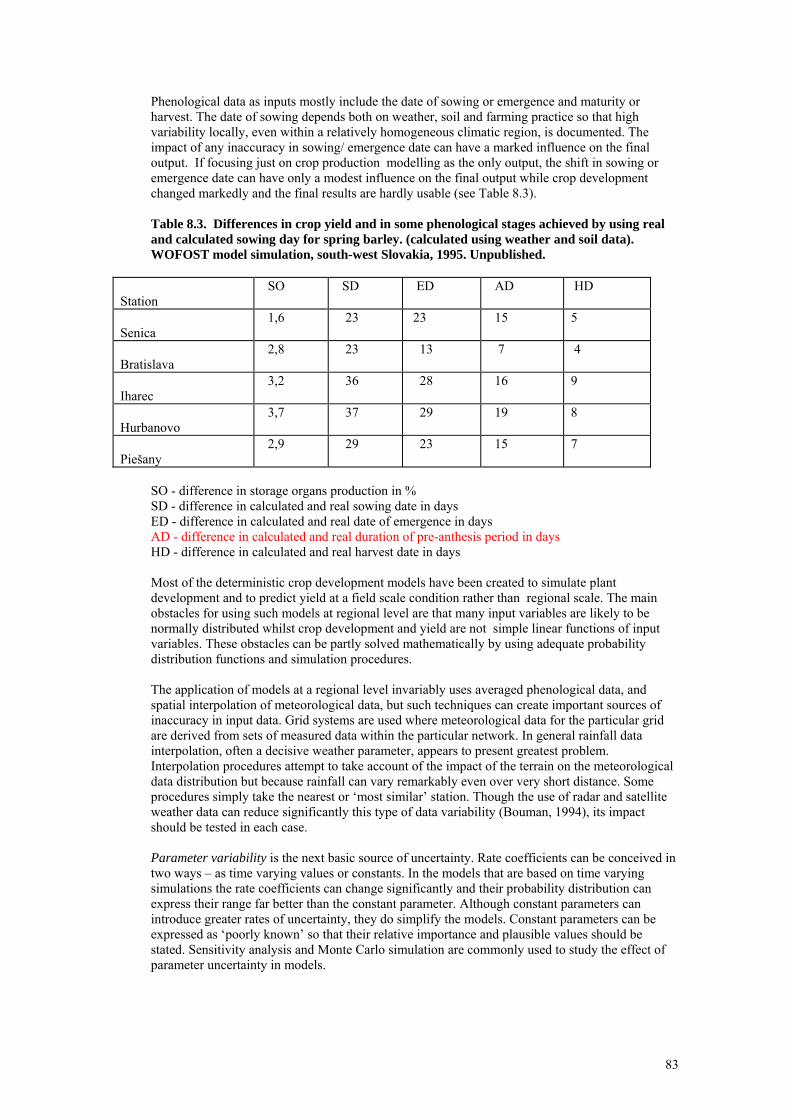
83

Phenological data as inputs mostly include the date of sowing or emergence and maturity or harvest. The date of sowing depends both on weather, soil and farming practice so that high variability locally, even within a relatively homogeneous climatic region, is documented. The impact of any inaccuracy in sowing/ emergence date can have a marked influence on the final output. If focusing just on crop production modelling as the only output, the shift in sowing or emergence date can have only a modest influence on the final output while crop development changed markedly and the final results are hardly usable (see Table 8.3). Table 8.3. Differences in crop yield and in some phenological stages achieved by using real and calculated sowing day for spring barley. (calculated using weather and soil data). WOFOST model simulation, south-west Slovakia, 1995. Unpublished.

Station

SO SD ED AD HD

Senica

1,6 23 23 15 5

Bratislava

2,8 23 13 7 4

Iharec

3,2 36 28 16 9

Hurbanovo

3,7 37 29 19 8

Piešany

2,9 29 23 15 7

SO - difference in storage organs production in % SD - difference in calculated and real sowing date in days ED - difference in calculated and real date of emergence in days AD - difference in calculated and real duration of pre-anthesis period in days HD - difference in calculated and real harvest date in days Most of the deterministic crop development models have been created to simulate plant development and to predict yield at a field scale condition rather than regional scale. The main obstacles for using such models at regional level are that many input variables are likely to be normally distributed whilst crop development and yield are not simple linear functions of input variables. These obstacles can be partly solved mathematically by using adequate probability distribution functions and simulation procedures. The application of models at a regional level invariably uses averaged phenological data, and spatial interpolation of meteorological data, but such techniques can create important sources of inaccuracy in input data. Grid systems are used where meteorological data for the particular grid are derived from sets of measured data within the particular network. In general rainfall data interpolation, often a decisive weather parameter, appears to present greatest problem. Interpolation procedures attempt to take account of the impact of the terrain on the meteorological data distribution but because rainfall can vary remarkably even over very short distance. Some procedures simply take the nearest or ‘most similar’ station. Though the use of radar and satellite weather data can reduce significantly this type of data variability (Bouman, 1994), its impact should be tested in each case. Parameter variability is the next basic source of uncertainty. Rate coefficients can be conceived in two ways – as time varying values or constants. In the models that are based on time varying simulations the rate coefficients can change significantly and their probability distribution can express their range far better than the constant parameter. Although constant parameters can introduce greater rates of uncertainty, they do simplify the models. Constant parameters can be expressed as ‘poorly known’ so that their relative importance and plausible values should be stated. Sensitivity analysis and Monte Carlo simulation are commonly used to study the effect of parameter uncertainty in models.

84

8.3.2 Accuracy of Pest and Disease Models Much of what was written in the previous section about crop development applies to pest and disease models. The following section identifies areas in which the latter models differ from crop growth models. One should also keep in mind that the driving impetus for pest and disease simulation models is somewhat different from that for crop models: thus most pest and disease simulation models take on a flavour of pest management. The different goals that modellers had in mind in turn led to different kinds of pest and disease models. They can be roughly divided into three major groups, although there are some that would dispute whether the first two are simulation models at all. These groups are: Decision Rules are often referred to as models. They can be the result of process models, and often require similar data. These models produce advice regarding pest control measures, and can (in their most complicated form) even contain simple simulations of pests. In their simplest form, however, they are merely rules that give advice as a function of environmental and other variables. Descriptive Models are usually derived statistically from pest or disease data. They try and derive relatively simple statistics regarding population increases (simple exponential growth, for example) over the entire growing season. A typical statistic would be the apparent infection rate, which assumes that the instantaneous rate of disease increase is the product of a constant (the apparent infection rate), the amount of disease and a correction factor equal to the maximum amount of disease minus the amount of actual disease (Vanderplank, 1963). Process Models are the most similar to classic crop growth models,in that the life-cycle of the pest or pathogen is modelled in a manner similar to a plant. In these, the passage through the various stages of a pest's life cycle, or the growth and dispersal of a pathogen are modelled as a function of a number of different environmental factors. These models can take on a range of detail, from models that simulate an entire field as a single unit, to models that simulate disease processes on different leaves and flowers of a single plant. The detail in these models usually requires comprehensive , local weather data. The latter group can be further divided into two groups. Historically, the first disease and pest models were concerned with modelling the growth of insect pests or pathogens, and the fact that these were dependent on (and indeed growing on) plants was of secondary importance. These models didn't simulate the growth of the plant at all, and if the plant was even recognised in the model, it's growth consisted of a lookup table describing the LAI, biomass, or phenology, at different times during the growing season. In contrast, there is a second group of models, often referred to as linked models, where one or many pests or pathogens are coupled to a plant growth model. These coupled models are driven by the same or different external variables. The interaction between the pest(s) and the crop plant can also be modelled dynamically, such that the pests are able to affect the crop model (cf. the table of Boote's) and the information regarding the crop affects the pathogen model. An example of this latter interaction is the dispersal of Stagonospora nodorum conidia as a function of the height of the leaves above the ground (Djurle and Yuen, 1991). Coupled models are often produced in stepwise fashion. A pest or disease model may be developed with little or no simulation of the host plant substrate. At a later stage, this substrate could be simulated as a simple model, but no interaction between the models is considered. Finally, the models become equals with a defined two-way interaction.This, of course, is being written by plant pathologists and agronomists might well reverse the roles of the pest and the plant growth model. Pest and disease models can also be used in a number of different ways. Depending on the detail in a coupled model, the effects of plant pests or diseases, and different management strategies of those pests or diseases, can be investigated by comparing different model runs. By making a large number of runs, with historical or even simulated weather data, decisions regarding the best control strategies can be made.

85

Changes in farming practice can also be tested using these models, assuming that the relevant processes are present in the respective models. Questions that could be answered include changes in planting dates, spacing, and even cropping sequences. The models can be used as research tools. One can examine the interrelationships between crop and pest and disease models, and thus gain a better understanding of the different processes. One can, for example, discover the 'weakest point' in the life cycle of the pest or pathogen. Improved, coupled models will lead to better understanding of the effects of pests on crop growth and yield. While it is unlikely that complex, process-based models will receive direct, widespread use in agricultural production, they can lead to decision rules, which can be used for disease and pest prediction. If these process models are coupled to growth models, yield loss prediction will also be possible. Assistance in making decisions during the growing season (tactical decisions), as well as long-term strategies for agricultural production, will be possible. Data quality is important. For the coupled models the presence and absence (and even severity) of diseases or pests infestations on different parts of the plant (phenologically defined plant units) such as flowers, stems leaves and tubers will be necessary for model construction and validation. The microenvironment within the plant canopy is important for process based models, and a thorough understanding of the relationship between screen variables and conditions within the canopy is of uttermost importance. Statistically derived models (such as decision rules and descriptive models) can theoretically work with any quality of data. However, the latter does affects the quality of the results, and poor quality data will lead to uncertain estimates with larger variance.

8.4. Calibration and validation of the models

8.4.1 Generally about phenological models of crops The complexity of the calibration of phenological models comes from the number of parameters or relationships which have to be tested before the model can be locally adapted. For the ARCWHEAT development model the adaptation to other wheat varieties can be achieved by changing Tb, Pb, the parameters (T1, T2, T3 and T4) and the form of the vernalization effectiveness function Veff and the parameters (Vb and Vsat) of the normalized vernalization factor i(V). The thermal times to reach the main phenological stages may also be modified. Genetic sensitivity should at least partially be determined a priori, and the remaining parameters estimated from experiments. It may be also expected that a group of varieties which are adapted to a specific environment have more or less similar development rhythm. In that case the phenology model could be applied to other varieties without having to proceed to heavy calibration procedures. The optimization procedure may be conducted in different ways either emprically (Reinink et al 1986) by changing one set of parameters independently of the others or by optimization procedures using maximum likelihood estimation (Travis et al, 1988). The later method demands large samples of observed data as compared to the number of parameters under estimation. The phenological phases are not necessarily mutually independent, so that the parameter values for all phases should be estimated simultaneously, a process which adds some complexity to the problem. As the number of parameters becomes large, the multiplicative form of the model also gives estimated values which are highly correlated so that the choice of a particular optimum combination of the parameters can be meaningless and invalidate the possible use of the model for an other set of data. As a criterion for the performance of a model with different parameter values, the prediction of the anthesis is generally used. This stage has the advantage to be determined quite precisely and is least affected by environmental variability. Most variety differences also arise during the emergence to anthesis phase. The optimum values of the parameters are assessed as those that minimize the residual standard deviation of the photo-vernal-thermal time between two phenological stages expressed as a number with denomination and not as a percentage of the mean

86

value. The effectiveness of the calibration may also be measured by the standard error in days calculated on the deviations between model estimates and observed dates of phenological stages. The mean difference between observed and predicted dates has also to be taken into account to assess the performance of the model. It is supposed that an unbiased solution can be obtained by an adequate calibration procedure. In general the precision of the model varies with the phenological stage considered, estimation of the earliest stages being subject to greater uncertainty. Travis et al, (1988) after optimizing the parameters of the ARCWHEAT model in the U.K. give residual standard errors of 8.4 and 7.2 days for the predicted dates of double ridges and terminal spikelet stages. In France Delecolle and Guerif (1986) give values of 6.5 and 5.4 days for beginning of stem elongation and anthesis. Testing the performances of development models over a wide range of varieties and environments in Belgium, Oger (1998) found a standard deviation of 5.4 days for the prediction of the duration of the sowing to heading phase and 5.1 days for heading to maturity for winter wheat.

8.4.2 Validation of crop development models Models reflect reality, but do not represent it identically. It means that the model corresponds to the original in some particular aspects while in other aspects it can differ considerably. Despite this fact the model can describe some phenomena and also identify relationships between them. Before using the model-knowledge about the significance of the correspondence of the model and reality is presupposed. A certain analogy between the model and reality exists on various levels: the level of the outputs, the level of the structures that are in the model represented mostly by a system of functions and the level of elements of these structures. Crop development models are usually complicated systems of equations that involve sets of parameters and inputs. The scope, value and distribution function of the parameter responses has to be known. One possible way of identifying the model parameters is to use the generally justified values in the calibration and to analyse the model outputs according to the experimental data. The deviations of the simulated outputs from the measured data are the criterion of parameter validation: an analysis of this validation may result in new adjustments to parameters. The parameters can be obtained also by using experimental data in the derivation of the model and adjusting the parameters to make the simulation fit the original data (Sands et al., 1979). So the calibration of the model has to proceed its tuning before running the calculation. According to the character of the simulation, inputs and outputs the calibration can proceed on two levels, when the result of calibration is a single optimal vector or a set of parameter vectors that are compatible with the calibration data. Thus the final results of calibration are interpreted as discrete values of the parameters or probability distribution. Following the calibration process one has to respect the fact that the adjusted parameters have to move within the physically possible range. In general there are the crop development models focused just on one specific crop but multicrop models have prevailed recently. Because of this fact specific calibration has to be performed for each set of parameters for the particular crop and locality (region). The transportability of the deterministic models also requires the user to set limitation parameters. Literature reviews and expert knowledge are necessary for initial setting of soil and crop parameters before calibration. Soil parameters are generally difficult to obtain and mostly they are estimated from existing soil maps. Though soil parameters can be conceived as a set of constants according to the soil type, their high spatial variability requires recurrent calibration to set the marginal values. This phenomenon together with the temporal variability of crop parameters and non-calibrated parameters are one of the basic sources of model uncertainty. Regarding this effect an uncertainty analysis should be executed after calibration if the level of uncertainty of the outputs is acceptable for the application. The use of model simulation requires the description of the model from the perspective of representative outputs. This demand is not always fully fulfilled, since for example, MacKerron (1992) quotes just five adequate validations out of 19 potato growth models. To test the model for the accuracy and adequacy two steps are recommended: validation and verification. These expressions can be understood in various ways. As for verification we shall consider the process when the model is submitted to the evaluation of its logical construction, program compilation and searching for syntax errors. The model (program) can be run for the cases when the outputs are already known and formal errors in program coding are detected.

87

Validation should be conceived as an investigation of correctness and appropriateness of the model. To validate the model does not mean only the simple comparison of model outputs to measured (experimental or statistical) data. Generally the agreement between simulated and real data is only one step of validation. Meaningful validation establishes whether or not the model produces results that are generally consistent with the data to which they are compared and can be explained in terms of the parameters (crop variety, soil type, farming practices, weather conditions etc.) applied through the model. Firstly it is necessary to define the basic aim of the model that should be validated. Consequently the model structure and its components are investigated qualitatively; if they do reflect adequately the hypothesis of the model and the adequacy and accuracy of the parameters, then variables and outputs should be analysed quantitatively. Validation of the model is more complicated than verification. At this step two extreme situations can occur. Firstly in the case when a good formulated model produces incorrect outputs because of an indequate level of simplification of its components or some important variable or parameters are omitted, e.g. simple crop production model based just on incident radiation. The degree of precision of the model defines its resolution power. If it is too low the model is not able to express some influences of the reality and so more elements (variables) need to be considered. On the other hand the complicated model with abundant parameters leads to an increased number of errors and a higher level of uncertainty. In a specific situation even the model that includes some error can produce plausible outputs, the magnitude of which is within the scale of measured data. Such a situation can occur when the mathematical formulas are valid for a restricted range of input data. In this case the outputs are in accord with experimentally measured data while beyond this range the simulation produces false results. This indicates the necessity to cover the whole scale of possible inputs and parameters on which the model could be tested and to analyse step by step which component of the model could be wrong. To validate models the following general procedures are recommended: 1. To run the model for the extreme values of the inputs 2. To run the model on independent set(s) of inputs and to compare the outputs to empirical data and to inspect the adequacy of the hypothesis used for the model formulation 3. Sensitivity analysis 4. To evaluate the acceptable errors and accuracy according to the purpose of the model The basic criterion of validation is to compare the results of simulation to completely independent data sets. Even by using such data the validation is weighted with an uncertainty that is a consequence of the uncertainty of the experimental (statistical) data to which the results of simulation are compared. When the information about the measurement error of the independent data set is not available the validation becomes less confident or is impossible (Jansen, 1994). The confidence of the validation can be improved by using different sources of independent statistical datasets or by duplicate measurements. This is usually possible when testing the model at the regional scale where various sources of statistical data could be available. In such cases the perfect agreement of simulated and statistical data can hardly occur but this feature is also dependent on the initial conditions of the validated components of the model outputs. When to using the model on a regional scale the most frequent obstacle in validation is the fact that the model requires point input data and gives point output data that are not generally representative of the region. Under such condition the model simulation can sharply deviate from the real data because of extreme local weather conditions or other parameters while for the most part of the simulation they agree well. Inaccuracy at the input data can produce various changes in the outputs. The sensitivity of the model can be investigated by various types of sensitivity analysis and multiple running of the model when inputs are varied. The task is to inspect the impact of variation in inputs data and design on the character of the outputs and also to define the magnitude of the change of the particular output. A commonly used method to state the behaviour of the output according to the input change is so called "one at a time" sensitivity analysis where a response to variation of one input is studied whereas the other inputs are kept at nominally defined values. Output analysis can finally show the weight of the particular input, its change, etc.. This change can vary remarkably and the dependency on the input change is always not linear. The results of such analysis can be

88

expressed as discrete values (Table 8.4) or in the case of the gradual frequent change of the particular input in the form of a graph where the discontinuities can be detected. Table 8.4. Change in accumulated dry matter considering ±5 and ±10% modifications of the original values

Parameter -10 % -5 % +5 % +10 % Available water capacity -2.07 % -0.63 % 0.67 % 1.35 % Maximal root depth -4.89 % -2.77 % 3.48 % 6.82 % Daily mean temperature 41.90 % 23.37 % -22.82 % -42.89 % Precipitation -9.78 % -4.57 % 3.95 % 6.97%

Source - Bussay A. and Szinell Cs. : A Simple Model for Estimating the Impact of Climate Change on the Potato Productions in Hungary , Manuscript Quantifying the magnitude of the sensitivity of the particular input allows one to claim a degree of accuracy of this input. But the magnitude of the output change is not always the only criterion of the model sensitivity to the particular input. Such a criterion can be also expressed as a change in time, e.g. the maximum of the crop growth curve or its position on the time scale.

8.4.3 Validation of Pest and Disease Models The validation of process based models of pests and diseases can be carried out in a manner similar to those for crop growth. This involves the validation and verification processes mentioned for the growth models and a sensitivity analysis where the effects of changes in parameters on model results are checked. Obviously, data is also needed for the validation and verification procedures, as for the crop growth models, with the added requirement for suitable pest or disease incidence and/ or severity levels recorded at several points during the growing season. A different method can be used in the validation of descriptive relationships, where statistical methods are used to estimate parameters in relationships between weather or other climatic variables and pest or pathogen growth or reproduction. These relationships are statistical in nature, and their validation can take a statistical form. Thus, in addition to the actual parameters, variances (standard deviations or confidence intervals) for the parameters can also be presented. Since the relationships themselves are conditional on the data used to develop them, it can be useful to calculate predicted values for an independent data set and examine the predicted and observed values. Thus, if the relationship between development rates and weather are estimated from one data set, this can be tested with another data set. Validation of decision rules is similar to that of the statistically defined relationships. Thus an independent data set (that was not used in the development of the decision rules) can be used to test the performance of the decision rules. The concepts of sensitivity and specificity of the predictors should be introduced as measures of the performance of the predictor (Yuen et al, 1996). Briefly stated, the proportion of correct predictions with regards to implementing the control measure is referred to as sensitivity. The correct decision not to implement the control measure is referred to as specificity. Both of these measure of the performance of a predictor. These can be seen in Table 1, where A/A+C refers to the sensitivity, and D/B+D refers to the specificity of a predictor. Event Occurs

Yes No Event Predicted Yes A B

No C D Table 8.5 Four possible outcomes in event prediction The frequency of incorrect decisions (C/A+C and B/B+D in the Table 8.5) and the costs of making these mistakes also have to be considered in the evaluation of prediction algorithms.

89

References and additional reading Addiscot,T.M., (1993), Simulation modelling and soil behaviour, Geoderma, 60, 15 -40

Bouman,B.A.M., (1994), Yield prediction by crop modelling and remote sensing. In: Dallemand, J. F., Vossen, P. (1996), Agrometeorological Models: Theory and Applications in the MARS Project, Luxembourg, Office for Officical Publications of the European Communities, ECSC – EC – EAEC Brussels Luxembourg Bussay, A. and Szinell, C., (1994), A Simple Model for Estimating the Impact of Climate Change on the Potato productions in Hungary, Manuscript (Unpublished) Delecolle, R. and Guerif, M. (1986), Les modèles agrométéorologiques de développment, INRA Note interne No M86/9, 61 p Djurle, A.M. and Yuen, J. (1991), A simulation model for septoria nodorum in winter wheat, Agricultural Systems 37: 193-218 Doraiswamy P. C., and Thomson, D.R. (1982), A crop moisture stress index for large areas and its application in the prediction of spring wheat phenology, Agricultural and Forest Meteorology 27, 1-15 Fagerberg,B., 1995 : Crop growth models, pest damage and regional yield forecasts, In. SP - Report ,In: Danish Institute of Plant and Soil Science, 10 Godske, C. L., (1966), Statistikk i forskning og praksis, Universitetsforlaget, in Norwegian Goudriaan, J., (1977), Crop micrometeorology: a simulation study, Simulation monographs, Pudoc, Wageningen, 249 pp. Hough, M.N., Chalmers, I. F., and Flockhardt, I, (1990), Scheduling winter barley crop management using a growth stage model, Proceeedings of a symposium, The Agrometeorology of Rainfed Barley-Based Farming Systems, Tunis 6 – 10 March 1989, WMO. Jansen, M. J. W. (1994), Validation of CGMS, . In: Dallemand, J. F., Vossen, P. (1996), Agrometeorological Models: Theory and Applications in the MARS Project, Luxembourg: Office for Officical Publications of the European Communities, ECSC – EC – EAEC Brussels Luxembourg Jansson, P.E. (1990), Soil water and heat model, Technical description, Department of soil sciences, Uppsala , Sweden Kaukoranta, T., Hannukkala, and Tahvonen, R. (1993), Weather-based disease warning device Proc. Workshop on Computer-based DSS, Parma, Italy 23-26 Nov 1993, SP Report (Danish Inst. Of Plant and Soil Sci. ) No 7. 147 –154 MacKerron, (1992), Agrometeorlogical aspects of forecasting yields of potato within the E. C., Luxembourg: Office for Officical Publications of the European Communities, ECSC – EC – EAEC Brussels Luxembourg Norman, J. (1982), Simulation of microclimates, in Biometeorolgy in integrated pest managemenbt, eds. Hatfield, J. L., and Thomason, J.J., Academic Press Oger, R.,(1998), Performance and comparison of wheat simulation models in presence of genotype x environment interaction, Proceedings from International Symposium on Applied Agrometeorology and Agroclimatology, Volos 1996, European Commission. Reinink K., Jorrisma J., and Darwinkel, A. (1986), Adaption of AFRC wheat phenology model for Dutch conditions, Netherlands Journal of Agricultural Science 34, 1 - 13

90

Penning de Vries, F. W. T. and Spitters, C. J. T. (1991), The potential for improvement in crop yield simulation. In: Muchow, R. C. And Bellamy, J. A., (eds.) (1991), Climatic risk in crop production: models and management for semiarid tropics and subtropics. CAB- International, Wallingford, 123 – 140. Sands, P. J., hackett, C. , and Nix, H.A. (1979), A model of the development and bulking of potatoes (Solanum tuberosum L.) In: deviation from well managed field crops. Field crops research, 2: 309-331. Söderström, M., and Magnusson, B. (1995), Assessment of local agroclimatological conditions - a methodology, Agricultural and Forest Meteorology, 72, 243 -260 Travis K.Z., Day M, and Porter J.R.(1988), Modelling the timing of the early development of winter wheat, Agricultural and Forest Meteorology 44, 67 -79 Vidoviè,J., (1994), Logical principles and experimental verificatiom of MACROS model, In:Modely a modelovanie rastlinnej produkcie, VŠP Nitra (in Slovak) Vanderplank, J. E. (1963), Plant Diseases: Epidemics and Control, Academic Press Waggoneer, P.E., Furnival, G. M., and Reifsnyder, E.,(1969), Forest Sci., 15, 37 -45 Wieringa, J., ( September 1996), Enquiry review by EC-COST Action 711 , Publ. EC-DG-XII, Brussel WMO (1994), Practical use of agrometeorological data and information for planning and operational activities in agriculture , WMO, TD-No.629, CagM report No. 60, Geneva Øgland, P., 1995: Automatisk datakontroll for SYNOP og AUTO: ADK v.2.0, Rapport nr.12/95 KLIBAS, Det norske meteorologiske institutt.,In Norwegian Øgland, P., 1996: Kvalitetskontroll av automatstasjonsdata januar 1996, Rapport nr.04/96 KLIBAS, Det norske meteorologiske institutt, In Norwegian

91

9.What kind of work is needed in the future? In the introduction to this report the objectives of the report writing are summarised to clarify: (a) The existence of useful models. (b) How it may be possible to use the existing models operationally in plant protection? (c) How should future research and development be organised to improve existing operational models and construct new operational models in this context? In this concluding chapter it remains to say something about future research and development. Research and development is organised in a variety of ways in the different countries of Europe, but in them regional or central organisations will collect and disseminate meteorological and biological data, and some organisations will also disseminate plant protection warnings to farmers. It therefore seems possible to say something about research and development, relevant for most of Western and Southern Europe and parts of Eastern Europe. A model used in plant protection consists as a rule of some of the following subsystems: Atmosphere – soil –crop – pathogen/ pest. Most models need both meteorological and biological input data. Improvements in the warning systems can be achieved by collecting better meteorological data, by obtaining better biological data, by uncovering new biological/ meteorological relationships and implementing these relationships, and by improving the dissemination part of the warning system. We have in this report discussed the concept of quality of meteorological data, and we have discussed different techniques of obtaining meteorological data, both by measurement and by using prognostic data. In the future it will probably be possible to obtain meteorological data at the canopy level, in addition to traditional measurements in a Stevenson screen, by using some sort of extrapolation or interpolation of the data measured. It will also probably be possible to use GIS-techniques in the future to extend measurements at several known points to the region considered. The biological subsystem considered consists of the crop and the pathogen or pest. Enormous amounts of knowledge of these biological subsystems are available for the major pest/ pathogen, but only some of the relevant knowledge has been implemented into operational numerical, quantitative models. One is tempted to presume that better meteorological data, at the canopy level and at a regional level could be used in the future to give us several new and interesting relationships connecting biology and the meteorology. The main problem now seems to be our lack of ability to implement existing biological knowledge in models that can be run operationally. Despite its long history, the science of modelling crop, pest and disease phenology is not at an advanced stage of development. Some of the lack of progress may be attributed to the use of an empirical approach. What is needed is a set of deterministic models of the processes in which temperature, photoperiod and humidity affect the phenological processes. Developing crop, pest/ disease phenological models presents an interesting challenge in Europe. There is large variability not only within the growing season but between growing seasons as well. Thus, it is important that phenological models accurately describe development rate at both low and high temperatures, as well as in photoperiodically extreme environments. There is a need to develop phenological models at a minimum of two levels. The first level would be a model to provide a reasonable estimate of phenological development of most of the cultivars of a given species grown in a region. This kind of model would allow us to assess the progress of pests and diseases in winter wheat or barley in Europe related to their phenological development and the duration of the growing season. Such a model would be useful in assessing the risk of a particular cultivar of wheat or barley being affected by apest or a disease in a specified area. Looking at the existing quantitative models combining meteorological and biological data, it is not as a rule easy to test and use these models with new crop varieties and pest/ pathogen races in new

92

locations. The tasks related to model validation are difficult, and it demands much work to acquire the correct biological and meteorological quantitative parameters that are necessary for operational use. One could wish that national research programs could make it possible to thoroughly test and validate models which are operationally used in other regions of Europe. In order to operationally run models and disseminate results the following factors must be fulfilled: (a) Meteorological data of a certain quality must be available. (b) Necessary biological data must be available. (c) The models must be validated and implemented, and the necessary competence to understand

the results that are produced must be available. (d) There must exist some system for the dissemination of the information produced. Regarding the dissemination of plant protection warnings, data and other relevant information it seems to be possible also to use the new technology of the Internet. In the advanced countries of Europe one could think that Internet in the not too distant future could be the most effective medium for dissemination of the information mentioned. In the first place information could be distributed by this medium to the existing public or private extension service. The link between the extension service and the end users, the farmers, will as a rule be the traditional media as telephone, telefax, and the postal system. But in some European countries one also will have an increasing group of farmers connected with their own PC’s to the Internet. It could also be relevant to mention ‘precision farming’. In this area of research GPS (global positioning system)- methods are used to increase the details of the information on agronomy, crop, soil chemistry, soil physics etc. of each of the farmers fields. In order to use results from research in ‘precision farming’ operationally on a larger scale it is probably necessary to define parameters and develop new methods for economically and effectively measuring and calculating parameters of the soil, crop etc. on a much smaller scale and much more accurately than what is possible now. Similar problems are connected to the efforts of getting and using meteorological data at the canopy level in plant protection. One would also like to point at the hypothetico-deductive method, outlined in chapter 8, in connection with the implementation of models and operational use of models. I t seems possible in a world connected by the Internet, very systematically to put thorough documentation of the models used by every organisation into databases available for every one. Every single step in the definition and validation process of each model ought to be documented, how measurements are actually done, how parameters are actually found, how the subsystems are tested, how the complete system is tested, and which instruments are used in both the validation process and in operational use.