The Periodic Unfolding Method in Homogenization

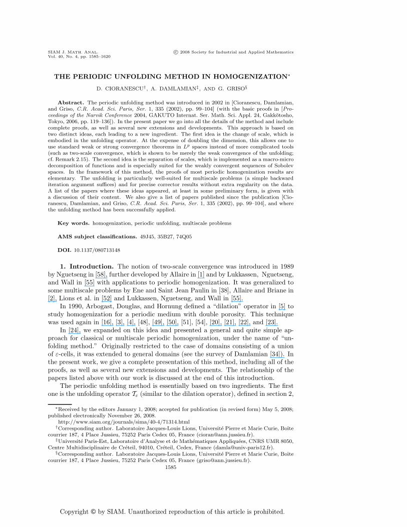
Copyright © by SIAM. Unauthorized reproduction of this article is prohibited.

SIAM J. MATH. ANAL. c© 2008 Society for Industrial and Applied MathematicsVol. 40, No. 4, pp. 1585–1620

THE PERIODIC UNFOLDING METHOD IN HOMOGENIZATION∗

D. CIORANESCU† , A. DAMLAMIAN‡, AND G. GRISO§

Abstract. The periodic unfolding method was introduced in 2002 in [Cioranescu, Damlamian,and Griso, C.R. Acad. Sci. Paris, Ser. 1, 335 (2002), pp. 99–104] (with the basic proofs in [Pro-ceedings of the Narvik Conference 2004, GAKUTO Internat. Ser. Math. Sci. Appl. 24, Gakkotosho,Tokyo, 2006, pp. 119–136]). In the present paper we go into all the details of the method and includecomplete proofs, as well as several new extensions and developments. This approach is based ontwo distinct ideas, each leading to a new ingredient. The first idea is the change of scale, which isembodied in the unfolding operator. At the expense of doubling the dimension, this allows one touse standard weak or strong convergence theorems in Lp spaces instead of more complicated tools(such as two-scale convergence, which is shown to be merely the weak convergence of the unfolding;cf. Remark 2.15). The second idea is the separation of scales, which is implemented as a macro-microdecomposition of functions and is especially suited for the weakly convergent sequences of Sobolevspaces. In the framework of this method, the proofs of most periodic homogenization results areelementary. The unfolding is particularly well-suited for multiscale problems (a simple backwarditeration argument suffices) and for precise corrector results without extra regularity on the data.A list of the papers where these ideas appeared, at least in some preliminary form, is given witha discussion of their content. We also give a list of papers published since the publication [Cio-ranescu, Damlamian, and Griso, C.R. Acad. Sci. Paris, Ser. 1, 335 (2002), pp. 99–104], and wherethe unfolding method has been successfully applied.

Key words. homogenization, periodic unfolding, multiscale problems

AMS subject classifications. 49J45, 35B27, 74Q05

DOI. 10.1137/080713148

1. Introduction. The notion of two-scale convergence was introduced in 1989by Nguetseng in [58], further developed by Allaire in [1] and by Lukkassen, Nguetseng,and Wall in [55] with applications to periodic homogenization. It was generalized tosome multiscale problems by Ene and Saint Jean Paulin in [38], Allaire and Briane in[2], Lions et al. in [52] and Lukkassen, Nguetseng, and Wall in [55].

In 1990, Arbogast, Douglas, and Hornung defined a “dilation” operator in [5] tostudy homogenization for a periodic medium with double porosity. This techniquewas used again in [16], [3], [4], [48], [49], [50], [51], [54], [20], [21], [22], and [23].

In [24], we expanded on this idea and presented a general and quite simple ap-proach for classical or multiscale periodic homogenization, under the name of “un-folding method.” Originally restricted to the case of domains consisting of a unionof ε-cells, it was extended to general domains (see the survey of Damlamian [34]). Inthe present work, we give a complete presentation of this method, including all of theproofs, as well as several new extensions and developments. The relationship of thepapers listed above with our work is discussed at the end of this introduction.

The periodic unfolding method is essentially based on two ingredients. The firstone is the unfolding operator Tε (similar to the dilation operator), defined in section 2,

∗Received by the editors January 1, 2008; accepted for publication (in revised form) May 5, 2008;published electronically November 26, 2008.

http://www.siam.org/journals/sima/40-4/71314.html†Corresponding author. Laboratoire Jacques-Louis Lions, Universite Pierre et Marie Curie, Boıte

courrier 187, 4 Place Jussieu, 75252 Paris Cedex 05, France ([email protected]).‡Universite Paris-Est, Laboratoire d’Analyse et de Mathematiques Appliquees, CNRS UMR 8050,

Centre Multidisciplinaire de Creteil, 94010, Creteil, Cedex, France ([email protected]).§Corresponding author. Laboratoire Jacques-Louis Lions, Universite Pierre et Marie Curie, Boıte

courrier 187, 4 Place Jussieu, 75252 Paris Cedex 05, France ([email protected]).

1585

Copyright © by SIAM. Unauthorized reproduction of this article is prohibited.

1586 D. CIORANESCU, A. DAMLAMIAN, AND G. GRISO

where its properties are investigated. Let Ω be a bounded open set, and Y a referencecell in R

n. By definition, the operator Tε associates to any function v in Lp(Ω), afunction Tε(v) in Lp(Ω × Y ). An immediate (and interesting) property of Tε is thatit enables one to transform any integral over Ω in an integral over Ω× Y . Indeed, byProposition 2.6 below

(1.1)∫

Ω

w(x) dx ∼ 1|Y |

∫Ω×Y

Tε(w)(x, y) dx dy ∀w ∈ L1(Ω).

Proposition 2.14 shows that the two-scale convergence in the Lp(Ω)-sense of asequence of functions {vε} is equivalent to the weak convergence of the sequence ofunfolded functions {Tε(vε)} in Lp(Ω × Y ). Thus, the two-scale convergence in Ωis reduced to a mere weak convergence in Lp(Ω × Y ), which conceptually simplifiesproofs.

In section 2 are also introduced a local average operator Mε and an averagingoperator Uε, the latter being, in some sense, the inverse of the unfolding operator Tε.

The second ingredient of the periodic unfolding method consists of separatingthe characteristic scales by decomposing every function ϕ belonging to W 1,p(Ω) intwo parts. In section 3 it is achieved by using the local average. In section 4, theoriginal proof of this scale-splitting, inspired by the finite element method (FEM), isgiven. The confrontation of the two methods of sections 3 and 4 is interesting in itself(Theorem 3.5 and Proposition 4.8). In both approaches, ϕ is written as ϕ = ϕε

1 +εϕε2,

where ϕε1 is a macroscopic part designed not to capture the oscillations of order ε (if

there are any), while the microscopic part ϕε2 is designed to do so. The main result

states that, from any bounded sequence {wε} in W 1,p(Ω), weakly convergent to somew, one can always extract a subsequence (still denoted {wε}) such that wε = wε

1+εwε2,

with

(1.2)

(i) wε1 ⇀ w weakly in W 1,p(Ω),

(ii) Tε(wε) ⇀ w weakly in Lp(Ω;W 1,p(Y )),

(iii) Tε(wε2) ⇀ w weakly in Lp(Ω;W 1,p(Y )),

(iv) Tε(∇wε) ⇀ ∇w + ∇yw weakly in Lp(Ω × Y ),

where w belongs to Lp(Ω;W 1,pper(Y )).

In section 5 we apply the periodic unfolding method to a classical periodic homog-enization problem. We point out that, in the framework of this method, the proof ofthe homogenization result is elementary. It relies essentially on formula (1.1), on theproperties of Tε, and on convergences (1.2). It applies directly for both homogeneousDirichlet or Neumann boundary conditions without hypothesis on the regularity of∂Ω. For nonhomogenous boundary conditions (or for Robin-type condition), someregularity of ∂Ω is required for the problem to make sense, in which case the methodapplies also directly (see Remark 5.12).

Section 6 is devoted to a corrector result, which holds without any additionalregularity on the data (contrary to all previous proofs; see [11], [30], and [59]). Thisresult follows from the use of the averaging operator Uε. The idea of using averagesto improve corrector results first appeared in Dal Maso and Defranceschi [33]. Wealso give some error estimates and a new corrector result for the case of domains with

Copyright © by SIAM. Unauthorized reproduction of this article is prohibited.

THE PERIODIC UNFOLDING METHOD IN HOMOGENIZATION 1587

a smooth boundary (obtained by Griso in [42], [43], [44], and [45]). These results areexplicitely connected to the unfolding method and improve on known classical ones(see [11] and [59]).

The periodic unfolding method is particularly well-suited for the case of multiscaleproblems. This is shown in section 7 by a simple backward iteration argument. Thisproblem has a long history; one of the first papers on the subject is due to Bruggeman[19]. Its mathematical treatment by homogenization goes back to the book of Bensous-san, Lions, and Papanicolaou [11], where for this problem, the method of asymptoticexpansions is used. For more recent references of multiscale homogenization and itsapplications, we refer to the books of Braides and Defranceschi [17], Milton [57], andthe articles by Damlamian and Donato [35], Lukkassen and Milton [54], Lukkassen[53], Braides and Lukkassen [18], Babadjian and Baıa [6], and Barchiesi [8].

The final section gives a list of papers where the method has been successfullyapplied since the publication of [24].

To conclude, let us turn back to the papers quoted at the beginning of thisintroduction and point out their relationships with our results. The dilation operationfrom Arbogast, Douglas, and Hornung [5] was defined in a domain which is an exactunion of εY -cells. It consists in a change of variables, similar to that used in Definition2.1 below. By this operation, any integral on Ω can be written as an integral overΩ×Y . Some elementary properties of the dilation operator in the space L2 were alsocontained in Lemma 2 of [5].

The same dilation operator was used by Bourgeat, Luckhaus, and Mikelic in [16]under the name of “periodic modulation.” Proposition 4.6 of [16] showed that if asequence two-scale converges and its periodic modulation converges weakly, they havethe same limit.

In the context of two-scale convergence, Allaire and Conca [3] defined a pairof extension and projection operators (suited to Bloch decompositions) which areadjoint of each other. They are similar to our operators Tε and Uε and the equiv-alent of property (2.12) and Proposition 2.18(ii) below, are proved in Lemma 4.2of [3]. These properties were exploited by Allaire, Conca, and Vanninathan in [4]for a general bounded domain by extending all functions by zero on its comple-ment.

In [48], Lenczner used the dilation operator (here called “two-scale transforma-tion”) in order to treat the homogenization of discrete electrical networks (by nature,the domain is a union of ε-cells). The convergence of the two-scale transform iscalled two-scale convergence (this would be confusing except that it was shown to beequivalent to the original two-scale convergence). As an aside, a convergence similarto (1.2)(iv) was also treated. In Lenczner and Mercier [49], Lenczner and Senouci-Bereksi [50], and Lenczner, Kader, and Perrier [51], this theory was applied to periodicelectrical networks.

Finally, Casado Dıaz and Luna-Laynez [21], Casado Dıaz, Luna-Laynez, and Mar-tin [22] and [23] used the dilation operator in the case of reticulated structures. Inthis framework, they obtained the equivalent of (3.7)(i) of Theorem 3.5 below.

2. Unfolding in Lp-spaces.

2.1. The unfolding operator Tε. In Rn, let Ω be an open set and Y a reference

cell (e.g., ]0, 1[n, or more generally, a set having the paving property, with respect toa basis (b1, . . . , bn) defining the periods).

By analogy with the notation in the one-dimensional case, for z ∈ Rn, [z]Y denotes

the unique integer combination∑n

j=1 kjbj of the periods such that z − [z]Y belongs

Copyright © by SIAM. Unauthorized reproduction of this article is prohibited.

1588 D. CIORANESCU, A. DAMLAMIAN, AND G. GRISO

Fig. 1. Definition of [z]Y and {z}Y .

to Y , and set

{z}Y = z − [z]Y ∈ Y a.e. for z ∈ Rn.

Then for each x ∈ Rn, one has

x = ε([xε

]Y

+{xε

}Y

)a.e. for x ∈ R

n (See Figure 1).

We use the following notations:

(2.1)

⎧⎪⎪⎪⎪⎪⎨⎪⎪⎪⎪⎪⎩

Ξε ={ξ ∈ Z

N , ε(ξ + Y ) ⊂ Ω},

Ωε = interior

{ ⋃ξ∈Ξε

ε(ξ + Y

)},

Λε = Ω \ Ωε.

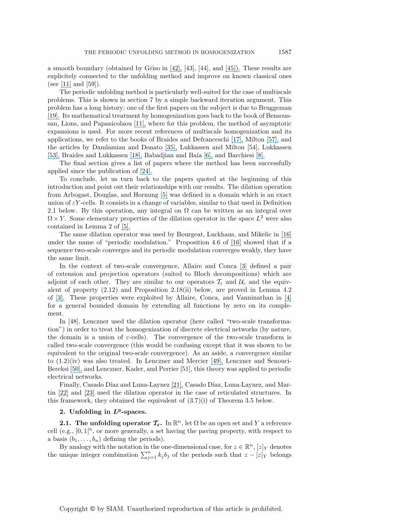
The set Ωε is the largest union of ε(ξ + Y ) cells (ξ ∈ Zn) included in Ω, while Λε is

the subset of Ω containing the parts from ε(ξ+Y

)cells intersecting the boundary ∂Ω

(see Figure 2).Definition 2.1. For φ Lebesgue-measurable on Ω, the unfolding operator Tε is

defined as follows:

Tε(φ)(x, y) =

⎧⎨⎩φ(ε[xε

]Y

+ εy)

a.e. for (x, y) ∈ Ωε × Y,

0 a.e. for (x, y) ∈ Λε × Y.

Observe that the function Tε(φ) is Lebesgue-measurable on Ω × Y and vanishesfor x outside of the set Ωε.

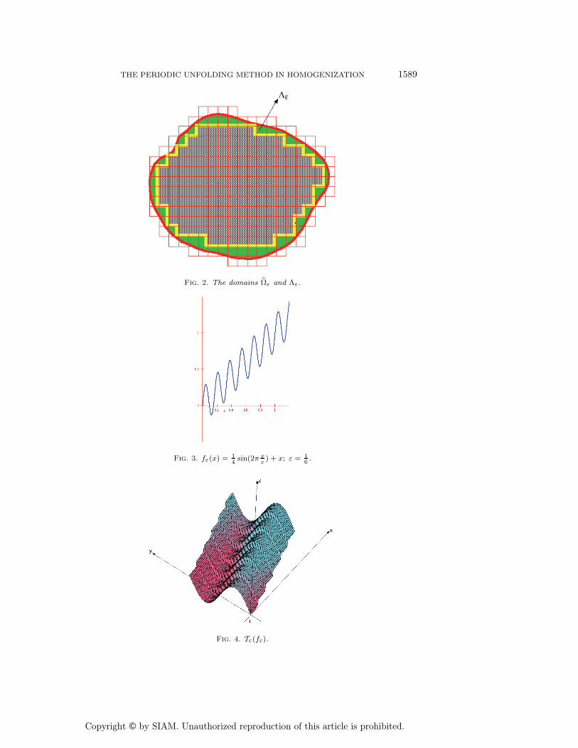
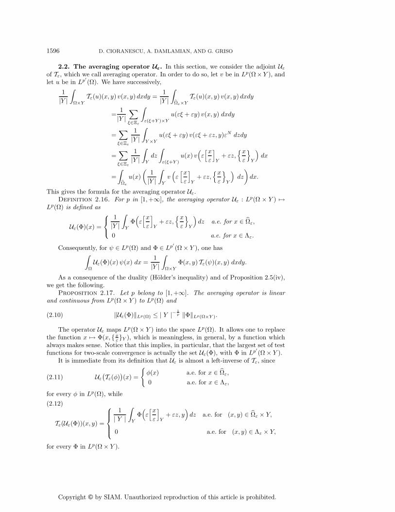
As in classical periodic homogenization, two different scales appear in the defi-nition of Tε: the “macroscopic” scale x gives the position of a point in the domainΩ, while the “microscopic” scale y (= x/ε) gives the position of a point in the cellY . The unfolding operator doubles the dimension of the space and puts all of theoscillations in the second variable, in this way separating the two scales (see Figures 3,4 and Figures 5, 6).

The following property of Tε is a simple consequence of Definition 2.1 for v andw Lebesgue-measurable; it will be used extensively:

(2.2) Tε(vw) = Tε(v) Tε(w).

Copyright © by SIAM. Unauthorized reproduction of this article is prohibited.

THE PERIODIC UNFOLDING METHOD IN HOMOGENIZATION 1589

Fig. 2. The domains Ωε and Λε.

Fig. 3. fε(x) = 14

sin(2π xε) + x; ε = 1

6.

Fig. 4. Tε(fε).

Copyright © by SIAM. Unauthorized reproduction of this article is prohibited.

1590 D. CIORANESCU, A. DAMLAMIAN, AND G. GRISO

Fig. 5. fε = f({xε}Y ).

Fig. 6. Tε(fε).

Another simple consequence of Definition 2.1 is the following result concerning highlyoscillating functions.

Proposition 2.2. For f measurable on Y , extended by Y -periodicity to the wholeof R

n, define the sequence {fε} by

(2.3) fε(x) = f(xε

)a.e. for x ∈ R

n.

Then

Tε(fε|Ω)(x, y) =

{f(y) a.e. for (x, y) ∈ Ωε × Y,

0 a.e. for (x, y) ∈ Λε × Y.

If f belongs to Lp(Y ), p ∈ [1,+∞[, and if Ω is bounded,

(2.4) Tε(fε|Ω) → f strongly in Lp(Ω × Y ).

Remark 2.3. An equivalent way to define fε in (2.3) is to take simply fε(x) =f({x

ε }Y ). For example, with

f(y) =

{1 for y ∈

(0, 1/2

),

2 for y ∈(

1/2, 1),

fε is the highly oscillating periodic function, with period ε from Figure 5.

Copyright © by SIAM. Unauthorized reproduction of this article is prohibited.

THE PERIODIC UNFOLDING METHOD IN HOMOGENIZATION 1591

Remark 2.4. Let f in Lp(Y ), p ∈ [1,+∞[, and fε be defined by (2.3). It iswell-known that {fε|Ω} converges weakly in Lp(Ω) to the mean value of f on Y , andnot strongly unless f is a constant (see Remark 2.11 below).

The next two results, essential in the study of the properties of the unfoldingoperator, are also straightforward from Definition 2.1.

Proposition 2.5. For p ∈ [1,+∞[, the operator Tε is linear and continuousfrom Lp(Ω) to Lp(Ω × Y ). For every φ in L1(Ω) and w in Lp(Ω),

(i)1|Y |

∫Ω×Y

Tε(φ)(x, y) dx dy =∫

Ω

φ(x) dx−∫

Λε

φ(x) dx =∫

Ωε

φ(x) dx,

(ii)1|Y |

∫Ω×Y

|Tε(φ)| dxdy ≤∫

Ω

|φ| dx,

(iii)∣∣∣∣∫

Ω

φdx − 1|Y |

∫Ω×Y

Tε(φ) dxdy∣∣∣∣ ≤ ∫

Λε

|φ| dx,

(iv) ‖Tε(w)‖Lp(Ω×Y ) = | Y |1p ‖w 1Ωε

‖Lp(Ω) ≤ | Y |1p ‖w‖Lp(Ω).

Proof. Recalling Definition 2.2 of Ωε, one has

1|Y |

∫Ω×Y

Tε(φ)(x, y) dx dy =1|Y |

∫Ωε×Y

Tε(φ)(x, y) dx dy

=1|Y |

∑ξ∈Ξε

∫(εξ+εY )×Y

Tε(φ)(x, y) dx dy.

On each (εξ+εY )×Y , by definition, Tε(φ)(x, y) = φ(εξ+εy) is constant in x. Hence,each integral in the sum on the right-hand side successively equals∫

(εξ+εY )×Y

Tε(φ)(x, y) dx dy = |εξ + εY |∫

Y

φ(εξ + εy) dy

= εn|Y |∫

Y

φ(εξ + εy) dy = |Y |∫

(εξ+εY )

φ(x) dx.

By summing over Ξε, the right-hand side becomes∫Ωεφ(x) dx, which gives the

result.Property (iii) in Proposition 2.5 shows that any integral of a function on Ω is

“almost equivalent” to the integral of its unfolded on Ω× Y ; the “integration defect”arises only from the cells intersecting the boundary ∂Ω and is controlled by its integralover Λε.

The next proposition, which we call unfolding criterion for integrals (u.c.i.),is a very useful tool when treating homogenization problems.

Proposition 2.6 (u.c.i.). If {φε} is a sequence in L1(Ω) satisfying∫Λε

|φε| dx→ 0,

then ∫Ω

φε dx− 1|Y |

∫Ω×Y

Tε(φε) dxdy → 0.

Based on this result, we introduce the following notation.

Copyright © by SIAM. Unauthorized reproduction of this article is prohibited.

1592 D. CIORANESCU, A. DAMLAMIAN, AND G. GRISO

Notation. If {wε} is a sequence satisfying u.c.i., we write∫Ω

wεdxTε� 1

|Y |

∫Ω×Y

Tε(wε) dxdy.

Proposition 2.7. Let {uε} be a bounded sequence in Lp(Ω), with p ∈]1,+∞]and v ∈ Lp′

(Ω) (1/p+ 1/p′ = 1), then

(2.5)∫

Ω

uεv dxTε� 1

|Y |

∫Ω×Y

Tε(uε)Tε(v) dxdy.

Suppose ∂Ω is bounded. Let {uε} be a bounded sequence in Lp(Ω) and {vε} a boundedsequence in Lq(Ω), with 1/p+ 1/q < 1, then

(2.6)∫

Ω

uεvεdxTε� 1

|Y |

∫Ω×Y

Tε(uε)Tε(vε) dxdy.

Proof. Observe that 1Λε(x) → 0 for all x ∈ Ω. Consequently, by the Lebesguedominated convergence theorem, one gets

∫Λε

|v|p′dx→ 0, and then by the Holder in-

equality,∫Λε

|uεv| dx→ 0. This proves (2.5). If ∂Ω is bounded, then one immediatelyhas |Λε| → 0 when ε→ 0, and this implies (2.6).

We now investigate the convergence properties related to the unfolding operatorwhen ε → 0. For φ uniformly continuous on Ω, with modulus of continuity mφ, it iseasy to see that

supx∈Ωε,y∈Y

|Tε(φ)(x, y) − φ(x)| ≤ mφ(ε).

So, as ε goes to zero, even though Tε(φ) is not continuous, it converges to φ uniformlyon any open set strongly included in Ω. By density, and making use of Proposition 2.5,further convergence properties can be expressed using the mean value of a functiondefined on Ω × Y .

Definition 2.8. The mean value operator MY

: Lp(Ω × Y ) �→ Lp(Ω) for p ∈[1,+∞], is defined as follows:

(2.7) MY

(Φ)(x) =1|Y |

∫Y

Φ(x, y) dy a.e. for x ∈ Ω.

Observe that an immediate consequence of this definition is the estimate

‖MY

(Φ)‖Lp(Ω) ≤ |Y |− 1p ‖Φ‖Lp(Ω×Y ) for every Φ ∈ Lp(Ω × Y ).

Proposition 2.9. Let p belong to [1,+∞[.(i) For w ∈ Lp(Ω),

Tε(w) → w strongly in Lp(Ω × Y ).

(ii) Let {wε} be a sequence in Lp(Ω) such that

wε → w strongly in Lp(Ω).

Then

Tε(wε) → w strongly in Lp(Ω × Y ).

Copyright © by SIAM. Unauthorized reproduction of this article is prohibited.

THE PERIODIC UNFOLDING METHOD IN HOMOGENIZATION 1593

(iii) For every relatively weakly compact sequence {wε} in Lp(Ω), the correspond-ing {Tε(wε)} is relatively weakly compact in Lp(Ω × Y ). Furthermore, if

Tε(wε) ⇀ w weakly in Lp(Ω × Y ),

then

wε ⇀MY

(w) weakly in Lp(Ω).

(iv) If Tε(wε) ⇀ w weakly in Lp(Ω × Y ), then

(2.8) ‖w‖Lp(Ω×Y ) ≤ lim infε→0

|Y | 1p ‖wε‖Lp(Ω).

(v) Suppose p > 1, and let {wε} be a bounded sequence in Lp(Ω). Then, thefollowing assertions are equivalent:

(a) Tε(wε) ⇀ w weakly in Lp(Ω × Y ) and lim supε→0

|Y |1p ‖wε‖Lp(Ω) ≤

‖w‖Lp(Ω×Y ),

(b) Tε(wε) → w strongly in Lp(Ω × Y ) and∫

Λε

|wε|p dx→ 0.

Proof. (i) The result is obvious for any w ∈ D(Ω). If w ∈ Lp(Ω), let φ ∈ D(Ω).Then, by using (iv) from Proposition 2.5,

‖Tε(w) − w‖Lp(Ω×Y ) = ‖Tε(w − φ) +(Tε(φ) − φ

)+ (φ− w)‖Lp(Ω×Y )

≤ 2|Y |1p ‖w − φ‖Lp(Ω) + ‖Tε(φ) − φ‖Lp(Ω×Y ),

hence,

lim supε→0

‖Tε(w) − w‖Lp(Ω×Y ) ≤ 2|Y | 1p ‖w − φ‖Lp(Ω),

from which statement (i) follows by density.(ii) The following estimate, a consequence of Proposition 2.5(iv), gives the result

‖Tε(wε) − Tε(w)‖Lp(Ω×Y ) ≤ | Y |1p ‖wε − w‖Lp(Ω) ∀w ∈ Lp(Ω).

(iii) For p ∈]1,+∞[, by Proposition 2.5(iv), boundedness is preserved by Tε.Suppose that Tε(wε) ⇀ w weakly in Lp(Ω × Y ), and let ψ ∈ Lp′

(Ω). From Proposi-tion 2.7, ∫

Ω

wε(x)ψ(x) dxTε� 1

|Y |

∫Ω×Y

Tε(wε)(x, y) Tε(ψ)(x, y) dx dy.

In view of (i), one can pass to the limit in the right-hand side to obtain

limε→0

∫Ω

wε(x)ψ(x) dx =∫

Ω

{1|Y |

∫Y

w(x, y) dy}ψ(x) dx.

For p = 1, one uses the extra property satisfied by weakly convergent sequencesin L1(Ω), in the form of the De La Vallee–Poussin criterion (which is equivalent to

Copyright © by SIAM. Unauthorized reproduction of this article is prohibited.

1594 D. CIORANESCU, A. DAMLAMIAN, AND G. GRISO

relative weak compactness): there exists a continuous convex function Φ : R+ �→ R

+

such that

limt→+∞

Φ(t)t

= +∞, and the set{∫

Ω

(Φ ◦ |wε|

)(x) dx

}is bounded.

Unfolding the last integral shows that{∫Ω×Y

(Φ ◦ |Tε(wε)|

)(x, y) dxdy

}is bounded,

which completes the proof of weak compactness of {Tε(wε)} in L1(Ω×Y ) in the caseof Ω with finite measure. For the case where the measure of Ω is not finite, a similarargument shows that the equiintegrability at infinity of the sequence {wε} carries overto {Tε(wε)}.

If Tε(wε) ⇀ w weakly in L1(Ω × Y ), let ψ be in D(Ω). For ε sufficiently small,one has ∫

Ω

wε(x)ψ(x) dx =1|Y |

∫Ω×Y

Tε(wε)(x, y) Tε(ψ)(x, y) dx dy.

In view of (i), one can pass to the limit in the right-hand side to obtain

limε→0

∫Ω

wε(x)ψ(x) dx =∫

Ω

{1|Y |

∫Y

w(x, y) dy}ψ(x) dx.

(iv) Inequality (2.8) is a simple consequence of Proposition 2.5(ii).(v) Proposition 2.5(i) applied to the function |wε|p gives

1|Y | ‖Tε(wε)‖p

Lp(Ω×Y ) +∫

Λε

|wε|p dx = ‖wε‖pLp(Ω).

This identity implies the required equivalence.Corollary 2.10. Let f be in Lp(Y ), p ∈ [1,+∞[, and {fε} be the sequence

defined by (2.3). Then

(2.9) fε|Ω ⇀MY

(f) weakly in Lp(Ω).

Proof. Proposition 2.2 gives the strong (hence weak) convergenge of {Tε(fε|Ω)}to f in Lp(Ω × Y ). Convergence (2.9) follows from Proposition 2.9(iii).1

Remark 2.11. In general, in the case where Λε is not null set (for every ε),the strong (resp. weak) convergence of the sequence {Tε(wε)} does not imply thecorresponding convergence for the sequence {wε}, since it gives no control of thesequence {wε1Λε}. If {wε1Λε} is bounded in Lp(Ω) and if {Tε(wε)} converges weakly,so does {wε} by Proposition 2.9(iii). On the other hand, even if {wε1Λε} convergesstrongly to 0 in Lp(Ω), the strong convergence of {Tε(wε)} does not imply that of{wε} as it is shown by the sequence {fε|Ω} in Corollary 2.10, unless f is a constanton Y .

Corollary 2.12. Let p belong to ]1,+∞[, let {uε} be a sequence in Lp(Ω) suchthat

Tε(uε) ⇀ u weakly in Lp(Ω × Y ),

1Note that the proof of convergence (2.9) is really straightforward when using unfolding!

Copyright © by SIAM. Unauthorized reproduction of this article is prohibited.

THE PERIODIC UNFOLDING METHOD IN HOMOGENIZATION 1595

and let {vε} be a sequence in Lp′(Ω) (1/p+ 1/p′ = 1), with

Tε(vε) → v strongly in Lp′(Ω × Y ).

Then, for any ϕ in Cc(Ω), one has∫Ω

uε(x) vε(x) ϕ(x)dx → 1|Y |

∫Ω×Y

u(x, y) v(x, y) ϕ(x)dxdy.

Moreover, if ∫Λε

|vε|p′dx→ 0,

then, for any ϕ in C(Ω), one has∫Ω

uε(x) vε(x) ϕ(x)dx → 1|Y |

∫Ω×Y

u(x, y) v(x, y) ϕ(x)dxdy.

Proof. The result follows from the fact that, in both cases, the sequence {uε vεφ}satisfies the u.c.i. by the Holder inequality.

Remark 2.13. A consequence of (iii) of Proposition 2.9, together with (iv) ofProposition 2.5, is the following. Suppose the sequence {wε} converges weakly to win Lp(Ω). Then the sequence {Tε(wε)} is relatively weakly compact in Lp(Ω × Y ),and each of its weak-limit points w satisfies M

Y(w) = w.

Now recall the following definition from Nguetseng [58] and Allaire [1].

Two-scale convergence. Let p ∈]1,+∞[. A bounded sequence {wε} in Lp(Ω)two-scale converges to some w belonging to Lp(Ω × Y ), whenever, for every smoothfunction ϕ on Ω × Y , the following convergence holds:∫

Ω

wε(x)ϕ(x,x

ε

)dx→ 1

|Y |

∫ ∫Ω×Y

w(x, y)ϕ(x, y) dxdy.

The next result reduces two-scale convergence of a sequence to a mere weakLp(Ω × Y )-convergence of the unfolded sequence.

Proposition 2.14. Let {wε} be a bounded sequence in Lp(Ω), with p ∈]1,+∞[.The following assertions are equivalent:

(i) {Tε(wε)} converges weakly to w in Lp(Ω × Y ),(ii) {wε} two-scale converges to w.Proof. To prove this equivalence, it is enough to check that, for every ϕ in a set

of admissible test functions for two-scale convergence (for instance, D(Ω, Lq(Y ))), thesequence {Tε[ϕ(x, x/ε)]} converges strongly to ϕ in Lq(Ω × Y )). This follows fromthe definition of Tε, indeed

Tε

[ϕ(x,x

ε

)](x, y) = ϕ

(ε[xε

]Y

+ εy, y).

Remark 2.15. Proposition 2.14 shows that the two-scale convergence of a se-quence in Lp(Ω), p ∈]1,+∞[, is equivalent to the weak−Lp(Ω × Y ) convergence ofthe unfolded sequence. Notice that, by definition, to check the two-scale convergence,one has to use special test functions. To check a weak convergence in the spaceLp(Ω × Y ), one simply makes the use of functions in the dual space Lp′

(Ω × Y ).Moreover, due to density properties, it is sufficient to check this convergence only onsmooth functions from D(Ω × Y ).

Copyright © by SIAM. Unauthorized reproduction of this article is prohibited.

1596 D. CIORANESCU, A. DAMLAMIAN, AND G. GRISO

2.2. The averaging operator Uε. In this section, we consider the adjoint Uε

of Tε, which we call averaging operator. In order to do so, let v be in Lp(Ω×Y ), andlet u be in Lp′

(Ω). We have successively,

1|Y |

∫Ω×Y

Tε(u)(x, y) v(x, y) dxdy =1|Y |

∫Ωε×Y

Tε(u)(x, y) v(x, y) dxdy

=1|Y |

∑ξ∈Ξε

∫ε(ξ+Y )×Y

u(εξ + εy) v(x, y) dxdy

=∑ξ∈Ξε

1|Y |

∫Y ×Y

u(εξ + εy) v(εξ + εz, y)εN dzdy

=∑ξ∈Ξε

1|Y |

∫Y

dz

∫ε(ξ+Y )

u(x) v(ε[xε

]Y

+ εz,{xε

}Y

)dx

=∫

Ωε

u(x)(

1|Y |

∫Y

v(ε[xε

]Y

+ εz,{xε

}Y

)dz

)dx.

This gives the formula for the averaging operator Uε.Definition 2.16. For p in [1,+∞], the averaging operator Uε : Lp(Ω × Y ) �→

Lp(Ω) is defined as

Uε(Φ)(x) =

⎧⎨⎩1|Y |

∫Y

Φ(ε[xε

]Y

+ εz,{xε

}Y

)dz a.e. for x ∈ Ωε,

0 a.e. for x ∈ Λε.

Consequently, for ψ ∈ Lp(Ω) and Φ ∈ Lp′(Ω × Y ), one has∫

Ω

Uε(Φ)(x)ψ(x) dx =1|Y |

∫Ω×Y

Φ(x, y) Tε(ψ)(x, y) dxdy.

As a consequence of the duality (Holder’s inequality) and of Proposition 2.5(iv),we get the following.

Proposition 2.17. Let p belong to [1,+∞]. The averaging operator is linearand continuous from Lp(Ω × Y ) to Lp(Ω) and

(2.10) ‖Uε(Φ)‖Lp(Ω) ≤ | Y |−1p ‖Φ‖Lp(Ω×Y ).

The operator Uε maps Lp(Ω × Y ) into the space Lp(Ω). It allows one to replacethe function x �→ Φ(x, {x

ε }Y ), which is meaningless, in general, by a function whichalways makes sense. Notice that this implies, in particular, that the largest set of testfunctions for two-scale convergence is actually the set Uε(Φ), with Φ in Lp′

(Ω × Y ).It is immediate from its definition that Uε is almost a left-inverse of Tε, since

(2.11) Uε

(Tε(φ)

)(x) =

{φ(x) a.e. for x ∈ Ωε,

0 a.e. for x ∈ Λε,

for every φ in Lp(Ω), while(2.12)

Tε(Uε(Φ))(x, y) =

⎧⎪⎪⎨⎪⎪⎩1

| Y |

∫Y

Φ(ε[xε

]Y

+ εz, y)dz a.e. for (x, y) ∈ Ωε × Y,

0 a.e. for (x, y) ∈ Λε × Y,

for every Φ in Lp(Ω × Y ).

Copyright © by SIAM. Unauthorized reproduction of this article is prohibited.

THE PERIODIC UNFOLDING METHOD IN HOMOGENIZATION 1597

Proposition 2.18 (properties of Uε). Suppose that p is in [1,+∞[.(i) Let {Φε} be a bounded sequence in Lp(Ω × Y ) such that Φε ⇀ Φ weakly in

Lp(Ω × Y ). Then

Uε(Φε) ⇀MY

(Φ) =1|Y |

∫Y

Φ( · , y) dy weakly in Lp(Ω).

In particular, for every Φ ∈ Lp(Ω × Y ),

Uε(Φ) ⇀MY

(Φ) weakly in Lp(Ω),

but not strongly, unless Φ is independent of y.(ii) Let {Φε} be a sequence such that Φε → Φ strongly in Lp(Ω × Y ). Then

Tε(Uε(Φε)) → Φ strongly in Lp(Ω × Y ).

(iii) Suppose that {wε} is a sequence in Lp(Ω). Then, the following assertions areequivalent:

(a) Tε(wε) → w strongly in Lp(Ω × Y ),(b) wε 1Ωε

− Uε(w) → 0 strongly in Lp(Ω).

(iv) Suppose that {wε} is a sequence in Lp(Ω). Then, the following assertions areequivalent:

(c) Tε(wε) → w strongly in Lp(Ω × Y ) and∫

Λε

|wε|p dx→ 0,

(d) wε − Uε(w) → 0 strongly in Lp(Ω).

Proof. (i) This follows from Proposition 2.9(ii) by duality for p > 1. It still holdsfor p = 1 in the same way as the proof of Proposition 2.9(ii). Indeed, if the De LaVallee–Poussin criterion is satisfied by the sequence {Φε}, it is also satisfied by thesequence {Uε(Φε)}, since for F convex and continuous, Jensen’s inequality impliesthat

F (Uε(Φε))(x) ≤ Uε(F (Φε))(x).

(ii) The proof follows the same lines as that of (i)–(ii) of Proposition 2.9.(iii) The implication (a)⇒(b) follows from (2.10) applied to Φε = wε 1Ωε

−Uε(w)and from (2.11).

As for the converse (b)⇒(a), Proposition 2.9(ii) implies that

Tε(wε 1Ωε− Uε(w)) → 0 strongly in Lp(Ω × Y ).

Since Tε(wε) = Tε(wε 1Ωε), from (ii) above it converges to w strongly in Lp(Ω × Y ).

(iv) The implication (c)⇒(d) follows from (iii) and the second condition of (c).Its converse (d)⇒(c) is a consequence of from (iii): since Uε(w) 1Λε = 0, (d)

implies (b) and wε 1Λε → 0 in Lp(Ω).Remark 2.19. The statement of Proposition 2.18(iii) does not hold with weak

convergences instead of strong ones, contrary to an erroneous statement made in [24].In view of (2.11) and Proposition 2.18(i), if Tε(wε) ⇀ w weakly in Lp(Ω × Y ), thenwε 1Ωε

− Uε(w) converges weakly to 0 in Lp(Ω).

Copyright © by SIAM. Unauthorized reproduction of this article is prohibited.

1598 D. CIORANESCU, A. DAMLAMIAN, AND G. GRISO

But the converse of this last implication cannot hold. Indeed, choose v withM

Y(v) = 0. By Proposition 2.18(i), Uε(v) converges weakly to M

Y(v) = 0. Conse-

quently, the weak limit of wε 1Ωε−Uε(w) is also the weak limit of wε 1Ωε

−Uε(w+ v).If the converse were true, it would imply that Tε(wε) converges weakly to both w andw + v. So v = 0. In other words, M

Y(v) = 0 would imply v = 0.

Remark 2.20. Assertions (iii)(b) and (iv)(d) are corrector–type results.Remark 2.21. The condition (iii)(a) is used by some authors to define the notion

of “strong two-scale convergence.” From the above considerations, condition (c) ofProposition 2.18(iv) is a better candidate for this definition.

2.3. The local average operator Mε. In this section, we consider the classicalaverage operator associated to the partition of Ω by ε-cells Y (setting it to be zero onthe cells intersecting the boundary ∂Ω).

Definition 2.22. The local average operator Mε : Lp(Ω) �→ Lp(Ω), for p ∈[1,+∞], is defined by

(2.13) Mε(φ)(x) =

⎧⎪⎪⎨⎪⎪⎩1

εN |Y |

∫ε[xε

]y

φ(ζ) dζ if x ∈ Ωε,

0 if x ∈ Λε.

Remark 2.23. It turns out that the local averageMε is connected to the unfoldingoperator Tε. Indeed, by the usual change of variable cell by cell,

Mε(φ)(x) =1|Y |

∫Y

Tε(φ)(x, y) dy = MY

(Tε(φ)

)(x).

Remark 2.24. Note that, for any φ in Lp(Ω), one has Tε(Mε(φ)) = Mε(φ) onthe set Ω × Y . Moreover, one also has Uε(φ) = Mε(φ).

Proposition 2.25 (properties of Mε).

(i) Suppose that p is in [1,+∞]. For any any φ in Lp(Ω),

‖Mε(φ)‖Lp(Ω) ≤ ‖φ‖Lp(Ω).

(ii) Suppose that p is in [1,+∞]. For φ ∈ Lp(Ω) and ψ ∈ Lp′(Ω),

(2.14)∫

Ω

Mε(φ)ψ dx =∫

Ω

Mε(φ)Mε(ψ) dx =∫

Ω

φMε(ψ) dx.

(iii) Suppose that p is in [1,+∞[. Let {vε} be a sequence such that vε → v stronglyin Lp(Ω). Then

Mε(vε) → v strongly in Lp(Ω).

In particular, for every φ ∈ Lp(Ω),

(2.15) Mε(φ) → φ strongly in Lp(Ω).

(iv) Suppose that p is in [1,+∞[. Let {vε} be a sequence such that vε ⇀ v weaklyin Lp(Ω). Then

Mε(vε) ⇀ v weakly in Lp(Ω).

The same holds true for the weak-∗ topology in L∞(Ω).

Copyright © by SIAM. Unauthorized reproduction of this article is prohibited.

THE PERIODIC UNFOLDING METHOD IN HOMOGENIZATION 1599

Proof. The proofs of (i) and (ii) are straightforward. The proof of (iii) is a simpleconsequence of (ii) of Proposition 2.9. For the proof of (iv), let φ be in Lp′

(Ω), withp

′ ∈ [1,+∞[ (p �= 1), and use (2.14) and (2.15) to obtain∫Ω

φMε(vε) dx =∫

Ω

Mε(φ) vε dx→∫

Ω

φ v dx.

For p = 1, in the same way as the proof of Proposition 2.9(ii) and Proposi-tion 2.18(i), if the De La Vallee–Poussin criterion is satisfied by the sequence {vε},it is also satisfied by the sequence {Mε(vε)}, since for F convex and continuous,Jensen’s inequality implies that

F (Mε(vε))(x) ≤ Mε(F (vε))(x),

which ends the proof.Corollary 2.26. Suppose that p is in [1,+∞[ . Let w be in Lp(Ω) and {wε} be

a sequence in Lp(Ω) satisfying Tε(wε) → w strongly in Lp(Ω × Y ). Then,

wε 1Ωε→ w strongly in Lp(Ω).

Furthermore, if∫Λε

|wε|p → 0, then, wε → w strongly in Lp(Ω).Proof. Since w does not depend on y, one has Uε(w) = Mε(w) which, by

Proposition 2.25(iii), converges strongly to w. The conclusion follows from Propo-sition 2.18(iii), respectively, (iv).

3. Unfolding and gradients. This section is devoted to the properties of therestriction of the unfolding operator to the space W 1,p(Ω). Some results require noextra hypotheses, but many others are sensitive to the boundary conditions and theregularity of the boundary itself.

Observe that, for w in W 1,p(Ω), one has

(3.1) ∇y(Tε(w)) = εTε(∇w), ∀w ∈W 1,p(Ω) a.e. for (x, y) ∈ Ω × Y.

Then, Proposition 2.5(iv) implies that Tε maps W 1,p(Ω) into Lp(Ω;W 1,p(Y )).For simplicity, we assume that Y =]0, 1[n. Nevertheless, the results we prove here

hold true in the case of a general Y , with minor modifications.Proposition 3.1 (gradient in the direction of a period). Let k in [1, . . . , n] and

{wε} be a bounded sequence in Lp(Ω), with p ∈]1,+∞], satisfying

(3.2) ε

∥∥∥∥∂wε

∂xk

∥∥∥∥Lp(Ω)

≤ C.

Then, there exist a subsequence (still denoted ε) and w in Lp(Ω × Y ), with ∂w∂yk

inLp(Ω × Y ) such that

(3.3)

Tε(wε) ⇀ w weakly in Lp(Ω × Y ),

εTε

(∂wε

∂xk

)=∂Tε(wε)∂yk

⇀∂w

∂ykweakly in Lp(Ω × Y ), (weakly-∗ for p = +∞).

Moreover, the limit function w is 1-periodic, with respect to the yk coordinate.

Copyright © by SIAM. Unauthorized reproduction of this article is prohibited.

1600 D. CIORANESCU, A. DAMLAMIAN, AND G. GRISO

Proof. Convergences (3.3) are a simple consequence of (3.1) and (3.2). It remainsto prove the periodicity of w. Without loss of generality, assume k = n and writey = (y′, yn), with y′ in Y ′ .=]0, 1[n−1 and yn ∈]0, 1[.

Let ψ ∈ D(Ω × Y ′). Convergences (3.3) imply that the sequence {Tε(wε)} isbounded in Lp(Ω× Y ′;W 1,p(0, 1)) so that {Tε(wε)|{yn=s}} is bounded in Lp(Ω× Y ′)for every s ∈ [0, 1]. The periodicity with respect to yn results from the followingcomputation with an obvious change of variable:∫

Ω×Y ′

[Tε(wε)(x, (y ′, 1)) − Tε(wε)(x, (y ′, 0)

]ψ(x, y′) dx dy ′

=∫

Ω×Y ′

{wε

(ε[xε

]Y

+ ε(y ′, 1))− wε

(ε[xε

]Y

+ ε(y ′, 0))}ψ(x, y′) dx dy′

=∫

Ω×Y ′wε

(ε[xε

]Y

+ ε(y ′, 0))[ψ(x− εen, y

′) − ψ(x, y′)]dx dy′,

=∫

Ω×Y ′Tε(wε)(x, (y ′, 0))

[ψ(x− εen, y

′) − ψ(x, y′)]dx dy′,

which goes to zero.Corollary 3.2. Let {wε} be in W 1,p(Ω), with p ∈]1,+∞[, and assume that

{wε} is a bounded sequence in Lp(Ω) satisfying

ε‖∇wε‖Lp(Ω) ≤ C.

Then, there exist a subsequence (still denoted ε) and w ∈ Lp(Ω;W 1,p(Y )) such that

Tε(wε) ⇀ w weakly in Lp(Ω;W 1,p(Y )),εTε(∇wε) ⇀ ∇yw weakly in Lp(Ω × Y ).

Moreover, the limit function w is Y -periodic, i.e., belongs to Lp(Ω;W 1,pper(Y )), where

W 1,pper(Y ) denotes the Banach space of Y -periodic functions in W 1,p

loc (Rn), with theW 1,p(Y ) norm.

Corollary 3.3. Let p be in ]1,+∞[ and {wε} be a sequence converging weaklyin W 1,p(Ω) to w. Then,

Tε(wε) ⇀ w weakly in Lp(Ω;W 1,p(Y )).

Furthermore, if {wε} converges strongly to w in Lp(Ω), the above convergence is strong(this is the case if, for example, W 1,p(Ω) is compactly embedded in Lp(Ω)).

Proof. Using (3.1), since {wε} weakly converges, one has the estimates

‖Tε(wε)‖Lp(Ω×Y ) ≤ C,

‖∇y(Tε(wε))‖Lp(Ω×Y ) ≤ εC,

so that there exist a subsequence (still denoted ε) and w in Lp(Ω;W 1,p(Y )) such that

(3.4)Tε(wε) ⇀ w weakly in Lp(Ω;W 1,p(Y )),∇y(Tε(wε)) → 0 strongly in Lp(Ω × Y ),

and ∇yw = 0. Consequently, w does not depend on y, and Proposition 2.9(iii)immediately gives w = M

Y(w) = w. Moreover, convergence (3.4) holds for the entire

Copyright © by SIAM. Unauthorized reproduction of this article is prohibited.

THE PERIODIC UNFOLDING METHOD IN HOMOGENIZATION 1601

sequence ε. Finally, if the sequence {wε} converges strongly to w in Lp(Ω), so doesthe sequence {Tε(wε)}, thanks to Proposition 2.9(ii).

Proposition 3.4. Suppose that p is in [1,+∞[. Let {wε} be a sequence whichconverges strongly to some w in W 1,p(Ω). Then,

(i) Tε(∇wε) → ∇w strongly in Lp(Ω × Y ),

(ii)1ε

(Tε(wε) −Mε(wε)

)→ yc · ∇w strongly in Lp(Ω;W 1,p(Y )),

where

yc =(y1 −

12, . . . , yn − 1

2

).

Proof. The first asssertion follows from Proposition 2.9(i). To prove (ii), set

Zε.=

1ε

(Tε(wε) −Mε(wε)

),

which has mean value zero in Y . Since

∇yZε =1ε∇y

(Tε

(wε

))= Tε

(∇wε

),

thanks to assertion (i),

∇yZε → ∇w strongly in Lp(Ω × Y ).

Then recall the Poincare–Wirtinger inequality in Y :

(3.5) ∀ψ ∈W 1,p(Y ),∥∥ψ −M

Y(ψ)

∥∥Lp(Y )

≤ C‖∇ψ‖Lp(Y ).

Applying it to the function Zε − yc · ∇w (which is of mean value zero) gives

(3.6)∥∥Zε − yc · ∇w

∥∥Lp(Ω×Y )

≤ C‖∇yZε −∇w‖Lp(Ω×Y ),

and this concludes the proof.Theorem 3.5. Suppose that p is in ]1,+∞[. Let {wε} be a sequence converg-

ing weakly to some w in W 1,p(Ω). Up to a subsequence, there exists some w inLp(Ω;W 1,p

per(Y )) such that

(3.7)(i) Tε(∇wε) ⇀ ∇w + ∇yw weakly in Lp(Ω × Y ),

(ii)1ε

(Tε(wε) −Mε(wε)

)⇀ w + yc · ∇w weakly in Lp(Ω;W 1,p(Y )).

Moreover, MY

(w) = 0.

Proof. Following the same lines as in the previous proof, introduce

Zε =1ε

(Tε(wε) −Mε(wε)

),

which has mean value zero in Y . Since ∇yZε = Tε

(∇wε

), (ii) implies (i).

Copyright © by SIAM. Unauthorized reproduction of this article is prohibited.

1602 D. CIORANESCU, A. DAMLAMIAN, AND G. GRISO

To prove (ii), note that the sequence {∇yZε} is bounded in Lp(Ω×Y ). By (3.6),∥∥Zε − yc · ∇w∥∥

Lp(Ω×Y )≤ C

so that there exists w in Lp(Ω;W 1,p(Y )) such that, up to a subsequence,

Zε − yc · ∇w ⇀ w weakly in Lp(Ω;W 1,p(Y )).

Since, by construction, MY

(yc) vanishes, so does MY

(w).It remains to prove the Y -periodicity of w. This is obtained in the same way as

in the proof of Proposition 3.1 by using a test function ψ ∈ D(Ω × Y ′). One hassuccessively,∫

Ω×Y ′

[Zε(x, (y ′, 1)) − Zε(x, (y ′, 0)

]ψ(x, y′) dx dy ′

=∫

Ω×Y ′

1ε

{wε

(ε[xε

]Y

+ ε(y ′, 1))− wε

(ε[xε

]Y

+ ε(y ′, 0))}ψ(x, y′) dx dy′

=∫

Ω×Y ′wε

(ε[xε

]Y

+ ε(y ′, 0)) 1ε

[ψ(x− εen, y

′) − ψ(x, y′)]dx dy′,

=∫

Ω×Y ′Tε(wε)(x, (y ′, 0))

1ε

[ψ(x− εen, y

′) − ψ(x, y′)]dx dy′.

By Proposition 2.9(ii), {Tε(wε)} converges strongly to w in Lp(Ω × Y ), and by (3.7)(i), it converges weakly to the same w in Lp(Ω;W 1,p(Y )). By the trace theorem inW 1,p(Y ), the trace of Tε(wε) on Ω×Y ′ converges weakly to w in Lp(Ω×Y ′). Hence,the last integral converges to

(3.8) −∫

Ω×Y ′w(x)

∂ψ

∂xn(x, y′) dx dy′.

Similarly, since (yc · ∇w)(y ′, 1) − (yc · ∇w)(y ′, 0) = ∂w∂xn

, we obtain∫Ω×Y ′

[(yc · ∇w)(y ′, 1) − (yc · ∇w)(y ′, 0)]ψ(x, y′) dx dy ′

=∫

Ω×Y ′

∂w

∂xnψ(x, y′) dx dy′ = −

∫Ω×Y ′

w(x)∂ψ

∂xn(x, y′) dx dy′.

This, together with (3.8) and convergence (3.7)(ii), shows that∫Ω×Y ′

[w(x, (y ′, 1)) − w(x, (y ′, 0)

]ψ(x, y′) dx dy ′ = 0,

so that w is yn-periodic. The same holds in the directions of all of the otherperiods.

Theorem 3.5 can be generalized to the case of W k,p(Ω)-spaces, with k ≥ 1 andp ∈]1,+∞[ . In order to do so, for r = (r1, . . . , rn) ∈ N

n with |r| = r1 + · · · + rn ≤ k,introduce the notation Dr and Dr

y:

Dr =∂|r|

∂xr11 . . . ∂xrn

n, Dr

y =∂|r|

∂yr11 . . . ∂yrn

n.

Then the following result holds.

Copyright © by SIAM. Unauthorized reproduction of this article is prohibited.

THE PERIODIC UNFOLDING METHOD IN HOMOGENIZATION 1603

Theorem 3.6. Let {wε} be a sequence converging weakly in W k,p(Ω) to w,k ≥ 1, and p ∈]1,+∞[. There exist a subsequence (still denoted ε) and w in the spaceLp(Ω;W k,p

per (Y )) such that

(3.9)

{Tε(Dlwε) ⇀ Dlw weakly in Lp(Ω;W k−l,p(Y )), |l| ≤ k − 1,

Tε(Dlwε) ⇀ Dlw +Dlyw weakly in Lp(Ω × Y ), |l| = k.

Furthermore, if {wε} converges strongly to w in W k−1,p(Ω), the above convergencesare strong in Lp(Ω;W k−l,p(Y )) for |l| ≤ k − 1.

Proof. We give a brief proof for k = 2. The same argument generalizes for k > 2.If |l| = 1, the first convergence in (3.9) follows directly from Corollary 3.3. Set

Wε =1ε2

[Tε(wε) −Mε(wε) − yc ·Mε

(∇wε

)].

The sequence {wε} is bounded in W 2,p(Ω), hence proceeding as in the proof of Propo-sition 2.25(iii), one obtains ∥∥Wε

∥∥Lp(Ω×Y )

≤ C.

Moreover,

∇y

(Wε

)=

1ε2

(Tε

(∇wε

)−Mε(∇wε)

),

and

Dly

(Wε

)= Tε

(Dlwε

), with |l| = 2.

This implies that the sequence {Wε} is bounded in Lp(Ω;W 2,p(Y )). Therefore, thereexist a subsequence (still denoted ε) and w ∈ Lp(Ω;W 2,p(Y )) such that(3.10)

Wε ⇀ w weakly in Lp(Ω;W 2,p(Y )),

∂Wε

∂yi=

1ε2

(Tε

(∂wε

∂xi

)−Mε

(∂wε

∂xi

))⇀

∂w

∂yiweakly in Lp(Ω;W 1,p(Y )).

Consequently,

(3.11) Dly(Wε) = Tε(Dlwε) ⇀ Dl

yw weakly in Lp(Ω × Y ), |l| = 2.

Now, apply Theorem 3.5 to each of the derivatives ∂wε

∂xi, i ∈ {1, . . . , n}. There exist a

subsequence (still denoted ε) and wi ∈ Lp(Ω;W 1,pper(Y )) such that M

Y(wi) ≡ 0 and

1ε

(Tε

(∂wε

∂xi

)−Mε

(∂wε

∂xi

))⇀ yc · ∇ ∂w

∂xi+ wi weakly in Lp(Ω × Y ).

Then (3.10) gives

(3.12) ∀i ∈ {1, . . . , n}, ∂w

∂yi= yc · ∇ ∂w

∂xi+ wi.

Set

w = w − 12

n∑i,j=1

(yc

i ycj −M

Y(yc

i ycj)) ∂2w

∂xi∂xj.

Copyright © by SIAM. Unauthorized reproduction of this article is prohibited.

1604 D. CIORANESCU, A. DAMLAMIAN, AND G. GRISO

By construction, the function w belongs to Lp(Ω;W 2,p(Y )). Furthermore,

MY

(w) = 0,∂w

∂yi=∂w

∂yi− yc · ∇

(∂w

∂xi

)= wi, and M

Y(∇yw) = 0.

The last equality implies that w belongs to Lp(Ω;W 2,pper(Y )). Finally from (3.12) one

gets

Dlyw = Dlw +Dl

yw, with |l| = 2,

which together with (3.11), proves the last convergence of (3.9).Corollary 3.7. Let {wε} be a sequence converging weakly in W 2,p(Ω) to w,

and p ∈]1,+∞[. Then, there exist a subsequence (still denoted ε) and w in the spaceLp(Ω;W 2,p

per(Y )) such that

1ε2

[Tε(wε) −Mε(wε) − yc · Mε

(∇wε

)]⇀

12

n∑i,j=1

(yc

i ycj −M

Y(yc

i ycj)) ∂2w

∂xi∂xj+ w

weakly in Lp(Ω;W 2,p(Y )), where w is such that MY

(w) = 0.Remark 3.8. For the case Y =]0, 1[n, yc was defined in Proposition 3.4. For a

general Y , all of the statements of this section hold true, with yc = y −MY

(y).

4. Macro-micro decomposition: The scale-splitting operators Qε

and Rε. In this section, we give a different proof of Theorem 3.5, which was theone given originally in [24]. It is based on a scale-separation decomposition which isuseful in some specific situations, for example, in the statement of general correctorresults (see section 6).

The procedure is based on a splitting of functions φ in W 1,p(Ω) (or in W 1,p0 (Ω))

for p ∈ [1,+∞], in the form

φ = Qε(φ) + Rε(φ),

where Qε(φ) is an approximation of φ having the same behavior as φ, while Rε(φ)is a remainder of order ε. Applied to the sequence {wε} converging weakly to win W 1,p(Ω), it shows that, while {∇wε} , {∇(Qε(wε))} and {Tε(∇Qε(wε))} have thesame weak limit ∇w in Lp(Ω), respectively, in Lp(Ω×Y ), the sequence Tε

(∇(Rε(wε))

)converges weakly in Lp(Ω × Y ) to ∇yw

′ for some w′ in Lp(Ω;W 1,pper(Y )).

We will distinguish between the case W 1,p0 (Ω) and the case W 1,p(Ω). For the

former, any function φ in W 1,p0 (Ω) is extended by zero to the whole of R

n, and thisextension is denoted by φ. In the latter case, we suppose that ∂Ω is smooth enough sothat there exists a continuous extension operator P : W 1,p(Ω) �→ W 1,p(Rn) satisfying

‖P(φ)‖W 1,p(Rn) ≤ C ‖φ‖W 1,p(Ω), ∀φ ∈W 1,p(Ω),

where C is a constant depending on p and ∂Ω only.The construction of Qε is based on the Q1 interpolate of some discrete approx-

imation, as is customary in FEM. The idea of using these types of interpolate wasalready present in Griso [40], [41] for the study of truss-like structures. For the pur-pose of this paper, it is enough to take the average on εξ+εY to construct the discreteapproximations, but the average on εξ+ εY ′, where Y ′ is any fixed open subset of Y ,

Copyright © by SIAM. Unauthorized reproduction of this article is prohibited.

THE PERIODIC UNFOLDING METHOD IN HOMOGENIZATION 1605

or any open subset of a manifold of codimension 1 in Y . The only property which isneeded is the Poincare–Wirtinger inequality, which holds in both of these cases.

Definition 4.1. The operator Qε : Lp(Rn) �→ W 1,∞(Rn), for p ∈ [1,+∞], isdefined as follows:

(4.1) Qε(φ)(εξ) = Mε(φ)(εξ) for ξ ∈ εZn,

and for any x ∈ Rn, we set

(4.2)Qε(φ)(x) is the Q1 interpolate of the values of Qε(φ) at the vertices

of the cell ε[xε

]Y

+ εY.

In the case of the space W 1,p0 (Ω), the operator Qε : W 1,p

0 (Ω) �→ W 1,∞(Ω) isdefined by

Qε(φ) = Qε(φ)|Ω,

where Qε(φ) is given by (4.1).In the case of the space W 1,p(Ω), the operator Qε : W 1,p(Ω) �→ W 1,∞(Ω) is

defined by

Qε(φ) = Qε(P(φ))|Ω,

where Qε(P(φ)) is given by (4.1).We start with the following estimates.Proposition 4.2 (properties of Qε on R

n). For φ in Lp(Rn), p ∈ [1,+∞], there

exists a constant C depending on n and Y only, such that

(i) ‖Qε(φ)‖Lp(Rn) ≤ C‖φ‖Lp(Rn), (ii) ‖∇Qε(φ)‖Lp(Rn) ≤C

ε‖φ‖Lp(Rn),

(iii) ‖Qε(φ)‖L∞(Rn) ≤C

εn/p‖φ‖Lp(Rn), (iv) ‖∇Qε(φ)‖L∞(Rn) ≤

C

ε1+n/p‖φ‖Lp(Rn).

Furthermore, for any ψ in Lp(Y ),

(4.3)∥∥∥Qε(φ)ψ

({ ·ε

}Y

)∥∥∥Lp(Rn)

≤ C‖φ‖Lp(Rn)‖ψ‖Lp(Y );

if ψ is in W 1,pper(Y ), then

(4.4)∥∥∥Qε(φ)ψ

({ ·ε

}Y

)∥∥∥W 1,p(Rn)

≤ C

ε‖φ‖Lp(Rn)‖ψ‖W 1,p(Y ).

Proof. By definition, the Q1 interpolate is Lipschitz-continuous and reaches itsmaximum at some εξ. So, to estimate the L∞ norm of Qε(φ), it suffices to estimatethe Qε(φ)(εξ)′s. By (4.1),

(4.5) |Qε(φ)(εξ)|p ≤ 1|Y |

∫Y

|φ(εξ + εz)|p dz =1

εn|Y |

∫εξ+εY

|φ(x)|p dx.

Since1

εn|Y |

∫εξ+εY

|φ(x)|p dx ≤ 1εn|Y | ‖φ‖

pLp(Rn),

estimate (iii) follows, with C = 1|Y |1/p .

Copyright © by SIAM. Unauthorized reproduction of this article is prohibited.

1606 D. CIORANESCU, A. DAMLAMIAN, AND G. GRISO

The space Q1(Y ) is of dimension 2n, hence all of the norms are equivalent. So,there are constants c1, c2, and c3 (depending only upon p and Y ) such that, for everyΦ ∈ Q1(Y ),

‖∇Φ‖L∞(Y ) ≤ c1∑

κ∈{0,1}n

∣∣∣∣∣∣Φ⎛⎝ n∑

j=1

κjbj

⎞⎠∣∣∣∣∣∣ ,‖Φ‖Lp(Y ) ≤ c2

⎛⎝ ∑κ∈{0,1}n

∣∣∣∣∣∣Φ⎛⎝ n∑

j=1

κjbj

⎞⎠∣∣∣∣∣∣p⎞⎠1/p

,

‖∇Φ‖Lp(Y ) ≤ c3

⎛⎝ ∑κ∈{0,1}n

∣∣∣∣∣∣Φ⎛⎝ n∑

j=1

κjbj

⎞⎠∣∣∣∣∣∣p⎞⎠1/p

.

Rescaling these inequalities for Φ(y) .= Qε(φ)(εξ + εy), gives

‖∇Qε(φ)‖L∞(εξ+εY ) ≤c1ε

∑κ∈{0,1}n

∣∣∣∣∣∣Qε(φ)

⎛⎝εξ + ε

n∑j=1

κjbj

⎞⎠∣∣∣∣∣∣ ,‖Qε(φ)‖Lp(εξ+εY ) ≤ c2ε

n/p

⎛⎝ ∑κ∈{0,1}n

∣∣∣∣∣∣Qε(φ)

⎛⎝εξ + ε

n∑j=1

κjbj

⎞⎠∣∣∣∣∣∣p⎞⎠1/p

,

‖∇Qε(φ)‖Lp(εξ+εY ) ≤ c3εn/p−1

⎛⎝ ∑κ∈{0,1}n

∣∣∣∣∣∣Qε(φ)

⎛⎝εξ + ε

n∑j=1

κjbj

⎞⎠∣∣∣∣∣∣p⎞⎠1/p

.

Using (4.5), we have

‖∇Qε(φ)‖L∞(Rn) ≤2nc1

ε1+n/p|Y |1/p‖φ‖Lp(Rn),

which gives (iv). Similarly,

‖Qε(φ)‖pLp(εξ+εY ) ≤

cp2|Y |

∑κ∈{0,1}n

∫εξ+ε

∑nj=1 κjbj+εY

|φ(x)|p dx,

which, by summation on ξ ∈ Ξε, gives (i), with C = (2c2)n/p

|Y |1/p .

Estimate (ii), with C = (2c3)n/p

|Y |1/p , follows by a similar computation.To prove (4.3), observe first that the function Qε(φ)ψ({ ·

ε}Y ) belongs to Lp(Rn),since Qε(φ) is in L∞(Rn) and ψ({ ·

ε}Y ) is in Lp(Rn). Moreover,∥∥∥ψ({ ·ε

}Y

)∥∥∥p

Lp(εξ+εY )= εn‖ψ‖p

Lp(Y ),

while, by (4.5),

‖Qε(φ)‖pL∞(εξ+εY ) ≤

∑κ∈{0,1}n

1εn|Y |

∫εξ+εY +ε

∑nj=1 κjbj

|φ(x)|p.

Using these two estimates and summing on Ξε gives (4.3), with C = 2n/p

|Y |1/p .

Copyright © by SIAM. Unauthorized reproduction of this article is prohibited.

THE PERIODIC UNFOLDING METHOD IN HOMOGENIZATION 1607

Estimate (4.4) is obtained in a similar fashion, with C = (2)n/p+(2c3)n/p

|Y |1/p .Corollary 4.3. For φ in Lp(Rn), p ∈ [1,+∞[, the following convergences hold:

Qε(φ) → φ strongly in Lp(Rn),ε∇Qε(φ) → 0 strongly in (Lp(Rn))n.

Definition 4.4. The remainder Rε(φ) is given by

Rε(φ) = φ−Qε(φ) for any φ ∈W 1,p(Ω).

The following proposition is well-known from the FEM.Proposition 4.5 (properties of Qε and Rε). For the case W 1,p

0 (Ω), one has

(i) ‖Qε(φ)‖W 1,p(Ω) ≤ C‖φ‖W 1,p0 (Ω),

(ii) ‖Rε(φ)‖Lp(Ω) ≤ εC‖φ‖W 1,p0 (Ω),

(iii) ‖∇Rε(φ)‖Lp(Ω) ≤ C‖∇φ‖Lp(Ω).

The constant C depends on Y (via its diameter and its Poincare–Wirtinger constant)only, and depends neither on Ω nor on ε.

Similarly, for the case W 1,p(Ω), one has

(iv) ‖Qε(φ)‖W 1,p(Ω) ≤ C ‖P‖‖φ‖W 1,p(Ω),

(v) ‖Rε(φ)‖Lp(Ω) ≤ εC ‖P‖‖φ‖W 1,p(Ω),

(vi) ‖∇Rε(φ)‖Lp(Ω) ≤ C ‖P‖‖∇φ‖Lp(Ω).

Moreover, in both cases,

(4.6)∥∥∥∥∂2Qε(φ)∂xi∂xj

∥∥∥∥Lp(Ω)

≤ C′

ε‖∇φ‖Lp(Ω) for i, j ∈ [1, . . . , n], i �= j,

where C′ does not depend on ε.Proof. We start with φ in W 1,p(Rn). From Proposition 2.5(i) and inequality

(3.5), we get

(4.7) ‖φ−Mε(φ)‖Lp(Rn) = | Y |−1p ‖Tε(φ) −Mε(φ)‖Lp(Rn×Y ) ≤ εC‖∇φ‖Lp(Rn).

On the other hand, for any ψ ∈ W 1,p(interior(Y ∪ (Y + ei))), i ∈ {1, . . . , n}, wehave

| MY +ei

(ψ) −MY

(ψ) |=| MY

(ψ(· + ei) − ψ(·)

)|

≤ ‖ψ(· + ei) − ψ(·)‖Lp(Y ) ≤ C‖∇ψ‖Lp(Y ∪(Y +ei)).

By a scaling argument and using Definition 4.1, this gives

(4.8) |Qε(φ)(εξ) −Qε(φ)(εξ + εei)| ≤ εC‖∇φ‖Lp(ε(ξ + Y ) ∪ ε(ξ + ei + Y ))

for all ξ ∈ εZn.Let x ∈ ε

(ξ + Y

), and set for every κ = (κ1, . . . , κn) ∈ {0, 1}n,

x(κl)l =

⎧⎪⎨⎪⎩xl − ξlε

if κl = 1,

1 − xl − ξlε

if κl = 0.

Copyright © by SIAM. Unauthorized reproduction of this article is prohibited.

1608 D. CIORANESCU, A. DAMLAMIAN, AND G. GRISO

If ξ ∈ εZn, for every κ ∈ {0, 1}n, by definition we have

(4.9) Qε

(φ)(x) =

∑κ∈{0,1}n

Qε(φ)(εξ + εκ

)x

(κ1)1 . . . x(κn)

n ,

and so, for example,

∂Qε(φ)∂x1

(x)

=∑

κ2, ...,κn

Qε(φ)(εξ + ε(1, κ2, . . . , κn)

)−Qε(φ)

(εξ + ε(0, κ2, . . . , κn)

)ε

x(κ2)2 . . . x(κn)

n ,

and a same expression for the other derivatives. This last formula and (4.7)–(4.9)imply estimate (i) written in R

n.Now, from (4.9), we get

φ(x) −Qε

(φ)(x) =

∑κ∈{0,1}n

(φ(x) −Qε(φ)

(εξ + εκ

))x

(κ1)1 . . . x(κn)

n ,

and (ii) (in Rn) follows by using estimate (4.7). Estimate (iii) (again in R

n) is straight-forward from the previous ones.

If φ is in W 1,p0 (Ω), let φ be its extension to the whole of R

n. To derive (i)–(iii), itsuffices to write down the estimates in R

n obtained above. Similarly, applying themto P(φ) for φ in W 1,p(Ω) gives (iv)–(vi).

To finish the proof, it remains to show estimate (4.6) . To do so, it is enough totake the derivative with respect to any xk, with k �= 1 in the formula of ∂Qε(φ)

∂x1above,

and use estimate (4.8).Remark 4.6. By construction (see explicit formula (4.9)), the function Qε(φ) is

separately piecewise linear on each cell. Observe also that, for any k ∈ {1, . . . , n},∂Qε(φ)

∂xkis independent of xk in each cell ε

(ξ + Y

).

Proposition 4.7. Let {wε} be a sequence converging weakly in W 1,p0 (Ω) (resp.

W 1,p(Ω)) to w. Then, the following convergences hold:

(i) Rε(wε) → 0 strongly in Lp(Ω),

(ii) Qε(wε) ⇀ w weakly in W 1,p(Ω),

(iii) Tε(∇Qε(wε)) ⇀ ∇w weakly in Lp(Ω × Y ).

Proof. Convergence (i) is a direct consequence of estimate (ii) (resp. (v)) ofProposition 4.5, and it implies convergence (ii). Together with (i), Proposition 2.9(ii)implies Tε(Qε(wε)) ⇀ w weakly in Lp(Ω × Y ). From (4.5),∥∥∥∥ ∂

∂xi

(∂Qε(wε)∂xj

)∥∥∥∥Lp(Ω)

≤ C

εfor i, j ∈ [1, . . . , n], i �= j.

Now, by Proposition 3.1, there exist a subsequence (still denoted ε) and wj ∈ Lp(Ω×Y ), with ∂wj

∂yi∈ Lp(Ω × Y ) such that, for i �= j,

Tε

(∂Qε(wε)∂xj

)⇀ wj weakly in Lp(Ω × Y ),

εTε

(∂2Qε(wε)∂xi∂xj

)⇀

∂wj

∂yiweakly in Lp(Ω × Y ),

Copyright © by SIAM. Unauthorized reproduction of this article is prohibited.

THE PERIODIC UNFOLDING METHOD IN HOMOGENIZATION 1609

where wj is yi-periodic for every i �= j. Moreover, from Remark 4.6, the function wj

does not depend on yj, hence it is Y -periodic. But, by Remark 4.6 again, wj is alsopiecewise linear, with respect to any variable yi. Consequently, wj is independent ofy. On the other hand, from (ii) above we have

∂Qε(wε)∂xj

⇀∂w

∂xjweakly in Lp(Ω).

Now Proposition 2.9(iii) gives wj = ∂w∂xj

, and convergence (iii) holds for the wholesequence ε.

Proposition 4.8 (Theorem 3.5 revisited). Let {wε} be a sequence convergingweakly in W 1,p

0 (Ω) (resp. in W 1,p(Ω)) to w. Then, up to a subsequence there existssome w′ in the space Lp(Ω;W 1,p

per(Y )) such that the following convergences hold:

1εTε

(Rε(wε)

)⇀ w′ weakly in Lp(Ω;W 1,p(Y )),

Tε

(∇Rε(wε)

)⇀ ∇yw

′ weakly in Lp(Ω × Y ),

Tε(∇wε) ⇀ ∇w + ∇yw′ weakly in Lp(Ω × Y ).

Actually, the connection with the w of Theorem 3.5 is given by

w = w′ −MY

(w′).

Proof. Due to estimates of Proposition 4.5, up to a subsequence, there exists w′

in Lp(Ω;W 1,pper(Y )) such that

1εTε

(Rε(wε)

)⇀ w′ weakly in Lp(Ω;W 1,p(Y )),

Tε

(∇Rε(wε)

)⇀ ∇yw

′ weakly in Lp(Ω × Y ).

Combining with convergence (iii) of Proposition 4.7 shows that

Tε

(∇wε

)⇀ ∇w + ∇yw

′ weakly in Lp(Ω × Y ).

So ∇yw ≡ ∇yw′ in Lp(Ω × Y ). Since M

Y(w) = 0, it follows that w = w′ −

MY

(w′).

Remark 4.9. In the previous proposition, one can actually compute the averageof w′. One can check that M

Y(w′) = −M

Y(y) · ∇w, and consequently,

1ε

(Tε(wε) −Mε(wε)

)⇀ y · ∇w + w′ weakly in Lp(Ω;W 1,p(Y )).

5. Periodic unfolding and the standard homogenization problem.Definition 5.1. Let α, β ∈ R, such that 0 < α < β and O be an open subset

of Rn. Denote by M(α, β,O) the set of the n × n matrices A = (aij)1≤i,j≤n ∈

(L∞ (O))n×n such that, for any λ ∈ Rn and a.e. on O,

(A(x)λ, λ) ≥ α|λ|2, |A(x)λ| ≤ β|λ|.

Copyright © by SIAM. Unauthorized reproduction of this article is prohibited.

1610 D. CIORANESCU, A. DAMLAMIAN, AND G. GRISO

Let Aε = (aεij)1≤i,j≤n be a sequence of matrices in M(α, β,Ω). For f given in

H−1(Ω), consider the Dirichlet problem

(5.1)

{−div (Aε∇uε) = f in Ω,uε = 0 on ∂Ω.

By the Lax–Milgram theorem, there exists a unique uε ∈ H10 (Ω) satisfying

(5.2)∫

Ω

Aε∇uε ∇v dx = 〈f, v〉H−1(Ω),H10 (Ω), ∀v ∈ H1

0 (Ω),

which is the variational formulation of (5.1). Moreover, one has the apriori estimate

(5.3) ‖uε‖H10 (Ω) ≤

1α‖f‖H−1(Ω).

Consequently, there exist u0 in H10 (Ω) and a subsequence, still denoted ε, such that

(5.4) uε ⇀ u0 weakly in H10 (Ω).

We are now interested to give a limit problem, the “homogenized” problem, sat-isfied by u0. This is called standard homogenization, and the answer, for some classesof Aε, can be found in many works, starting with the classical book by Bensoussan,Lions, and Papanicolaou [11] (see, for instance, Cioranescu and Donato [30] and thereferences herein). We now recall it.

Theorem 5.2 (standard periodic homogenization). Let A = (aij)1≤i,j≤n belongto M(α, β, Y ), where aij = aij(y) are Y -periodic. Set

(5.5) Aε(x) =(aij

(xε

))1≤i,j≤n

a.e. on Ω.

Let uε be the solution of the corresponding problem (5.1), with f in H−1(Ω). Thenthe whole sequence {uε} converges to a limit u0, which is the unique solution of thehomogenized problem

(5.6)

⎧⎪⎪⎨⎪⎪⎩−div (A0∇u0) =

n∑i,j=1

a0ij

∂2u0

∂xi∂xj= f in Ω,

u0 = 0 on ∂Ω,

where the constant matrix A0 = (a0ij)1≤i,j≤n is elliptic and given by

(5.7) a0ij = MY

(aij −

n∑k=1

aik∂χj

∂yk

)= MY (aij) −MY

(n∑

k=1

aik∂χj

∂yk

).

In (5.7), the functions χj (j = 1, . . . , n), often referred to as correctors, are the solu-tions of the cell systems

(5.8)

⎧⎪⎪⎪⎪⎨⎪⎪⎪⎪⎩−

n∑i,k=1

∂

∂yi

(aik

∂(χj − yj)∂yk

)= 0 in Y,

MY (χj) = 0,χj Y -periodic.

Copyright © by SIAM. Unauthorized reproduction of this article is prohibited.

THE PERIODIC UNFOLDING METHOD IN HOMOGENIZATION 1611

As will be seen below, using the periodic unfolding, the proof of this theorem iselementary! Actually, with the same proof, a more general result can be obtained,with matrices Aε.

Theorem 5.3 (periodic homogenization via unfolding). Let uε be the solutionof problem (5.1), with f in H−1(Ω), and Aε = (aε

ij)1≤i,j≤n be a sequence of matricesin M(α, β,Ω). Suppose that there exists a matrix B such that

(5.9) Bε .= Tε

(Aε

)→ B strongly in [L1(Ω × Y )]n×n.

Then there exists u0 ∈ H10 (Ω) and u ∈ L2(Ω;H1

per(Y )) such that

(5.10)

uε ⇀ u0 weakly in H10 (Ω),

Tε(uε) ⇀ u0 weakly in L2(Ω;H1(Y )),

Tε(∇uε) ⇀ ∇u0 + ∇yu weakly in L2(Ω × Y ),

and the pair (u0, u) is the unique solution of the problem

(5.11)

⎧⎪⎪⎪⎨⎪⎪⎪⎩∀Ψ ∈ H1

0 (Ω), ∀Φ ∈ L2(Ω; H1per(Y )),

1|Y |

∫Ω×Y

B(x, y)[∇u0(x) + ∇yu(x, y)

][∇Ψ(x) + ∇yΦ(x, y)

]dxdy

= 〈f,Ψ〉H−1(Ω),H10 (Ω).

Remark 5.4. System (5.11) is the unfolded formulation of the homogenized limitproblem. It is of standard variational form in the space

H = H10 (Ω) × L2(Ω; H1

per(Y )/R).

Remark 5.5. Hypothesis (5.9) implies that B ∈M(α, β,Ω × Y ).Remark 5.6. If Aε is of the form (5.5), then B(x, y) = A(y). In the case where

Aε(x) = A1(x)A2(xε ), one has (5.9), with B(x, y) = A1(x)A2(y).

Remark 5.7. Let us point out that every matrix B ∈ M(α, β,Ω × Y ) can beapproached by the sequence of matrices Aε in M(α, β,Ω), with Aε defined as follows:

Aε =

{Uε(B) in Ωε,

αIn in Λε.

Proof of Theorem 5.3. Convergences (5.10) follow from estimate (5.3), Corol-lary 3.3, and Proposition 4.7, respectively.

Let us choose v = Ψ, with Ψ ∈ H10 (Ω) as test function in (5.2). The integration

formula (2.5) from Proposition 2.7 gives

(5.12)1|Y |

∫Ω×Y

Bε Tε

(∇uε

)Tε

(∇Ψ

)dxdy

Tε� 〈f,Ψ〉H−1(Ω),H10 (Ω).

We are allowed to pass to the limit in (5.12), due to (5.9), (5.10), and Proposi-tion 2.9(i), to get

(5.13)1|Y |

∫Ω×Y

B(x, y)[∇u0(x) + ∇yu(x, y)

]∇Ψ(x) dxdy = 〈f,Ψ〉H−1(Ω),H1

0 (Ω).

Copyright © by SIAM. Unauthorized reproduction of this article is prohibited.

1612 D. CIORANESCU, A. DAMLAMIAN, AND G. GRISO

Now, taking in (5.2), as test function vε(x) = εΨ(x)ψ(xε ), Ψ ∈ D(Ω), ψ ∈ H1

per(Y ),one has, due to (2.5) and Proposition 2.7,

1|Y |

∫Ω×Y

Bε Tε

(∇uε

)εψ(y)Tε

(∇Ψ

)dxdy

+1|Y |

∫Ω×Y

Bε Tε

(∇uε

)∇yψ(y)Tε

(Ψ)dxdy

Tε� 〈f, vε〉H−1(Ω),H10 (Ω).

Since vε ⇀ 0 in H10 (Ω), we get at the limit

1|Y |

∫Ω×Y

B(x, y)[∇u0(x) + ∇yu(x, y)

]Ψ(x)∇yψ(y) dxdy = 0.

By the density of the tensor product D(Ω) ⊗H1per(Y ) in L2(Ω;H1

per(Y )), this holdsfor all Φ in L2(Ω;H1

per(Y )).Remark 5.8. As in the two-scale method, (5.11) gives u in terms of ∇u0 and

yields the standard form of the homogenized equation, i.e., (5.6). In the simple casewhere A(x, y) = A(y) = (aij(y))1≤i,j≤n, it is easily seen that

(5.14) u =n∑

i=1

∂u0

∂xiχi,

and that the limit B is precisely the matrix A0 which was defined in Theorem 5.2 by(5.7) and (5.8).

Proposition 5.9 (convergence of the energy). Under the hypotheses of Theo-rem 5.3,

(5.15)

⎧⎪⎪⎨⎪⎪⎩limε→0

∫Ω

Aε∇uε∇uε dx =1|Y |

∫Ω×Y

B[∇u0 + ∇yu

] [∇u0 + ∇yu

]dx dy,

limε→0

∫Λε

|∇uε|2 dx = 0.

Proof. By standard weak lower-semicontinuity, one successively obtains

1|Y |

∫Ω×Y

B[∇u0 + ∇yu

] [∇u0 + ∇yu

]dx dy

≤ lim infε→0

1|Y |

∫Ω×Y

Bε Tε

(∇uε

)Tε

(∇uε

)dx dy

≤ lim supε→0

1|Y |

∫Ω×Y

Bε Tε

(∇uε

)Tε

(∇uε

)dx dy

≤ lim supε→0

∫Ω

Aε ∇uε∇uε dx = lim supε→0

〈f, uε〉H−1(Ω),H10 (Ω)

= 〈f, u0〉H−1(Ω),H10 (Ω) =

1|Y |

∫Ω×Y

B[∇u0 +∇yu

] [∇u0 +∇yu

]dx dy,

which gives the first convergence in (5.15), as well as

lim supε→0

∫Λε

Aε ∇uε∇uε dx = 0,

which implies the second convergence in (5.15).

Copyright © by SIAM. Unauthorized reproduction of this article is prohibited.

THE PERIODIC UNFOLDING METHOD IN HOMOGENIZATION 1613

Remark 5.10. From the above proof, we also have

limε→0

1|Y |

∫Ω×Y

Bε Tε

(∇uε

)Tε

(∇uε

)dx dy

=1|Y |

∫Ω×Y

B[∇u0 + ∇yu

] [∇u0 + ∇yu

]dx dy.

Corollary 5.11. The following strong convergence holds:

(5.16) Tε(∇uε) → ∇u0 + ∇yu strongly in L2(Ω × Y ).

Proof. We have successively

1|Y |

∫Ω×Y

Bε[Tε

(∇uε

)−∇u0 −∇yu

][Tε

(∇uε

)−∇u0 −∇yu

]dx dy

=1|Y |

∫Ω×Y

BεTε

(∇uε

)Tε

(∇uε

)dx dy

− 1|Y |

∫Ω×Y

Bε[∇u0 + ∇y u

]Tε

(∇uε

)dx dy

− 1|Y |

∫Ω×Y

BεTε

(∇uε

)[∇u0 + ∇yu

]dx dy

+1|Y |

∫Ω×Y

Bε[∇u0 + ∇y u

] [∇u0 + ∇yu

]dx dy.

Each term in the right-hand side converges, the first one due to Remark 5.10, and theothers due to (5.10) and hypothesis (5.9). So, the right-hand side term converges tozero. Then convergence (5.16) is a consequence of the ellipticity of Bε.

Remark 5.12. One can consider problem (5.1) with a homogeneous Neumannboundary condition on ∂Ω provided a zero order term is added to the operator. Thisproblem is variational on the space H1(Ω) without any regularity condition on theboundary. The exact same method applies and gives the corresponding limit problem.In order for a nonhomogeneous Neumann boundary condition (or Robin condition)on ∂Ω to make sense, a well-behaved trace operator is needed from H1(Ω) to L2(Ω).In that case, the same method applies.

6. Some corrector results and error estimates. Under additional regularityassumptions on the homogenized solution u0 and the cell-functions χj , the strongconvergence for the gradient of u0 with a corrector is known (cf. [11] Chapter 1,section 5, [30] Chapter 8, section 3 and references therein). More precisely, supposethat ∇yχj ∈ (Lr(Y ))n, j = 1, . . . , n and ∇u0 ∈ Ls(Ω), with 1 ≤ r, s < +∞ and suchthat 1/r + 1/s = 1/2. Then

∇uε −∇u0 −n∑

j=1

∂u0

∂xj

(∇yχj

)( ·ε

)→ 0 strongly in L2(Ω).

Our next result gives a corrector result without any additional regularity assump-tion on χj , and its proof reduces to a few lines. We also include a new type ofcorrector.

Theorem 6.1. Under the hypotheses of Theorem 5.2, one has

(6.1) ∇uε −∇u0 − Uε

(∇yu

)→ 0 strongly in L2(Ω).

Copyright © by SIAM. Unauthorized reproduction of this article is prohibited.

1614 D. CIORANESCU, A. DAMLAMIAN, AND G. GRISO

In the case where Aε(x) = A({xε }Y ), the function u0 + ε

∑ni=1 Qε(∂u0

∂xi)χi({ ·

ε}Y ) be-longs to H1(Ω), and one has

(6.2) uε − u0 − ε

n∑i=1

Qε

(∂u0

∂xi

)χi

({ ·ε

}Y

)→ 0 strongly in H1(Ω).

Proof. From (5.15), (5.16), and Proposition 2.18(iii), one immediately has

∇uε − Uε

(∇u0

)− Uε

(∇yu

)→ 0 strongly in L2(Ω).

But since ∇u0 belongs to L2(Ω), Corollary 2.26 implies that

Uε

(∇u0

)→ ∇u0 strongly in L2(Ω),

whence (6.1). From (4.4) in Proposition 4.2, the function u0+ε∑n

i=1 Qε(∂u0∂xi

)χi({ ·ε}Y )

belongs to H1(Ω). From (5.14), we obtain

∇u0 + Uε (∇yu) −∇[u0 + ε

n∑i=1

Qε

(∂u0

∂xi

)χi

({ ·ε

}Y

)]

= −n∑

i=1

[Qε

(∂u0

∂xi

)−Mε

(∂u0

∂xi

)]∇yχi

({ ·ε

}Y

)− ε

n∑i=1

∇[Qε

(∂u0

∂xi

)]χi

({ ·ε

}Y

),

and using estimate (4.2), Proposition 2.25(iii), and Corollary 4.3, one immediatelygets the strong convergence in L2(Ω) of the right-hand side in the above equality.Thanks to (6.1), one has (6.2).

We end this section by recalling the error estimates obtained by Griso in [42],[44], and [45] for problem (5.1), with f ∈ L2(Ω).

Theorem 6.2 (see [42], [44]). Suppose that ∂Ω is of class C1,1. The solution uε

of (5.1) satisfies the following estimates:∥∥∥∇uε −∇u0 −n∑

i=1

Qε

(∂u0

∂xi

)∇yχi

({ .ε

})∥∥∥[L2(Ω)]n

≤ Cε1/2‖f‖L2(Ω),

‖uε − u0‖L2(Ω) +

∥∥∥∥∥ρ(∇uε −∇u0 −

n∑i=1

Qε

(∂u0

∂xi

)∇yχi

( .ε

))∥∥∥∥∥[L2(Ω)]n

≤ Cε‖f‖L2(Ω),

where χi for i = 1, . . . , n is defined by (5.8) and ρ = ρ(x) is the distance betweenx ∈ Ω and the boundary ∂Ω. The constant C depends on n, A, and ∂Ω.

Corollary 6.3 (see [44]). Let Ω′be an open set strongly included in Ω, then∥∥∥∥∥uε − u0 − ε

n∑i=1

Qε

(∂u0

∂xi

)χi

( .ε

)∥∥∥∥∥H1(Ω′ )

≤ Cε‖f‖L2(Ω).

The constant depends on n, A, Ω′, and ∂Ω.

In what follows in this paragraph, we suppose that the open set Ω is a boundeddomain in R

n, n = 2 or 3, of polygonal (n = 2) or polyhedral (n = 3) boundary. We

Copyright © by SIAM. Unauthorized reproduction of this article is prohibited.

THE PERIODIC UNFOLDING METHOD IN HOMOGENIZATION 1615

assume that Ω is on one side only of its boundary, and that Γ0 is the union of someedges (n = 2) or some faces (n = 3) of ∂Ω. Recall that classical regularity resultsshow that the solution u0 of the homogenized problem (5.6) belongs to H1+s(Ω) for sin ]1/2, 1[ (s = 1 if the domain is convex) depending only on ∂Ω, on A0, and satisfiesthe estimate

‖∇u0‖H1+s(Ω) ≤ C‖f‖L2(Ω).

The error estimate for this case is given in the following result.Theorem 6.4 (see [45]). The solution uε of problem (5.1) satisfies the estimate∥∥∥∥∥∇uε −∇u0 −

n∑i=1

Qε

(∂u0

∂xi

)∇yχi

( .ε

)∥∥∥∥∥[L2(Ω)]n

≤ Cεs/2‖f‖L2(Ω),

‖uε − u0‖L2(Ω) +

∥∥∥∥∥ρ(∇uε −∇u0 −

n∑i=1

Qε

(∂u0

∂xi

)∇yχi

( .ε

))∥∥∥∥∥[L2(Ω)]n

≤ Cεs‖f‖L2(Ω).

The constants depend on n, A, and ∂Ω.Corollary 6.5 (see [45]). Let Ω

′be an open set strongly included in Ω, then∥∥∥∥∥uε − u0 − ε

n∑i=1

Qε

(∂u0

∂xi

)χi

( .ε

)∥∥∥∥∥H1(Ω′ )

≤ Cεs‖f‖L2(Ω).

The constant depends on n, A, Ω′, and ∂Ω.

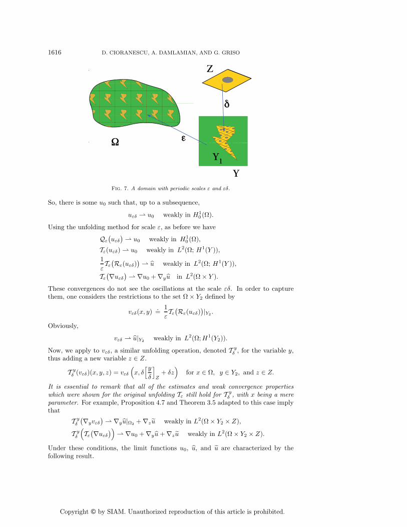
7. Periodic unfolding and multiscales. As we mentioned in the Introduction,the periodic unfolding method turns out to be particularly well-adapted to multiscalesproblems. As an example, we treat here a problem with two different small scales.

Consider two periodicity cells Y and Z, both having the properties introducedat the beginning of section 2 (each associated to its set of periods). Suppose thatY is “partitioned” in two nonempty disjoint open subsets Y1 and Y2, i.e., such thatY1 ∩ Y2 = ∅ and Y = Y 1 ∪ Y 2.

Let Aεδ be a matrix field defined by

Aεδ(x) =

⎧⎪⎪⎨⎪⎪⎩A1

({xε

}Y

)for

{xε

}Y∈ Y1,

A2

({{xε

}Y

δ

}Z

)for

{xε

}Y∈ Y2,

where A1 is in M(α, β, Y1) and A2 in M(α, β, Z) (cf. Definition 5.1). Here we havetwo small scales, namely, ε and εδ, associated, respectively, to the cells Y and Z (seeFigure 7).

Consider the problem∫Ω

Aεδ∇uεδ∇w dx =∫

Ω

f w dx ∀w ∈ H10 (Ω),

with f in L2(Ω). The Lax–Milgram theorem immediately gives the existence anduniqueness of uεδ in H1

0 (Ω) satisfying the estimate

‖uεδ‖H10 (Ω) ≤

1α‖f‖L2(Ω).

Copyright © by SIAM. Unauthorized reproduction of this article is prohibited.

1616 D. CIORANESCU, A. DAMLAMIAN, AND G. GRISO

Z

Y

Y1

Fig. 7. A domain with periodic scales ε and εδ.

So, there is some u0 such that, up to a subsequence,

uεδ ⇀ u0 weakly in H10 (Ω).

Using the unfolding method for scale ε, as before we have

Qε

(uεδ

)⇀ u0 weakly in H1

0 (Ω),

Tε(uεδ) ⇀ u0 weakly in L2(Ω; H1(Y )),1εTε

(Rε(uεδ)

)⇀ u weakly in L2(Ω; H1(Y )),

Tε

(∇uεδ

)⇀ ∇u0 + ∇yu in L2(Ω × Y ).

These convergences do not see the oscillations at the scale εδ. In order to capturethem, one considers the restrictions to the set Ω × Y2 defined by

vεδ(x, y).=

1εTε

(Rε(uεδ)

)|Y2 .

Obviously,

vεδ ⇀ u|Y2 weakly in L2(Ω;H1(Y2)).

Now, we apply to vεδ, a similar unfolding operation, denoted T yδ , for the variable y,

thus adding a new variable z ∈ Z.

T yδ (vεδ)(x, y, z) = vεδ

(x, δ

[yδ

]Z

+ δz)

for x ∈ Ω, y ∈ Y2, and z ∈ Z.

It is essential to remark that all of the estimates and weak convergence propertieswhich were shown for the original unfolding Tε still hold for T y

δ , with x being a mereparameter. For example, Proposition 4.7 and Theorem 3.5 adapted to this case implythat

T yδ

(∇yvεδ

)⇀ ∇yu|Ω2 + ∇z u weakly in L2(Ω × Y2 × Z),

T yδ

(Tε

(∇uεδ

))⇀ ∇u0 + ∇yu+ ∇zu weakly in L2(Ω × Y2 × Z).

Under these conditions, the limit functions u0, u, and u are characterized by thefollowing result.

Copyright © by SIAM. Unauthorized reproduction of this article is prohibited.

THE PERIODIC UNFOLDING METHOD IN HOMOGENIZATION 1617

Theorem 7.1. The functions

u0 ∈ H10 (Ω), u ∈ L2(Ω, H1

per(Y )/R), u ∈ L2(Ω × Ω2, H1per(Z)/R)

are the unique solutions of the variational problem⎧⎪⎪⎪⎪⎪⎪⎪⎨⎪⎪⎪⎪⎪⎪⎪⎩

1|Y ‖Z|

∫Ω

∫Y2

∫Z

A2(z){∇u0 + ∇yu+ ∇z u

}{∇Ψ + ∇yΦ + ∇zΘ

}dx dy dz

+1|Y |

∫Ω

∫Y1

A1(y){∇u0 + ∇yu

}{∇Ψ + ∇yΦ

}dx dy =

∫Ω

f Ψ dx,

∀Ψ ∈ H10 (Ω), ∀Φ ∈ L2(Ω; H1

per(Y )/R), ∀Θ ∈ L2(Ω × Ω2, H1per(Z)/R).

The proof uses test functions of the form

Ψ(x) + εΨ1(x)Φ1

(xε

)+ εδΨ2(x)Φ2

({xε

}Y

)Θ2

(1δ

{xε

}Y

),

where Ψ,Ψ1,Ψ2 are in D(Ω), Φ1 in H1per(Y ), Φ2 ∈ D(Y2), and Θ2 ∈ H1

per(Z).Remark 7.2. The same theorem holds true for a general Aεδ under the hypotheses

Tε(Aεδ) 1Y1 → A1 strongly in [L1(Ω × Y1)]n×n,

T yδ

(Tε(Aεδ) 1Y2

)→ A2 strongly in [L1(Ω × Y2 × Z)]n×n.

Proposition 5.9 (convergence of the energy) and Corollary 5.11 extend withoutany difficulty to the multiscale case.

Proposition 7.3. The convergence for the energy holds true:

limε,δ→0

∫Ω

Aεδ∇uεδ∇uεδ dx

=1

|Y ‖Z|

∫Ω

∫Y2

∫Z

A2(z){∇u0 + ∇yu+ ∇zu

}{∇u0 + ∇yu+ ∇z u

}dx dy dz

+1|Y |

∫Ω

∫Y1

A1(y){∇u0 + ∇yu

}{∇u0 + ∇yu

}dx dy.

Corollary 7.4. The following strong convergences hold true:

T yδ

(∇yvεδ

)⇀ ∇yu|Ω2 + ∇zu strongly in L2(Ω × Y2 × Z),

T yδ

(Tε

(∇uεδ

))⇀ ∇u0 + ∇yu+ ∇z u strongly in L2(Ω × Y2 × Z).

Remark 7.5. A corrector result, similar to that of Theorem 6.1, can be obtained.Remark 7.6. Theorem 7.1 can be extended to the case of any finite number of

distinct scales by a simple reiteration.

8. Further developments. The unfolding method has some interesting prop-erties which make it suitable for more general situations than that presented here. Inproblems which are set on a domain Ωε which depends on the parameter ε, it may bedifficult to have a good notion of convergence for the sequence of solutions uε. Thetraditional way is to extend the solution by 0 outside Ωε; however, this precludes thestrong convergence of these extended functions in general. For the case of holes of the

Copyright © by SIAM. Unauthorized reproduction of this article is prohibited.

1618 D. CIORANESCU, A. DAMLAMIAN, AND G. GRISO

size of order ε distributed ε-periodically, the unfolded sequence lives on a fixed do-main. Similarly, for domains with ε-oscillating boundaries, a partial unfolding yieldsa function which is defined on a fixed domain.

We conclude by giving a list of publications making use of the unfolding methodin several of these directions (both for linear and nonlinear problems).

– Reiterated homogenization: Meunier and Van Schaftingen [56].– Electro-magnetism: Banks et al. [7], Bossavit, Griso, and Miara [15].– Homogenization of thin piezoelectric shells: Ghergu et al. [39].– Homogenization of diffusion deformation media: Griso and Rohan [46].– Homogenization of the Stokes problem in porous media: Cioranescu, Damlamian,

and Griso [25].– Homogenization in perforated domains with Robin boundary conditions: Cio-

ranescu, Donato and Zaki [31], [32].– Homogenization in domains with oscillating boundaries: Damlamian and Pet-

tersson [36].– Homogenization of nonlinear integrals of the calculus of variations: Cioranescu,

Damlamian, and De Arcangelis [27], [28], and [29].– Homogenization of multivalued monotone operators of Leray–Lions type:

Damlamian, Meunier, and Van Schaftingen [37].– Thin junctions in linear elasticity: Blanchard, Gaudiello, and Griso [12], [13],

Blanchard and Griso [14].– Thin domains and free boundary problems arising in lubrication theory:

Bayada, Martin, and Vazquez [9], [10].– Elasticity problems in perforated domains: Griso and Sanchez-Rua [47].– Neumann sieve and Dirichlet shield problems: Onofrei [60], Cioranescu et al.

[26]. This last paper treats the case of domains with ε-periodically distributed “verysmall” holes (their size being a power of ε) on the boundary of which a homogeneousDirichlet condition is prescribed. This requires the introduction of a rescaled unfoldingoperator (which originally appeared in the framework of the two-scale convergence inCasado-Dıaz [20]).

Aknowledgments. We thank Petru Mironescu and Riccardo De Arcangelis forhelpful comments and corrections.

REFERENCES

[1] G. Allaire, Homogenization and two-scale convergence, SIAM J. Math. Anal., 23 (1992),pp. 1482–1518.

[2] G. Allaire and M. Briane, Multiscale convergence and reiterated homogenization, Proc.Roy. Soc. Edinburgh Sect. A, 126 (1996), pp. 297–342.

[3] G. Allaire and C. Conca, Bloch wave homogenization and spectral asymptotic analysis, J.Math. Pures Appl., 2 (1998), pp. 153–208.

[4] G. Allaire, C. Conca, and M. Vanninathan, Spectral asymptotics of the Helmholtz modelin fluid-solid structures, Internat. J. Numer. Methods Engrg., 9 (1999), pp. 1463–1504.

[5] T. Arbogast, J. Douglas, and U. Hornung, Derivation of the double porosity model ofsingle phase flow via homogenization theory, SIAM J. Math. Anal., 21 (1990), pp. 823–836.

[6] J. F. Babadjian and M. Baıa, Multiscale nonconvex relaxation and application to thin films,Asymptot. Anal., 48 (2006), pp. 173–218.

[7] H. T. Banks, V. A. Bokil, D. Cioranescu, N. L. Gibson, G. Griso, and B. Miara,Homogenization of periodically varying coefficients in electromagnetic materials, J. Sci.Comput., 28 (2006), pp. 191–221.

[8] M. Barchiesi, Multiscale homogenization of convex functionals with discontinuous integrand,J. Convex Anal., 14 (2007), pp. 205–226.

Copyright © by SIAM. Unauthorized reproduction of this article is prohibited.

THE PERIODIC UNFOLDING METHOD IN HOMOGENIZATION 1619

[9] G. Bayada, S. Martin, and C. Vazquez, Two-scale homogenization of a hydrodynamicElrod-Adams model, Asymptot. Anal., 44 (2005), pp. 75–110.

[10] G. Bayada, S. Martin, and C. Vazquez, Homogenization of a nonlocal elastohydrodynamiclubrication problem: A new free boundary model, Math. Models Methods Appl. Sci., 15(2005), pp. 1923–1956.

[11] A. Bensoussan, J. L. Lions, and G. Papanicolaou, Asymptotic Analysis for PeriodicStructures, Stud. Math. Appl. 5, North-Holland, Amsterdam, 1978.

[12] D. Blanchard, A. Gaudiello, and G. Griso, Junction of a periodic family of elastic rodswith a 3d plate, Part I, J. Math. Pures Appl., 88 (2007), pp. 1–33.

[13] D. Blanchard, A. Gaudiello, and G. Griso, Junction of a periodic family of elastic rodswith a thin plate, Part II, J. Math. Pures Appl., 88 (2007), pp. 149–190.

[14] D. Blanchard and G. Griso, Microscopic effects in the homogenization of the junction ofrods and a thin plate, Asymptot. Anal., 56 (2008), pp. 1–36.

[15] A. Bossavit, G. Griso, and B. Miara, Modelling of periodic electromagnetic structures:Bianisotropic materials with memory effects, J. Math. Pures Appl., 84 (2005), pp. 819–850.

[16] A. Bourgeat, S. Luckhaus, and A. Mikelic, Convergence of the homogenization processfor a double-porosity model of immiscible two-phase flow, SIAM. J. Math. Anal., 27(1996), pp. 1520–1543.

[17] A. Braides and A. Defranceschi, Homogenization of Multiple Integrals, Oxford Lect. Ser.Math. Appl. 12, Oxford University Press, Oxford, 1998.

[18] A. Braides and D. Lukkassen, Reiterated homogenization of integral functionals, Math.Models Methods Appl. Sci., 10 (2000), pp. 1–25.

[19] D. A. G. Bruggeman, Berechnung verschiedener physikalisher konstanten von heterogenensubstanzen, Ann. Physik., 24 (1935), p. 634.

[20] J. Casado-Dıaz, Two-scale convergence for nonlinear Dirichlet problems in perforated do-mains, Proc. Roy. Soc. Edinburgh Sect. A, 130 (2000), pp. 249–276.

[21] J. Casado-Dıaz and M. Luna-Laynez, A multiscale method to the homogenization of elasticthin reticulated structures, in Homogenization 2001, GAKUTO Internat. Ser. Math. Sci.Appl. 18, Gakkotosho, Tokyo, 2003, pp. 155–168.

[22] J. Casado-Dıaz, M. Luna-Laynez, and J. D. Martın, An adaptation of the multi-scalemethods for the analysis of very thin reticulated structures, C.R. Acad. Sci. Paris, Ser.1, 332 (2001), pp. 223–228.

[23] J. Casado-Dıaz, M. Luna-Laynez, and J. D. Martın, A new approach to the analysis ofthin reticulated structures, in Homogenization 2001, GAKUTO Internat. Ser. Math. Sci.Appl. 18, Gakkotosho, Tokyo, 2003, pp. 257–262.

[24] D. Cioranescu, A. Damlamian, and G. Griso, Periodic unfolding and homogenization,C.R. Acad. Sci. Paris, Ser. 1, 335 (2002), pp. 99–104.

[25] D. Cioranescu, A. Damlamian, and G. Griso, The Stokes problem in perforated domainsby the periodic unfolding method, in Proceedings of the Conference on New Trends inContinuum Mechanics, M. Suliciu, ed., Theta, Bucarest, 2005, pp. 67–80.

[26] D. Cioranescu, A. Damlamian, G. Griso, and D. Onofrei, The periodic unfolding methodfor perforated domains and Neumann sieve models, J. Math. Pures Appl., 89 (2008),pp. 248–277.

[27] D. Cioranescu, A. Damlamian, and R. De Arcangelis, Homogenization of nonlinearintegrals via the periodic unfolding method, C.R. Acad. Sci. Paris, Ser. 1, 339 (2005),pp. 77–82.

[28] D. Cioranescu, A. Damlamian, and R. De Arcangelis, Homogenization of integralswith pointwise gradient constraints via the periodic unfolding method, Ricerche Mat.,55 (2006), pp. 31–54.

[29] D. Cioranescu, A. Damlamian, and R. De Arcangelis, Homogenization of quasiconvexintegrals via the periodic unfolding method, SIAM J. Math. Anal., 37 (2006), pp. 1435–1453.

[30] D. Cioranescu and P. Donato, An Introduction to Homogenization, Oxford Lecture Ser.in Math. Appl. 17, Oxford University Press, Oxford, 1999.

[31] D. Cioranescu, P. Donato, and R. Zaki, The periodic unfolding method in perforateddomains, Port. Math., 63 (2006), pp. 467–496.

[32] D. Cioranescu, P. Donato, and R. Zaki, Asymptotic behavior of elliptic problems inperforated domains with nonlinear boundary conditions, Asymptot. Anal., 53 (2007),pp. 209–235.

[33] G. Dal Maso and A. Defranceschi, Correctors for the homogenization of monotone oper-ators, Differential Integral Equations, 3 (1990), pp. 1151–1166.

Copyright © by SIAM. Unauthorized reproduction of this article is prohibited.

1620 D. CIORANESCU, A. DAMLAMIAN, AND G. GRISO

[34] A. Damlamian, An elementary introduction to periodic unfolding, in Proceedings of theNarvik Conference 2004, GAKUTO Internat. Ser. Math. Sci. Appl. 24, A. Damlamian,D. Lukkassen, A. Meidell, and A. Piatnitski, eds., Gakkotosho, Tokyo, 2006, pp. 119–136.

[35] A. Damlamian and P. Donato, H0-convergence and iterated homogenization, Asymptot.Anal., 39 (2004), pp. 45–60.

[36] A. Damlamian and K. Pettersson, Homogenization of oscillating boundaries, DiscreteContin. Dyn. Syst., 23 (2009), pp. 197–219.

[37] A. Damlamian, N. Meunier, and J. Van Schaftingen, Periodic homogenization of mono-tone multivalued operators, Nonlinear Anal., 67 (2007), pp. 3217–3239.

[38] A. Ene and J. Saint Jean Paulin, On a model of fractured porous media, in MathematicalModelling of Flow Through Porous Media, A. Bourgeat, C. Carasso, S. Luckhaus, andA. Mikelic, eds., World Scientific, River Edge, NJ, 1995, pp. 402–409.

[39] M. Ghergu, G. Griso, H. Mechkour, and B. Miara, Homogenization of thin piezoelectricshells, ESAIM: M2AN Math. Modeling Numer. Anal., 41 (2007), pp. 875–895.

[40] G. Griso, Analyse asymptotique de structures reticulees, These Universite Pierre et MarieCurie (Paris VI), Paris, 1996.

[41] G. Griso, Thin reticulated structures, in Progress in Partial Differential Equations, The MetzSurveys 3, M. Chipot, J. Saint Jean Paulin, and I. Shafrir, eds., Pitman, London, 1994,pp. 161–182.

[42] G. Griso, Error estimate and unfolding for periodic homogenization, Asymptot. Anal., 40(2004), pp. 269–286.

[43] G. Griso, Les methodes d’eclatement en homogeneisation periodique et en elasticitelinearisee, These d’Habilitation, Universite Pierre et Marie Curie, Paris, 2005.

[44] G. Griso, Interior error estimates for periodic homogenization, C.R. Acad. Sci. Paris, Ser.1, 340 (2005), pp. 251–254.

[45] G. Griso, Interior error estimates for periodic homogenization, Anal. Appl., 4 (2006), pp. 61–79.

[46] G. Griso and E. Rohan, On homogenization of diffusion-deformation problem in stronglyheterogeneous media, Ricerche Mat., 56 (2007), pp. 161–188.

[47] G. Griso and T. Sanchez-Rua, Homogenization of an elasticity problem for a catalystsupport by using the unfolding method, submitted.

[48] M. Lenczner, Homogeneisation d’un circuit electrique, C.R. Acad. Sci. Paris, Ser. 2, 324(1997), pp. 537–542.

[49] M. Lenczner and D. Mercier, Homogenization of periodic electrical networks includingvoltage to current amplifiers, SIAM Multiscale Model. Simul., 2 (2004), pp. 359–397.

[50] M. Lenczner and G. Senouci-Bereksi, Homogenization of electrical networks includingvoltage-to-voltage amplifiers, Math. Models Methods Appl. Sci., 9 (1999), pp. 899–932.

[51] M. Lenczner, M. Kader, and P. Perrier, Modele a deux echelles de l’equation des ondesa coefficients oscillants, C.R. Acad. Sci. Paris, Ser. 1, 328 (2000), pp. 335–340.

[52] J. L. Lions, D. Lukkassen, L. E. Persson, and P. Wall, Reiterated homogenization ofmonotone operators, Chinese Ann. Math. Ser. B, 22 (2001), pp. 1–12.

[53] D. Lukkassen, Reiterated homogenization of non-standard Lagrangians, C.R. Acad. Sci.Paris, Ser. 1, 332 (2001), pp. 999–1004.

[54] D. Lukkassen and G. W. Milton, On hierarchical structures and reiterated homogenization,in Proceedings of the Conference on Function Spaces, Interpolation Theory and RelatedTopics in Honor of Jack Peetre on his 65th Birthday, M. Cwikwl, M. Englis, A. Kufner,L.-E. Persson, and G. Sparr, eds, Walter de Gruyter, Berlin, 2002, pp. 311–324.

[55] D. Lukkassen, G. Nguetseng, and P. Wall, Two-scale convergence, Int. J. Pure Appl.Math., 2 (2002), pp. 35–86.

[56] N. Meunier and J. Van Schaftingen, Periodic reiterated homogenization for elliptic func-tions, J. Math. Pures Appl., 9 (2005), pp. 1716–1743.

[57] G. Milton, The Theory of Composites, Cambridge University Press, Cambridge, 2002.[58] G. Nguetseng, A general convergence result for a functional related to the theory of homog-

enization, SIAM J. Math. Anal., 20 (1989), pp. 608–629.[59] O. A. Oleinik, A. S. Shamaev, and G. A. Yosifian, Mathematical Problems in Elasticity

and Homogenization, North-Holland, Amsterdam, 1992.[60] D. Onofrei, The unfolding operator near a hyperplane and its applications to the Neumann

sieve model, Adv. Math. Sci. Appl., 16 (2006), pp. 239–258.