The Peierls-Nabarro model as a limit of a Frenkel-Kontorova model

arX

iv:1

010.

0865

v1 [

mat

h.A

P] 5

Oct

201

0

The Peierls-Nabarro model as a limit of a

Frenkel-Kontorova model

A. Z. Fino∗, a, d, H. Ibrahima, b, R. Monneau∗∗, c

January 3, 2014

Abstract

We study a generalization of the fully overdamped Frenkel-Kontorova model in dimension n ≥ 1. This model

describes the evolution of the position of each atom in a crystal, and is mathematically given by an infinite

system of coupled first order ODEs. We prove that for a suitable rescaling of this model, the solution converges

to the solution of a Peierls-Nabarro model, which is a coupled system of two PDEs (typically an elliptic PDE

in a domain with an evolution PDE on the boundary of the domain). This passage from the discrete model to

a continuous model is done in the framework of viscosity solutions.

MSC: 49L25; 30E25Keywords: Frenkel-Kontorova, Peierls-Nabarro, viscosity solutions, dislocations, discrete-continuous, boundary con-

ditions.

1 Introduction

In this paper we are interested in two models describing the evolution of defects in crystals, calleddislocations. These two models are the Frenkel-Kontorova model and the Peierls-Nabarro model. TheFrenkel-Kontorova model is a discrete model which describes the evolution of the position of atoms ina crystal. On the contrary, the Peierls-Nabarro model is a continuous model where the dislocation isseen as a phase transition. The main goal of the paper is to show rigorously how the Peierls-Nabarromodel can be obtained as a limit of the Frenkel-Kontorova model after a suitable rescaling.

1.1 Peierls-Nabarro model

Let us start to present the Peierls-Nabarro model. We set

Ω = x = (x1, ..., xn) ∈ Rn, xn > 0,

∗Departement de Mathematiques, Laboratoire de mathematiques appliquees, UMR CNRS 5142, Universite de Pau

et des Pays de l’Adour, 64000 Pau, France. E-mail: [email protected], Lebanese University, P.O. Box 37 Tripoli, Lebanon.∗∗Invited professor at LaMA-Liban, Lebanese University, P.O. Box 37 Tripoli, Lebanon.bLebanese University, Faculty of Sciences, Mathematics Department, Hadeth, Beirut, Lebanon. E-mail:

[email protected] Paris-Est, CERMICS, Ecole des Ponts, 6 et 8 avenue Blaise Pascal, Cite Descartes Champs-sur-Marne,

77455 Marne-la-Vallee Cedex 2, France. E-mail: [email protected] Departement de Mathematiques, Universite de La Rochelle, 17042 La Rochelle, France.

1

and for a time 0 < T ≤ +∞, we look for solutions u0 of the following system with β ≥ 0:

βu0t (x, t) = ∆u0(x, t) (x, t) ∈Ω× (0, T )

u0t (x, t) = F (u0(x, t)) +∂u0

∂xn(x, t) (x, t) ∈ ∂Ω× (0, T ),

(1.1)

where the boundary ∂Ω is defined by:

∂Ω = x = (x1, ..., xn) ∈ Rn, xn = 0,

and the unknown u0(x, t) ∈ R is a scalar-valued function with the initial data

u0(x, 0) = u0(x) for

x ∈ Ω := ∂Ω ∪ Ω if β > 0

x ∈ ∂Ω if β = 0.(1.2)

We assume the following conditions on the function F : R → R and on the initial data u0 :

F ∈W 2,∞(R) and

u0 ∈W 3,∞(Ω) if β > 0

u0 ∈W 3,∞(∂Ω) if β = 0.(1.3)

For simplicity we have taken a high regularity on the initial data, but this condition can be weaken.The classical Peierls-Nabarro model corresponds to the case β = 0 with a 1-periodic function F (seeSection 2). For a derivation and study of the Peierls-Nabarro model, we refer the reader to [22] (and[30, 28] for the original papers and [29] for a recent review by Nabarro on the Peierls-Nabarro model).Let us mention that a physical and numerical study of the evolution problem (1.1) has been treatedin [27].

In this paper we consider the general case β ≥ 0, since the case β = 0 is natural in the Frenkel-Kontorova model (see Section 2), and mathematically the case β > 0 is easier to study. In the specialcase β = 0, this problem can be reformulated (at least at a formal level) as a nonlocal evolutionequation written on ∂Ω in any dimension. See in particular [18] for such a reformulation in dimensionn = 2 and a limit of the Peierls-Nabarro model to the discrete dislocation dynamics (see also [26] fora homogenization result of the Peierls-Nabarro model). We refer the reader to [10] for the study ofstationary solutions of our model when F = −W ′.

1.2 Frenkel-Kontorova model

We now present the Frenkel-Kontorova model. This is a discrete model which contains a small scaleε > 0 that can be seen as the order of the distance between atoms. We set the discrete analogue ofΩ:

Ωε = (εZ)n−1 × ε(N \ 0)with discrete boundary

∂Ωε = (εZ)n−1 × 0,and we set

Ωε= Ωε ∪ ∂Ωε.

We look for solutions uε(x, t) with x ∈ Ωε, t ≥ 0, of the following system for β ≥ 0:

βuεt (x, t) = ∆ε[uε](x, t), (x, t) ∈Ωε × (0, T )

uεt (x, t) = F (uε(x, t)) +Dε[uε](x, t), (x, t) ∈ ∂Ωε × (0, T ),(1.4)

2

with initial data

uε(x, 0) = u0(x) for

x ∈ Ω

εif β > 0

x ∈ ∂Ωε if β = 0,(1.5)

where we have used the following notation for the discrete analogue of ∆ and ∂∂xn

respectively:

∆ε[uε](x, t) =1

ε2

∑

y∈Zn, |y|=1

(uε(x+ εy, t)− uε(x, t))

Dε[uε](x, t) =1

ε

∑

y∈Zn, |y|=1, yn≥0

(uε(x+ εy, t)− uε(x, t)).

(1.6)

In this model, the function uε(x, t) describes the scalar analogue of the position of the atom of index xin the crystal. The classical fully overdamped Frenkel-Kontorova model is a one dimensional model.It corresponds to the particular case n = 2 where uε(x, t) = 0 if x ∈ Ωε, and therefore only theuε(εx, t) for x ∈ Z × 0 can be non trivial (we refer the reader to [9]). Remark that in the caseβ > 0, we can consider classical solutions using the Cauchy-Lipschitz theory, while at least in thecase β = 0, it is convenient to deal with viscosity solutions (see Section 3).

More generally, Frenkel-Kontorova are also used for the description of vacancy defects at equi-libruim, see [20]. See also [19], where the authors study the problem involving a dislocation insidethe interphase between two identical lattices. Their model corresponds to our model (1.4) at theequilibrium with F = −W ′ where the potential W is a cosine function. For other 2D FK models, see[12, 13]. For homogenization results of some FK models, we refer the reader to [17].

1.3 Main result

Our main result is the following theorem which establishes rigorously (for the first time up to ourknowledge) the link between the two famous physical models: the Frenkel-Kontorova model and thePeierls-Nabarro model.

Theorem 1.1 (Existence, uniqueness and convergence)Let ε > 0, β ≥ 0 and 0 < T ≤ +∞. Under the condition (1.3) there exists a unique discrete viscositysolution uε of (1.4)-(1.5). Moreover, as ε → 0, the sequence uε converges to the unique boundedviscosity solution u0 of (1.1)-(1.2). The convergence uε → u0 has to be understood in the followingsense: for any compact set K ⊂ Ω× [0, T ), we have:

‖uε − u0‖L∞(K∩(Ωε×[0,T ))) → 0 as ε→ 0.

A formal version of this result has been announced in [16]. We refer the reader to Section 3 forthe definition of viscosity solutions. The proof of convergence is done in the framework of viscositysolutions, using the half-relaxed limits. The uniqueness of the limit u0 follows from a comparisonprinciple that we prove for (1.1), using in particular a special test function introduced by Barles in[5]. Most of the difficulties arise here from the unboundedness of the domain, and in the non standardcase β = 0, where the evolution equation is on the boundary of the domain instead of being in theinterior of the domain. Let us notice that because system (1.4) can be seen as a discretization schemeof system (1.1), then Theorem 1.1 can be interpreted as a convergence result for such a scheme. Inthe literature on numerical analysis of finite difference schemes, we find other results of convergencefor different equations (see for instance [8] and [7]). Let us mention that an estimate on the rate ofconvergence of uε to u0 is still an open question for our system.

3

Remark 1.2 From the proof of Theorem 1.1, it is easy to see that the result still holds true if Fis replaced by a sequence (F ε)ε of functions which converges in W 2,∞(R). For such an example ofapplication, see (2.3) at the end of Section 2; see also [16].

1.4 Organization of the paper

This paper is organized as follows. In Section 2, we present the physical motivation to our problem.In Section 3, we present the definitions of viscosity solutions for the discrete and continuous problem(1.4)-(1.5) and (1.1)-(1.2) respectively. Section 4 is dedicated to construct uniform barriers of thesolution uε of (1.4)-(1.5). Using those barriers, we prove in Section 5 the existence of a solution forthe discrete problem (1.4)-(1.5). Section 6 is devoted to the proof of Theorem 1.1. Sections 7 and 8are respectively devoted to the proofs of the comparison principle for the discrete problem (1.4)-(1.5)and the continuous problem (1.1)-(1.2), that were presented in Section 3 and used in the whole paper.Finally, in the Appendix, we give a convenient corollary of Ishii’s lemma, that we use in Section 8.

2 Physical motivation

2.1 Geometrical description

We start to call (e1, e2, e3) an orthonormal basis of the three dimensional space. In the correspondingcoordinates, we consider a three-dimensional crystal where each atom is initially at the position of anode I of the lattice

Λ = Z2 ×

(1

2+ Z

).

This lattice is simply obtained by a translation along the vector 12e3 of the lattice Z3, and will be

more convenient for the derivation of our model. We assume that each atom I ∈ Λ of the crystal hasthe freedom to move to another position I + uIe2 where uI ∈ R is a unidimensional displacement.In particular, we will be able to describe dislocations only with Burgers vectors that are multiplesof the vector e2 (see [22] for an introduction to dislocations and a definition of the Burgers vector).Moreover we introduce the general notation

I = (I ′,−I3) for all I = (I ′, I3) ∈ Z2 ×

(1

2+ Z

)with I ′ = (I1, I2) ∈ Z

2

and will only consider antisymmetric displacements uI , i.e. satisfying

uI = −uI for all I ∈ Λ. (2.1)

We also introduce the discrete gradient

(∇du)I =

uI+e1 − uIuI+e2 − uIuI+e3 − uI

.

Generally, the core of a dislocation is localized where the discrete gradient is not small. In our model,screw and edge dislocations will be represented as follows.

4

Screw dislocationFor I = (I1, I2, I3), we can consider a dislocation line parallel to the vector e2, with a displacementuI independent on I2, i.e. such that uI = s(I1, I3). We will assume for instance that

s(I1,+12 ) = −s(I1,−1

2) → 0 as I1 → −∞

s(I1,+12 ) = −s(I1,−1

2) → 12 as I1 → +∞.

Moreover, if there is no applied stress on the crystal, then it is reasonable to assume that

dist((∇du)I ,Z

3)→ 0 as |(I1, I3)| → +∞

which means that the crystal is perfect far from the core of the dislocation.Edge dislocationFor I = (I1, I2, I3), we can consider a dislocation line parallel to the vector e1, with a displacementuI independent on I1, i.e. uI = e(I2, I3). We will assume for instance that

e(I2,+12 ) = −e(I2,−1

2 ) → 0 as I2 → −∞

e(I2,+12 ) = −e(I2,−1

2 ) → 12 as I2 → +∞.

Moreover, if there is no applied stress on the crystal, then it is reasonable to assume that

dist((∇du)I ,Z

3)→ 0 as |(I2, I3)| → +∞.

Remark that this model can also describe more generally curved dislocations, which are neither screw,nor edge, but are mixed dislocations.

2.2 Energy of the crystal

We assume that each atom I is related to its nearest neighbors J by a nonlinear spring, whose force isderived from a smooth potentialWIJ . Then formally the full energy of the crystal after a displacementu = (uI)I∈Λ is

E(u) =1

2

∑

I,J∈Λ, |I−J|=1

WIJ(uI − uJ).

We assume that the dislocation cores are only included in the double plane I3 = ±12 . We also assume

that

WIJ(a) =

εW (a) if |I3| = |J3| = 1

2W (a) if |I3| 6= 1

2 or |J3| 6= 12 .

Here ε > 0 is a small parameter. This means that the springs lying between the two planes I3 = ±12

are very weak in comparison to the other springs. This will allow the core of the dislocation to spreadout on the lattice as ε→ 0 and will allow us to recover the Peierls-Nabarro model in this limit, aftera suitable rescaling.

Notice that, to be compatible with the antisymmetry (2.1) of the crystal, it is reasonable toassume that

W (−a) =W (a) for all a ∈ R.

Recall that each line of atoms I0 + Ze2 only contains atoms of identical nature (i.e. surrounded bya similar configuration of springs). Therefore for uI = s(I1, I3), a lattice of atoms at the position

5

I + uIe2 and another lattice of atoms at the position I + uIe2 + k(I1,I3)e2 with arbitrary k(I1,I3) ∈ Z

are completely equivalent. Therefore their energy should be the same, and it is then natural toassume that the potential W is 1-periodic, i.e. satisfies

W (a+ 1) =W (a) for all a ∈ R.

We will also assume that non-deformed lattices minimize globally their energy, i.e. satisfy

W (Z) = 0 and W > 0 on R\Z.

Let us now assume that a constant global shear stress is applied on the crystal such that it createsa global shear of the crystal in the direction e2 with respect to the coordinate I3. This means thatthere exists a constant τ ∈ R such that

dist((∇du)I − τe3,Z

3)→ 0

as I goes far away from the core of the dislocation. Remark that this assumption is compatible withthe antisymmetry (2.1) of u. If there is no dislocations, we can simply take for instance uI = τI3.

2.3 Fully overdamped dynamics of the crystal

The natural dynamics should be given by Newton’s law satisfied by each atom. This dynamics is veryrich and for certain shear stress τ , it is known (see [14, 21]) in 2D lattices that certain edge dislocationscan propagate with constant mean velocity. This is due to the fact that part of the energy is lost byradiation of sound waves in the crystal. This phenomenon is similar to the effective drag force createdby the surrounding fluid on a boat or an air plane. The resulting behaviour is a kind of dissipativedynamics that we modelise here by a fully overdamped dynamics of the crystal. See [23, 25, 24])for a fundamental justification of overdamped type dynamics based on explicit computations in a1D Hamiltonian model. For general physical justifications of the dissipative effects in the motion ofdislocations, see also [22, 1].

We recall that we assume that the dislocation cores are only contained in the double plane I3 = ±12 .

For this reason, we will artificially distinguish the dynamics inside this double plane and outside thisdouble plane. We consider the following fully overdamped dynamics (where the velocity of each atomis proportional to the force deriving from the energy) which is written formally as:

αI uI = −∇uIE(u) with αI =

1 if |I3| = 1

2α if |I3| 6= 1

2 ,(2.2)

for some constant α ≥ 0. Here uI denotes the time derivative of the displacement uI and

∇uIE(u) :=

∑

J∈Λ, |J−I|=1

W ′IJ(uI − uJ).

Remark in particular that this dynamics preserves the antisymmetry (2.1) of u. For slow motion ofdislocations (i.e. small velocity with respect to the velocity of sound in the crystal), it is reasonableto assume that α = 0, i.e. the lattice is instantaneously at the equilibrium outside the double planeI3 = ±1

2 .We also assume that the potential is harmonic close to its minima, i.e. satisfies

W (a) =a2

2for |a| ≤ δ <

1

2

6

and assume that the strain is small enough in the crystal outside the double plane I3 = ±12 , i.e. we

assume that

|uJ − uI | ≤ δ for any J, I ∈ Λ such that |J − I| = 1 and |I3| 6=1

2or |J3| 6=

1

2.

This assumption allows us, in the region I3 6= ±12 , to consider forces that can be expressed linearly

in terms of the displacement. We also set

τ = εσ for some σ ∈ R and vI = uI − εσI3.

Using the antisymmetry of the solution (2.1), we deduce that we can rewrite the dynamics (2.2) withα = 0 as

0 =∑

J∈Λ, |J−I|=1

(vJ − vI) for I3 >1

2

vI = εσ − εW ′(2vI + εσ) +∑

J∈Λ, |J−I|=1, J3≥1

2

(vJ − vI) for I3 =1

2.

Then we see that

uε(x, t) = v(xε+ 1

2)

(t

ε

)

solves (1.4) with β = 0 and F replaced by

F ε(a) = σ −W ′(2a+ εσ). (2.3)

Remark 2.1 At the level of modeling, we could also consider more general lattices than Zn with

more general nearest neighbors interactions, but this case is not covered by the result of Theorem 1.1and would require a specific work.

3 Viscosity solutions

In this section we present the notion of viscosity solutions and some of their properties for thediscrete problem (1.4)-(1.5) and then for the continuous problem (1.1)-(1.2). For the classical notionof viscosity solutions, we refer the reader to [3], [4], [15].

3.1 Viscosity solutions for the discrete problem

Before stating the definition of viscosity solutions for the discrete problem (1.4)-(1.5), we start bydefining some terminology. Let ε, δ > 0 and 0 < T ≤ +∞. Given a point P0 = (x0, t0) ∈ Ω

ε × [0, T ),the set N ε

δ (t0) ⊂ Ωε × [0, T ) is defined by:

N εδ (P0) = P = (y, t) ∈ Ω

ε × [0, T ); |y − x0| ≤ ε and |t− t0| < δ. (3.1)

The spaces USC(Ωε × [0, T )) and LSC(Ω

ε × [0, T )) are defined respectively by:

USC(Ωε × [0, T )) = u defined on Ω

ε × [0, T ); ∀x ∈ Ωε, u(x, · ) ∈ USC([0, T )) (3.2)

7

andLSC(Ω

ε × [0, T )) = u defined on Ωε × [0, T ); ∀x ∈ Ω

ε, u(x, · ) ∈ LSC([0, T )), (3.3)

where USC([0, T )) (resp. LSC([0, T ))) is the set of locally bounded upper (resp. lower) semi-continuous functions on [0, T ). In a similar manner, we define the space Ck(Ω

ε × [0, T )), k ∈ N,by:

Ck(Ωε × [0, T )) = u defined on Ω

ε × [0, T ); ∀x ∈ Ωε, u(x, · ) ∈ Ck([0, T )). (3.4)

Next, given β ≥ 0, we present the following definition:

Definition 3.1 (Viscosity sub/super solutions)1. Viscosity sub-solutions. A function u ∈ USC(Ω

ε× [0, T )) is a viscosity sub-solution of problem(1.4)-(1.5) provided that:

(i) u(x, 0) ≤ u0(x) for

x ∈ Ω

εif β > 0

x ∈ ∂Ωε if β = 0,

(ii) for any ϕ ∈ C1(Ωε×[0, T )), if u−ϕ has a zero local maximum at a point P0 = (x0, t0) ∈ Ω

ε×[0, T )(i.e. ∃ δ > 0 such that ∀P ∈ N ε

δ (P0), we have (u− ϕ)(P ) ≤ (u− ϕ)(P0) = 0) then

βϕt(P0) ≤ ∆ε[ϕ](P0)

∣∣∣∣for P0 ∈ Ωε × (0, T ) if β > 0for P0 ∈ Ωε × [0, T ) if β = 0

ϕt(P0) ≤ F (ϕ(P0)) +Dε[ϕ](P0) for P0 ∈ ∂Ωε × (0, T ).(3.5)

2. Viscosity super-solutions. A function u ∈ LSC(Ωε × [0, T )) is a viscosity super-solution of

problem (1.4)-(1.5) provided that:

(i) u(x, 0) ≥ u0(x) for

x ∈ Ω

εif β > 0

x ∈ ∂Ωε if β = 0,

(ii) for any ϕ ∈ C1(Ωε×[0, T )), if u−ϕ has a zero local minimum at a point P0 = (x0, t0) ∈ Ω

ε×[0, T )(i.e. ∃ δ > 0 such that ∀P ∈ N ε

δ (P0), we have (u− ϕ)(P ) ≥ (uε − ϕ)(P0) = 0) then

βϕt(P0) ≥ ∆ε[ϕ](P0)

∣∣∣∣for P0 ∈ Ωε × (0, T ) if β > 0for P0 ∈ Ωε × [0, T ) if β = 0

ϕt(P0) ≥ F (ϕ(P0)) +Dε[ϕ](P0) for P0 ∈ ∂Ωε × (0, T ).(3.6)

3. Viscosity solutions. A function u ∈ C0(Ωε× [0, T )) is a viscosity solution of problem (1.4)-(1.5)

if it is a viscosity sub- and super-solution of (1.4)-(1.5).

Definition 3.2 We say that u is a viscosity sub-solution (resp. super-solution) of (1.4) if u onlysatisfies (ii) in the Definition 3.1.

Remark 3.3 Note that a function u is a viscosity subsolution of (1.4) if it satisfies the viscosityinequalities on Ω

ε × (0, T ) if β > 0 and on(Ωε × (0, T )

)∪ (Ωε × 0) if β = 0.

Theorem 3.4 (Comparison principle in the discrete case)Let u ∈ USC(Ω

ε×[0, T )) (resp. v ∈ LSC(Ωε×[0, T ))) be a viscosity sub-solution (resp. super-solution)

for the problem (1.4)-(1.5) where 0 < T <∞, such that ‖u‖L∞(Ωε×[0,T )), ‖v‖L∞(Ω

ε×[0,T )) < +∞. Then

u(x, t) ≤ v(x, t) for all (x, t) ∈ Ωε × [0, T ).

Theorem 3.4 will be proved in Section 7.

8

3.2 Viscosity solutions for the continuous problem

Similarly as in subsection 3.1 we denote by USC(Ω × [0, T )) (resp. LSC(Ω × [0, T ))) the set oflocally bounded upper (resp. lower) semi-continuous functions on Ω × [0, T ). We also denote byCk(Ω× [0, T )) the classical set of continuously k-differentiable functions on Ω× [0, T ).

Definition 3.5 (Viscosity sub/super solutions)1. Viscosity sub-solutions. A function u ∈ USC(Ω× [0, T )) is a viscosity sub-solution of problem(1.1)-(1.2) provided that:

(i) u ≤ u0 on

Ω× 0 if β > 0

∂Ω × 0 if β = 0.

(ii) for any ϕ ∈ C2(Ω× [0, T )), if u−ϕ has a zero local maximum at a point P0 = (x0, t0) ∈ Ω× [0, T )then

βϕt(P0) ≤ ∆ϕ(P0)

∣∣∣∣for P0 ∈ Ω× (0, T ) if β > 0for P0 ∈ Ω× [0, T ) if β = 0

min

βϕt(P0)−∆ϕ(P0) , ϕt(P0)− F (ϕ(P0))−

∂ϕ

∂xn(P0)

≤ 0 for P0 ∈ ∂Ω× (0, T ).

(3.7)2. Viscosity super-solutions. A function u ∈ LSC(Ω × [0, T )) is a viscosity super-solution ofproblem (1.1)-(1.2) provided that:

(i) u ≥ u0 on

Ω× 0 if β > 0

∂Ω × 0 if β = 0.

(ii) for any ϕ ∈ C2(Ω× [0, T )), if u−ϕ has a zero local minimum at a point P0 = (x0, t0) ∈ Ω× [0, T )then

βϕt(P0) ≥ ∆ϕ(P0)

∣∣∣∣for P0 ∈ Ω× (0, T ) if β > 0for P0 ∈ Ω× [0, T ) if β = 0

max

βϕt(P0)−∆ϕ(P0) , ϕt(P0)− F (ϕ(P0))−

∂ϕ

∂xn(P0)

≥ 0 for P0 ∈ ∂Ω× (0, T ).

(3.8)3. Viscosity solutions. A function u ∈ C0(Ω× [0, T )) is a viscosity solution of problem (1.1)-(1.2)if it is a viscosity sub- and super-solution of (1.1)-(1.2).

Theorem 3.6 (Comparison principle in the continuous case)Let u ∈ USC(Ω×[0, T )) (resp. v ∈ LSC(Ω× [0, T ))) be a viscosity sub-solution (resp. super-solution)of problem (1.1)-(1.2) where 0 < T <∞, such that ‖u‖L∞(Ω×[0,T )), ‖v‖L∞(Ω×[0,T )) < +∞. Then

u ≤ v on Ω× [0, T )

This theorem will be proved in section 8.

Remark 3.7 Remark that in the case β = 0, the problem can be reformulated (at least for smoothsolutions) as a nonlocal evolution equation written on the boundary ∂Ω. See for instance the work[11] on the relation bewteen fractional Laplacian and harmonic extensions. Note that there is also aviscosity theory for nonlocal operators (see [6]).

4 Construction of barriers

This section is devoted to the construction of barriers for the solution uε of (1.4)-(1.5) for all β ≥ 0.

9

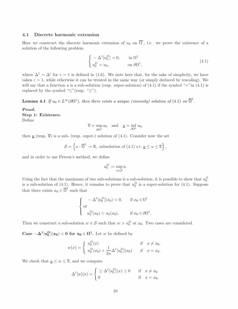
4.1 Discrete harmonic extension

Here we construct the discrete harmonic extension of u0 on Ωε, i.e. we prove the existence of a

solution of the following problem

−∆1[uD0 ] = 0, in Ω1

uD0 = u0, on ∂Ω1,(4.1)

where ∆1 = ∆ε for ε = 1 is defined in (1.6). We note here that, for the sake of simplicity, we havetaken ε = 1, while otherwise it can be treated in the same way (or simply deduced by rescaling). Wewill say that a function u is a sub-solution (resp. super-solution) of (4.1) if the symbol “=”in (4.1) isreplaced by the symbol “≤”(resp. “≥”).

Lemma 4.1 If u0 ∈ L∞(∂Ω1), then there exists a unique (viscosity) solution of (4.1) on Ω1.

Proof.Step 1: Existence.Define

u = sup∂Ω1

u0 and u = inf∂Ω1

u0,

then u (resp. u) is a sub- (resp. super-) solution of (4.1). Consider now the set

S =u : Ω

1 → R, subsolution of (4.1) s.t. u ≤ u ≤ u,

and in order to use Perron’s method, we define

uD0 := supu∈S

u.

Using the fact that the maximum of two sub-solutions is a sub-solution, it is possible to show that uD0is a sub-solution of (4.1). Hence, it remains to prove that uD0 is a super-solution for (4.1). Suppose

that there exists x0 ∈ Ω1such that

−∆1[uD0 ](x0) < 0, if x0 ∈Ω1

or

uD0 (x0) < u0(x0), if x0 ∈∂Ω1.

Then we construct a sub-solution w ∈ S such that w > uD0 at x0. Two cases are considered.

Case −∆1[uD0](x0) < 0 for x0 ∈ Ω1. Let w be defined by

w(x) =

uD0 (x) if x 6= x0,

uD0 (x0) +1

2n∆1[uD0 ](x0) if x = x0.

We check that u ≤ w ≤ u, and we compute

∆1[w](x) =

≥ ∆1[uD0 ](x) ≥ 0 if x 6= x0

0 if x = x0,

10

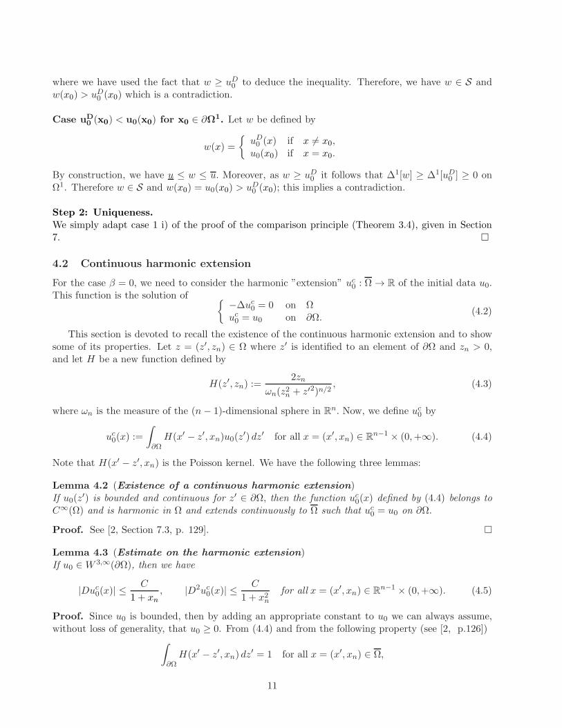
where we have used the fact that w ≥ uD0 to deduce the inequality. Therefore, we have w ∈ S andw(x0) > uD0 (x0) which is a contradiction.

Case uD0(x0) < u0(x0) for x0 ∈ ∂Ω1. Let w be defined by

w(x) =

uD0 (x) if x 6= x0,u0(x0) if x = x0.

By construction, we have u ≤ w ≤ u. Moreover, as w ≥ uD0 it follows that ∆1[w] ≥ ∆1[uD0 ] ≥ 0 onΩ1. Therefore w ∈ S and w(x0) = u0(x0) > uD0 (x0); this implies a contradiction.

Step 2: Uniqueness.We simply adapt case 1 i) of the proof of the comparison principle (Theorem 3.4), given in Section7.

4.2 Continuous harmonic extension

For the case β = 0, we need to consider the harmonic ”extension” uc0 : Ω → R of the initial data u0.This function is the solution of

−∆uc0 = 0 on Ωuc0 = u0 on ∂Ω.

(4.2)

This section is devoted to recall the existence of the continuous harmonic extension and to showsome of its properties. Let z = (z′, zn) ∈ Ω where z′ is identified to an element of ∂Ω and zn > 0,and let H be a new function defined by

H(z′, zn) :=2zn

ωn(z2n + z′2)n/2, (4.3)

where ωn is the measure of the (n− 1)-dimensional sphere in Rn. Now, we define uc0 by

uc0(x) :=

∫

∂ΩH(x′ − z′, xn)u0(z

′) dz′ for all x = (x′, xn) ∈ Rn−1 × (0,+∞). (4.4)

Note that H(x′ − z′, xn) is the Poisson kernel. We have the following three lemmas:

Lemma 4.2 (Existence of a continuous harmonic extension)If u0(z

′) is bounded and continuous for z′ ∈ ∂Ω, then the function uc0(x) defined by (4.4) belongs toC∞(Ω) and is harmonic in Ω and extends continuously to Ω such that uc0 = u0 on ∂Ω.

Proof. See [2, Section 7.3, p. 129].

Lemma 4.3 (Estimate on the harmonic extension)If u0 ∈W 3,∞(∂Ω), then we have

|Duc0(x)| ≤C

1 + xn, |D2uc0(x)| ≤

C

1 + x2nfor all x = (x′, xn) ∈ R

n−1 × (0,+∞). (4.5)

Proof. Since u0 is bounded, then by adding an appropriate constant to u0 we can always assume,without loss of generality, that u0 ≥ 0. From (4.4) and from the following property (see [2, p.126])

∫

∂ΩH(x′ − z′, xn) dz

′ = 1 for all x = (x′, xn) ∈ Ω,

11

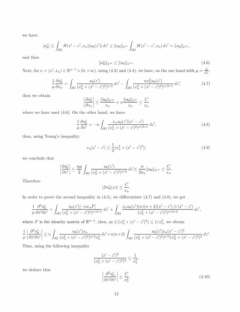
we have:

|uc0| ≤∫

∂ΩH(x′ − z′, xn)|u0(z′)| dz′ ≤ ‖u0‖L∞

∫

∂ΩH(x′ − z′, xn) dz

′ = ‖u0‖L∞ ,

and then‖uc0‖L∞ ≤ ‖u0‖L∞ . (4.6)

Next, for x = (x′, xn) ∈ Rn−1×(0,+∞), using (4.3) and (4.4), we have, on the one hand with µ = 2

ωn:

1

µ

∂uc0∂xn

=

∫

∂Ω

u0(z′)

(x2n + (x′ − z′)2)n/2dz′ −

∫

∂Ω

nx2nu0(z′)

(x2n + (x′ − z′)2)n/2+1dz′, (4.7)

then we obtain ∣∣∣∣∂uc0∂xn

∣∣∣∣ ≤‖u0‖L∞

xn+ n

‖u0‖L∞

xn≤ C

xn

where we have used (4.6). On the other hand, we have:

1

µ

∂uc0∂x′

= −n∫

∂Ω

xnu0(z′)(x′ − z′)

(x2n + (x′ − z′)2)n/2+1dz′, (4.8)

then, using Young’s inequality:

xn|x′ − z′| ≤ 1

2(x2n + (x′ − z′)2), (4.9)

we conclude that∣∣∣∣∂uc0∂x′

∣∣∣∣ ≤nµ

2

∫

∂Ω

u0(z′)

(x2n + (x′ − z′)2)n/2dz′≤ n

2xn‖u0‖L∞ ≤ C

xn.

Therefore

|Duc0(x)| ≤C

xn.

In order to prove the second inequality in (4.5), we differentiate (4.7) and (4.8), we get

1

µ

∂2uc0∂x′∂x′

=

∫

∂Ω

u0(z′)[−nxnI ′]

(x2n + (x′ − z′)2)n/2+1dz′ +

∫

∂Ω

xnu0(z′)(n)(n+ 2)(x′ − z′)⊗ (x′ − z′)

(x2n + (x′ − z′)2)n/2+2dz′,

where I ′ is the identity matrix of Rn−1, then, as 1/(x2n + (x′ − z′)2) ≤ 1/x2n, we obtain

1

µ

∣∣∣∣∂2uc0∂x′∂x′

∣∣∣∣ ≤ n

∫

∂Ω

u0(z′)xn

(x2n + (x′ − z′)2)n/2x2ndz′+n(n+2)

∫

∂Ω

u0(z′)xn(x

′ − z′)2

(x2n + (x′ − z′)2)n/2(x2n + (x′ − z′)2)2dz′.

Thus, using the following inequality

(x′ − z′)2

(x2n + (x′ − z′)2)2≤ 1

x2n,

we deduce that ∣∣∣∣∂2uc0∂x′∂x′

∣∣∣∣ ≤C

x2n. (4.10)

12

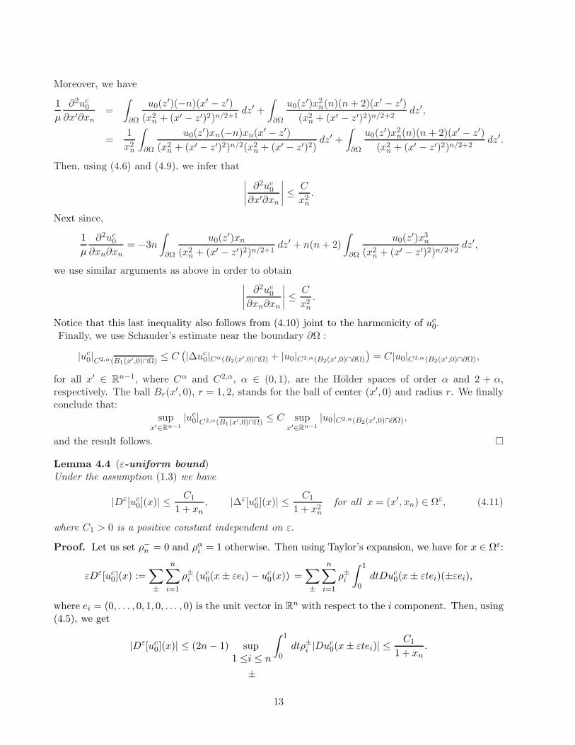
Moreover, we have

1

µ

∂2uc0∂x′∂xn

=

∫

∂Ω

u0(z′)(−n)(x′ − z′)

(x2n + (x′ − z′)2)n/2+1dz′ +

∫

∂Ω

u0(z′)x2n(n)(n+ 2)(x′ − z′)

(x2n + (x′ − z′)2)n/2+2dz′,

=1

x2n

∫

∂Ω

u0(z′)xn(−n)xn(x′ − z′)

(x2n + (x′ − z′)2)n/2(x2n + (x′ − z′)2)dz′ +

∫

∂Ω

u0(z′)x2n(n)(n + 2)(x′ − z′)

(x2n + (x′ − z′)2)n/2+2dz′.

Then, using (4.6) and (4.9), we infer that∣∣∣∣∂2uc0∂x′∂xn

∣∣∣∣ ≤C

x2n.

Next since,

1

µ

∂2uc0∂xn∂xn

= −3n

∫

∂Ω

u0(z′)xn

(x2n + (x′ − z′)2)n/2+1dz′ + n(n+ 2)

∫

∂Ω

u0(z′)x3n

(x2n + (x′ − z′)2)n/2+2dz′,

we use similar arguments as above in order to obtain∣∣∣∣∂2uc0

∂xn∂xn

∣∣∣∣ ≤C

x2n.

Notice that this last inequality also follows from (4.10) joint to the harmonicity of uc0.Finally, we use Schauder’s estimate near the boundary ∂Ω :

|uc0|C2,α(B1(x′,0)∩Ω) ≤ C(|∆uc0|Cα(B2(x′,0)∩Ω) + |u0|C2,α(B2(x′,0)∩∂Ω)

)= C|u0|C2,α(B2(x′,0)∩∂Ω),

for all x′ ∈ Rn−1, where Cα and C2,α, α ∈ (0, 1), are the Holder spaces of order α and 2 + α,

respectively. The ball Br(x′, 0), r = 1, 2, stands for the ball of center (x′, 0) and radius r. We finally

conclude that:sup

x′∈Rn−1

|uc0|C2,α(B1(x′,0)∩Ω) ≤ C supx′∈Rn−1

|u0|C2,α(B2(x′,0)∩∂Ω),

and the result follows.

Lemma 4.4 (ε-uniform bound)Under the assumption (1.3) we have

|Dε[uc0](x)| ≤C1

1 + xn, |∆ε[uc0](x)| ≤

C1

1 + x2nfor all x = (x′, xn) ∈ Ωε, (4.11)

where C1 > 0 is a positive constant independent on ε.

Proof. Let us set ρ−n = 0 and ραi = 1 otherwise. Then using Taylor’s expansion, we have for x ∈ Ωε:

εDε[uc0](x) :=∑

±

n∑

i=1

ρ±i (uc0(x± εei)− uc0(x)) =∑

±

n∑

i=1

ρ±i

∫ 1

0dtDuc0(x± εtei)(±εei),

where ei = (0, . . . , 0, 1, 0, . . . , 0) is the unit vector in Rn with respect to the i component. Then, using

(4.5), we get

|Dε[uc0](x)| ≤ (2n− 1) sup1 ≤i ≤ n

±

∫ 1

0dtρ±i |Duc0(x± εtei)| ≤

C1

1 + xn.

13

Then, in order to terminate the proof, it is sufficient to write ∆ε[uD0 ] using Taylor’s expansion as

ε2∆ε[uc0](x) :=∑

±

n∑

i=1

(uc0(x± εei)− uc0(x))

=∑

±

n∑

i=1

(±εei∇uc0(x) +

∫ 1

0dt

∫ t

0dsD2uc0(x± εsei)(±εei)(±εei)

)

= ε2∑

±

n∑

i=1

∫ 1

0dt

∫ t

0dsD2uc0(x± εsei) · (ei, ei).

(4.12)

Thus, thanks to (4.5), we finally obtain:

|∆ε[uc0](x)| ≤ 2n sup1 ≤i ≤ n

±

∫ 1

0dt

∫ t

0ds|D2uc0(x± εsei)| ≤

C1

1 + x2n,

and the proof is done.

4.3 Uniform barriers for β ≥ 0

In this subsection, we show uniform barriers for the solution uε of (1.4)-(1.5) for all β ≥ 0 in thespecial case where u0 = uc0.

Proposition 4.5 (Uniform barriers in ε for all β ≥ 0 for u0 = uc0)Under assumption (1.3), there exists a constant C > 0 independent on ε > 0, β ≥ 0 and T such thatif

u+(x, t) := uc0(x) +C(√1 + xn − 1 + t)

u−(x, t) := uc0(x)−C(√1 + xn − 1− t)

∣∣∣∣ for (x, t) ∈ Ωε × [0, T ), (4.13)

then u+ (resp. u−) is a supersolution (resp. subsolution) of (1.4)-(1.5). However, if uε is a boundedviscosity solution of (1.4)-(1.5), then we have

u− ≤ uε ≤ u+ on Ωε × [0, T ), (4.14)

and moreover:|uε(x, t)| ≤ ‖u0‖L∞ + t‖F‖L∞ for (x, t) ∈ Ω

ε × [0, T ).

Proof.Step 1: sub/supersolution propertyWe first check that u+ is a super-solution of (1.4)-(1.5). Indeed,• If (x, t) ∈ Ω

ε × 0, then u+(x, t) ≥ uc0(x) = u0(x).• If (x, t) ∈ ∂Ωε × (0, T ), then we take C > 0 such that

C ≥ F (u+(x, t)) +Dε[uc0](x) + CDε[√1 + xn] ⇐⇒ u+t (x, t) ≥ F (u+(x, t)) +Dε[u+](x, t).

Using the fact that Dε[√1 + xn](xn = 0) ≤ 1

2 , we see that such a constant C exists.• If (x, t) ∈ Ωε × [0, T ), then we can use Lemma 4.4. We get

∆ε[uc0](x) ≤C1

1 + x2n≤ C

4(1 + xn)3/2,

14

where the last inequality is true for C > 0 large enough. Moreover, by repeating the same computa-tions as in (4.12), we easily get with f(a) =

√1 + a:

∆ε[√1 + xn] =

∫ 1

0dt

∫ t

0ds∑

±

f ′′(xn ± εs) ≤∫ 1

0dt

∫ t

0ds.2.f ′′(xn) ≤ f ′′(xn) = − 1

4(1 + xn)3/2,

(4.15)where we have used the concavity of the function f ′′. Then we have

∆ε[uc0](x) ≤C

4(1 + xn)3/2≤ −C∆ε[

√1 + xn],

henceβu+t (x, t) = βC ≥ 0 ≥ ∆ε[u+](x, t).

As a consequence, we finally deduce that u+ is a super-solution. In a similar way, by taking inaddition the following assumption on C :

C ≥ −F (u−(x, t)) −Dε[uc0](x) + CDε[√1 + xn]

we can prove that u− is a sub-solution.

Step 2: bounds on uε

Let us call v(x, t) := ‖u0‖L∞ + t‖F‖L∞ . It is easy to check that v is a super-solution of (1.4)-(1.5).Then

min(u+, v)

is still a super-solution and is bounded. Therefore, if uε is a bounded viscosity solution of (1.4)-(1.5),we can then apply the comparison principle (Theorem 3.4) to conclude that

uε ≤ min(u+, v).

This shows the upper bounds. For the lower bounds, we proceed similarly with max(u−,−v).

4.4 Barriers for β > 0

We have the following

Proposition 4.6 (Barriers for β > 0)Under the assumptions of Theorem 1.1, for every β > 0, there exists a constant Cβ > 0 such that forall ε, if uε is a bounded viscosity solution of (1.4)-(1.5), then we have

|uε(x, t) − u0(x)| ≤ tCβ for (x, t) ∈ Ωε × [0, T ).

Proof.Using in particular the fact that F is bounded and that u0 ∈ W 2,∞(Ω), we simply check thatu0(x) + tCβ is a super-solution for a suitable constant Cβ> 0 and apply the comparison principle.We proceed similarly for sub-solutions u0(x)− tCβ.

15

5 Existence and uniqueness of a solution for the discrete problem

The aim of this section is to prove the existence of solutions of problem (1.4)-(1.5). Cauchy-Lipschitzmethod is the main tool used to prove the existence of solutions for β > 0, while in the case β = 0we need barriers to prove the existence.

Theorem 5.1 (Existence and uniqueness, β > 0)If u0 and F satisfy (1.3) and β > 0, then there exists a unique bounded solution uβ,ε ∈ C1(Ω

ε× [0, T ))of problem (1.4)-(1.5).

Proof. The proof is done using the classical Cauchy-Lipschitz theorem. Let B := L∞(Ωε) be the

Banach space with the norm

‖u‖B := supx∈Ω

ε|u(x)|, for every u ∈ B,

and F : B −→ B be the map defined, for every u ∈ B and x ∈ Ωε, by

F [u](x) :=

1

β∆ε[u](x), x ∈ Ωε,

F (u(x)) +Dε[u](x), x ∈ ∂Ωε

where ∆ε[u](x) and Dε[u](x) are defined as in (1.6), dropping the variable t on both sides of (1.6).Then, for every u, v ∈ B and x ∈ Ω

ε, we have two cases; either x ∈ Ωε, and hence we obtain

‖F [u](x)−F [v](x)‖B ≤ ‖ 1β∆ε[u− v](x)‖B

≤ 4n

βε2‖u− v‖B ,

or x ∈ ∂Ωε, then:

‖F [u](x)−F [v](x)‖B ≤ ‖Dε[u− v](x) + |F (u(x))− F (v(x))|‖B≤

(2(2n − 1)

ε+ ‖F ′‖L∞(R)

)‖u− v‖B .

In all cases we conclude that F is globally Lipschitz continuous. By the Cauchy-Lipschitz theorem,we get the existence and uniqueness of a solution uβ,ε ∈ C1(Ω

ε × [0, T )) satisfying

uβ,εt (·, t) = F [uβ,ε](·, t),

such that uβ,ε(· , 0) = u0(· ).

Theorem 5.2 (Existence and uniqueness, β = 0)If u0 and F satisfy (1.3) and β = 0, then there exists a unique bounded continuous solution u0,ε onΩε × [0, T ) of the problem (1.4)-(1.5).

Proof. We consider the solution uβ,ε given by Theorem 5.1 for the choice u0 = uc0. Let

u = lim supβ→0

∗uβ,ε and u = lim infβ→0

∗uβ,ε.

16

Then, using Propositon 4.5, we obtain

u− ≤ u ≤ u ≤ u+ and |u|, |u| ≤ ‖u0‖L∞ + t‖F‖L∞ . (5.1)

Using standard arguments similar to those in Step 1.1 of the proof of Theorem 1.1 in Section 6, wecan show that u (resp. u) is a super- (resp. sub-) solution of the problem (1.4). The only difficulty isto recover the viscosity inequality on Ωε × 0. This last inequality follows from the fact that uβ,ε isa classical solution and then satisfies the equation also at t = 0. Finally, using (5.1), we deduce thatu (resp. u) is a super- (resp. sub-) solution of the problem (1.4)-(1.5). Then the comparison principle(Theorem 3.4) implies that u ≤ u. So u = u =: u0,ε is a continuous bounded solution of (1.4)-(1.5).The uniqueness of this solution follows again from the comparison principle.

As a conclusion, there exists a unique (viscosity) solution uε ∈ C0(Ωε × [0, T )) of problem (1.4)-

(1.5) defined by:

uε :=

uβ,ε if β > 0,

u0,ε if β = 0.

(5.2)

Remark 5.3 The existence of a solution could also be proven by Perron’s method.

6 Proof of Theorem 1.1

This section is devoted to the proof of Theorem 1.1. Note that in the sequel, we use the followingnotation:

ΩT := Ω× (0, T ), ∂lΩT := ∂Ω × (0, T ), ΩT := Ω× [0, T ),

andΩεT := Ωε × (0, T ), ∂lΩε

T := ∂Ωε × (0, T ), ΩεT := Ω

ε × [0, T ),

where ∂l denotes the lateral boundary.

Proof of Theorem 1.1. The proof is divided into two steps.

Step 1: u and u are, respectively, sub- and super-solution of (1.1)-(1.2).

Let uε be the bounded viscosity solution of the problem (1.4)-(1.5). We define, for (x, t) ∈ ΩT , thefunctions u and u as follows:

u(x, t) := lim supy → x, s→ t, ε→ 0

y ∈ Ωε

, s ∈ [0, T )

uε(y, s) and u(x, t) := lim infy → x, s→ t, ε→ 0

y ∈ Ωε

, s ∈ [0, T )

uε(y, s). (6.1)

We start by showing that u is a viscosity sub-solution of (1.1)-(1.2).

Step 1.1: Proof of 1 (ii) in Definition 3.5.

Let ϕ ∈ C2(ΩT ) and P0 = (x0, t0) ∈ ΩT such that u − ϕ has a zero local maximum at P0. Withoutloss of generality, we can assume that this maximum is global and strict. Therefore we have

∀r > 0, ∃δ = δ(r) > 0 such that ϕ− u ≥ δ > 0 in ΩT \Br(P0), (6.2)

17

where Br(P0) ⊂ Rn ×R is the open ball of radius r and of center P0. Now, let w

ε := ϕ− uε for someε > 0. Then, using the definition of u, and inequality (6.2), we infer that

wε ≥ δ

2in Ω

εT \Br(P0), (6.3)

for all r > 0 and for ε > 0 small enough. Using [4, Lemma 4.2], it is then classical to see that thereexists a sequence P ∗

ε = (x∗ε, t∗ε) ∈ Ω

εT ∩Br(P0) such that, as ε→ 0, we have

P ∗ε → P0, uε(P ∗

ε ) → u(P0) and uε − ϕ has a local maximum at P ∗ε . (6.4)

Two cases are then considered.

Case 1 : P0 ∈ Ω × [0, T ). We argue by contradiction. Assume that there exists a positive constantγ > 0 such that

βϕt(P0) = ∆ϕ(P0) + γ

∣∣∣∣for P0 ∈ Ω× (0, T ) if β > 0for P0 ∈ Ω× [0, T ) if β = 0

(6.5)

Moreover, using (6.4) and the fact that uε is a viscosity sub-solution of problem (1.4)-(1.5), weconclude that

βϕt(P∗ε ) ≤ ∆ε[ϕ](P ∗

ε ), (6.6)

and by Taylor’s expansion, this inequality (6.6) implies

βϕt(P∗ε ) ≤ ∆ϕ(P ∗

ε ) + oε(1). (6.7)

Combining (6.5) and (6.7) yields:

γ ≤ −β(ϕt(P∗ε )− ϕt(P0)) + ∆ϕ(P ∗

ε )−∆ϕ(P0) + oε(1),

where the right hand side goes to zero as ε→ 0. This contradicts the fact that γ > 0.

Case 2 : P0 ∈ ∂lΩT . We repeat similar arguments as in Case 1. Suppose that

min

βϕt(P0)−∆ϕ(P0) , ϕt(P0)− F (ϕ(P0))−

∂ϕ

∂xn(P0)

= γ1 > 0. (6.8)

Inequality (6.8) impliesβϕt(P0)−∆ϕ(P0) ≥ γ1, (6.9)

and

ϕt(P0)− F (ϕ(P0))−∂ϕ

∂xn(P0) ≥ γ1. (6.10)

On the one hand, if P ∗ε ∈ Ωε

T , then, using (6.7) and (6.9), we obtain a contradiction by using thesame reasoning as in Case 1. On the other hand, if P ∗

ε ∈ ∂lΩεT , then using (6.4) and the fact that uε

is a subsolution of (1.4)-(1.5) we obtain:

ϕt(P∗ε ) ≤ F (ϕ(P ∗

ε )) +Dε[ϕ](P ∗ε ),

and then, using Taylor’s expansion, we obtain

ϕt(P∗ε ) ≤

∂ϕ

∂xn(P ∗

ε ) + F (ϕ(P ∗ε )) +O(ε).

18

Finally, subtracting this inequality from (6.10), we conclude, after passing to the limit as ε→ 0, thatγ1 ≤ 0; contradiction.

Step 1.2 : Proof of 1(i) in Definition 3.5.

From Propositions 4.5 and 4.6, we can pass to the limit and get from the barriers

|u(x, t)− u0(x)| ≤tCβ if β > 0C(t+

√1 + xn − 1) if β = 0 and u0 = uc0

∣∣∣∣ for all (x, t) ∈ ΩT .

Therefore for t = 0 we recover 1(i) in Definition 3.5 for all β ≥ 0.

Step 2: Existence and convergence.

From Step 1 we conclude that u is a viscosity sub-solution of (1.1)-(1.2) and by a similar manner, wecan show that u is a viscosity super-solution of (1.1)-(1.2). Moreover u and u are bounded, becauseProposition 4.5 implies

|u|, |u| ≤ ‖u0‖L∞ + t‖F‖L∞

Then by the comparison principle for problem (1.1)-(1.2) (Theorem 3.6), we have u ≤ u. On theother hand, by the definition of u and u, we have u ≤ u. As a consequence, we deduce, for (x, t) ∈ ΩT ,that:

u(x, t) = u(x, t) = limε→0,y→x,s→t

uε(y, s) =: u0(x, t) (6.11)

where u0 is then a continuous viscosity solution of problem (1.1)-(1.2). Moreover u0 is unique, still bythe comparison principle. Finally, we also observe that the convergence uε → u0 as ε → 0 is locallyuniform in the following sense:

‖uε − u0‖L∞(K∩ ΩεT ) −→ 0 as ε→ 0,

for any compact set K ⊂ ΩT . Indeed, suppose that there exists θ > 0 such that for all k > 0 thereexists εk satisfying 0 < εk <

1k with

‖uεk − u0‖L∞(K∩(Ωεk×[0,T ))) > θ.

Then, there exists a sequence Pk ∈ K ∩ (Ωεk × [0, T )) such that

|uε(Pk)− u0(Pk)| > θ. (6.12)

Now, since K∩(Ωεk × [0, T )) ⊂ K with K compact, there exists a subsequence, denoted for simplicity

by Pk, such that Pk → P∞ as k → ∞. Finally, taking the lim infk→∞,Pk→P∞in the inequality (6.12)

and using (6.11), we obtain 0 > θ which gives a contradiction.

6.1 Other barriers and comments on another possible approach for β = 0

Let us notice that for β = 0, we have natural barriers for the ε-problem, which are:

uD,ε0 (x)± Cεt

where uD,ε0 = uD0 is the discrete harmonic extension (we make its dependence explicit on ε) associated

to the operator ∆ε, and with the constant Cε satisfying

Cε ≥ Dε[uD,ε0 ] + ‖F‖L∞ .

19

Then another possible approach to show the convergence of uε to u0, could be to control the solutionas ε goes to zero, showing that:1) the constant Cε can be taken independent on ε (using the regularity of u0 on ∂Ω).2) the discrete harmonic extension uD,ε

0 converges to the continuous harmonic extension uc0 as ε tendsto zero.Then we could also introduce a (more classical) notion of viscosity solution in the case β = 0, assumingthat at t = 0, we can compare the sub/super-solution to the initial data (taken to be equal to theharmonic extension uD,ε

0 for the ε-problem and uc0 for the limit problem). Nevertheless, this otherapproach would require some additional work (to show 1) and 2)), and would not simplify the proofs.

Remark 6.1 (Convergence of the discrete harmonic extension to the continuous har-monic extension)Notice that point 2) is a consequence of our convergence theorem (Theorem 1.1) in the case β = 0.Indeed, in the case β = 0, the bounded solutions satisfy

|uε(x, t)− uD,ε0 (x)| ≤ Cεt

and thenuε(x, 0) = uD,ε

0 (x).

On the other hand, the functionsuc0(x)± C0t

are barriers for the limit problem if

C0 ≥ ‖∂uc0

∂n‖L∞ + ‖F‖L∞ .

Then bounded solutions of the continuous problem satisfy

|u0(x, t)− uc0(x)| ≤ C0t

and thenu0(x, 0) = uc0(x).

Finally from the (locally uniform) convergence of uε to u0 in particular for t = 0, we deduce that uD,ε0

converges, locally uniformly, to uc0.

7 Proof of Theorem 3.4

In order to emphasize the main points, we perform the proof in several steps.

Step 1: Rescaling. We want to reduce the problem (1.4)-(1.5) to the case ε = 1 and with anonlinearity F replaced by a monotone one. To this end, we introduce the new functions

u(x, t) := e−λtu(εx, εt), v(x, t) := e−λtv(εx, εt), (x, t) ∈ Ω1 × [0, T ),

where T = T/ε and λ > 0 is a constant to be determined later. We see easily that u (resp. v) is asub-solution (resp. super-solution) of the following problem

βut = ∆1[u]− βλu in Ω1 × (0, T ),

ut = F (u, t) +D1[u] on ∂Ω1 × (0, T ),

(7.1)

20

and

u(x, 0) = u0(εx) for

x ∈ Ω

1if β > 0

x ∈ ∂Ω1 if β = 0,(7.2)

withβ = εβ and F (u, t) = εe−λtF (eλtu)− λu.

We argue by contradiction assuming that

M := supΩ

1×[0,T )

(u− v) > 0.

From the definition ofM, there exists a sequence P k = (xk, tk) ∈ Ω1×[0, T ) such that u(P k)−v(P k) →

M > 0 as k → ∞. Let us choose an index k0 such that

u(P k0)− v(P k0) ≥ M

2.

At this stage, if we write x = (x′, xn) with x′ = (x1, . . . , xn−1), we define

Ψ(x, t, s) :=|t− s|2

2δ+

η

T − t+ α|x′|2 + γ

√1 + xn, (x, t, s) ∈ Ω

1 × [0, T )2,

where δ, η, α, γ > 0 will be chosen later, and we consider

M :=Mδ,η,α,γ := supx∈Ω

1,t,s∈[0,T )

(u(x, t) − v(x, s)−Ψ(x, t, s)). (7.3)

Step 2: A priori estimates. Now, if we choose η, α, γ such that:

η

T − tk0+ α|(xk0)′|2 + γ

√1 + xk0n ≤ M

4,

we conclude that

M ≥ u(P k0)− v(P k0)−Ψ(xk0 , tk0 , tk0) ≥ M

4> 0.

Moreover, from the definition of M , there exists (x, t, s) ∈ Ω1 × [0, T )2 such that

u(x, t)− v(x, s)−Ψ(x, t, s) =M > 0 (7.4)

and|t− s|2

2δ+

η

T − t+ α|x′|2 + γ

√1 + xn ≤ C (7.5)

whereC = ‖u‖

L∞(Ω1×[0,T ))

+ ‖v‖L∞(Ω

1×[0,T ))

.

Step 3: Getting contradiction. In this step, we have to distinguish two cases:

Case 1. (t > 0 and s > 0)

In this case, we have two sub-cases:(i) If x ∈ Ω1. From the definition of (x, t, s), we see that

u(x, t) ≤ ϕu(x, t) :=M + v(x, s) + Ψ(x, t, s).

21

Even if u has not the required regularity, we see by a simple approximation argument that we canchoose

ϕu(x, t) = u(x, t) for x 6= x.

Then ϕu is a test function for u at (x, t) and we deduce the following viscosity inequality

βη

(T − t)2+ β

(t− s)

δ≤ ∆1[u](x, t)− βλu(x, t). (7.6)

Similarly, we havev(x, s) ≥ ϕv(x, s) := −M + u(x, t)−Ψ(x, t, s),

and we chooseϕv(x, s) = v(x, s) for x 6= x.

We then get the viscosity inequality

β(t− s)

δ≥ ∆1[v](x, s)− βλv(x, s). (7.7)

Subtracting the two viscosity inequalities and setting w(x) = u(x, t)− v(x, s), we get

0 ≤ βη

(T − t)2≤ ∆1[w](x)− βλw(x)

≤ ∆1[M +Ψ(· , t, s)](x)≤ α

∑

|y−x|=1,y∈Zn

(|y′|2 − |x′|2) + γ∑

|y−x|=1,y∈Zn

(√

1 + yn −√1 + xn) =: A+B,

where in the second line we have used the fact that w(y)−Ψ(y, t, s) ≤M for all y ∈ Ω1with equality

for y = x. Remark that, B = γζ(xn) with, for a ≥ 1,

ζ(a) = f(a+ 1) + f(a− 1)− 2f(a) with f(a) =√1 + a,

hence we get as in (4.12) or (4.15)

ζ(a) =∑

±

∫ 1

0dt

∫ t

0dsf ′′(a± s) ≤ f ′′(a)

where we have used the concavity of f ′′. Using moreover the a priori estimate (7.5) we have√1 + xn ≤

C/γ, and we deduce that

B ≤ −C ′γ4 with C ′ =1

4C3.

On the other hand, we have

A = α∑

|y−x|=1,y∈Zn

(y′ − x′)(y′ + x′) ≤ 2nα(1 + 2|x′|) ≤ 2n(α+ 2√α√C), (7.8)

where we have used the a priori estimate (7.5) (α|x′|2 ≤ C). Finally, if we take α, γ small enough sothat 2n(α + 2

√α√C) < C ′γ4, we conclude that 0 ≤ A+B < 0, and hence a contradiction.

22

(ii) If x ∈ ∂Ω1. This is a similar case of the latter one where we use the same arguments. After thesame choice of the test function, we arrive at

η

(T − t)2+t− s

δ≤ F (u(x, t), t) +D1[u](x, t), (7.9)

andt− s

δ≥ F (v(x, s), s) +D1[v](x, s). (7.10)

Subtracting (7.9) and (7.10), we infer that

η

(T − t)2≤ γ(

√2− 1) +

∑

|y−x|=1,y∈Zn,yn≥xn

α(|y′|2 − |x′|2) + [F (u(x, t), t)− F (v(x, s), s)]

≤ γ +∑

|y−x|=1,y∈Zn

α(|y′|2 − |x′|2) + [F (u(x, t), t)− F (u(x, t), s)]

+ [F (u(x, t), s)− F (v(x, s), s)]. (7.11)

Now, if we take λ ≥ ε‖F ′‖L∞(R), we get F′u ≤ 0 and

F (u(x, t), s)− F (v(x, s), s) ≤ 0, (7.12)

thanks to the fact that u(x, t)− v(x, s) ≥ 0. Moreover, as |F t| ≤ C0 = C0(ε, λ, ‖F‖W 1,∞(R)), we get

|F (u(x, t), t)− F (u(x, t), s)| ≤ C0|t− s| ≤ C0

√2Cδ, (7.13)

where we have used the a priori estimate (7.5) (|t− s|2/(2δ) ≤ C). Now, substituting (7.8), (7.12)and (7.13) into (7.11), we infer that

0 <η

(T − t)2≤ 2n(α+ 2

√α√C) + γ + C0

√2Cδ.

Finally, for η > 0 fixed, we get a contradiction by choosing δ, α and γ small enough.

Case 2. (t = 0 or s = 0)

For η, α, γ fixed, we assume that there exists a sequence δ → 0 and (x, t, s) = (xδ, tδ, sδ) ∈ Ω

1× [0, T )2

such that tδ= 0 or sδ = 0. We deal with the case t

δ= 0 as the other case sδ = 0 is similar. Then

u(xδ, 0) − v(xδ, sδ) =M +Ψ(xδ, 0, s) ≥ M

4> 0.

From (7.5), we deduce that, up to an extraction of a subsequence, we have (xδ, sδ) → (x, 0) ∈Ω1 × [0, T ) as δ → 0. Therefore for β > 0 we have

0 <M

4≤ lim sup

δ→0(u(xδ, 0)− v(xδ, sδ)) ≤ u(x, 0)− v(x, 0) ≤ 0,

where we have used the comparison to the initial condition. This leads to a contradiction in the caseβ > 0 or β = 0 and x ∈ ∂Ω1. For the case β = 0 and x ∈ Ω1, we get a contradiction exactly as incase 1 i).

It is worth noticing that, in the whole proof, we first fix η, and then we choose respectively γ, αand δ small enough.

23

8 Proof of Theorem 3.6

In this section we first present the construction of an auxiliary function ξ which plays a crucial rolein the proof of Theorem 3.6.

Lemma 8.1 (Auxiliary function)Let u ∈ USC(Ω × [0, T )), v ∈ LSC(Ω × [0, T )) such that u ≤ C0, v ≥ −C0, C0 ≥ 0, and letM := supΩ×[0,T )(u− v) > 0. Then for all c > 0, there exists a C∞-function ξc : R

n × [0, T ) → R with

|ξc| ≤ 3C0 and a positive constant ac > 0 such that for every x, y ∈ Ω and s, t ∈ [0, T ) :

v(y, s) ≤ ξc

(x+ y

2,t+ s

2

)≤ u(x, t),

if u(x, t)− v(y, s) ≥M − ac, |x− y|+ |t− s| ≤ ac and |x|, |y| ≤ c.

Proof. We essentially revisit the proof of Lemma 5.2 in Barles [5]. Without loss of generality, we canextend the proof of our result on [0, T ] by defining the end point of u and v as follows:

u(x, T ) = lim supt < T, (y, t) → (x, T )

u(y, t), v(x, T ) = lim inft < T, (y, t) → (x, T )

v(y, t).

Let M := supB2c×[0,T ](u− v) with B2c :=x ∈ Ω; |x| ≤ 2c

Let F = (x, t) ∈ B2c × [0, T ]; u(x, t) −

v(x, t) =M. We have u ≤ C0, v ≥ −C0 and u− v =M on F . This implies that

|u|, |v| ≤ C0 +M ≤ 3C0 on F . (8.1)

Moreover it is easy to check that F is a closed subset of B2c × [0, T ] and that the restriction of u andv to F are continuous. Therefore, the restriction to F of the function (x, t) 7→ (u + v)/2 is also acontinuous function on F which satisfies (8.1). We may extend this function as a continuous functionin R

n × R (still bounded by 3C0) and then, by standard regularization arguments, there exists aC∞-function ξ such that

∣∣∣∣ξ(x, t)−u(x, t) + v(x, t)

2

∣∣∣∣ ≤M

8on F and |ξ| ≤ 3C0 on R

n × R. (8.2)

In order to show the lemma, we now argue by contradiction assuming that there exist two sequences(xac , tac), (yac , sac) such that for ac small enough, u(xac , tac)− v(yac , sac) ≥M − ac and |xac − yac |+|tac −sac | ≤ ac and such that, say, u(xac , tac)− ξ

(xac + yac

2,tac + sac

2

)< 0. Extracting, if necessary,

subsequences, we may assume without loss of generality that (xac , tac), (yac , sac) → (x, t). Then itis easy to show the convergence of u(xac , tac) − v(yac , sac) to M = u(x, t) − v(x, t). By consideringthe upper semi-continuity of u and the lower semi-continuity of v, this implies, on the one hand,u(xac , tac) → u(x, t), v(yac , sac) → v(x, t). On the other hand, by using the continuity of ξ, we obtain

u(x, t)− ξ(x, t) = limac→0

(u(xac , tac)− ξ

(xac + yac

2,tac + sac

2

))≤ 0. (8.3)

But since u(x, t)− v(x, t) =M, with (x, t) ∈ F , we deduce from (8.2) that

ξ(x, t) ≤ u(x, t) + v(x, t)

2+M

8= u(x, t)− 3M

8< u(x, t),

24

which contradicts (8.3). Finally, we arrive to the result by taking ξc as the restriction of ξ on [0, T )multiplied by a cut-off function ψ ∈ C∞(Rn) such that ψ = 1 on Bc and zero outside B2c.

Proof of Theorem 3.6. The proof is divided into three steps.Step 1: Test function. In order to replace the nonlinearity F by a monotone one, we define the newfunctions

u := e−λtu and v := e−λtv,

where λ > 0 is a constant which will be determined later. Obviously, u (resp. v) is a sub-solution(resp. super-solution) of the following problem

βut = ∆[u]− βλu in Ω× (0, T ),

ut =∂u

∂xn+ F (u, t) on ∂Ω× (0, T ),

(8.4)

and

u(x, 0) = u0(x) for

x ∈ Ω if β > 0

x ∈ ∂Ω if β = 0,(8.5)

withF (u, t) = e−λtF (eλtu)− λu.

Let us assume that M := supΩ×[0,T )(u− v) > 0 and let us exhibit a contradiction. By the definition

of the supremum, there exists P k0 = (xk0 , tk0) ∈ Ω× [0, T ), for some index k0, such that

u(P k0)− v(P k0) ≥ M

2. (8.6)

Let us introduce the following constant:

C∗ = ‖u‖L∞(Ω×[0,T )) + ‖v‖L∞(Ω×[0,T )).

We now take the following notation: x = (x′, xn) with x′ = (x1, . . . , xn−1), and for α, γ, η > 0 (to be

fixed later), we can approximate the functions u, v by the functions:

u(x, t) := u(x, t)− α|x′|2 − γ√1 + xn − η

T − t≤ C∗, (8.7)

v(y, s) := v(y, s) + α|y′|2 + γ√

1 + yn +η

T − s≥ −C∗ (8.8)

and defineM := sup

x∈Ω,t∈[0,T )

(u(x, t)− v(x, t)).

In order to dedouble the variables in space and time, following the proof of Theorem 3.2 in [5], wedefine the function Φ : (Ω× [0, T ))2 → R by:

Φ(x, t, y, s) :=(x− y)2

ε2+B(xn − yn)

2

ε2+

(t− s)2

δ2+

2(t− s)(xn − yn)

δ2

−(xn − yn)F

(ξ

(x+ y

2,t+ s

2

),t+ s

2

),

25

where the parameters B, ε, δ > 0 will be chosen later. Moreover c > 0 is a constant that will bedefined later (only depending on α, γ, λ,C∗, ‖F‖L∞(R)) and the smooth function

ξ = ξc (8.9)

is the auxiliary function associated to u and v, and given by Lemma 8.1, which shows in particularthe following estimate

|ξ| ≤ 3C∗ (8.10)

We note that Φ(x, t, x, t) = 0. Then we set

M =MB,ε,δ := supx,y∈Ω, t,s∈[0,T )

(u(x, t)− v(y, s)− Φ(x, t, y, s)) ≥ M. (8.11)

Step 2: A priori estimates. By choosing η, α, γ small enough such that

η

T − tk0+ α|(xk0)′|2 + γ

√1 + xk0n ≤ M

8,

it follows from (8.6) that

M ≥ M ≥ u(P k0)− v(P k0) ≥ M

4> 0. (8.12)

Hence, from the definition of M, there exist sequences xk, yk ∈ Ω, tk, sk ∈ [0, T ) such that

u(xk, tk)− v(yk, sk)− Φ(xk, t

k, yk, sk) −→M > 0 as k → ∞,

and, by taking k large enough, we deduce that

u(xk, tk)− v(yk, sk)− Φ(xk, t

k, yk, sk) ≥ M

2> 0. (8.13)

From (8.10), it follows that

|F (ξ(xk + yk

2,tk+ sk

2),tk+ sk

2)| ≤ C1 = C1(λ,C∗, ‖F‖L∞(R)).

Then if we take ε ≤ δ ≤ 1, Young’s inequality yields

|(xkn − ykn)F (ξ(xk + yk

2,tk+ sk

2),tk+ sk

2)| ≤ (xkn − ykn)

2

ε2+C21ε

2

4≤ (xkn − ykn)

2

ε2+C21δ

2

4, (8.14)

and|2(tk − sk)(xkn − ykn)|

δ2≤ 1

2

(tk − sk)2

δ2+ 2

(xkn − ykn)2

ε2. (8.15)

Using (8.14), (8.15), we deduce that for B ≥ 3

Φ(xk, tk, yk, sk) ≥ (x− y)2

ε2+

(B − 3)(xn − yn)2

ε2+

(t− s)2

2δ2− C2

1δ2

4≥ −C

21δ

2

4.

Using (8.13), we conclude that

(xk − yk)2

ε2+

(tk − sk)2

2δ2+ α(|(xk)′|2 + |(yk)′|2) + γ

√1 + xkn + γ

√1 + ykn +

η

T − tk+

η

T − sk≤ C∗∗,

26

with (for δ ≤ 1)

C∗∗ = C∗ +C21

4= C∗∗(λ,C∗, ‖F‖L∞(R)).

Then, up to an extraction of a subsequence, we have

(xk, tk, yk, sk) → (x, t, y, s) ∈ (Ω)2 × [0, T )2 as k → ∞,

with

u(x, t)− v(y, s)− Φ(x, t, y, s) =M > 0 and Φ(x, t, y, s) ≥ −C21δ

2

4(8.16)

and the same a priori estimate

(x− y)2

ε2+

(t− s)2

2δ2+ α(|x′|2 + |y′|2) + γ

√1 + xn + γ

√1 + yn +

η

T − t+

η

T − s≤ C∗∗. (8.17)

Step 3: Getting contradiction. In order to get a contradiction, we have to distinguish two cases:

Case 1. (t > 0 and s > 0)

(i) If x ∈ ∂Ω or y ∈ ∂Ω. We only study the case x ∈ ∂Ω as it is similar for y ∈ ∂Ω. Letϕu : Ω× [0, T ) → R be the function defined by

ϕu(x, t) :=M + v(y, s) + Φ(x, t, y, s) + α|x′|2 + γ√1 + xn +

η

T − t.

Using (8.16), we see that ϕu is a test function for u and hence we obtain

min

βϕu

t (P0)−∆ϕu(P0)− βλu , ϕut (P0)− F (ϕu(P0), t)−

∂ϕu

∂xn(P0)

≤ 0,

where P0 = (x, t). We note that the case βϕut (P0) − ∆ϕu(P0) − βλu ≤ 0 can be treated as in the

sub-case (ii) below, so it is sufficient to study the case where ϕut (P0) − F (ϕu(P0), t) − ∂ϕu

∂xn(P0) ≤ 0,

which implies, with xn = 0:

η

(T − t)2+

2(xn − yn)

δ2− γ

2√1 + xn

+ F

(ξ

(x+ y

2,t+ s

2

),t+ s

2

)− F (u(x, t), t)

−2(1 +B)(xn − yn)

ε2− (xn − yn)

2(F )

′

u.ξ′

t +(xn − yn)

2(F )

′

u.ξ′

x −(xn − yn)

2(F )

′

t ≤ 0, (8.18)

where

ξ′

t = ξ′

t

(x+ y

2,t+ s

2

), (F )

′

t = (F )′

t

(ξ

(x+ y

2,t+ s

2

),t+ s

2

)(8.19)

and

ξ′

x = ξ′

x

(x+ y

2,t+ s

2

), (F )

′

u = (F )′

u

(ξ

(x+ y

2,t+ s

2

),t+ s

2

)(8.20)

are the first partial derivatives of ξ and F. On the one hand, from (8.16) and (8.11), we deduce that

u(x, t)− v(y, s) ≥ M − C21δ

2

4. (8.21)

27

From (8.17) we deduce that

|x|, |y| ≤ C2 = C2(α, γ,C∗∗) and |x− y| ≤ ε√C∗∗, |t− s| ≤ δ

√2C∗∗. (8.22)

Then in (8.9), we can choose

c = c(α, γ, λ,C∗, ‖F‖L∞(R)) := C2

and Lemma 8.1 gives the existence of a number ac > 0. Then choosing 0 < ε ≤ δ small enough, wededuce from (8.21) and (8.22) that

u(x, t)− v(y, s) ≥ M − ac, |x− y|+ |t− s| ≤ ac and |x|, |y| ≤ c.

Therefore, we deduce from Lemma 8.1 that

ξ

(x+ y

2,t+ s

2

)≤ u(x, t) ≤ u(x, t).

On the other hand, for the choice λ ≥ ‖F ′‖L∞(R)), we have F′u ≤ 0 and then we can estimate

F

(ξ

(x+ y

2,t+ s

2

),t+ s

2

)− F (u(x, t), t) ≥ −C|t− s|. (8.23)

Now, as the terms in (8.19) and (8.20) are bounded, we conclude from (8.18), (8.23) and (8.17) that

η

T 2− γ

2≤ O(

ε

δ2) +O(ε) +O(δ).

Moreover, for η > 0 fixed, we get the contradiction if we take ε, δ, γ small enough so that ε = ε(δ) ≤δ3 ≤ 1 and γ < η/T 2. We note that in the case of (x, y) ∈ Ω× ∂Ω, the test function for v is given by

ϕv(y, s) := −M + u(x, t)− Φ(x, t, y, s)− α|y′|2 − γ√

1 + yn − η

T − s.

(ii) If x ∈ Ω and y ∈ Ω. We know from (8.16) that u(x, t)−v(y, s)−Φ(x, t, y, s) has a local maximumat (x, y, t, s), where

Φ(x, t, y, s) := Φ(x, t, y, s) + α(|x′|2 + |y′|2) + γ(√

1 + xn +√

1 + yn

)+

η

T − t+

η

T − s.

Then it is natural to apply the classical Ishii’s Lemma in the elliptic case with the new coordinates(x = (x, t), y = (y, s)) and this is what we do. Indeed, we only use a corollary of Ishii’s Lemma, namelyCorollary 9.3 which is given in the Appendix. Applying Corollary 9.3, we get for every µ > 0 satisfyingµA < I, (with A defined in (9.2) and I is the identity matrix of R2(n+1)), the existence of symmetricn× n matrices X,Y such that

(τ1, p1,

(X ∗∗ ∗

)) ∈ D+

u(x, t), (τ2, p2,

(Y ∗∗ ∗

)) ∈ D−

v(y, s), (8.24)

and

−(1

µ+ ‖A‖)I ≤

(X 00 −Y

)≤ A+ 2µ(A2 +A1 ·AT

1 ), (8.25)

28

where I is the identity matrix of R2n and where all the quantities are computed at the point (x, t, y, s):τ1 := ∂tΦ, p1 := DxΦ, τ2 := −∂sΦ, p2 := −DyΦ, and

A =

(D2

xxΦ D2xyΦ

D2yxΦ D2

yyΦ

)and A1 =

(D2

xtΦ D2xsΦ

D2ytΦ D2

ysΦ

).

A simple computation shows that

A =2

ε2

(I −I−I I

)+

2B

ε2

(In −In−In In

)+ 2α

(I ′ 0

0 I ′

)− γ

4

(1

(1+xn)3/2In 0

0 1(1+yn)

3/2 In

)

−

0

· P ′

0

P ′2Pn

0

· −P ′

0

P ′0

0

· P ′

0

−P ′0

0

· −P ′

0

−P ′−2Pn

− (xn − yn)

(D2F D2F

D2F D2F

).

Here I is the identity matrix of Rn and for all i, j ∈ 1, ..., n, (In)i,j = 1 if i = j = n and 0 otherwise,and (I ′)i,j := 1 if i = j ≤ n− 1 and 0 otherwise. Moreover

F (x, y) := F (ξ(t+ s

2,x+ y

2),t+ s

2), P ′ := Dx′F = Dy′ F , Pn := DxnF = DynF ,

for all x = (x′, xn) ∈ Rn−1 × R and y = (y′, yn) ∈ R

n−1 × R. Then we can write the viscosity

inequalities for the limit sub/superdifferentials D−v(y, s) and D+

u(x, t). This gives

βτ1 + βλu(x, t)− tr(X) ≤ 0

andβτ2 + βλv(y, s)− tr(Y ) ≥ 0,

where tr is the trace of the appropriate matrix. Substracting these viscosity inequalities and using(8.16), we get

β(∂tΦ+ ∂sΦ) + βλ(Φ +M) ≤ tr(X − Y ),

i.e.

β

(η

(T − t)2+

η

(T − s)2− (xn − yn)((F )′t + (F )′uξ

′t)

)+ βλ(Φ +M) ≤ tr(X − Y ).

Moreover, using the definition of Φ, we conclude that

β

(η

(T − t)2+

η

(T − s)2− (xn − yn)((F )′t + (F )′uξ

′t)

)+ βλ(M − (xn − yn)F )

+ βλ

(B(xn − yn)

2

ε2+

(t− s)2

δ2+

2(t− s)(xn − yn)

δ2

)

≤ tr(X − Y ). (8.26)

Using the fact that B ≥ 1 and M > 0, we deduce that

2βη

T 2− β(xn − yn)

((F )′t + (F )′uξ

′t + λF

)≤ tr(X − Y ).

From (8.22), we deduce that

2βη

T 2≤ tr(X − Y ) +O(ε). (8.27)

29

On the other hand, taking the matrix inequality (8.25) on the vectors

(ξξ

)T

and

(ξξ

), we get

ξT (X − Y )ξ ≤ K1 +K2

with

K1 =

(ξξ

)T

A

(ξξ

)= 4α|ξ′|2 − γ

4

(1

(1 + xn)3

2

+1

(1 + yn)3

2

)ξ2n − 4(xn − yn)ξ

TD2F ξ

and

K2 = 2µ

(ξξ

)T

(A2 +A1 ·AT1 )

(ξξ

)≤ 4µ‖A2 +A1 ·AT

1 ‖ |ξ|2.

Using again the a priori estimate (8.17), we have

−γ4

1

(1 + xn)3/2+

1

(1 + yn)3/2

≤ −C ′γ4,

and we conclude that

tr(X − Y ) ≤ 4α(n − 1)− C ′γ4 − 4(xn − yn)tr(D2F ) + 4µn‖A2 +A1 ·AT

1 ‖. (8.28)

From (8.27) and the bounds on F in W 2,∞(R), we deduce that

2βη

T 2≤ 4α(n − 1)− C ′γ4 +O(ε) + 4µn‖A2 +A1 ·AT

1 ‖.

Because all the terms are independent on µ, we can first take the limit µ → 0. Recall that β ≥ 0,and then we can not use η to get a contradiction as usual. We then have to get a contradiction onlyusing the following inequality:

0 ≤ 4α(n − 1)− C ′γ4 +O(ε).

To this end, for given γ > 0, we get a contradiction choosing α, ε small enough such that ε≪ γ4 and8α(n − 1) < C

′

γ4.

Case 2. (t = 0 or s = 0)

By fixing the parameters γ, η and α, we assume that there exists a sequence δ → 0 and (x, t, y, s) =

(xδ, tδ, yδ, sδ) ∈ (Ω× [0, T ))2 such that sδ = 0 or t

δ= 0. It is sufficient to study the case t

δ= 0 as the

other case can be deduced similarly. Thus

u(xδ, 0)− v(yδ, sδ) =M + Φ(xδ, 0, yδ, sδ),

and we deduce from (8.17) (with ε ≤ δ3 ≤ 1) that, up to extraction of a subsequence, we have(xδ, 0, yδ, sδ) → (x, 0, x, 0) ∈ (Ω× [0, T ))2 as δ → 0. Hence in the case β > 0, we conclude that (using(8.16))

0 < M ≤ lim supδ→0

(M + Φ(xδ, 0, yδ, sδ)) = lim supδ→0

(u(xδ, 0) − v(yδ, sδ)) ≤ u(x, 0) − v(x, 0) ≤ 0,

where we have used the comparison to the initial condition. This gives a contradiction in the caseβ > 0 and in the case β = 0 if x ∈ ∂Ω. In the case β = 0 and x ∈ Ω, we get a contradiction exactlyas in the case 1 i).

In the whole proof, we first fix η and B. After that, we fix respectively γ, α, δ, ε (and µ).

30

9 Appendix

This appendix is dedicated to the proof of a corollary of Ishii’s lemma (Corollary 9.3), which is usedin the proof of Theorem 3.6. First, we recall the elliptic sub and superdifferentials of semi-continuousfunctions and the classical Ishii’s Lemma. In all what follows, we denote by S

n the set of symmetricn× n matrices.

Definition 9.1 (Elliptic sub and superdifferential of order two)Let U be a locally compact subset of Rn and u ∈ USC(U). Then the superdifferential D+u of ordertwo of the function u is defined by: (p,X) ∈ R

n × Sn belongs to D+u(x) if x ∈ U and

u(y) ≤ u(x) + 〈p, y − x〉+ 1

2〈X(y − x), y − x〉+ o(|y − x|2)

as U ∋ y → x. In a similar way, we define the subdifferential of order two by D−u = −D+(−u). Wealso define:

D+u(x) =

(p,X) ∈ Rn × S

n, ∃(xn, pn,Xn) ∈ U × Rn × S

n

such that (pn,Xn) ∈ D+u(xn)and (xn, u(xn), pn,Xn) → (x, u(x), p,X)

.

The set D−u(x) is defined in a similar way.

Now recall the classical elliptic version of Ishii’s Lemma.

Lemma 9.2 (Elliptic version of Ishii’s lemma)Let U and V be a locally compact subsets of Rn, u ∈ USC(U) and v ∈ LSC(V ). Let ϕ : U × V → R

be of class C2. Assume that (x, y) 7→ u(x)− v(y)−ϕ(x, y) reaches a local maximum at (x, y) ∈ U ×V.We note p1 = Dxϕ(x, y), p2 = −Dyϕ(x, y) and A = D2ϕ(x, y). Then, for every µ > 0 such thatµA < I, there exists X,Y ∈ S

n such that:

(p1,X) ∈ D+u(x), (p2, Y ) ∈ D−

v(y),

−(1

µ+ ‖A‖)I ≤

(X 00 −Y

)≤ A+ µA2,

(9.1)

where I is the identity matrix of R2n. The norm of the symmetric matrix A used in (9.1) is

‖A‖ = sup|λ| : λ is an eigenvalue of A = sup| < Aξ, ξ > | : |ξ| ≤ 1.

For the proof, we refer the reader to Theorem 3.2 in the User’s Guide [15].Then we have:

Corollary 9.3 (Consequence of Ishii’s lemma)Given T > 0. Let U and V be a locally compact subsets of R

n, u ∈ USC(U × [0, T )) and v ∈LSC(V × [0, T )). Let Φ : U × [0, T ) × V × [0, T ) → R be of class C2. Assume that (x, t, y, s) 7→u(x, t)−v(y, s)−Φ(x, t, y, s) reaches a local maximum in (x, t, y, s) ∈ U×[0, T )×V ×[0, T ). Computingthe following quantities at the point (x, t, y, s), we set τ1 = ∂tΦ, τ2 = −∂sΦ, p1 = DxΦ, p2 = −DyΦand

A =

(A A1

AT1 A2

)with A =

(D2

xxΦ D2xyΦ

D2yxΦ D2

yyΦ

), A1 =

(D2

xtΦ D2xsΦ

D2ytΦ D2

ysΦ

), A2 =

(D2

ttΦ D2tsΦ

D2stΦ D2

ssΦ

).

(9.2)

31

Let I be the identity matrix of R2(n+1). Then for every µ > 0 such that µA < I, there exists X,Y ∈ Sn

such that (where we denote by ∗ some elements that we do not precise):

(τ1, p1,

(X ∗∗ ∗

)) ∈ D+

u(x, t), (τ2, p2,

(Y ∗∗ ∗

)) ∈ D−

v(y, s),

and

−(1

µ+ ‖A‖)I ≤

(X 00 −Y

)≤ A+ 2µ(A2 +A1 ·AT

1 ).

where I is the identity matrix of R2n.

Proof. Because Φ ∈ C2 and u(x, t) − v(y, s) − Φ(x, t, y, s) admits a local maximum in (x, t, y, s),we can then apply the elliptic Ishii’s Lemma (Lemma 9.2) with the new variables x := (x, t) andy := (y, s). We obtain, for every µ satisfying µA < I with the 2(n + 1)× 2(n + 1) matrix A = D2Φ,that there exists X, Y ∈ Sn+1 with

X =

(X CtC δ

), Y =

(Y DtD ρ

)with X,Y ∈ S

n, C,D ∈ Rn and δ, ρ ∈ R

such that: ((p1, τ1) , X

)∈ D+

u(x, t),((p2, τ2) , Y

)∈ D−

v(y, s)

and

−(1

µ+ ‖A‖)I ≤

X CtC δ

0

0−Y −D−tD −ρ

≤ A+ µA2. (9.3)

We first remark that the matrix A (defined in (9.2)) is obtained from A by relabeling the vectors ofthe basis (going from coordinates (x, t, y, s) for A to coordinates (x, y, t, s) for A). Therefore we have‖A‖ = ‖A‖ and the condition µA < I is equivalent to µA < I.Next, for ξ, η ∈ R

n, applying the vector V = (ξ, 0, η, 0)T to the matrix inequality (9.3), yields withV = (ξ, η)T :

−(1

µ+ ‖A‖) < I · V, V > ≤ <

(X 00 −Y

)· V, V >

≤ < (A+ µA2) · V , V > =:J. (9.4)

Remark that using the relabeling of the vectors of the basis, we have

< AkV , V >=< AkV , V > with V =

(V0R2

), for k = 1, 2

We compute (V0

)T (A A1

AT1 A2

)(V0

)= V TAV

and

(V0

)T (A A1

AT1 A2

)2(V0

)= V TA2V + V TA1A

T1 V + 2 < AV,AT

1 V >≤ 2(|AV |2 + |AT

1 V |2)

32

This givesJ ≤ V TAV + 2µ

(|AV |2 + |AT

1 V |2)

and then (9.4) implies

−(1

µ+ ‖A‖)I ≤

(X 00 −Y

)≤ A+ 2µ(A2 +A1 ·AT

1 ),

which achieves the proof.

AcknowledgmentsThe first two authors highly appreciate the kind hospitality of Ecole des Ponts ParisTech (ENPC)while starting the preparation of this work. The third author would like to thank M. Jazar forwelcoming him as invited professor at the LaMA-Liban for several periods during the preparation ofthis work. Part of this work was supported by the ANR MICA project (2006 − 2010).

References

[1] V.I. Alshits, V.L. Indenbom, Mechanisms of dislocation drag, In: Nabarro, F.R.N. (Ed.),Dislocations in Solids. Elsevier, Amsterdam, (1986), 43-111.

[2] S. Axler, P. Bourdon, W. Ramey, Harmonic function theory. Graduate Texts in Math-ematics, 137, Springer-Verlag, New York, (1992).

[3] M. Bardi, I. Capuzzo-Dolcetta, Optimal control and viscosity solutions ofHamilton-Jacobi-Bellman equations, Birkhauser Boston Inc. Systems & Control: Foundations & Ap-plications (1997).

[4] G. Barles, Solutions de viscosite des equations de Hamilton-Jacobi. [Viscosity solutionsof Hamilton-Jacobi equations] Mathematiques & Applications (Berlin) 17, Springer-Verlag,Paris, (1994).

[5] G. Barles, Nonlinear Neumann boundary conditions for quasilinear degenerate elliptic equa-tions and applications, J. Differential Equations 154 (1) (1999), 191-224.

[6] G. Barles, C. Imbert, Second-order elliptic integro-differential equations: viscosity solu-tions’ theory revisited, Ann. Inst. H. Poincare Anal. Non Lineaire, 25 (3) (2008), 567-585.

[7] G. Barles, E.R. Jakobsen, Error bounds for monotone approximation schemes for parabolicHamilton-Jacobi-Bellman equations, Math. Comp. 76 (2007), no. 260, 1861-1893.

[8] G. Barles, P.E. Souganidis, Convergence of approximation schemes for fully nonlinearsecond order equations, Asymptotic Anal. 4 (3) (1991), 271-283.

[9] O.M. Braun, Y.S. Kivshar, The Frenkel-Kontorova Model, Concepts, Methods and Appli-cations, Springer-Verlag, (2004).

[10] X. Cabre, J. Sola-Morales, Layer solutions in a half-space for boundary reactions Comm.Pure Appl. Math., 58 (12) (2005), 1678-1732.

[11] L. Caffarelli, L. Silvestre, An extension problem related to the fractional LaplacianComm. Partial Differential Equations, 32 (7-9) (2007), 1245-1260.

33

[12] A. Carpio, L.L. Bonilla, Edge dislocations in crystal structures considered as travellingwaves of discrete models, Phys. Rev. Lett. 90 (13), (2003), 135502, 1-4; 91 (2), (2003), 029901-1.

[13] A. Carpio, S. J. Chapman, S. D. Howison, J. R. Ockendon, Dynamics of line singu-larities, Phil. Trans. R. Soc. Lond. A 355 (1997), 2013-2024.

[14] V. Celli, N. Flytzanis, Motion of Screw Dislocation in a Crystal, J. Appl. Phys. 41 (1970),4443-4447.

[15] M.G. Crandall, H. Ishii, P.-L. Lions, User’s guide to viscosity solutions of second orderpartial differential equations, Bull. Amer. Math. Soc. (N.S.) 27 (1) (1992), 1-67.

[16] A. EL Hajj, H. Ibrahim, R. Monneau, Dislocation dynamics: from microscopic models tomacroscopic crystal plasticity, Continuum Mech. Thermodyn. 21 (2009), 109-123.

[17] N. Forcadel, C. Imbert, R. Monneau, Homogenization of fully overdamped Frenkel-Kontorova models, Journal of Differential Equations 246 (3) (2009), 1057-1097.

[18] M.d.M. Gonzalez, R. Monneau, Slow motion of particle systems as a limit of a reaction-diffusion equation with half-Laplacian in dimension one, preprint HAL : hal-00497492 (2010).

[19] S. Haq, A. B. Movchan, G. J. Rodin, Analysis of lattices with non-linear interphases,Acta Mechanica Sinica 22 (2006), 323-330.

[20] S. Haq, A. B. Movchan, G. J. Rodin, Lattice Green’s functions in nonlinear analysis ofdefects, Journal of applied mechanics - Transactions of the ASME 74 (4) (2007), 686-690.

[21] W.F. Harth, J.H. Weiner, Dislocation Velocities in a Two-Dimensional Moddel, Phys.Rev. 152 (1966), 634-644.

[22] J. R. Hirth, L. Lothe, Theory of dislocations, Second Edition. Malabar, Florida: Krieger,(1992).

[23] O. Kresse, L. Truskinovsky, Mobility of lattice defects: discrete and continuum ap-proaches, Journal of the Mechanics and Physics of Solids 51 (2003), 1305-1332.

[24] O. Kresse, L. Truskinovsky, Lattice friction for crystalline defects: from dislocations tocracks, Journal of the Mechanics and Physics of Solids 52 (2004), 2521-2543.

[25] O. Kresse, L. Truskinovsky, Prototypical lattice model of a moving defect: The role ofenvironmental viscosity, Izvestiya, Physics of the Solid Earth 43 (1) (2007), 63-66.

[26] R. Monneau, S. Patrizi, Homogenization of the Peierls-Nabarro model for dislocation dy-namics and the Orowan’s law, preprint HAL : hal-00504598 (2010).

[27] A. B. Movchan, R. Bullough, J. R. Willis, Stability of a dislocation: Discrete model,European Journal of Applied Mathematics 9 (1998), 373-396.

[28] F.R.N. Nabarro, Dislocations in a simple cubic lattice, Proc. Phys. Soc. 59 (1947), 256-272.

[29] F.R.N. Nabarro, Fifty-year study of the Peierls-Nabarro stress, Material Science and Engi-neering A 234-236 (1997), 67-76.

[30] R. Peierls, The size of a dislocation, Proc. Phys. Soc. 52 (1940), 34-37.

34