The partial credit model and null categories

PSYCHOMETRIKA--VOL. 58, NO. 1, 87-99 MARCH 1993

T H E PARTIAL CREDIT M O D E L AND N U L L CATEGORIES

MARK WILSON

UNIVERSITY OF CALIFORNIA, BERKELEY

GEOFFEREY N. MASTERS

AUSTRALIAN COUNCIL FOR EDUCATIONAL RESEARCH

A category where the frequency of responses is zero, either for sampling or structural reasons, will be called a null category. One approach for ordered polytomous item response models is to downcode the categories (i.e., reduce the score of each category above the null category by one), thus altering the relationship between the substantive framework and the scoring scheme for items with null categories. It is discussed why this is often not a good idea, and a method for avoiding the problem is described for the partial credit model while main- taining the integrity of the original response framework. This solution is based on a simple reexpression of the basic parameters of the model.

Key words: sampling zero, structural zero, partial credit model.

This paper describes a strategy for dealing with measurement situations where certain categories for response are " n u l l " - - t h a t is, where either by definition or by observation, it is discovered that persons do not respond in certain categories to certain items. This is worked out in the context of the partial credit model (PCM; Masters, 1982), although the general approach could be applied to a broader class of item re- sponse models. Along the way we display an expression that can be used to extend the interpretation of the PCM item parameters as originally described by Masters, and show how an essential process that has been identified as characteristic of the Rasch family of latent trait models (Masters & Wright, 1984) can be extended to apply to the null categories case. Note that if a particular category were found to be null for all items within a domain, one would interpret it as indicating that a new definition of the categories was required that dealt with this on a substantive level. Thus, in what follows, we assume that a category that is null for a particular item is not null for at least one other. To make sense of a statement like this, it is necessary that item response categories have a uniform meaning across all items under consideration. We will con- sider polytomous item sets where indeed there is such a uniform substantive meaning- - which we call a responseframework--and where this f ramework gives a uniform order and interpretation to item response categories, so that we may refer to levels of item response. Particular items may exhibit all or only some of these response levels.

An example of a response framework is provided by the "S t ruc ture of the Learning Outcomes" taxonomy (SOLO; Biggs & Collis, 1982), which is a generalized f ramework for describing the complexity of the structure of a student 's response to a problem. Responses are classified according to the framework that follows:

O. A prestructural response consists only of irrelevant information;

We are indebted to the editor, associate editor, and three anonymous reviewers for their insightful comments and thorough review of the manuscript. The first author's work was supported by a National Academy of Education Spencer Fellowship.

Requests for reprints should be sent to Mark Wilson, Graduate School of Education, University of California, Berkeley, CA 94720.

0033-3123/93/0300-90278500.75/0 87 © 1993 The Psychometric Society

88 PSYCHOMETRIKA

1. A unistructural response includes only one relevant piece of information from the stimulus;

2. A multistructural response includes several relevant pieces of information from the stimulus.

3. A relational response integrates all relevant pieces of information from the stimulus;

4. An extended abstract response not only includes all relevant pieces of infor- mation but extends the response to integrate relevant pieces of information not in the stimulus.

It is expected that in a given topic area, learners will move through each level from the prestructural to the extended abstract as their comprehension and maturity develop. Although the intention of Biggs and Collis is that the taxonomy be broadly applicable, sometimes it is not possible to achieve every response level with every type of item. For example, in discussing problems arising in complex mathematical systems, they note the following: "In terms of SOLO description there is little point in trying to distinguish response levels below multistructural with this type of problem. In fact even a multistructural response is difficult to separate from a relational response" (Biggs & Collis, 1982, p. 82). Hence, it may be that one could end up with a set of items designed according to the SOLO framework with some items starting at the relational or multi- structural level rather than the more standard unistructural level. It would also be possible that, when the items were analyzed, it was found that for some items there were no responses within a certain level.

In any such response framework, even where all levels are logically possible for each item, it will often be the case that certain response levels are not present in the sample of data obtained. This sample characteristic should not be allowed to interfere with the response framework that is a characteristic of the research design. The dis- tinction between a logically null level and a level that is observed to be null in a particular sample is analogous to the distinction between a structural zero and a sam- piing zero in contingency table analysis (Fienberg, 1977). Thus, if a certain level is not recorded for a particular item, we would not recommend that the level be "collapsed" by recoding the levels above it, such as is the default in some Rasch analysis programs (e.g., Wright, Congdon, & Schultz, 1988; Wright, Masters, & Ludlow, 1982). We call this "downcoding". If a null level occurs repeatedly for a particular item, it may be wise to examine the design of the item and its associated scoring scheme for fault. If a null level occurs across all (or most) items in a given context, it would definitely be wise to reconsider the structure of the response framework.

The problem of recoding categories to reduce the total number of categories has been addressed in the context of polytomous Rasch models by Jansen and Roskam (1986). -Although expressed primarily in terms of dichotomization (which is interpreted here as an extreme case of downcoding), the results of their mathematical analysis are most relevant to this discussion. They demonstrated that the unidimensional polychot- omous Rasch model (UPRM; of which the PCM, the focus of this paper, is a special case) could not fit both original and downcoded situations, except in a very particular case. This they interpret to mean that any situation where the allocation of classes of responses to particular score levels is not fixed would not constitute an appropriate application of the UPRM. Thus, Jansen and Roskam's work makes clear that if one wants to apply the PCM in a given situation, one needs to have a substantively credible response framework as described above, and a mechanism of handling null levels that maintains this response framework.

MARK WILSON AND G E O F F E R Y N. MASTERS 89

Null Levels and the Partial Credit Model

We define the PCM (Masters, 1982) using the parameterization due to Andersen (1983). Suppose a person may respond to an item, indexed i, in ordered categories indexedj = 0, 1 . . . . . m(i) . Represent this response by x i. In the PCM assume that the probability of a person responding in category j to item i is a function of person parameter 0 and a parameter associated with item i and category j , ~ij:

exp (jO - ~Tij) Pr (x i = j lO , ~li) = , (1)

m i

~] exp (kO - ~ik) k = O

where 'lqi is the vector ( T / i 0 , "0il . . . . . "rlim(i) ) and ~i0 -= 0. In this formulation to be presented here, (I) will be extended to deal with the

situation where there are null categories. This will be done by making the factor of 0, in (1), 0 for null categories, and by assigning exp (-*lij) ~ 0 where categoryj is null. This ensures that the numerator of (1) is zero, hence the modeled probability of scoring in that category is zero, and also that the element of the denominator of (1) involving ~ij has no effect on the sum. This results in a different model than does downcoding.

In this modified PCM we assume that the probability of a person responding in categoryj to item i is a function of person parameter 0 and a parameter associated with item i and category j , ~ij:

exp (a i jO -- 'FlU ) Pr (X i =j lO , ~lli, a / ) = , (2)

m i

exp (aikO -- 71ik) k = 0

where exp (-~ij).._=- 0 when category j is null, and a i is a vector of weights ( a / 0 ,

all . . . . . a im(i ) ) with aij = j , except that aij =- 0 for all null categories, and also aib(i ) =~ O, and Tlib(i) ==- 0 for the first nonnull category, b(i) . As an example, suppose that Category 2 is null in a four category item. Table 1 shows the probability functions for each of the categories resulting from downcoding and from the formulation de- scribed above. Note that the numerators are the same in format for Categories 0 and 1, but are different for Category 3 in that the person parameter is multiplied by 2 for downcoding and 3 for our procedure. Of course, the denominator, being the sum of the numerators, reflects the difference in the numerators. These expressions also help decide which is the appropriate choice in a given circumstance. Where one wishes to preserve the response framework that was originally used to assign category scores, it will be consistent to use this procedure, as that will preserve the role of the original category scores. Where one is prepared to adjust the response framework, by, say, interpreting a null category as indication that the framework was misspecified to begin with, then downcoding becomes a way to respecify the framework.

The treatment of the first nonnull category, b(i ) , is worthy of note. The usual PCM assumption, ~7i0 - 0, is a convention rather than a mathematical requirement and formally, one could as easily parameterize the model with Tlim(i) ~ 0, or any other category, so long as one notes which is used when the results are interpreted. Hence, the choice of what to do in the case of the first category being null is equally a matter of convention. The procedure most consistent with the usual convention is to set the first nonnull category to be the one with ~Tij constrained to zero; that is, if b(i) is the first

TA

BL

E 1

Com

pari

son

of P

roba

bili

ty E

xpre

ssio

ns f

or a

Fou

r C

ateg

ory

Item

.

Cat

egor

y D

ownc

ode

Cat

egor

y 2

Nul

l L

evel

s M

aste

rs'

Par

amet

eriz

atio

n

1 1

1 0

l+ex

p(0

- ri

il)+

exp(

20 -

rii3

)

exp(

0 -

riil

)

l+ex

p(0

- ri

il)+

exp(

20 -

rli3

)

l+ex

p(0

- rl

il)+

exp(

30 -

rii

3)

exp(

0 -

rill

)

l+ex

p(0

- ri

il)+

exp(

30 -

rii

3)

1 +ex

p(0

- 8i

01)+

exp(

30 -

~i

01-2

~i13

)

exp(

0 -

8i01

)

l+ex

p(0

- 8

i01)

+ex

p(30

-

~i01

-2~i

13)

E

2

exp(

20 -

ri

i3)

0

l+ex

p(0

- ri

il)+

exp(

30 -

Th3

)

exp(

30 -

rii

3)

..... O

,

l+ex

p(0

- 8

i01)

+ex

p(30

-

~i01

-2~i

13)

exp(

30 -

~i

01-2

~i13

)

3 l+

exp(

0 -

rii]

)+ex

p(20

- r

li3)

l+

exp(

0 -

rhl)

+ex

p(30

-

1]i3

) l+

exp

(0 -

8i0

1)+

exp(

30 -

~i

Ol-

2~i1

3)

MARK WILSON AND GEOFFERY N. MASTERS 91

nonnull category for item i, then constrain ~ib(i) to be 0. With this constraint, the numerator of (2) becomes 0 for categories below b(i),

Pr (xi = j [ 0 , "qi, ai) = 0 f o r j < b(i), (3)

and the numerator remains exp (aij 0 - 71ij) fo r j -> b(i). This ensures that the response framework discussed above is maintained for all nonnull categories.

The parameterization used by Masters (1982) affords an interpretation that can shed some light on the null category situation. Masters introduced item parameters 6i( j - l ) j , which may be defined using the ~ij parameters as follows:

6 i ( j - l ) j = '}7(/ - - "O i ( j - 1), (4)

f o r j = 1, 2 . . . . . re(i). The PCM may then be re-expressed f o r j > 0 using these parameters as

~oij(O) = Pr (x i =j[o, ~i) =

J exp ~ (0 - 6i(~-l)k)

k = l

re(i) t

1 + ~ exp ~] (0 - 8i( k _ Ilk) t = l k = l

, ( 5 )

where 8j is the vector (¢~i01, 6i12 . . . . . ~i(m(i)-l)m(i)), and q~ij(q) is the category characteristic curve (CCC) for item i and category j . The CCC for j = 1 is

~ i 1 ( 0 ) = Pr ( X i = ll0, ~ i ) = m(i) t

1 + ~ exp ~ (0 - ~i(k- l )k) t = l k = l

It is easy then to show that

~ i j ( O ) = ~ i ( j - 1 ) ( 0 ) ( ~ 0 = 6 i ( j - 1 ) j " ( 6 )

That is, the 6i(j-1)j item parameter is the intersection of the ( j - 1)-th and j - th CCCs. What is interesting to note is that we can extend this interpretation to other (noncon- secutive) pairs of CCCs. Define extended item parameters 6ijk (for j < k) by

k

Z ~ i ( t - l ) t

~ "!: -- "f] ij t = j + 1

6; /k= k - j k - j (7)

Note that this includes (4) as a special case. Now it is easy to show that

~ u ( o ) = ~ ik (o ) ¢~ 0 = 8iik. (8)

That is, the 6i# item parameter, as defined above, is the intersection of the CCCs for categories j and k. These parameters are illustrated for a four category item in Figure 1.

While the result in (8) is of interest in its own right, it is of considerable import for the interpretation of null categories. Consider the example that was illustrated in Table 1. If Category 2 is null, t~il 2 and t$i2 3 a r e both inestimable. But ~i13 c a n be estimated,

92 PSYCHOMETRIKA

° ~

e~ t~ e~ o a .

0.5

0

- - - - - - - . 0 3 . . - - ~

FIGURE 1. The intersection points of the category characteristic curves.

and, by (5), one may interpret 8i13 as the mean of 8i l 2 and 8i2 3 had they been estimable. Thus, more generaUy,:if there is a null category, say y, with nonnull categories y - l and y + 1, then the item parameters ~i(y-1)y and 8iy(y+l) are inestimable; but by the remarks above, ~i(y- l ) (y+l) m a y still be considered as the average of the two param- eters had they been estimable:

6i(y-- l)y -b 6iy(y+ 1) 8i(y - 1)(y + 1) ---- 2 (9)

In fact, the parameter 8i(y_ 1)(y+ 1) is estimable from the data and (7) can be considered a means of interpreting this parameter rather than a definition of it. This argument generalizes readily to the situation of contiguous null categories.

In Masters (1982), the PCM is derived by assuming that the Rasch simple logistic model governs the probability of scoring in some ca tegory j rather t h a n j - I. That is, he showed that if

Pr (x i =j; O, ~ilxi E {j - 1, j}) = ~u(o)

q,~(j_ ~)(o) + ~u(o) = ~'t( 0 -- 8 i ( j - 1) j ) , ( l O )

where ~ is the logistic function (i.e., ~ ( t ) = exp (t)/(1 + exp (t))), then (5) must hold. Expression (7) can be used to extend the relationship described by (10). F o r j < k,

~Oik( O ) Pr (xi = k; O, 8ilxi E {j, k}) =

MARK WILSON AND GEOFFERY N. MASTERS 93

exp

k

exp ~'~ ( 0 - ~i(t-1)t) t=O

j k

Z (0 -- ~ i ( t - l)t) + exp ~] t = 0 t = 0

( 0 -- 6 i ( t - l)t)

exp

k

Z (0 -- ~i ( t - l ) t ) t = j + 1

1 + e x p

k

t = j + 1

But,

exp

k

Z t = j + l

(0 - 6i¢,- l),) = exp [(k - j ) ( O - /~qk)],

SO

~i~(O) ~u(o) + ~ik(O)

= e[(k-j)(o - a u k ) ] . (11)

Thus, the fundamental process (10) is preserved when the categories are not consecu- tive; the only modification needed is to inflate the expression by the distance, in score units, between the categories. This process has been identified by Masters and Wright (1984) as a fundamental theme that unifies a general class of item response models. Expression (11) shows that the fundamental process can be preserved within the frame- work we have suggested for dealing with null categories. The use of these extended item parameters in the case of a four category item with Category 2 null is shown in the final column of Table I. Note how the expressions preserve the equality between the coefficient of 0 and the sum of the coefficients of the 6's, which is a feature of Masters' parameterization. The expressions may be derived simply by applying (7) to the ex- pressions in the third column of the Table. They may also be derived by using (11) in the same way as Masters (1982) used (10) in the nonnull case.

Parameter Estimation with Null Categories

Condi t ional M a x i m u m L ike l ihood Es t imat ion

Conditional maximum likelihood (CML) estimation for a broad class of models, which includes the PCM as a special case, has been discussed by Andersen (1972, 1973, 1977), Fischer (1974), and Gustafsson (1980). Specific application to the PCM has been discussed by Wright and Masters (1982) and Glas (1989, 1991), so we will not discuss details here, but will only comment on the changes necessary for incorporation of the null category strategy described above.

For a test composed of / i tems, let x be the vector of item responses ( x 1, x z . . . . . xt), and let r(x) be the sum score associated with response pattern x. Then conditioning on r(x) results in the conditional probability

94 PSYCHOMETRIKA

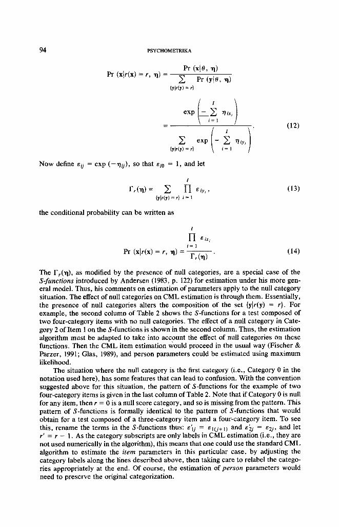
Pr (xlr(x) = r, "11) = Pr (xl O, ~1)

Pr (ytO, ,q) {y l r (y ) = r}

Z {y l r (y ) = r}

( ) _

1

exp ~ r/iyi i = 1

(12)

Now define e 0 = exp ( - ~ i j ) , so that eio = 1, and let

l

rr(~l) = ~ H ely,, {y l r (y ) = r} i = 1

(13)

the conditional probability can be written as

Pr (xlr(x)= r, 1 1 ) = - -

I

1-I ei~, i = 1

Fr(-q) (14)

The F r ( ' q ) , a s modified by the presence of null categories, are a special case of the S-functions introduced by Andersen (1983, p. 122) for estimation under his more gen- eral model. Thus, his comments on estimation of parameters apply to the null category situation. The effect of null categories on CML estimation is through them. Essentially, the presence of null categories alters the composition of the set {ylr(y) = r}. For example, the second column of Table 2 shows the S-functions for a test composed of two four-category items with no null categories. The effect of a null category in Cate- gory 2 of Item 1 on the S-functions is shown in the second column. Thus, the estimation algorithm must be adapted to take into account the effect of null categories on these functions. Then the CML item estimation v¢ould proceed in the usual way (Fischer & Parzer, 1991; Glas, 1989), and person parameters could be estimated using maximum likelihood.

The situation where the null category is the first category (i.e., Category 0 in the notation used here), has some features that can lead to confusion. With the convention suggested above for this situation, the pattern of S-functions for the example of two four-category items is given in the last column of Table 2. Note that if Category 0 is null for any item, then r = 0 is a null score category, and so is missing from the pattern. This pattern of S-functions is formally identical to the pattern of S-functions that would obtain for a test composed of a three-category item and a four-category item. To see this, rename the terms in the S-functions thus: e' t j = e l ( j + l ) and e'2j = e2 j , and let r' = r - 1. As the category subscripts are only labels in CML estimation (i.e., they are not used numerically in the algorithm), this means that one could use the standard CML algorithm to estimate the item parameters in this particular case, by adjusting the category labels along the lines described above, then taking care to relabel the catego- ries appropriately at the end. Of course, the estimation of person parameters would need to preserve the original categorization.

MARK WILSON AND GEOFFERY N. MASTERS

TABLE 2

Combinatorial Functions for a Test with Two Four-category Items

95

No Null Categories Item 1, Category 2 Null Item 1, Category 0 Null

E 10E20 = 1 E 10E20 = 1

E11E20 + EIOE21 EIIE20 + EIoE21 EIIE20 =I

E12E20 + E10E22 + EllE21 E10~22 + EllE21 E12E20 + EllE21

E13E20 + E10E23 + EI2E21 + EllE22 E13E20 + E10~23 + E12E2I E13E20 + E12E21 + EllE22

E13E21 + ~11E23 + ~121~22 E13E21 + EllE23 E13E21 + EllE23 + 1~12E22

E13E22 + EI2E23 E13E22 E13E22 + E12E23

E13E23 E13E23 E13E23

Joint Max imum Likelihood Estimation

Joint maximum likelihood (JML) estimation (also known as unconditional maxi- mum likelihood estimation) has been shown to be inconsistent (Andersen, 1973), al- though correction factors may be used to lessen the inconsistency, especially in tests with larger numbers of items (Wright & Masters, 1982). Computer programs that use the JML approach are widely available and are used in many practical applications (Wright, Congdon, & Schultz, 1988; Wright, Masters, & Ludlow, 1982). In the presence of null categories, estimation using a JML approach that can be carried out analogously to that described in Masters (1982). Consequently, Masters ' parameterization will be used in what follows.

Define a vector qi for each item i as follows: if ca tegory j is null, let qij = 0; if ca tegory j is not null, but is the lowest nonnull category b(i), let qib(i) = 0; otherwise, let qij = J - J ' , where j ' is the next nonnull category below j .

Then, for a four category item with no null categories, qi = (0, 1, 1, 1), for one with a null category for Category 2, qi = (0, 1, 0, 2), but for one with Category 0 null, qi -- (0, 0, 1, 1). Then, applying (7) to (1), the conditional probability of ca tegory j is modeled as:

Pr (xi =jlo, gi) = 0, if j < b(i), (15)

Pr (xi =j ) ]0 , ~i) = m(i) t

1 + ~ exp ~ q i k ( O - 8ik'k) t = l k = l

, i f j = b(i), (16)

and

96 PSYCHOMETRIKA

Pr (xi =j)lO, ~i) =

exp J

Z k = l

q i k ( O -- t~ik'k)

re(i) t

1+ Z exp Z t = l k = l

qik(O - ~ i k ' k )

, i f j > b(i). (17)

Note that qik for k null and k = b(i) are zero, so that although 6ik, k for k null and 6ib,( i)b(i ) formally appear in (16) and (17), they play no part, and may be left undefined.

Equations (16) and (17) are the same as those in Masters (1982) with the addition of the q6" These are multiplicative constants, so that in finding first and second deriv- atives of the log likelihood for the Newton Raphson equations, their presence has the effect of dropping some of the 6tj 7 from the equation (i.e., when qij = 0), or of inserting a constant into the equations. This introduces no major change in the estima- tion procedure, so the details will not be shown here. This JML procedure has been implemented in the computer program Quest (Adams & Khoo, 1992).

An Example

The following example uses data from a study of a new statistics curriculum for high schools (Webb, Day, & Romberg, 1988). The seven items consist of a short piece of stimulus material that might consist of text, tables, or figures, followed by open- ended questions concerning the material (Romberg, Collis, Donovan, Buchanan, & Romberg, 1982; Romberg, Jurdack, CoUis, & Buchanan, 1982). These questions are scored to correspond to levels of the SOLO taxonomy (Biggs & Collis, 1982), although in this case, because of the age of the students, the uppermost level (extended abstract) was not evaluated. For the purposes of this illustration, we will not interpret the SOLO levels themselves, but we do want to use the fact that the SOLO theory was used to generate the items as the basis for the assumption that the levels indicated by the scores for each item have a priori substantive significance. We will use a data set that has no null categories, and will artificially create several null categories. This is done not because of a shortage of examples of null categories, but because we judge that it is useful for illustrative purposes to be able to compare the results from the original data set with the results from the data set with artificial null categories.

The left-hand side of Table 3 displays the category counts for the 1237 students in the original data set. To simulate the two types of null category situations, we created an artificial data set by deleting all students who scored I on item 2, and all those who scored either 0 or 1 on item 4. The resulting category counts for the artificial data set, with null categories preserved, are shown on the right hand side of Table 3. The downcoded data set would appear the same as for the null categories data set except for Items 2 and 4. For Item 2, the counts for Categories 2 and 3 would be moved to Categories I and 2, respectively, and the count for Category 3 would be zero. For Item 4, the counts for Categories 2 and 3 would be swapped with those for 0 and I, respec- tively. The JML program Titan (Adams & Khoo, I992) was applied to the original data set, to the artificial data set, and to the downcoded version of the artificial data set.

Table 4 gives the item parameters and their standard errors for the three analyses. For items other than 2 and 4, the estimates are substantially the same. Note that one should not expect any of the results for the original and artificial data sets to be identical, as they are based on different sets of persons, but because the number of persons deleted from the original data set was relatively small, they should not be

MARK WILSON AND GEOFFERY N. MASTERS

T A B L E 3

Original Data and Artificial Data for Example Described in Text

97

Original Data Artificial Data

Item 0 1 2 3 0 1 2 3

1 43 130 344 720 32 111 305 645

2 29 67 744 397 19 0 687 387

3 39 86 1069 43 33 67 952 41

4 19 64 752 401 0 0 704 389

5 29 189 668 350 18 149 598 328

6 248 582 291 116 198 509 273 113

7 360 355 173 349 287 309 165 332

strikingly different. For Item 4, where the null categories are extremal, the downcoded analysis has given basically the same estimate as the null category analysis (taking standard errors into account). Thus, for item parameter estimation under these circum- stances, downcoding causes little problem. For Item 2, the effect of the downcoding has been quite dramatic on the 6202 parameter. Even though, as an estimate well below the floor of the person distribution, this parameter has a much larger standard error than the others, the difference between the downcoded estimate and the null category estimate is large. Interestingly, there has been relatively little effect on the estimation of the 3223

parameter. Clearly this would be a very important consideration if one were to try to interpret the item parameter estimates. The effect of downcoding on person parameter estimates can be considered by examining one or two examples. For instance, a person with the response vector (2,2,2,2,2,2,2) would score 14 in both the original and null categories data sets, giving estimates of 0.73 (s.e. = .45) and 0.85 (s.e. = .52), respec- tively, and would score 11 in the downcoded data set, giving an estimate of .40 (s.e. -- .47). As a second example, a person with the response vector (1,0,1,2,1,1,1) would score 7 in both the original and null categories data sets, giving estimates of - . 69 (s.e. = .43) and - .66 (s.c. = .45), respectively, and would score 5 in the downcoded data set, giving an estimate of - .93 (s.c. = .51). Thus, the effect of downcoding in this case has been to reduce person parameter estimates by approximately 0.3 logits, or about 0.66 of a standard error. Although this difference is not statistically significant at

98 PSYCHOMETRIKA

TABLE 4

Comparison of Item Parameters in Example

Original data Null levels Downcode

Item Categories Estimate Std. Error Estimate Std. Error Estimate Std. Error

1 0/1 -0.87 .18 -0.81 .20 -0.81 .20 1/2 -0.52 .10 -0.52 .11 -0.46 .11 2/3 -0.09 .08 -0.08 .09 -0.04 .09

2 0/2 -0.94 a .13 -1.30 .14 -2.10 .24 2/3 0.61 .09 0.76 .09 0.83 .10

3 0/1 -0.69 .19 -0.57 .20 -0.52 .20 1/2 -1.06 .12 -1.07 .13 -1.04 .13 2/3 1.95 .18 1.92 .18 1.98 .18

4 2/3 0.60 .09 0.96 .07 1.01 .07 5 0/1 -1.16 .21 -1.18 .25 -1.13 .25

1/2 -0.56 .10 -0.59 .11 -0.55 .11 2/3 0.67 .09 0.63 .09 0.69 .09

6 0/1 -0.40 .09 -0.42 .10 -0.38 .10 1/2 0.61 .09 0.57 .09 0.63 .09 2/3 1.12 .12 1.09 .13 1.13 .13

7 0/1 -0.05 .08 -0.07 .09 -0.02 .09 1/2 0.53 .08 0.48 .09 0.52 .09 2/3 0.24 .09 0.23 .09 0.28 .09

a This estimate was calculated using (7), and its standard error was calculated accordingly.

the individual level, it is a noticeable amount of bias, and would be statistically signif- icant when comparing groups of persons of a certain size.

Discussion

The strategy described above provides a straightforward way to avoid what has been a problem in the application of the PCM, especially to those following the for- mulation of Masters and Wright (Masters, 1982; Wright & Masters, 1982). The use of the extended item parameters allows for an interpretation involving the CCCs that is visually intuitive and very helpful in communicating with applications-oriented re- searchers for whom mathematical conventions, such as setting certain parameters to

MARK WILSON AND GEOFFERY N. MASTERS 99

zero has little meaning. We have not discussed the case of marginal maximum likeli- hood estimation in the presence of null categories as it assumes a particularly straight- forward character in the formulation of Wilson and Adams (in press), and is discussed there. Application of this technique to other models in the family described by Wright and Masters (1982) will follow along similar lines.

References

Adams, R. A., & Khoo, S. T. (1992). Quest [computer program]. Hawthorn, Australia: Australian Council for Educational Research.

Andersen, E. B. (1972). The numerical solution of a set of conditional estimation equations. Journal of the Royal Statistical Society, Series B, 34, 42-50.

Andersen, E. B. (1973). Conditional inference for multiple choice questionnaires. British Journal of Math- ematical and Statistical Psychology, 26, 31-44.

Andersen, E. B. (1977). Sufficient statistics and latent trait models. Psychometrika, 42, 69-81. Andersen, E. B. (1983). A general latent structure model for contingency table data. In, H. Wainer & S.

Messick (Eds.), Principals of modern psychological measurement (pp. 117-138). Hillsdale, NJ: Lawrence Erlbaum.

Biggs, J. B., & Collis, K. F. (1982). Evaluating the quality of learning: The SOLO taxonomy. New York: Academic Press.

Fienberg, S. (1977). The analysis of cross-classified categorical data. Cambridge, MA: MIT Press. Fischer, G. H. (1974). Einfiihring in die theorie psychologischer tests [Introduction to the theory of psycho-

logical tests]. Berne: Huber Verlag. Fischer, G., & Parzer, P. (1991). An extension of the rating scale model with an application to the measure-

ment of change. Psychometrika, 56, 637-652. Glas, C. A. W. (1989). Contributions to estimating and testing Rasch models. Unpublished doctoral disser-

tation, Twente University, Twente, The Netherlands. Glas, C. A. W. (1991, April). Testing Rasch models for polytomous items with an example concerning

detection of item bias. Paper presented at the annual meeting of the American Educational Association, Chicago.

Gustafsson, J. E. (1980). Testing and obtaining fit of data to the Rasch model. British Journal of Mathemat- ical and Statistical Psychology, 33, 205-233.

Jansen, P. G. W., & Roskam, E. E. (1986). Latent trait models and dichotomization of graded responses. Psychometrika, 51, 69-91.

Masters, G. N. (1982). A Rasch model for partial credit scoring. Psychometrika, 47, 149-174. Masters, G. N., & Wright, B. D. (1984). The essential process in a family of measurement models. Psy-

chometrika, 49, 529-544. Rasch, G. (1960). Probabilistic models for some intelligence and attainment tests. Copenhagen: Denmark's

Paedagogistic Institut. Romberg, T. A., CoUis, K. F., Donovan, B. F., Buchanan, A. E., & Romberg, M. N. (1982). The develop-

ment of mathematical problem solving superitems (Report of NIE/EC Item Development Project). Madison, WI: Wisconsin Center for Education Research.

Romberg, T. A., Jurdak, M. E., Collis, K. F., & Buchanan, A. E. (1982). Construct validity of a set of mathematical superitems (Report on NIE/ECS Item Development Project). Madison, WI: Wisconsin Center for Education Research.

Webb, N. L., Day, R., & Romberg, T. A. (1988). Evaluation of the use of"Exploring Data" and "'Exploring Probability". Madison, WI: Wisconsin Center for Education Research.

Wilson, M., & Adams, R. A. (in press). Marginal maximum likelihood estimation for the ordered partition model. Journal of Educational Statistics.

Wright, B., Congdon, R., & Schultz, M. (1988). MSTEPS [computer program]. Chicago: University of Chicago, MESA Psychometrics Laboratory.

Wright, B., & Masters, G. N. (1982). Rating scale analysis. Chicago: MESA Press. Wright, B., Masters, G. N., & Ludlow, L. H. (1982). CREDIT [computer program]. Chicago: MESA Press.

Manuscript received 10/22/90 Final version received 4/6/92