The Origins of Aggregate Fluctuations in a Credit Network ...

The Origins of Aggregate Fluctuations in a Credit NetworkEconomy∗

Levent Altinoglu†

October 16, 2016

Abstract

I show that inter-firm lending plays an important role in business cycle fluctuations.I first build a network model of the economy in which trade in intermediate goods isfinanced by supplier credit. In the model, a financial shock to one firm affects its abilityto make payments to its suppliers. The credit linkages between firms then transmitfinancial shocks across the economy, amplifying their effects on aggregate output. Tocalibrate the model, I construct a proxy of inter-industry credit flows from firm- andindustry-level data. Counterfactual exercises suggest these credit network effects can bea powerful amplification mechanism. I estimate aggregate and idiosyncratic shocks toindustries in the US and find that financial shocks are a prominent driver of observedcyclical fluctuations: more than two-thirds of the drop in industrial production during theGreat Recession is accounted for by financial shocks. Furthermore, idiosyncratic financialshocks to a few key industries can explain a considerable portion of these effects. Incontrast, while productivity shocks played a meaningful role before 2007, they had adecidedly negligible impact during the Great Recession.

∗I am very grateful to my advisors Stefania Garetto, Simon Gilchrist, and Adam Guren for their guidance.I also thank Giacomo Candian, Maryam Farboodi, Mirko Fillbrunn, Illenin Kondo, Fabio Schiantarelli, andparticipants of the BU macro workshop, Federal Reserve Board seminars, and BU-BC Green Line MacroMeeting, INET seminar at Columbia University, Econometric Society NASM, and EEA-ESEM for commentswhich substantially improved this paper. All errors are my own.†Columbia University. Email: [email protected]. Website: blogs.bu.edu/levent

Introduction

The recent financial crisis and ensuing recession have underscored the importance of ex-ternal finance for the real economy. Generally, firms obtain most of their short-term externalfinancing from their suppliers, in the form of delayed payment terms for their purchases. Inspite of its importance, the aggregate implications of these lending relationships remain poorlyunderstood.

In this paper, I show that inter-firm lending plays an important role in business cyclefluctuations. To this end, I introduce supplier credit into a network model of the economyand show, analytically and quantitatively, that the credit network of an economy amplifies theeffects of financial shocks. I then use my framework to empirically shed light on the originsof observed business cycle fluctuations in the US.

My approach involves three steps. First, I provide intuition with a stylized model in whichtrade in intermediate goods is financed by supplier credit. In this model, a shock to one firm’sliquid funds reduces its ability to make payments to its suppliers. The credit linkages betweenfirms and their suppliers thus propagate the firm-level shock across the network, amplifyingits aggregate effects. Second, I calibrate the model to assess the quantitative importance ofthese credit network effects. For this, I construct a proxy of the credit linkages between USindustries by combining firm-level balance sheet data and industry-level input-output data.Finally, I estimate shocks to these industries using two empirical approaches: by estimatingan identified VAR, and by performing a structural factor analysis of the model. Accountingfor the propagation mechanisms of credit and input-output interlinkages reveals the centralimportance of financial shocks as a driver of US business cycle fluctuations.

The credit linkages that I model take the form of trade credit, or delayed payment terms,that suppliers of intermediate goods often extend to their customers. Trade credit is the singlemost important source of short-term external finance for firms, and facilitates most inter-firmtrade. In the US, trade credit was three times as large as bank loans and fifteen times as largeas commercial paper outstanding on the aggregate balance sheet of non-financial corporationsin 2012.1 In most OECD countries, trade credit accounts for more than half of firms’ short-term liabilities and more than one-third of their total liabilities.2 All of these facts point tothe presence of strong credit linkages between non-financial firms.

An important feature of trade credit is that it leaves suppliers exposed to the financialdistress of their customers. Anecdotal evidence has long suggested that when firms play a dual

1During the Great Recession, the dry-up of trade credit was comparable to that of bank lending, with apeak-to-trough decline of about 25 percent. See the Federal Reserve Board’s Flow of Funds.

2A large empirical literature documents the pervasiveness of trade credit. Generally, trade credit contractsare last for as short as 15 days to as long as several months. See Petersen and Rajan (1997) for more information.

1

role of supplier and creditor, delays in payment may transmit financial distress from firmsto their suppliers.3 There is growing evidence to suggest that this intuition is empiricallyrelevant. A number of studies - including Jacobson and von Schedvin (2015), Boissay andGropp (2012), Raddatz (2010), and Kalemli-Ozcan et al. (2014) - have found that firm- andindustry-level trade credit linkages propagate financial shocks from firms to their suppliers.In spite of this evidence, the macroeconomic implications of trade credit have been largelyoverlooked in the literature. I therefore develop a framework for understanding how inter-firmtrade and credit interact in response to changing credit conditions.

I consider an economy similar to that of Bigio and La’O (2016), in which firms are or-ganized in a production network and trade intermediate goods with one another. Limitedenforcement problems require firms to make cash-in-advance payments to their suppliers be-fore production takes place. However, firms can delay part of these payments by borrowingfrom their suppliers. I assume that, to obtain this credit, a firm can credibly pledge somefraction of its future cash flow to repay its suppliers. Importantly, this implies that the cash-in-advance payments collected by each firm are endogenous to the model, and depend on theprices of its customers’ goods. As it turns out, endogenous changes in firms’ cash-in-advanceconstraints are crucial for how the economy behaves in response to shocks.

When one firm is hit with an adverse shock to its cash on hand, there are two channelsby which other firms in the economy are affected. First is the standard input-output channel,which has been the focus of studies such as Acemoglu et al. (2012) and Bigio and La’O (2016):the shocked firm cuts back on production, reducing the supply of its good to its customers.Second is a new credit linkage channel which tightens the financial constraints of upstreamfirms. That is, when the shocked firm cuts back on production, the price of its good rises.This increases the collateral value of its future cash flow, allowing the firm to reduce the cash-in-advance payments it makes to its suppliers. Being more cash-constrained, these suppliersmay be forced to cut back on their own production, and reduce the CIA payments to theirown suppliers (and so on and so forth). In this way, these credit network effects amplify thefirm-level shock in a manner which depends on the underyling structure of the credit network.

Next, I evaluate the quantitative relevance of the mechanism. In order to calibrate themodel, I first construct a proxy of inter-industry trade credit flows by combining firm-levelbalance sheet data from Compustat with industry-level input-output data from the Bureau ofEconomic Analysis. With this, I produce a map of the credit network of the US economy atthe three-digit NAICS level of detail. I calibrate the model to match this proxy and the input-output matrices of the US. I also allow for substitutability between cash and bank credit, so

3 For example, the government bailout of the US automotive industry in 2008 was precipitated by an acuteshortage of liquidity, which came about largely due to extended delays in payment for goods already delivered.

2

that firms can partially offset a loss in customer payments with increased bank borrowing.Counterfactual exercises reveal that the propagation mechanism is quantitatively signifi-

cant - in response to an aggregate financial shock, the credit network of the US amplifies the fallin GDP by 28 percent. Furthermore, the aggregate impact of an idiosyncratic (industry-level)financial shock depends jointly on the underlying structures of the credit and input-outputnetworks of the economy. Based on this analysis, certain industries emerge as systemicallyimportant to the US economy.

In the empirical part of the paper, I use this theoretical framework to investigate whichshocks drive cyclical fluctuations once we account for the network effects created by creditinterlinkages. My framework is rich enough to permit an empirical exploration of the sourcesof these fluctuations along two separate dimensions: the importance of productivity versusfinancial shocks, and that of aggregate versus idiosyncratic shocks. To address these issues, Iuse two methodological approaches.

My first approach involves identifying financial and productivity shocks without imposingthe structure of my model on the data. To do this, I first construct quarterly measures ofbank lending based on data from Call Reports collected by the FFIEC. I then augment anidentified VAR of macro and monetary variables with this measure of bank lending, and withthe excess bond premium (EBP) of Gilchrist and Zakrajsek (2012), which reflects the risk-bearing capacity of the financial sector. I then construct financial shocks as changes in banklending which arise from orthogonalized innovations to the EBP. 4 For productivity shocks, Iuse the quarterly, utilization-adjusted changes in TFP estimated by Fernald (2012).

Feeding these estimated shocks into the model, I find that, before 2007, productivityand financial shocks played a roughly equal role in generating cyclical fluctuations, togetheraccounting for half of observed aggregate volatility in US industrial production (IP). However,during the Great Recession, productivity shocks had virtually no adverse effects on IP - infact, they actually mitigated the downturn. On the other hand, two-thirds of the peak-to-trough drop in aggregate IP during the recession can be accounted for by financial shocks,with the remainder unaccounted for by either shock. In addition, the credit network of theseindustries played a quantitatively important role in exacerbating the effects of financial shocks,accounting for nearly a fifth of the fall in IP.

With my second methodological approach, I empirically assess the relative contributionof aggregate versus idiosyncratic shocks in generating cyclical fluctuations. This involvesestimating the model using a structural factor approach similar to that of Foerster, Sarte,and Watson (2011), using data on the output and employment growth of US IP industries. I

4 I construct the measure of bank lending in such a way that changes in the demand for bank lending arelargely netted out. Therefore, changes in my measure of bank lending mostly reflect supply-side changes.

3

first use a log-linear approximation of the model to back-out the productivity and financialshocks to each industry required for the model to match the fluctuations in the output andemployment data. Then, I use standard factor methods to decompose each of these shocksinto an aggregate component and an idiosyncratic component.

Through variance decomposition I show that, while the idiosyncratic component of pro-ductivity shocks can explain a substantial fraction of aggregate volatility before 2007, it playedvirtually no role during the Great Recession. Rather, nearly three-quarters of the drop in IPduring the recession can be accounted for by aggregate financial shocks. In addition, theremainder can be accounted for by idiosyncratic financial shocks to a few systemically im-portant IP industries - namely the oil and coal, chemical, and auto manufacturing industries.Furthermore, the credit and input-output linkages between industries played a significant rolein propagating these industry-level shocks across the economy.

The broad picture which emerges from these two empirical analyses is that financial shockshave been a key driver of aggregate output dynamics in the US, particularly during the GreatRecession. While shocks to aggregate TFP have long been relied upon as a principal sourceof cyclical fluctuations, the lack of direct evidence for such shocks has raised questions abouttheir empirical viability. On the other hand, the credit and input-output interlinkages offirms can create a powerful mechanism by which a shock to one firm’s financial constraintpropagates across the economy. When we account for this amplification mechanism, financialshocks seem to displace aggregate productivity shocks as a prominent driver of the US businesscycle.

Related Literature

This paper contributes to several strands of the literature. A growing literature examinesthe importance of network effects in macroeconomics, including Acemoglu et al. (2012),Shea (2002), Dupor (1999), Horvath (2000), Acemoglu et al. (2015), Baqaee (2016), andCarvalho and Gabaix (2013). These abstract away from financial frictions. The notablework of Bigio and La’O (2016), explore the interaction between financial frictions and theinput-output structure of an economy. However, they do not explicitly model any creditrelationships between firms. Luo (2016) embeds an input-output structure in the frameworkof Gertler and Karadi (2011), with a role for trade credit. However, trade credit linkagesdo not propagate shocks across the economy per se.5 Kiyotaki and Moore (1997) studytheoretically how a shock to a firm in a credit chain can cause a cascade of defaults in a partialequilibrium framework. Gabaix (2011), Foerster et al. (2011), and Stella (2014) evaluate thecontribution of idiosyncratic shocks to aggregate fluctuations, the latter two using a structural

5 Credit linkages only affect the interest rate that the bank charges firms. As such, all network effects aredue to input-output linkages, as in Bigio and La’O (2016).

4

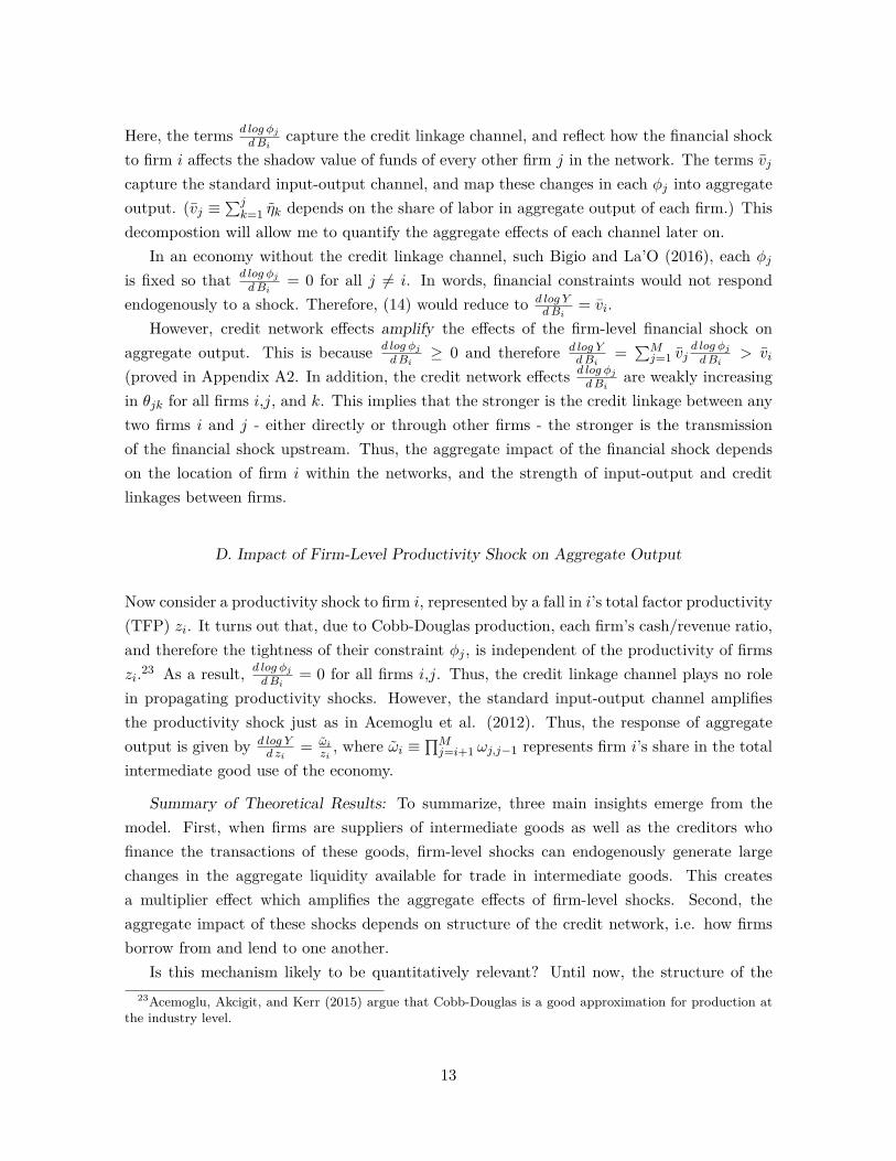
Figure 1: Vertical Production Chain

factor approach. Jermann and Quadrini (2012) evaluate the importance of financial shocksby explicitly modelling the tradeoff between debt and equity financing.

The rest of the paper is organized as follows. In section I, I introduce the stylized model andderive the analytical results. In sections II-IV, I generalize the production network structure,discuss the construction of my proxy for credit flows and calibration, and summarize thequantitative results. In section V, I perform the empirical analyses.

I. Stylized Model: Vertical Production Structure

In this section, I build intuition with a simple model. The stylized nature of the productionstructure of the economy permits closed-form expressions for equilibrium variables. I willlater generalize both the production structure and preferences.

There is one time period, consisting of two parts. At the beginning of the period, contractsare signed. At the end of the period, production takes place and contracts are settled. Thereare three types of agents: a representative household, firms, and a bank. There are Mgoods, each produced by a continuum of competitive firms with constant returns-to-scale inproduction. We can therefore consider each good as being produced by a representative,price-taking firm. Each good can be consumed by the household or used in the production ofother goods.

The representative household supplies labor competitively to firms and consumes a finalconsumption good. . It has preferences over consumption C and labor N given by U(C,N),and a standard budget constraint, where w denotes the competitive wage earned from working,and πi the profit earned by firm i.

U(C,N) = log C −N C = wN +M∑i=1

πi (1)

There are M price-taking firms who each produce a different good, for now arranged ina supply chain, where each firm produces an intermediate good for one other firm. The lastfirm in the chain produces the consumption good, which it sells to the household. Firms areindexed by their order in the supply chain, with i = M denoting the producer of the finalgood.

The production technology of firm i is Cobb-Douglas over labor and intermediate goods,where xi denotes firm i’s output, ni its labor use, and xi−1 its use of good i − 1, zi denotes

5

firm i’s total factor productivity, ηi the share of labor in its production (and η1 = 1), andωi,i−1 the share of good i− 1 in firm i’s total intermdiate good use (equal to 1 for now). Letps denote the price of good s.

xi = zinηii x

ωi,i−1(1−ηi)i−1 (2)

Limited enforcement problems between firms create a need for ex ante liquidity to financeworking capital. The household cannot force any debt repayment. Therefore, firm i must paythe full value of wage bill, wni, up front to the household before production takes place. Inaddition, each firm i must pay for its intermediate goods purchases, pi−1xi−1 up front to itssupplier. Thus, firms are required to have some funds at the beginning of the period beforeany revenue is realized.

Firm i can delay payment to its supplier by borrowing some amount τi−1 from its supplier,representing the trade credit loan given from i − 1 to i. In addition, each firm can obtain acash loan bi from the bank. The net payment that firm i − 1 receives from its customer atthe beginning of the period is therefore pi−1xi−1 − τi−1. Firm i’s cash-in-advance constrainttakes the form

wni︸︷︷︸wage bill

+ pi−1xi−1 − τi−1︸ ︷︷ ︸CIA payment to supplier

≤ bi︸︷︷︸bank loan

+ pixi − τi︸ ︷︷ ︸CIA from customer

(3)

Thus, the cash that firm i is required to have in order to employ ni units of labor and purchasexi−1 units of intermediate good i−1, is bounded by the amount of cash that firm i can collectat the beginning of the period. Note that trade credit appears on both sides of the constraint.

Firms face borrowing constraints on the size of loans they can obtain from their suppliersand the bank. Firm i can obtain the loan bi from the bank at the beginning of the periodby pledging a fraction Bi of its total end-of-the-period revenue pixi, and a fraction α of itsaccounts receivable τi+1, where α ε (0, 1].6

bi ≤ Bipixi + ατi (4)

Firms are also constrained in their ability to obtain trade credit from their suppliers. Inparticular, firm i can credibly pledge a fraction θi of its end-of-the-period revenue to repayits supplier.

τi−1 ≤ θipixi (5)6 I will later show that α parameterizes the degree of substitutability between cash and bank credit.

6

How do firms choose how much to lend to their customers and borrow from their suppliers?Recall that representative firm i is actually comprised of a continuum of competitive firmswith CRS production. Perfect competition amongst these suppliers forces them to offer theircustomers the maximum amount of trade credit permitted by the constraint. This resultholds even when these suppliers are cash-constrained in equilibrium.7 (I leave the proof ofthis to an online appendix.) While this pins down the supply of trade credit, I study firms’demand for trade credit below.

We can re-write firm i’s cash-in-advance constraint as

wni + pi−1xi−1 ≤ χipixi︸ ︷︷ ︸liquid funds

(6)

where

χi ≡bipixi

+ τi−1pixi︸ ︷︷ ︸

debt/revenue ratio

+ 1− τipixi︸ ︷︷ ︸

cash/revenue ratio

(7)

Therefore, a firm’s expenditure on inputs is bounded by the amount of funds it has at thebeginning of the period. The variable χi describes the tightness of firm i’s cash-in-advanceconstraint, and will play a key role in the mechanism of the model. The tightness of a firm’scash-in-advance constraint is comprised of the firm’s debt-to-revenue ratio and its cash-to-revenue. These describe how much of the firm’s revenue is financed by debt, and how much ofits revenue is collected as a cash-in-advance payment, respectively. Notice that χi is decreasingin τi

pixi, the amount of i’s output sold on credit: the more credit that i gives its customer, the

less cash it collects at the beginning of the period.Firm i chooses its input purchases ni and xi−1, and how much trade credit to borrow

τi−1, to maximize its profits subject to its cash-in-advance constraint. (Recall that becauseof perfect competition, the firm takes its trade credit lending τi as given.)

maxni, xi−1, τi−1

pixi − wni − pi−1xi−1

s.t. wni + pixi−1 ≤ χi(τi−1)pixi (8)

τi−1 ≤ θipixi (9)

Denote by τ∗i−1 firm i’s choice of how much trade credit to borrow from its supplier. I show inonline appendix O.A1 that if firm i’s cash-in-advance constraint (8) is binding in equilibrium,then it borrows the maximum amount of trade credit offered by its supplier, pinning downτ∗i−1 = θipixi. For much of this paper, I consider this more interesting case in which firms are

7These results are supported by micro-level evidence on trade credit: competition amongst suppliers is isoften sufficiently high that they are forced to offer their customers extended payment terms, even when theyare cash-constrained. See, for instance, Barrot (2015).

7

constrained in equilibrium.8

If firms are constrained in equilibrium, we can re-write the tightness χi of a firm’s con-straint using firms’ binding borrowing constraints to replace τi and bi.

χi = Bi + θi︸ ︷︷ ︸debt/revenue ratio

+ 1− (1− α)θi+1pi+1xi+1pixi︸ ︷︷ ︸

cash/revenue ratio

(10)

Crucially, equation (4) shows that χi is an equilibrium object - it is an endogenous variablewhich depends on the firm’s forward credit linkage θi+1 and the revenue of its customer.9

Hence, changes in the price of its customer’s good affect the tightness of firm i’s cash-in-advance constraint. 10 Here, the endogeneity of χi will be a critical determinant of how theeconomy responds to shocks.

Firm i’s optimality conditions equate the ratio of expenditure on each type of input withthe ratio of their share of production. I show in Appendix A3 that firm i’s cash-in-advanceconstraint (3) binds in equilibrium if and only if χi < 1. Combining the first order conditionswith the cash-in-advance constraint yields the optimality conditions below.11

w = φiηipixini

, pi−1 = φiωi,i−1(1− ηi)pixixi−1

(11)

Here, φi ≡ min 1, χi describes firm i’s shadow value of funds.12 φi is strictly less than oneif and only if firm i’s cash-in-advance is binding in equilibrium. Equations (5) says that, ifbinding, the cash-in-advance constraint inserts a wedge φi < 1 between the marginal cost andmarginal benefit of each input, representing the distortion in the firm’s input use created bythe constraint. A tighter cash-in-advance (lower χi) corresponds to a greater distortion, andlower output. Through χi , φi endogneously depends on shadow value funds of downstreamfirms φi+1, reflecting that firms’ constraints are interdependent due to trade credit.

Note that there are two types of interlinkages between firms: input-output linkages, repre-sented by input shares ωi,i−1 in production; and credit linkages, represented by the borrowinglimits θi between firms. Each of these interklinkages will play a different role in generatingnetwork effects from shocks.

8Nevertheless that (9) binds in equilibrium is not crucial for the qualitative results, and may in fact under-state the quantitative results.

9 Notice that the firm’s debt-to-revenue ratio is fixed, because firms collateralize their end-of-period revenuefor borrowing.

10This a key difference with Bigio and La’O (2016), in which the tightness of each firm’s cash-in-advance isan exogenous parameter because there is no inter-firm lending.

11Since τi−1 is important only insofar as it affects the tightnesses of firms’ constraints, it shows up in firmi’s first order conditions only through φi.

12More precisely, the shadow value of funds of firm i is given by 1φi− 1.

8

A. Equilibrium

I close the model by imposing labor and goods market clearing conditions N =∑Mi=1 ni

and C = Y ≡ xM .

Definition: An equilibrium is a set of prices piiεI , w , and quantities xi, ni, τiiεI that (i)maximize the representative household’s utility, subject to its budget constraint; (ii) maximizeeach firm’s profits subject to its cash-in-advance, bank borrowing, and supplier borrowingconstraints; and (iii) clear goods markets and the labor market.

Equilibrium aggregate output in the economy is determined by each firm’s productionfunction and financial constraint. To see this, let Y denote the aggregate output that wouldprevail in a frictionless input-output economy (à la Acemoglu et al. (2012)), given by Y ≡∏Mi=1 η

ηii z

ωii .13 Define aggregate liquidity in the economy as Φ ≡

∏Mi=1 φ

∑i

j=1 ηj

i , an aggregationof all firm’s shadow value of funds. Then an analytical expression for equilibrium aggregateoutput, derived in Appendix A5, shows output to be log-linear in Y and the aggregate liquidityin the economy.

Y = Y Φ (12)

Intuitively, (12) says that equilibrium aggregate output is constrained by aggregate liquid-ity - the funds available to all firms to finance working capital at the beginning of the period.Note that if all firms are unconstrained, then Φ = 1 and Y = Y . If one firm i is constrained,aggregate output depends on how its constraint affects the supply of intermediate good i forall downsream firms, given by

∑ij=1 ηj .14

To summarize, firms’ financial constraints distort production in a way which depends onthe credit and input-output structures of the economy. The tightness of each firm’s constraintin turn depends on trade credit, and is therefore determined by the underlying structure ofthe credit network of the economy. At this stage, it is worth discussing how this economycompares to that of Bigio and La’O (2016). A novelty of Bigio and La’O (2016) is to show howfirm-level financial constraints affect aggregate output through the input-output structure ofthe economy. However, because all payments between firms are settled at the end of theperiod after production takes place, there is no role for trade credit in Bigio and La’O (2016),and so financial constraints φi are fixed exogenously. As I show in the next section, when

13Here, ωi ≡∏M

j=i+1 ωj,j−1 denotes firm i’s share in total intermediate good use, and ηi ≡ ηiωi denotes firmi’s share of labor in aggregate output.

14Note that the credit network of the economy - i.e. the set θi∀iεI - shows up implicitly in (12) througheach φi.

9

these constraints are determined endogenously by trade credit relationships, the economy canbehave qualitatively very differently in response to shocks.

B. Aggregate Impact of Firm-Level Shocks

I now examine how the economy responds to firm-level financial shocks and productivityshocks. I model a financial shock to firm i by a change in Bi, the fraction of firm i’s revenuethat the bank will accept as collateral for the bank loan. This is a reduced-form way to capturea reduction in the supply of bank credit to firm i, and represents an exogenous tightening infirm i’s financial constraint.15

If firm i is unconstrained in equilibrium, a marginal financial shock d Bi has no effect onits production - the firm has deep pockets and can absorb the shock. However, if the firm isconstrained, then it is forced to reduce production as it can no longer finance as many inputswith up front payments. In addition to this direct effect, there are two types of network effectsby which the shock affects other firms in the economy: input-output channel and the creditlinkage channel.

Network Effects: Standard Input-Output Channel: Through the first channel, which I callthe standard input-output channel, the shock propagates through input-output interlinkages,increasing firms’ input costs. This is the standard channel analyzed in in the input-outputliterature, including Acemoglu et al. (2012) and Bigio and La’O (2016). The reduction infirm i’s output increases the price pi of good i. This acts as a supply shock to the customerdownstream (firm i + 1), who is now faced with a higher unit cost of its intermediate good.In response, firm i + 1 cuts back on production, which causes the pi+1 to increase, etc.Thus, as a result of the shock to firm i, all firms downstream experience a supply shock totheir intermediate goods, and cut back on production. This amplifies the shock because asfirms reduce production, they cut back on employment which, in turn, reduces the wage andhousehold consumption.16 In addition, the shock travels upstream as suppliers adjust theiroutput to respond to the fall in demand for their intermediate goods.

Network Effects: Credit Linkage Channel: There is also a is a new, additional channelof transmission - which I call the credit linkage channel - which describes how the financial

15In the general network model in the following section, each firm sells some portion of its output directlyto the household. In this setting, one could alternatively interpret the fall in Bi as a failed payment by finalconsumer. In either case, these are idiosyncratic shocks to the firm’s liquid funds such that d χi

dBi> 0, and are

not well-represented by a change in its productivity or technology.16 This channel is ultimately driven by the input specificity in each firm’s production technology, as each

downstream firm is unable to offset the supply shock by substituting away from using good i in their production,and each upstream firm is unable to offset the demand shock by finding other customers for its good.

10

constraints of upstream firms are tightened endogenously in response to the shock.Recall that when firm i cuts back on production, the price pi of its good rises. This

increases the collateral value of its future cash flow, allowing it to delay payment for a largerfraction of its purchase from supplier i− 1.17 As a result, supplier i− 1’s cash/revenue ratiofalls, meaning the fraction of its revenue collected as up front payment falls. This tightens itscash-in-advance constraint - i.e. χi−1 falls.1819

χi−1 ↓ ≡ Bi−1 + θi−1︸ ︷︷ ︸debt/revenue ratio

+ 1− τi−1pi−1xi−1︸ ︷︷ ︸

cash/revenue ratio ↓

(13)

Thus, with less cash on-hand, the supplier i − 1 is now faced with a tighter financialconstraint itself. The supplier may therefore be forced to reduce production further, andthereby pass the shock to its own suppliers and customers. (This continues up the chain offirms). In this manner, the initial effect of the shock is amplified as upstream firms experiencetighter financial conditions.

But why doesn’t firm i − 1 reduce the trade credit it extends to i in order to increaseits cash holdings and relax its own financial constraint? Recall that representative firm i− 1actually consists of a continuum of perfectly competitive firms, and that competition amongstthese firms forces them to offer their customers the maximum trade credit loan allowed bythe borrowing constraint, even when they are themselves cash-constrained in equilibrium. 20

As a result, they are unable to reduce trade credit loans to increase their cash holdings. Thismechanism is in line with strong empirical evidence that firms in financial distress reduce theup-front payments they make to their suppliers, thereby transmitting the financial distress totheir suppliers.21

Note the role that α plays in mitigating the transmission of the shock via the creditlinkage channel. The higher that α is, i.e. the more that firm i− 1 can collateralize its tradecredit τi−1, the less that χi−1 falls in response to the shock to i. Although i − 1 receives asmaller cash-in-advance payment from its customer, it can collateralize a higher fraction ofits trade credit to obtain more credit from the bank. This reduces the loss in liquidity that it

17This is true even though the volume of trade credit τi−1 may actually fall in response to the shock.18Recall that firms’ debt/revenue ratios are fixed in equilibrium.19 More precisely, there are three effects on χi−1, the tightness of i− 1’s constraint, all of which imply that

χi−1 falls unambiguously in response to the shock d Bi. Recall from (10) that firm i− 1’s cash/revenue ratiodepends inversely on pixi

pi−1xi−1. First, the shock increases pi, as discussed above. Second, the fall in firm i’s

output increases the ratio xixi−1

due to the decreasing returns to xi−1 (since (1− ηi) < 1). And third, the fallin i’s demand reduces the price pi−1 of good i− 1. Each of these effects reduces χi−1.

20For instance, Barrot (2014) shows that competition amongst suppliers may force even cash-constrainedfirms to offer trade credit to their customers.

21See Jacobson and von Schedvin (2015), Raddatz (2010), and Boissay and Gropp (2012).

11

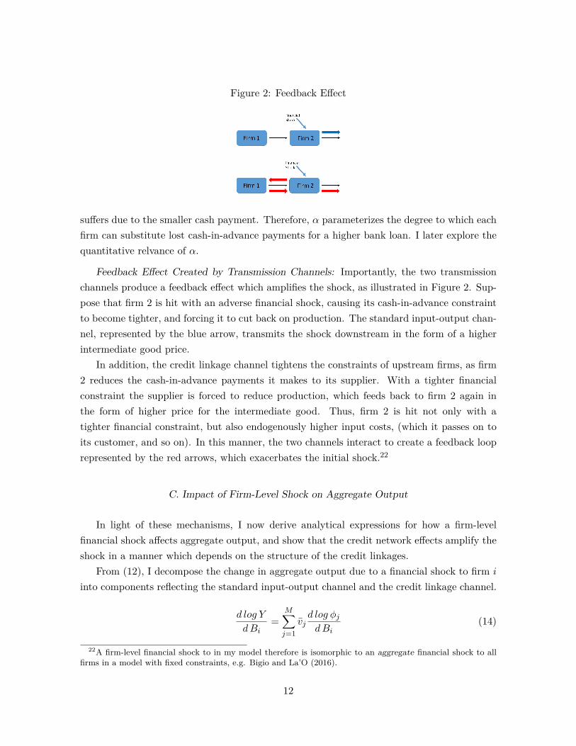
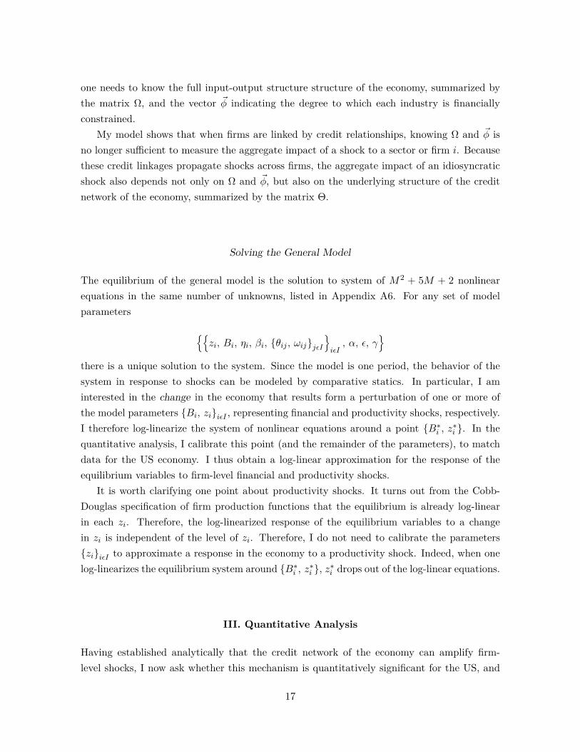
Figure 2: Feedback Effect

suffers due to the smaller cash payment. Therefore, α parameterizes the degree to which eachfirm can substitute lost cash-in-advance payments for a higher bank loan. I later explore thequantitative relvance of α.

Feedback Effect Created by Transmission Channels: Importantly, the two transmissionchannels produce a feedback effect which amplifies the shock, as illustrated in Figure 2. Sup-pose that firm 2 is hit with an adverse financial shock, causing its cash-in-advance constraintto become tighter, and forcing it to cut back on production. The standard input-output chan-nel, represented by the blue arrow, transmits the shock downstream in the form of a higherintermediate good price.

In addition, the credit linkage channel tightens the constraints of upstream firms, as firm2 reduces the cash-in-advance payments it makes to its supplier. With a tighter financialconstraint the supplier is forced to reduce production, which feeds back to firm 2 again inthe form of higher price for the intermediate good. Thus, firm 2 is hit not only with atighter financial constraint, but also endogenously higher input costs, (which it passes on toits customer, and so on). In this manner, the two channels interact to create a feedback looprepresented by the red arrows, which exacerbates the initial shock.22

C. Impact of Firm-Level Shock on Aggregate Output

In light of these mechanisms, I now derive analytical expressions for how a firm-levelfinancial shock affects aggregate output, and show that the credit network effects amplify theshock in a manner which depends on the structure of the credit linkages.

From (12), I decompose the change in aggregate output due to a financial shock to firm i

into components reflecting the standard input-output channel and the credit linkage channel.

d log Y

dBi=

M∑j=1

vjd log φjdBi

(14)

22A firm-level financial shock to in my model therefore is isomorphic to an aggregate financial shock to allfirms in a model with fixed constraints, e.g. Bigio and La’O (2016).

12

Here, the terms d log φjdBi

capture the credit linkage channel, and reflect how the financial shockto firm i affects the shadow value of funds of every other firm j in the network. The terms vjcapture the standard input-output channel, and map these changes in each φj into aggregateoutput. (vj ≡

∑jk=1 ηk depends on the share of labor in aggregate output of each firm.) This

decompostion will allow me to quantify the aggregate effects of each channel later on.In an economy without the credit linkage channel, such Bigio and La’O (2016), each φj

is fixed so that d log φjdBi

= 0 for all j 6= i. In words, financial constraints would not respondendogenously to a shock. Therefore, (14) would reduce to d log Y

dBi= vi.

However, credit network effects amplify the effects of the firm-level financial shock onaggregate output. This is because d log φj

dBi≥ 0 and therefore d log Y

dBi=∑Mj=1 vj

d log φjdBi

> vi

(proved in Appendix A2. In addition, the credit network effects d log φjdBi

are weakly increasingin θjk for all firms i,j, and k. This implies that the stronger is the credit linkage between anytwo firms i and j - either directly or through other firms - the stronger is the transmissionof the financial shock upstream. Thus, the aggregate impact of the financial shock dependson the location of firm i within the networks, and the strength of input-output and creditlinkages between firms.

D. Impact of Firm-Level Productivity Shock on Aggregate Output

Now consider a productivity shock to firm i, represented by a fall in i’s total factor productivity(TFP) zi. It turns out that, due to Cobb-Douglas production, each firm’s cash/revenue ratio,and therefore the tightness of their constraint φj , is independent of the productivity of firmszi.23 As a result, d log φjdBi

= 0 for all firms i,j. Thus, the credit linkage channel plays no rolein propagating productivity shocks. However, the standard input-output channel amplifiesthe productivity shock just as in Acemoglu et al. (2012). Thus, the response of aggregateoutput is given by d log Y

d zi= ωi

zi, where ωi ≡

∏Mj=i+1 ωj,j−1 represents firm i’s share in the total

intermediate good use of the economy.

Summary of Theoretical Results: To summarize, three main insights emerge from themodel. First, when firms are suppliers of intermediate goods as well as the creditors whofinance the transactions of these goods, firm-level shocks can endogenously generate largechanges in the aggregate liquidity available for trade in intermediate goods. This createsa multiplier effect which amplifies the aggregate effects of firm-level shocks. Second, theaggregate impact of these shocks depends on structure of the credit network, i.e. how firmsborrow from and lend to one another.

Is this mechanism likely to be quantitatively relevant? Until now, the structure of the23Acemoglu, Akcigit, and Kerr (2015) argue that Cobb-Douglas is a good approximation for production at

the industry level.

13

networks was assumed to be a straight line. So to answer this question and take the modelto the data, I now generalize certain features of the model.

II. General Model

To capture more features of the economy, I now allow for an arbitrary network structure sothat each firm may trade with and borrow from or lend to any other firm in the economy.

I assume that each of the M goods can be consumed by the representative household orused in the production of other goods. The household’s total consumption C is Cobb-Douglasover the M goods, and it has GHH preferences.24

U(C, N) = 11− γ

(C − 1

1 + εN1+ε

)1−γ, C ≡

M∏i=1

cβii (15)

Here, ε and γ respectively denote the Frisch and income elasticity of labor supply. Thehousehold maximizes its utility subject to its budget constraint (1). This yields optimalityconditions which equate the ratio of expenditure on each good with the ratio of their marginalutilities, and the competitive wage with the marginal rate of substitution between aggregateconsumption and labor.

picipjcj

= βiβj

, N1+ε = C (16)

Each firm can trade with all other firms. Firm i’s production function is again Cobb-Douglas over labor and intermediate goods.

xi = zηii nηii

m∏j=1

xωijij

1−ηi

(17)

Here, xi denotes firm i’s output and xij denotes firm i’s use of good j. Since ωij denotes theshare of j in i’s total intermediate good use, I assume

∑Mj=1 ωij = 1 so that each firm has

constant returns to scale. The input-output structure of the economy can be summarized bythe matrix Ω of intermediate good shares ωij .25

24 Quantitatively similar results hold for preferences which are additively separable in aggregate consumptionC and labor N .

25This is simply a generalization of the input-output structure in the stylized model. In that case, the Ωwould be given by a matrix of zeros, with one sub-diagonal of ones, reflecting the vertical production structureand the constant returns to scale technology of firms.

14

Ω ≡

ω11 ω12 · · · ω1M

ω21 ω22... . . .

ωM1 ωMM

Note that the production network is defined only by technology parameters. As we willsee, the presence of financial frictions will distort inter-firm trade in equilibrium. Hence, Ωdescribes how firms would trade with each other in the absence of frictions.

Each firm’s cash-in-advance constraint takes the same form as in the stylized model, withthe exception that each firm has M suppliers and M customers instead of just one of each.τis denotes the trade credit loan that firm i receives from each of its suppliers s.

wni +M∑s=1

(psxis − τis)︸ ︷︷ ︸net CIA payment to suppliers

≤ bi + pixi −M∑c=1

τci︸ ︷︷ ︸net CIA received from customers

(18)

Firm i faces borrowing constraints with each of its suppliers, to which it can pledge fractionsθis of its future cash flow to repay the loans. Each firm can also borrow bi from the bank bypledging Bi of its revenue and α of its accounts receivable

∑Mc=1 τci.

τis ≤ θispixi bi ≤ Bipixi + αM∑c=1

τci (19)

As before, competition amongst suppliers in industry s forces them to offer the maximumtrade credit permitted by the limted enforcement problem, so that the trade credit borrowingconstraint always binds when industries are cash-constrained in equilibrium. The structureof the credit network between firms can be summarized by the matrix of θij ’s.

Θ ≡

θ11 θ12 · · · θ1M

θ21 θ22... . . .

θM1 θMM

Plugging the binding borrowing constraints into (18) yields a constraint on i’s total input

purchases, where χi describes the tightness of i’s cash-in-advance constraint.

wni +M∑s=1

psxis ≤ χipixi (20)

Just as in the stylized verision, χi is an an equilibrium object, where firm i’s cash/revenueratio depends on the prices pc of its customer’s goods and its forward credit linkages θci.

15

χi = Bi +M∑s=1

θis︸ ︷︷ ︸debt/revenue ratio

+ 1− (1− α)M∑c=1

θcipcxcpixi︸ ︷︷ ︸

cash/revenue ratio

(21)

Firms choose labor and intermediate goods to maximize profits subject to their cash-in-advance constraint. Again, firm i’s contraint inserts a wedge φi between the marginal costand marginal revenue product of each input

ni = φiηipiwxi xij = φi (1− ηi)ωij

pipjxi (22)

where the wedge φi = min 1 , χi is determined by the firm’s shadow value of funds. Marketclearing conditions for labor and each intermediate good are given by

N =M∑i=1

ni xi = ci +M∑c=1

xci (23)

The equilibrium conditions of this generalized model take the same form as in the stylizedmodel, and the economy will behave in qualitatively the same way in response to shocks asin the stylized model.

For the remainder of the paper, I consider the case in which all industries are constrainedin equilibrium.26 This is to ensure that a marginal financial shock to each industry has anon-zero effect.27

Relationship Between Firm Influence and Size

A well-known critique of frictionless input-output models such as Acemoglu et al. (2012) isthat the size of a firm, as measured by its share si of aggregate sales, is sufficient to determinethe aggregate impact of a shock to sector i, and one does not need to know anything about theunderlying input-output structure of the economy. All relevant information about the input-output structure is captured by si. As a result, an idiosyncratic shock to firm i is isomporphicto an aggregate TFP shock weighted by si. This makes it impossible to distinguish the roleof idiosyncatic versus aggregate shocks in generating aggregate fluctuaions, as the two areobservationally equivalent.

Bigio and La’O (2016), however, show that this isomorphism breaks down when the econ-omy has financial frictions. To determine the aggregate impact of an idiosyncratic shock,

26The parameters Bi are set as free parameters to ensure that the calibration is consistent with this case ofthe equilibrium. This is discussed in the calibration section.

27If there are at least some firms in an industry who are constrained, then a credit supply shock will havereal effects. Therefore, assuming an industry is unconstrained will bias the results.

16

one needs to know the full input-output structure structure of the economy, summarized bythe matrix Ω, and the vector ~φ indicating the degree to which each industry is financiallyconstrained.

My model shows that when firms are linked by credit relationships, knowing Ω and ~φ isno longer sufficient to measure the aggregate impact of a shock to a sector or firm i. Becausethese credit linkages propagate shocks across firms, the aggregate impact of an idiosyncraticshock also depends not only on Ω and ~φ, but also on the underlying structure of the creditnetwork of the economy, summarized by the matrix Θ.

Solving the General Model

The equilibrium of the general model is the solution to system of M2 + 5M + 2 nonlinearequations in the same number of unknowns, listed in Appendix A6. For any set of modelparameters

zi, Bi, ηi, βi, θij , ωijjεI

iεI, α, ε, γ

there is a unique solution to the system. Since the model is one period, the behavior of thesystem in response to shocks can be modeled by comparative statics. In particular, I aminterested in the change in the economy that results form a perturbation of one or more ofthe model parameters Bi, ziiεI , representing financial and productivity shocks, respectively.I therefore log-linearize the system of nonlinear equations around a point B∗i , z∗i . In thequantitative analysis, I calibrate this point (and the remainder of the parameters), to matchdata for the US economy. I thus obtain a log-linear approximation for the response of theequilibrium variables to firm-level financial and productivity shocks.

It is worth clarifying one point about productivity shocks. It turns out from the Cobb-Douglas specification of firm production functions that the equilibrium is already log-linearin each zi. Therefore, the log-linearized response of the equilibrium variables to a changein zi is independent of the level of zi. Therefore, I do not need to calibrate the parametersziiεI to approximate a response in the economy to a productivity shock. Indeed, when onelog-linearizes the equilibrium system around B∗i , z∗i , z∗i drops out of the log-linear equations.

III. Quantitative Analysis

Having established analytically that the credit network of the economy can amplify firm-level shocks, I now ask whether this mechanism is quantitatively significant for the US, and

17

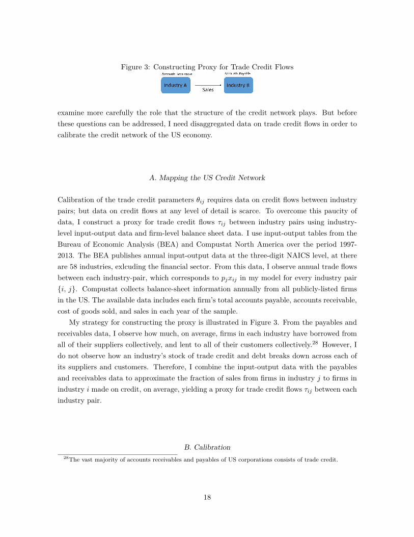
Figure 3: Constructing Proxy for Trade Credit Flows

examine more carefully the role that the structure of the credit network plays. But beforethese questions can be addressed, I need disaggregated data on trade credit flows in order tocalibrate the credit network of the US economy.

A. Mapping the US Credit Network

Calibration of the trade credit parameters θij requires data on credit flows between industrypairs; but data on credit flows at any level of detail is scarce. To overcome this paucity ofdata, I construct a proxy for trade credit flows τij between industry pairs using industry-level input-output data and firm-level balance sheet data. I use input-output tables from theBureau of Economic Analysis (BEA) and Compustat North America over the period 1997-2013. The BEA publishes annual input-output data at the three-digit NAICS level, at thereare 58 industries, exlcuding the financial sector. From this data, I observe annual trade flowsbetween each industry-pair, which corresponds to pjxij in my model for every industry pairi, j. Compustat collects balance-sheet information annually from all publicly-listed firmsin the US. The available data includes each firm’s total accounts payable, accounts receivable,cost of goods sold, and sales in each year of the sample.

My strategy for constructing the proxy is illustrated in Figure 3. From the payables andreceivables data, I observe how much, on average, firms in each industry have borrowed fromall of their suppliers collectively, and lent to all of their customers collectively.28 However, Ido not observe how an industry’s stock of trade credit and debt breaks down across each ofits suppliers and customers. Therefore, I combine the input-output data with the payablesand receivables data to approximate the fraction of sales from firms in industry j to firms inindustry i made on credit, on average, yielding a proxy for trade credit flows τij between eachindustry pair.

B. Calibration28The vast majority of accounts receivables and payables of US corporations consists of trade credit.

18

With the proxy for trade credit flows at hand, I calibrate the general model to match USdata. I calibrate technology parameters ηi and ωij to match the BEA input-output tables ofthe median year in my sample, 2005. From firm i’s optimality conditions (10), we can writethe firm’s total expenditure on inputs as

wni +M∑j=1

pjxij =

ηi + [1− ηi]M∑j=1

ωij

φipixi= φipixi

where the second equality holds due to the constant returns to scale of i’s production tech-nology. This implies that

φi =wni +

∑Mj=1 pjxij

pixi(24)

The right-hand side of (12) is directly observable from the BEA’s Direct Requirements table.Looking through the lense of the model, the observed input-output tables reflect both

technology parameters and distortions created by the liquidity onstraints. My calibrationstrategy respects this feature. In particular, I calibrate technology parameters using firm i’soptimality conditions for each input and my calibrated φi’s

ηi = wniφipixi

ωij = pjxij(1− ηi)φipixi

(25)

Again the ratios wnipixi

and pjxijpixi

are directly observable from the Direct Requirements tablesfor every industry i and j.

I calibrate the parameters θij , representing the credit linkages between industries j and i,to match my proxy of inter-industry trade credit flows τij using industry i’s binding borrowingconstraint.

θij = τijpixi

(26)

Industry i’s total revenue pixi is directly observable from the Uses by Commodity tables.(Recall that I use the input-output tables for year 2005).

To calibrate Bi, the parameters reflecting the agency problem between an and the bank,recall the definition of φi given by (11), which depends on the technology parameters (cali-brated as described above) and the tightness χi of each industry’s cash-in-advance, where

χi = Bi +M∑s=1

θis + 1− (1− α)M∑c=1

θcipcxcpixi

(27)

19

The total revenue of each industry pixi is observable from the Uses by Commodity tables,and φi and θis for all s were calibrated as described above. I therefore use (13) and (11) toback out Bi for each industry. Thus, the calibration of Bi ensures that φi < 1, so that allindustries are constrained to some degree in equilibrium.29

I follow the standard literature and set ε = 1 and γ = 2, which represent the Frisch andincome elasticity, respectively. I therefore set α = 0.2 in my baseline calibration, but checkthe sensitivity of the quantitative results to varying α.30

IV. A Quantitative Exploration of the Model

With my model calibrated to match the US economy, I am in a position to examinethe quantitative response of the economy to industry-level and aggregate productivity andfinancial shocks. I first ask how much aggregate fluctuations does the credit network of theUS economy generate?

It is instructive to first discuss how the transmission mechanism outlined in the stylizedmodel maps into this more general setting. In addition to the feedback effects describedin Section I, there are now additional spillover effects arising from the additional linkagesbetween each industry. To illustrate, consider the petroleum and coal manufacturing industryand the utilities industry in the US. Each is linked by a common supplier, the oil and gasextraction industry, as illustrated in Figure 4. Suppose that firms in petroleum and coalmanufacturing experience an exogenous tightening of their financial constraints, forcing someto reduce production. This raises the price of petroleum and coal products for the rest ofthe economy, corresponding to the standard input-output channel represented by the bluearrow.31 But in the absence of the credit linkage channel of transmission, firms in the utilitiesindustry will remain largely unaffected by the shock.

However, through the credit linkage channel, the shock causes petroleum and coal man-ufacturers to reduce the up front payments they make to their oil and gas suppliers. As aresult, these oil and gas firms are also faced with tighter financial conditions themselves, andmay be forced to further cut back on production. This reduction in the supply of oil and gascauses utilities firms to face higher oil and gas prices, who pass these effects downstream in

29Recall that for a credit supply shock to have any effect on industry i, a necessary condition is that theindustry be constrained in equilibrium.

30 Recall that α is the fraction of receivables that industries can collateralize to borrow from the bank.Omiccioli (2005) finds that the median Italian firm in a sample collateralizes 20 percent of its accounts receivablefor bank borrowing.

31In addition, the suppliers in the oil and gas industry will face lower demand from their customers, andreduce production accordingly.

20

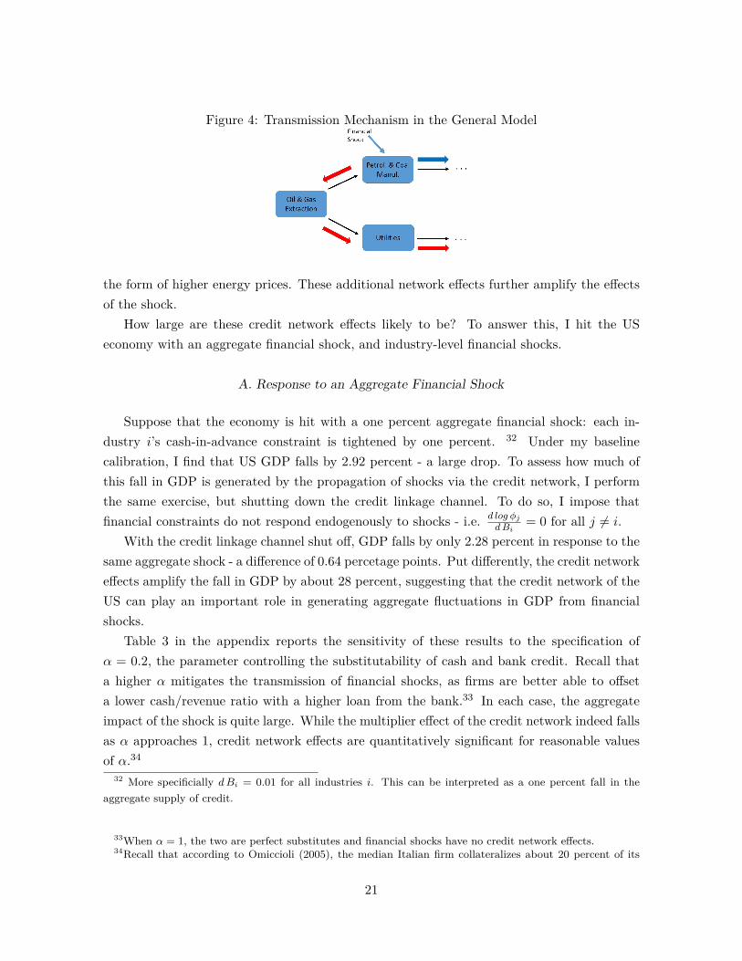
Figure 4: Transmission Mechanism in the General Model

the form of higher energy prices. These additional network effects further amplify the effectsof the shock.

How large are these credit network effects likely to be? To answer this, I hit the USeconomy with an aggregate financial shock, and industry-level financial shocks.

A. Response to an Aggregate Financial Shock

Suppose that the economy is hit with a one percent aggregate financial shock: each in-dustry i’s cash-in-advance constraint is tightened by one percent. 32 Under my baselinecalibration, I find that US GDP falls by 2.92 percent - a large drop. To assess how much ofthis fall in GDP is generated by the propagation of shocks via the credit network, I performthe same exercise, but shutting down the credit linkage channel. To do so, I impose thatfinancial constraints do not respond endogenously to shocks - i.e. d log φj

dBi= 0 for all j 6= i.

With the credit linkage channel shut off, GDP falls by only 2.28 percent in response to thesame aggregate shock - a difference of 0.64 percetage points. Put differently, the credit networkeffects amplify the fall in GDP by about 28 percent, suggesting that the credit network of theUS can play an important role in generating aggregate fluctuations in GDP from financialshocks.

Table 3 in the appendix reports the sensitivity of these results to the specification ofα = 0.2, the parameter controlling the substitutability of cash and bank credit. Recall thata higher α mitigates the transmission of financial shocks, as firms are better able to offseta lower cash/revenue ratio with a higher loan from the bank.33 In each case, the aggregateimpact of the shock is quite large. While the multiplier effect of the credit network indeed fallsas α approaches 1, credit network effects are quantitatively significant for reasonable valuesof α.34

32 More specificially dBi = 0.01 for all industries i. This can be interpreted as a one percent fall in theaggregate supply of credit.

33When α = 1, the two are perfect substitutes and financial shocks have no credit network effects.34Recall that according to Omiccioli (2005), the median Italian firm collateralizes about 20 percent of its

21

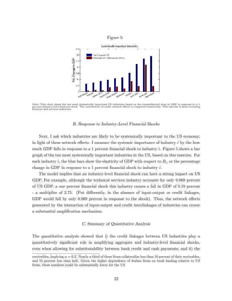
Figure 5:

Notes: This chart shows the ten most systemically important US industries based on the counterfactual drop in GDP in response to a 1percent industry-level financial shock. The contribution of credit network effects is computed numerically. This exercise is done excludingfinancial and services indsutries.

B. Response to Industry-Level Financial Shocks

Next, I ask which industries are likely to be systemically important to the US economy,in light of these network effects. I measure the systemic importance of industry i by the howmuch GDP falls in response to a 1 percent financial shock to industry i. Figure 5 shows a bargraph of the ten most systemically important industries in the US, based on this exercise. Foreach industry i, the blue bars show the elasticity of GDP with respect to Bi, or the percentagechange in GDP in response to a 1 percent financial shock to industry i.

The model implies that an industry-level financial shock can have a strong impact on USGDP. For example, although the technical services industry accounts for only 0.069 percentof US GDP, a one percent financial shock this industry causes a fall in GDP of 0.19 percent- a multiplier of 2.75. (Put differently, in the absence of input-output or credit linkages,GDP would fall by only 0.069 percent in response to the shock). Thus, the network effectsgenerated by the interaction of input-output and credit interlinkages of industries can createa substantial amplification mechanism.

C. Summary of Quantitative Analysis

The quantitative analysis showed that i) the credit linkages between US industries play aquantitatively significant role in amplifying aggregate and industry-level financial shocks,even when allowing for substitutability between bank credit and cash payments; and ii) the

receivables, implying α = 0.2. Nearly a third of these firms collateralize less than 10 percent of their receivables,and 55 percent less than half. Given the higher dependence of Italian firms on bank lending relative to USfirms, these numbers could be substantially lower for the US.

22

systemic importance of an industry depends on the input-output and credit network effectsof shocks. Therfore, an understanding of the role that credit linkages play in propagatingidiosyncratic shocks introduces a new notion of the systemic importance of firms or industriesbased on their place in the credit network.

D. Mapping the Model to the Data

In order to map the model to the data, I extend the static model to be a repeated cross-section. Let Xt, Nt, Bt, and zt denote the M -by-1 vectors of output growth, employmentgrowth, financial shocks, and productivity for each industry respectively, in quarter t. Thelog-linearized model yields closed-form expressions for how the output and employment ofeach industry respond to financial and productivity shocks. (These are derived in the onlineTechnical Appendix.)

Xt = GXBt +HXzt Nt = GNBt +HNzt (28)

TheM -by-M matrices GX and HX (GN and HN ) map industry-level financial and productiv-ity shocks, respectively, into output growth (employment growth), and capture the effects ofinput-output and credit interlinkages in propagating shocks across industries. The elementsof these matrices depend only on the model parameters, and therefore take their values frommy calibration.

I construct the observed, quarterly cyclical fluctuations in the output Xt and employmentNt of US industrial production industries using data from the Federal Reserve Board’s Indus-trial Production Indexes, which includes data on the output growth of these industries, andthe Bureau of Labor Statistics’ Quarterly Census of Employment and Wages, from which Iobserve the number of workers employed by each of these indutries. At the three-digit NAICSlevel there are 23 such industries.35 For each dataset, I take 1997 Q1 through 2013 Q4 as mysample period, and seasonally-adjust and de-trend each series. In the empirical analysis tofollow, I use this data and the expressions (28) to decompose observed cyclical fluctuationsinto various components.

V. Empirical Analyses35Hours worked is not directly available at this level of industry detail and this frequency.

23

In the empirical part of the paper, I use my theoretical framework to investigate whichshocks drive observed cyclical fluctuations in the US, once we account for the network effectscreated by credit and input-output linkages between industries. The framework is rich enoughto permit an empirical exploration of the sources of these fluctuations along two separatedimensions: the importance of productivity versus financial shocks, and that of aggregateversus idiosyncratic shocks.

The model allows one to disentagle the contribution of two supply-side shocks to observedfluctuations: financial and productivity shocks. Furthermore, the model allows for networkeffects to generate fluctuations in economic aggregates from idiosyncratic (industry-level)shocks. This permits a disctinction of the roles of idiosyncratic versus purely aggregateshocks in driving aggregate fluctuations. To decompose observed cyclical fluctuations intocomponents along these two dimensions, I use two methodological approaches. In the first,I identify shocks without imposing the structure of my model on the data; in the second, Iidentify shocks using a structural estimation.

First Method: Estimating Shocks without the Model

My first approach involves identifying financial and productivity shocks without imposing thestructure of my model on the data - the identifying assumptions are completely independentof the model. An added advantage of this method is that it permits the estimation of aresidual component of observed fluctuations - a component which is not explained by eithershock. However, the shocks estimated using this method are assumed to be common to allindustries.

A. Estimating financial shocksTo identify credit supply shocks to the US economy, I estimate an identified VAR using

a similar approach as Gilchrist and Zakrajsek (2011). To do this requires first constructing ameasure of bank-intermediated business lending.

I construct a measure of aggregate business lending by US financial intermediaries usingquarterly Call Report data collected by the FFIEC. To capture lending to the business sector,I use commercial and industrial loans outstanding.36 But as Gilchrist and Zakrajsek (2011)show, this type of on-balance sheet lending reacts to financial market disruptions only witha signficant lag. In contrast, a cyclically-sensitive component of bank lending is unusedcommitments, representing off-balance sheet lines of credit to businesses.37 While changes inunused commitments after a financial shock mostly reflect a tightening in the supply of lines

36This is a conservative estimate of bank lending to US firms.37The authors show that the contraction in unused loan commitments was concomitant with onset of the

financial crisis in 2007, while business loans outstanding contracted only with a lag of about four quarters.

24

of credit38, they could also reflect borrowers drawing down the unused portion of their linesof credit - a change in the demand for bank loans. To net out any demand-side changes inbank lending, I construct a quarterly measure of aggregate bank lending, called the businesslending capacity of the financial sector, as the sum of unused commitments and commercialand industrial loans outstanding in each quarter.39

To empirically identify credit supply shocks, I augment a standard VAR of macroeconomicand financial variables with the measure of business lending capacity, and the excess bondpremium of Gilchrist and Zakrajsek (2012) - a component of corporate credit spreads designedto capture changes in the risk-bearing capacity of financial intermediaries.40 The endogenousvariables included in the VAR, ordered recursively, are: (i) the log-difference of real businessfixed investment; (ii) the log-difference of real GDP; (iii) inflation as measured by the log-difference of the GDP price deflator; (iv) the quarterly average of the excess bond premium;(v) the log difference business lending capacity (vi) the quarterly (value-weighted) excess stockmarket return from CRSP; (vii) the ten-year (nominal) Treasury yield; and (viii) the effective(nominal) federal funds rate. The identifying assumption implied by this ordering is thatstock prices, the risk-free rate, and bank lending can react contemporaneously to shocks tothe excess bond premium, while real economic activity and inflation respond with a lag. Iestimate the VAR using two lags of each endogenous variable.

To map the orthogonalized innovations in the excess bond premium into the financialshocks Bt of my model, I make use of the impulse response function of business lendingcapacity. I thus construct my financial shocks as changes in the supply of bank lendingwhich arise due to innovations in the risk-bearing capacity of the financial sector, which areorthogonal to macroeconomic conditions. Figure 6 plots the time series of this shock.

Thus far, this procedure produced estimates of a financial shock which is common to allindustries. Yet shocks to credit availability may affect industries differentially depending ontheir dependence on external finance. To allow for this, I load the financial shocks Bt ontoeach industry based on a measure EFDi of the the industry’s external finance dependence,which I construct according to Rajan and Zingales (1995).41 Since the quantitative resultsdo not significantly change, the result reported hereafter are for financial shocks which load

38See Gilchrist and Zakrajsek (2011) for evidence.39To see why changes in this measure of business lending capacity mostly reflect supply-side changes, consider

the following example. Suppose that a business draws down an existing line of credit it has with its bank.This is recorded as a fall in unused commitments, but reflects an increase in demand for credit rather than acontraction in the supply of credit. However, the loan is now recorded as an on-balance sheet commercial orindustrial loan. Therefore, the fall in unused commitments is exactly offset by the increase in commercial andindustrial loans outstanding, leaving bank lending capacity unchanged. So this measure of business lendingcapacity is largely unresponsive to firms drawing down their lines of credit.

40I thank Simon Gilchrist for kindly sharing the excess bond premium data.41In this manner, I obtain a time-varying, industry-specific financial shock Bit which can be fed into the

model.Although they varies across industries in any given quarter, these shocks to each industry are perfectlycorrelated across time, and so should not be interpreted as idiosyncratic shocks.

25

Figure 6:

2002 2003 2004 2005 2006 2007 2008 2009 2010−10

−5

0

5

10

Pe

rce

nt C

ha

ng

e

Externally Estimated Financial and Productivity Shocks

Estimated credit supply shock

Utilization−adjusted TFP

Notes: This figure shows the series of quarter-to-quarter growth in utilization-adjusted TFP measure of Fernald (2012) and the creditsupply shocks, estimated as changes in the business lending capacity of the financial sector which are due to orthogonalized innovationsto the excess bond premium. Financial shocks were estimated using an identified VAR.. TFP data was obtained from the San FranciscoFed database.

equall onto all industries. Let Bt denote the M -by-1 vector of these shocks.

B. Estimating productivity shocksThe Federal Reserve Bank of San Francisco produces a quarterly series on TFP for the

US business sector, adjusted for variations in factor utilization, according to Fernald (2012).As such, this series is readily mapped into my model as an aggregate productivity shock zt.Figure 6 plots time series for this productivity shock. Let zt ≡ zt~1 denote the M -by-1 vectorof these shocks.

C. Decomposing Observed Fluctuations in Industrial Production

With the estimated shocks at hand, I use log-linearized expression (28) to decompose ob-served cyclical fluctuations in industrial production into components coming from the financialshocks, productivity shocks, and a residual.

Xt = GXBt +HX zt + εt (29)

Components GXBt and HX zt reflect how much of observed, industry-level fluctuations inindustrial output come from financial and productivity shocks, respectively, when I feed theestimated financial and productivity shocks Bt and zt through the model. εt is the componentof these fluctuations which is unexplained by either of these shocks.

I then feed these shocks into the model and perform a variance decomposition of aggregateindustrial production. To do this, note that the assumption Xt = GXBt +HXzt + εt implies

26

Table 1: Variance Decomposition of IP: 2001Q4:2007Q3

Share ofAggregate Volatility

Productivity Shocks 0.205

Financial Shocks 0.279

Residual 0.516

Notes: This table reports the results of the variance decomposition of the quarterly time series of aggregate industrial production overthe pre-recessionary period 2001 Q4 - 2007 Q3. Aggregate volatility is computed as the sample variance of observed aggregate industrialproduction. Financial shocks were estimated using an identified VAR, and capture quarterly credit supply shocks to the productive sector.Productivity shocks are estimated by Fernald (2012) as quarter-to-quarter, utilization-adjusted changes in TFP in the US, obtained fromthe San Francisco Fed database. The residual is the component of aggregate industrial production which is unexplained after these shocksare fed through the log-linearized model.

that output volatility can be decomposed in the following way, where ΣXX , ΣBB,Σzz, andΣεε denote the variance-covariance matrices of Xt, Bt, zt, and εt, respectively.42

ΣXX = GXΣBBG′X +HXΣzzH

′X + Σεε (30)

In addition, letting s denote the M -by-1 vector of industry shares of aggregate output duringthe median year of my sample, 2005, the volatility of aggregate industrial output - henceforthaggregate volatility - can be approximated by σ ≡ s′ΣXX s.43 Then the fraction of observed ag-gregate volatility generated by financial shocks, for example, is given by (s′GXΣBBG

′X s) /σ2.

This is derived in further detail in Appendix A4.The variance decomposition of output before 2007 is given in Table 1. In the period 2001

- 2007, productivity and financial shocks played a roughly equal role in generating cyclicalfluctuations, together accounting for half of observed aggregate volatility in US industrialproduction. The remaining half is unaccounted for by either type of shock.

However, the story is different for the Great Recession. Figure 7 plots the time seriesof aggregate industrial production during the Great Recession, as well as a simulation foreach of its components.44 These counterfactual series are constructed by feeding each of theestimated components through the model one at a time, and thus represents how aggregateindustrial production would have evolved in the absence of other shocks, beginning in 2007

42Implicit in this decomposition is the assumption that Bt,zt, and εt are orthogonal to each other.43 I find that, for the full sample period 1997Q1:2013Q4, aggregate volatility in industrial production is

about 0.19%. This is roughly in line with the findings of Foerster et al. (2011). If I compute growth ratesand aggregate volatility using the same scaling conventions as they, I find aggregate volatility to be about9.35 compared to their 8.8 for 1972-1983 and 3.6 for 1984-2007. The higher volatility that I get comes fromincluding the Great Recession in my sample period.

44The time series for observed aggregate IP is constructed from the cyclical component of IP growth. It isconstructed as an aggregate index of the observed industry-level growth rates.

27

Figure 7:

2007Q4 2008Q1 2008Q2 2008Q3 2008Q4 2009Q1 2009Q2 2009Q360

70

80

90

100

110

120

130

Index Level

Aggregate IP and Its Components

Observed Aggregate IP

Financial Component

Productivity Component

Residual

Notes: This figure shows the time series of aggregate industrial production and its components. Observed aggregate industrial productionis an index constructed from the de-trended, seasonally-adjusted industry-level quarter-to-quarter growth rates in the output of the23 industrial production industries at the three-digit NAICS level, obtained from FRB IP Indexes. Each of the other series depictcounterfactual indexes constructed from the respective components of the observed series, beginning in 2007 Q3, and represent howaggregate IP would have evolved in the absence of other shocks. Financial shocks were estimated using an identified VAR Productivityshocks are estimated by Fernald (2012) as quarter-to-quarter, utilization-adjusted changes in TFP in the US, obtained from the SanFrancisco Fed database.

Q3.During the recession, productivity shocks had virtually no adverse effects on industrial

production - in fact, they actually mitigated the downturn. Rather, financial shocks are themain culprit, accounting for two-thirds of the peak-to-trough drop in aggregate industrialproduction during the recession. The remaining one-third is not accounted for by eithershock. Furthermore, the credit network of these industries played a quantitatively significantrole during this period, amplifying the effects of the financial shocks by about 15% (i.e. adding3.98 percentage points to the peak-to-trough drop in the financial component of aggregateindustrial production).

Second Method: Structural Factor Analysis

With my second methodological approach, I empirically assess the relative contribution ofaggregate versus idiosyncratic shocks in generating cyclical fluctuations. This involves esti-mating the model using a structural factor approach similar to that of Foerster, Sarte, andWatson (2011)45, using data on the output and employment growth of US IP industries. Theprocedure involves two steps. I first use a log-linear approximation of the model to back-out the productivity and financial shocks to each industry required for the model to matchthe fluctuations in the output and employment data. Then, I use dynamic factor methods todecompose each of these shocks into an aggregate component and an idiosyncratic component.

45Foerster et al. (2011) allow only for productivity shocks in driving observed fluctuations.

28

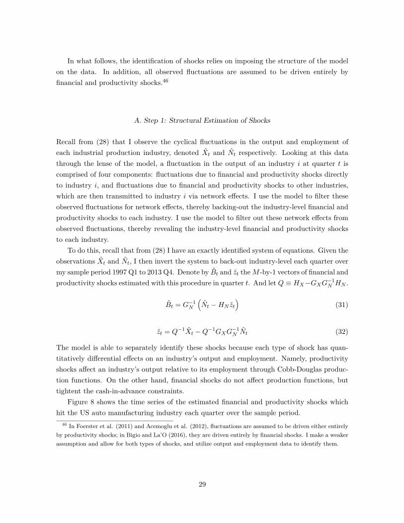
In what follows, the identification of shocks relies on imposing the structure of the modelon the data. In addition, all observed fluctuations are assumed to be driven entirely byfinancial and productivity shocks.46

A. Step 1: Structural Estimation of Shocks

Recall from (28) that I observe the cyclical fluctuations in the output and employment ofeach industrial production industry, denoted Xt and Nt respectively. Looking at this datathrough the lense of the model, a fluctuation in the output of an industry i at quarter t iscomprised of four components: fluctuations due to financial and productivity shocks directlyto industry i, and fluctuations due to financial and productivity shocks to other industries,which are then transmitted to industry i via network effects. I use the model to filter theseobserved fluctuations for network effects, thereby backing-out the industry-level financial andproductivity shocks to each industry. I use the model to filter out these network effects fromobserved fluctuations, thereby revealing the industry-level financial and productivity shocksto each industry.

To do this, recall that from (28) I have an exactly identified system of equations. Given theobservations Xt and Nt, I then invert the system to back-out industry-level each quarter overmy sample period 1997 Q1 to 2013 Q4. Denote by Bt and zt theM -by-1 vectors of financial andproductivity shocks estimated with this procedure in quarter t. And let Q ≡ HX−GXG−1

N HN .

Bt = G−1N

(Nt −HN zt

)(31)

zt = Q−1Xt −Q−1GXG−1N Nt (32)

The model is able to separately identify these shocks because each type of shock has quan-titatively differential effects on an industry’s output and employment. Namely, productivityshocks affect an industry’s output relative to its employment through Cobb-Douglas produc-tion functions. On the other hand, financial shocks do not affect production functions, buttightent the cash-in-advance constraints.

Figure 8 shows the time series of the estimated financial and productivity shocks whichhit the US auto manufacturing industry each quarter over the sample period.

46 In Foerster et al. (2011) and Acemoglu et al. (2012), fluctuations are assumed to be driven either entirelyby productivity shocks; in Bigio and La’O (2016), they are driven entirely by financial shocks. I make a weakerassumption and allow for both types of shocks, and utilize output and employment data to identify them.

29

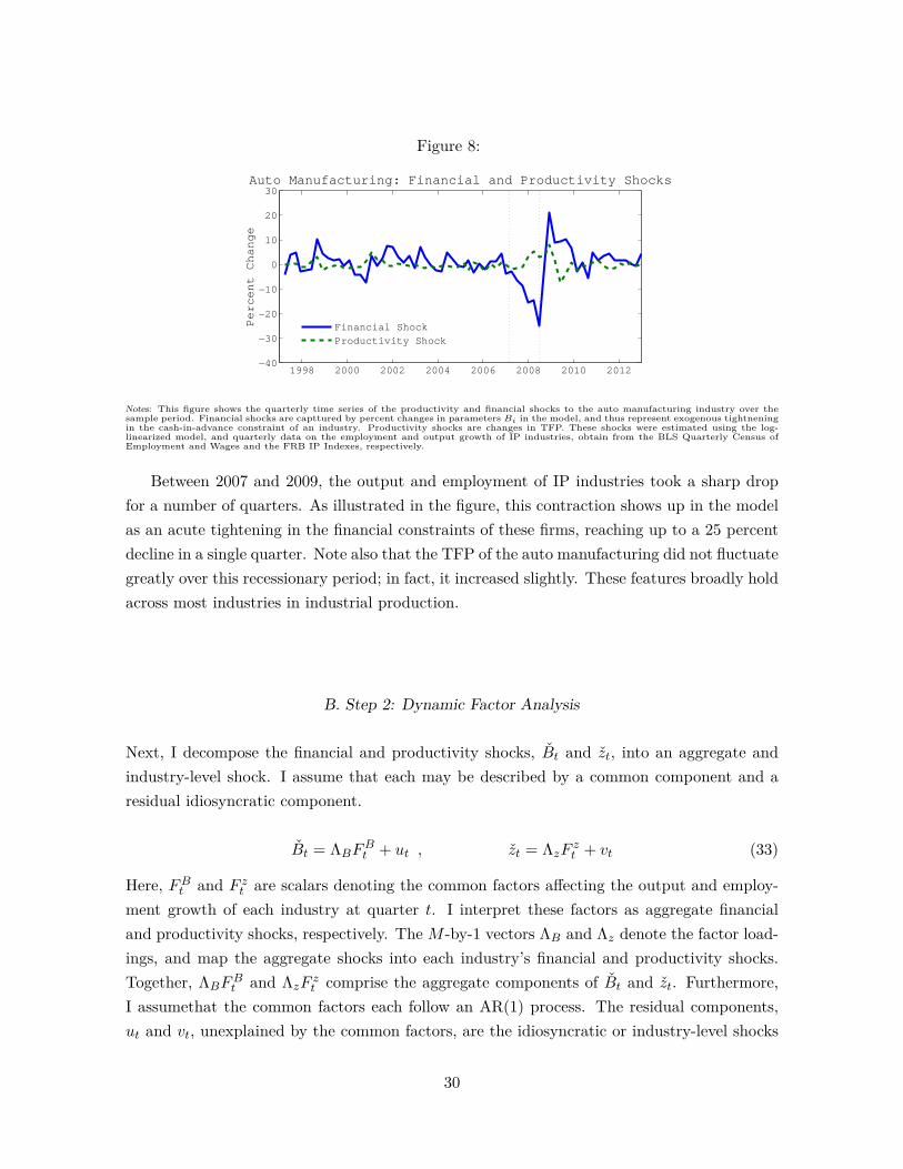
Figure 8:

1998 2000 2002 2004 2006 2008 2010 2012−40

−30

−20

−10

0

10

20

30

Pe

rce

nt

Ch

an

ge

Auto Manufacturing: Financial and Productivity Shocks

Financial Shock

Productivity Shock

Notes: This figure shows the quarterly time series of the productivity and financial shocks to the auto manufacturing industry over thesample period. Financial shocks are capttured by percent changes in parameters Bi in the model, and thus represent exogenous tightneningin the cash-in-advance constraint of an industry. Productivity shocks are changes in TFP. These shocks were estimated using the log-linearized model, and quarterly data on the employment and output growth of IP industries, obtain from the BLS Quarterly Census ofEmployment and Wages and the FRB IP Indexes, respectively.

Between 2007 and 2009, the output and employment of IP industries took a sharp dropfor a number of quarters. As illustrated in the figure, this contraction shows up in the modelas an acute tightening in the financial constraints of these firms, reaching up to a 25 percentdecline in a single quarter. Note also that the TFP of the auto manufacturing did not fluctuategreatly over this recessionary period; in fact, it increased slightly. These features broadly holdacross most industries in industrial production.

B. Step 2: Dynamic Factor Analysis

Next, I decompose the financial and productivity shocks, Bt and zt, into an aggregate andindustry-level shock. I assume that each may be described by a common component and aresidual idiosyncratic component.

Bt = ΛBFBt + ut , zt = ΛzF zt + vt (33)

Here, FBt and F zt are scalars denoting the common factors affecting the output and employ-ment growth of each industry at quarter t. I interpret these factors as aggregate financialand productivity shocks, respectively. The M -by-1 vectors ΛB and Λz denote the factor load-ings, and map the aggregate shocks into each industry’s financial and productivity shocks.Together, ΛBFBt and ΛzF zt comprise the aggregate components of Bt and zt. Furthermore,I assumethat the common factors each follow an AR(1) process. The residual components,ut and vt, unexplained by the common factors, are the idiosyncratic or industry-level shocks

30

Figure 9:

1998 2000 2002 2004 2006 2008 2010 2012−2

−1

0

1

2

3

4Excess Bond Premium and Aggregate Financial Shocks

Aggregate Financial Shock

Excess Bond Premium

Notes: This figure shows the time series of the excess bond premium of Gilchrist and Zakrajsek (2012) and the aggregate component of thefinancial shocks to industrial produciton industries estimated using the structural factor analysis of these industries’ quarterly output andemployment growth. The excess bond premium is a component of corporate credit spreads designed to capture changes in the risk-bearycapacity of the financial sector. This measure was obtain from Gilchrist and Zakrajsek (2012).

affecting each industry’s financial and productivity growth. (The dynamic factor model andits assumptions are described in more detail in Appendix A4.) Hence, I estimate two dynamicfactor models; one for the financial shocks Bt and one for the productivity shocks zt.47 Theaggregate component explain most of the financial shocks suffered by auto manufacturing.These features are fairly representative of those in other industries.

To gauge the external validity of the structural factor analysis, I compare the aggregatefinancial shocks to the excess bond premium.48 estimated using the model with a measureof the risk-bearing capacity of the US financial sector - namely, the excess bond premiumof Gilchrist and Zakrajsek (2012). Figure 9 plots the two series together. The negativecorrelation (-0.51) between the two indicates that the sharp drop in the supply of credit fromthe financial sector is picked up by model as a dramatic tightening in the financial constraintsof firms in IP. Hence the large aggregate financial shocks estimated by the structural factoranalysis is broadly reflective of the severe credit crunch that occurred during this period.

47 I use standard methods to estimate the model. To predict the factors, I use both a one-step predictionmethod and Kalman smoother. The Kalman smoother yields factors which explain more of the data. Since itutilizes more infortmation in predicting the factors, I use this method as my baseline. All subsequent reportedresults used the factors predicted using a Kalman smoother.

48Recall the excess bond premium of Gilchrist and Zakrajsek (2012) is a measure of the risk-bearing capacityof the financial sector.

31

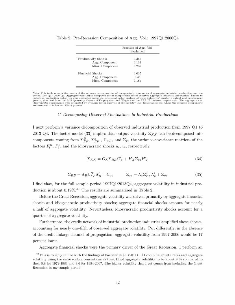
Table 2: Pre-Recession Composition of Agg. Vol.: 1997Q1:2006Q4

Fraction of Agg. Vol.Explained

Productivity Shocks 0.365Agg. Component 0.133Idios. Component 0.232

Financial Shocks 0.635Agg. Component 0.45Idios. Component 0.185

Notes: This table reports the results of the variance decomposition of the quarterly time series of aggregate industrial production over theperiod 1997 Q1 - 2006 Q4. Aggregate volatility is computed as the sample variance of observed aggregate industrial production. Shocks toindustrial produciton industries were estimated using the structural factor analysis of these industries’ quarterly output and employmentgrowth, obtained from the BLS Quarterly Census of Employment and Wages and the FRB IP Indexes, respectively. The aggregate andidiosycnratic components were estimated by dynamic factor analysis of the industry-level financial shocks, where the common componentsare assumed to follow an AR(1) process.

C. Decomposing Observed Fluctuations in Industrial Productions

I next perform a variance decomposition of observed industrial production from 1997 Q1 to2013 Q4. The factor model (33) implies that output volatility ΣXX can be decomposed intocomponents coming from ΣB

FF , ΣzFF , Σuu , and Σvv the variance-covariance matrices of the

factors FBt , F zt , and the idiosyncratic shocks ut, vt, respectively.

ΣXX = GXΣBBG′X +HXΣzzH

′X (34)

ΣBB = ΛBΣBFFΛ′B + Σuu Σzz = ΛzΣz

FFΛ′z + Σvv (35)

I find that, for the full sample period 1997Q1:2013Q4, aggregate volatility in industrial pro-duction is about 0.19%.49 The results are summarized in Table 2.

Before the Great Recession, aggregate volatility was driven primarily by aggregate financialshocks and idiosyncratic productivity shocks; aggregate financial shocks account for nearlya half of aggregate volatility. Nevertheless, idiosyncratic productivity shocks account for aquarter of aggregate volatility.

Furthermore, the credit network of industrial production industries amplified these shocks,accounting for nearly one-fifth of observed aggregate volatility. Put differently, in the absenceof the credit linkage channel of propagation, aggregate volatility from 1997-2006 would be 17percent lower.

Aggregate financial shocks were the primary driver of the Great Recession. I perform an49This is roughly in line with the findings of Foerster et al. (2011). If I compute growth rates and aggregate

volatility using the same scaling conventions as they, I find aggregate volatility to be about 9.35 compared totheir 8.8 for 1972-1983 and 3.6 for 1984-2007. The higher volatility that I get comes from including the GreatRecession in my sample period.

32

accounting exercise to evaluate how much of the peak-to-trough drop in aggregate industrialproduction over 2007Q4: 2009Q2 can be explained by each type of shock. For each quarterduring this period, I use the estimated shocks to decompose the drop in aggregate IP intocomponents arising from each type of shock. For each quarter, this yields a breakdown ofthe quarterly decline in aggregate IP across each shock. I then take a weighted sum of thesebreakdowns across quarters, with weights reflecting the share of the total fall in aggregate IPthat occurred each quarter. I thus measure how much of the total peak-to-trough decline inaggregate IP during the Great Recession can be accounted for by each type of shock.

I find that both aggregate and idiosyncratic productivity shocks were on average slightlypositive during this period. As such, changes in productivity did not contribute to the declinein aggregate IP during the recession. On the contrary, the observed movements in aggregateIP can be accounted for by financial shocks. I find that 73 percent of the drop in aggregateIP is due to an adverse aggregate financial shock. This is natural given the financial crisisthat occurred during the beginning of the recession.

Financial shocks explain all of the downward pressure on industrial production. Indeed,73 percent of the drop in aggregate IP is due to aggregate financial shocks. Of the remaining27 percent not explained by the aggregate financial shock, idiosyncratic financial shocks tothe three most systemically important industries can account for a sizable fraction.

Figure 10 depicts the relationship between industry-level financial shocks and an indus-try’s contribution to aggregate output, for industrial production industries during the GreatRecession. The horizontal axis plots the mean financial shock (including both the aggregateand idiosyncratic components) to each IP industry over the recessionary period; the verticalaxis the share of the peak-to-trough drop in aggregate output attributable to each industry.The plot is weighted by the measure of each industry’s systemic importance produced by myquantitative analysis in section IV.B, and are augmented with a least-squares line.

Large financial shocks to a few systemically important industries can explain the bulk ofthe decline in aggregate industrial production during the Great Recession. In fact, idiosyn-cratic shocks to the oil and coal products manufacturing, chemical products manufacturing,and auto manufacturing industries account for about 9 percent of the decline (or one-third ofthe decline unaccounted for by aggregate shocks), despite comprising only about 25 percent ofaggregate IP. This suggests that idiosynratic financial shocks to a few systemically importantindustries played a quantitatively significant role during the Great Recession.

In contrast, both the aggregate and idiosyncratic components of productivity shocks wereslightly positive during this period on average. As such, changes in productivity did notcontribute to the decline in aggregate IP during the recession.

33

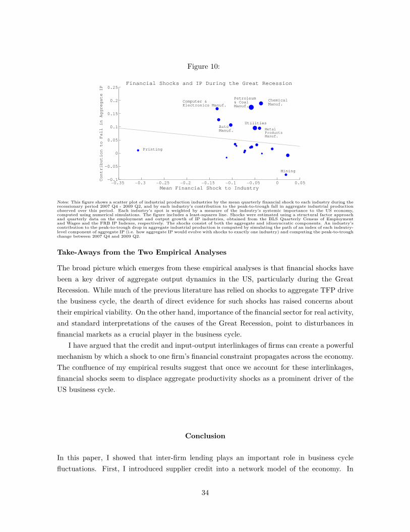
Figure 10:

−0.35 −0.3 −0.25 −0.2 −0.15 −0.1 −0.05 0 0.05−0.1

−0.05

0

0.05

0.1

0.15

0.2

0.25

Mean Financial Shock to Industry

Co

ntr

ibu

tion

to

Fa

ll in

Ag

gre

ga

te I

P

Financial Shocks and IP During the Great Recession

MetalProductsManuf.

Computer &Electronics Manuf.

ChemicalManuf.

Petroleum& CoalManuf.

AutoManuf.

Utilities

Printing

Mining

Notes: This figure shows a scatter plot of industrial production industries by the mean quarterly financial shock to each industry during therecessionary period 2007 Q4 - 2009 Q2, and by each industry’s contribution to the peak-to-trough fall in aggregate industrial productionobserved over this period. Each industry’s spot is weighted by a measure of the indsutry’s systemic importance to the US economy,computed using numerical simulations. The figure includes a least-squares line. Shocks were estimated using a structural factor approachand quarterly data on the employment and output growth of IP industries, obtained from the BLS Quarterly Census of Employmentand Wages and the FRB IP Indexes, respectively. The shocks consist of both the aggregate and idiosyncratic components. An industry’scontribution to the peak-to-trough drop in aggregate industrial production is computed by simulating the path of an index of each indsutry-level component of aggregate IP (i.e. how aggregate IP would evolve with shocks to exactly one industry) and computing the peak-to-troughchange between 2007 Q4 and 2009 Q2.

Take-Aways from the Two Empirical Analyses

The broad picture which emerges from these empirical analyses is that financial shocks havebeen a key driver of aggregate output dynamics in the US, particularly during the GreatRecession. While much of the previous literature has relied on shocks to aggregate TFP drivethe business cycle, the dearth of direct evidence for such shocks has raised concerns abouttheir empirical viability. On the other hand, importance of the financial sector for real activity,and standard interpretations of the causes of the Great Recession, point to disturbances infinancial markets as a crucial player in the business cycle.

I have argued that the credit and input-output interlinkages of firms can create a powerfulmechanism by which a shock to one firm’s financial constraint propagates across the economy.The confluence of my empirical results suggest that once we account for these interlinkages,financial shocks seem to displace aggregate productivity shocks as a prominent driver of theUS business cycle.

Conclusion

In this paper, I showed that inter-firm lending plays an important role in business cyclefluctuations. First, I introduced supplier credit into a network model of the economy. In

34

this model, a shock to one firm’s liquid funds reduces its ability to make payments to itssuppliers. The credit linkages between firms and their suppliers thus propagate the firm-levelshock across the network, amplifying its aggregate effects. Thus, the endogenous responsein cash-in-advance constraints to financial shocks is crucial for how the economy behaves inresponse to financial shock.

To evaluate the model quantitatively, I constructed a proxy of the credit linkages betweenUS industries by combining firm-level balance sheet data and industry-level input-output data.Counterfactual exercises reveal that these interlinkages can produce a powerful amplificationmechanism of industry-level shocks.

Finally, I used the model to investigate which shocks drive the US business cycle when weaccount for the linkages between industries. To do so, I took two approaches to identifyingshocks. In the first, I identified shocks without the use of my model, by estimating an iden-tified VAR. In the second, I constructed shocks using my model, and used factor methods todecompose them into aggregate and idiosyncratic components. Feeding these shocks thoughthe model showed financial shocks to be a key driver of aggregate fluctuations, particularlyduring the Great Recession, and productivity shocks to play only a minor role. Thus, account-ing for the role that credit and input-output interlinkages play helps to capture the empiricalimportance of financial shocks in US business cycle fluctuations.

References

[1] Acemoglu, Daron, Ufuk Akcigit, and William Kerr (2015), “Networks and the Macroeconomy: An Em-pirical Exploration”, Unpublished manuscript.

[2] Acemoglu, Daron, Vasco Carvalho, Asuman Ozdaglar, and Alireza Tahbaz-Salehi (2012), “The NetworkOrigins of Aggregate Fluctuations”, Econometrica, 80(5): 1977-2016.

[3] Atalay, Enghin (2014), “How Important Are Secotral Shocks?”, Unpublished manuscript.

[4] Barrot, Jean-Noel (2015), “Trade Credit and Industry Dynamics: Evidence from Trucking Firms”, Jour-nal of Finance.

[5] Barrot, Jean-Noel and Julien Sauvagnat (2014),“Input Specificity and Propagation of Idiosyncratic Shocksin Production Networks”, Unpublished manuscript.

[6] Basu, Susanto and John Fernald (1999), “Why is Productivity Procyclical? Why Do We Care?” FederalReserve Board of Governors, International Finance Discussion Papers, 638

[7] Baqaee, David Rezza (2016), “Cascading Failures in Production Networks”, Unpublished manuscript.

[8] Bernanke, Ben and Mark Gertler (1995), “Inside the Black Box: The Credit Channel of Monetary PolicyTransmission”, Journal of Economic Perspectives, 9(4), 27-48

35

[9] Bernanke, Ben, Mark Gertler, and Simon Gilchrist (1999), “The Financial Accelerator in a QuantitativeBusiness Cycle Framework”,

[10] Bigio, Saki and Jennifer La’O (2016), “Financial Frictions in Production Networks”, Unpublishedmanuscript.

[11] Boissay, Frederic (2006) “Credit Chains and the Propagation of Financial Distress”, Unpublishedmanuscript, Working Paper Series 573, ECB.

[12] Boissay, Frederic and Reint Gropp (2012), “Payment Defaults and Interfirm Liquidity Provision”, Reviewof Finance, 17(6), 1853-1894.

[13] Burkart, Mike and Tore Ellingson (2004), “In-Kind Finance: A Theory of Trade Credit”, AmericanEconomic Review, 94(3), 569-590.

[14] Cardoso-Lecourtois, Miguel (2004), “Chain Reactions, Trade Credit, and the Business Cycle”, Econo-metric Society 2004 North American Summer Meetings 331.

[15] Carvalho, Vasco and Xavier Gabaix (2013), “The Great Diversification and its Undoing”, AmericanEconomic Review, 103(5), 1697-1727.

[16] Conley, Timothy and Bill Dupor (2003), “A Spatial Analysis of Sectoral Complementarities”, Journal ofPolitical Economy, 111(2), 311-352.

[17] Cunat, Vicente (2006), “Trade Credit: Suppliers and Debt Collectors and Insurance Providers”, Reviewof Financial Studies, 20(2), 491-527.

[18] Delli Gatti, Domenico, Mauro Gellagati, Bruce Greenwald, Alberto Russo, and Joseph E. Stiglitz (2007),“The Financial Accelerator in and Evolving Credit Network”, Journal of Economic Dynamics and Control,34(9), 1627-1650.

[19] Demirguc-Kunt, Asli and Vojislav Maksimovic (2001), “Firms as Financial Intermediaries: Evidence fromTrade Credit Data” Unpublished manuscript, World Bank.

[20] Di Giovanni, Julian, Andrei A. Levchenko, and Isabelle Mejean (2014), “Firms, Destinations, and Ag-gregate Fluctuations”, Econometrica, 82(4), 1303-1340.

[21] Dupor, Bill (1999), “Aggregation and Irrelevance in Multi-Sector Models”, Journal of Monetary Eco-nomics, 43(2), 391-409.

[22] Fisman, Raymond and Inessa Love (2003), “Trade Credit, Financial Intermediary Development, andIndustry Growth”, Journal of Finance, 58(1), 353-374.

[23] Foerster, Andrew T., Pierre-Daniel Sarte, and Mark W. Watson (2011), “Sectoral versus AggregateShocks: A Structural Factor Analysis of Industrial Production”, Journal of Political Economy, 119(1),1-38.

[24] Frank, Murray and Vojislav Maksimovic (2005), “Trade Credit, Collateral, and Adverse Selection”, Un-published manuscript. University of Maryland.

[25] Gabaix, Xavier (2011), “The Granular Origins of Aggregate Fluctuations”, Econometrica, 79(3), 733-772.

[26] Gilchrist, Simon and Egon Zakrajsek (2011), “Bank Lending and Credit Supply Shocks”, Approaches tothe Evolving World Economy. The Proceedings of the 16th World Congress of the International EconomicAssociation Vol. III: , 102(4), 1962-1720.

36

[27] Gilchrist, Simon and Egon Zakrajsek (2012), “Credit Spreads and Business Cycle Fluctuations”, AmericanEconomic Review, 102(4), 1962-1720.

[28] Horvath, Michael (1998), “Cyclicality and Sectoral Linkages: Aggregate Fluctuations from IndependentSectoral Shocks”, Review of Economic Dynamics, 1(4), 781-808.

[29] Horvath, Michael (2000), “Sectoral Shocks and Aggregate Fluctuations”, Journal of Monetary Economics,45(1), 69-106.

[30] Jermann, Urban and Vincenzo Quadrini (2012), “Macroeconomic Effects of Financial Shocks”, AmericanEconomic Review, 102(1): 238-271.

[31] Jacobson, Tor and Erik von Schedvin (2015), “Trade Credit and the Propagation of Corporate Failure”,Econometrica, 83(4), 1315-1371.

[32] Kalemli-Ozcan, Sebnem, Se-Jik Kim, Hyun-Song Shin, Bent E. Sorensen, and Sevcan Yesiltas (2013),“Financial Shocks in Production Chains”, Unpublished manuscript.

[33] Kiyotaki, Nobuhiro and John and Moore (1997) “Credit Chains”, Unpublished manuscript.

[34] Luo, Shaowen (2016), “Propagation of Financial Shocks in an Input-Output Economy with Trade andFinancial Linkages of Firms”, Unpublished manuscript.

[35] Petersen, Mitchell A. and Raghuram G. Rajan (1997), “Trade Credit: Theories and Evidence”, Reviewof Financial Studies, 10(3), 661-691.

[36] Raddatz, Claudio (2010), “Credit Chains and Sectoral Comovement: Does the Use of Trade CreditAmplify Sectoral Shocks?”, Review of Economics and Statistics, 92(4), 985-1003.

[37] Rajan, Raghuram G. and Luigi Zingales (1998), “Financial Dependence and Growth”, American Eco-nomics Review, 88(3), 559-586.

[38] Shea, John (2002), “Complementarities and Comovements”, Journal of Money, Credit, and Banking,34(2), 412-433.

[39] Stella, Andrea (2015) “Firm Dynamics and the Origins of Aggregate Fluctuations”, Journal of EconomicDynamics and Control, 55(), 71-88.

Appendix

A1. Demand for Trade Credit

Recall that the tightness of firm i’s cash-in-advance constraint is given by

χi ≡bipixi

+ τi−1pixi︸ ︷︷ ︸

debt/revenue ratio

+ 1− τipixi︸ ︷︷ ︸

cash/revenue ratio

Firm i’s problem is to choose its input purchases and trade credit borrowing to maximize itsprofits, subject to its cash-in-advance constraint. Recall that competition amongst suppliers

37

forces each firm to offer the maximum trade credit allowed by the borrowing constraint.Therefore, firm i takes τi as given.

maxni, xi−1, τi−1

pixi − wni − pi−1xi−1

s.t. wni + pixi−1 ≤ χi(τi−1)pixi

τi−1 ≤ θipixi

Notice that in general, there is a tradeoff to taking more trade credit (i.e. to increasing τi−1).A higher τi−1 relaxes firm i’s cash-in-advance constraint, allowing it to purchase more inputsceteris paribus. But a higher τi−1 may also tighten its supplier’s cash in advance constraint,causing the price of its intermediate good pi−1 to increase.

Let τ∗i−1 denote the optimal amount of trade credit borrowing. We can solve for optimalτ∗i−1 separately from ni and xi−1. In particular, there are three relevant cases.

Case 1) If both i and i−1 are unconstrained in equilibrium, then there is no tradeoff to firmi taking marginally more τi−1. So there is a continuum of τi−1 between which firm i is indif-ferent: the set of all τi−1 such that both firm i and firm i−1 are unconstrained in equilibrium,i.e. χi, χi−1 < 1. Without loss of generality, we can take τ∗i−1 = min τi−1| χi, χi−1 < 1.

Case 2) If i is unconstrained in equilibrium, but i− 1 is constrained in equilibrium, thenthe tradeoff mentioned above applies. The optimal τi−1 will be the minimum such that i’scash-in-advance constraint is not binding. Any τi−1 > τ∗i−1 will further constrain supplieri− 1, and therefore i will face a higher input price pi−1. And any τi−1 < τ∗i−1 will mean thatfirm i will be constrained in equilibrium and will have to reduce production.

Case 3) If firm i is constrained in equilibrium, τ∗i−1 is the maximum allowable by the tradecredit borrowing constraint: τ∗i−1 = θipixi. To see this, first recall that firm i actually consistsof a continuum of identical firms with CRS production. Being constrained, each individualfirm has an incentive to take the maximum amount of trade credit. They do not internalizethe fact that, when all firms do this, they may increase the price pi−1 of inputs that theyface. Therefore, even if there is a τi−1 < θipixi such that industry-wide profits will be higher(taking into account tradeoff of lower input price pi−1), these firms are unable to coordinateon that τi−1. Thus, in any equilibrium in which firm i is constrained (i.e. its cash-in-advanceconstraint is binding), the trade credit borrowing constraints bind and τi−1 = θipixi.

Given its choice of τ∗i−1, firm i then chooses its inputs to solve:maxni, xi−1

pixi − wni − pi−1xi−1

s.t. wni + pixi−1 ≤ χi(τ∗i−1)pixi

A2. Proof of Amplification

From the definitions of χi and φi, we have

38

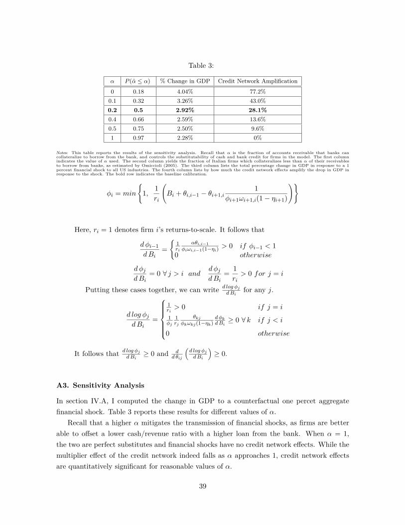
Table 3:

α P (α ≤ α) % Change in GDP Credit Network Amplification

0 0.18 4.04% 77.2%0.1 0.32 3.26% 43.0%0.2 0.5 2.92% 28.1%0.4 0.66 2.59% 13.6%0.5 0.75 2.50% 9.6%1 0.97 2.28% 0%

Notes: This table reports the results of the sensitivity analysis. Recall that α is the fraction of accounts receivable that banks cancollateralize to borrow from the bank, and controls the substitutability of cash and bank credit for firms in the model. The first columnindicates the value of α used. The second column yields the fraction of Italian firms which collateralizes less than α of their receivablesto borrow from banks, as estimated by Omiccioli (2005). The third column lists the total percentage change in GDP in response to a 1percent financial shock to all US industries. The fourth column lists by how much the credit network effects amplify the drop in GDP inresponse to the shock. The bold row indicates the baseline calibration.

φi = min

1, 1

ri

(Bi + θi,i−1 − θi+1,i

1φi+1ωi+1,i(1− ηi+1)

)

Here, ri = 1 denotes firm i’s returns-to-scale. It follows that

dφi−1dBi

=

1ri

αθi,i−1φiωi,i−1(1−ηi) > 0 if φi−1 < 1

0 otherwise

d φjdBi

= 0 ∀ j > i anddφjdBi

= 1ri> 0 for j = i

Putting these cases together, we can write d log φjdBi

for any j.

d log φjdBi

=

1ri> 0 if j = i

1φj

1rj

θkjφkωkj(1−ηk)

d φkdBi≥ 0 ∀ k if j < i

0 otherwise

It follows that d log φjdBi

≥ 0 and dd θij

(d log φjdBi

)≥ 0.

A3. Sensitivity Analysis

In section IV.A, I computed the change in GDP to a counterfactual one percet aggregatefinancial shock. Table 3 reports these results for different values of α.

Recall that a higher α mitigates the transmission of financial shocks, as firms are betterable to offset a lower cash/revenue ratio with a higher loan from the bank. When α = 1,the two are perfect substitutes and financial shocks have no credit network effects. While themultiplier effect of the credit network indeed falls as α approaches 1, credit network effectsare quantitatively significant for reasonable values of α.

39

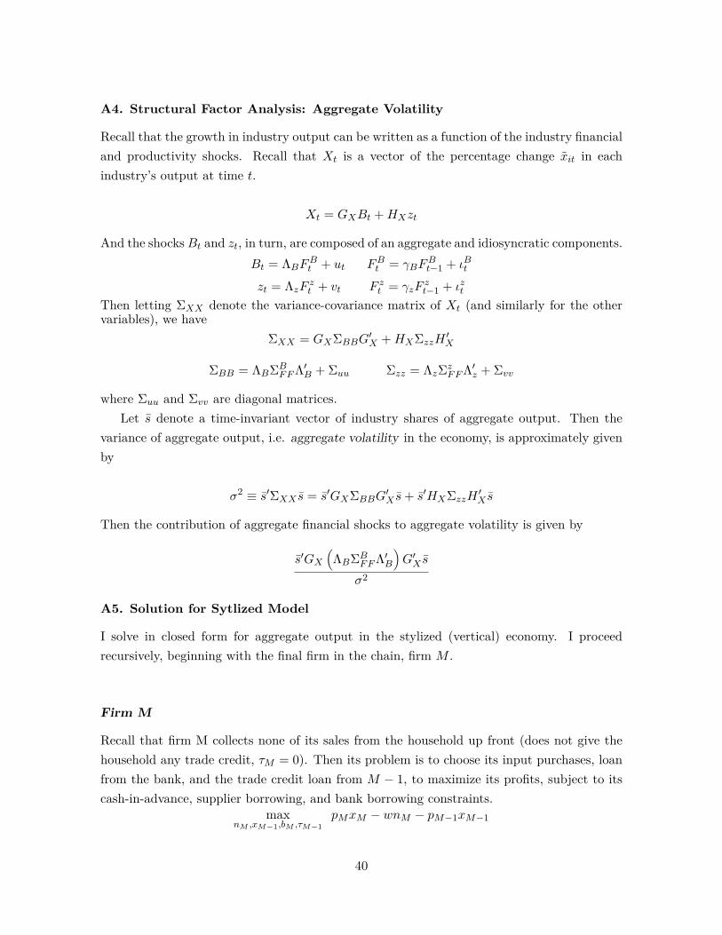
A4. Structural Factor Analysis: Aggregate Volatility

Recall that the growth in industry output can be written as a function of the industry financialand productivity shocks. Recall that Xt is a vector of the percentage change xit in eachindustry’s output at time t.

Xt = GXBt +HXzt

And the shocksBt and zt, in turn, are composed of an aggregate and idiosyncratic components.Bt = ΛBFBt + ut FBt = γBF

Bt−1 + ιBt

zt = ΛzF zt + vt F zt = γzFzt−1 + ιzt

Then letting ΣXX denote the variance-covariance matrix of Xt (and similarly for the othervariables), we have

ΣXX = GXΣBBG′X +HXΣzzH

′X

ΣBB = ΛBΣBFFΛ′B + Σuu Σzz = ΛzΣz

FFΛ′z + Σvv

where Σuu and Σvv are diagonal matrices.Let s denote a time-invariant vector of industry shares of aggregate output. Then the

variance of aggregate output, i.e. aggregate volatility in the economy, is approximately givenby

σ2 ≡ s′ΣXX s = s′GXΣBBG′X s+ s′HXΣzzH

′X s

Then the contribution of aggregate financial shocks to aggregate volatility is given by

s′GX(ΛBΣB

FFΛ′B)G′X s

σ2

A5. Solution for Sytlized Model

I solve in closed form for aggregate output in the stylized (vertical) economy. I proceedrecursively, beginning with the final firm in the chain, firm M .

Firm M

Recall that firm M collects none of its sales from the household up front (does not give thehousehold any trade credit, τM = 0). Then its problem is to choose its input purchases, loanfrom the bank, and the trade credit loan from M − 1, to maximize its profits, subject to itscash-in-advance, supplier borrowing, and bank borrowing constraints.

maxnM ,xM−1,bM ,τM−1

pMxM − wnM − pM−1xM−1

40

s.t. wnM + pM−1xM−1 ≤ bM + τM−1 + pMxM − τMbM ≤ BMpMxM + ατM

τM−1pM−1xM−1 ≤ θMpMxM

We can combine the constraints to re-write the problem.max

nM ,xM−1,bM ,τM−1pMxM − wnM − pM−1xM−1

s.t. wnM + pM−1xM−1 ≤ χMpMxMwhere χM = τ∗M−1

pMxM+ BM . Here, τ∗M−1 denotes firm M’s choice of trade credit borrowing,

based on the arguments given in Appendix A1. (Notice that when firm M is constrained,χM = θM,M−1 +BM ).If firm M is unconstrained in equilibrium, then the optimality conditions equate themarginal cost of each type of input with the marginal revenue.

w = ηMpMxMnM

pM−1 = (1− ηM )pMxMxM−1

(36)

Firm M’s expenditure in inputs is then

wnM + pM−1xM−1 = (ηM + (1− ηM )) pMxM (37)

Therefore, firm M is then unconstrained in equilibrium if and only if its expenditure at itsunconstrained optimum is less than its liquidity at this optimum.

pMxM < χMpMxM i.e. χM > 1 (38)

If firm M is constrained in equilibrium, then its binding cash-in-advance pins down itslevel of output. The only choice left to make is how much labor to hire nM versus howmuch intermediate goods xM−1 to purchase, given its level of output xM . Because χM isindependent of M’s choice of nM and xM−1, the problem of maximizing profits subject to thebinding cash-in-advance is equivalent to minimizing its expenditure nM + xM−1 subject toproducing xM . Thus, it solves the following cost-minimization problem.

minnM , xM−1 wnM + pM−1xM−1

s.t. xM = zMnηMM x

(1−ηM )M−1

Then firm M’s optimality condition equates the ratio of expenditure on each input with theratio of each input’s share in production.

wnMpM−1xM−1

= ηM(1− ηM ) (39)

Using this, we can rewrite M’s binding cash-in-advance as

wnM

(1 + (1− ηM )

ηM

)= χMpMxM (40)

41

Rearranging yields

w = ηMχMpMxMnM

(41)

Combining (41) with its analog (36) in the unconstrained case, we can see that

• if χM > rM (i.e. if firm i is unconstrained in equilibrium)

w = ηMpMxMnM

• otherwise

w = ηMχMpMxMnM

These two cases imply that we can write the optimality condition as

w = φMηMpMxMnM

(42)

φM ≡ min 1, χM represents the distortion in firm M’s optimal labor usage due to its cash-in-advance. Financial frictions introduce wedge between firm’s marginal benefit and cost ofproduction. The wedge between these two objects is increasing in the tightness χM of M’sconstraint, and decreasing in the returns-to-scale of firm M’s production function.

Firm M-1

Given firm M’s solution, we can proceed to firm M-1’s problem.

maxnM−1,xM−2 pM−1xM−1 − wnM−1 − pM−2xM−2

s.t. wnM−1 + pM−2xM−2 ≤ χM−1pM−1xM−1

where

χM−1 =τ∗M−2

pM−1xM−1+BM−1 + 1− (1− α) τM

pM−1xM−1

42

Here, τ∗M−2 denotes firm M-1’s optimal choice of trade credit borrowing. Again, if the firm’strade credit borrowing constraint binds in equilibrium, then χM−1 = θM−1 +BM−1 + 1− (1−α) τM

pM−1xM−1. If firms’ trade credit borrowing constraints bind in equilibrium, then

χM−1 = θM−1 +BM−1 + 1− (1− α) θMpMxMpM−1xM−1

And ( ?? ) and (?? ) imply that pMxMpM−1xM−1

= 1φMωM,M−1(1−ηM ) . Therefore,

χM−1 = θM−1 +BM−1 + 1− α θMφM (1− ηM )

Since φM is given by ( ?? ), this is a closed-form expression for χM−1. Note that, sinceφM depends on χM , χM−1 is an increasing function of χM ; this interdependence of cash-in-advances comes from the trade credit relationship between M and M-1.

Given χM−1, the solution to firm M-1’s problem takes the same form as that of firm M.(Note that χM−1 does not depend directly on M-1’s choice of nM−1 versus xM−2. Therefore,when constrained in equilibrium, M-1 will solve the analogous cost-minimization problem asM to maximize profits.) The cash-in-advance places a wedge φM−1 between the marginalbenefit of hiring labor and the marginal cost

w = φM−1ηM−1pM−1xM−1nM−1

Given the above expressions for χM−1 and χM , the the wedge φM−1 = min1, χM−1 is aclosed-form expression.Equilibrium

Each other firm’s problem is symmetric. Continuing recursively, I obtain the closed-formsolution for each firm. To summarize, I have, for each firm i

w = φiηipixini

where

φi = min1, χi and χi = Bi + θi + 1− θi+11

φi+1ωi,i−1(1− ηi)

Market clearing conditions are given by

C = Y ≡ xM , N =M∑i=1

ni

Given these expressions, the task is to write each ni as a function of aggregate outputxM , starting with firm M-1. From the firm optimality conditions, we have the following three

43

expressions:

wnM−1 = φM−1ηM−1pM−1xM−1, wnM = φMηMpMxM , pM−1xM−1 = wnM(1− ηM )ηM

Combining these yields nM−1 as a function of xM .

wnM−1 = φMφM−1ηM−1ωM,M−1(1− ηM )pMxM

Continuing recursively, we can write ni as a function of xM , for each i.

wni = pMxM

M∏j=i

φj

M−1∏j=i

ωj+1,j(1− ηj)

ηi (43)

The household’s preferences and optimality conditions imply

w = V ′(N)U ′(xM ) = xM (44)

Let good M be the numeraire. Combining (44) with (43) yields a closed-form expression foreach firm’s labor use.

ni = ηi

M∏j=i+

ωj,j−1(1− ηj)φj (45)

By recursively plugging in the production functions into one another, we can obtain aggregateoutput as a function of the labor use of each firm, where δM−i ≡

∏i−1j=0(1− ηM−j).

Y =(M−1∏i=0

zδM−iM−i

)(M−1∏i=0

nηM−iδM−iM−i

)(46)

Then combining (46) and (45) yields a closed-form expression for aggregate output (12).

44