The origin of coherence in hydrodynamical turbulence

Physica A 176 (1991) 241-296 North-Holland

THE ORIGIN OF COHERENCE IN HYDRODYNAMICAL TURBULENCE

E. LEVICH Physics Department, City College of the City University of New York, New York, NY 10031, USA and Benjamin Levich Center for Turbulence Research, ORMA T Industries Ltd., P. 0. Box 68, Yavne, Israel

L. SHTILMAN Department of Fluid Mechanics and Heat Transfer, Faculty of Engineering, Tel-A viv University, Israel

A.V. TUR Space Research hlstitute, Academy of Sciences, Moscow l 17810, USSR and Benjamh~ Levich Center for Tmbulence Re~earch, ORMA T htdustrie~ Ltd., P. 0. BoA" 68, Yavne, Israel

Received 4 January 1991

It is shown that the energy transfer to small scales turbulence necessarily requires a specific phase coherence of helicity-associated fluctuations. It follows that this coherence is a sufficient cause of turbulence intermittency in physical space, while both phase coherence and intermittency are consequences of the inviscid conservation of the topology of the vorticity field, in particular the helicity.

An important conclusion arrived at is that a perturbation of this coherence in the interiai range results in destruction of the vortex-line stretching mechanism and reduction or, finally, termination of turbulence production at small scales. Such phase reshuffling should cost negligible energy for high Reynolds number turbulent flows. The destruction of coherence can be achieved by a mere reshuffling of the phases connected with the related orientation of vorticity elements. Thus a possibility for practical turbulence control and drag reduction is indicated by the theory.

Theories of turbulence or modelling schemes based on closures, or more elaborate assumptions, such as the renormalization group theory, which by construction are phase independent, do not account for phase coherence and subsequent intermitt~i~cy and arc necessarily and fundamentally insufficient to describe this phenomenon.

It is shown that perturbations ef the vortex-line stretching mechanism may lead to an anomalous accumulation of helicity and a subsequent generation of large scale coherent vortices. Such organization of turbulence is asserted to be generic for the birth of large v~rtices in atmospheric phenomena.

The theory is shown to be in excellent agreement with extensive numerical simulations. Experimental data are briefly discussed.

0378-4371/91/$03.50 (~) 1991 - Elsevier Science Publishers B.V. (North-Holland)

242 E. Levich et al. / Origin of coherence in hydrodynamical turbulence

1. Introduction

Turbulence in fluids is often thought of as chaos with all possible dynamical degrees of freedom excited. Such perception is quite misguiding and should fade away. In its turn, turbulence emerges as a sublime and delicately organized state, a pattern of complexity and beauty where coherent and chaotic elements are logically and precisely intertwined.

Coherence in turbulence appears to follow from natural laws and is more general than any particular fluid mechanical aspect. Specifically at its origin is a balanced competition between the tendency of topological organization to be conserved, as is required by conservative (inviscid) dynamics, and the entropy growth, as is required by the second law of thermodynamics and procured by the energy transfer to small scales and subsequent viscous dissipation. What happens is that the turbulent machine is fed with low entropy energy at large scales and that by means of the nonlinear cascade mechanism it is transferred to small viscous scales and there spewed out into heat in exactly the same amount, but now endowed with a high entropy. This getting rid of high entropy sustains a weak topological order, which is a state of relatively low entropy, at large scales of turbulence. Moreover, the mechanism of energy transfer requires quite a specific coherence at all intermediate scales of turbulent motion.

It is this very presence of weak order, of latent coherence of certain degrees of freedom, which allows one to think of the possibility of turbulence control. Indeed, what would happen with turbulence if an external perturbation destroys this specific coherence? The answer is surprising and yet inescapable. If this latent coherence is disrupted, turbulence as it is known to us would cease to exist. The energy flow to small scales from the large energy containing scales would decrease, or ultimately terminate, and hence energy would stay, or in presence of energy injecting sources start to accumulate, at large scales. This process can be interpreted best as an instability at large scales of turbulence leading to a metamorphosis of the latent parental coherence into a tangible energy containing coherence. It is plausible that this process is related to coherent vortices observed as robust coherent structures (CS) in turbulent shear flows.

At least theoretically speaking, perturbations capable of greatly reducing developed turbulence and ultimately terminating it, would be cheap in terms of energy cost, since the ones required by the theory do not have to work systematically upon fluid elements, but rather rotate them at small scales, as we shall see shortly. One is profoundly amazed at the fragility of turbulence and the sensitive nature of its organization. Indeed, what a far cry from the chaotic unpredictability of fluid motion with which turbulence is usually associated! And yet theory and subsequent numerical experiment inexorably do not allow

E. Levich et al. / Origin of coherence in hydrodynamical turbulence 243

for any other alternative. Purely chaotic turbulence appears incompatible with the physics and mathematics imposed by the basic Navier-Stokes equation.

To understand and to observe the coherent nature of turbulence requires a penetration into its fine structure where it lies buried and dormant; to be sure this would not have been possible if not for numerical experiments carried ou" on supercomputers. Laboratory experimentation has yet to catch up with many aspects of turbulence structure, such as topological aspects requiring three- dimensional measurements, readily available from simulation of turb,.dPnt flows and called for by theoretical deductions.

Considerable empirical data, which in the last few decades have been pointing at the possibility of turbulence reduction and harnessing but hitherto were often seen as inexplicable extravaganza on the part of this intractable phenomenon, are suddenly cleared up and, at least in part, explained with some ease and rationality in the framework of the present theory as a partial destruction of sublime topological coherence.

1.1. Historical background

From the time of the classical works by Reynolds (1885), turbulence has been perceived as fluctuative motions in fluids involving all possible macro- scopic scales in space and time. These motions at various scales are all coupled to each other by means of the nonlinear interacting term in the Navier-Stokes (NS) equation. The energy for fluctuative motions is taken or as is usually said injected from the mean flow serving as a source, at large scales, and being dissipated at very small scales due to the molecular viscosity term in the NS equation. The competition between the nonlinear coupling and linear dissipation term is characterized by the value of Re = OchLch/V, where Vch and Lch are characteristic velocity and length scale, respectively, and v is the molecular viscosity. Thus fluctuative turbulent motion serves in this picture as a sink for the mean flow energy, and the cause for the energy losses. The more energy is transported from the mean flow to turbulent motion, the more energy is lost into heat.

This concept culminated in the empirical theories of Prandtl and von Karman enlarging on Reynolds' ideas, in these it was postulated that for an arbitrary turbulent flow the whole sum of action of fluctuative turbulent motion upon the mean flow can be viewed as an effective renormalization of the molecular viscosity into an eddy or turbulent viscosity v T, by orders of magnitude exceeding the molecular viscosity v and at the same time v- independent. This remarkable proto-hypothesis of von Karman and Prandti constitutes the basis of a phenomenally successful quantitative phenomenology of engineering turbulence routinely employed.

244 E. Levich et al, / Origin of coherence in hydrodynamical turbulence

The general Reynolds method is to separate the large scale (mean) velocity part v from the fluctuative part v', and to formulate the equation of motion for v, after averaging over the fast small component part. Consider the Navier- Stokes (NS) equation for the velocity field v~,

Or, O ( v , v , ) = OP 02v~ (1.1) ot + OXk -- OX----~ + V OXk OX-------~ '

where v is the molecular viscosity, P is the pressure, and incompressibility is assumed. O v / d x i = 0. Assuming that v---> v + v' , P---> P + P', and (v~) = ( a P ' / Oxi) = 0, it is easy to derive the Reynolds equation as follows:

_ _ _ o vi Ov, + O(v,vk._____.~) = OR + v - - + (1.1a) Ot Ox, Ox~ Ox, Ox k Ox k

From (1.1a) it is seen that the last term on the right-handside may be seen formally as an additional viscous term for the large scale velocity field component v, which apart from this additional "viscous" term is subject to the usual Navier-Stokes equation. All subsequent models of turbulence were based on assumptions with regard to this additional, so-called turbulent (or eddy) viscosity term. Indeed, to have a practical value eq. (1.1a) should be closed, meaning that the Reynolds stress terms (v lv~) should be expressed through v i itself. On the other hand, the dynamical equation for the Reynolds stress would become dependent on the triple velocity correlation function, and so on. Clearly, one comes up with an infinite system of equations for the fluctuative velocity field correlation functions of all orders. Theoretical assumptions known as closures break this infinite chain system. Such assumptions as a rule express the fourth order correlator through the product of the pair velocity correlation functions. Al l the closure assumptions eventually yield an expression for the turbulent stress and thus for the turbulent viscosity term analogous to that guessed in the works of von Karman and Prandtl. This is

OX k "~ "'O'Xk PT OX k ,

where the tarbulent viscosity u+ is a certain quantity independent of molecular viscosity v, and hence u- r >> v everywhere except in the region of the viscous sublayer near the boundaries. If we substitute (1.2) into (1.1a) we obtain the usual Navier-Stokes equation (almost, since v+ is generally a function of coordinates) where, however, v is replaced by v + u+. The turbulent viscosity parameter u r varies from flow to flow and from one theoretical closure to another. However, the representation of the influence of the small scale


velocity component upon the large scale flow by replacing the molecular viscosity by another much larger eddy viscosity, which is of course equivalent to replacing the large Reynolds number by an effective one of the order unity, has been proved an absolutely superb idea. Despite its simplicity the concept works almost always very well; to be sure the calculation of the turbulent viscosity u. r presents a problem for particular flow geometries, and as a rule is determined empirically for different parts of the flow. Nevertheless, considerable efforts have been invested in attempts to formulate general algorithms for its theoretical calculation, with certain notable achievements [1].

It is clear that in order to calculate u a. one should make certain assumptions concerning the properties of the small scale ttuctuative velocity field v ' . In this sense a seminal step for understanding turbulence was made in the Kol- mogorov theory of 1941. This theory was based on several assumptions. One of them is the overriding scaling principle postulating a manifest physical self- similarity of turbulence dynamics at all scales in the limit of very large values of the Reynolds number, Re----> ~, provided that these scales are far away from the external scales singled out by extraneous forces or particulars of flow geometry, and at the same time much larger than the dissipative scales I a (these latter are determined by the external scale L and the Reynolds number Re, as I a ~ L Re-a/a). The existence of a self-similar inertial range of scales is one of the fundamental hypotheses of the Kolmogorov theory. Its validity as a universal property is satisfactorily supported by numerous experiments of the last four decades [2]. Another assumption is statistical isotropy and homogeneity of turbulence in the inertial range, which is natural to see as an aspect of the universality principle. A further narrowing of universality is in the assumption of constancy of the energy flux in the inertial range in the Fourier space of wavevectors. Together the assumptions yield the Kolmogorov energy spectrum in the inertial range, the celebrated

E ( k ) = A~2/3k -5/3 (1.3)

law, where ~ is the mean rate 'of energy injection/dissipation in the flow, i.e. the energy flux. k is the absolute value of the wavevector (inverse of the length scale), and A is a numerical constant of ord~:r unity.

The Kolmogorov theory provided us with further details on the mechanism of energy transfer from the large to small scales and subsequent dissipation, and it therefore should be seen as a continuation of the whole scenario started by Reynolds and later taken over by Prandtl and yon Karman. Since the Kolmogorov theory deals with relatively small scales, which by Kolmogorov's postulate behave universally (and it seems should have led to universal values of v-r! ), i.e. they are isotropic and homogeneous, this theory was considered to

246 E. Levich et al. / Origbl of coherence in hydrodynamical turbulence

be the simplest possible one and thus the subject for a derivation from the first principles, e.g., the NS equation.

A complication arose with experimental evidence that the Kolmogorov theory even if correct for the lowest order velocity correlation functions (of the energy spectrum in k-space), is definitely wrong for higher order velocity moments, and even more so for the correlation functions of the velocity derivatives. The phenomenon called intermittency is observed in the probability distributions of the energy dissipation, Reynolds stresses, enstrophy (vorticity square) and its generation, which are highly non-uniform in space and time. Recent experiments [3] have shown, for instance, that more than half of the enstrophy is generated in bursts of activity with the absolute values of vorticity field amplitudes three and a half times exceeding the average value (see fig. 1 for experimental signals of the relevant turbulent quantities from Dracos et al. [3]; these were the first direct laboratory measurements of these quantities). The phenomenon of intermittency had been anticipated by Landau, who realized an intrinsic insufficiency of the Kolmogorov theory, and later in the works of Townsend (1949), Novikov and Stewart (1956), etc. [2]. In particular Townsend depicted turbulence in the limit of Re--->~, as a flow for which initially w = curl v = 0, and e(r) = 0, everywhere except for a surface of tangen- tial velocity discontinuity (such surfaces are solutions allowed by the inviscid Euler equation). These surfaces become the seats of vorticity production, as well as dissipation. Since they are unstable and at the same time there are no singled out scales, universality would demand that they become convoluted at all scales, thus forming a fractal of dimension D > 2 (or a multifractal with D i > Di_ 1 > . . . D o > 2 where D i is the dimension of the ith scale with i increasing with increasing scale) but staying topologically surfaces. This is crudely the fractality of turbulence as formulated in different models by Kolmogorov, Novikov and Stewart, Monin and Yaglom, and Mandelbrot [2, 4]. Remarkably although definitely generic, intermittency ostensibly does not affect the Kolmogorov spectrum itself (if it does, it is hardly detectable experimentally).

Yet another property of turbulence clearly not accounted for by the phenomenology of Prandtl, von Karman and Kolmogorov is the existence of coherent structures (CS). These are visually (and by this is a sense undeniably) observed as certain, apparently organized patterns in turbulence superimposed on small scale turbulent motion [5]. Although intermittency is usually associated with small scales of turbulence, and CS on the contrary with large ones, it is likely that they are the aspects of the same properties of turbulence and that the distinction is mainly semantic connected with different scientific or engineering interests of researchers. In direct numerical simulations of turbulence, which are especially advantageous for studying intermittency and CS since they


~ ' ,~ '~ . "vp"~ ~111"'.. ~v-~ ~ I

U I

~t

Ul(~ I

I

Wf~UI/~X I

wiw|s~j

~ SijSjkSki

! I

Fig. 1. Laboratory measurements of various quantities in grid generated air flow turbulence from ref. [31..: velocity; co: vorticity; e: energy flux; Sv: stress tensor.


provide comprehensive 3D data on all hydrodynamical fields, both appear as elongated regions of intensive vorticity (tube-like structures) and high dissipation.

1.2. Turbulence modelling and control

Neither intermittency nor CS have been incorporated into the modelling of turbulence. Despite a large number of works the question stays unresolved whether these features of turbulence, generic as they are, coexist with the existing fundamental models of turbulence, or they introduce important modifi- cations into these models. If the latter is true, then the theoretical difficulties in calculating the turbulent viscosity are less important than the fact that the concept itself, splendid as it is, is still insufficient to describe the phenomenon of turbulence. Indeed, the concept explicitly assumes no active role for the small scales of turbulence in that the only importance of the small scales is to serve as a sink for energy cascading from the large scales. This is clear since the turbulent viscosity term is a purely dissipative one in the equation for v. Normally, such passiveness of the small scales may hold. However, in the light of our studies it will become clear that at least in the cases when the small scales turbulent dynamics is perturbed, i.e. the vorticity stretching mechanism violated, then the small scales start to exert a very active influence upon the large ones. That is, the small scales perturbed by a class of extraneous disturbances would cease to be just the energy sink, and would actively influence the large scales facilitating their self-organization. Thus it follows that although the empirical theories of turbulence undoubtedly capture the physics of turbulence well in most situations, they fail in a number of others involving the coupling of turbulence with a class of external disturbances. These situations are especially important since in them we assert that lies the potential for turbulence control.

Considerable efforts have been undertaken to understand and master turbulence control (TC) since the discovery that the adding of polymer substances in turbulent pipe flows may lead to a dramatic reduction of turbulent drag and thereby to a reduction of energy losses. Later on it was established that other factors such as roughened surfaces, suction and ^.t. . . . . . . . . . ~.~.: . . . . , ~ O l l l ~ l 1.)~;:1 L U l I J d t l U i l b d l l K ~ l . , t

turbulence in a similar way, albeit not so strongly [6, 7]. It seems that despite some progress still not enough has been achieved so far in terms of harnessing turbulence reduction in terms of conscious and practical utilization of this phenorr,.enon. This is at least in part because of the lack of a theoretical understanding of why the turbulence reduction occurs in the first place. In particular the influence of polymers is still a subject of controversy. A successful semi-empirical theory was developed for the flow-polymers inter-


action in the boundary layer [8, 9]. However, other recent studies have shown that polymers affect turbulence also when they are injected in conditions seemingly not related to the wall region [10, 11]. In such a case it was suggested [12] that the action of polymers is quasi-elastic affecting the cascade in such a way that the generation of small scale eddies is greatly reduced. As we shall see further this is exactly what happens with turbulence when the small scale phases, say topology related phases, are reshuffled and topological coherence is destroyed (if this is, indeed, the mechanism of turbulence reduction by polymers should be, of course, a matter of separate investigation).

Interest in the topology of vortex lines (VLs) in turbulence is recent. It was inspired by intuitive attempts to relate the visualized coherent patterns, the regions of coherent vorticity in the terminology ot Hussain [5], with the topology of VLs; the latter is invariant under all smooth deformations caused by inviscid flows. It was conjectured that although, if v ~ 0, topology is no longer conserved, still in the limit of Re----> oo a certain large scale topological stability holds and is visualized as CS [13-16]. At the same time intermitteecy was asserted to result from sudden viscous disruptions of coherent topological patterns made of VLs [17, 18]. The reality turned out to be much more complicated, but the rewards which came from considering the topological properties of VLs have been gratifying.

1.3. The results

The present theory, we believe, establishes a number of facts helping in a better understanding of turbulence dynamics. The basic conclusions of the theory are as follows:

(i) Turbulence in fluids is characterized by generic coherent fluctuations of VL topology.

(ii) The anomalous character of fluctuations is in particular expressed through a coherence of helicity related phases in Fourier space.

(iii) In physical space the anomalous topology fluctuations are expressed through a long range topological order.

(iv) If not for the above phase coherence and topological order the energy cascade from the large to ° "" ~ma,, scales ...n ~..k . . . . . . . , . . . . . ,, ,.,~o,.gy ai~,in,_ tion at smallest scales would not have been possible at all.

(v) Anomalous coherence of the he!icity related phases is intrinsically connected with intermittency in fluctuations of energy dissipation, enstrophy and vorticity production processes in physical space.

(vi) The important conclusion is that turbulence is fragile. This conclusion probably gives a recipe of conscious and predictable turbulence control. indeed, should we succeed to perturb either the topolegy-related phase


coherence, primarily at small scales, or through the nonlinear coupling a variety of other phase related quantities in Fourier space, the normal energy cascade would be impeded, the subsequent energy dissipation reduced, and, in extreme situations, turbulence terminated. Very importantly, a sign that turbulence is seriously disrupted would be a reduction of intermittency, in particular, a reduction of the flatness of the velocity field derivatives. The above also provides a necessary condition for the realization of 3D large scale instability where upon energy instead of dissipation at small scales accumulates at large scales with subsequent self-organization.

Although the classical theories of turbulence, notwithstanding their semi- phenomenological nature, capture the basics of turbulence dynamics as it is normally observed, they lose certain fine effects of turbulence structure; those fine effects, which in the long run are crucial, since it is in fact the fine structure coherence of turbulence which may help understanding the principles of turbulence control and the origin of large scale organization in turbulence. Through perturbing coherence one controls turbulence dynamics.

It should be noted that nature seems to know everything about the fine structure coherence of turbulence, and exploits it expediently. It is likely to be behind the organization of certain major atmospheric structures, such as tropical hurricanes [19, 59, 60].

At the same time it seems that the fine structure coherence, when it is allowed to develop normally, does not affect such quantities as the energy spectrum, or constants such as turbulent viscosity, etc. It exists as a propagat- ing background only, weakly coupled with the dynamics of the energy cascade and dissipative processes, unless perturbed! Only in this latter situation does the latent coherence, more precisely the disruption of its fabric, play a prominent role. This duality of coherence maybe is explained by the fact that topological and energy cascade dynamics are characterized by two entirely different time scales. Coherence when perturbed is restored, much faster than the eddy turnover time. Thus it follows that only high frequency and continu- ously present perturbations of VL topology can affect normal turbulence dynamics.

In practice, it is not possible to perturb phase coherence in Fourier space directly. Clearly one can perturb turbulence only in physical space. It is not difficult to imagine this as a possibility, at least as a Gedanken experiment. Indeed, any perturbation such that it is coupled with the vorticity field lines, and disrupts their topology, for instance, rotating the vorticity vector in a random way, would do the job. Coherence effects in Fourier space, as a result of nonlinear couplings, show up in many ways in physical space. As an example, the vorticity vector field is not randomly oriented with respect to the


velocity vector field. Instead the two are slightly aligned with respect to each other [20-22]. When this very specific alignment is disturbed, this is a sign of turbulence disruption. The other way around, when phases and coherence are disturbed in Fourier space, the alignment of v and curl v in physical space is perturbed as well and reduced accordingly [23-25]. It is important that the vorticity field in well developed turbulence is almost totally determined by very small scale motions near the dissipation scale. At the same time, energy is obviously determined by the large turbulent scales. It means that in practice the perturbations best affecting the VL topology should be the small scale ones.

We want to emphasize that the present theory does not contradict the classical phenomenological approaches, but is complementary to them. It clarifies the limits of applicability of closures, and novel approaches such as the renormaliz,~';on group theory [26]. At the same time, the present theory indicates the way to an exciting new realm of complex non-equilibrium physical phenomena with self-organization, of which hydrodynamical turbulence itself may prove to be a particular example.

2. Theoretical foundatimi

Vortex-line (VL) topology is generally invariant under all inviscid trans- formations due to the Euler equation dynamics. This property is general for "frozen in" fields, in particular the vorticity field. It is a corollary of the Kelvin theorem of circulation. There is an infinity of topological invariants [28], as a matter of fact. However, only one of them quadratic in powers of velocity is known to be expressed as a volume integral. This is helicity a measure of knottedness of the vortex lines [29]. A rigorous treatment of the helicity invariant as a continuous measure of asymptotic knottedness was pursued in ref. [30].

We note that, of course, in viscous, e.g. Navier-Stokes, flows, neither topology in general, nor helicity in particular is longer conserved. This is because molecular viscosity c~,_~ses viscous breaks and reconnection of the vorticity lines. But neither energy is conserved in viscous flow. Still its inviscid conservation is central to turbulence, e.g. through the inertial range formation. What is then the role of inviscid helicity conservation?

We now have a definition answer to this question. It appears that as a result of inviscid conservation turbulence is characterized by generally anomalous fluctuations of helicity. These are responsible for a very sublime coherence and correlations in helicity related quantities, which if universality is assumed, in


their turn are responsible for intermittency; this latter is undoubtedly an intrinsic feature of all turbulent flows. We show that had it not been for the anomalies of helicity fluctuations, Kolmogorov's energy cascade would not have been possible. As much as inviscid conservation of energy is at the core of the energy cascade process, the inviscid conservation of topology appears as the cause of coherence and intermittency. In this section we present a theoretical foundation of the above claims existing as a background for the formation of the Kolmogorov energy cascade.

2.1. Infinite flow domain: isotropic homogenous turbulence

As we mentioned, there is only one known invariant for inviscid flows of fluids resulting from the Kelvin theorem of circulation which is expressed as a volume integral (however, see ref. [31]). This is helicity, a measure of the entangledness of the vorticity field lines [27, 29]:

H v = f v . w d V = i n v a r , (2.1) D

for any compact domain D, e .g .w , nlaD = 0, where w = curl v and 0D is the bom~dary of D. In turbulent flows the appropriate statistical modification of H v quite naturally is the mean helicity H = ( v . w). In viscous flows H v or H are no longer invariants, because of molecular viscosity, and the subsequent diffusion and reconnection of VLs. Still helicity is conserved by the nonlinear coupling terms in the NS equation, as energy is. In contrast to energy, however, the viscous term in the balance equation for helicity can be either negative or positive. That is, viscosity can generate helicity as well as dissipate it.

The simplest model which it seems would allow disregard of the inviscid conservation of helicity is isotropic turbulence. There, as a result of reflexional symmetry the mean helicity is zero, H = ( v . w ) = 0 . However, this is a simplistic view. It proves to be wrong and in reality the situation is much more complicated. The fact is that even although in isotropic flows the mean helicity is zero, helicity no doubt fluctuates in parts of the fluid volume, taking positive and negative values. These fluctuations give rise to another invariant of mot ion more complicated than helicity, but with the meaning quite similar, and appropriate for statistical flows [15]. Let us derive this inviscid invariant. First of all the following should be noted. Helicity as a measure of topological complexity is well defined only for compact domains in the sense that these should be bounded by vorticity surfaces. It is highly unlikely that strongly

E. Levich et al. Origin of coherence in hydrodynamical turbulence 253

interacting flow regions m turbulent flows would have such a property. On the contrary, it appears obvious that for a normal domain it should be true that the vortex lines extend outside its boundary thus making it open. For such open domains helicity naturally does not have a topological meaning. It becomes Galilean and guage non-invariant#k To restore topological significance, helicity should be appropriately redefined. Such a procedure is well known [32, 17]. For an arbitrary domain D^ one introduces w ̂ = w - w ~, where w ~ = w outside D a, and w I = grad ¢ inside D^, and C is a harmonic function grad2C = 0, uniquely determined by the boundary condition grad ¢[0D~ = w'n[oo,. The redefined helicity is

ftv= f v.w dV= f v.(w-grad C)dV. (2.2)

It is clear tha t /~ is a measure of the entangledness of the field w a for which D A is a compact domain. The subtraction of grad C has the meaning of defining a reference frame for comparing the entangledness of w-lines and grad C-lines. The entangledness of grad C-lines is assumed to be minimal in a certain sense, the assumption appropriate for harmonic functions. It can be shown that the choice w = grad C minimizes the value of the enstrophy integral J'D~ w2 dV by comparison with all other w-fields for given boundary conditions at 0Da. Clearly also/~v is Galilean and guage invariant.

In isotropic turbulent flows (/~v ) = 0. Consider, however, the variance of/~v per unit volume,

(2.3)

Evidently I" is a natural measure of fluctuations of topological entangledness of the VLs inside the domain D a. If V(Da) is allowed to expand indefinitely, i.e., DA--~D~, then it is easy to observe that ~Iv-~Hv._,~, i.e., the measure of entangledness tends to become a normal helicity for an infinite domain. Hence,

I'---> I = l i m V - I ( H v ) (z..,..t~"~ ,1\ v--.-, :c

becomes a well defined measure of global fluctuations of the topological entangledness of the VLs in turbulent flows.

~1 This latter means that adding gradients of arbitrary functions to the velocity will change the valuc of !t v, due to the boundary contributions. This cannot be a property of topological invariants.

E. Levich et al. / Origin of coherence in hydrodynamical turbulence

H v is an inviscid invariant, of course so is I itself.

254

Since homogeneity condition the following can be derived from eq. (2.4):

I = f (3'(0)),(r)) dV= f l(k)dk

f f d t = - 2 u (v(0)- w(0) w(r).curl w(r)) d3r =2v kZI(k) d k ,

and

Using the

(2.5)

(2.5a)

where "y(r) = v" w is the helicity density and

l(k)=4~rk2 v-.=lim v - ' f (H(k) H(k')) dk' , (2.6)

where

H(k) = v(k)- wt -k) = k-[Re v(k) A lrn v(k)] (2.6a)

and the Parceval theorem a f v . w dV= J" v(k). w(-k) dk has been used. The inviscid conservation of I means that the nonlinear terms in the dynamical equation for the (3,(0) vtr)) correlator should have the form of the divergence of a certain current; the same should be true for I(k) in the Fourier space of wave numbers.

The fluctuations of the entangledness of the VLs or the helicity fluctuations is natural to regard as normal if I is finite and not zero in the limit V--> ~. On the contrary, the anomalous fluctuations are defined as such, if in this limit I becomes infinite, or tends to zero. This would signify, respectively, anomalous correlations or anticorrelations between the fluctuations of helicity. If I--> ~, this would mean that due to a correlation between the regions of helicity of the same sign, the space averaged H v oc ( H a ) l / E v - i = (~(V-I/2+I'~I). On the con-

trary, I---~ 0 would mean Hv ~ ~7(V- 1~2-181) due to the anticorrelation of such fluctuations. For normal fluctuations 6 = 0, i.e., in a volume V large enough one finds a large number of statistically independent fluctuations.

The above definition of normal and anomalous fluctuations is quite general and does not depend on a specific nature of the fluctuating fields. Similar definitions can be applied to Brownian motion and critical phenomena. In nonequilibrium phenomena the fluctuations may be driven anomalous by specific properties of the dynamics.

Let us consider the role of inviscid conservation of I on the example of decaying turbulence. The task is to show that this conservation causes coher-


ence and strong correlations between the H(k) harmonics, e.g. the generation of wave packets of correlated phases. To prove it however, it is expedient to assume just the opposite, that no such coherence and correlations take place, and to see whether this assumption would effect the turbulence dynamics in any way. The "no correlation" assumption, or random phase approximation, is essentially equivalent to the Gaussian or at least quasi-Gaussian approximation [18]. First of all we adopt a simplification of (~,(0)~/(r)), or alternatively (H(k) H(k ' ) ) . The simplification follows if we factorize these correlations as the sum of all products of the pair correlation functions, e.g. by means of a Gaussian or at least quasi-Gaussian approximation. Although such an approximation is strictly speaking known to be incorrect, it is believed that this does not yield results too different from the real values of fourth order correlation functions. At any rate, a similar factorization is the basis of closures routinely used for turbulence modelling [2]. The calculation is technically simpler for (H(k) H(k ' ) ) , since it does not have contributions resulting from the interaction between the velocity amplitude dominated by large scales and vorticity dominated by the small ones. This "convective" contribution should cancel anyway after integration over the whole fluid volume. The ( H ( k ) H ( k ' ) ) correlation is instead local in k-space and proportional to 6 ( k - k) after factorization. The meaning of this is that various H(k) harmonics are uncorrelated. Eventually one arrives at the following quite remarkable expression [15]:

I G = 8"ff 2 f E(k) z dk . (2.7)

Similarly we derive for the viscous dissipation of I in this approximation

dlc; = f d t -16ar2v kZE(k) 2 d k . (2.8)

If we substitute now E(k)~ k -5/3 into the integral (2.8) we get d l c / d t ~ vko I/3= ~ ( v ) . Obviously, in the limit v---> 0, i.e., Re--> ~, dlG/dt---> O. Hence I G becomes an adiabatic invariant of the NS equation for large Reynolds number flows. This fact would pose serious problems for the energy cascade, e.g., an acute retardation of energy dissipation and eventual termination of dissipation altogether [15, 17]

Why is there no analogous difficulty with the energy density balance equation? The answer to this question is well known, but it is useful to recapitulate it. We have evidently for decaying turbulence

d ( E ) f - 2 / 3 r 4 / 3 (2.9) dt = E = 2v kEE(k) dk ~ ve Kd ~ .

256 E. Levich et al. I Origin of coherence in hydrodynamical turbulence

In order for the integral in (2.9) to be finite in the limit of v---> 0, it is necessary that the cutoff inverse inner scale k d---> % as k e = ¢?(v-3~4). This is a necessary condition to satisfy the balance of energy requirement. As is clear from (2.8), however, no such easy solution is available to satisfy the balance equation for the I measure. Since the molecular viscosity term v S k2E(k) 2 d k is determined by contribution from the low values of k ~ k 0 = L ~:', no free parameter like k a arises. The only possibility to satisfy simultaneously the balance equations (2.8) and (2.9) in the limit of Re--->% while staying within the framework of quasi-Gaussian approximation is to suggest that at least part of the energy cascades upscale [15, 33].

2.2. Periodic box turbulence

This has special use for us because it is simplest to investigate in numerical simulations. At the same time there is little doubt that the periodic box simulated turbulence accounts well when compared with laboratory grid generated turbulence for nearly the same values of Re [3, 34]. Evidently [35, 36]

~/- 2 c V - ' • ( 2 , t r ) 3 < ( f i N ) Z > -))= (2.io)

where by comparison with eq. (2.5) the volume element dV-+ Vc/N, integration is substituted by summation over all N grid points in the periodic box, and f i N= N - ' E v . w , is the space averaged helicity density. Also it is easy to derive

l(k) = (2,tO 3 < fiNH(k)S), (2.11)

d l dt = - 2 v ~, kZl(k) , (2.12)

where H(k) s is the shell averaged (summed up over all harmonics with given k) helicity spectral density, so that f i x = E H(k) s, If the random phase or Gaussian approximation is accepted then the values of I G and dI6/dt should stay the same as for the continuous spectrum turbulence independent of V¢ or N. Hence J" dk--~ E ~, and

IG=8"n 2 ~ , ([E(k)S]2), (2.13)

Ic(k ) = 8~ 2 ([E(k)S]2), (2.14)

d I G _ d---7 16 zv/-' k2<IE(k)Sl:>" (2.15)

E. Levich et al. / Origin of coherence in hydrodynamicai turbulence 257

In eqs. (2.10)-(2.15), ( ) is the averaging over realizations of the decaying box turbulence. If we set v--*0, in (2.15), evidently dIo/dt-->O, and I o becomes an adiabatic invariant.

Consider the limit of large times t-->oo, when E(k, t)-->0, but at the same time still Re--> oo. This limit can be easily achieved for the decaying turbulence in a thought experiment, by manipulating with L e and v. Further the self- similarity assures independence of all conclusions from the particular values of these parameters, as long as Re-->00 However, the limit E(k,t)S-->O is contradictory with having I o = const.

The situation for a finite domain becomes even more drastic. Indeed since the values of [k I are now bounded from below even the inverse cascade conjecture is not an alternative. In order to have I o conserved, in the limit Re ~ 1, energy also should stay constant, say, at the minimal k = 1, and the energy cascade should cease with time altogether.

2.3. Topology fluctuations and coherence

How to escape the above paradox, the lack of dissipation of the measure of topological fluctuations? The answer to this is complicated and multifaceted. At this stage it can be rigorously proved that we will have to choose among several alternatives. What is clear, however, that all the alternatives imply a generic phase coherence of the helicity spectrum and intermittency in physical

space. The nature of the above constraint is easy to understand. In accordance with

(2.6), turbulence consists of uncorrelated helicity fluctuations/structures, i.e., lumps of entangled vorticity lines of opposite signs of helicity. The typical scale of the structures is L e, the only scale singled out in the turbulence dynamics and the space averaged helicity of each of the E is proportional to L ~1. The energy transfer to small scales is intrinsically accompanied by the growth of enstrophy (wE). The mechanism of this growth is vorticity-line stretching. Since in the Gaussian approximation the structures are statistically independent, each of them can be considered separately. The vorticity lines stretch, twist and fold at progressively smaller scales. If we assume, a trivial helical configuration, that is, of linked vorticity tube.~ of the scale L E, it is clear that folding and wrinkling will inevitably cause linkages to impinge on each other. Gener,,ily we would expect the vorticity lines to break and reconnect, due to viscous forces enhanced at the locations of nonanalyticity of w. The break and reconnection of the vorticity lines would change the topology, and ease the constraint imposed by (2.8). In the Gaussian approximation, however, this does not happen. Indeed, the vorticity-line reconnections occurring at the smallest scales of the order of l 0 = kS 1 imply simultaneous change of topology


determined, however, by the scales ~ L E. This would imply a rapid response o f large scales to perturbations of the small ones, i.e., correlation between the two and cohelence. The topology dynamics is inherently coherent. The Gaussian approximation on the other hand precludes such coherence. This is why I~ would have become an adiabatic invariant of the Navier-Stokes equation. As a result, either a substantial part of the energy should have started flowing up scale, as was mentioned as a possibility above, or the nature of intermittency of w is such that the constraint imposed by the lack of dissipation of I slackens, or disappears. The former possibility (in force turbulence taking the form of a genuine inverse cascade of the energy), at least for isotropic homogeneous turbulence is not supported by experiment.

Consider now a single realization of periodic box turbulence. This is what is usually treated in numerical simulations. It is assumed then, and not without grounds, that a large enough number of grid points in simulated turbulence by itself guarantees a sufficiently representative flow sample, e.g. the ergodic hypothesis.

In particular, for a large number of box turbulence realizations statistically independent at t = 0, it should be true that many of them would have the

- N absolute value of H G of the order of the variance "rr-l~2{E[E(k)s]2)lJ2. (However for the infinite flow domain of course H~ = (~(V-1¢2)__> 0.) Consider a typical realization of this kind. The balance equation for HN is as follows:

d/-t N d---t- = - 2 v ~, k2It(k) s . (2.16)

If fluctuations of H(k) are statistically independent, this would mean that each H(k) s is a random fluctuation in the sub-ensemble of all harmonics with given k. (From definition (2.6a) the statistical independence of H(k) harmonics means statistical independence of the angle between Re v(k) and Im v(k) where due to the divergence free condition k. v(k)--0, both real and imagi- nary parts of v(k) are in the plane normal to k.) For large k, H(k) s would be an irregular randomly oscillating function. Since dissipation is dominated by large k harmonics, it is clear that had H(k) been random, the dissipation v E k2H(k) s would have been small, tending to zero in the limit v--> 0. In order for it to be finite in this limit, it would be necessary for H(k) s to be of one sign for large k, and o f the order of E(k) s. In other words, we must require a strong phase coherence of H(k) harmonics for large k [23, 36]. Note however that one should be careful to make conclusions based on realizations. Since fluctuations are large, and this is a concomitant of coherence, the final judgment should be made only on the basis of ensemble averaged quantities.

E. Levich et ai. I Origin of coherence in hydrodynamical turbulence 259

In particular the implication for an infinite flow domain appears to be unsettled, and this is why. In order to guarantee the "proper" dissipation of I similarly to what we assume to happen in one realization, it appears we must set [18]

- 5 / 3 5 /3 l(k) oc k L E . (2.17)

Eq. (2.17) would guarantee the same rate of dissipation for E and I (Compare eqs. (2.5a) and (2.9)). This is instead of LG(k ) oc k -t°/a, which follows from the random phase approximation assumption, that is, the assumption of weak correlations between helicity harmonics. Such a value of l (k) would mean on the contrary strong correlations between H(k) harmonics, and thus a sharply increased value of E~, (H(k) H( k ' ) ) . The appearance of the macroscale L E in (2.17) is the unambiguous sign of intermittency, at small scales to be sure, i.e. belonging to the inertial range, k 0 ,~ k ,~ k s. With l (k) from (2.17) we calculate the corresponding

f I = 8'11-2 / l (k ) dk i713

"~E - E O ( k ~ ) L 5/3 ~ 2 / 3

. I

= LW3[1- O(Re-1/2)]. (2.18)

On the other hand we have the following estimate in physical space for the correlator (7(0)~/(r)) at small separation scales [r[ ~ k~ I"

supl(~,(0) ~(r) )l ~ sup(,/(O) z) = (oZw 2) <- ( o ~ ) ,,z ( w ~) , ,~ , (2.19)

where we have used the Schwartz inequality. The intermittency factor, quan- tified by the L e factor dependence, follows when assumed that w 2, and thereby the rate of viscous dissipation of energy e, is not uniform, but concentrated on a small fractal set, in the limit Re--> oo or just in a small fraction of the fluid volume for moderate values of Re. Then, as is general for fractals [4], (w 4) = (w2)2(LE/kd)~''= ( w Z ) 2 ( R e " 4 ) " ' " >> (W2) 2 where /.t,,, is the : . . . . . '* , I t l l t ~ . . l I I m~, L -

tency parameter (positive). Assuming that the intermittency parameters for w 2 and e, are the same, we have

2/3 4/3 ^3/8x~,~ (y(0) 2 ) ~ L E k~ (R~ ) . (2.20)

According to all available experimental data/z~ _-< 0.5, and hence

(y(0) z ) --- L ~ / 3 R e '9/~6 (2.21)


Then it follows that the small scale correction to I would be of the order

~(RelgZ16kd 3) = ~7(Re 19't6 Re -9/4) = ~(Re-17/16), (2.22)

i.e. the small scale correction is much smaller than in (2.18), and hence is incompatible with (2.18). The intermittency assumed in (2.17) is likely to be too serve to be in agreement with experiment.

Thus we must assume either than/x , is much larger than/z~, or to find out other even more complicated mechanisms of breaking the lack of dissipation of L

In fact only two alternatives exist. Namely that I, in the limit of Re--> 0o, and an infinite flow domain tend either to zero, or to infinity. In other words, the only alternative left is one or another type of long range other in physical space [18, 34, 35]. Note, however, that in k-space the correlations, that is the only important correlations, can be caused by coupling with the harmonics with large values of k, i.e. associated with small scale intermittency (see section 2.4). This is the only possible reason for a dependence of the effect on the Reynolds number. Of course, there is no paradox in that the high wave number H(k) harmonics correlations may cause a long range order in physical space. This is due to the nonlocal nature of the correspondence between the (H(k)H(k')) and (3,(0)3,(r)) correlators (the one is not the Fourier transform of the other!).

It should be noted, however, that for finite flow domains, such as the periodic box, for instance, the situation may be slightly different. This is because the way the numerical experiment is done there is not enough fluid volume available to have many fluctuations of the size L E in a periodic box, since as a rule Le is of the order of the box size and even if it is not at t = 0, it will become so at a later stage of decay because of the integral scale growth. If this is so, the only alternative would be the one predicted above, i.e. H(k) s ~ E(k) s, and this must thus be observed in numerical experiments, at least at a late stage of turbulence decay [37].

On the other hand, in a large fluid volume such that V 1/3 >> LE, the helicity fluctuations of the size L E are likely to screen each other in a correlated way so

- 5 / 3 5/3 that the ensemble averaged I--->0, and k - l ° / 3~ ! ( k )~k L e for large k. That is, we suggest a long range coherent topological organization [35]. Compatibly for small k< L~ 1, l(k) should become negative, so that the f I(k)dk-->O, in the limit Re--->o% vI/aL~I--->~.

Finally, it should be noted that the above considerations ostensibly are of a very general nature, since apart from relying on the exact properties of the NS equation the only assumption involved is scaling in the inertial range of turbulence, the validity of which is hardly to be doubted. It is also important to


repeat that although we assert an anomalous shape of l(k) (negative) at small k (and of (3,(0)~,(r)) at large I,I), this still can be caused only by anomalous coupling with H(k) harmonics at high values of k, and should be Re dependent. This is clear again from very general considerations, since in the absence of small scale H(k) harmonics correlations the extent to which dissipation of energy would be lacking is a function of Re. Then the phase locking, breaking this lack of dissipation, is also a function of Re, and this can be a property of high k only.

Let us explain briefly (more details follow shortly) why it is that a mere coherence of phases manifested by anomalous H(k) s in one realization or that of l(k) for the ensemble, means intermittency in the sense we are used to, i.e., inhomogeneity of enstrophy and energy dissipation. It follows because the anomalous k21(k) at high k means also an anomaly in physical space of F(r) = (v(0). w(0) w(r)-curl w(r)) for small separation scales I rl--- ld. This is simply because the contribution of small separation scales to j" F ( r ) r 2 dr should be of the same order in terms of the Reynolds number dependence, as the contribution of high values of k in J" l(k) k 2 dk (see eq. (Sa)). If scaling is assumed this would mean an anomalous behaviour of all other fourth order correlation functions, etc. These anomalously behaved factors from scaling dimensional considerations can be of only one type. Namely, dimensionless (kL) ~'4 in k-space, or (L/r) t'4 in the physical one. In the framework of the scaling concept, there can be only one interpretation of these anomalous factors. This is intermittency most probably connected with the fractal structure of the velocity derivatives fields [2, 4].

2.4. Coherence and interm:;tency

Consider the variance of dH/dt for an arbitrary finite flow domain of volume V. Since H is conserved by the nonlinear terms in the NS equation, we have

d t - 2 v w.eurl w d3r + ST, (2.23)

where ST means the surface terms contribution vanishing for a compact flow domain. Then

(-~-t) 1 <(dH)2> 4v 2 < ( f )2) Var = ~ ~ = y w" curl w d3r

+ ((ST)Z) + ~ ( ( f w.curl w d3r)ST> V

(2.24)

To advance further, we again consider turbulence confined to a box with

262 E. Levich et al. / Origin o f coherence in hydrodynamical turbulence

periodic boundary conditions. This is a convenient geometry, and we shall be concerned with the small scale asymptotic behaviour of l(k). Hence, assuming universitality, i.e. a universal behaviour of all quantities in the inertial range independently of boundary conditions,we will be able to assert that the asymptotic form of l(k) would be a general one.

Naturally for the periodic boundary conditions the terms proportional to ST vanish. Assuming statistical isotropy and homogeneity for the ensemble of box realizations we obtain

Var(-d-d~-t ) = 4u2 f (w(0). curl w(0) w(r)- curl w(r))d3r. (2.25)

On the other hand (using eq. (2.16)) we derive in Fourier space

Var(-d~-t ) = 4v2 ~ k2k'Z(H(k)SH(k')S} = 4 u z ~ k 2 G(k) . k,k I k

(2.26)

We assume that both l(k) and G(k) exist in the limit Re--.oo. Since in each realization dH/dt = ©~(1) in this limit, this should be also true for Var(dH/dt). That is Var (dH/dt )= ~'(1). This implies

uZG(k,~)k 3 = (7(1) : (2.26a)

( - q ~ ( k 4 / 3 ,~ ~ - or since u = - , - - d , it follows the G(kd)= 0(ka 1j3) and with the scaling assumed

G(k) = k-V3L E (2.27a)

and

l(k) = k-7/3L E . (2.27b)

Note that with l(k) from (1.27b) and for an infinite flow domain if follows still that dI/dt-->O, and subsequently I----~ 0.

Let us consider what this value of i(k) would mean in terms of intermittency in physical space. From comparison of eqs. (2.25), (2.26) and the scaling assumption we obtain

((w-curl w) 2) = ~( l~ ' ) L E (2.28) (wZ) ((curl w) z)

where I d = k~ 1, and we have u (w 2) = g = ©'(1). Hence the anomalous parame-

E. Levich et al. I Origin of coherence in hydrodynamical turbulence 263

ter of intermittency for the correlator ~ = (w(0)cur l w(0)w(r), curl w(r)), ~6 = 1. On the other hand using the Schwartz inequality it is easy to show that

--- ½ + • (2.29)

If tz w = 0.5 for instance, it follows that ~cur! w ~ 1.5, not an unreasonable value for the corresponding correlator ([curl w(0)] z [curl w(r)] 2) ~ r-E°/3(Lelr) ~'c",' ~.

Hence we established a plausible quantitative relation between the scaling value o f / (k ) , determined by the phase coherence of H(k), and parameters of intermittency of w E and of (curl w) z in physical space compatible with the requirement of unimpinged energy cascade and dissipation.

2.5. Periodic box forced turbulence

This presents a possibility for developments and applications of the above theory. It is usually taken for granted that forced turbulence reaches a steady state. However, on the basis of the above reasoning, it must be clear that in fact this is an assumption implying certain requirements. We know now that along with the mean energy density balance equation another steady state balance equation relating to the inviscid conservation of 1 should be formulated, and furthermore shown to be compatible with the energy balance equation. This balance equation can be derived directly froni the definition of / given by eqs. (2.5), (2.6). The random force f, while supplying energy to the flow at the rate dE+/d t=f ( f . v ) d V , does similarly with regard to the /-measure,

d1+ dt = 2 (y(0) [v(r)-curl f(r) + w(r). f(r)] ) dV, (2.30)

and as the energy injection is counterbalanced by viscous dissipation the /-measure injection should be matched by viscous dissipation at the rate

f ~tt = - 2 v ( y(O)[v(r).grad2w(r) + w(r).gradZv(r)]) dV

/- = - 2 v j k2/(k)dk,

so that in a steady state the balance should yield

2.3i)

dl d/+ d / - ~ + ~ = 0 .

dt dt dt

Now let us estimate d/+/dt and dI-J/dt using

(2.32)

the same quasi-Gaussian

264 E. Levich et al. / Origin o.f coherence in hydrodynamical turbulence

approximations we used in the case of decaying turbulence. Since I would be given now by (2.10), it is easy to realize that (disregarding nonessential dimensionless constants)

dis = ~, k2D(k) E(k) (2.33) dt

dl~, = - 2 v ~, k2E(k) 2 , (2.34) dt

where D(k) is the force special function,

(f~(k) f~(k'))= D(k)(8,, kikj~ k 2 /" (2.35)

with D(k)= 0 for k > k 0, meaning that the forcing acts at large scales only. Repeating the above reasoning we conclude that dl-/dt-->O, as v--->0. At the same time dl÷/dt > 0, since D(k)>0. Thus we arrive at a situation such that although I = 8xr2E E(k) 2 grows linearly with time, E = E E(k) should stay constant with time, which is clearly not possible indefinitely. It means that the balance equations for I and (E} are incompatible within the random phase approximation scheme. As in the case of decaying turbulence the only escape from this paradox #2 is generic coherence, or intermittency, such that still dl /d t = 0 ~3

2.6. Reduction of the direct energy cascade and the Reynolds equation

As we remarked before, the mainstay of any quantitative approach to turbulence has always been, for the last 100 years at least, associated with the Reynolds equation. At the same time the practical use of the Reynolds equation has been implemented with one or another form of the general concept of the turbulent or eddy viscosity (v. r > 0) approximation. However, it is quite clear that this latter approximation cannot satisfactorily describe what happens when a small scale perturbation disrupting the VL stretching coherence is present.

Let us consider what modification to the concept of turbulent viscosity may follow as a result of our findings on the role of coherence in turbulence. A naive suggestion would be that v T may become negative, in analogy with 2D

,,2 We should like to point out that this is considered as a paradox in view of the fact that apparent ly the inverse cascade of energy is not realized at least in 3D isotropic homogeneous turbulence.

,,3 Note that in forced turbulence this single requirement rather than both I = 0, dl /d t = 0, is sufficient to escape the paradox of the lack of energy dissipation.

E. Levich et al. I Origin of coherence in hydrodynamical turbulence 265

turbulence where the energy inverse cascade is a well established feature and can be interpreted in terms of negative viscosity u r < 0. Clearly the initial stage of energy accumulation at certain large scales can be seen as a large scale linear instability where the basic flow is normal unperturbed small scale turbulence. Consider the general expression for a force coupled with the vorticity field. This would be Pi(w), where P~ is generally an operator. Then in the presence of such a force the equation of motion becomes

0 t + (v "V)v = -VP + vVZv + F(w) . (2.36)

Consider now the problem of linear stability at large scales of a basic flow when it is driven by the forcing as in (2.36). Let us write

v---> v + v ' , (2.37)

where now v -~ 0 only at large scales and v' ~ 0 only at m,lch smaller scales. Let us assume also that v <~ v'. Let us simplify eq. (2.36) retaining only linear terms in v with subsequent averaging over the small scale component v'. We obtain

dv,___ OP +v--O2vi O(v;v'k) +([:~(w+w'~). (2.38) Ot Ox~ Ox k Ox k Ox~

In order to make sense we must somehow close eq. (2.38), in a sense that the right-hand side should depend only on the large scale field v,. Tile difficulty in this is well known, in that v i and v' i are of course not independent by virtue of the continuity equation, in other words, the smallest of vi by comparison with v~ is not enough to decouple them. The way to deal with this coupling is to consider a multiple scale expansion employing the assumption that the characteristic scales of v~ and v~ are widely separated, A = L(v')/L(v),~ 1. Schemati- cally this implies that the most general expansion would be in powers of v~ and its derivatives. Consider the Reynolds stress (v'iv'k). Evidently, the linear in v expansion is

, , ( OOi (vivk) =(A)6ik + (B)eik,vt+ (C)\oxk

+ higher order derivatives,

---) o u k

+ Ox i

(2.39)

where ( A ) , ( B ) and (C) are now velocity v independent quantities. What- ever the functional dependence of v' and v may be, as long as we assume a locality in physical space, (2.39) is the only possible form of expansion. The

266 E. Lev,ch et al. / Origin of coherence in hydrodynamical turbulence

locality, however, is not much of a constraint, since we can always assume that we are concerned with the asymptotic behavior in the limit k--*0, i.e. for extremely long-wavelength perturbations o~. Then any possible nonlocal expansion (expressed through Fourier integrals) would degenerate into (2.39) anyway. The first free term in (2.39) is not essential for the stability analysis, the second one vanishes due to symmetry properties of the v~o k tensor. Thus we are left with the third term, which yields after substitution into (2.39)

0 ( ( C ) O V i ) = O (2.40) 3X k '

that is, the usual eddy viscosity term with v T = (C) . Essentially the above simple derivation emphasizes once again a very profound nature behind the concept of turbulent viscosity, independent of particularities of flow physics and imposed by the most general properties of symmetry in the inviscid NS equation. (Note in passing that for compressible fluids the above derivation would fail.)

Consider now a similar expansion of the forcing term,

IoL\ ( F i ( w ) ) = ( F i ( w ' ) ) + \- W,k/Wk + 2) + derivatives of w k terms.

(2.41)

Note that in (2.41) there is no need to retain derivatives of w k, since we have a nonvanishing much larger (in powers of A) term proportional to w k itself. It is in this term that the instability origin lies. Indeed, we have now to leading order

Ovi _ O P OZv i ^

Ot Ox---~i + (~'v + v) Ox k Ox k + ckikwk , (2.42)

where we omitted nonessential constant terms and assumed homogeneity, e.g. v+ = const, and

(.p,\ ~ / W k = ~ i k W a . (2.43)

Since w is a pseudovector this expression can appear in the equation for Ovi/Ot

only if ~ik is a pseudotensor. Then the lowest order in powers of v' expression for the forcing should be

6ik = &ik,,, ( V ,W,,,)' ' , (2.44)


where &~ktm is a real tensor and generally an operator of zeroth power in V i = O/Ox~ and OIOt. The specific form of tlik~,,, depends on a particular problem, and for a given Fi may be very complicated. However, assuming isotropy in rotational sense and taking the asymptotic limit of large scales (k ~ 0) for v, &~k~,,, degenerates into a scalar function. Also,

( v'kw;> = HSkt , (2.45)

where H = ( v ' . w') is the mean helicity of the basic flow. Also,

( O,O__m Oliklm~kl = Ol ~im 02 ] , (2.46)

where & is a scalar operator of zeroth power in V i and O/Ot. However, it is easy to realize that in the limit VTk2'~ 2, where to is some characteristic frequency corresponding to O/Ot, in the zeroth order & = a + C(tO/VTk2), ~'ith a a scalar function now.

Also, the pressure term cancels out by virtue of the incompressibility, and v <~ v T. Hence we finally obtain the following equation [38]:

Ov + a H w VTV2V (2.47) Ot

The basic effect following from (2.47) is that for any ( H } = 0, in the limit of large scales there is an exponentially growing solution, meaning a linear instability of the initial field v' in the presence of the vorticity field coupled forcing. Let us consider the basic features of this process. First of all the necessary condition for the existence of the effect is that ( H ) = 0 in the course of the dynamics. But also and no less important, it should be that a, the parameter defining the perturbing extraneous force field, is nonzero. The existence of nonzero average helicity is not enough! There is no large scale instability, or inverse cascade in isotropic turbulence with or without reflexional symmetry, unless the VL stretching mechanism coherence is disrupted.

Clearly, the large scale instability following from eq. (2.47) may be seen as a linear stage of the effect of energy accumulation at large scales arising when the VL stretching mechanism coherence is disrupted. Conversely, if an equation of motion of a type similar to (2.47) is obtained for the perturbed flow, this should be understood as a proof that this particular perturbation is coupled with vorticity and affects the VL dynamics. Also, this allows to see clearly and unambiguously where the usual turbulent viscosity concept is not sufficient.

In practice we may be dealing with forces ]re(w ) ~ 0 only at the smallest scales in the inertial range, unlike those in eq. (2.36). Then the problem of


stability should be addressed in a more familiar way. Namely as that for steady state turbulence forced at intermediate scales and perturbed close to dissipative scales. In this case the instability may occur only if the Reynolds stress in the equation for large scale perturbations caused by steady state turbulence perturbed at the small scales, would generate the nonvanishing aHw term. Since, as we have pointed out, the Reynolds stress is a symmetric tensor, this is not possible for isotropic homogeneous flows. If the flow symmetries are broken, however, this is not so. Indeed, for the shear (or anisotropic) flows eik t is not the only third rank unit tensor that can be constructed. Hence, generally we must expect nonvanishing terms similar to aHw. Note that ( F ( w ) ) ~ 0 in (2.41), so that the momentum flux due to the forcing is not identically zero, even though it is safe to set at small scales ( F ( w ' ) ) = 0 [56] #4. Turbulent anisotropic flows when perturbed at small scales, so that the helicity transfer to small scales is impeded, with subsequent accumulation of anomalous helicity, are unstable with respect to generation of large scale vortices. In other words, in these flows the perturbed latent coherence gives rise to coherent structures at large scales. One example is that of steady state isotropic turbulence with superimposed weak large scale shear flow [54].

Another example when the VL stretching mechanism is disrupted in natural conditions, is realized in atmospheric turbulence. It appears that the action of nonstable vertical convection in the gravity field in conjunction with the Coriolis force, leads to an accumulation of non-dissipating helicity, a subsequent reduction of the energy cascade, and large-scale instability [38, 39]. We assert that this is the origin of certain intense coherent phenomena in the atmosphere, for instance tropical hurricanes [19, 59, 60].

Eq. (2.47) may be very useful for the analysis of turbulence reducing perturbations. Indeed, the difference between one or an other type of forcing would reflect only in the change of parameters, i.e. in the form of &ik~m but not in the structure of the equation. In this eq. (2.47) (the linear part) reminds one of the Landau-Ginzburg model. In our case, eq. (2.47) is general in the sense of defining the turbulence response to an arbitrary VL stretching mechanism disruption. The next step would be to develop a nonlinear response theory whereby the critical exponential growth of velocity amplitudes is checked by the nonlinear saturation [58].

3. Conclusions of the theory

( I ) It was shown that phase/coherence of helicity spectrum fluctuations are directly connected with intermittence of turbulence manifested in physical

,4 It is especially interesting in this regard to consider and compare ref. [56] with ref. [57].


space. Both effects are generic and are caused by anomalous helicity fluctuations imposed by the inviscid helicity invariance.

Theoretical arguments were presented in favor of large scale topological order in turbulence (in physical space) imposed by the high-wavenumber phase coherence of helicity spectrum fluctuations, and in the limit of large Reynolds number value and sufficiently extensive (in comparison with integral scale) fluid domains.

The failure to account for small scale coherence/intermittency may lead to a paradox manifested at large scales of turbulence, e.g. termination of the energy cascade. This by itself, more than anything else, demonstrates the insufficiency of the concept of eddy viscosity in general surpassing the failure of one or other particular method used for its derivation.

(2) The above theory may be given an interpretation, which in general supersedes a particular hydrodynamicai aspect. Indeed, let us look at the phenomenon from the point of view of the second law of thermodynamics, as we suggested in the introduction. It is quite clear that turbulence work ~ as a machine transferring the low entropy (not to be confused with enstrophy~) energy intake through large eddies with relatively few degrees of freedom, into the high entropy exhaust through the small eddies with a large number of degrees of freedom determined by the phase space volume O(k3d) = G(Reg/4). By doing this, i.e. by getting rid of the accumulation of entropy, the coherent organization of large scales is sustained [53]. In particular, we argued in favor of long range topological order induced by the energy dissipation at small scales, or equivalently entropy production at small scales. In the process the turbulent machine does not allow chaos to reign supreme till the infinitesimal, in the limit Re----> ~, scales are reached where molecular viscosity influence acts directly. This is observed in particular in a helicity related phase coherence in Fourier space, or more generally in physical space through the formation of self-similar tractal geometry for the velocity derivatives fields. The latter is what appears to us in observations of intermittency [4]. The fractal geometry in this case, of course, means that the respective fields are nonzero only on a surface, topologically speaking (in the limit Re---> ~), albeit highly convoluted, with the area dynamically becoming infinite, and which is defined by one or a number (which may be infinite) of fractal dimensions 2 < D i < 3. For any finite Re, the "surface" would have a width becoming x, ery tiny as Re grows large. The process of enthrophy generation fundamental for turbulence occurs through VL stretching. VL stretching in its turn implies a growth of the sunace area at which vorticity is not zero. It is this growth of ',he surface area which should be unambigiously related to the entropy growth; to be sure both are directly related to the number of excited degrees of freedom. Note that this


number will necessarily stay less than ~(k~) since D i < 3 follows from very general considerations. Indeed, essential for the process of fraetal formation is that vorticity surfaces are inclined not to intersect. By this we mean that in the absence of viscosity such intersections are not allowed by the conserved topology of vortex lines, of which helicity conservation is a particular property. Since v ¢: 0 (albeit very tiny, Re----> oo), the intersections are allowed at the smallest scales. However, they still should vanish at scales comparable with those from the inertial range and larger. On the other hand, a maximal fractal dimension which can be achieved by convolution of nonintersecting surfaces (like a crumpled sheet of paper for instance) is less than three, i.e. Di < 3.

Thus, we conclude that the vorticity surface growth through the formation of fractals can be seen as a manifestation of the second law of thermodynamics, i.e. the growth of entropy. Also within this framework the coherent structure is simply a manifestation of large scale intermittency, where one perceives larger scales at which the vorticity surface is less convoluted. But in reality one would expect that coherent structures (CS) are self-similar in that their insides are packed with smaller size CS.

Assume now that we randomly reshuffle, for instance, the helicity associated phases. The result in physical space would be the disappearance of a fractal fine structure coherence. The corresponding small scales would now be out of tune with the larger ones, and diffused through the volume, and the fractal (incomplete) surface would acquire some width. Simultaneously, the CS should appear more distinctly at large scales since the small ones are damped. Subsequently, since the volume of vortical motion is an inviscid invariant due to the Kelvin theorem of circulation, the relevant area would accordingly decrease. Thus the growth of entropy at small scales would be impeded. One remains to be profoundly amazed at the fragility and delicacy of the mechanism by which entropy is disposed off at the small scales of turbulence and by which the latent coherence of the organization of the large scales of turbulence is sustained.

(3) In the light of the above findings we argued that generic coherence and intermittency of turbulence may be exploited in order to control it. Indeed, a perturbation coupled with the VL dynamics and disrupting it would reduce the energy cascade, or in the extreme terminate it. Practically this effect can be achieved in physical space by a forced randomization of the w-field. Indeed, this in particular would yield I ~ 16 and invoke the constraints following from our theory. We also suggested that in the case of turbulent anisotropic flows this process of turbulence dissipation reduction should manifest itself as a universal linear instability initially, which most likely would be checked by nonlinear processes culminating in the organization of cohei'ent vortices, i.e.


CS. Such a self-organization appears natural since by reducing the energy transfer to small scales we reduce entropy growth at small scales. Hence paradoxically as it may seem at first sight, by destroying coherence of the small scale turbulence, that is by injection of a certain amount of entropy, we nevertheless lower the entropy growth o~ the large scale turbulence and amplify its latent organization.

(4) We can draw some important conclusions with respect to turbulence modelling. This is as a rule based on some sort of quasi-Gaussian approximation for the small scales. This is true for closures used in the large eddy simulation, as well as for novel methods such as the renormalization group theory (RNG). Rigorously speaking, all the above mentioned approximations are not compatible with the coherent physics we have studied. Still, most of the time they work reasonably well, as far as the calculation of the transport coefficient is concerned [1, 40, 42]. This despite the fact that coherence and intermittency are irretrievably lost in those models [17, 43]. This and besides an understandable frustration stemming from the inability to pin down the role of coherence and intermittency in modelling large scale engineering turbulence, led to the belief among some that this is minute and in fact may be disregarded. We have mentioned above that such belief in our opinion is misguided. And now it should be clear why. Indeed, the insufficiency of all the approaches that cannot account for coherence and intermittency is in that they are useless for describing the way turbulence gets modified when coherence is being disrupted. The regular models are in particular useless for understanding the mechanisms of turbulence reduction.

At the same time it is gratifying to come to a conclusion that in all other circumstances, which are not unreasonable to classify as normal, the incoherent modelling may be sufficient. That is, in normal circumstances the latent coherence and intermittency, while providing the background for a normal energy cascade and subsequent dissipation, otherwise do not influence the energy spectrum directly. Even more generally it is understandable now that only in anomalous circumstances the concept of turbulent viscosity may become insufficient; for sure only in those situations in which the normal direct energy cascade is destroyed.

4. Numerical evidence of coherence

We have accumulated a wealth of numerical data [24, 25, 35, 36, 44, 45] to support the above theory and motivate its further development and clarifica- tion. Below, we detail some of these data emphasizing their relevance in terms of the predictive capabilities of the theory.


4.1. Periodic box decaying turbulence: the helicity spectrum H(k) s for different times of decay

We usually chose two kinds of initial flow conditions. First with H(k) = 0, for each mode, and the second with a random velocity field, and consequently random uncorrelated H(k).

We consider now a typical run of N = (64) 3 modes resolution turbulence with H(k, t = 0) < 10 -12 in dimensionless units, LE(t = 0) ~ (2-3)-12,a -, and the Taylor microscale Reynolds number Re,( t = 0 ) = 48. The evolution of 1 is as follows. It grows with time from zero dramatically, in fact faster than exponential till a time tma X at which the enstrophy reaches its highest value. It is customarily assumed in numerical simulations of turbulence that the time interval around t = tma x corresponds to the most developed stage. For t > tma x

turbulence decays very rapidly, so that/~N and co 2N fall off exponentially with time. Therefore it is most appropriate to compare I and 16 at t-> tma x. It follows that I~ I ~ 0.035. In more detail we consider the spectrum H(k, tmax) s in fig. 2. It follows that for low values, Ikl < 10, H(k) s is of alternating signs. Thus although the amplitudes are quite significant, the overall value of It "l lH l. In other words, at low values of Ikl, the spectrum shows significant anticorrelations between H(k) s of opposite signs. At the same time for I kl --- 10, H(k) s is almost everywhere of the same sign and for these modes [E H(k)S] 2 = 3 ~ -I {E [E(k)S]2}, signifying significant coherence (note the factor 3).

At all times the dynamics is obviously very diffcrent from what this would have been in the Gaussian approximation. For instance dl/dt > 0, very persis-

10 2

I0 ~

I0 o

I0 - '

i0-~

10-3

10-4

I0 o

+ -I-

0 + ~ + + \ + .+ +

, \ , J W

+ +

I I I I I i i i i ,

K

2 Fig. 2. H(k) s, decaying turbulence t = t ( t O m a x ) ; (64) 3 resolution, Re~ =48.


tently, whereas from its definition dl6/dt <0. It may occur that we started from a strongly non-Gaussian constraint upon the H(k), and turbulence did not adjust rapidly to have I~. I G, dl/dt~dIG/dt. However, starting from l(t= O) ~-IG(t = 0) does not help, at all. Indeed, again at t ~ tma x we obtain I <~ 16. The above results repeat at all runs in their main qualitative features, including (128) 3 modes resolution runs [18, 23], and, therefore, seem to hold in the sense of ensemble average.

The above experiment tentatively agrees with the theory prediction that under appropriate conditions when the fluid volume contains a large number of helicity fuctuations of the size L e, a significant interaction between them is screened.

We inserted "tentative" because of two reasons. First, the theoretical conclusion was made for the ensemble averaged L To achieve such in numerical decaying turbulence even crudely, we must accumulate at least two or three dozens of such realizations, with the same initial energy spectrum. Second, the theoretical result was obtained for V~t3L- ~ = tt ,~ 1, obviously not fulfilled in the numerical experiment. A preliminary analysis seems to indicate a significant dependence at t =/max on the initial value of a ; as a grows I and dI/dt become smaller. At least this seems to be true at the time when the maximum of enstropy is reached. A lot of experimentation is still needed. It still seems possible to accepted that dissipation of helicity in turbulence in its developed stage is manifested by a specific peak of negative helicity in the spectrum at large scales. It is also very likely that in physical space this should be shown, as the theory predicts, in the appearance of large scale regions of the opposite helicity signs.

The situation becomes remarkably simpler and unambigious at very late stages of the decay, t >> tma x [36, 37]. Little attention so far has been given to these times, ostensibly under the premise that the corresponding Re becomes too small, and turbulence rapidly deteriorates. It has been our observation, however, that in terms of small scale coherence no deterioration occurs; on the contrary, this becomes even easier to identify. For instance skewness keeps on growing for many turnover times [44].

The helicity spectrum in fig. 3 [36] shows a wonaerfuily developed coherence of the H(k). It is of the same sign at all k (except k = 1). It should be reiterated that at t = 0, H(k, O)=0; thus no preference to one or another sign was seemingly inserted in the initial condition. Still at a late stage of decay the dynamics has done it by itself. In this sense we can argue that a spontaneous break of reflexional symmetry, previously predicted by us, has occurred [18, 34] in a limited way, for one realization of turbulence. The amplitude of H(k)-~ E(k), at a very late stage of box turbulence, i.e. it is exactly such as was predicted by our theory (see section 2.3) [37]. Also, indubitable is the


I0 -I

10-2

i0-~

• a- 10 -4

i0-~

10-6

10 -7 10 °

+ ~N~+ + .i - +

l I I l l I I l ] q- ~I "~

i0 ~ K

Fig. 3. The same as in fig. 2, but t = 10 turnover t imes.

conclusion of strong correlations and coherence of high wave-numbers H(k) harmonics in all numerical runs of decaying turbulence. For instance in fig. 4 the H(k) spectrum is shown for the (128) 3 modes resolution box turbulence [46, 47], for the time corresponding to the maximum of enstrophy. The clustering together of negative values of H(k) for k > 20 is quite apparent. The same is true for the H(k) shown in fig. 5 for the (64) 3 modes resolution run [36] for a time equal to six turnover times (whereas in fig. 3 the time is ten turnover times).

4.2. Periodic box forced turbulence: H(k, t) s spectrum

As we expected no large scale energy accumulation, such as would have followed had helicity fluctuations been random, occurs in this case. Namely the

i

i0-~

10-4

I0 -s

-r :

10-6

10-r

+ f

o ,4-

+ +

° ~ o +

o ' ~ o

o c~- o

o

I O - e , z i 1 t ~ l i l

I0 ° i0 ~ K

+ i i

Fig. 4. H(k) s. decay irg turbulence t = t (w" x); (128) ~ resolution, Re., = 80.


10 -I

!0-2 10-3

10 -4

-,r i0_~

10-6

10-7

10-8

10-9 I0 o

+

i | I i i | i i I i i

i0 ~

F ig . 5. The same as in figs. 2. 3 b u t t = 6 turnover t imes .

value of I does not grow with time, subsequently energy decays freely and a steady state turbulence in terms of the energy spectrum is rapidly established (simulation and figs. 3-7 were developed by Polifke [36]). How does it happen? Where is coherence manifested? Consider fig. 6. which shows the probability distribution function (PDF) of normalized d l S I N / d t - calculated on the basis of d l S l N / d t - for different times. This PDF is plotted together with the Gaussian curve. The fluctuations are obviously anomalous as expected from the theory. The deviation from the Gaussian curve should be interpreted as a manifestation of acute intermittency of helicity fluctuations at high-wavenumber values.

0 .4

0.~

t .L

0.2 r l

O I ] r ~ o ; m , ,

6 5 4 3

i

i I

i ri I I I i L i

0 2 5 4 IH/dt

n 5 6

Fig. 6. The P D F of dH/dt over 200 t ime realizations for forced tcrbulencc.

276 E. Levich et al. I Origin of coherence in hydrodynamical turbulence

Objection could be raised by way of argument that the high-wavenumber intermittency is not su~rising and is always observed in turbulence. We agree with this argument wholeheartedly while adding nevertheless that in this case intermittency follows directly from our theoretical considerations based upon basic properties of the NS equation.

It is instructive to consider a series of H(k) for different times. Obviously dfflUldt does not show signs of subsiding to a "stationary state" but oscillates quite widely (fig. 7). Accordingly H(k) shows always a fascinating pattern. This is typically of two kinds. One is when the H(k) s are phase locked, say positive for high k. Then suddenly the phases mix up, only to settle in another coherent, phase locked pattern with H(k) s negative for high k, etc. [36l. Of course H(k) s for the high-wavenumber harmonics is quantitatively similar in the cases of decaying and forced turbulence. However, this should not be true for the Iow-wavenumber values harmonics, where the presence of forcing is overriding. Thus we may not conclude much on the value of helicity variance I itself on the basis of time series averaging of/-)u(t) inferred from the forced turbulence run (see comment in section 2.5).

4.3. Computation of l(k) s in forced turbulence

Nevertheless, it is not problematic to compute l(k) from its definition (2.11). It should be noted, however, that even for several dozens of turnover times the time mean of/~N is not exactly zero. Therefore a correction should be made (see the appendix),

l (k) s = 2~r3[ ( fflUH(k)S - ( fftU)'H(k )S)'] , (4.1)

4 '; ;I

I I I I t f I i% I I I I J I

I ~',", / ', ~ '~, -4~ " ![ ;,~I

20 22 24 26 28 30 32 34 56 38 TIME

Fi 8. 7. Fluctuations in time of H (continuous curve) and of dH/dt (dashed curve).

E. Levich et al. / Origin o f coherence in hydrodynaraical turbulence 277

where ( )' means the time average, which is substituted for the ensemble average.

In fig. 8 we show l(k) s obtained as an average over two hundred time realizations and compare it with IG(k) = 8,n-2[E(k)S] 2, depicted as a continuous line (the development of this and following plots is due to Murakami et al. [25]). For high k the behavior of l(k) is highly non-Gaussian, ~,s expected. For low values of k, it is on the contrary quite Gaussian. This latter, however, does not tell us anything substantial, since this is a region dominated by Gaussian forcing. In fig. 9 the ratio l(k)S/E(k) s (dimensionalized) is shown. Let us try to analyze it in some detail. It appears that for 5 < k < 15, l(k) is even less steeply decreasing than E(k) s (note that here E(k) s = (E(k)S)'). However, in the region of even higher values of k > 15, the ratio shows a decline, with l(k) s < E(k) s. This may indicate the validity of the conclusions made in section 2.3, that in the limit of large values of Reynolds number and high-wavenumbers we have k-5:3 >> l(k)S >> k -~°/3. However, clearly much higher resolution is needed to resolve experimentally between the two alternatives: the naive one, l(k)S = k -5:3, and a more complex one, corresponding to a large scale coherence, l(k) sock -7/3. Theoretical considerations, however, seem to be powerful enough to be in favor of the latter alternative. Future computations and experiments may be able to resolve this matter unambiguously #5.

S p e c t r u m of I Hel ic i ty

10 I

I0 °

iO-I

I0 -=

10-3

10-4

I 0 - s

10-6~

iO-~ I0 o , , . . . . . ilO I

k Fig. 8.

10 2

I 0 ~

i 0 o

i 0 - =

2 x iC "~ - - IO o

Spectrum of T Helicity

+

÷ ÷ + + ÷ ÷ ÷ ÷ ÷÷-~÷

+ + """~-H-

+ ~ 4

, • . . . . . . llO I

k Fig. 9.

Fig. 8. Spect rum l ( k ) s as average over 200 t ime realizations versus its Gaussian value (cont inuous line). +: positive value; <>: negative value.

Fig. 9. Rat io of l (k)S/E(k) s.

#5 In the thesis [36] one finds a numerical analysis similar to that in section 4.2. However, the author does not follow our theoretical reasoning.


5. Experimental evidence

Strong effort has been made to master vorticity measurements in laboratory turbulence; without achieving this ultimate experimental goal turbulence will not yield all of its secrets. Unfortunately, the maximum which can be reached at the present stage is a reliable measurement of all nine velocity gradients but only at one, or at best, a few space points, e.g. the time series of hot wire signals [3, 34, 48, 49]. Even this is a momentous stage for experimentation in turbulence, allowing for the first time to study not only vorticity itself but its dynamics, i.e. vorticity production, etc. [3]. Clearly, however, the one-dimensional vorticity measurements are badly suited for studying the topology of VLs, since the latter requires 3D data. Hence, our experimental data in this sense are of limited direct value. Still they provide a meaningful check of the relevance of numerical simulations. But also, with the assumption of isotropy the experimental data allowed us to estimate the value of the/-measure and compare it with I G in air flow grid generated turbulence.

The experimental details are in ref. [3]. Here an interpretation of relevant experiments is briefly discussed. This is a direct measurement of the time averaged helicity /_)T in grid generated turbulence. This quantity plays in experiment a role somewhat similar to /~N in numerical experiments. In all experiments in water flow with both helicity enhanced at the grid and not, the following basic features were observed: (a) at moderate distances from the grid /~T does not exceed experimental accuracy and in this sense can be considered zero (even when helicity is injected at the grid); (b) at larger distances /_)T shows a significant increase reaching (4-6)% of its maximal possible value; (c) the sign of ~ ' r at these large distances is likely to be controlled by the spiral orientation induced by e~tertla! perturbations at the grid.

The above properties seem nontrivial. IN particular, they indicate that the growth o f / t ~ far away from the grid, except for the size, does not critically depend on whether helicity is injected extrinsically or not. The observations can be interpreted with the help of the above concept. Indeed, the grid turbulence is a finite volume flow, with its dimension approximately determined by the transverse cross section. At moderate distances from the grid L E is small by comparison with this dimension, L e ~ D. Hence, he!icity s(,,ictures of the opposite sign can screen each other well. Far from the grid the energy containing scale grows, so that L E ---D. Then no compensation is possible, similarly to what takes place in numerical turbulence for t > tmax, and as a result /~T grows. In numerical runs the sign/~N even at every advanced times is usually determined by that at the earliest stage t ~ tma X, even though ~N is small at these times. The same is likely to be observed in grid turbulence when the initially induced reflexional asymmetry controls the sign of/~T at the


late stage of turbulence decay. Clearly much more convincing evidence would have been the direct measurement of I = j" (3 ' (0)y(r) )dV, which to some extent can be done in on line experiments. Qualitatively, it is clear that for I to be small in comparison with I o implies that for certain Irl > LE, <T(0) 3"(r)) becomes distinctly negative. Analysis of the data for the air flow inserted from ref. [3] shows that the correlator (3,(0) 3,(r)) is almost indistinguishable from { w(0). w(r)), and indeed both become negative for [r[ => L e, and stay negative henceforth. While a precise determination of I is not possible, since it becomes unphysicaUy negative in the experiment, indicating insufficient accuracy for [r[ >> LE, still the data allow us to deduce an upper bound for I. It appears that H~, l < [-~ + ]] depending on the distance from the grid.

In figs. 10-12 we show the (v(O).v(r)) , (w(O).w(r)) and (3,(0)3,(r))

1.0

0

-0.2

- 2 I

I I i I

L I I I I ~ I i i tO.15rn

Fig. 10. Grid generated turbulence, distance from the grid X/m = 15, rn is the mesh size: (1) (v(O)-v(x)); (2) (w(O). w(x)); (3) (y(O) V(x)).

1.0

0

-0.2

I i I I I [ i

I I I 1 I 1 I i z .15m

Fig. 11, The same as in fig. 10, but X/m = 64.


1.0 I I I I t I I I I

I I I 1 I I I

I -10 15

Fig. 12. The same as in figs. 10, 11, but in the boundary layer.

correlators in the air flow for different distances from the grid and in the boundary layer turbulence [3].

6. Turbulence control: numerical experiment

We argued that a sufficient reason for intermittency in turbulence is the phase coherence of velocity harmonics v(k), ,vhich in its turn is subsequent to the Kolmogorov spectral transfer of energy with the mean rate f(t) independent of molecular viscosity. A question arises. What would happen if an extraneous perturbation coupled with the small scale velocity harmonics is introduced in such a way that this would disrupt the phase coherence? As a matter of fact if all phases of v(k) are made random (Gaussian) quite obviously turbulence would terminate since the nonlinear energy transfer term would be zero. Indeed, this is defined as follows:

T( k ) = - 8 ' r r k 3 F 3 ( k ) , (6.1)

where

k i k/ 2kikt" ~ F ,~ . t ( k )=i~(k ) ~/, -~ + ~il k --~ ]

is the Fourier transform of the two point third order moment of the isotropic velocity field (vi(O) vj(O) vl(r)). Evidently

d E ( k , t ) dt = T(k, t) - 2vk2E(k, t) . (6.2)


If v(k) is a Gaussian field, clearly T(k)= 0. Thus generally speaking T(k) depends on correlation between the phases as well as the amplitudes of v(k). For each mode k there are four degrees of freedom, two amplitudes 11:to v(k)l and lira v(k)l, and two angles, the phase, giving orientation to lie o(k) and Im v(k). The field is completely random if all these four quantities are multiplied by a random number. The nature of coherence, or correlations between v(k) harmonics, is absolutely vital, but hitherto badly understood quantitatively. In particular, the models of turbulence such as the large eddy simulation, or related, albeit more sophisticated, models considered by means of the renormalization group theory, assume statistical independence between large and small scale harmonics o(k). Further, it is assumed that the small scale harmonics are purely Gaussian. As a result their contribution and the role in the dynamics of large scales is expressed in terms of an eddy (or virtual) viscosity. Of course, in the light of our reasoning this is a radically insufficient accuracy, at least in the cases when the small scale dynamics of turbulence is extraneously perturbed. In fact, as we pointed out, we expect an acute response of turbulence dynamics to randomization of even a part of the degrees of freedom at small scales. Further, we argue that such a randomization, at least in the case of shear (or anisotropic) flows, will give rise to large scale instability and enhanced coherence, i.e. coherent structures at the large scales, which surely is an effect that cannot be understood in the framework of the eddy viscosity concept. Below we consider a simple case of perturbed box turbulence, postponing the discussion of turbulent shear flows to a separate work [55]. Since the box turbulence is nearly isotropic and homogcncous we do not expect the CS to grow there. Still we expect a strong response of the whole turbulent field to any phase randomization at relatively small scales.

We performed detailed numerical investigations of the impact of coherence destruction upon the energy cascade, vorticity production, etc. We must point out that the direct numerical simulations are carried out for relatively low values of the Reynolds number. At the same time, the theory exposed above is developed for the practically important and fundamentally interesting case of very large values of Re. Thus we may expect onlv a remainder of the predicted effects to be observed. For instance, in numerical experiments we do not observe the Kohnogorov spectrum, since Re is far too ~,,,,,,,. ,.,,, . . . . ,t . . . . . . ~, much of the energy dissipation occurs directly through molecular viscosity, rather than by means of prior to dissipation nonlinear transfer. Still, the values of some important benchmark quantities in low Reynolds number numerical turbulence are not far from what they are Jn the high Reynolds number laboratory experiments. For instance, such is thc value of skewness. This is

defined as follows:

282 E. Levich et ai. / Origin of coherence in hydro@namical turbulence

OV~ " O V x " "

Sk= T x " (6.3)

If isotropy is assumed, then S t should be the same for all velocity components v x, v.v and v,. Also, S t is well known to be related to the mean rate of enstrophy production, i.e. eventually it is a measure of VL stretching. Indeed, it is easy to derive, assuming isotropy of v(r), the following relation for steady state turbulence [2]:

dt / Ox~ = 3 5 \ \ 0 x / /=4v f k4E(k) dk" (6.4)

From (6.4) it follows that S k is necessarily negative. Experimentally it was found that 0.4 _-__ Istl--< 0.5 for at least all moderately large experimental values of the Reynolds number. Exactly this range of values for skewness is achieved in low Reynolds number experiments [3]. Hence not surprisingly this is also true for well resolved numerical experiments. This is why skewness is considered an important indicator of the quality of numerical simulations of turbulence. Skewness and also beautifully related with another important quantity, that is the symmetric tensor

1 (Ov~ + Ovi] (6.5) ei,= ~ ax~ ax~/"

Apparently ve o is the energy dissipation stress. Consider the eg; in the set of coordinates with the axes directed along the principal directions of e~;. Then the diagonal elements of this tensor would be e~6g; where e i are the principal eigenvalues of the matrix ][ei/[[. Continuity yields e, + ez+ e3=0. Then it follows that [21

\--~X] [ "~" 1 " ~ (E~ "1- E 2 -t" e ~ ) < 0 . (6.6)

Another important quantity is flatness,

( ( o x 4 , , , F= o,.'~_) )/~l__~x) =(eZ)l(e)2 " (6.7)

for isotropic homogeneous flows. Flatness is apparently a measure of deviation from the Gaussian statistics of fluctuations in the rate of energy dissipation e(r, t), and is a regular measure of intermittency.

The coherence disruption mcans effectively a change in vorticity such that it behaves more than usual as a random field. We expect that this would lead to


turbulence destruction and in the case of flow symmetries broken in to large scale instability. In Fourier space this can be achieved by direct randomization of the helicity spectrum H(k) related phases, or alternatively by random rotation of the v(k) vector for high k. We remind that at least for Re >> 1, vorticity in physical space is determined primarily by high-wavenumber values of v(k), as follows from the Kolmogorov theory. Therefore the perturbations have an unambigious sense of randomization in physical space. Real turbulence obviously can be tampered with only in physical space. Nevertheless the result of both perturbations should be quite the same at least qualitatively as far as their impact on turbulence dynamics is concerned. In numerical simulations, at low Reynolds number, qualitatively the action of perturbations :urns out to be quite similar, but quantitatively the rotation of w(r) appears to be more efficient. We assert that there is no real significance in time, at least for Re >> 1. Although by rotating v(k) we may not a priori affect H(k), in fact in numerical simulations H(k) was kept invariant in the act of perturbing, the nonlinear dynamics leads to the most effective reduction in the rate of helicity dissipation, in conjunction with the most effective reduction of energy dissipation, as we shall see shortly. In what follows we will call the helicity randomization perturbation HR, and that directly for vorticity as HV. We also considered, mainly for the purpose of comparison with another type of perturbation, such that the Im v(k) and Fie v(k) amplitudes are changed while Iv(k)l: is kept invariant in the act of perturbating. This will be designated by SA (stretching of the amplitudes). The purpose of the reshuffling is to periodically disrupt the naturally present correlations between the spectral harmonics of the velocity field in turbulence. Obviously if no such correlations exist, or these are not important for the dynamics of energy transfer, this would not be affected (or at least affected weakly) by the phase reshuffling. On the contrary if the phase coherence is importantly intertwined with the dynamics of turbulence, this would respond clearly to the reshuffling. In particular, the above theory predicts the following features of this response:

(1) The rate of energy dissipation should diminish and energy should accumulate at the scales exceeding the reshuffled ones.

~'~ The enstrophy . . . . . . ~" " ....... ~,,,,,,,, typical for ch~ ;,,;t;~l stage ,,f decay (~nci which

serves one in numerical simulations as an important indicator of the numerical

simulation validity!) should vanish after the reshuffling. (3) The Vl stretching rate should drastically diminish. (4) Intermittency of reshuffled flow in physical space should strongly di-

minish. (5) The rate of helicity dissipation (in terms of its absolute value) should

diminish.


The testing of (1)-(5) was the main objective of the numerical tests in refs. [24, 25]. Below we shall briefly discuss the results.

6.1. The results

The parameters of the runs are given in table I. The symbolism of the designations is as follows. For instance k5 HR means that the H R perturbation was introduced for all 5 < k _-< 32. The meaning of k5 HV is the same except that HV reshuffling was chosen. At the same time k5 N means just a normal run with no reshuffling, as is true for all other designations where the capital N is present. Similarly for instance kl0 HV means that HV reshuffling was made for all modes with 10 < k -< 32, etc. In some plots when we want to emphasize a certain feature we would choose to reshuffle only the modes with 15 < k-< 32. But the corresponding data are not included in table I here [25].

As the initial condition, we chose a steady state turbulence considered above. Specifically at a certain instant t = 0, the forcing was discontinued, and thereupon the decay of turbulence ensued.

In figs. 13 and 14 we notice what happens with energy and enstrophy dynamics in reshuffled runs versus the normal decay. As we mentioned before the HV reshuffling is the most efficient in retarding the energy dissipation. On the other hand, the SA perturbation has the weakest impact. This is a general result as we shall see shortly. It means that they are the phase correlations that are of dominant importance for the turbulence dynamics. Enstrophy behaves in accordance with what we should have expected. In both HV and HR runs there is no enstrophy growth in the initial stage. After a while, however, the rate of normal enstrophy decay, apparently a sign of diminished Reynolds

Table I The characteristic parameters of the turbulent fields. E(t): total energy; O(t): total enstrophy; H(t): total helicity; R~=(V'-~/3)E(t)/uOV-~: Taylor's micro-scale Reynolds number; ~" = ~r S k-lE(k) dk/2x/'~-~-~: turnover time; Q(t) = ~[A - V ( p + ~v2)l 2)/(v2)(to2): normalized mean square nonlinear term; - S = -((Ou/Ox) ~)/((Ou/Ox)")312: the skewness of the x-derivative of the u component; F = ((Ou/Ox)4)/((du/Ox)~')2: the flatness of the x-derivative of the u component.

Run t E(t) O(t) H(t) R~ r Q(t) - S F

Initial 0.8 1.29 35.0 0.79 26.5 0.70 0.14 0.52 4.2

k5 N 0.8 0.74 28.2 0.41 25.8 (I.88 0.13 0.44 4.2 k5 HR 0.8 0.87 25.4 0.45 31.8 0.83 0.21 0.24 3.3 k5 HV 0.8 0.94 19.4 0.57 39.6 0.84 0.21 0.07 3.1 k5 SA 0.8 0.78 27.5 0.46 27.4 0.86 0.18 0.34 3.4

kl0 HR 0.8 0.77 29.0 0.36 26.6 0.85 0.18 0.28 3.4 kl0 HV 0.8 0.85 30.0 0.48 27.6 0.80 9.19 0.15 3.2 kl0 SA 0.8 0.75 28.3 0.39 26.1 0.87 0.16 0.38 3.8


0.2-

1.4

4 0

c I,IJ

0 Time 2

Fig. 13. Decay of total energy for runs k5 N, HR, HR, SA. (See the definitions in the first paragraph of section ,5.1.) The symbol N indicates the nondisturbed case; R: HR, V: HV and S: SA. All (except S) are shown until t = 2.0 (500 time steps).

N

Q . o

LI.I

10 0 2 Time

Fig. 14. The time development of the total enstrophy for runs k5 N, HV, HR, SA.

number, is the highest in comparison with reshuffled ones. It can be verified directly that the crossover for enstrophy in normal and reshuffled runs moves to later times for increasing values o f the Reynolds number.

The most dramatic effect is observed when we consider the p~operties of VL ~ . ~ . ~ . +,,~,m . . . . I,-+ h ...... t o ~vo , , , , , ~ While th~ stretching. One can see u r n , , , , ~ , , , . I . . . . . . . . v v . . . . . . . . . . . . . . . . . . . . .

normal value of S k ~ 0 .4-0 .5 in numerical experiments, after the reshuffling it diminishes up to 0.07, and is always very small in HV and H R runs. Hence, we conclude that indeed the vorticity stretching mechanism in turbulence is a coherent one. While destroying phase correlations we disrupt this mechanism directly. It is also instructive to consider what happens with various quantit ies is physical space. It is well established that the space orientation distribution of the vorticity vector field is biased. That is, in a sense that w tends to be aligned

286 E, Levich et al. / Origin of coherence in hydrodynamical turbulence

with one of the principal directions of the stress tensor, the medium one [50, 51] In fig. 15 we can see what happens with the space distribution of the cosine of this angle is reshuffled turbulence in comparison with the normal one. Obviously the effect of alignment tends to vanish.

In fig. 16a,b we consider the space distribution P(cos O) for the angle between o and w. It is again well known that the two tend to align moderately in isotropic homogeneous turbulence [20-22]. This alignment become a matter of controversy in part [22]. Now, however, one can observe directly what happens when the reshuffling is done. Clearly it tends to disappear as well. In other words, this alignment in normal turbulence is a byproduct of fine coherence in the organization of the VL stretching mechanism, and therefore generic.

Now we come back to Fourier space to consider what happens with the enstrophy spectrum in figs. 17 and 18, and the energy transfer term T(k) in fig.

t:x

2.

O

: : ._..._.._.._ :.:;: . _ : _:.: . _ . .. : : . . - . ~ 7 ~ i = = - I ' " ' " . . . . .

] c

i 0

cos 8

N

SA

HR HV

Fig. 15. Probability distribution function (PDF) of the angle between the eigenvector of eii corresponding to the middle eigenvalue and the vorticity w for k5 N, HV, HR, SA at t = 0.8 (200 time steps).

1.5o (a)

1 . 2 5 -

1.00 1 0.75- o..

0 .50-

0,25-

0 - I .0 -0.5

J

0 0.5 COS (T)

1.0

5o "I (b) t 125] ,-,4"f 004 ~, rrl!l!

02 S

-I.0 0 5 0 COS (T)

05 1.0

Fig. 16. Probability distribution function (PDF) of the angle between v and w for (a) k5 N, and (b) k5 HV.


i0 -I

~ ( k )

D,(k) I-

i i I i I i = ! It~v

2 k

\ 2O

Fig. 17. Power spectra of vorticity in log- log scale. Only the parts for k ~< 20 are drawn, k5 N, HV. HR, SA at t = 0.8 (200 time steps).

i | t i =

3 k 13

Fig. 18. Power spectra of vorticity in log - log scale. Only the parts for k ~< 13 are drawn, k l 0 N, HV, HR, SA at t = 0.4 (100 time steps).

19. In the case of the enstrophy spectrum the effect is unmistakable. In both runs k5 and k l0 we observe a development of a peak adjacent to the modes. The border line is remarkably sharp; to be sure enstrop~y does not develop at random harmonics. The impact diminishes for the largest scales, distant from the reshuffled region. However, at this stage this may be attributed to a low value of the Reynolds number. Similarly the transfer term in fig. 19 (for the runs k!5) is seen to be devastated by the phase randomization.

Now consider what happens with intermittency. The crudest conventional characteristic of internfittency is flatness (6.7). From table I we observe that this weakens reshuffled runs, tending to its Gaussian value three. A more delicate characteristic would be the value of the normalized mean square nonlinear term Q(t). In ref. [17] it was conjectured that this is smaller in

288 E. Levich et al, / Origin of coherence in hydrodynamical turbulence

0.055

T ( k )

N

C I I I I

I0 2O k

Fig. 19. Energy transfer spectra in log-log scale for k15 N, HV, HR, SA at t = 0.8 (200 time steps).

turbulent flows as compared with the corresponding Gaussian value. Numerical experiments in ref. [52], and also in refs. [44, 45] gave support to this conjecture. However, after the reshuffling the value of Q(t) grows almost reaching for some runs the corresponding Gaussian value.

In fig. 20 we consider a typical time evolution of the vorticity stretching term (wiwjei~), reshuffled versus nonreshuffled. In the reshuffled case this is wildly oscillating. The rate of vorticity stretching quenches down under the impact of reshuffling perturbation, but then it climbs back as coherence tries to be rapidly restored, etc. Note that only a part of the oscillations in fig. 20 is due directly to the reshuffling acts. The rest is dynamical effect, which persists between the reshufflings.

50

VVL AA v

2 0 ~

0 Time 0,2

Fig. 20. Time development of the enstrophy production term: (s,wpe,,) until t =0 .2 (50 time steps.) The smooth solid line: the undisturbed case, kl0 N; the oscillating line: kl0 HV.


At last we consider the time evolution of helicity in fig. 21a,b. In fig. 21a we can see clearly the usual pattern. That is, the absolute value of H(k) is of the order of the Gaussian mean square deviation trG{H(k)}. At the same time there is an apparent phase coherence in t b . the H(k) tend to be of the same sign for k > 5, positive in this particular case. In the reshuffled run for the same instant of time in fig. 21b, H(k) is very different. In particular H(k) tends to be negative for k > 5. It seems that H(k) alternates sign more frequently than for the turbulence. However, this is not an objective criterium for a single realization of course. Importantly, in the normal case Ek,_ s k2H(k)> 0, corresponding to decreasing of positive (for this particular run) helicity, whereas in the reshuffled run Ek__, 5 k2H(k)< 0, meaning an increase of the positive value of helicity due to these modes. This indicates that diminishing of helicity in reshuffled runs in terms of its absolute value should be slower in comparison with the normal one. Objectively indeed this is the case in all runs. Charac- teristically the slowest rate of helicity dissipation and therefore the largest value of helicity itself is for the run k5 HV. This is the one which is most effective in destruction of turbulence in all respects (see table I). We should like to emphasize that a diminished rate of helicity dissipation is not at all a result which would a priori follow from the slowing down of the rate of energy dissipation. This is simply because of the fact that helicity generally can be either positive or negative. It could have been that helicity dissipates rapidly, and still energy dissipation would be retarded. This would be a sign that the two rates of dissipation are uncorrelated. The opposite is however not true. If the helicity dissipation is anomalously slowed down this inevitably would lead to the same effect for the energy dissipation.

It can be argued that the phase perturbations and their effect on turbulence

5- I"!-

H(k)

10-71 I

(o)

o÷ +

i i i i i i ~ I

I0 k

+ 4- 4--I-

o

HCk) 1

IO'r! . . . . . . . I I 10

k

Fig. 21. Helicity cospectrum in log-log scale at t = 0.8 (200 time steps). (a) kl0 N and (b) kl0 HV. The solid line indicates the maximum helicity, 2kE(k); the lower line, trG(H(k)). Positive values of helicity are denoted by plus signs and negative ones by circP~.

290 E. Levich et al. / Origin of coherence in hyd,'odynamical turbule,,we

dynamics considered here may be not related directly to the theoretical base considered above centered around the constraints caused by helicity fluctuations and subsequent intermittency. Indeed, phase randomization could have affected the energy transfer term T(k), at least in principle in the quasi- Gaussian approximation, i.e. such that notwithstanding the non-zero velocity triple moments, the fourth-order correlation functions stay nearly equal to their factored Gaussian values. In order to allay these doubts it would be useful to consider more elaborate reshuffling procedures. For instance, T(k) can be kept invariant by the reshufflings. Technically this would mean imposing a number of constraints on the randomized phases, quite small in comparison with their total number. Although such experiments were not done by us, we expect that they would have not proven to be much different (and yet they must be performed!).

The matter, however, seems a little academic since in the first place the impact of phase randomization cannot be at all considered in the quasi- Gaussian approximation; this latter by definition operates through a closed system of equations for the averaged velocity amplitudes only (i.e. the spectrum). At the same time our theory provides a definitive sufficient relation between the partial phase randomization and the subsequent nonlinear transfer reduction (or in extreme termination), through the mechanism of helicity fluctuations.

Very important in our view is the prediction of large scale instability and coherence enhancement for the anisotropic flow under the impact of small scale phase randomization. Although, as was mentioned, the box turbulence is a bad system to try to locate this fundamental effect, still it may be indicative to consider the forced steady state box turbulence [24]. In fig. 22 we observe that the HR reshuffling of the modes 15 < k <32 appears to affect the enstrophy spectrum at all scales, with a slight growth of amplitudes at the largest scales.

v O

101

I0 o

I 0 -I.

10-2 I0 o

J I0'

K

Fig. 22. Power spectra in log-log scale of vorticity for the steady flows: unperturbed (solid line); HR reshuffling applied (dashed line).

E. Levich et al. / Origin o f coherence in hydrodynamical turbulence 291

Acknowledgements

This work greatly benefited from the keen comments of participants of the "Turbulence Seminar" at the Rockfeller University: S. Chiidress, P. Hohen- berg, B. Knight, M. Neikin, L. Sirovich and Zhen-Su She.

We have used the results of numerical simulations from refs. [23-25, 36] and the authors are grateful of Y. Murakami and W. Polifke for their help in developing the simulations, to E. Kit and A. Tsinober for enabling us to use figs. 10-12 from their experiment, and to G. Sivashinsky for his interest and valuable criticism. One of the authors (E.L.) extends his special gratitude to D. ter Haar for his constant interest, support and indispensable discussions on the subject, and to E. Tzvetkov for helping this author to understand the general nature of some of the results in this paper.

Appendix

This appendix tightens the mathematics of the above rcasoning, so that all needed assumptions are specified and the consequences are placed in two groups. Those following rigorously, provided that the assumptions hold, and the others consisting of likely consequences. To this end, let us consider an ensemble of periodic box decaying turbulence in a kind of thought experiment, when Re---)~. The following assumptions will be made:

(1) Turbulence is statistically isotropic and homogenous. (2) At all times turbulence is universal, e.g. there is an inertial range in the

limit Re---> ~, where the energy spectrum is the self-similar scaling Kolmogorov spectrum.

(3) Intermittency is absent, or weak, e.g. at least the two point fourth order correlation functions for the velocity space derivatives are determined uniquely as scaling functions of the distance in the inertial range (integral scale independently).

Theorem. Given assumptions (1)-(3), the energy cascade terminates in a finite ~o ,,,,,1 i,,, Reynolds number is ~till Reft*]--->~c. time, while the co..~st.v..d...~, . . . . . . . . ,- ,

Proof. Let us consider the mean energy density balance in an ensemble of box turbulence realizations. Evidently, we have

f d ( E ) _ 2v ~ k2E(k)=_2v kZE(k)dk, (A.1) dt N k=~

where N => Re 9/4, the Landau rule; the sum is dominated by large values of k,

2 9 2 E. Levich et al. / Origin of coherence in hydrodynamical turL:,.lel:ce

and hence can be replaced by an integral. With the Kolmogorov spectrum E(k) ,,, -2/31-5/3 = t~Ee K , the integral in ( A . 1 ) diverges in the limit of high values of k. Hence we introduce a cutoff k d, e.g. the inverse Kolmogorov inner scale at which the maximum of viscous dissipation occurs. Then (numerical factors are neglected)

--2,~,4/3 (A.2) -~ VE "K d ,

which determines k d = ( E ) l l 4 b ' - 3 / 4 = k 0 Re 3/4, k o' = L e is the integral scale. It should be pointed out that although it may appear that nothing has been assumed so far, this is not true. We assumed the existence of the inertial range linking large and small scales of turbulence, i.e. the Kolmogorov scenario, and unconstrained energy cascade from large scales to the small ones. Consider now the balance equation for the /-measure. Since this is conserved by the nonlinear coupling terms in the NS equation, we have

d l d~ = -2.N- ' ~ (v(0)" w(0) w(r). curl w(r)) (A.3)

with summation over all grid points. Let us estimate the sum in (A.3) using the assumptions (1)-(3). Consider

first small separation scales Irl = 6 (kS ' ) . It is enough then to consider I r l - -0 , since this would give the maximum for the correlation function in (A.3). Further, making use of the Schwartz inequality yields

I(v(O). ~(0) w(r). curl w(r))l----- (Iv(0)lw2(0)l curl w(0)l> (v(0)4) ,/4 < w4(0)) 1/4 (w2(0) [curl w(0)] 2) 1/2. (A.4)

Each of the terms in (A.4) is now easily estimated from dimensional considera-. tions. Indeed,

([34) 1/4 t?(L 1/3~ W ' / 4 ) , = E , , < = e ( ~ / 3 )

( W2(cur l w ) 2 ) 1/2 = ~(k7,3), (A.5)

where for the last two we made use of the nonintermittency assumption and scaling, e.g. (w2(0) w2(r)) = A~4/3 / r 8/3 in the inertial range, A is dimensionless, and analogously for (w2(O)[curlw(r)] 2) =Bf413/r 14/3. The values at Irl = 0 are as usual evaluated at Irl = kS'.

We obtain finally

maxl (o(0)- w(0) w(r) • curl w(r)) I ----E-4/3--/._,E'/3 ©,(k3). (A.6)


Estimate the contribution of small separation scales to d l / d t ,

I dllsmall -4,3-,,3 ~(k3).~(k~3)=vf4,3L~/a~7(1) - ~ <-- ve t , e • (A.7)

We have used the fact that the number of contributing grid points corresponding to Ir[ = (?(k~ I) is m = 6(k~ 3) N, so that r n N - i = 6(k~3). To comply with the condition Re--~ 0% we choose v---> 0, but finite L E and g. Since universality holds for all flows with equal :,o"~ - ~ of Re, this choice does not lead to a loss of generality. But then it follows that

d l small ~-~ = e(v)---> 0. (A.8)

Since the contribution of large separation scales can depend only on F and L e, we find

d l Ilarge e /-'E --->O. " ~ ~--- 6 ( P ) - 4 ' 3 . i/3 . ( A . 9 )

Hence follows a conclusion that in the limit of Re--*

Id'b ~-~ = ~(v)-->0 (A.10)

and ~,,hsequentlvo . . . . . I becomes an adiabatic invariant and should be conserved during the whole time of turbulence decay, while Re---> ~.

Let us consider now what happens when ½ ( v 2 ) ---> 0, as should be the case during the turbulence decay in the limit t---> ~. Since ½ (v 2 ) = t. e'~ e-2/SL2/SE , and

L e stays finite ( L e <= 2~r), this happens when F--> F*--->0. Let us make sure, however, that the Reynolds number is still Re*--> ~, e.g. [(~*)l/3[v]L4/3---->O. It is obvious from the above investigation of d l / d t that large separation scales contribute dominantly to I. Then, if it is not infinite, or zero we determine

unambigously

1= Ci-4/3 r 7/3 ( A 11"~ E L, E ~ x . . . . . I

where C t is dimensionless. Since at the time t - > t * , g*--->0, it follows that i(t*)---~O. But previously we established that l = c o n s t + t~(v) during all the times of decay, while Re---> 2. Hence, we have established a contradiction.

It follows then t~,tt either the energy cascade should cease, while ( E ) is finite, this is what the theorem tells, or one or more of the assumptions (1) - (3) are wrong and incompatible with the NS equation. This ends the proof.

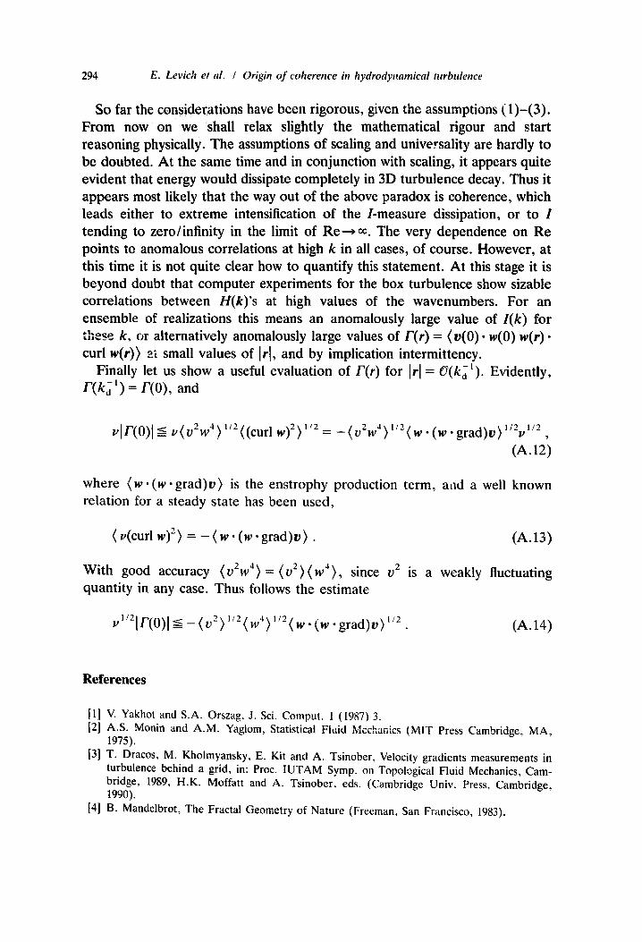
294 E. Levich et al. / Origin of coherence #1 hydrodylramical turbulence

So far the considerations have been rigorous, given the assumptions (1)-(3). From now on we shall relax slightly the mathematical rigour and start reasoning physically. The assumptions of scaling and universality are hardly to be doubted. At the same time and in conjunction with scaling, it appears quite evident that energy would dissipate completely in 3D turbulence decay. Thus it appears most likely that the way out of the above paradox is coherence, which leads either to extreme intensification of the /-measure dissipation, or to I tending to zero/infinity in the limit of Re----> 0,. The very dependence on Re points to anomalous correlations at high k in all cases, of course. However, at this time it is not quite clear how to quantify this statement. At this stage it is beyond doubt that computer experiments for the box turbulence show sizable correlations between H(k)'s at high values of the wavenumbers. For an ensemble of realizations this means an anomalously large value of l(k) for these k, or alternatively anomalously large values of F(r) = (v(O). w(O) w(r). curl w(r)) at small values of I rl, and by implication intermittency.

Finally let us show a useful evaluation of F(r) for Irl = G(kdt). Evidently, F(kS ~) = F(0), and

,,Ir(0)l _-< ~(o2w 4 ) ,,2 < (curl w)2~ 1/2 ~-- - ( u2w4~ 1/2 ( w - ( w , grad)v } 1/2v~/2,

(A.12)

where (w. (w-grad)v} is the enstrophy production term, atld a well known relation for a steady state has been used,

( v(curl w) 2 } = - ( w. (w. grad)v }. (A.13)

With good accuracy (oEw 4} = (u2}(w4}, since v 2 is a weakly fluctuating quantity in any case. Thus follows the estimate

~ 1/21V(0)l_ _ ( v2} 1,2 ( w4} ,/2 ( w. (w. grad)v }1/2 (A. 14)

References

[1] V. Yakhot and S.A. Orszag, J. Sci. Comput. 1 (1987) 3. [2] A.S. Monin and A,M. Yagiom, Statistical Fidid Mcchanics (MIT Press Cambridge, MA,

1975). [3] T. Dracos, M. Kholmyansky, E. Kit and A. Tsinober, Velocity gradients measurements in

turbulence behind a grid, in: Proc. IUTAM Symp. on Topological Fluid Mechanics, Cam- bridge, 1989, H.K. Moffatt and A. Tsinober, eds. (Cambridge Univ. Press, Cambridge, 1990).

[4] B. Mandelbrot, The Fractal Geometry of Nature (Freeman, San Francisco, 1983).


[5] A.K.M.F. Hussain, Phys. Fluids 26 (1983) 2816. [6] L Lumley, Ann. Rev. Fluid Mech. 1 (1969) 367. [7] R.H. Sellin and R.T. Moses, eds., Drag Reduction in Fluid Flows, International Association

for Hydraulic Research (Ellis Horwood, Chichester, 1989). [8] L. Lumley and I. Kubo, The influence of polymer additives on velocity and temperature

fields, in: Proc. IUTAM Symp. on Turbulent Drag Reduction, Essen, West Germany, B. Gampert, ed. (Springer, Berlin, 1985).

[9] G. Ryzkin, Phys. Rev. _ ;tt. 59 (1987) 2059. [10] H.W. Bewersdorff, Rheol. Acta 21 (1982) 587. [11] H.W. Bewersdofff, Rheol. Acta 23 (1984) 522. [12] P.G. De Gennes, Physica A 140 (1986) 9. [13] H.K. Moffatt, in: Proc. IUTAM Symp. on Turbulence and Chaotic Phenomena in Fluids,

Kyoto, Japan 1983 (North-Holland, Amsterdam, 1984). [14] H.K. Moffatt, J. Fluid Mech. 159 (1985) 359. [15] E, Levich and A. Tsinober, Phys. Lett. A 93 (1983) 293. [16] E, Levich, B. Levich and A. Tsinober, Proc. IUTAM Syrup.. Kyoto, Japan, 1983 (North-

Holland, Amsterdam, 1984). [17] E. Levich, Phys. Rep. 151 (1987) 120. [18] E. Levich and L. Shtilman, Phys. Lett. A 126 (1988) 243. [19] A.V. Tur and E. Levich, Self-organization in turbulence and generation of large scale vortices

in the atmosphere in: Proc. IUTAM Turbulence Symp. on Novel Experiments and Data Processing for Bast~ Understanding of Turbulence, Kyoto, Japan, 1990; Fluid Dyn. Res. (1991), to be published.

[20] R.B. Pelz, L. Shtilman and A. Tsinober, Phys. Fluids 29 (1986) 3506. [21] L. Shtilman, E. Levich, S.A. Orszag, R.B. Pelz and A. Tsinober, Phys. Lett. 113 (1985) 32. [22] M.M. Rogers and E Moin, Phys. Fluids 30 (1987) 2662. [23] E. Levich and L. Shtilman, fluctuating topology, generic coherence and intermittency in

turbulence, J. Fluid Mech. (1990), submitted. [24] E. Levich, Y. Murakami and L. Shtilman, Concerning one possibility of turbulence control-

ling, Phys. Left. A, submitted. [25] Y. Murakami, L. Shtilman and E. Levich, Reducing turbulence by phase juggling, Phys.

Fluids A, submitted. [26] E. Levich, Coherence versus renormalization group theory in turbulence, Phys. Rev. A,

submitted. [27] H.K. Moffatt, The topological as opposed to analytical approach to the fluid and plasma flow

problems, in: Proc. IUTAM Symp. on Topological Fluid Mechanics, Cambridge, 1989, H.K. Moffatt and A. Tsinober, eds. (Cambridge Univ. Press, Cambridge, 1990).

[28] V. Tur and V.V. Yanovsky, Invariants in dissipationless hydrodynamic media, preprint Space Research Institute, Academy of Sciences USSR.

[29] H.K. Moffatt, J. Fluid Mech. 35 (1969) 117. [30] V.I. Arnold, The asymptotic Hopf invariant and its applications, in: Proc. Summer School in

Differential Equations, Erevan, Armenian SSR Acad. Scl., 1979, E~gl. Translation in: Sol. Math. Soy. 5 (1986) 327.

[31] M.A. Berger, In: Proc. IUTAM Symp. on Topoiogicai Fluid Mechanics, Cambridge, 1989, H.K. Moffatt and A. Tsinober, eds. (Cambridge Uni~. Press, Cambridge, 1990).

[32] M.A. Berger and G.B. Field, J. Fluid Mech. 147 (1984) 133. [33] E. Levich and E. Tzvetkov, Phys. Rep. 128 (1985), 1. [34] E. Kit, E. Levich, L. Shtilman and A. Tsinober, Phys. Chem. Hyd. J. 10 (1988) 615. [35] E. Levich, Anomalous helicity fluctuations and coherence in turbulence: theory and experi-

ment, in: Proc. IUTAM Symp. on Topological Fluid Mechanics, H.K. Moffatt and A. Tsinober, eds. (Cambridge Univ. Press, Cambridge, 1990).

[36] W. Polifke, Thesis, City College of CUNY (1990). [37] E. Levich and L. Shtilman, Helicity fluctuations and coherence in developed turbulence, in:


Proc. Symp. on Scaling, Fractals and Nonlinear Variability in Geophysics I, Montreal, D. Schertzer and S, Lovejoy, eds. (Kluwer, Dordrecht, 1990).

[38] A.V. Tur, G.A. Khomenko and V.V. Yanovsky, in: Nonlinear and Turbulent Processes in Physics, vol. 2 R.Z. Sagdeev, ed. (Gordon and Breach, New York, 1984) p. 1073.

[39] S.S. Moiseev, R.Z. Sagdeev, A.V. Tur, G.A. Khomenko and V.V. Yanovsky, Soy. Phys. JETP 58 (1983) 1144.

[40] D. Forster, D. Nelson and M.G. Stephen, Phys. Rev. A 116 (1977) 172. [41] W.D. McComb, The Physics of Fluid Turbulence (Clarendon, Oxford, 1990). [42] E.V. Theodorovich, Soviet JETP 96 (1979) 163. [43] R.H. Kraichnan, Phys. Rev. A 25 (1982) 3281. [44] L, Shtilman and W. Polifke, Phys. Fluids A 1 (1989) 778. [45] W. Polifke and L. Shtilman, Phys. Fluid A 1 (1989) 2025. [46] M.J. Lee, Ph.D. Thesis, Stanford University (1985). [47] M.M. Rogers, Ph.D. Thesis, Stanford University (1988). [48] J.M. Wallace and J.-L. Balint, An experimental study of helicity and related properties in

turbulent flow, Proc. IUTAM Symp. on Topological Fluid Mechanics, H.K. Moffatt and A. Tsinober, eds. (Cambridge Univ. Press, Cambridge, 1990).

[49] E. Kit, A. Tsinober, J.L. Ballint, J.M. Wallace and E. Levich, Phys. Fluids 30 (1987) 3323. [50] G.K. Batchelor, J. Fluid Mech. 46 (1971) 813. [51] Wm.T. Ashurst, A.R. Kerstein, R.M. Kerr and G.H. Gibson, Phys. Fluids 30 (1987) 2343. [52] R.H. Kraichnan and R. Panda, Phys. Fluids 31 (1988) 2395. [53] R. Penrose, Emperors New Mind (Oxford Univ. Press, Oxford, 1989) pp. 326-347. [54] V.V. Gvaramadze, G.A. Khomenko and A.V. Tur, Geophys. Astrophys. Fluid Dyn. 17 (1988)

1. [55] R. Handler, E. Levich and L. Sirovich, Reducing turbulent drag in the channel flow by phase

randomization (1990), to be submitted. [56] O.A. Druzhinin, G.A. Khomenko and S.S. Moiseev, Turbulent Forcing and Large-Scale

Instability of Compressible Flows, Nonlinear World (World Scientific, Singapore, 1990). [57] T. Passot, A. Pouquet and P.L. Sulem, Large-scale dynamics of compressible flows, Physica

D, to appear. [58] O.A. Druzhinin and G.A. Khomenko, Nonlinear hydrodynamical alpha-effect and inverse

energy cascade in turbulence of compressible fluids, Phys. Lett. A, to appear. [59] G.A. Khomenko, S.S. Moiseev and A.V. Tur, The hydrodynam~cal alpha-effect in a com-

pressible medium, J. Fired Mech., to appear. [60] S.S. Moiseev, P.B. Rutkevich, A.V. Tur and V.V. Yanovsky, Z. Exp. Teor. Fiz. 94 (1988) 144

(Engl. transl, in Sov. Phys. JETP).

The origin of coherence in hydrodynamical turbulence

Documents