The Optimal Hard Threshold for Singular Values is 4 3 · The Optimal Hard Threshold for Singular Values is 4= p 3 Matan Gavish and David L. Donoho ... TSVD and other popular shrinkage

1

The Optimal Hard Thresholdfor Singular Values is 4/

√3

Matan Gavish and David L. Donoho

Abstract—We consider recovery of low-rank matrices fromnoisy data by hard thresholding of singular values, in whichempirical singular values below a threshold λ are set to 0. Westudy the asymptotic MSE (AMSE) in a framework where thematrix size is large compared to the rank of the matrix to berecovered, and the signal-to-noise ratio of the low-rank piecestays constant. The AMSE-optimal choice of hard threshold, inthe case of n-by-n matrix in white noise of level σ, is simply(4/√3)√nσ ≈ 2.309

√nσ when σ is known, or simply 2.858·ymed

when σ is unknown, where ymed is the median empiricalsingular value. For nonsquare m by n matrices with m 6= nthe thresholding coefficients 4/

√3 and 2.858 are replaced with

different provided constants that depend on m/n. Asymptotically,this thresholding rule adapts to unknown rank and unknownnoise level in an optimal manner: it is always better than hardthresholding at any other value, and is always better than idealTruncated SVD (TSVD), which truncates at the true rank of thelow-rank matrix we are trying to recover. Hard thresholding atthe recommended value to recover an n-by-n matrix of rankr guarantees an AMSE at most 3nrσ2. In comparison, theguarantees provided by TSVD, optimally tuned singular valuesoft thresholding and the best guarantee achievable by anyshrinkage of the data singular values are 5nrσ2, 6nrσ2, and2nrσ2, respectively. The recommended value for hard thresholdalso offers, among hard thresholds, the best possible AMSEguarantees for recovering matrices with bounded nuclear norm.Empirical evidence suggests that performance improvement overTSVD and other popular shrinkage rules can be substantial, fordifferent noise distributions, even in relatively small n.

Index Terms—Singular values shrinkage, optimal threshold,low-rank matrix denoising, unique admissible, scree plot elbowtruncation, quarter circle law, bulk edge.

I. INTRODUCTION

SUPPOSE that we are interested in an unknown m-by-nmatrix X , thought to be either exactly or approximately of

low rank, but we only observe a single noisy m-by-n matrixY , obeying Y = X+σZ. The noise matrix Z has independent,identically distributed, zero-mean entries. The matrix X is a(non-random) parameter, and we wish to estimate it with somebound on the mean squared error (MSE).

The default estimation technique for our task is TruncatedSVD (TSVD) [2]: Write

Y =

m∑i=1

yiuiv′i (1)

for the Singular Value Decomposition of the data matrix Y ,where ui ∈ Rm and vi ∈ Rn, i = 1, . . . ,m are the left and

The authors are with the Department of Statistics, Stanford University, Stan-ford, CA 94305 USA (e-mail: [email protected]; [email protected])

right singular vectors of Y corresponding to the singular valueyi. The TSVD estimator is

Xr =

r∑i=1

yiuiv′i ,

where r = rank(X), assumed known, and y1 ≥ . . . ≥ ym.Being the best approximation of rank r to the data in theleast squares sense [3], and therefore the Maximum Likelihoodestimator when Z has Gaussian entries, the TSVD is arguablyas ubiquitous in science and engineering as linear regression[4]–[9].

When the true rank r of the signal X is unknown, onemight try to form an estimate r and then apply the TSVD Xr.Extensive literature has formed on methods to estimate r: wepoint to the early [9], [10] (in Factor Analysis and PrincipalComponent Analysis), the recent [11]–[13] (in our settingof Singular Value Decomposition), and reference therein.It is instructive to think about rank estimation (using anymethod), followed by TSVD, simply as hard thresholding ofthe data singular values, where only components yiuiv′i forwhich yi passes a specified threshold, are included in X . LetηH(y, τ) = y1{y≥τ} denote the hard thresholding nonlinearity,and consider Singular Value Hard Thresholding (SVHT)

Xτ =

m∑i=1

ηH(yi; τ)uiv′i . (2)

In words, Xτ sets to 0 any data singular value below τ .Matrix denoisers explicitly or implicitly based on hard

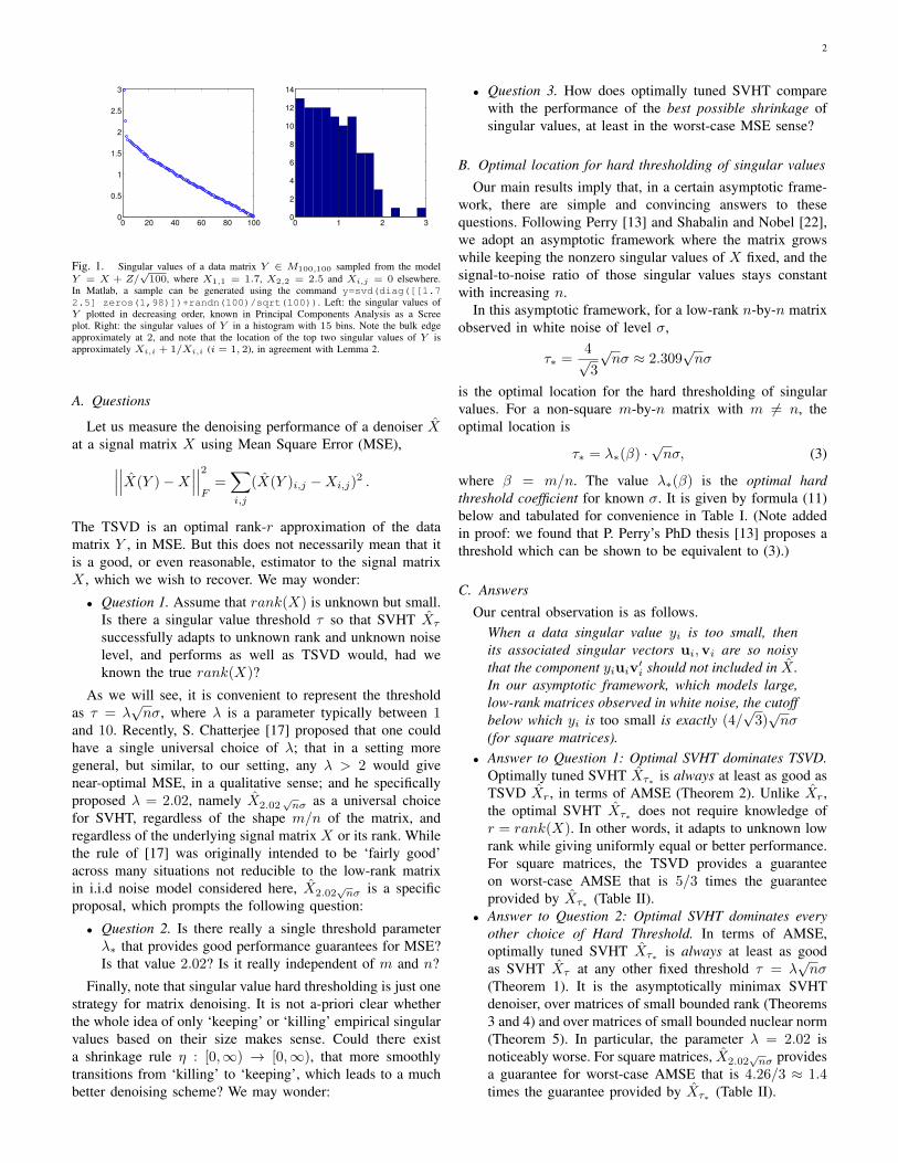
thresholding of singular values have been proposed by manyauthors, including [12]–[20]. As a common example of im-plicit SVHT denoising, consider the standard practice ofestimating r by plotting the singular values of Y in decreasingorder, and looking for a “large gap” or “elbow” (Figure 1, leftpanel). When X is exactly or approximately low-rank and theentries of Z are white noise of zero mean and unit variance,the empirical distribution of the singular values of the m-by-nmatrix Y = X + σZ forms a quarter-circle bulk whose edgelies approximately at (1 +

√β) ·√nσ, with β = m/n [21].

Only data singular values that are larger than the bulk edgeare noticeable in the empirical distribution (Figure 1, rightplot). Since the singular value plot “elbow” is located at thebulk edge, the popular method of TSVD at the “elbow” is anapproximation of bulk-edge hard thresholding, X(1+

√β)√nσ .

arX

iv:1

305.

5870

v3 [

stat

.ME

] 4

Jun

201

4

2

0 20 40 60 80 1000

0.5

1

1.5

2

2.5

3

0 1 2 30

2

4

6

8

10

12

14

Fig. 1. Singular values of a data matrix Y ∈ M100,100 sampled from the modelY = X + Z/

√100, where X1,1 = 1.7, X2,2 = 2.5 and Xi,j = 0 elsewhere.

In Matlab, a sample can be generated using the command y=svd(diag([[1.72.5] zeros(1,98)])+randn(100)/sqrt(100)). Left: the singular values ofY plotted in decreasing order, known in Principal Components Analysis as a Screeplot. Right: the singular values of Y in a histogram with 15 bins. Note the bulk edgeapproximately at 2, and note that the location of the top two singular values of Y isapproximately Xi,i + 1/Xi,i (i = 1, 2), in agreement with Lemma 2.

A. Questions

Let us measure the denoising performance of a denoiser Xat a signal matrix X using Mean Square Error (MSE),∣∣∣∣∣∣X(Y )−X

∣∣∣∣∣∣2F=∑i,j

(X(Y )i,j −Xi,j)2 .

The TSVD is an optimal rank-r approximation of the datamatrix Y , in MSE. But this does not necessarily mean that itis a good, or even reasonable, estimator to the signal matrixX , which we wish to recover. We may wonder:

• Question 1. Assume that rank(X) is unknown but small.Is there a singular value threshold τ so that SVHT Xτ

successfully adapts to unknown rank and unknown noiselevel, and performs as well as TSVD would, had weknown the true rank(X)?

As we will see, it is convenient to represent the thresholdas τ = λ

√nσ, where λ is a parameter typically between 1

and 10. Recently, S. Chatterjee [17] proposed that one couldhave a single universal choice of λ; that in a setting moregeneral, but similar, to our setting, any λ > 2 would givenear-optimal MSE, in a qualitative sense; and he specificallyproposed λ = 2.02, namely X2.02

√nσ as a universal choice

for SVHT, regardless of the shape m/n of the matrix, andregardless of the underlying signal matrix X or its rank. Whilethe rule of [17] was originally intended to be ‘fairly good’across many situations not reducible to the low-rank matrixin i.i.d noise model considered here, X2.02

√nσ is a specific

proposal, which prompts the following question:

• Question 2. Is there really a single threshold parameterλ∗ that provides good performance guarantees for MSE?Is that value 2.02? Is it really independent of m and n?

Finally, note that singular value hard thresholding is just onestrategy for matrix denoising. It is not a-priori clear whetherthe whole idea of only ‘keeping’ or ‘killing’ empirical singularvalues based on their size makes sense. Could there exista shrinkage rule η : [0,∞) → [0,∞), that more smoothlytransitions from ‘killing’ to ‘keeping’, which leads to a muchbetter denoising scheme? We may wonder:

• Question 3. How does optimally tuned SVHT comparewith the performance of the best possible shrinkage ofsingular values, at least in the worst-case MSE sense?

B. Optimal location for hard thresholding of singular values

Our main results imply that, in a certain asymptotic frame-work, there are simple and convincing answers to thesequestions. Following Perry [13] and Shabalin and Nobel [22],we adopt an asymptotic framework where the matrix growswhile keeping the nonzero singular values of X fixed, and thesignal-to-noise ratio of those singular values stays constantwith increasing n.

In this asymptotic framework, for a low-rank n-by-n matrixobserved in white noise of level σ,

τ∗ =4√3

√nσ ≈ 2.309

√nσ

is the optimal location for the hard thresholding of singularvalues. For a non-square m-by-n matrix with m 6= n, theoptimal location is

τ∗ = λ∗(β) ·√nσ, (3)

where β = m/n. The value λ∗(β) is the optimal hardthreshold coefficient for known σ. It is given by formula (11)below and tabulated for convenience in Table I. (Note addedin proof: we found that P. Perry’s PhD thesis [13] proposes athreshold which can be shown to be equivalent to (3).)

C. Answers

Our central observation is as follows.When a data singular value yi is too small, thenits associated singular vectors ui,vi are so noisythat the component yiuiv′i should not included in X .In our asymptotic framework, which models large,low-rank matrices observed in white noise, the cutoffbelow which yi is too small is exactly (4/

√3)√nσ

(for square matrices).• Answer to Question 1: Optimal SVHT dominates TSVD.

Optimally tuned SVHT Xτ∗ is always at least as good asTSVD Xr, in terms of AMSE (Theorem 2). Unlike Xr,the optimal SVHT Xτ∗ does not require knowledge ofr = rank(X). In other words, it adapts to unknown lowrank while giving uniformly equal or better performance.For square matrices, the TSVD provides a guaranteeon worst-case AMSE that is 5/3 times the guaranteeprovided by Xτ∗ (Table II).

• Answer to Question 2: Optimal SVHT dominates everyother choice of Hard Threshold. In terms of AMSE,optimally tuned SVHT Xτ∗ is always at least as goodas SVHT Xτ at any other fixed threshold τ = λ

√nσ

(Theorem 1). It is the asymptotically minimax SVHTdenoiser, over matrices of small bounded rank (Theorems3 and 4) and over matrices of small bounded nuclear norm(Theorem 5). In particular, the parameter λ = 2.02 isnoticeably worse. For square matrices, X2.02

√nσ provides

a guarantee for worst-case AMSE that is 4.26/3 ≈ 1.4times the guarantee provided by Xτ∗ (Table II).

3

• Answer to Question 3. Optimal SVHT compares ade-quately to the optimal shrinker. Optimally tuned SVHTXτ∗ provides a guarantee on worst-case asymptotic MSEthat is 3/2 times (for square matrices) the best possibleguarantee achievable by any shrinkage of data singularvalues (Table II).

These are all rigorous results, within a specific asymptoticframework, which prescribes a certain scaling of the noiselevel, the matrix size, and the signal-to-noise ratio as n grows.But does AMSE predict actual MSE in finite-sized problems?In Section VII we show finite-n simulations demonstratingthe effectiveness of these results even at rather small problemsizes. In high signal-to-noise, all denoisers considered hereperform roughly the same, and in particular the classicalTSVD is a valid choice in that regime. However, in lowand moderate SNR, the performance gain of optimally tunedSVHT is substantial, and can offer 30% − 80% decrease inAMSE.

D. Optimal singular value hard thresholding – In practice

For a low-rank n-by-n matrix observed in white noise ofunknown level, one can use the data to obtain an approximationof the optimal location τ∗. Define

τ∗ ≈ 2.858 · ymed ,

where ymed is the median singular value of the data matrixY . The notation τ∗ is meant to emphasize that this is not afixed threshold chosen a-priori, but rather a data-dependentthreshold. For a non-square m-by-n matrix with m 6= n, theapproximate optimal location when σ is unknown is

τ∗ = ω(β) · ymed . (4)

The optimal hard threshold coefficient for unknown σ, denotedby ω(β), is not available as an analytic formula, but can easilybe evaluated numerically. We provide a Matlab script for thispurpose [1]; the underlying derivation appears in Section III-Ebelow. Some values of ω(β) are provided in Table IV. Whena high-precision value of ω(β) cannot be computed, one canuse the approximation

ω(β) ≈ 0.56β3 − 0.95β2 + 1.82β + 1.43 . (5)

The optimal SVHT for unknown noise level, Xτ∗ , is very sim-ple to implement and does not require any tuning parameters.The denoised matrix Xτ∗(Y ) can be computed using just a fewcode lines in a high-level scripting language. For example, inMatlab:

beta = size(Y,1) / size(Y,2);omega = 0.56*betaˆ3 - 0.95*betaˆ2 + ...

1.82*beta + 1.43;[U D V] = svd(Y);y = diag(Y);y( y < (omega * median(y) ) = 0;Xhat = U * diag(y) * V’;

Here we have used the approximation (5). We recommend,whenever possible, to use a function omega(beta), such as

the one we provide in the code supplement [1], to computethe coefficient ω(β) to high precision.

In our asymptotic framework, τ∗ and τ∗ enjoy exactly thesame optimality properties. This means that Xτ∗ adapts tounknown low rank and to unknown noise level. Empiricalevidence suggest that their performance for finite n is similar.As a result, the answers we provide above hold for thethreshold τ∗ when the noise level is unknown, just as theyhold for the threshold τ∗ when the noise level is known.

II. PRELIMINARIES AND SETTING

Column vectors are denoted by boldface lowercase letters,such as v, their transpose is v′ and their i-th coordinate is vi.The Euclidean inner product and norm on vectors are denotedby 〈u , v〉 and ||u||2, respectively. Matrices are denotes byuppercase letters, such as X , its transpose is X ′ and theiri, j-th entry is Ai,j . Mm×n denotes the space of real m-by-n matrices, 〈X , Y 〉 =

∑i,j Xi,jYi,j denotes the Hilbert-

Schmidt inner product, and ||X||F denotes the correspondingFrobenius norm on Mm×n. For simplicity we only considerm ≤ n. We denote matrix denoisers, or estimators, by X :Mm×n → Mm×n. The symbols a.s.−→ and a.s.

= denote almostsure convergence and equality of a.s. limits, respectively.

A. Scaling considerations in singular value thresholding

With the exception of TSVD, when σ is known, all thedenoisers we discuss operate by shrinkage of data singularvalues, namely are of the form

X :

m∑i=1

yiuiv′i 7→

m∑i=1

η(yi;λ)uiv′i (6)

where Y is given by (1) and η : [0,∞) → [0,∞) is someunivariate shrinkage rule. As we will see, in the general modelY = X + σZ, the noise level in the singular values of Yis√nσ. Instead of specifying a different shrinkage rule that

depends on the matrix size n, we calibrate our shrinkage rulesto the “natural” model Y = X + Z/

√n. In this convention,

shrinkage rules stay the same for every value of n, and weconveniently abuse notation by writing X as in (6) for anyX : Mm×n → Mm×n, keeping m and n implicit. To applyany denoiser X below to data from the general model Y =X + σZ, use the denoiser

X(n,σ)(Y ) =√nσ · X(Y/

√nσ) . (7)

For example, to apply the SVHT

Xλ :

m∑i=1

yiuiv′i 7→

m∑i=1

ηH(yi;λ)uiv′i

to data sampled from the model Y = X + σZ, use Xτ , with

τ = λ ·√nσ .

Throughout the text, we use Xλ to denote SVHT calibratedfor noise level 1/

√n and Xτ to denote SVHT calibrated for

a specific general model Y = X + σZ.

4

To translate the AMSE of any denoiser X , calibrated fornoise level 1/

√n, to an approximate MSE of the correspond-

ing denoiser X(n,σ), calibrated for a model Y = X +σZ, weuse the identity∣∣∣∣∣∣X(n,σ)(Y )−X

∣∣∣∣∣∣2F=

n · σ2 ·∣∣∣∣∣∣X(X/(

√nσ)) + Z/

√n)−X/(

√nσ)

∣∣∣∣∣∣2F.

Below, we spell out this translation of AMSE where appro-priate.

B. Asymptotic framework and problem statement

In this paper, we consider a sequence of increasingly largerdenoising problems Yn = Xn + Zn/

√n, with Xn, Zn ∈

Mmn,n, satisfying the following assumptions:

1) Invariant white noise: The entries of Zn are i.i.d samplesfrom a distribution with zero mean, unit variance andfinite fourth moment. To simplify the formal state-ment of our results, we assume that this distributionis orthogonally invariant in the sense that Zn followsthe same distribution as AZnB, for every orthogonalA ∈ Mmn,mn and B ∈ Mn,n. This is the case,for example, when the entries of Zn are Gaussian. InSection VI we revisit this restriction and discuss general(not necessarily invariant) white noise.

2) Fixed signal column span (x1, . . . , xr): Let the rank r >0 be fixed and choose a vector x ∈ Rr with coordinatesx = (x1, . . . , xr) such that x1 ≥ . . . ≥ xr > 0. Assumethat for all n,

Xn = Un diag(x1, . . . , xr, 0, . . . , 0)V′n (8)

is an arbitrary1 singular value decomposition of Xn,where Un ∈Mmn,mn and Vn ∈Mn,n.

3) Asymptotic aspect ratio β: The sequence mn is suchthat mn/n → β. To simplify our formulas, we assumethat 0 < β ≤ 1.

Let X be any singular value shrinkage denoiser calibrated,as discussed above, for noise level 1/

√n. Define the Asymp-

totic MSE (AMSE) of an X at a signal x by the (almost sure)limit2

M(X,x)a.s.= lim

n→∞

∣∣∣∣∣∣X(Yn)−Xn

∣∣∣∣∣∣2F. (9)

Adopting the asymptotic framework above, we seek sin-gular value thresholding rules Xλ that minimize the AMSEM(Xλ,x). As we will see, in this framework there are simple,satisfying answers to the questions posed in the introduction.

1While the signal rank r and nonzero signal singular values x1, . . . , xrare shared by all matrices Xn, the signal left and right singular vectors Unand Vn are unknown and arbitrary.

2Our results imply that the AMSE is well-defined as a function of the signalsingular values x.

β λ∗(β) β λ∗(β)

0.05 1.5066 0.55 2.01670.10 1.5816 0.60 2.05330.15 1.6466 0.65 2.08870.20 1.7048 0.70 2.12290.25 1.7580 0.75 2.15610.30 1.8074 0.80 2.18830.35 1.8537 0.85 2.21970.40 1.8974 0.90 2.25030.45 1.9389 0.95 2.28020.50 1.9786 1.00 2.3094

TABLE ISOME OPTIMAL HARD THRESHOLD COEFFICIENTS λ∗(β) FROM (3). FOR m-BY-n

MATRIX IN KNOWN NOISE LEVEL σ (WITH m/n = β), THE OPTIMAL SVHTDENOISER Xτ∗ SETS TO ZERO ALL DATA SINGULAR VALUES BELOW THE

THRESHOLD τ∗ = λ∗(β)√nσ.

III. RESULTS

Define the optimal hard threshold for singular values forn-by-n square matrices by

λ∗ =4√3. (10)

More generally, define the optimal threshold for m-by-nmatrices with m/n = β by

λ∗(β)def=

√2(β + 1) +

8β

(β + 1) +√β2 + 14β + 1

. (11)

Some values of λ∗(β) are provided in Table I.

A. Optimally tuned SVHT asymptotically dominates TSVD andany SVHT

Our primary result is simply that Xλ∗ always has equal orbetter AMSE compared to SVHT with any other choice ofthreshold, and compared to TSVD. In other words, from theideal perspective of our asymptotic framework, the decision-theoretic picture is very straightforward: TSVD is asymptoti-cally inadmissible, and so is any SVHT with λ 6= λ∗. We notethat since AMSE of SVHT with λ < 1+

√β in our framework

turns out to be infinite, here and below we need only considerSVHT with λ > 1+

√β. As discussed in Section VIII, AMSE

calculation in the case where the threshold λ is placed exactlyat the bulk edge 1+

√β is a little more subtle and lies beyond

our current scope.

Theorem 1. The threshold λ∗ is asymptotically optimal forSVHT. Let 0 < β ≤ 1. For any λ > 1+

√β, any r ∈ N and

any x ∈ Rr, the AMSE (9) of the SVHT denoiser Xλ is welldefined and

M(Xλ∗ ,x) ≤M(Xλ,x) , (12)

where λ∗ = λ∗(β) is the optimal threshold (11). Moreover,if λ 6= λ∗(β), strict inequality holds at least at one pointx∗(λ) ∈ Rr.

We can therefore say that λ∗(β) is asymptotically uniqueadmissible for SVHT. In particular, the popular practice ofhard thresholding close to the bulk edge is asymptotically in-admissible. The popular Truncated SVD Xr is asymptoticallyinadmissible, too:

5

Theorem 2. Asymptotic inadmissibility of TSVD. Let 0 <β ≤ 1. For any r ∈ N and any x ∈ Rr, the AMSE of theTSVD estimator Xr is well defined, and

M(Xλ∗ ,x) ≤M(Xr,x) . (13)

Moreover, strict inequality holds at least at one point x∗(λ) ∈Rr.

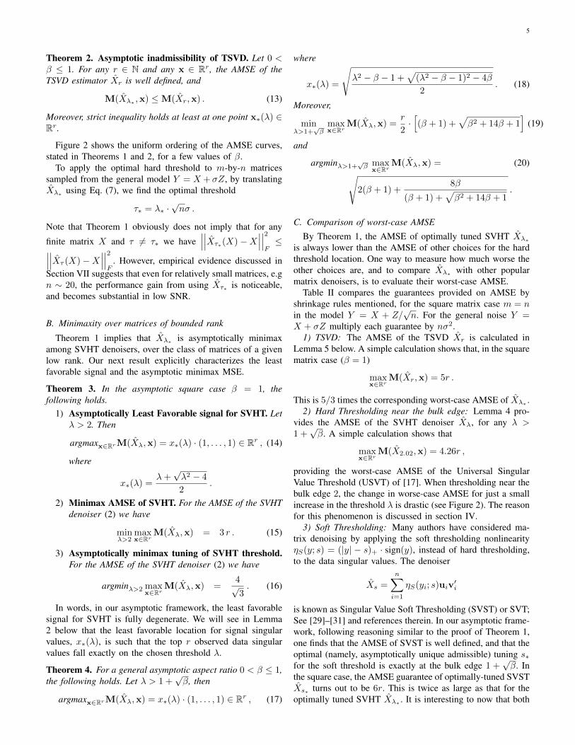
Figure 2 shows the uniform ordering of the AMSE curves,stated in Theorems 1 and 2, for a few values of β.

To apply the optimal hard threshold to m-by-n matricessampled from the general model Y = X + σZ, by translatingXλ∗ using Eq. (7), we find the optimal threshold

τ∗ = λ∗ ·√nσ .

Note that Theorem 1 obviously does not imply that for any

finite matrix X and τ 6= τ∗ we have∣∣∣∣∣∣Xτ∗(X)−X

∣∣∣∣∣∣2F≤∣∣∣∣∣∣Xτ (X)−X

∣∣∣∣∣∣2F

. However, empirical evidence discussed inSection VII suggests that even for relatively small matrices, e.gn ∼ 20, the performance gain from using Xτ∗ is noticeable,and becomes substantial in low SNR.

B. Minimaxity over matrices of bounded rank

Theorem 1 implies that Xλ∗ is asymptotically minimaxamong SVHT denoisers, over the class of matrices of a givenlow rank. Our next result explicitly characterizes the leastfavorable signal and the asymptotic minimax MSE.

Theorem 3. In the asymptotic square case β = 1, thefollowing holds.

1) Asymptotically Least Favorable signal for SVHT. Letλ > 2. Then

argmaxx∈RrM(Xλ,x) = x∗(λ) · (1, . . . , 1) ∈ Rr , (14)

where

x∗(λ) =λ+√λ2 − 4

2.

2) Minimax AMSE of SVHT. For the AMSE of the SVHTdenoiser (2) we have

minλ>2

maxx∈Rr

M(Xλ,x) = 3 r . (15)

3) Asymptotically minimax tuning of SVHT threshold.For the AMSE of the SVHT denoiser (2) we have

argminλ>2 maxx∈Rr

M(Xλ,x) =4√3. (16)

In words, in our asymptotic framework, the least favorablesignal for SVHT is fully degenerate. We will see in Lemma2 below that the least favorable location for signal singularvalues, x∗(λ), is such that the top r observed data singularvalues fall exactly on the chosen threshold λ.

Theorem 4. For a general asymptotic aspect ratio 0 < β ≤ 1,the following holds. Let λ > 1 +

√β, then

argmaxx∈RrM(Xλ,x) = x∗(λ) · (1, . . . , 1) ∈ Rr , (17)

where

x∗(λ) =

√λ2 − β − 1 +

√(λ2 − β − 1)2 − 4β

2. (18)

Moreover,

minλ>1+

√βmaxx∈Rr

M(Xλ,x) =r

2·[(β + 1) +

√β2 + 14β + 1

](19)

and

argminλ>1+√β max

x∈RrM(Xλ,x) = (20)√

2(β + 1) +8β

(β + 1) +√β2 + 14β + 1

.

C. Comparison of worst-case AMSE

By Theorem 1, the AMSE of optimally tuned SVHT Xλ∗

is always lower than the AMSE of other choices for the hardthreshold location. One way to measure how much worse theother choices are, and to compare Xλ∗ with other popularmatrix denoisers, is to evaluate their worst-case AMSE.

Table II compares the guarantees provided on AMSE byshrinkage rules mentioned, for the square matrix case m = nin the model Y = X + Z/

√n. For the general noise Y =

X + σZ multiply each guarantee by nσ2.1) TSVD: The AMSE of the TSVD Xr is calculated in

Lemma 5 below. A simple calculation shows that, in the squarematrix case (β = 1)

maxx∈Rr

M(Xr,x) = 5r .

This is 5/3 times the corresponding worst-case AMSE of Xλ∗ .2) Hard Thresholding near the bulk edge: Lemma 4 pro-

vides the AMSE of the SVHT denoiser Xλ, for any λ >1 +√β. A simple calculation shows that

maxx∈Rr

M(X2.02,x) = 4.26r ,

providing the worst-case AMSE of the Universal SingularValue Threshold (USVT) of [17]. When thresholding near thebulk edge 2, the change in worse-case AMSE for just a smallincrease in the threshold λ is drastic (see Figure 2). The reasonfor this phenomenon is discussed in section IV.

3) Soft Thresholding: Many authors have considered ma-trix denoising by applying the soft thresholding nonlinearityηS(y; s) = (|y| − s)+ · sign(y), instead of hard thresholding,to the data singular values. The denoiser

Xs =

n∑i=1

ηS(yi; s)uiv′i

is known as Singular Value Soft Thresholding (SVST) or SVT;See [29]–[31] and references therein. In our asymptotic frame-work, following reasoning similar to the proof of Theorem 1,one finds that the AMSE of SVST is well defined, and that theoptimal (namely, asymptotically unique admissible) tuning s∗for the soft threshold is exactly at the bulk edge 1 +

√β. In

the square case, the AMSE guarantee of optimally-tuned SVSTXs∗ turns out to be 6r. This is twice as large as that for theoptimally tuned SVHT Xλ∗ . It is interesting to now that both

6

0 0.5 1 1.5 2 2.50

0.5

1

1.5

2

2.5

3

3.5

4

4.5

5

x

AM

SE

β = 0.1

X r

X 2 .02

Xλ ∗

X1+

√

β

X op t

0 0.5 1 1.5 2 2.50

0.5

1

1.5

2

2.5

3

3.5

4

4.5

5

xAM

SE

β = 0.3

0 0.5 1 1.5 2 2.50

0.5

1

1.5

2

2.5

3

3.5

4

4.5

5

x

AM

SE

β = 0.7

0 0.5 1 1.5 2 2.50

0.5

1

1.5

2

2.5

3

3.5

4

4.5

5

x

AM

SE

β = 1

Fig. 2. AMSE against signal amplitude x for denoisers discussed: TSVD Xr , universal hard threshold X2.02 from [17], and optimally tuned SVHT proposed here Xλ∗ . Alsoshown: the limiting AMSE of Xλ as λ → 1 +

√β (denoted X1+

√β ), and optimal singular value shrinkage Xopt from [28]. Different aspect ratios β are shown; r = 1

everywhere; curves jittered in vertical axis to avoid overlap.

optimal tuning for the soft threshold λ and the correspondingbest-possible AMSE guarantee agree with calculations donein an altogether different asymptotic model, in which onefirst takes n → ∞ with rank r/n → ρ, and only then takesρ→ 0 [31, sec. 8]. We also note that the worst-case AMSE ofSVST is obtained in the limit of very high SNR, where SVHTdoes very well in comparison. When both are optimally tuned,SVHT does not dominate SVST across all matrices; In fact,soft thresholding does better than hard thresholding in lowSNR (Figure 3). For example, in the square case, when thesignal is near

√3 (the least favorable location for Xλ∗ ), the

AMSE of Xs∗ is (7− 8/√3)r ≈ 2.38r, compared to 3r, the

worse-case AMSE of Xλ∗ .4) Optimal Singular Value Shrinker: Our focus in this pa-

per is denoising by singular value hard thresholding (SVHT),where Xλ acts applying a hard thresholding nonlinearity toeach of the data singular values. As mentioned in the intro-duction, one may ask how SVHT compares to other singularvalue shrinkage denoisers, which use a different nonlinearitythat may be more suitable to the problem at hand. In aspecial case of our asymptotic framework, Perry [13] andShabalin and Nobel [22] have derived an optimal singularvalue shrinker Xopt. Proceeding along this line, in [28] weexplore optimal shrinkage of singular values under variousloss functions and develop a simple expression for the optimalshrinkers. Calibrated for the model X +Z/

√n, in the square

setting m = n, this shrinker takes the form

Xopt :

n∑i=1

yiuiv′i 7→

n∑i=1

ηopt(yi)uiv′i

where

ηopt(x) =√(x2 − 4)+ .

In our asymptotic framework, this rule dominates in AMSEessentially any other estimator based on singular value shrink-age, at any configuration of the non-zero signal singular valuesx. The AMSE of the optimal shrinker (in the square matrixcase) at x ∈ Rr is [28]

M(Xopt,x) =

r∑i=1

{2− 1

x2i

xi ≥ 1

x2i 0 ≤ xi ≤ 1. (21)

(See Figure 2.) It follows that the worst-case AMSE of Xopt

ismaxx∈Rr

M(Xopt,x) = 2r

in the square case. We conclude that, for square matrices,in worst-case AMSE, singular value hard thresholding at theoptimal location is 50% worse than the best possible singularvalue shrinker, Truncated SVD or SVHT just above the bulk-edge (which roughly equals the widely used Scree-plot elbowtruncation) is 250% worse, and singular value soft thresholdingis 300% worse.

D. Minimaxity over matrices of bounded nuclear norm

So far we have considered minimaxity over the class ofmatrices of at most rank r, where r is given. In [17], theauthor considered minimax estimation over a different classof matrices, namely nuclear norm balls. For a given constantξ, this is the class of all matrices for which the nuclear normis at most ξ. Recall that the nuclear norm of a matrix X ∈Mm×n, whose vector of singular values is x ∈ Rm, is givenby ||x||1. Our next result shows that Xλ∗ is minimax optimalover this class as well. Specifically, it is the minimax estimator,in AMSE, among all SVHT rules, over a given Nuclear Normball. We note that unlike Theorems 3 and 4, this result does notfollow directly from Theorem 1. We restrict our discussion tosquare matrices (β = 1); the general nonsquare case is handledsimilarly.

Theorem 5. Let λ > 2 and let ξ = r · (λ +√λ2 − 4)/2 for

some r ∈ N.1) The least favorable singular value configuration obeys

argmax||x||1≤ξM(Xλ,x) = x∗(λ) · (1, . . . , 1) ∈ Rr , (22)

where

x∗(λ) =λ+√λ2 − 4

2.

2) The best achievable inequality between nuclear norm ξand AMSE of a hard threshold rule is:

minλ>2

max||x||1≤ξ

M(Xλ,x) =√3 · ξ . (23)

7

Shrinker Standing notation Guarantee on AMSEOptimal singular value shrinker Xopt 2r

Optimally tuned SVHT Xλ∗ 3r

Universal Singular Value Threshold [17] X2.02 ≈ 4.26r

TSVD Xr 5r

Optimally tuned SVST Xs∗ 6r

TABLE IIA COMPARISON OF GUARANTEES ON AMSE PROVIDED BY SINGULAR VALUE SHRINKAGE RULES DISCUSSED, FOR THE SQUARE MATRIX CASE m = n IN THE MODEL

Y = X + Z/√n. FOR THE GENERAL MODEL Y = X + σZ MULTIPLY EACH GUARANTEE BY nσ2 .

0 0.5 1 1.5 2 2.5 30

0.5

1

1.5

2

2.5

3

3.5

4

x

AM

SE

Xλ∗

Xs∗

Xoptimal

Fig. 3. AMSE of optimally tuned SVHT (red), optimally tuned SVST (blue) andthe optimal singular value shrinker [28] (green), for square case (β = 1) and r = 1.The best available constant from Table III is the slope of the convex envelope (dashed)of the AMSE curve (solid), namely, the slope of the secant running from the origin tothe inflection point of the AMSE curve. Although the maximum (worst-case AMSE)of optimally tuned SVST Xs∗ is higher than that of optimally tuned SVHT Xλ∗ , theslope of its convex envelope is lower.

3) The threshold achieving this inequality is

argminλ>2 max||x||1≤ξ

M(Xλ,x) =4√3. (24)

As an alternative to comparing denoisers by comparingtheir guarantees on AMSE over a prescribed rank r, one cancompare denoisers based on the best available constant C inthe inequality

minλ>2

max||x||1≤ξ

M(Xλ,x) = C · ξ . (25)

The results in the square matrix case are summarized in TableIII. Each constant is derived from the AMSE formula for therespective denoiser, as cited above. To understand why the bestavailable constant for optimally tuned SVST is smaller thanthan of optimally tuned SVHT, consider Figure 3.

E. When the noise level σ is unknown

When the noise level in which Y is observed is unknown,it no longer makes sense to use Xλ∗ , which is calibrated for aspecific noise level. We now describe a method to estimate theoptimal hard threshold from the data matrix Y . To emphasizethat the resulting denoiser is ready for use on data fromthe general model Y = X + σZ, we denote this estimatedthreshold by τ∗, and the SVHT denoiser by Xτ∗ . To this end,

we are required to estimate the unknown noise level σ. In theclosely related Spiked Covariance Model, there are existingmethods for estimation of an unknown noise level; see forexample [32] and references therein.

Consider the following robust estimator for the parameterσ in the model Y = X + σZ:

σ(Y )def=

ymed√n · µβ

, (26)

where ymed is a median singular value of Y and µβ is themedian of the the Marcenko-Pastur distribution, namely, theunique solution in β− ≤ x ≤ β+ to the equation

x∫β−

√(β+ − t)(t− β−)

2πtdt =

1

2,

where β± = (1±√β)2. Define the optimal hard threshold for

a data matrix Y ∈ Mm×n observed in unknown noise level,with m/n = β, by plugging in σ(Y ) instead of σ in Eq. (3):

τ∗(β, Y )def= λ∗(β) ·

√n σ(Y ) =

λ∗(β)√µβ

ymed .

Writing ω(β) = λ∗(β)/√µβ , the threshold is

τ∗(β, Y ) = ω(β) · ymed .

The median µβ and hence the coefficient ω(β) are notavailable analytically; in [1] we make available a Matlab scriptto evaluate the coefficient ω(β). Some values are tabulated inTable IV for convenience. A useful approximation to ω isgiven as a cubic polynomial in Eq. (5) above. Empirically,

max0.001<β≤1

|ω(β)−(0.56β3 − 0.95β2 + 1.82β + 1.43

)| ≤ 0.02

which may be sufficient for some practical purposes if onedoes not have access to a more exact value of ω.

Lemma 1. For the sequence Yn in our asymptotic framework,

limn→∞

σ(Yn)

1/√n

a.s.= 1.

Correlary 1. For Yn as above and any 0 < β ≤ 1,

limn→∞

τ∗(β, Yn)a.s.= λ∗(β) · lim

n→∞

√n · σ(Yn)

a.s.= λ∗(β) ,

Correlary 2. For Yn as above, any 0 < β ≤ 1, any r and anyx ∈ Rr, almost surely

M(Xτ∗ ,x) = M(Xλ∗ ,x) .

Correlary 3. Theorem 1, Theorem 2, Theorem 3, Theorem4 and Theorem 5 all hold if we replace the optimally-tuned

8

TABLE IIIA COMPARISON OF BEST AVAILABLE CONSTANT IN MINIMAX AMSE, OVER NUCLEAR NORM BALLS, FOR THE SHRINKAGE RULES DISCUSSED, FOR THE SQUARE MATRIX CASE

m = n IN THE MODEL Y = X + Z/√n. THESE CONSTANTS ARE THE SAME FOR THE GENERAL MODEL Y = X + σZ .

Shrinker Standing notation Best possible constant C in Eq. (25)Optimal singular value shrinker Xopt 1

Optimally tuned SVHT Xλ∗√3 ≈ 1.73

USVT of [17] X2.02 ≈ 3.70

TSVD Xr 5

Optimally tuned SVST Xs∗ ≈ 1.38

β ω(β) β ω(β)

0.05 1.5194 0.55 2.23650.10 1.6089 0.60 2.30210.15 1.6896 0.65 2.36790.20 1.7650 0.70 2.43390.25 1.8371 0.75 2.50110.30 1.9061 0.80 2.56970.35 1.9741 0.85 2.63990.40 2.0403 0.90 2.70990.45 2.106 0.95 2.78320.50 2.1711 1.00 2.8582

TABLE IVSOME VALUES OF THE OPTIMAL HARD THRESHOLD COEFFICIENT FOR UNKNOWN

NOISE LEVEL, ω(β) OF EQ. (4) FOR AN m-BY-n MATRIX IN UNKNOWN NOISE LEVEL

(WITH m/n = β), THE OPTIMAL SVHT DENOISER Xτ∗ SETS TO ZERO ALL DATA

SINGULAR VALUES BELOW THE THRESHOLD τ∗ = ω(β)ymed , WHERE ymed IS THE

MEDIAN SINGULAR VALUE OF THE DATA MATRIX Y . CALCULATED USING FUNCTION

PROVIDED IN THE CODE SUPPLEMENT [1].

SVHT for known σ, Xλ∗(β), by optimally-tuned SVHT forunknown σ, Xτ∗ .

IV. DISCUSSION

A. The optimal threshold λ∗(β) and the bulk edge 1 +√β

Figure 4 shows the optimal threshold λ∗(β) over β. Theedge of the quarter circle bulk 1+

√β, the hard threshold that

best emulates TSVD in our setting, is shown for comparison.In the null case X = 0, the largest data singular value islocated asymptotically exactly at the bulk edge, 1 +

√β. It

might seem that just above the bulk edge is a natural place toset a threshold, since anything smaller could be the productof a pure noise situation. However, for β > 0.2, the optimalhard threshold λ∗(β) is 15-20% larger than the bulk edge;as β → 0, it grows about 40% larger. Inspecting the proof ofTheorem 1 and particularly the expression for AMSE of SVHT(Lemma 4), one finds the reason: one component of the AMSEis due to the angle between the signal singular vectors andthe data singular vectors. This angle converges to a nonzerovalue as n→∞ (given explicitly in Lemma 3) which growsas SNR decreases. When some data singular value yi is tooclose to the bulk, its corresponding singular vectors are toobadly rotated, and the rank-one matrix yiuiv′i it contributes tothe denoiser hurts the AMSE more than it helps. For example,for square matrices β = 1, this situation is most acute whenthe signal singular value is just barely larger than xi = 1,causing the corresponding data singular value yi to be justbarely larger than the bulk edge, which for square matricesis located at 2. A SVHT denoiser thresholding just abovethe bulk edge would include the component yiuiv′i, incurring

0 0.2 0.4 0.6 0.8 11

1.5

2

2.5

β

λ

λ∗(β)

1 +√

β

2.02

Fig. 4. The optimal threshold λ∗(β) from (11) against β. Also shown are bulk-edge1 +√β, which is the hard threshold corresponding to TSVD in our setting, and the

USVT threshold 2.02 from [17].

an AMSE about 5 times larger than the AMSE incurred byexcluding yi from the reconstruction. The optimal thresholdλ∗(β) keeps such singular values out of the picture; this is whyit is necessarily larger than the bulk edge. The precise value ofλ∗(β) is the precise point at which it becomes advantageousto include the rank-one contribution of a singular value yi inthe reconstruction.

B. The optimal threshold λ∗(β) relative to the USVT X2.02

As mentioned in the introduction, S. Chatterjee has recentlydiscussed SVHT in a broad class of situations [17]. Translatinghis much broader discussion to the confines of the presentcontext, he observed that any λ > 2 can serve as a universalhard threshold for singular values (USVT), offering fairlygood performance regardless of the matrix shape m/n andthe underlying signal matrix X . The author makes the specificrecommendation λ = 2.02 and writes:

“The algorithm manages to cut off the singular val-ues at the ‘correct’ level, depending on the structureof the unknown parameter matrix. The adaptivenessof the USVT threshold is somewhat similar in spiritto that of the SureShrink algorithm of Donoho andJohnstone.“

Keeping in mind that the scope of [17] is much broaderthan the one considered here, we would like to evaluatethis proposal, in the setting of low rank matrix in whitenoise, and specifically in our asymptotic framework. Figure

9

0 0.2 0.4 0.6 0.8 11

1.5

2

2.5

3

3.5

4

4.5

β

AMSE

maxx M(X2.02, x)

maxx M(Xλ∗(β ), x)

Fig. 5. Worst-case AMSE against the shape parameter β, for two choices of hardthreshold: λ = 2.02 from [17], and optimal threshold λ∗ from (11).

4 includes the value 2.02: indeed, this threshold is largerthan the bulk edge, for any 0 < β ≤ 1, so Chatterjee’sX2.02 rule asymptotically set to zero all singular values whichcould arise due to an underlying noise-only situation. Whenλ∗(β) < 2.02, the X2.02 rule sometimes “kills” singular valuesthat the optimal threshold deems good enough for keeping,and when λ∗(β) > 2.02, the X2.02 rule sometimes “keeps”singular values that did in fact arise from signal, but are soclose to the bulk that the optimal threshold declares themunusable.

For β = 1, the guarantee on worst-case AMSE obtainedby using λ = 2.02 over matrices of rank r is about 4.26r,roughly 140% larger than the guarantee obtained by usingthe minimax threshold λ = 4/

√3 (See Figure 2). For square

matrices, the regret for preferring USVT to optimally-tunedSVHT can be substantial: in low SNR (x ≈ 1), using thethreshold λ = 2.02 incurs roughly twice the AMSE of theminimax threshold 4/

√3.

We note that unlike the optimally tuned SVHT Xλ∗ , theUSVT X2.02 does not take into account the shape factor β,namely the ratio of number of rows to number of columnsof the matrix in question. A comparison of worst-case AMSEbetween the fixed threshold choice λ = 2.02 and the optimalhard threshold λ = λ∗(β) is shown in Figure 5. The twocurves intersect at λ ≈ 0.55, where the optimal threshold (11)is approximately 2.02.

One might argue that [17] proposed 2.02 based on its MSEperformance over classes of matrices bounded in nuclear norm.But also for that purpose, 2.02 is noticeably outperformed byλ∗(β). Arguing as in Theorem 5 we obtain, in the square case:

max||x||1≤ξ

M(X2.02,x) ≈ 3.70 · ξ . (27)

The coefficient 3.70 is about 110% larger than the bestcoefficient achievable by SVHT, namely C =

√3 in (25).

One should keep in mind that USVT is applicable for a widerange of noise models, e.g. in stochastic block models. [17] isthe first, to the best of out knowledge, to suggest that a matrixdenoising procedure as simple as SVHT could have universaloptimality properties. In our asymptotic framework of low-rank matrices in white noise, the 2.02 threshold performs fairlywell in AMSE, except for very small values of β (Figure

2); but one often gets a substantial AMSE improvement byswitching to the rule we recommend. Since our recommenda-tion dominates in AMSE, there is no downside to making thisswitch – i.e. there is no configuration of signal singular valuesx which could make one regret this switch.

V. PROOFS

Setting additional notation required in the proofs, let

Xn =

r∑i=1

xi an,i b′n,i

be a sequence of signal matrices in our asymptotic framework,so that an,i ∈ Rmn (resp. bn,i ∈ Rn) is the left (resp.right) singular vector corresponding to the singular value xi,namely, i-th column of Un (resp. Vn) in (39). Similarly, letYn be a corresponding sequence of observed matrices in ourframework, and write

Yn =

mn∑i=1

yn,i un,i v′n,i

so that un,i ∈ Rm (resp. vn,i ∈ Rn) is the left (resp. right)singular vector corresponding to the singular value yn,i. (Notethat {an,i} and {bn,i} are unknown, arbitrary, non-randomvectors.)

Our main results depend on Lemma 4, a formula for theAMSE of SVHT. This formula in turn depends on Lemma2 and Lemma 3. Both follow from recent key results due to[25].

Lemma 2. Asymptotic data singular values. For 1 ≤ i ≤ r,

limn→∞

yn,ia.s.=

√(

xi +1xi

)(xi +

βxi

)xi > β1/4

1 +√β xi ≤ β1/4

(28)

Lemma 3. Asymptotic angle between signal and datasingular vectors. Let 1 ≤ i 6= j ≤ r and assume that xihas degeneracy d, namely, there are exactly d entries of xequal to xi. If xi > β1/4, we have

d · limn→∞

∣∣〈an,i , un,j〉∣∣2 a.s.=

{x4i−β

x4i+βx

2i

xi = xj

0 xi 6= xj, (29)

and, a slightly different formula,

d · limn→∞

∣∣〈bn,i , vn,j〉∣∣2 a.s.=

{x4i−β

x4i+x

2i

xi = xj

0 xi 6= xj. (30)

If however xi ≤ β1/4, then we have

limn→∞

∣∣〈an,i , un,j〉∣∣ a.s.= limn→∞

∣∣〈bn,i , vn,j〉∣∣ a.s.= 0 .

To appeal to these results, we need to show that ourasymptotic framework satisfies the assumptions of [25]. By[21] the limiting law of the singular values of Zn/

√n is the

quarter-circle density

f(x) =

√4β − (x2 − 1− β)2

πβx1[1−√β,1+√β](x) ; (31)

10

by [26], yn,1a.s.−→ 1 +

√β; by [27], yn,mn

a.s.−→ 1−√β. This

satisfies assumptions 2.1, 2.2 and 2.3 of [25], respectively.Formulas (28), (29) and (30), as seen in [25, example 3.1],depend only on the shape of the limiting distribution (31) andnot on any Gaussian assumptions.

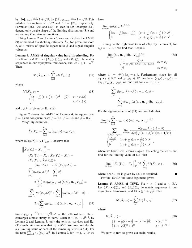
Using Lemma 2 and Lemma 3, we can calculate the AMSE(9) of the hard thresholding estimator Xλ, for given thresholdλ, at a matrix of specific aspect ratio β and signal singularvalues x:

Lemma 4. AMSE of singular value hard thresholding. Fixr > 0 and x ∈ Rr. Let {Xn(x)}∞n=1 and {Zn}∞n=1 be matrixsequences in our asymptotic framework, and let λ ≥ 1+

√β.

Then

M(Xλ,x) =

r∑i=1

M(Xλ, xi) (32)

where

M(Xλ, x) = (33){(x+ 1

x )(x+ βx )− (x2 − 2β

x2 ) x ≥ x∗(λ)x2 x < x∗(λ)

and x∗(λ) is given by Eq. (18).

Figure 2 shows the AMSE of Lemma 4, in square caseβ = 1 and nonsquare cases β = 0.1, β = 0.3 and β = 0.7.

Proof: By definition,

Xλ(Yn) =

mn∑i=1

ηH(yn,i;λ)un,i v′n,i ,

where ηH(y, τ) = y 1{y≥τ}. Observe that∣∣∣∣∣∣Xλ(Yn)−Xn

∣∣∣∣∣∣2F=

〈Xλ(Yn)−Xn , Xλ(Yn)−Xn〉 =〈Xλ(Yn) , Xλ(Yn)〉+〈Xn , Xn〉 − 2〈Xλ(Yn) , Xn〉 =

mn∑i=1

ηH(yn,i;λ)2 +

r∑i=1

x2i−

2

r∑i,j=1

xi ηH(yn,j ;λ) 〈aib′i , un,jv′n,j〉 =

mn∑i=r+1

ηH(yn,i;λ)2 +

r∑i=1

[ηH(yn,i;λ)

2 + x2i−

2xi

r∑j=1

ηH(yn,j ;λ) 〈aib′i , un,jv′n,j〉

]. (34)

Since yn,r+1a.s.−→ 1 +

√β < λ, the leftmost term above

converges almost surely to zero. When 0 ≤ xi ≤ β1/4, byLemma 2 and Lemma 3, only the term xi survives and Eq.(33) holds. Assume now that xi > β1/4. We now consider thea.s. limiting value of each of the remaining terms in (34). Forthe term

∑ri=1 ηH(yn,i;λ)

2, by Lemma 2, for i = 1, . . . , r we

have

limn→∞

ηH(yn,i;λ)2 a.s.={

(xi +1xi)(xi +

βxi) (xi +

1xi)(xi +

βxi) ≥ λ2

0 (xi +1xi)(xi +

βxi) < λ2

.

Turning to the rightmost term of (34), by Lemma 3, fori, j = 1, . . . , r we find that it equals

limn→∞

〈ai , un,j〉〈bi , v′n,j〉a.s.= (35)

1di

x4i−β

x3i

√(xi+β/xi)(xi+1/xi)

xi = xj

0 xi 6= xj

where di = # {j |xj = xi}. Furthermore, since for allx1,x2 ∈ Rm and y1,y2 ∈ Rn we have 〈x1y

′1 , x2y

′2〉 =

〈x1 , x2〉〈y1 , y2〉, we find that for i = 1, . . . , r,

r∑j=1

η(yn,j ;λ) 〈aib′i , un,jv′n,j〉 =

r∑j=1

η(yn,j ;λ) 〈ai , un,j〉〈bi , v′n,j〉 .

For the rightmost term of (34) we conclude that

limn→∞

xi

r∑j=1

η(yn,j ;λ) 〈ai′i , un,jv′n,j〉a.s.=

∑1≤j≤r : xj=xi

limn→∞

· η(yn,j ;λ) · (x4i − β)dix2i

√(xi + β/xi)(xi + 1/xi)

=

{x4i−βx2i

(xi +1xi)(xi +

βxi) ≥ λ2

0 (xi +1xi)(xi +

βxi) < λ2

,

where we have used Lemma 2 again. Collecting the terms, wefind for the limiting value of (34) that

limn→∞

∣∣∣∣∣∣Xλ(Yn)−Xn

∣∣∣∣∣∣2F

a.s.=

r∑i=1

M(Xλ, xi) , (36)

where M(Xλ, x) is given by (33) as required.For the TSVD, the same argument gives:

Lemma 5. AMSE of TSVD. Fix r > 0 and x ∈ Rr.Let {Xn(x)}∞n=1 and {Zn}∞n=1 be matrix sequences in ourasymptotic framework, and let λ ≥ 1 +

√β. Then

M(Xr,x) =

r∑i=1

M(Xr, xi) (37)

where

M(Xr, x) = (38){(x+ 1

x )(x+ βx )− (x2 − 2β

x2 ) x ≥ β1/4

(1 +√β)2 + x2 x ≤ β1/4

.

We now to turn to prove our main results.

11

Proof of Theorem 1: Let x∗ = x∗(λ∗(β)) where λ∗(β) isdefined in (11) and x∗(λ) is defined in (18). Then

x2∗ =

(x∗ +

1

x∗

)(x∗ +

β

x∗

)−(x2∗ −

2β

x2∗

).

It follows that for all x > 0 and λ ≥ 1 +√β,

M(Xλ∗ , x)

= min

{x2 ,

(x+

1

x

)(x+

β

x

)−(x2 − 2β

x2

)}≤M(Xλ, x)

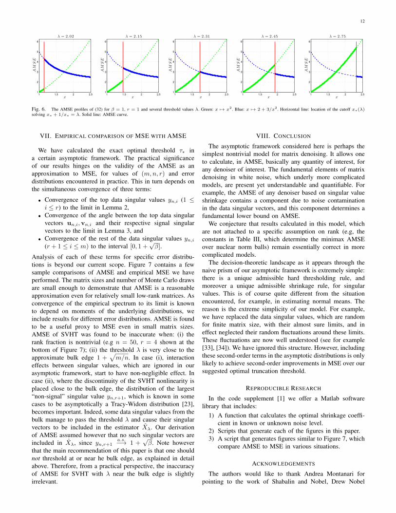
and the theorem follows from Eq. (32).Figure 6 provides a visual explanation of this proof for the

square (β = 1) case.Proof of Theorem 2: For x < β1/4, by Lemma 4 and

Lemma 5 we have

M(Xλ∗ , x) = x2 ≤ x2 + (1 +√β)2 =M(Xr, x) .

For x ≥ β1/4, by Lemma 5 and Theorem 1 we have

M(Xλ∗ , x) ≤M(Xr, x) .

Proof of Theorems 3 and 4: Theorem 3 is a special caseof Theorem 4. By (32), it is enough to consider the univariatefunction x 7→M(Xλ, x) defined in (33). The theorem followsfrom Lemma 4 using the following simple observation.

Let 0 < β ≤ 1 and λ > 1+√β. Denote by x∗(λ) the unique

positive solution to the equation (x + 1/x)(x + β/x) = λ2.Let λ∗ be the unique solution to the equation in λ

x4∗(λ)− (β + 1)x2∗ − 3β = 0 .

Then for the function M(Xλ, x) defined in (33), we have

argmaxx>0M(Xλ, x) = x∗(λ)

argminλ>1+√β maxx>0

M(Xλ, x) = λ∗

minλ>1+√β maxx>0

M(Xλ, x) = x∗(λ∗)2 .

Note that the least favorable situation occurs when x1 =. . . = xr = x∗(λ), and that x∗(λ) is precisely the value ofx for which the corresponding limiting data singular valuesatisfies yn,i

a.s.−→ λ. In other words, the least favorablesituation occurs when the data singular values all coincidewith each other and with the chosen hard threshold.

Proof of Lemma 1: Let Fn denote the empirical cumulativedistribution function (CDF) of the squared singular valuesof Yn. Write y2med,n = Median(Fn) where Median(·) isa functional which takes as argument the CDF and deliversthe median of that CDF. Under our asymptotic framework,almost surely, Fn converges weakly to a limiting distribution,FMP , the CDF of the Marcenko-Pastur distribution with shapeparameter β [21]. This distribution has a positive densitythroughout its support, in particular at its median. The medianfunctional is continuous for weak convergence at F0, andhence, almost surely,

y2med,n =Median(Fn)a.s.−→Median(F0) = µβ , n→∞ .

It follows that,

limn→∞

σ(Yn)

1/√n

a.s.= lim

n→∞

ymed,n√µβ

a.s.= 1 .

VI. GENERAL WHITE NOISE

Our results were formally stated for a sequence of modelsof the form Y = X + σZ, where X is a non-random matrixto be estimated, and the entries of Z are i.i.d samples froma distribution that is orthogonally invariant (in the sense thatthe matrix Z follows the same distribution as AZB, for anyorthogonal A ∈Mm,m and B ∈Mn,n). While Gaussian noiseis orthogonally invariant, many common distributions, whichone could consider to model white observation noise, are not.

One attractive feature of the discussion on optimal choiceof singular value hard threshold, presented above, is thatthe AMSE M(X,x) only depends on the signal matrix Xthrough its rank, or more specifically, through its nonzerosingular values x. If the distribution of Z is not orthogonallyinvariant, MSE (or AMSE) losses this property and dependson properties of X other than its rank. This point is discussedextensively in [22].

In general white noise, which is not necessarily orthogonallyinvariant, one can still allow MSE to depend on X onlythrough its singular values by placing a prior distribution onX and shifting to a model where it is a random, instead of afixed, matrix. Specifically, consider an alternative asymptoticframework to the one in Section II-B, in which the sequencedenoising problems Yn = Xn+Zn/

√n satisfies the following

assumptions:1) General white noise: The entries of Zn are i.i.d samples

from a distribution with zero mean, unit variance andfinite fourth moment.

2) Fixed signal column span and uniformly distributedsignal singular vectors: Let the rank r > 0 be fixedand choose a vector x ∈ Rr with coordinates x =(x1, . . . , xr). Assume that for all n,

Xn = Un diag(x1, . . . , xr, 0, . . . , 0)V′n (39)

is a singular value decomposition of Xn, where Unand Vn are uniformly distributed random orthogonalmatrices. Formally, Un and Vn are sampled from theHaar distribution on the m-by-m and n-by-n orthogonalgroup, respectively.

3) Asymptotic aspect ratio β: The sequence mn is suchthat mn/n→ β.

The second assumption above implies that Xn a “generic”choice of matrix with nonzero singular values x, or equiva-lently, a generic choice of coordinate systems in which thelinear operator corresponding to X is expressed.

The results of [25], which we have used, hold in this case aswell. It follows that Lemma 4 and Lemma 5, and consequentlyall our main results, hold under this alternative framework. Inshort, in general white noise, all our results hold if one iswilling to only specify the signal singular values, rather thanthe signal matrix, and consider a “generic” signal matrix withthese singular values.

12

1 1.5 2 2.51

2

3

4

5

6

x

AM

SE

λ = 2 .02

1 1.5 2 2.51

2

3

4

5

6

x

AM

SE

λ = 2 .15

1 1.5 2 2.51

2

3

4

5

6

x

AM

SE

λ = 2 .31

1 1.5 2 2.51

2

3

4

5

6

x

AM

SE

λ = 2 .45

1 1.5 2 2.51

2

3

4

5

6

x

AM

SE

λ = 2 .75

Fig. 6. The AMSE profiles of (32) for β = 1, r = 1 and several threshold values λ. Green: x 7→ x2. Blue: x 7→ 2 + 3/x2. Horizontal line: location of the cutoff x∗(λ)solving x∗ + 1/x∗ = λ. Solid line: AMSE curve.

VII. EMPIRICAL COMPARISON OF MSE WITH AMSE

We have calculated the exact optimal threshold τ∗ ina certain asymptotic framework. The practical significanceof our results hinges on the validity of the AMSE as anapproximation to MSE, for values of (m,n, r) and errordistributions encountered in practice. This in turn depends onthe simultaneous convergence of three terms:

• Convergence of the top data singular values yn,i (1 ≤i ≤ r) to the limit in Lemma 2,

• Convergence of the angle between the top data singularvectors un,i,vn,i and their respective signal singularvectors to the limit in Lemma 3, and

• Convergence of the rest of the data singular values yn,i(r + 1 ≤ i ≤ m) to the interval [0, 1 +

√β].

Analysis of each of these terms for specific error distribu-tions is beyond our current scope. Figure 7 contains a fewsample comparisons of AMSE and empirical MSE we haveperformed. The matrix sizes and number of Monte Carlo drawsare small enough to demonstrate that AMSE is a reasonableapproximation even for relatively small low-rank matrices. Asconvergence of the empirical spectrum to its limit is knownto depend on moments of the underlying distributions, weinclude results for different error distributions. AMSE is foundto be a useful proxy to MSE even in small matrix sizes.AMSE of SVHT was found to be inaccurate when: (i) therank fraction is nontrivial (e.g n = 50, r = 4 shown at thebottom of Figure 7); (ii) the threshold λ is very close to theapproximate bulk edge 1 +

√m/n. In case (i), interaction

effects between singular values, which are ignored in ourasymptotic framework, start to have non-negligible effect. Incase (ii), where the discontinuity of the SVHT nonlinearity isplaced close to the bulk edge, the distribution of the largest“non-signal” singular value yn,r+1, which is known in somecases to be asymptotically a Tracy-Widom distribution [23],becomes important. Indeed, some data singular values from thebulk manage to pass the threshold λ and cause their singularvectors to be included in the estimator Xλ. Our derivationof AMSE assumed however that no such singular vectors areincluded in Xλ, since yn,r+1

a.s.−→ 1 +√β. Note however

that the main recommendation of this paper is that one shouldnot threshold at or near he bulk edge, as explained in detailabove. Therefore, from a practical perspective, the inaccuracyof AMSE for SVHT with λ near the bulk edge is slightlyirrelevant.

VIII. CONCLUSION

The asymptotic framework considered here is perhaps thesimplest nontrivial model for matrix denoising. It allows oneto calculate, in AMSE, basically any quantity of interest, forany denoiser of interest. The fundamental elements of matrixdenoising in white noise, which underly more complicatedmodels, are present yet understandable and quantifiable. Forexample, the AMSE of any denoiser based on singular valueshrinkage contains a component due to noise contaminationin the data singular vectors, and this component determines afundamental lower bound on AMSE.

We conjecture that results calculated in this model, whichare not attached to a specific assumption on rank (e.g, theconstants in Table III, which determine the minimax AMSEover nuclear norm balls) remain essentially correct in morecomplicated models.

The decision-theoretic landscape as it appears through thenaive prism of our asymptotic framework is extremely simple:there is a unique admissible hard thresholding rule, andmoreover a unique admissible shrinkage rule, for singularvalues. This is of course quite different from the situationencountered, for example, in estimating normal means. Thereason is the extreme simplicity of our model. For example,we have replaced the data singular values, which are randomfor finite matrix size, with their almost sure limits, and ineffect neglected their random fluctuations around these limits.These fluctuations are now well understood (see for example[33], [34]). We have ignored this structure. However, includingthese second-order terms in the asymptotic distributions is onlylikely to achieve second-order improvements in MSE over oursuggested optimal truncation threshold.

REPRODUCIBLE RESEARCH

In the code supplement [1] we offer a Matlab softwarelibrary that includes:

1) A function that calculates the optimal shrinkage coeffi-cient in known or unknown noise level.

2) Scripts that generate each of the figures in this paper.3) A script that generates figures similar to Figure 7, which

compare AMSE to MSE in various situations.

ACKNOWLEDGEMENTS

The authors would like to thank Andrea Montanari forpointing to the work of Shabalin and Nobel, Drew Nobel

13

1 1.5 2 2.5 3 3.51

1.5

2

2.5

3

3.5

4

4.5

5

(20 , 20 , 1) gauss i an

x

MSE

X r

Xλ ∗

1 1.5 2 2.5 3 3.51

1.5

2

2.5

3

3.5

4

4.5

5

(20 , 20 , 1) be rnoul l i

xM

SE

X r

Xλ ∗

1 1.5 2 2.5 3 3.51

1.5

2

2.5

3

3.5

4

4.5

5

(20 , 20 , 1) uni form

x

MSE

X r

Xλ ∗

1 1.5 2 2.5 3 3.51

1.5

2

2.5

3

3.5

4

4.5

5

(20 , 20 , 1) student-t(6)

x

MSE

X r

Xλ ∗

1 1.5 2 2.5 3 3.51

1.5

2

2.5

3

3.5

4

4.5

5

(100 , 100 , 1) gauss i an

x

MSE

X r

Xλ ∗

1 1.5 2 2.5 3 3.51

1.5

2

2.5

3

3.5

4

4.5

5

(100 , 100 , 1) be rnoul l i

x

MSE

X r

Xλ ∗

1 1.5 2 2.5 3 3.51

1.5

2

2.5

3

3.5

4

4.5

5

(100 , 100 , 1) uni form

x

MSE

X r

Xλ ∗

1 1.5 2 2.5 3 3.51

1.5

2

2.5

3

3.5

4

4.5

5

(100 , 100 , 1) student-t(6)

x

MSE

X r

Xλ ∗

1 1.5 2 2.5 3 3.52

3

4

5

6

7

8

9

10

(50 , 50 , 2) gauss i an

x

MSE

X r

Xλ ∗

1 1.5 2 2.5 3 3.52

3

4

5

6

7

8

9

10

(50 , 50 , 2) be rnoul l i

x

MSE

X r

Xλ ∗

1 1.5 2 2.5 3 3.52

3

4

5

6

7

8

9

10

(50 , 50 , 2) uni form

x

MSE

X r

Xλ ∗

1 1.5 2 2.5 3 3.52

3

4

5

6

7

8

9

10

(50 , 50 , 2) student-t(6)

x

MSE

X r

Xλ ∗

1 1.5 2 2.5 3 3.54

6

8

10

12

14

16

18

20

(50 , 50 , 4) gauss i an

x

MSE

X r

Xλ ∗

1 1.5 2 2.5 3 3.54

6

8

10

12

14

16

18

20

(50 , 50 , 4) be rnoul l i

x

MSE

X r

Xλ ∗

1 1.5 2 2.5 3 3.54

6

8

10

12

14

16

18

20

(50 , 50 , 4) uni form

x

MSE

X r

Xλ ∗

1 1.5 2 2.5 3 3.54

6

8

10

12

14

16

18

20

(50 , 50 , 4) student-t(6)

x

MSE

X r

Xλ ∗

Fig. 7. The AMSE (solid line) and empirical MSE (circles) of TSVD Xr and optimal SVHT Xλ∗ for β = 1 and signal singular value x ≥ 1 which correspond to leadingdata singular values that fall beyond the bulk egde. In a given panel, for a given value of x, the blue and the red dots were generated by first generating a signal matrix X , andthen averaging each of the losses

∣∣∣∣∣∣X(X + Z/√n)−X

∣∣∣∣∣∣2F

over the same 50 Monte Carlo draws of the noise matrix Z. Each column of panels represents a different noisewith zero mean and unit variance: Gaussian, Bernoulli on ±1, uniform on [−0.5, 0.5] and Student’s t-distribution with 6 degreees of freedom; Panel titles indicate (m,n, r)and the noise distribution. Top rows: r = 1, different values of m = n. Bottom rows: m = n = 50, different values of r (for r > 1, signal singular values are all equal).Reproducibility advisory: script to generate figure, and to perform similar experiments, is included in code supplement [1].

and Sourav Chatterjee for helpful discussions, Art Owen forpointing to the work of Perry, and the anonymous referees for

their useful suggestions. This work was partially supportedby NSF DMS 0906812 (ARRA). MG was partially supported

14

by a William R. and Sara Hart Kimball Stanford GraduateFellowship.

REFERENCES

[1] D. L. Donoho and M. Gavish, “Code supplement to ‘TheOptimal Hard Threshold for Singular Values is 4/

√3’,”

http://purl.stanford.edu/vg705qn9070, 2014, accessed 27 March 2014.[Online]. Available: http://purl.stanford.edu/vg705qn9070

[2] G. Golub and W. Kahan, “Calculating the Singular Values andPseudo-Inverse of a Matrix,” Journal of the Society for Industrial &Applied Mathematics: Series B, vol. 2, no. 2, pp. 205–224, 1965.

[3] C. Eckart and G. Young, “The approximation of one matrix by anotherof lower rank,” Psychometrika, vol. 1, no. 3, 1936.

[4] O. Alter, P. Brown, and D. Botstein, “Singular value decomposition forgenome-wide expression data processing and modeling,” Proceedings ofthe National Academy of Sciences, vol. 97, no. 18, pp. 10 101–10 106,Aug. 2000.

[5] D. Jackson, “Stopping rules in principal components analysis: acomparison of heuristical and statistical approaches,” Ecology, 1993.Available: http://www.jstor.org/stable/10.2307/1939574

[6] T. D. Lagerlund, F. W. Sharbrough, and N. E. Busacker, “Spatialfiltering of multichannel electroencephalographic recordings throughprincipal component analysis by singular value decomposition.”Journal of clinical neurophysiology : official publication of theAmerican Electroencephalographic Society, vol. 14, no. 1, pp. 73–82,Jan. 1997.

[7] A. L. Price, N. J. Patterson, R. M. Plenge, M. E. Weinblatt, N. a.Shadick, and D. Reich, “Principal components analysis corrects forstratification in genome-wide association studies.” Nature genetics,vol. 38, no. 8, pp. 904–9, Aug. 2006.

[8] O. Edfors and M. Sandell, “OFDM channel estimation by singularvalue decomposition,” IEEE Transactions on Communications, vol. 46,no. 7, pp. 931-939, 1998.

[9] R. Cattell, “The scree test for the number of factors,” Multivariatebehavioral research, 1966.

[10] S. Wold, “Cross-Validatory Estimation of the Number of Componentsin Factor and Principal Components Components Models,”Technometrics, vol. 20, no. 4, pp. 397–405, 1978. [Online]. Available:http://www.tandfonline.com/doi/pdf/10.1080/00401706.1978.10489693

[11] P. D. Hoff, “Model averaging and dimension selection for thesingular value decomposition,” Sep. 2006. [Online]. Available:http://arxiv.org/abs/math/0609042

[12] A. B. Owen and P. O. Perry, “Bi-cross-validation of the SVDand the nonnegative matrix factorization,” The Annals of AppliedStatistics, vol. 3, no. 2, pp. 564–594, Jun. 2009. [Online]. Available:http://projecteuclid.org/euclid.aoas/1245676186

[13] P. O. Perry, “Cross validation for unsupervised learning,” PhD Thesis,Department of Statistics, Stanford University, 2009. [Online]. Available:http://http://arxiv.org/abs/0909.3052

[14] D. Achlioptas and F. McSherry, “Fast Computation of Low RankMatrix Approximations,” in Proceedings of the thirty-third annual ACMsymposium on Theory of computing, 2001, pp. 611–618. [Online].Available: http://dl.acm.org/citation.cfm?id=380858

[15] Y. Azar, A. Fiat, A. R. Karlin, F. McSherry, and J. Saia, “SpectralAnalysis of Data,” in Proceedings of the thirty-third annual ACMsymposium on Theory of computing, 2001, pp. 619–626. [Online].Available: http://dl.acm.org/citation.cfm?id=380859

[16] P. J. Bickel and E. Levina, “Covariance regularization by thresholding,”The Annals of Statistics, vol. 36, no. 6, pp. 2577–2604, Dec. 2008.[Online]. Available: http://projecteuclid.org/euclid.aos/1231165180

[17] S. Chatterjee, “Matrix estimation by universal singular valuethresholding,”, 2010. [Online]. Available: arxiv.org/abs/1212.1247

[18] R. H. Keshavan and S. Oh, “OptSpace : A Gradient Descent Algorithmon the Grassman Manifold for Matrix Completion,” 2009. [Online].Available: arxiv.org/abs/0910.5260

[19] R. H. Keshavan, A. Montanari, and S. Oh, “Matrix completionfrom a few entries,” IEEE Transcations on Information Theory,vol. 56, no. 6, pp.2980-2998, 2010. [Online]. Available:http://ieeexplore.ieee.org/xpls/abs all.jsp?arnumber=5466511

[20] J. Tanner and K. Wei, “Normalized iterative hard thresh-olding for matrix completion,” 2012. [Online]. Available:http://people.maths.ox.ac.uk/tanner/papers/TaWei NIHT.pdf

[21] Z. Bai, and J. W. Silverstein, “Spectral Analysis of LargeDimensional Random Matrices (2nd Edition),” 2010. Springer NewYork. doi:10.1007/978-1-4419-0661-8

[22] A. Shabalin and A. Nobel, “Reconstruction of a Low-rank Matrix inthe Presence of Gaussian Noise,” Journal of Multivariate Analysis,vol. 118, pp. 67–76, 2013.

[23] I. M. Johnstone, “On the distribution of the largest eigenvalue inprincipal components analysis,” Annals of Statistics, vol. 29, no. 2, pp.295–327, 2001.

[24] D. L. Donoho, M. Gavish and I. M. Johnstone, “Optimal Shrinkageof Eigenvalues in the Spiked Covariance Model,” Stanford UniversityStatistics Department technical report 2013-10, 2013. [Online].Available: http://arxiv.org/abs/1311.0851

[25] F. Benaych-Georges and R. R. Nadakuditi, “The singular values andvectors of low rank perturbations of large rectangular random matrices,”Journal of Multivariate Analysis, vol. 111, pp. 120–135, Oct. 2012.

[26] Y. Q. Yin, Z. D. Bai, and P. R. Krishnaiah, “On the limit of thelargest eigenvalue of the large dimensional sample covariance matrix,”Probability Theory and Related Fields, vol. 78, pp. 509-521, 1988.

[27] Y. Q. Yin, Z. D. Bai, “Limit of the smallest eigenvalue of a largedimensional sample covariance matrix,” The annals of Probability,vol. 21, no. 3, pp.1275-1294, 1993.

[28] M. Gavish and D. L. Donoho, “Optimal Shrinkage of Singular Values,”Stanford University Statistics Department technical report 2014-08,2014. [Online]. Available: http://arxiv.org/abs/1405.7511

[29] J.-F. Cai, E. J. Candes, and Z. Shen, “A Singular ValueThresholding Algorithm for Matrix Completion,” SIAM Journalon Optimization, vol. 20, no. 4, p. 1956, 2008. [Online]. Available:http://arxiv.org/abs/0810.3286

[30] E. J. Candes, C. A. Sing-long, and J. D. Trzasko, “Unbiased RiskEstimates for Singular Value Thresholding and Spectral Estimators,”IEEE Transactions on Signal Processing, vol. 61, no. 19, pp.4643–4657, 2012.

[31] D. L. Donoho and M. Gavish, “Minimax Risk of Matrix Denoisingby Singular Value Thresholding,” Stanford University StatisticsDepartment technical report 2013-03, 2013. [Online]. Available:http://arxiv.org/abs/1304.2085

[32] S. Kritchman and B. Nadler, “Non-parametric detection of the numberof signals: Hypothesis testing and random matrix theory,” SignalProcessing, IEEE Transactions, vol. 57, no. 10, pp. 3930–3941, 2009.

[33] Z. Bai and J.-f. Yao, “Central limit theorems for eigenvalues in aspiked population model,” Annales de l’Institut Henri Poincare (B)Probability and Statistics, vol. 44, no. 3, pp. 447–474, Jun. 2008.

[34] D. Shi, “Asymptotic Joint Distribution of Extreme Sample Eigenvaluesand Eigenvectors in the Spiked Population Model,” Apr. 2013. [Online].Available: http://arxiv.org/abs/1304.6113

Matan Gavish received the dual B.Sc. degree inMathematics and Physics from Tel Aviv University(TAU) in 2006 and the M.Sc. degree in Mathematicsfrom the Hebrew University of Jerusalem in 2008.He is currently a doctoral student in Statistics atStanford University, in collaboration with the YaleUniversity program in Applied Mathematics. Hisresearch interests include applied harmonic analysis,high-dimensional statistics and computing. He wasin the Adi Lautman Interdisciplinary Program foroutstanding students at TAU from 2002 to 2006 and

held a William R. and Sara Hart Kimball Stanford Graduate Fellowship from2009 to 2012.

David L. Donoho is a professor at Stanford Uni-versity. His research interests include computationalharmonic analysis, high-dimensional geometry, andmathematical statistics. Dr. Donoho received thePh.D. degree in Statistics from Harvard Univer-sity, and holds honorary degrees from University ofChicago and Ecole Polytechnique Federale de Lau-sanne. He is a member of the American Academyof Arts and Sciences and the US National Academyof Sciences, and a foreign associate of the FrenchAcademie des sciences.