The one-component plasma: a conceptual approach

arX

iv:c

ond-

mat

/981

0213

v2 [

cond

-mat

.sof

t] 2

1 Ja

n 19

99

The one-component plasma: a conceptual

approach

M.N. Tamashiro, 1 Yan Levin 2 and Marcia C. Barbosa

Instituto de Fısica, Universidade Federal do Rio Grande do Sul, Caixa Postal15051, 91501-970 Porto Alegre (RS), Brazil

Abstract

The one-component plasma (OCP) represents the simplest statistical mechanicalmodel of a Coulomb system. For this reason, it has been extensively studied overthe last forty years. The advent of the integral equations has resulted in a dramaticimprovement in our ability to carry out numerical calculations, but came at theexpense of a physical insight gained in a simpler analytic theory. In this paper wepresent an extension of the Debye-Huckel (DH) theory to the OCP. The theoryallows for analytic calculations of all the thermodynamic functions, as well as thestructure factor. The theory explicitly satisfies the Stillinger-Lovett and, for smallcouplings, the compressibility sum rules, implying its internal self consistency.

Key words: One-component plasma, electrolytes, structure factors, Debye-Huckeltheory.

1 Introduction

The classical one-component plasma (OCP) is an idealized system of N identical point-particlesof charge q, in a uniform neutralizing background of dielectric constant D [1,2]. For concretenesswe shall suppose that the particles are positively charged, while the background is negative.Each ion, inside the volume V , is assumed to interact with the others exclusively through theCoulomb potential. The OCP has been extensively studied because it serves as the simplestpossible model for a variety of important physical systems, ranging from electrolytes and charge-stabilized colloids [3] to the dense stellar matter [4]. With the advent of powerful computers andnew developments in the liquid-state theory our ability to perform thermodynamic calculationson this model has seen a dramatic improvement characterized, in particular, by the quantitative

1 Present address: Materials Research Laboratory, University of California at Santa Barbara, 93106-5130 Santa Barbara (CA), USA; e-mail: [email protected] Corresponding author, e-mail: [email protected].

Preprint submitted to Elsevier Preprint 1 February 2008

agreement between the integral-equations based theories of the OCP and the Monte Carlo(MC) simulations [5]. Unfortunately, the intrinsic complexity of the integral equations, insteadof clarifying the underlying physics, tends to obscure it. This should be contrasted with thesimplicity and the transparency of the Debye-Huckel (DH) theory [6], which allows for a veryclear physical picture of an ionic solution.

Let us recall the early history of electrolyte solutions. The first modern ideas about electrolytescan be traced to the pioneering work of the swedish physicist Svante Arrhenius [7] at the endof the last century. In particular, it was Arrhenius who realized that when salts and acids aredissolved in a polar solvent, the molecules become dissociated, producing cations and anions.Arguing from what can now be called mean-field point of view, Arrhenius concluded that, sincethe electrolyte solution is charge neutral and the ions are uniformly distributed, the average forceacting on each particle is null. All the nontrivial characteristics of the electrolytes Arrheniusattributed to the incomplete dissociation of the molecules. In this simple picture an electrolyteis treated as an ideal gas composed of three species, cations, anions, and neutral molecules,whose densities are controlled by the law of mass action. All the electrostatic interactions areneglected except in as far as treating the cations and the anions as distinct entities. This simpletheory has proven to work quite well for what are now known as weak electrolytes, such asBrønsted acids and bases. In the case of strong electrolytes, such as NaCl or HCl, the theoryproved seriously flawed. It took almost forty years before a satisfactory solution could be found.It appeared in the form of the now famous DH theory of strong electrolytes [6]. The great insightof Debye and Huckel was to realize that although the ions are on average uniformly distributedinside the solution, due to the long-range Coulomb force there exist strong correlations in thepositions of the positively and the negatively charged particles; evidently in the vicinity of apositive ion there will be an excess of negative particles and vice-versa.

To make this idea concrete and to see how it applies to the OCP, let us fix one mobile ion atthe origin and ask what is the induced electrostatic potential in its surrounding. Clearly thismust satisfy the Poisson equation,

∇2φ(r) = −4π

D(r). (1)

To find the closure to this equation, we shall follow DH and suppose that the rest of the mobileions arrange themselves in accordance with the Boltzmann distribution,

(r) = qρ+ exp [−βqφ(r)] − qρ−, (2)

where ρ+ = N/V is the average density of the mobile ions, ρ− is the density of the uniformneutralizing background, and β = 1/kBT . The next step of the DH theory is to linearize theexponential factor, leading to

(r) = −Dκ2D

4πφ(r), (3)

where κD =√

4πλBρ+ and λB = βq2/D are the inverse Debye screening and the Bjerrum

2

lengths, respectively. Clearly, the linearization can only be justified in the high-temperature(weak-coupling) limit. The resulting Helmholtz equation, ∇2φ(r) = κ2

Dφ(r), can be easilyintegrated to produce a potential of the Yukawa form. The fundamental lesson of DH is thatthe ions arrange themselves in such a way as to screen the long-range Coulomb interaction. Itis this renormalization of the interaction potential that is responsible for the existence of thethermodynamic limit for Coulomb systems. However, not everything is rosy with this simpletheory. It is sufficient to look at the charge-density distribution,

(r) = −qκ2D

4πre−κDr, (4)

to notice that something went seriously wrong.

Clearly, the physical restriction that (r) ≥ −qρ− is strongly violated in the region near thefixed ion. The problem can be traced back to the linearization of the Boltzmann factor, whichis unjustified at short distances, since there the electrostatic potential is not small even forhigh temperatures. Fortunately, not all is lost. A simple solution to overcome this difficultywas suggested by Nordholm [8], who proposed an augmentation of the DH theory to includean effective spherical cavity around the fixed ion, inside which no other ions can penetrate.The presence of such a cavity is quite reasonable, since the electrostatic repulsion between thelike-charged ions should prevent them from coming into close contact. Furthermore, we canestimate the size of the hole, h, by comparing the repulsive Coulomb energy with the kineticthermal energy, q2/Dh ∼ kBT , or h ∼ q2/DkBT . Evidently, the higher the temperature, thesmaller the size of the exclusion region. This, of course, is intuitive, since at higher temperaturesthe ions will have more kinetic energy to overcome the mutual repulsion. A more consistentway of defining the hole size h is to require an overall charge neutrality [8], or, equivalently,the continuity of the potential and of the electric field across the hole boundary. Performing asimple calculation, we find

h= d [ω(Γ) − 1] /√

3Γ, (5)

ω(Γ)=[

1 + (3Γ)3/2]1/3

, (6)

where we have defined the usual coupling constant for the OCP, Γ = βq2/Dd, and d is the

characteristic length scale, d =(

4πρ3+/3

)−1. In the low-coupling limit this reduces to the

energetically determined expression for the size of the cavity, h ≈ λB. Nordholm was able todemonstrate that this Debye-Huckel plus hole (DHH) theory produces an equation of state forthe OCP which is in good agreement with the MC simulations. The question, however, stillremains to what extent the hole is a physical object or just a convenient mathematical trickto correct for the linearization of the Poisson-Boltzmann (PB) equation. Clearly, if the cavitypostulated by the DHH theory is real, the best way to study it is by considering the structurefactor. In particular, if everything is all right with the DHH theory, the structure factor obtainedon its basis should be in good agreement with the MC simulations. Unfortunately, it is wellknown that the traditional ways of obtaining the correlation functions out of the DH theorylead to expressions which are seriously flawed [9]. In the case of the restricted primitive model(RPM), equisized spheres carrying charges ±q, the correlation functions violate the well-known

3

Stillinger-Lovett sum rules [10] and do not reproduce the charge-density oscillations known toexist at high densities [11].

Recently Lee and Fisher [9] have proposed an extension of the DH theory of strong elec-trolytes to nonuniform densities. The generalized DH theory (GDH) allows the calculationof the density-density and of the charge-charge correlation functions in a most natural way,through a functional differentiation of the free-energy functional. Furthermore, since the theoryis constructed at the level of free energy, it is internally self consistent, as can be judged bythe various sum rules that it satisfies. This, of course, is a great advantage over the traditionalintegral-equations based theories, which are constructed at the level of the correlation functionsand depend on the route taken to the thermodynamics [12], i.e. virial, compressibility, etc. Thecomparison of the GDH theory with experiments or simulations, however, is made difficult bythe same flaw (or virtue, depending on how one looks at it) that the original DH theory suffers,its linearity. The linearity of the DH theory for electrolytes is both a blessing and a curse. Itensures the internal self consistency of the theory, but is also responsible for undercounting theconfigurations in which the oppositely charged ions come into a close contact, forming dipolarpairs. It was shown recently how this difficulty can be overcome in the context of the Debye-Huckel-Bjerrum (DHBj) theory [13], by allowing for the existence of a chemical equilibriumbetween the monopoles and dipoles. Unfortunately this stratagem is difficult to implement inthe case of the GDH theory. The goal of this paper, then, is two-fold: test the physical natureof the cavity in the DHH theory and, by apply the GDH theory to the OCP — which is freefrom the cluster formations that plague RPM — test the extent of its validity.

2 The generalized Debye-Huckel theory for the one-component plasma

The DHH theory for the OCP is extended to allow for a nonuniform, slowly varying ionicdensity,

ρ+(r) = ρ+ (1 + ∆ cosk · r) . (7)

The negative background, as in the original OCP theory, is maintained uniform,

ρ−(r) = ρ−, ∀r. (8)

To preserve the electroneutrality on long-length scales, the overall equilibrium densities mustbe equal, ρ+ = ρ−.

The Helmholtz free-energy, F , is a functional of the ionic density ρ+(r). The direct correlationfunction, C++(r1 − r2), is defined in terms of the second derivative of the excess free energy,

C++(r1 − r2)≡−β δ2 {F [ρ+(r)] − Fideal [ρ+(r)]}δρ+(r1) δρ+(r2)

∣

∣

∣

∣

∣

ρ+(r)=ρ+

4

=δ(r1 − r2)

ρ+

− βδ2F [ρ+(r)]

δρ+(r1) δρ+(r2)

∣

∣

∣

∣

∣

ρ+(r)=ρ+

. (9)

Here, Fideal [ρ+(r)] is the usual ideal-gas Helmholtz free-energy functional,

βFideal [ρ+(r)] =∫

d3r′ ρ+(r′){

ln[

ρ+(r′)Λ3]

− 1}

, (10)

where Λ is the thermal de Broglie wavelength.

The direct correlation function is connected with the total correlation function, H(r), throughthe Ornstein-Zernike relation,

H(r) = C++(r) + ρ+

∫

d3r′ C++(r − r′)H(r′), (11)

which in the Fourier space can be written as

H(k) =C++(k)

1 − ρ+C++(k), (12)

where C++(k) and H(k) are the Fourier transforms of the direct and the total correlationfunctions, respectively,

C++(k) =∫

d3r C++(r) exp (ik · r) , (13)

H(k) =∫

d3r H(r) exp (ik · r) . (14)

The structure factor is defined as

S(k) ≡ 1 + ρ+H(k) =1

1 − ρ+C++(k). (15)

Evidently, the knowledge of the direct correlation function C++(r) is equivalent to the knowl-edge of the structure factor S(k).

To proceed, we impose an infinitesimal variation on the mobile-ion density, Eq. (7), and expandthe reduced Helmholtz free-energy functional density, f ≡ βF/V , in powers of ∆. To secondorder, the variation δf can be written as (see details in appendix B)

δf [ρ+(r)] ≡ f [ρ+(r)] − f [ρ+] = βµρ+∆δk0 +1

4S−1(k)ρ+∆2 (1 + δk0) , (16)

where βµ = ∂f/∂ρ+ is the equilibrium chemical potential, δk0 = 1V

(2π)3δ3(k) is the Kroneckerdelta and δ3(k) is the three-dimensional Dirac delta function. The free-energy density of the

5

homogeneous reference system, f [ρ+], is obtained by setting ∆ = 0 in the expression forf [ρ+(r)]. Clearly, if we are able to construct the free-energy functional for a nonuniform system,the structure factor, S(k), can be read directly from the second-order term.

We proceed in a way exactly analogous to the usual DH theory. Let us fix one positive ion atr′ and ask what is the electrostatic potential, φ(r, r′), at a point r in its surrounding. We shallassume that, just like in the uniform case, this potential satisfies the PB equation,

∇2rφ(r, r′) =−4πq

D

{

δ3(r − r′) + ρ+(r) exp[

−βqφ(r, r′)]

− ρ−(r)}

. (17)

A crucial point to remark [9] is that the potential which appears in the Boltzmann factor of (17),φ(r, r′), represents a local-induced potential,

φ(r, r′) ≡ φ(r, r′) − Φ(r), (18)

obtained by extracting from the total potential φ(r, r′) an imposed electrostatic potential, Φ(r),produced by the neutralizing background and the imposed charge-density variation (7),

∇2Φ(r) = −4πq

D[ρ+(r) − ρ−] = −4πqρ+

D∆ cos k · r, ∀r. (19)

With the separation of the total potential φ(r, r′) into two parts, the Helmholtz free-energyfunctional can be written as

F [ρ+(r)] = Fideal [ρ+(r)] + Fimposed [ρ+(r)] + Finduced [ρ+(r)] , (20)

where the excess free energies are obtained through the Debye charging process [6,9],

Fimposed [ρ+(r)]= q∫

d3r′ [ρ+(r′) − ρ−]

1∫

0

dλΦ(r′, λq), (21)

Finduced [ρ+(r)]= q∫

d3r′ ρ+(r′)

1∫

0

dλψ(r′, λq). (22)

In Eq. (22), ψ(r′) is the mean induced electrostatic potential felt by the positive ion fixed atr′,

ψ(r′) ≡ limr→r′

[

φ(r, r′) − q

D|r − r′|

]

. (23)

Linearization of the Boltzmann factor of (17) results in the GDH equation for the inducedpotential,

6

∇2rφ(r, r′) =−4πq

D

[

δ3(r − r′) − ρ+(r)]

=−4πq

D

[

δ3(r − r′) − ρ+(1 + ∆ cosk · r)]

, for |r − r′| ≤ h, (24)

∇2rφ(r, r′) =

4πβq2ρ+(r)

Dφ(r, r′)

=κ2D (1 + ∆ cosk · r) φ(r, r′), for |r − r′| ≥ h. (25)

As discussed in the introduction, to prevent the unphysical artifacts of the linearization ofthe PB equation, we have explicitly introduced a cavity h around the fixed ion at r′, givenby Eq. (5), into which no other mobile ions can penetrate.

In the following subsections we shall obtain the contributions to the variation of the free-energydensity.

2.1 The ideal-gas contribution

The ideal-gas contribution is given by (10) with the imposed mobile-ion charge distribution (7).Expanding (10) up to order ∆2 and using the integrals (A.3) and (A.4), we obtain the ideal-gascontribution to the variation of the reduced free-energy density,

δfideal [ρ+(r)] = ln(

ρ+Λ3)

ρ+∆δk0 +1

4ρ+∆2 (1 + δk0) . (26)

2.2 The imposed electrostatic potential contribution

The imposed electrostatic potential satisfies the Poisson equation (19), whose formal solutioncan be written as

Φ(r) =qρ+

D∆∫

d3r′ cos k · r′

|r − r′| . (27)

The contribution to the Helmholtz free-energy functional is obtained through the Debye charg-ing process [6],

Fimposed [ρ+(r)]= q∫

d3r′ [ρ+(r′) − ρ−]

1∫

0

dλΦ(r′, λq)

=q2ρ2

+

D∆2

∫

d3r d3r′ cos k · r cos k · r′

|r − r′|

1∫

0

dλ λ. (28)

In this case the charging merely produces a trivial factor of 1/2 and using the integral (A.7), weobtain the contribution of the imposed electrostatic potential to the variation of the reduced

7

free-energy density,

δfimposed [ρ+(r)] =1

4

(

κD

k

)2

ρ+∆2(1 + δk0) . (29)

2.3 The induced electrostatic potential contribution

The induced electrostatic potential satisfies the GDH equation, given by (24) and (25). It isconvenient to rewrite them in a spherical coordinate system centered on the positive ion fixedat r′. Introducing the difference vector

R = r − r′, (30)

the GDH equation for the induced potential reads

∇2Rφ(R + r′, r′) =

−4πqD {δ3(R) − ρ+ [1 + ∆ cos k · (R + r′)]} , for |R| ≤ h,

κ2D [1 + ∆ cos k · (R + r′)] φ(R + r′, r′), for |R| ≥ h.

(31)

Using the Green’s function G (R,R′) associated with (31) derived in appendix C, it can betransformed into the integral equation

φ(r, r′) = φ(R + r′, r′) =1

D

∫

d3R′ (R′)G (R,R′) , (32)

where the effective charge density, (R), is given by

(R)=

qδ3(R) − qρ+ [1 + ∆ cos k · (R + r′)] , for R ≤ h,

−D

4πκ2

Dφ (R + r′, r′) ∆ cos k · (R + r′), for R ≥ h.(33)

This equation can be solved perturbatively in powers of ∆ (see appendix D).

The mean induced electrostatic potential felt by the positive ion fixed at r′,

ψ(r′) = limR→0

[

φ(R + r′, r′) − q

DR

]

, (34)

can be written, to order ∆2, as (see derivation in appendix D)

βqψ(r′)=−1

2x(x+ 2) − ∆ cos k · r′

[

1

α2− sinαx

α3(1 + x)− cosαx

α2(1 + x)+

x

1 + xI+

0 (x, α)

]

8

+1

α(1 + x)∆2

∞∑

ℓ=0

(2ℓ+ 1) cos2(

k · r′ + ℓπ

2

)

xℓ+2jℓ+1(αx)

gℓ+1(x)I+

ℓ (x, α)

+x

1 + x∆2

∞∑

ℓ=0

(−1)ℓ+1 (2ℓ+ 1) cos2(

k · r′ + ℓπ

2

)

×{

1

2

gℓ+1(−x)gℓ+1(x)

[

I+ℓ (x, α)

]2+ I+

ℓ (x, α)I−ℓ (x, α) − I0

ℓ (x, α)

}

. (35)

where x = κDh, α = k/κD, jℓ(ξ) is the spherical Bessel function of the first kind,

jℓ(ξ) =

√

π

2ξJℓ+1/2(ξ), (36)

gℓ(ξ) is the ℓ-th grade polynomial associated with the modified spherical Bessel function of thethird kind, kℓ(ξ),

gℓ(ξ) ≡ eξξℓ+1kℓ(ξ) =ℓ∑

m=0

Γ(ℓ+m+ 1)

2mm! Γ(ℓ−m+ 1)ξℓ−m =

ℓ∑

m=0

(2m)!

2mm!

(

ℓ+m

2m

)

ξℓ−m, (37)

where Γ(m) = (m−1)! is the Euler gamma function, and {Iνℓ }, ν = ±, 0, are the one-dimensional

quadratures

I−ℓ (s, α)=

s∫

0

dξ ξ−ℓgℓ(−ξ)jℓ(αξ), (38)

I0ℓ (x, α)=

∞∫

x

ds s−ℓgℓ(s)jℓ(αs)I−ℓ (s, α) exp [2(x− s)] , (39)

I+ℓ (x, α)=

∞∫

x

ds s−ℓgℓ(s)jℓ(αs) exp [2(x− s)] . (40)

The contribution to the Helmholtz free-energy functional is obtained through the Debye charg-ing process [6,9],

Finduced [ρ+(r)]= q∫

d3r′ ρ+(r′)

1∫

0

dλψ(r′, λq)

= qρ+

∫

d3r′ (1 + ∆ cosk · r′)

1∫

0

dλψ(r′, λq), (41)

which yields the reduced free-energy density,

finduced [ρ+(r)] = ρ+f0 +[

f0 +1

2f1(α)

]

ρ+∆δk0 +1

4[f1(α) + f2(α)] ρ+∆2 (1 + δk0) , (42)

9

from which the variation follows,

δfinduced [ρ+(r)]= finduced [ρ+(r)] − finduced [ρ+]

=[

f0 +1

2f1(α)

]

ρ+∆δk0 +1

4[f1(α) + f2(α)] ρ+∆2 (1 + δk0) , (43)

where

f0 =−1

2

1∫

0

dλ

λxλ(xλ + 2) = −1

2

ω∫

1

dωλω2

λ (ωλ + 1)

ω2λ + ωλ + 1

=1

4

[

1 − ω2 +2π

3√

3+ ln

(

ω2 + ω + 1

3

)

− 2√3

tan−1

(

2ω + 1√3

)]

, (44)

f1(α)=− 1

α2+

2

α3

1∫

0

dλλ2

ωλsin(αxλ/λ) +

2

α2

1∫

0

dλλ

ωλcos(αxλ/λ)

− 2

1∫

0

dλ

λ

ωλ − 1

ωλ

I+0 (xλ, α/λ), (45)

f2(α)=∞∑

ℓ=0

(2ℓ+ 1)

[

1 + (−1)ℓδk0

1 + δk0

]

2

α

1∫

0

dλxℓ+2

λ jℓ+1(αxλ/λ)

ωλ gℓ+1(xλ)I+

ℓ (xλ, α/λ)

+ (−1)ℓ+1

1∫

0

dλ

λ

ωλ − 1

ωλ

[

gℓ+1(−xλ)

gℓ+1(xλ)

[

I+ℓ (xλ, α/λ)

]2

+ 2I+ℓ (xλ, α/λ)I−

ℓ (xλ, α/λ) − 2I0ℓ (xλ, α/λ)

]

, (46)

xλ =ωλ − 1, (47)

ωλ =[

1 + λ3 (3Γ)3/2]1/3

, (48)

ω=ωλ=1 =[

1 + (3Γ)3/2]1/3

. (49)

We note that the reduced induced free-energy density for the reference system,

finduced [ρ+] = ρ+f0

=1

4ρ+

[

1 − ω2 +2π

3√

3+ ln

(

ω2 + ω + 1

3

)

− 2√3

tan−1

(

2ω + 1√3

)]

, (50)

is the same as the one previously obtained by Nordholm [8].

10

3 Analytical results and the sum rules

Collecting all the contributions to the variation of the reduced free-energy density,

δf [ρ+(r)] = δfideal [ρ+(r)] + δfimposed [ρ+(r)] + δfinduced [ρ+(r)] , (51)

and comparing with the expansion given by (16), we obtain the equilibrium chemical potential,

βµ = ln(

ρ+Λ3)

+ f0 +1

2limα→0

f1(α) = ln(

ρ+Λ3)

+ f0 +1

12

(

1 − ω2)

, (52)

which corresponds to the usual OCP chemical potential [8], and the structure factor,

S−1(k) = 1 +2

α3

1∫

0

dλλ2

ωλsin(αxλ/λ) +

2

α2

1∫

0

dλλ

ωλcos(αxλ/λ)

− 2

1∫

0

dλ

λ

ωλ − 1

ωλ

I+0 (xλ, α/λ)

+∞∑

ℓ=0

(2ℓ+ 1)

2

α

1∫

0

dλxℓ+2

λ jℓ+1(αxλ/λ)

ωλ gℓ+1(xλ)I+

ℓ (xλ, α/λ)

+ (−1)ℓ+1

1∫

0

dλ

λ

ωλ − 1

ωλ

[

gℓ+1(−xλ)

gℓ+1(xλ)

[

I+ℓ (xλ, α/λ)

]2

+ 2I+ℓ (xλ, α/λ)I−

ℓ (xλ, α/λ) − 2I0ℓ (xλ, α/λ)

]

. (53)

This is the central result of this paper, the explicit expression for the structure factor of theOCP, given in terms of an infinite series. To check the internal consistency of the theory, weexplore how well it satisfies various known sum rules. All these can be conveniently summarizedin the exact, small k expansion of the structure factor [2],

S−1exact(k) =

(

κD

k

)2

+β

ρ+χ+ O(k2), (54)

where χ is the compressibility of the OCP. The first term is the result of the charge neutralityand of the Stillinger-Lovett second-moment condition [10], while the second term corresponds tothe fourth-moment or the “compressibility” sum rule [2]. The inverse compressibility is definedthermodynamically in terms of the variation of the pressure,

P =ρ+

β

(

1 + ρ+∂f0

∂ρ+

)

, (55)

11

with respect to the density,

β

ρ+χP≡ β

∂P

∂ρ+= 1 + 2ρ+

∂f0

∂ρ++ ρ2

+

∂2f0

∂ρ2+

=1 + 39ω − 4ω3

36ω. (56)

For small couplings this can be expanded to yield

β

ρ+χP= 1 −

√3

4Γ3/2 +

1

2Γ3 − 5

2√

3Γ9/2 +

21

4Γ6 + O(Γ13/2). (57)

To see if our expression for S(k) is consistent with the sum rules, we expand (53) around α = 0,using the asymptotic form of the spherical Bessel function of the first kind,

limα→0

jℓ(αx) =(αx)ℓ

(2ℓ+ 1)!!=

(αx)ℓ

1.3.5 . . . (2ℓ+ 1). (58)

It is evident that, up to order O(k0), only the isotropic (ℓ = 0) terms of (53) contribute to thestructure factor. We find

S−1(k) =(

κD

k

)2

+β

ρ+χS

+ O(k2), (59)

β

ρ+χS

=1 − 1

12

ω∫

1

dωλ(2ωλ + 1)(2ω2

λ − ωλ + 2)

ω2λ + ωλ + 1

=1 − 1

6

[

1 − 2ω + ω2 − π√

3

2+

3

4ln

(

ω2 + ω + 1

3

)

+3√

3

2tan−1

(

2ω + 1√3

)]

. (60)

In the low-density limit the inverse compressibility derived from the structure factor can beexpanded to yield

β

ρ+χS= 1 −

√3

4Γ3/2 +

1

2Γ3 − 5

2√

3Γ9/2 +

81

16Γ6 + O(Γ13/2). (61)

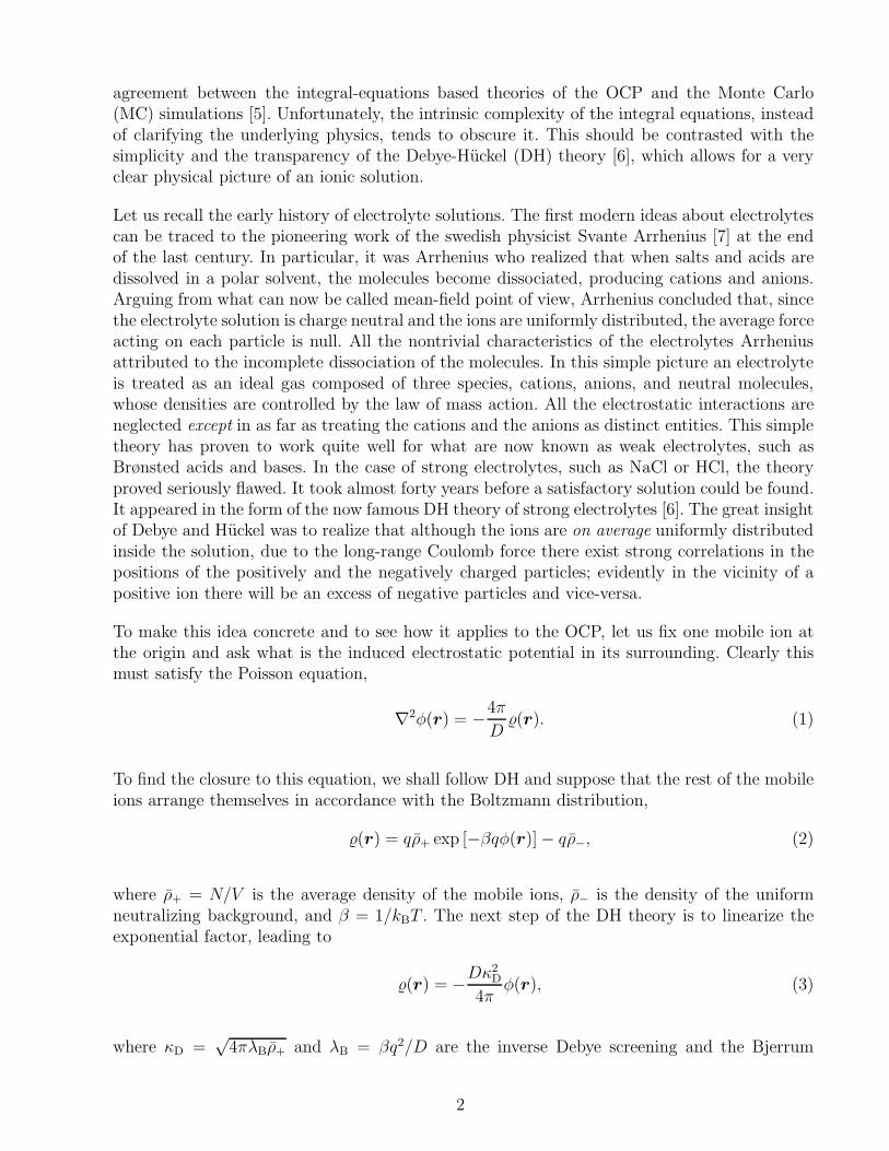
We see that the structure factor satisfies exactly the charge-neutrality and the second-momentconditions, while the compressibility sum rule is satisfied only to order Γ9/2. This results from thefact that, in order to simplify the calculations, we have neglected the dependence of the cavitysize and shape on the imposed density variation (∆). Clearly, if this was taken into account,the theory would be completely internally self consistent. Nevertheless, even at this level ofapproximation, the lack of self consistency is quite small over the full range of relevant couplingconstants, as can be measured by the inverse compressibilities derived from the thermodynamic(χP ) and the structure factor (χS) routes, Eqs. (56) and (60), respectively; see Fig. (1). The fitof the MC data [14] leads to an inverse compressibility (χMC) which is between the two previousones.

12

0 40 80 120 160Γ

−60

−40

−20

0

β/ρ_

+χP

β/ρ_

+χS

β/ρ_

+χMC

Fig. 1. Comparison between the inverse compressibilities derived from the pressure, Eq. (56), solidline (β/ρ+χP ), and from the structure factor, Eq. (60), long-dashed line (β/ρ+χS). The dashed line(β/ρ+χMC) represents the fit of the MC data over the interval 1 ≤ Γ ≤ 160 [14].

Defining k ≡ kd = α√

3Γ, we have explicitly carried out the summation for the first six termsof the infinite series in Eq. (53). The results for the structure factor for various values of Γ,obtained without any fitting parameters, are plotted in Figs. (2) to (5). The agreement with theMC simulations [15] is quite encouraging. We should note, however, that for higher couplings,in the vicinity of the first peak, the series is slowly convergent. This is the reason why we didnot attempt to carry the calculations for Γ > 40.

4 Conclusions

We have presented the generalized Debye-Huckel theory of the one-component plasma. Thelinearity of the theory allows for explicit calculations of all the thermodynamic functions, aswell as the structure factor, which is expressed as an infinite series. The linearity also insures theinternal consistency of the theory. The agreement with the Monte Carlo simulations, obtainedwithout any fitting parameters, is quite good, suggesting that the existence of an effective cavitysurrounding each ion is theoretically justified.

Acknowledgements

This work has been supported by the Brazilian agencies CNPq (Conselho Nacional de Desen-volvimento Cientıfico e Tecnologico), CAPES (Coordenacao de Aperfeicoamento de Pessoal de

13

0 2 4 6 8 10k^

0.0

0.4

0.8

1.2

S(k)^

Γ=2

Fig. 2. Structure factor S(k) for Γ = 2. The solid line is our expression (53) calculated up to ℓ = 6,while the circles represent the MC data [15].

0 2 4 6 8 10k^

0.0

0.4

0.8

1.2

S(k)^

Γ=6

Fig. 3. Structure factor S(k) for Γ = 6. The solid line is our expression (53) calculated up to ℓ = 6,while the circles represent the MC data [15].

Nıvel Superior) and FAPERGS (Fundacao de Amparo a Pesquisa do Estado do Rio Grande doSul).

14

0 2 4 6 8 10k^

0.0

0.4

0.8

1.2

S(k)^

Γ=10

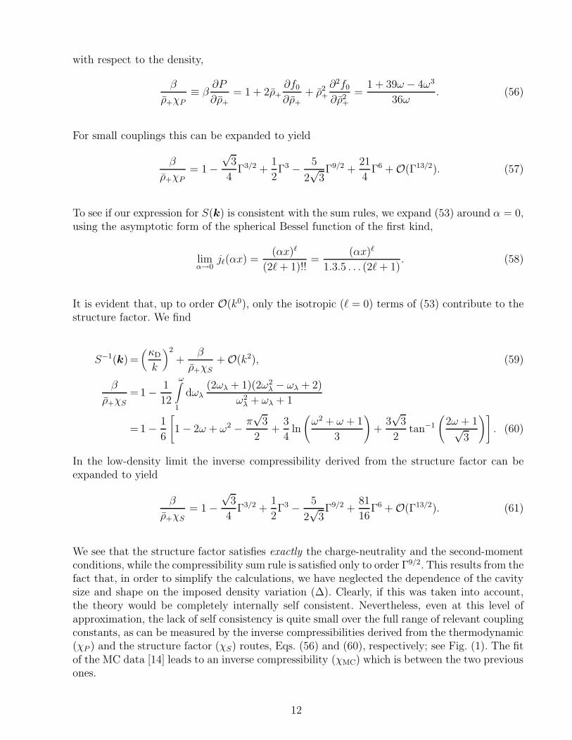
Fig. 4. Structure factor S(k) for Γ = 10. The solid line is our expression (53) calculated up to ℓ = 6,while the circles represent the MC data [15].

0 2 4 6 8 10k^

0.0

0.6

1.2

1.8

S(k)^

Γ=40

Fig. 5. Structure factor S(k) for Γ = 40. The solid lines are our expression (53) with the ℓ = 0, 1, 2, . . .up to the ℓ = 6 terms included in the sum (from top to bottom). The circles represent the MC data[15]. We note that for higher values of Γ, more and more terms will need to be included in order toachieve convergence in the vicinity of the first peak.

A Some useful integrals

In this appendix we present some integrals which appear along the text. We introduce theKronecker delta,

δk0 =1

V(2π)3δ3(k), (A.1)

15

where V = (2π)3δ3(0) is the volume of the system and δ3(k) is the three-dimensional Diracdelta function,

δ3(k) ≡(

1

2π

)3 ∫

d3r′ exp (ik · r′) . (A.2)

From the definition (A.2) of the three-dimensional Dirac delta function, it follows directly

∫

d3r′ cos k · r′ =1

2

∫

d3r′ [exp (ik · r′) + exp (−ik · r′)]

=1

2(2π)3

[

δ3(k) + δ3(−k)]

= (2π)3δ3(k) = V δk0, (A.3)∫

d3r′ cos2 k · r′ =1

2

∫

d3r′ (1 + cos 2k · r′) =1

2

[

V + (2π)3δ3(2k)]

=V

2(1 + δk0) . (A.4)

A simple generalization of (A.4) leads to

∫

d3r′ cos2(

k · r′ + ℓπ

2

)

=V

2

[

1 + (−1)ℓδk0

]

, (A.5)

where ℓ is an integer.

Expressing 1/r as the inverse Fourier transform

1

r=

1

2π2

∫

d3k1

k2exp (−ik · r) , (A.6)

we have

∫

d3r d3r′ cos k · r cos k · r′

|r − r′| =1

4π2

∫

d3r d3r′ d3q1

q2exp [−iq · (r − r′)]

× [cos k · (r + r′) + cos k · (r − r′)]

=1

8π2

∫

d3r d3r′ d3q1

q2

∑

α1=±

exp [i (α1k − q) · r]

×∑

α2=±

exp [i (α2k + q) · r′]

=1

2(2π)4

∫

d3q1

q2

∑

α1,α2=±

δ3(α1k − q) δ3(α2k + q)

=(2π)4

k2

[

δ3(0) +1

2δ3(2k) +

1

2δ3(−2k)

]

=2πV

k2(1 + δk0) . (A.7)

16

B Variation of the free-energy density

In this appendix we obtain the variation of the reduced free-energy density, δf = βδF/V , upto quadratic order in the perturbation parameter ∆.

The Helmholtz free energy F is written as a functional of the mobile-ion density ρ+(r). Thevariation δF is obtained using the functional Taylor series,

βδF [ρ+(r)] = βF [ρ+(r)] − βF [ρ+]

=∫

d3r′ βδF

δρ+(r′)

∣

∣

∣

∣

∣

ρ+(r)=ρ+

δρ+(r′)

+1

2

∫

d3r′ d3r′′ βδ2F

δρ+(r′) δρ+(r′′)

∣

∣

∣

∣

∣

ρ+(r)=ρ+

δρ+(r′) δρ+(r′′). (B.1)

The linear term can be written as

βδF (1) [ρ+(r)] =∫

d3r′ βδF

δρ+(r′)

∣

∣

∣

∣

∣

ρ+(r)=ρ+

δρ+(r′) =∫

d3r′ βµ(r′) δρ+(r′), (B.2)

where µ(r) is the chemical potential at the position r,

µ(r) ≡ δF

δρ+(r)

∣

∣

∣

∣

∣

ρ+(r)=ρ+

. (B.3)

However, at the thermodynamical equilibrium, the chemical potential of the system is constantand is independent of position,

µ(r) = µ, ∀r. (B.4)

Using the imposed variation (7) of the mobile-ion density,

δρ+(r) = ρ+∆ cos k · r =1

2ρ+∆ [exp (ik · r) + exp (−ik · r)] , (B.5)

the linear term can be expressed as

βδF (1) [ρ+(r)] = βµρ+∆∫

d3r′ cos k · r′ = βµρ+V∆δk0. (B.6)

The quadratic term,

17

βδF (2) [ρ+(r)]=1

2

∫

d3r′ d3r′′ βδ2F

δρ+(r′) δρ+(r′′)

∣

∣

∣

∣

∣

ρ+(r)=ρ+

δρ+(r′) δρ+(r′′)

=1

2

∫

d3r′ d3r′′

[

δ (r′ − r′′)

ρ+

− C++ (r′ − r′′)

]

δρ+(r′) δρ+(r′′), (B.7)

can be split into two parts, the ideal-gas contribution,

βδF(2)ideal [ρ+(r)] =

1

2ρ+

∫

d3r′ d3r′′ δ(r′ − r′′) δρ+(r′) δρ+(r′′), (B.8)

and the electrostatic contribution,

βδF(2)elect [ρ+(r)] = −1

2

∫

d3r′ d3r′′C++ (r′ − r′′) δρ+(r′) δρ+(r′′), (B.9)

where C++ (r′ − r′′) is the direct correlation function.

Using (A.4) and (B.5), the ideal-gas contribution can be straightforwardly obtained,

βδF(2)ideal [ρ+(r)] =

1

2ρ+

∫

d3r′ [δρ+(r′)]2

=1

2ρ+∆2

∫

d3r′ cos2 k · r′

=V

4ρ+∆2 (1 + δk0) . (B.10)

To evaluate the electrostatic contribution we use (B.5), and express C++ (r′ − r′′) as the inverseFourier transform

C++(r) =(

1

2π

)3 ∫

d3k C++(k) exp (−ik · r) , (B.11)

leading to

βδF(2)elect [ρ+(r)] =−1

8ρ2

+∆2(

1

2π

)3 ∫

d3r′ d3r′′ d3q C++(q)

×∑

α1=±

exp [i (α1k − q) · r′]∑

α2=±

exp [i (α2k + q) · r′′]

=−1

8ρ2

+∆2 (2π)3∫

d3q C++(q)∑

α1,α2=±

δ3(α1k − q) δ3(α2k + q)

=−1

8ρ2

+∆2 (2π)3{

C++(k)[

δ3(0) + δ3(2k)]

+ C++(−k)[

δ3(0) + δ3(−2k)]}

=−V4C++(k)ρ2

+∆2 (1 + δk0) , (B.12)

where we have used the symmetry of the direct correlation function, C++(k) = C++(−k).

18

Combining all the pieces, the variation of the reduced free-energy density can be written as

δf [ρ+(r)]=β

VδF (1) [ρ+(r)] +

β

VδF

(2)ideal [ρ+(r)] +

β

VδF

(2)elect [ρ+(r)]

= βµρ+∆δk0 +1

4

[

1 − ρ+C++(k)]

ρ+∆2 (1 + δk0)

= βµρ+∆δk0 +1

4S−1(k)ρ+∆2 (1 + δk0) , (B.13)

where S(k) is the structure factor. Note that the linear contribution to the variation has a Kro-necker delta (δk0) factor, which expresses the translational invariance (B.3) of the equilibriumchemical potential µ of the system.

C Green’s function associated with the induced potential

In this appendix we obtain the Green’s function associated with the differential equation sat-isfied by the induced potential φ(r, r′).

The Green’s function G (R,R′) associated with (31), where R = r − r′, satisfies the homoge-neous equation [9]

[

∇2R − κ2

DΘ (|R| − h)]

G (R,R′) =−4πδ3(R − R′)

=−4π

R2δ(R− R′) δ(cos θ − cos θ′) δ(ϕ− ϕ′), (C.1)

with Θ(ξ) the Heaviside step function.

The general solution of (C.1) can be written as [9]

G (R,R′) = κD

∞∑

ℓ=0

Gℓ (κDR, κDR′)Pℓ

(

R · R′

RR′

)

, (C.2)

where Pℓ(ξ) denotes a Legendre polynomial.

Replacing (C.2) into (C.1), multiplying both sides by Pℓ′

(

R · R′

RR′

)

and integrating over the

angular coordinates θ and ϕ, we obtain the equation satisfied by the radial functions Gℓ (s, s′),

[

d2

ds2+

2

s

d

ds− Θ (s− x) − ℓ(ℓ+ 1)

s2

]

Gℓ (s, s′) = − 1

s2(2ℓ+ 1) δ(s− s′), (C.3)

where we have introduced the adimensional variables s = κDR, s′ = κDR′ and x = κDh. To

19

obtain (C.3) we have used the property of the Dirac delta function,

δ(κDR− κDR′) =

1

κD

δ(R− R′), (C.4)

the addition theorem for the Legendre polynomials,

Pℓ

(

R · R′

RR′

)

=Pℓ [cos θ cos θ′ + sin θ sin θ′ cos(ϕ− ϕ′)] (C.5)

=Pℓ(cos θ)Pℓ(cos θ′) + 2ℓ∑

m=1

(ℓ−m)!

(ℓ+m)!Pm

ℓ (cos θ)Pmℓ (cos θ′) cosm(ϕ− ϕ′),

and their orthogonality,

1∫

−1

d(cos θ)Pℓ(cos θ)Pℓ′(cos θ) =2

2ℓ+ 1δℓℓ′. (C.6)

The solutions of (C.3) that are finite for s→ 0 and vanish as s→ ∞ can be written as

Gℓ (s, s′) =

A11sℓ, for 0 < s < s′ < x,

A12sℓ + A13s

−(ℓ+1), for 0 < s′ < s < x,

A21sℓ, for 0 < s < x < s′,

A22kℓ(s), for 0 < s′ < x < s,

A31kℓ(s), for 0 < x < s′ < s,

A32iℓ(s) + A33kℓ(s), for 0 < x < s < s′,

(C.7)

where the coefficients {Amn} are functions of x and s′ to be determined by the boundaryconditions; iℓ(s) and kℓ(s) are the modified spherical Bessel functions of the first and the thirdkinds [16], respectively,

iℓ(s)=

√

π

2sIℓ+1/2(s), (C.8)

kℓ(s)=

√

2

πsKℓ+1/2(s). (C.9)

Using the symmetry property of the Green’s function [17], we can rewrite Eqs. (C.7) as

G(1)ℓ (s, s′) =A1s

ℓs′ℓ +B1sℓ

<

sℓ+1>

, for 0 < s, s′ < x, (C.10)

20

G(2)ℓ (s, s′) =A2s

ℓ<kℓ(s>), for 0 < s< < x < s>, (C.11)

G(3)ℓ (s, s′) =A3kℓ(s)kℓ(s

′) +B3iℓ(s<)kℓ(s>), for 0 < x < s, s′, (C.12)

where s< = min(s, s′), s> = max(s, s′), and the coefficients {An, Bn} depend now only on thesize of the exclusion hole x.

The coefficients {Bn}, n = 1, 3, are obtained by imposing the discontinuity of the derivative ofGℓ(s, s

′) associated with the Dirac delta function,

d

ds

[

sG(n)ℓ (s, s′)

]

s=s′+ǫ− d

ds

[

sG(n)ℓ (s, s′)

]

s=s′−ǫ= −2ℓ+ 1

s′, (C.13)

where ǫ is a positive infinitesimal. Using the Wronskian of the modified spherical Bessel functions[16],

W [kℓ(s), iℓ(s)] = kℓ(s)i′ℓ(s) − iℓ(s)k

′ℓ(s) =

1

s2, (C.14)

this leads to

B1 = 1, (C.15)

B3 = 2ℓ+ 1. (C.16)

The coefficients {An}, n = 1, 2, 3, are obtained by imposing the continuity of Gℓ(s, s′) and of

its derivative across the spherical surface at s = s′ = x,

G(1)ℓ (s, s′)

∣

∣

∣

s=s′=x= G

(2)ℓ (s, s′)

∣

∣

∣

s=s′=x= G

(3)ℓ (s, s′)

∣

∣

∣

s=s′=x, (C.17)

d

dsG

(1)ℓ (s, s′)

∣

∣

∣

∣

∣

s=s′+ǫ=x

=d

dsG

(2)ℓ (s, s′)

∣

∣

∣

∣

∣

s=s′+ǫ=x

, (C.18)

and using the following relations of the modified spherical Bessel functions [16] to express iℓ(x),kℓ(x) and k′ℓ(x) in terms of iℓ±1(x) and kℓ±1(x),

1

x2= iℓ+1(x)kℓ(x) + kℓ+1(x)iℓ(x), (C.19)

(2ℓ+ 1) kℓ(x) = xkℓ+1(x) − xkℓ−1(x), (C.20)

− (2ℓ+ 1) k′ℓ(x) = ℓkℓ−1(x) + (ℓ+ 1) kℓ+1(x), (C.21)

which yield

A1 =− kℓ−1(x)

x2ℓ+1kℓ+1(x), (C.22)

21

A2 =2ℓ+ 1

xℓ+2kℓ+1(x), (C.23)

A3 =(2ℓ+ 1)iℓ+1(x)

kℓ+1(x). (C.24)

Therefore, the Green’s function G (R,R′) is given by the expansion (C.2), with the radialfunctions Gℓ (s, s′) defined by [9]

G(1)ℓ (s, s′) =

sℓ<

sℓ+1>

− sℓs′ℓkℓ−1(x)

x2ℓ+1kℓ+1(x), for 0 < s, s′ < x, (C.25)

G(2)ℓ (s, s′) = (2ℓ+ 1)

sℓ<kℓ(s>)

xℓ+2kℓ+1(x), for 0 < s< < x < s>, (C.26)

G(3)ℓ (s, s′) = (2ℓ+ 1)

[

iℓ+1(x)

kℓ+1(x)kℓ(s)kℓ(s

′) + iℓ(s<)kℓ(s>)

]

, for 0 < x < s, s′. (C.27)

D The perturbative solution of the induced potential

In this appendix we obtain the induced potential φ(r, r′) recursively, up to order ∆2, at thecenter of the exclusion hole, |r − r′| = 0.

Let us obtain the induced potential outside the exclusion hole, |r−r′| ≥ h, which we will denoteby φ>(r, r′). Clearly, this potential is produced by the charge distribution inside and outsidethe cavity. Let us first calculate the contribution to the potential arising from the charge inside

the hole, φ(<)> (r, r′). Since our final goal is to calculate the potential at the center of the cavity

to order ∆2, it is sufficient to calculate the induced potential outside the hole to order ∆, seeEq. (33). Using the Green’s function G (R,R′) derived in appendix C, where R = r − r′, wefind to first order in ∆,

φ(<)> (r, r′)= φ

(<)> (R + r′, r′) =

1

D

∫

|R′|≤h

d3R′ (R′)G (R,R′)

=qκD

D

∫

|R′|≤h

d3R′{

δ3(R′) − ρ+ [1 + ∆ cos k · (R′ + r′)]}

×∞∑

ℓ=0

Pℓ

(

R · R′

RR′

)

=1

βq

(

λBκD − 1

3x3)

k0(κDR)

x2k1(x)− qρ+κD

D∆ Re

[

exp (ik · r′)∞∑

ℓ=0

(2ℓ+ 1)

× kℓ(κDR)

xℓ+2kℓ+1(x)

∫

|R′|≤h

d3R′ (κDR′)

ℓexp (ik · R′)Pℓ

(

R · R′

RR′

)

, (D.1)

22

recalling that x = κDh. The first term of (D.1) can be simplified using the identities

k1(x) = (1 + x)e−x

x2, (D.2)

λBκD =1

3

[

(1 + x)3 − 1]

= x (1 + x) +1

3x3. (D.3)

The relation (D.3) is the defining equation for the cavity size, x, Eq. (5). It is important toremember that it does not take into account the imposed variation in the ionic density, and asresult will be responsible for the violation of the compressibility sum rule.

To simplify the second term of (D.1), we note first that, without loss of generality, we canchoose the z axis along the k direction,

cos θ=k · RkR

, cos θ′ =k · R′

kR′, (D.4)

tanϕ=R · yR · x , tanϕ′ =

R′ · yR′ · x , (D.5)

so that the addition theorem for the Legendre polynomials can be written as

Pℓ

(

R · R′

RR′

)

=Pℓ [cos θ cos θ′ + sin θ sin θ′ cos(ϕ− ϕ′)] (D.6)

=Pℓ(cos θ)Pℓ(cos θ′) + 2ℓ∑

m=1

(ℓ−m)!

(ℓ+m)!Pm

ℓ (cos θ)Pmℓ (cos θ′) cosm(ϕ− ϕ′).

Performing the integrations over the azimuthal angle ϕ′, only the m = 0 terms survive,

φ(<)> (r, r′)=

1

βqxexk0(κDR) − κ3

D

βq∆ Re

[

exp (ik · r′)∞∑

ℓ=0

(2ℓ+ 1)kℓ(κDR)

xℓ+2kℓ+1(x)

× Pℓ(cos θ)

h∫

0

dR′R′2 (κDR′)

ℓ1∫

−1

d(cos θ′) exp (ikR′ cos θ′)Pℓ(cos θ′)

. (D.7)

To proceed, we use the plane-wave expansion,

exp (ikR′ cos θ′) =∞∑

ℓ=0

(2ℓ+ 1) iℓjℓ(kR′)Pℓ(cos θ′), (D.8)

where jℓ(ξ) is the spherical Bessel function of the first kind,

jℓ(ξ) =

√

π

2ξJℓ+1/2(ξ). (D.9)

23

The integrations over the polar angle θ′ and over the radial coordinate R′ can be performedusing the orthogonality of the Legendre polynomials,

1∫

−1

d(cos θ′)Pℓ(cos θ′)Pℓ′(cos θ′) =2

2ℓ+ 1δℓℓ′, (D.10)

and the recursion relation for the spherical Bessel function of the first kind,

d

dξ

[

ξℓ+2jℓ+1(ξ)]

= ξℓ+2jℓ(ξ), (D.11)

which yields

φ(<)> (r, r′)= φ

(<)> (R + r′, r′) =

1

βqxexk0(κDR) − 1

αβq∆

∞∑

ℓ=0

(2ℓ+ 1) cos(

k · r′ + ℓπ

2

)

× jℓ+1(αx)

kℓ+1(x)kℓ(κDR)Pℓ(cos θ), (D.12)

where α = k/κD.

Substituting φ(<)> (r, r′) into the expression for the charge density outside the exclusion hole,

Eq. (33), we can now calculate the contribution to the potential outside the exclusion hole

arising from the external charge, φ(>)> (r, r′). To order ∆ we find

φ(>)> (r, r′)= φ

(>)> (R + r′, r′) =

1

D

∫

|R′|≥h

d3R′ (R′)G (R,R′)

=−κ3D

4π∆

∫

|R′|≥h

d3R′ φ(<)> (R′ + r′, r′) cos k · (R′ + r′)

×∞∑

ℓ=0

G(3)ℓ (κDR, κDR

′)Pℓ

(

R · R′

RR′

)

=− 1

βqxex∆

∞∑

ℓ=0

(2ℓ+ 1) cos(

k · r′ + ℓπ

2

)

Ξℓ(κDR,α)Pℓ(cos θ), (D.13)

where the function Ξℓ(s, α) is defined by

Ξℓ(s, α)=

∞∫

x

ds′ s′2 k0(s′)G

(3)ℓ (s, s′)

2ℓ+ 1jℓ(αs

′)

=iℓ+1(x)

kℓ+1(x)kℓ(s)

∞∫

x

dξ ξ2k0(ξ)kℓ(ξ)jℓ(αξ) + kℓ(s)

s∫

x

dξ ξ2k0(ξ)iℓ(ξ)jℓ(αξ)

24

+ iℓ(s)

∞∫

s

dξ ξ2k0(ξ)kℓ(ξ)jℓ(αξ). (D.14)

We are now able to find the induced potential inside the exclusion hole, |r − r′| ≤ h, up toorder ∆2,

φ<(r, r′)= φ<(R + r′, r′) =1

D

∫

d3R′ (R′)G (R,R′)

=qκD

D

∫

|R′|≤h

d3R′{

δ3(R′) − ρ+ [1 + ∆ cos k · (R′ + r′)]}

×∞∑

ℓ=0

G(1)ℓ (κDR, κDR

′)Pℓ

(

R · R′

RR′

)

− κ3D

4π∆

∫

|R′|≥h

d3R′ φ>(R′ + r′, r′)

× cos k · (R′ + r′)∞∑

ℓ=0

G(2)ℓ (κDR, κDR

′)Pℓ

(

R · R′

RR′

)

, (D.15)

where the induced potential outside the exclusion hole, up to order ∆, is given by

φ>(r, r′) = φ(<)> (r, r′) + φ

(>)> (r, r′). (D.16)

Since we need just the mean induced electrostatic potential ψ(r′) felt by the positive ion fixed atr′, that is, at the center of the exclusion hole, R = 0, and recalling that Gℓ(κDR = 0, κDR

′) =0, ∀ℓ > 0, only the isotropic (ℓ = 0) terms of (D.15) contribute,

ψ(r′) = limR→0

[

φ<(R + r′, r′) − q

DR

]

= limR→0

qκD

D

∫

|R′|≤h

d3R′G(1)0 (κDR, κDR

′) δ3(R′) − q

DR

− qρ+κD

D

∫

|R′|≤h

d3R′G(1)0 (0, κDR

′) [1 + ∆ cosk · (R′ + r′)]

− κ3D

4π∆

∫

|R′|≥h

d3R′G(2)0 (0, κDR

′) φ>(R′ + r′, r′) cosk · (R′ + r′)

= limR→0

[

qκD

DG

(1)0 (κDR, 0) − q

DR

]

− κ3D

βq

h∫

0

dR′R′2G(1)0 (0, κDR

′)

− κ3D

βq∆ cos k · r′

h∫

0

dR′R′2G(1)0 (0, κDR

′)j0(kR′)

− κ3D

4π

1

x2k1(x)∆

∫

|R′|≥h

d3R′ k0(κDR′) φ>(R′ + r′, r′) cos k · (R′ + r′) . (D.17)

25

Using the explicit form of G(1)0 (s, s′) and φ>(r, r′), and performing the angular integrations, we

obtain

βqψ(r′)=−λBκDk−1(x)

xk1(x)−

x∫

0

ds s2

[

1

s− k−1(x)

xk1(x)

]

− ∆ cos k · r′

x∫

0

ds s2

[

1

s− k−1(x)

xk1(x)

]

j0(αs) +xe2x

1 + x

∞∫

x

ds s2k20(s)j0(αs)

+ex

α (1 + x)∆2

∞∑

ℓ=0

(2ℓ+ 1) cos2(

k · r′ + ℓπ

2

)

jℓ+1(αx)

kℓ+1(x)

∞∫

x

ds s2k0(s)kℓ(s)jℓ(αs)

+xe2x

1 + x∆2

∞∑

ℓ=0

(2ℓ+ 1) cos2(

k · r′ + ℓπ

2

)

∞∫

x

ds s2k0(s)Ξℓ(s, α)jℓ(αs). (D.18)

The first terms of (D.18) can be simplified using (D.2) and (D.3), supplemented by the identities

k0(x) =e−x

x, (D.19)

k−1(x)

k1(x)=k1(x) − k0(x)/x

k1(x)=

x

1 + x, (D.20)

j0(ξ)=sin ξ

ξ. (D.21)

Furthermore, expressing iℓ(ξ) in terms of kℓ(ξ) using the relation [16]

iℓ(ξ) = −1

2

[

kℓ(−ξ) + (−1)ℓkℓ(ξ)]

, (D.22)

and defining the ℓ-th grade polynomial gℓ(ξ) associated with the modified spherical Besselfunction of the third kind kℓ(ξ) by the identity [16]

gℓ(ξ) ≡ eξξℓ+1kℓ(ξ) =ℓ∑

m=0

Γ(ℓ+m+ 1)

2mm! Γ(ℓ−m+ 1)ξℓ−m =

ℓ∑

m=0

(2m)!

2mm!

(

ℓ+m

2m

)

ξℓ−m, (D.23)

where Γ(m) = (m− 1)! is the Euler gamma function, it is possible to express the last integralof (D.18), which is two-dimensional, in terms of one-dimensional quadratures,

∞∫

x

ds s2k0(s)Ξℓ(s, α)jℓ(αs)= e−2x(−1)ℓ+1

{

1

2

gℓ+1(−x)gℓ+1(x)

[

I+ℓ (x, α)

]2

+ I+ℓ (x, α)I−

ℓ (x, α) − I0ℓ (x, α)

}

, (D.24)

where {Iνℓ }, ν = ±, 0, are the one-dimensional integrals

26

I−ℓ (s, α)=

s∫

0

dξ ξ−ℓgℓ(−ξ)jℓ(αξ), (D.25)

I0ℓ (x, α)=

∞∫

x

ds s−ℓgℓ(s)jℓ(αs)I−ℓ (s, α) exp [2(x− s)] , (D.26)

I+ℓ (x, α)=

∞∫

x

ds s−ℓgℓ(s)jℓ(αs) exp [2(x− s)] . (D.27)

We stress that the functions {I0ℓ (x, α)} represent one-dimensional quadratures, since the inte-

grals {I−ℓ (s, α)} can be expressed in explicit form, for all values of ℓ, in terms of trigonometric

functions and of the sine integral,

Si (t) =

t∫

0

dξsin ξ

ξ. (D.28)

To illustrate, we give the three first integrals:

I−0 (s, α)=

Si (αs)

α, (D.29)

I−1 (s, α)=− 1

α+

cosαs

2αs+(

1

α2s− 1

2α2s2

)

sinαs+1

2Si (αs), (D.30)

I−2 (s, α)=−1 +

(

3

2α2s− 3

α2s2+

9

4α2s3+

3

8s

)

cosαs

+(

− 3

2α3s2+

3

α3s3− 9

4α3s4+

3

8αs2

)

sinαs+(

1

2α+

3α

8

)

Si (αs). (D.31)

Therefore, the final form for the mean induced electrostatic potential at the center of theexclusion hole (in unities of βq) reads

βqψ(r′)=−1

2x(x+ 2) − ∆ cos k · r′

[

1

α2− sinαx

α3(1 + x)− cosαx

α2(1 + x)+

x

1 + xI+

0 (x, α)

]

+1

α(1 + x)∆2

∞∑

ℓ=0

(2ℓ+ 1) cos2(

k · r′ + ℓπ

2

)

xℓ+2jℓ+1(αx)

gℓ+1(x)I+

ℓ (x, α)

+x

1 + x∆2

∞∑

ℓ=0

(−1)ℓ+1 (2ℓ+ 1) cos2(

k · r′ + ℓπ

2

)

×{

1

2

gℓ+1(−x)gℓ+1(x)

[

I+ℓ (x, α)

]2+ I+

ℓ (x, α)I−ℓ (x, α) − I0

ℓ (x, α)

}

. (D.32)

References

27

[1] E. E. Salpeter, Ann. Physics 5 (1958) 183; R. Abe, Progr. Theor. Phys. 22 (1959) 213.

[2] M. Baus, J.-P. Hansen, Phys. Rep. 59 (1980) 1.

[3] S. Alexander, P. M. Chaikin, P. Grant, G. J. Morales, P. Pincus, D. Hone, J. Chem. Phys. 80

(1984) 5776; K. Kremer, M. O. Robbins, G. S. Grest, Phys. Rev. Lett. 57 (1986) 2694; Y. Levin,M. C. Barbosa, M. N. Tamashiro, Europhys. Lett. 41 (1998) 123; M. N. Tamashiro, Y. Levin, M.C. Barbosa, Physica A 258 (1998) 341.

[4] F. J. Rogers, H. E. DeWitt, eds., Strongly Coupled Plasmas, Plenum Press, New York, 1987; G.Zerah, J. Clerouin, E. L. Pollock, Phys. Rev. Lett. 69 (1992) 446.

[5] K.-C. Ng, J. Chem. Phys. 61 (1974) 2680; Y. Rosenfeld, Phys. Rev. E 54 (1996) 2827.

[6] P. Debye, E. Huckel, Phys. Z. 24 (1923) 185; 305; D. A. McQuarrie, Statistical Mechanics, chapter15, Harper-Collins, New York, 1976.

[7] S. Arrhenius, Z. Phys. Chem. 1 (1887) 631.

[8] S. Nordholm, Chem. Phys. Lett. 105 (1984) 302; R. Penfold, S. Nordholm, B. Jonsson, C. E.Woodward, J. Chem. Phys. 92 (1990) 1915.

[9] B. P. Lee, M. E. Fisher, Phys. Rev. Lett. 76 (1996) 2906; Europhys. Lett. 39 (1997) 611.

[10] F. H. Stillinger, R. Lovett, J. Chem. Phys. 48 (1968) 3858; J. Chem. Phys. 49 (1968) 1991.

[11] J. G. Kirkwood, Chem. Rev. 19 (1936) 275.

[12] One should mention, however, integral equations such as the generalized mean-sphericalapproximation (GMSA) [G. Stell, S. F. Sun, J. Chem. Phys. 63 (1975) 5333] and the self-consistentOrnstein-Zernike approximation (SCOZA) [J. S. Høye, G. Stell, Mol. Phys. 52 (1984) 1071], whichwere constructed to explicitly enforce the self consistency.

[13] M. E. Fisher, Y. Levin, Phys. Rev. Lett. 71 (1993) 3826; Y. Levin, X.-J. Li, M. E. Fisher, Phys.Rev. Lett. 73 (1994) 2716; Y. Levin, M. E. Fisher, Physica A 225 (1996) 164.

[14] H. E. DeWitt, Phys Rev. A 14 (1976) 1290.

[15] S. Galam, J.-P. Hansen, Phys. Rev. A 14 (1976) 816.

[16] A. Erdelyi, W. Magnus, F. Oberhettinger, F. G. Tricomi, eds., Higher Transcendental Functions,Bateman Manuscript Project, vol. II, chapter 7, McGraw-Hill, New York, 1953; M. Abramowitz, I.A. Stegun, eds., Handbook of Mathematical Functions with Formulas, Graphs, and MathematicalTables, National Bureau of Standards, Applied Mathematics Series 55, chapter 10, U.S.Government Printing Office, Washington D.C., 1964.

[17] J. D. Jackson, Classical Electrodynamics, second edition, sect. 3.9, John Wiley & Sons, New York,1975.

28