THE OHIO STATE UNIVERSITY- DEPARTMENT OF AEROSPACE/ MECHANICAL ENGINEERING€¦ · · 2014-04-11THE OHIO STATE UNIVERSITY- DEPARTMENT OF AEROSPACE/ MECHANICAL ENGINEERING ... An

THE OHIO STATE UNIVERSITY- DEPARTMENT OF AEROSPACE/ MECHANICAL ENGINEERING

Simulating the Effect of Plasma Actuators on the

Three-Dimensionality of the Wake of a Cylinder in a

Crossflow Undergraduate Research Thesis

By

Cory Stack

Presented in partial fulfillment of the requirements for Bachelor of Science in Aerospace

Engineering with Research Distinction for May 2014

Thesis Committee:

Dr. Datta Gaitonde, Advisor

Dr. Carl Hartsfield

Dr. Mei Zhaung

1

2

Copyright by

Cory Stack

2014

3

Abstract

Bluff body flow control techniques are essential when assessing the impact of an

aerodynamic load to a structural response or aerodynamic efficiency. Plasma actuators

are a unique active flow control technique due to their fast response time, lack of

moving parts, low mass, purely electric nature and simple integration into many

geometries. These actuators add momentum to the boundary layer from ionized plasma

acting as a body force on the neutral air, resulting in different flow structures. In this

research, the cylinder is in a flow regime where von Kármán and Kelvin-Helmholtz

shedding occurs; resulting in transient pressure variations which induce vibrations on

the cylinder, possibly triggering resonance and leading to structural failure. Plasma

actuators have proven effective in reducing or virtually eliminating shedding from

occurring. Previous fluid dynamic simulations have used actuators across the entire span

of the cylinder, resulting in a two dimensional impact on the wake. This research uses

staggered actuators across the span of the cylinder, so certain regions will experience a

velocity change, while other regions will not; a three dimensional wake effect. All

simulations use a momentum source coupled into the momentum equation of the

Navier-Stokes equations with a pressure-based laminar solver, SIMPLE pressure-velocity

coupling, and a time step of .001s. The ability to simulate the three dimensionality effect

of the plasma actuators helps provide insight if staggered actuators produce a similar

effect as spanwise actuators. Since simulations are cost and relatively time effective, the

model can be extended to other scenarios to learn if plasma actuators can provide a

similar response as they do for a cylinder in a crossflow.

4

Dedication

This paper is dedicated to my parents.

5

Acknowledgements

I would like to thank Dr. Gaitonde for his advice during my research and the

opportunities he has presented to me. I would also like to thank Dr. Hartsfield and Dr.

Zhaung for their aid as committee members.

6

Vita

2010 to present……………………………………………………………………………. B.S. Mechanical and

Aerospace Engineering, The

Ohio State University

7

Table of Contents

Abstract……………………………..………………………………………………………………………………3

Dedication………………………………………………………………………………………………………….4

Acknowledgements……………………………………………………………………………………………5

Vita…………………………………………………………………………………………………………………….6

List of Figures……………………………………………………………………………………………………..8

List of Tables…………………………………………………………………………………………….…….…10

1. Introduction ………………………………………………………………….…………………………....……11

2. Background………………………………………………………………………………………….…….………12

2.1 Fluid Mechanics …………………………………………………………………………..…….…12

2.2 Plasma Discharge Physics…………………………………………………………..………...13

2.3 Parameters Affecting the Plasma Discharge………………………………….…..….14

2.4 Current Modeling Techniques………………………………………………………..………15

3. Solver Settings……………………………………………………………………………………………………16

3.1 Plasma Modeling Technique…………………………………………………….……………16

3.2 Governing Equations………………………………………………………………………..…….16

3.3 Assumptions of the Model……………………………………………………….…….……..17

3.4 Universal Solver Settings…………………………………………………………………….…18

4. Two Dimensional Results………………………………………………………………………...………..18

4.1 Meshes Used……………………………………………………………………………….………..18

4.2 Solver Settings……………………………………………………………………………….……..19

4.3 Results without Plasma Actuation………………………………….……………………..20

4.4 Results with Plasma Actuation…………………………………………………..………….25

4.5 Mesh Dependency Results.………………………………………..……………..…………..31

4.6 One Sided Source……………………………………………………………...…………………..35

5. Three Dimensional Results……………………………………….……………………………………….37

5.1 Mesh…………………………………………………………………….………………………………37

5.2 Solver Settings………………………………………………………………………………………39

5.3 Results without Plasma Actuation………………….……………………………………..39

5.4 Results with Varying Strength of Plasma Actuation…………….…….………….40

5.5 Transient Results of a given Plasma Actuation Strength……………………….42

6. Conclusion………………………………………………………………………………..……………………...53

7. Future Work……………………………………………………………………………………………………..54

Appendix A: Sample Code………………………………………………………………………………………55

8

List of Figures

Figure 1: Schematic of a DBD plasma actuator………………………………….………………………..11

Figure 2: 2D Fine Mesh……………………………………………………………………………….………………19

Figure 3: 2D Coarse Mesh…………………………………………………………………………....…………….19

Figure 4: Baseline Lift Coefficient for Fine Mesh…………………………………………..…..………..20

Figure 5: Velocity Magnitude Contours of Baseline Case with Fine Mesh…….…...……..…21

Figure 6: Vorticity Magnitude Contours of Baseline Case with Fine Mesh………….……….23

Figure 7: Pressure Coefficient Contours of Baseline Case with Fine Mesh……….………….24

Figure 8: Vorticity Contours for a Source Strength of 100,000

…………………….…………26

Figure 9: Lift Coefficient for a Source Strength of 100,000

…………………....…….………...26


……………………..……….27


……………………………...…….28

Figure 12: Pressure Coefficient Contours for a Source Strength of 250,000

…………….29


………………………………30


…………………………………….30

Figure 15: Baseline Lift Coefficients for Fine Mesh and Coarse Mesh…………………………..32

Figure 16: Vorticity Contours on Coarse Mesh for a Source Strength of 500,000

…….32

Figure 17: Lift Coefficient on Coarse Mesh for a Source Strength of 500,000

…………..33


……...34


……...…….35


on Top of Cylinder...36

9


on Top Half of Cylinder..36

Figure 22: Three dimensional mesh……………………………………………………………………………..37

Figure 23: Three Dimensional Baseline Results…………………………………………………………….39

Figure 24: Three Dimensional Baseline Lift Coefficient…………………………………………………40

Figure 25: 3D Mesh Testing Velocity Magnitude Contours…………………………………………..41

Figure 26: Curve of 3D Mesh Source Strengths vs Maximum Velocity………………………….41

Figure 27: Lift Coefficient for 3D Case with Source Strength 175,000

………………………42

Figure 28: 90o Location on Cylinder Normal to X………………………………………………………….43

Figure 29: Edge of the Cylinder Normal to X………………………………………………………………...44

Figure 30: A Quarter of an Inch Past the Cylinder Normal to X……………………………………..46

Figure 31: A Half of an Inch Past the Cylinder Normal to X……………………………………………47

Figure 32: An Inch Past the Cylinder Normal to X…………………………………………………………48

Figure 33: An Inch and a Quarter in the Z-Direction Normal to Z…………………………………50

Figure 34: Combined Views of Fig. 29 and Fig.33…………………………………………………………51

Figure 35: Instantaneous Isosurfaces of Vorticity Colored by X-Velocity………………………52

10

List of Tables

Table 1: Two Dimensional Mesh Statistics…………………………………………………………………...18

Table 2: Statistics of Two Dimensional Momentum Source………………………………………….25

Table 3: Statistics of 3D Source Strength Testing………………………………………………………….41

11

1. Introduction

A body can be deemed bluff it has a profound cross section perpendicular to the

flow direction. Flow over a sphere, around a building, or a truck moving through air are

all considered bluff body flow. Behind these objects there is a region where the flow is

slowed, called the wake. Bluff bodies experience a large wake, leading to large pressure

drag. Under certain conditions, the wake of bluff bodies can shed von Kármán and

Kelvin-Helmholtz vortices. This shedding creates a periodic, unsteady force from

pressure variations in the wake which vibrate the body and can lead to resonance and

structural failure. To control vortex shedding, either passive or active flow control

methods can be used. Passive methods are fixed changes in a geometry driven by a

known condition (golf ball dimples, fairings, streaks, etc.) while active methods involve a

response to an existing condition (jet actuators, deployable fins, etc.).

Figure 1[1]: Schematic of a DBD plasma actuator

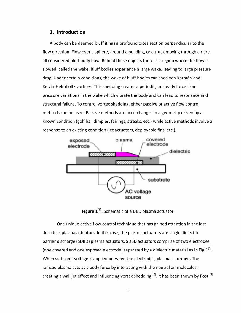
One unique active flow control technique that has gained attention in the last

decade is plasma actuators. In this case, the plasma actuators are single dielectric

barrier discharge (SDBD) plasma actuators. SDBD actuators comprise of two electrodes

(one covered and one exposed electrode) separated by a dielectric material as in Fig.1[1].

When sufficient voltage is applied between the electrodes, plasma is formed. The

ionized plasma acts as a body force by interacting with the neutral air molecules,

creating a wall jet effect and influencing vortex shedding [2]. It has been shown by Post [3]

12

that modifying the electrode arrangement can change the induced velocity to produce

not only wall jet, but also spanwise vortices or streamwise vortices. The uniqueness of a

SDBD separates itself from other flow active control techniques; it has no moving parts,

is purely electronic, with fast response time, low mass and can be adhered to nearly any

geometry without significant aerodynamic side-effects [4]. Some uses of SDBDs are on

landing gear of aircraft in effort to reduce vibrations on takeoff due to shedding [1], low

pressure turbine blade separation control [5], and for biomedical purposes, specifically

skin treatment [6].

The purpose of this research is to simulate the flow response to electrodes

staggered across the span of the cylinder, with some regions experiencing a different

velocity change than others; a three dimensional effect in the wake. Previous

computational fluid dynamics simulations of plasma actuators have been only in a two

dimensional domain where only spanwise vortices are formed. Within a three

dimensional wake, there are streamwise vortices as well as spanwise vortices that

increase mixing the wakes of the regions with and without actuation. All simulations are

completed in Ansys Fluent with steady actuation. Two dimensional simulations were

completed first to gain insight on the impact of a mesh and source strength to flow

response before completing three dimensional simulations.

2. Background

2.1 Fluid Mechanics

Using a cylinder to study and model flow control using plasma actuation is

convenient, as the fluid mechanics of a cylinder in a cross flow are well understood.

From the frontal stagnation point, the fluid accelerates under a favorable pressure

gradient. When the fluid reaches 90 degrees from the frontal stagnation location, the

pressure will reach a minimum and the velocity will reach a maximum. After this point

the flow faces an adverse pressure gradient and begins to decelerate. Once the fluid

experiences a velocity gradient such that

, the flow separates from the

surface. This location is the separation point, and is the result of the fluid near the

13

cylinder surface lacking sufficient momentum to overcome the adverse pressure

gradient [7]. The flow then detaches from the surface and a wake forms downstream of

the cylinder. In this regime, low pressure flow within the wake is comprised of von

Kármán and Kelvin-Helmholtz vortices due to shear layer roll up. Starting at the two

separation points, the flow will periodically alternate shedding parcels of fluid as time

lapses. As these fluid parcels are released the pressure distribution within the wake also

changes, resulting in induced vibrations from vortex shedding. These vortices are not

shed randomly; rather they follow the dimensionless parameter called the Strouhal

number (St). Mathematically,

, where f is the shedding frequency, D is the

cylinder diameter, and is the free stream velocity. For a more in-depth review of

vortex shedding features visit Asyikin [8]. Generally SDBDs are placed near the separation

point, giving the boundary layer additional momentum to overcome the adverse

pressure gradient while moving the flow separation location and possibly eliminating

vortex shedding.

2.2 Plasma Discharge Physics

As shown in Fig. 1[1], a SDBD plasma actuator consists of a single dielectric barrier

separating two electrodes. AC voltage is applied to generate an electric field between

the electrodes. When the magnitude of the electric field is large enough, it will cause a

Townsend discharge to occur followed by streamer formation [9]. Streamers are small

filament discharges that have lives on the order of nanoseconds, and efficiently transfer

electric charge from the exposed electrode to the plasma volume above the dielectric

due to their high electrical conductivity. For a sinusoidally driven SDBD, the temperature

of the plasma rises only slightly due to the added electrical energy being primarily used

to generate energetic electrons [4]. The electrostatic force renders this plasma volume

self-limiting due to attraction of the plasma from the buried electrode, and repulsion

from the exposed electrode (since the plasma carries same charge as exposed

electrode). Unless the magnitude of the applied voltage continuously increases, the

plasma discharge will terminate [1]. The character of the plasma differs between the first

14

and second halves of the AC cycle due to a nearly infinite source of electrons in the

negative going cycle, and a limited number of electrons in the positive going cycle. It has

been shown by Jukes and Choi [2] that depending on the frequency of actuation, either

the vortex shedding can be extinguished or become enhanced. The mode where

shedding is extinguished is exactly as it sounds, the vortices cease to exist, the wake

shrinks and the induced vibrations are miniscule. When vortex shedding is enhanced,

both the induced vibrations and the wake are larger than without plasma actuation. For

more information on the characteristics of plasma actuators please review [1], [4], [10].

2.3 Parameters Affecting the Plasma Discharge

The major factors that affect the plasma discharge are the lower electrode size,

magnitude of applied voltage, species composition of the plasma, frequency, waveform,

and dielectric material. It has been shown by [1], [10] that for a given voltage magnitude

the dielectric area above the lower electrode can only absorb a finite charge before

becoming saturated. With all other parameters constant, as the lower electrode size

increases the force generation increases until an asymptote is reached. This is due to a

larger surface discharge generation on the dielectric surface [10]; implying that the

dielectric area can be too small to take full advantage of the applied voltage.

The applied voltage has been shown by [4], [10] to have a power law dependence

of cubic nature on the generated force. The species composition of the plasma also

plays a large role in performance. Enloe et al. [4] showed that the reduction of oxygen

reduces the performance by roughly 20%, while complete removal of oxygen can reduce

net force generation by up to 80%. This is due to the tendency of oxygen to form

negative ions, adding another species to the plasma composition. The frequency of the

applied voltage interacts with the mobility of heavy ions and light electrons to deposit

on, or release from the dielectric surface. The main impact of frequency lies in the

polarity reversal in each cycle, giving better performance in low frequencies due to

increased net force and asymmetry in the plasma composition during the waveform [10].

15

Different waveforms that have been studied are harmonic, negative sawtooth

and positive sawtooth. Out of the three, a harmonic waveform has proven to be the

most overall efficient waveform [10]. A higher dielectric constant results in a higher value

and steeper slope for the electric field, but decreases the average force production due

to the asymmetry of the plasma composition during the waveform [10].

For a given application, the applied voltage magnitude and lower electrode size

dictate the performance most drastically due to the coupling between the power law

dependence and the desire to take full advantage of the applied voltage. The dielectric

material should be relatively low to avoid asymmetry concerns in the plasma during the

waveform cycle. The waveform is usually harmonic and the frequency should be

relatively low to allow reasonable mobility timescales for ions and electrons. Another

important consideration is the environment in which the plasma actuator operates, such

as sea level operation compared to cruising altitude where oxygen reduction must be

accounted for.

This paper will not model any of these parameters just possible responses of a

configuration. Keep in mind that the results of this paper are assumed possible for some

combination of the discussed design parameters.

2.4 Current Modeling Techniques

Numerous modeling techniques have been attempted to capture the effect of the

plasma induced body force with varying levels of scope, complexity and success. One

model presented by Roth and peers [11, 12], made the body force proportional to the

gradient of the electric field squared, or

. One problem with this model

is that it does not account for the existence of charged particles. Enloe et al. [13] then

proved that this model is only valid for a 1D condition. Models have also been made

that include complex chemistry involving 20-30 reaction equations, as well as charged

particles [14, 15]. The downfall with these models is that they are computationally

inefficient and are unsuitable for optimization due to large run times. One more

16

simplified chemical model is that of Font and colleagues [16], who modeled the plasma

discharge in a 2D asymmetric plasma actuator with only nitrogen and oxygen reactions.

This model captured the propagation of a streamer between the exposed electrode and

the dielectric surface. A more computationally efficient model was presented by Orlov

and coworkers [17] where the plasma region was divided into N parallel networks, with

each network consisting of an air capacitor, dielectric capacitor, and plasma resistive

element. This model produced correct body force scaling and direction, but was unable

to capture certain phenomena such as streamer formation and influence of gas

composition on the body force. A model developed by Jayaraman et al [10] used helium

as the fluid and modeled the transient nature of the plasma based on the design

parameters discussed in section 2.3.

3. Solver Settings

3.1 Plasma Modeling Technique

The flow regime studied has a Strouhal number of .2, Reynolds number of 4700,

freestream velocity of 3 m/s, cylinder diameter of one inch, shedding frequency of

23.6Hz and constant density of 1.225

. The plasma is modeled as a momentum source

at the location from the frontal stagnation point through a user defined function.

The units of the momentum source are

, so the momentum source acts as a body

force. The source domain is a box with limits -.001m < x < .001m, and

. The source strength is considered constant throughout the domain. The

coupling of the source is only into the x momentum equation. Once the momentum

source is activated in the flow, it remains activated for the entirety of the simulation.

3.2 Governing Equations

Since the governing continuity and Navier-Stokes equations have the

incompressibility assumption associated with them, the equations reduce to:

Continuity:

17

X Momentum:

Y Momentum:

Z Momentum:

+ + +2

3.3 Assumptions of the Model

The assumption of constant density should not significantly impact the solution

since the freestream velocity is so low; the Mach number is on the order of 10-3 for air

flow at 290K. The source domain was considered a box for simplicity, and the limits of

the box were chosen on the basis of getting enough cells in the source domain to get an

effect for the meshes that were used. The 90 degree location was chosen since it is near

the separation location and provided a symmetric region for the box domain across the

y-axis. The momentum source is only coupled into the x momentum equation since the

u, v and w velocity components are already coupled into the x, y and z momentum

equations. At the 90 degree location, the flow velocity is almost all in the x-direction,

making coupling only into the x-momentum equation reasonable. Another assumption

is constant source strength throughout the entire source domain, which was chosen for

simplicity. The actual body forces and velocity changes will behave in a triangular

fashion, with the largest magnitudes seen when the distance between the exposed and

buried electrode is small. Similar results to reality can be achieved by varying the

strength of the source, as the overall impact on the flow is integrated over the entire

source domain (similar reasoning can be made for the box domain). After the source is

18

activated, it remains so for the rest of the simulation due to the timescales associated

with the flow and plasma actuators differing greatly. The shedding frequency has an

order of magnitude of 101, while the waveform of plasma actuators has a frequency on

the order of 103 or greater; making steady actuation a reasonable assumption.

3.4 Universal Solver Settings

Both two dimensional and three dimensional simulations will have some identical

settings except for the momentum solver, residuals, and maximum iterations per time

step, which will be explained later. All simulations will use a pressure-based laminar

viscous model, with inlet boundary condition velocity of 3 m/s with gauge pressure of

0Pa, and a pressure outlet with 0Pa normal to the boundary. The pressure-velocity

coupling uses the SIMPLE scheme, gradient calculation uses least squares cell based,

pressure calculation uses the standard solver, the transient formulation is a first order

implicit solver and the time step is .001s. All under relaxation factors are set to the

default Fluent values.

4. Two Dimensional Results

4.1 Meshes Used

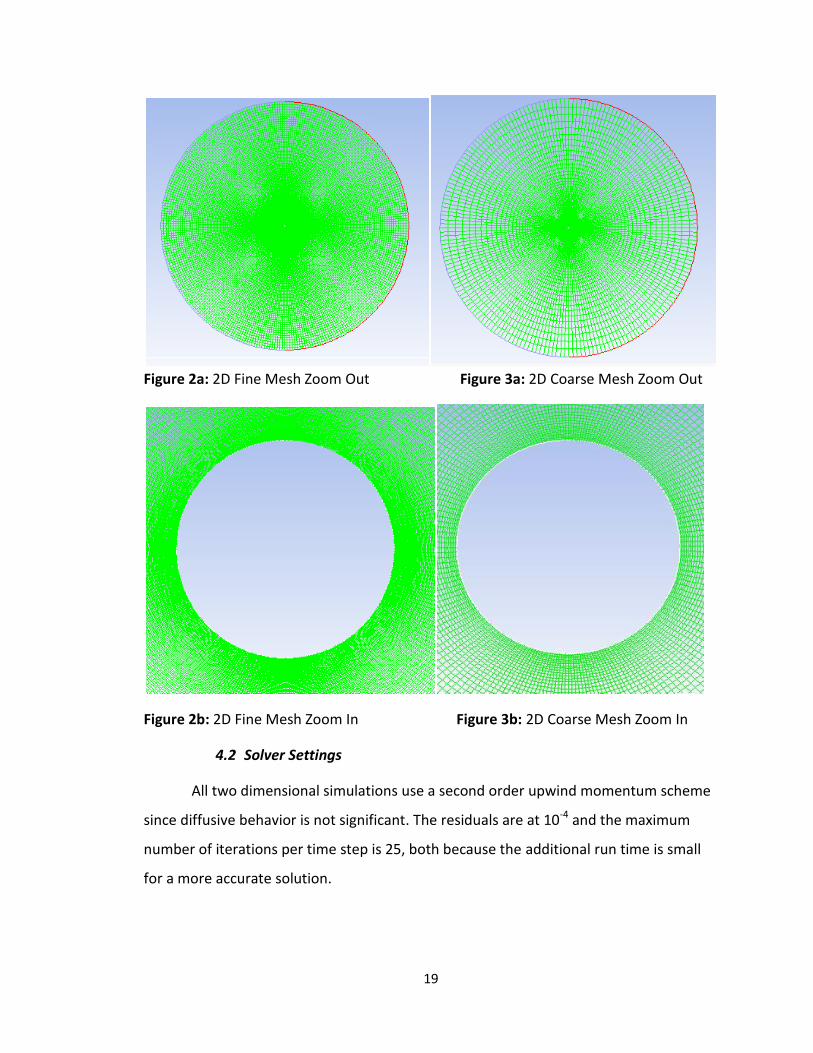
There are two meshes that are used in the two dimensional simulations, a coarse

mesh and a fine mesh as seen in Figs. 2 and 3. Table 1 gives statistics of the meshes. All

of the two dimensional results come from the fine mesh until section 4.5.

Table 1: Two Dimensional Mesh Statistics

Number of Cells Maximum volume (m3) Minimum Volume (m3)

Coarse Mesh 18,432 3.17E-03 4.31E-08

Fine Mesh 90,000 7.00E-04 7.09E-09

19

Figure 2a: 2D Fine Mesh Zoom Out Figure 3a: 2D Coarse Mesh Zoom Out

Figure 2b: 2D Fine Mesh Zoom In Figure 3b: 2D Coarse Mesh Zoom In

4.2 Solver Settings

All two dimensional simulations use a second order upwind momentum scheme

since diffusive behavior is not significant. The residuals are at 10-4 and the maximum

number of iterations per time step is 25, both because the additional run time is small

for a more accurate solution.

20

4.3 Results without Plasma Actuation

For all simulations the flow is in the positive x direction and the vortex induced

vibrations will be in the y direction.

Figure 4: Baseline Lift Coefficient for Fine Mesh

The lift coefficient demonstrates the magnitude and frequency of vortex induced

vibrations as well as flow development. As seen in Fig. 4 the cylinder experiences the

first major pressure difference around t=.05s. Around t=.225s shedding is fully

developed in both frequency and amplitude. This fully developed regime will be used to

dictate when the momentum source can be activated.

The following snapshot sequences demonstrate the development of the von

Kármán and Kelvin-Helmholtz vortices. Contour sequences of velocity magnitude,

vorticity magnitude and pressure coefficient are observed to analyze the transient flow

characteristics.

0 0.05 0.1 0.15 0.2 0.25 0.3 0.35 0.4 0.45 0.5-0.05

-0.04

-0.03

-0.02

-0.01

0

0.01

0.02

0.03

0.04

Flow Time (s)

Lift

Coeff

icie

nt

21

t=.01s t=.025s t=.05s

t=.075s t=.1s t=.125s

t=.15s t=.175s t=.2s

t=.225s t=.25s t=.275s

Figure 5: Velocity Magnitude Contours of Baseline Case with Fine Mesh [m/s]

22

Velocity magnitude contours from Fig. 5 with upper limit 5.5 m/s and lower limit

0 m/s demonstrate the transient velocity profile. Upon startup of the simulation at

t=.025s, two symmetric vortices are formed in the wake. At t=.05s the first major

pressure difference between the top half and the bottom half of the cylinder occurs;

indicated by the larger region of low velocity in the bottom half of the wake. At t=.1s

there are no longer two symmetric vortices and the cylinder begins to shed alternatively

from the top and bottom half of the cylinder. Until t=.25s the shedding regime is

developing until the full amplitude of shedding is reached as previously discussed.

Another interesting phenomenon is the nature of the transition from a

symmetric vortex wake to an asymmetric vortex wake. From t=.025s to t=.075s on the

location from the frontal stagnation point there is a region which feeds the

symmetric vortices in the wake. Note that during this time the wake is larger than the

fully developed regime and the separation point has moved upstream. At the instant

t=.1s an instability occurs, and the feeding region begins to alternate from the top and

bottom while the wake has asymmetric unsteady vortices for the rest of the simulation.

23

t=.01s t=.05s t=.1s

t=.15s t=.2s t=.25s

Figure 6: Vorticity Magnitude Contours of Baseline Case with Fine Mesh [s-1]

Vorticity contours from Fig. 6 with upper limit 3000s-1 and lower limit 0s-1

validate the velocity contours as well as reveal new information about the flow nature.

At t=.05s the first significant pressure difference appears between the top and bottom

halves of the cylinder, validated by the asymmetrical vortices from Fig. 5. Between

t=.05s and t=.1s the feeding regions disappear and at t=.1s the cylinder has transitioned

to asymmetric vortices.

A new phenomena is revealed in the snapshots at t=.15s through t=.25s, a sliding

vortex occurs on the downstream half of the cylinder. When a main vortex is completely

formed, the sliding vortex will be on the same side as seen at t=.25s. After the top

vortex is shed at t=.25s, the new forming vortex at the bottom half of the cylinder will

cause the sliding vortex to move along the cylinder wall and form near the bottom half,

opposite of t=.25s. This phenomenon repeats throughout the simulation and is due to

instability within the flow.

24

t=.01s t=.025s t=.05s

t=.075s t=.1s t=.125s

t=.15s t=.175s t=.2s

Figure 7: Pressure Coefficient Contours of Baseline Case with Fine Mesh

Pressure coefficient contours in Fig. 7 with upper limit 1 and lower limit -2.5 help

show how the induced vibrations develop. During the beginning of the simulation from

t=.01s to t=.025s the pressure coefficient is symmetric between the top and bottom half

of the cylinder on both the upstream and downstream side of the cylinder. This leads to

minimal induced vibrations as seen from Fig. 4. From t= .05s to t=.1s the cylinder is

shedding as seen by the wake asymmetry, but the flow is still developing. When the

flow is fully developed the shed vortices are indicated by the low pressure regions. On

25

the upstream side of the cylinder, the high pressure region is changing angle as vortices

are shed; this characteristic is always seen while shedding and is a source of vibrations

along with asymmetry in the wake.

4.4 Results with Plasma Actuation

Two dimensional simulations were used to characterize the impact of source

strength and grid size to a response before completing the three dimensional simulation

due to the computational cost. For the following two dimensional simulations, the flow

was allowed to fully develop until .24 seconds when the momentum source was

activated. Three different source strengths were explored to see the influence of the

momentum source strength on vortex shedding, some statistics are in Table 2.

Table 2: Statistics of Two Dimensional Momentum Source

Source Strength (Nm-3) Maximum Velocity (m/s) Force in Smallest Cell (mN)

Baseline Case 5.23 0

100,000 10.47 0.709

250,000 17.48 1.77

500,000 24.83 3.55

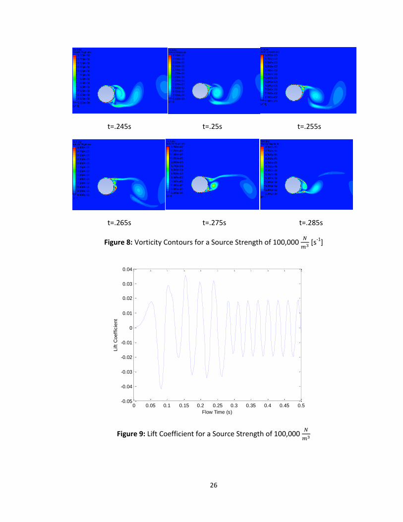
To assess the impact of a momentum source to the flow, only contours after the

source is activated will be shown. For the baseline flow regime the reader should review

section 4.3. For a momentum source with strength 100,000

, instantaneous snapshots

of vorticity magnitude are shown below.

26

t=.245s t=.25s t=.255s

t=.265s t=.275s t=.285s


[s-1]


0 0.05 0.1 0.15 0.2 0.25 0.3 0.35 0.4 0.45 0.5-0.05

-0.04

-0.03

-0.02

-0.01

0

0.01

0.02

0.03

0.04

Flow Time (s)

Lift

Coeff

icie

nt

27

Upon activation of the source, the separation location instantly changes as seen

at t=.245s in Fig. 8; also the previously existing vortices are no longer attached to the

cylinder. Between the times t=.255s and t=.265s there are trapped vortices in the wake,

helping the flow stabilize to the instances at t=.275s and t=.285s where shedding still

occurs. The new shedding regime has lower amplitude vibrations, but a slightly higher

frequency while still behaving in a periodic fashion as seen in Fig. 9. The momentum

source acts as a wall jet, changing the wake structure and behavior from the Coanda

effect. Pressure coefficient is not shown here as the difference between the baseline

case and the 100,000

case is small, although still an improvement. Velocity

magnitude will not be shown for any plasma case; only the maximum velocity occurring

in the wall jet will be recorded as in Table 2. The best insight on the flow structure can

be obtained from the vorticity magnitude contours.

A source strength of 250,000

was also tested, the vorticity and pressure

coefficient contours are shown below.

t=.245s t=.25s t=.255s

28

t=.265s t=.275s t=.285s


[s-1]


The momentum source again removes any attached vortices as seen at t=.245s

and the separation point is moved even further downstream. As seen from t=.265s

through t=.285s, the separation point is so far downstream that trapped vortices occur

in the flow from wall jet impingement. Fig. 11 shows shedding occurs at a higher

frequency and smaller overall amplitude than the baseline and the 100,000

case.

Shedding is no longer bounded by the constant amplitudes although still occurring in a

0 0.05 0.1 0.15 0.2 0.25 0.3 0.35 0.4 0.45 0.5-0.05

-0.04

-0.03

-0.02

-0.01

0

0.01

0.02

0.03

0.04

Flow Time (s)

Lift

Coeff

icie

nt

29

consistent frequency. Although resonance is generally based on frequency, the varying

amplitude may have an effect on resonance.

t=.245 t=.25s t=.255s

t=.265 t=.275s t=.285s

Figure 12: Pressure Coefficient Contours for a Source Strength of 250,000

The pressure contours in Fig. 12 show the impact of the momentum source on

the pressure that impacts shedding induced vibrations. Other than the roughly

region there are no locations where a low pressure coefficient occurs like the baseline

case. There are not significant vortices shed, and oscillating high pressure regions occur

in the wake as opposed to the baseline where the wake is comprised of alternating low

pressure regions from shedding. Looking at the frontal stagnation point, there is

miniscule change of the contour angle relative to the incoming flow direction, reducing

the induced vibrations dramatically as indicated by Fig. 11.

30

The next simulated momentum source had a strength of 500,000

, the

vorticity contours are shown below.

t=.245s t=.25s t=.255s

t=.265s t=.275s t=.285s


[s-1]


0 0.05 0.1 0.15 0.2 0.25 0.3 0.35 0.4 0.45 0.5-0.05

-0.04

-0.03

-0.02

-0.01

0

0.01

0.02

0.03

0.04

Flow Time (s)

Lift

Coeff

icie

nt

31

This momentum source strength eliminates shedding together. From the

initiation of the source at t=.245s, the strength of the source dominates the flow and

wall jet impingement completely changes the flow characteristics from the baseline

case. Trapped vortices occur in the wake and unsteadiness is associated with the flow as

seen in Fig. 14. As other previous cases, the amplitude of vibrations decrease while the

frequency of the vibrations increase. This source demonstrates periodic behavior in the

vibrations like the first source, indicating that there are certain strengths that will

produce periodic behavior and others that will not. This is likely based on a combination

of the source strength, flow regime and the mesh.

4.5 Mesh Dependency Results

To test the influence of a mesh on a given momentum source strength and

domain, a coarse mesh was used to compare results. The coarse mesh has the baseline

lift coefficient as seen in Fig. 15. Comparing the baseline fine mesh to the baseline

coarse mesh, the coarse mesh takes a longer time to develop into the full shedding

regime. This is due to a less refined mesh resulting in larger cell Reynolds numbers and

more dissipative behavior. However once developed around t=.275s, the frequency and

amplitude of shedding is comparable to the fine mesh results with only a very small

phase change occurring.

32

Figure 15: Baseline Lift Coefficients for Fine Mesh and Coarse Mesh

A source of strength 500,000

was used on the coarse mesh to see the impact

of identical source strength on a different mesh. The force in the smallest cell

corresponds to 21.55mN, nearly an order of magnitude higher than the fine mesh with

the same source strength. All sources on coarse mesh are activated after t=.3s to give

the flow ample time to develop.

t=.302s t=.305s t=.31s

0 0.05 0.1 0.15 0.2 0.25 0.3 0.35 0.4 0.45 0.5-0.05

-0.04

-0.03

-0.02

-0.01

0

0.01

0.02

0.03

0.04

Flow Time (s)

Lift

Coeff

icie

nt

Coarse Mesh

Fine Mesh

33

t=.315s t=.32s t=.325s


[s-1]


As seen in Fig. 17 this source completely dominates the wake structure and

behavior; eliminating shedding altogether. Upon activation of the source at t=.301s the

source reverses the direction of the vibration. As seen from t=.31s through t=.325s the

wall jet impingement from the Coanda effect removes any chance of vortices forming

and even forms a jet in the wake. The lift coefficient begins to asymptote to zero,

indicating that shedding has been eliminated and no longer has the ability to form.

The next simulation had the goal of matching the response of a 500,000

strength on fine mesh to an identical response on coarse mesh while using the same

0 0.05 0.1 0.15 0.2 0.25 0.3 0.35 0.4 0.45 0.5-0.04

-0.03

-0.02

-0.01

0

0.01

0.02

0.03

0.04

Flow Time (s)

Lift

Coeff

icie

nt

34

source domain. In attempt to do this the force in the smallest cells of each mesh were

set equal to each other. From Table 2, the force in the smallest cell for the 500,000

source strength in the fine mesh was 3.55mN. To match this force a strength of 82,250

was used for the coarse mesh. Again the source was activated at t=.301s.

t=.305s t=.315s t=.325s

t=.335s t=.345s t=.355s


[s-1]

35


The response is not the same between the coarse and fine mesh for a force of

3.55mN in the smallest cell as seen by comparing Fig. 14 and Fig. 19. This is due to the

fact that both meshes have the same source domain and the fine mesh has more cells

within that domain. When the applied force is integrated over both the coarse and fine

mesh, the fine mesh will experience a higher overall integrated force since the flow has

more cells to pick up force within the same source domain. This leads to a greater

response in a fine mesh for a given force in the smallest cell and source domain.

4.6 One Sided Source

The final two dimensional simulation was the influence of a momentum source

when applied to only one side of the cylinder. In this simulation the fine mesh was used

with a source strength of 500,000

(same strength as used in Fig. 14) applied only to

the top of the cylinder after t=.24s.

0 0.05 0.1 0.15 0.2 0.25 0.3 0.35 0.4 0.45 0.5-0.04

-0.03

-0.02

-0.01

0

0.01

0.02

0.03

0.04

Flow Time (s)

Lift

Coeff

icie

nt

36

t=.245s t=.25s t=.255s

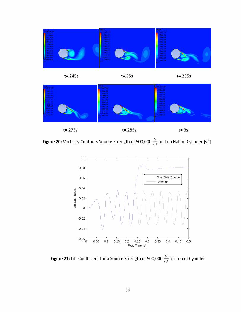
t=.275s t=.285s t=.3s

Figure 20: Vorticity Contours Source Strength of 500,000

on Top Half of Cylinder [s-1]


on Top of Cylinder

0 0.05 0.1 0.15 0.2 0.25 0.3 0.35 0.4 0.45 0.5-0.06

-0.04

-0.02

0

0.02

0.04

0.06

0.08

0.1

Flow Time (s)

Lift

Coeff

icie

nt

One Side Source

Baseline

37

Upon activation of the source, shedding still occurs until around t=.275s where a

vortex becomes trapped from the wall jet. As expected, the lift coefficient asymptotes

to zero after the trapped vortex occurs.

5. Three Dimensional Results

5.1 Mesh

Only one mesh is used for three dimensional simulations. The mesh is a one inch

diameter cylinder that is extruded two inches in the z direction. The cylinder was chosen

to be a two dimensional cylinder in a three dimensional domain to reduce the

computational cost associated with a larger domain that could capture flow features at

the ends of the cylinder. This paper only looks at the three dimensional wake impact of

the actuators, so ignoring the ends of the cylinders is a reasonable approximation. There

are three regions of body sizing within the mesh, one cylindrical and two boxes. The

cylindrical sizing is concentric with the cylinder and experiences the finest meshing to

allow proper refinement in the boundary layer region. The box closest to the cylinder is

to capture the forming vortices, and the box furthest from the cylinder is to capture

wake phenomenon. Inflation was used around the cylinder to help better capture the

boundary layer. The mesh has 16,898,711 elements and 3,183,491 nodes.

22)a 22)b

38

22)c

22)d

Figure 22: Three dimensional mesh a) Isometric view, b) Zoom out in Z-Direction,

c)Zoom In Z-direction d) Inflation on Cylinder Wall

39

5.2 Solver Settings

For the three dimensional simulations, a third order MUSCL momentum scheme

is used to combat the greater diffusive nature of the flow due to the formation of

streamwise vortices. The residuals are at 10-3 and the maximum number of iterations

per time step is 20, both because the run time cost is large if the settings were the same

as the two dimensional case. Aside from the velocity inlet and pressure outlet that have

the same settings as the two dimensional case, the other four walls of the box are

treated will a zero shear (symmetry) boundary condition.

5.3 Results without Plasma Actuation

The baseline case was simulated continuously for two weeks on the

Aerospace/Mechanical Engineering Linux Cluster using eight processors and memory

resources of 128GB. The flow is not fully developed due to insufficient computational

time as indicated by the vortices shedding far away from the cylinder in Fig. 23. These

results can still be used for the three dimensional simulation to see the general effects

on the wake for staggered actuators. Only single snapshots of velocity and vorticity at

t=1.926s will be shown as well as the transient lift coefficient for the baseline case. Data

was not taken upon starting the simulation, only after t=1.25s when shedding was at a

relatively steady frequency.

23a) 23b)

Figure 23: Three Dimensional Baseline Results a) Velocity [m/s] b) Vorticity [1/s]

40

Figure 24: Three Dimensional Baseline Lift Coefficient

The frequency of shedding is lower than the two dimensional fine mesh as seen

in Fig. 4, but the amplitude is significantly different. The lower frequency is due to the

dissipative nature of the solution due to the mesh not having proper refinement. The

amplitude difference is due to shedding occurring far away from the cylinder so the

pressure differences between the top and bottom half in the wake near the cylinder are

small.

5.4 Results with Varying Strength of Plasma Actuation

As learned from two dimensional simulations, the mesh and source strength

have a profound effect on the wake response. This led to the necessity that the three

dimensional mesh would also need to be tested for a reasonable response. Below are

three of the tested source strength velocity contours with the source across the entire

span of the cylinder, resulting in a two dimensional wake effect. Table 3 and Figs. 25, 26

display all of the source strengths tested on the three dimensional mesh. The goal with

these tests was to obtain a somewhat realistic but realizable impact on the wake and

separation point so when the source is applied three dimensionally there will be enough

resolution to see the flow structure.

-2.50E-05

-2.00E-05

-1.50E-05

-1.00E-05

-5.00E-06

0.00E+00

5.00E-06

1.00E-05

1.50E-05

1.25E+00 1.50E+00 1.75E+00 2.00E+00

Lift

Co

eff

icie

nt

Flow Time (seconds)

41

25a) 25b) 25c)

Figure 25: 3D Mesh Testing Velocity Magnitude Contours [m/s] a) Source

Strength=50,000

, b) Source Strength=175,000

, c) Source Strength=500,000

Figure 26: Curve of 3D Mesh Source Strengths vs Maximum Velocity [m/s]

Table 3: Statistics of 3D Source Strength Testing Source Strength [Nm-3 ] Max Velocity [m/s]

50000 6.79

100000 10.5

150000 13.4

175000 14.8

200000 16.1

500000 28.1

The results of these tests are similar to those of the two dimensional mesh; the

separation location is moved downstream and the wake size is reduced. Looking at Fig.

25c, if the strength is high enough trapped vortices will occur and nearly eliminate the

wake.

y = 0.0086x0.6166

0

5

10

15

20

25

30

0 200000 400000 600000

Max

imu

m V

elo

city

[m

/s]

Source Strength [Nm-3]

Series1

.5

42

5.5 Transient Results of a given Plasma Actuation Strength

Figure 27: Lift Coefficient for 3D Case with Source Strength 175,000

The three dimensional flow conditions were uploaded from the baseline

simulation in Fig. 23 at t=.38s, and ran in parallel with the baseline case due to

uncertainty that a periodic flow regime would occur. The computational resources were

the same for the baseline and source three dimensional simulations. From t=.38s until

t=.6s the flow in Fig. 27 ran without any momentum source. After t=.6s a source

strength of 175,000

was activated on the left half of the cylinder. One inch of the

cylinder had the source and the other side did not. The flow was allowed to develop

with the momentum source until a periodic behavior is reached. However, this did not

occur as seen from Fig. 27, as there is still unsteadiness and non-periodic behavior

associated with the flowfield. Snapshots were taken from t=1.111s to t=1.211s at

various locations in the flow to observe the flow physics with vorticity contours. A

source strength of 175,000

was used due to a reasonable change in flow separation

point allowing acceptable resolution of flow physics while still maintaining resemblance

43

to reality. The flow is in the positive x direction, and the spanwise direction is z. When

looking at the snapshots keep in mind the left half is activated and the right half is not.

90 degree location normal to x- Maximum Limit of 10,000s-1

t=1.111s t=1.113s

t=1.115s t=1.117s

t=1.119s t=1.211s

Figure 28: 90o Location on Cylinder Normal to X

44

As seen from Fig. 28 there is not any significant transient phenomena occurring.

What can be seen from these snapshots is that on the right hand side where there is no

momentum source, the flow has already separated from the cylinder. On the left half

where the source is located the flow is still attached, indicated by the low vorticity

magnitude on the cylinder wall. An interesting feature of all the snapshots is that for the

no source side, looking from right to left on the top and bottom of the cylinder wall the

vorticity magnitude increases near the wall. This is indicative of the effect the

streamwise vortex produces, which increases mixing of the wakes of the no source side

and the source side.

Edge of cylinder normal to x- Maximum Limit of 22,000s-1

t=1.111s t=1.113s

t=1.115s t=1.117s

45

t=1.119s t=1.211s

Figure 29: Edge of the Cylinder Normal to X

In these snapshots and subsequent snapshots there will be regions that appear

empty, do not be alarmed as they are just regions that exceed the maximum vorticity

contour limits. They were chosen to exist in certain snapshots to achieve better vorticity

resolution in other locations.

At the cylinder edge in the x-direction, the streamwise vortex can be clearly

seen. Notice how the location of the vortex center is not at one inch, but more around

an inch and a quarter in the z direction and within the source half; which was seen

experimentally by Bhattacharya[18]. Mixing of the wakes occur and the wakes on the

source side and on the bare side shrink due to the streamwise vortices. Between the top

and bottom streamwise vortices there is a transient region of vorticity, likely due to

shedding. Transient vortical structures also develop at the edge of the source side likely

from a combination of jet impingement and natural shedding.

46

Quarter inch past cylinder normal to x- Maximum Limit of 12,000s-1

t=1.111s t=1.113s

t=1.115s t=1.117s

t=1.119s t=1.211s

Figure 30: A Quarter of an Inch Past the Cylinder Normal to X

The snapshots in Fig. 30 show the wake outline the streamwise vortex induces.

On the left half, the source side appears to be shedding. On the edge of the source side

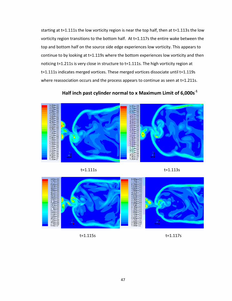
47

starting at t=1.111s the low vorticity region is near the top half, then at t=1.113s the low

vorticity region transitions to the bottom half. At t=1.117s the entire wake between the

top and bottom half on the source side edge experiences low vorticity. This appears to

continue to by looking at t=1.119s where the bottom experiences low vorticity and then

noticing t=1.211s is very close in structure to t=1.111s. The high vorticity region at

t=1.111s indicates merged vortices. These merged vortices dissociate until t=1.119s

where reassociation occurs and the process appears to continue as seen at t=1.211s.

Half inch past cylinder normal to x Maximum Limit of 6,000s-1

t=1.111s t=1.113s

t=1.115s t=1.117s

48

t=1.119s t=1.211s

Figure 31: A Half of an Inch Past the Cylinder Normal to X

From Fig. 31, streamwise vortices exhibit transient behaving merging and

dissociating behavior. An occurrence of merged vortices occur at t=1.111s, then

dissociation until recombination at t=1.119s. On the far source side there are alternating

regions of high vorticity, likely products of shedding. Another interesting feature of the

flow is the mixing of the far side source wake with the merged streamwise vortices. At

t=1.111s the beginning of a mixing phase occurs, and by t=1.115s a vortex is transferred.

By t=1.119s the transfer appears to have finished and the process begins again at

t=1.211s

Inch past cylinder normal to x- Maximum Limit of 2,500s-1

t=1.111s t=1.113s

49

t=1.115s t=1.117s

t=1.119s t=1.211s

Figure 32: An Inch Past the Cylinder Normal to X

Looking at Fig. 32 some phenomena that have been discussed before reoccur.

The far edge on the source side has the usual shedding and propagation downstream

occur as well as mixing with the streamwise vortices. The streamwise vortices also

dissociate and recombine as in Fig. 31. A new realization is the shedding on the top and

bottom of the bare side. Roughly every other frame from the top and bottom alternate

as the region of high vorticity, indicating vortex shedding.

50

Inch and a quarter in the z direction- Maximum Limit of 10,000s-1

t=1.111s t=1.113s

t=1.115s t=1.117s

t=1.119s t=1.211s

Figure 33: An Inch and a Quarter in the Z-Direction Normal to Z

The snapshots from Fig. 33 are located roughly where the centers of the

streamwise vortices are located. This region experiences separation points from both

the source and the bare side. For the source side separation point, the neutral situation

occurs at t=1.115s then a vortex is shed from the top location at t=1.117s and from the

bottom location at t=1.211s. From the bare side, shedding is hard to discern the exact

51

timescales due to the dissipative nature of the flow but vortices are clearly shedding

from the bare side. Note the separation point from the bare side has been moved

downstream but the vorticity contour has much more curvature off the separation point

when compared to the baseline regime in Fig. 23b. This additional curvature is due to

mixing from the streamwise vortices.

Edge of cylinder normal to x and inch and a quarter z direction- Maximum

Limit of 15,000s-1

t=1.111s t=1.113

t=1.115s t=1.117s

52

t=1.119s t=1.211s

Figure 34: Combined Views of Fig. 29 and Fig.33

The above snapshots are the combined snapshots of 1.25 inches in the z direction

and at the edge of the cylinder in the x direction rotated by roughly 45o in the z-x plane.

All of the images show that the top and bottom of the streamwise vortices closely

follow the separation location of the bare side. Shedding from the bare side is much

more evident in these snapshots.

t=1.111s t=1.113s

t=1.115s t=1.117s

53

t=1.119s t=1.121s

Figure 35: Instantaneous Isosurfaces of Vorticity Colored by X-Velocity

The isosurfaces shown in Fig. 35 further demonstrate much of the flow physics

previously discussed. The bare side and the source side have different separation points

and the streamwise vortex mixes the wakes of the bare and source side. The edges of

the cylinder behave as expected.

6. Conclusion

Vortex shedding is a phenomenon that should be accounted for when cylindrical

structures experience a crossflow. Plasma actuators have proven effective [1]-[4] in either

reducing or eliminating shedding. Previous models of various levels of complexity and

scope have been developed to demonstrate the effect of plasma actuators. Although

this paper does not go into the true physics and design parameters of the actuators,

using a momentum source with a reasonable domain and strength can give realistic

results when coupled into a computational fluid dynamics solver. From both the two

and three dimensional results the impact of source strength on the flow structure was

shown. For a given source domain and strength, the flow response is dictated by the

mesh sizing since the overall response depends on the integrated force in the source

domain, which is a function of cell size. In terms of flow response to source strength,

caution should be taken to avoid exciting a different resonant frequency while

eliminating the resonant frequency around the natural shedding frequency. Although

the three dimensional simulations did not fully develop in both the baseline case and

54

with the source, the results still generate general effects on the wake for staggered

actuators. The staggered actuators generated mixing from streamwise vortices, which

did not form at the contact point of the bare and source region but rather roughly a

quarter inch into the source region. This streamwise vortex induces mixing throughout

the wake until viscous damping removes the vortical structures.

7. Future Work

Since this paper focused only on modeling steady actuation, much investigation can

be completed in asymmetric or duty cycle forcing. Experimental work has been

completed by Jukes and Choi [2] and found a no shedding and lock on regime based on

frequency of actuation. Two dimensional simulations can be used to compare to

experimental work then the model can be extended to a three dimensional domain.

If similar computational resources and number of elements in the mesh is similar for

a three dimensional simulation, it is advised to start the baseline simulation as soon as

possible to allow the flow to fully develop.

55

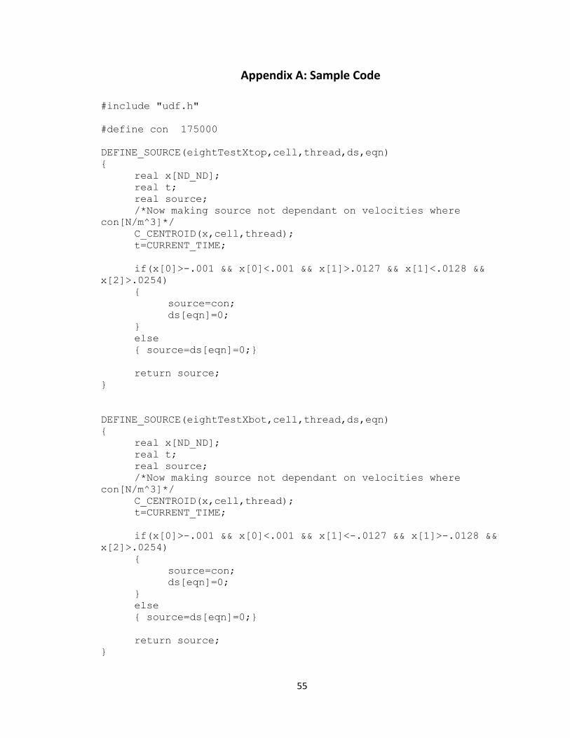
Appendix A: Sample Code

#include "udf.h"

#define con 175000

DEFINE_SOURCE(eightTestXtop,cell,thread,ds,eqn)

{

real x[ND_ND];

real t;

real source;

/*Now making source not dependant on velocities where

con[N/m^3]*/

C_CENTROID(x,cell,thread);

t=CURRENT_TIME;

if(x[0]>-.001 && x[0]<.001 && x[1]>.0127 && x[1]<.0128 &&

x[2]>.0254)

{

source=con;

ds[eqn]=0;

}

else

{ source=ds[eqn]=0;}

return source;

}

DEFINE_SOURCE(eightTestXbot,cell,thread,ds,eqn)

{

real x[ND_ND];

real t;

real source;

/*Now making source not dependant on velocities where

con[N/m^3]*/

C_CENTROID(x,cell,thread);

t=CURRENT_TIME;

if(x[0]>-.001 && x[0]<.001 && x[1]<-.0127 && x[1]>-.0128 &&

x[2]>.0254)

{

source=con;

ds[eqn]=0;

}

else

{ source=ds[eqn]=0;}

return source;

}

56

References

1. Thomas, Flint O., Thomas C. Corke, and Alexey Kozlov. “Plasma Actuators for

Cylinder Flow Control and Noise Reduction.” AIAA 46.8 (2008). 1921-1931.

2. Jukes, Timothy N., and Kwing-So Choi. “Flow control around a circular

cylinder using pulsed dielectric barrier discharge surface plasma.” Physics of

Fluids 21, 084103 (2009): 1-12.

3. Post, M.L., “Phased Plasma Actuators of Unsteady Flow Control.” MA Thesis,

University of Notre Dame, Notre Dame, IN, 2001.

4. Corke, Thomas C., C. Lon Enloe, and Stephen P. Wilkinson. “Dielectric Barrier

Discharge Plasma Actuators for Flow Control.” Annual Review of Fluid

Mechanics 42 (2009): 505-529. .

5. Haung, J. “Documentation of flow control separation on a linear cascade of

Pak-B blades using plasma actuators.” PhD thesis. University of Notre Dame.

Notre Dame, IN, 2005.

6. Nikita Bibinov, Priyadarshini Rajasekaran, Philipp Mertmann Dirk Wandke,

Wolfgang Viöl and Peter Awakowicz (2011). “Basics and Biomedical

Applications of Dielectric Barrier Discharge (DBD)”, Biomedical Engineering,

Trends in Materials Science, Mr Anthony Laskovski (Ed.), ISBN: 978-953-307-

513-6, InTech, DOI: 10.5772/13192. Available from:

http://www.intechopen.com/books/biomedical-engineering-trends-in-

materials-science/basics-and-biomedical-applications-of-dielectric-barrier-

discharge-dbd-

57

7. Incropera, Frank P., David P. Dewitt, Theodore L. Bergman, and Adrienne S.

Lavine. “Principles of Heat and Mass Transfer.” Singapore: John Wiley &

Sons, 2013. Print.

8. Asyikin, Muhammad Tedy, “CFD Simulation of Vortex Induced Vibration of a

Cylindrical Structure” MA Thesis. Norwegian University of Science and

Technology, Trondheim, Norway, 2012.

9. Howatson, A.M. “An Introduction to Gas Discharges”. Oxford: Permagon

Press, 1976. Print.

10. Jayaraman, B, Cho,Y-C, Shyy, W. “Modeling of Dielectric Barrier Discharge

Plasma Actuator.” Physics of Fluids 21, 053304 (2009): 1-15.

11. Roth, JR, Sherman D, Wilkinson SP. “Electrohydrodynamic Flow Control With

Glow Discharge Surface Plasma.” AIAA 38 (2000):1166-1172.

12. Roth, JR, and Dai X. “Optimization of the aerodynamic plasma actuator as an

EHD electrical device.” Presented at AIAA Aerosp. Sci. Meet. Exhibit, 44th,

Reno, AIAA Pap. No. 2006-1203.

13. Enloe CL, McLaughlin TE, VanDyken RD, Kachner KD, Jumper EJ. “Mechanisms

and responses of a single-dielectric barrier plasma actuator: geometric

effects.” AIAA J. 42:595–604 (2004).

14. Gibalov V, Pietsch G. “The development of dielectric barrier discharges in gas

gaps and surfaces.” J. Phys. D 33:2618–36 (2000).

58

15. Kozlov KV, Wagner H-E, Brandenburg R, Michel P. “Spatio-temporally

resolved spectroscopic diagnostics of the barrier discharge in air at

atmospheric pressure.” J. Phys. D 34:3164–76 (2001).

16. Font GI, Morgan WL. “Plasma discharges in atmospheric pressure oxygen for

boundary layer separation control.” Presented at AIAA Fluid Dyn. Conf.

Exhibit, 35th, Toronto, AIAA Pap. No. 2005-4632 (2005).

17. Orlov D, Corke T. “Numerical simulation of aerodynamic plasma actuator

effects.” Presented at AIAA Aerosp. Sci. Meet. Exhibit, 43rd, Reno, AIAA

Paper 2005-1083 (2005).

18. Bhattacharya, Samik. “Investigation of Three Dimensional Forcing of Cylinder

Wake with Segmented Plasma Actuators and the Determination of the

Optimum Wavelength of Forcing.” PhD Dissertation, The Ohio State

University, Columbus, OH, 2013.

THE OHIO STATE UNIVERSITY- DEPARTMENT OF AEROSPACE/ MECHANICAL ENGINEERING€¦ · · 2014-04-11THE OHIO STATE UNIVERSITY- DEPARTMENT OF AEROSPACE/ MECHANICAL ENGINEERING ... An

Documents