The OCO-3 mission; measurement objectives and expected ...

The OCO-3 mission; measurement objectives and expectedperformance based on one year of simulated dataAnnmarie Eldering1, Tommy E. Taylor2, Chris W. O’Dell2, and Ryan Pavlick1

1Jet Propulsion Laboratory, California Institute of Technology, Pasadena, CA, 91109, USA.2Cooperative Institute for Research in the Atmosphere, Colorado State University, Fort Collins, CO, 80521, USA.

Correspondence: Annmarie Eldering ([email protected])

Abstract. The Orbiting Carbon Observatory-3 (OCO-3) is NASA’s next instrument dedicated to extending the record of the

dry-air mole fraction of column carbon dioxide (XCO2) and solar-induced fluorescence (SIF) measurements from space. The

current schedule calls for a launch in the first half of 2019 via a Space-X Falcon 9 and Dragon capsule, with installation as an

external payload on the Japanese Experimental Module Exposed Facility (JEM-EF) of the International Space Station (ISS).

The nominal mission lifetime is 3 years. The precessing orbit of the ISS will allow for viewing of the earth at all latitudes less5

than approximately 52◦, with a ground repeat cycle that is much more complicated than the polar orbiting satellites that so far

have carried all of the instruments capable of measuring carbon dioxide from space.

The grating spectrometer at the core of OCO-3 is a direct copy of the OCO-2 spectrometer, which was launched into a

polar orbit in July 2014. As such, OCO-3 is expected to have similar instrument sensitivity and performance characteristics to

OCO-2, which provides measurements of XCO2 with precision better than 1 ppm at 3 Hz with each viewing frame containing10

8 footprints of approximate size 1.6 by 2.2 km. However, the physical configuration of the instrument aboard the ISS, as well

as the use of a new pointing mirror assembly (PMA), will alter some of the characteristics of the OCO-3 data, compared to

OCO-2. Specifically, there will be significant differences from day to day in the sampling locations and time of day. In addition,

the flexible PMA system allows for a much more dynamic observation mode schedule.

This paper outlines the science objectives of the OCO-3 mission and, using a simulation of one year of global observations,15

characterizes the spatial sampling, time of day coverage, and anticipated data quality of the simulated L1b. After application of

cloud and aerosol prescreening, the L1b radiances are run through the operational L2 full physics retrieval algorithm, as well

as post-retrieval filtering and bias correction, to examine the expected coverage and quality of the retrieved XCO2 and to show

how the measurement objectives are met. In addition, results of the SIF from the IMAP-DOAS algorithm are analyzed. This

paper focuses only on the nominal nadir-land and glint-water observation modes, although on-orbit measurements will also be20

made in transition and target modes, similar to OCO-2, as well as the new “snapshot” area mapping mode.

1 Introduction

As called for in NASA’s Climate Architecture Report (June 2010), the Orbiting Carbon Observatory-3 (OCO-3) was built from

spare parts during the construction of OCO-2 to be made available as an instrument of opportunity. After assessment of various

1

Atmos. Meas. Tech. Discuss., https://doi.org/10.5194/amt-2018-357Manuscript under review for journal Atmos. Meas. Tech.Discussion started: 5 November 2018c© Author(s) 2018. CC BY 4.0 License.

options, the decision was made in 2013 to design and build the OCO-3 payload for operation on the International Space Station

(ISS). The primary scientific objective of OCO-3 is to provide global, dense, high-precision measurements of the dry-air mole

fraction of column carbon dioxide (XCO2) and solar-induced fluorescence (SIF) from space. A planned 3 year lifetime aboard

the ISS will allow for continuation of the international measurement record of CO2 that began in earnest with the Japanese

GOSAT satellite (January 2009 to present) (Kuze et al., 2009), followed by the NASA OCO-2 mission (July 2014 to present),5

and most recently by the Chinese TANSAT (December 2016 to present) (Yang et al., 2018). Furthermore, a 2019 launch of

OCO-3 would provide overlap for future planned missions such as GOSAT-2 (planned 2018 launch) (Nakajima et al., 2012),

the MicroCARB mission from CNES (planned 2021 launch) (Buil et al., 2011), and possibly even with the recently selected

NASA GeoCarb mission (O’Brien et al., 2016), which has a planned 2022 launch. Because of the relatively small variations

in atmospheric CO2 globally, it is critical to understand how the data products from various sensors intercompare at levels less10

than their precision, which is 0.1% for both OCO-2 and OCO-3. It is worth noting that all of the sensors mentioned above are

polar orbiting, with the exception of OCO-3 (precessing) and GeoCarb, which is the first planned geostationary observation

system for measuring XCO2.

The nominal planned viewing strategy of OCO-3 is to take down-looking nadir viewing measurements over land to minimize

the probability of cloud and aerosol contamination. Over water measurements will be taken near the specular reflection spot15

(glint viewing) to maximize the signal over the low reflectivity surface. However, unlike OCO-2, which performs complex

maneuvers of the entire satellite bus to observe ground targets, the OCO-3 instrument will be fitted with an agile 2-D pointing

mechanism, i.e., a pointing mirror assembly (PMA). This will allow for rapid transitions between nadir and glint mode (less

than 1 minute). The PMA will also allow for target mode observations, similar to those taken by OCO-2, typically at Total

Column Carbon Observation Network (TCCON) ground sites for use in validation (Wunch et al., 2010). The PMA will provide20

the ability to scan large contiguous areas (order 80 km by 80 km), such as cities and forests, on a single overpass. This will

be known as "snapshot" mode and will allow for fine scale spatial sampling of CO2 and SIF variations unlike what can be

done with any current satellite system. If OCO-2 and OCO-3 operate concurrently, the snapshot mode can be used to gather

a significant fraction of overlapping data. However, this paper deals exclusively with the two main viewing modes (nadir-land

and glint-water), while a detailed discussion of snapshot mode is deferred to a companion paper.25

The sampling that will be provided by OCO-3 aboard the precessing ISS will differ significantly compared to the polar

orbits of OCO-2 and GOSAT. The overpasses will not always occur at the same local time of day for a given point on the earth,

which has implications with respect to the diurnal cycle of both clouds and aerosols (which contaminate the observations of

XCO2) and studies of the carbon cycle, which itself has a strong diurnal variation. The precession in time-of-day sampling

will be especially informative for the SIF observations with respect to studying the biosphere response (both natural and30

anthropogenic) to changes in sunlight.

The international record of satellite remote sensing of CO2 has extended across a number of measurement platforms, e.g.

SCIAMACHY (2002-2012), Aqua-AIRS (2002-present) , GOSAT (2009-present), TANSAT (2016-present) and is being used

to quantify several aspects of the carbon cycle. The CO2 seasonal cycle has been studied with SCIAMACHY and GOSAT

data (e.g., (Buchwitz et al., 2015; Lindqvist et al., 2015; Reuter et al., 2013; Wunch et al., 2013)). The GOSAT measurements35

2


have been used to characterize a number of relatively large disturbances to the carbon cycle, including reduced carbon uptake

in 2010 due to the Eurasia heat wave (Guerlet et al., 2013), larger than average carbon fluxes in tropical Asia in 2010 due to

above-average temperatures (Basu et al., 2014), and anomalous carbon uptake in Australia (Detmers et al., 2015). In addition,

Parazoo et al. used GOSAT XCO2 and SIF estimates to better understand the carbon balance of southern Amazonia (Parazoo

et al., 2014), while Ross et al. used GOSAT data to obtain information on wildfire CH4:CO2 emission ratios (Ross et al., 2013).5

Relative to earlier carbon dioxide measurements from space, OCO-2 is providing a much denser data set (in both time and

space) with higher precision in retrieved XCO2. The publicly available B7 version of the OCO-2 data ((https://disc.gsfc.nasa.gov/))

has recently been used to quantify changes in tropical carbon fluxes (Liu et al., 2017) and the equatorial Pacific ocean (Chat-

terjee et al., 2017), due to the strong 2015 El Nino. Schwandner et al. (2017) highlighted localized sources detected by OCO-2,

while Eldering et al. (2017b) provided an extensive global view of the atmospheric carbon dioxide as observed from OCO-210

after its first two years in space.

In order to continue the international measurement record of global carbon dioxide from space, NASA plans to operate

OCO-3 from the ISS for a period of about 3 years, beginning nominally in early 2019. Since there are a number of new

considerations related to the unique viewing and sampling from this platform, it is desirable to study the expected performance

of the instrument prior to launch. To do this we generated one full year of simulated OCO-3 measurements, on which we15

ran the current versions of the OCO-2 prescreeners and L2 retrieval, as well as the post-processing quality filtering and bias

correction. The bulk of this paper is based on these simulations to evaluate expected data quality and data density from OCO-3

aboard the ISS.

The paper is organized as follows. Section 2 provides an overview of the OCO-3 mission, the science objectives and planned

measurement modes. In Section 3, the generation of one year of simulated L1b radiances using realistic geometry, instrument20

characteristics and meteorology is detailed. Section 4 discusses properties of the retrieved XCO2 from OCO-3 using effectively

operational algorithms for retrieval, filtering, and bias correction. Overall analysis of the results are presented in Section 5.

Particular focus is given to the temporal and spatial coverage, expected signal-to-noise ratios, and XCO2 and SIF errors.

Finally, Section 6 provides a summary of the expected performance of the OCO-3 mission based on these simulations.

2 The OCO-3 science objectives and measurement overview25

Like OCO-2, the OCO-3 mission has been designed to collect a dense set of precise measurements of XCO2 with a small

footprint. The scientific objective of the mission is to quantify variations of XCO2 with the precision, resolution, coverage,

and temporal stability needed to improve our understanding of surface sources and sinks of carbon dioxide on regional scales

('1000 km by 1000 km) and the processes controlling their variability over the seasonal cycle. The measurement objective

is to quantify the dry air column carbon dioxide ratio (the total column of carbon dioxide normalized by the column of dry30

air) to better than 1 ppm for collections of 100 footprints, the same objective as OCO-2. The footprint size is equal to or less

then 4 km2, and changes in aspect ratio with the viewing geometry. The OCO-3 mission will also provide a measurement of

solar-induced fluorescence (SIF), again with similar characteristics as OCO-2. As will be discussed in Section 3, the sampling

3


characteristic from the ISS will result in changing latitudinal coverage each month, such that the regions where sources and

sinks can be quantified will vary in time. The nominal measurement operation mode will be to collect data in nadir viewing

over land and glint viewing over oceans, with a variable number of target and snapshot mode measurements integrated each

day.

In addition, the OCO-3 mission also has the potential to contribute to carbon cycle science beyond its primary objective. The5

current plan includes the nearly simultaneous installation of three other instruments aboard the ISS that are focused on various

aspects of the terrestrial carbon cycle (Stavros et al., 2017). This includes NASA’s Global Ecosystem Dynamics Investigation

(GEDI), which is a lidar instrument designed to make observations of forest vertical structure to assess the above-ground carbon

balance of the land surface and investigate its role in mitigating atmospheric CO2 in the coming decades (Dubayah et al., 2014;

Stysley et al., 2015). NASA/JPL’s Ecosystem Spaceborne Thermal Radiometer Experiment on Space Station (ECOSTRESS)10

will measure evapotranspiration and assess plant stress and its relationship to water availability (Fisher et al., 2015; Hulley

et al., 2017) Finally, the Hyperspectral Imager Suite (HISUI) from JAXA will have a multi-band spectrometer with a focus

on identifying plant types (Matsunaga et al., 2015, 2017). The integration of these data, along with OCO-3 measurements of

XCO2 and SIF, have the potential to inform our understanding of many aspects of ecosystem processes (Stavros et al., 2017).

An additional enhancement to the OCO-3 data set will be provided by the currently operating OCO-2 instrument if its15

special pointing capability is synchronized with this suite of instruments to view specific ground targets. A second opportunity

for OCO-3 relates to the use of the snapshot mode to focus on emissions hotspots, such as emissions from cities and power

plants, or from natural sources such as volcanoes and wildfires. If OCO-2 and OCO-3 operate concurrently, complementary

sampling could maximize the insights on the sources and sinks of carbon dioxide.

2.1 The OCO-3 instrument payload20

At the core of OCO-3 is a three-band grating spectrometer built as a spare for the OCO-2 instrument, which measures reflected

sunlight (Crisp et al., 2017; Eldering et al., 2017a). The oxygen A-band (O2 A-band) measures absorption by molecular

oxygen near 0.76µm, while two carbon dioxide bands, labelled here as the weak and strong CO2 bands, are located near 1.6

and 2.0µm, respectively. The O2 A-band is sensitive to the atmospheric path length observed due to the absorption by oxygen,

and is used to estimate the apparent surface elevation and as part of the detection of clouds. This band also provides sensitivity25

to solar-induced fluorescence (SIF), a small amount of light emitted during plant photosynthesis (Frankenberg et al., 2012).

The weak CO2 and strong CO2 bands provide sensitivity to carbon dioxide, with peaks at different vertical heights, but are

also used as part of the cloud detection scheme since they are particularly sensitive to the wavelength dependence of aerosol

scattering and absorption. Estimates of XCO2 are derived from these spectra using an optimal estimation retrieval method that

integrates detailed models of the physics of the atmosphere (Bösch et al., 2006; Connor et al., 2008; O’Dell et al., 2012).30

The instrument has 1016 spectral elements in each band, with 160 pixels averaged in groups of 20 along the slit, creating eight

spatial footprints. The entrance optics have been modified to reduce the magnification from 2.4:1 to 1:1, to maintain similar

footprint sizes given the lower altitude of the ISS, which typically flies at '404 km, compared to OCO-2 at '705 km. This

magnification change will result in OCO-3 footprints that are < 4 km2, comparable to the 3 km2 of OCO-2. The instrument

4


field of view, i.e., the frame, will be approximately 13 km, or 1.6 km width per eight footprints, and the spacecraft motion

covers '2.2 km during the 0.33 seconds of integration time. The rate of data collection will be approximately 1 million sets of

3 spectral band measurements per day, before considering ISS limitations discussed in Section 2.3.

The OCO-3 project inherited a fully characterized spectrometer from the OCO-2 project, which was designed for integration

on a LeoStar spacecraft. For utilization on the ISS JEM-EF, a number of adaptations were required (Basilio et al., 2013). These5

include redesign of the thermal system, updates to the electrical system, and updates to the data flow from the instrument to

the data processing center at JPL. These changes do not fundamentally change the radiometric characteristics, and therefore

the science data quality, so will not be discussed in this paper. As described in the following section, a new pointing mirror

assembly was also required for OCO-3.

2.2 OCO-3 pointing mirror assembly overview10

A design change that impacts the radiometric characteristics of the data is the addition of a pointing mirror assembly (PMA).

The PMA is required to allow non-nadir observations from the fixed position on the ISS, unlike the currently operating OCO-2,

which maneuvers the entire spacecraft to point. Two important design requirements of the PMA were to allow quick movement

through a large range of angles, and that the movement not impart any angular dependent polarization or radiance changes in the

measurements. To meet these objectives a variation of the pointing system designed for the Glory Aerosol Polarimetry Sensor15

(APS) (Persh et al., 2010) was selected. This system relies on a single pair of matched mirrors in an orthogonal configuration

that impart less than 0.05% change to the polarization (Mishchenko et al., 2007). For the OCO-3 PMA the concept was extended

to a 2-axis pointing system. There are two elements; one controlling the azimuthal (cross-track) angle, and the other controlling

the elevation (along-track) angle. Although the PMA itself does not change the polarization of the light more them 0.1%, there

are polarization implications, since the image of the slit is rotated as a function of the change in the PMA, primarily driven20

by the elevation (along-track) angle. It is worth noting that reflected sunlight is naturally polarized by its interaction with the

earth’s surface and atmosphere, especially over water.

Early in the mission design, a trade study was performed, evaluating the expected signal with and without the installation of

an additional polarization scrambler, i.e., a polarization nulling optical component. Without a scrambler, the signal measured

by the instrument is large when the polarization of the incident light is aligned with the axis of polarization sensitivity of25

the instrument, i.e, polarization angle of zero. However, the measured signal decreases towards zero as the polarization of the

incoming light rotates orthogonal to the axis of instrument polarization (polarization angle of 90 degrees). Inserting a scrambler

would make the polarization orientation of the incoming light random, regardless of the position of the PMA, but would reduce

the signal by nearly 50% compared to having no scrambler. In addition, the analysis showed that a single optical element that

could scramble light at all of the OCO-3 wavelengths could not be manufactured and characterized to the required precision.30

Lastly, the volume and coverage of data with sufficient signal in the no-scrambler case was predicted to be more than sufficient

to meet the science objectives. Therefore, OCO-3 will be operated without a polarization scrambler.

As will be discussed in more detail in Section 5.1, the PMA is one element that contributes to a change in the overall light

throughput of OCO-3 compared to OCO-2. In the O2 A-band, each mirror has a reflectivity of 95.4%, so the 4 mirror PMA

5


system has an effective transmission of 83%. The weak and strong CO2 band overall transmissions are higher, at 93% and

95%, respectively.

The thermal vacuum testing of OCO-3 has been finalized and analysis of the data is underway, with completion planned in

the second half of 2018. Details of the measurement performance and how it compares to the instrument requirements will be

reported in a forthcoming manuscript.5

2.3 Sampling from the International Space Station - routine measurements

The ISS orbit is nearly circular about the earth, with altitudes that ranges from 330 km to 410 km. The planned altitude during

the time of OCO-3 operation is 405 km. With a ground-track velocity of 27,600 km/h (7.667 km/s), one orbit around the earth

is completed in about 92 minutes. The inclination of the orbit is 51.6◦, which limits the latitudinal range that can be sampled

by OCO-3. These orbital parameters result in a precessing orbit, meaning the local overpass time varies across all hours of the10

day over the course of a year.

OCO-3 will dynamically control the viewing mode along each orbit via the PMA, with routine data collection consisting of

nadir and glint measurements. Over land, where both nadir and glint measurements provide sufficient signal, the measurements

will primarily be made in nadir mode, where both the optical path length and statistical probability of observing clouds are

minimized.15

Glint measurements are necessary over the ocean, as the surface reflectivity is not large enough to produce adequate signal,

except in a few cases. A small offset from the true glint spot will be included to avoid saturation of the instrument. While the

glint measurements provide larger signal over oceans, the longer optical path lengths and enlarged footprint of this geometry

also make these measurements more sensitive to cloud cover (Miller et al., 2007).

The transition time for the PMA is required to be less than 50 seconds between nadir and glint modes, which translates20

into approximately 380 km along-track. In testing with the flight hardware, all moves were made within 10 seconds, which

corresponds to about 75 km along track. Mission planning assumes the required 50 s move time, and thus, similarly to GOSAT,

small land masses in the ocean will be measured in glint mode, while continental scale areas (areas that will be sampled for

more than 200 seconds) will be measured in nadir mode. Unfortunately, this means that most inland fresh water bodies will

be observed in nadir mode and will therefore not provide useful retrievals due to low signal to noise ratios. This will include25

bodies as large as, for example, the Great Lakes of North America. However, bodies of water as large as the Mediterranean Sea

will be sampled in glint viewing. This is one of the key differences from OCO-2, where the measurement mode is specified

orbit by orbit.

A subtlety of OCO-3 relative to OCO-2 is that, for nadir-land observations, the slit will remain perpendicular to the direction

of flight since the instrument is not rotated to maintain measurements in the principle plane. This will produce a constant swath30

width of about 13 km, as depicted in Figure 1, which provides a best-guess representation of several frames viewing the Los

Angeles metropolitan area. The ground footprint for glint mode measurements, however, will more closely resemble that of

OCO-2, as the PMA will rotate to view near the specular reflection point.

6


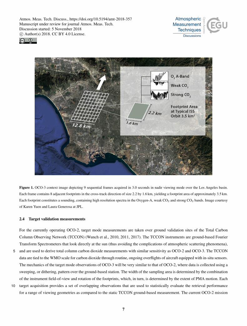
Figure 1. OCO-3 context image depicting 9 sequential frames acquired in 3.0 seconds in nadir viewing mode over the Los Angeles basin.

Each frame contains 8 adjacent footprints in the cross-track direction of size 2.2 by 1.6 km, yielding a footprint area of approximately 3.5 km.

Each footprint constitutes a sounding, containing high resolution spectra in the Oxygen-A, weak CO2 and strong CO2 bands. Image courtesy

of Karen Yuen and Laura Generosa at JPL.

2.4 Target validation measurements

For the currently operating OCO-2, target mode measurements are taken over ground validation sites of the Total Carbon

Column Observing Network (TCCON) (Wunch et al., 2010, 2011, 2017). The TCCON instruments are ground-based Fourier

Transform Spectrometers that look directly at the sun (thus avoiding the complications of atmospheric scattering phenomena),

and are used to derive total column carbon dioxide measurements with similar sensitivity as OCO-2 and OCO-3. The TCCON5

data are tied to the WMO scale for carbon dioxide through routine, ongoing overflights of aircraft equipped with in-situ sensors.

The mechanics of the target mode observations of OCO-3 will be very similar to that of OCO-2, where data is collected using a

sweeping, or dithering, pattern over the ground-based station. The width of the sampling area is determined by the combination

of the instrument field-of-view and rotation of the footprints, which, in turn, is determined by the extent of PMA motion. Each

target acquisition provides a set of overlapping observations that are used to statistically evaluate the retrieval performance10

for a range of viewing geometries as compared to the static TCCON ground-based measurement. The current OCO-2 mission

7


captures 1 or 2 target measurements per day, such that the total number gathered over the mission lifetime has been sufficient

to perform validation (Wunch et al., 2017). OCO-3 will follow this basic strategy, although for some sites, where there are very

few measurements in some seasons, e.g., at high latitudes in the winter, OCO-3 will potentially take more target measurements

per day if it will improve the seasonal coverage for these sites.

2.5 Snapshot mode measurements5

The agile pointing system of OCO-3 will also allow for collection of data in new spatial patterns relative to OCO-2. We have

designed a snapshot mode, which can simply be thought of as a target observation with two dimensional sweeping, i.e., from

side to side as well as back and forth. In this way, an area on the order of 80 km by 80 km can be sampled. The types of areas

that will be sampled include CO2 emission hotspots, terrestrial carbon focus areas, and volcanos. Based on analysis of fossil

fuel emissions and uncertainties of the emissions estimates (Oda and Maksyutov, 2011; Oda et al., 2018), a nominal sampling10

strategy for the emission hotspots is being developed. Preliminary results suggest that 50 to 100 snapshots per day will be

collected, consuming up to 200 of the approximately 650 day-light orbit minutes, i.e., 25 to 30% of the data volume. This will

provide a novel data set for exploration by the scientific community that is focused on the remote sensing of greenhouse gases

and SIF from space. The full details of the new snapshot mode will be presented in a future companion paper.

3 Simulated geometry, meteorology and L1b dataset15

In this section, we discuss the simulation of OCO-3 data in terms of viewing geometry, meteorology and observed radiometric

quantities such as data density and SNR, the latter of which is the primary driver of instrument precision. This will enable us to

realistically discern the effects that the ISS orbit will have on our data products, in comparison to the sun-synchronous afternoon

orbits of OCO-2. The generation of OCO-3 L1b radiances presented in this paper followed the same basic methodology as that

used in previously published work on both GOSAT and OCO-2, e.g., (Bösch et al., 2006; O’Brien et al., 2009; O’Dell et al.,20

2012).

3.1 Simulated OCO-3 observation geometry

Actual ISS ephemeris data for the year 2015 were used to provide position and velocity vectors of the space station each second

over the course of a year. To create a manageable data set for this work, samples were taken only once every 10 seconds, rather

than at the true 3 Hz collection rate of the OCO-3 instrument. Also, only one sounding per frame, rather than eight, was used25

since the truth models lack the fidelity necessary for such high spatial resolution. The analysis presented in this work focuses

on nadir and glint observation modes only, i.e., ignores transition, target and snapshot modes. This provides a baseline of the

densest possible nadir and glint data if all the other viewing modes were disabled. As was mentioned in Sect. 2.5, it is estimated

that as much as 25-30% of the data volume will be collected in snapshot mode, with some additional small amount (order of a

few percent) collected in target mode.30

8


Although the ISS latitude varies between ± 51.6◦, the OCO-3 PMA allows for measurements extending beyond this range

to approximately± 55.5◦ latitude. However, we found that useful measurements, i.e., those assigned a good XCO2 quality flag

as described in Sect. 4.3 and 5.3, are obtained at latitudes less than about 52◦, where the solar zenith angle is less than about

73◦. The exact range of latitudes measured on any given day will vary, depending on solar geometry and mechanical viewing

constraints from the ISS, as described below.5

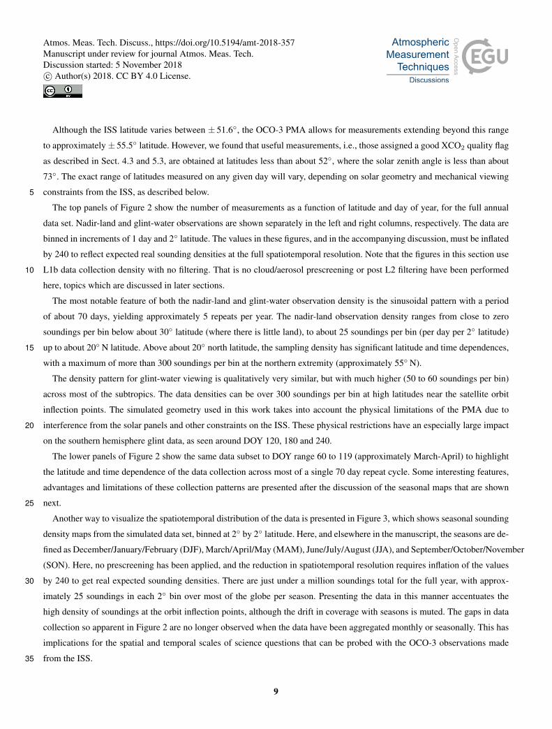
The top panels of Figure 2 show the number of measurements as a function of latitude and day of year, for the full annual

data set. Nadir-land and glint-water observations are shown separately in the left and right columns, respectively. The data are

binned in increments of 1 day and 2◦ latitude. The values in these figures, and in the accompanying discussion, must be inflated

by 240 to reflect expected real sounding densities at the full spatiotemporal resolution. Note that the figures in this section use

L1b data collection density with no filtering. That is no cloud/aerosol prescreening or post L2 filtering have been performed10

here, topics which are discussed in later sections.

The most notable feature of both the nadir-land and glint-water observation density is the sinusoidal pattern with a period

of about 70 days, yielding approximately 5 repeats per year. The nadir-land observation density ranges from close to zero

soundings per bin below about 30◦ latitude (where there is little land), to about 25 soundings per bin (per day per 2◦ latitude)

up to about 20◦ N latitude. Above about 20◦ north latitude, the sampling density has significant latitude and time dependences,15

with a maximum of more than 300 soundings per bin at the northern extremity (approximately 55◦ N).

The density pattern for glint-water viewing is qualitatively very similar, but with much higher (50 to 60 soundings per bin)

across most of the subtropics. The data densities can be over 300 soundings per bin at high latitudes near the satellite orbit

inflection points. The simulated geometry used in this work takes into account the physical limitations of the PMA due to

interference from the solar panels and other constraints on the ISS. These physical restrictions have an especially large impact20

on the southern hemisphere glint data, as seen around DOY 120, 180 and 240.

The lower panels of Figure 2 show the same data subset to DOY range 60 to 119 (approximately March-April) to highlight

the latitude and time dependence of the data collection across most of a single 70 day repeat cycle. Some interesting features,

advantages and limitations of these collection patterns are presented after the discussion of the seasonal maps that are shown

next.25

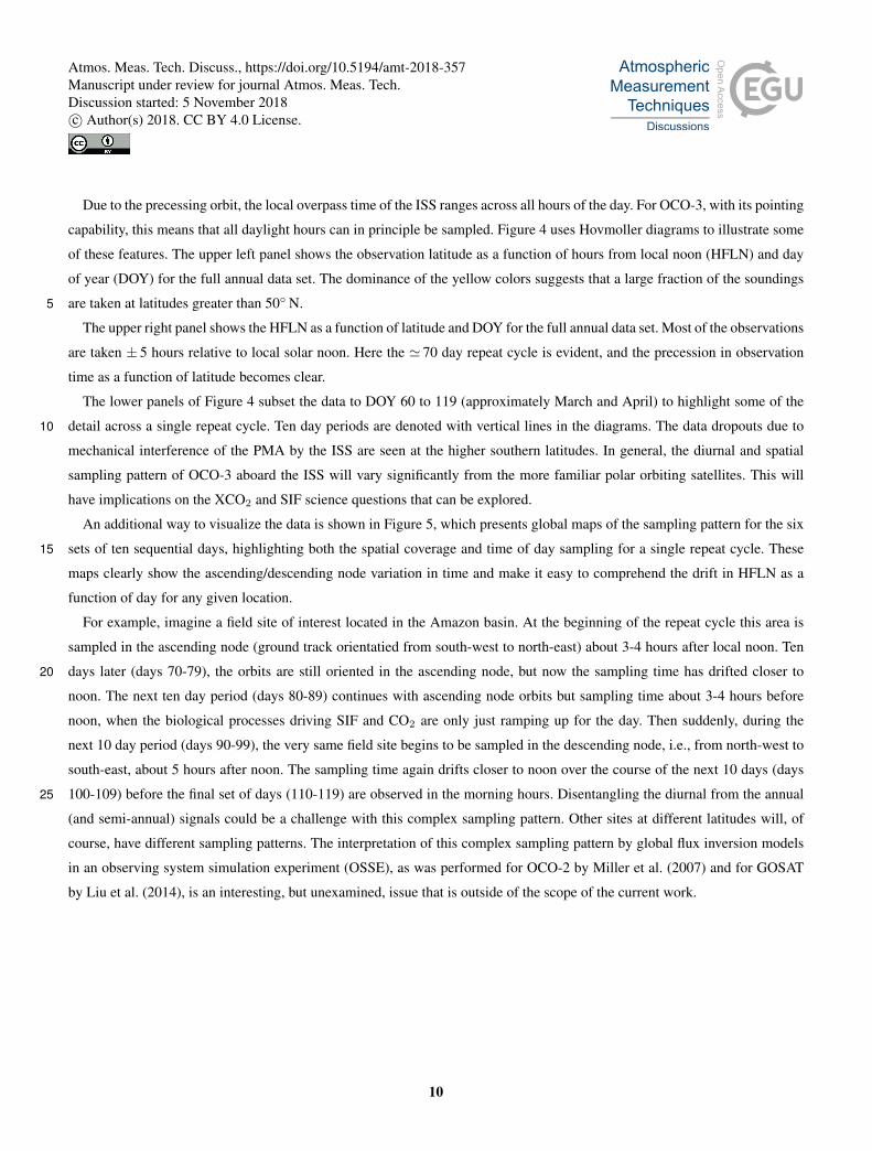
Another way to visualize the spatiotemporal distribution of the data is presented in Figure 3, which shows seasonal sounding

density maps from the simulated data set, binned at 2◦ by 2◦ latitude. Here, and elsewhere in the manuscript, the seasons are de-

fined as December/January/February (DJF), March/April/May (MAM), June/July/August (JJA), and September/October/November

(SON). Here, no prescreening has been applied, and the reduction in spatiotemporal resolution requires inflation of the values

by 240 to get real expected sounding densities. There are just under a million soundings total for the full year, with approx-30

imately 25 soundings in each 2◦ bin over most of the globe per season. Presenting the data in this manner accentuates the

high density of soundings at the orbit inflection points, although the drift in coverage with seasons is muted. The gaps in data

collection so apparent in Figure 2 are no longer observed when the data have been aggregated monthly or seasonally. This has

implications for the spatial and temporal scales of science questions that can be probed with the OCO-3 observations made

from the ISS.35

9


Due to the precessing orbit, the local overpass time of the ISS ranges across all hours of the day. For OCO-3, with its pointing

capability, this means that all daylight hours can in principle be sampled. Figure 4 uses Hovmoller diagrams to illustrate some

of these features. The upper left panel shows the observation latitude as a function of hours from local noon (HFLN) and day

of year (DOY) for the full annual data set. The dominance of the yellow colors suggests that a large fraction of the soundings

are taken at latitudes greater than 50◦ N.5

The upper right panel shows the HFLN as a function of latitude and DOY for the full annual data set. Most of the observations

are taken ± 5 hours relative to local solar noon. Here the ' 70 day repeat cycle is evident, and the precession in observation

time as a function of latitude becomes clear.

The lower panels of Figure 4 subset the data to DOY 60 to 119 (approximately March and April) to highlight some of the

detail across a single repeat cycle. Ten day periods are denoted with vertical lines in the diagrams. The data dropouts due to10

mechanical interference of the PMA by the ISS are seen at the higher southern latitudes. In general, the diurnal and spatial

sampling pattern of OCO-3 aboard the ISS will vary significantly from the more familiar polar orbiting satellites. This will

have implications on the XCO2 and SIF science questions that can be explored.

An additional way to visualize the data is shown in Figure 5, which presents global maps of the sampling pattern for the six

sets of ten sequential days, highlighting both the spatial coverage and time of day sampling for a single repeat cycle. These15

maps clearly show the ascending/descending node variation in time and make it easy to comprehend the drift in HFLN as a

function of day for any given location.

For example, imagine a field site of interest located in the Amazon basin. At the beginning of the repeat cycle this area is

sampled in the ascending node (ground track orientatied from south-west to north-east) about 3-4 hours after local noon. Ten

days later (days 70-79), the orbits are still oriented in the ascending node, but now the sampling time has drifted closer to20

noon. The next ten day period (days 80-89) continues with ascending node orbits but sampling time about 3-4 hours before

noon, when the biological processes driving SIF and CO2 are only just ramping up for the day. Then suddenly, during the

next 10 day period (days 90-99), the very same field site begins to be sampled in the descending node, i.e., from north-west to

south-east, about 5 hours after noon. The sampling time again drifts closer to noon over the course of the next 10 days (days

100-109) before the final set of days (110-119) are observed in the morning hours. Disentangling the diurnal from the annual25

(and semi-annual) signals could be a challenge with this complex sampling pattern. Other sites at different latitudes will, of

course, have different sampling patterns. The interpretation of this complex sampling pattern by global flux inversion models

in an observing system simulation experiment (OSSE), as was performed for OCO-2 by Miller et al. (2007) and for GOSAT

by Liu et al. (2014), is an interesting, but unexamined, issue that is outside of the scope of the current work.

10


Figure 2. Simulated sounding densities for nadir-land (left) and glint-water (right) for the annual (top) and DOY 60-119 (bottom) data sets.

Data are binned in 1 day by 2◦ latitude increments. Values should be inflated by 240 to reflect real expected sounding densities at the full

spatial (8 footprints per frame) and temporal (3 Hz) acquisition rates. To account for the large dynamic range, the density scale has been

truncated at 150, although the extreme high latitudes contains up to 300 soundings per bin in some cases.

3.2 Simulated instrument polarization angle and Stokes coefficients

As unpolarized solar radiation traverses the earth’s atmosphere (twice) prior to incidence upon the OCO instrument, interactions

with particles, e.g., oxygen molecules and aerosols, as well as reflection off the surface, introduce some amount of polarization.

Both the OCO-2 and OCO-3 instruments are sensitive only to radiation that is oriented perpendicular to the long axis of the

11


Figure 3. Seasonal L1b sounding density maps for 2◦ by 2◦ latitude bins. Values should be inflated by 240 to reflect real expected sounding

densities at the full spatial (8 footprints per frame) and temporal (3 Hz) acquisition rates.

spectrometer slits 1. This is critical over strongly polarizing water surfaces, but of lesser concern over land surfaces, which

are only slightly polarizing. In the limit that the axis of accepted and actual polarization are perfectly orthogonal, the intensity

observed by the instrument is identically zero. Although the degree (i.e., amount) of polarization of the reflected sun light

is unknown (although somewhat predictable for water-glint measurements), the polarization angle of any particular sounding,

which is a form of the throughput of the instrument, is a quantity that is calculable from illumination and observing geometries.5

1As noted in (Crisp et al., 2017), the OCO-2 instrument was built erroneously; it was intended to be sensitive only to light parallel to the long axis of the

spectrometer slits. OCO-3 was built in the same manner. This error was mitigated on OCO-2 by yawing the spacecraft in order to maximize the signal over

ocean while simultaneously maintaining sufficient electrical power generated from sunlight on incident on the spacecraft solar panels. For OCO-3, electrical

power comes from the ISS and is therefore a non-issue.

12


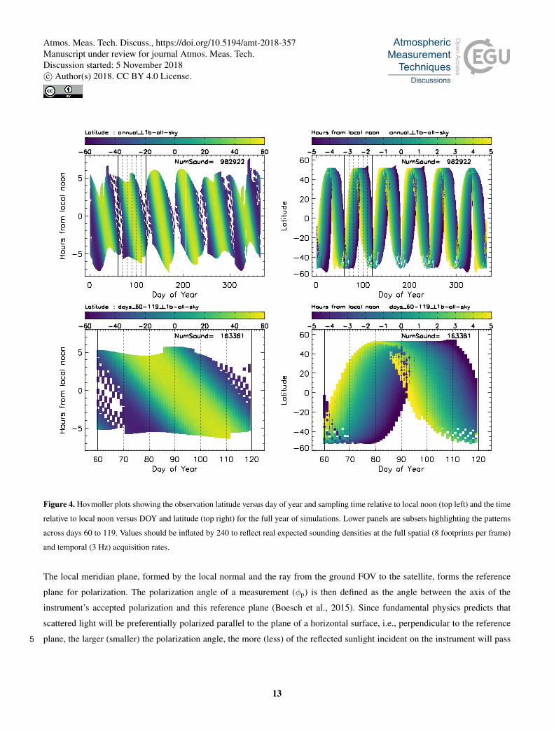
Figure 4. Hovmoller plots showing the observation latitude versus day of year and sampling time relative to local noon (top left) and the time

relative to local noon versus DOY and latitude (top right) for the full year of simulations. Lower panels are subsets highlighting the patterns

across days 60 to 119. Values should be inflated by 240 to reflect real expected sounding densities at the full spatial (8 footprints per frame)

and temporal (3 Hz) acquisition rates.

The local meridian plane, formed by the local normal and the ray from the ground FOV to the satellite, forms the reference

plane for polarization. The polarization angle of a measurement (φp) is then defined as the angle between the axis of the

instrument’s accepted polarization and this reference plane (Boesch et al., 2015). Since fundamental physics predicts that

scattered light will be preferentially polarized parallel to the plane of a horizontal surface, i.e., perpendicular to the reference

plane, the larger (smaller) the polarization angle, the more (less) of the reflected sunlight incident on the instrument will pass5

13


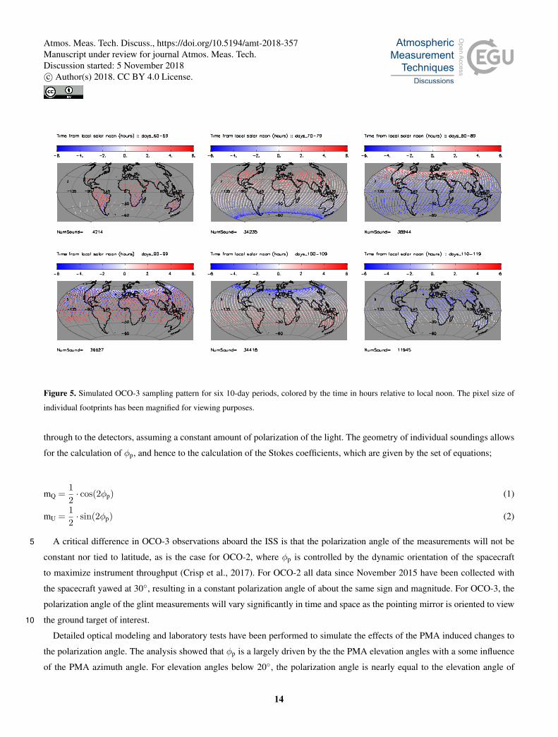
Figure 5. Simulated OCO-3 sampling pattern for six 10-day periods, colored by the time in hours relative to local noon. The pixel size of

individual footprints has been magnified for viewing purposes.

through to the detectors, assuming a constant amount of polarization of the light. The geometry of individual soundings allows

for the calculation of φp, and hence to the calculation of the Stokes coefficients, which are given by the set of equations;

mQ =12· cos(2φp) (1)

mU =12· sin(2φp) (2)

A critical difference in OCO-3 observations aboard the ISS is that the polarization angle of the measurements will not be5

constant nor tied to latitude, as is the case for OCO-2, where φp is controlled by the dynamic orientation of the spacecraft

to maximize instrument throughput (Crisp et al., 2017). For OCO-2 all data since November 2015 have been collected with

the spacecraft yawed at 30◦, resulting in a constant polarization angle of about the same sign and magnitude. For OCO-3, the

polarization angle of the glint measurements will vary significantly in time and space as the pointing mirror is oriented to view

the ground target of interest.10

Detailed optical modeling and laboratory tests have been performed to simulate the effects of the PMA induced changes to

the polarization angle. The analysis showed that φp is a largely driven by the the PMA elevation angles with a some influence

of the PMA azimuth angle. For elevation angles below 20◦, the polarization angle is nearly equal to the elevation angle of

14


the PMA. In the nadir observing mode, the sensitivity to polarization is essentially negligible. However, for all off-nadir

measurements, i.e., glint, transition, target, and snapshot modes, there will be a range of polarization angles, as the elevation

angle of the PMA is adjusted to view the ground target. Ultimately this will have effects on the signal to noise ratios, as will

be discussed in Section 5.1.

3.3 Simulated meteorology, gas and cloud/aerosol fields5

In our simulations, vertical profiles of standard meteorological information needed to calculate realistic radiances were taken

from the National Centers for Environmental Prediction (NCEP) (Saha et al., 2014). The NCEP database has a native spatial

resolution of 2.5◦ latitude by 2.5◦ longitude (10,512 spatial points) with variables given on 17 vertical layers every 6 hours.

For this work, the model was sampled at individual OCO-3 observations, defined by time, latitude, longitude, and surface

elevation, for temperature, humidity, two meter temperature, surface pressure, and winds. The data are interpolated spatially10

and temporally to 26 vertical levels to create "scenes" for every individual OCO-3 sounding.

Vertical values of carbon dioxide for each sounding were sampled from the CarbonTracker 2015 database (CT2015) (Peters

et al., 2007), with updates documented at http://carbontracker.noaa.gov), which has a native spatial resolution of 2.0◦ latitude by

3.0◦ longitude (10,800 spatial points), with CO2 mole fractions given on 25 vertical layers every 3 hours. Data are interpolated

in space and time to match individual OCO-3 soundings. Note that although the ISS ephemeris was taken from 2015, the CT15

database was sampled for 2012. Ultimately this makes no difference to the overall outcomes reported in this paper (which are

not focused on actual carbon cycle science), but it is important to note that the simulations are representative of an earth-like

system, not the actual conditions on Earth at the time of the soundings.

For each individual sounding, a cloud and aerosol profile containing 25 vertical layers was built based on a random selection

from a monthly climatology of CALIOP profiles binned at 2.0◦ latitude by 2.0◦ longitude (16,200 spatial points), as described20

in the OCO simulator document (O’Brien et al., 2009). While these profiles do not capture the diurnal characteristics of cloud

and aerosol fields (as CALIOP, flying in the A-Train, always has the same local overpass time), they are sufficient for this

analysis, which is assessing statistics on monthly or seasonal time scales.

3.4 Simulated land surface model and SIF

A model of the earth’s surface is a critical component for the calculation of reflected solar radiances. For land surfaces, scalar25

Bi-Directional Reflectance Distribution Functions (BRDF) were taken from the MODIS 16-day MCD43B1 product (Schaaf

et al., 2002). For water surfaces, a fully polarized Cox and Munk model with a foam component based on wind speed was used.

Additional details and citations can be found in the CSU simulator ATBD (O’Brien et al., 2009). Realistic estimates of solar

induced chlorophyll fluorescence (SIF) from biological activity were added to the oxygen A-band L1b radiances based on the

implementation of Frankenberg et al. (2012). A static gross primary production (GPP) climatology of Beer et al. (2010), which30

is a mean monthly climatology based on the 18 IGBP surface types at 0.5◦ by 0.5◦ latitude and longitude resolution, is scaled

to a daily average SIF value using the empirical scaling factor of Frankenberg et al. (2011). Daily average SIF is converted

to instantaneous SIF via scaling by the instantaneous solar insolation relative to the average for that day and location. The

15


wavelength dependence is a double Gaussian function as given in Frankenberg et al. (2012). Overall, this provides values of

SIF that are representative in time (seasonal and diurnal cycle) and space (as a function of latitude and local plant physiology).

It is worth noting that the use of the static GPP climatology does not allow for interannual variability, but this has no effect on

the single year of simulated data presented here.

3.5 Simulated L1b radiances5

Radiances, as would be observed by the OCO-3 instrument in space, are calculated using the same forward model (FM) that

has previously been employed for GOSAT and OCO-2 simulation studies, e.g., O’Dell et al. (2012). The FM consists of a

atmospheric model, surface model, instrument model, solar model, and radiative transfer model.

The solar spectrum is comprised of two parts; a pseudo-transmittance spectrum (Toon et al., 1999) and a solar continuum

spectrum (Thuillier et al., 2003), used to produce a high-resolution, absolutely-calibrated input solar spectrum for the for-10

ward model (Boesch et al., 2015). For this work, the gas absorption coefficients, i.e., spectroscopy, of the current operational

OCO-2 B8 L2 algorithm, ABSCO v5.0.0, were used. The instrument model, which includes the instrument line shapes (ILS),

radiometric characteristics, polarization sensitivity, and noise specifications, were taken from the OCO-3 thermal vacuum tests

performed in September 2016. Noise was applied to the calculated radiances via the same model used for OCO-2, as de-

scribed in Rosenberg et al. (2017). The radiative transfer calculation accurately accounts for multiple scattering from clouds15

and aerosols as well as polarization, as described in O’Brien et al. (2009) and references therein.

4 Level 2 preprocessors and full physics retrieval algorithms

The primary data products for OCO-2 and OCO-3 are the column-averaged dry-air mole fraction of CO2 (XCO2) and the solar

induced chlorophyll fluorescence (SIF), both of which can be used to help constrain the global carbon cycle, e.g. Eldering

et al. (2017b); Sun et al. (2017). For this work, the simulated L1b radiances were analyzed with the same tools used in OCO-220

operational data processing, as described in Section 4 of Eldering et al. (2017a). These steps include prescreening, L2 retrievals,

quality screening and the application of a bias correction for XCO2. This section briefly discusses each of the components as

it relates specifically to the OCO-3 simulations. Relevant citations containing the full details are provided.

4.1 Preprocessors

Cloud screening was performed using only the A-Band Preprocessor (ABP), as described in Taylor et al. (2016). The ABP25

identifies cloud contaminated soundings primarily via a threshold on the difference in retrieved and prior surface pressure

in the Oxygen-A band, typically ± 25 hPa. Although operational OCO-2 data also utilizes a weak filter on the ratio of CO2

retrieved independently in the strong and weak CO2 bands by the IMAP-DOAS Preprocessor (IDP), we did not implement

this filter for cloud screening. The IDP CO2 and H2O ratios were however used for post L2 retrieval quality filtering and bias

correction. In addition IDP performs a retrieval of SIF, which is used as a prior for the full physics L2 SIF retrieval. After some30

additional post processing, such as removing a zero level offset (ZLO), the IDP SIF becomes the formal LiteSIF product that is

16


available on the NASA DISC. Both preprocessors neglect scattering in the atmosphere (except Rayleigh scattering is included

in ABP), making them computationally very efficient.

4.2 Full physics retrieval algorithm for XCO2 and SIF

The soundings that were identified as clear by the ABP cloud flag were then run thru the OCO-2 B8 operational retrieval

algorithm. The algorithm was first described in Bösch et al. (2006) and Connor et al. (2008) prior to the failed launch of5

OCO-1 in February 2009, and was later applied to GOSAT as described in O’Dell et al. (2012). Recent updates and a complete

description of the modern B8 version of the algorithm can be found in Boesch et al. (2015) and O’Dell et al. (2018).

In summary, the algorithm is an optimal estimation retrieval with a prior that minimizes radiance residuals, i.e., chi-squared,

to maximize the a posterior probability. The solution is solved on 20 vertical levels, with the state vector containing CO2 dry

air mole fraction, aerosol parameters, surface albedo, wind speed, water vapor, and a temperature scaling factor. The high10

spectral resolution measurements of top of the atmosphere reflected radiances measured by sensors such as GOSAT, OCO-2,

or OCO-3 serve as the primary source of information in the retrieval. The measurements are coupled with an a priori state

of the atmosphere in order to constrain the inversion. Within the L2 retrieval, modeled spectra are generated by a radiative

transfer code as described in O’Dell et al. (2012) and Boesch et al. (2015). Although they share many components, the L2 code

base differs slightly from the RT FM used in the generation of the L1b radiances, thus creating a realistic error source in the15

simulation exercise, i.e., imperfect radiative transfer.

4.3 Filtering and bias correction approach

The NASA operational procedure for both OCO-2 and GOSAT applies a quality filtering (QF) and bias correction (BC) process

to the retrieved XCO2 (O’Dell et al., 2018). Correlations between variables and XCO2 error variability are quantified and used

to develop the filtering thresholds and linear bias correction equations. The quality filtering is designed to remove soundings20

with anomalous XCO2 values relative to other soundings in close proximity, making use of the assumption that real variations

in XCO2 are quite small (<1 ppm) on small scales (< 100 km). Some form of "truth" metric, or truth proxy, is required with

which to calculate an "error" in XCO2. For operational OCO-2 data, several forms of a truth proxy are used, as detailed in

Section 4.1 of O’Dell et al. (2018).

A similar treatment was applied to the OCO-3 simulation dataset. However, with simulations it was possible to use the actual25

true XCO2 as the truth proxy in the QF and BC procedures. There are both advantages and disadvantages to the circularity

imposed by knowing the true values of the atmospheric state. In this case, we expect that the use of the truth data will result in

an overly optimistic QF and BC.

At its completion, the QF/BC procedure assigns to every sounding a binary flag indicating good/bad quality, as well as a BC

value (in units ppm). The operational OCO-2 BC equation contains three components; a correction based on retrieval variables30

(parametric), a correction for inter-footprint dependence and a global bias, each calculated separately for land (combined nadir

and glint) and ocean-glint. For the OCO-3 simulations the inter-footprint bias is not needed since only a single footprint per

17


frame was calculated. Explicit results from the procedure as performed on the OCO-3 simulations are given in Sections 5.3

and 5.4.

5 Results

This section discusses characteristics of the L1b radiances, performance of the preprocessors, and application of the quality

filter and bias correction methodology before presenting the L2 XCO2 results. In addition, we provide a brief analysis of the5

SIF determined by the IDP retrieval. Table 1 summarizes the number of soundings in the simulated data set at each stage of the

analysis, broken out by nadir-land and glint-water observations.

5.1 Simulated L1b radiance characteristics

At a gross level, the characteristics of the simulated OCO-3 radiances are very similar to those from real OCO-2 measurements.

The high resolution spectra for OCO-3 (not shown) exhibit the expected absorption features that allow for cloud and aerosol10

screening, and the retrieval of surface pressure and SIF (from the O2 A-band) and XCO2 (from the weak and strong CO2

bands).

However, some differences are expected between the two sensors in both measured signal and instrument noise due to

the addition of the PMA and calibration characteristics of the spectrometers, e.g., dark noise, stray light and ILS. Optical

inefficiencies in the OCO -3 PMA will reduce the transmission of light by about 17% in the O2 A-band, and 7% and 5% in15

the weak and strong CO2 bands, respectively. To compensate for the effects of the PMA, the instrument aperture of the O2

A-band was increased. When all of the optical elements and instrument changes are considered, the O2 A-band transmission

of OCO-3 will be about 95% of OCO-2, while the weak and strong CO2 bands will have 75% of the transmission of OCO-2,

thus reducing the observed signal for the same scene.

The instrument calibration parameters for the OCO-3 simulations reported here were taken from results of the September20

2016 pre-launch thermal vacuum testing (TVAC), which was performed using an early version of the instrument telescope

and without the PMA installed. The noise coefficients were adjusted post-hoc to account for the reduced optical throughput

caused by the PMA. Although the final round of pre-launch TVAC calibration was completed in May 2018, the results were

still not available at the time of writing. However, based on preliminary analysis, the updated instrument characteristics are not

expected to change at a level that would greatly effect the results presented here.25

A key characteristic of the radiances measured by satellite sensors is the SNR, which effectively determines the information

content of the measurements, thereby controlling the precision of the retrieval estimates of XCO2 and SIF. The signal for each

band is calculated from continuum level radiances, using the ten channels with the highest values, after filtering for outliers that

occasionally exist due to cosmic rays or some other random electronic anomoly. The OCO noise model combines contributions

from a constant background (dark noise) term and a photon (shot noise) term, the later of which is proportional to the square30

root of the radiance (Rosenberg et al., 2017).

18


Figure 6 compares the OCO-2 SNR calculated from the operational noise model (solid traces) against OCO-3 (dashed traces)

versus a measure of the surface brightness (the albedo scaled by the cosine of the solar zenith angle, A · cos(SZA)). The left

panel displays the SNR of each spectral band for both sensors, while the right panel shows the ratio of the two sensor’s SNR

per spectral band. This data demonstrates that the only situation in which OCO-3 has a higher SNR than OCO-2 (values >1.0

on the right panel) is in the O2 A-band for A · cos(SZA) & 0.15. This typically occurs over very bright deserts and during5

glint-water measurements when the sun is low in the sky. It is worth noting that the O2 A-band is used primarily for cloud and

aerosol detection and for the L2 FP surface pressure retrieval as well as for SIF.

In both of the weak and strong CO2 bands (green and red, respectively, in the figure), OCO-3 always has a significantly lower

SNR than OCO-2. This reduced SNR can be attributed to both increased noise due to the use of noisier instrument detectors

that were spare parts from the rebuild of the OCO-2 instrument, and to decreased signal incurred by the use of the PMA, a10

polarizer in the telescope, and a larger center obscuration in the entrance optics.

The overall SNR differences are captured in the histograms of Figure 7, which compare the OCO-3 simulations with the real

SNR for operational OCO-2 B8 measurements acquired in 2016. The operational OCO-2 data has been down selected to include

only a single footprint and one sounding every 10 seconds to provide a fairer comparison against the OCO-3 simulations. Both

data sets have been screened using the L2 FP quality flags, which were introduced in Section 4.3, and will be discussed in more15

detail in Section 5.3. At a gross level, the data look reasonably similar, although a few key distinctions stand out, particularly

that the slightly brighter OCO-3 O2 A-band is primarily due to a long tail of high values for glint-water soundings. The OCO-3

weak CO2 band exhibits a substantially lower SNR for glint-water compared to OCO-2, while the strong CO2 band tends to

be also lower than OCO-2. These figures show that the OCO-3 data will include less data with SNR values over 600, and more

data with SNR between 200 and 400. Previous OCO-2 studies and experience with the real data show that an SNR of 20020

is sufficient to achieve the desired precision of the retrieval algorithm. As will be shown in Sections 5.5 and 5.6, the L2 FP

retrieval still provides good estimates of XCO2 and SIF on this set of OCO-3 simulated radiances, even with the lower SNR

values.

Maps comparing the simulated OCO-3 SNR to the operational B8 OCO-2 data for each spectral band are shown in Figure 8

for the month of April. Qualitatively, the overall patterns agree quite well, although the difference in latitudinal coverage from25

the two spacecraft is noteworthy. We also note that a higher fraction of the soundings that converge in the L2 FP retrieval

are assigned a good quality filter in the OCO-3 simulations (approximately 70%), versus only about 40% for real OCO-2 B8

data. This is likely driven by deficiencies in the simulation setup, such as lack of a Southern Atlantic Anomaly model, and a

parameterized cloud and aerosol scheme in the L1b simulations that lacks full realism. We expect that real on-orbit OCO-3

good quality sounding fractions will in reality be closer to the OCO-2 values.30

For both sensors, the highest SNR’s are obtained over un-vegetated (bright) land, and for glint-water when the sun is low in

the sky, producing a strong specular reflection. The lowest values of SNR occur when when the sun is high in the sky, and for

vegetated (dark) land surfaces at higher latitudes. As with OCO-2, the weak CO2 band displays the highest SNR values, while

the O2 A-band and strong CO2 bands have lower but comparable SNRs.

19


A final glimpse of the SNR characteristics are shown in Figures 9 and 10, which compare the SNR dependence on lati-

tude and SZA for both sensors. The restriction of OCO-3 to latitudes less than approximately 54◦ is pronounced, especially

for the glint-water soundings, when comparing to the wider latitudinal distribution obtained from OCO-2. This is simply a

consequence of the ISS precessing orbit versus the polar orbit of OCO-2. On the other hand, the OCO-3 measurements span

SZA’s from approximately 85 to 0◦, while OCO-2 measurements are limited to a minimum SZA of approximately 20◦ in the5

subtropics and larger than 30◦ above 40◦ latitude. As was demonstrated previously in the histogram plots (Figure 7, we again

see here that for nadir-land the OCO-3 SNR values tend to be lower for OCO-3 compared to OCO-2 in all spectral bands,

with the exception of a few high O2 A-band SNRs around 20◦ latitude which correspond to the Sahara desert. For glint-water

soundings, there is a population of very high SNR values (> 800) spanning the full latitudinal space, at SZA around 60◦ due

to the very bright specular glint spot achieved under these conditions.10

While real on-orbit SNR characteristics will likely differ somewhat from those shown here, these simulations suggest that the

instrument has been well built and well calibrated and should provide SNR that meets the mission requirements. In addition, due

to the nature of the precessing orbit of the ISS, we expect that the SNR distribution, which fundamentally drives the information

content in the L2 FP retrievals, will not be tied to latitude in the same way that it is for OCO-2. This has implications as to the

spatial patters of good quality XCO2 and SIF retrievals, as will be discussed in the following sections.15

20


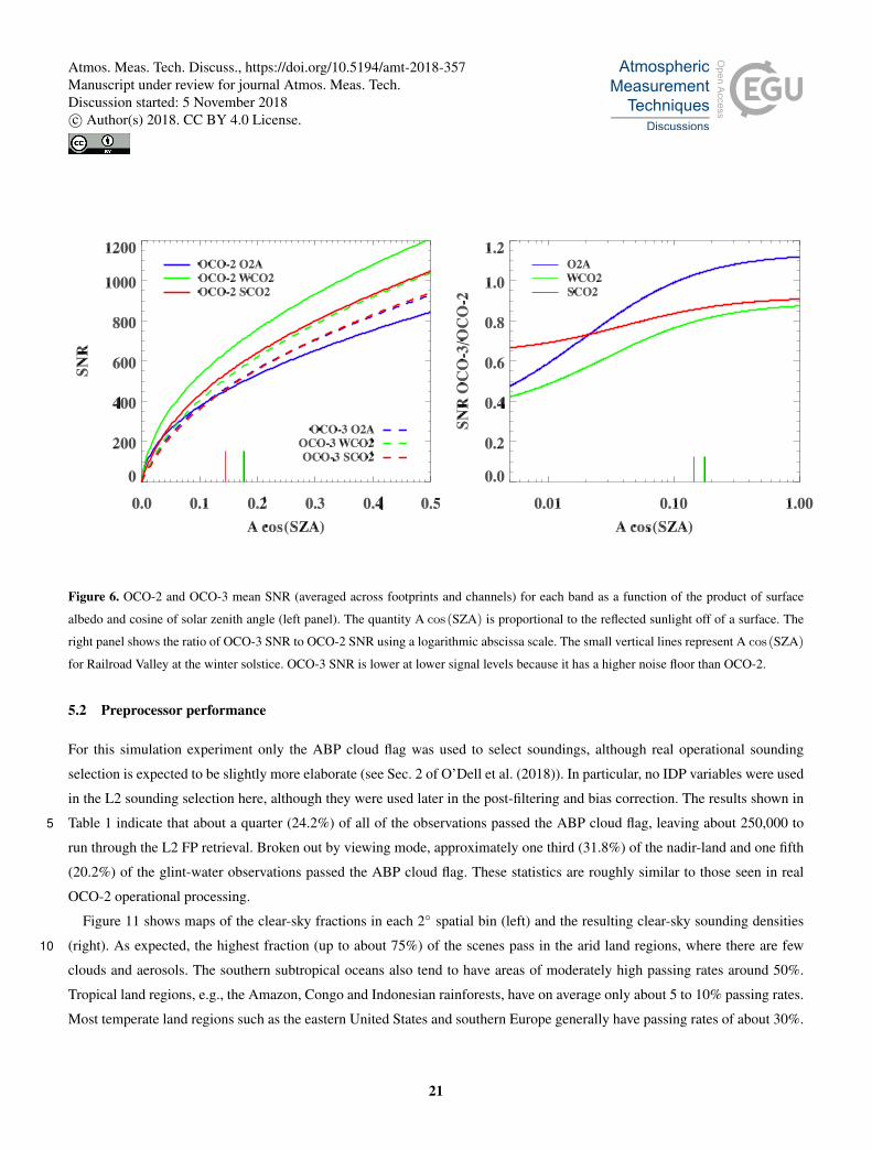
Figure 6. OCO-2 and OCO-3 mean SNR (averaged across footprints and channels) for each band as a function of the product of surface

albedo and cosine of solar zenith angle (left panel). The quantity A cos(SZA) is proportional to the reflected sunlight off of a surface. The

right panel shows the ratio of OCO-3 SNR to OCO-2 SNR using a logarithmic abscissa scale. The small vertical lines represent A cos(SZA)

for Railroad Valley at the winter solstice. OCO-3 SNR is lower at lower signal levels because it has a higher noise floor than OCO-2.

5.2 Preprocessor performance

For this simulation experiment only the ABP cloud flag was used to select soundings, although real operational sounding

selection is expected to be slightly more elaborate (see Sec. 2 of O’Dell et al. (2018)). In particular, no IDP variables were used

in the L2 sounding selection here, although they were used later in the post-filtering and bias correction. The results shown in

Table 1 indicate that about a quarter (24.2%) of all of the observations passed the ABP cloud flag, leaving about 250,000 to5

run through the L2 FP retrieval. Broken out by viewing mode, approximately one third (31.8%) of the nadir-land and one fifth

(20.2%) of the glint-water observations passed the ABP cloud flag. These statistics are roughly similar to those seen in real

OCO-2 operational processing.

Figure 11 shows maps of the clear-sky fractions in each 2◦ spatial bin (left) and the resulting clear-sky sounding densities

(right). As expected, the highest fraction (up to about 75%) of the scenes pass in the arid land regions, where there are few10

clouds and aerosols. The southern subtropical oceans also tend to have areas of moderately high passing rates around 50%.

Tropical land regions, e.g., the Amazon, Congo and Indonesian rainforests, have on average only about 5 to 10% passing rates.

Most temperate land regions such as the eastern United States and southern Europe generally have passing rates of about 30%.

21


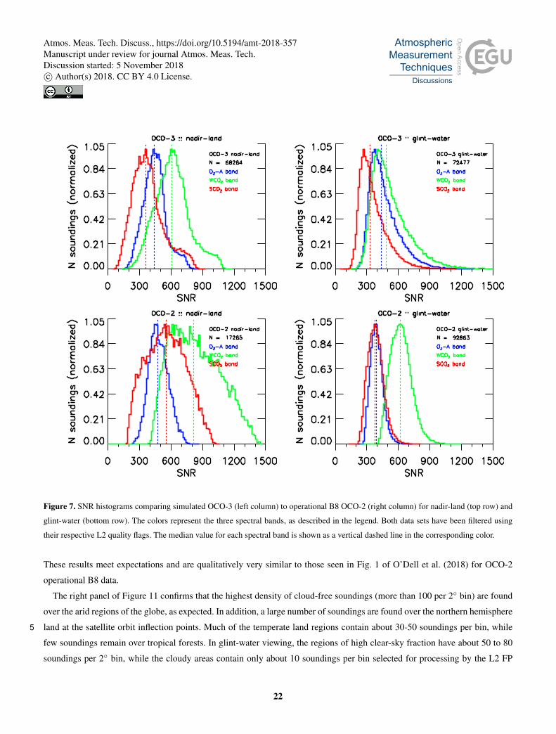
Figure 7. SNR histograms comparing simulated OCO-3 (left column) to operational B8 OCO-2 (right column) for nadir-land (top row) and

glint-water (bottom row). The colors represent the three spectral bands, as described in the legend. Both data sets have been filtered using

their respective L2 quality flags. The median value for each spectral band is shown as a vertical dashed line in the corresponding color.

These results meet expectations and are qualitatively very similar to those seen in Fig. 1 of O’Dell et al. (2018) for OCO-2

operational B8 data.

The right panel of Figure 11 confirms that the highest density of cloud-free soundings (more than 100 per 2◦ bin) are found

over the arid regions of the globe, as expected. In addition, a large number of soundings are found over the northern hemisphere

land at the satellite orbit inflection points. Much of the temperate land regions contain about 30-50 soundings per bin, while5

few soundings remain over tropical forests. In glint-water viewing, the regions of high clear-sky fraction have about 50 to 80

soundings per 2◦ bin, while the cloudy areas contain only about 10 soundings per bin selected for processing by the L2 FP

22


retrieval. Recall that on-orbit OCO-3 sounding densities will be about 240 times greater due to the reduced spatiotemporal

sampling used in this simulation set.

23


5.3 Application of XCO2 quality filter

The L2 FP retrieval algorithm described in Section 4.2 was applied to the cloud screened set of soundings, and then, as with

operational OCO-2 data, a set of post-processing filters were implemented to determine the binary XCO2 quality flags (QF).

Details of the methodology are documented in O’Dell et al. (2018). Here, the true XCO2 for each sounding was used as the

truth metric to assess residual biases and errors. This provides perhaps an overly optimistic interpretation of the results, and5

should be considered an upper limit on the actual performance expected from the real system.

Explicit values of the QF thresholds determined for the OCO-3 simulations are presented in Tables 2 and 3. The QF method-

ology was applied independently to the nadir-land and glint-water scenes, as is done with real OCO-2 data. Eleven variables

were used to form the QF for nadir-land, while nine were used for glint-water. Not surprisingly, many of the same variables are

selected for quality filtering the OCO-3 simulations as were used in the operational OCO-2 procedure. See Figures 10 and 1110

of O’Dell et al. (2018). Approximately 70% of the soundings that converged in L2 FP were assigned a good quality flag.

The quality filtering process had similar impacts on data volume across all months (not shown). On average, global data

densities of good QF soundings in the simulations were 11,000 to 12,000 soundings per month, or 33,000 to 36,000 per season.

When using the full spatiotemporal resolution, this translates to approximately 2.5 million soundings per month (7.5 million

per season), similar to the density of OCO-2 B8 data.15

Figure 12 shows seasonal plots of the fraction (left column) and number (right column) of soundings passing the quality

filters for each season (DJF, MAM, JJA, SON), binned in 4◦ degree lat/lon bins. The spatial patterns are useful, but the absolute

numbers need to be inflated by 240 to reflect actual predicted on-orbit throughput. These maps can be compared with those

shown in Figure 12 of O’Dell et al. (2018).

In general, the QF throughputs for glint-water are quite high (>70%) in the tropics and subtropics (<30◦ latitude), and display20

very little seasonal cycle. The QF throughput is persistently low for glint-water observations at the extreme latitudes. The QF

throughputs are more varied for nadir-land observations, and a modest seasonal cycle is seen for some regions. But overall, the

results look qualitatively similar to those from OCO-2 for the B8 operational data set, and demonstrate that the methodology

is a robust procedure.

24


5.4 Bias correction of XCO2

The final bias correction (BC) incorporates four of the QF variables for nadir-land and three for glint-water as shown in Table 4.

There are notable similarities and differences in the selected variables when comparing between the OCO-3 simulations and

real OCO-2 data. See Section 4.3.1 in O’Dell et al. (2018).

Figure 13 illustrates how the final BC parameters for land affect the XCO2 error. Each panel shows median binned values of5

the XCO2 error (retrieved minus true in ppm) versus a particular retrieval variable shown by the heavy black dots. Also shown

are the range in XCO2 error (thin vertical bars) and the least squares linear fit (thin dashed line). To provide context, the relative

histogram of points is shown in the background by the shaded grey region. The slope of the fit, the standard deviation of the

XCO2 error post BC, and the percent of the variance explained by this variable are given in the legend. The original standard

deviation is shown in the upper left panel for reference.10

For land, 25% of the variance is explained by the L2 dP (retrieved surface pressure minus a priori), while another 15% is

explained by the combined retrieved AOD from dust and sea salt aerosols. An additional 3% and 2% are explained by the L2

fine mode AOD and the water vapor scaling factor, respectively. We believe that a minor indexing bug found in the meteorology

is responsible for the reliance on water vapor. The final reduction in XCO2 error is shown in Table 6, which gives the standard

deviations (sigma) in the retrieved XCO2 with and without QF and BC. For land, sigma was reduced from 1.88 ppm to 0.85 ppm15

after application of both QF and BC.

Figure 14 is similar to Figure 13, but for the glint-water scenes. Here, 18% of the variance in XCO2 error is explained by

the IDP CO2 ratio, while another 16% is explained by the ABP dP. An additional 7% is explained by the L2 dP. As seen in

Table 6, sigma was reduced from 2.15 ppm to 0.52 ppm for glint water soundings after application of both QF and BC.

Spatial seasonal maps of the total bias correction (in units ppm) are shown in Figure 15. Although the results are qualitatively20

different from those seen for operational OCO-2 B8 data presented in O’Dell et al. (2018), this follows expectations in that

here we are working with simulated data which is more internally consistent then real data, especially with respect to ABSCO

and meteorology. These results underscore the conclusion that even given nearly perfect alignment of the retrieval model with

the truth, there are still retrieval errors that induce biases and scatter into the estimates of XCO2. This is particularly true of

aerosols, which are a continued known source of trouble in virtually all retrievals of greenhouse gases from space, e.g., (Aben25

et al., 2007; Butz et al., 2009).

25


5.5 Retrieved XCO2 characteristics after filtering and bias correction

One of the objectives of this study was to analyze the error on the retrieved XCO2 from OCO-3. Here the “actual” error is

given as the retrieved value minus the known truth (after applying the averaging kernel correction), and is denoted ∆XCO2.

The “predicted” error is an L2 FP retrieval state vector parameter that provides the theoretical error due to the combination

of measurement noise plus smoothing and interference errors, as discussed in Boesch et al. (2015). The actual errors in the5

simulated framework are expected to be substantially lower than those seen in OCO-2 operational data, while the predicted

errors should be roughly equivalent due to use of similar instrument model and retrieval algorithm.

As demonstrated in Figure 16, which shows the histograms of ∆XCO2 for nadir-land and glint-water data separately,

∆XCO2 is small and effectively corrected by the filtering and bias correction process on an annual average basis. Overall,

QF/BC reduces the median ∆XCO2 bias from -0.12 to -0.02 ppm for land soundings and from 0.23 to -0.09 ppm for glint-10

water soundings. The histograms indicate that the filtering process identifies a significant population of glint-water soundings

with large negative biases up to about -12 ppm.

The seasonal spatial distributions of ∆XCO2 are shown in the maps of Figure 17. These can be compared to Figure 19 of

O’Dell et al. (2018). While the qualitative patterns of actual XCO2 errors are quite different between OCO-2 B8 and simulated

OCO-3 data, note that the dynamic range of the scale is much lower for OCO-3 (±1 ppm) compared to OCO-2 (±3 ppm).15

Again, this follows expectations since the truth proxy for the simulations is the actual truth, while that metric is not available

in the real world.

For the OCO-3 simulations, after QF/BC have been applied, the errors are largely uncorrelated with any geophysical or

retrieval parameters. Specifically, we used the glint-water soundings to check for correlation of both the raw and BC XCO2

data against latitude, solar zenith angle, polarization angle, SNR (per spectral band), and the true aerosol optical depth. The20

results are summarized in Table 5. It is worth noting that the true AOD was not used as a bias fitting parameter, yet there is

a high reduction in the correlation with ∆XCO2. The very small slopes, offsets and linear correlation coefficients that remain

after application of the QF/BC indicates that remaining errors in the XCO2 are likely driven by retrieval errors such as the

aerosol parameterization (Nelson et al., 2016).

Shown in Figure 18 are the OCO-3 actual (∆XCO2) versus the L2 FP retrieval predicted XCO2 errors comparing the25

unfiltered raw, the filtered raw and the filtered and bias corrected data. There is a huge improvement in the performance after

filtering is applied. Additional improvements are achieved by application of the bias correction. Results fall nearly on the one-

to-one line, with some exception for nadir-land soundings when the predicted error falls below about 0.7 ppm, in which case

the actual error is larger than theory. Overall, these results provide evidence that the filtering and bias correction methodology

is a robust procedure that performs according to theory given a (nearly) perfect truth metric.30

26


5.6 Retrieved SIF characteristics

Similar to the analysis of XCO2 in the previous section, here we present the IDP SIF relative to the true values and examine

both the actual and predicted errors. In order to calculate the “actual” SIF error (retrieved - true), the L1b truth values, which

are calculated at 755 nm in the simulator code, were first wavelength shifted to match the IDP retrieved values at 758.65 nm

and 769.95 nm. Note that these IDP channel values denote the center points of the retrieval ranges but are labeled as 757 nm5

and 771 nm throughout the code and analysis for historical purposes as reported in Section 2.2 of Sun et al. (2018). For brevity,

we only show results for the 757 nm band, although there is no reason to expect a significant difference in performance in the

771 nm band.

The retrieval of SIF from space is highly sensitive to measurement error, i.e., instrument noise (Frankenberg et al., 2014). It

is therefore a common practice to aggregate some number of soundings, N, in order to minimize the random noise. Since these10

simulations have spatiotemporal sampling of 1/240 of the real expected value, we “noise-corrected” our results by scaling the

noise as;

SIF′ = SIF +noise√

240, (3)

where SIF represents the retrieved values using noiseless radiances, and noise is calculated by differencing the with- and

without- instrument noise retrievals.15

Unlike with XCO2, the retrieval of SIF using the solar Fraunhofer lines is not highly sensitive to cloud and aerosol contam-

ination (Frankenberg et al., 2012) We therefore did not apply any strict prescreening or L2 quality flagging prior to running

the IDP retrieval on the L1b files. Although IDP can in principle retrieve SIF over water, glint-water soundings were ignored

since the L1b simulator assumes zero SIF in these cases. Out of the 337,000 total land soundings approximately 12% of the

IDP retrievals failed altogether (identified by way of fill values in the output).20

We then applied a post processing quality filter on the approximately 300,000 successful nadir-land soundings, which in-

cluded removal of scenes with SZA > 70, for which the actual SIF error became very large. We also removed 49 soundings

where the predicted retrieval noise as a function of the continuum level radiance fell well outside a smooth fitting criteria. For

unknown reason these small number of soundings had very large actual SIF errors. After application of the filtering criteria,

approximately 264,000 land soundings (88% of the successful soundings 2) remained in the annual data set.25

The top row of Figure 19 shows maps of the true (left) and IDP retrieved SIF (right) for the 757 nm band for the JJA season,

when the northern hemisphere land photosynthetic activity is at its annual maximum. The units are expressed in radiance space

as Watts-per-square-meter-per-micron-per-steradian (W/m2/µm/sr). SIF typically comprises at the maximum about 1 to 2%

of the total radiance measured at the top of the atmosphere by satellite sensors (Frankenberg et al., 2012). At a gross scale,

the true and retrieved values show the expected patterns, with SIF up to about 1.2 W/m2/µm/sr in densely vegetated tropical30

regions, when aggregated to 1◦ by 1◦ bins, and (near) zero SIF over barren deserts, high mountains and high latitudes.

2It is coincidence that both the fraction of soundings that failed the IDP retrieval and the number that were flagged by our post processing filter is 12%.

27


Although they appear qualitatively similar, the absolute difference in true and retrieved values suggests that the IDP tends to

underestimate SIF. This is particularly so for higher fluorescing areas, as seen in the middle left of Figure 19. To better quantify

the differences in the retrieved and true values, a fractional difference was calculated after masking out the soundings with true

SIF less than 0.2 W/m2/µm/sr (to avoid the intractable math of the ratio of two numbers close to zero). As seen in the middle

right panel, the median fractional differences in SIF is -9% for this subset of the data, with individual soundings having outliers5

as large as -240%. The bottom row of panels shows the correlation between the true and retrieved values for the JJA data, with

and without the true SIF < 0.2 W/m2/µm/sr. The Pearson linear correlation coefficients are very close to 1, indicating that the

retrieval of SIF from the IDP is expected to perform well for the OCO-3 instrument, as has already been shown for operational

OCO-2 data (Sun et al., 2017, 2018).

The comparison between the “actual” (retrieved minus true) and “predicted” SIF error are shown in Figure 20. Here we10

show both the unfiltered, i.e., no quality flag applied, and filtered annual data sets. When the retrieval predicted error is

above approximately 0.25 W/m2/µm/sr the actual error is in very close agreement for the filtered data. Below predicted

error of '0.25 W/m2/µm/sr, the filtered data set still tends to have a slightly larger value of actual error. For predicted error

< 0.25 W/m2/µm/sr the actual error becomes quite large in the unfiltered data set.

A comparison of the single sounding SIF precision between the OCO-3 simulations and the operational B8 OCO-2 data15

is given in Figure 21 for both the 757 nm and 771 nm windows. For both instruments, the precision is an increasing function

of the continuum level radiance, as explained in Section 3.1 of Frankenberg et al. (2014) in association with Figure 8. The

darker the scene, the better the precision, due to decreasing noise in the Fraunhofer lines. Overall, both instruments have better

precision at the shorter wavelength channel. This analysis suggests that OCO-3 SIF precision will be 10-20% worse than for

OCO-2, which may be directly ascribable to the noisier instrument detectors. More research and analysis on IDP SIF using20

real on-orbit measurements will be needed to determine answers.

28


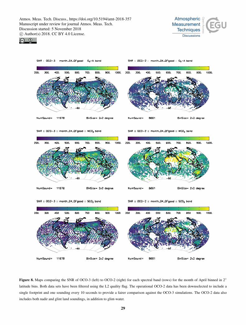
Figure 8. Maps comparing the SNR of OCO-3 (left) to OCO-2 (right) for each spectral band (rows) for the month of April binned in 2◦

latitude bins. Both data sets have been filtered using the L2 quality flag. The operational OCO-2 data has been downselected to include a

single footprint and one sounding every 10 seconds to provide a fairer comparison against the OCO-3 simulations. The OCO-2 data also

includes both nadir and glint land soundings, in addition to glint-water.

29


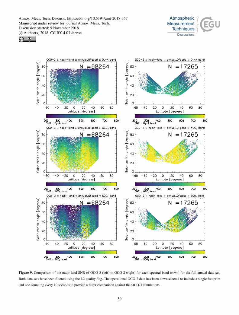
Figure 9. Comparison of the nadir-land SNR of OCO-3 (left) to OCO-2 (right) for each spectral band (rows) for the full annual data set.

Both data sets have been filtered using the L2 quality flag. The operational OCO-2 data has been downselected to include a single footprint

and one sounding every 10 seconds to provide a fairer comparison against the OCO-3 simulations.

30


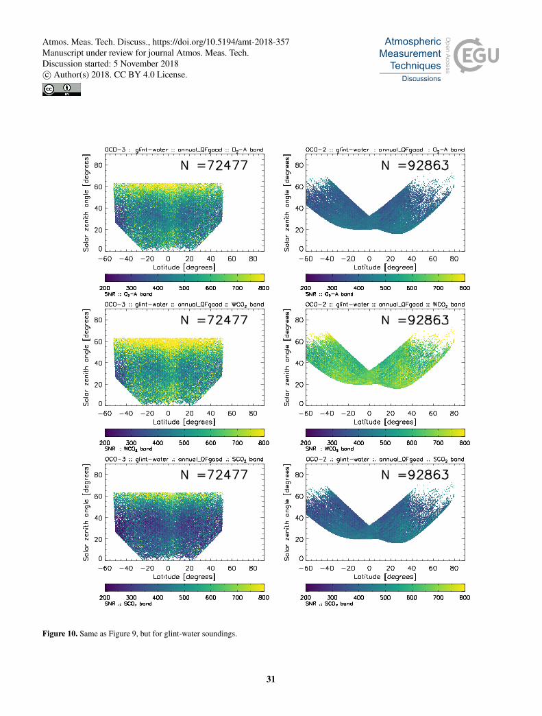
Figure 10. Same as Figure 9, but for glint-water soundings.

31


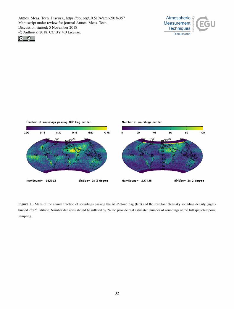
Figure 11. Maps of the annual fraction of soundings passing the ABP cloud flag (left) and the resultant clear-sky sounding density (right)

binned 2◦x2◦ latitude. Number densities should be inflated by 240 to provide real estimated number of soundings at the full spatiotemporal

sampling.

32


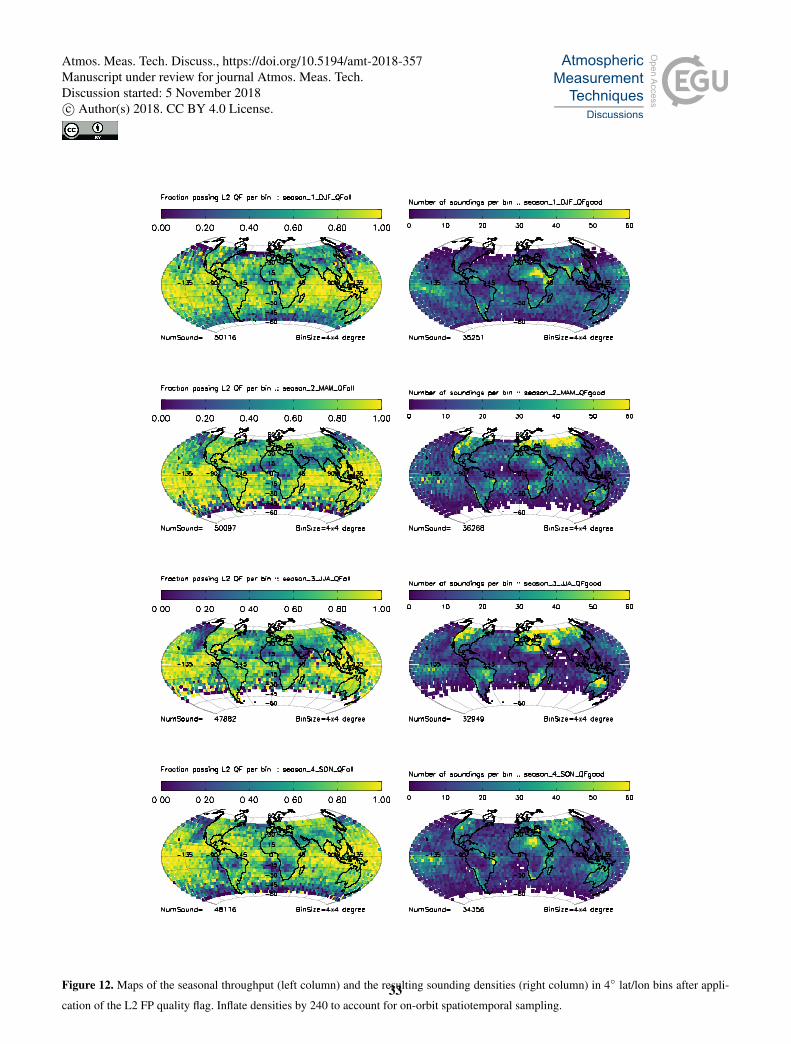
Figure 12. Maps of the seasonal throughput (left column) and the resulting sounding densities (right column) in 4◦ lat/lon bins after appli-

cation of the L2 FP quality flag. Inflate densities by 240 to account for on-orbit spatiotemporal sampling.33


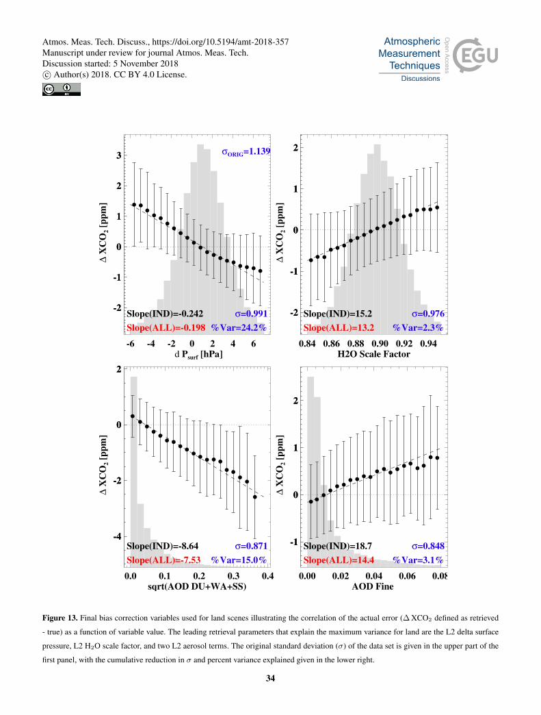
-6 -4 -2 0 2 4 6d Psurf [hPa]

-2

-1

0

1

2

3

∆ X

CO

2 [

pp

m]

-2

-1

0

1

2

3 σORIG=1.139

σ=0.991

%Var=24.2%

Slope(IND)=-0.242

Slope(ALL)=-0.198

0.84 0.86 0.88 0.90 0.92 0.94H2O Scale Factor

-2

-1

0

1

2

∆ X

CO

2 [

pp

m]

-2

-1

0

1

2

σ=0.976

%Var=2.3%

Slope(IND)=15.2

Slope(ALL)=13.2

0.0 0.1 0.2 0.3 0.4sqrt(AOD DU+WA+SS)

-4

-2

0

2

∆ X

CO

2 [

pp

m]

-4

-2

0

2

σ=0.871

%Var=15.0%

Slope(IND)=-8.64

Slope(ALL)=-7.53

0.00 0.02 0.04 0.06 0.08AOD Fine

-1

0

1

2

∆ X

CO

2 [

pp

m]

-1

0

1

2

σ=0.848

%Var=3.1%

Slope(IND)=18.7

Slope(ALL)=14.4

Figure 13. Final bias correction variables used for land scenes illustrating the correlation of the actual error (∆ XCO2 defined as retrieved

- true) as a function of variable value. The leading retrieval parameters that explain the maximum variance for land are the L2 delta surface

pressure, L2 H2O scale factor, and two L2 aerosol terms. The original standard deviation (σ) of the data set is given in the upper part of the

first panel, with the cumulative reduction in σ and percent variance explained given in the lower right.

34


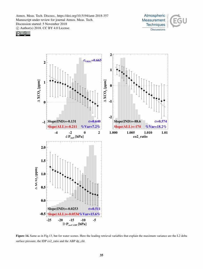
-4 -2 0 2d Psurf [hPa]

-1

0

1

2

∆ X

CO

2 [

pp

m]

-1

0

1

2σORIG=0.665

σ=0.640

%Var=7.2%

Slope(IND)=-0.131

Slope(ALL)=-0.211

1.000 1.005 1.010 1.015co2_ratio

-2

-1

0

1

2

∆ X

CO

2 [

pp

m]

-2

-1

0

1

2

σ=0.574

%Var=18.2%

Slope(IND)=-88.6

Slope(ALL)=-174

-25 -20 -15 -10 -5D Psurf,ABP [hPa]

-0.5

0.0

0.5

1.0

1.5

2.0

∆ X

CO

2 [

pp

m]

-0.5

0.0

0.5

1.0

1.5

2.0

σ=0.511

%Var=15.6%

Slope(IND)=-0.0253

Slope(ALL)=-0.0534

Figure 14. Same as in Fig.13, but for water scenes. Here the leading retrieval variables that explain the maximum variance are the L2 delta

surface pressure, the IDP co2_ratio and the ABP dp_cld.

35


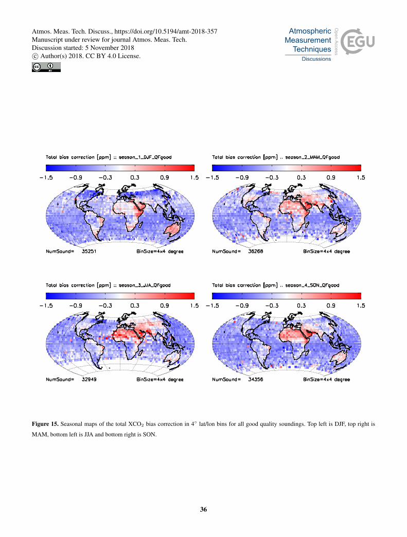
Figure 15. Seasonal maps of the total XCO2 bias correction in 4◦ lat/lon bins for all good quality soundings. Top left is DJF, top right is

MAM, bottom left is JJA and bottom right is SON.

36


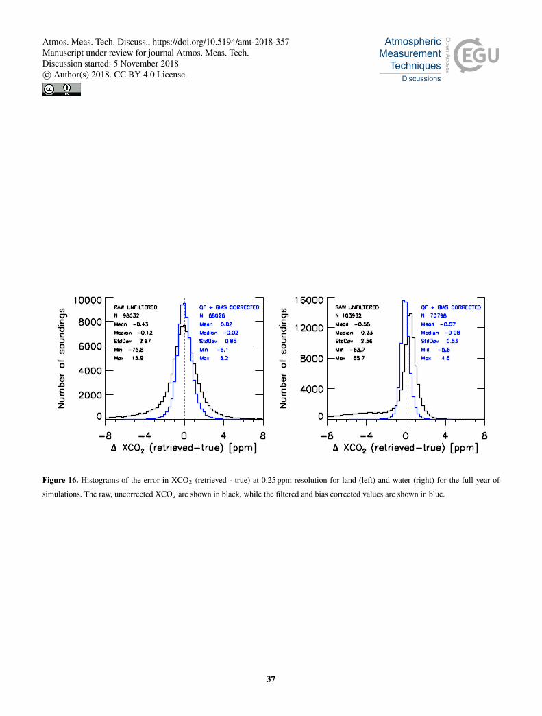
Figure 16. Histograms of the error in XCO2 (retrieved - true) at 0.25 ppm resolution for land (left) and water (right) for the full year of

simulations. The raw, uncorrected XCO2 are shown in black, while the filtered and bias corrected values are shown in blue.

37


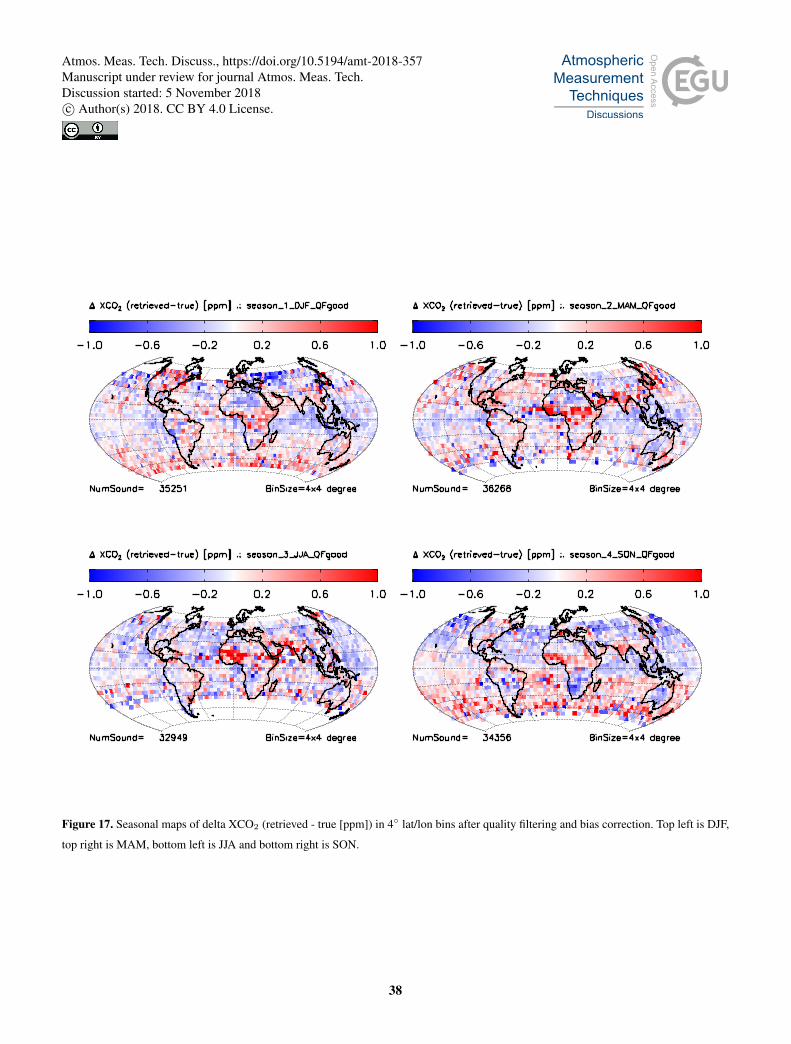
Figure 17. Seasonal maps of delta XCO2 (retrieved - true [ppm]) in 4◦ lat/lon bins after quality filtering and bias correction. Top left is DJF,

top right is MAM, bottom left is JJA and bottom right is SON.

38


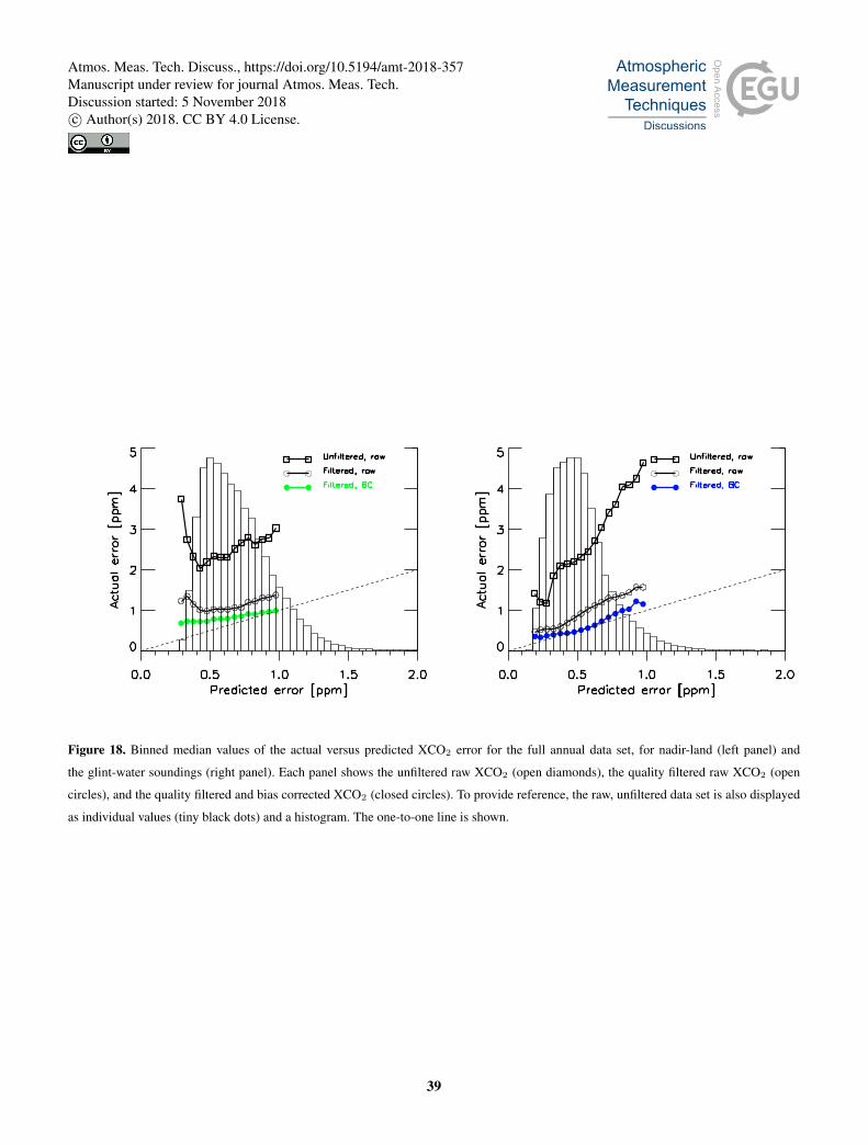
Figure 18. Binned median values of the actual versus predicted XCO2 error for the full annual data set, for nadir-land (left panel) and

the glint-water soundings (right panel). Each panel shows the unfiltered raw XCO2 (open diamonds), the quality filtered raw XCO2 (open

circles), and the quality filtered and bias corrected XCO2 (closed circles). To provide reference, the raw, unfiltered data set is also displayed

as individual values (tiny black dots) and a histogram. The one-to-one line is shown.

39


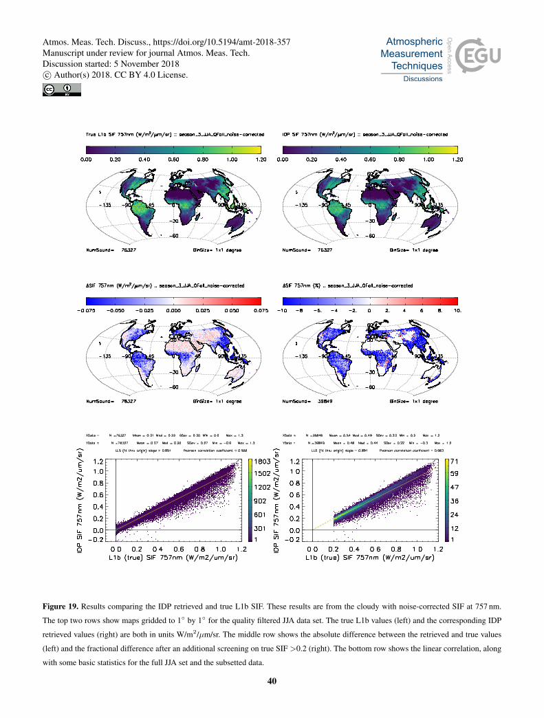
Figure 19. Results comparing the IDP retrieved and true L1b SIF. These results are from the cloudy with noise-corrected SIF at 757 nm.

The top two rows show maps gridded to 1◦ by 1◦ for the quality filtered JJA data set. The true L1b values (left) and the corresponding IDP

retrieved values (right) are both in units W/m2/µm/sr. The middle row shows the absolute difference between the retrieved and true values

(left) and the fractional difference after an additional screening on true SIF >0.2 (right). The bottom row shows the linear correlation, along

with some basic statistics for the full JJA set and the subsetted data.

40


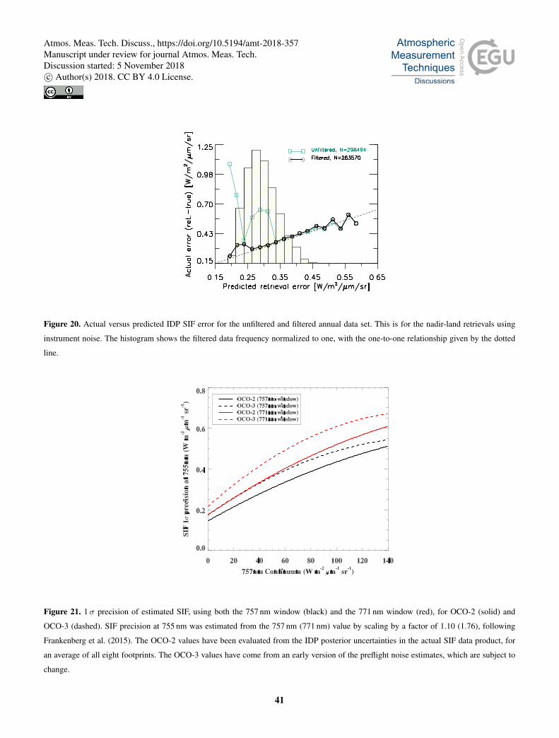
Figure 20. Actual versus predicted IDP SIF error for the unfiltered and filtered annual data set. This is for the nadir-land retrievals using

instrument noise. The histogram shows the filtered data frequency normalized to one, with the one-to-one relationship given by the dotted

line.

Figure 21. 1σ precision of estimated SIF, using both the 757 nm window (black) and the 771 nm window (red), for OCO-2 (solid) and

OCO-3 (dashed). SIF precision at 755 nm was estimated from the 757 nm (771 nm) value by scaling by a factor of 1.10 (1.76), following

Frankenberg et al. (2015). The OCO-2 values have been evaluated from the IDP posterior uncertainties in the actual SIF data product, for

an average of all eight footprints. The OCO-3 values have come from an early version of the preflight noise estimates, which are subject to

change.

41


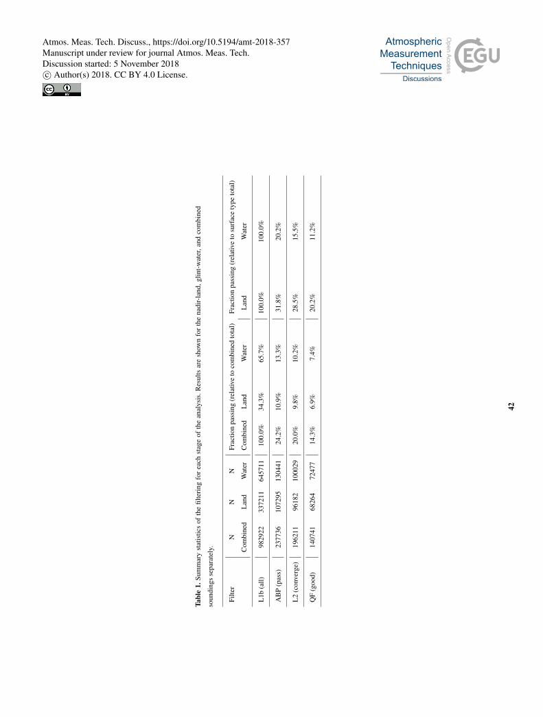
Tabl

e1.

Sum

mar

yst

atis

tics

ofth

efil

teri

ngfo

rea

chst

age

ofth

ean

alys

is.R

esul

tsar

esh

own

for

the

nadi

r-la

nd,g

lint-

wat

er,a

ndco

mbi

ned

soun

ding

sse

para

tely

.

Filte

rN

NN

Frac

tion

pass

ing

(rel

ativ

eto

com

bine

dto

tal)

Frac

tion

pass

ing

(rel

ativ

eto

surf

ace

type

tota

l)

Com

bine

dL

and

Wat

erC

ombi

ned

Lan

dW

ater

Lan

dW

ater

L1b

(all)

9829

2233

7211

6457

1110

0.0%

34.3

%65

.7%

100.

0%10

0.0%

AB

P(p

ass)

2377

3610

7295

1304

4124

.2%

10.9

%13

.3%

31.8

%20

.2%

L2

(con

verg

e)19

6211

9618

210

0029

20.0

%9.

8%10

.2%

28.5

%15

.5%

QF

(goo

d)14

0741

6826

472

477

14.3

%6.

9%7.

4%20

.2%

11.2

%

42


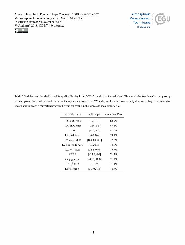
Table 2. Variables and thresholds used for quality filtering in the OCO-3 simulations for nadir-land. The cumulative fraction of scenes passing

are also given. Note that the need for the water vapor scale factor (L2 WV scale) is likely due to a recently discovered bug in the simulator

code that introduced a mismatch between the vertical profile in the scene and meteorology files.

Variable Name QF range Cum Frac Pass

IDP CO2 ratio [0.9, 1.03] 88.7%

IDP H2O ratio [0.88, 1.1] 85.6%

L2 dp [-6.0, 7.0] 81.6%

L2 total AOD [0.0, 0.4] 79.1%

L2 water AOD [0.0008, 0.1] 77.3%

L2 fine mode AOD [0.0, 0.08] 74.8%

L2 WV scale [0.84, 0.95] 73.7%

ABP dp [-25.0, 4.0] 71.7%

CO2 grad del [-40.0, 40.0] 71.2%

L2 χ2 O2A [0, 1.25] 71.1%

L1b signal 31 [0.075, 0.4] 70.7%

43


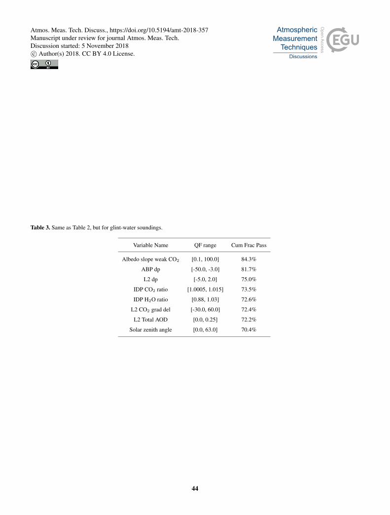
Table 3. Same as Table 2, but for glint-water soundings.

Variable Name QF range Cum Frac Pass

Albedo slope weak CO2 [0.1, 100.0] 84.3%

ABP dp [-50.0, -3.0] 81.7%

L2 dp [-5.0, 2.0] 75.0%

IDP CO2 ratio [1.0005, 1.015] 73.5%

IDP H2O ratio [0.88, 1.03] 72.6%

L2 CO2 grad del [-30.0, 60.0] 72.4%

L2 Total AOD [0.0, 0.25] 72.2%

Solar zenith angle [0.0, 63.0] 70.4%

44


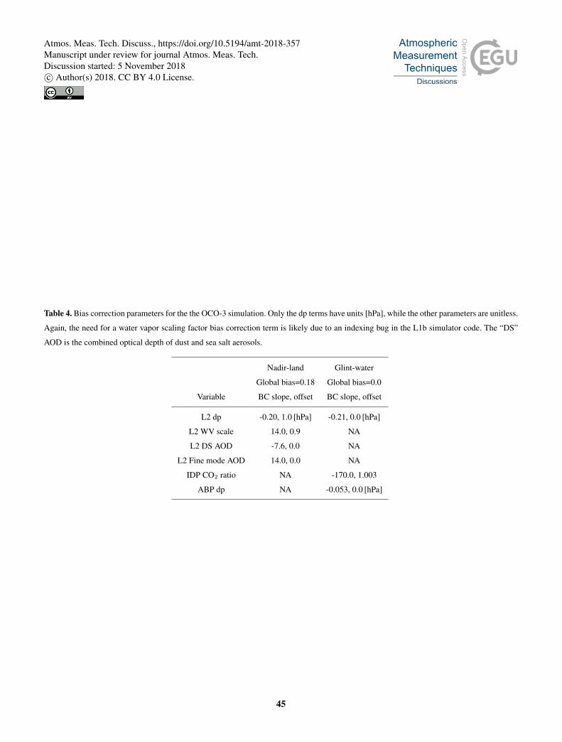
Table 4. Bias correction parameters for the the OCO-3 simulation. Only the dp terms have units [hPa], while the other parameters are unitless.

Again, the need for a water vapor scaling factor bias correction term is likely due to an indexing bug in the L1b simulator code. The “DS”

AOD is the combined optical depth of dust and sea salt aerosols.

Nadir-land Glint-water

Global bias=0.18 Global bias=0.0

Variable BC slope, offset BC slope, offset

L2 dp -0.20, 1.0 [hPa] -0.21, 0.0 [hPa]

L2 WV scale 14.0, 0.9 NA

L2 DS AOD -7.6, 0.0 NA

L2 Fine mode AOD 14.0, 0.0 NA

IDP CO2 ratio NA -170.0, 1.003

ABP dp NA -0.053, 0.0 [hPa]

45


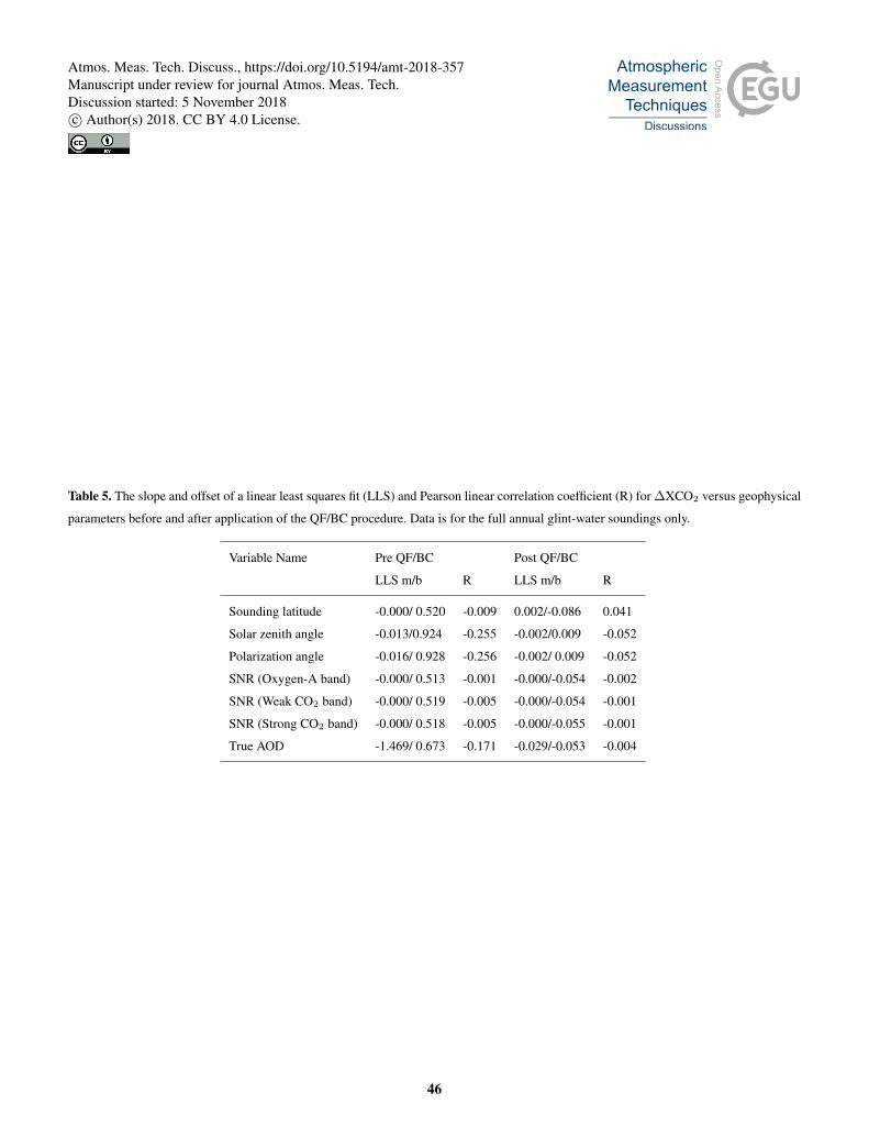
Table 5. The slope and offset of a linear least squares fit (LLS) and Pearson linear correlation coefficient (R) for ∆XCO2 versus geophysical

parameters before and after application of the QF/BC procedure. Data is for the full annual glint-water soundings only.

Variable Name Pre QF/BC Post QF/BC

LLS m/b R LLS m/b R

Sounding latitude -0.000/ 0.520 -0.009 0.002/-0.086 0.041

Solar zenith angle -0.013/0.924 -0.255 -0.002/0.009 -0.052

Polarization angle -0.016/ 0.928 -0.256 -0.002/ 0.009 -0.052

SNR (Oxygen-A band) -0.000/ 0.513 -0.001 -0.000/-0.054 -0.002

SNR (Weak CO2 band) -0.000/ 0.519 -0.005 -0.000/-0.054 -0.001

SNR (Strong CO2 band) -0.000/ 0.518 -0.005 -0.000/-0.055 -0.001

True AOD -1.469/ 0.673 -0.171 -0.029/-0.053 -0.004

46


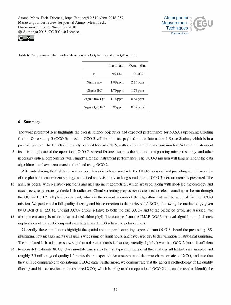
Table 6. Comparison of the standard deviation in XCO2 before and after QF and BC.

Land-nadir Ocean-glint

N 96,182 100,029

Sigma raw 1.88 ppm 2.15 ppm

Sigma BC 1.79 ppm 1.76 ppm

Sigma raw QF 1.14 ppm 0.67 ppm

Sigma QF, BC 0.85 ppm 0.52 ppm

6 Summary

The work presented here highlights the overall science objectives and expected performance for NASA’s upcoming Orbiting

Carbon Observatory-3 (OCO-3) mission. OCO-3 will be a hosted payload on the International Space Station, which is in a

precessing orbit. The launch is currently planned for early 2019, with a nominal three year mission life. While the instrument

itself is a duplicate of the operational OCO-2, several features, such as the addition of a pointing mirror assembly, and other5

necessary optical components, will slightly alter the instrument performance. The OCO-3 mission will largely inherit the data

algorithms that have been tested and refined using OCO-2.

After introducing the high level science objectives (which are similar to the OCO-2 mission) and providing a brief overview

of the planned measurement strategy, a detailed analysis of a year long simulation of OCO-3 measurements is presented. The

analysis begins with realistic ephemeris and measurement geometries, which are used, along with modeled meteorology and10

trace gases, to generate synthetic L1b radiances. Cloud screening preprocessors are used to select soundings to be run through

the OCO-2 B8 L2 full physics retrieval, which is the current version of the algorithm that will be adopted for the OCO-3

mission. We performed a full quality filtering and bias correction to the retrieved L2 XCO2, following the methodology given

by O’Dell et al. (2018). Overall XCO2 errors, relative to both the true XCO2 and to the predicted error, are assessed. We

also present analysis of the solar induced chlorophyll fluorescence from the IMAP DOAS retrieval algorithm, and discuss15

implications of the spatiotemporal sampling from the ISS relative to polar orbiters.

Generally, these simulations highlight the spatial and temporal sampling expected from OCO-3 aboard the precessing ISS,

illustrating how measurements will span a wide range of sunlit hours, and have large day to day variation in latitudinal sampling.

The simulated L1b radiances show signal to noise characteristic that are generally slightly lower than OCO-2, but still sufficient

to accurately estimate XCO2. Over monthly timescales that are typical of the global flux analysis, all latitudes are sampled and20

roughly 2.5 million good quality L2 retrievals are expected. An assessment of the error characteristics of XCO2 indicate that

they will be comparable to operational OCO-2 data. Furthermore, we demonstrate that the general methodology of L2 quality

filtering and bias correction on the retrieved XCO2 which is being used on operational OCO-2 data can be used to identify the

47


most useful data and reduce the bias inherent in the full physics retrieval algorithm. In fact, the filtering and bias correction

process is necessary in order to meet the measurement objectives.

Retrievals of SIF using the IDP algorithm are also expected to have similar error characteristics compared to OCO-2, espe-

cially with respect to error induced by instrument noise. This new set of space-based SIF will be highly informative because

of the varying time of day sampling, so important to characterizing the local behavior of SIF. The dense coverage of latitudes5

below about 50◦, where global SIF is most active on an annual scale, is expected to provide a rich data set to the science

community.

Overall, the OCO-3 performance characteristics, as assessed in this simulation, should provide a global dataset that achieves

the mission goals and continues the dense, high-precision XCO2 and SIF record from space-borne measurements.

48


Author contributions. The overall research goals were crafted by AE, with contributions from CWO and TET. RP provided the OCO-3

simulated geometry, with input from AE. TET generated the L1b radiances and ran the ABP and IDP preprocessors. AE ran the L2 FP

retrievals and CWO performed the quality filtering and bias correction procedure. The data analysis and word smithing were joint efforts

between TET, CWO and AE. The figures were generated by TET, with input from CWO and AE.

Competing interests. We declare no competing interests in this work.5

Acknowledgements. A portion of the research described in this paper was carried out at the Jet Propulsion Laboratory, California Institute of

Technology, under a contract with the National Aeronautics and Space Administration. The CSU contribution to this work was supported by

JPL subcontract 1439002.

We would like to acknowledge the hard work of the OCO-3 calibration team for providing data necessary to generate the L1b simulations.

49


References

Aben, I., Hasekamp, O., and Hartmann, W.: Uncertainties in the space-based measurements of CO2 columns due to scattering in the Earth’s

atmosphere, J. Quant. Spectrosc. Radiat. Transfer, 104, 450–459, 2007.

Basilio, R., Bennett, M., Boland, S., Crisp, D., Eldering, A., Ellis, A., Glavich, T., Gunson, M., Khaki, S., and Pollock, R.: SYSTEMS

DESIGN AND IMPLEMENTATION OF THE PROPOSED ORBITING CARBON OBSERVATORY-3 ON THE INTERNATIONAL5

SPACE STATION’S JAPANESE EXPERIMENTAL MODULE, Science and Technology Series, 114, 321–323, 2013.

Basu, S., Krol, M., Butz, A., Clerbaux, C., Sawa, Y., Machida, T., Matsueda, H., Frankenberg, C., Hasekamp, O., and Aben, I.: The seasonal

variation of the CO2 flux over Tropical Asia estimated from GOSAT, CONTRAIL, and IASI, Geophysical Research Letters, 41, 1809–

1815, 2014.

Beer, C., Reichstein, M., Tomelleri, E., Ciais, P., Jung, M., Carvalhais, N., Rodenbeck, C., Arain, M. A., Baldocchi, D., Bonan, G. B.,10

Bondeau, A., Cescatti, A., Lasslop, G., Lindroth, A., Lomas, M., Luyssaert, S., Margolis, H., Oleson, K. W., Roupsard, O., Veenendaal,

E., Viovy, N., Williams, C., Woodward, F. I., and Papale, D.: Terrestial gross carbon dioxide uptake: Global distribution and covariation

with climate, Science, https://doi.org/10.1116/science.1184984, 2010.

Boesch, H., Brown, L., Castano, R., Christi, M., Connor, B., Crisp, D., Eldering, A., Fisher, B., Frankenberg, C., Gunson, M., Granat,

R., McDuffie, J., Miller, C., Natraj, V., O’Brien, D., O’Dell, C., Osterman, G., Oyafuso, F., Payne, V., Polonsky, I., Smyth, M., Spurr,15

R., Thompson, D., and Toon, G.: Orbiting Carbon Observatory (OCO)-2 Level 2 Full Physics, Algorithm Theoretical Basis Document

D-55207, Jet Propulsion Laboratory, 2015.

Bösch, H., Toon, G. C., Sen, B., Washenfelder, R. A., Wennberg, P. O., Buchwitz, M., de Beek, R., Burrows, J. P., Crisp, D., Christi,

M., Connor, B. J., Natraj, V., and Yung, Y. L.: Space-based near-infrared CO2 measurements: Testing the Orbiting Carbon Observatory

retrieval algorithm and validation concept using SCIAMACHY observations over Park Falls, Wisconsin, J. Geophys. Res., 111, D23302,20

https://doi.org/10.1029/2006JD007080, 2006.

Buchwitz, M., Reuter, M., Schneising, O., Boesch, H., Guerlet, S., Dils, B., Aben, I., Armante, R., Bergamaschi, P., and Blumenstock, T.:

The Greenhouse Gas Climate Change Initiative (GHG-CCI): Comparison and quality assessment of near-surface-sensitive satellite-derived

CO2 and CH4 global data sets, RSE, 162, 344–362, 2015.

Buil, C., Pascal, V., Loesel, J., Pierangelo, C., Roucayrol, L., and Tauziede, L.: A new space instrumental concept for the measurement of25

CO2 concentration in the atmosphere, in: SPIE Remote Sensing, pp. 817 621–817 621–11, International Society for Optics and Photonics,

2011.

Butz, A., Hasekamp, O., Frankenberg, C., and Aben, I.: Retrievals of atmospheric CO2 from simulated space-borne measurements of

backscattered near-infrared sunlight: accounting for aerosol effects, Appl. Opt., 48, 3322–3336, https://doi.org/10.1364/AO.48.003322,

2009.30

Chatterjee, A., Gierach, M., Sutton, A., Feely, R., Crisp, D., Eldering, A., Gunson, M., O’dell, C., Stephens, B., and Schimel, D.: Influence

of El Niño on atmospheric CO2 over the tropical Pacific Ocean: Findings from NASA’s OCO-2 mission, Science, 358, eaam5776, 2017.

Connor, B. J., Boesch, H., Toon, G., Sen, B., Miller, C., and Crisp, D.: Orbiting Carbon Observatory: Inverse method and prospective error

analysis, J. Geophys. Res., 113, D05 305, https://doi.org/10.1029/2006JD008336, 2008.

Crisp, D., Pollock, H. R., Rosenberg, R., Chapsky, L., Lee, R. A., Oyafuso, F. A., Frankenberg, C., O’Dell, C. W., Brueffe, C. J., Doran, G. B.,35

Eldering, A., Fisher, B. M., Fu, D., Gunson, M. R., Mandrake, L., Osterman, G. B., Schwandner, F. M., Sun, K., Taylor, T. E., , Wennberg,

50


P. O., and Wunch, D.: The on-orbit performance of the Orbiting Carbon Observatory-2 (OCO-2) instrument and its radiometrically

calibrated products, Atmos. Meas. Tech., 10, 59–81, https://doi.org/10.5194/amt-10-59-2017, 2017.

Detmers, R., Hasekamp, O., Aben, I., Houweling, S., Leeuwen, T., Butz, A., Landgraf, J., Köhler, P., Guanter, L., and Poulter, B.: Anomalous

carbon uptake in Australia as seen by GOSAT, Geophysical Research Letters, 42, 8177–8184, 2015.

Dubayah, R., Goetz, S., Blair, J. B., Fatoyinbo, T., Hansen, M., Healey, S., Hofton, M., Hurtt, G., Kellner, J., and Luthcke, S.: The global5

ecosystem dynamics investigation, in: AGU Fall Meeting Abstracts, 2014.

Eldering, A., O’Dell, C. W., Wennberg, P. O., Crisp, D., Gunson, M. R., Viatte, C., Avis, C., Braverman, A., Castano, R., Chang, A.,

Chapsky, L., Cheng, C., Connor, B., Dang, L., Doran, G., Fisher, B., Frankenberg, C., Fu, D., Granat, R., Hobbs, J., Lee, R. A., Mandrake,

L., McDuffie, J., Miller, C. E., Myers, V., Natraj, V., O’Brien, D., Osterman, G. B., Oyafuso, F., ayne, V. H., Pollock, H. R., Polonsky,

I., Roehl, C. M., Rosenberg, R., Schwandner, F., Smyth, M., Tang, V., Taylor, T. E., To, C., Wunch, D., and Yoshimizu, J.: The Orbiting10

Carbon Observatory-2: first 18 months of science data products, Atmos. Meas. Tech., 10, 549–563, https://doi.org/10.5194/amt-10-549-

2017, 2017a.

Eldering, A., Wennberg, P., Crisp, D., Schimel, D., Gunson, M., Chatterjee, A., Liu, J., Schwandner, F., Sun, Y., and O’Dell, C.: The Orbiting

Carbon Observatory-2 early science investigations of regional carbon dioxide fluxes, Science, 358, eaam5745, 2017b.

Fisher, J., Hook, S., Allen, R., Anderson, M., French, A., Hain, C., Hulley, G., and Wood, E.: ECOSTRESS: NASA’s next-generation mission15

to measure evapotranspiration from the International Space Station, in: AGU Fall Meeting Abstracts, 2015.

Frankenberg, C., Butz, A., and Toon, G.: Disentangling chlophyll fluorescence from atmospheric scatting effects in the O2 A band spectra of

reflected sunlight, Geophysical Research Letters, 38, 2011.

Frankenberg, C., O’Dell, C., Guanter, L., and McDuffie, J.: Remote sensing of near-infrared chlorophyll fluorescence from space in scattering

atmospheres: implications for its retrieval and interferences with atmospheric CO2 retrievals, Atmospheric Measurement Techniques, 5,20

2081–2094, 2012.

Frankenberg, C., O’Dell, C., Berry, J., Guanter, L., Joiner, J., Kohler, P., Pollock, R., and Taylor, T. E.: Prospects for chlorophyll fluorescence

remote sensing from the Orbiting Carbon Observatory-2, RSE, 147, 1–12, https://doi.org/10.1016/j.rse/2014.02.007, 2014.

Guerlet, S., Basu, S., Butz, A., Krol, M., Hahne, P., Houweling, S., Hasekamp, O., and Aben, I.: Reduced carbon uptake during the 2010

Northern Hemisphere summer from GOSAT, Geophysical Research Letters, 40, 2378–2383, 2013.25

Hulley, G., Hook, S., Fisher, J., and Lee, C.: ECOSTRESS, a NASA Eart-Ventures instrument for studying links between the wa-

ter cycle and plant health over the diurnal cycle, in: IEEE International Geoscience and Remote Sensing Symposium (IGARSS),

https://doi.org/10.1109/IGARSS.2017.8128248, 2017.

Kuze, A., Suto, H., Nakajima, M., and Hamazaki, T.: Thermal and near infrared sensor for carbon observation Fourier-transform spectrometer

on the Greenhouse Gases Observing Satellite for greenhouse gases monitoring, Appl. Opt., 48, 6716–6733, 2009.30

Lindqvist, H., O’Dell, C., Basu, S., Bösch, H., Chevallier, F., Deutscher, N., Feng, L., Fisher, B., Hase, F., and Inoue, M.: Does GOSAT

capture the true seasonal cycle of carbon dioxide?, Atmos. Chem. Phys, 15, 13 023–13 040, 2015.

Liu, J., K., B., Lee, M., Henze, D., Bousserez, N., Brix, H., Collatz, G., Menemenlis, D., Ott, L., Pawson, S., Jones, D., and Nassar,

R.: Carbon monitoring system flux estimation and attribution: impact of ACOS-GOSAT XCO2 sampling on the inference of terrestrial

biospheric sources and sinks, Tellus B, 66, https://doi.org/10.3402/tellusb.v66.22486, 2014.35

Liu, J., Bowman, K. W., Schimel, D. S., Parazoo, N. C., Jiang, Z., Lee, M., Bloom, A. A., Wunch, D., Frankenberg, C., and Sun, Y.:

Contrasting carbon cycle responses of the tropical continents to the 2015–2016 El Niño, Science, 358, eaam5690, 2017.

51


Matsunaga, T., Iwasaki, A., Tsuchida, S., Tanii, J., Kashimura, O., Nakamura, R., Yamamoto, H., Tachikawa, T., and Rokugawa, S.: Hyper-

spectral Imager Suite (HISUI), Optical Payloads for Space Missions, pp. 215–222, 2015.

Matsunaga, T., Iwasaki, A., Tsuchida, S., Tanii, J., Kashimura, O., Nakamura, R., Yamamoto, H., Tachikawa, T., and Rokugawa, S.: Current

status of Hyperspectral Imager Suite (HISUI) onboard International Space Station (ISS), in: IEEE International Geoscience and Remote

Sensing Symposium (IGARSS), https://doi.org/10.1109/IGARSS.2017.8126989, 2017.5

Miller, C., Crisp, D., DeCola, P., Olsen, S., Randerson, J., Michalak, A., Alkhaled, A., Rayner, P., Jacob, D., Suntharalingam, P., Jones, D.,

Denning, A., Nicholls, M., Doney, S., Pawson, S., Boesch, H., Connor, B., Fung, I., O’Brien, D., Salawitch, R., Sander, S., Sen, B., Tans,

P., Toon, G., Wennberg, P., Wofsy, S., Yung, Y., and Law, R.: Precision requirements for space-based XCO2 data, J. Geophys. Res., 112,

https://doi.org/10.1029/2006JD007659, 2007.

Mishchenko, M. I., Cairns, B., Kopp, G., Schueler, C. F., Fafaul, B. A., Hansen, J. E., Hooker, R. J., Itchkawich, T., Maring, H. B., and Travis,10

L. D.: Accurate monitoring of terrestrial aerosols and total solar irradiance: introducing the Glory Mission, Bulletin of the American

Meteorological Society, 88, 677–692, 2007.

Nakajima, M., Kuze, A., and Suto, H.: The current status of GOSAT and the concept of GOSAT-2, in: SPIE 8533, Sensors, Systems, and Next-

Generation Satellites XVI, pp. 853 306–853 306–10, International Society for Optics and Photonics, http://dx.doi.org/10.1117/12.974954,

2012.15

Nelson, R., O’Dell, C. W., Taylor, T. E., Mandrake, L., and Smyth, M.: The potential of clear-sky carbon dioxide satellite retrievals, Atmos.

Meas. Tech., 9, 1671–1684, https://doi.org/10.5194/amt-9-1671-2016, 2016.

O’Brien, D. M., Polonsky, I., O’Dell, C., and Carheden, A.: Orbiting Carbon Observatory (OCO), Algorithm Theoretical Basis Document:

The OCO simulator, Technical Report ISSN 0737-5352-85, Cooperative Institute for Research in the Atmosphere, Colorado State Univer-

sity, ftp://ftp.cira.colostate.edu/ftp/TTaylor/publications/20090813_OCO_simulator.pdf, 2009.20

O’Brien, D. M., Polonsky, I., Utembe, S. R., and Rayner, P. J.: Potential of a geostationary geoCARB mission to estimate surface emissions of

CO2, CH4 and CO in a polluted urban environment: case study Shanghai, Atmos. Meas. Tech., 9, 4633–4654, https://doi.org/10.5194/amt-

9-4633-2016, 2016.

Oda, T. and Maksyutov, S.: A very high-resolution (1 km x 1 km) global fossil fuel CO2 emission inventory derived using a point source

database and satellite observations of nighttime lights, Atmos. Chem. Phys., 11, 543–556, https://doi.org/10.5194/acp-11-543-2011, https:25

//www.atmos-chem-phys.net/11/543/2011/, 2011.

Oda, T., Maksyutov, S., and Andres, R. J.: The Open-source Data Inventory for Anthropogenic CO2, version 2016 (ODIAC2016): a global

monthly fossil fuel CO2 gridded emissions data product for tracer transport simulations and surface flux inversions, Earth System Science

Data, 10, 87–107, https://doi.org/10.5194/essd-10-87-2018, https://www.earth-syst-sci-data.net/10/87/2018/, 2018.

O’Dell, C. W., Connor, B., Bösch, H., O’Brien, D., Frankenberg, C., Castano, R., Christi, M., Crisp, D., Eldering, A., Fisher, B., Gunson,30

M., McDuffie, J., Miller, C. E., Natraj, V., Oyafuso, F., Polonsky, I., Smyth, M., Taylor, T., Toon, G. C., Wennberg, P. O., and Wunch,

D.: The ACOS CO2 retrieval algorithm–Part 1: Description and validation against synthetic observations, Atmos. Meas. Tech., 5, 99–121,

https://doi.org/10.5194/amt-5-99-2012, 2012.

O’Dell, C. W., Eldering, A., Wennberg, P. O., Crisp, D., Gunson, M. R., Fisher, B., Frankenberg, C., Kiel, M., Lindqvist, H., Mandrake,

L., Merrelli, A., Natraj, V., Nelson, R. R., Osterman, G. B., Payne, V. H., Taylor, T. R., Wunch, D., Drouin, B. J., Oyafuso, F., Chang,35

A., McDuffie, J., Smyth, M., Baker, D. F., Basu, S., Chevallier, F., Crowell, S. M. R., Feng, L., Palmer, P. I., Dubey, M., García, O. E.,

Griffith, D. W. T., Hase, F., Iraci, L. T., Kivi, R., Morino, I., Notholt, J., Ohyama, H., Petri, C., Roehl, C. M., Sha, M. K., Strong, K.,

Sussmann, R., Te, Y., Uchino, O., and Velazco, V. A.: Improved Retrievals of Carbon Dioxide from the Orbiting Carbon Observatory-2

52


with the version 8 ACOS algorithm, Atmospheric Measurement Techniques Discussions, 2018, 1–57, https://doi.org/10.5194/amt-2018-

257, https://www.atmos-meas-tech-discuss.net/amt-2018-257/, 2018.

Parazoo, N. C., Bowman, K., Fisher, J. B., Frankenberg, C., Jones, D., Cescatti, A., Perez-Priego, O., Wohlfahrt, G., and Montagnani, L.:

Terrestrial gross primary production inferred from satellite fluorescence and vegetation models, Global change biology, 20, 3103–3121,

2014.5

Persh, S., Shaham, Y., Benami, O., Cairns, B., Mishchenko, M. I., Hein, J. D., and Fafaul, B. A.: Ground performance measurements of the

Glory aerosol polarimetry sensor, in: Earth Observing Systems XV, vol. 7807, p. 780703, International Society for Optics and Photonics,

2010.

Peters, W., Jacobson, A. R., Sweeney, C., Andrews, A. E., Conway, T. J., Masarie, K., Miller, J. B., Bruhwiler, L. M., Pétron, G., and Hirsch,

A. I.: An atmospheric perspective on North American carbon dioxide exchange: CarbonTracker, Proceedings of the National Academy of10

Sciences, 104, 18 925–18 930, 2007.

Reuter, M., Bösch, H., Bovensmann, H., Bril, A., Buchwitz, M., Butz, A., Burrows, J., O’Dell, C., Guerlet, S., and Hasekamp, O.: A joint

effort to deliver satellite retrieved atmospheric CO2 concentrations for surface flux inversions: the ensemble median algorithm EMMA,

Atmospheric Chemistry and Physics, 13, 1771–1780, 2013.

Rosenberg, R., Maxwell, S., Johnson, B. C., Chapsky, L., Lee, R., and Pollock, R.: Preflight radiometric calibration of the Orbiting Carbon15

Observatory 2, TGRS, 55, 1994–2006, https://doi.org/10.1109/TGRS.2016.2634023, 2017.

Ross, A. N., Wooster, M. J., Bösch, H., and Parker, R.: First satellite measurements of carbon dioxide and methane emission ratios in wildfire

plumes, Geophysical Research Letters, 40, 4098–4102, 2013.

Saha, S., Moorthi, S., Wu, X., Wang, J., Nadiga, S., Tripp, P., Behringer, D., Hou, Y.-T., ya Chuang, H., Iredell, M., Ek, M., Meng, J., Yang,

R., Mendez, M. P., van den Dool, H., Zhang, Q., Wang, W., Chen, M., and Becker, E.: The NCEP Climate Forecast System Version 2, J.20

Climate., 27, 2185–2208, https://doi.org/10.1175/JCL-D-12-00823.1, 2014.

Schaaf, C. B., Gao, F., Strahler, A. H., Lucht, W., Li, X., Tsang, T., Strugnell, N. C., Zhang, X., Jin, Y., Muller, J.-P., Lewis, P., Barnsley,

M., Hobson, P., Disney, M., Roberts, G., Dunderdale, M., Doll, C., d’Entremont, R. P., Hu, B., Liang, S., Privette, J. L., and Roy, D.: First

operational BRDF, albedo nadir reflectance products from MODIS, Remote Sens. Environ., 83, 135–148, https://doi.org/10.1016/S00034-

4257(02)00091-3, 2002.25

Schwandner, F. M., Gunson, M. R., Miller, C. E., Carn, S. A., Eldering, A., Krings, T., Verhulst, K. R., Schimel, D. S., Nguyen, H. M., and

Crisp, D.: Spaceborne detection of localized carbon dioxide sources, Science, 358, eaam5782, 2017.

Stavros, E. N., Schimel, D., Pavlick, R., Serbin, S., Swann, A., Duncanson, L., Fisher, J. B., Fassnacht, F., Ustin, S., and Dubayah, R.: ISS

observations offer insights into plant function, Nature Ecology & Evolution, 1, s41 559–017–0194, 2017.

Stysley, P. R., Coyle, D. B., Kay, R. B., Frederickson, R., Poulious, D., Cory, K., and Clarke, G.: Long term performance of the High Output30

Maximum Efficiency Resonator (HOMER) laser for NASA’s Global Ecosystem Dynamics Investigation (GEDI) lidar, Optics & Laser

Technology, 68, 67–72, https://doi.org/10.1016/j.optlastec.2014.11.001, 2015.

Sun, Y., Frankenberg, C., Wood, J. D., Schimel, D. S., Jung, M., Guanter, L., Drewry, D., Verma, M., Porcar-Castell, A., Griffis, T. J., et al.:

OCO-2 advances photosynthesis observation from space via solar-induced chlorophyll fluorescence, Science, 358, eaam5747, 2017.

Sun, Y., Frankenberg, C., Jung, M., Joiner, J., Guanter, L., Kohler, P., and Magney, T.: Overview of the solar-induced chlorophyll fluorescence35

SIF from the Orbiting Carbon Observatory-2: Retrieval, cross-mission comparison, and global monitoring for GPP, RSE, 209, 808–823,

https://doi.org/10.1016/j.rse/2018.02.016, 2018.

53


Taylor, T. E., O’Dell, C. W., Frankenberg, C., Partain, P. T., Cronk, H. Q., Savtchenko, A., Nelson, R. R., Rosenthal, E. J., Chang, A., Fisher,

B. M., Osterman, G. B., Pollock, R. H., Crisp, D., Eldering, A., and Gunson, M. R.: Orbiting Carbon Observatory-2 (OCO-2) cloud screen-

ing algorithms: validation against collocated MODIS and CALIOP data, Atmos. Meas. Tech., 9, 973–989, https://doi.org/10.5194/amt-9-

973-2016, 2016.

Thuillier, G., Hersé, M., Foujols, T., Peetermans, W., Gillotay, D., Simon, P., and Mandel, H.: The solar spectral irradiance from 200 to 24005

nm as measured by the SOLSPEC spectrometer from the ATLAS and EURECA missions, Solar Physics, 214, 1–22, 2003.

Toon, G., Blavier, J., Sen, B., Salawitch, R., Osterman, G., Notholt, J., Rex, M., McElroy, C., and Russell, J.: Groundbased observations of

Arctic O3 loss during spring and summer 1997, Journal of Geophysical Research: Atmospheres, 104, 26 497–26 510, 1999.

Wunch, D., Toon, G., Wennberg, P., Wofsy, S., Stephens, B., Fischer, M., Uchino, O., Abshire, J., Bernath, P., Biraud, S., Blavier, J., Boone,

C., Bowman, K., Browell, E., Campos, T., Connor, B., Daube, B., Deutsher, N., Diao, M., Elkins, J., Gerbig, C., Gottlieb, W., Griffith, D.,10

Hurst, D., Jimenez, R., Keppel-Aleks, G., Kort, E., Macatangay, R., Machida, T., Matsueda, H., Moore, F., Morino, I., Park, S., Robinson,

J., Roehl, C., Sawa, Y., Sherlock, V., Sweeney, C., Tanaka, T., and Zondlo, M.: Calibration of the Total Carbon Column Observing Network

using aircraft profile data, Atmos. Meas. Tech., 3, 1351–1362, https://doi.org/10.5194/amt-3-1351-2010, 2010.

Wunch, D., Wennberg, P., Toon, G., Connor, B., Fisher, B., Osterman, G., Frankenberg, C., Mandrake, L., O’Dell, C., P.Ahonen, Biraud,

S., Castano, R., Cressie, N., Crisp, D., Deutsher, N., Eldering, A., Fisher, M., Griffith, D., Heikkinen, M. G. P., Kyro, G. K.-A. E., Lin-15

denmaier, R., Macatangay, R., Mendonca, J., Messerschmidt, J., Miller, C., Morino, I., Notholt, J., Oyafuso, F., Rettinger, M., Robinson,

J., Roehl, C., Salawitch, R., Sherlock, V., Strong, K., Sussmann, R., Tanaka, T., Thompson, D., Uchino, O., Warneke, T., and Wofsy,

S.: A method for evaluating bias in global measurements of CO2 total columns from space, Atmos. Chem. Phys., 11, 12 317–12 337,

https://doi.org/10.5194/acp-11-12317-2011, 2011.

Wunch, D., Wennberg, P., Messerschmidt, J., Parazoo, N., Toon, G., Deutscher, N., Keppel-Aleks, G., Roehl, C., Randerson, J., and Warneke,20

T.: The covariation of Northern Hemisphere summertime CO2 with surface temperature in boreal regions, Atmospheric Chemistry and

Physics, 13, 9447–9459, 2013.

Wunch, D., Wennberg, P. O., Osterman, G., Fisher, B., Naylor, B., Roehl, C. M., O’Dell, C., Mandrake, L., Viatte, C., and Kiel, M.: Compar-

isons of the Orbiting Carbon Observatory-2 (OCO-2) X CO 2 measurements with TCCON, Atmospheric Measurement Techniques, 10,

2209, 2017.25

Yang, D., Liu, Y., Cai, Z., Chen, X., Yao, L., and Lu, D.: First Global Carbon Dioxide Maps Produced from TanSat Measurements, Adv.

Atmos. Sci., 35, https://doi.org/10.1007/s00376-018-7312-6, 2018.

54


The OCO-3 mission; measurement objectives and expected ...

Documents