The notion of observable in the covariant Hamiltonian formalism for the calculus of variations with several variables

arX

iv:m

ath-

ph/0

4010

47v1

27

Jan

2004

The notion of observable in the covariant Hamiltonian

formalism for the calculus of variations with several

variables

Frederic HELEIN∗

Institut de Mathmatiques de Jussieu, UMR 7586,

Universit Denis Diderot–Paris 7, Site de Chevaleret,16 rue Clisson 75013 Paris (France)

Joseph KOUNEIHER†

LUTH, CNRS UMR 8102Observatoire de Paris - section Meudon

5 Place Jules Janssen92195 Meudon Cedex

Universite Paris 7

February 7, 2008

Abstract

This papers is concerned with multisymplectic formalisms which are the frameworks forHamiltonian theories for fields theory. Our main purpose is to study the observable(n− 1)-forms which allows one to construct observable functionals on the set of solutionsof the Hamilton equations by integration. We develop here two different points of view:generalizing the law p, q = 1 or the law dF/dt = H,F. This leads to two possibledefinitions; we explore the relationships and the differences between these two concepts.We show that — in contrast with the de Donder–Weyl theory — the two definitionscoincides in the Lepage–Dedecker theory.

∗[email protected]†[email protected]

1 Introduction

Multisymplectic formalisms are the frameworks for finite dimensional formulations of vari-ational problems with several variables (or field theories for physicists) analogous to thewell-known Hamiltonian theory of point mechanics. They are based on the following ana-logues of symplectic forms: given a differential manifold M and n ∈ N a smooth (n+ 1)-form Ω on M is a multisymplectic form if and only if Ω is non degenerate (i.e.∀m ∈ M,∀ξ ∈ TmM, if ξ Ωm = 0, then ξ = 0) and closed. We call (M,Ω) a multisymplecticmanifold. Then one can associates to a Lagrangian variational problem a multisymplecticmanifold (M,Ω) and a Hamiltonian function H on M s.t. any solution of the variationalproblem is represented by a solution of a system of generalized Hamilton equations. Geo-metrically this solution is pictured by an n-dimensional submanifold Γ ⊂ M s.t.∀m ∈ Mthere exists a n-multivector X tangent to M at m s.t.X Ω = (−1)ndH. We then callΓ a Hamiltonian n-curve.

For example a variational problem on maps u : Rn −→ R can written as the system1

∂u

∂xµ=∂H

∂pµ(x, u, p) and

∑

µ

∂pµ

∂xµ= −

∂H

∂u(x, u, p). (1)

The corresponding multisymplectic form is Ω := dθ, where θ := eω + pµdu ∧ ωµ (andω := dx1 ∧ · · · ∧ dxn and ωµ := ∂µ ω). The simplest example of such a theory was pro-posed by T. de Donder [4] and H. Weyl [29]. But it is a particular case of a huge variety ofmultisymplectic theories which were discovered by T. Lepage and can be described usinga universal framework built by P. Dedecker [5], [13], [15].

The present paper, which is a continuation of [13] and [15], is devoted to the study of ob-servable functionals defined on the set of all Hamiltonian n-curves Γ. An important classof such functionals can be constructed by choosing appropriate (n − 1)-forms F on themultisymplectic manifold M and a hypersurface Σ of M which crosses transversally allHamiltonian n-curves (we shall call slices such hypersurfaces). Then

∫ΣF : Γ 7−→

∫Σ∩Γ

Fis such a functional. One should however check that such functionals measure physi-cally relevant quantities. The philosophy adopted here is inspired from quantum Physics:the formalism should provide us with rules for predicting the dynamical evolution of anobservable. There are two ways to translate this requirement mathematically: first the“infinitesimal evolution” dF (X) of F along a n-multivector X tangent to a Hamiltoniann-curve should be completely determined by the value of dH at the point — this leadsto the definition of what we call an observable (n − 1)-form (OF), the subject of Sec-tion 3; alternatively, inspired by an analogy with classical particle mechanics, one canassume that there exists a tangent vector field ξF such that ξF Ω + dF = 0 everywhere

1an obvious difference with mechanics is that there is a dissymmetry between the “position” variableu and the “momentum” variables pµ. Since (1) involves a divergence of pµ one can anticipate that, whenformulated in more geometrical terms, pµ will be interpreted as the components of a (n−1)-form, whereasu as a scalar function.

— we call such forms algebraic observable (n − 1)-forms (AOF). This point of view willbe investigated in Section 4. We believe that the notion of AOF was introduced by W.Tulczyjew in 1968 [27] (see also [8], [10], [22]). To our knowledge the notion of OF wasnever considered before; it seems to us however that it is a more natural definition. It iseasy to check that all AOF are actually OF but the converse is in general not true (seeSection 4), as in particular in the de Donder–Weyl theory.

It is worth here to insist on the difference of points of view between choosing OF’s orAOF’s. The definition of OF is in fact the right notion if we are motivated by the interplaybetween the dynamics and observable functionals. It allows us to define a pseudobracketH, F between the Hamiltonian function and an OF F which leads to a generalizationof the famous equation dA

dt= H,A of the Hamiltonian mechanics. This is the relation

dF|Γ = H, Fω|Γ, (2)

where Γ is a Hamiltonian n-curve and ω is a given volume n-form on space-time (seeProposition 3.1). In contrast the definition of AOF’s is the right notion if we are moti-vated in defining an analogue of the Poisson bracket between observable (n − 1)-forms.This Poisson bracket, for two AOL F and G is given by F,G := ξF ∧ξG Ω, a definitionreminiscent from classical mechanics. This allows us to construct a Poisson bracket onfunctionals by the rule

∫ΣF,∫ΣG : Γ 7−→

∫Σ∩Γ

F,G (see Section 4).

Note that it is possible to generalize the notion of observable (p−1)-forms to the case where0 ≤ p < n, as pointed out recently in [20], [21]. For example the dissymmetry betweenvariables u and pµ in system (1) suggests that, if the pµ’s are actually the components ofthe observable (n−1)-form pµωµ, u should be an observable function. Another interestingexample is the Maxwell action, where the gauge potential 1-form Aµdx

µ and the Faraday(n − 2)-form ⋆dA = ηµληνσ(∂µAν − ∂νAµ)ωλσ are also “observable”, as proposed in [20].Note that again two kinds of approaches for defining such observable forms are possible,as in the preceding paragraph: either our starting point is to ensure consistency withthe dynamics (this leads us in Section 3 to the definition of OF’s) or we privilege thedefinition which seems to be the more appropriate for having a notion of Poisson bracket(this leads us in Section 4 to the definition of AOF’s). If we were follow the second pointof view we would be led to the following definition, in [20]: a (p − 1)-form F would beobservable (“Hamiltonian” in [20]) if and only if there exists a (n − p + 1)-multivectorXF such that dF = (−1)n−p+1XF Ω. This definition has the advantage that — thanksto a consistent definition of Lie derivatives of forms with respect to multivectors due toW.M. Tulczyjew [28] — a beautiful notion of graded Poisson bracket between such formscan be defined, in an intrinsic way (see also [25], [6]). These notions were used success-fully by S. Hrabak for constructing a multisymplectic version of the Marsden–Weinsteinsymplectic reduction [18] and of the BRST operator [19]. Unfortunately such a defini-tion of observable (p − 1)-form would not have nice dynamical properties. For instanceif M := ΛnT ⋆(Rn × R) with Ω = de ∧ ω + dpµ ∧ dφ ∧ ωµ, then the 0-form p1 would beobservable, since dp1 = (−1)n ∂

∂φ∧ ∂

∂x2 ∧ · · · ∧ ∂∂xn Ω, but there would be no chance for

finding a law for the infinitesimal change of p1 along a curve inside a Hamiltonian n-curve.By that we mean that there would be no hope for having an analogue of the relation (2)(Corollary 3.2).

That is why we have tried to base ourself on the first point of view and to choose adefinition of observable (p − 1)-forms in order to guarantee good dynamical properties,i.e. in the purpose of generalizing relation (2). A first attempt was in [13] for variationalproblems concerning maps between manifolds. We propose here another definition work-ing for all Lepagean theories, i.e.more general. Our new definition works “collectively”,requiring to the set of observable (p− 1)-forms for 0 ≤ p < n that their differentials forma sub bundle stable by exterior multiplication and containing differentials of observable(n − 1)-forms (copolarization, Section 3). This definition actually merged out as theright notion from our efforts to generalize the dynamical relation (2). This is the contentof Theorem 3.1.

Once this is done we are left with the question of defining the bracket between an observ-able (p−1)-form F and an observable (q−1)-form G. We propose here a (partial) answer.In Section 4 we find necessary conditions on such a bracket in order to be consistent withthe standard bracket used by physicists in quantum field theory. Recall that this standardbracket is built through an infinite dimensional Hamiltonian description of fields theory.This allows us to characterize what should be our correct bracket in two cases: either por q is equal to n, or p, q 6= n and p + q = n. The second situation arises for examplefor the Faraday (n − 2)-form and the gauge potential 1-form in electromagnetism (seeExample 4” in Section 4). However we were unable to find a general definition: this isleft as a partially open problem. Regardless, note that this analysis shows that the rightbracket (i.e. from the point of view adopted here) should have a definition which differsfrom those proposed in [20] and also from our previous definition in [13].

In Section 5 we analyze the special case where the multisymplectic manifold is ΛnT ∗N :this example is important because it is the framework for Lepage–Dedecker theory. Notethat this theory has been the subject of our companion paper [15]. We show that OF’sand AOF’s coincide on ΛnT ∗N . This contrasts with the de Donder–Weyl theory in which— like all Lepage theories obtained by a restriction on a submanifold of ΛnT ∗N — theset of AOF’s is a strict subset of the set of OF’s. This singles out the Lepage–Dedeckertheory as being “complete”: we say that ΛnT ∗N is pataplectic for quoting this property.

Another result in this paper is also motivated by the important example of ΛnT ∗N , al-though it may have a larger range of application. In the Lepage–Dedecker theory indeedthe Hamiltonian function and the Hamilton equations are invariant by deformations par-allel to affine submanifolds called pseudofibers by Dedecker [5]. This sounds like somethingsimilar to a gauge invariance but the pseudofibers may intersect along singular sets, asalready remarked by Dedecker [5]. In [15] we revisit this picture and proposed an intrinsicdefinition of this distribution which gives rise to a generalization that we call the gener-

alized pseudofiber direction. We look here at the interplay of this notion with observable(n− 1)-forms, namely showing in Paragraph 4.1.3 that — under some hypotheses — theresulting functional is invariant by deformation along the generalized pseudofibers direc-tions.

A last question concerns the bracket between observable functionals obtained by inte-gration of say (n − 1)-forms on two different slices. This is a crucial question if one isconcerned by the relativistic invariance of a symplectic theory. Indeed the only way tobuild a relativistic invariant theory of classical (or quantum) fields is to make sense offunctionals (or observable operators) as defined on the set of solution (each one being acomplete history in space-time), independently of the choice of a time coordinate. Thisrequires at least that one should be able to define the bracket between say the observablefunctionals

∫ΣF and

∫ΣG even when Σ and Σ are different (imagine they correspond

to two space-like hypersurfaces). One possibility for that is to assume that one of thetwo forms, say F is such that

∫ΣF depends uniquely on the homology class of Σ. Using

Stoke’s theorem one checks easily that such a condition is possible if H, F = 0. We calla dynamical observable (n − 1)-form any observable (n − 1)-form which satisfies such arelation. All that leads us to the question of finding all such forms.

This problem was investigated in [22] and discussed in [10] (in collaboration with S. Cole-man). It led to an interesting but deceptive answer: for a linear variational problem(i.e. with a linear PDE, or for free fields) one can find a rich collection of dynamical OF’s,roughly speaking in correspondence with the set of solutions of the linear PDE. Howeveras soon as the problem becomes nonlinear (so for interacting fields) the set of dynamicalOF’s is much more reduced and corresponds to the symmetries of the problem (so it isin general finite dimensional). We come back here to this question in Section 6. We arelooking at the example of a complex scalar field with one symmetry, so that the onlydynamical OF’s basically correspond to the total charge of the field. We show there thatby a kind of Noether’s procedure we can enlarge the set of dynamical OF’s by includingall smeared integrals of the current density. This example illustrates the fact that gaugesymmetry helps strongly in constructing dynamical observable functionals. Another pos-sibility in order to enlarge the number of dynamical functionals is when the nonlinearvariational problem can be approximated by a linear one: this gives rise to observablefunctionals defined by expansions [11], [12].

As a conclusion we wish to insist about one of the main motivation for multisymplecticformalisms: it is to build a Hamiltonian theory which is consistent with the principles ofRelativity, i.e. being covariant. Recall for instance that for all the multisymplectic for-malisms which have been proposed one does not need to use a privilege time coordinate.But among them the Lepage–Dedecker is actually a quite natural framework in order toextend this democracy between space and time coordinates to the coordinates on fibermanifolds (i.e. along the fields themselves). This is quite in the spirit of the Kaluza–Kleintheory and its modern avatars: 11-dimensional supergravity, string theory and M-theory.

Indeed in the Dedecker theory, in contrast with the Donder–Weyl one, we do not need tosplit2 the variables into the horizontal (i.e. corresponding to space-time coordinates) andvertical (i.e. non horizontal) categories. Of course, as the reader can imagine, if we do notfix a priori the space-time/fields splitting, many new difficulties appear as for example:how to define forms which — in a non covariant way of thinking — should be of the typedxµ, where the xµ’s are space-time coordinates, without a space-time background3 ? Onepossible way is by using the (at first glance unpleasant) definition of copolarization givenin Section 3: the idea is that forms of the “type dxµ” are defined collectively and eachrelatively to the other ones. We believe that this notion of copolarization correspondssomehow to the philosophy of general relativity: the observable quantities again are notmeasured directly, they are compared each to the other ones.

In exactly the same spirit we remark that the dynamical law (2) can be expressed in aslightly more general form which is: if Γ is a Hamiltonian n-curve then

H, FdG|Γ = H, GdF|Γ, (3)

for all OF’s F and G (see Proposition 3.1 and Theorem 3.1). Mathematically this is notmuch more difficult than (2). However (3) is more satisfactory from the point of view ofrelativity: no volume form ω is singled out, the dynamics just prescribe how to comparetwo observations.

1.1 Notations

The Kronecker symbol δµν is equal to 1 if µ = ν and equal to 0 otherwise. We shall alsoset

δµ1···µpν1···νp

:=

∣∣∣∣∣∣∣

δµ1

ν1. . . δµ1

νp

......

δµpν1 . . . δ

µpνp

∣∣∣∣∣∣∣.

In most examples, ηµν is a constant metric tensor on Rn (which may be Euclidean orMinkowskian). The metric on his dual space his ηµν . Also, ω will often denote a volumeform on some space-time: in local coordinates ω = dx1 ∧ · · · ∧ dxn and we will use severaltimes the notation ωµ := ∂

∂xµ ω, ωµν := ∂∂xµ ∧ ∂

∂xν ω, etc. Partial derivatives ∂∂xµ and

∂∂pα1···αn

will be sometime abbreviated by ∂µ and ∂α1···αn respectively.

When an index or a symbol is omitted in the middle of a sequence of indices or symbols,

we denote this omission by . For example ai1···ip···in := ai1···ip−1ip+1···in, dxα1 ∧ · · · ∧ dxαµ ∧2Such a splitting has several drawbacks, for example it causes difficulties in order to define the stress-

energy tensor.3another question which is probably related is: how to define a “slice”, which plays the role of a

constant time hypersurface without referring to a given space-time background ? We propose in [15] adefinition of such a slice which, roughly speaking, requires a slice to be transversal to all Hamiltoniann-curves, so that the dynamics only (i.e. the Hamiltonian function) should determine what are the slices.We give in [15] a characterization of these slices in the case where the multisymplectic manifold is ΛnT ∗N .

· · · ∧ dxαn := dxα1 ∧ · · · ∧ dxαµ−1 ∧ dxαµ+1 ∧ · · · ∧ dxαn .

If N is a manifold and FN a fiber bundle over N , we denote by Γ(N ,FN ) the setof smooth sections of FN . Lastly we use the notations concerning the exterior alge-bra of multivectors and differential forms, following W.M.Tulczyjew [28]. If N is adifferential N -dimensional manifold and 0 ≤ k ≤ N , ΛkTN is the bundle over N ofk-multivectors (k-vectors in short) and ΛkT ⋆N is the bundle of differential forms of de-gree k (k-forms in short). Setting ΛTN := ⊕N

k=0ΛkTN and ΛT ⋆N := ⊕N

k=0ΛkT ⋆N ,

there exists a unique duality evaluation map between ΛTN and ΛT ⋆N such that forevery decomposable k-vector field X, i.e. of the form X = X1 ∧ · · · ∧ Xk, and for ev-ery l-form µ, then 〈X,µ〉 = µ(X1, · · · , Xk) if k = l and = 0 otherwise. Then in-terior products and are operations defined as follows. If k ≤ l, the product

: Γ(N ,ΛkTN ) × Γ(N ,ΛlT ⋆N ) −→ Γ(N ,Λl−kT ⋆N ) is given by

〈Y,X µ〉 = 〈X ∧ Y, µ〉, ∀(l − k)-vector Y.

And if k ≥ l, the product : Γ(N ,ΛkTN ) × Γ(N ,ΛlT ⋆N ) −→ Γ(N ,Λk−lTN ) is givenby

〈X µ, ν〉 = 〈X,µ ∧ ν〉, ∀(k − l)-form ν.

2 Basic facts about multisymplectic manifolds

We recall here the general framework introduced in [15].

2.1 Multisymplectic manifolds

Definition 2.1 Let M be a differential manifold. Let n ∈ N be some positive integer. Asmooth (n + 1)-form Ω on M is a multisymplectic form if and only if

(i) Ω is non degenerate, i.e.∀m ∈ M, ∀ξ ∈ TmM, if ξ Ωm = 0, then ξ = 0

(ii) Ω is closed, i.e. dΩ = 0.

Any manifold M equipped with a multisymplectic form Ω will be called a multisymplectic

manifold.

In the following, N denotes the dimension of M. For any m ∈ M we define the set

DnmM := X1 ∧ · · · ∧Xn ∈ ΛnTmM/X1, · · · , Xn ∈ TmM,

of decomposable n-vectors and denote by DnM the associated bundle.

Definition 2.2 Let H be a smooth real valued function defined over a multisymplecticmanifold (M,Ω). A Hamiltonian n-curve Γ is a n-dimensional submanifold of M suchthat for any m ∈ Γ, there exists a n-vector X in ΛnTmΓ which satisfies

X Ω = (−1)ndH.

We denote by EH the set of all such Hamiltonian n-curves. We also write for all m ∈ M,[X]Hm := X ∈ Dn

mM/X Ω = (−1)ndHm.

Example 1 — The Lepage–Dedecker multisymplectic manifold (ΛnT ∗N ,Ω) — It wasstudied in [15]. Here Ω := dθ where θ is the generalized Poincare–Cartan 1-form defined byθ(X1, · · ·Xn) = 〈Π∗X1, · · · ,Π∗Xn, p〉, ∀X1, · · · , Xn ∈ T(q,p)(Λ

nT ∗N ) and Π : ΛnT ∗N −→N is the canonical projection. If we use local coordinates (qα)1≤α≤n+k on N , then a basisof ΛnT ∗

qN is the family (dqα1 ∧ · · · ∧ dqαn)1≤α1<···<αn≤n+k and we denote by pα1···αnthe

coordinates on ΛnT ∗qN in this basis. Then Ω writes

Ω :=∑

1≤α1<···<αn≤n+k

dpα1···αn∧ dqα1 ∧ · · · ∧ dqαn . (4)

If the Hamiltonian function H is associated to a Lagrangian variational problem on n-dimensional submanifolds of N by means of a Legendre correspondence (see [15], [5]) wethen say that H is a Legendre image Hamiltonian function.

A particular case is when N = X × Y where X and Y are manifolds of dimension nand k respectively. This situation occurs when we look at variational problems on mapsu : X −→ Y . We denote by qµ = xµ, if 1 ≤ µ ≤ n, coordinates on X and by qn+i = yi,if 1 ≤ i ≤ k, coordinates on Y . We also denote by e := p1···n, p

µi := p1···(µ−1)i(µ+1)···n,

pµ1µ2

i1i2:= p1···(µ1−1)i1(µ1+1)···(µ2−1)i2(µ2+1)···n, etc., so that

Ω = de ∧ ω +

n∑

j=1

∑

µ1<···<µj

∑

i1<···<ij

dpµ1···µj

i1···ij∧ ω

i1···ijµ1···µj ,

where, for 1 ≤ p ≤ n,

ω := dx1 ∧ · · · ∧ dxn

ωi1···ipµ1···µp := dyi1 ∧ · · · ∧ dyip ∧

(∂

∂xµ1∧ · · · ∧ ∂

∂xµp ω).

Note that if H is the Legendre image of a Lagrangian action of the form∫Xℓ(x, u(x), du(x))ω

and if we denote by p∗ all coordinates pµ1···µj

i1···ijfor j ≥ 1, we can always write H(q, e, p∗) =

e+H(q, p∗) (see for instance [5], [13],[15]).

Other examples are provided by considering the restriction of Ω on any smooth subman-ifold of ΛnT ∗N , like for instance the following.

Example 2 — The de Donder–Weyl manifold MdDWq — It is the submanifold of ΛnT ∗

qN

defined by the constraints pµ1···µj

i1···ij= 0, for all j ≥ 2. We thus have

ΩdDW = de ∧ ω +∑

µ

∑

i

dpµi ∧ ωiµ.

Example 3 — The Palatini formulation of pure gravity in 4-dimensional space-time —(see also [26]) We describe here the Riemannian (non Minkowskian) version of it. Weconsider R4 equipped with its standard metric ηIJ and with the standard volume 4-form

ǫIJKL. Let p ≃

(a, v) ≃

(a v0 1

)/a ∈ so(4), v ∈ R4

≃ so(4) ⋉ R4 be the Lie algebra

of the Poincare group acting on R4. Now let X be a 4-dimensional manifold, the “space-time”, and consider M := p ⊗ T ∗X , the fiber bundle over X of 1-forms with coefficientsin p. We denote by (x, e, A) a point in M, where x ∈ X , e ∈ R4 ⊗T ∗

x and A ∈ so(4)⊗T ∗x .

We shall work is the open subset of M where e is rank 4 (so that the 4 components ofe define a coframe on TxX ). First using the canonical projection Π : M −→ X one candefine a p-valued 1-form θp on M (similar to the Poincare–Cartan 1-form) by

∀(x, e, A) ∈ M, ∀X ∈ T(x,e,A)X , θp

(x,e,A)(X) := (e(Π∗X), A(Π∗X)).

Denoting (for 1 ≤ I, J ≤ 4) by T I : p −→ R, (a, v) 7−→ vI and by RIJ : p −→ R,

(a, v) 7−→ aIJ , the coordinate mappings we can define a 4-form on M by

θPalatini :=1

4!ǫIJKLη

LN(T I θp) ∧ (T J θp) ∧(RKN dθp + (RK

M θp) ∧ (RMN θp)

).

Now consider any section of M over X . Write it as Γ := (x, ex, Ax)/x ∈ X where nowe and A are 1-forms on x (and not coordinates anymore). Then

∫

Γ

θPalatini =

∫

X

1

4!ǫIJKLη

LNeI ∧ eJ ∧ FKL ,

where F IJ := dAIJ+AIK∧AKJ is the curvature of the connection 1-form A. We recognize the

Palatini action for pure gravity in 4 dimensions: this functional has the property that acritical point of it provides us with a solution of Einstein gravity equation Rµν −

12gµν = 0

by setting gµν := ηIJeIµeJν . By following the same steps as in the proof of Theorem 2.2

in [15] one proves that a 4-dimensional submanifold Γ which is a critical point of thisaction, satisfies the Hamilton equation X ΩPalatini = 0, where ΩPalatini := dθPalatini.Thus (M,ΩPalatini) is a multisymplectic manifold naturally associated to gravitation. Inthe above construction, by replacing A and F by their self-dual parts A+ and F+ (and soreducing the gauge group to SO(3)) one obtains the Ashtekar action.Remark also that a similar construction can be done for the Chern–Simon action indimension 3.

Definition 2.3 A symplectomorphism φ of a multisymplectic manifold (M,Ω) is asmooth diffeomorphism φ : M −→ M such that φ∗Ω = Ω. An infinitesimal symplec-

tomorphism is a vector field ξ ∈ Γ(M, TM) such that LξΩ = 0. We denote by sp0Mthe set of infinitesimal symplectomorphisms of (M,Ω).

Note that, since Ω is closed, LξΩ = d(ξ Ω), so that a vector field ξ belongs to sp0M ifand only if d(ξ Ω) = 0. Hence if the homology group Hn(M) is trivial there exists an(n − 1)-form F on M such that dF + ξ Ω = 0: such an F will be called an algebraicobservable (n− 1)-form (see Section 3.3).

2.2 Pseudofibers

It may happen that the dynamical structure encoded by the data of a multisymplecticmanifold (M,Ω) and a Hamiltonian function H is invariant by deformations along someparticular submanifolds called pseudofibers. This situation is similar to gauge theorywhere two fields which are equivalent through a gauge transformation are supposed tocorrespond to the same physical state. A slight difference however lies in the fact thatpseudofibers are not fibers in general and can intersect singularly. This arises for instancewhen M = ΛnT ∗N and H is a Legendre image Hamiltonian function (see [5], [15]). Inthe latter situation the singular intersections of pseudofibers picture geometrically theconstraints caused by gauge invariance. All that is the origin of the following definitions.

Definition 2.4 For all Hamiltonian function H : M −→ R and for all m ∈ M we definethe generalized pseudofiber direction to be

LHm := ξ ∈ TmM/∀X ∈ [X]Hm, ∀δX ∈ TXD

nmM, ξ Ω(δX) = 0

=(T[X]Hm

DnmM Ω

)⊥.

(5)

And we write LH := ∪m∈MLHm ⊂ TM for the associated bundle.

Note that in the case where M = ΛnT ∗N and H is the Legendre image Hamiltonian(see Section 2.1) then all generalized pseudofibers directions LH

m are “vertical” i.e.LHm ⊂

KerdΠm ≃ ΛnΠ(m)T

∗N , where Π : ΛnT ∗N −→ N .

Definition 2.5 We say that H is pataplectic invariant if

• ∀ξ ∈ LHm, dHm(ξ) = 0

• for all Hamiltonian n-curve Γ ∈ EH, for all vector field ξ which is a smooth sectionof LH, then, for s ∈ R sufficiently small, Γs := esξ(Γ) is also a Hamiltonian n-curve.

We proved in [15] that, if M is an open subset of ΛnT ∗N , any function on M which is aLegendre image Hamiltonian is pataplectic invariant.

2.3 Functionals defined by means of integrations of forms

An example of functional on EH is obtained by choosing a codimension r submanifold Σof M (for 1 ≤ r ≤ n) and a (p − 1)-form F on M with r = n − p + 1: it leads to thedefinition of ∫

Σ

F : EH −→ R

Γ 7−→

∫

Σ∩Γ

F

But in order for this definition to be meaningful one should first make sure that theintersection Σ ∩ Γ is a (p − 1)-dimensional submanifold. This is true if Σ fulfills thefollowing definition. (See also [15].)

Definition 2.6 Let H be a smooth real valued function defined over a multisymplecticmanifold (M,Ω). A slice of codimension r is a cooriented submanifold Σ of M ofcodimension r such that for any Γ ∈ EH, Σ is transverse to Γ. By cooriented we meanthat for each m ∈ Σ, the quotient space TmM/TmΣ is oriented continuously in functionof m.

If we represent such a submanifold as a level set of a given function into Rr then it sufficesthat the restriction of such a function on any Hamiltonian n-curve have no critical point.We then say that the function is r-regular. In [15] we give a characterization of r-regularfunctions in ΛnT ∗N .

A second question concerns then the choice of F : what are the conditions on F for∫ΣF to be a physically observable functional ? Clearly the answer should agree with

the experience of physicists, i.e. be based in the knowledge of all functionals which arephysically meaningful. Our aim is here to understand which mathematical propertieswould characterize all such functionals. In the following we explore this question, byfollowing two possible points of view.

3 The “dynamical” point of view

3.1 Observable (n− 1)-forms

We define here the concept of observable (n− 1)-forms F . The idea is that given a pointm ∈ M and a Hamiltonian function H, if X(m) ∈ [X]Hm, then 〈X(m), dFm〉 should notdepend on the choice of X(m) but only on dHm.

3.1.1 Definitions

Definition 3.1 Let m ∈ M and a ∈ ΛnT ⋆mM; a is called a copolar n-form if and onlyif there exists an open dense subset Oa

mM ⊂ DnmM such that

∀X, X ∈ OamM, X Ω = X Ω =⇒ a(X) = a(X). (6)

We denote by P nmT

⋆M the set of copolar n-forms at m. A (n−1)-form F on M is calledobservable if and only if for every m ∈ M, dFm is copolar i.e. dFm ∈ P n

mT⋆M. We

denote by Pn−1M the set of observable (n− 1)-forms on M.

Remark — For any m ∈ M, P nT ⋆mM is a vector space (in particular if a, b ∈ P nT ⋆mMand λ, µ ∈ R then λa+νb ∈ P nT ⋆mM and we can choose Oλa+νb

m M = OamM∩Ob

mM) andso it is possible to construct a basis (a1, · · · , ar) for this space. Hence for any a ∈ P nT ⋆mMwe can write a = t1a1 + · · ·+ trar which implies that we can choose Oa

mM = ∩rs=1OasmM.

So having choosing such a basis (a1, · · · , ar) we will denote by OmM := ∩rs=1OasmM (it

is still open and dense in DnmM) and in the following we will replace Oa

mM by OmM inthe above definition. We will also denote by OM the associated bundle.

Lemma 3.1 Let φ : M −→ M be a symplectomorphism and F ∈ Pn−1M. Then φ∗F ∈Pn−1M. As a corollary, if ξ ∈ sp0M (i.e. is an infinitesimal symplectomorphism) andF ∈ Pn−1M, then LξF ∈ Pn−1M.

Proof — For any n-vector fields X and X, which are sections of OM, and for any F ∈Pn−1M,

X Ω = X Ω ⇐⇒ X φ∗Ω = X φ∗Ω ⇐⇒ (φ∗X) Ω = (φ∗X) Ω

implies

dF (φ∗X) = dF (φ∗X) ⇐⇒ φ∗dF (X) = φ∗dF (X) ⇐⇒ d(φ∗F )(X) = d(φ∗F )(X).

Hence φ∗F ∈ Pn−1M.

Assume that a given Hamiltonian function H on M is such that [X]Hm ⊂ OmM. Thenwe shall say that H is admissible. If H is so, we define the pseudobracket for allobservable (n− 1)-form F ∈ Pn−1M

H, F := X dF = dF (X),

where X is any n-vector in [X]Hm. Remark that, using the same notations as in Example 1,if M = ΛnT ∗(X ×Y) and H(x, u, e, p∗) = e+H(x, u, p∗), then H, x1dx2∧· · ·∧dxn = 1.

3.1.2 Dynamics equation using pseudobrackets

Our purpose here is to generalize the classical well-known relation dF/dt = H,F of theclassical mechanics.

Proposition 3.1 Let H be a smooth admissible Hamiltonian on M and F , G two ob-servable (n− 1)-forms with H. Then ∀Γ ∈ EH,

H, FdG|Γ = H, GdF|Γ.

Proof — This result is equivalent to proving that, if X ∈ DnmM is different of 0 and is

tangent to Γ at m, then

H, FdG(X) = H, GdF (X). (7)

Note that by rescaling, we can assume w.l.g. that X Ω = (−1)ndH, i.e.X ∈ [X]Hm. Butthen (7) is equivalent to the obvious relation H, FH, G = H, GH, F.

This result immediately implies the following result.

Corollary 3.1 Let H be a smooth admissible Hamiltonian function on M. Assume thatF and G are observable (n− 1)-forms with H and that H, G = 1 (see the remark at theend of Paragraph 3.1.1). Then denoting ω := dG we have:

∀Γ ∈ EH, H, Fω|Γ = dF|Γ.

3.2 Observable (p− 1)-forms

We now introduce observable (p − 1)-forms, for 1 ≤ p < n. The simplest situationwhere such forms play some role occurs when studying variational problems on mapsu : X −→ Y : any coordinate function yi on Y is an observable functional, which atleast in a classical context can be measured. This observable 0-form can be considered ascanonically conjugate with the momentum observable form ∂/∂yi θ. A more complexsituation is given by Maxwell equations: as proposed for the first time by I.Kanatchikovin [20] (see also [13]), the electromagnetic gauge potential and the Faraday fields can bemodelled in an elegant way by observable 1-forms and (n− 2)-forms respectively.

Example 4 — Maxwell equations on Minkowski space-time — Assume here for simplicitythat X is the four-dimensional Minkowski space. Then the gauge field is a 1-form A(x) =Aµ(x)dx

µ defined over X , i.e. a section of the bundle T ⋆X . The action functional in thepresence of a (quadrivector) current field j(x) = jµ(x)∂/∂xµ is

∫Xl(x,A, dA)ω, where

ω = dx0 ∧ dx1 ∧ dx2 ∧ dx3 and

l(x,A, dA) = −1

4FµνF

µν − jµ(x)Aµ,

where Fµν := ∂µAν − ∂νAµ and F µν := ηµληνσFλσ (see [13]). The associated multisym-plectic manifold is then M := Λ4T ⋆(T ⋆X ) with the multisymplectic form

Ω = de ∧ ω +∑

µ,ν

dpAµν ∧ daµ ∧ ων + · · ·

For simplicity we restrict ourself to the de Donder–Weyl submanifold (where all momen-tum coordinates excepted e and pAµν are set to 0). This implies automatically the furtherconstraints pAµν + pAνµ = 0, because the Legendre correspondence degenerates whenrestricted to the de Donder–Weyl submanifold. We shall hence denote

pµν := pAµν = −pAνµ.

Let us call MMax the resulting multisymplectic manifold. Then the multisymplectic formcan be written as

Ω = de ∧ ω + dπ ∧ da where a := aµdxµ and π := −

1

2

∑

µ,ν

pµνωµν .

(We also have dπ ∧ da =∑

µ,ν dpµν ∧ daµ ∧ ων .) Note that here aµ is not anymore a

function of x but a fiber coordinate. The Hamiltonian is then

H(x, a, p) = e−1

4ηµληνσp

µνpλσ + jµ(x)aµ.

3.2.1 Copolarization and polarization

The dynamical properties of (p− 1)-forms are more subtle for 1 ≤ p < n than for p = n,since if F is such a (p − 1)-form then there is no way a priori to “evaluate” dF alonga Hamiltonian n-vector X and a fortiori no way to make sense that “dF|X should notdepend on X but on dHm”. This situation is in some sense connected with the problemof measuring a distance in relativity: we actually never measure the distance betweentwo points (finitely or infinitely close) but we do compare observable quantities (distance,time) between themselves. This analogy suggests us the conclusion that we should defineobservable (p − 1)-forms collectively. The idea is naively that if for instance F1, · · · , Fnare 0-forms, then they are observable forms if dF1 ∧ · · · ∧ dFn can be “evaluated” in thesense that dF1 ∧ · · · ∧ dFn(X) does not depend on the choice of the Hamiltonian n-vectorX but on dH. So it just means that dF1 ∧ · · · ∧ dFn is copolar. We keeping this in mindin the following definitions.

Definition 3.2 Let M be a multisymplectic manifold. A copolarization on M is asmooth vector subbundle denoted by P ∗T ⋆M of Λ∗T ⋆M satisfying the following properties

• P ∗T ⋆M := ⊕Nj=1P

jT ⋆M, where P jT ⋆M is a subbundle of ΛjT ⋆M

• for each m ∈ M, (P ∗T ⋆mM,+,∧) is a subalgebra of (Λ∗T ⋆mM,+,∧)

• ∀m ∈ M and ∀a ∈ ΛnT ⋆mM, a ∈ P nT ⋆mM if and only if ∀X, X ∈ Om, X Ω =

X Ω =⇒ a(X) = a(X).

Definition 3.3 Let M be a multisymplectic manifold with a copolarization P ∗T ⋆M.Then for 1 ≤ p ≤ n, the set of observable (p−1)-forms associated to P ∗T ⋆M is the set ofsmooth (p−1)-forms F (sections of Λp−1T ⋆M) such that for any m ∈ M, dFm ∈ P pT ⋆mM.This set is denoted by Pp−1M. We shall write P∗M := ⊕n

p=1Pp−1M.

Definition 3.4 Let M be a multisymplectic manifold with a copolarization P ∗T ⋆M. Foreach m ∈ M and 1 ≤ p ≤ n, consider the equivalence relation in ΛpTmM defined byX ∼ X if and only if 〈X, a〉 = 〈X, a〉, ∀a ∈ P pT ⋆mM. Then the quotient set P pTmM :=ΛpTmM/ ∼ is called a polarization of M. If X ∈ ΛpTmM, we denote by [X] ∈ P pTmMits equivalence class.Equivalently a polarization can be defined as being the dual bundle of the copolarizationP ∗T ⋆M.

3.2.2 Examples of copolarization

On an open subset M of ΛnT ∗N we can construct the following copolarization, that wewill call standard: for each (q, p) ∈ ΛnT ∗N and for 1 ≤ p ≤ n − 1 we take P p

(q,p)T∗M

to be the vector space spanned by (dqα1 ∧ · · · ∧ dqαp)1≤α1<···<αp≤n+k; and P n(q,p)T

∗M =

ξ Ω/ξ ∈ TmM. It means that P n(q,p)T

∗M contains all dqα1 ∧ · · · ∧ dqαn ’s plus forms

of the type ξ Ω, for ξ ∈ TqN (which corresponds to differentials of momentum and

energy-momentum observable (n− 1)-forms).

Another situation is the following.

Example 4’ — Maxwell equations — We continue Example 4 given at the beginning ofthis Section. In MMax with the multisymplectic form Ω = de ∧ ω + dπ ∧ da the morenatural choice of copolarization is:

• P 1(q,p)T

∗MMax =⊕

0≤µ≤3

Rdxµ.

• P 2(q,p)T

∗MMax =⊕

0≤µ1<µ2≤3

Rdxµ1 ∧ dxµ2 ⊕ Rda, where da :=∑3

µ=0 daµ ∧ dxµ.

• P 3(q,p)T

∗MMax =⊕

0≤µ1<µ2<µ3≤3

Rdxµ1 ∧ dxµ2 ∧ dxµ3 ⊕⊕

0≤µ≤3

Rdxµ ∧ da⊕ Rdπ.

• P 4(q,p)T

∗MMax = Rω⊕⊕

0≤µ1<µ2≤3

Rdxµ1∧dxµ2∧da⊕⊕

0≤µ≤3

Rdxµ∧dπ⊕⊕

0≤µ≤3

R∂

∂xµθ.

It is worth stressing out the fact that we did not include the differential of the coordinatesaµ of a in P 1

(q,p)T∗MMax. There are strong physical reasons for that since the gauge

potential is not observable. But another reason is that if we had included the daµ’s inP 1

(q,p)T∗MMax, we would not have a copolarization since daµ ∧ dπ does not satisfy the

condition ∀X, X ∈ Om, [X] = [X] ⇒ b(X) = b(X) required. This confirms the agreementof the definition of copolarization with physical purposes.

3.2.3 Results on the dynamics

We wish here to generalize Proposition 3.1 to observable (p − 1)-forms for 1 ≤ p < n.This result actually justifies the relevance of Definitions 3.2, 3.3 and 3.4. Throughout thissection we assume that (M,Ω) is equipped with a copolarization. We start with sometechnical results. If H is a Hamiltonian function, we recall that we denote by [X]H theclass modulo ∼ of decomposable n-vector fields X such that X Ω = (−1)ndH.

Lemma 3.2 Let X and X be two decomposable n-vectors in DnmM. If X ∼ X then

∀1 ≤ p ≤ n, ∀a ∈ P pT ⋆mM,

X a ∼ X a. (8)

Hence we can define [X] a := [X a] ∈ P n−pTM.

Proof — This result amounts to the property that for all 0 ≤ p ≤ n, ∀a ∈ P pT ⋆mM,∀b ∈ P n−pT ⋆mM,

〈X a, b〉 = 〈X a, b〉 ⇐⇒ a ∧ b(X) = a ∧ b(X),

which is true because of [X] = [X] and a ∧ b ∈ P nT ⋆mM.

As a consequence of Lemma 3.2, we have the following definition.

Definition 3.5 Let F ∈ Pp−1M and H a Hamiltonian function. The pseudobracketH, F is the section of P n−pTM defined by

H, F := (−1)(n−p)p[X]H dF.

In case p = n, H, F is just the scalar function [X]H dF = 〈[X]H, dF 〉.

We now prove the basic result relating this notion to the dynamics.

Theorem 3.1 Let (M,Ω) be a multisymplectic manifold. Assume that 1 ≤ p ≤ n,1 ≤ q ≤ n and n ≤ p + q. Let F ∈ Pp−1M and G ∈ Pq−1M. Let Σ be a slice ofcodimension 2n− p− q and Γ a Hamiltonian n-curve. Then for any (p+ q− n)-vector Ytangent to Σ ∩ Γ, we have

H, F dG(Y ) = (−1)(n−p)(n−q)H, G dF (Y ), (9)

which is equivalent to

H, F dG|Γ = (−1)(n−p)(n−q)H, G dF|Γ.

Proof — Proving (9) is equivalent to proving

〈H, F ∧ Y, dG〉 = (−1)(n−p)(n−q)〈H, G ∧ Y, dF 〉. (10)

We thus need to compute first H, F ∧ Y . For that purpose, we use Definition 3.5:H, F = (−1)(n−p)(n−q)[X]H dF . Of course it will be more suitable to use the repre-sentant of [X]H which is tangent to Γ: we let (X1, · · · , Xn) to be a basis of TmΓ suchthat

X1 ∧ · · · ∧Xn =: X ∈ [X]H

Then we can write

Y =∑

ν1<···<νp+q−n

T ν1···νp+q−nXν1 ∧ · · · ∧Xνp+q−n

Now

H, F = (−1)(n−p)p[X]H dF

= (−1)(n−p)p∑

µ1 < · · · < µp

µp+1 < · · · < µn

δµ1···µn

1···n dF (Xµ1, · · · , Xµp

)Xµp+1∧ · · · ∧Xµn

,

so that

H, F ∧ Y = (−1)(n−p)(p+q−n)Y ∧ H, F

= (−1)(n−p)(n−q)∑

ν1<···<νp+q−n

∑

µ1 < · · · < µp

µp+1 < · · · < µn

T ν1···νp+q−nδµ1···µn

1···n

dF (Xµ1, · · · , Xµp

)Xν1 ∧ · · · ∧Xνp+q−n∧Xµp+1

∧ · · · ∧Xµn.

Now Xν1 ∧· · ·∧Xνp+q−n∧Xµp+1

∧· · ·∧Xµn6= 0 if and only if it is possible to complete the

family Xν1, · · · , Xνp+q−n by Xλ1

, · · · , Xλn−q in such a way that Xν1 , · · · , Xνp+q−n

, Xλ1, · · · , Xλn−q

=

Xµ1, · · · , Xµp

and δν1···νp+q−nλ1···λn−qµ1···µp 6= 0. Hence

H, F ∧ Y

= (−1)(n−p)(n−q)∑

µ1 < · · · < µp

µp+1 < · · · < µn

∑

ν1 < · · · < νp+q−n

λ1 < · · · < λn−q

δν1···νp+q−nλ1···λn−qµ1···µp

T ν1···νp+q−nδµ1..µn

1···n

dF (Xν1, · · · , Xνp+q−n, Xλ1

, · · · , Xλn−q)Xν1 ∧ · · · ∧Xνp+q−n

∧Xµp+1∧ · · · ∧Xµn

= (−1)(n−p)(n−q)∑

µ1 < · · · < µp

µp+1 < · · · < µn

∑

ν1 < · · · < νp+q−n

λ1 < · · · < λn−q

δν1···νp+q−nλ1···λn−qµp+1···µn

1···n T ν1···νp+q−n

(Xν1 ∧ · · · ∧Xνp+q−ndF )(Xλ1

, · · · , Xλn−q)Xν1 ∧ · · · ∧Xνp+q−n

∧Xµp+1∧ · · · ∧Xµn

= (−1)(n−p)(n−q)(−1)(n−q)(p+q−n)X (Y dF )

= (−1)(n−q)qX (Y dF ).

We conclude that

〈H, F ∧ Y, dG〉 = (−1)(n−q)q〈X, (Y dF ) ∧ dG〉= 〈X, dG ∧ (Y dF )〉= 〈X dG, Y dF 〉= (−1)(n−q)q〈H, G, Y dF 〉= (−1)(n−q)(n−p)〈H, G ∧ Y, dF 〉.

So the result follows.

Corollary 3.2 Assume the same hypothesis as in Theorem 3.1, then we have the followingrelations (by decreasing the generality)

(i) If F ∈ Pp−1M and G ∈ Pn−1M, then

H, F dG|Γ = H, GdF|Γ

(ii) If F ∈ Pp−1M and if G ∈ Pn−1M is such that H, G = 1, then denoting byω := dG (a “volume form”)

H, F ω|Γ = dF|Γ.

(iii) If F,G ∈ Pn−1M, we recover proposition 1.

Proof — It is a straightforward application of Theorem 3.1.

Example 5 — Consider a variational problem on maps u : X −→ Y as in Example 2,Section 2.2.1. — Take F = yi (a 0-form) and G = x1dx2 ∧ · · · ∧ dxn, in such a way thatdG = ω, the volume form. Then we are in case (ii) of the corollary: we can computethat H, yi ω =

∑µ ∂H/∂p

µi dx

µ and H, Gdyi = dyi. Hence this implies the relation

dyi|Γ =∑

µ ∂H/∂pµi dx

µ

|Γ.

4 The “symmetry” point of view

An alternative way to define “observable forms” is to suppose that they are related to in-finitesimal symplectomorphisms in a way analogous to the situation in classical mechanics.This point of view is more directly related to symmetries and Noether’s theorem, sinceone can anticipate (correctly) that if the Hamiltonian function H is invariant by an in-finitesimal symplectomorphism then the corresponding observable form is closed, thusrecovering a divergence free vector field. The advantages of this definition are that we areable to define a notion of Poisson bracket between such observable forms easily and thatthis Poisson bracket is directly related to the one used by physicists for quantizing fields.

4.1 Algebraic observable (n− 1)-forms

4.1.1 Definitions

Definition 4.1 Let m ∈ M and a ∈ ΛnT ⋆mM; a is called algebraic copolar if and onlyif there exists a unique ξ ∈ TmM such that φ + ξ Ω = 0. We denote by P n

0 T⋆mM the

set of algebraic copolar n-forms.A (n− 1)-form F on (M,Ω) is called algebraic observable (n− 1)-form if and only iffor all m ∈ M, dFm ∈ P n

0 T⋆mM. We denote by Pn−1

0 M the set of all algebraic observable(n− 1)-forms.

In other words a (n − 1)-form F is algebraic observable if and only if there exists avector field ξ satisfying dF + ξ Ω = 0. Then we denote by ξF this unique vectorfield. A straightforward observation is that any algebraic observable (n− 1)-form satisfiesautomatically property (6) and so is an observable (n − 1)-form. Actually the followingLemma implies that algebraic observable (n − 1)-form are characterized by a propertysimilar to (6) but stronger. (Indeed OnM ⊂ DnM is a submanifold of ΛnT ⋆mM.)

Lemma 4.1 Let m ∈ M and φ ∈ ΛnmT

⋆mM. Then φ ∈ P n

0 T⋆mM if and only if

∀X, X ∈ ΛnTmM, X Ω = X Ω =⇒ φ(X) = φ(X). (11)

Proof — Let us fix some point m ∈ M and let φ ∈ ΛnmT

⋆mM. We consider the two

following linear maps

L : ΛnTmM −→ T ∗mM and K : TmM −→ (ΛnTmM)∗

X 7−→ (−1)nX Ω ξ 7−→ ξ Ω,

where we used the identification (ΛnTmM)∗ ≃ ΛnT ∗mM for defining K. We first observe

that K is the adjoint of L. Indeed

∀X ∈ ΛnTmM, ∀ξ ∈ TmM, 〈X,K(ξ)〉 = ξ Ω(X) = (−1)nX Ω(ξ) = 〈ξ, L(X)〉.

Hence since K is one to one (because Ω is non degenerate) L is onto. Moreover we canconsider the following maps induced by L and K: [L] : ΛnTmM/KerL −→ T ∗

mM and[K] : TmM −→ (ΛnTmM/KerL)∗. Again [K] = [L]∗ and the fact that L is onto impliesthat [L] is a vector space isomorphism and that [K] is so.

Now observe that the set of φ ∈ ΛnT ∗mM which satisfies (11) coincides with (ΛnTmM/KerL)∗.

Hence the conclusion of the Lemma follows from the fact that [K] : TmM −→ (ΛnTmM/KerL)∗

is an isomorphism.

Hence Pn−10 M ⊂ Pn−1M. We wish to single out multisymplectic manifolds where this

inclusion is an identity:

Definition 4.2 A multisymplectic manifold (M,Ω) is pataplectic if and only if the setof observable (n − 1)-forms coincides with the set of algebraic observable (n − 1)-forms,i.e.Pn−1

0 M = Pn−1M.

We will see in the next paragraph that the multisymplectic manifold corresponding tothe de Donder–Weyl theory is not pataplectic (if k ≥ 2). But any open subset of ΛnT ∗Nis pataplectic, as proved in Section 5 (there we also characterize completely the set ofalgebraic observable (n− 1)-forms).

4.1.2 Example of observable (n−1)-forms which are not algebraic observable

(n− 1)-forms

In order to picture the difference between algebraic and non algebraic observable (n− 1)-forms, let us consider the example of the de Donder–Weyl theory here corresponding toa submanifold of M = ΛnT ⋆(Rn × Rk) (for n, k ≥ 2) defined in Example 2. We use thesame notations as in Example 2. It is easy to see that the set Pn−1

0 MdDW of algebraicobservable (n− 1)-forms coincides with the set of (n − 1)-forms F on MdDW such that,at each point m ∈ MdDW , dFm has the form

dFm =

(aµ

∂

∂xµ+ bi

∂

∂yi

)Ω + fω + fµi ω

iµ

(where we assume summation over all repeated indices). Now we observe that, by thePlucker relations,

∀1 ≤ p ≤ n, ∀X ∈ DnMdDW , (ω(X))p−1 ωi1···ipµ1···µp(X) = det

(ωiβµα(X)

)

1≤α,β≤p,

so it turns out that, if X ∈ DnMdDW is such that ω(X) 6= 0, then all the values ωi1···ipµ1···µp(X)

can be computed from ω(X) and(ωiµ(X)

)1≤µ≤n;1≤i≤k

.

Hence we deduce that the set of (non algebraic) observable (n − 1)-forms on MdDW

contains the set of (n− 1)-forms F on MdDW such that, at each point m ∈ MdDW , dFmhas the form

dFm =

(aµ

∂

∂xµ+ bi

∂

∂yi

)Ω +

n∑

j=1

∑

i1<···<ij

∑

µ1<···<µj

fµ1···µp

i1···ipωi1···ipµ1···µp

.

Let us denote by Pn−10 ΛnT ∗(X × Y)|MdDW this set. An equivalent definition could be

that Pn−10 ΛnT ∗(X × Y)|MdDW is the set of the restrictions of algebraic observable forms

F ∈ Pn−10 ΛnT ∗(X × Y) on MdDW (and this is the reason for this notation). Hence

Pn−1MdDW ⊃ Pn−10 ΛnT ∗(X×Y)|MdDW . We will see in Section 5 that the reverse inclusion

holds, so that actually Pn−1MdDW = Pn−10 ΛnT ∗(X × Y)|MdDW , with OmMdDW = X ∈

DnmM

dDW/ω(X) 6= 0.

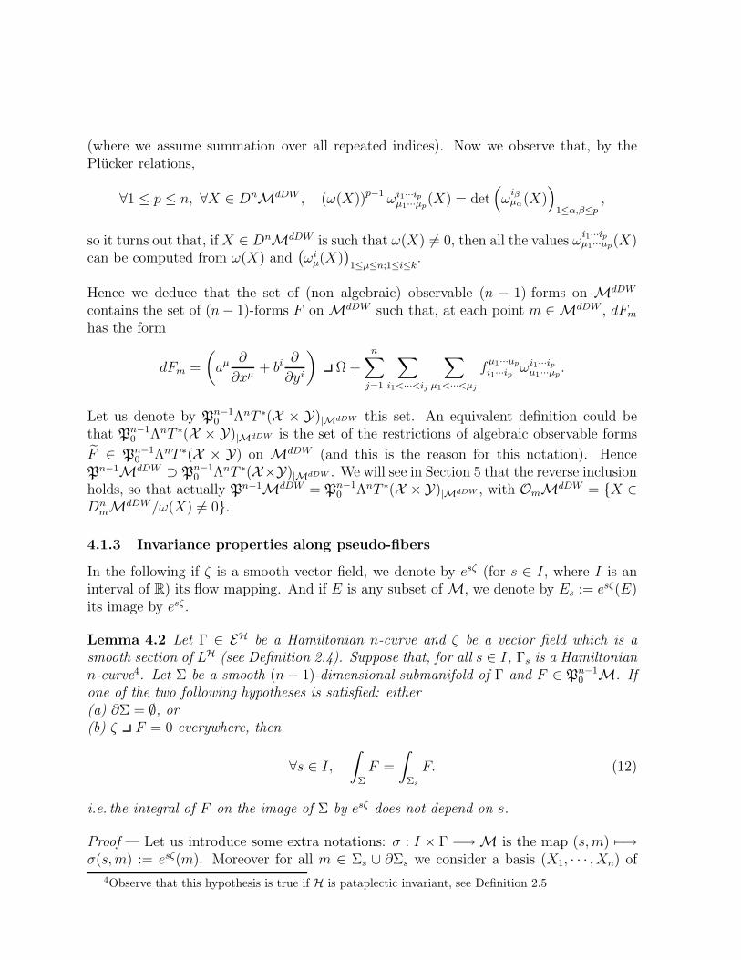
4.1.3 Invariance properties along pseudo-fibers

In the following if ζ is a smooth vector field, we denote by esζ (for s ∈ I, where I is aninterval of R) its flow mapping. And if E is any subset of M, we denote by Es := esζ(E)its image by esζ .

Lemma 4.2 Let Γ ∈ EH be a Hamiltonian n-curve and ζ be a vector field which is asmooth section of LH (see Definition 2.4). Suppose that, for all s ∈ I, Γs is a Hamiltoniann-curve4. Let Σ be a smooth (n− 1)-dimensional submanifold of Γ and F ∈ Pn−1

0 M. Ifone of the two following hypotheses is satisfied: either(a) ∂Σ = ∅, or(b) ζ F = 0 everywhere, then

∀s ∈ I,

∫

Σ

F =

∫

Σs

F. (12)

i.e. the integral of F on the image of Σ by esζ does not depend on s.

Proof — Let us introduce some extra notations: σ : I × Γ −→ M is the map (s,m) 7−→σ(s,m) := esζ(m). Moreover for all m ∈ Σs ∪ ∂Σs we consider a basis (X1, · · · , Xn) of

4Observe that this hypothesis is true if H is pataplectic invariant, see Definition 2.5

L H

Γ

Σ

Σ

Γ

s s

Figure 1: Invariance of an observable functional along the generalized pseudofiber directions as inLemma 4.2

TmΓs such that X := X1 ∧ · · · ∧ Xn ∈ [X]Hm, (X2, · · · , Xn) is a basis of TmΣs and, ifm ∈ ∂Σs, (X3, · · · , Xn) is a basis of Tm∂Σs. Lastly we let (θ1, · · · , θn) be a basis of T ∗

mΓs,dual of (X1, · · · , Xn). We first note that

∫

(0,s)×∂Σ

σ∗F = 0,

either because ∂Σ = ∅ (a) or because, if ∂Σ 6= ∅, this integral is equal to∫

(0,s)×∂Σ

Fσ(s,m)(ζ,X3, · · · , Xn)ds ∧ θ3 ∧ · · · ∧ θn

which vanishes by (b). Thus∫

Σs

F −

∫

Σ

F =

∫

Σ

(esζ)∗F − F =

∫

Σ

(esζ)∗F − F −

∫

(0,s)×∂Σ

σ∗F

=

∫

∂((0,s)×Σ)

σ∗F =

∫

(0,s)×Σ

d (σ∗F )

=

∫

(0,s)×Σ

σ∗dF =

∫

σ((0,s)×Σ)

dFσ(s,m)(ζ,X2, · · · , Xn)ds ∧ θ2 ∧ · · · ∧ θn.

But since F ∈ Pn−10 M, we have that

dFσ(s,m)(ζ,X2, · · · , Xn) = −Ω(ξF , ζ, X2, · · · , Xn)= Ω(ζ, ξF , X2, · · · , Xn)= 〈ξF ∧X2 ∧ · · · ∧Xn, ζ Ω〉.

Now the key observation is that ξF ∧X2 ∧ · · · ∧Xn ∈ TXDnmM and so the hypothesis of

the Lemma implies that 〈ξF ∧X2 ∧ · · · ∧Xn, ζ Ω〉 = 0. Hence (12) is satisfied.

Example 6 — Algebraic observable (n−1)-forms satisfying the assumption (b) in Lemma4.2 — If M = ΛnT ∗N and if H is a Legendre image Hamiltonian then any (n− 1)-formF of the type F = ξ θ, where ξ is a vector field on N , is algebraic observable (see [13],

[7]). But as pointed out in Section 2.2 (definition 2.4) since LHm ⊂ KerdΠm any vector

field ζ which is a section of LH is necessarily “vertical” and satisfies ζ θ = 0. Henceζ F = 0. Such (n − 1)-forms ξ θ correspond to components of the momentum andthe energy-momentum of the field (see [13]).

4.1.4 Poisson brackets between observable (n− 1)-forms

There is a natural way to construct a Poisson bracket ·, · : Pn−10 M × Pn−1

0 M 7−→Pn−1

0 M. To each algebraic observable forms F,G ∈ Pn−10 M we associate first the vector

fields ξF and ξG such that ξF Ω + dF = ξG Ω + dG = 0 and then the (n− 1)-form

F,G := ξF ∧ ξG Ω.

It can be shown (see [13]) that F,G ∈ Pn−10 M and that

dF,G + [ξF , ξG] Ω = 0,

where [·, ·] is the Lie bracket on vector fields. Moreover this bracket satisfies the Jacobicondition modulo an exact term5 (see [13])

F,G, H+ G,H, F+ H,F, G = d(ξF ∧ ξG ∧ ξH Ω).

As an application of this definition, for any slice Σ of codimension 1 we can define aPoisson bracket between the observable functionals

∫ΣF and

∫ΣG by ∀Γ ∈ EH,

∫

Σ

F,

∫

Σ

G

(Γ) :=

∫

Σ∩Γ

F,G.

If ∂Γ = ∅, it is clear that this Poisson bracket satisfies the Jacobi identity. Computationsin [22], [20], [13] show that this Poisson bracket coincides with the Poisson bracket of thestandard canonical formalism used for quantum field theory.

One can try to extend the bracket between forms in Pn−10 M to forms in Pn−1M through

different strategies:

• By exploiting the relation

F,G = ξF dG = −ξG dF,

which holds for all F,G ∈ Pn−10 M. A natural definition is to set:

∀F ∈ Pn−10 M, ∀G ∈ Pn−1M, F,G = −G,F := ξF dG.

In [13] we call this operation an external Poisson bracket.5Note that in case where the multisymplectic manifold (M, Ω) is exact in the sense of M. Forger,

C. Paufler and H. Romer [7], i.e. if there exists an n-form θ such that Ω = dθ (beware that our signconventions differ with [7]), an alternative Poisson bracket can be defined:

F, Gθ := F, G + d(ξG F − ξF G + ξF ∧ ξG θ).

Then this bracket satisfies the Jacobi identity (in particular with a right hand side equal to 0), see [6],[7].

• If we know that there is an embedding ι : M −→ M, into a higher dimensionalpataplectic manifold (M, Ω), and that (i) Pn−1

0 M = Pn−1M, (ii) the pull-back

mapping Pn−10 M −→ Pn−1M : F 7−→ ι∗F is — modulo the set of closed (n − 1)-

forms on M which vanish on M — an isomorphism. Then there exists a uniquePoisson bracket on Pn−1M which is the image of the Poisson bracket on Pn−1

0 M.This situation is achieved for instance if M is a submanifold of ΛnT ∗N , a situa-tion which arises after a Legendre transform. This will lead basically to the samestructure as the external Poisson bracket. In more general cases the question ofextending M into M is relatively subtle and is discussed in the paper [17].

4.2 Algebraic observable (p− 1)-forms

It is worth to ask about the relevant definition of algebraic observable (p − 1)-forms.Indeed a first possibility is to generalize directly Definition 4.1: we would say that the(p − 1)-form F is algebraic observable if there exists a (1 + n − p)-multivector field ξFsuch that dF + ξF Ω = 0. Note that in this case ξF is not unique in general. Thisapproach has been proposed by I. Kanatchikov in [20] and [21]. It allows us to definea nice notion of Poisson bracket between such forms and leads to a structure of gradedLie algebra. However this definition has not good dynamical properties and in particularthere is no analogue of Theorem 3.1 for such forms. In other words our definition 3.3of (non algebraic) observable (p − 1)-forms results from the search for the more generalhypothesis for Theorem 3.1 to be true, but (p− 1)-forms which are observable accordingto Kanatchikov are not observable in the sense of our Definition 3.3. Here we preferto privilege the dynamical properties instead trying to generalize Noether’s theorem to(p− 1)-forms.

4.2.1 Definitions and basic properties

We simply adapt Definitions 3.2, 3.3 and 3.4 by replacing P nT ∗mM of Definition 3.1 by

its subset P n0 T

∗mM of Definition 4.1: it leads to the notions of algebraic copolarization

P ∗0 T

∗M, of the set Pp−10 M of algebraic observable (p − 1)-forms and of algebraic

polarization P ∗0 TM. Of course in the case of a pataplectic manifold algebraic and non

algebraic notions coincide.

A consequence of these definitions is that for any 1 ≤ p ≤ n, for any algebraic observable(p − 1)-forms F ∈ P

p−10 M and for any φ ∈ P n−p

0 T ⋆mM, there exists a unique vectorξF (φ) ∈ TmM such that φ ∧ dF + ξF (φ) Ω = 0. We thus obtain a linear mapping

ξF : P n−p0 T ⋆mM −→ TmM

φ 7−→ ξF (φ).(13)

Hence we can associate to F the tensor field ξF . By duality between P n−p0 T ⋆mM and

P n−p0 TmM, ξF can also be identified with a section of the bundle P n−p

0 TM⊗M TM.

Moreover an alternative definition of the pseudobracket (see Definition 3.5) can be givenusing the tensor field ξF defined by (13).

Lemma 4.3 For any Hamiltonian function H and any F ∈ Pp−10 M, we have

H, F = −ξF dH, (14)

where the right hand side is the section of P n−p0 TM defined by

〈ξF dH, φ〉 := ξF (φ) dH, ∀φ ∈ P n−p0 T ⋆M. (15)

Proof — Starting from Definition 3.5, we have ∀φ ∈ P n−p0 T ⋆M,

〈H, F, φ〉 = (−1)(n−p)p〈[X]H dF, φ〉= (−1)(n−p)p〈[X]H, dF ∧ φ〉= 〈[X]H, φ ∧ dF 〉= −〈[X]H, ξF (φ) Ω〉= −(−1)nξF (φ) [X]H Ω= −ξF (φ) dH.

The price we have to pay is that the notion of Poisson bracket between (p − 1)-forms isnow a much more delicate task than in the framework of Kanatchikov. This question isthe subject of the next paragraph.

4.2.2 Brackets between algebraic observable (p− 1)-forms

We now consider algebraic observable (p−1)-forms for 1 ≤ p ≤ n and discuss the possibil-ity of defining a Poisson bracket between these observable forms, which could be relevantfor quantization. This is slightly more delicate than for forms of degree n − 1 and thedefinitions proposed here are based on empirical observations. We first assume a furtherhypothesis on the copolarization (which is satisfied on ΛnT ∗N ).

We first recall a definition which was given in [15]: given any X = X1 ∧ · · · ∧Xn ∈ DnmM

and any form a ∈ T ∗mM we will write that a|X 6= 0 if and only if (a(X1), · · · , a(Xn)) 6= 0.

We will say that a function f ∈ C1(M,R) is 1-regular if and only if we have

∀m ∈ M, ∀X ∈ [X]Hm, dfm|X 6= 0. (16)

Hypothesis on P10M — We suppose that any 1-regular function f ∈ C1(M,R) satisfies6

(i) f ∈ P10M

(ii) For all infinitesimal symplectomorphism ξ ∈ sp0M, ξ df = 0.

6these assumptions are actually satisfied in Pn−1M

Now let 1 ≤ p, q ≤ n and F ∈ Pp−10 M and G ∈ P

q−10 M and let us analyze what condi-

tion should satisfy the bracket F,G. We will consider smooth functions f 1, · · · , fn−p,g1, · · · , gn−q and t on M. We assume that all these functions are 1-regular and thatdf 1m ∧ · · · ∧ dfn−pm ∧ dg1

m ∧ · · · ∧ dgn−qm 6= 0. Then, because of hypothesis (i),

F := df 1 ∧ · · · ∧ dfn−p ∧ F, G := dg1 ∧ · · · ∧ dgn−q ∧G ∈ Pn−10 M.

Lastly let Γ be a Hamiltonian n-curve and Σ be a level set of t. Then∫

Σ

F ,

∫

Σ

G

(Γ) =

(∫

Σ

F , G

)(Γ) =

∫

Σ∩Γ

F , G

. (17)

We now suppose that the functions f := (f 1, · · · , fn−p) and g := (g1, · · · , gn−q) concentratearound submanifolds denoted respectively by γf and γg of codimension n − p and n − qrespectively. More precisely we suppose that df 1 ∧ · · · ∧ dfn−p (resp. dg1 ∧ · · · ∧ dgn−q) iszero outside a tubular neighborhood of γf (resp. of γg) of width ε and that the integral ofdf 1 ∧ · · · ∧ dfn−p (resp. dg1 ∧ · · · ∧ dgn−q) on a disc submanifold of dimension n− p (resp.n − q) which cuts transversally γf (resp. γg) is equal to 1. Moreover we suppose thatγf and γg cut transversally Σ ∩ Γ along submanifolds denoted by γf and γg respectively.Then, as ε→ 0, we have∫

Σ∩Γ

df 1 ∧ · · · ∧ dfn−p ∧ F →

∫

Σ∩γf∩Γ

F,

∫

Σ∩Γ

dg1 ∧ · · · ∧ dgn−q ∧G→

∫

Σ∩γg∩Γ

G.

This tells us that the left hand side of (17) is an approximation for∫

Σ∩γf

F,

∫

Σ∩γg

G

(Γ).

We now want to compute what is the limit of the right hand side of (17). Using thehypothesis (ii) we have

F , G = ξF d (dg1 ∧ · · · ∧ dgn−q ∧G)= (−1)n−qξ

Fdg1 ∧ · · · ∧ dgn−q ∧ dG

= dg1 ∧ · · · ∧ dgn−q ∧(ξF

dG).

And we have similarly:

F , G = −df 1 ∧ · · · ∧ dfn−p ∧(ξG

dF).

We now use the following result.

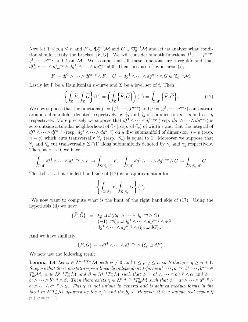
Lemma 4.4 Let φ ∈ Λn−1T ∗mM with φ 6= 0 and 1 ≤ p, q ≤ n such that p + q ≥ n + 1.

Suppose that there exists 2n−p−q linearly independent 1-forms a1, · · · , an−p, b1, · · · , bn−q ∈T ∗mM, α ∈ Λp−1T ∗

mM and β ∈ Λq−1T ∗mM such that φ = a1 ∧ · · · ∧ an−p ∧ α and φ =

b1 ∧ · · · ∧ bn−q ∧ β. Then there exists χ ∈ Λp+q−n−1T ∗mM such that φ = a1 ∧ · · · ∧ an−p ∧

b1 ∧ · · · ∧ bn−q ∧ χ. This χ is not unique in general and is defined modulo forms in theideal in Λ∗T ∗

mM spanned by the aj’s and the bj’s. However it is a unique real scalar ifp+ q = n + 1.

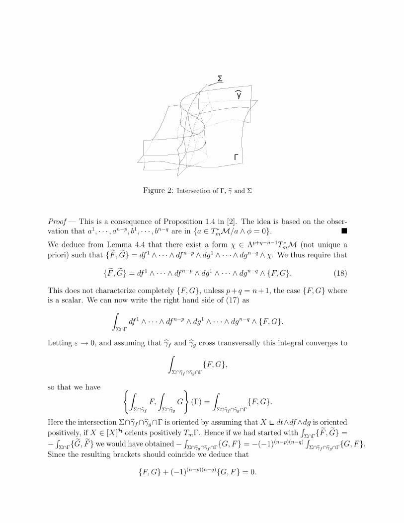
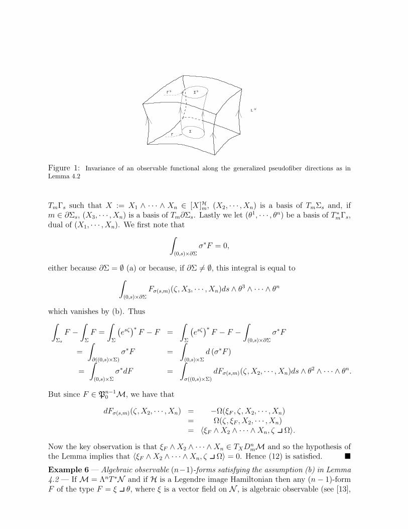
Γ

γ

Σ

Figure 2: Intersection of Γ, γ and Σ

Proof — This is a consequence of Proposition 1.4 in [2]. The idea is based on the obser-vation that a1, · · · , an−p, b1, · · · , bn−q are in a ∈ T ∗

mM/a ∧ φ = 0.

We deduce from Lemma 4.4 that there exist a form χ ∈ Λp+q−n−1T ∗mM (not unique a

priori) such that F , G = df 1 ∧ · · · ∧ dfn−p ∧ dg1 ∧ · · · ∧ dgn−q ∧ χ. We thus require that

F , G = df 1 ∧ · · · ∧ dfn−p ∧ dg1 ∧ · · · ∧ dgn−q ∧ F,G. (18)

This does not characterize completely F,G, unless p+ q = n+1, the case F,G whereis a scalar. We can now write the right hand side of (17) as

∫

Σ∩Γ

df 1 ∧ · · · ∧ dfn−p ∧ dg1 ∧ · · · ∧ dgn−q ∧ F,G.

Letting ε → 0, and assuming that γf and γg cross transversally this integral converges to

∫

Σ∩γf∩γg∩Γ

F,G,

so that we have ∫

Σ∩γf

F,

∫

Σ∩γg

G

(Γ) =

∫

Σ∩γf∩γg∩Γ

F,G.

Here the intersection Σ∩γf∩γg∩Γ is oriented by assuming thatX dt∧df∧dg is oriented

positively, if X ∈ [X]H orients positively TmΓ. Hence if we had started with∫Σ∩Γ

F , G =

−∫Σ∩Γ

G, F we would have obtained −∫Σ∩γg∩γf∩Γ

G,F = −(−1)(n−p)(n−q)∫Σ∩γf∩γg∩Γ

G,F.

Since the resulting brackets should coincide we deduce that

F,G + (−1)(n−p)(n−q)G,F = 0.

Conclusion — In two cases we can guess a more direct definition of F,G. First whenone of the two forms F or G is in Pn−1

0 M, let us say F ∈ Pp−10 M and G ∈ Pn−1

0 M: thenwe let

F,G := −ξG dF. (19)

This is the idea of external bracket as in Paragraph 4.1.4. We remark that if f 1, · · · , fn−p

are in P10M and are such that ξG df 1∧· · ·∧dfn−p = 0, then df 1∧· · ·∧dfn−p∧F ∈ Pn−1

0 Mand

df 1 ∧ · · · ∧ dfn−p ∧ F,G = df 1 ∧ · · · ∧ dfn−p ∧ F,G

so that the requirement (18) is satisfied.

Second if F ∈ Pp−10 M, G ∈ P

q−10 M, where 1 < p, q < n and p+ q = n + 1: then F,G

is just a scalar and so is characterized by (18).

Example 7 — Sigma models — Let M := ΛnT ⋆(X × Y) as in Section 2. For simplicitywe restrict ourself to the de Donder–Weyl submanifold MdDW (see Section 2.3), so thatthe Poincare-Cartan form is θ = eω+ pµi dy

i∧ωµ and the multisymplectic form is Ω = dθ.Let φ be a function on X and consider the observable 0-form yi (for 1 ≤ i ≤ k) and theobservable (n − 1)-form Pj,φ := φ(x)∂/∂yj θ. Then ξPj,φ

= φ∂/∂yj − pµj (∂φ/∂xµ) ∂/∂eand thus Pj,φ, yi = ξPj,φ

dyi = δijφ. It gives the following bracket for observablefunctionals

∫

Σ

Pj,φ,

∫

Σ∩γ

yi

(Γ) =

∫

Σ∩γ∩Γ

δijφ(x) = δij∑

m∈Σ∩γ∩Γ

sign(m)φ(m),

where Σ, γ and Γ are supposed to cross transversally and sign(m) accounts for the orien-tation of their intersection points.

Example 4” — Maxwell equations — In this case we find that, for all functions f, g1, g2 :MMax −→ R whose differentials are proper on Om, df ∧π, dg1∧dg2∧a = df ∧dg1∧dg2.We hence deduce that π, a = 1: these forms are canonically conjugate. We deduce thefollowing bracket for observable functionals

∫

Σ∩γf

π,

∫

Σ∩γg

a

(Γ) =

∑

m∈Σ∩γf∩γg∩Γ

sign(m),

where Σ ∩ γf ∩ Γ is a surface and Σ ∩ γg ∩ Γ is a curve in the three-dimensional spaceΣ ∩ Γ. Note that this conclusion was achieved by I.Kanatchikov with its definition ofbracket π, aKana := ξπ da, where ξπ ∈ Λ2T ∗

mMMax is such that ξπ Ω = dπ. But

there by choosing ξπ = (1/2)∑

µ(∂/∂aµ) ∧ (∂/∂xµ) one finds (in our convention) thatπ, aKana = n/2 (= 2, if n = 4). So the two brackets differ (the new bracket in thispaper differs also from the one that we proposed in [13]).

5 The case of ΛnT ⋆N

We will here study algebraic and non algebraic observable (n − 1)-forms in ΛnT ⋆N andprove in particular that ΛnT ⋆N is pataplectic. This part can be seen as a complementof an analysis of other properties of ΛnT ⋆N given in [15]. In particular we use thesame notations: since we are interested here in local properties of M, we will use localcoordinates m = (q, p) = (qα, pα1···αn

) on M, and the multisymplectic form reads Ω =∑α1<···<αn

dpα1···αn∧ dqα1 ∧ · · · ∧ dqαn . For m = (q, p), we write

dqH :=∑

1≤α≤n+k

∂H

∂qαdqα, dpH :=

∑

1≤α1<···<αn≤n+k

∂H

∂pα1···αn

dpα1···αn,

so that dH = dqH + dpH.

5.1 Algebraic and non algebraic observable (n−1)-forms coincide

We show here that (ΛnT ⋆N ,Ω) is a pataplectic manifold.

Theorem 5.1 If M is an open subset of ΛnT ⋆N , then Pn−10 M = Pn−1M.

Proof — We already know that Pn−10 M ⊂ Pn−1M. Hence we need to prove the reverse

inclusion. So in the following we consider some m ∈ M and a form a ∈ P nmM and

we will prove that there exists a vector field ξ on M such that a = ξ Ω. We writeOmM := Oa

mM.

Step 1 — We show that given m = (q, p) ∈ M it is possible to find n + k vectors

(Q1, · · · , Qn+k) of TmM such that, if Π∗(Qα) =: Qα (the image of Qα by the mapΠ : M −→ N ), then (Q1, · · · , Qn+k) is a basis of TqN and ∀(α1, · · · , αn) s.t. 1 ≤ α1 <

· · · < αn ≤ n + k, Qα1∧ · · · ∧ Qαn

∈ OmM.

This can be done by induction by using the fact that OmM is dense in DnmM. We

start from any family of vectors (Q01, · · · , Q

0n+k) of TmM such that (Q0

1, · · · , Q0n+k) is a

basis of TqN (where Q0α := Π∗(Q

0α)). We then order the (n+k)!

n!k!multi-indices (α1, · · · , αn)

such that 1 ≤ α1 < · · · < αn ≤ n + k (using for instance the dictionary rule). Using

the density of OmM we can perturb slightly (Q01, · · · , Q

0n+k) into (Q1

1, · · · , Q1n+k) in such

a way that for instance Q11 ∧ · · · ∧ Q1

n ∈ OmM (assuming that (1, · · · , n) is the small-

est index). Then we perturb further (Q11, · · · , Q

1n+k) into (Q2

1, · · · , Q2n+k) in such a way

that Q21 ∧ · · · ∧ Q2

n−1 ∧ Q2n+1 ∈ OmM (assuming that (1, · · · , n − 1, n + 1) is the next

one). Using the fact that OmM is open we can do it in such a way that we still have

Q21 ∧ · · · ∧ Q2

n ∈ OmM. We proceed further until the conclusion is reached.

In the following we choose local coordinates around m in such a way that Qα = ∂α +∑1≤α1<···<αn≤n+k Pα,α1···αn

∂α1···αn .

Step 2 — We choose a multi-index (α1, · · · , αn) with 1 ≤ α1 < · · · < αn ≤ n + k anddefine the set Oα1···αn

m M := OmM∩Dα1···αnm M, where

Dα1···αn

m M :=

X1 ∧ · · · ∧Xn ∈ Dn

mM/∀µ,Xµ =∂

∂qαµ+

∑

1≤β1<···<βn≤n+k

Xµ,β1···βn

∂

∂pβ1···βn

.

We want to understand the consequences of the relation

∀X, X ∈ Oα1···αn

m M, X Ω = X Ω =⇒ a(X) = a(X). (20)

Note that Oα1···αnm M is open and non empty (since by the previous step, Qα1

∧· · ·∧Qαn∈

Oα1···αnm M). We also observe that, on Dα1···αn

m M, X 7−→ X Ω and X 7−→ a(X) arerespectively an affine function and a polynomial function of the coordinates variablesXµ,β1···βn

. Thus the following result implies that actually Oα1···αnm M = Dα1···αn

m M.

Lemma 5.1 Let N ∈ N and let P be a polynomial on RN and f1, · · · , fp be affine functionson RN . Assume that there exists some x0 ∈ RN and a neighborhood V0 of x0 in RN suchthat

∀x, x ∈ V0, if ∀j = 1, · · · , p, fj(x) = fj(x), then P (x) = P (x).

Then this property is true on RN .

Proof — We can assume without loss of generality that the functions fj are linear andalso choose coordinates on RN such that fj(x) = xj , ∀j = 1, · · · , p. Then the assumptionmeans that, on V0, P does not depend on xp+1, · · ·xN . Since P is a polynomial wededuce that P is a polynomial on the variables x1, · · · , xp and so the property is trueeverywhere.

Step 3 — Without loss of generality we will also assume in the following that (α1, · · · , αn) =(1, · · · , n) for simplicity. We shall denote by mI all coordinates qα and pα1···αn

, so that wecan write

a =∑

I1<···<In

AI1···IndmI1 ∧ · · · ∧ dmIn.

We will prove that if (I1, · · · , In) is a multi-index such that

• mI1, · · · , mIn contains at least two distinct coordinates of the type pα1···αnand

• mI1, · · · , mIn does not contain any qα, for n + 1 ≤ α ≤ n+ k

then AI1···In = 0. Without loss of generality we can suppose that ∃p ∈ N such that1 ≤ p ≤ n− 2 and

mI1 = q1, · · · , mIp = qp and mIp+1, · · · , mIn ∈ pα1···αn/1 ≤ α1 < · · · < αn ≤ n + k.

We test property (20) specialized to the case where X = X1 ∧ · · · ∧Xn with

Xµ =∂

∂qµ+

n∑

j=p+1

XIjµ

∂

∂mIj, ∀µ = 1, · · · , n.

Then

a(X) = AI1···In

∣∣∣∣∣∣∣∣∣∣∣∣∣∣

1 · · · 0 0 · · · 0...

. . ....

......

0 · · · 1 0 · · · 0

XIp+1

1 · · · XIp+1

p XIp+1

p+1 · · · XIp+1

n

......

......

XIn1 · · · XIn

p XInp+1 · · · XIn

n

∣∣∣∣∣∣∣∣∣∣∣∣∣∣

= AI1···In

∣∣∣∣∣∣∣

XIp+1

p+1 · · · XIp+1

n

......

XInp+1 · · · XIn

n

∣∣∣∣∣∣∣.

(21)Note that we can write any X ∈ D1···n

m M as X = X1 ∧ · · · ∧Xn with

Xµ =∂

∂qµ+ Eµ

∂

∂p1···n+

n+k∑

β=n+1

Mµ,β +Rµ,

where Mµ,β :=∑n

ν=1(−1)n+νMνµ,β∂

1···ν···nβ and Rµ :=∑

(α1,···,αn)∈I∗∗ Xµ,α1···αn∂α1···αn . And

then

(−1)nX Ω = dp1···n −n∑

µ=1

Eµdqµ −

n+k∑

β=n+1

(n∑

µ=1

Mµµ,β

)dqβ.

Within our specialization this leads to the following key observation7: at most one line(X

Ij1 , · · · , X

Ijn ) ( for p+1 ≤ j ≤ n) in the n×n determinant in (21) is a function of X Ω

(for mIj = p1···n). In all other lines number ν, where p + 1 ≤ ν ≤ n and ν 6= j, there isat most one component XIν

µ which is a function of X Ω. All the other components areindependent of X Ω. Thus we have the following alternative.

(i) mIp+1, · · · , mIn does not contain p1···n (i.e. the line (E1, · · · , En) does not appearin the n× n determinant in (21)), or

(ii) mIp+1, · · · , mIn contains p1···n (i.e. one of the lines is (E1, · · · , En))

Case (i) — Then the right hand side determinant in (20) is a polynomial of degree

n− p ≥ 2. Thus we can find a monomial in this determinant of the form XIp+1

σ(p+2) · · ·XInσ(n)

(where σ is a substitution of p+1, · · · , n) where each variable is independent of X Ω.Hence in order to achieve (20) we must have AI1···In = 0.

Case (ii) — We assume w.l.g. that mIp+1 = p1···n. We freeze the variables XIp+1

µ (i.e.Eµ)

suitably and specialize again property (20) by letting free only the variables XIjµ for

p + 2 ≤ j ≤ n and 1 ≤ µ ≤ n. Two subcases occur: if p < n − 2 then we chooseXIp+1

µ = δp+1µ . Then we are reduced to a situation quite similar to the first case and we

can conclude using the same argument (this time with a determinant which is a monomialof degree n− 1 − p ≥ 2).

If p = n − 2 then a(X) = AI1···In

(XInn X

In−1

n−1 −XInn−1X

In−1

n

). If the knowledge of X Ω

7Remark that each of the n− p last lines in the n× n determinant in (21) is either (E1, · · · , En) or ofthe type (Mν

1,β, · · · , Mνm,β) or (X1,α1···αn

, · · · , Xn,α1···αn), for (α1, · · · , αn) ∈ I∗∗.

prescribes XInn then by the key observation XIn

n−1 is free and by choosing XIn−1

µ = δnµ we

obtain a(X) = −AI1···InXInn−1. If X Ω prescribes XIn

n−1 then XInn is free and by choosing

XIn−1

µ = δn−1µ we obtain a(X) = AI1···InX

Inn . In both cases we must have AI1···In = 0 in

order to have (20).

Conclusion — Steps 2 and 3 show that, on O1···nm M, X 7−→ a(X) is an affine function

on the variables Xµ,β1···βn. Then by standard results in linear algebra (20) implies that,

∀X ∈ O1···nm M, a(X) is an affine combination of the components of X Ω. By repeating

this step on each Oα1···αnm M we deduce the conclusion.

Theorem 5.2 Assume that N = X × Y, M = ΛnT ∗N and consider MdDW to be thesubmanifold of ΛnT ∗N as defined in Paragraph 2.3.1 equipped with the multisymplecticform ΩdDW which is the restriction of Ω to MdDW . Then Pn−1MdDW coincides withPn−1

0 ΛnT ∗(X ×Y)|MdDW , the set of the restrictions of algebraic observable (n− 1)-formsof (M,Ω) to MdDW .

Proof — The fact that PnMdDW contains all the restrictions of algebraic observable(n − 1)-forms of (M,Ω) to MdDW was observed in Paragraph 4.2.1. The proof of thereverse inclusion follows the same strategy as the proof of Theorem 5.1 and is left to thereader.

5.2 All algebraic observable (n− 1)-forms

We conclude this section by giving the expression of all algebraic observable (n−1)-formson an open subset of ΛnT ⋆N . For details see [15]. First the general expression of aninfinitesimal symplectomorphism is Ξ = χ + ξ, where

χ :=∑

β1<···<βn

χβ1···βn(q)

∂

∂pβ1···βn

and ξ :=∑

α

ξα(q)∂

∂qα−∑

α,β

∂ξα

∂qβ(q)Πβ

α, (22)

and where the coefficients χβ1···βnare so that d(χ Ω) = 0, ξ :=

∑α ξ

α(q) ∂∂qα is an arbi-

trary vector field on N , and Πβα :=

∑β1<···<βn

∑µ δ

ββµpβ1···βµ−1αβµ+1···βn

∂∂pβ1···βn

.

As a consequence any algebraic observable (n−1)-form F can be written as F = Qζ +Pξ,where

Qζ =∑

β1<···<βn−1

ζβ1···βn−1(q)dqβ1 ∧ · · · ∧ dqβn−1 and Pξ = ξ θ.

Then χ Ω = −dQζ and ξ Ω = −dPξ.Lastly we let8 spQM to be the set of infinitesimal symplectomorphisms of the form χ

(with χ Ω closed) and spPM those of the form ξ (for all vector fields ξ ∈ Γ(M, TM))as defined in (22). Then one can observe that sp0M = spPM ⋉ spQM (see [14]).

8recall that sp0M is the set of all symplectomorphisms of (M, Ω) (see Definition 2.3)

6 Dynamical observable forms and functionals

One question is left: to make sense of the Poisson bracket of two observable functionalssupported on different slices. This is essential in an Einstein picture (classical analogue ofthe Heisenberg picture) which seems unavoidable in a completely covariant theory. Onepossible answer rests on the notion of dynamical observable forms (in contrast with kine-matic observable functionals). To be more precise let Σ and Σ′ be two different slices ofcodimension 1 and F and G be two algebraic observable (n− 1)-forms and let us try todefine the Poisson bracket between

∫ΣF and

∫Σ′ G.

One way is to express one of the two observable functionals, say∫Σ′ G, as an integral over

Σ. This can be achieved for all slices Σ and Σ′ which are cobordism equivalent, i.e. suchthat there exists a smooth domain D in M with ∂D = Σ′ −Σ, and if dG|Γ = 0, ∀Γ ∈ EH.Then indeed ∫

Σ∩Γ

G−

∫

Σ′∩Γ

G =

∫

∂D∩Γ

G =

∫

D∩Γ

dG = 0, (23)

so that ∫

Σ′

G =

∫

Σ

G on EH.

Thus we are led to the following.

Definition 6.1 A dynamical observable (n−1)-form is an observable form G ∈ Pn−1Msuch that

H, G = 0

Indeed Corollary 3.1 implies immediately that if G is a dynamical observable (n−1)-formthen dG|Γ = 0 and hence (23) holds. As a consequence if F is any observable (n−1)-formand G is a dynamical observable (n − 1)-form (and if one of both is an algebraic one),then we can state ∫

Σ

F,

∫

Σ′

G

:=

∫

Σ

F,

∫

Σ

G

.

The concept of dynamical observable form is actually more or less the one used by J.Kijowski in [22], since his theory corresponds to working on the restriction of (M,Ω) onthe hypersurface H = 0.

Hence we are led to the question of characterizing dynamical observable (n − 1)-forms.(We shall consider mostly algebraic observable forms.) This question was already in-vestigated for some particular case in [22] (and discussed in [10]) and the answer was a(surprising) deception: as long as the variational problem is linear (i.e. the Lagrangianis a quadratic function of all variables) there are many observable functionals (basicallyall smeared integrals of fields using test functions which satisfy the Euler-Lagrange equa-tion), but as soon as the problem is non linear the choice of dynamical observable formsis dramatically reduced and only global dynamical observable exists. For instance for a

non nonlinear scalar field theory with L(u, du) = 12(∂tu)

2 − |∇u|2 + m2

2u2 + λ

3u3, the only

dynamical observable forms G are those for which ξG is a generator of the Poincare group.One can also note that in general dynamical observable forms correspond to momentumor energy-momentum observable functionals.

Several possibilities may be considered to go around this difficulty. If the variationalproblem can be seen as a deformation of a linear one (i.e. of a free field theory) then itcould be possible to construct a perturbation theory, leading to Feynman type expansionsfor classical fields. For an example of such a theory, see [12] and [11]. Another interestingdirection would be to explore completely integrable systems. We present here a thirdalternative, which relies on symmetries and we will see on a simple example how thepurpose of constructing dynamical observable forms leads naturally to gauge theories.

Example 8 — Complex scalar fields — We consider on the set of maps ϕ : Rn −→ C thevariational problem with Lagrangian

L0(ϕ, dϕ) =1

2ηµν

∂ϕ

∂xµ∂ϕ

∂xν+ V

(|ϕ|2

2

)=

1

2ηµν(∂ϕ1

∂xµ∂ϕ1

∂xν+∂ϕ2

∂xµ∂ϕ2

∂xν

)+ V

(|ϕ|2

2

).

Here ϕ = ϕ1 + iϕ2. We consider the multisymplectic manifold M0, with coordinates xµ,φ1, φ2, e, pµ1 and pµ2 and the multisymplectic form Ω0 = de∧ ω+ dpµa ∧ dφ

a ∧ ωµ (which isthe differential of the Poincare-Cartan form θ0 := eω+pµadφ

a∧ωµ). Then the Hamiltonianis

H0(x, φ, e, p) = e+1

2ηµν(p

µ1p

ν1 + pµ2p

ν2) − V

(|φ|2

2

).

We look for (n− 1)-forms F0 on M0 such that

dF0 + ξF0Ω0 = 0, for some vector field ξF0

, (24)

dH0(ξF0) = 0. (25)

The analysis of this problem can be dealt by looking for all vector fields

ξ0 = Xµ(x, φ, e, p)∂

∂xµ+ Φa(x, φ, e, p)

∂

∂φa+ E(x, φ, e, p)

∂

∂e+ P µ

a (x, φ, e, p)∂

∂pµa.

satisfying (24) and (25). For simplicity we will assume that Xµ = 0 (this will excludestress-energy tensor observable forms Xµ ∂

∂xµ θ0, for Xµ constant). Then we find twocases:

If V (|φ|2/2) is quadratic in φ, i.e. if V (|φ|2/2) = m2|φ|2/2, then Equations (24) and (24)have the solutions

ξ0 = λ~j0 + Ua(x)∂

∂φa−

(pµa∂Ua

∂xµ(x) + δabLU

a(x)φb)∂

∂e+ ηµνδab

∂Ua

∂xµ(x)

∂

∂pµb,

where λ is a real constant,

~j0 :=

(φ2 ∂

∂φ1− φ1 ∂

∂φ2

)+

(pµ2

∂

∂pµ1− pµ1

∂

∂pµ2

),

L := −ηµν ∂2

∂xµ∂xν and U1 and U2 are arbitrary solutions of the linear equation LU+m2U =

0. Then F0 = Uapµaωµ − ηµν(∂U1

∂xν φ1 + ∂U2

∂xν φ2)ωµ + λ (pµ1φ

2 − pµ2φ1)ωµ.

However if V ′ is not a constant, then system (24) and (24) has only the solutions ξ0 = λ~j0and the resulting dynamical observable (n − 1)-form is F0 = λ(pµ1φ

2 − pµ2φ1)ωµ, which

corresponds to the global charge due to the U(1) invariance of the Lagrangian.

For instance we would like to replace λ by a smooth function ψ of x, i.e. to look atF = ψ(x)(pµ1φ

2 − pµ2φ1)ωµ. These are non dynamical algebraic observable (n − 1)-

forms since we have dF1 + ξ Ω0 = 0, where ξ := ψ~j0 − (pµ1φ2 − pµ2φ

1) ∂ψ∂xµ

∂∂e

, but

dH0(ξ) = −(pµ1φ2 − pµ2φ

2) ∂ψ∂xµ 6= 0.

Now in order to enlarge the set of dynamical observable forms, an idea is to furtherincorporate the gauge potential field A := Aµdx

µ and consider the Lagrangian

L1(ϕ,A, dϕ) :=1

2ηµν(∂ϕ

∂xµ+ iAµϕ

)(∂ϕ

∂xν+ iAνϕ

)−

1

4ηµληνσFµνFλσ + V

(|ϕ|2

2

),

where Fµν := ∂Aν

∂xµ − ∂Aµ

∂xν . It is invariant under gauge transformations ϕ 7−→ eiθϕ, A 7−→A − dθ. Note that we did incorporate an energy for the gauge potential A. We nowconsider the multisymplectic manifold M1 with coordinates xµ, φ1, φ2, e, pµ1 , p

µ2 , aµ and

pµν . The multisymplectic form is: Ω1 = de∧ω+dpµa∧dφa∧ωµ−(daλ∧dxλ)∧(1

2dpµν∧ωµν).

The Hamiltonian is then

H1(x, φ, a, e, p) = e+1

2ηµν(p

µ1p

ν1 + pµ2p

ν2) + (pµ1φ

2 − pµ2φ1)aµ −

1

4ηµληνσp

µνpλσ − V

(|φ|2

2

).

The gain is that we may now consider the algebraic observable (n− 1)-form

F1 := ψ(x)(pµ1φ2 − pµ2φ

1)ωµ −1

2pµνdψ ∧ ωµν .

where ψ is any smooth function of x. We indeed still have on the one hand dF1 = −ξ1 Ω1,where

ξ1 := ψ~j0 − (pµ1φ2 − pµ2φ

1)∂ψ

∂xµ∂

∂e+∂ψ

∂xµ∂

∂aµ.

Then dH1(ξF1) = 0. Thus F1 is a dynamical observable (n− 1)-form.

References

[1] E. Binz, J. Snyatycki, H. Fisher, The geometry of classical fields, North Holland,Amsterdam (1989).

[2] R.L. Bryant, S.S. Chern, R.B. Gardner, H.L. Goldschmidt, P.A. Griffiths, Exteriordifferential systems, Springer–Verlag, MSRI Pub. 18, 1991.

[3] C. Caratheodory, Variationsrechnung und partielle Differentialgleichungen ersterOrdnung, Teubner, Leipzig (reprinted by Chelsea, New York, 1982).

[4] T. de Donder, Theorie invariante du calcul des variations, Gauthiers-Villars, Paris,1930.

[5] P. Dedecker, Calcul des variations, formes differentielles et champs geodesiques, inGeometrie differentielle, Colloq. Intern. du CNRS LII, Strasbourg 1953, Publ. duCNRS, Paris, 1953, p. 17-34; On the generalization of symplectic geometry to mul-tiple integrals in the calculus of variations, in Differential Geometrical Methods inMathematical Physics, eds. K. Bleuler and A. Reetz, Lect. Notes Maths. vol. 570,Springer-Verlag, Berlin, 1977, p. 395-456.

[6] M. Forger, H. Romer, A Poisson bracket on multisymplectic phase space, Rep. Math.Phys. 48 (2001), 211–218; arXiv:math-ph/0009037

[7] M. Forger, C. Paufler, H. Romer, The Poisson bracket for Poisson forms in multi-symplectic theories, arXiv:math-ph/0202043

[8] K. Gawedski, On the generalization of the canonical formalism in the classical fieldtheory, Rep. Math. Phys. No 4, Vol. 3 (1972), 307–326.

[9] M.J. Gotay, J. Isenberg, J.E. Marsden (with the collaboraton of R. Montgomery, J.Snyatycki, P.B. Yasskin), Momentum maps and classical relativistic fields, Part I/covariant field theory, preprint arXiv/physics/9801019

[10] H. Goldschmidt, S. Sternberg, The Hamilton–Cartan formalism in the calculus ofvariations, Ann. Inst. Fourier Grenoble 23, 1 (1973), 203–267.

[11] R. Harrivel, in preparation.

[12] F. Helein, Hamiltonian formalisms for multidimensional calculus of variations andperturbation theory, Proc. of the Congress in the Conference on noncompact vari-ational problems and general relativity in honor of H. Brezis and F.E. Browder,Rutgers, 2001.

[13] F. Helein, J. Kouneiher, Finite dimensional Hamiltonian formalism for gauge andquantum field theory, J. Math. Physics, vol. 43, No. 5 (2002).

[14] F. Helein, J. Kouneiher, Covariant Hamiltonian formalisms for the calculus of vari-ations with several variables, extended version, arXiv:math-ph/0211046.

[15] F. Helein, J. Kouneiher, Covariant Hamiltonian formalisms for the calculus of vari-ations with several variables: Lepage–Dedecker versus de Donder–Weyl, preprint.

[16] F. Helein, J. Kouneiher, Covariant multisymplectic formulations of gauge theories,in preparation.

[17] F. Helein, J. Kouneiher, Multisymplectic versus pataplectic manifolds, in preparation.

[18] S. Hrabak, On a multisymplectic formulation of the classical BRST symmetry forfirst order field theories, Part I: Algebraic structure, arXiv:math-ph/9901012

[19] S. Hrabak, On a multisymplectic formulation of the classical BRST symmetry forfirst order field theories, Part II: Geometric structure, arXiv:math-ph/9901013

[20] I. V. Kanatchikov Canonical structure of classical field theory in the polymomentumphase space, Rep. Math. Phys. vol. 41, No. 1 (1998); arXiv:hep-th/9709229

[21] I. V. Kanatchikov On field theoretic generalizations of a Poisson algebra, preprintarXiv:hep-th/9710069

[22] J. Kijowski, A finite dimensional canonical formalism in the classical field theory,Comm. Math. Phys. 30 (1973), 99-128.

[23] J. Kijowski, W. Szczyrba, A canonical structure for classical field theories, Comm.Math. Phys. 46(1976), 183-206.

[24] J. Kijowski, W.M. Tulczyjew, A symplectic framework for field theories, Springer-Verlag, Berlin, 1979.

[25] C. Paufler, A vertical exterior derivative in multisymplectic fields and the gener-alized Poisson bracket for non trivial geometries, to appear in J. Geom. Phys.;arXiv:math-ph/0002032

[26] C. Rovelli, A note on the foundation of relativistic mechanics — II: Covariant Hamil-tonian general relativity, arXiv:gr-qc/0202079

[27] W.M. Tulczyjew, Geometry of phase space, seminar in Warsaw, 1968, unpublished.

[28] W.M. Tulczyjew, The graded Lie algebra of multivector fields and the generalized Liederivative of forms, Bull. de l’Acad. Polon. des Sci., Serie sci. Math., Astr. et Phys.XXII (1974), 937-942.

[29] H. Weyl, Geodesic fields in the calculus of variation for multiple integrals, Ann. Math.6 (1935), 607–629.