The newsboy problem with resalable returns: A single period model and case study

European Journal of Operational Research 169 (2006) 81–96

www.elsevier.com/locate/ejor

Production, Manufacturing and Logistics

The newsboy problem with resalable returns: A singleperiod model and case study

Julien Mostard a,*, Ruud Teunter b

a Rotterdam School of Management, Erasmus University Rotterdam, P.O. Box 1738, 3000 DR Rotterdam, The Netherlandsb Econometric Institute, Erasmus University Rotterdam, P.O. Box 1738, 3000 DR Rotterdam, The Netherlands

Received 19 August 2002; accepted 29 April 2004Available online 29 July 2004

Abstract

We analyze a newsboy problem with resalable returns. A single order is placed before the selling season starts. Pur-chased products may be returned by the customer for a full refund within a certain time interval. Returned products areresalable, provided they arrive back before the end of the season and are undamaged. Products remaining at the end ofthe season are salvaged. All demands not met directly are lost. We derive a simple closed-form equation that determinesthe optimal order quantity given the demand distribution, the probability that a sold product is returned, and all rel-evant revenues and costs. We illustrate its use with real data from a large catalogue/internet mail order retailer.� 2004 Elsevier B.V. All rights reserved.

Keywords: Inventory; Newsboy problem; Product returns; Mail order; Reverse logistics

1. Introduction

In many businesses, customers have the legalright to return a purchased product within a cer-tain time frame. The money is then partially orfully reimbursed and the product can be resold ifthe quality is good enough and there still exists de-mand for it.

0377-2217/$ - see front matter � 2004 Elsevier B.V. All rights reservdoi:10.1016/j.ejor.2004.04.048

* Corresponding author. Tel.: +31 10 4081719; fax: +31 104089014.

E-mail address: [email protected] (J. Mostard).

For several reasons, such returns are especiallyapparent in catalogue/internet mail order compa-nies. First of all, customers buy via a catalogueor a portal such as the internet and thus do notget to see the physical product before making theirpurchase decision. Consequently, the product of-ten turns out to be the wrong size or shape orthe color differs slightly from that shown in thecatalogue or on the internet. Second, the mainattractiveness of this �distant shopping�, being theease with which one can order products fromhome without going anywhere, simultaneouslyconstitutes its main downside. It is easy to return

ed.

82 J. Mostard, R. Teunter / European Journal of Operational Research 169 (2006) 81–96

products. After filling out a return form, the prod-uct is collected or can be returned via mail. Thepurchase price and often also the shipping costsare refunded. Moreover, the fact that one doesnot have to bring a product back personally makesthe return process anonymous. For the catalogue/internet mail order retailer that motivated thisstudy (see also the next section), return rates canbe as high as 75%.

Since returned products can be resold (if theyare undamaged and returned before the end ofthe selling season), returns should be taken into ac-count when taking ordering decisions. In thispaper, we will show how this can be done for thecase that a single order is placed for each product.Of course, this order should arrive before the startof the season. We note that this single order case isnot unrealistic. Large ordering lead times (e.g. dueto production in south-east Asia) and short sellingseasons (one summer or one winter) often forcemail order retailers to order the entire collectionlong before the start of the season.

So, we analyze the problem of determining theoptimal order quantity for a single order, singleperiod problem. This problem is well known asthe newsboy problem or the newsvendor problem,and has been studied extensively in the literature.See Khouja [3] and Silver et al. [7] for overviews.However, to the best of our knowledge, Vlachosand Dekker [8] are the only ones who include a re-turn option for customers.

Before discussing the model and results of Vla-chos and Dekker [8], it is important to stress thatwe focus on a return option for customers. A num-ber of papers have appeared in the literature, e.g.Kodama [4] and Lee [5], that study the newsboyproblem with a return option for retailers. In thosepapers, retailers can return (part of the) unsolditems at the end of the selling season and receivea full or partial refund. By offering such a returnoption to retailers, a wholesaler/supplier can over-come the so-called double marginalization problemand increase supply chain profit. In this paper, wedo not study a wholesaler–retailer model with a re-turn option for the retailer. Indeed, in the casestudy on which our model is based (see the nextsection), the suppliers are manufacturers that donot accept returns.

The analysis of Vlachos and Dekker [8] is basedon two very restrictive assumptions. The first isthat a fixed percentage of sold products will be re-turned. As a result, part of the variability in the netdemand is ignored. Since demand variability is akey factor in the analysis, this leads to sub-optimalordering quantities. The second restrictive assump-tion is that products can be resold at most once.But if return rates are high, it is likely that prod-ucts are resold more than once. Indeed, that oftenoccurs at the mail order retailer that will be dis-cussed in the next section.

In this paper we analyze the newsboy problemwith resalable returns, but without these restric-tive assumptions. Each sold product is returnedwith a certain probability. Products can be re-sold any number of times. We derive a simpleformula that determines the optimal orderingquantity. Using real data of the mail order retai-ler, we illustrate the use of this formula for alarge selection of products from a certain sellingseason. Furthermore, we compare the resultingorder quantities to those that were proposed byVlachos and Dekker [8] and to the orders thecompany would have placed using its orderingrule.

The remainder of this paper is organized as fol-lows. In Section 2, we describe the case study thatmotivated this research. In Section 3, we presentthe mathematical model and discuss the assump-tions. Section 4 reviews the approximate analysisof Vlachos and Dekker [8]. The exact analysis ispresented in Section 5. Section 6 discusses theavailable data from the case study, which we useto illustrate the results. Our procedure for estimat-ing the mean and variance of gross demand forevery product is shown in Section 6.1. For ourcomputations, we assume Normality of gross de-mand. In Section 6.2, we show that, given thisassumption, the distribution of net demand isapproximately Normal for all products in ourdata sets. Section 7 describes the computationalexperiments and in Section 7.1 we show and ana-lyze the cumulative results over all products aswell as the detailed results for a selected groupof nine products. Finally, we summarize our find-ings and indicate directions for further research inSection 8.

J. Mostard, R. Teunter / European Journal of Operational Research 169 (2006) 81–96 83

2. Case study

This research is motivated by a case study at alarge mail order retailer. This company sells abroad range of hardware and fashion productsvia a catalogue and to a lesser extent via the inter-net. By law, customers have the right to returnproducts within 10 days after delivery. In practice,however, the company allows returns after thisperiod and the bulk of returns arrives in the secondand third week after delivery.

This research concentrates on the fashion prod-ucts, since these all have a single selling season andinvolve high return rates. The return rates are gen-erally around 35–40% but can be as high as 75%.Products can be returned for free and are collectedat the customers� homes, which is the main expla-nation for the high return rates.

There are two selling seasons, summer and win-ter, which both last 26 weeks. The manufacturersare situated in south-east Asia, and the order leadtime is large (up to 14 weeks, including productdevelopment time). Two �regular� orders are placedbefore the start of the season, and sometimes athird �emergency� order is placed during the sea-son.

Due to the large lead time, the first regularorder is placed long before the season starts, sothat it arrives in time. At the time of placing thefirst regular order, only a rough prognosis of sea-son demand is available. Therefore, the first orderis small (not more than 60% of the prognosis) sothat the risk of ordering too much is minimal.

Between placing the first and the second regularorder, demand information is gathered by sendinga selection of loyal customers a preview catalogueand allowing them to place orders immediately.That leads to a better estimate, the so-called pre-

view, of season demand. The second regular order,based on the preview, arrives in the start of theseason, approximately 3 weeks after the start.

If demand during the first weeks of the season ismuch higher than expected, then an additionalemergency order is sometimes placed. The leadtime associated with that order is minimized bytransporting from the regular (south-east Asian)manufacturer via air instead of road/sea, or byusing a regional (eastern European) manufacturer.

Of course, emergency ordering does lead to higherpurchase and ordering costs.

It is clear from this description, that many ofthe characteristics of this case study fit the generalsituation outlined in Section 1. There is one shortselling season, order lead times are large, and re-turn rates are high. But an important differenceis that, instead of a single order, two and some-times even three orders are placed. Hence, theproblem of determining optimal orders is morecomplex than the newsboy problem.

However, the key problem is that of determin-ing the optimal second regular order (up-to level).The first regular order is small, and only needed tocover the period until the second order arrives.Emergency ordering is expensive, and shouldtherefore be avoided as much as possible. By fo-cussing only on the second regular order, theordering problem reduces to the newsboy problem.So we can apply the newsboy framework of thispaper to get insights into the optimal second regu-lar order. We will do so in Sections 7 and 7.1 usingreal data.

3. Model and assumptions

We assume that there are no interdependenciesbetween ordered items, which holds for the casestudy that was described in the previous section,and therefore analyze a single item model. Thereis a single replenishment opportunity at which Q

products are ordered. Those products arrive be-fore the start of the selling season. The total num-ber of products demanded during the season, i.e.gross demand, is denoted by G. Its mean andstandard deviation are denoted by lG and rG,respectively. Customers are allowed to return pur-chased products within a certain time limit (usually7–30 days in practice). If a product is returned, thecustomer gets a full refund. We assume that eachsold product is returned with the same probabil-ity r.

An undamaged returned product is resalable,but only if it is collected, inspected/tested, andput back on the shelf before the selling seasonends. Moreover, there must be sufficient demandto sell the returned product (assuming priority of

84 J. Mostard, R. Teunter / European Journal of Operational Research 169 (2006) 81–96

resales over first sales). We remark that this prior-ity assumption is only needed to classify a returnedproduct as resalable or not, i.e. for defining a resal-able return. The priority rule does not effect theprofit, since returned products are as-good-as-new and sold at the same price as new products.So, the model is valid for any priority rule used.

It is clear from the above, that in order to deter-mine the probability that a product is resalable if itis returned, we need to know the selling date, thedistribution of the time between a sale and a re-turn, the collection and test times, and the demandcurve (information on the total season demand isinsufficient). To avoid the need for all this infor-mation and keep the analysis tractable (and prac-tical), however, we assume that the probabilitythat a product is resalable if it is returned is fixedand known, and denote it by k.

We remark that for the practical case of themail order retailer, the average time between a saleand a return plus the collection and test times isabout 2–3 weeks and hence small relative to thelength of the selling season (26 weeks). The (ex-pected) number of demands is larger than thenumber of returns during almost all of the season(except the last 4 weeks) for all products. So, al-most all returns that are back on the shelf beforethe season ends are indeed resalable. These charac-teristics justify the assumption of a fixed (high)probability that a return is resalable.

The objective is to find the order quantity Q

that maximizes the expected profit. The relevantrevenue and cost parameters (all per unit) are theselling price p, the salvage value s, the purchasecost c, the (gross demand) shortage/loss of good-will cost g, and the collection cost d. We remarkthat the analysis could be extended to include dif-ferent salvage costs for undamaged and damageditems. In our case study, almost all returns areundamaged and hence we use a single salvagevalue.

We introduce some more notations that will ap-pear to be useful in the analysis that follows. Letnet demand N denote the total number of (gross)demanded products that are either not returnedor returned but not resalable, assuming that all de-mands are met. Its mean and standard deviationare denoted by lN and rN, respectively. Let

pG = (1 � r)p � rd + r(1 � k)s, which can be inter-preted as the unit expected revenue of satisfying agross demand, including salvage revenue if thesold product is returned but not resalable. LetpN = (1 + rk + (rk)2 + � � �)pG = pG/(1 � rk), whichcan be interpreted as the unit expected revenueof satisfying a net demand, i.e. of (repeatedly) sell-ing a product until it is either not returned or re-turned but not resalable, including salvagerevenue if the sold product is returned but notresalable. Let gN = g/(1 � rk) denote the expectednet shortage cost of not satisfying a net demand.

The notations that have been introduced andsome additional notations that will be used in theremainder are listed in Table 1.

4. An approximation of the optimal order quantity

Before we determine the exact optimal orderquantity in the next section, we first present anddiscuss an approximation that was proposed byVlachos and Dekker [8]. They studied the samemodel as we do. However, their analysis is basedon two additional assumptions that will be givenbelow. So the resulting ordering quantity is onlyapproximately optimal. In a later section, we willstudy its performance for a number of real lifeexamples.

The two simplifying assumptions are as follows:

� Products can only be resold once. The authorsdefend this assumption by remarking that prod-ucts are generally resold at the end of the sellingseason and do not return again before the endof the season.

� A fixed percentage r of sold products is returned(and resalable). So if n products are sold, thenexactly rn of those products are returned ofwhich exactly krn products are resalable. Withthis assumption, part of the variability in thenumber of (resalable) returns, given gross de-mand, is ignored.

It is not clear, in advance, what the joint effectof these two assumptions on the order quantityis. Ignoring part of the variability in the net de-mand will lead to a smaller �safety stock� and hence

Table 1Notation

G Gross demandfG

a Density function of gross demandFG

a Distribution function of gross demandlG Mean of gross demandrG Standard deviation of gross demandr Expected probability that a sold product is returnedk Expected probability that a returned product is resalableK Number of resalable returns if all demands are metN Net demand (N = G � K)fN

a Density function of net demandFN

a Distribution function of net demandlN Mean of net demandrN Standard deviation of net demandp Selling prices Salvage valuec Purchase costg (Gross) shortage/loss of goodwill costgN Net shortage cost g/(1 � rk)d Return collection costpG Expected gross revenue (1 � r)p � rd + r(1 � k)spN Expected net revenue pG/(1 � rk)Q Order quantityeQ Order(-up-to) quantity currently used by the retailerbQ Order quantity resulting from the approximate analysisQ* Order quantity resulting from the exact analysisEP(Q) Expected profit for order quantity QcEP ðQÞ Approximation of the expected profit for order quantity QcESGðQÞ Approximation of the expected gross shortage for order quantity Q,

i.e. approximation of the expected number of gross demands not metESN(Q) Expected net shortage for order quantity Q, i.e. the expected number

of net demands not met

a If demand is approximated by a continuously distributed variable.

J. Mostard, R. Teunter / European Journal of Operational Research 169 (2006) 81–96 85

to an underestimation of the optimal order quan-tity. But assuming that products can only be resoldonce will lead to an overestimation of the optimalorder quantity, as is illustrated by the followingsimple deterministic example. Assume that 300products are (gross) demanded, every second soldproduct is returned (r = 0.5), and all returns areresalable (k = 1). Then, given our assumption thatthe demand rate is always larger than the resala-ble return rate (see the previous section), an orderfor 150 products is sufficient to meet all demands.But under the assumption that products can onlybe resold once, an order for 200 products isneeded.

Under the above two assumptions, it is easy todetermine the optimal order quantity. We willillustrate this for the case with continuous de-

mand, but the approach can also be used for caseswith discrete demand. Recall that for continuousdemand cases, the density function and distribu-tion function of gross demand are denoted by fGand FG, respectively.

Note that the two above assumptions do notchange the expected gross revenue pG = (1 � r)p �rd + r(1 � k)s, which includes the collection cost ifa product is returned and the salvage revenue if aproduct is returned but not resalable. The remain-ing salvage revenues are those for products thatare never sold and for products that are returnedand resalable but not resold (if priority is alwaysgiven to resales over first sales, then only productsthat are never sold remain). So, the assumptionslead to the following approximation of the totalexpected profit:

86 J. Mostard, R. Teunter / European Journal of Operational Research 169 (2006) 81–96

cEP ðQÞ ¼ pGðlG � cESGðQÞÞ � cQ� gcESGðQÞ

þ sðQ� ð1� rkÞðlG � cESGðQÞÞÞ¼ ðpG � sð1� rkÞÞlG � ðc� sÞQ

� ðpG � sð1� rkÞ þ gÞcESGðQÞ; ð1Þ

where cESG denotes the expected gross shortage,i.e., the expected number of gross demands notmet. Under the two above mentioned additionalassumptions, it is easy to see that at mostQ(1 + rk) (gross) demands can be met. So the ex-pected shortage is approximated by

cESGðQÞ ¼ E½G� Qð1þ rkÞ�þ

¼Z 1

Qð1þrkÞðx� Qð1þ rkÞÞfGðxÞdx

¼Z 1

Qð1þrkÞxf GðxÞdx

� Qð1þ rkÞð1� F G½Qð1þ rkÞ�Þ;

which gives

dcESGðQÞdQ

¼ �ð1þ rkÞð1� F G½Qð1þ rkÞ�Þ: ð2Þ

Combining (1) and (2) gives

dcEP ðQÞdQ

¼ �ðc� sÞ þ ðpG � sð1� rkÞ þ gÞð1þ rkÞ

� ð1� F G½Qð1þ rkÞ�Þ:

The order quantity resulting from this approach istherefore

bQ ¼ 1

1þ rk

F �1G

ðpG � sð1� rkÞ þ gÞð1þ rkÞ � ðc� sÞðpG � sð1� rkÞ þ gÞð1þ rkÞ

� �:

ð3Þ

Vlachos and Dekker [8] derive the same resultusing a slightly different analysis.

5. The exact optimal ordering quantity

Recall that the approximately optimal orderingquantity, derived in the previous section, was

based on two simplifying assumptions. Thoseassumptions were needed, because the focus wason gross demand rather than net demand. In thissection, we will not use any simplifying assump-tions, and use a �net demand approach� to deter-mine the exact optimal ordering quantity.

Recall that the expected net revenue pN includesthe collection cost if a product is returned and thesalvage revenue if a product is returned but notresalable. The remaining salvage revenues arethose for products that are never sold and forproducts that are returned and resalable but notresold (if priority is always given to resales overfirst sales, then only products that are never soldremain). Hence, in �net terms�, the total expectedprofit can be expressed as

EP ðQÞ ¼ PNðlN � ESN ðQÞÞ � cQ

� gNESNðQÞ þ sðQ� ðlN � ESN ðQÞÞÞ

¼ ðpN � sÞlN � ðc� sÞQ

� ðpN � sþ gNÞESN ðQÞ; ð4Þ

where ESN denotes the expected net shortage, i.e.,the expected number of net demands not met.

Since the maximum number of net demandsthat can be fulfilled is Q, the expected net shortageis

ESN ðQÞ ¼ E½N � Q�þ ¼X1l¼Qþ1

ðl� QÞPr½N ¼ l�

and hence

ESN ðQÞ � ESNðQ� 1Þ ¼ �Pr½N PQ�¼ �ð1� Pr½N < Q�Þ: ð5Þ

Combining (4) and (5) gives

EP ðQÞ � EP ðQ� 1Þ ¼ �ðc� sÞ þ ðpN � sþ gN Þ� ð1� Pr½N < Q�Þ:

So the optimal order quantity Q* is the largestvalue of Q for which

Pr½N < Q� > ðpN � sþ gN Þ � ðc� sÞðpN � sþ gN Þ

;

J. Mostard, R. Teunter / European Journal of Operational Research 169 (2006) 81–96 87

i.e. the largest value of Q for whichX1n¼0

Xnm¼n�Qþ1

Pr½G ¼ n� nm

� �ðrkÞmð1� rkÞn�m

>ðpN � sþ gN Þ � ðc� sÞ

ðpN � sþ gN Þ:

In practice it will be difficult, if not impossible,to estimate all probabilities Pr[G = n], n = 0,1,2,. . .. An easier alternative is to estimate the meanand the variance of gross demand, and then fit acontinuous (e.g. Normal) distribution. Using thebelow expressions for the mean and the varianceof net demand (see Appendix A for the derivation),the same can be done for net demand.

lN ¼ ð1� rkÞlG and ðrN Þ2

¼ ð1� rkÞ2ðrGÞ2 þ rkð1� rkÞlG: ð6ÞNote that (rN)

2 > (1 � rk)2(rG)2. This is in corre-

spondence with our statement in Section 4 thatassuming fixed return and resalable rates leads toan underestimation of the variability in the num-ber of resalable returns, and hence to an underes-timation of the variability in the net demand.

Denoting the continuous distribution functionof net demand by FN(.), we then get

Q� ¼ F �1N

ðpN � sþ gN Þ � ðc� sÞðpN � sþ gN Þ

� �: ð7Þ

In our computational experiments using real datain Section 7, we will assume Normality of bothgross demand and net demand. Assuming Nor-mality of gross demand is common practise. Aswill be shown in Section 6.2, the distribution ofnet demand is approximately Normal, if the distri-bution of gross demand is Normal.

6. Data

For our computations, we use data provided by alarge mail order company. See Section 2 for a shortdescription of the company. Recall from that sec-tion that we focus (for each product) on the orderthat is placed after the previews of season demandand of the return probability become available,and consider this to be the only (newsboy) orderthat is placed. So, we will restrict the discussion todata that is relevant for placing this order.

There are two data sets. Set 1 consists of 4761products, for which the preview of gross demandand the realized gross demand are given. Set 2 con-sists of 427 products, and additionally gives thepreview of the return rate/probability, the realizedreturn rate, the salvage value, the purchase cost,the return collection cost, and the sales price.Table 2 gives a quick impression of the ranges ofthe parameters.

Most information is available for the productsin Set 2. In Section 7, we shall determine the orderquantities bQ and Q* for those products. However,some relevant information for doing so is missing:the probability k that a return is resalable, theshortage (loss of goodwill) cost g, and the distribu-tions of gross and net demand. After discussionswith the retailer, we decided to set k = 0.95 foreach product. These discussions also convincedus to use the same shortage cost for each product(since every shortage results in a dissatisfied cus-tomer), though no indication was given aboutthe right value. In our computations, we will tryand compare different values of the shortage cost.In the remainder of this section, we describe howdemand distributions are estimated.

First, in Section 6.1, we derive estimators forthe mean and variance of gross demand usingthe data in Set 1. Note that via (6), these estima-tors can also be used to obtain estimates for themean and variance of net demand. Then, in Sec-tion 6.2, we argue that it is reasonable to assumethat both gross and net demand are Normally dis-tributed.

6.1. Estimating the mean and variance

of gross demand

In this section, we propose estimators for themean and the variance of gross demand for aproduct, given only the preview estimate of meangross demand. These estimators are based on thedata (demand preview and demand realization)in Set 1. Since these data concern a single sellingseason, it is not possible to do a time series analysisfor each product separately. Furthermore, it is notpossible to use Bayesian methods for estimatingdemand, as have been proposed by e.g. Hill [1]and Shih [6] for the newsboy problem. Those

Table 2Data ranges

Set 1(4761 products)

Set 2(427 products)

Demand preview lP 4-12203 103–4174Demand realization 1-13195 15–7102Return rate preview rP n.a. 36.7–53.3%Return rate realization n.a. 18.3–74.1%Purchase cost c n.a. 5.25–30.64Return collection cost d n.a. 4.25Selling price p n.a. 19.95–99Salvage value s n.a. 1.58–9.19

88 J. Mostard, R. Teunter / European Journal of Operational Research 169 (2006) 81–96

methods update estimates from previous seasonsin which the same product was sold. But manyfashion products are sold for a single season only,and hence historic data on estimates and sales aresimply not available. Moreover, for products thathave been sold during the previous one or two sea-sons, changes in consumer preference make suchdata unreliable for estimating future demand.

Therefore, instead of using historic demanddata, we obtain estimators for the mean and thevariance of gross demand by combining for allproducts the preview demand data for the currentseason. To avoid additional notation, those esti-mators are simply denoted by lG and (rG)

2 respec-tively. The preview of gross demand is denotedby lP.

We restrict our attention to estimators with thefollowing simple structure:

lG ¼ alP ; ð8Þ

ðrGÞ2 ¼ bðlGÞc; ð9Þ

where a, b, and c are constants. These constantswill be based on the data in Set 1.

Recall that Set 1 contains 4761 products, forwhich the preview and the realization of gross de-mand are given. However, we remove all 824 prod-ucts with a preview of less than 150. For thoseproducts, the preview is very unreliable (oftenmore than a factor 10 wrong, e.g. preview 4 andrealization 112). We do the same for the productsin Set 2. So, the reduced datasets contain 3937 and411 products respectively with a preview of at least150. The average of a certain expression E over the3937 products from Set 1 is denoted by AVER-AGE1(E).

In order to get an unbiased estimator lG, wecompute the ratio of realized gross demand overthe preview, G/lP, for all products. This leads tothe following parameter value for a:

a ¼ AVERAGE1

GlP

� �¼ 0:856:

Note that this implies that, on average, the realiza-tion of gross demand, G, is 14.4% lower than thepreview. Even after discussions with the retailer,the reason for this considerable bias remains un-clear.

We continue with the variance estimator (rG)2.

This estimator is determined by the two parame-ters b and c. For a fixed value of c, it is logicalto set

b ¼ AVERAGE1

ðG� lGÞ2

ðlGÞc

!: ð10Þ

So we will restrict our attention to c, and calculatethe corresponding value of b using the above equa-tion. The value of c (and the corresponding valueof b) should be such that (9) approximately holdsfor the entire range of values for lG in our data.We therefore divide the 3937 products into 10groups according to increasing ranges of lG, andlook for that value of c for which (G � lG)

2/(lG)c

is �most constant�. It appears from Table 3 that(G � lG)

2/(lG)c increases with the average value

of lG for c 6 1.5, decreases for cP 1.9, and is rea-sonably constant in between. We therefore setc = 1.7. The corresponding value for b, determinedby (10), is 1.84.

Since Table 3 only shows summarized data, wealso present a scatterplot of (G � lG)

2/(lG)1.7

against lG for all 3937 products in Fig. 1. It isimportant to remark that the seemingly decreasingpattern in this figure is misleading. It is caused bythe fact that the bulk of products has a relativelylow lG, and hence most high-valued extremesoccur for low values of lG.

To summarize, we propose the following esti-mators for the mean and the variance of gross de-mand:

lG ¼ 0:856lP ; ð11Þ

Table 3Average value of (G � lG)

2/(lG)c for different values of c and different ranges lG

Products lG c (corresponding b follows from (10))

1 1.1 1.2 1.3 1.4 1.5 1.6 1.7 1.8 1.9 2

1–779 128–199 66.63 40.07 24.10 14.49 8.72 5.25 3.16 1.90 1.14 0.69 0.41780–1708 200–299 86.62 49.99 28.85 16.66 9.62 5.55 3.21 1.85 1.07 0.62 0.361709–2337 300–399 130.56 72.79 40.58 22.63 12.62 7.04 3.92 2.19 1.22 0.68 0.382338–2994 400–599 123.98 66.80 36.00 19.40 10.46 5.64 3.04 1.64 0.88 0.48 0.262995–3370 600–799 150.34 78.19 40.67 21.16 11.01 5.73 2.98 1.55 0.81 0.42 0.223371–3559 801–999 181.99 92.31 46.82 23.75 12.05 6.11 3.10 1.57 0.80 0.40 0.213560–3763 1006–1493 264.93 130.20 63.99 31.45 15.46 7.60 3.74 1.84 0.90 0.44 0.223764–3853 1500–1997 291.73 138.30 65.57 31.09 14.74 6.99 3.32 1.57 0.75 0.35 0.173854–1913 2017–2986 562.73 258.60 118.86 54.63 25.12 11.55 5.31 2.44 1.12 0.52 0.243914–3937 3200–10445 593.08 258.43 112.70 49.18 21.48 9.39 4.10 1.80 0.79 0.34 0.15

Fig. 1. Scatterplot of ðG� lGÞ2=ðlGÞ

1:7 against lG. To get a clearer picture, we left out three clear outliers and one product with anextremely high value of lG.

J. Mostard, R. Teunter / European Journal of Operational Research 169 (2006) 81–96 89

ðrGÞ2 ¼ 1:84ðlGÞ1:7: ð12Þ

In Section 7, we will apply these for the products inSet 2.

6.2. Normality of net demand

Since the data on gross demand is limited, it isimpossible to compare different distributions withrespect to their �fit�. In our numerical experimentsin the next section, we will therefore assume thatgross demand is Normal. In this section, we showthat under that assumption, net demand is alsoapproximately Normally distributed. We do sofor three products (numbered I, II, and III in this

section) from Set 2, but the other products in thisset produce similar results.

Table 4 gives the relevant characteristics of thethree considered products. The estimated meanand standard deviation of gross and net demandfollow from (6), (11), (12), and setting r = rP (thereturn rate preview is not significantly biased)and k = 0.95 (see Section 6). Products I, II, andIII in Table 4 are selected from Set 2 such thatthe ratio lN/rN is small, medium, and large,respectively.

The procedure for finding the distribution ofnet demand, under the assumption that the grossdemand distribution is Normal with mean lGand standard deviation rG, is as follows. We draw

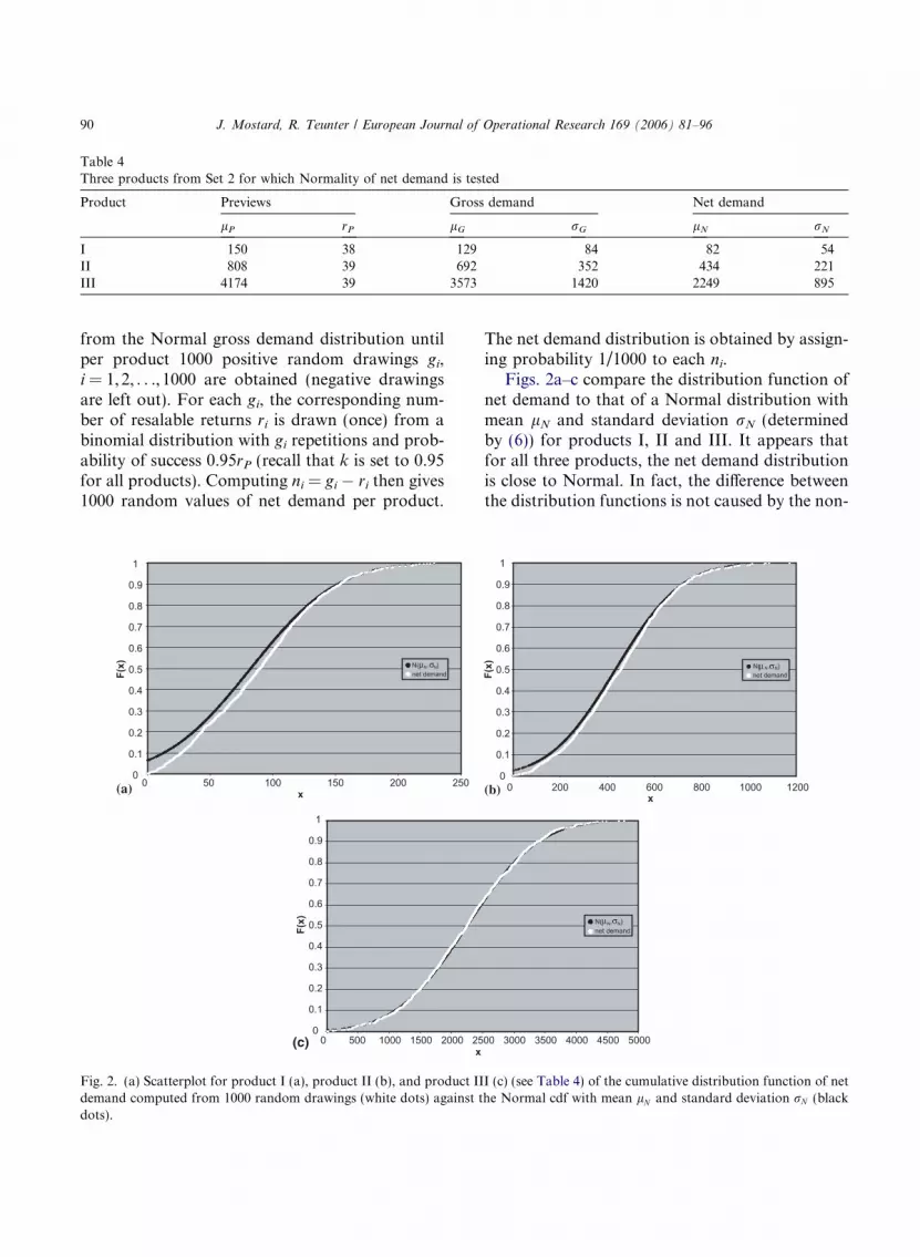
Table 4Three products from Set 2 for which Normality of net demand is tested

Product Previews Gross demand Net demand

lP rP lG rG lN rN

I 150 38 129 84 82 54II 808 39 692 352 434 221III 4174 39 3573 1420 2249 895

90 J. Mostard, R. Teunter / European Journal of Operational Research 169 (2006) 81–96

from the Normal gross demand distribution untilper product 1000 positive random drawings gi,i = 1,2, . . ., 1000 are obtained (negative drawingsare left out). For each gi, the corresponding num-ber of resalable returns ri is drawn (once) from abinomial distribution with gi repetitions and prob-ability of success 0.95rP (recall that k is set to 0.95for all products). Computing ni = gi � ri then gives1000 random values of net demand per product.

0

0.1

0.2

0.3

0.4

0.5

0.6

0.7

0.8

0.9

1

0 500 1000 1500 2000 25x

F(x)

0

0.1

0.2

0.3

0.4

0.5

0.6

0.7

0.8

0.9

1

0 50 100 150 200 250x

F(x) N(µN.σN)

net demand

(c)

(a)

Fig. 2. (a) Scatterplot for product I (a), product II (b), and product IIdemand computed from 1000 random drawings (white dots) against tdots).

The net demand distribution is obtained by assign-ing probability 1/1000 to each ni.

Figs. 2a–c compare the distribution function ofnet demand to that of a Normal distribution withmean lN and standard deviation rN (determinedby (6)) for products I, II and III. It appears thatfor all three products, the net demand distributionis close to Normal. In fact, the difference betweenthe distribution functions is not caused by the non-

00 3000 3500 4000 4500 5000

N( N. N) net demand

0

0.1

0.2

0.3

0.4

0.5

0.6

0.7

0.8

0.9

1

0 200 400 600 800 1000 1200x

F(x) N( N. N)

net demandµ σ

µ σ

(b)

I (c) (see Table 4) of the cumulative distribution function of nethe Normal cdf with mean lN and standard deviation rN (black

J. Mostard, R. Teunter / European Journal of Operational Research 169 (2006) 81–96 91

Normality of net demand if gross demand is Nor-mal. Instead, it results from the non-Normality ofgross demand, since demands cannot be negative.This explains why the difference decreases withlN/rN. Fortunately, that ratio is higher than 1.5for all products that will be considered in the nextsection, justifying the assumption of Normal grossdemand.

7. Computational experiments

Using the data in Set 2, we perform computa-tional experiments to compare the exact optimalorder quantity Q* to the approximate order quan-tity bQ and to the order quantity eQ (resulting fromthe order rule) currently used by the retailer. Thecurrent order quantity is equal to the expectednet demand, i.e.,eQ ¼ lP ð1� rkÞ: ð13ÞRecall from Section 2 that eQ is actually an order-up-to level instead of an order quantity, since thepreview order on which we focus is the secondorder. However, as we argued in that section, thepreview order is the key order and we consider itto be the only order in this study.

Besides a comparison of Q�, bQ, and eQ for allproducts together, we illustrate their differencesfor a selection of nine products from Set 2. The rel-evant cost and demand data are given in Table 5.

These nine products were selected to display theeffect of a product�s profit margin, its expectedgross demand and its expected return probability

Table 5Data for the selected group of nine products from Set 2

Product c p (p � c)/c s r =

1 7.56 35.00 3.63 2.27 0.32 14.02 49.95 2.56 4.21 0.33 16.35 38.85 1.38 4.91 0.34 30.64 89.95 1.94 9.19 0.35 13.66 39.95 1.92 4.10 0.46 13.66 39.95 1.92 4.10 0.47 14.85 49.95 2.36 4.46 0.5

8 17.28 59.95 2.47 5.18 0.4

9 8.75 29.90 2.42 2.63 0.3

Note that k = 0.95 and d = 4.25 for all products.

on the order quantities and on the associated ex-pected profits. Products 1–3 in the table are chosenaccording to decreasing relative profit margin(p � c)/c, products 4–6 according to decreasing ex-pected gross demand lG, and products 7–9 accord-ing to decreasing expected return probability r.Moreover, to isolate the effect of the decreasingparameter, the products are chosen such that allother parameters are approximately constant overevery three products for which one of the afore-mentioned parameters is decreasing.

To display the effect of the shortage cost g

(equal for all products), we use three different val-ues: g = 0, g = 10, and g = 50.

7.1. Results

We first compare the order quantities and ex-pected profits for the nine selected products, andwill then discuss cumulative results for all productsin Set 2. Table 6 displays the results for the selectednine products. Table 7 gives a detailed view of theseparate revenues and costs.

The first main conclusion is that the currentorder quantity eQ is too small, often more than10% smaller than the optimal order quantity Q*.This holds even if the shortage cost g is set to 0,though the differences are larger, of course, forg = 10, 50. The effect on the expected profit issmall (up to 4% decrease) if g = 0, considerable(up to 13% decrease) if g = 10, and can be verylarge (up to 78% decrease) if g = 50.

The result that eQ < Q� even for g = 0 showsthat, by ordering more, the retailer can increase

rP lP lG rG lN rN

7 545 466 251 301 1637 545 466 251 301 1637 545 466 251 301 1639 3451 2954 1208 1860 7610 1253 1072 511 662 3151 478 409 225 250 1383 572 490 262 242 1304 566 484 260 280 1517 599 513 273 331 177

Table 6Results for a selection of nine products from Set 2

Product Order quantity Expected profit

Q* bQ eQ EP(Q*) EPðbQÞ EPðeQÞg = 0

1 450 496 (+10%) 352 (�22%) 5979 5932 (�1%) 5715 (�4%)2 419 459 (+10%) 352 (�16%) 7582 7522 (�1%) 7388 (�3%)3 353 378 (+7%) 352 (�0%) 3864 3842 (�1%) 3864 (�0%)

4 2295 2546 (+11%) 2172 (�5%) 81245 80254 (�1%) 80985 (�0%)5 828 917 (+11%) 773 (�7%) 11296 11164 (�1%) 11242 (�0%)6 323 356 (+10%) 293 (�9%) 4047 4005 (�1%) 4009 (�1%)

7 321 386 (+20%) 282 (�12%) 5133 4951 (�4%) 5054 (�2%)8 385 438 (+14%) 327 (�15%) 8119 7984 (�2%) 7937 (�2%)9 448 490 (+9%) 387 (�14%) 4570 4534 (�1%) 4483 (�2%)

g = 10

1 494 549 (+11%) 352 (�29%) 5791 5719 (�1%) 5055 (�13%)2 456 503 (+10%) 352 (�23%) 7302 7209 (�1%) 6729 (�8%)3 412 450 (+9%) 352 (�15%) 3374 3312 (�2%) 3204 (�5%)

4 2411 2691 (+12%) 2172 (�10%) 79368 78053 (�2%) 78244 (�1%)5 929 1045 (+12%) 773 (�17%) 10561 10304 (�2%) 9976 (�6%)6 367 413 (+13%) 293 (�20%) 3722 3632 (�2%) 3412 (�8%)

7 362 449 (+24%) 282 (�22%) 4805 4451 (�7%) 4363 (�9%)8 418 482 (+15%) 327 (�22%) 7809 7599 (�3%) 7251 (�7%)9 511 565 (+11%) 387 (�24%) 4270 4198 (�2%) 3769 (�12%)

g = 50

1 569 638 (+12%) 352 (�38%) 5454 5328 (�2%) 2419 (�56%)2 527 589 (+12%) 352 (�33%) 6728 6552 (�3%) 4092 (�39%)3 505 562 (+11%) 352 (�30%) 2530 2361 (�7%) 568 (�78%)

4 2687 3031 (+13%) 2172 (�19%) 74687 72453 (�3%) 67283 (�10%)5 1096 1251 (+14%) 773 (�29%) 9265 8735 (�6%) 4912 (�47%)6 441 503 (+14%) 293 (�34%) 3153 2951 (�6%) 1025 (�67%)

7 430 549 (+28%) 282 (�34%) 4231 3544 (�16%) 1598 (�62%)8 484 567 (+17%) 327 (�32%) 7159 6766 (�5%) 4510 (�37%)9 605 678 (+12%) 387 (�36%) 3789 3643 (�4%) 913 (�76%)

The percentual deviations are relative to the optimal order quantity Q* and to the associated optimal profit EP(Q*).

92 J. Mostard, R. Teunter / European Journal of Operational Research 169 (2006) 81–96

profit (excluding loss of goodwill costs) and reducethe number of lost sales at the same time. The poorperformance of eQ determined by (13) can beattributed to its simplicity, and especially to theinability to take into account relevant cost param-eters. Besides not considering the shortage cost g,eQ does not differentiate between highly and lessprofitable products. Clearly, it is better to order

relatively more products with a high profit margin.Products 1–3 in Table 6 illustrate this.

Next, we compare bQ to Q* for the selection ofnine products. It turns out that bQ is always lar-ger than the optimal order quantity, 13% onaverage. Recall that bQ is based on the assump-tions that items can be resold only once and thata fixed percentage of returns is resalable. Recall

Table 7Detailed revenue/cost results for a selection of nine products from Set 2

Product eQ bQ Q*

p s c d g p s c d g p s c d g

g = 0

1 8780 229 �2660 �634 �0 9917 483 �3751 �716 �0 9685 392 �3399 �700 �02 12530 425 �4933 �634 �0 13904 762 �6440 �704 �0 13517 625 �5875 �684 �03 9761 497 �5762 �633 �0 10095 579 �6178 �654 �0 9774 499 �5776 �633 �04 147048 4941 �66563 �4442 �0 155450 7518 �78018 �4696 �0 150378 5727 �70317 �4543 �05 22572 854 �10563 �1621 �0 24144 1283 �12529 �1734 �0 23272 1007 �11312 �1671 �06 8261 352 �3999 �606 �0 8987 536 �4859 �659 �0 8655 435 �4409 �635 �07 9818 383 �4193 �953 �0 11016 739 �5734 �1070 �0 10414 504 �4774 �1011 �08 13882 496 �5655 �786 �0 15503 930 �7571 �878 �0 14904 704 �6645 �844 �09 8279 289 �3384 �700 �0 9100 487 �4283 �769 �0 8834 400 �3917 �747 �0

g = 10

1 8780 229 �2660 �634 �659 10073 593 �4150 �728 �70 9906 478 �3732 �716 �1462 12530 425 �4933 �634 �659 14192 924 �7059 �718 �129 13874 749 �6388 �702 �2303 9761 497 �5762 �633 �659 10768 850 �7362 �698 �247 10458 700 �6733 �678 �3734 147048 4941 �66563 �4442 �2740 157466 8644 �82459 �4757 �842 152992 6525 �73871 �4622 �16575 22572 854 �10563 �1621 �1266 24926 1728 �14281 �1790 �279 24240 1323 �12695 �1741 �5666 8261 352 �3999 �606 �597 9357 732 �5637 �686 �134 9083 575 �5020 �666 �2507 9818 383 �4193 �953 �691 11286 997 �6674 �1096 �62 10843 648 �5382 �1053 �2528 13882 496 �5655 �786 �685 15800 1132 �8329 �894 �110 15309 841 �7217 �867 �2579 8279 289 �3384 �700 �714 9397 661 �4947 �795 �118 9203 533 �4467 �778 �221

g = 50

1 8780 229 �2660 �634 �3296 10188 788 �4824 �736 �88 10112 636 �4303 �730 �2602 12530 425 �4933 �634 �3296 14473 1258 �8252 �733 �195 14299 1014 �7390 �724 �4713 9761 497 �5762 �633 �3296 11226 1338 �9181 �727 �295 11057 1080 �8250 �716 �6404 147048 4941 �66563 �4442 �13702 160307 11476 �92868 �4843 �1620 157421 8615 �82345 �4755 �42495 22572 854 �10563 �1621 �6330 25444 2518 �17090 �1827 �309 25118 1916 �14973 �1804 �9926 8261 352 �3999 �606 �2985 9602 1078 �6877 �704 �149 9467 835 �6021 �694 �4357 9818 383 �4193 �953 �3456 11411 1428 �8146 �1108 �41 11226 914 �6380 �1090 �4388 13882 496 �5655 �786 �3427 16070 1549 �9801 �910 �144 15808 1139 �8355 �895 �5379 8279 289 �3384 �700 �3571 9569 941 �5929 �809 �128 9484 757 �5295 �802 �355

Separate returns and costs are shown for all three order quantities, eQ, bQ and Q*.

J.Mosta

rd,R.Teunter

/EuropeanJournalofOpera

tionalResea

rch169(2006)81–96

93

Table 8Cumulative results for all products in Set 2

g Expected profit Lost sales percentage

EP(Q*) EPðbQÞ EPðeQÞ LS(Q*) LSðbQÞ LSðeQÞ0 3190340 3156470 (�1%) 3127520 (�2%) 8% 5% 13%10 3058070 3004680 (�2%) 2850970 (�5%) 5% 3% 13%50 2797180 2696130 (�4%) 1744770 (�38%) 2% 1% 13%

The percentual deviations for the expected profits are relative to EP(Q*). The lost sales percentage LS(Q) is the fraction of grossdemands that are lost (one minus the �fill rate�).

94 J. Mostard, R. Teunter / European Journal of Operational Research 169 (2006) 81–96

further that the first assumption leads to an up-ward bias of the order quantity whereas the sec-ond one leads to a downward bias. Apparently,the effect of the �single resale� assumption is dom-inant. This also explains why the difference be-tween bQ and Q* is especially large if the returnrate is high, since a higher return rate increasesthe probability that products are resold morethan once.

Table 6 further shows that the difference be-tween bQ and Q* is almost constant in g. The differ-ence between the associated expected profits,however, increases considerably in g. The explana-tion for this result is that, as for the traditionalnewsvendor problem without returns, the expectedprofit curve EP(Q) is steeper on the right hand sidefor larger values of g.

We end with a comparison of Q*, bQ, and eQ forall products in Set 2 together. Table 8 gives thecumulative numbers for the expected profits andthe expected lost sales percentages. We remarkthat a comparison of the realized profits and therealized lost sales percentages, calculated usingthe realized demand data in Set 2, produced simi-lar results.

Table 8 shows that the percentage of lost salesassociated with bQ is relatively much smaller thanthe percentage of lost sales associated with theoptimal order quantity Q*. This is because bQ isoften much larger than Q* (see the previous discus-sion of the results for the selection of nine prod-ucts). The overall effect on the profit is small,however, since the profit curve is rather flat aroundthe optimum, especially for small values of g.Ordering bQ instead of Q* leads to a profit reduc-tion of 1% for g = 0, 2% for g = 10, and 4% forg = 50.

The overall performance of the current orderquantity is very poor. The associated lost salespercentage is 13%, whereas the optimal lost salespercentage is at most 5% (less if g > 0). Using eQinstead of Q* leads to a profit reduction of2% for g = 0, 5% for g = 10, and 38% for g =50.

8. Conclusion

We derived a simple closed-form formula thatdetermines the optimal order quantity Q* for a sin-gle period inventory (newsboy) problem with re-turns. Using real data from a large catalogue/internet mail order company, Q* was comparedto an approximation bQ proposed in a previousstudy and to the order quantity eQ currently usedby the company. It turned out that bQ differs morethan 10% from Q* in most cases. The associatedprofit reduction is generally smaller than 5%, butmore than 10% in cases with a high return rateand a high shortage cost. The company�s orderquantity eQ is far from optimal. It is much smaller(often more than 20%) than Q*. Even if the short-age cost is ignored, the company could increaseprofit by ordering more (while reducing the num-ber of lost sales at the same time).

Due to a lack of data (only forecasts and real-izations for multiple items for a single periodare available), we had to develop a procedurefor estimating the variance of demand. The simpleprocedure that we developed suffices for the pur-poses of this paper. It would be interesting,though, to do further statistical research into thisforecasting problem and compare different proce-dures.

J. Mostard, R. Teunter / European Journal of Operational Research 169 (2006) 81–96 95

In this paper, we focused on the second of themail order company�s three order moments, thepreview. It would be interesting to extend ourmodel with especially an additional in-seasonemergency replenishment option. Such a modelcan provide useful insights into the simultaneousdetermination of the two optimal order quantitiesand into the profitability of the additional replen-ishment option. For the newsboy problem withoutreturns, it has been shown (see e.g. Khouja [2])that an emergency order can lead to a substantialincrease in profit. However, the typical assump-tions of negligible fixed emergency ordering costand negligible emergency lead time do not holdin our case study. Therefore, including an emer-gency option is certainly not straightforward. Be-sides the effect on the regular order, the timingand size of the emergency order need to be ana-lyzed.

Acknowledgements

The authors thank the two anonymous refe-rees for their helpful comments. The research ofDr. Ruud H. Teunter has been made possible bya fellowship of the Royal Netherlands Academyof Arts and Sciences.

The research presented in this paper is part ofthe research on re-use in the context of the EUsponsored TMR project REVersed LOGistics(ERB 4061 PL 97-5650) in which the ErasmusUniversity Rotterdam (NL), the Otto-von-Guer-icke Universitat Magdeburg (D), the EindhovenUniversity of Technology (NL), INSEAD (F),the Aristoteles University of Thessaloniki (GR),and the University of Piraeus (GR) take part.

Appendix A. A mean and variance of net demand

Using

E½K� ¼X1n¼0

Pr½G ¼ n�E½KjG ¼ n�

¼X1n¼0

Pr½G ¼ n�rkn ¼ rkE½G�;

E½K2� ¼X1n¼0

Pr½G¼ n�E½K2jG¼ n�

¼X1n¼0

Pr½G¼ n�ðV ½KjG¼ n� þ ðE½KjG¼ n�Þ2Þ

¼X1n¼0

Pr½G¼ n�ðnrkð1� rkÞ þ ðrknÞ2Þ

¼ rkð1� rkÞE½G� þ ðrkÞ2E½G2�¼ rkð1� rkÞE½G� þ ðrkÞ2ðV ½G� þ ðE½G�Þ2Þ¼ rkð1� rkÞE½G� þ ðrkÞ2V ½G� þ ðrkÞ2ðE½G�Þ2Þ;

and

E½GK� ¼X1n¼0

Pr½G ¼ n�E½GKjG ¼ n�

¼X1n¼0

Pr½G ¼ n�nE½KjG ¼ n�

¼X1n¼0

Pr½G ¼ n�nðrknÞ ¼ rkE½G2�

¼ rkðV ½G� þ ðE½G�Þ2Þ ¼ rkV ½G� þ rkðE½G�Þ2;we get

lN ¼ E½N � ¼ E½G� K� ¼ E½G� � E½K�¼ E½G� � rkE½G� ¼ ð1� rkÞE½G� ¼ ð1� rkÞlG

and

ðrNÞ2 ¼ V ½N � ¼ V ½G� K�¼ V ½G� þ V ½K� � 2Cov½G;K�¼ V ½G� þ E½K2� � ðE½K�Þ2

� 2ðE½GK� � E½G�E½K�Þ¼ V ½G� þ rkð1� rkÞE½G� þ ðrkÞ2V ½G�þ ðrkÞ2ðE½G�Þ2 � ðrkÞ2ðE½G�Þ2

� 2ðrkV ½G� þ rkðE½G�Þ2 � E½G�rkE½G�Þ¼ ð1þ ðrkÞ2 � 2rkÞV ½G� þ rkð1� rkÞE½G�¼ ð1� rkÞ2V ½G� þ rkð1� rkÞE½G�¼ ð1� rkÞ2ðrGÞ2 þ rkð1� rkÞlG:

References

[1] R.M. Hill, Applying Bayesian methodology with a uniformprior to the single period inventory model, EuropeanJournal of Operational Research 98 (3) (1997) 555–562.

96 J. Mostard, R. Teunter / European Journal of Operational Research 169 (2006) 81–96

[2] M. Khouja, A note on the newsboy problem with anemergency supply option, Journal of the OperationalResearch Society 47 (1996) 1530–1534.

[3] M. Khouja, The single-period (news-vendor) problem:Literature review and suggestions for future research,Omega The International Journal of Management Science27 (1999) 537–553.

[4] M. Kodama, Probabilistic single period inventorymodel with partial returns and additional orders, Com-puters and Industrial Engineering 29 (1–4) (1995) 455–459.

[5] C.H. Lee, Coordinated stocking, clearance sales and returnpolicies for a supply chain, European Journal of Opera-tional Research 131 (3) (2000) 1–12.

[6] W. Shih, A note on Bayesian approach to newsboyinventory problem, Decision Sciences 4 (2001) 184–194.

[7] E.A. Silver, D.F. Pyke, R. Peterson, Inventory Managementand Production Planning and Scheduling, third ed., JohnWiley & Sons, New York, 1998.

[8] D. Vlachos, R. Dekker, Return handling options and orderquantities for single period products, European Journal ofOperational Research 151 (1) (2003) 38–52.