The NAFTA tide: Lifting the larger and better boats

IZA DP No. 3207

The NAFTA Tide: Lifting the Larger and Better Boats

Angel Calderon-MadridAlexandru Voicu

DI

SC

US

SI

ON

PA

PE

R S

ER

IE

S

Forschungsinstitutzur Zukunft der ArbeitInstitute for the Studyof Labor

December 2007

The NAFTA Tide:

Lifting the Larger and Better Boats

Angel Calderon-Madrid El Colegio de México

Alexandru Voicu

CUNY, College of Staten Island and IZA

Discussion Paper No. 3207 December 2007

IZA

P.O. Box 7240 53072 Bonn

Germany

Phone: +49-228-3894-0 Fax: +49-228-3894-180

E-mail: [email protected]

This paper can be downloaded without charge at: http://ssrn.com/abstract=1081643

An index to IZA Discussion Papers is located at:

http://www.iza.org/publications/dps/

Any opinions expressed here are those of the author(s) and not those of the institute. Research disseminated by IZA may include views on policy, but the institute itself takes no institutional policy positions. The Institute for the Study of Labor (IZA) in Bonn is a local and virtual international research center and a place of communication between science, politics and business. IZA is an independent nonprofit company supported by Deutsche Post World Net. The center is associated with the University of Bonn and offers a stimulating research environment through its research networks, research support, and visitors and doctoral programs. IZA engages in (i) original and internationally competitive research in all fields of labor economics, (ii) development of policy concepts, and (iii) dissemination of research results and concepts to the interested public. IZA Discussion Papers often represent preliminary work and are circulated to encourage discussion. Citation of such a paper should account for its provisional character. A revised version may be available directly from the author.

IZA Discussion Paper No. 3207 December 2007

ABSTRACT

The NAFTA Tide: Lifting the Larger and Better Boats*

We use panel data on Mexican manufacturing plants to study the connection between plants’ responses to changes in the economic environment and their contributions to aggregate productivity growth in the period following the implementation of the North American Trade Agreement (NAFTA). In all industries, an overwhelming share of aggregate productivity growth is accounted for by a small number of plants which were larger and more productive before the implementation of NAFTA and expanded and became more productive following the implementation of NAFTA. Plants that exported before NAFTA and export continuously through 2000 and some of the new exporters are more likely to be among the top-performing plants. Exporting activity and performance of plants with similar exporting experience, however, display remarkable heterogeneity. This heterogeneity implies that trade liberalization provided growth opportunity to larger and more productive plants irrespective of their export status and provides an explanation for the lackluster average productivity performance of exporting plants. JEL Classification: C13, D24, F13, O47, O54 Keywords: NAFTA, trade liberalization, productivity, heterogeneity of plant-level performance Corresponding author: Alexandru Voicu CUNY, College of Staten Island PEP Department 2800 Victory Blvd. Staten Island, NY 10314 USA E-mail: [email protected]

* The authors are grateful to John Haltiwanger, Adriana Kugler, Eric Verhoogen, the participants of the conference "Job Reallocation, Productivity Dynamics and Trade Liberalization,” (Bogota, 2005), the participants of the Bank of Mexico Direccion General de Investigacion Economica seminar (July 2005), and Michael Lahr for their many comments and suggestions. The help from Abigael Duran of the Mexican National Institute of Statistics, INEGI, in Aguascalientes, Mexico, were very useful in the elaboration of this paper. We are grateful to him, to Alex Cano, and to the staff of INEGI for making this research possible. The conclusions expressed here and remaining errors are exclusive responsibility of the authors.

1 Introduction

The relationship between plants’ exporting activity and their productivity performance has been the

focus of recent empirical and theoretical trade literature.3 The existence of plant-level productivity

gains from exporting is important from a policy perspective.4 Post-entry productivity gains —

involvement in the export markets may raise returns to innovation, alow plants to exploit economies

of scale, or force them to reduce X-inefficiency — as well as pre-entry productivity gains, if plants

have to become more productive in order to enter the export markets, justify trade promotion and

trade liberalization policies. Without productivity gains from exporting, trade promotion policies

lead to plants self-selecting into subsidies and, potentially, incurring the considerable downside risks

of exporting.

Previous studies of trade liberalization episodes and periods with rapidly falling trade costs5

reveal that reductions in the costs of trade lead to higher aggregate, industry-level productivity

— the efficiency with which industry’s output is produced — but little if any of this growth comes

from plant-level efficiency gains related to exporting activity. Evidence with respect to the relation-

ship between exporting and post-entry productivity growth is weak: future performance of current

exporters is at best as good as that of plants that do not export. Instead, the link between the

reduction in the costs of trade and aggregate productivity growth lies in the correlation between

plants’ characteristics and plants’ responses to trade liberalization.6 In industries with heteroge-

3Tybout (2003) and Greenway and Kneller (2007) provide reviews of the literature on the relationship betweenplant performance, exporting, and foreign investment.

4Bernard and Jensen (1999)5Pavcnik (2002), Tybout and Westbrook (1995) and Lopez-Cordova (2002) study trade liberalization episodes in

Chile and Mexico; Bernard, Jensen, and Schott (2006) use data on US manufacturing plants that cover the periodbetween 1982 and 1997 during which tariffs declined by more than 25 percent in a majority of industries.

6Melitz (2004), Helpman, Melitz, and Yeaple (2004), Bernard, Eaton, Jensen, and Kortum (2003) propose theoret-ical models of imperfectly competitive industries with heterogeneous firms in which the link between the reduction inthe costs of trade and aggregate productivity growth lies in the correlation between plants’ productivity and plants’responses to trade liberalization.

2

neous plants and fixed costs of exporting, more productive plants become exporters. Reductions

in trade costs force least-productive firms to exit the market, increase the number of exporters —

more productive firms become exporters — enhance sales by existing exporters, and reduce domestic

market share of surviving firms. This trade-induced reallocation of market share from less to more

productive plants leads to aggregate, industry-level productivity growth in the absence of plant-level

productivity gains from exporting.

Plants that undertake exporting activities, however, meet with various degrees of success.7

There is significant, simultaneous entry into and exit from the export market and changes in export

status represent important junctures in plants’ lives. For a short period following entry into the

foreign markets, exporting plants grow, on average, faster than plants that do not export. Over

time, some of them will fail and exit the export market. The performance of plants that exit is,

on average, weaker than that of plants that never export, while those that continue their export

operations grow faster than plants that never export. Over longer periods of time, due to this

heterogeneity of exporting activity, the performance of plants that enter the export market at any

given point in time is not, on average, better than that of plants that never export. These results

suggest that, following trade liberalization, plants’ contributions to aggregate productivity growth

are far more heterogeneous than predicted by the theoretical models. They also leave open the

possibility that, while, on average, exporting plants do not have better productivity performance

than non-exporting plants, for a subset of plants a reduction in the costs of trade may lead to both

output and productivity growth.

In this paper we use data on Mexican manufacturing plants to study the connection between

plants’ responses to changes in the economic environment and their contributions to aggregate pro-

7Bernard and Jensen (1999, 2004)

3

ductivity growth in the period following the implementation of the North American Trade Agree-

ment (NAFTA). Our data, an unbalanced panel of non-maquiladora plants8 from eight two-digit

industries, cover the period between 1993 and 2000, a period that, in addition to the introduction

of NAFTA in 1994, encompassed a severe macroeconomic crisis in 1995 and the temporary deval-

uation of the Mexican peso. We document the intra-industry heterogeneity of plants’ responses to

the changes in the economic environment paying special attention to changes in the export status.

We estimate plant-level total factor productivity and use principal component analysis to study the

intra-industry variation in the joint productivity and output performance, the determinants of the

magnitude and nature of plants’ contributions to aggregate productivity. Finally, using the results

of the principal component analysis we analyze the contributions to aggregate productivity growth

of plants with different types of responses to the changes in the economic environment as well as

the heterogeneity of the contributions of firms with similar responses.

We find strong, export-driven, aggregate output and productivity growth in the Mexican man-

ufacturing sector between 1993 and 2000. Exporting and plant-level performance are connected.

In all industries, an overwhelming share of aggregate productivity growth is accounted for by a

small number of plants (roughly 70 percent of percent of the aggregate productivity growth is con-

centrated in 10 percent of the plants). These plants were much larger and more productive than

average before the implementation of NAFTA, and they expanded and became more productive

following the implementation of NAFTA. Plants that exported before NAFTA and export contin-

uously through 2000 and some new entrants have significantly higher probability of being in the

top-performing group. Exporting activity and performance of plants with similar exporting experi-

ence, however, display remarkable heterogeneity. This heterogeneity implies, on the one hand, that

8A maquiladora or maquila is a factory that imports materials and equipment on a duty-free and tariff-free basisfor assembly or manufacturing and then re-exports the assembled product, usually back to the originating country.

4

trade liberalization provided growth opportunity to larger and more productive plants regardless of

their export status. On the other hand, it generates aggregate patterns that differ from the predic-

tions of the theoretical models. While plants that exported in 1993, especially those that continued

to export until 2000, were larger to begin with and grew more than those that did not export, we

find no evidence that exporting plants, even long-term exporters were, on average, more productive

than non-exporters and, therefore, their expansion could not lead to aggregate productivity growth.

The remainder of the paper is structured as follows. Section 2 contains background information

on NAFTA and a description of the data set used in this paper. In section 3 we analyze aggregate

industry-level performance between 1993 and 2000 and document the heterogeneity of plants’ re-

sponses to the changes in the economic environment. The estimation of industry-level production

functions is presented in section 4, together with an analysis of aggregate industry-level productiv-

ity. In section 5 we study the connection between plant-level responses to changes in the economic

environment and plant-level contributions to aggregate productivity growth. We conclude with a

summary of the main findings and a discussion of their implications.

2 Background and Data

In mid 1980s, as part of its accession to GATT, Mexico substantially reduced and rationalized

tariffs and undertaken privatization, deregulation, and other major economic reforms. The North

American Free Trade Agreement (NAFTA), signed in December 1992 and implemented in January

1994, was aimed at creating an integrated market in North America. NAFTA included provisions

for progressive elimination of tariff and non-tariff barriers to goods trade, improvement of access for

services trade, creation of a stable and transparent legal framework for foreign investors, stronger

protection of intellectual property rights, and creation of an effective dispute settlement mechanism;

5

NAFTA removed or phased out measures designed to discourage the free flow of capital between

Canada, Mexico, and the US. Previous literature shows that NAFTA had an important effect on

Mexico’s economy: the volume of trade grew substantially, the composition of trade changed, FDI

flows increased considerably, and total factor productivity grew faster in the manufacturing sector.9

In this paper we use an unbalanced panel data set of non-maquiladora manufacturing plants from

eight two-digit industries: food processing, textiles, wood, paper, chemicals, glass, basic metals, and

machinery. The plants were followed for eight years, between 1993 and 2000, which allows us to

observe them both before and after the implementation of NAFTA. The data set was constructed

using information from two main sources, Annual Industrial Survey (AIS) and Industrial Census

(IC). AIS is a survey of manufacturing establishments that uses a non-probabilistic sample (the

sample selection startegy is descibed in Appendix A.1). The sample was selected using IC 1993 as

universe and included predominantly large and medium-scale plants, but also a significant number

of small plants from 205 six-digit industries. Selected plants account for at least 80 percent of the

total value of production of their respective industry. Establishments that operate under the special

maquiladora regime and petrochemical and oil-refining plants, which are state-owned monopoly, are

excluded from the sample. AIS provides information on a wide range of variables: investment and

sales of capital, rent on buildings paid by the plant, value added, skilled and unskilled labor,

electricity usage, total sales, domestic sales, and exports, and use of imported intermediary inputs.

IC takes place every five years and in this paper we use information from the 1993 and 1998 surveys.

IC contains information on replacement value and depreciation for six categories of capital stock:

machinery, buildings, land, transportation equipment, computing and peripheral equipment, and

9Lederman, Maloney, and Serven (2003) use sectoral data and find faster convergence rates during NAFTA. Usingfirm-level evidence, Lopez-Cordova (2002) finds an increase in TFP in NAFTA years due to preferential access tothe US market and import competition, but not from the use of imported inputs. Schiff and Wang (2003) use sectordata and find that on the contrary use of imported intermediary inputs is responsible for TFP growth.

6

furniture and office equipment. Firms are asked to consider reevaluations due to exchange rate

variations and to account for physical deterioration and obsolescence.

We use information from the two sources to construct plant-level time series for a set of plant

characteristics and measures of performance. We combine data on replacement value of the capital

stock from the IC with data from AIS on investment and sales of capital, and rent on buildings

paid by the plant to impute the replacement value of capital stock for each firm for all the years

(a detailed description of the imputation procedure is given in the Appendix A.2). The imputed

capital stock, value added, skilled and unskilled labor, and electricity usage are used to estimate

the industry-specific production functions and construct plant-level total factor productivity series.

Total, domestic, and export sales, shares of imported inputs, capital intensity, share of skilled

labor, and foreign direct investment are used in the subsequent analysis. Value added and sales

were deflated using a price index generated by INEGI for 205 sectors. We exclude from the analysis

plants with missing information on the variables of interest for any of years they were present in

the sample. Among plants that exit the AIS sample between 1993 and 2000, we use in the analysis

only those that closed down (shut down, bankrupt, and liquidated). The resulting sample contains

4,127 plants and 30,534 plant-year observations, in eight manufacturing industries.

Like all other studies measuring the effect of NAFTA on the performance of Mexican plants,

ours has two limitations. Our data set covers a period that, in addition to the implementation

of NAFTA, encompasses a period of exchange rate devaluation, following the collapse of peso

in December 1994, and a severe macroeconomic crisis. Effects of the unilateral policy of trade

liberalization undertaken after 1985 were likely to be present after 1994 and, in turn, some NAFTA

provisions will not be fully implemented until 2009. NAFTA itself was a nexus of provisions —

removal of tariff and non-tariff barriers to the goods trade, removal of barriers to service trade,

7

creation of a stable and transparent legal framework for foreign investors, stronger protection of

intellectual property rights. As a result, it is difficult to trace the effects of individual components of

NAFTA, of NAFTA itself, or of the exchange rate devaluation on the performance of manufacturing

plants. In this paper, we analyze plants’ responses to the changes in the economic environment,

specifically exits from the market and changes in the export status, and the relationship between

these responses and plant-level performance. Second, initial conditions were asymmetric. Even

after the unilateral trade liberalization, Mexico retained higher tariff and non-tariff barriers than

both US and Canada. Therefore, it is expected that transition costs will be relatively higher for

Mexico. By studying performance during a relatively short period after implementation, results are

likely to be affected by the short-run transition costs.

3 Aggregate industry-level performance

We begin our empirical analysis with an assessment of the aggregate, industry-level performance

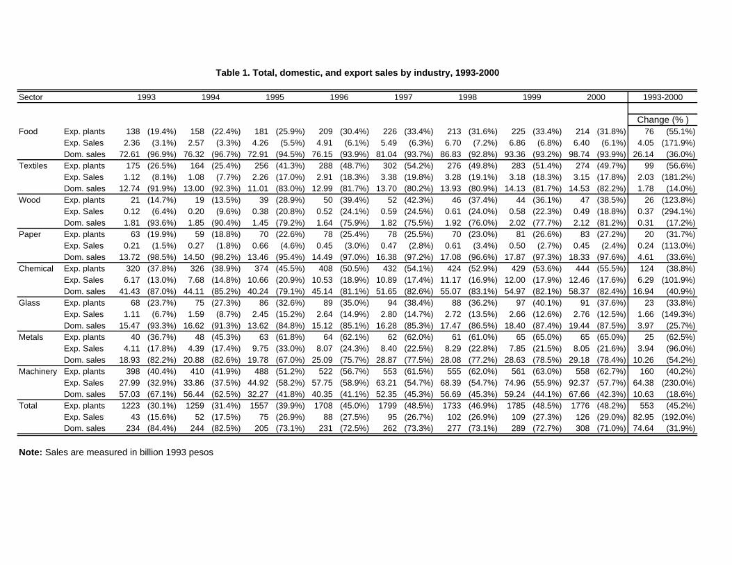
of the Mexican manufacturing sector following the introduction of NAFTA. Table 1 presents the

number of exporting plants, domestic sales, and export sales, in our sample, between 1993 and

2000. The data show tremendous overall growth in the Mexican manufacturing sector between

1993 and 2000, and suggest that stronger exporting activity following the introduction of NAFTA

accounts for a large share of the aggregate growth. Overall, total sales increased by 56 percent and

roughly half of this growth is accounted for by the rise in exports: the number of exporting plants

increased by 45 percent, export sales nearly doubled, while domestic sales increased by 32 percent.

Aggregate performance varies widely over time and across industries. The highest rates of growth

in exports prevail between 1995 and 1997, when the effects of NAFTA and those of the exchange

rate devaluation overlap. On the other hand, the domestic crisis of 1995 had a strong negative effect

8

on domestic sales in all industries. The machinery industry accounts for two thirds of the total

exports made between 1993 and 2000 and for more than 75 percent of the growth in exports, while

the three industries with the largest exports — machinery, chemical, and primary metals — account

for almost 90 percent of both total export sales and growth in exports. The three industries with

the largest output — food, chemical, and machinery — account for 75 percent of the total sales made

between 1993 and 2000 and for 80 percent of the increase in sales.

Aggregate industry-level growth described in table 1 was generated by plant responses to changes

in the economic environment that display a high degree of within-industry heterogeneity. Table 2

shows, by year, the percentage of plants in the sample that exit the market, the percentage of

plants selling exclusively on the domestic market that begin exporting, the percentage exporting

plants that stop exporting, and the percentages of exporting plants that increase and decrease their

export sales by at least 25 percent. In all industries significant percentages of plants exit the market.

Rates of exit are largest in 1995, the year of the domestic crisis. Between 1993 and 2000, textiles,

wood, and glass industries lost roughly 15 percent of the plants, basic metals and machinery lost

9 percent, and the remaining industries lost around 6 percent of their plants. In all industries,

exporting plants were much less likely to exit the market.

The number of exporting plants and export sales increased dramatically, but changes in the

exporting status display heterogeneity both at the extensive margin and at the intensive margin.

At all times and in all industries, there are both plants that enter the export market and, per-

haps more surprisingly given the period when the favorable effects of NAFTA and exchange rate

liberalization overlap, plants that exit the export market. All industries show the same temporal

pattern: relatively larger percentages of plants start exporting and relatively smaller percentages

stop exporting between 1993 and 1997 when the introduction of NAFTA and the exchange rate

9

devaluation improved exporting conditions. The percentage of plants that start exporting in 1994-

1995, the first year of NAFTA and the period when most plants initiated export operations, ranges

from 5-7 percent in food, paper, and glass to 9-10 percent in chemical and machinery, to 15-18

percent in textiles and wood products. In 1997, when exchange rate rose, the percentage of plants

that start exporting was lowest and the percentage of plants that stop exporting was largest in all

industries.

Among exporters, there are, at all times, both plants that significantly lower their export value

and plants that significantly increase their export levels. In all sectors, the shares of plants increasing

their exports are larger in the years when the favorable effects of NAFTA and the low exchange

rate overlap. The fraction of plants increasing their export values by at least 25 percent between

1994 and 1995 ranges between 60 percent in chemical and machinery industries and 82 percent in

wood products. The share of plants reducing exports increased after the exchange rate returned to

normal levels. Between 1999 and 2000 the fraction of plants reducing their exports by more than

25 percent ranges between 23 percent in machinery and 40 percent in wood products. In the last

years of the panel the share of plants decreasing their exports was generally larger than the share

of plants increasing their exports. Differences across sectors are largest in 1994-1995, when textiles,

wood, and basic metals had the largest shares of plants increasing their exports.

4 Total factor productivity

Two problems must be addressed in estimating production functions with panel data sets. First,

the correlation between input levels and unobserved productivity shocks induces simultaneity bias

in the OLS estimation. Second, plants with low realizations of productivity exit the market. If

plants with larger capital stock are more likely to survive negative realizations of productivity

10

shocks, the OLS estimator of the capital coefficient will be biased. Several ways of dealing with

these problems have been discussed in the literature. Olley and Pakes (1996) proposed a technique

that allows corrections for both simultaneity bias and the selection bias introduced by non-random

exits. A plant’s investment function is modeled as a function of the capital stock capital and the

productivity level unobserved by the econometrician. Under certain conditions, the investment

function can be inverted, thus providing an instrument for the unobserved productivity component.

The selection bias is corrected by formally modeling plants survival decisions and incorporating

them into the estimation. Levinsohn and Petrin (2003) have proposed an approach to correct for

the simultaneity bias that requires less-strict assumptions than those of Olley and Pakes (1996).

They argue that investment responds only to the non-forecastable component of the productivity

shocks and, therefore, the investment function does not perform well if the productivity term has

both a serially correlated component and an idiosyncratic component. Instead, firm’s intermediate

input demand is used to obtain an instrument for the unobserved productivity shock. A number

of recent papers (e.g. Pavcnik, 2002) have used this idea and employed a modified version of the

Olley and Pakes (1996) approach in which the investment function was replaced by the intermediate

input demand. Electricity provides the best instrument since few firms produce it and it cannot

be stored. In this paper we use this later approach. The estimation procedure is described in the

Appendix A.3.

Table 3 shows the estimation results using the two-step semiparametric method that accounts

for the simultaneity and selection biases and, as a comparison benchmark, the results of standard,

fixed-effects OLS estimation. We assume the production function of plant i at time t has a Cobb-

Douglass form:

yit = α+ βslsit + βul

uit + βkkit + ωit + εit

11

where yit is log value added, lsit is log of skilled labor, luit is log of unskilled labor, kit is log of

plant’s capital stock, ωit is the level of plant specific productivity, and εit is white noise. Produc-

tion functions are estimated separately for the eight two-digit SIC manufacturing industries. The

semiparametric estimation yields higher coefficients for capital and skilled labor and lower coeffi-

cients for unskilled labor. This finding is consistent with the presence of simultaneity bias: the use

of easily adjustable factors, like unskilled labor, is positively correlated with productivity shocks,

inducing upward bias of fixed effect estimates. The reverse is true for factors which are slow to

adjust like skilled labor. Higher capital coefficients are consistent with the fact that large firms have

a better chance to survive adverse productivity shocks. These results underscore the importance of

controlling for both selection bias and simultaneity bias in the estimation of production functions.

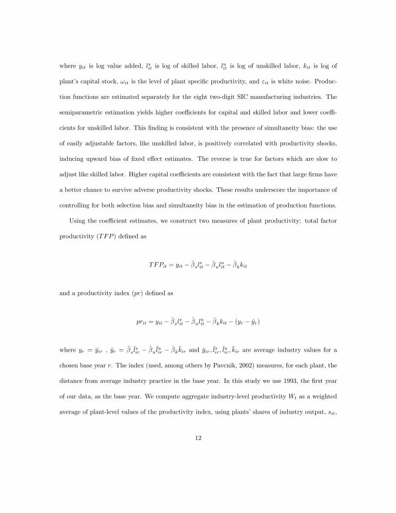
Using the coefficient estimates, we construct two measures of plant productivity: total factor

productivity (TFP ) defined as

TFPit = yit − βslsit − βul

uit − βkkit

and a productivity index (pr) defined as

prit = yit − βslsit − βul

uit − βkkit − (yr − yr)

where yr = yir , yr = βs lsir − βul

uir − βkkir and yir, l

sir, l

uir, kir are average industry values for a

chosen base year r. The index (used, among others by Pavcnik, 2002) measures, for each plant, the

distance from average industry practice in the base year. In this study we use 1993, the first year

of our data, as the base year. We compute aggregate industry-level productivity Wt as a weighted

average of plant-level values of the productivity index, using plants’ shares of industry output, sit,

12

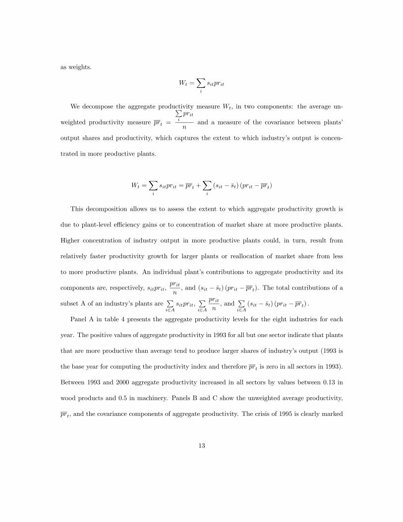
as weights.

Wt =Xi

sitprit

We decompose the aggregate productivity measure Wt, in two components: the average un-

weighted productivity measure prt =

Piprit

nand a measure of the covariance between plants’

output shares and productivity, which captures the extent to which industry’s output is concen-

trated in more productive plants.

Wt =Xi

sitprit = prt +Xi

(sit − st) (prit − prt)

This decomposition allows us to assess the extent to which aggregate productivity growth is

due to plant-level efficiency gains or to concentration of market share at more productive plants.

Higher concentration of industry output in more productive plants could, in turn, result from

relatively faster productivity growth for larger plants or reallocation of market share from less

to more productive plants. An individual plant’s contributions to aggregate productivity and its

components are, respectively, sitprit,pritn

, and (sit − st) (prit − prt). The total contributions of a

subset A of an industry’s plants arePi∈A

sitprit,Pi∈A

pritn

, andPi∈A

(sit − st) (prit − prt) .

Panel A in table 4 presents the aggregate productivity levels for the eight industries for each

year. The positive values of aggregate productivity in 1993 for all but one sector indicate that plants

that are more productive than average tend to produce larger shares of industry’s output (1993 is

the base year for computing the productivity index and therefore prt is zero in all sectors in 1993).

Between 1993 and 2000 aggregate productivity increased in all sectors by values between 0.13 in

wood products and 0.5 in machinery. Panels B and C show the unweighted average productivity,

prt, and the covariance components of aggregate productivity. The crisis of 1995 is clearly marked

13

by sharp drops in prt in all sectors. After 1995, prt raises in most sectors, but over the entire

period increases in only five out of the eight sectors and gains are modest in most sectors. In

textiles, wood products, chemical industry prt declined between 1993 and 2000, in food products

and machinery show modest increases in productivity (around 7%), while paper products, glass,

and primary metals show increases of 15-30 percent in their average productivity.

In all sectors, the covariance component represents the largest share of aggregate productivity,

which means that industry output tends to be strongly concentrated in most productive plants.

Further concentration of industry’s output through reallocation of market share from less productive

to more productive firms is the dominant mechanism for industry productivity gains — with the

exception of basic metals, the growth of covariance component between 1993 and 2000 far exceeds

the growth of the unweighted productivity component for all industries.

5 Responses to changes in the economic environment and

contributions to aggregate productivity growth

The aggregate productivity growth and the relative importance of the covariance component are

common findings in studies of trade liberalization episodes or periods of declining trade costs.

Previous literature shows that the basis of the trade-induced aggregate productivity growth is the

correlation between plants’ productivity and plants’ output performance. Among plants selling

exclusively on the domestic market before trade liberalization, the least productive contract or exit

the market and the more productive expand by entering export market, while plants that exported

before trade liberalization increase their export sales. Exit of the least productive plants raises

the unweighted component of aggregate productivity, but to the extent to which they produce

14

relatively smaller shares of output, it reduces the covariance component, and therefore the overall

effect on aggregate productivity could be either positive or negative. Among the surviving plants,

the reallocation of output from less to more productive leads to an increase in the covariance

component and therefore industry productivity growth.

The heterogeneity of plants’ exporting performance — the simultaneous entry into and exit from

the export market and the large changes in the export sales of continuing exporters — suggests,

however, that the magnitude of the contributions to aggregate productivity growth may differ

significantly among plants that take advantage of NAFTA to enter export markets and among

plants that exported before the introduction of NAFTA. It also leaves open the possibility that the

nature of these contributions is different from that suggested by previous literature, namely gains

in market share by most productive plants that start or intensify exports, and includes plant-level

productivity gains by a subset of exporting plants.

In this section we analyze the contributions to the aggregate productivity of plants with different

types of responses to the changes the economic environment. First, we study plants that exit

the market between 1993 and 2000. Second, for plants in the balanced panel, we use principal

component analysis to study the intra-industry variation in the joint productivity and output

performance, the determinants of plants contributions to aggregate productivity. We then use the

results of the principal component analysis to analyze the contributions to aggregate productivity

growth of plants with different types of exporting experience between 1993 and 2000.

5.1 Plants that exit the market

Of the total number of plants we observe, 10 percent exit the market between 1993 and 2000; by

sector, percentages vary from 4 percent in paper products to 17 percent in textiles, wood products,

15

and glass. Most of the exits take place in 1995, the year of the domestic crisis, and with only few

exceptions they are selected among plants that sell exclusively on the domestic market. In panel

A of Table 5, we compare the average productivity and output of plants that exit with the average

productivity and output of surviving plants, during the period before exit. Entries in the table

represent the number of exiting plants, the difference between the average productivity of exiting

and surviving plants, and the average output of exiting plants as a percentage of the average output

of surviving plants, by industry and years before exit. In all sectors, plants that exit are both smaller

and less productive than surviving plants. Both average productivity and output are lower long

before the actual exit. Exit from the market is preceded by a period in which both output and

productivity decline.

Panel B shows the contribution of plants that exit the market to the unweighted productivity

and the covariance components of aggregate productivity growth. Since plants that exit are less

productive than those that survive, their exit contributes to the growth of the average unweighted

productivity, prt. The contribution of plants that exit to the covariance component, before the

actual exit, is positive, since they account for relatively smaller shares of industry output. Their

exit, reduces the covariance of productivity and output shares and lowers the aggregate produc-

tivity. The contributions of plants that exit to the two components of aggregate productivity are

of comparable magnitudes, and therefore the total effect of exits on aggregate industry-level total

factor productivity is very small.

16

5.2 Plants in the balanced panel

5.2.1 Principal Component Analysis

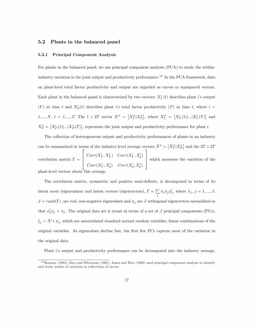
For plants in the balanced panel, we use principal component analysis (PCA) to study the within-

industry variation in the joint output and productivity performance.10 In the PCA framework, data

on plant-level total factor productivity and output are regarded as curves or equispaced vectors.

Each plant in the balanced panel is characterized by two vectors: XiY (t) describes plant i’s output

(Y ) at time t and XiP (t) describes plant i’s total factor productivity (P ) at time t, where i =

1, ..., N , t = 1, ..., T. The 1 × 2T vector Xi0 =£Xi0Y |Xi0

P

¤, where Xi0

Y =£XiY (1)|...|Xi

Y (T )¤and

Xi0P =

£XiP (1)|...|Xi

P (T )¤, represents the joint output and productivity performance for plant i.

The collection of heterogeneous output and productivity performances of plants in an industry

can be summarized in terms of the industry-level average vectors Xi0 =£Xi0Y |Xi0

P

¤and the 2T × 2T

correlation matrix Γ =

⎡⎢⎢⎣ Corr(XiY ,X

iY ) Corr(Xi

Y ,Xip)

Corr(XiY ,X

ip) Corr(Xi

p,Xip)

⎤⎥⎥⎦ which measures the variation of theplant-level vectors about this average.

The correlation matrix, symmetric and positive semi-definite, is decomposed in terms of its

latent roots (eigenvalues) and latent vectors (eigenvectors), Γ =Pjλjφjφ

0j , where λj , j = 1, ..., J ,

J = rank(Γ), are real, non-negative eigenvalues and φj are J orthogonal eigenvectors normalized so

that φ0jφj = λj . The original data set is recast in terms of a set of J principal components (PCs),

ξj = Xi∗ φj , which are uncorrelated standard normal random variables, linear combinations of the

original variables. As eigenvalues decline fast, the first few PCs capture most of the variation in

the original data.

Plant i’s output and productivity performance can be decomposed into the industry average,

10Ramsay (1982), Rice and Silverman (1991), Jones and Rice (1992) used principal component analysis to identifyand study modes of variation in collections of curves.

17

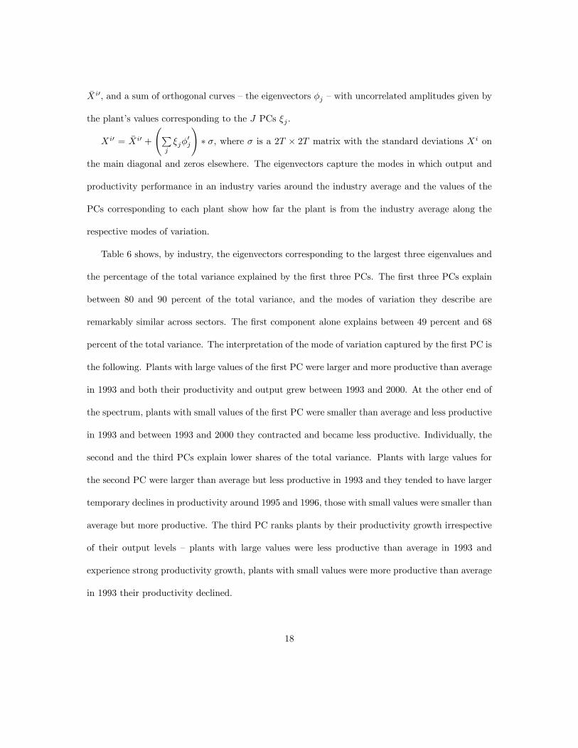
Xi0, and a sum of orthogonal curves — the eigenvectors φj — with uncorrelated amplitudes given by

the plant’s values corresponding to the J PCs ξj .

Xi0 = Xi0 +

ÃPjξjφ

0j

!∗ σ, where σ is a 2T × 2T matrix with the standard deviations Xi on

the main diagonal and zeros elsewhere. The eigenvectors capture the modes in which output and

productivity performance in an industry varies around the industry average and the values of the

PCs corresponding to each plant show how far the plant is from the industry average along the

respective modes of variation.

Table 6 shows, by industry, the eigenvectors corresponding to the largest three eigenvalues and

the percentage of the total variance explained by the first three PCs. The first three PCs explain

between 80 and 90 percent of the total variance, and the modes of variation they describe are

remarkably similar across sectors. The first component alone explains between 49 percent and 68

percent of the total variance. The interpretation of the mode of variation captured by the first PC is

the following. Plants with large values of the first PC were larger and more productive than average

in 1993 and both their productivity and output grew between 1993 and 2000. At the other end of

the spectrum, plants with small values of the first PC were smaller than average and less productive

in 1993 and between 1993 and 2000 they contracted and became less productive. Individually, the

second and the third PCs explain lower shares of the total variance. Plants with large values for

the second PC were larger than average but less productive in 1993 and they tended to have larger

temporary declines in productivity around 1995 and 1996, those with small values were smaller than

average but more productive. The third PC ranks plants by their productivity growth irrespective

of their output levels — plants with large values were less productive than average in 1993 and

experience strong productivity growth, plants with small values were more productive than average

in 1993 their productivity declined.

18

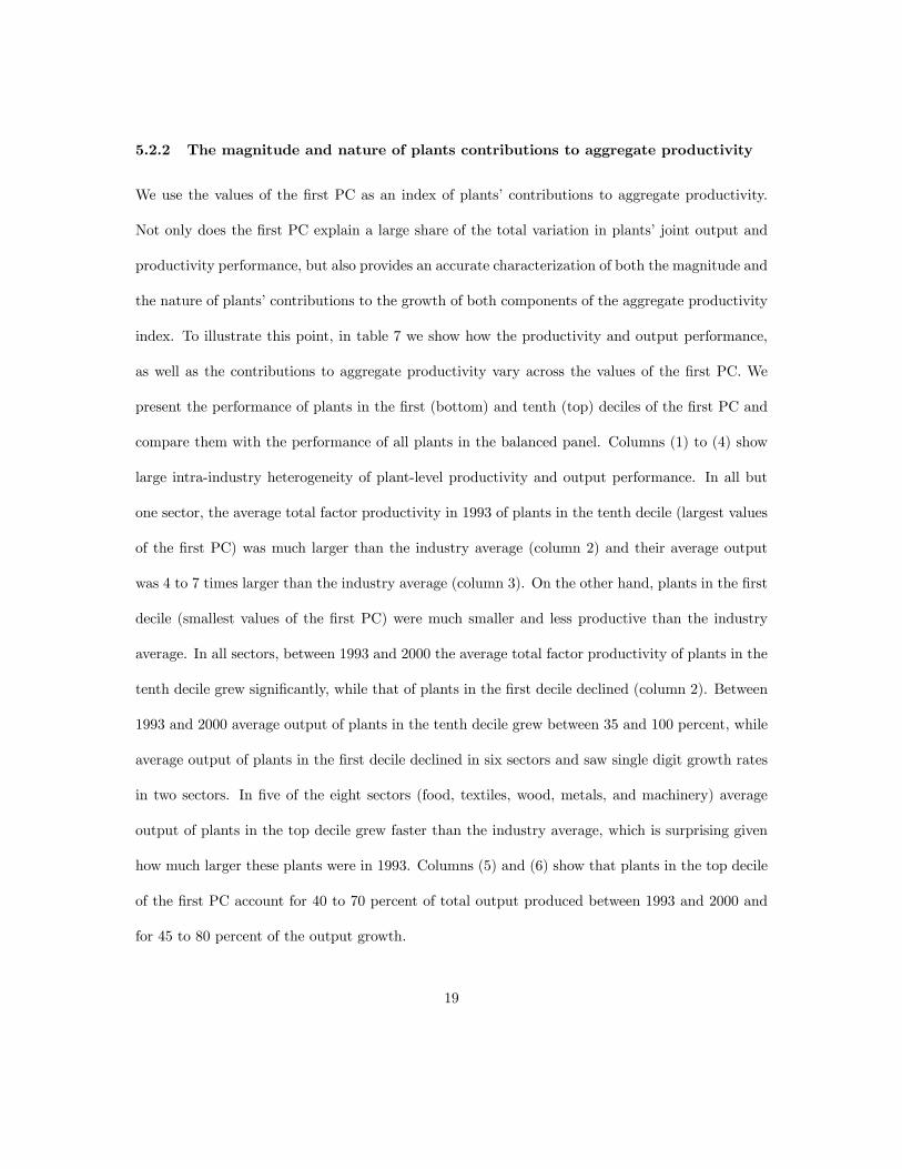
5.2.2 The magnitude and nature of plants contributions to aggregate productivity

We use the values of the first PC as an index of plants’ contributions to aggregate productivity.

Not only does the first PC explain a large share of the total variation in plants’ joint output and

productivity performance, but also provides an accurate characterization of both the magnitude and

the nature of plants’ contributions to the growth of both components of the aggregate productivity

index. To illustrate this point, in table 7 we show how the productivity and output performance,

as well as the contributions to aggregate productivity vary across the values of the first PC. We

present the performance of plants in the first (bottom) and tenth (top) deciles of the first PC and

compare them with the performance of all plants in the balanced panel. Columns (1) to (4) show

large intra-industry heterogeneity of plant-level productivity and output performance. In all but

one sector, the average total factor productivity in 1993 of plants in the tenth decile (largest values

of the first PC) was much larger than the industry average (column 2) and their average output

was 4 to 7 times larger than the industry average (column 3). On the other hand, plants in the first

decile (smallest values of the first PC) were much smaller and less productive than the industry

average. In all sectors, between 1993 and 2000 the average total factor productivity of plants in the

tenth decile grew significantly, while that of plants in the first decile declined (column 2). Between

1993 and 2000 average output of plants in the tenth decile grew between 35 and 100 percent, while

average output of plants in the first decile declined in six sectors and saw single digit growth rates

in two sectors. In five of the eight sectors (food, textiles, wood, metals, and machinery) average

output of plants in the top decile grew faster than the industry average, which is surprising given

how much larger these plants were in 1993. Columns (5) and (6) show that plants in the top decile

of the first PC account for 40 to 70 percent of total output produced between 1993 and 2000 and

for 45 to 80 percent of the output growth.

19

Columns (7) to (12) show the sum of the contributions to aggregate productivity, its components,

and their growth of plants in the top and bottom deciles of the first PC, compared with the overall

contributions of all plants in the balanced panel. Plants in the first decile drive down the unweighted

average productivity (column 7), but since they produce small shares of industry’s output, they have

positive contributions to the covariance component. Their productivity declines and therefore their

contributions to the growth of the unweighted component are negative, but they also contract, which

translates into positive contributions to the growth of the covariance component. The negative

contributions to the unweighted average productivity component and the positive contributions to

the covariance component are of similar magnitudes and, therefore, contributions to the aggregate

productivity growth of plants in the first decile are very small. On the other hand, plants in the

tenth decile account for roughly two thirds of the aggregate productivity growth (by sector shares

vary between 38 percent in paper products and 87 percent in machinery). In all sectors, plants

in the top decile have positive contributions to the unweighted average productivity component

and its growth and to the covariance component and its growth, since they were larger and more

productive in 1993 and both their average productivity and output grew between 1993 and 2000.

5.2.3 Export status and performance

The intra-industry heterogeneity in plants’ productivity and output performance and concentration

of output and aggregate productivity growth, on the one hand, and the sector-level heterogeneity —

industries with large degrees of concentration (like machinery) account for large shares of the overall

manufacturing output and output growth — on the other hand, imply, when considered together,

that most gains accrue to a small number of manufacturing plants. To analyze the way in which

this extraordinary plant-level performance of a small number of plants is related to exporting, we

20

consider two dimensions of exporting activity. The first one is plant’s export status in 1993, before

the implementation of NAFTA. Second, we create a dynamic export status variable that describes

plants’ exporting experience between 1993 and 2000. The dynamic export status variable takes into

account the high incidence of movements into and out of the export market as well as the temporal

patterns displayed by these movements. We construct six types for exporting activity: a) plants

that never export (never), b) plants that always export (always), c) plants that have two or more

spells of exporting during this period (multiple) and three categories of plants that have one spell

of exporting that lasts less than the entire period - d) plants that export in 1993 but stop exporting

before 2000 (stop), e) plants that start exporting after the implementation of NAFTA and export

continuously until 2000 (begin), and f) plants that start exporting after 1993 and stop exporting

before 2000 (temporary). These categories allow us to distinguish, albeit imperfectly,11 among

plants that exit the export market, plants that took advantage of NAFTA to become exporters,

and plants that needed the added effects of NAFTA and exchange rate devaluation to export part

of their output temporarily. For plants with different types of exporting activity, we compare their

productivity and output in 1993, productivity and output growth between 1993 and 2000, and joint

productivity and output performance as described by the first PC.

Table 8 shows the coefficients of simple, sector-level linear regressions with productivity and

output in 1993, and productivity and output growth between 1993 and 2000 as dependent variables

and exporting status in 1993, on the one hand, and the dynamic exporting status, on the other

hand, as independent variables. We present only the coefficients that are significant at 90% level

of confidence. In 1993, before the implementation of NAFTA, exporting plants were larger but not

11We recognize that the distinction we draw here between plants with different dynamic export status is dependenton the relatively short time span of the panel. This classification is simply a convenient description of the eight-yearsegment of plants’ exporting history that we observed in the data set.

21

more productive than non-exporting plants. The coefficients in column (2) in the regression with

output in 1993 as dependent variable are positive and significant in all but one sector, glass. The

coefficients in the regression with productivity in 1993 as dependent variable were not significant,

with the exception of one sector, basic metals, where exporting plants were less productive. In five

out of eight sectors (food, textiles, paper, chemical, and machinery), output growth between 1993

and 2000 was significantly larger at plants that exported before the implementation of NAFTA,

while total factor productivity growth was not significantly different (with the only exception of

basic metals industry).

When we compare coefficients in the regressions with output in 1993 as dependent variable

across specifications, three patterns emerge. First, the magnitudes of the coefficients corresponding

to plants that always export in column (8) are larger than those in column (2) which shows that

plants that always export (always) are selected among the largest 1993 exporters. Second, the

magnitudes of the constant terms in column (3) are smaller than those in column (1) indicating

that plants that never export (never) are selected among the smaller 1993 non-exporters. Third, in

four sectors (food, textiles chemical, glass), plants that began exporting after NAFTA and export

continuously until 2000 (begin) are selected among the larger 1993 non-exporters, while plants with

other types of exporting experience (stop, temporary, and multiple) are not significantly larger than

those that never export.

Among plants with different types of exporting experience, again, only plants that always export

have consistently and significantly larger output growth than plants that never export. Results

with respect to productivity remain weak even when we account for movements into and out of

the export market. Neither productivity in 1993 nor productivity growth between 1993 and 2000

of plants with different types of exporting experience are significantly higher than those of plants

22

that never export.

We analyze two aspects of the relationship between plants’ exporting activities and their joint

productivity and output performance. First, we analyze the makeup of the groups of plants with

best and, respectively, worst output and productivity performance, i.e., the probability distribution

of the types of exporting activity conditional on the values of the first PC. Second, we estimate an

ordered probit model to analyze how the probability of being in each one of the ten deciles of the

first PC is associated with the type of exporting activity, i.e., the probability distribution of the

values of the first PC, conditional on the type of exporting activity.

Table 9 shows, by industry, the distributions of plants with different dynamic exporting status

in the balanced panel and in the first and the tenth deciles of the first PC. While plants that

exported before NAFTA and export continuously through 2000 (always) represent larger fractions

of top-performing plants, the performance of plants with similar exporting experience displays

remarkable heterogeneity. In all industries, plants that never export (never) represent significant

shares of top-performing plants while many exporting plants display poor performance. In five of

the eight sectors plants that always export represent the largest share of plants in the top decile of

the first PC (62 percent in machinery, 61 percent in chemical, 54 percent in textiles, 42 percent in

wood products, and 40 percent in the primary metals sector). In three sectors, plants that never

export represent the largest share of the top performers (42 percent in food products, 37 percent

in glass, and 26 percent in paper products). Plants that begin exporting after 1993 and export

continuously until 2000 (begin) represent the second largest share of top performing plants in six

of the eight sectors. In seven of the eight sectors (the exception is basic metals) plants that never

export represent the largest shares of the plants in the first decile of the first PC — plants with poor

output and productivity performance. Plants that always export, however, represent significant

23

shares of the plants in the first decile in all but two sectors (wood and paper products). Plants

with other types of exporting activity are also found among the worst performing plants in shares

comparable to their share of the balanced panel sample.

Table 10 shows the estimation results for an ordered probit model with deciles of the first PC as

dependent variable and plants’ dynamic exporting status, share of skilled labor, share of imported

inputs, capital intensity, and a binary variable that indicates foreign direct investment in 1993. In

six out of eight sectors (food, textiles, wood, paper, chemicals, and machinery) the coefficients for

plants that always export are positive and significant indicating these plants are more likely to be

found among the plants with better output and productivity performance than plants that never

export. In six of the eight sectors (food, textiles, wood, paper, chemicals, and glass) the coefficients

for plants that begin exporting after 1993 and export continuously until 2000 (begin) are positive

and significant. Controlling for exporting status, capital intensity, foreign direct investment, and the

use of imported inputs are positively correlated with output and productivity performance. Both

the use of imported inputs and foreign direct investment have positive and significant coefficients

in food, chemicals, and machinery sectors, the three sectors with the largest output growth.

Using the estimates from the ordered probit model, we construct the average probabilities of

being in each of the 10 deciles of the first PC, by plants’ dynamic exporting status. Figure 1 shows

the probability profiles by industry. The slope of the probability profile measures the heterogeneity

of the performance of plants with a certain type of exporting activity. Flat profiles — uniform

probability distribution across the deciles of the first PC — indicate a high degree of heterogeneity;

higher positive (negative) slopes indicate relatively higher likelihood of superior (poor) output and

productivity performance. Two patterns emerge from the eight panels. First, in all sectors, the

probability profiles of plants with most types of exporting status fall within a narrow band (0.05 -

24

0.15 probability), which indicates that productivity and ouptut performance of plants with similar

types of exporting activity display strong heterogeneity. Second, plants with two types of exporting

activity depart consistently from this pattern: plants that always export are relatively more likely to

be found among the plants in the top decile and plants that exported in 1993 but stopped exporting

(stop) are relatively more likely to be found in the bottom decile.

The heterogeneous performance of plants with similar exporting activity implies that the re-

duction in the costs of trade provided growth opportunity to larger and more productive plants

irrespective of their export status. The success of plants that sell exclusively on the domestic mar-

ket can have several explanations. The export-driven aggregate growth led to higher incomes and

higher domestic demand, which must have played an important role in sectors like food, paper,

and glass. Higher exports also meant higher demand for intermediary inputs produced by domestic

plants in upstream industries. Finally, stronger import competition forced domestic plants to take

steps to improve their productivity, and plants which were larger and more productive in 1993 were

better positioned to implement efficiency enhancing measures.

While a subset of the exporting plants perform very well, the heterogeneous performance of

plants with similar exporting activity provides an explanation why on average the productivity

performance of exporting plants is not better than that of plants that never export. Several ex-

planations could account for the poor performance of exporting plants during a period in which

NAFTA and the exchange rate devaluation provided favorable exporting conditions. A fair amount

of heterogeneity in the performance of exporting plants could probably be explained by purely idio-

syncratic factors. A portion could also be due to the life cycle of the products — as products become

obsolete, foreign demand declines forcing exporting plants to contract or exit the export market.

Finally, large sunk costs of exporting could create hysteresis of exporting activity. Exporting plants

25

may prefer to incur temporary losses resulting from a decline in demand for their products rather

than exit the foreign markets. Trade liberalization may mitigate this hysteresis effect. It may also

attract more productive infra-marginal plants into exporting, thus shrinking the market for some of

the less productive incumbents and forcing them to contract or exit the foreign market altogether.

6 Conclusion

We use panel data on Mexican manufacturing plants to study the relationship between plants’

responses to changes in the economic environment and their contributions to aggregate productivity

growth in the period following the implementation of NAFTA. Many of our results are consistent

with previous literature on the effect of NAFTA on the performance of the Mexican economy

and with the broader literature on the connection between trade and plant-level and industry-

level performance. Our data show intense export-driven growth in aggregate performance between

1993 and 2000 — the number of exporting plants in the sample grew by almost 50 percent, export

sales doubled, and domestic sales rose by 32 percent. The underlying plant-level behavior displays

remarkable heterogeneity. Some plants contract or exit the market. Others expand by taking

advantage of lower costs of trade to enter export markets or to increase export sales. Changes in

the export activity are heterogeneous both at the extensive margin — plants constantly enter and

exit export markets — and at the intensive margin — exporters increase and decrease export sales by

significant margins. Patterns of entries and exit and changes in intensity depend on the economic

conditions — entries into the export market and increases in exporting intensity are relatively more

prevalent in the period when the effect of NAFTA and the exchange rate devaluation overlap — and

vary across industries.

The complementary changes in export status and changes in export intensity, as well as the

26

simultaneity of entries into and exits from the export market and of intensification and reduction

in exporting activity have been discussed in previous literature. Bernard and Jensen (2004), find

that 60 percent of the export growth is due to changes in exporting intensity at existing exporters,

while Bernard and Jensen (1999) find that 15 percent of today’s exporters will stop exporting next

year and 10 percent of non-exporters will enter foreign markets. What we find more surprising is

how intense exits from the export market and reductions in the exporting intensity remain even

during periods of very favorable exporting conditions. In this respect, our results are consistent

with those in Blalock and Roy (2007), who find that a 2 to 1 devaluation in Indonesian rupiah

caused substantial exit from the export market, exit large enough to offset the growth of exports

at existing exporters and new entries.

Aggregate, industry-level total factor productivity has grown in all industries driven to a large

extent by reallocation of output from the less to more productive plants. Previous literature has

identified international trade — a catalyst of the reallocation process — as a major determinant of the

aggregate productivity growth. In industries with heterogeneous plants and sunk costs of exporting,

more productive plants self-select into exporting; a reduction in the costs of exporting forces least

productive plants in the industry to exit the market, most productive non-exporting plants to

enter export markets, and existing exporters to expand. Our results suggest a picture that differs

in several important respects from these theoretical predictions. First, plant deaths contribute

little to aggregate productivity growth. Plants that exit the market are selected among the least

productive non-exporting plants, but their contributions to the unweighted average productivity

component and to the covariance component are of opposite signs and similar magnitudes. Plants

that exit the market are less productive than the surviving plants long before the actual exit. The

"shadow of death," the relatively long period of contraction preceding exit from the market, makes

27

the actual exit an event of little consequence to the aggregate industry performance.

Second, we find no evidence that plants that exported in 1993 were, on average, more productive

than those that did not export and no evidence that plants with strong exporting performance

between 1993 and 2000 were more productive in 1993 than those that never export in this period.

Plants that exported in 1993, especially those that continued to export until 2000, were larger to

begin with and grew more than those that did not export, but since they were not, on average,

more productive, their expansion could not lead to aggregate productivity growth.

Finally, we do find that strong exporting activity is associated with productivity growth at plant

level, but this connection is shaped by strong plant-level heterogeneity. Aggregate productivity

growth is concentrated in a small fraction of plants. These plants were larger and more productive

in 1993, they grew faster, and, more importantly, became more productive between 1993 and

2000. The group of top-performing plants is very diverse — plants that exported in 1993 and

export continuously through 2000, new entrants into the export market, but also a significant

number of plants that never export — and the distribution of performance is remarkably uniform

within the sets of plants with similar exporting activity. However, plants that export continuously

between 1993 and 2000 and new entrants that export continuously through 2000 have consistently

higher probability of being among the top-performing group than plants that never export. Other

than exporting activity, we found that two factors related to integration into global markets are

consistently correlated with strong output and productivity performance: the use of imported inputs

and foreign investment.

These findings can be rationalized in the context of existing models of exporting decisions.

If there are significant sunk costs of exporting and if returns from exporting are uncertain, then

large plants may be better able to absorb the sunk costs and incur the risks associated with entry

28

into the foreign markets than smaller plants, even very productive ones. Exporting plants, on the

other hand, may find it optimal to accept temporary losses generated by unexpected declines in

foreign demand, rather than exit the export markets. This hysteresis effect implies that, at any

given point in time, many current exporters may be less productive than current non-exporting

plants and that among plants that remain in the export market the dynamics of the performance

is very heterogeneous. The reduction in the costs of trade does not guarantee good performance

for all exporting plants. Trade liberalization reduces the sunk costs of exporting. More productive

infra-marginal plants begin exporting, reducing the market share of less productive incumbents and

forcing them to contract. Lower foreign demand and lower opportunity costs of exiting the foreign

markets induce least productive exporters to cease exporting.

The strong output and productivity growth following the introduction and NAFTA, the exis-

tence of plant-level productivity gains, and the fact that these gains are correlated with exporting

activity, foreign investment, and use of imported inputs suggest that NAFTA has achieved its

goals, and that integration into global markets, in general, helps plants move closer to the inter-

national productivity frontier. The concentration of output and productivity gains in a relatively

small number of plants and the association between foreign investment and use of imported inputs

and plant-level performance indicate that a significant share of the gains from NAFTA accrue to

foreign-owned factors of production.

7 References

Bernard, A., Eaton, J., Jensen, J. B., and Kortum, S. (2003) "Plants and Productivity in Interna-

tional Trade," American Economic Review 93, 1268-1290.

Bernard, A., Jensen, J. B. (1999) “Exceptional exporters performance: cause, effect or both?”

29

Journal of International Economics 47, 1-25.

Bernard, A., Jensen, J. B. (2004) “Why Some Firms Export?” The Review of Economics and

Statistics 86, 561-569.

Bernard, A., Jensen J. B, and Schott, P. K. (2006) ”Trade Costs, Firms, and Productivity”

Journal of Monetary Economics 53, 917-937.

Blalock , G. and Roy, S. (2007) "A firm level examination of theexports puzzlewhy East-Asian

exports did not increase after 1997-1998 financial crisis," The World Economy 30, 39-59.

Greenway, D. and Richard, K. (2007) "Firm Heterogeneity, Exporting and Foreign Direct In-

vestment," The Economic Journal 117, 134-161.

Helpman, E., Melitz, M. and Yeaple, S. (2004) "Export versus FDI,"American Economic Review

94, 300—316.

Jones, M. C. and Rice, J. A. (1992) "Displaying the Important Features of Large Collections of

Similar Curves," The American Statistician 46, 140-145.

Lederman, D., Maloney, W., Serven, L. (2003) “Lessons form NAFTA for Latin American and

Caribbean (LAC) Countries: A Summary of Research Findings," World Bank.

Levinsohn, J. and Petrin, A. (2003) “Estimating Production Functions Using Inputs to Control

For Unobservables,” Review of Economic Studies 70, 317-341.

Lopez-Cordova, E. (2002) “NAFTA and Mexico’s Manufacturing Productivity: An Empirical

Investigation Using Micro-level Data,” mimeo, Inter-American Development Bank, Washington,

D.C.

Melitz, M. J. (2003) "The Impact of Trade on Intra-Industry Reallocations and Aggregate

Industry Productivity," Econometrica 71, 1695-1725.

Olley, S. and Pakes, A. (1996) “The Dynamics of Productivity in the Telecommunications

30

equipment Industry,” Econometrica 64, 1363-1298.

Pavnick, N. (2002) “Trade Liberalization, Exit, and Productivity Improvements: Evidence from

Chilean Plants,” Review of Economic Studies 69, 245-276.

Ramsay, J. O.(1982) "When the Data are Functions," Psychometrika 47, 379-396.

Rice, J. A. and Silverman B.W. (1991) "Estimating the Mean and Covariance Structure Non-

parametrically When the Data are Curves," Journal of the Royal Statistical Society, Series B, 53,

233-243.

Schiff, M. and Wang, Y. (2003) "Regional Integration and Technology Diffusion: The Case of

the North America Free Trade Agreement," World Bank Policy Research Working Paper No. 3132.

Tybout, J. R. (2003) "Plant and firm level evidence on new trade theories," in (E. Kwan Choi

and J. Harrigan, eds.), Handbook of International Economics, 388—415, Oxford: Blackwell.

Tybout, J. and Westbrook, M.D. (1995) “Trade Liberalization and the Dimensions of Efficiency

Change in Mexican Manufacturing Industries,” Journal of International Economics 39, 53-78.

Yeaple S. R. (2003) "Firm Heterogeneity, International Trade, and Wages," University of Penn-

sylvania mimeo.

31

Appendix

A.1. Annual Industrial Survey

AIS uses a non-probabilistic sample drawn from the universe of manufacturing establishments

provided by the 1993 Industrial Census. The sample was selected according to the following two cri-

teria. First, two types of plants were excluded from the sample: establishments that operate under

the special maquiladora regime and petrochemical and oil-refining plants which are state-owned

monopoly. Second, 205 six-digit industries with the largest contribution to total manufacturing

production were selected from a total of 309 six-digit industries.12The largest plants from each in-

dustry, covering at least 80% of the total value of gross production of the industry, were included in

the sample. All remaining plants with at least 100 employees were added to the sample. In classes

where production was highly concentrated, all establishments were included, whereas in classes with

highly disaggregated production maximum 100 establishments were included in the sample. As a

result, the AIS sample includes all the largest plants in the population and a significant share of

medium-scale plants, but a smaller share of small plants and very few micro-enterprises. The AIS

sample has not been refreshed since 1993, but its composition changed every year. Plants were

excluded from the sample for a number of reasons among which, plant closings are well identified.

Plants were added to the sample every year to replace the plants lost.

A.2. Imputation of capital stock

Capital stock is imputed using perpetual inventory method. The replacement value of capital

stock provided by IC is the basis of the imputation procedure. Plants in the data set can be classified

in three categories: plants present in both IC 1993 and IC 1998, plants present in IC 1993 which

12Establishments are classified according to the Mexican Classification of Activities and Products, which at a4-digit level is compatible with the International Uniform Industrial Classification.

32

exit the sample before 1998, and plants which enter the sample between 1993 and 1998, present

only in IC 1998. For all plants which were in present in IC 1993 we impute capital stock using the

replacement value of capital stock in IC 1993 as a basis. For plants which were present in both IC

1993 and IC 1998, we compare the imputed value of capital stock in 1998 with the value of capital

stock in IC 1998 to obtain deflators for each of the seven types of capital stock. Finally, for plants

which initiated operations between 1993 and 1998, and were therefore present only in IC 1998, we

impute capital stock by using the replacement value of capital in IC 1998, appropriately deflated,

as basis.

The second ingredient of the imputation procedure is the rate of depreciation of the capital

stock. We use IC 1998 information on capital stock, investment, sales of capital, and depreciation to

calculate depreciation rates for five types of capital (excluding land), for 70 five-digit manufacturing

sectors. For each firm we calculate depreciation rates for the five types of capital, then median

rates for each of the five-digit sector are chosen. In calculating depreciation rates, it is important to

consider the distribution of investments and sales of capital during the year. The precise timing of

the investments taking place during one year is generally not known and assumptions are necessary

(for example, one can assume that all investments take place at the beginning of the year, at the end

of the year or are uniformly distributed during the year). The assumed timing of the investments

determines the denominator of the depreciation rate and, hence, the size of the depreciation rate.

In this paper we assume both investments and sales of capital are uniformly distributed during the

year.

Investments and sales of capital are the third ingredient of the imputation procedure. From AIS

we extracted information on investments for two groups of capital stock types. First group pools

together machinery, transportation equipment, computing and peripheral equipment, and furniture

33

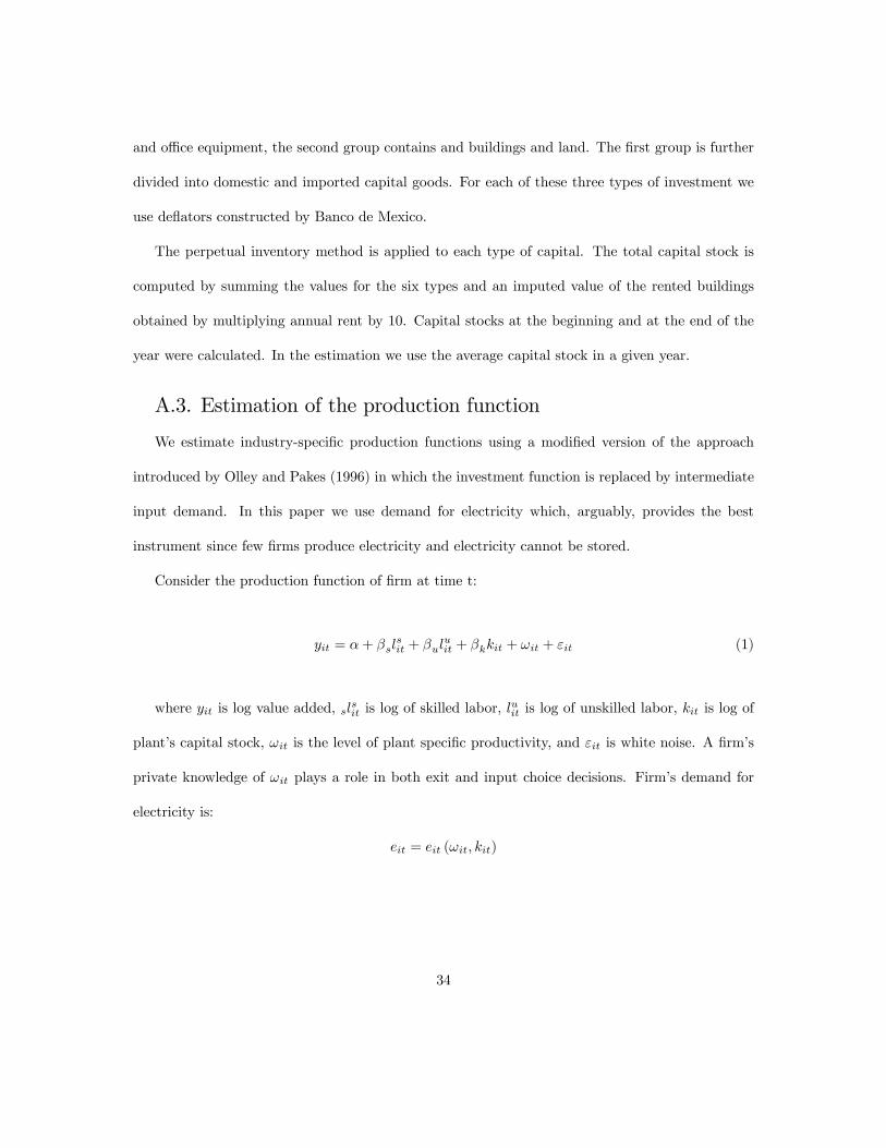
and office equipment, the second group contains and buildings and land. The first group is further

divided into domestic and imported capital goods. For each of these three types of investment we

use deflators constructed by Banco de Mexico.

The perpetual inventory method is applied to each type of capital. The total capital stock is

computed by summing the values for the six types and an imputed value of the rented buildings

obtained by multiplying annual rent by 10. Capital stocks at the beginning and at the end of the

year were calculated. In the estimation we use the average capital stock in a given year.

A.3. Estimation of the production function

We estimate industry-specific production functions using a modified version of the approach

introduced by Olley and Pakes (1996) in which the investment function is replaced by intermediate

input demand. In this paper we use demand for electricity which, arguably, provides the best

instrument since few firms produce electricity and electricity cannot be stored.

Consider the production function of firm at time t:

yit = α+ βslsit + βul

uit + βkkit + ωit + εit (1)

where yit is log value added, slsit is log of skilled labor, luit is log of unskilled labor, kit is log of

plant’s capital stock, ωit is the level of plant specific productivity, and εit is white noise. A firm’s

private knowledge of ωit plays a role in both exit and input choice decisions. Firm’s demand for

electricity is:

eit = eit (ωit, kit)

34

Under monotonicity conditions, the demand function can be inverted,

ωit = ωit (eit, kit)

Replacing ωit, (1) becomes:

yit = βslsit + βul

uit + φ (eit, kit) + εit (2)

where φ (eit, kit) = α+ βkkit + ωit

In the first step we use OLS to estimate βs and βu in (2) where φ (eit, kit) is represented by a

polynomial expansion in eit and kit. Using the coefficient estimates at the first step, we calculate

an estimate for φ (eit, kit), φ (eit, kit) = yit − βslsit − βul

uit

Let

y∗it+1 = yit+1 − βslsit+1 − βul

uit+1 = α+ βkkit+1 + ωit+1 + εit+1 (3)

To address the selection bias problem, firm’s exit decision is specifically modelled. Writing the

realization of the new productivity shock as a sum of a forecasted component and an idiosyncratic

component, ωit+1 = E [ωit+1|ωit] + ηit+1,and denoting g (ωit) = α + E [ωit+1|ωit], equation 3

becomes

y∗it+1 = βkkit+1 + g (ωit) + εit+1

A firm is observed only if the realization of productivity is above a certain threshold. The firms

35

exit decision is then represented by:

Xt = 1 if ωt > ωt

Xt = 0 otherwise

Incorporating the exit decision, (3) becomes:

y∗it+1 = yit+1 − βslsit+1 − βul

uit+1 =

= α+ βkkit+1 +Ehωit+1|ωit, ωt+1 > ωt+1

i+ ηit+1 + εit+1

The second estimation step is then:

y∗it+1 = yit+1 − βslsit+1 − βul

uit+1 =

= βkkit+1 + g³φ (eit, kit)− βkkit, Pit

´+ ηit+1 + εit+1 (4)

We use a polynomial expansion for g,

g³φ (eit, kit)− βkkit, Pit

´=Pj

Pl

βjl

³φ (eit, kit)− βkkit

´jP lit and non-linear least square to

estimate (4).

Finally, using the coefficient estimates from the two steps of the estimation, we calculate total

factor productivity as

ωit = yit − βslsit − βul

uit − βkkit

36

Sector

Food Exp. plants 138 (19.4%) 158 (22.4%) 181 (25.9%) 209 (30.4%) 226 (33.4%) 213 (31.6%) 225 (33.4%) 214 (31.8%) 76 (55.1%)Exp. Sales 2.36 (3.1%) 2.57 (3.3%) 4.26 (5.5%) 4.91 (6.1%) 5.49 (6.3%) 6.70 (7.2%) 6.86 (6.8%) 6.40 (6.1%) 4.05 (171.9%)Dom. sales 72.61 (96.9%) 76.32 (96.7%) 72.91 (94.5%) 76.15 (93.9%) 81.04 (93.7%) 86.83 (92.8%) 93.36 (93.2%) 98.74 (93.9%) 26.14 (36.0%)

Textiles Exp. plants 175 (26.5%) 164 (25.4%) 256 (41.3%) 288 (48.7%) 302 (54.2%) 276 (49.8%) 283 (51.4%) 274 (49.7%) 99 (56.6%)Exp. Sales 1.12 (8.1%) 1.08 (7.7%) 2.26 (17.0%) 2.91 (18.3%) 3.38 (19.8%) 3.28 (19.1%) 3.18 (18.3%) 3.15 (17.8%) 2.03 (181.2%)Dom. sales 12.74 (91.9%) 13.00 (92.3%) 11.01 (83.0%) 12.99 (81.7%) 13.70 (80.2%) 13.93 (80.9%) 14.13 (81.7%) 14.53 (82.2%) 1.78 (14.0%)

Wood Exp. plants 21 (14.7%) 19 (13.5%) 39 (28.9%) 50 (39.4%) 52 (42.3%) 46 (37.4%) 44 (36.1%) 47 (38.5%) 26 (123.8%)Exp. Sales 0.12 (6.4%) 0.20 (9.6%) 0.38 (20.8%) 0.52 (24.1%) 0.59 (24.5%) 0.61 (24.0%) 0.58 (22.3%) 0.49 (18.8%) 0.37 (294.1%)Dom. sales 1.81 (93.6%) 1.85 (90.4%) 1.45 (79.2%) 1.64 (75.9%) 1.82 (75.5%) 1.92 (76.0%) 2.02 (77.7%) 2.12 (81.2%) 0.31 (17.2%)

Paper Exp. plants 63 (19.9%) 59 (18.8%) 70 (22.6%) 78 (25.4%) 78 (25.5%) 70 (23.0%) 81 (26.6%) 83 (27.2%) 20 (31.7%)Exp. Sales 0.21 (1.5%) 0.27 (1.8%) 0.66 (4.6%) 0.45 (3.0%) 0.47 (2.8%) 0.61 (3.4%) 0.50 (2.7%) 0.45 (2.4%) 0.24 (113.0%)Dom. sales 13.72 (98.5%) 14.50 (98.2%) 13.46 (95.4%) 14.49 (97.0%) 16.38 (97.2%) 17.08 (96.6%) 17.87 (97.3%) 18.33 (97.6%) 4.61 (33.6%)

Chemical Exp. plants 320 (37.8%) 326 (38.9%) 374 (45.5%) 408 (50.5%) 432 (54.1%) 424 (52.9%) 429 (53.6%) 444 (55.5%) 124 (38.8%)Exp. Sales 6.17 (13.0%) 7.68 (14.8%) 10.66 (20.9%) 10.53 (18.9%) 10.89 (17.4%) 11.17 (16.9%) 12.00 (17.9%) 12.46 (17.6%) 6.29 (101.9%)Dom. sales 41.43 (87.0%) 44.11 (85.2%) 40.24 (79.1%) 45.14 (81.1%) 51.65 (82.6%) 55.07 (83.1%) 54.97 (82.1%) 58.37 (82.4%) 16.94 (40.9%)

Glass Exp. plants 68 (23.7%) 75 (27.3%) 86 (32.6%) 89 (35.0%) 94 (38.4%) 88 (36.2%) 97 (40.1%) 91 (37.6%) 23 (33.8%)Exp. Sales 1.11 (6.7%) 1.59 (8.7%) 2.45 (15.2%) 2.64 (14.9%) 2.80 (14.7%) 2.72 (13.5%) 2.66 (12.6%) 2.76 (12.5%) 1.66 (149.3%)Dom. sales 15.47 (93.3%) 16.62 (91.3%) 13.62 (84.8%) 15.12 (85.1%) 16.28 (85.3%) 17.47 (86.5%) 18.40 (87.4%) 19.44 (87.5%) 3.97 (25.7%)

Metals Exp. plants 40 (36.7%) 48 (45.3%) 63 (61.8%) 64 (62.1%) 62 (62.0%) 61 (61.0%) 65 (65.0%) 65 (65.0%) 25 (62.5%)Exp. Sales 4.11 (17.8%) 4.39 (17.4%) 9.75 (33.0%) 8.07 (24.3%) 8.40 (22.5%) 8.29 (22.8%) 7.85 (21.5%) 8.05 (21.6%) 3.94 (96.0%)Dom. sales 18.93 (82.2%) 20.88 (82.6%) 19.78 (67.0%) 25.09 (75.7%) 28.87 (77.5%) 28.08 (77.2%) 28.63 (78.5%) 29.18 (78.4%) 10.26 (54.2%)

Machinery Exp. plants 398 (40.4%) 410 (41.9%) 488 (51.2%) 522 (56.7%) 553 (61.5%) 555 (62.0%) 561 (63.0%) 558 (62.7%) 160 (40.2%)Exp. Sales 27.99 (32.9%) 33.86 (37.5%) 44.92 (58.2%) 57.75 (58.9%) 63.21 (54.7%) 68.39 (54.7%) 74.96 (55.9%) 92.37 (57.7%) 64.38 (230.0%)Dom. sales 57.03 (67.1%) 56.44 (62.5%) 32.27 (41.8%) 40.35 (41.1%) 52.35 (45.3%) 56.69 (45.3%) 59.24 (44.1%) 67.66 (42.3%) 10.63 (18.6%)

Total Exp. plants 1223 (30.1%) 1259 (31.4%) 1557 (39.9%) 1708 (45.0%) 1799 (48.5%) 1733 (46.9%) 1785 (48.5%) 1776 (48.2%) 553 (45.2%)Exp. Sales 43 (15.6%) 52 (17.5%) 75 (26.9%) 88 (27.5%) 95 (26.7%) 102 (26.9%) 109 (27.3%) 126 (29.0%) 82.95 (192.0%)Dom. sales 234 (84.4%) 244 (82.5%) 205 (73.1%) 231 (72.5%) 262 (73.3%) 277 (73.1%) 289 (72.7%) 308 (71.0%) 74.64 (31.9%)

Note: Sales are measured in billion 1993 pesos

1999 2000 1993-2000

Change (% )

Table 1. Total, domestic, and export sales by industry, 1993-2000

1993 1994 1995 1996 1997 1998

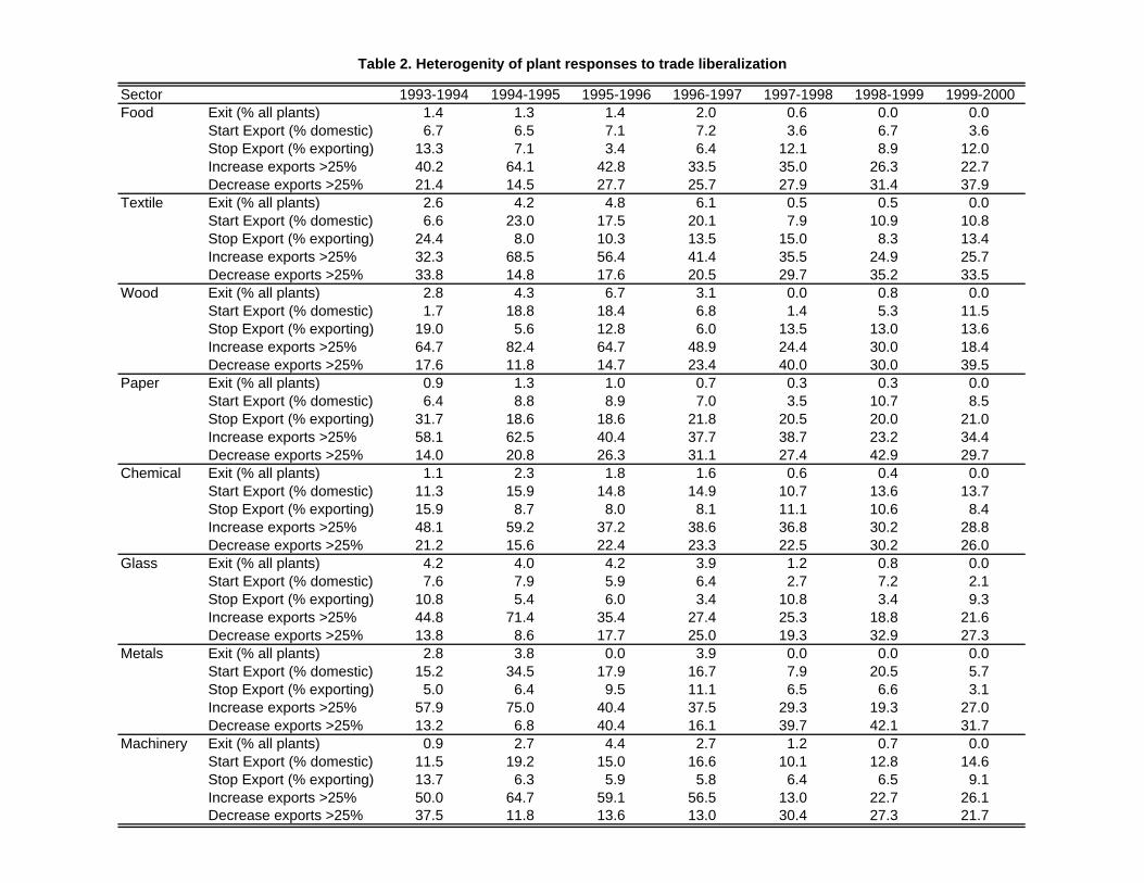
SectorFood Exit (% all plants) 1.4 1.3 1.4 2.0 0.6 0.0 0.0

Start Export (% domestic) 6.7 6.5 7.1 7.2 3.6 6.7 3.6Stop Export (% exporting) 13.3 7.1 3.4 6.4 12.1 8.9 12.0Increase exports >25% 40.2 64.1 42.8 33.5 35.0 26.3 22.7Decrease exports >25% 21.4 14.5 27.7 25.7 27.9 31.4 37.9

Textile Exit (% all plants) 2.6 4.2 4.8 6.1 0.5 0.5 0.0Start Export (% domestic) 6.6 23.0 17.5 20.1 7.9 10.9 10.8Stop Export (% exporting) 24.4 8.0 10.3 13.5 15.0 8.3 13.4Increase exports >25% 32.3 68.5 56.4 41.4 35.5 24.9 25.7Decrease exports >25% 33.8 14.8 17.6 20.5 29.7 35.2 33.5

Wood Exit (% all plants) 2.8 4.3 6.7 3.1 0.0 0.8 0.0Start Export (% domestic) 1.7 18.8 18.4 6.8 1.4 5.3 11.5Stop Export (% exporting) 19.0 5.6 12.8 6.0 13.5 13.0 13.6Increase exports >25% 64.7 82.4 64.7 48.9 24.4 30.0 18.4Decrease exports >25% 17.6 11.8 14.7 23.4 40.0 30.0 39.5

Paper Exit (% all plants) 0.9 1.3 1.0 0.7 0.3 0.3 0.0Start Export (% domestic) 6.4 8.8 8.9 7.0 3.5 10.7 8.5Stop Export (% exporting) 31.7 18.6 18.6 21.8 20.5 20.0 21.0Increase exports >25% 58.1 62.5 40.4 37.7 38.7 23.2 34.4Decrease exports >25% 14.0 20.8 26.3 31.1 27.4 42.9 29.7

Chemical Exit (% all plants) 1.1 2.3 1.8 1.6 0.6 0.4 0.0Start Export (% domestic) 11.3 15.9 14.8 14.9 10.7 13.6 13.7Stop Export (% exporting) 15.9 8.7 8.0 8.1 11.1 10.6 8.4Increase exports >25% 48.1 59.2 37.2 38.6 36.8 30.2 28.8Decrease exports >25% 21.2 15.6 22.4 23.3 22.5 30.2 26.0

Glass Exit (% all plants) 4.2 4.0 4.2 3.9 1.2 0.8 0.0Start Export (% domestic) 7.6 7.9 5.9 6.4 2.7 7.2 2.1Stop Export (% exporting) 10.8 5.4 6.0 3.4 10.8 3.4 9.3Increase exports >25% 44.8 71.4 35.4 27.4 25.3 18.8 21.6Decrease exports >25% 13.8 8.6 17.7 25.0 19.3 32.9 27.3

Metals Exit (% all plants) 2.8 3.8 0.0 3.9 0.0 0.0 0.0Start Export (% domestic) 15.2 34.5 17.9 16.7 7.9 20.5 5.7Stop Export (% exporting) 5.0 6.4 9.5 11.1 6.5 6.6 3.1Increase exports >25% 57.9 75.0 40.4 37.5 29.3 19.3 27.0Decrease exports >25% 13.2 6.8 40.4 16.1 39.7 42.1 31.7

Machinery Exit (% all plants) 0.9 2.7 4.4 2.7 1.2 0.7 0.0Start Export (% domestic) 11.5 19.2 15.0 16.6 10.1 12.8 14.6Stop Export (% exporting) 13.7 6.3 5.9 5.8 6.4 6.5 9.1Increase exports >25% 50.0 64.7 59.1 56.5 13.0 22.7 26.1Decrease exports >25% 37.5 11.8 13.6 13.0 30.4 27.3 21.7

1999-2000

Table 2. Heterogenity of plant responses to trade liberalization

1993-1994 1994-1995 1995-1996 1996-1997 1997-1998 1998-1999

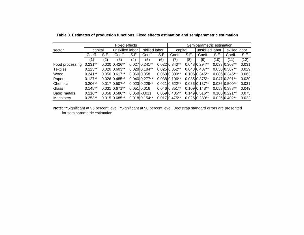
Table 3. Estimates of production functions. Fixed effects estimation and semiparametric estimation

sectorCoeff. S.E. Coeff. S.E Coeff. S.E Coeff. S.E. Coeff. S.E Coeff. S.E

(1) (2) (3) (4) (5) (6) (7) (8) (9) (10) (11) (12)Food processing 0.231** 0.020 0.426** 0.027 0.241** 0.022 0.340** 0.048 0.294** 0.033 0.303** 0.031Textiles 0.123** 0.020 0.603** 0.028 0.184** 0.025 0.352** 0.043 0.487** 0.030 0.307** 0.029Wood 0.241** 0.050 0.617** 0.060 0.058 0.060 0.380** 0.106 0.345** 0.086 0.345** 0.063Paper 0.127** 0.026 0.485** 0.040 0.277** 0.038 0.196** 0.085 0.375** 0.047 0.391** 0.030Chemical 0.206** 0.017 0.507** 0.023 0.229** 0.021 0.522** 0.036 0.137** 0.036 0.500** 0.031Glass 0.145** 0.031 0.671** 0.051 0.016 0.046 0.351** 0.109 0.148** 0.053 0.388** 0.049Basic metals 0.116** 0.058 0.586** 0.058 -0.011 0.059 0.485** 0.149 0.516** 0.100 0.221** 0.075Machinery 0.253** 0.015 0.685** 0.018 0.154** 0.017 0.475** 0.026 0.289** 0.025 0.402** 0.022

Note: **Significant at 95 percent level. *Significant at 90 percent level. Bootstrap standard errors are presented for semiparametric estimation

Fixed effects Semiparametric estimationcapital unskilled labor skilled labor capital unskilled labor skilled labor

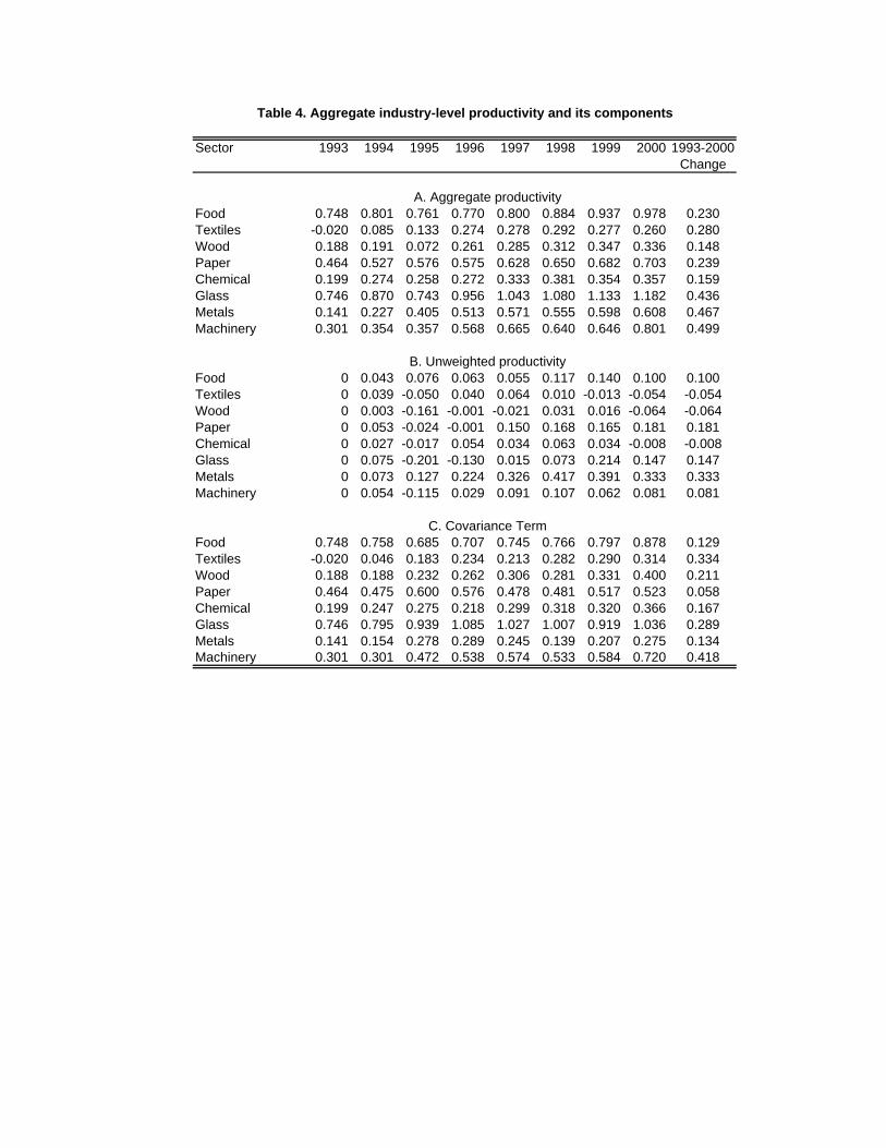
Sector 1993 1994 1995 1996 1997 1998 1999 2000 1993-2000Change

Food 0.748 0.801 0.761 0.770 0.800 0.884 0.937 0.978 0.230Textiles -0.020 0.085 0.133 0.274 0.278 0.292 0.277 0.260 0.280Wood 0.188 0.191 0.072 0.261 0.285 0.312 0.347 0.336 0.148Paper 0.464 0.527 0.576 0.575 0.628 0.650 0.682 0.703 0.239Chemical 0.199 0.274 0.258 0.272 0.333 0.381 0.354 0.357 0.159Glass 0.746 0.870 0.743 0.956 1.043 1.080 1.133 1.182 0.436Metals 0.141 0.227 0.405 0.513 0.571 0.555 0.598 0.608 0.467Machinery 0.301 0.354 0.357 0.568 0.665 0.640 0.646 0.801 0.499

Food 0 0.043 0.076 0.063 0.055 0.117 0.140 0.100 0.100Textiles 0 0.039 -0.050 0.040 0.064 0.010 -0.013 -0.054 -0.054Wood 0 0.003 -0.161 -0.001 -0.021 0.031 0.016 -0.064 -0.064Paper 0 0.053 -0.024 -0.001 0.150 0.168 0.165 0.181 0.181Chemical 0 0.027 -0.017 0.054 0.034 0.063 0.034 -0.008 -0.008Glass 0 0.075 -0.201 -0.130 0.015 0.073 0.214 0.147 0.147Metals 0 0.073 0.127 0.224 0.326 0.417 0.391 0.333 0.333Machinery 0 0.054 -0.115 0.029 0.091 0.107 0.062 0.081 0.081

Food 0.748 0.758 0.685 0.707 0.745 0.766 0.797 0.878 0.129Textiles -0.020 0.046 0.183 0.234 0.213 0.282 0.290 0.314 0.334Wood 0.188 0.188 0.232 0.262 0.306 0.281 0.331 0.400 0.211Paper 0.464 0.475 0.600 0.576 0.478 0.481 0.517 0.523 0.058Chemical 0.199 0.247 0.275 0.218 0.299 0.318 0.320 0.366 0.167Glass 0.746 0.795 0.939 1.085 1.027 1.007 0.919 1.036 0.289Metals 0.141 0.154 0.278 0.289 0.245 0.139 0.207 0.275 0.134Machinery 0.301 0.301 0.472 0.538 0.574 0.533 0.584 0.720 0.418

B. Unweighted productivity

C. Covariance Term

A. Aggregate productivity

Table 4. Aggregate industry-level productivity and its components

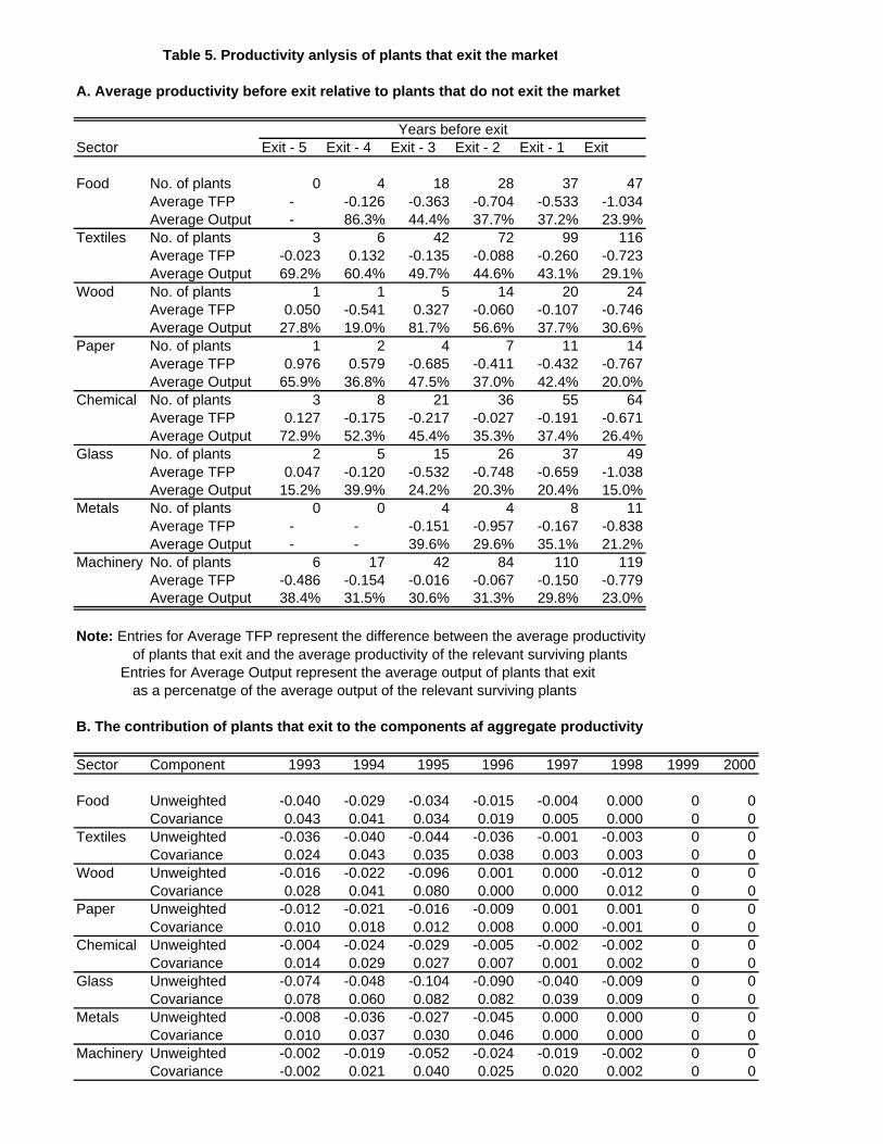
A. Average productivity before exit relative to plants that do not exit the market

Sector Exit - 5 Exit - 4 Exit - 3 Exit - 2 Exit - 1 Exit

Food No. of plants 0 4 18 28 37 47Average TFP - -0.126 -0.363 -0.704 -0.533 -1.034Average Output - 86.3% 44.4% 37.7% 37.2% 23.9%

Textiles No. of plants 3 6 42 72 99 116Average TFP -0.023 0.132 -0.135 -0.088 -0.260 -0.723Average Output 69.2% 60.4% 49.7% 44.6% 43.1% 29.1%

Wood No. of plants 1 1 5 14 20 24Average TFP 0.050 -0.541 0.327 -0.060 -0.107 -0.746Average Output 27.8% 19.0% 81.7% 56.6% 37.7% 30.6%

Paper No. of plants 1 2 4 7 11 14Average TFP 0.976 0.579 -0.685 -0.411 -0.432 -0.767Average Output 65.9% 36.8% 47.5% 37.0% 42.4% 20.0%

Chemical No. of plants 3 8 21 36 55 64Average TFP 0.127 -0.175 -0.217 -0.027 -0.191 -0.671Average Output 72.9% 52.3% 45.4% 35.3% 37.4% 26.4%

Glass No. of plants 2 5 15 26 37 49Average TFP 0.047 -0.120 -0.532 -0.748 -0.659 -1.038Average Output 15.2% 39.9% 24.2% 20.3% 20.4% 15.0%

Metals No. of plants 0 0 4 4 8 11Average TFP - - -0.151 -0.957 -0.167 -0.838Average Output - - 39.6% 29.6% 35.1% 21.2%

Machinery No. of plants 6 17 42 84 110 119Average TFP -0.486 -0.154 -0.016 -0.067 -0.150 -0.779Average Output 38.4% 31.5% 30.6% 31.3% 29.8% 23.0%

Note: Entries for Average TFP represent the difference between the average productivity of plants that exit and the average productivity of the relevant surviving plants Entries for Average Output represent the average output of plants that exit as a percenatge of the average output of the relevant surviving plants

B. The contribution of plants that exit to the components af aggregate productivity

Sector Component 1993 1994 1995 1996 1997 1998 1999 2000

Food Unweighted -0.040 -0.029 -0.034 -0.015 -0.004 0.000 0 0Covariance 0.043 0.041 0.034 0.019 0.005 0.000 0 0

Textiles Unweighted -0.036 -0.040 -0.044 -0.036 -0.001 -0.003 0 0Covariance 0.024 0.043 0.035 0.038 0.003 0.003 0 0

Wood Unweighted -0.016 -0.022 -0.096 0.001 0.000 -0.012 0 0Covariance 0.028 0.041 0.080 0.000 0.000 0.012 0 0

Paper Unweighted -0.012 -0.021 -0.016 -0.009 0.001 0.001 0 0Covariance 0.010 0.018 0.012 0.008 0.000 -0.001 0 0

Chemical Unweighted -0.004 -0.024 -0.029 -0.005 -0.002 -0.002 0 0Covariance 0.014 0.029 0.027 0.007 0.001 0.002 0 0

Glass Unweighted -0.074 -0.048 -0.104 -0.090 -0.040 -0.009 0 0Covariance 0.078 0.060 0.082 0.082 0.039 0.009 0 0

Metals Unweighted -0.008 -0.036 -0.027 -0.045 0.000 0.000 0 0Covariance 0.010 0.037 0.030 0.046 0.000 0.000 0 0

Machinery Unweighted -0.002 -0.019 -0.052 -0.024 -0.019 -0.002 0 0Covariance -0.002 0.021 0.040 0.025 0.020 0.002 0 0

Years before exit

Table 5. Productivity anlysis of plants that exit the market

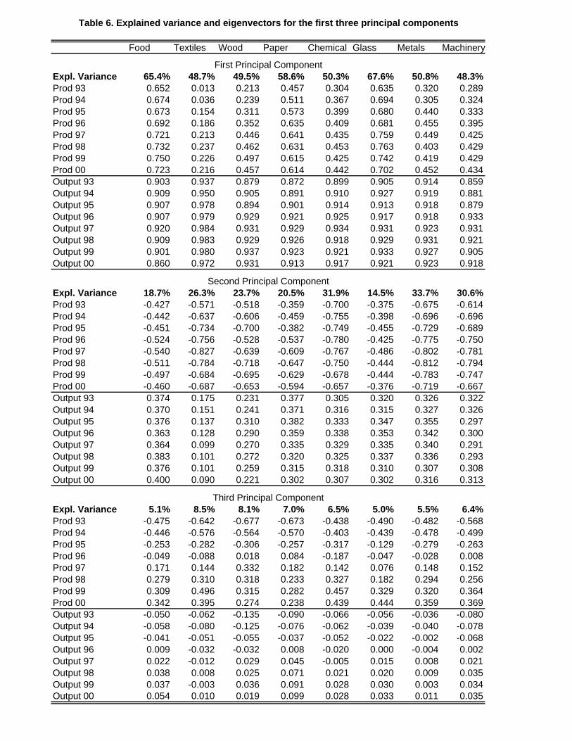
Food Textiles Wood Paper Chemical Glass Metals Machinery

Expl. Variance 65.4% 48.7% 49.5% 58.6% 50.3% 67.6% 50.8% 48.3%Prod 93 0.652 0.013 0.213 0.457 0.304 0.635 0.320 0.289Prod 94 0.674 0.036 0.239 0.511 0.367 0.694 0.305 0.324Prod 95 0.673 0.154 0.311 0.573 0.399 0.680 0.440 0.333Prod 96 0.692 0.186 0.352 0.635 0.409 0.681 0.455 0.395Prod 97 0.721 0.213 0.446 0.641 0.435 0.759 0.449 0.425Prod 98 0.732 0.237 0.462 0.631 0.453 0.763 0.403 0.429Prod 99 0.750 0.226 0.497 0.615 0.425 0.742 0.419 0.429Prod 00 0.723 0.216 0.457 0.614 0.442 0.702 0.452 0.434Output 93 0.903 0.937 0.879 0.872 0.899 0.905 0.914 0.859Output 94 0.909 0.950 0.905 0.891 0.910 0.927 0.919 0.881Output 95 0.907 0.978 0.894 0.901 0.914 0.913 0.918 0.879Output 96 0.907 0.979 0.929 0.921 0.925 0.917 0.918 0.933Output 97 0.920 0.984 0.931 0.929 0.934 0.931 0.923 0.931Output 98 0.909 0.983 0.929 0.926 0.918 0.929 0.931 0.921Output 99 0.901 0.980 0.937 0.923 0.921 0.933 0.927 0.905Output 00 0.860 0.972 0.931 0.913 0.917 0.921 0.923 0.918

Expl. Variance 18.7% 26.3% 23.7% 20.5% 31.9% 14.5% 33.7% 30.6%Prod 93 -0.427 -0.571 -0.518 -0.359 -0.700 -0.375 -0.675 -0.614Prod 94 -0.442 -0.637 -0.606 -0.459 -0.755 -0.398 -0.696 -0.696Prod 95 -0.451 -0.734 -0.700 -0.382 -0.749 -0.455 -0.729 -0.689Prod 96 -0.524 -0.756 -0.528 -0.537 -0.780 -0.425 -0.775 -0.750Prod 97 -0.540 -0.827 -0.639 -0.609 -0.767 -0.486 -0.802 -0.781Prod 98 -0.511 -0.784 -0.718 -0.647 -0.750 -0.444 -0.812 -0.794Prod 99 -0.497 -0.684 -0.695 -0.629 -0.678 -0.444 -0.783 -0.747Prod 00 -0.460 -0.687 -0.653 -0.594 -0.657 -0.376 -0.719 -0.667Output 93 0.374 0.175 0.231 0.377 0.305 0.320 0.326 0.322Output 94 0.370 0.151 0.241 0.371 0.316 0.315 0.327 0.326Output 95 0.376 0.137 0.310 0.382 0.333 0.347 0.355 0.297Output 96 0.363 0.128 0.290 0.359 0.338 0.353 0.342 0.300Output 97 0.364 0.099 0.270 0.335 0.329 0.335 0.340 0.291Output 98 0.383 0.101 0.272 0.320 0.325 0.337 0.336 0.293Output 99 0.376 0.101 0.259 0.315 0.318 0.310 0.307 0.308Output 00 0.400 0.090 0.221 0.302 0.307 0.302 0.316 0.313

Expl. Variance 5.1% 8.5% 8.1% 7.0% 6.5% 5.0% 5.5% 6.4%Prod 93 -0.475 -0.642 -0.677 -0.673 -0.438 -0.490 -0.482 -0.568Prod 94 -0.446 -0.576 -0.564 -0.570 -0.403 -0.439 -0.478 -0.499Prod 95 -0.253 -0.282 -0.306 -0.257 -0.317 -0.129 -0.279 -0.263Prod 96 -0.049 -0.088 0.018 0.084 -0.187 -0.047 -0.028 0.008Prod 97 0.171 0.144 0.332 0.182 0.142 0.076 0.148 0.152Prod 98 0.279 0.310 0.318 0.233 0.327 0.182 0.294 0.256Prod 99 0.309 0.496 0.315 0.282 0.457 0.329 0.320 0.364Prod 00 0.342 0.395 0.274 0.238 0.439 0.444 0.359 0.369Output 93 -0.050 -0.062 -0.135 -0.090 -0.066 -0.056 -0.036 -0.080Output 94 -0.058 -0.080 -0.125 -0.076 -0.062 -0.039 -0.040 -0.078Output 95 -0.041 -0.051 -0.055 -0.037 -0.052 -0.022 -0.002 -0.068Output 96 0.009 -0.032 -0.032 0.008 -0.020 0.000 -0.004 0.002Output 97 0.022 -0.012 0.029 0.045 -0.005 0.015 0.008 0.021Output 98 0.038 0.008 0.025 0.071 0.021 0.020 0.009 0.035Output 99 0.037 -0.003 0.036 0.091 0.028 0.030 0.003 0.034Output 00 0.054 0.010 0.019 0.099 0.028 0.033 0.011 0.035

First Principal Component

Second Principal Component

Third Principal Component

Table 6. Explained variance and eigenvectors for the first three principal components

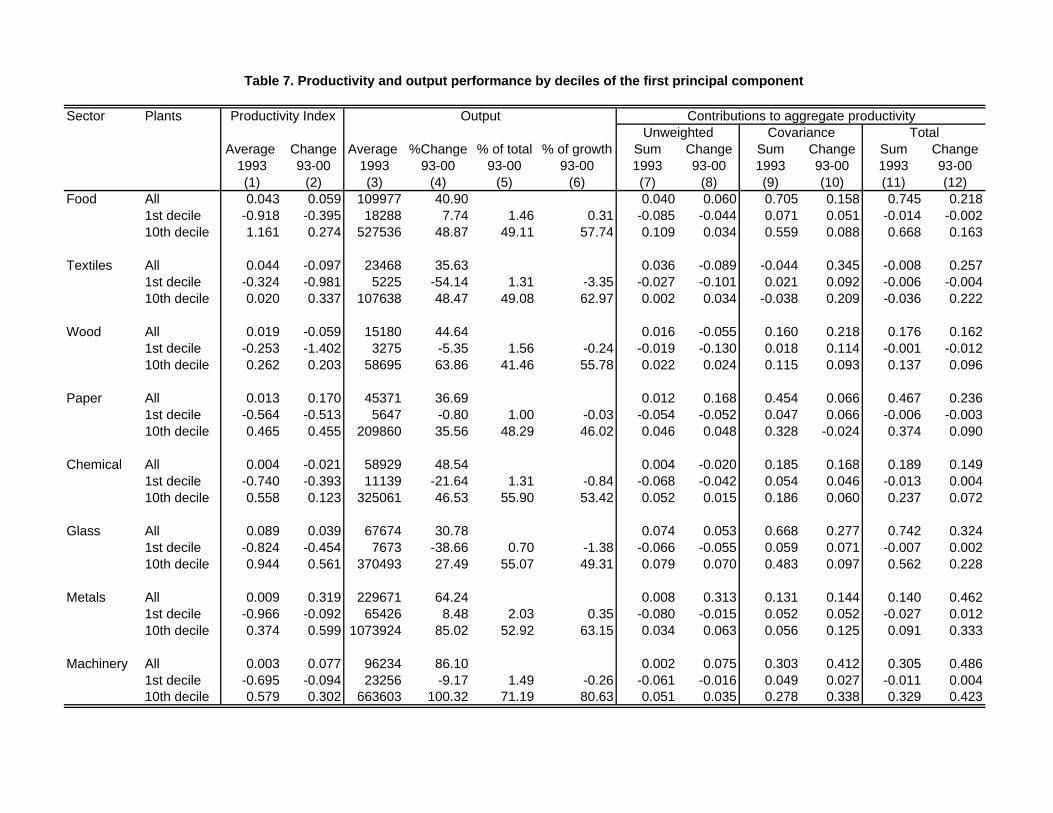
Sector Plants

Average Change Average %Change % of total % of growth Sum Change Sum Change Sum Change1993 93-00 1993 93-00 93-00 93-00 1993 93-00 1993 93-00 1993 93-00(1) (2) (3) (4) (5) (6) (7) (8) (9) (10) (11) (12)

Food All 0.043 0.059 109977 40.90 0.040 0.060 0.705 0.158 0.745 0.2181st decile -0.918 -0.395 18288 7.74 1.46 0.31 -0.085 -0.044 0.071 0.051 -0.014 -0.00210th decile 1.161 0.274 527536 48.87 49.11 57.74 0.109 0.034 0.559 0.088 0.668 0.163

Textiles All 0.044 -0.097 23468 35.63 0.036 -0.089 -0.044 0.345 -0.008 0.2571st decile -0.324 -0.981 5225 -54.14 1.31 -3.35 -0.027 -0.101 0.021 0.092 -0.006 -0.00410th decile 0.020 0.337 107638 48.47 49.08 62.97 0.002 0.034 -0.038 0.209 -0.036 0.222

Wood All 0.019 -0.059 15180 44.64 0.016 -0.055 0.160 0.218 0.176 0.1621st decile -0.253 -1.402 3275 -5.35 1.56 -0.24 -0.019 -0.130 0.018 0.114 -0.001 -0.01210th decile 0.262 0.203 58695 63.86 41.46 55.78 0.022 0.024 0.115 0.093 0.137 0.096

Paper All 0.013 0.170 45371 36.69 0.012 0.168 0.454 0.066 0.467 0.2361st decile -0.564 -0.513 5647 -0.80 1.00 -0.03 -0.054 -0.052 0.047 0.066 -0.006 -0.00310th decile 0.465 0.455 209860 35.56 48.29 46.02 0.046 0.048 0.328 -0.024 0.374 0.090

Chemical All 0.004 -0.021 58929 48.54 0.004 -0.020 0.185 0.168 0.189 0.1491st decile -0.740 -0.393 11139 -21.64 1.31 -0.84 -0.068 -0.042 0.054 0.046 -0.013 0.00410th decile 0.558 0.123 325061 46.53 55.90 53.42 0.052 0.015 0.186 0.060 0.237 0.072

Glass All 0.089 0.039 67674 30.78 0.074 0.053 0.668 0.277 0.742 0.3241st decile -0.824 -0.454 7673 -38.66 0.70 -1.38 -0.066 -0.055 0.059 0.071 -0.007 0.00210th decile 0.944 0.561 370493 27.49 55.07 49.31 0.079 0.070 0.483 0.097 0.562 0.228

Metals All 0.009 0.319 229671 64.24 0.008 0.313 0.131 0.144 0.140 0.4621st decile -0.966 -0.092 65426 8.48 2.03 0.35 -0.080 -0.015 0.052 0.052 -0.027 0.01210th decile 0.374 0.599 1073924 85.02 52.92 63.15 0.034 0.063 0.056 0.125 0.091 0.333

Machinery All 0.003 0.077 96234 86.10 0.002 0.075 0.303 0.412 0.305 0.4861st decile -0.695 -0.094 23256 -9.17 1.49 -0.26 -0.061 -0.016 0.049 0.027 -0.011 0.00410th decile 0.579 0.302 663603 100.32 71.19 80.63 0.051 0.035 0.278 0.338 0.329 0.423

Table 7. Productivity and output performance by deciles of the first principal component

Productivity Index Output Contributions to aggregate productivityUnweighted Covariance Total

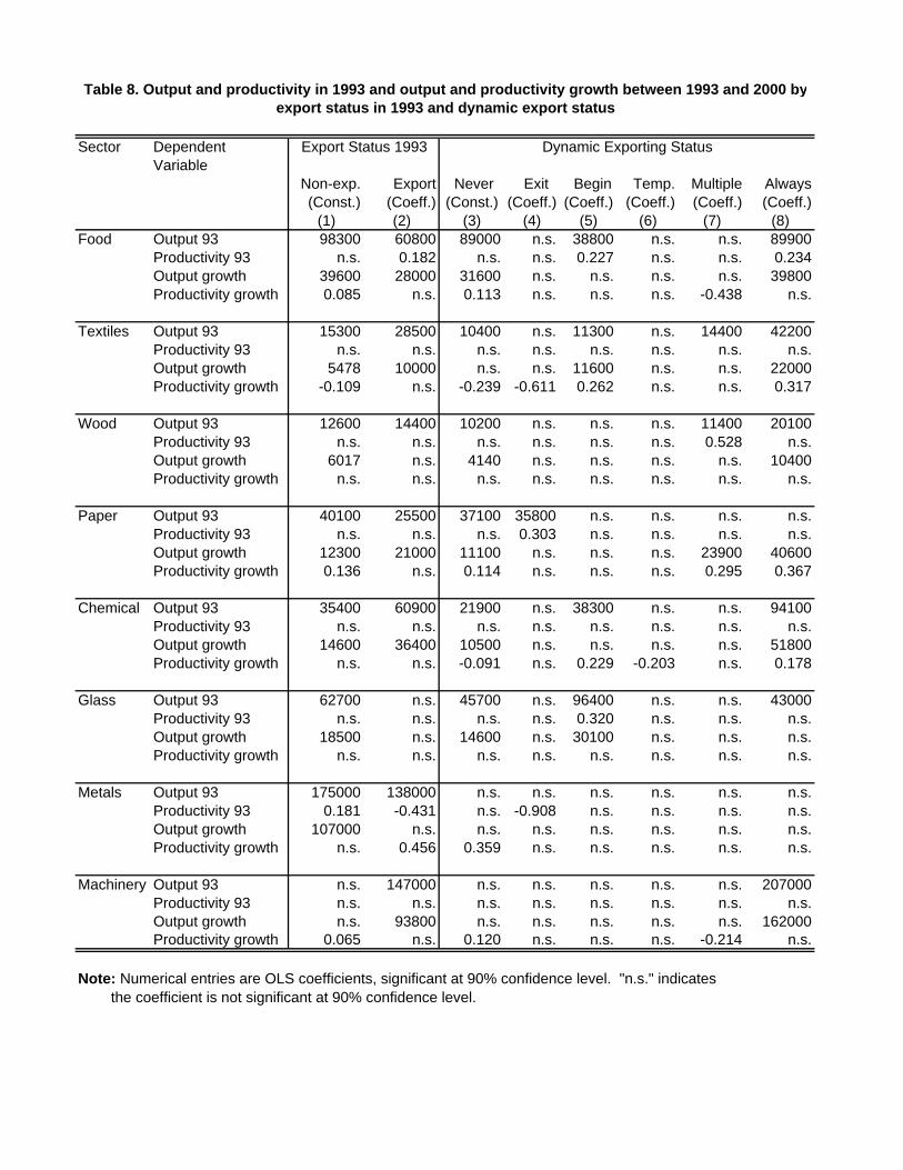
Sector DependentVariable

Non-exp. Export Never Exit Begin Temp. Multiple Always(Const.) (Coeff.) (Const.) (Coeff.) (Coeff.) (Coeff.) (Coeff.) (Coeff.)

(1) (2) (3) (4) (5) (6) (7) (8)Food Output 93 98300 60800 89000 n.s. 38800 n.s. n.s. 89900

Productivity 93 n.s. 0.182 n.s. n.s. 0.227 n.s. n.s. 0.234Output growth 39600 28000 31600 n.s. n.s. n.s. n.s. 39800Productivity growth 0.085 n.s. 0.113 n.s. n.s. n.s. -0.438 n.s.

Textiles Output 93 15300 28500 10400 n.s. 11300 n.s. 14400 42200Productivity 93 n.s. n.s. n.s. n.s. n.s. n.s. n.s. n.s.Output growth 5478 10000 n.s. n.s. 11600 n.s. n.s. 22000Productivity growth -0.109 n.s. -0.239 -0.611 0.262 n.s. n.s. 0.317

Wood Output 93 12600 14400 10200 n.s. n.s. n.s. 11400 20100Productivity 93 n.s. n.s. n.s. n.s. n.s. n.s. 0.528 n.s.Output growth 6017 n.s. 4140 n.s. n.s. n.s. n.s. 10400Productivity growth n.s. n.s. n.s. n.s. n.s. n.s. n.s. n.s.

Paper Output 93 40100 25500 37100 35800 n.s. n.s. n.s. n.s.Productivity 93 n.s. n.s. n.s. 0.303 n.s. n.s. n.s. n.s.Output growth 12300 21000 11100 n.s. n.s. n.s. 23900 40600Productivity growth 0.136 n.s. 0.114 n.s. n.s. n.s. 0.295 0.367

Chemical Output 93 35400 60900 21900 n.s. 38300 n.s. n.s. 94100Productivity 93 n.s. n.s. n.s. n.s. n.s. n.s. n.s. n.s.Output growth 14600 36400 10500 n.s. n.s. n.s. n.s. 51800Productivity growth n.s. n.s. -0.091 n.s. 0.229 -0.203 n.s. 0.178

Glass Output 93 62700 n.s. 45700 n.s. 96400 n.s. n.s. 43000Productivity 93 n.s. n.s. n.s. n.s. 0.320 n.s. n.s. n.s.Output growth 18500 n.s. 14600 n.s. 30100 n.s. n.s. n.s.Productivity growth n.s. n.s. n.s. n.s. n.s. n.s. n.s. n.s.

Metals Output 93 175000 138000 n.s. n.s. n.s. n.s. n.s. n.s.Productivity 93 0.181 -0.431 n.s. -0.908 n.s. n.s. n.s. n.s.Output growth 107000 n.s. n.s. n.s. n.s. n.s. n.s. n.s.Productivity growth n.s. 0.456 0.359 n.s. n.s. n.s. n.s. n.s.

Machinery Output 93 n.s. 147000 n.s. n.s. n.s. n.s. n.s. 207000Productivity 93 n.s. n.s. n.s. n.s. n.s. n.s. n.s. n.s.Output growth n.s. 93800 n.s. n.s. n.s. n.s. n.s. 162000Productivity growth 0.065 n.s. 0.120 n.s. n.s. n.s. -0.214 n.s.

Note: Numerical entries are OLS coefficients, significant at 90% confidence level. "n.s." indicates the coefficient is not significant at 90% confidence level.

Export Status 1993 Dynamic Exporting Status

Table 8. Output and productivity in 1993 and output and productivity growth between 1993 and 2000 byexport status in 1993 and dynamic export status

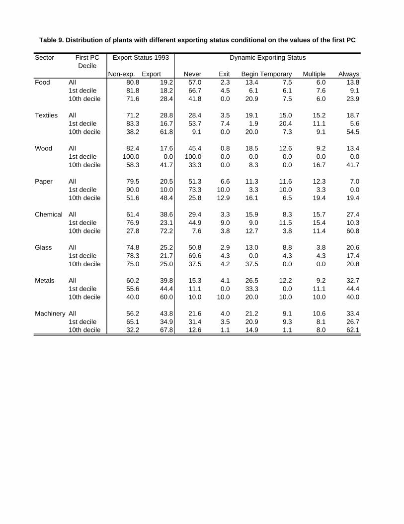
Sector First PCDecile

Non-exp. Export Never Exit Begin Temporary Multiple AlwaysFood All 80.8 19.2 57.0 2.3 13.4 7.5 6.0 13.8

1st decile 81.8 18.2 66.7 4.5 6.1 6.1 7.6 9.110th decile 71.6 28.4 41.8 0.0 20.9 7.5 6.0 23.9

Textiles All 71.2 28.8 28.4 3.5 19.1 15.0 15.2 18.71st decile 83.3 16.7 53.7 7.4 1.9 20.4 11.1 5.610th decile 38.2 61.8 9.1 0.0 20.0 7.3 9.1 54.5

Wood All 82.4 17.6 45.4 0.8 18.5 12.6 9.2 13.41st decile 100.0 0.0 100.0 0.0 0.0 0.0 0.0 0.010th decile 58.3 41.7 33.3 0.0 8.3 0.0 16.7 41.7

Paper All 79.5 20.5 51.3 6.6 11.3 11.6 12.3 7.01st decile 90.0 10.0 73.3 10.0 3.3 10.0 3.3 0.010th decile 51.6 48.4 25.8 12.9 16.1 6.5 19.4 19.4

Chemical All 61.4 38.6 29.4 3.3 15.9 8.3 15.7 27.41st decile 76.9 23.1 44.9 9.0 9.0 11.5 15.4 10.310th decile 27.8 72.2 7.6 3.8 12.7 3.8 11.4 60.8

Glass All 74.8 25.2 50.8 2.9 13.0 8.8 3.8 20.61st decile 78.3 21.7 69.6 4.3 0.0 4.3 4.3 17.410th decile 75.0 25.0 37.5 4.2 37.5 0.0 0.0 20.8

Metals All 60.2 39.8 15.3 4.1 26.5 12.2 9.2 32.71st decile 55.6 44.4 11.1 0.0 33.3 0.0 11.1 44.410th decile 40.0 60.0 10.0 10.0 20.0 10.0 10.0 40.0

Machinery All 56.2 43.8 21.6 4.0 21.2 9.1 10.6 33.41st decile 65.1 34.9 31.4 3.5 20.9 9.3 8.1 26.710th decile 32.2 67.8 12.6 1.1 14.9 1.1 8.0 62.1

Export Status 1993 Dynamic Exporting Status

Table 9. Distribution of plants with different exporting status conditional on the values of the first PC

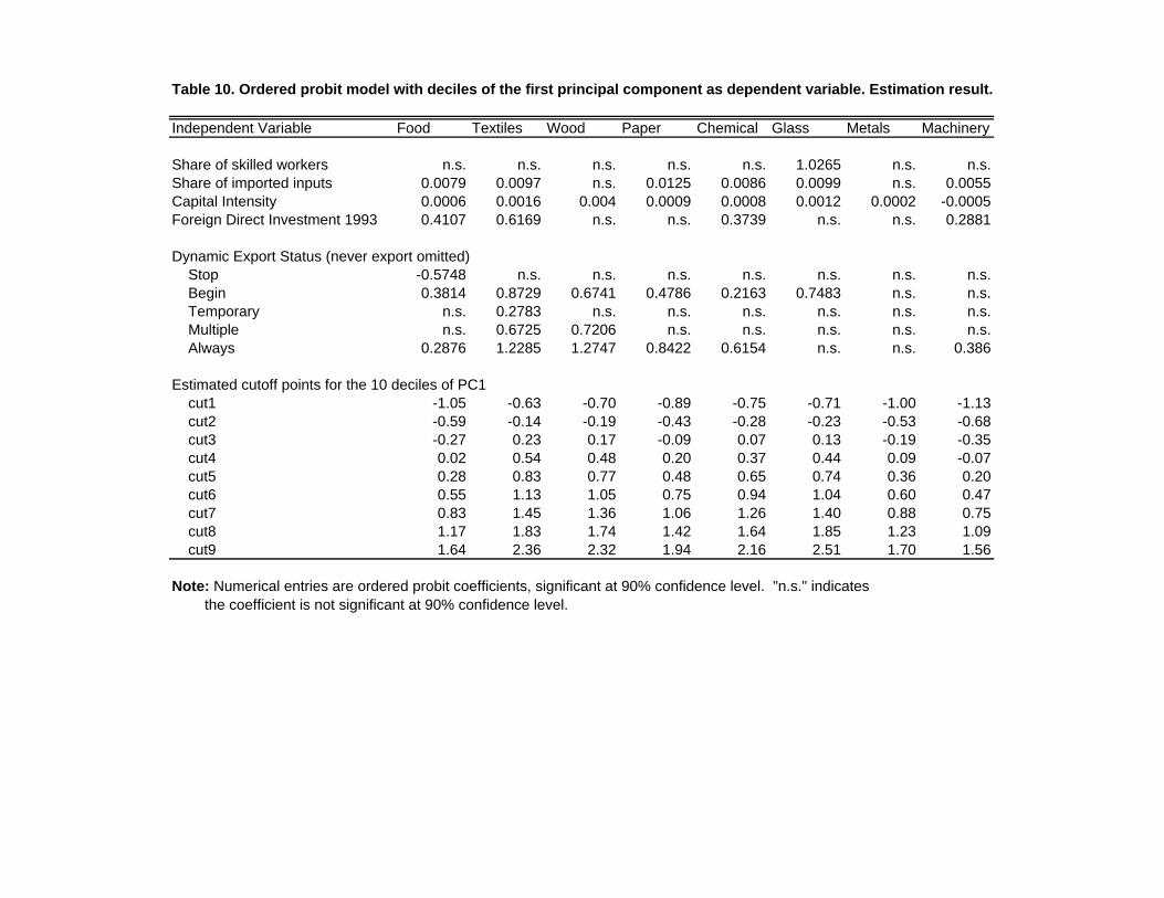
Independent Variable Food Textiles Wood Paper Chemical Glass Metals Machinery

Share of skilled workers n.s. n.s. n.s. n.s. n.s. 1.0265 n.s. n.s.Share of imported inputs 0.0079 0.0097 n.s. 0.0125 0.0086 0.0099 n.s. 0.0055Capital Intensity 0.0006 0.0016 0.004 0.0009 0.0008 0.0012 0.0002 -0.0005Foreign Direct Investment 1993 0.4107 0.6169 n.s. n.s. 0.3739 n.s. n.s. 0.2881

Dynamic Export Status (never export omitted) Stop -0.5748 n.s. n.s. n.s. n.s. n.s. n.s. n.s. Begin 0.3814 0.8729 0.6741 0.4786 0.2163 0.7483 n.s. n.s. Temporary n.s. 0.2783 n.s. n.s. n.s. n.s. n.s. n.s. Multiple n.s. 0.6725 0.7206 n.s. n.s. n.s. n.s. n.s. Always 0.2876 1.2285 1.2747 0.8422 0.6154 n.s. n.s. 0.386

Estimated cutoff points for the 10 deciles of PC1 cut1 -1.05 -0.63 -0.70 -0.89 -0.75 -0.71 -1.00 -1.13 cut2 -0.59 -0.14 -0.19 -0.43 -0.28 -0.23 -0.53 -0.68 cut3 -0.27 0.23 0.17 -0.09 0.07 0.13 -0.19 -0.35 cut4 0.02 0.54 0.48 0.20 0.37 0.44 0.09 -0.07 cut5 0.28 0.83 0.77 0.48 0.65 0.74 0.36 0.20 cut6 0.55 1.13 1.05 0.75 0.94 1.04 0.60 0.47 cut7 0.83 1.45 1.36 1.06 1.26 1.40 0.88 0.75 cut8 1.17 1.83 1.74 1.42 1.64 1.85 1.23 1.09 cut9 1.64 2.36 2.32 1.94 2.16 2.51 1.70 1.56

Note: Numerical entries are ordered probit coefficients, significant at 90% confidence level. "n.s." indicates the coefficient is not significant at 90% confidence level.

Table 10. Ordered probit model with deciles of the first principal component as dependent variable. Estimation result.

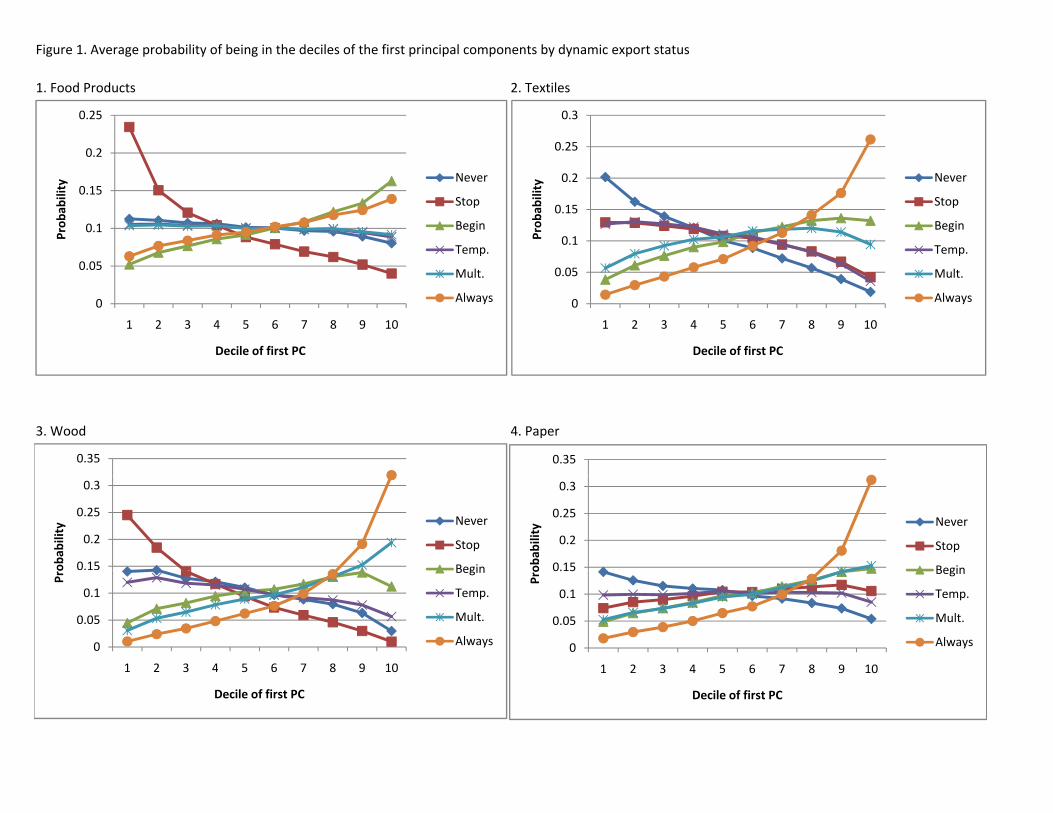
Figure 1. Average probability of being in the deciles of the first principal components by dynamic export status

1. Food Products 2. Textiles

0 15

0.2

0.25

ty

Never 0.2

0.25

0.3

ty

Never

0.05

0.1

0.15

Prob

abili Stop

Begin

Temp.

Mult. 0.05

0.1

0.15

Prob

abili Stop

Begin

Temp.

Mult.

0

1 2 3 4 5 6 7 8 9 10

Decile of first PC

Always 0

1 2 3 4 5 6 7 8 9 10

Decile of first PC

Always

3. Wood 4. Paper

0.35 0.35

0.15

0.2

0.25

0.3

obab

ility

Never

Stop

Begin 0.15

0.2

0.25

0.3

obab

ility

Never

Stop

Begin

0

0.05

0.1

1 2 3 4 5 6 7 8 9 10

Pro Begin

Temp.

Mult.

Always 0

0.05

0.1

0.15

1 2 3 4 5 6 7 8 9 10

Pro Begin

Temp.

Mult.

Always

1 2 3 4 5 6 7 8 9 10

Decile of first PC

1 2 3 4 5 6 7 8 9 10

Decile of first PC

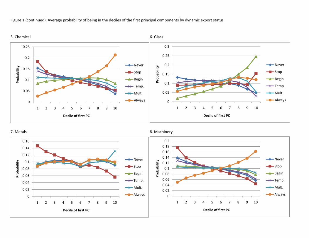
Figure 1 (continued). Average probability of being in the deciles of the first principal components by dynamic export status

5. Chemical 6. Glass

0 25

0.30.25

0 1

0.15

0.2

0.25

Prob

ability

Never

Stop

Begin0.1

0.15

0.2

Prob

ability

Never

Stop

Begin

0

0.05

0.1

1 2 3 4 5 6 7 8 9 10

Temp.

Mult.

Always0

0.05

1 2 3 4 5 6 7 8 9 10

Temp.

Mult.

Always

7. Metals 8. Machinery

Decile of first PCDecile of first PC

0.120.140.160.180.2

bility Never

Stop0.1

0.12

0.14

0.16

bility Never

Stop

00.020.040.060.080.1

Prob

ab

Stop

Begin

Temp.

Mult.

Always0.02

0.04

0.06

0.08

Prob

ab

Stop

Begin

Temp.

Mult.

Always 0

1 2 3 4 5 6 7 8 9 10

Decile of first PC

Always0

1 2 3 4 5 6 7 8 9 10

Decile of first PC

Always