The Monte Carlo method

1

The Monte Carlo method

2

(0,0)

(1,1)

(-1,-1)

(-1,1)

(1,-1)

1Z=

1 If X2+Y210 o/w

• (X,Y) is a point chosen uniformly at random in a 22 square centered at the origin (0,0).

• P(Z=1)=/4.

3

Assume we run this experiment m times, with Zi being the value of Z at the ith run.

If W=iZi, then

W’=4W/m is an estimate of .

.4

][][][11

mZEZEWE

m

ii

m

ii

4

m

W

4

By Chernoff bound,

Def: A randomized algorithm gives an (,)-approximation for the value V if the output X of the algorithm satisfies Pr[|X-V|V] 1-.

.2

]][|][Pr[|

]4

|4

Pr[|]|'Pr[|

12/2

me

WEWEW

mmWW

5

The above method for estimating gives an (,)-approximation, as long as <1 and m large enough.

.)/2(12

22

12/2

ln

me m

6

Thm1: Let X1,…,Xm be independent and identically distributed indicator random variables, with =E[Xi]. If m (3ln(2/))/2, then

I.e. m samples provide an (,)-approximation for .

Pf: Exercise!

.]|1

Pr[|1

m

iiXm

7

Def: FPRAS: fully polynomial randomized approximation scheme.

A FPRAS for a problem is a randomized algorithm for which, given an input x and any parameters and with 0<,<1, the algorithm outputs an (,)-approximation to V(x) in time poly(1/,ln-1,|x|).

8

Def: DNF counting problem: counting the number of satisfying assignments of a Boolean formula in disjunctive normal form (DNF).

Def: a DNF formula is a disjunction of clauses C1C2… Ct, where each clause is a conjunction of literals.

Eg. (x1x2x3)(x2x4)(x1x3x4)

9

Counting the number of satisfying assignments of a DNF formula is actually #P-complete.

Counting the number of Hamiltonian cycles in a graph and counting the number of perfect matching in a bipartite graph are examples of #P-complete problems.

10

A naïve algorithm for DNF counting problem: Input: A DNF formula F with n variables.Output: Y = an approximation of c(F)

The number of satisfying Assigments of F.

1. X0.2. For k=1 to m, do: (a) Generate a random assignment for the n variables, chosen uniformly at random. (b) If the random assignment satisfies F, then X X+1.3. Return Y (X/m)2n.

11

Analysis

Pr[Xk=1]=c(F)/2n.

Let X= and then E[X]=mc(F)/2n.

Xk=1 If the k-th iteration in the algorithm generated a satisfying assignment;0 o/w.

m

kkX

1

).(2][

][ Fcm

XEYE

n

12

Analysis By Theorem 1, X/m gives an (,)-approxi

mation of c(F)/2n, and hence Y gives an (,)-approximation of c(F), when m 32nln(2/))/2c(F).

If c(F) 2n/poly(n), then this is not too bad, m is a poly.

But, if c(F)=poly(n), then m=O(2n/c(F))!

13

Analysis

Note that if Ci has li literals then there are exactly 2n-li satisfying assignments for Ci.

Let SCi denote the set of assignments that satisfy clause i.

U={(i,a): 1it and aSCi}. |U|= Want to estimate Define S={(i,a): 1it and aSCi, aSCj for j<i}.

t

i

nt

ii

iSC11

2|| l

.||)(1t

iiSCFc

14

DNF counting algorithm II: Input: A DNF formula F with n variables. Output: Y: an approximation of c(F).1. X0.2. For k=1 to m do: (a) With probability choose, uniformly at random an assignment aSCi. (b) If a is not in any SCj, j<i, then XX+1.3. Return Y

t

iii SCSC

1

||||

.||)/(1

t

iiSCmX

15

DNF counting algorithm II: Note that |U|t|S|. Why? Let Pr[i is chosen]=

Then Pr[(i,a) is chosen] =Pr[i is chosen]Pr[a is chosen|i is chosen] =

||||||||1

USCSCSC i

t

iii

.||

1

||

1

||

||

USCU

SC

i

i

16

DNF counting algorithm II: Thm: DNF counting algorithm II is an FPRAS f

or DNF counting problem when m=(3t/2)ln(2/).

Pf: Step 2(a) chooses an element of U uniformly at random.

The probability that this element belongs to S is at least 1/t.

Fix any ,>0, and let m= (3t/2)ln(2/).poly(t,1/,ln(1/))

17

DNF counting algorithm II: The processing time of each sample is poly(t).

By Thm1, with m samples, X/m gives an (,)-approximation of c(F)/|U| and hence Y gives an (,)-approximation of c(F).

18

Counting with Approximate Sampling

Def: w: the output of a sampling algorithm for a finite sample space .

The sampling algorithm generates an -uniform sample of if, for any subset S of , |Pr[wS]-|S|/|||.

19

Def: A sampling algorithm is a fully polynomial almost uniform sampler (FPAUS) for a problem if, given an input x and >0, it generates an -uniform sample of (x) in time poly(|x|,ln(1/)).

Consider an FPAUS for independent sets would take as input a graph G=(V,E) and a parameter .

The sample space: the set of all independent sets in G.

20

Goal: Given an FPAUS for independent sets, we construct an FPRAS for counting the number of independent sets.

Assume G has m edges, and let e1,…,em be an arbitrary ordering of the edges.

Ei: the set of the first i edges in E and let Gi=(V,Ei).

(Gi): denote the set of independent sets in Gi.

21

|(G0)|=2n. Why?

To estimate |(G)|, we need good estimates for

.|)(||)(|

|)(|

|)(|

|)(|

|)(|

|)(||)(| 0

0

1

2

1

1

GG

G

G

G

G

GG

m

m

m

m

.,..,1,|)(|

|)(|

1

miG

Gr

i

ii

22

Let be estimate for ri, then

To evaluate the error, we need to bound the ratio

To have an (,)-approximation, we want Pr[|R-1|]1-.

ir~ .~2|~)(|

1

m

ii

n rG

.~

1

m

i i

i

r

rR

23

Lemma: Suppose that for all i, 1im, is an (/2m,/m)-approximation for ri. Then Pr[|R-1|]1-.

Pf: For each 1im, we have

ir~

.1]2

|~Pr[|m

rm

rr iii

24

Equivalently,

.]2

|~Pr[|m

rm

rr iii

.]2

|~|,Pr[ iii r

mrri

.1]2

|~|,Pr[ iii r

mrri

.1]2

1~

21,Pr[

mr

r

mi

i

i

.1])2

1(~

)2

1Pr[(1

mm

i i

im

mr

r

m

.1]11Pr[ R

25

Estimating ri: Input: Graph Gi-1=(V,Ei-1) and Gi=(V,Ei) Output: = an approximation of ri.1. X02. Repeat for M=(1296m2/2)ln(2m/) independent trials: (a) Generate an (/6m)-uniform sample from (Gi-1). (b) If the sample is an independent set in Gi, then XX+1.3. Return X/M.

ir~

ir~

26

Lemma: When m1 and 0<1, the procedure for estimating ri yields an (/2m,/m)-approximation for ri.

Pf: Suppose Gi-1 and Gi differ in that edge {u,v} is i

n Gi but not in Gi-1. (Gi) (Gi-1). An independent set in (Gi-1)\(Gi) contains b

oth u and v.

27

Associate each I(Gi-1)\(Gi) with an independent set I\{v}(Gi).

Note that I’(Gi) is associated with no more than one independent set I’{v}(Gi-1)\(Gi), thus |(Gi-1)\(Gi)| |(Gi)|.

It follows that.2

1

|)(\)(||)(|

|)(|

|)(|

|)(|

11

iii

i

i

ii GGG

G

G

Gr

28

Let Xk=1 if the k-th sample is in (Gi) and 0 o/w. Because our samples are generated by an (/6

m)-uniform sampler, by definition,.

6|)(|

|)(|]1Pr[

1 mG

GX

i

ik

.6|)(|

|)(|][

1 mG

GXE

i

ik

29

By linearity of expectations,

.6|)(|

|)(|][

1

1

mG

G

M

XE

i

i

M

kk

.6|)(|

|)(|][|]~[|

1

1

mG

G

M

XErrE

i

i

M

kk

ii

Since ri1/2, we have

.3

1

62

1

6]~[

mmrrE ii

30

If M3ln(2m/)/(/12m)2(1/3)=1296m2-

2ln(2m/), then

Equivalently, with probability 1- /m,

.]~[12

]~[~Pr12

1]~[

~Pr

mrE

mrEr

mrE

riii

i

i

.12

1]~[

~

121

mrE

r

m i

i -----(1)

31

As we have

Using, ri1/2, then

.6

1]~[

61

ii

i

i mrr

rE

mr

-----(2)

,6

|]~[|m

rrE ii

.3

1]~[

31

mr

rE

m i

i

32

Combining (1) and (2), with probability 1-/m,

This gives the desired (/2m,/m)-approximation.

Thm: Given FPAUS for independent sets in any graph, we can construct an FPRAS for the number of independent sets in a graph G.

.2

1)12

1)(3

1(~

)12

1)(3

1(2

1mmmr

r

mmm i

i

33

The Markov Chain Monte Carlo Method

The Markov Chain Monte Carlo Method provides a very general approach to sampling from a desired probability distribution.

Basic idea: Define an ergodic Markov chain whose set of states is the sample space and whose stationary distribution is the required sampling distribution.

34

Lemma: For a finite state space and neighborhood structure {N(x)|x}, let N=maxx|N(x)|.

Let M be any number such that MN. Consider a Markov chain where

If this chain is irreducible and aperiodic, then the stationary distribution is the uniform distribution.

Px,y=1/M if xy and yN(x)0 if xy and yN(x)1-N(x)/M if x=y.

35

Pf: For xy, if x=y, then xPx,y=yPy,x, since Px,y=Py,x

=1/M.

It follows that the uniform distribution x=1/|| is the stationary distribution by the following theorem.

36

Thm: P: transition matrix of a finite irreducible and e

rgodic Markov chain. If there are nonnegative numbers =(0,..,n) such that and if, for any pair of states i,j, iPi,j=jPj,i, then

is the stationary distribution corresponding to P.

Pf: Since , it follows that is the unique stat

ionary distribution of the Markov Chain.

10

n

ii

.0

,0

, j

n

iijj

n

ijii PP

. P

10

n

ii

37

Eg. Markov chain with states from independent sets in G=(V,E).

1. X0 is an arbitrary independent set in G.2. To compute Xi+1: (a) choose a vertex v uniformly at random from V; (b) if vXi then Xi+1=Xi\{v}; (c) if vXi and if adding v to Xi still gives an independent set, then Xi+1=Xi{v}; (d) o/w, Xi+1=Xi.

38

The neighbors of a state Xi are independent sets that differ from Xi in just one vertex.

Since every state is reachable from the empty set, the chain is irreducible.

Assume G has at least one edge (u,v), then the state {v} has a self-loop (Pv,v>0), thus aperiodic.

When xy, it follows that Px,y=1/|V| or 0, by the previous lemma, the stationary distribution is the uniform distribution.

39

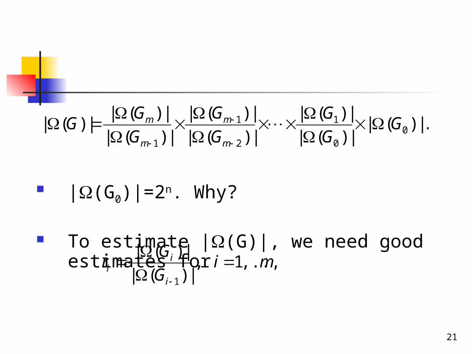
The Metropolis Algorithm(When stationary distribution is nonuniform)

Lemma: For a finite state space and neighborhood structure {N(x)|x}, let N=maxx|N(x)|.

Let M be and number such that MN. For all x, let x>0 be the desired probability of state x in the stationary distribution. Consider a Markov chain

Then, if this chain is irreducible and aperiodic, then the stationary distribution is given by x.

Px,y=(1/M)min(1,y/x) if xy and yN(x)0 if xy and yN(x)1-yxPx,y if x=y.

40

Pf: For any xy, if xy, then Px,y=1/M and Py,x=(1/

M)(x/y). It follows that Px,y=1/M=(y/x)Py,x. xPx,y=yPy,x.

Similarly, for x>y. Again, by the previous theorem, x’s form the

stationary distribution.

41

Eg. Create a Markov chain, in the stationary distribution, each independent set I has probability proportional to |I|, for some >0.

I.e. x=|Ix|/B, where Ix is the independent set corresponding to state x and B=x|Ix|.

Note that, when =1, this is the uniform distribution.

42

1. X0 is an arbitrary independent set in G.2. To compute Xi+1: (a) choose v uniformly at random from V; (b) if vXi then Xi+1=Xi\{v} with probability min(1,1/); (c) if vXi and Xi{v} still gives an independent set, then put Xi+1=Xi{v} with probability min(1,); (d) o/w, set Xi+1=Xi.