The Möbius Framework and Its Implementation

1

The Mobius Framework and Its ImplementationDaniel D. Deavours, Graham Clark, Tod Courtney, David Daly, Salem Derisavi, Jay M. Doyle,

William H. Sanders, and Patrick G. Webster

Abstract— The Mobius framework is an environment forsupporting multiple modeling formalisms and solution tech-niques. Models expressed in formalisms that are compati-ble with the framework are translated into equivalent mod-els using Mobius framework components. This translationpreserves the structure of the models, allowing efficient so-lutions. The framework is implemented in the tool by awell-defined abstract functional interface. Models and solu-tion techniques interact with one another through the useof the standard interface, allowing them to interact withMobius framework components, not formalism components.This permits novel combinations of modeling techniques,and will be a catalyst for new research in modeling tech-niques. This paper describes our approach, focusing on the“atomic model.” We describe the formal description of theMobius components as well as their implementations in oursoftware tool.

Keywords—Stochastic models, modeling formalisms, mod-eling frameworks, modeling tools, Markov models, stochas-tic Petri nets, PEPA, execution policy.

I. Introduction

Performance and dependability modeling is an integralpart of the design process of many computer and commu-nication systems. A variety of techniques have been devel-oped to address different issues of modeling. For example,combinatorial models were developed to assess reliabilityand availability under strong independence assumptions;queuing networks were developed to assess system perfor-mance; and Markov process-based approaches have becomepopular for evaluating performance with synchronization ordependability without independence assumptions. Finally,simulation has been used extensively when other methodsfail.

As techniques for solving models advanced, formalisms(or formal languages for expressing models) were also de-veloped. Each formalism has its own merits. Some for-malisms afford very efficient solution methods; for exam-

D. D. Deavours is with the Information and TelecommunicationTechnology Center, University of Kansas at Lawrence. Email: [email protected]

G. Clark is a Software Engineer with Citrix Systems, Inc. Email:[email protected]

T. Courtney, D. Daly, S. Derisavi, and W. H. Sanders are withthe Center for Reliable and High-Performance Computing, Univer-sity of Illinois at Urbana-Champaign. Email: {tod, ddaly, derisavi,whs}@crhc.uiuc.edu

J. M. Doyle is a Software Engineer with Honeywell in Fort Wash-ington, PA. Email: [email protected]

P. G. Webster is a Design Engineer at ARM, Inc. in Austin, TX.Email: [email protected]

This material is based upon work supported in part by the NationalScience Foundation under Grant No. 9975019 and by the MotorolaCenter for High-Availability System Validation at the University ofIllinois (under the umbrella of the Motorola Communications Cen-ter). Any opinions, findings, and conclusions or recommendationsexpressed in this material are those of the authors and do not neces-sarily reflect the views of the NSF or Motorola.

ple, BCMP [1] queuing networks admit product-form solu-tions, while superposed generalized stochastic Petri nets(SGSPNs) [2] afford Kronecker-based solution methods,and colored GSPNs (CGSPNs) [3] yield state-space reduc-tions. Other formalisms, such as SPNs [4] and SPAs [5],provide a simple elegance in their modeling primitives,while a number of extensions, such as stochastic activitynetworks (SANs) [6], were developed for compactly express-ing complex behaviors.

Along with formalisms, tools have been developed. Atool is generally built around a single formalism and one ormore solution techniques, with simulation sometimes avail-able as a second solution method. [7] lists a number ofsuch tools, such as DyQN-Tool+ [8], which uses dynamicqueuing networks as its high-level formalism; GreatSPN[9], which is based on GSPNs [10]; UltraSAN [11], which isbased on SANs [6]; SPNP [12], which is based on stochas-tic reward networks [13]; and TANGRAM-II [14], whichis an object- and message-based formalism for evaluatingcomputer and communication systems. While all of thesetools are useful within the domains for which they wereintended, they are limited in that all parts of a model mustbe built in the single formalism that is supported by thetool. Thus, it is difficult to model systems that cross dif-ferent domains and would benefit from multiple modelingtechniques.

A. Related Work

We will now briefly review the tools that are most closelyrelated to Mobius; a more complete discussion of relatedwork can be found in [7].

One approach has been what we call the “integrated soft-ware environment” approach. This approach seeks to unifyseveral different modeling tools of the kind described aboveinto a single software environment. Examples are IMSE(Integrated Modeling Support Environment) [15], IDEAS(Integrated Design Environment for Assessment of Com-puter Systems and Communication Networks) [16], andFreud [17]. One problem with these approaches is thatsince they use existing tools, the degree to which for-malisms and solution methods of different tools may in-teract is limited.

A more aggressive approach is the “multi-formalismmulti-solution” approach, in which a tool implements morethan one formalism and solution technique. Models ex-pressed in different formalisms may interact by passing re-sults from one model to another. The earliest attemptto do this, to the best of our knowledge, was the combi-nation of multiple modeling formalisms in SHARPE [18].In the SHARPE modeling framework, models can be ex-pressed as combinatorial reliability models, directed acyclic

2

task precedence graphs, Markov and semi-Markov models,product-form queuing networks, or GSPNs. Interactionsbetween formalisms are limited to the exchange of results,either as single numbers or as exponential-polynomial prob-ability distribution functions. Another tool that integratesmultiple modeling formalisms in a single software environ-ment is SMART [19]. SMART supports the analysis ofmodels expressed as SPNs and queuing networks, and thetool is implemented in a way that permits the easy inte-gration of new solution algorithms. The DEDS (DiscreteEvent Dynamic System) toolbox [20] also integrates mul-tiple modeling formalisms into a single software environ-ment, but does so by converting models expressed in dif-ferent modeling formalisms into a common “abstract Petrinet notation.” Once expressed in this abstract formalism,models may be solved using a variety of functional andquantitative analysis approaches for Markovian models.

B. The Mobius Approach

We take an integrated multi-formalism multi-solutionapproach with Mobius [7]. Our goal is to build a tool inwhich each model formalism or solver is, to the extent pos-sible, modular, in order to maximize potential interaction.A modular modeling tool is possible because many oper-ations on models, such as composition (described later),state-space generation, and simulation are largely indepen-dent of the formalism being used to express the model.

This approach has several advantages. First, it allowsfor novel combinations of modeling techniques. For ex-ample, to the best of our knowledge, the Replicate/Joinmodel composition approach of [21] has been used exclu-sively with SANs. This exclusivity is artificial, and in theMobius tool, Replicate/Join can be used with virtually anyformalism that can produce a labelled transition system,such as PEPA [22].

Another advantage is the ease with which new ap-proaches may be integrated into the tool. Perhaps the mostconvincing argument for this comes from our own experi-ence. To the extent possible, we have incorporated newresearch results into our successful modeling tool, Ultra-SAN. For a number of practical reasons, many of our recentresearch results have only been developed into prototypes(for example, as described in [23–27]), and are not gener-ally available to other users. In particular, we would haveliked to develop a new composition formalism called “graphcomposition” [27], but found that it would have been dif-ficult to include it in UltraSAN because of the inherentlyclosed nature of the software design. Mobius has been de-signed to include these prototyped modeling techniques, aswell as to be extensible to include future techniques.

The ability to add new components simply would bene-fit researchers and users alike. Researchers would be ableto add a new component to the tool and expect it to beable to interact immediately with other components. Theywould also be able to compare competing techniques di-rectly. Additionally, researchers would have access to thework of others, and be able to extend and compare tech-niques. Users would benefit by having access to the most

recent developments in conjunction with previously exist-ing techniques. They would also benefit from having amodular, “toolbox” approach that would allow them tochoose the most appropriate tool or tools for the job.

While we would like Mobius to have a great deal of flex-ibility, we would also like to be able to retain the ability toperform efficient solution. Efficient solution is usually pos-sible because of some special structure or condition that ismet in the model, and Mobius should preserve such fea-tures.

For all of the above reasons, we argue that an open,multi-formalism, multi-solution modeling framework wouldrepresent a significant step forward in advancing the state-of-the-art in performance/dependability modeling tech-niques. Such a framework would maximize potential inter-action of techniques, while maintaining the independence ofthose techniques. This would require the creation of a suffi-ciently general and abstract representation of a model thatalso retained the ability to be solved efficiently. Mobius isour attempt at a multi-formalism, multi-solution modelingframework for discrete event stochastic systems. Mobiusshould support existing formalisms as well as formalisms tobe developed in the future. Therefore, we make no claim orproof that ours is the best or only solution, but instead of-fer several examples supporting the claim that it is a goodsolution.

In this paper, we present an overview of the Mobiusframework and tool, and describe the “atomic model” andits implementation issues in greater detail. The paper isintended to give a view of the issues involved in developingthe tool and in implementing new formalisms.

II. Mobius Overview

The Mobius framework is an environment for support-ing multiple modeling formalisms. In order for a formalismto be compatible with the framework, the formalism mustbe able to translate any formalism model into an equiva-lent model that uses Mobius framework components. Sincemodels are constructed in the specific formalisms, the ex-pressive advantages of the particular formalisms are pre-served. Because all models are transformed into frame-work components, all models and solution techniques inthe framework are able to interact with each other. Theframework is also extensible, allowing new formalisms andsolvers to be added with little impact on existing ones, sincenew formalisms and solvers communicate using frameworkcomponents.

In order to accomplish the desired goal of extensibil-ity, framework components must be general enough to ex-press a variety of different formalism components. How-ever, there is a subtle but important point concerning theMobius framework: it is not meant to be a universal for-malism. While formalisms may express only a subset ofwhat is possible within the framework, we believe that thesubsets expressed by formalisms are carefully chosen byexperienced researchers to accomplish various purposes.

3

RewardVariables

PropertiesState

VariablesActions

Results

AtomicModel

Model

ComposedModel

Solved

ModelConnected

ModelComposition

SolverExecution Policy

ModelModel Connection

Reward

Möbius

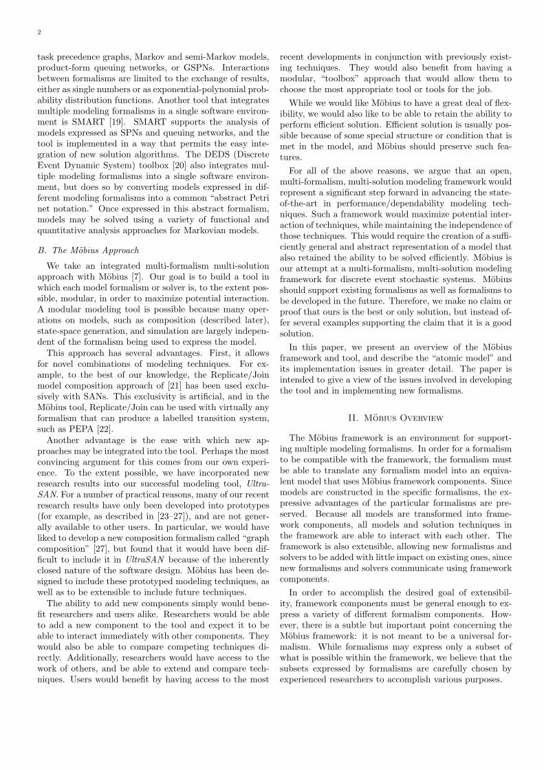
Fig. 1. Mobius framework components.

A. Framework components

In order to define the framework, we must identify andabstract the common concepts found in most formalisms.We also must generalize the process of building and catego-rizing models. We divide the model construction processinto several steps. Each step in the process generates anew type of model. The illustration shown in Figure 1highlights the various model types and other componentswithin the Mobius framework.

The first step in the model construction process is togenerate a model using some formalism. This most basicmodel in the framework is called an atomic model, and ismade up of state variables, actions, and properties. Statevariables (for example, places in the various stochastic ex-tensions to Petri nets, or queues in queuing networks) holdstate information about a model, while actions (such astransitions in SPNs or servers in queuing networks) are themechanism for changing model state. Properties provideinformation about a model that may be needed to allowuse of a specialized solver, or to make the solution processmore efficient for some solvers.

After an atomic model is created, frequently the nextstep is to specify some measures of interest on the modelusing some reward specification formalism, e.g., [28]. TheMobius framework captures this pattern by having a sep-arate model type, called reward models, that augmentsatomic models with reward variables. Some formalismsmay have the measure specification as part of the formal-ism description. In that case, the formalism produces areward model instead of an atomic model.

If the model being constructed is intended to be part of alarger model, then the next step is to compose it with othermodels to form a larger model. This is sometimes used as aconvenient technique to make the model modular and eas-ier to construct; at other times, the ways that models arecomposed can lead to efficiencies in the solution process.Examples include the Replicate/Join composition formal-ism [21] and the graph composition formalism of [27], in

which symmetries may be detected and state lumping maybe performed. Another notable composed model techniqueis synchronization on actions, which is found, for example,in stochastic process algebras (SPAs) such as PEPA [5], aswell as in stochastic automata networks (and also SANs,e.g., [29]) and superposed GSPNs (e.g., [2, 30]). Althougha composed model is a single model with its own statespace, it is not a “flat” model. It is hierarchically builtfrom submodels, which largely preserve their formalism-specific characteristics so the composed model does notdestroy the structural properties of the submodels. Notethat the compositional techniques do not depend on theparticular formalism of the atomic models that are beingcomposed, provided that any necessary requirements aremet. Composition of different formalisms (specifically SANand PEPA) is demonstrated by example models included inthe Mobius distribution. Additionally, we note that rewardvariables can also be added to a composed model.

The next step is typically to apply some solver to com-pute a solution and generate a solved model. We call anymechanism that calculates the solution to reward variablesa solver. The calculation method could be exact, approx-imate, or statistical, and it may take advantage of modelproperties that are due to the atomic model formalisms,model composition, and reward specification. Note thatsolvers operate on framework components, not formalismcomponents. Consequently, a solver may operate on amodel independent of the formalism in which the modelwas constructed, so long as the model has the propertiesnecessary for the solver.

The computed solution to a reward variable is called aresult. Since the reward variable is a random variable, theresult is expressed as some characteristic of a random vari-able. This may be, for example, the mean, variance, ordistribution of the reward variable. The result may alsoinclude any solver-specific information that relates to thesolution, such as any errors, the stopping criterion used, orthe confidence interval. A solution calculated in this waymay be the final desired measure, or it may be an interme-diate step in further computation. If a result is intendedfor further computation, then the result may capture theinteraction between multiple reward models that togetherform a connected model.

A connected model is an ordered set of reward modelsand their corresponding solution methods in which inputparameters to some of the models depend on the results ofother models in the set. This is useful for modeling usingdecompositional approaches, such as that used in [31]. Inthose cases, the model of interest is a set of reward mod-els with dependencies expressed through results, where theoverall model may be solved through a system of nonlinearequations (if a solution exists).

B. Tool description

The Mobius tool is our implementation of the Mobiusframework. It ensures that all formalisms translate modelcomponents into framework components through the use ofthe abstract functional interface (AFI) [32]. The AFI pro-

4

vides the common interface between model formalisms andsolvers that allows formalism-to-formalism and formalism-to-solver interactions. It uses abstract classes to implementMobius framework components. The AFI is built fromthree main base classes: one for state variables, one foractions, and one that defines overall atomic model behav-ior. Each of these classes defines an interface used by theMobius tool when building composed models, specifyingreward variables, and solving models. There are subtle dif-ferences between the current AFI and the framework, pre-dominantly due to delays in the implementation of newerframework concepts (such as properties), and additions tothe AFI to increase efficiency or ease of use of the tool.

The various components of a model formalism must bepresented as classes derived from the Mobius AFI classesin order to be implemented in the Mobius tool. Othermodel formalisms and model solvers in the tool are thenable to interact with the new formalism by accessing itscomponents through the Mobius abstract class interfaces.

The main user interface for the Mobius tool presentsa series of editors that are classified according to modeltype. Each formalism or solver supported by Mobius hasa corresponding editor in the main interface. These edi-tors are used to construct and specify the model, possiblyperforming some formalism-specific analysis and propertydiscovery, and to define the parameters for the solutiontechniques. The tool dynamically loads each formalism-specific editor from a java archive (jar file) at startup.This design allows new formalisms and their editors to beincorporated into the tool without modification or recompi-lation of the existing code, thus supporting the extensibilityof the Mobius tool.

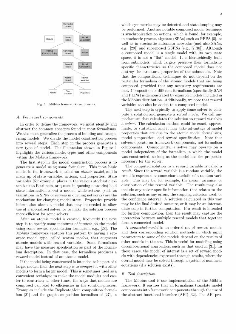
Models can be solved either analytically/numerically orby simulation. From each model, C++ source code is gen-erated and compiled, and the object files are packaged toform a library archive. These libraries are linked togetheralong with the tool’s base libraries to form the executablefor the solver. The executable is run to generate the results.The base libraries implement the components of the partic-ular model formalism, the AFI, and the solver algorithms.The organization of Mobius components to support thismodel construction procedure is shown in Figure 2.

We believe that the majority of modeling techniques canbe supported within the Mobius framework and tool. Bymaking different modeling processes (such as adding mea-sures, composing, solving, and connecting) modular, wecan maximize the amount of interaction allowable betweenthese processes. That approach also makes it possible forthe framework to be extensible, in that new atomic mod-eling formalisms, reward formalisms, compositional for-malisms, solvers, and connection formalisms may be addedindependently. All of these features will be discussed inmore detail in the remaining sections. Special focus will begiven to the atomic model, since it represents a generaliza-tion of multiple modeling formalisms and is one of the maincontributions of Mobius. The key elements of atomic mod-els are state variables and actions; they are the subjects ofthe next two sections.

Code Code

Object

Code

Object

Code

Object

Solver

Libraries

Formalism

Executable

Libraries

Solver

Object

Linker

AtomicModelEditor

Composed

EditorModel

PVEditor Editor

Study

Main Application

Fig. 2. Mobius tool architecture

III. State variables

A state variable typically represents some portion of thestate of a model, and is a basic component of a model. Itcan represent something as simple as the number of jobswaiting in a queue, or as complex as the state of an ATMswitch.

Different formalisms represent state variables differently.For example, SPNs and extensions have places that con-tain tokens, so the set of values that a place can take on isthe set of natural numbers. Colored GSPNs (CGSPNs) [3]have been extended so that tokens can take on a numberof different colors at a place, making the value of a coloredplace a bag or multi-set. Queuing networks with differ-ent customer classes can have more complicated notions ofstate, such as those found in extended queuing networks[33], in which each job (customer) may have an associatedjob variable, which is typically implemented as an array ofreal numbers.

To capture and express all state variable types in existingformalisms in Mobius, we must create a generalized statevariable that can be used to create specific state variables.By using a generalized state variable, we enjoy all the bene-fits of a framework we discussed earlier. Specifically, solversor higher-level model types can interact with Mobius statevariables (in the framework or the tool), instead of withthe variety of different formalism state variables. Finally,any efficiencies that may be gained through any structuralknowledge can be preserved through the use of properties.

A. Components of State Variables

In the Mobius framework, a state variable is made up ofthree primary components: a value, a type, and an initialvalue distribution, which includes a set of possible initialstates. The value of a state variable represents a particu-lar configuration that the modeled component may be in,while the type of a state variable represents the range ofvalues that the variable may take. The initial value distri-bution probabilistically gives the distribution of values at

5

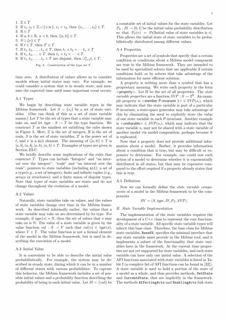
1. Z ∈ T2. If i1, i2 ∈ Z ∪ {±∞}, i1 < i2, then {i1, . . . , i2} ∈ T .3. R ∈ T4. If a, b ∈ R, a < b, then ([a, b)] ∈ T .5. S ∪ {ν} ∈ T6. If t ∈ T , then 2t ∈ T .7. If t1, t2, . . . , tn ∈ T , then t1 × t2 × · · · tn ∈ T8. If t1, t2, . . . ∈ T , then t1 × t2 × · · · ∈ T .9. If t1, t2, . . . , tn ∈ T are disjoint, then ∪ni=1ti ∈ T .

Fig. 3. Construction of the type set T .

time zero. A distribution of values allows us to considermodels whose initial states may vary. For example, wecould consider a system that is in steady state, and mea-sure the expected time until some important event occurs.

A.1 Types

We begin by describing state variable types in theMobius framework. Let S = {si} be a set of state vari-ables. (One can think of this as a set of state variablenames.) Let T be the set of types that a state variable maytake on, and let type : S → T be the type function. Weconstruct T as the smallest set satisfying the rules shownin Figure 3. Here, Z is the set of integers, R is the set ofreals, S is the set of state variables, 2t is the power set oft, and ν is a nil element. The meaning of ([a, b)] ∈ T is[a, b], (a, b], [a, b), (a, b) ∈ T . Examples of types are given inSection III-C.

We briefly describe some implications of the rules thatconstruct T . Types can include “Integers” and “an inter-val over the integers”; “reals” and “an interval over thereals”; pointers to state variables (including nil); a set ofa type(e.g., a set of integers); finite and infinite tuples (e.g.,arrays or structures); and a finite union of disjoint types.Note that types of state variables are static and do notchange throughout the evolution of a model.

A.2 Values

Naturally, state variables take on values, and the valuesof state variables change over time in the Mobius frame-work. As described informally earlier, the values that astate variable may take on are determined by its type. Forexample, if type(s) = N, then the set of values that s maytake on is N. The value of a state variable is given by thevalue function val : S → V such that val(s) ∈ type(s),where V ∈ T . The value function is not a formal elementof the model in the Mobius framework, but is used in de-scribing the execution of a model.

A.3 Initial Value

It is convenient to be able to describe the initial valueprobabilistically. For example, the system may be de-scribed in steady state, during which it can be in a numberof different states with various probabilities. To capturethis behavior, the Mobius framework includes a set of pos-sible initial values and a probability function describing theprobability of being in each initial value. Let IS = {val} be

a countable set of initial values for the state variables. LetPS : IS → [0, 1] be the initial value probability distributionso that PS(v) = Pr[Initial value of state variables is v].This allows the initial state of state variables to be proba-bilistically distributed among different values.

A.4 Properties

Properties are a set of symbols that specify that a certaincondition or conditions about a Mobius model componentare true in the Mobius framework. They are intended tobe used by specialized solvers that are applicable if certainconditions hold, or by solvers that take advantage of theinformation for more efficient solution.

A property is nothing more than a symbol that has aproprietary meaning. We write each property in the form<property>. Let Π be the set of all properties. The statevariable properties are a function SVP : S → 2Π. An exam-ple property is <member P-invariant 1> ∈ SVP(si), whichmay indicate that the state variable is part of a particularP-invariant; a state-space generator may take advantage ofthis by eliminating the need to explicitly store the valueof one state variable in each P-invariant. Another exampleis <unsharable> ∈ SVP(si), which may indicate that thestate variable si may not be shared with a state variable ofanother model via model composition, perhaps because itis replicated.

Note that a property does not provide additional infor-mation about a model. Rather, it provides informationabout a condition that is true, but may be difficult or ex-pensive to determine. For example, one could test eachaction of a model to determine whether it is exponentiallydistributed in all states, but that may be expensive com-pared to the effort required if a property already states thatthis is true.

A.5 Definition

Now we can formally define the state variable compo-nents of a model in the Mobius framework to be the com-ponents

SV = (S, type, IS , PS ,SVP) .

B. State Variable Implementation

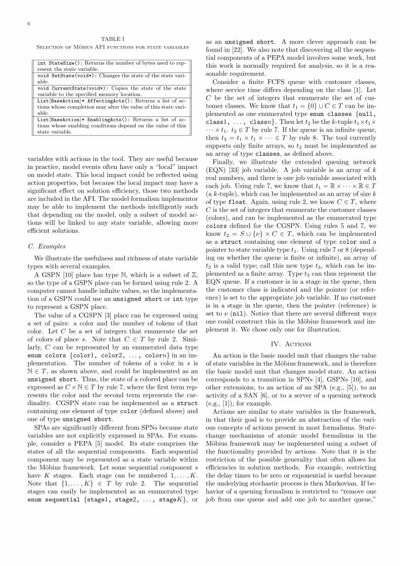
The implementation of the state variables requires thedevelopment of a C++ class to represent the core function-ality of a state variable. All specific state variable types willinherit this base class. Therefore, the base class for Mobiusstate variables, BaseSV, specifies the minimal interface thatany state variable must provide in the Mobius tool, and itimplements a subset of the functionality that state vari-ables have in the framework. At the current time proper-ties are not yet supported for state variables, and each statevariable can have only one initial value. A selection of theAFI functions associated with state variables is listed in Ta-ble I (a complete list of AFI functions can be found in [32]).A state variable is used to hold a portion of the state ofa model as a whole, and thus provides methods, SetStateand CurrentState, that are implicitly in the framework.The methods AffectingActs and EnablingActs link state

6

TABLE I

Selection of Mobius AFI functions for state variables

int StateSize(): Returns the number of bytes used to rep-resent the state variable.void SetState(void*): Changes the state of the state vari-able.void CurrentState(void*): Copies the state of the statevariable to the specified memory location.List〈BaseAction〉* AffectingActs(): Returns a list of ac-tions whose completion may alter the value of this state vari-able.List〈BaseAction〉* EnablingActs(): Returns a list of ac-tions whose enabling conditions depend on the value of thisstate variable.

variables with actions in the tool. They are useful becausein practice, model events often have only a “local” impacton model state. This local impact could be reflected usingaction properties, but because the local impact may have asignificant effect on solution efficiency, those two methodsare included in the AFI. The model formalism implementormay be able to implement the methods intelligently suchthat depending on the model, only a subset of model ac-tions will be linked to any state variable, allowing moreefficient solutions.

C. Examples

We illustrate the usefulness and richness of state variabletypes with several examples.

A GSPN [10] place has type N, which is a subset of Z,so the type of a GSPN place can be formed using rule 2. Acomputer cannot handle infinite values, so the implementa-tion of a GSPN could use an unsigned short or int typeto represent a GSPN place.

The value of a CGSPN [3] place can be expressed usinga set of pairs: a color and the number of tokens of thatcolor. Let C be a set of integers that enumerate the setof colors of place s. Note that C ∈ T by rule 2. Simi-larly, C can be represented by an enumerated data typeenum colors {color1, color2, . . . , colorn} in an im-plementation. The number of tokens of a color in s isN ∈ T , as shown above, and could be implemented as anunsigned short. Thus, the state of a colored place can beexpressed as C×N ∈ T by rule 7, where the first term rep-resents the color and the second term represents the car-dinality. CGSPN state can be implemented as a structcontaining one element of type color (defined above) andone of type unsigned short.

SPAs are significantly different from SPNs because statevariables are not explicitly expressed in SPAs. For exam-ple, consider a PEPA [5] model. Its state comprises thestates of all the sequential components. Each sequentialcomponent may be represented as a state variable withinthe Mobius framework. Let some sequential component shave K stages. Each stage can be numbered 1, . . . ,K.Note that {1, . . . ,K} ∈ T by rule 2. The sequentialstages can easily be implemented as an enumerated typeenum sequential {stage1, stage2, . . . , stageK}, or

as an unsigned short. A more clever approach can befound in [22]. We also note that discovering all the sequen-tial components of a PEPA model involves some work, butthis work is normally required for analysis, so it is a rea-sonable requirement.

Consider a finite FCFS queue with customer classes,where service time differs depending on the class [1]. LetC be the set of integers that enumerate the set of cus-tomer classes. We know that t1 = {0} ∪ C ∈ T can be im-plemented as one enumerated type enum classes {null,class1, . . . , classn}. Then let t2 be the k-tuple t1×t1×· · · × t1. t2 ∈ T by rule 7. If the queue is an infinite queue,then t3 = t1 × t1 × · · · ∈ T by rule 8. The tool currentlysupports only finite arrays, so t2 must be implemented asan array of type classes, as defined above.

Finally, we illustrate the extended queuing network(EQN) [33] job variable. A job variable is an array of kreal numbers, and there is one job variable associated witheach job. Using rule 7, we know that t1 = R× · · · ×R ∈ T(a k-tuple), which can be implemented as an array of size kof type float. Again, using rule 2, we know C ∈ T , whereC is the set of integers that enumerate the customer classes(colors), and can be implemented as the enumerated typecolors defined for the CGSPN. Using rules 5 and 7, weknow t2 = S ∪ {ν} × C ∈ T , which can be implementedas a struct containing one element of type color and apointer to state variable type t1. Using rule 7 or 8 (depend-ing on whether the queue is finite or infinite), an array oft2 is a valid type; call this new type t3, which can be im-plemented as a finite array. Type t3 can thus represent theEQN queue. If a customer is in a stage in the queue, thenthe customer class is indicated and the pointer (or refer-ence) is set to the appropriate job variable. If no customeris in a stage in the queue, then the pointer (reference) isset to ν (nil). Notice that there are several different waysone could construct this in the Mobius framework and im-plement it. We chose only one for illustration.

IV. Actions

An action is the basic model unit that changes the valueof state variables in the Mobius framework, and is thereforethe basic model unit that changes model state. An actioncorresponds to a transition in SPNs [4], GSPNs [10], andother extensions, to an action of an SPA (e.g., [5]), to anactivity of a SAN [6], or to a server of a queuing network(e.g., [1]), for example.

Actions are similar to state variables in the framework,in that their goal is to provide an abstraction of the vari-ous concepts of actions present in most formalisms. State-change mechanisms of atomic model formalisms in theMobius framework may be implemented using a subset ofthe functionality provided by actions. Note that it is therestriction of the possible generality that often allows forefficiencies in solution methods. For example, restrictingthe delay times to be zero or exponential is useful becausethe underlying stochastic process is then Markovian. If be-havior of a queuing formalism is restricted to “remove onejob from one queue and add one job to another queue,”

7

along with several other properties, then a product formsolution is possible.

An important aspect of the functionality of the action iswhat we call the execution policy. We use the term execu-tion policy, as in [34], for a set of rules to unambiguouslydefine the underlying stochastic process that describes thebehavior of a model in the Mobius framework. We reviewbelow the execution policy of the Mobius framework.

Finally, like state variables, the action provides a com-mon interface by which other model components (possi-bly of different formalisms) and solvers may interact inthe Mobius framework. This allows for composition bysynchronization, as is found in SPAs, stochastic automatanetworks (e.g., [29]), and superposed GSPNs (e.g., [2,30]).

We begin with the description of the action components,including a discussion of the execution policy, before givinga formal definition of an action. We then show how actionsare implemented in the tool.

A. Action Components

A model has a set of actions A in the Mobius frame-work. An action is made up of three primary components:action functions, action state, and action properties. Ac-tion functions provide information to the execution policyprescribing how the action interacts with other model com-ponents. The action state provides the state informationfor an action, which is necessary for non-Markovian mod-els. The action properties may be used by solvers to aidin efficient solution techniques. We now describe each inmore detail.

A.1 Action Functions

Formally, in the Mobius framework an action function isthe mapping

AF : A→ Enabled ×Delay × Effort × Rank×Weight × Complete × Interrupt × Policy ,

where each of the terms in the co-domain is a function,whose type is given in Figure 4. We use the symbol Σ to de-note the set of state variable values, E to be the set of pos-sible events, and R≥ to be the set of non-negative real num-bers. An event takes the form of the 4-tuple (σ, τ, a, σ′): astate, the sojourn time, the action that may complete in σ,and the state resulting from the completion of a in σ. Notethat since we frequently talk about a single function (asopposed to all of the functions) of the action function, weadopt an object-oriented style of notation, with which wewrite a.Enabled to mean the Enabled function of AF (a).

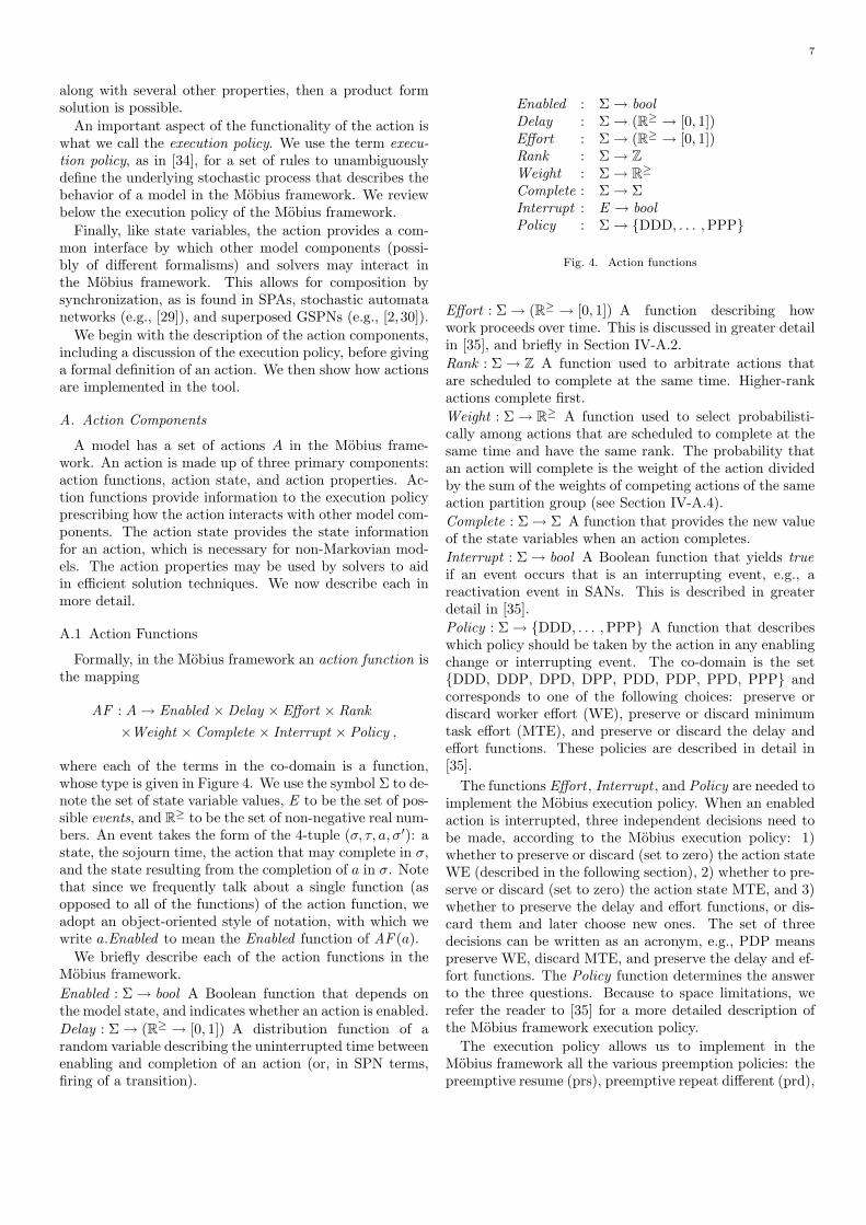
We briefly describe each of the action functions in theMobius framework.Enabled : Σ→ bool A Boolean function that depends onthe model state, and indicates whether an action is enabled.Delay : Σ→ (R≥ → [0, 1]) A distribution function of arandom variable describing the uninterrupted time betweenenabling and completion of an action (or, in SPN terms,firing of a transition).

Enabled : Σ→ boolDelay : Σ→ (R≥ → [0, 1])Effort : Σ→ (R≥ → [0, 1])Rank : Σ→ Z

Weight : Σ→ R≥

Complete : Σ→ ΣInterrupt : E → boolPolicy : Σ→ {DDD, . . . ,PPP}

Fig. 4. Action functions

Effort : Σ→ (R≥ → [0, 1]) A function describing howwork proceeds over time. This is discussed in greater detailin [35], and briefly in Section IV-A.2.Rank : Σ→ Z A function used to arbitrate actions thatare scheduled to complete at the same time. Higher-rankactions complete first.Weight : Σ→ R

≥ A function used to select probabilisti-cally among actions that are scheduled to complete at thesame time and have the same rank. The probability thatan action will complete is the weight of the action dividedby the sum of the weights of competing actions of the sameaction partition group (see Section IV-A.4).Complete : Σ→ Σ A function that provides the new valueof the state variables when an action completes.Interrupt : Σ→ bool A Boolean function that yields trueif an event occurs that is an interrupting event, e.g., areactivation event in SANs. This is described in greaterdetail in [35].Policy : Σ→ {DDD, . . . ,PPP} A function that describeswhich policy should be taken by the action in any enablingchange or interrupting event. The co-domain is the set{DDD, DDP, DPD, DPP, PDD, PDP, PPD, PPP} andcorresponds to one of the following choices: preserve ordiscard worker effort (WE), preserve or discard minimumtask effort (MTE), and preserve or discard the delay andeffort functions. These policies are described in detail in[35].

The functions Effort , Interrupt , and Policy are needed toimplement the Mobius execution policy. When an enabledaction is interrupted, three independent decisions need tobe made, according to the Mobius execution policy: 1)whether to preserve or discard (set to zero) the action stateWE (described in the following section), 2) whether to pre-serve or discard (set to zero) the action state MTE, and 3)whether to preserve the delay and effort functions, or dis-card them and later choose new ones. The set of threedecisions can be written as an acronym, e.g., PDP meanspreserve WE, discard MTE, and preserve the delay and ef-fort functions. The Policy function determines the answerto the three questions. Because to space limitations, werefer the reader to [35] for a more detailed description ofthe Mobius framework execution policy.

The execution policy allows us to implement in theMobius framework all the various preemption policies: thepreemptive resume (prs), preemptive repeat different (prd),

8

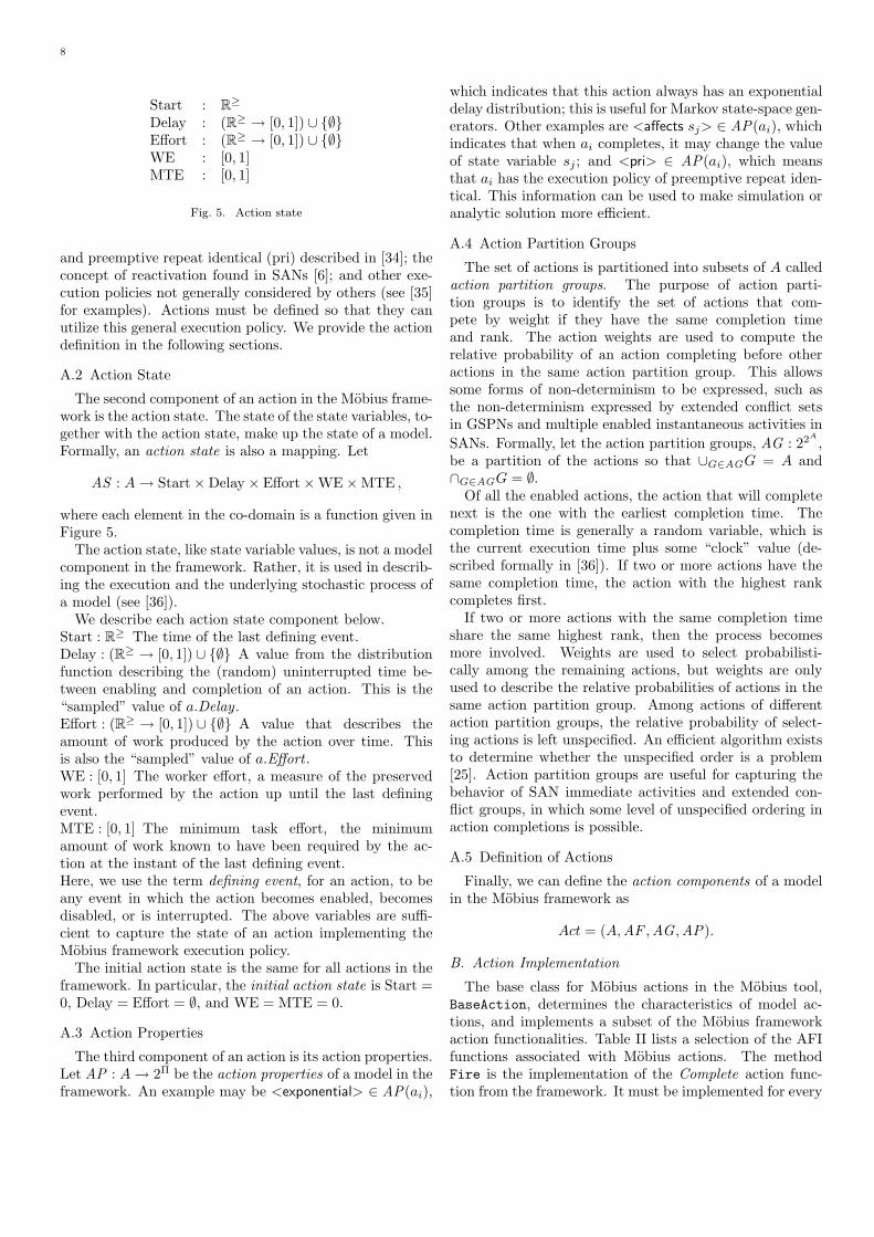
Start : R≥

Delay : (R≥ → [0, 1]) ∪ {∅}Effort : (R≥ → [0, 1]) ∪ {∅}WE : [0, 1]MTE : [0, 1]

Fig. 5. Action state

and preemptive repeat identical (pri) described in [34]; theconcept of reactivation found in SANs [6]; and other exe-cution policies not generally considered by others (see [35]for examples). Actions must be defined so that they canutilize this general execution policy. We provide the actiondefinition in the following sections.

A.2 Action State

The second component of an action in the Mobius frame-work is the action state. The state of the state variables, to-gether with the action state, make up the state of a model.Formally, an action state is also a mapping. Let

AS : A→ Start×Delay × Effort×WE×MTE ,

where each element in the co-domain is a function given inFigure 5.

The action state, like state variable values, is not a modelcomponent in the framework. Rather, it is used in describ-ing the execution and the underlying stochastic process ofa model (see [36]).

We describe each action state component below.Start : R≥ The time of the last defining event.Delay : (R≥ → [0, 1]) ∪ {∅} A value from the distributionfunction describing the (random) uninterrupted time be-tween enabling and completion of an action. This is the“sampled” value of a.Delay .Effort : (R≥ → [0, 1]) ∪ {∅} A value that describes theamount of work produced by the action over time. Thisis also the “sampled” value of a.Effort .WE : [0, 1] The worker effort, a measure of the preservedwork performed by the action up until the last definingevent.MTE : [0, 1] The minimum task effort, the minimumamount of work known to have been required by the ac-tion at the instant of the last defining event.Here, we use the term defining event, for an action, to beany event in which the action becomes enabled, becomesdisabled, or is interrupted. The above variables are suffi-cient to capture the state of an action implementing theMobius framework execution policy.

The initial action state is the same for all actions in theframework. In particular, the initial action state is Start =0, Delay = Effort = ∅, and WE = MTE = 0.

A.3 Action Properties

The third component of an action is its action properties.Let AP : A→ 2Π be the action properties of a model in theframework. An example may be <exponential> ∈ AP(ai),

which indicates that this action always has an exponentialdelay distribution; this is useful for Markov state-space gen-erators. Other examples are <affects sj> ∈ AP(ai), whichindicates that when ai completes, it may change the valueof state variable sj ; and <pri> ∈ AP(ai), which meansthat ai has the execution policy of preemptive repeat iden-tical. This information can be used to make simulation oranalytic solution more efficient.

A.4 Action Partition Groups

The set of actions is partitioned into subsets of A calledaction partition groups. The purpose of action parti-tion groups is to identify the set of actions that com-pete by weight if they have the same completion timeand rank. The action weights are used to compute therelative probability of an action completing before otheractions in the same action partition group. This allowssome forms of non-determinism to be expressed, such asthe non-determinism expressed by extended conflict setsin GSPNs and multiple enabled instantaneous activities inSANs. Formally, let the action partition groups, AG : 22A ,be a partition of the actions so that ∪G∈AGG = A and∩G∈AGG = ∅.

Of all the enabled actions, the action that will completenext is the one with the earliest completion time. Thecompletion time is generally a random variable, which isthe current execution time plus some “clock” value (de-scribed formally in [36]). If two or more actions have thesame completion time, the action with the highest rankcompletes first.

If two or more actions with the same completion timeshare the same highest rank, then the process becomesmore involved. Weights are used to select probabilisti-cally among the remaining actions, but weights are onlyused to describe the relative probabilities of actions in thesame action partition group. Among actions of differentaction partition groups, the relative probability of select-ing actions is left unspecified. An efficient algorithm existsto determine whether the unspecified order is a problem[25]. Action partition groups are useful for capturing thebehavior of SAN immediate activities and extended con-flict groups, in which some level of unspecified ordering inaction completions is possible.

A.5 Definition of Actions

Finally, we can define the action components of a modelin the Mobius framework as

Act = (A,AF ,AG ,AP).

B. Action Implementation

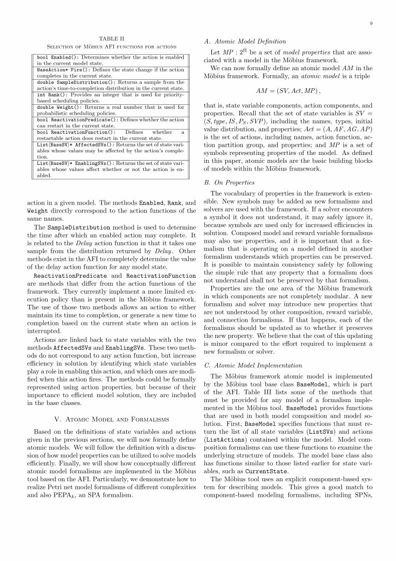
The base class for Mobius actions in the Mobius tool,BaseAction, determines the characteristics of model ac-tions, and implements a subset of the Mobius frameworkaction functionalities. Table II lists a selection of the AFIfunctions associated with Mobius actions. The methodFire is the implementation of the Complete action func-tion from the framework. It must be implemented for every

9

TABLE II

Selection of Mobius AFI functions for actions

bool Enabled(): Determines whether the action is enabledin the current model state.BaseAction* Fire(): Defines the state change if the actioncompletes in the current state.double SampleDistribution(): Returns a sample from theaction’s time-to-completion distribution in the current state.int Rank(): Provides an integer that is used for priority-based scheduling policies.double Weight(): Returns a real number that is used forprobabilistic scheduling policies.bool ReactivationPredicate(): Defines whether the actioncan restart in the current state.bool ReactivationFunction(): Defines whether arestartable action does restart in the current state.List〈BaseSV〉* AffectedSVs(): Returns the set of state vari-ables whose values may be affected by the action’s comple-tion.List〈BaseSV〉* EnablingSVs(): Returns the set of state vari-ables whose values affect whether or not the action is en-abled.

action in a given model. The methods Enabled, Rank, andWeight directly correspond to the action functions of thesame names.

The SampleDistribution method is used to determinethe time after which an enabled action may complete. Itis related to the Delay action function in that it takes onesample from the distribution returned by Delay . Othermethods exist in the AFI to completely determine the valueof the delay action function for any model state.ReactivationPredicate and ReactivationFunction

are methods that differ from the action functions of theframework. They currently implement a more limited ex-ecution policy than is present in the Mobius framework.The use of those two methods allows an action to eithermaintain its time to completion, or generate a new time tocompletion based on the current state when an action isinterrupted.

Actions are linked back to state variables with the twomethods AffectedSVs and EnablingSVs. These two meth-ods do not correspond to any action function, but increaseefficiency in solution by identifying which state variablesplay a role in enabling this action, and which ones are modi-fied when this action fires. The methods could be formallyrepresented using action properties, but because of theirimportance to efficient model solution, they are includedin the base classes.

V. Atomic Model and Formalisms

Based on the definitions of state variables and actionsgiven in the previous sections, we will now formally defineatomic models. We will follow the definition with a discus-sion of how model properties can be utilized to solve modelsefficiently. Finally, we will show how conceptually differentatomic model formalisms are implemented in the Mobiustool based on the AFI. Particularly, we demonstrate how torealize Petri net model formalisms of different complexitiesand also PEPAk, an SPA formalism.

A. Atomic Model Definition

Let MP : 2Π be a set of model properties that are asso-ciated with a model in the Mobius framework.

We can now formally define an atomic model AM in theMobius framework. Formally, an atomic model is a triple

AM = (SV,Act,MP) ,

that is, state variable components, action components, andproperties. Recall that the set of state variables is SV =(S, type, IS , PS ,SVP), including the names, types, initialvalue distribution, and properties; Act = (A,AF ,AG ,AP)is the set of actions, including names, action function, ac-tion partition group, and properties; and MP is a set ofsymbols representing properties of the model. As definedin this paper, atomic models are the basic building blocksof models within the Mobius framework.

B. On Properties

The vocabulary of properties in the framework is exten-sible. New symbols may be added as new formalisms andsolvers are used with the framework. If a solver encountersa symbol it does not understand, it may safely ignore it,because symbols are used only for increased efficiencies insolution. Composed model and reward variable formalismsmay also use properties, and it is important that a for-malism that is operating on a model defined in anotherformalism understands which properties can be preserved.It is possible to maintain consistency safely by followingthe simple rule that any property that a formalism doesnot understand shall not be preserved by that formalism.

Properties are the one area of the Mobius frameworkin which components are not completely modular. A newformalism and solver may introduce new properties thatare not understood by other composition, reward variable,and connection formalisms. If that happens, each of theformalisms should be updated as to whether it preservesthe new property. We believe that the cost of this updatingis minor compared to the effort required to implement anew formalism or solver.

C. Atomic Model Implementation

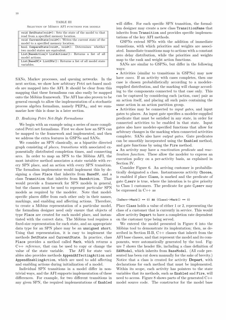
The Mobius framework atomic model is implementedby the Mobius tool base class BaseModel, which is partof the AFI. Table III lists some of the methods thatmust be provided for any model of a formalism imple-mented in the Mobius tool. BaseModel provides functionsthat are used in both model composition and model so-lution. First, BaseModel specifies functions that must re-turn the list of all state variables (ListSVs) and actions(ListActions) contained within the model. Model com-position formalisms can use these functions to examine theunderlying structure of models. The model base class alsohas functions similar to those listed earlier for state vari-ables, such as CurrentState.

The Mobius tool uses an explicit component-based sys-tem for describing models. This gives a good match tocomponent-based modeling formalisms, including SPNs,

10

TABLE III

Selection of Mobius AFI functions for models

void SetState(void*): Sets the state of the model to thatread from a specified memory location.void CurrentState(void*): Writes the current state of themodel to a specified memory location.bool CompareState(void*, void*): Determines whethertwo model states are equivalent.List〈BaseAction〉* ListActions(): Returns a list of allmodel actions.List〈BaseSV〉* ListSVs(): Returns a list of all model statevariables.

SANs, Markov processes, and queuing networks. In thenext section, we show how arbitrary Petri net-based mod-els are mapped into the AFI. It should be clear from thismapping that these formalisms can also easily be mappedonto the Mobius framework. The AFI has also proven to begeneral enough to allow the implementation of a stochasticprocess algebra formalism, namely PEPAk, and we sum-marize how this is done in a later section.

D. Realizing Petri Net-Style Formalisms

We begin with an example using a series of more compli-cated Petri net formalisms. First we show how an SPN canbe mapped to the framework and implemented, and thenwe address the extra features in GSPNs and SANs.

We consider an SPN classically, as a bipartite directedgraph consisting of places, transitions with associated ex-ponentially distributed completion times, and connectingarcs. In order to map an SPN to the Mobius AFI, themost intuitive method associates a state variable with ev-ery SPN place, and an action with every SPN transition.The formalism implementor would implement this by de-signing a class Place that inherits from BaseSV, and aclass Transition that inherits from BaseAction. Thatwould provide a framework for SPN models in general,but the classes must be used to represent particular SPNmodels as required by the modeler. Note that model-specific places differ from each other only in their names,markings, and enabling and affecting actions. Therefore,to create a Mobius representation of a particular model,the formalism designer need only ensure that objects oftype Place are created for each model place, and instan-tiated with the correct data. The Mobius tool requires afixed-size representation for each state, and an appropriatedata type for an SPN place may be an unsigned short.Using that representation, it is easy to implement themethods SetState and CurrentState. In practice, classPlace provides a method called Mark, which returns aC++ reference, that can be used to copy or change thevalue of the state variable. The AFI for state vari-ables also provides methods AppendAffectingAction andAppendEnablingAction, which are used to add affectingand enabling actions during initialization of a model.

Individual SPN transitions in a model differ in non-trivial ways, and the AFI supports implementation of thesedifferences. For example, for two different transitions inany given SPN, the required implementations of Enabled

will differ. For each specific SPN transition, the formal-ism designer may create a new class TransitionName thatinherits from Transition and provides specific implemen-tations of the key AFI methods.

GSPNs extend SPNs with the addition of immediatetransitions, with which priorities and weights are associ-ated. Immediate transitions map to actions with a constantzero delay distribution, while the priorities and weightsmap to the rank and weight action functions.

SANs are similar to GSPNs, but differ in the followingways:• Activities (similar to transitions in GSPNs) may nowhave cases. If an activity with cases completes, then onecase is chosen probabilistically according to a modeler-supplied distribution, and the marking will change accord-ing to the components connected to that case only. Thiscan be captured by considering each (action, case) pair asan action itself, and placing all such pairs containing thesame action in an action partition group.• Activities may be connected to input gates, and inputgates to places. An input gate specifies a modeler-suppliedpredicate that must be satisfied in any state, in order forconnected activities to be enabled in that state. Inputgates also have modeler-specified functions that allow forarbitrary changes in the marking when connected activitiescomplete. SANs also have output gates. Gate predicatescan be smoothly incorporated using the Enabled method,and gate functions by using the Fire method.• An activity may have a reactivation predicate and reac-tivation function. These allow the modeler to express anexecution policy on a per-activity basis, as explained inSection IV.

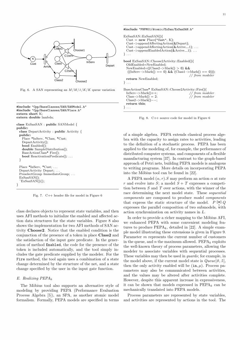
Consider Figure 6. An arriving customer is probabilis-tically designated a class. Instantaneous activity Chooseiis enabled if place Classi is marked and the predicate ofgate Ciserv is true, where the intention is to give priorityto Class 1 customers. The predicate for gate C2serv maybe expressed in C++ as

(InServ->Mark() == 0) && (Class1->Mark() == 0)

Place Class holds a value of either 1 or 2, representing theclass of a customer that is currently in service. This wouldallow activity Depart to have a completion rate dependenton the customer type being served.

We entered the model presented in Figure 6 into theMobius tool to demonstrate its implentation; then, as de-scribed in Section II-B, C++ classes that inherit from theAFI base classes, and that represent the model and its com-ponents, were automatically generated by the tool. Fig-ure 7 shows the header file, including a class definition ofSANModel, which inherits from BaseModel. (All code pre-sented has been cut down manually for the sake of brevity.)Notice that a class is created for activity Depart, withdeclarations for each method that must be implemented.Within its scope, each activity has pointers to the statevariables that its methods, such as Enabled and Fire, willneed to access. Figure 8 shows parts of the generated C++model source code. The constructor for the model base

11

Cust

K

Class1

Class2

DepartInServ

Choose1

Choose2

C1serv

C2serv

ArriveClass

Fig. 6. A SAN representing an M/M/1/K/K queue variation

#include "Cpp/BaseClasses/SAN/SANModel.h"#include "Cpp/BaseClasses/SAN/Place.h"extern short K;extern double lambda;

class ExSanSAN : public SANModel {public:

class DepartActivity : public Activity {public:

Place *InServ, *Class, *Cust;DepartActivity();bool Enabled();double SampleDistribution();BaseActionClass* Fire();bool ReactivationPredicate(); . . .}

Place *InServ, *Cust; . . .DepartActivity Depart; . . .PreselectGroup ImmediateGroup; . . .ExSanSAN();˜ExSanSAN(){};}

Fig. 7. C++ header file for model in Figure 6

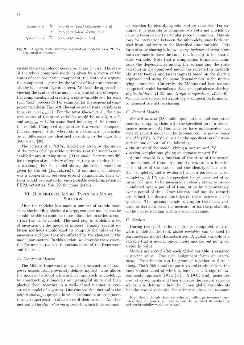
class declares objects to represent state variables, and thenuses AFI methods to initialize the enabled and affected ac-tion data structures for the state variables. Figure 8 alsoshows the implementation for two AFI methods of SAN ac-tivity Choose2. Notice that the enabled condition is theconjunction of the presence of a token in place Class2 andthe satisfaction of the input gate predicate. In the gener-ation of method Enabled, the code for the presence of thetoken is included automatically, and the tool simply in-cludes the gate predicate supplied by the modeler. For theFire method, the tool again uses a combination of a statechange determined by the structure of the net, and a statechange specified by the user in the input gate function.

E. Realizing PEPAk

The Mobius tool also supports an alternative style ofmodeling by providing PEPA (Performance EvaluationProcess Algebra [5]), an SPA, as another atomic modelformalism. Formally, PEPA models are specified in terms

#include "PNPM01/Atomic/ExSan/ExSanSAN.h"

ExSanSAN::ExSanSAN(){Cust = new Place("Cust", K);Cust−>appendAffectingAction(&Depart);Cust−>appendAffectingAction(&Arrive 1); . . .Cust−>appendEnabledAction(&Arrive 1); . . .} . . .

bool ExSanSAN::Choose2Activity::Enabled(){OldEnabled=NewEnabled;NewEnabled=((Class2−>Mark() > 0) &&((InServ−>Mark() == 0) && (Class1−>Mark() == 0)));

// from modelerreturn NewEnabled;} . . .

BaseActionClass* ExSanSAN::Choose2Activity::Fire(){InServ−>Mark()++; // from modelerClass−>Mark() = 2; // from modelerClass2−>Mark()−−;return this;} . . .

Fig. 8. C++ source code for model in Figure 6

of a simple algebra. PEPA extends classical process alge-bra with the capacity to assign rates to activities, leadingto the definition of a stochastic process. PEPA has beenapplied to the modeling of, for example, the performance ofdistributed computer systems, and components of a flexiblemanufacturing system [37]. In contrast to the graph-basedapproach of Petri nets, building PEPA models is analogousto writing programs. More details on incorporating PEPAinto the Mobius tool can be found in [22].

A PEPA model (α, r).S may perform an action α at rater and evolve into S ; a model S + T expresses a competi-tion between S and T over actions, with the winner of therace determining the next model state. These sequentialcomponents are composed to produce model componentsthat express the static structure of the model. P ��

LQ

expresses the parallel composition of two submodels, withaction synchronization on activity names in L.

In order to provide a richer mapping to the Mobius AFI,we enhanced PEPA with some convenient modeling fea-tures to produce PEPAk, detailed in [22]. A simple exam-ple model illustrating these extensions is given in Figure 9.Parameter m represents the current number of customersin the queue, and n the maximum allowed. PEPAk exploitsthe well-known theory of process parameters, allowing themodeler to associate variables with sequential processes.These variables may then be used in guards; for example, inthe model above, if the current model state is Queue[0 , 5 ],then the only activity enabled will be (in, µ). Process pa-rameters may also be communicated between activities,and the values may be altered after activities complete.However, despite this apparent increase in expressiveness,it can be shown that models expressed in PEPAk can bemechanically translated into PEPA models.

Process parameters are represented by state variables,and activities are represented by actions in the tool. The

12

Queue[m,n]def= [m > 0]⇒ (out, λ).Queue[m − 1 ,n]

+ [m < n]⇒ (in, µ).Queue′[m,n]

Queue′[m,n]def= (ref, ρ).Queue[m + 1 ,n]

Fig. 9. A queue with customer registration modeled as a PEPAksequential component

visible state variables of Queue[m,n] are {m,n}. The stateof the whole composed model is given by a vector of thestates of each sequential component; the state of a sequen-tial component is given by the values of its parameters andalso by its current algebraic term. We take the approach ofviewing the syntax of the model as a (static) tree of sequen-tial components, and creating a state variable svS for eachsuch “leaf” process S . For example, for the sequential com-ponent model in Figure 9, the entire set of state variables isthus {m,n, svQueue}. For the term Queue ′[3 , 5 ], the cur-rent values of the state variables would be m = 3, n = 5,and svQueue = 1 , for some fixed indexing of the terms ofthe model. Composed model state is a vector of sequen-tial component state, where state vectors with particularorder differences are identified according to the algorithmdetailed in [38].

The actions of a PEPAk model are given by the unionof the types of all possible activities that the model couldenable for any starting state. (If the model features two dif-ferent copies of an activity of type a, they are distinguishedas actions.) For the model above, the actions would begiven by the set {in, out, ref}. If our model of interestwas a cooperation between several components, then ac-tions would be created for each possible synchronization ofPEPA activities. See [22] for more details.

VI. Higher-level Model Types and Model

Solution

After the modeler has made a number of atomic mod-els as the building blocks of a large, complex model, she/heshould be able to combine these submodels in order to con-struct the whole model. The next step is to define a setof measures on the model of interest. Finally, several so-lution methods should exist to compute the value of themeasures and how they are affected by the changes in themodel parameters. In this section, we describe these essen-tial features as realized in various parts of the frameworkand the tool.

A. Composed Models

The Mobius framework allows the construction of com-posed models from previously defined models. This allowsthe modeler to adopt a hierarchical approach to modeling,by constructing submodels as meaningful units and thenplacing them together in a well-defined manner to con-struct a model of a system. One composition method is theaction-sharing approach, in which submodels are composedthrough superposition of a subset of their actions. Anothermethod is the state-sharing approach, which links submod-

els together by identifying sets of state variables. For ex-ample, it is possible to compose two Petri net models bycausing them to hold particular place in common. This al-lows for interaction between the submodels, since both canread from and write to the identified state variable. Thisform of state sharing is known as equivalence sharing, sinceboth submodels have the same relationship to the sharedstate variable. Note that a composition formalism main-tains the dependencies among the actions and the statevariables in the composed model (as reflected in methodslike AffectedSVs and EnablingSVs) based on the sharingapproach and using the same dependencies in the under-lying submodels. Currently, the Mobius tool features twocomposed model formalisms that use equivalence sharing:Replicate/Join [21, 39] and Graph composition [27, 39, 40].We have also developed a prototype composition formalismto demonstrate action sharing.

B. Reward Models

Reward models [28] build upon atomic and composedmodels, equipping them with the specification of a perfor-mance measure. At this time we have implemented onetype of reward model in the Mobius tool: a performancevariable (PV). A PV1 allows for the specification of a mea-sure on one or both of the following:• the states of the model, giving a rate reward PV• action completions, giving an impulse reward PV

A rate reward is a function of the state of the systemat an instant of time. An impulse reward is a functionof the state of the system and the identity of an actionthat completes, and is evaluated when a particular actioncompletes. A PV can be specified to be measured at aninstant of time, to be measured in steady state, to be ac-cumulated over a period of time, or to be time-averagedover a period of time. Once the rate and impulse rewardsare defined, the desired statistics on the measure must bespecified. The options include solving for the mean, vari-ance, or distribution of the measure, or for the probabilityof the measure falling within a specified range.

C. Studies

During the specification of atomic, composed, and re-ward models in the tool, global variables can be used toparameterize model characteristics. A global variable is avariable that is used in one or more models, but not givena specific value.

Models are solved after each global variable is assigneda specific value. One such assignment forms an experi-ment. Experiments can be grouped together to form astudy. The Mobius tool supports several study editors, themost sophisticated of which is based on a Design of Ex-periments approach (DOE [41]). A DOE study generatesa set of experiments and then analyzes the reward variablesolutions to determine how the chosen global variables af-fect the reward variables. Sensitivity analysis can measure

1Note that although these variables are called performance vari-ables, they are generic and can be used to represent dependabilityand performability variables as well.

13

the effects of all model parameters and their interactionson each solved reward variable. In addition, the model pa-rameter values that produce optimal reward variable valuescan be determined.

D. Solution Techniques

The Mobius tool currently supports two classes of solu-tion techniques: discrete event simulation and state-based,analytical/numerical techniques. Any model specified us-ing Mobius may be solved using simulation. Models thathave delays that are exponentially distributed, or have nomore than one concurrently enabled deterministic delay,may be solved using a variety of analytic techniques appliedto a generated state space. The simulator and state-spacegenerator operate on models only through the Mobius AFI.Formalism-specific analysis and property discovery is per-formed by the formalism editor. Mobius allows formalism-specific solution techniques in the form of property-specificsolvers. For example, analytic solution using state-spacegeneration requires the properties described above. In or-der to evaluate the overhead resulting from the generalityof the Mobius framework, we have compared the perfor-mance of the simulators in UltraSAN and Mobius [42]. Weobserved that the amount of overhead is negligible com-pared to runtime differences caused by other factors, suchas the algorithm used by the solver and the optimizationtechniques used in the implementation.

D.1 State-Space Generator

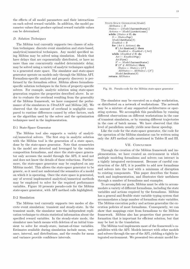
The Mobius tool also supports a variety of analyti-cal/numerical solvers. The first step in analytic solutionwith the Mobius tool is the generation of a state space,done by the state-space generator. Note that symmetriesin the model are detected and leveraged by the variouscomposition formalisms, and since the state-space genera-tor only accesses the model through the AFI, it need notand does not know the details of these reductions. Further-more, the state-space generator may be employed on anyMobius model. This allows the state-space generator to begeneric, so it need not understand the semantics of a modelon which it is operating. Once the state space is generated,any of several implemented analytical/numerical methodsmay be employed to solve for the required performancevariables. Figure 10 presents pseudo-code for the Mobiusstate-space generator, with AFI method calls highlighted.

D.2 Simulation

The Mobius tool currently supports two modes of dis-crete event simulation: transient and steady-state. In thetransient mode, the simulator uses the independent repli-cation technique to obtain statistical information about thespecified reward variables. In the steady-state mode, thesimulator uses batch means with deletion of an initial tran-sient to solve for steady-state, instant-of-time variables.Estimates available during simulation include mean, vari-ance, interval, and distributions, and the results for meanand variance provide confidence intervals.

State-Space Generator(Model)AllStates← ∅States← {Model.CurrentState()}Actions←Model.ListActions()while (States 6= ∅) doS ← States.Pop()Model.SetState(S)Enabled← ∅for (Act ∈ Actions) do

if (Act.Enabled()) thenEnabled← Enabled ∪ {Act}

while (Enabled 6= ∅) doAct← Enabled.Pop()Act.Fire()S′ ←Model.CurrentState()if (S′ 6∈ AllStates) thenStates← States ∪ {S′}AllStates← AllStates ∪ {S′}

Model.SetState(S)return AllStates

Fig. 10. Pseudo-code for the Mobius state-space generator

The simulator may be executed on a single workstation,or distributed on a network of workstations. The networkmay be a mixture of any supported architectures or oper-ating systems. We accomplish this parallelism by runningdifferent observations on different workstations in the caseof transient simulation, or by running different trajectoriesin the case of batch means. We have observed that thislevel of parallelism usually yields near-linear speedup.

Like the code for the state-space generator, the code forthe operation of the Mobius simulator can be written usingonly the AFI method calls mentioned in Tables II and III.

VII. Conclusion

Through the creation of the Mobius framework and im-plementation, we have created an environment in whichmultiple modeling formalisms and solvers can interact ina tightly integrated environment. Because of careful con-struction of the AFI, it is possible to add new formalismsand solvers into the tool with a minimum of disruptionto existing components. This paper describes the frame-work and implementation, and illustrates their usefulnessthrough a number of formalisms and examples.

To accomplish our goals, Mobius must be able to accom-modate a variety of different formalisms, including the statevariables and actions required by the formalisms. Mobiushas a general and flexible state variable typing system thataccommodates a large number of formalism state variables.The Mobius execution policy and actions generalize the ex-ecution policies of most formalisms. Consequently, we canshow that mappings exist from formalisms to the Mobiusframework. Mobius also has properties that preserve in-formation that is important for efficient solution, but thatmay be lost in the translation.

The Mobius tool implements most of the framework’s ca-pabilities with the AFI. Models interact with other modelsand solvers through the use of the AFI, yielding a tightly in-tegrated environment. We presented two atomic model for-

14

malisms that have been implemented in the tool: SANs andPEPAk. We also showed how other parts of the tool, suchas reward models, composed models, studies, and solvers,interact with atomic models without regard to the formal-ism that was used to create them.

New formalisms and solvers are currently under devel-opment by ourselves and by others. Others can benefit byleveraging existing formalisms and tools. For example, aformalism developer does not need to recreate a distributedsimulation solver or a state-space generator, or compositionformalisms, for the formalism to be useful. Our recent suc-cesses bode well for Mobius’s use as a vehicle for others toimplement new modeling formalisms and solution methods,and we welcome participation by others in this endeavor.

ACKNOWLEDGMENTS

We would like to acknowledge the contributions of theformer members of the Mobius group: Amy L. Christensen,G. P. Kavanaugh, John M. Sowder, Aaron J. Stillman, andAlex L. Williamson. We would also like to thank JennyApplequist for her editorial assistance.

References

[1] F. Baskett, K. M. Chandy, R. R. Muntz, and F. G. Palacios,“Open, closed, and mixed networks of queues with differentclasses of customers,” Journal of the Association for ComputingMachinery, vol. 22, no. 2, pp. 248–260, Apr. 1975.

[2] S. Donatelli, “Superposed generalized stochastic Petri nets: Def-inition and efficient solution,” in Application and Theory ofPetri Nets 1994, LNCS 815 (Proc. 15th International Confer-ence on Application and Theory of Petri Nets, Zaragoza, Spain),R. Valette, Ed., pp. 258–277. Springer-Verlag, June 1994.

[3] G. Chiola, G. Bruno, and T. Demaria, “Introducing a color for-malism into generalized stochastic Petri nets,” in Proc. 9th Eu-ropean Workshop on the Application and Theory of Petri Nets,Venice, Italy, June 1988, pp. 202–215.

[4] M. K. Molloy, “Performance analysis using stochastic Petrinets,” IEEE Trans. on Comp., vol. 31, pp. 913–917, Sept. 1982.

[5] J. Hillston, A Compositional Approach to Performance Mod-elling, Cambridge University Press, Cambridge, 1996.

[6] J. F. Meyer, A. Movaghar, and W. H. Sanders, “Stochastic ac-tivity networks: Structure, behavior, and application,” in Proc.International Workshop on Timed Petri Nets, Torino, Italy, July1985, pp. 106–115.

[7] W. H. Sanders, “Integrated frameworks for multi-level andmulti-formalism modeling,” in Proceedings of the 8th Inter-national Workshop on Petri Nets and Performance Models,Zaragoza, Spain, Sept. 1999, pp. 2–9.

[8] B. R. Haverkort, “Performability evaluation of fault-tolerantcomputer systems using DyQN-Tool+,” International Journalof Reliability, Quality, and Safety Engineering, vol. 2, no. 4, pp.383–404, 1995.

[9] G. Chiola, G. Franceschinis, R. Gaeta, and M. Ribaudo, “Great-SPN 1.7: Graphical Editor and Analyzer for Timed and Stochas-tic Petri Nets,” Performance Evaluation, vol. 24, no. 1–2, pp.47–68, Nov. 1995.

[10] M. Ajmone Marsan, G. Balbo, and G. Conte, “A class of gen-eralized stochastic Petri nets for the performance evaluation ofmultiprocessor systems,” ACM Transactions on Computer Sys-tems, vol. 2, pp. 93–122, 1984.

[11] W. H. Sanders, W. D. Obal II, M. A. Qureshi, and F. K. Wid-janarko, “The UltraSAN modeling environment,” PerformanceEvaluation, vol. 24, no. 1, pp. 89–115, Oct. 1995.

[12] G. Ciardo and K. S. Trivedi, “SPNP: The stochastic Petri netpackage (version 3.1),” in Proceedings of the 1st InternationalWorkshop on Modeling, Analysis and Simulation of Computerand Telecommunication Systems (MASCOTS’93), San Diego,California, Jan. 1993, pp. 390–391.

[13] G. Ciardo, A. Blakemore, P. F. J. Chimento, J. K. Muppala, andK. S. Trivedi, “Automated generation and analysis of Markov

reward models using stochastic reward nets,” in Linear Algebra,Markov Chains, and Queueing Models, C. Meyer and R. J. Plem-mons, Eds., pp. 141–191. Heidelberg: Springer-Verlag, 1993.

[14] R. M. L. R. Carmo, L. R. de Carvalho, E. de Souza e Silva,M. C. Diniz, and R. R. Muntz, “TANGRAM-II,” in ComputerPerformance Evaluation: Modelling Techniques and Tools: Pro-ceedings of the 9th International Conference, Raymond Marie,Brigitte Plateau, Maria Calzarossa, and Gerardo Rubino, Eds.,St. Malo, France, June 1997, pp. 6–18.

[15] R. J. Pooley, “The integrated modelling support environment:A new generation of performance modelling tools,” in ComputerPerformance Evaluation: Modelling Techniques and Tools: Pro-ceedings of the 5th International Conference, G. Balbo andG. Serazzi, Eds., Torino, Italy, Feb. 1991, pp. 1–15.

[16] R. Fricks, C. Hirel, S. Wells, and K. Trivedi, “The developmentof an integrated modeling environment,” in Proceedings of theWorld Congress on Systems Simulation (WCSS ’97), Singapore,Sept. 1997, pp. 471–476.

[17] Aad P. A. van Moorsel and Yiqing Huang, “Reusable soft-ware components for performability tools, and their utilizationfor web-based configuration tools,” in Computer PerformanceEvaluation: Modelling Techniques and Tools: Proceedings of the10th International Conference, R. Puigjaner, N. N. Savino, andB. Serra, Eds., Palma de Mallorca, Spain, Sept. 1998, pp. 37–50.

[18] R. A. Sahner, K. S. Trivedi, and A. Puliafito, Performanceand Reliability Analysis of Computer Systems, An Example-Based Approach Using the SHARPE Software Package, Kluwer,Boston, 1996.

[19] G. Ciardo and A. S. Miner, “SMART: Simulation and Marko-vian analyzer for reliability and timing,” in Tool Descriptionsfrom the 9th Int. Conf. on Modelling Techniques and Tools forComputer Performance Evaluation (TOOLS ’97) and the 7thInternational Workshop on Petri Nets and Performance Mod-els (PNPM ’97), St. Malo, France, June 1997, pp. 41–43.

[20] F. Bause, P. Buchholz, and P. Kemper, “A toolbox for functionaland quantitative analysis of DEDS,” in Computer PerformanceEvaluation: Modelling Techniques and Tools: Proc. of the 10thInt. Conf., R. Puigjaner, N. N. Savino, and B. Serra, Eds., Palmade Mallorca, Spain, Sept. 1998, pp. 356–359.

[21] W. H. Sanders and J. F. Meyer, “Reduced base model construc-tion methods for stochastic activity networks,” IEEE Journal onSelected Areas in Communications, special issue on Computer-Aided Modeling, Analysis, and Design of Communication Net-works, vol. 9, no. 1, pp. 25–36, Jan. 1991.

[22] G. Clark and W. H. Sanders, “Implementing a stochastic pro-cess algebra within the Mobius modeling framework,” in Pro-cess Algebra and Probabilistic Methods: Performance Modellingand Verification: Proc. of the Joint International Workshop,PAPM-PROBMIV 2001, Aachen, Germany, September 2001,vol. 2165 of Lecture Notes In Computer Science, pp. 200–215,Berlin: Springer.

[23] D. D. Deavours and W. H. Sanders, “An efficient disk-based toolfor solving large Markov models,” Performance Evaluation, vol.33, pp. 67–84, 1998.

[24] D. D. Deavours and W. H. Sanders, “‘On-the-fly’ solution tech-niques for stochastic Petri nets and extensions,” IEEE Trans.on Soft. Eng., vol. 24, no. 10, pp. 889–902, Oct. 1998.

[25] D. D. Deavours and W. H. Sanders, “An efficient well-specifiedcheck,” in Proceedings of the 8th International Workshop onPetri Nets and Performance Models (PNPM ’99), Zaragoza,Spain, Sept. 1999, pp. 124–133.

[26] W. D. Obal II and W. H. Sanders, “State-space support for path-based reward variables,” in Proc. 3rd Ann. IEEE InternationalComputer Performance and Dependability Symposium (IPDS’98), Durham, North Carolina, Sept. 1998, pp. 228–237.

[27] W. D.. Obal II and W. H. Sanders, “Measure-adaptive state-space construction methods,” Performance Evaluation, vol. 44,pp. 237–258, Apr. 2001.

[28] W. H. Sanders and J. F. Meyer, “A unified approach for specify-ing measures of performance, dependability, and performability,”in Dependable Computing for Critical Applications, A. Avizie-nis, J. Kopetz, and J. Laprie, Eds., vol. 4 of Dependable Com-puting and Fault-Tolerant Systems, pp. 215–237. Heidelberg:Springer-Verlag, 1991.

[29] B. Plateau and K. Atif, “A methodology for solving Markovmodels of parallel systems,” IEEE Journal on Software Engi-neering, vol. 17, no. 10, pp. 1093–1108, 1991.

[30] P. Kemper, “Numerical analysis of superposed GSPNs,” in Sixth

15

International Workshop on Petri Nets and Performance Models(PNPM ’95), Durham, North Carolina, Oct. 1995, pp. 52–61.

[31] G. Ciardo and K. S. Trivedi, “A decomposition approach forstochastic reward net models,” Performance Evaluation, vol.18, pp. 37–59, 1993.

[32] J. M. Doyle, “Abstract model specification using the Mobiusmodeling tool,” M.S. thesis, University of Illinois at Urbana-Champaign, Jan. 2000.

[33] C. H. Sauer and Edward A. MacNair, Simulation of ComputerCommunication Systems, Prentice-Hall, Inc., Englewood Cliffs,New Jersey, 1983.

[34] A. Bobbio, A. Puliafito, and M. Telek, “A modeling frameworkto implement preemption policies in non-Markovian SPNs,”IEEE Transactions on Software Engineering, vol. 26, no. 1, pp.36–54, Jan. 2000.

[35] D. D. Deavours and W. H. Sanders, “The Mobius executionpolicy,” in Proceedings of Petri Nets and Performance Models(PNPM 2001), Aachen, Germany, Sept. 2001, pp. 135–144.

[36] Daniel D. Deavours, Formal Specification of the Mobius Model-ing Framework, Ph.D. thesis, University of Illinois at Urbana-Champaign, Oct. 2001.

[37] D. R. W. Holton, “A PEPA specification of an industrial produc-tion cell,” The Computer Journal, vol. 38, no. 7, pp. 542–551,1995.

[38] S. Gilmore, J. Hillston, and M. Ribaudo, “An efficient algorithmfor aggregating PEPA models,” IEEE Transactions on SoftwareEngineering, vol. 27, no. 5, pp. 449–464, 2001.

[39] G. Clark, T. Courtney, D. Daly, D. D. Deavours, S. Derisavi,J. M. Doyle, W. H. Sanders, and P. G. Webster, “The Mobiusmodeling tool,” in Proceedings of Petri Nets and PerformanceModels (PNPM 2001), Aachen, Germany, Sept. 2001, pp. 241–250.

[40] A. J. Stillman, “Model composition within the Mobius model-ing framework,” M.S. thesis, University of Illinois at Urbana-Champaign, 1999.

[41] D. Montgomery, Design and Analysis of Experiments, JohnWiley & Sons, Inc., 5th edition, 2001.

[42] A. Williamson, “Discrete event simulation in the Mobius mod-eling framework,” M.S. thesis, University of Illinois at Urbana-Champaign, 1998.

Daniel D. Deavours received his Bachelordegree in Computer Engineering in 1995, Mas-ters in Electrical Engineering in 1997, andPh.D. in Electrical Engineering in 2001, allfrom the University of Illinois. He is currentlya Research Assistant Professor at the Univer-sity of Kansas. His research interests includestochastic modeling tools and numerical solu-tion techniques to Markov chains.

Graham Clark is a software engineer at Cit-rix Systems Inc. in Columbia, MD. He re-ceived his Ph.D. and Bachelor degrees in Com-puter Science from the University of Edin-burgh, Scotland. While working in the PER-FORM group at the University of Illinois, Gra-ham developed the Mobius framework map-ping and tool support for the stochastic processalgebra, PEPA.

Tod Courtney received his Bachelor degree inComputer Engineering in 1994 and his Mastersin Electrical Engineering in 1996, both fromthe University of Illinois. He is a research pro-grammer at the University of Illinois. His inter-ests include stochastic modeling software andfault tolerant middleware.

David Daly received his Bachelor degree inComputer Engineering from Syracuse Univer-sity in 1998, and his Masters in Electrical Engi-neering from the University of Illinois in 2001.He is currently a Ph.D. student in ElectricalEngineering at the University of Illinois. Hisresearch interests include the stochastic per-formability analysis and the decomposition oflarge models.

Salem Derisavi received his Bachelor degreein Computer Engineering in 1999 from SharifUniversity of Technology, Iran. He is currentlya Ph.D. student in Computer Science at theUniversity of Illinois. His research interestsinclude designing and implementing efficientdata structures and algorithms for functionaland numerical analysis of models.

Jay M. Doyle received his Bachelor degreein Computer Engineering from Syracuse Uni-versity in 1997, and his Masters in ElectricalEngineering from the University of Illinois in2000. He currently works as a software engi-neer in Honeywell’s Industrial Automation andControl group in Fort Washington, PA.

William H. Sanders received his B.S.E. inComputer Engineering (1983), his M.S.E. inComputer, Information, and Control Engineer-ing (1985), and his Ph.D. in Computer Scienceand Engineering (1988) from the University ofMichigan. He is currently a Professor in theDepartment of Electrical and Computer Engi-neering and the Coordinated Science Labora-tory at the University of Illinois. He is Chairof the IEEE TC on Fault-Tolerant Computingand Vice-Chair of IFIP Working Group 10.4 on

Dependable Computing. In addition, he serves on the Board of Direc-tors of ACM Sigmetrics and the editorial board of IEEE Transactionson Reliability, and is the Area Editor for Simulation and Modeling ofComputer Systems for the ACM Transactions on Modeling and Com-puter Simulation. He is a Fellow of the IEEE and a member of theIEEE Computer, Communications, and Reliability Societies, as wellas the ACM, IFIP Working Group 10.4 on Dependable Computing,Sigma Xi, and Eta Kappa Nu.

Dr. Sanders’s research interests include performance/dependabilityevaluation, dependable computing, and reliable distributed systems.He has published more than 100 technical papers in those areas.

Patrick Webster received his Bachelor de-gree in Mathematics from Rockford College in1992, his Masters in Applied Mathematics fromthe University of Illinois in 1994, and is finaliz-ing his Masters in Electrical Engineering, alsofrom the University of Illinois. He is currently aDesign Engineer at ARM, Inc. in Austin TX.